Asymptotic analysis of a cohesive crack: 1. Theoretical background

International Journal of Fracture 55:153-177, 1992. © 1992 Kluwer Academic Publishers. Printed in the Netherlands. 153

Asymptotic analysis of a cohesive crack: 1. Theoretical background

J. PLANAS and M. ELICES Departamento de Ciencia de Materiales, Escuela de Ingenieros de Caminos. Universidad Polit~cnica de Madrid, 28040-Madrid, Spain

Received 30 October 1990; accepted 30 September 1991

Abstract. A method to analyze the evolution of a cohesive crack, particularly appropriate for asymptotic analysis, is presented. Detailed descriptions of the zeroth order and first order asymptotic approaches are given and from these results the far field equivalent elastic crack theorem is derived. An analytically soluble example, the Griflith crack, and a simple model, the Dugdale model, are used to exemplify the results.

1. Introduction

When a crack is created in a material such as concrete, soil or a ceramic, and the material is stressed, a situation develops whereby the crack extends and its faces become bridged by unbroken ligaments whose average behaviour can be represented by a decreasing stress versus increasing crack face opening relationship. In this sense, the material can be regarded as being s t ra in sof tening. This situation can be modelled by a cohes ive zone, coplanar with the crack, where the restraining - or cohes ive - forces reflect the strain-softening characteristics of the material under consideration. In this context the cohesive zone model, originally conceived by [1], has been used extensively in investigations that allow for non-linearity of material behaviour in the vicinity of a crack tip. A review of crack and band models for strain softening materials was recently published by the authors [3].

Since the pioneering work of Barenblatt [1], where the cohesive zone was considered very small compared with the size of the crack, a large amount of work has been done extending such concept to polymers, ceramics and composite materials, where the cohesive zone need no longer remain small. As a consequence, apparently different models have emerged with cohesive forces renamed frictional, bridging, or restraining forces. Although the physical origin of these forces is clearly different, most of such models can be analyzed in a simple and unified way using the proposed method and the meaning of a cohesive crack should be understood in this general sense.

The present paper addresses the problem of cohesive crack growth in a strain softening material with the objective of studying the asymptotic behaviour: i.e. cases in which the size of the structure is much larger than the cohesive zone. With this objective in mind, in the next section the general problem is formulated as a weighted superposition of solutions of auxiliary linear elastic fracture mechanics problems and is reduced to solving a functional integral equation. Section 3 deals with the asymptotic analysis. It is shown that when all the functions appearing in the integral equation are approximated by a functional polynomial of degree N in an asymptotically vanishing variable, the previous functional integral equation splits into N + 1 integral equations which allow calculation of the N + 1 coefficients of the truncated series. Sections 4 and 5 are devoted to analysing the zeroth and first order asymptotic approaches. In these sections, besides evaluation of the general solution, the main characteris-

154 J. Planas and M. Elices

tics of the near fields - inside and around the cohesive zone and of the far fields are discussed.

In addition to providing a basis to set computational procedures for particular geometries, the formulation appears to be powerful enough to prove theorems valid for any geometry. The essential one proves that, to first order approximation, a far field equivalent elastic crack exists giving the same far fields as the actual nonlinear problem and a general expression for the corresponding effective crack extension is obtained. From this theorem, other interesting results are found.

2. Formulation of the general cohesive crack problem

2.1. The cohesive crack model

Different versions of cohesive crack models have been applied successfully to interpret the cracking behaviour of solids; Barenblatt used this model in a small region near the crack tip, offering an alternative to the Griffith model for brittle solids (see, for example, Goodier [4]). Dugdale [2] proposed a mathematically similar but conceptually different model with constant cohesive stress. A new interpretation of this concept was made by Rice [9] who for elastic materials assumed the restraining stress as a function of the separation distance, relating both values to J. Since then, cohesive cracks have been used to model plasticity, crazes in polymers, softening in rocks and concrete, and reinforcement in composite materials.

The formulation of a cohesive crack problem usually rests - more or less explicitly - on the

following hypotheses:

H 1. Loading. Loading is restricted to monotonic mode I crack growth, achieved by considering symmetric loading on a symmetric specimen. Furthermore, the loading is assumed to be

proportional. H2. Bulk behaviour. The behaviour of the bulk material is assumed to be isotropic linear elastic -

with Young's modulus E and Poisson's ratio v - as long as the major principal stress does

not reach a critical value ~R, the tensile strength or critical stress. H3. Crack initiation. When the maximum principal stress reaches aR, fracture is initiated and

strain localization takes place in what is called the Fracture Process Zone (FPZ). The FPZ is modelled as a cohesive crack where the strain localization is idealized as a displacement jump or crack opening, while cohesive stresses simulate the softening behaviour.

H4. Crack evolution. Once the cohesive crack has formed, the stress transferred through the crack faces is assumed to depend upon the relative displacement of the crack faces. For monotonic crack opening, the stress normal to the crack plane a is supposed to be given by a single-valued, non-negative function of the crack opening w, i.e.

a = F ( w ) where F(0)=trR and F(w)>lO. (2.1)

The material function F(w) - usually called the softening curve - together with E and v, suffice to characterize the material behaviour, as far as monotonic mode I is concerned. In practice, the values of F(w) are assumed to be zero for crack openings exceeding a critical

crack opening we.

Asymptotic analysis of a cohesive crack 155

The work needed to open monotonically a unit surface of crack, the specific work supply, is also a material function given by

Wv(w) = F(w') dw'. (2.2)

The specific work supply needed to open fully a unit surface of crack is a material property called the specific fracture energy Gv (or, simply, fracture energy), i.e.

fo fo G~ = F(w') dw' = F(w') dw'. (2.3)

From the material parameters E, v, aR and GF, two independent parameters having dimensions of length are introduced: The first was called characteristic length by Hillerborg [5] and defined as

GvE' lch-- cr~ ' (2.4)

where E' is the generalized Young's modulus; E' = E/(1 - v z) for plane strain and E' = E for generalized plane stress. The second parameter called characteristic crack opening, is defined as

GF Wch = - - . (2.5)

O- R

Following the previous hypotheses, consider a symmetric and symmetrically loaded plane body partially sketched in Fig. 1, which had an initial crack of length A0 on its symmetry line - taken

L X2

• .,,.-- X 1

I_ Ao ~ ' - - T - -

I -¢ C L

Fig. 1. Notation used for the cohesive crack problem and the auxiliary non-cohesive crack.


to coincide with the X~ axis - ahead of which a cohesive strip of length R has developed. It is specifically assumed that the loading is applied on the external boundary so that the initial crack surfaces are stress free and body forces are negligible. The proportionality of loading may be stated by saying that the traction vector distribution on the external boundary is proportional to a given dimensionless vector-valued function B~(Xj) bearing the appropriate symmetry properties. The proportionality factor, having dimensions of stress, will be called the nominal

stress, aN. Since the bulk of the material remains linear elastic, we may formulate the problem

introducing a biharmonic Airy stress function A(Xi) so that the stresses are given by

t~2A ~32A a~j = 6i~ C~XkC3X k OX~OX~ (2.6)

and equilibrium and compatibility conditions are automatically satisfied. The biharmonicity condition may be achieved in the standard way by using the complex potential formalism, but this will not be needed here.

The boundary conditions to be satisfied by the solution may be stated as follows: On the external boundary, proportional loading as previously stated,

a~j(Xk)nj(Xk) = aNBi(XR) (2.7)

Along the initial crack line the normal stress must be zero (the tangential stress is automatically zero due to symmetry conditions), hence, according to the axes shown in Fig. 1,

o '22 (X1 , 0) = 0 for X1 < Xo. (2.8)

On the cohesive zone, (2.1) must be satisfied, hence:

o'22(X1, 0) = F[w(X1) ] for Xo < X~ ~< R + Xo (2.9)

where w(X1) is the crack opening distribution:

w(Xl) = u2(X~, 0 +) - u2(X,, 0 - ) . (2.10)

On the remaining undisturbed ligament, the crack opening must vanish

w(X1)=O for X I > R + X o . (2.11)

These boundary conditions are sufficient to give a unique solution for any load and any cohesive zone length. However, such a solution would in general display a stress singularity at the cohesive crack tip, which violates hypothesis H3 stating that the maximum principal stress allowed by the body is aR. We need, therefore, a further equation abolishing this singularity,

which may be written as

lira [w/~'az2(Xo + R + e, 0)] = 0 (e > 0). (2.12) e~0


The boundary conditions (2.7) to (2.11) and the boundedness condition (2.12) are enough to find the complete solution of the elastic fields and the external load for a given cohesive zone length.

2.2. Auxiliary functions and superposition method

The cohesive crack problem can be re-formulated using a weighted superposition of solutions for a uniparametric family of auxiliary linear elastic fracture mechanics problems, a technique that proved useful for the asymptotic analysis as will be seen in the next section. The selection of the auxiliary problem is based on the evidence that the elastic solution for a crack, coplanar with the cohesive crack, symmetrically loaded on the external boundary and having arbitrary length C, so that Ao ~< C ~< Ao + R, (see Fig. 1), satisfies conditions (2.8) and (2.11), and it may also be chosen to satisfy a condition proportional to (2.7).

We denote a s AA(X1, X2; C), O'22A(X1, 0; C) and wa(X~; C) the solutions of the Airy stress function, stresses normal to the crack plane and crack openings satisfying the following conditions, corresponding to the elastic crack of length C subjected to a nominal stress equal to aR:

On the external boundary

aija(Xk) nj(Xk) = anBi(Xk) (2.13)

Along the crack line (see Fig. 1),

O'22A(X1, 0; C) = 0 for X~ < C, (2.14)

WA(X1; C) = 0 for X1 i> C. (2.15)

Since, as shown by (2.14) and (2.15), the auxiliary solution satisfies (2.8) and (2.11) for any C in the interval Ao ~< C ~< Ao + R, so does any weighted sum of such solutions, and we may look for a solution having the general form

I A o + R

A(XI, X2) = Aa(Xt, X2; C)Q(C)dC + MAA(X,, X2; Ao + R), J Ao

(2.16)

where Q(C) dC is a dimensionless, by now arbitrary, weight distribution on (Ao, Ao + R) and M is a dimensionless constant. The problem is now reduced to establishing the governing equations for Q(C)dC and M, by imposing the remaining conditions (2.7), (2.9) and (2.12).

We first notice that the solution factorised by M, in (2.16), corresponds to the solution for an elastic crack of length Ao + R and displays a stress singularity at X1 = Xo + R, so that for the boundedness condition (2.12) to be verified it is necessary that

M = 0. (2.17)

For boundary condition (2.7) to hold, we must have, according to (2.13), (2.16) and (2.17)

I A o + R

aN = aR Q(C) dC, d Ao

(2.18)


where it is assumed that differential operators in (2.6) commute with the integral in (2.16). The only remaining boundary condition to impose is given by (2.9) which leads to an integral

equation determining the weight distribution Q(C)dC. To obtain this equation, notice that the normal stresses and crack openings are given by the following integral expressions:

IA ° + R 0"22(X1, 0 ) = o ' 2 2 A ( X 1 , 0; C)Q(C)dC, o

(2.19)

I Ao+R

w(X1) = WA(X1; C)Q(C) dC, (2.20) d Ao

where the auxiliary solutions 022 A and Wa are assumed to be known from elastic analyses. Imposing condition (2.9), the following integral equation is found:

to+, Fro+. ] O22A(X1, 0"~ C ) Q ( C ) d C = f wa(Xl; C)Q(C)dC , d Ao Ld Ao

(2.21)

where Ao < C < Ao + R and Xo < X1 ~< Xo + R. This integral equation is, in general, nonlinear and, moreover, the auxiliary solutions aZZA and WA are not available in closed form for most geometries. There are, however, some exceptions of great theoretical interest, such as the one considered in the next example.

2.3. An analytically soluble example

One of such exceptions is the Griffith crack, an infinite plate with a centre crack of length 2Ao subjected to uniform remote stress aN normal to the crack plate. Assuming symmetric cohesive zones at both crack ends, the auxiliary problem is that of a crack of length 2C without restraining stresses, for which the solutions for stresses and crack openings along the positive X1 axis (Fig. 2) are known to be:

0"22A(X1, O; C ) = °'R H(X1 - C), (2.22) ~/1 - (C/X1) 2

w A X , ; c ) = t-I(C - x l ) , (2.23)

where H(X) denotes the Heaviside step distribution. From this and (2.19) and (2.20), the complete solution for stresses and crack openings along

the positive Xx axis are,

~ao+R H(XI -- C)Q(C) dC a22(X1, 0) = JAo ~/1 (C/Xa) 2 O" R - - , (2.24)

4a R [Ao+R w(Xx) = ~7- JAo H(C -- X1) ~ £ -- X~ Q(C) dC (2.25)


ON

ITTTITTTT ~ X 2

i

i

Ii tll°; TIll 2 C -

× !

i i t t t t ( t l t O N

Fig. 2. Griffith crack with symmetric cohesive zones.

and the integral equation (2.21) is then transformed into

f A : I Q ( C ) dC I4aRfX I°+R ] = F -~, Q(C)w/~ - ~ dC aR o ~ /1 - ( C / X 1 ) 2 E ~

(2.26)

For a general softening function, this integral equation has no analytic solution. However, an analytic solution does exist for Dugdale - or rectangular - softening models where F(w) = aR = constant for w < wc and F(w) = 0 for w < we. For this particular case the solution is:

2 Ao Q(C) = rc C x / ~ _ A2o" (2.27)

As a verification of this approach, the stress distribution is found to be, from (2.24),

f0 for0 for A o < X I < A r

a22(xl, 0)= ~" ~Ao X/-~-A~ 2: cos- A r ~ / X 2--A-~ for X I > A r )

where Ar = Ao + R. The applied stress trN for a given R is, from (2.18):

2aR Ao O" N ~ C O S - 1 _ _

rC A T"

(2.28)

(2.29)


The crack opening distribution is, from (2.26), for 0 < X1 < At,

4o R Ao {In w(X1) = ~E ~

~ r - - A 2 + _ _ ~ r - X 2 Xx, I X ~ r r - A 2 - A o x ~ r - X z ]

"v/'~r A 2 - - w ' ~ + A--~ln X1----~r Ao z + ~ - - ~ A o \ , ~

(2.30)

and,

w(XO=O for X I > A T .

In particular, the CTOD is easily found by directly putting X1 = Ao in (2.25), with the result

8A°trR n ( A t ) (2.31) CTOD = w(Ao)= -~ff 1 ~o "

These well known results (see, for example [6]) have been regained using the proposed method.

Notice that, as pointed out previously, the above equations are valid only as long as the CTOD remains below the critical crack opening. When the critical situation is reached, the 'true' crack (non stress-transferring crack) starts propagating. To follow the loading past the critical point, A0 must be substituted by a variable A, while forcing the crack opening w(A) to remain constant and equal to w~. Except for these modifications, the equations are the same.

3. Asymptotic analysis: Outline of the method

3.t. Notation, auxiliary functions, and nominal stress intensity factors

To obtain a general solution for the problem just described is a formidable task, as already mentioned, and we shall not attempt it. Rather we limit ourselves to the analysis in the asymptotic situation where the cohesive zone size R is small compared to any characteristic body size D: i.e. when R/D ~ 1. In these circumstances it is not difficult to calculate approximate expressions for the auxiliary functions, tr2za and wa because the mathematical structure of the near crack tip fields is known and much analytical and numerical work is already available in the literature to deal with such a problem.

The asymptotic method consists in representing the auxiliary functions and the unknown function by a power series in R/D. The general solution then appears also as a functional series which may be truncated to any order of approximation. For Nth order, it will be shown that geometry and loading are fully characterized by (N + 2XN + 1)/2 parameters which may be obtained by solving N + 1 standard elastic problems. The solution is built of N + 1 scalar functions, obtained by solving sequentially N + 1 integral equations.

One of the essential objectives of the asymptotic analysis is to study the size effect on maximum load, CTOD and other parameters for very large sizes. For this purpose we will choose a family of geometrically similar bodies, of uniform thickness, whose size is defined by a characteristic dimension D, under the hypothesis and boundary conditions stated in the


previous section. Since we want to capture its influence on the solution, D has to be explicitly included in the formulation as a variable.

With this in mind, and using coordinates (X'~, Xh) with origin at the auxiliary crack tips, as shown in Fig. 1, the auxiliary functions may be written as (see, for example, Kobayashi [7])

o; c / - - H(x'I). , (3. 1

V I/ ,ID 2. 8+1 n=O

where ft,(c) are dimensionless functions of the relative crack length, depending implicitly on the shape of the body, and H(X') is, again, the Heaviside step distribution.

It appears convenient to formalize the problem by using dimensionless expressions. All linear dimensions (represented by upper case characters in Fig. 1) will be reduced to dimensionless form (represented by lower case characters) by dividing by the body characteristic size D. In particular, reduced initial crack length, reduced FPZ, reduced auxiliary crack length, reduced auxiliary crack parameter and reduced coordinates are defined as:

Ao R C T C - Ao Xi ao=-~, r = ~ , c = ~ , t O D , x i=~- . (3.3)

We next reduce stresses and displacements to dimensionless form (represented by starred characters) by dividing respectively by aR and wch. The new functions are

O'~j(XI, X2) -- O'ij(XI' X2), (3.4) fir

Ui(Xl, X2) U~(X1, X2) -- , (3.5)

Wch

For brevity in the equations to follow, we also define the dimensionless normal stresses along the crack plane a*(Xl) and the dimensionless crack openings w*(xl) as:

a*(x0 = cr*=(Xl, 0), (3.6)

W*(X1) = t/~(X1, 0 +) -- U~(X1, 0 - ) . (3.7)

Using these definitions, the auxiliary functions (3.1) and (3.2) become

1 a*(X'l; c)= ~ H ( x ' l ) ~ fl,(c)x'~, (3.8)

N/X1 n=O

w*(xl; c) = D*x/~l lH(-x ' 0 ~ 8 ,=o 2n + 1 fl"(c)x~' (3.9)

where D* = D/lch.


To proceed further, let us assume that each of the functions ft.(c) accepts a Taylor series development at c = ao, uniformly convergent for t = c - ao ~< r, as

1 dm/3.(c) (3.10) ft ,(c)= r,=O ~ fl,,'t" where f l " ' - m t d ---~~ [c=ao

At this point it is convenient to state the relationship between the stress intensity factor - the fundamental parameter of the Linear Elastic Fracture Mechanics - and the parameters flo', which can be obtained from the definition of K~ and from (3.10) and (3.1). For a given size D, the stress intensity factor, for an applied nominal stress aN when the reduced crack length is c, is found to be:

KI(O'N, C) = ffNflo(C) 2 x ~ . (3.11)

In some cases it is useful to use the nominal stress intensity factor KN as a measure of the load on the cohesive specimen. It is defined as the value of the stress intensity factor computed for a non cohesive specimen subjected to the actual load and with a reduced crack length ao, i.e.:

K I N = aNflo(ao) 2 ~ = O'NflO0 2 X / / 2 ~ . (3.12)

The following relationships can be easily proved

1 O'Kl(as, c) . . . . flOmlc" (3.13) m! 0c" = f loo "x lN

3.2. Asymptotic analysis

Replacing (3.10) into (3.8) and (3.9) we obtain a double power series expansion for normal stresses and crack openings, characterised by coefficients/3,.,. For small values of t and x'~ the series may be truncated to any degree of accuracy and it appears convenient to let r, the only variable assumed to be small a priori, appear explicitly in the equations. To this end we take the origin of coordinates to coincide with the initial crack tip, and define the FPZ reduced variables (see Fig. 3),

C t , ~ X 1 Xtl - - C ' . . . . , q = - - = ~ (3.14) r r r

A--°-- 4' ~ ' ' - ' I ' ~ + I ' - 3"-P-- , ' - I -+~ ' ' R , R i t I

1 I I I ,

. . . . . . . . . 0 , i - - - ~ . . . . .

X ?

Fig. 3. Frac tu r e P roces s Z o n e reduced variables.


The asymptotic expansions for the auxiliary functions are written as:

)l tT*(rlr; ao + (r) = q-1/2r-1/2H(~l) flk.n_k~n-k~ k r n n k = 0

= ?l-X/2r-1/2H(~l) ~ Qn((, q)r", n = 0

(3.15)

w*(qr; ao + (r) -~ D*lrllX/2rl/2H(-q) 2k + 1 flk'n-k(n-kl~k rn n = k = O

= R*l~t l l /2r-1/2H(-q) ~ R,(( , q)r", n = O

(3.16)

where R* = R/leh, and H(q) is the Heaviside distribution. It now appears clear that the functional series in (3.15) and (3.16) may be approximated

by an Nth degree polynomial in r to obtain the Nth asymptotic approximation. More- over, expressions (3.15) and (3.16) show that, for such an Nth approximation, only a finite number of fl coefficients are needed, namely those fl, m such that n + m ~< N, giving in total (N + 1)(N + 2)/2 coefficients.

Notice that the fl coefficients are size independent parameters obtained from the solution of ideal problems. These parameters are characteristic of the geometry of the body and of the loading, and hence independent of material properties. They may be calculated once and for all up to a given order of approximation for a given geometry and loading and then used to compute the actual behaviour for any possible material fracturing properties.

Finally, the integral equation for this asymptotic analysis is (2.1) where the auxiliary functions are (3.15) and (3.16). Similarly, the stress density function Q(C) should be replaced by the corresponding nondimensional function q(t), defined as:

q(t) = DQ(Ao + Dt) (3.17)

which results in an expression for the nominal stress quite similar to the previous one, (2.18):

;o oN = tTg q(t) dt. (3.18)

At this point, it is convenient to choose the following structure for the weight function, because of the form of the auxiliary functions of (3.13) and (3.14):

q(t) dt = r- a/Zp(t) dt = rX/Zp((; r, R*) d(, (3.19)

where the dependence of the new unknown function p(t) on r and R* is shown explicitly, so that the next step, consistent with the auxiliary functions (3.15) and (3.16), is to develop the function p((; r, R*) in powers of r:

p(~; r, R*) = ~ p,(ff; R*)r". (3.20) n = O

164 d. Planas and M. Elices

Using the notation defined above, the integral equation (2.21) becomes

fo a*[(~ -- Or; ao + ~r]rl/2p(~; r, R*)d( = F* 7

w*[(~ - 0r; ao + (r]rl/Zp((; r, R*)d(J,

(3.21)

where F* (w*) is the dimensionless version of the softening function (2.1): F* (w*) = F(wch w*)/aR. This integral equation depends on size only through parameter r. Since F*(w*) is an

essentially bounded function, this integral equation could be, in principle, directly solved to any degree of global accuracy by using truncated expressions of the auxiliary functions (3.15), (3.16) and density function (3.20). However, we limit ourselves to the asymptotic analysis.

To perform the asymptotic analysis up to order N, we assume that the softening function F*(w*) is, at least, of class C N+I in the interval of interest (0, w*) where w* is the critical dimensionless crack opening, so one can write

N F*(w* + Aw*) = ~ F*(w*)Aw*" + o(Aw *N) for 0 ~< w* + Aw* ~< w*, (3.22)

n=O

where o(x) stands for a function vanishing faster than in argument. Then, the procedure to follow is simple; approximate the series in auxiliary functions (3.15)

and (3.16) by functional polynomials of degree N in r, do the same with the density function (3.20), substitute them in the integral equation (3.21) and use (3.22) to expand the right hand member of the resulting equation. Neglect all the terms of degree higher than N in r to get a homogeneous functional equation having the structure of a polynomial of degree N in r. Since this polynomial must be zero for every r, it must vanish identically and, hence, N + 1 size independent integral equations are obtained which determine the N + 1 functional coefficients of the Nth order approximation of the weight function (3.19). From this result, the stresses and displacements can be computed.

3.3. A dimensionless expression for the Airy function

By now the structures of the different functions explicitly appearing in the problem have become apparent and it is also convenient to pay some attention to the function summarizing the solution, the Airy stress function. The solution is a function of position which, according to its definition (2.6), has dimensions of force and depends on the size D and on the cohesive zone extent R. When the dimensionless variables introduced in (3.3) are used, the complete solution for the Airy stress function must have the form

A(X1, X 2 ) = D2aRA*(xx, xz; R*, r), (3.23)

where the starred function is the dimensionless Airy stress function. In the same way, the auxiliary stress function, referred to local crack tip coordinates, can be

written as:

AA(X'I, X'2; C) = D2ffRA*(x't, x ' 2 ; c). (3.24)


When these equations are substituted into the superposition equation (2.16) using the dimensionless weight distribution q(t) defined in (3.17), one finds the following dimensionless

equation for the Airy stress function:

t r

A*(xl, x2; R*, r) = A*(xl - - t , X2" ~ ao + t)q(t; R*, r)dt. d o

(3.25)

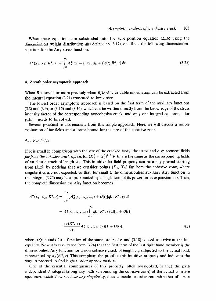
4. Zeroth order asymptotic approach

When R is small, or more precisely when RID ~ 1, valuable information can be extracted from the integral equation (3.21) truncated to low order.

The lowest order asymptotic approach is based on the first term of the auxiliary functions (3.8) and (3.9), or (3.15) and (3.16), which can be written directly from the knowledge of the stress intensity factor of the corresponding noncohesive crack, and only one integral equation - for Po(~) - needs to be solved.

Several practical results emanate from this simple approach. Here, we will discuss a simple evaluation of far fields and a lower bound for the size of the cohesive zone.

4.1. Far fields

If R is small in comparison with the size of the cracked body, the stress and displacement fields far from the cohesive crack tip, i.e. for (X~ + X2) 1/2 >> R, are the same as the corresponding fields of an elastic crack of length Ao. This intuitive far field property can be easily proved starting from (3.25) by noticing that we consider points (X1, X2) far from the cohesive zone, where singularities are not expected, so that, for small t, the dimensionless auxiliary Airy function in the integral (3.25) may be approximated by a single term of its power series expansion in t. Then, the complete dimensionless Airy function becomes

f o A*(xa, x2; R*, r) = [A*(xl, x2; ao) + O(t)]q(t; R*, r)dt

fo = A*(xl, x2; ao) q(t; R*, r)dt[1 + O(r)]

aN(R*, r)

O- R A~4(X1, X 2 ; ao)[1 + O(r)], (4.1)

where O(r) stands for a function of the same order of r, and (3.18) is used to arrive at the last equality. Now it is easy to see from (3.24) that the first term of the last right hand member is the dimensionless Airy function for a non-cohesive crack of length Ao subjected to the actual load, represented by aN(R*, r). This completes the proof of this intuitive property and indicates the way to proceed to find higher order approximations.

One of the essential consequences of this property, often overlooked, is that the path independent J integral (along any path surrounding the cohesive zone) of the actual cohesive specimen, which does not bear any sinoularity, does coincide to order zero with that of a non


cohesive specimen with a crack of length Ao. According to the definition of nominal stress intensity factor:

j _ KzI(aN, ao) K~N [1 E' [1 + O(r)] = ~ + O(r)]. (4.2)

Remark that the above relation between J and the nominal stress intensity factor does not imply the existence of an autonomous region for the cohesive crack (a region dominated by K~N), because it is based on a property of remote regions where the dominance of the singularity has already faded.

To show how the remote fields of the cohesive and non cohesive specimens approach each other, the complete solutions for stresses and displacements for the Dugdale model in the centre cracked panel - (2.28) and (2.30) - are compared in Fig. 4 with the solution for the non cohesive crack of length 2Ao subject to the same remote stress - (2.22) and (2.23) scaled by ar~/aR given by (2.29) - when the cohesive crack zone has extended by R = 0.1Ao.

(

t~ 1.0 " b

o x " 0 8

~ou) ...... . .~. ~ re

~ 0.4

~ ~R SOLUTION UJ

t~" . . . . . . . . . 0 th . O R D E R A P P R O X .

1 St. O R D E R A P P R O X .

O0 , I , I , I , I J

0 1 2 3 L,

R E L A T I V E D I S T A N C E , X /R

0.6

12.5

,,,k = b

. ~ 100 .......... ~"-~"~<'~'

Z 7.5 tu =E i , i (.)

5 . 0

---- 2.S ~ COMPLETE SOLUTION I • I - . . . . . . . . . 0 Ih . O R D E R A P P R O X .

r r , , j , ~ , , ;1~

0 0 -I0 -8 -6 -4 -2 0

R E L A T I V E D I S T A N C E , X / R

Fig. 4. Far field solutions for a cohesive Griffith crack (Ao = 10R): (a) Stresses. (b) Displacements.


4.2. Nearfields

The stress and displacement fields near the cohesive zone, when R ~ D, can be computed from the zeroth order asymptotic approach. For N = 0, the dimensionless auxiliary and density functions, according to (3.15), (3.16) and (3.20) are:

0"* E(~ - ~)r; a 0 + ~r] = floo(¢ - ~ ) - l / 2 r - 1 / 2 H ( ~ - (), (4.3)

w* [(~ - Or; ao + ~r] = 8R* floo(~ - ¢) x/2r- 1/2H(~ -- ¢), (4.4)

p(~; r, R*) = Po(~; R*) (4.5)

and the corresponding stresses and displacements along the crack line are:

a*(¢) = floo(¢ - O- '/ZPo(~; R*)H(~ - 0 d~, (4.6)

fo' w*(~: R * ) = 8R* floo(~ - ~)a/2Po(~; R*)H(~ - 0 d~, (4.7)

The load level may be characterized by the nominal stress intensity factor defined in (3.10), which may be rewritten in dimensionless form as

KI N /* 1 K*N -- ~ -- ~ floo | Po(~; R*)d~. (4.8)

x / / Z t , F do

The unknown function Po(O, defined for ~ in (0, 1), must be obtained as the solution of the 0th order approximation of the integral equation (3.21)

where the dependence of the solution Po(0 on R* is implicit in this equation and has been dropped from the notation. The solution depends on the material properties through the softening curve F* (w*), but it is size and specimen independent. In general, the integral equation (4.9) cannot be solved analytically and one has to resort to numerical procedures.

One interesting exception is again the Dugdale - or rectangular - softening model, where F*(w*) = 1 for w* < 1. In this case the solution of (4.9) is found to be

~-1 /2

P o ( 0 -- /~flO0

and the stresses (4.6), once given their dimensional form, are:

a22(X, 0) 2 RCOS_I( 1 _ R/X)X/2 for X i> R "

(4.10)

(4.11)


The crack opening w(X) is, from (4.7),

w(X) = 8Ra____~R 1 -- + -~ln -r---,1/2- for X ~< R (4.12) ~zE'

and the nominal stress intensity factor:

KIN = O ' R ~ . (4.13)

This solution is valid as long as the CTOD is less than the critical crack opening, i.e. for R ~< re/8 l~h. After this point, the cohesive zone travels in a selfsimilar state. Note, again, that all the solutions, for a given R, are shape independent. These results are formally the same one would get by considering a semi-infinite crack into an infinite body, as done by Rice [9] using the complex function formulation.

The above results for the Dugdale model are pictured in Fig. 5 and compared with the exact results for the centre cracked panel previously considered - (2.28) and (2.30) - when RID .= R/Ao = 0.1.

For softening behaviours other than Dugdale's, no closed form solution has been found so far. However, whatever the softening curves are, there are some common properties of near tip cohesive fields worth studying.

An essential aspect to consider for numerical formulations is the possibility of singular behaviour of the unknown function Po(0. This may be detected by relating Po(0 to the cohesive stress distribution, which may be performed analytically. Indeed, if we express that the right hand member of (4.9) is no more than the cohesive stress distribution a~oh(¢) we find the Volterra integral equation:

fo flO0( ~ -- ~)- 1/2p0(~ ) d~ = Crcoh(~), (4.14)

which may be inverted to give

trc°h(0+) 1 ~i d~ Po(O - 7 t f loo~ + r~flo----~o (( - 0 -1/2da (~)d~, (4.15)

which shows that Po(0 displays a (-1/2 singularity whenever there is a stress discontinuity at the initial crack tip (acoh(0 ÷) :~ 0). If the integral in (4.15) is interpreted in the sense of the theory of distributions, the result is easily extended to any stress discontinuity since at these points the stress derivative becomes a Dirac delta distribution. No other singularity of interest has been detected so far. Incidentally, the solution for the Dugdale case - (4.10) - is a particular case of (4.15).

As far as the physical solutions are concerned, the first aspect easily analyzed with the asymptotic formalism is that of the crack opening profile. Cohesive crack displacements near the end of the process zone are not like elastic cracks which display vertical tangent and behave as pl/2 (where p = 1 - 4, see Fig. 3). Instead, they display horizontal tangent and behave in general


A o x 0.8 v

- 0.6 ffl if) ul IIC p-

0.4 W >

<

02 n-

00

COMPLETE SOLUTION APPROX. . . . . . . . . 0 th. OROER ASYMPTOTIC

~ 1 . . . . . 1 St. ORDER ASYMPTOTIC APPROX.

a I , I , I , I , 2 4 6 8

R E L A T I V E D I S T A N C E , X/R

2O " ~ 1 1 ~ [ COMPLETE SOLUTION

. . . . . . . . 0 th. ORDER ASYMPTOTIC APPROX t]: - ~ . I st. ORDER ASYMPTOTIC APPROX.

,,= ~ ' - . .

¢.

,~ b L

-10 - B - 6 - 4 - 2 0

R E L A T I V E D I S T A N C E , X/R

Fig. 5. N e a r field solut ions for a cohes ive Griffith crack (A 0 = 10R) : (a) S t r e s s e s . (b) Displacements .

a s p3/2, as can be easily proven from (4.7). Indeed, if the density function Po(0 admits a Taylor's series development at ( = 1 one has, when p ~ 0:

w*(p) = l~3 R*flooPo(1)p3/2 + 0(p5/2). (4.16)

At the initial crack tip, the crack opening displacement (CTOD) is obtained by taking the limit of (4.7) when ~ approaches to 0, i.e.:

CTOD* = lira w*(~) = 8R*floo (1/2p0(() d ( ~ 0

(4.17)

and a more detailed analysis proves that, in general, the derivative of the crack opening at the initial crack tip diverges whenever there is a stress discontinuity (because of the singularity in Po(0). Such singularity does exist for any softening function until the CTOD reaches the critical crack opening value. For softening functions with a sudden stress drop, such as Dugdale's, the singularity is always present at the real crack (non-stress-transferring crack) tip.


A similar analysis may be performed for the stress profile. Since at the end of the process zone ((, ~ = 1) the crack opening is zero, the dimensionless stress must take the value 1 at this point. From (4.6) it is easily shown that the stress normal to the crack line is continuous at this point, but that its derivative is discontinuous. Indeed, for normally behaving softening functions (finite slope at the start of softening), the stress distribution at the left of the cohesive zone end has horizontal tangent, while at the right of this point the slope is - ~ .

Apart from the above morphological properties, there is an essential point providing the nexus between the near and far field properties. It is the J integral. Indeed, when paths completely surrounding the cohesive zone are considered, J is shown to be expressible in terms of the CTOD and the specific work supply defined in (2.2) as

J = Wr(CTOD), (4.18)

just by making the integration path shrink down to the upper and lower surfaces of the cohesive zone [9]. And since J is path independent, it must be equal to the far field expression for J - (4.2) - so that in the zeroth order approximation we have

K?N = Wv(CTOD) or K .2 = W*(CTOD), (4.19)

E'

where W* = We/Gr. From this result and (4.19) it is possible to derive a lower bound for R, the size of the cohesive zone. Dividing (4.17) by (4.8) one finds

_ 8 R * CTOD* ; x / ~ ((1/2), (4.20) KrN

o r

R* _(crov, 2 = 3 2 \ K*N /] ((~/2)-2, (4.21)

where ( f ( 0 ) stands for the po-weighted average of the function f ( 0 over the cohesive zone:

fo f(OPo (0 d( ( f (O) = ~ - - • (4.22)

f Po(O d( do

Substituting K * from (4.19) into (4.21) one gets

72 C T O D . 2 R* = ((1/2)- 2. (4.23)

32 W*(CTOD)

If Po(0 t> 0, for 0 ~< ( ~< 1, then ((1/2) < 1 and one arrives at the following lower bound theorem:


Zeroth Order Lower Bound Theorem for R. For a cohesive material and a general geometry under

proportional mode I loading, the size of the cohesive zone, when D -~ ~ , verifies,

rt CTOD .2 R* >~ 32 W* (CTOD)" (4.24)

In particular, when CTOD reaches the critical value we, the critical size of the cohesive zone verifies

R*/> ~ . . c , (4.25)

or, in dimensional form

2 E' Rc/> ~ wc G-Fv" (4.26)

Going back again to a cohesive crack with a softening function of Dugdale type, the CTOD (in the 0th order approximation) can be obtained from the displacement solution (4.12) when X = 0 , as

8 R a R CTOD = w(O) - roE' (4.27)

and the critical size of the cohesive zone is

71" 2 E' Rc = ~ wc ~ , (4.28)

where GF = aRw~. This result agrees with the lower bound given in (4.26).

5. First order asymptotic approach

When (R/D) 2 can be neglected in front of 1, one can go one step further by considering the first order asymptotic approach. Now, the auxiliary functions are truncated at the second term, and the density function also has two terms which are obtained by solving two integral equations; one corresponding to the 0th order and the second to first order terms in R/D.

Again, several practical results emanate from this approach; as the equivalent elastic crack theorem for far fields and a lower bound for the equivalent crack extension.

5.1. Far fields

The essential far field property of the first order approximation is that at points remote from the cohesive zone any field becomes coincident with the corresponding field of an effective (or equivalent) elastic crack subjected to the same load as the cohesive specimen.


To prove this property, we follow a procedure similar to that in Section 4.1 but we have to make the first order terms explicit. Hence, we start with a two term approximation of the dimensionless auxiliary Airy stress function, appearing in (3.25):

A~(xl - t, x2; ao + t) = A*(xl, X2; ao) + A*'(xl, x2; ao)t + O(t2), (5.1)

where O(t 2) means terms of the order of t 2 and A*'(xl, x2; ao) stands for

A,,(xl, x2; ao)=[ QA~i(x'l, x2; a) aA*(x'l, X2; a)q l (5.2)

The Airy stress function may then be expressed, according to (3.25), as

fo ;o A(xI, x2; R*, r) = A~(xl, x2; ao) q(t; R*, r)dt + A~'(xl, x2; ao) tq(t; R*, r)dt

+ O(r 2) q(t; R*, r)&, (5.3) do

or, taking into account (3.18) and (3.19),

A(xl, x2; R*, r) - ~rN(R*' r)[A~(xl, x2; ao) + A~'(xl, x2; ao)r(()(R*, r) + O(r2)], (5.4) O" R

where (()(R*, r) is the p-average of the relative position ~ over the fracture zone which, up to first order approximation, verifies:

fo ~p(~; R*, d~ r )

((>(R*, r),= = (()(R*, 0) + O(r), (5.5)

V p((; R*, r)d~

or, according to (3.20) and the definition (4.22)

~ (Po(~; R*) d( ((>(R*, 0):= = <~>o(g*), (5.6)

Po((; R*) d(

which finally leads to the first order expression for the Airy stress function:

A(xl, x2; R*, r) aN(R*, r)[A.(xl ' x2; ao) + A~'(xl, x2; ao)r<()o(R*) + O(r2)]. (5.7) O" R


Now, consider a virtual elastic specimen of the same geometry subject to the same load but with an elastic crack of reduced length ao + Aa. Let us suppose that Aa is of the same order as r and, consequently, Aa ~ 1. The corresponding Airy function is, in accordance with the definition of the auxiliary solution,

* Aa) - Avlrt(Xl, X2; ao, aN(R*,

r)A*(xl - Aa, x2; ao + Aa) (5.8) O" R

and using a two term expansion as in (5.1):

* A a ) - Avirt(X1, X2; ao, aN(R*, r)

O" R [AA*(X1, X2; ao) "1- A~'(x1, x2"~ a0)Aa + O(Aa2)]. (5.9)

A glance at (5.7) and (5.9) shows that the two Airy functions coincide up to first order if Aa is chosen to be the asymptotic equivalent crack extension Aao~ which, obviously, is first order in r and depends on the cohesive zone size R:

Aa~(R*) = r(()o(R*). (5.10)

Its absolute forms are, however, independent of the size:

A A ~ = R ( ( ) o ( R * ) or AA* AA~ - l c h - - R*(()o(R*) , (5.11)

which completes the proof of the

Far Field Equivalent Crack Extension Theorem. For a cohesive material and a general geometry under proportional mode I loading, every far field may be approximated, up to order R/D, by the corresponding field of a far field (FF) equivalent elastic crack of length Ao + AA~, subjected to the same load. The FF equivalent crack extension AA~ is given by (5.10) or (5.11).

To illustrate the interest of this equivalence, the stresses and displacements of this approximation are compared in Fig. 4 with the complete solution and with the 0th other solution for the centre cracked panel (with Dugdale softening) for a relative cohesive zone size r = R/Ao = 0.1. For this model, the FF equivalent crack extension is always equal to R/3 as is easily found using the solution for Po given in (4.10) to perform the integrals in (5.6).

A lower bound for the effective crack extension AAo~ can be derived in the same way as the lower bound for the extension of the cohesive zone, R. Working with the dimensionless expression in (5.11) and realizing that only terms O(R) are needed for this first order approach, R* can be approximated by (4.23) and then one finds

rC CTOD .2 (~)0 AA~ - 32 W*(CTOD) (~1/2)2, (5.12)

where the dependence of the po-averages on R* has been dropped from notation.


If cohesive stresses are monotonically increasing with x inside the cohesive zone, i.e. dtr/dx >1 0, then, from (4.15), P(O/> 0, and the Bunyakovsky-Schwarz inequality [8] may be used to find

( ( )o >~ (~z/2)o2. (5.13)

From this result this lower bound theorem follows:

Lower Bound Theorem for the FF Equivalent Crack Extension. For a cohesive material and a

general geometry under proportional mode I loading, the FF effective crack extension - up to order

R/D -, always verifies

~z CTOD .2 AA* /> . (5.14)

32 W~(CTOD)

In particular, when CTOD reaches the critical crack opening value %, the critical effective crack extension verifies

AA*~ 7> rCw*2 (5.15) 32 c ,

or, in dimensional form

/'C 2 E ' AA~oc >1- -Wc- - . (5.16)

32 GF

The critical effective crack extension for the Dugdale model is, from (5.11), AA~ = Re~3 or from (4.28)

2 E' (5.17) AA°°c = 2 -~wc Gr'

which satisfies (5.16).

5.2. Near fields

The stress and displacement fields near the cohesive zone, when (R/D) 2 can be neglected in comparison with 1, can be computed using the first order asymptotic approach. For N = 1, the dimensionless auxiliary and density functions are, according (3.15), (3.16) and (3.20)

a*(r/r; ao + (r) = rl-i/2r-i/2n(rl)[Qo((, rl) + QI((, q)r]

= (~ - ()-Z/2r-Z/2HOl){floo + [flol( + flzo(~ - ()]r}, (5.18)

w~(qr; ao + (r) = R*tll/2r- ~/2 H(-e)[Ro(( , ~) + RI((, ~/)r]

= 8R*(( - ~)~/2r-~/2n(-rl){floo + [flol( -½fllo(( - ~)]r}, (5.19)

p((; R*, r) = Po((; R*) + pl((; R*)r (5.20)

Asymptotic analysis o f a cohesive crack 175

and the corresponding stresses and displacements along the crack line are, to first order in r:

tr*(~; R*, r) = floo(~ - 0-1/2po((; R*)H(~ -- 0 d ( + r {floo(¢ - 0-1/2P1((; R*)

+ [flOl ~(¢ -- 0 - ' :2 + fl,o(~ - O'/2]P,(~; R*)}H(~ -- 0 d r , (5.21)

w*(~; R*, r) = 8R* ~oo(~ - ~)l/~po(~; R * ) H ( ~ - ~)d~ + r 8 R * {~oo(~ - ~)1/2P1(~; R*) d o

+ [flo~(~ - ~)1/2 _ ½fl~o(( - ¢)3/23Po(~; R*)}H(~ - 3)d(, (5.22)

where Po((; R*) and pa((; R*), defined for ~ in (0, 1), must satisfy the 1st order approximation of the integral equation (3.21) which, in view of (5.21) and (5.22), is now split into the two following size-independent integral equations:

(4.9), (5.23)

floo(~ - 0-1/2P~(0 d( = G(~, R*)8R* floo(~ - - ~)1/2p1(~) d~ + BI(~, R*), (5.24)

where the dependence on R* of the unknown functions is implicit in the equations and has been dropped from the notation, and

and

Bx(~; R*) = G(¢, R*)8R* [/3ol ~ -- ½fl,o(~ -- ~)](~ - ~),/2 Po(~)d~

+ I/~o1 ff +/~1o(¢ - 03(~ - 0 - 1 / 2 p o ( 0 dff.

Obviously - from (5.23) - Po(0 is the solution for the zero order approximation analysed in the previous section, and a single further linear integral equation has to be solved for Pl(~), (5.24), depending nonlinearly on the zeroth order solution.

In general, the Nth other asymptotic approach is reduced to solving a system of N + 1 integral equations; the first is the nonlinear integral equation (4.9) or (5.23) determining Po(0 and the remainder are a set of N linear integral equations, similar to (5.24), determining the functions p,(() - (n = 1, 2 . . . . . N) - where the functions B.(~; R*) depend only on the set {Po(0 . . . . , p,_l(()} of solutions of the lower order equations and on those ilk,, coefficients such that k + m ~< n. This formulation is material and specimen independent and is useful not only to obtain particular solutions, but also for an analysis of the asymptotic behaviour.


The solution of the system may be performed in a sequential way up to any order. Moreover, the function G(~, R*) as well as the kernels in the Volterra integrals are the same for all the integral equations of orders 1, 2, . . . , so the various orders differ only in the independent term. In a numerical algorithm this means that the stiffness matrix is the same, which greatly simplifies the finding of approximate solutions for order higher than 1. It is also worth pointing out that the stiffness matrix of the equations of higher order coincides with the tangent stiffness matrix of the zeroth order equation, so that if a Newton-Raphson method is used to solve (4.9), it is an easy matter to obtain the higher order solutions without having to generate new stiffness matrices.

The general case must be treated numerically. However, for the Dugdale or rectangular softening case, where F*(w*) = 1 for w* < 1, (5.24) is reduced to

floo(~ -- ~)-'/ZPl(~)d~ + [flol~ + fllO(~ - ~)](~ - ~)- X/ZPo(~) d~ = 0, (5.25)

where Po(0 was already obtained in (4.9). Solving (5.25) with the help of the inversion formula (4.15) (with the obvious change of Po(() by Pl(() and of acohe by the independent term of (5.25)) one arrives at

Pl(ff) = - fl01 q-fl10~1/2 __ 5v -~1/2, " / ~ (5.26) ~flo2o 4re

where the values of floo, flol, and fllO have been taken to correspond to the centre cracked infinite panel previously analyzed.

The corresponding stresses and displacements, up to first order in R/D, are, from (5.21) and (5.22):

G 2 2 ( X , 0) = G R for 0 ~< X ~< R, (5.27)

+ 3 X azz(X,O)=2anR[cos-'(l --Rf/z ~(~-- I)'/2~] for X~>R, (5.28)

w(X)= ~ 1 - - - + ~ l n l + ( 1 - X / R ) '/2 ~ - RJ OJ' (5.29)

for X ~< R. These results are plotted in Fig. 5 and compared with the exact results previously obtained, for the case r = R/Ao = 0.1.

Acknowledgements

The authors would like to thank Rosa M. Morera for careful preparation of the manuscript and Frlix Ustfiriz for his assistance in drawing Figs. 4 and 5. This research was sponsored by CICYT, Spain, under grants CE 89-0012 and PB 86-0494.


References

1. G.J. Barenblatt, Advances in Applied Mechanics 7 (1962) 55-125. 2. D.S. Dugdale, Journal of Mechanics and Physics of Solids 8 (1960) 100-104. 3. M. Elices and J. Planas, in Fracture Mechanics of Concrete Structures, L. Elfgren (ed.), Chapman and Hall (1989)

16-66. 4. J.N. Goodier, in Fracture, Vol. 2, H. Liebowitz (ed.), Academic Press (1968) 1~6. 5. A. Hillerborg, M. Modeer and P.E. Petersson, Cement and Concrete Research (1976) 773-782. 6. M.F. Kanninen, A.K. Mukherjee, A.R. Rosenfield and G.T. Hahn, in Mechanical Behaviour of Materials under

Dynamic Loads, Springer-Verlag (1968) 96-133. 7. A.S. Kobayashi, in Computational Methods in the Mechanics of Fracture, S.N. Atluri (ed.), North Holland (1986)

21-51. 8. S.G. Mikhlin, Integral Equations, Pergamon Press, Oxford (1964) 21-51. 9. J. Rice, in Fracture, Vol. 2, Academic Press (1968) 192-311.

Asymptotic analysis of a cohesive crack: 1. Theoretical background

Documents

Transcript of Asymptotic analysis of a cohesive crack: 1. Theoretical background