LINEAR DISCRETE MODELS WITH DIFFERENT

TIME SCALES

Eva Sanchez!, Rafael Bravo de la Parra2, Pierre Auger3

1Depto. Matematicas, E.T.S.I. Industriales, U.P.M., c/ Jose Gutierrez Abascal, 2, 28006Madrid, Spain.2 Depto. Matematicas, Univ. de Alcala, 28871 Alcala de Henares, Madrid, Spain.3 Univ. Claude Bernard-Lyon 1, 43 Boul. 11 novembre 1918, F-69622 Villeurbanne Cedex,France.

Aggregation of variables allows to approximate a large scale dynamical system (the micro-system)involving many variables into a reduced system (the macro-system) described by a few number ofglobal variables. Approximate aggregation can be performed when different time scales are involvedin the dynamics of the micro-system. Perturbation methods enable to approximate the largemicro-system by a macro-system going on at a slow time scale. Aggregation has been performed forsystems of ordinary differential equations in which time is a continuous variable. In this contribution,we extend aggregation methods to time-discrete models of population dynamics. Time discretemicro-models with two time scales are presented. We use perturbation methods to obtain a slowmacro-model. The asymptotic behaviours of the micro and macro-systems are characterized by themain eigenvalues and the associated eigenvectors. We compare the asymptotic behaviours of bothsystems which are shown to be similar to a certain order.

KEYWORDS Approximate aggregation of variables, population dynamics, perturbations, timescales, eigenvalues and eigenvectors analysis.

Ecological modelling deals with systems involving a large number of variables. Indeed, anecosystem is a set of interacting populations. Populations are composed of individuals ofdifferent ages or in different physiological stages. Individuals do perform several activities.For example, they search for food of different types, they take care of youngs a.s.o.Furthermore, individuals move and can go to different sites. Thus, populations are dividedinto various sub-populations corresponding to ages, stages, individual states or activities,phenotypes, genotypes, spatial patches etc. When modelling ecological systems, we arefaced to a complexity of structures of populations.

A first solution is to build a mathematical model describing the real system in details.This leads to a family of models involving a very large number of variables. The

Acta Biotheoretica 43: 465-479, 1995.© 1995Kluwer Academic Publishers. Printed in the Netherlands.

complexity of the system is included in the model. Few mathematical techniques areavailable for these models which are difficult to handle. Mostly, one must use computersimulations. Robustness of the solutions with respect to parameters and initial conditionsis in general unknown. If one wants to take into account all aspects in the same model, thisleads to a complex model involving a too large number of coupled variables.

On the contrary, many models of ecological communities only deal with a few numberof variables. This means that the structure of the populations is often ignored. Thepopulations are considered as entities and are described by a single variable, for examplethe total population or density. This simplification implies that the effect of the internalstructure of the population is neglected. It is an assumption corresponding to anapproximation of the total system by a reduced system which has to be checked. However,in most cases, simplified models are used and few arguments are given to justify thesemodels.

Our approach is halfway between these two approaches. We intend to take into accountthe existence of different time scales to proceed to approximations which allow to substituteto a large scale system a reduced model. Thus, we start with a large scale model but, weuse methods to reduce it into a simple aggregated version. Perturbation and averagingmethods allow to perform these approximations in a rigorous way and lead to asimplification of the initial system into a reduced system which is described by few globalvariables at a slow time scale. Moreover, these approximations not only provide a simpleversion but also, interaction terms between the fast and slow dynamics which haveimportant ecological significances.

The simplified model is an approximation of the initial system and is obtained by anapproximate aggregation of variables. In previous contributions (Auger, 1989; Auger &Benoit, 1993; Auger & Roussarie, 1994), we realized aggregations of systems of ordinarydifferential equations with different time scales. In these models, time was a continuous realvariable. The aim of this work is to perform approximate aggregation in time discretemodels. A first contribution can be found in Bravo et aL (to appear) in which we describedthe growth of an age and patch structured population.

Time discrete models are widely used in population dynamics and many ecologicalmodels involve a discrete time. For example, the Leslie model describes an age structuredpopulation at discrete times (Caswell, 1989; Logofet, 1993). The Nicholson-Bailey modeldescribes the dynamics of a host-parasitoid system of insect populations (Edelstein-Keshet,1988). Time discrete models are particulary well adapted for the study of the life cycle ofdifferent populations. When the reproduction occurs periodically each year, time discretemodels can provide the density of the populations at consecutive generations.

Most of the usual time discrete models describe the dynamics of the total density ofpopulation. However, individuals migrate and go to different patches, they also performdifferent types of activity (such as search of parasites or preys, attack, etc.) at a fast timescale in comparison to age or stage changes or else to the overall growth of the populationsto which they belong. In order to take into account the patch dynamics and the individualbehaviour, it is necessary to subdivide the populations into several subpopulations associatedto spatial patches or to individual states. Then, one must start with a time discrete modelwhich describes the dynamics of many subpopulations.

In this article, we present different time discrete models with subpopulations dynamicsat different time scales. We use aggregation methods to condense this large scale model intoa reduced version. We prove that the asymptotic behaviours of the initial large scale system

and of the reduced approximated system are close enough when the two time scales aresufficiently different. Following (Bravo et al., to appear) we show that the main eigenvaluesand the associated eigenvectors of initial and reduced systems are of the same order.

We suppose a stage-structured population, then classified into groups or stages basedon the structure of the life cycle. Moreover, each of these groups is divided into severalsubgroups, that we consider as being different spatial patches, different individual activitiesor any other character that could change the life cycle parameters.

Our study is general. Thus, we do not state in detail the nature of the subpopulationswhich can correspond to patches, individual states or any other types of subpopulations. Weconsider a set of q populations (or groups) which are subdivided into subpopulations (orsubgroups). Let xl be the density of subpopulation k of population j at time n,j = 1,...,qand k = 1,...,Ni. N is the number of subpopulations of population j and N is the totalnumber of variables, i.e. of subpopulations, N = N1 +...+ N'l. We use vector Xn to describethe total population at time n. This vector is a set of population vectors x~describing theinternal structure of each subpopulations as follows:

{.;1 -q T -j jl iNiXn = \xn,···,xn) where xn = (rn '···'X'n )

and (*,...,*l denotes transposition.In the evolution of this population we distinguish between two different dynamics, a

slow one and a fast one.The slow dynamics, for a certain fixed projection interval, is represented by a non-

negative projection matrix M, that in this context is usually called Leftkovitch matrix. Misdivided into blocks Mij' 1 s 4j s q,

Mll M12 M1q

M=M21 M22 M2q

...Mq1 Mq2 Mqq

being Mij of dimensions N x N and representing the rates of transference of individualsfrom the subgroups of group j to the subgroups of group i.

The fast dynamics is, for every group 4j = 1,...,q, internal, conservative of the totalnumber of individuals and with an asymptotically stable distribution among the subgroups.

For every group j, the fast dynamics, considering a fixed projection interval, small incomparison with that chosen for the slow dynamics, is represented by a projection matrixPj' which is a regular stochastic matrix of dimensions N x N. The matrix P that representsthe fast dynamics for the whole population is then

P = diag{P v...'pq}

Every matrix Pj has an asymptotically stable probability distribution Vj that verifies thefollowing properties:

T - T· -where Pj is the transpose of Pj' 1j = (1,...,1) , (N'x1) and < Vj' 1j >= 1. We define

Pj = ym pf •• (V jl···lv j)•••••• co

where pJ is the kth power of the matrix Pi"- - - k -We denote diag{P l""'p q} by P, and so we have limk__ P •• P.

Though in the continuous case it is immediate to include two different time scales, (seeAuger, 1989), there is not a direct way to do so in the discrete case. In our model we haveto combine two projection matrices whose associated projection intervals of which onemuch longer than the other. To avoid this problem we propose two qualitatively similarmodels which can prove to be a good approximate aggregation.

In the first model we use as projection interval the one associated to the fast dynamics,that is, to the matrix P. We need, therefore, to approximate the effect of matrix M over aprojection interval much shorter than its own. For that we use matrix

where E > 0 and little enough.We could think that M(E) makes M act in proportion E, as little as we want, and let

variables unchanged in proportion 1 - E. From a mathematical point of view the followingproperty of M( E) reflects the fact that we have approximately translated the dynamics ofM to the time scale of P:

If M has a dominant eigenvalue A. with an associated eigenvector V, then M(E) has E1.+ (l-E) as strictly dominant eigenvalue and v is also its associated eigenvector.

That implies that dynamics associated to M and M(E) have the same asymptoticallystable stage distribution but M has a much greater growth rate than M(E) because E1. + (1- E) is closer to 1 than A..

The first model consist of the following system of linear difference equations

In the second model the projection interval coincides with that of the slow dynamics, theone associated to matrix M. And so, we need to approximate the effect of matrix P over aprojection interval a number times longer than its own. We suppose in that case that P hasoperated such a number of times, that is, we use matrix pl, where k is a big enough integer.

In that way our second model consist in the following system of linear differenceequations:

3. AGGREGATION OF MODELXn+1 = M(e)PXn

In this and the next section we approximate a general system of N variables, thosecorresponding to the subgroups, by an aggregated system of q variables and those associatedto the groups. We shall prove that the general and aggregated system exhibit a similarasymptotic behaviour; to be more precise, that the elements defining the asymptotic

behaviour of both systems, dominant eigenvalues and eigenvectors, coincide to a certaindegree.

Beginning with the general system (1) and following the notation of the former sectionwe define the global variables

NiXi "" r ilc . 1 (3)n LJ xn ' } "" ,•••,q

1c=1

that indicate the total number of individuals in every group.'TI!.osenew variables could be obtained from vector Xn multiplying by matrix U =

T -Tdiag{11 ,.••,1q }

(xnl, ..., xn'l)T = UXn (4)

If in the general system (1) we multiply by matrix U

UXn+1 = U (M(e}p) Xn

we get the global variables in the first member but we do not get an autonomous systemon these variables.

If the system (5) were autonomous on the global variables, we would have obtained anexample of what it is called perfect aggregation, see (Iwasa ~t aL, 1987), that is onlypossible in very particular cases.

To avoid this problem we consider the following system instead of system (5)

where we suppose that, before aggregating, the subgroups variables have reached the stabledistributions associated to the fast dynamics.

To describe the so-called aggregated system we need to define a new matrix

Pc"" diag{vl' ...'vq}

If we have a vector belonging to R+q, that indi~tes the total number of individuals includedin the different groups, and we multiply it by Pc' we will obtain a vector belonging to R+Nthat would give how these individuals would be divided in the subgroups depending on thestable distributions of the fast dynamics.

In the following Lemma we state the properties of the matrices P, P, P co and U that wewill use frequently throughout the paper.

Lemma 3.1. The matrices P, P, Pc' and U verify the following identities:

a) PP = PP ""PP ""P

b)PPc""PPc=Pc- -

c) UP = U; UPc = Iq; PcU=P

The system (6) could be written as follows

UXn+1= UM(e}p JUXJ

and denoting the new variables UXn by Yn, we obtain

Yn+1= UM(e}p In

- -UM(E)P c = U(EM + (l-E)IN)Pc = E(UMP J + (l-E)Iq

- - - -and making M = UMPc and M(E) = EM + (l-E)Iq' the aggregated system presents thenext simple form

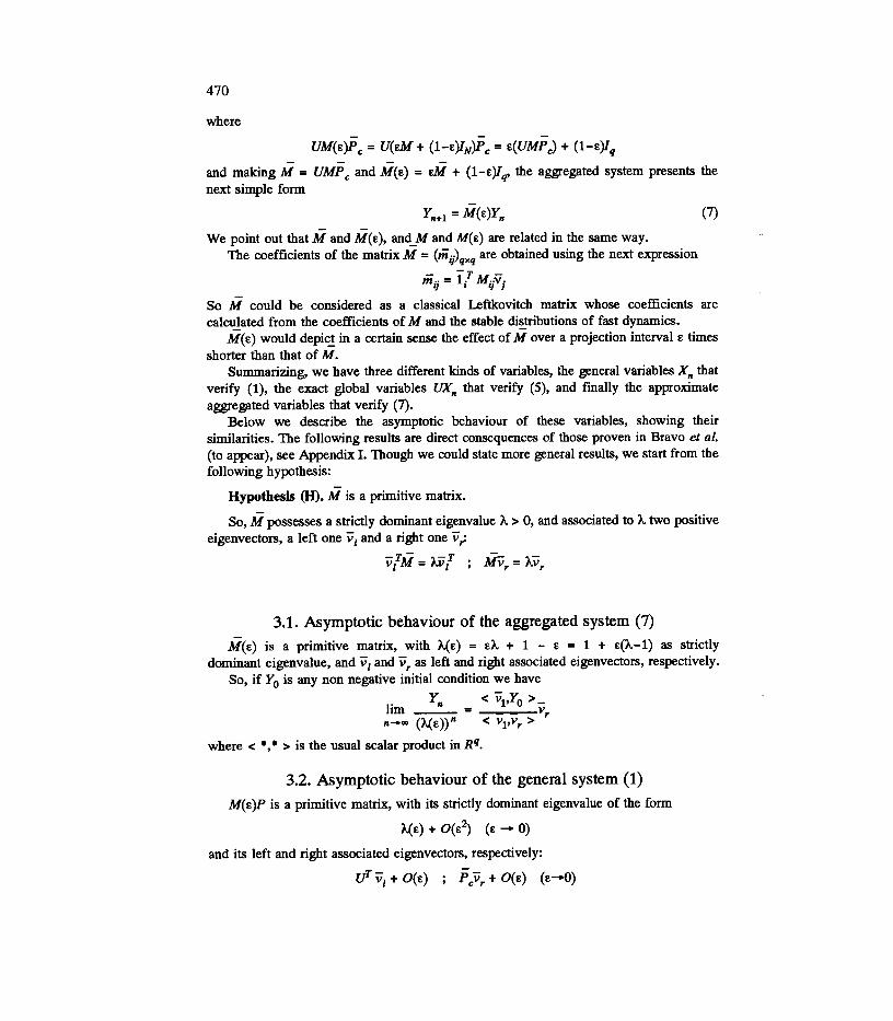
Yn+1 = M(E)Yn (7)- -

We point out that M and M(E), and_M and M(E) are related in the same way.The coefficients of the matrix M = (iii;)qxq are obtained using the next expression

- -TM-m;j = 1; ;jVj

So M could be considered as a classical Leftkovitch matrix whose coefficients arecalculated from the coefficients of M and the stable di~tributions of fast dynamics.

M(E) would depi~ in a certain sense the effect of M over a projection interval E timesshorter than that of M.

Summarizing, we have three different kinds of variables, the general variables Xn thatverify (1), the exact global variables UXn that verify (5), and finally the approximateaggregated variables that verify (7).

Below we describe the asymptotic behaviour of these variables, showing theirsimilarities. The following results are direct consequences of those proven in Bravo et ai.(to appear), see Appendix I. Though we could state more general results, we start from thefollowing hypothesis:

Hypothesis (II). M is a primitive matrix.

So, M possesses a strictly dominant eigenvalue A > 0, and associated to A two positiveeigenvectors, a left one v, and a right one v,:

v{if = AV{ ; iiv, = AV,

3.1. Asymptotic behaviour of the aggregated system (7)M(E) is a primitive matrix, with A.(E) = EA + 1 - E = 1 + E(A-1) as strictly

dominant eigenvalue, and v, and v, as left and right associated eigenvectors, respectively.So, if Yo is any non negative initial condition we have

. Yn < vl'Yo >-hm '" -v,n •..• oo (A.(E»n < vl'v, >

where < .,. > is the usual scalar product in Rq.

3.2. Asymptotic behaviour of the general system (1)M( E)P is a primitive matrix, with its strictly dominant eigenvalue of the form

A.(E) + 0(E2) (E ...• 0)

and its left and right associated eigenvectors, respectively:

UTvl + O(E) ; Pcv, + O(E) (E...• O)

Then, if Xo is any non negative initial condition we obtain

. Xn < ulV1+0(E),xo >hm "" __ -- __ --- (PCVy+O(E))n...•~oo(A.(E)+0(E2))n < UT¢l+O(E)'cVy+O(E) >

< vpUXo > -""----PCvy + O(E)< VpVR >

4. AGGREGATION OF MODELXn+1 = MpkXnThe results of last section that allow approximate aggregation of the system Xn+1 ""

M(E)PXn were based upon considering the matrix M(E)P ""P + E(M-l)P as an analyticalperturbation of the matrix P, see Bravo et aL (to appear). In this section the resultsconcerning approximation will be deduced from the identities

Hm pk "" P Mpk "" MP + M(pk_p)k ...•oo

that let us consider the matrix Mpk as a perturbation of matrix MPStarting with the general system (2), which we will call perturbed system, we define the

so-called non-perturbed system-

Xn+1""MPXn (8)

This system admits the interpretation of being an approximation of (2) in which the lastdynamics has reached its stable distributions.

In order to build an aggregated system we define the global variables xj as in (3) and(4), and we verify that

UXn+1 "" U M pk Xn

is again a non-autonomous system on these global variables.Nevertheless, if we aggregate variables in the non-perturbed system (8) we obtain

- -UXn+1 = U M P Xn = U M Pc U Xn- -

and making Yn = UXn and M = UMP co following the notation of the last section, we get thenext aggregated system:

We could remark that the non-perturbed system (8) is one of those few exceptional systemsthat are susceptible of being perfectly aggregated.

The rest of the section is devoted to the development of similar results to those provenin Section 3 about the asymptotic behaviour of ~e diffe.!ent treated systems. We start withrelating the spectral properties of the matrices MP and M, associated to the systems (8) and

(9), and later, using the m...!itrixperturbation theory, we will compare the asymptoticelements of the matrices MP and Mpk, what will yield the relation between systems (8)~~ -

We summarize in the next theorem the spectral relations between matrices MP and Mthat we will use below.

- -Theorem 4.1. The matrices MP and M verify:

a) det(AIN - MP) = )..N-q det(AIq - ii).b) If Iir ••0 is a right eige"Y.ector of MP associated to the eigenvalue ).. •• 0, then Uiir ••

o is a right eigenvector of M associated also to A.-

c) Ifvr •• 0 is a right eigenvector of M associated to the eigenvalue).. •• 0, then MP c vr•• 0 is a right eigenvector associated to the same eigenvalue A.

d) If iii •• 0 is a left eigenvector of MP associated to the eigenvalue ).. ~ 0, then thereexists VI E Rq - (OJ such that iii = UT v, and VI is a left eigenvector of M associated to).. too.

e) If VI •• 0 is a left eige!!:vector of M associated to the eigenvalue).. •• 0, then UTVI ••o is a left eigenvector of MP associated also to A.

Proof. a) P is a projector and so we could write

Jl!V = ker P @ImPThen we b~ld a basis of Jl!V starting witl.!..any basis of ker P and adding the column vectorsof matrix Pc' that form a basis of Im P. Let K.!?e the matrix of dimensions N x (N -q)whose columns are the_vectors in the basis ofker P. We now find the matrix representation,K, of the operator MP respect to the basis first defined. K should verify the followingidentity:

as MPK = 0, decomposing K into appropriate blocks, we have

(OIMPPo) • (KIPO> (: ~l

and multiplying on the left by U: - -UMPc = UKA+UPcB

and then follows that

det(A.IN-MP) '" det(A.IN-K) '" AN-qdet(A.Iq-M)

b)i4, •• 0 v~rifies MPIi, '" A.Ii, •• o.As MPIi, '" MP cVii, •• 0, then Vii, •• o. Moreover

MUU, '" UMPcUU, '" UMPu, '" AUU,

c) va:.." 0 verifies MVL", AV," o.As UMPcv, •• 0, then MPcv, •• o. Also

MPMPcv, '" MPcUMPcv, '" MPcMv, '" AMPcv,

d) iii" 0 verifies lit MP = A.lit.

As the first N1 columns of P are identical, and so happen to th~ next N2 columns, and soon, we have the same identities among the columns of lit MP and therefore among thecomponents of lirFrom that we deduce that there exists a vector VI E Rq - {OJ such that

-TU - T d 1 -T - T-VI "'"I an a so VI "'"I Pc

-T- -T - -T -- -T- -TVI M '" VI UMPc '" "I MPPc '" A"I Pc '" AVI

e) VI •• 0 verifies vt M = Avt •• O.So UTVI" 0 and

(UTvl)TMP '" v{UMPcU '" AV{U '" A(UTvl)T.

We begin now the study of the spectral relations between the matrices MP and Mpk,having in mind that Mpk could be considered a perturbation of MP:

Mpk '" MP+M(pk_P) '" MP+M(P_p)k

As every matrix Pi' i '" 1,...,q is a regular stochastic matrix of dimensions Jt x Jt, we couldorder their eigenvalues according to decreasing modulus in the following way:

1 2 Ni

Ai '" 1 > IAil~···~IAi IIf we do the same with the matrix P we should obtain

Al '" ... '" Aq '" 1>IAq+ll~ ..·~IANI

IAq+1 I '" max IA~I; i '" 1, ... ,qThe next proposition allows to fmd a bound of the perturbation.

Proposition 3.2. If I * I is any consistent norm in the space !MNxN of N x N matrices,then for every a. > IAq+11 it is verified that

Proof. See Appendix n.Before stating the asymptotic behaviours of the different mentioned systems, we make

the same hypothesis proposed in Section 3.

Hypothesis (8). M is a primitive matrix.

Let A > 0 be the strictly dominant eigenvalue of M, and vI and vr its associated left andright eigenvectors, respectively. We then have that, given any non-negative initial conditionYo, the aggregated system (9) verifies

Yn <vl'Yo>lim _ = vrn-oo An <V1,Vr>

Proposition 4.3. The non perturbed system (8), given any non-negative initial condition Xoverifies tluzt

XnJim _ =n _00 An

Proof. From Theorem 4.1 we deduce that

<UTvl'XO> -T- MPcvr

<u vl,MPcvr>

Xnlim_ =n _00 An

<VI'UXo>= --- --MPcvr<vI'UMPcvr>

<v1,UXO> --= ---....,,--- M Pc Vr

<V1,AVr>and that yields (10).

Proposition 4.4. The matrix Mpk has a strictly dominant eigenvalueT - k -<U v1,M(P-P) MPcvr>Itk '" A + -_--- + o(a2k)

<UTV1,MPcvr>

= A + O(ak)

and associated to Itk there exist a left and a right eigenvectors that could be written in thefollowing form, respectively

MPcVd + O(a~ (non-negative)

Proof. Immediate consequence of the Theorem in Appendix n.Theorem 4.5. Let system (2) verify (8). Then, given any non negative initial condition

Xo the system (2) verifies

and that yields (11).We should notice that the exact global variables verifies

. UXn <v1,UXo> 1 - khm ----- "" - __ - "r" UMPcvr+O(a )

n _00 (A,+O(ak))n <v1,Vr> '"

<vl'UXo> k"" - vr+O(a )<Vl'Vr>

Our general results allow for different applications. For example, it is possible to modela patch and age structured population, or else a patch structured community. Age structuredpopulations are commonly described by a Leslie matrix. When individuals go to differentspatial patches, one must also consider the spatial distributions of individuals among thedifferent sites. If patch migration takes place at a fast time scale with respect to agechanges, one can describe a patch and age structured population (see Bravo et aI., toappear).

It has been shown that spatial heterogeneity can playa very important role regardingthe stability of ecological communities (Hassel et aL, 1991). This was shown in a time andspace discrete version of the host-parasitoid Nicholson-Bailey model. Although the onepatch model is always unstable, computer simulations have shown that the spatial versionbecomes stable when the size n of the 2D array of (nxn) patches is large enough. Thisresult shows that the spatial dynamics can have important consequences for the dynamicsand stability of the community.

Our method allows to get the simplified aggregated model and also, to obtain therelationships between the parameters of the aggregated model and the parameters whichcontrol the fast dynamics. For example, in the patch and age structured population, theaggregated model is a classical Leslie matrix in which the overall fecundities and agingrates are expressed in terms of the spatial distributions of individuals on the differentpatches. Thus, a change in the spatial distribution has an effect on the aggregated Lesliematrix which can be calculated.

Facing local unfavourable situations and in order to avoid extinction, two main strategiescan be developed, either migration to find a better site or prolonged diapause to wait fora better context in the future. There are two alternate strategies. The Leslie model with fastpatch dynamics is a good tool for estimating the advantages of these two differentstrategies. We are now on the point to confront our model to experimental data relating toan insect population (the chestnut weevil) (Menu, 1993; Debouzie et aL, 1993).

In the future we also intend to use our general methods given here for the study of patchstructured communities. For example, we plan to model a patch structured host-parasitoidcommunity. An interesting problem is to check if one can obtain similar results than in thecell automaton spatial model of a Nicholson-Bailey model (Hassel et ai., 1991).

Auger, P. (1989). Dynamics and Thermodynamics in Hierarchically Organized Systems. Applicationsin Physics, Biology and Economics. Oxford, Pergamon Press.

Auger, P. and E. Benoit (1993). A Prey-predator model in a multipatch environment with differenttime scales. Jour. BioI. Systems 1: 187-197.

Auger, P. and R Roussarie (1994). Complex ecological models with simple dynamics: Fromindividuals to populations. Acta Biotheoretica 42: 111-136.

Baumgartel, H. (1985). Analytic Perturbation Theory for Matrices and Operators. Basel, BirkhauserVerlag.

Bravo, R, P. Auger and E. Sanchez. (to appear). Aggregation methods in discrete models. J. BioI. Sys.Caswell, H. (1989). Matrix Population Models. Sunderland, Sinauer Associates Inc.Debouzie, D., A Heizmann and L Humblot (1993). A statistical analysis of multiple scales in insect

populations. A case study: The chestnut weevil Curculio Elephas. J. BioI. Systems 1: 239-255.Edelstein-Keshet, L. (1988). Mathematical Models in Biology. Random House (1988).Hassel, M.P., H.N. Comins and R.M. May (1991). Spatial structure and chaos in insect population

dynamics. Nature 353: 255-258.Horn, R.A and C.A Johnson (1985). Matrix Analysis. Cambridge, Cambridge Dniv. Press.Iwasa, Y., V. Andreasen and S.A Levin (1987). Aggregation in Model Ecosystems. (I) Perfect

Aggregation. EcoI. Modelling 37: 287-302.Kato, T. (1980). Perturbation Theory for linear Operators. Berlin, Springer Verlag.Logofet, D.O. (1993). Matrices and Graphs. Stability Problems in Mathematical Ecology. CRC Press.Menu, F. (1993). Strategies of emergence in the chestnut weevil Curculio Elephas (Coleoptera:

Curculionidae). Oecologia 96: 383-390.Stewart, G.W. and J. I-Guang Sun (1990). Matrix Perturbation Theory. Academic Press.

We present in this appendix a general result developed in Bravo et aL (to appear), thatimplies the asymptotic results of Section 3. (See Baumgartel, 1985; Horn & Johnson, 1985;Kato, 1980).

We follow the notation of Sections 2 and 3.We have the following general difference equations system depending on the little

parameter e:

Xn+1(e) =A(e)xie) (12)

Every matrix Ajie) has dimensions N x ~ and depends holomorphically on e. So

A(e) = A(O) + EA'(O) + ...

We make the next two hypothesis on A( e):

Hypothesis (HI). A(O) has the same structure of matrix P, that is, AjiO) = ° wheneverj ••k, and AiO) is a regular stochastic matrix, j,k = 1,...,q.

- -Hypothesis (H2). Matrix P A'(O) P has a simple nonzero eigenvalue I.l. whose real part

is strictly greater than the real parts of the rest of eigenvalues.- -

Let v be an eigenvector of P A' (0)P associated to I.l.. Let- -

B(e) = U A(e)Pc = Iq + eU A'(O)pc + ...

and so the aggregated system is

Yn+1(e) = B(e)Yie)

Theorem. Let system (12) verify (H1) and (H2). Then, there exist II > °such that for everye > 0, e < ll, we have:

a) A( e) has a simple eigenvalue whose modulus is strictly dominant and that admits thefollowing expression:

A..nax(e) = 1+ el.l. + 0(e2) , (e - 0)

Associated to this eigenvalue there exist a unique eigenvector of A( e) that could be writtenas follows:

x(e) = v + O(e) , (e - 0)

b) B( e) has a simple eigenvalue whose modulus is strictly dominant and that admits thefollowing expansion:

I.l.max(e) = 1 + el.l. + 0(e2) , (e - 0)

Associated to this eigenvalue there exist the next eigenvector of B(e):

)/(e) = UV + O(e) , (e - 0)

Proof of Proposition 3.2.

As P is the projector over the eigenspace of P associated to the eigenvalue 1 we have

JtI = ImP ® ker P

(P - P>unP = 0 ; (P - P\erP = P

We then conclude that the eigenvalues of P-P ordered by decreasing modulus could bewritten as follows:

Next, we apply the following known result relating the norms and the spectral radius of amatrix:

For every A belonging to the space Mnxn of n x n mtltrices and every I; > 0 there existsa consistent norm 11*1. in Mnxn such that p(A) ~ 11.41. < I; + p(A), being p(A) thespectral radius of A.

From (13) we have p(P-P) = 1A.q+ll and from the last result we deduce that for everya> lA.q+ll we could find a consistent norm U*lla such that

HP -Plla < a

As any two norms in Mnxn are equivalents we have for any norm 11*. in Mnxn and any k= 1,2,... that there exists C > 0 such that

I~ -PI ~ npk -Plla

lim IIMpk-MPIIk-oo ak

'" UMIC lim (IIP-halk '" 0k-oo a

Below we state the main result about matrix perturbation that it is applied in Section 4, see(Stewart, 1990).

Theorem. Let A. be a simple eigenvalue of n x n mtltrix A, with left and righteigenvectors Xl and x" respectively. Let A = A + E be a perturbation of mtltrix A, and 11*11any consistent norm in Mnxn• Then there exists a unique eigenvalue);'. of A such that

xTEx).. '" A. + _l__ r + O(lIEU2)

-T-Xl xr

Moreover, associated to );'.there exist left and right eigenvectors fl and f" respectively,such that

....X I = Xl + O(IIEIO

....X r = xr + O(lIEIO

The eigenvalue);. is the unique eigenvalue of A close to A. whenever lIE II is little enough.In our application of that result we will use that if A. is strictly dominant so will be ).'.forlittle lIEU.