AVACS – Automatic Verification and Analysis of

Complex Systems

REPORTSof SFB/TR 14 AVACS

Editors: Board of SFB/TR 14 AVACS

Exact State Set Representations in theVerification of Linear Hybrid Systems

with Large Discrete State Space

byWerner Damm Stefan Disch Hardi HungarSwen Jacobs Jun Pang Florian Pigorsch

Christoph Scholl Uwe Waldmann Boris Wirtz

AVACS Technical Report No. 21June 2007

ISSN: 1860-9821

Publisher: Sonderforschungsbereich/Transregio 14 AVACS(Automatic Verification and Analysis of Complex Systems)

Editors: Bernd Becker, Werner Damm, Martin Franzle, Ernst-Rudiger Olderog,Andreas Podelski, Reinhard Wilhelm

ATRs (AVACS Technical Reports) are freely downloadable from www.avacs.org

Copyright c© June 2007 by the author(s)

Author(s) contact: Werner Damm (wd@avacs.org).

Exact State Set Representations in the

Verification of Linear Hybrid Systems

with Large Discrete State Space

Werner Damm2,3, Stefan Disch1, Hardi Hungar3, Swen Jacobs4, Jun Pang2,Florian Pigorsch1, Christoph Scholl1, Uwe Waldmann4, and Boris Wirtz2

1 Albert-Ludwigs-Universitat FreiburgGeorges-Kohler-Allee 51, 79110 Freiburg, Germany

2 Carl von Ossietzky Universitat OldenburgAmmerlander Heerstraße 114-118, 26111 Oldenburg, Germany

3 OFFIS e.V., Escherweg 2, 26121 Oldenburg, Germany4 Max-Planck-Institut fur Informatik

Stuhlsatzenhausweg 85, 66123 Saarbrucken, Germany

Abstract. We propose algorithms significantly extending the limits formaintaining exact representations in the verification of linear hybridsystems with large discrete state spaces. We use AND-Inverter Graphs(AIGs) extended with linear constraints (LinAIGs) as symbolic represen-tation of the hybrid state space, and show how methods for maintainingcompactness of AIGs can be lifted to support model-checking of linearhybrid systems with large discrete state spaces. This builds on a novelapproach for eliminating sets of redundant constraints in such rich hy-brid state representations by a suitable exploitation of the capabilities ofSMT solvers, which is of independent value beyond the application con-text studied in this paper. We used a benchmark derived from an Airbusflap control system (containing 220 discrete states) to demonstrate therelevance of the approach.

1 Introduction

We target the verification of safety properties for embedded control applicationsin the transportation domain. Typical for such applications is a ratio of between1:5 to 1:10 between the core control algorithms and diagnostic and fault-tolerancemeasures integrated into the controller, leading to a blow up of the discrete statespace against pure control applications often reaching some 106 discrete states.As an example, we analyze a model derived from an Airbus flap controller [13],which on top of its control-loop for flap extraction and retraction is performingenvelope protection to prevent loads on flaps possibly causing physical ruptures,and offers extensive monitoring of the health of its sub-systems to e. g. react onloss of hydraulic pressure, rupture of the transmission shaft, or hardware fail-ures. To prove safety of such controllers, we must combine methods for analyzingthe pure control part (typically using linear dynamics for design models servingas reference for subsequent implementation steps) with state-space explorationmethods dealing with large discrete state spaces. Such applications are out of

reach for existing hybrid verification tools such as CheckMate [26], PHAVer [11],HyTech [15], d/dt [5]: while their strength rests in being able to address complexdynamics, they do not scale in the discrete dimension, since modes – the only dis-crete states considered – are represented explicitly when performing reachabilityanalysis. On the other hand, hardware verification tools such as SMV [20] andVIS [27] scale to extremely large discrete systems, but clearly fail to be applica-ble to systems with continuous dynamics. To achieve a compact representationof such hybrid state-spaces, we enrich AND-Inverter Graphs (AIGs) with linearconstraints. Previous work [23] demonstrated advantages of AIGs over BDDs forrepresenting large discrete state-spaces compactly, due to their higher robust-ness in handling broad classes of Boolean functions in exhaustive state-spaceexploration. We lift methods such as test vector generation and SAT checking todetect equivalent (and thus redundant) nodes to the LinAIG level, providing asuite of heuristics including precise checks for equivalent LinAIG nodes using theSMT solver HySAT [10]. Moreover, we provide efficient methods for detectingand eliminating redundant linear constraints from our LinAIG representationswhich are basically arbitrary boolean combinations of boolean variables and lin-ear constraints. This extends results for eliminating redundant linear constraintsfrom convex polyhedra used by Wang [28] and Frehse [11]. Our approach can beapplied to perform backward reachability both for discrete time models (suchas reference models for embedded controller implementation) and linear hybridautomata enriched with large discrete state spaces. In the latter case, we exploitthe fact that the number of modes of a single controller is typically small (inthe order of tens of modes) – this allows us to co-factor the LinAIG represen-tation along modes. For each mode, we use the Loos-Weispfenning quantifierelimination technique for backward evaluation of the symbolic state-space rep-resentation along continuous flows. We counteract a worst-case quadratic blowup of linear constraints by tightly integrating redundancy elimination into thequantifier elimination process. Jointly, the presented techniques allow to achievepreciseness while maintaining sufficiently compact representations for the tar-geted application class.

This paper significantly extends our previous work [7] in adding quantifierelimination and redundancy elimination. The introduction of quantifier elimina-tion was originally motivated by the wish to reduce the diameter of discrete timemodels. In allowing to fold the effect of large sequences of discretized flows intoa single substitution, we accelerate hybrid system verification. This is differentfrom the acceleration by folding hybrid control loops as in [6] which is performedin the world of few discrete states.

The presented methods are orthogonal to and may in the future be combinedwith abstraction techniques (such as bounding the degree of precision or loosen-ing constraints as in [11]), incorporating robustness [12, 8] or slackness [1, 2] inmodels allowing precise abstractions by finite grids under robustness respectivelyslackness assumptions, counter-example guided abstraction refinement as in [24,17, 25] and techniques such as hybridization [4] for approximate linearization ofricher dynamics.

The paper is organized as follows: Sections 2 and 3 give the formal mathemat-ical model and present the backward-reachability algorithm. Sections 4 and 5 are

2

dedicated to flow extrapolation and redundancy elimination. Evaluation resultson the flap controller case study are presented in Section 6.

2 System Model

2.1 An Informal Description

This section elaborates on the characteristics of the systems to be analyzed, andmotivates particular choices incorporated in the formal definition given in thefollowing section. Our definition of hybrid systems can be seen as an extensionof linear hybrid automata (LHA) [14] with a set of discrete variables. The statespace is spanned by three classes of variables:

– Continuous variables represent sensor values, actuator values, plant states,and other real-valued variables used for the modeling of control-laws andplant dynamics.

– Mode variables represent a finite (small) set of modes, corresponding to thediscrete states of an LHA; each mode is uniquely associated with a constantslope for each of the continuous variables, determining how the continuousvaluation evolves over time as long as the system is in the given mode.

– Discrete variables code states from state-machines, switches, counters, sanitybits of sensor values, etc., and appear in modeling tools typically as bits,range types, or integer sub-ranges. In this paper we will assume some Booleanencoding of these variables. There are additional discrete input variables toour system.

Our models are closed-loop models, combining controller and its controlled plant,hence sensors and actuators are internal continuous variables. Interactions of theenvironment are only possible through discrete input variables, allowing e. g. toselect set-points, and to react to protocol messages. Non-deterministic choicesare also modeled using discrete input variables. We remark that employing theconstruction from [3] permits us to extend our procedure to cope with slopesets bounded by constants which allow for non-determinism in plant dynamics,though we will not provide technical details of this extension in this paper.

The system evolves in alternating between continuous flows, in which timepasses and only continuous variables are changed according to their slopes asso-ciated with the currently active mode of the system, and sequences of discretetransitions, which happen in zero time. Such discrete transitions update bothdiscrete and continuous variables, and finally select the next active mode. All(discrete) transitions are urgent, eliminating the need to associate state invari-ants with modes, as in other models of hybrid systems. Discrete inputs enteronly in assignments to other discrete variables, i. e. they are disregarded duringcontinuous evolutions. To allow e. g. for periodic sampling of discrete inputs,one can explicitly encode a (continuous) clock within one mode, and test forexpiration of the clock-cycle within a transition guard.

3

2.2 Formal Model

We assume disjoint sets of variables C, D and I. The elements of C are contin-uous variables, which are interpreted over the reals R. The elements of D and Iare discrete variables, where I will be used for inputs. For simplicity, we assumethat they are of type boolean and range over the domain B = {0, 1}. In the sameway we assume that modes are encoded by a set M ⊆ {0, 1}l of boolean vectorsof some fixed length l, leading to a set M of l (boolean) mode variables. Wedenote a valuation of (a subset of) these variables by (d, i, c,m).

A set of valuations (or states) can be represented symbolically using a suitable(quantifier-free) logic formula over D∪I∪C∪M . We denote by B(D∪I) the setof boolean expressions over D ∪ I and by B(M) the set of boolean expressionsover M . Here we restrict terms over C to the class of linear terms of the form∑

αici + α0 with rational constants αi and ci ∈ C. Predicates are given by theset L(C) of linear constraints, they have the form t ∼ 0, where ∼ ∈ {=, <,≤}and t is a linear term. Finally, P(D,C) is the set of all boolean combinations ofvariables from D and linear constraints over C.

In the following we use ξ for formulas in P(D,C), θ for boolean expressionsfrom B(M), g for boolean expressions from B(D ∪ I), t for linear terms over C,and ℓ for linear constraints over C.

Definition 1 (Syntax of CTHSs). A continuous-time hybrid system CTHS

contains six components:

– D = {d1, . . . , dn} is a finite set of discrete variables, I = {dn+1, . . . , dp},(p ≥ n) is a finite set of discrete inputs.

– C = {c1, . . . , cf} is a finite set of continuous variables.– M = {m1, . . . ,ml} is a finite set of mode variables, M = {m1, . . . ,mk} ⊆

{0, 1}l is a finite set of modes, each value mi is associated with a vectorvi ∈ Rf of slopes for the variables in C.

– GC is a global constraint in the form ggc(D) ∧∧

i ℓi .– Init is a set of initial states, given in the form of ξ0∧θ0, where ξ0 ∈ P(D,C)

and θ0 ∈ B(M).– DTrs is the set of discrete transitions; each discrete transition is given as a

guarded assignment gai (i = 1, . . . , u and u ≥ 1) in the form

ξi ∧ θi → (d1, . . . , dn) := (gi,1, . . . , gi,n);(c1, . . . , cf ) := (ti,1, . . . , ti,f );(m1, . . . ,ml) := mji

.

The typical usage of GC is to specify lower and upper bounds for continuousvariables in runs to be considered. Note that discrete inputs may appear on theright-hand side of assignments, but not in conditions.

We add the following derived notions and restrictions to the CTHSs we con-sider:

Definition 2 (Restrictions on CTHSs).

– The guards of the discrete transitions must be mutually exclusive, i. e. (ξi ∧θi) ⇒ ¬(ξj ∧ θj) for i 6= j.

4

– For each mode mi its boundary condition βi is given by the cofactor of thedisjunction of all discrete transition guards wrt. mi.

5 The boundary condi-tions have to form closed subsets of Rf for each valuation of variables in D.

Definition 3 (Semantics of CTHSs).

– A state of a CTHS is a valuation s = (d, c,m) of D, C and M .– A discrete transition gai relates two states s →i s

′ iff the guard ξi ∧ θi istrue in s and the values in s′ result from executing the assignments for somevaluation i of the input variables.

– A state s = (d, c,mi) evolves in time λ ∈ R>0 into s′ = (d, c + λvi,mi),written as s ;

λ s′. s′ is a λ-time successor of s (s →λ s′), if s ;λ s′ and

for all s′′ with s = s′′ or s ;λ′′

s′′for some λ′′ < λ, we have s′′ |= GCand s′′ 6|= βi (i. e. neither we violate the global constraints nor hit a discretetransition guard along the way).

– → =df

(⋃u

i=1 →i

)

∪(⋃

λ>0 →λ)

is the transition relation of the CTHS. A

trajectory is a finite or infinite sequence of states (sj)j≥0 with s0 ∈ Init , allsj |= GC, and sj−1 → sj for each j > 0. A state is reachable if there is atrajectory ending in that state.

Note that the definition of a time successor makes the discrete transitions urgent :they fire once they become enabled. This explains why we do not need invariantsof modes while on the other hand we have to require closed sets for boundaryconditions.

3 Approach

In this section, we describe the main structure of our algorithm. We recall theingredients which it shares with its predecessor from [7] and point to the newconstituents which are detailed in the ensuing sections.

Overview. Our algorithm checks whether all reachable states are within a givenset of (safe) states S0. To establish this, a backwards fixpoint computation is per-formed. Starting with the set S0 enriched by all states violating the global con-straints, repeatedly the (safe) pre-image is computed until a fixpoint is reachedor some initial state is removed from the fixpoint approximant. In the lattercase, a state outside of S0 is reachable (while observing the global constraints).So we employ repeatedly

Safepre(S) =df { s ∈ S | ∀s′. s→ s′ ⇒ s′ ∈ S } ,

which corresponds to the temporal operator AX . We have chosen the backwardsdirection, because for discrete transitions the pre-image is expressed essentiallyby a substitution (see Hoare’s program logic [16]).

5 The cofactor is the partial evaluation of the disjunction wrt. (m1, . . . , ml) = mi. Itdoes not depend on M anymore.

5

Step computation. We split the computation of Safepre into a discrete (SafepreD)and a continuous (SafepreC) part. The computation of SafepreD using booleanoperations, substitutions (both for boolean and real variables), and booleanquantification has been already described in [7]. We will explain our new methodto cope with continuous-time evolutions (which did not occur in the discrete-timemodels of the precursor paper) in detail in Sect. 4.

Termination. Since the equivalence of state sets (we deal with boolean combina-tions of linear constraints, as detailed in the following) is decidable, terminationof the algorithms enables us to answer the reachability question. However, itshould be noted that termination is not guaranteed – otherwise our algorithmwould constitute a solution to an undecidable problem6. We expect that thealgorithm terminates – in theory – for the great majority of problems comingfrom applications. We consider complexity the much more relevant challenge inpractice. Let us also remark that the implemented fixpoint computation is moreelaborated in detail than the somewhat simplified version described here (dueto lack of space).

Representation of state sets. Our algorithm operates on a specific data structureefficiently implementing formulas from P(D,C) ∪ B(M). These can be seen asboolean combinations overD,M and linear constraintsL(C). We use a set of new(boolean) constraint variables Q as encodings for the linear constraints, whereeach occurring ℓ ∈ L(C) is encoded by some qℓ ∈ Q. An important characteristicof our procedure is that the set of constraint variables may grow as the stepcomputation continues, so that new variables are introduced continuously.

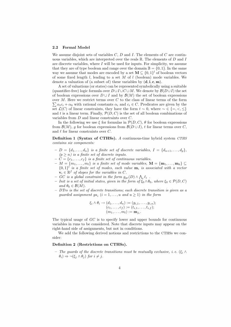
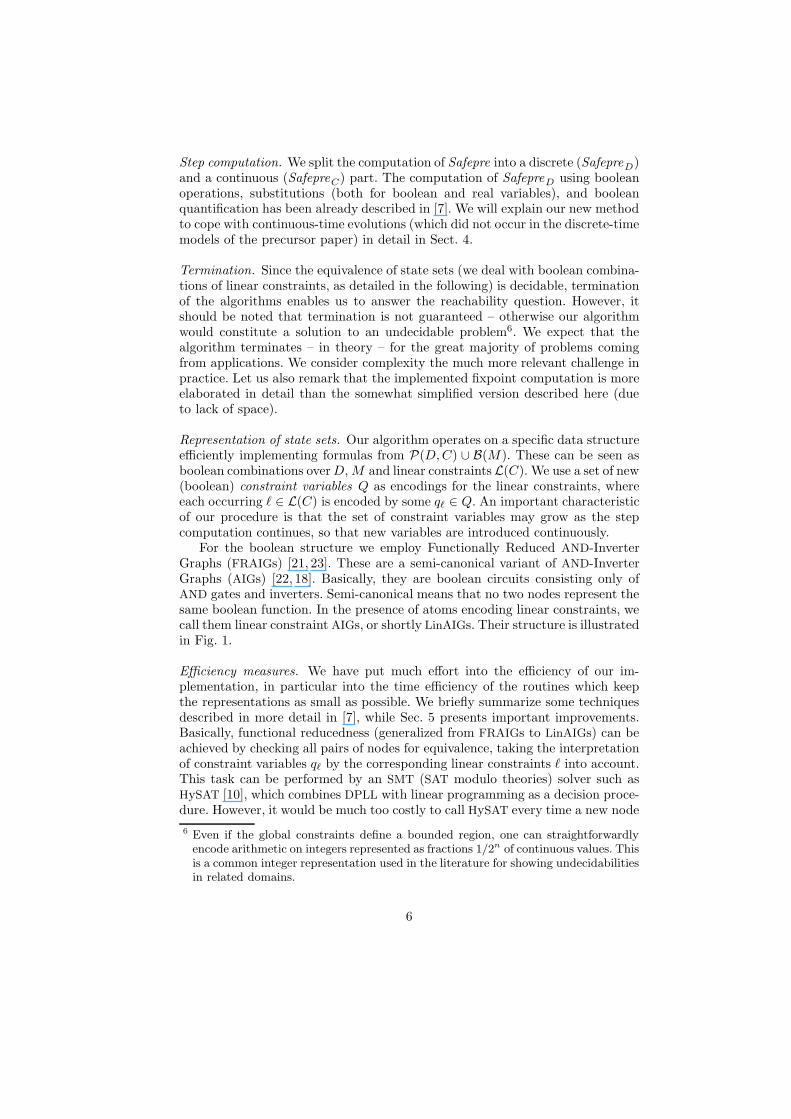
For the boolean structure we employ Functionally Reduced AND-InverterGraphs (FRAIGs) [21, 23]. These are a semi-canonical variant of AND-InverterGraphs (AIGs) [22, 18]. Basically, they are boolean circuits consisting only ofAND gates and inverters. Semi-canonical means that no two nodes represent thesame boolean function. In the presence of atoms encoding linear constraints, wecall them linear constraint AIGs, or shortly LinAIGs. Their structure is illustratedin Fig. 1.

Efficiency measures. We have put much effort into the efficiency of our im-plementation, in particular into the time efficiency of the routines which keepthe representations as small as possible. We briefly summarize some techniquesdescribed in more detail in [7], while Sec. 5 presents important improvements.Basically, functional reducedness (generalized from FRAIGs to LinAIGs) can beachieved by checking all pairs of nodes for equivalence, taking the interpretationof constraint variables qℓ by the corresponding linear constraints ℓ into account.This task can be performed by an SMT (SAT modulo theories) solver such asHySAT [10], which combines DPLL with linear programming as a decision proce-dure. However, it would be much too costly to call HySAT every time a new node

6 Even if the global constraints define a bounded region, one can straightforwardlyencode arithmetic on integers represented as fractions 1/2n of continuous values. Thisis a common integer representation used in the literature for showing undecidabilitiesin related domains.

6

...

...

...

...

ql1 qlj

mapping betweenlinear constraintsand bool. variables

AIG

f1 fi Represented first order predicates

d1 dn

lin. constraints

cfc1continuous domain variables

boolean domain variables

Fig. 1. The LinAIG structure

is introduced. Instead, a hierarchy of approximate techniques is used to factorout “easy” problem instances. In first steps purely boolean approximations areemployed: If two nodes represent equivalent boolean formulas, we do not need torefer to the definition of the constraint variables. Here we make use of capabilitiesof FRAIGs, which include local boolean normalization rules, simulation, and SAT

checks. Additionally, boolean reasoning is supported by (approximate) knowl-edge on linear constraints such as implications between constraints. For identi-fying non-equivalent LinAIG nodes we use test vectors with valuations c ∈ Rf ,and it proved to be worthwhile to use not only randomly generated test vectors,but also test vectors extracted from failed exact checks done by HySAT (learningtest vectors). All of these techniques are arranged in a carefully designed andtested strategy of when to apply which technique.

4 Flow extrapolation

Continuous transitions. In our system model, the time steps only concern theevolutions of continuous variables and leave the discrete part unchanged. Foreach mode, the continuous safe pre-image SafepreC can be expressed as a formulawith one quantified real variable (time). We will show how to eliminate thisquantifier to arrive at a formula which can again be represented by a LinAIG.

Let φ(D,M,Q) be a representation of a state set. Each valuation mi of themode variables in M encodes a concrete mode with an associated evolution vi

of C and boundary condition βi. Let φi be the cofactor of φ w. r. t. mode mi.

Thus we have φ ⇔∨k

i=1 φi ∧ (m1, . . . ,ml) = mi, where each φi is a booleanformula over D and Q. For each mode mi, we must now determine the set of allvaluations for which every (arbitrarily long) evolution along vi remains in the setof valuations satisfying φi, either forever or until it meets a point that satisfiesthe boundary condition βi or violates the global constraints GC . We denote thisset by SafepreC(φi,vi, βi). Logically, it can be described by the formula

∀λ.(

λ < 0 ∨ φi(c+λvi) ∨ ¬GC (c+λvi)∨ ∃λ′. (λ′ ≥ 0 ∧ λ′ < λ ∧ (βi(c+λ

′vi) ∨ ¬GC (c+λ′vi))))

.

Under the assumption that the set described by GC is convex, and usingthe fact that we are only interested in states satisfying GC , this formula can be

7

simplified (modulo GC ) to

∀λ.(

λ < 0 ∨ φi(c+λvi) ∨ ¬GC (c+λvi) ∨ ∃λ′. (λ′ ≥ 0 ∧ λ′ < λ ∧ βi(c+λ′vi))

)

.

Our task is now to convert this formula over λ, λ′, C, andD into an equivalentformula over the original variables in C and D. If the variables in C occur in φand β only within linear constraints, then this amounts to variable eliminationfor linear real arithmetic.7

Test points. The Loos-Weispfenning test point method [19, 9] eliminates univer-sal quantifiers by converting them into finite conjunctions (and dually, existen-tial quantifiers into finite disjunctions). The method is based on the followingobservation: Assume that a formula ψ(x, ~y) is written as a positive booleancombination of linear constraints x ∼i ti(~y) and 0 ∼′

j t′j(~y), where ∼i,∼′j ∈

{=, 6=, <,≤, >,≥}. Let us keep the values of ~y fixed for a moment. If the set ofall x such that ψ(x, ~y) does not hold is non-empty, then it can be written as afinite union of (possibly unbounded) intervals, whose boundaries are among theti(~y). To check whether ∀x. ψ(x, ~y) holds, it is therefore sufficient to test ψ(x, ~y)for either all upper or all lower boundaries of these intervals. The test values mayinclude +∞, −∞, or a positive infinitesimal ε, but these can easily be eliminatedfrom the substituted formula. For instance, if x is substituted by tj(~y)− ε, thenboth the linear constraints x ≤ ti(~y) and x < ti(~y) are turned into tj(~y) ≤ ti(~y),and both x ≥ ti(~y) and x > ti(~y) are turned into tj(~y) > ti(~y).

There are two possible sets of test points, depending on whether we considerupper or lower boundaries:

TP1 = {+∞}∪ { ti(~y) | ∼i ∈ {6=, >} } ∪ { ti(~y) − ε | ∼i ∈ {=,≥} }

TP2 = {−∞} ∪ { ti(~y) | ∼i ∈ {6=, <} } ∪ { ti(~y) + ε | ∼i ∈ {=,≤} }.

Let TP be the smaller one of the two sets and let T be the set of all symbolicsubstitutions x/t for t ∈ TP . Then the formula ∀x. ψ(x, ~y) can be replaced by anequivalent finite conjunction

∧

σ∈T ψ(x, ~y)σ. The size of TP is in general linear inthe size of ψ, so the size of the resulting formula is quadratic in the size of ψ. Thisis independent of the boolean structure of ψ – conversion to CNF is not required.On the other hand, if ψ is a conjunction

∧

ψi, then the test point method can alsobe applied to each of the formulas ψi individually, leading to a smaller numberof test points. Moreover, when the test point method transforms each ψi into afinite conjunction

∧

ψji , then each ψj

i contains at most as many linear constraintsas the original ψi, and only the length of the outer conjunction increases.

Applying the test point method to flow extrapolation. We have demonstratedabove that the safe pre-image SafepreC(φi,vi, βi) of the formula φi is

∀λ.(

λ < 0 ∨ φi(c+λvi) ∨ ¬GC (c+λvi) ∨ ∃λ′. (λ′ ≥ 0 ∧ λ′ < λ ∧ βi(c+λ′vi))

)

.

7 The variables in D are assumed to remain constant during mode mi, so booleanexpressions over D behave like propositional variables. For simplicity, we will ignorethem in the rest of this section.

8

Assuming that φi equals∧

k φik and that βi equals∨

j βij , we obtain

∧

k ∀λ.(

λ < 0 ∨ φ′ik(c+λvi) ∨∨

j ∃λ′. (λ′ ≥ 0 ∧ λ′ < λ ∧ βij(c+λ

′vi)))

.

where φ′ik abbreviates φik ∨ ¬GC . Applying the test point method, we replacethe universal and the existential quantifier by a finite conjunction or disjunctionusing a set of symbolic substitutions T ′

j for λ′ (which depends on βij and vi) anda set of symbolic substitutions Tk for λ (which depends on φik, the βij , and vi):

SafepreC(φi,vi, βi) =∧

k

∧

σ∈Tk

(

(λ < 0 ∨ φ′ik(c + λvi))σ

∨∨

j

∨

τ∈T ′

j(λ′ ≥ 0 ∧ λ′ < λ ∧ βij(c + λ′vi))τσ

)

.

Note that the test point method can work directly on the internal formularepresentation of LinAIGs – in contrast to the classic Fourier-Motzkin algorithm,there is no need for a costly CNF or DNF conversion before eliminating quanti-fiers. Moreover, the resulting formulas preserve most of the boolean structure ofthe original ones: the method behaves largely like a generalized substitution.

Convexity. It should be noted that some of the complexity of the general casedisappears automatically if the complement of the boundary conditions is con-vex, that is, if every βij is a single linear inequation. Consider the formula∨

τ∈T ′

j(λ′ ≥ 0∧ λ′ < λ∧ βij(c + λ′vi))τ . If βij is a single linear inequation, then

two test points are always sufficient:8 (a) If βij(c + λ′vi) has the form λ′ ≤ t(c)or λ′ < t(c), then the test points are −∞ and 0, (b) otherwise, if βij(c + λ′vi)has the form λ′ ≥ t(c) or λ′ > t(c), or if λ′ is cancelled out completely inβij(c+λ′vi), then the test points are +∞ and λ− ε. Moreover, if +∞ or −∞ issubstituted for λ′, the conjunction becomes trivially false, so the whole formulais reduced to 0 < λ∧βij(c) in case (a) and to λ > 0∧βij(c+(λ−ε)vi) in case (b).

5 Redundancy Elimination

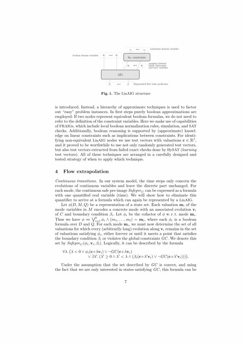
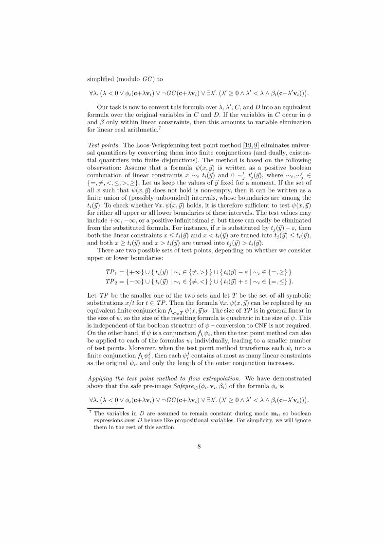
Our earlier experiments demonstrated that LinAIGs form an efficient data struc-ture for boolean combinations of boolean variables and linear constraints overreal variables [7]. However, in connection with flow extrapolation using Loos-Weispfennig quantifier elimination, one observes that the number of “redun-dant” linear constraints grows rapidly during the fixpoint iteration of the modelchecker. For illustration see Fig. 2 and 3, which show a typical example from amodel checking run representing a small state set based on two real variables:Lines in Figures 2 and 3 represent linear constraints, and the gray shaded arearepresents the space defined by some boolean combination of these constraints.Whereas the representation depicted in Fig. 2 contains 24 linear constraints, acloser analysis shows that an optimized representation can be found using only15 linear constraints as depicted in Fig. 3.

8 Since we want to eliminate an existential quantifier, we have to use the dual form ofthe method described above.

9

Fig. 2. Before redundancy removal Fig. 3. After redundancy removal

Removing redundant constraints from our representations turned out to bea crucial task for the success of our methods. It should be noted that, sincewe represent arbitrary boolean combinations of linear constraints (and booleanvariables), this task is not as straightforward as for other approaches such as [14,11] which represent sets of convex polyhedra, i. e., sets of conjunctions ℓ1 ∧ . . .∧ℓn of linear constraints. If one is restricted to convex polyhedra, the questionwhether a linear constraint ℓ1 is redundant in the representation reduces to thequestion whether ℓ2 ∧ . . .∧ ℓn represents the same polyhedron as ℓ1 ∧ . . .∧ ℓn, orequivalently, whether ℓ1 ∧ ℓ2 ∧ . . . ∧ ℓn represents the empty set. This questioncan simply be answered by a linear constraint solver.

For redundancy elimination in our context consider a predicate F (b1, . . . , bk,ℓ1, . . . , ℓn) (represented by a LinAIG) where b1, . . . , bk are boolean variables,ℓ1, . . . , ℓn are linear constraints over C, and F is a boolean function.

Definition 4 (Redundancy of linear constraints). The linear constraintsℓ1, . . . , ℓr (1 ≤ r ≤ n) are called redundant in the representation of F (b1, . . . , bk,ℓ1, . . . , ℓn) iff there is a boolean function G with the property that F (b1, . . . , bk, ℓ1,. . . , ℓn) and G(b1, . . . , bk, ℓr+1, . . . , ℓn) represent the same predicates.

In order to be able to check for redundancy, we need a disjoint copy C′ ={c′1, . . . , c

′f} of the continuous variables C = {c1, . . . , cf}. Moreover, for each

linear constraint ℓi (1 ≤ i ≤ n) we introduce a corresponding linear constraintℓ′i which coincides with ℓi up to replacement of variables cj ∈ C by variablesc′j ∈ C′. Our check for redundancy is based on the following theorem:

Theorem 5 (Redundancy check). The linear constraints ℓ1, . . . , ℓr (1 ≤ r ≤n) are redundant in the representation of F (b1, . . . , bk, ℓ1, . . . , ℓn) iff the predicate

F (b1, . . . , bk, ℓ1, . . . , ℓn) ⊕ F (b1, . . . , bk, ℓ′1, . . . , ℓ

′n) ∧

∧n

i=r+1(ℓi ≡ ℓ′i) (1)

(where ⊕ denotes exclusive-or) is not satisfiable by any assignment of booleanvalues to b1, . . . , bk and real values to the variables c1, . . . , cf , c′1, . . . , c

′f .

Note that the check from Thm. 5 can be performed by an SMT solver suchas HySAT [10]. For completeness a proof of Thm. 5 is given in Appendix A. Herewe just give a sketch of the intuition behind Thm. 5.

According to Def. 4 linear constraints ℓ1, . . . , ℓn are redundant iff there is aboolean function G such that G(b1, . . . , bk, ℓr+1, . . . , ℓn) and F (b1, . . . , bk, ℓ1, . . . ,

10

ℓn) represent the same predicates. Now let us look at F (b1, . . . , bk, ℓ1, . . . , ℓn)as a boolean function F (b1, . . . , bk, qℓ1 , . . . , qℓn

) with (new) boolean constraintvariables qℓ1 , . . . , qℓn

and a mapping connecting qℓito ℓi (just as in our definition

of LinAIGs). In comparison to F the required boolean function G must dependonly on variables b1, . . . , bk, qℓr+1

, . . . , qℓn.

If formula (1) is satisfied by some assignment d ∈ {0, 1}k to the booleanvariables b1, . . . , bk, c ∈ Rf to the real variables c1, . . . , cf (which are inputs oflinear constraints ℓi), and c′ ∈ Rf to the copied real variables c′1, . . . , c

′f (which

are inputs of copied linear constraints ℓ′i), then the first part of formula (1),i. e. F (b1, . . . , bk, ℓ1, . . . , ℓn)⊕F (b1, . . . , bk, ℓ

′1, . . . , ℓ

′n) enforces that the predicate

F changes its value if input c is replaced by input c′ in the corresponding linearconstraints. On the other hand, the second part

∧n

i=r+1(ℓi ≡ ℓ′i) enforces that thetruth assignment to linear constraints ℓr+1, . . . , ℓn does not change when replac-ing c by c′. However, since G only depends on variables b1, . . . , bk, qℓr+1

, . . . , qℓn

(whose truth assignments are not changed), function G “cannot see” the effectof changing c to c′. Thus G is not able to change its value like F when replacingc by c′ and therefore it is not able to represent the same predicate as F .

Conversely, it can be seen that an appropriate function G can be constructed,when formula (1) is unsatisfiable. When constructing G, we use the notion of thedon’t care set DC induced by linear constraints ℓ1, . . . , ℓn: This don’t care setDC := {(vb1 , . . . vbk

, vℓ1 , . . . , vℓn) | ∄(vc1

, . . . vcf) ∈ Rf with ℓi(vc1

, . . . , vcf) =

vℓi∀1 ≤ i ≤ n} contains all boolean combinations which can not occur due to

inconsistent assignments to boolean constraint variables. Whereas for all (d, c) ∈DC := {0, 1}k+n \DC we have to postulate G(d, c) = F (d, c), the value of Gmay be chosen arbitrarily for all (d, c) ∈ DC, since these values can not occurdue to inconsistencies between linear constraints. A closer analysis shows that– under assumption of unsatisfiability of formula (1) – it is indeed possible todefine the function values of G(d, c) for (d, c) ∈ DC in such a way that G willnot depend on variables qℓ1 , . . . , qℓr

. This proves that linear constraints ℓ1, . . . , ℓrare then redundant. (For details see Appendix A.)

A straightforward realization of this approach would need a (compact) repre-sentation of the don’t care set DC in order to compute an appropriate booleanfunction G. However, two interesting observations turn the basic idea into afeasible approach:

1. In general, we do not need the complete set DC for the definition of theboolean function G.

2. A representation of a subset of DC which is needed for removing the re-dundant constraints ℓ1, . . . , ℓr is already computed by an SMT solver whenchecking satisfiability of formula (1).

Details on how the SMT solver internally computes a representation of a sufficientsubset of DC and on the actual removal of redundant constraints are includedin Appendix B. Our ideas for redundancy detection and removal have beenimplemented based on the SMT solver HySAT. Experiments given in Section6 show that integrating redundancy removal is crucial for the success of ourmethods.

11

6 Experimental Results

Our sample application is derived from a case study for Airbus, a controller forthe flaps of an aircraft [13]. The flaps are extended during take-off and land-ing to generate more lift at low velocity. They are not robust enough for highvelocity, so they must be retracted for other periods. It is the controller’s taskto correct the pilot’s commands if he endangers the flaps. Additionally, thereis also an extensive monitoring of the health of its sub-systems, checking forinstance for hardware failures. The health monitoring system interacts with theflap control by enforcing a more conservative behavior of the control when errorsare supposed to be in the system.

The benchmark used here is a simplified version of the full system includingthe flap controller and a health monitoring system, which is triggered by a timer.The model has three continuous variables: the velocity, the flap angle, and thetimer value. Discrete states of the controller and of the health monitoring systemcontribute to the discrete state space. The discrete state space contains 220

discrete states. This size is clearly out of reach for hybrid verification tools knownfrom the literature, which do not scale in the discrete dimension, since modes –the only discrete states considered – are represented explicitly when performingreachability analysis.

The safety property to be established for our model is “For the current flapsetting, the aircraft’s velocity shall not exceed the nominal velocity (w. r. t. theflap position) plus 7 knots”. Whether this requirement holds for our model de-pends on a “race” between flap retraction and speed increase. The controller iscorrect, if it initiates flap retraction (by correcting the pilot) early enough.

Based on the ideas presented in the previous sections we implemented aprototype model checker using LinAIGs for representing sets of states. Our ex-periments were run on an AMD Opteron with 2.6 GHz and 16 GB RAM.

Our model checker was able to prove the given safety invariant for the casestudy in 888.6 CPU seconds. The LinAIG representation had a maximum numberof 30887 nodes and a maximum number of 80 linear constraints. The numberof flow extrapolation steps using Loos-Weispfennig quantifier elimination was 6,the number of discrete image computation steps performed until reaching thefixpoint was 20. This result clearly demonstrates that our approach is able tosuccessfully verify hybrid systems including discrete parts with state spaces ofconsiderable sizes.

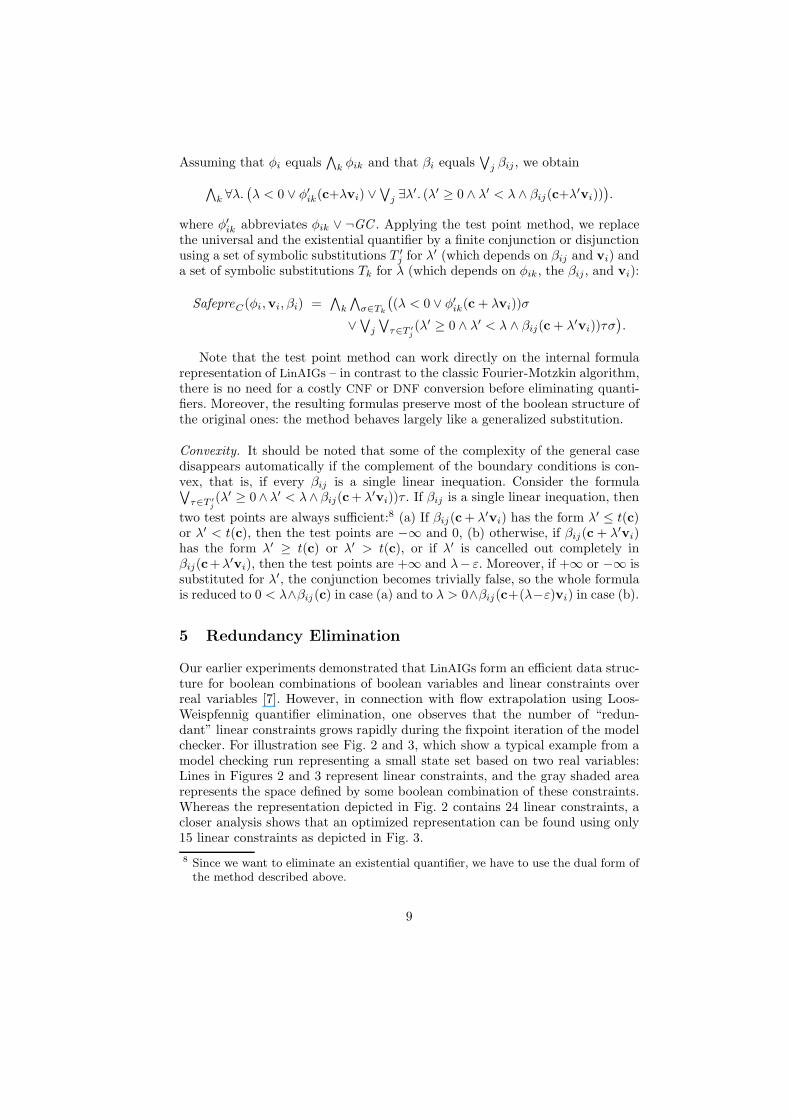
In the following we analyze how the individual ingredients of our methodcontribute to its overall success. Redundancy elimination turned out to be ab-solutely necessary to make flow extrapolation using Loos-Weispfennig quantifierelimination feasible. Fig. 4 illustrates the difference between the model check-ing runs for our case study with and without redundancy removal by plottingthe numbers of linear constraints used during the model checking run. Withoutredundancy removal (dotted line), the number of linear constraints is rapidlyincreasing up to a number of 1000 linear constraints and 150000 LinAIG nodesin the fourth flow extrapolation.9 On the other hand, redundancy elimination

9 Without redundancy removal the remaining two flow extrapolations could not beperformed within our timeout of 24 hours.

12

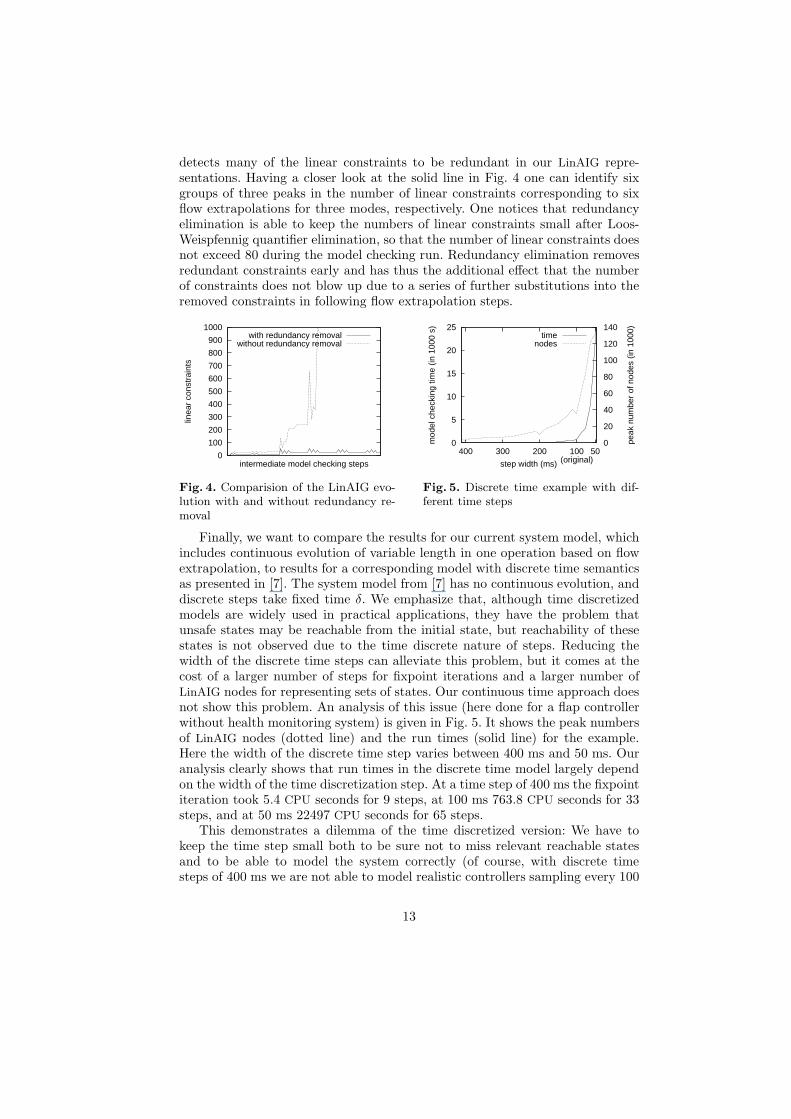
detects many of the linear constraints to be redundant in our LinAIG repre-sentations. Having a closer look at the solid line in Fig. 4 one can identify sixgroups of three peaks in the number of linear constraints corresponding to sixflow extrapolations for three modes, respectively. One notices that redundancyelimination is able to keep the numbers of linear constraints small after Loos-Weispfennig quantifier elimination, so that the number of linear constraints doesnot exceed 80 during the model checking run. Redundancy elimination removesredundant constraints early and has thus the additional effect that the numberof constraints does not blow up due to a series of further substitutions into theremoved constraints in following flow extrapolation steps.

0

100

200

300

400

500

600

700

800

900

1000

linea

r co

nstr

aint

s

intermediate model checking steps

with redundancy removalwithout redundancy removal

Fig. 4. Comparision of the LinAIG evo-lution with and without redundancy re-moval

0

5

10

15

20

25

400 300 200 100(original)

50 0

20

40

60

80

100

120

140

mod

el c

heck

ing

time

(in 1

000

s)

peak

num

ber

of n

odes

(in

100

0)

step width (ms)

timenodes

Fig. 5. Discrete time example with dif-ferent time steps

Finally, we want to compare the results for our current system model, whichincludes continuous evolution of variable length in one operation based on flowextrapolation, to results for a corresponding model with discrete time semanticsas presented in [7]. The system model from [7] has no continuous evolution, anddiscrete steps take fixed time δ. We emphasize that, although time discretizedmodels are widely used in practical applications, they have the problem thatunsafe states may be reachable from the initial state, but reachability of thesestates is not observed due to the time discrete nature of steps. Reducing thewidth of the discrete time steps can alleviate this problem, but it comes at thecost of a larger number of steps for fixpoint iterations and a larger number ofLinAIG nodes for representing sets of states. Our continuous time approach doesnot show this problem. An analysis of this issue (here done for a flap controllerwithout health monitoring system) is given in Fig. 5. It shows the peak numbersof LinAIG nodes (dotted line) and the run times (solid line) for the example.Here the width of the discrete time step varies between 400 ms and 50 ms. Ouranalysis clearly shows that run times in the discrete time model largely dependon the width of the time discretization step. At a time step of 400 ms the fixpointiteration took 5.4 CPU seconds for 9 steps, at 100 ms 763.8 CPU seconds for 33steps, and at 50 ms 22497 CPU seconds for 65 steps.

This demonstrates a dilemma of the time discretized version: We have tokeep the time step small both to be sure not to miss relevant reachable statesand to be able to model the system correctly (of course, with discrete timesteps of 400 ms we are not able to model realistic controllers sampling every 100

13

ms). However, decreasing the time step too much may turn the model checkingproblem intractable. In contrast, in our novel approach we do not work with timediscretizations, but we are able to compute continuous evolutions of variablelengths in one operation based on flow extrapolation. Sequences of discrete stepsof the previous version [7] where no mode switches are triggered are collapsedinto a single symbolic substitution in this way. Note that in the example withouthealth monitoring system only five flow extrapolation steps are needed to reachthe fixpoint within a runtime of 27.7 s (whereas for the discrete time model witha time step of 50 ms, e. g., the number of steps amounts to 65 with a run timeof 22497 s).

7 Conclusion

We consider the tight integration of LinAIGs and HySAT in backward reachabil-ity analysis a core technology to address scalability of hybrid system verificationmethods with large discrete state spaces, and have demonstrated the relevanceof the approach using a benchmark derived from an Airbus flap controller. Theredundancy elimination technique presented in Section 5 is of independent valueand could be integrated in other hybrid verification tools. Next imminent exten-sions of our approach cover differential inclusions and continuous inputs. We willexperiment with incorporating orthogonal extensions to our approach such as ex-ploiting robustness, over-approximation, and counterexample guided abstractionrefinement to address richer dynamics and achieve further scalability.

References

1. M. Agrawal and P. S. Thiagarajan. Lazy rectangular hybrid automata. In 7th

Workshop on Hybrid Systems: Computation and Control, 2004, LNCS 2993, pp.1–15. Springer.

2. M. Agrawal and P. S. Thiagarajan. The discrete time behavior of lazy linear hybridautomata. In 8th Workshop on Hybrid Systems: Computation and Control, 2005,LNCS 3414, pp. 55–69. Springer.

3. R. Alur, C. Courcoubetis, N. Halbwachs, T. A. Henzinger, P.-H. Ho, X. Nicollin,A. Olivero, J. Sifakis, and S. Yovine. The algorithmic analysis of hybrid systems.Theoretical Computer Science, 138(1):3–34, 1995.

4. E. Asarin, T. Dang, and A. Girard. Hybridization methods for the analysis ofnon-linear systems. Acta Informatica, 43(7):451–476, 2007.

5. E. Asarin, T. Dang, and O. Maler. The d/dt tool for verification of the hybridsystems. In 14th Conference on Computer Aided Verification, 2002, LNCS 2404,pp. 365–370. Springer.

6. B. Boigelot and F. Herbreteau. The power of hybrid acceleration. In 18th Confer-

ence on Computer Aided Verification, 2006, LNCS 4144, pp. 438–451. Springer.7. W. Damm, S. Disch, H. Hungar, J. Pang, F. Pigorsch, C. Scholl, U. Waldmann,

and B. Wirtz. Automatic verification of hybrid systems with large discrete statespace. In 4th Symposium on Automated Technology for Verification and Analysis,2006, LNCS 4218, pp. 276–291.

8. W. Damm, G. Pinto, and S. Ratschan. Guaranteed termination in the verificationof LTL properties of non-linear robust discrete time hybrid systems. Journal of

Foundations of Computer Science, 18(1):63–86, 2007.

14

9. A. Dolzmann. Algorithmic Strategies for Applicable Real Qunantifier Elimination.PhD thesis, Universitat Passau, 2000.

10. M. Franzle and C. Herde. HySAT: An efficient proof engine for bounded modelchecking of hybrid systems. Formal Methods in System Design, 30(3):179–198,2007.

11. G. Frehse. Compositional Verification of Hybrid Systems using Simulation Rela-

tions. PhD thesis, Radboud Universiteit Nijmegen, 2005.12. A. Girard and G. J. Pappas. Approximation metrics for discrete and continuous

systems. IEEE Transactions on Automatic Control, 52(5):782–798, 2007.13. H3 FOMC Team. The flap controller description. http://www.avacs.org/

Benchmarks/Open/flapcontroller.pdf.14. T. A. Henzinger. The theory of hybrid automata. In 11th IEEE Symposium on

Logic in Computer Science, 1996, pp. 278–292. IEEE Press.15. T. A. Henzinger, P.-H. Ho, and H. Wong-Toi. HyTech: A model checker for hybrid

systems. Software Tools for Technology Transfer, 1(1–2):110–122, 1997.16. C. A. R. Hoare. An axiomatic basis for computer programming. Communication

of the ACM, 12:576–583, 1969.17. S. Jha, B. Brady, and S. Seshia. Symbolic reachability analysis of lazy linear hybrid

automata. Technical report, EECS Dept., UC Berkeley, 2007.18. A. Kuehlmann, V. Paruthi, F. Krohm, and M. K. Ganai. Robust boolean reasoning

for equivalence checking and functional property verification. IEEE Transactions

on Computer-Aided Design, 21(12):1377–1394, 2002.19. R. Loos and V. Weispfenning. Applying linear quantifier elimination. The Com-

puter Journal, 36(5):450–462, 1993.20. K. L. McMillan. Symbolic Model Checking. Kluwer Academic Publishers, 1993.21. A. Mishchenko, S. Chatterjee, R. Jiang, and R. K. Brayton. FRAIGs: A unifying

representation for logic synthesis and verification. Technical report, EECS Dept.,UC Berkeley, 2005.

22. V. Paruthi and A. Kuehlmann. Equivalence checking combining a structural SAT-solver, BDDs, and simulation. In 18th IEEE Conference on Computer Design,2000, pp. 459–464. IEEE Press.

23. F. Pigorsch, C. Scholl, and S. Disch. Advanced unbounded model checking byusing AIGs, BDD sweeping and quantifier scheduling. In 6th Conference on Formal

Methods in Computer Aided Design, 2006, pp. 89–96. IEEE Press.24. A. Platzer and E. Clarke. The image computation problem in hybrid systems

model checking. In 10th Workshop on Hybrid Systems: Computation and Control,2007, LNCS 4416, pp. 473–486. Springer.

25. M. Segelken. Abstraction and counterexample-guided construction of ω-automatafor model checking of step-discrete linear hybrid models. In 19th Conference on

Computer Aided Verification, 2007, LNCS. Springer. To appear.26. B. I. Silva, K. Richeson, B. H. Krogh, and A. Chutinan. Modeling and verification

of hybrid dynamical system using CheckMate. In 4th Conference on Automation

of Mixed Processes, 2000.27. The VIS Group. VIS: A system for verification and synthesis. In 8th Conference

on Computer Aided Verification, 1996, LNCS 1102, pp. 428–432. Springer.28. F. Wang. Symbolic parametric safety analysis of linear hybrid systems with BDD-

like data-structures. IEEE Transactions on Software Engineering, 31(1):38–52,2005.

15

A Appendix: Proof of Theorem 5

“if-part”: For the proof of the “if-part” of Theorem 5 (see page 10) we assumethat the predicate from formula (1) is satisfiable and under this assumptionwe prove that it can not be the case that all linear constraints ℓ1, . . . , ℓr areredundant.

Now consider some satisfying assignment to the predicate from formula (1) asfollows: b1 = vb1 , . . . , bk = vbk

with (vb1 , . . . vbk) ∈ {0, 1}k, c1 = vc1

, . . . , cf = vcf

with (vc1, . . . vcf

) ∈ Rf , c′1 = vc′1, . . . , c′f = vc′

fwith (vc′

1, . . . vc′

f) ∈ Rf . This sat-

isfying assignment implies a corresponding truth assignment to the linear con-straints by ℓi(vc1

, . . . vcf) = vℓi

(1 ≤ i ≤ n) with vℓi∈ {0, 1} and ℓ′i(vc′

1, . . . vc′

f) =

vℓ′i

(1 ≤ i ≤ n) with vℓ′i∈ {0, 1}. Since the assignment satisfies formula (1), it

holds that

F (vb1 , . . . , vbk, vℓ1 , . . . , vℓn

) 6= F (vb1 , . . . , vbk, vℓ′

1, . . . , vℓ′n

), (a)vℓi

= vℓ′i

for all r + 1 ≤ i ≤ n. (b)

If the linear constraints ℓ1, . . . , ℓr (1 ≤ r ≤ n) would be redundant in the rep-resentation of F (b1, . . . , bk, ℓ1, . . . , ℓn), then there had to be a boolean functionG with G(b1, . . . , bk, ℓr+1, . . . , ℓn) and F (b1, . . . , bk, ℓ1, . . . , ℓn) representing thesame predicates, and thus

G(vb1 , . . . , vbk, vℓr+1

, . . . , vℓn) = F (vb1 , . . . , vbk

, vℓ1 , . . . , vℓn), (c)

G(vb1 , . . . , vbk, vℓ′

r+1, . . . , vℓ′n

) = F (vb1 , . . . , vbk, vℓ′

1, . . . , vℓ′n

). (d)

Altogether we have

G(vb1 , . . . vbk, vℓr+1

, . . . , vℓn)

(c)= F (vb1 , . . . , vbk

, vℓ1 , . . . , vℓr, vℓr+1

, . . . , vℓn)

(a)

6= F (vb1 , . . . , vbk, vℓ′

1, . . . , vℓ′r

, vℓ′r+1

, . . . , vℓ′n)

(d)= G(vb1 , . . . , vbk

, vℓ′r+1, . . . , vℓ′n

)(b)= G(vb1 , . . . , vbk

, vℓr+1, . . . , vℓn

)

which is a contradiction. Thus, it is not true that all linear constraints ℓ1, . . . , ℓrare redundant. 2

“then-part”: Here we assume that there is no satisfying assignment to formula(1) and we show how to construct a boolean function G with G(b1, . . . , bk, ℓr+1,. . . , ℓn) and F (b1, . . . , bk, ℓ1, . . . , ℓn) representing the same predicates. To do so,we look at F (b1, . . . , bk, ℓ1, . . . , ℓn) as a boolean function F (b1, . . . , bk, qℓ1 , . . . , qℓn

)with (new) boolean constraint variables qℓ1 , . . . , qℓn

and a mapping connectingqℓi

to ℓi (just as in our definition of LinAIGs). In comparison to F the requiredboolean function G depends only on variables b1, . . . , bk, qℓr+1

, . . . , qℓn. For defin-

ing G we will need the notion of the don’t care set DC induced by linear con-straints ℓ1, . . . , ℓn: This don’t care set

DC := {(vb1 , . . . vbk, vℓ1 , . . . , vℓn

) | ∄(vc1, . . . vcf

) ∈ Rf

with ℓi(vc1, . . . , vcf

) = vℓi∀1 ≤ i ≤ n}

16

contains all boolean combinations which can not occur due to inconsistent as-signments to boolean constraint variables.

Whereas for all (vb1 , . . . vbk, vℓ1 , . . . , vℓn

) ∈ DC := {0, 1}k+n \ DC we haveto postulate G(vb1 , . . . vbk

, vℓr+1, . . . , vℓn

) = F (vb1 , . . . vbk, vℓ1 , . . . , vℓn

) in orderto achieve that G(b1, . . . , bk, ℓr+1, . . . , ℓn) and F (b1, . . . , bk, ℓ1, . . . , ℓn) representthe same predicates, the value of G may be chosen arbitrarily for all ǫ ∈ DC,since these values can not occur due to inconsistencies between linear constraints.Now the idea is to define the function values of G(ǫ) for ǫ ∈ DC in such a waythat G will not depend on variables qℓ1 , . . . , qℓr

.For the definition of G we additionally consider for arbitrary values (vb1 , . . . ,

vbk, vℓr+1

, . . . , vℓn) ∈ {0, 1}k+n−r the sets

orbit(vb1 , . . . , vbk, vℓr+1

, . . . , vℓn) :=

{(vb1 , . . . , vbk, vℓ1 , . . . , vℓr

, vℓr+1, . . . , vℓn

) | (vℓ1 , . . . , vℓr) ∈ {0, 1}r}.

For each (vb1 , . . . vbk, vℓr+1

, . . . , vℓn) ∈ {0, 1}k+n−r we define

– If orbit(vb1 , . . . vbk, vℓr+1

, . . . , vℓn)\DC 6= ∅, G(vb1 , . . . vbk

, vℓr+1, . . . , vℓn

) = δwith F (orbit(vb1 , . . . vbk

, vℓr+1, . . . , vℓn

) \DC) = {δ}, δ ∈ {0, 1}.– Otherwise G(vb1 , . . . vbk

, vℓr+1, . . . , vℓn

) is chosen arbitrarily.

It is clear that G does not depend on variables qℓ1 , . . . , qℓrby this definition.

However it remains to be shown that G is well-defined, i. e., that

|F (orbit(vb1 , . . . vbk, vℓr+1

, . . . , vℓn) \DC)| = 1.

Suppose that G is not well-defined, i. e., there is some set

orbit(vb1 , . . . vbk, vℓr+1

, . . . , vℓn) \DC

which contains two different elements

v(1) := (vb1 , . . . , vbk, vℓ1 , . . . , vℓr

, vℓr+1, . . . , vℓn

)

andv(2) := (vb1 , . . . , vbk

, v′ℓ1 , . . . , v′ℓr, vℓr+1

, . . . , vℓn)

with F (v(1)) 6= F (v(2)). Since v(1) /∈ DC, we know that there are (vc1, . . . , vcf

) ∈

Rf with ℓi(vc1, . . . vcf

) = vℓifor all 1 ≤ i ≤ n and since v(2) /∈ DC there are

(v′c1, . . . , v′cf

) ∈ Rf with ℓi(v′c1, . . . v′cf

) = v′ℓifor all 1 ≤ i ≤ r, ℓi(v

′c1, . . . v′cf

) =vℓi

for all r + 1 ≤ i ≤ n.It is easy to see that in this case b1 = vb1 , . . . , bk = vbk

, c1 = vc1, . . . , cf = vcf

,and c′1 = v′c1

, . . . , c′f = v′cfforms a satisfying assignment of formula (1) (with

ℓi(vc1, . . . vcf

) = vℓifor all 1 ≤ i ≤ r, ℓ′i(v

′c1, . . . v′cf

) = v′ℓifor all 1 ≤ i ≤ r,

ℓi(vc1, . . . vcf

) = ℓ′i(v′c1, . . . v′cf

) = vℓifor all r+ 1 ≤ i ≤ n.). This contradicts our

assumption that formula (1) is unsatisfiable, i. e., G is well-defined indeed. 2

B Appendix: Redundancy Removal Using an SMT Solver

In Section 5 we described a method for removing redundant linear constraintsfrom a predicate F (b1, . . . , bk, ℓ1, . . . , ℓn) resulting in a predicate G(b1, . . . , bk,

17

ℓr+1, . . . , ℓn). The basic approach relies on a don’t care set DC induced by linearconstraints ℓ1, . . . , ℓn which is given by

DC := {(vb1 , . . . vbk, vℓ1 , . . . , vℓn

) | ∄(vc1, . . . vcf

) ∈ Rf

with ℓi(vc1, . . . , vcf

) = vℓi∀1 ≤ i ≤ n}.

DC contains all boolean combinations which can not occur due to inconsis-tent assignments to boolean constraint variables.

Instead of computing the complete don’t care set DC we rather computerepresentations of subsets of DC which are needed for removing the redundantconstraints ℓ1, . . . , ℓr. Here we show how these sets can be computed by an SMT

solver during the check for satisfiability of formula (1) (see page 10).In order to explain how the appropriate subset of DC is computed by the

SMT solver we need to have a closer look at the function of an SMT solver likeHySAT [10]:

Just as in LinAIGs the SMT solver introduces constraint variables qℓifor

linear constraints ℓi. First, the SMT solver looks for satisfying assignments tothe boolean variables (including the constraint variables). Whenever the SMT

solver detects a satisfying assignment to the boolean variables, it checks whetherthe assignment to the constraint variables is consistent, i. e., whether it can beproduced by replacement of real variables by reals in linear constraints. Thistask is performed by a linear constraint solver. If the assignment is consistent,then the SMT solver has found a satisfying assignment, otherwise it continuessearching for satisfying assignments to the boolean variables. If some assignmentǫ1, . . . , ǫm to constraint variables qℓ1 , . . . , qℓm

was found to be inconsistent, then

the boolean “conflict clause” (qǫ1ℓ1

+ . . . + qǫm

ℓm) is added to the set of clauses in

the SMT solver to avoid running into the same conflict again. The negation ofthis conflict clause describes a set of don’t cares due to an inconsistency of linearconstraints.

Now consider formula (1) (see page 10) which has to be solved by an SMT

solver and suppose that the solver introduces boolean constraint variables qℓi

for linear constraints ℓi and qℓ′i

for ℓ′i (1 ≤ i ≤ n). According to Theorem 5,formula (1) is unsatisfiable when linear constraints ℓ1, . . . , ℓr are redundant. Thismeans that whenever there is some satisfying assignment to boolean variables(including constraint variables) in the SMT solver, it will be necessarily shownto be inconsistent. The most important observation is now that the negationsof conflict clauses due to these inconsistencies include the don’t cares needed tocompute a boolean function G which is appropriate in the sense of Definition 4:

If there is an orbit orbit(vb1 , . . . vbk, vℓr+1

, . . . , vℓn) containing two different el-

ements (vb1 , . . . , vbk, vℓ1 , . . . , vℓr

, vℓr+1, . . . , vℓn

) and (vb1 , . . . , vbk, v′ℓ1 , . . . , v

′ℓr,

vℓr+1, . . . , vℓn

) with F (vb1 , . . . vbk, vℓ1 , . . . , vℓr

, vℓr+1, . . . , vℓn

) 6= F (vb1 , . . . vbk, v′ℓ1 ,

. . . , v′ℓr, vℓr+1

, . . . , vℓn), then the following assignment to the boolean variables

obviously satisfies the boolean abstraction of formula (1) in the SMT solver:b1 = vb1 , . . . , bk = vbk

, qℓ1 = vℓ1 , . . . , qℓr= vℓr

, qℓ′1

= v′ℓ1 , . . . , qℓ′r = v′ℓr,

qℓr+1= qℓ′

r+1= vℓr+1

, . . . , qℓn= qℓ′n = vℓn

.

However, since we assumed that formula (1) is not satisfiable, this assignmentcan not be consistent wrt. the interpretation of constraint variables by linearconstraints. So there must be an inconsistency in the truth assignment to somelinear constraints ℓ1, . . . , ℓn, ℓ′1, . . . , ℓ

′n. Since the linear constraints ℓi and ℓ′j are

18

based on disjoint sets of real variables C = {c1, . . . , cf} and C′ = {c′1, . . . , c′f},

respectively, it is easy to see that a minimal number of assignments which arealready inconsistent performs only assignments to a subset of ℓ1, . . . , ℓn or a sub-set of ℓ′1, . . . , ℓ

′n. For this reason, when using the option of minimizing conflict

clauses, the SMT solver HySAT will learn a conflict clause whose negation ei-ther contains the don’t care (vb1 , . . . , vbk

, vℓ1 , . . . , vℓr, vℓr+1

, . . . , vℓn) or the don’t

care (vb1 , . . . , vbk, v′ℓ1 , . . . , v

′ℓr, vℓr+1

, . . . , vℓn). Since this consideration holds for

all pairs of elements in some orbit orbit(vb1 , . . . vbk, vℓr+1

, . . . , vℓn) for which F

produces different values, this means for the subset DC′ ⊆ DC of don’t caresdetected during the run of the SMT solver: |F (orbit(vb1 , . . . vbk

, vℓr+1, . . . , vℓn

) \DC′)| = 1, if orbit(vb1 , . . . vbk

, vℓr+1, . . . , vℓn

) \DC′ 6= ∅. Considering the defini-tion of G from Sect. 5 it is clear that the SMT solver HySAT thus computes alldon’t cares which are needed to generate the boolean function G not dependingon qℓ1 , . . . , qℓr

.A representation of the don’t cares needed may be extracted as a disjunc-

tion of negated conflict clauses which record inconsistencies between linear con-straints. In the end we obtain a boolean function dc from the SMT solver withON(dc) ⊆ DC10 and ON(dc) contains all needed don’t cares.

Finally, an appropriate function G is computed in the following way:

– At first by G′ = F · dc all don’t cares represented by dc are mapped to thefunction value 0.

– Secondly, we perform a existential quantification of the variables qℓ1 , . . . , qℓr

in G′: G = ∃qℓ1 , . . . , qℓrG′. This existential quantification maps all elements

of an orbit orbit(vb1 , . . . vbk, vℓr+1

, . . . , vℓn) to 1, whenever the orbit contains

an element ǫ with dc(ǫ) = 0 and F (ǫ) = 1. Since due to the argumentationabove there is no element δ in such an orbit with dc(δ) = 0 and F (δ) = 0,G eventually differs from F only for don’t cares defined by dc.

Altogether G does not depend on variables qℓ1 , . . . , qℓrand it is computed from

F only by changes of don’t cares defined by dc. This proves the correctness ofthe redundancy removal described above.

10 ON(dc) := {ǫ | dc(ǫ) = 1}

19