arX

iv:1

002.

2238

v2 [

hep-

th]

4 S

ep 2

010

Exact behavior of the energy density inside a one-dimensional oscillating cavitywith a thermal state

Danilo T. Alvesa, Edney R. Granhenb,c, Hector O. Silvaa,1,∗, Mateus G. Limac,d

aFaculdade de Fısica, Universidade Federal do Para, 66075-110, Belem, PA, BrazilbCentro Brasileiro de Pesquisas Fısicas, Rua Dr. Xavier Sigaud, 150, 22290-180, Rio de Janeiro, RJ, BrazilcFaculdade de Ciencias Exatas e Naturais, Universidade Federal do Para, 68505-080, Maraba, PA, Brazil

dFaculdade de Engenharia Eletrica, Universidade Federal do Para, 66075-110, Belem, PA, Brazil

Abstract

We investigate the exact behavior of the energy density of a real massless scalar field inside a cavity with a sin-gle moving mirror executing a resonant oscillatory law of motion, satisfying Dirichlet boundary conditions at finitetemperature. Our results are compared with those found in literature through analytical approximative methods.

Keywords: Dynamical Casimir effect, Energy density, Finite temperature, Oscillating cavityPACS:03.70.+k, 11.10.Wx, 42.50.Lc

1. Introduction

Since the pioneering work of Moore [1] and the subsequent works published in the 70s (for instance Refs. [2, 3, 4]),the problem of particle creation from vacuum due the interaction of a quantum field with moving mirrors (dynamicalCasimir effect) has been subject of intense theoretical study (for recent reviews see Refs. [5] and references therein).On the experimental side, the dynamical Casimir effect has not yet been observed, despite some experimental schemeshave been proposed based on simulation of a moving mirror by changing the reflectivity of a semiconductor usinglaser beams [6] or, more recently, using a coplanar waveguide terminated by a superconducting quantum interferencedevice [7].

In Ref. [1], Moore considered a real massless scalar field in atwo-dimensional spacetime inside a cavity withone moving boundary imposing Dirichlet boundary conditions on the field. He obtained the field solution in termsof the so-called Moore’s equation. Exact analytical solutions for particular laws of motion of the boundary [8], andalso approximative analytical solutions [9, 10] for the Moore’s equation were obtained but, so far, there is no generaltechnique to find analytical solutions for it. On the other hand, Cole and Schieve developed a geometrical approachto solve numerically and exactly Moore’s equation [11], obtaining the exact behavior of the energy density in a non-stationary cavity considering vacuum as the initial field state [11, 12]. The dynamical Casimir effect was also studiedwith different approaches from that adopted by Moore, via perturbative methods for a single mirror [13] and for anoscillating cavity [14].

The quantum problem of moving mirrors with initial field states different from vacuum was also analyzed [3,15, 16, 17, 18]. Specifically, a thermal bath was investigated for the case of a single mirror [15], and also for anoscillating cavity [16, 18]. In a recent paper [19], the present authors investigated the behavior of the energy densityinside a cavity with a moving mirror, for an arbitrary initial field state, obtaining formulas which enabled us to getexact numerical results for the quantum radiation force andfor the energy density in a non-static cavity for an arbitraryinitial field state and law of motion for the moving boundary.However, in Ref. [19] we applied our formulas only to

∗Corresponding authorEmail addresses:danilo@ufpa.br (Danilo T. Alves),edney@ufpa.br (Edney R. Granhen),hosilva@ufpa.br (Hector O. Silva ),

mateusl@ufpa.br (Mateus G. Lima)1Tel/Fax:+55 91 3201-7430 (Brazil)

Preprint submitted to Physics Letters A September 7, 2010

the case of an expanding cavity, with a non-oscillating movement and relativistic velocities. In the present letter, weconsider the exact approach developed in Ref. [19] to study the behavior of the energy density for a non-static cavitywith a thermal bath and a resonant oscillatory law of motion.We compare our results with those found by Andreataand Dodonov in Ref. [18] where this problem was investigatedthrough analytical approximative methods for smalloscillations. We show the limitations in the results obtained via this approach as the amplitude of oscillation growsto outside the small oscillations regime. We also investigate the energy density outside this regime for the first time.Additionally, we show that for small amplitudes of oscillation our results are in excellent agreement with [18].

This Letter is organized as follows: in Sec. 2 we obtain the field solution and the exact formulas for the energydensity taking the initial field state as a thermal bath and considering that the mirrors impose Dirichlet boundarycondition on the field. In Sec. 3 we study the behavior of the energy density for the case of an oscillatory law ofmotion for the moving boundary. Finally, in Sec. 4 we summarize our results.

2. Exact formulas for the energy density

Let us start considering the real massless scalar field satisfying the Klein-Gordon equation (we assume throughoutthis paper~ = c = kB = 1):

(∂2

t − ∂2x

)ψ (t, x) = 0, and obeying Dirichlet boundary conditions imposed at the static

boundary located atx = 0, and also at the moving boundary’s position atx = L(t), that isψ (t, 0) = ψ (t, L(t)) = 0,whereL(t) is an arbitrary prescribed law for the moving boundary withL(t ≤ 0) = L0, with L0 being the length of thecavity in the static situation.

The field in the cavity can be obtained by exploiting the conformal invariance of the Klein-Gordon equation [1, 2].The field operator, solution of the wave equation, can be written as:

ψ(t, x) =∞∑

n=1

[anψn (t, x) + H.c.

], (1)

where the field modesψn(t, x) are given by:

ψn(t, x) =1√

4nπ

[ϕn(v) + ϕn(u)

], (2)

with ϕn(z) = exp [−inπR(z)], u = t − x, v = t + x. The functionR satisfies Moore’s equation:

R[t + L(t)] − R[t − L(t)] = 2. (3)

Considering the Heisenberg picture, we are interested in the averages〈...〉 taken over a thermal state. For this particularfield state we have〈a†nan′〉 = δnn′ξn(T) and〈anan′〉 = 〈a†na†n′〉 = 0, whereξn (T) =

{exp [nπ/ (L0T)] − 1

}−1 andT is thetemperature.

Taking the expected value of the energy density operatorT = 〈T00(t, x)〉, where [2]

T00(t, x) =12

(∂ψ

∂t

)2

+

(∂ψ

∂x

)2 , (4)

we can split the renormalized energy densityT as follows [19]:

T = Tvac+ Tnon-vac, (5)

whereT vac = − f (v) − f (u), (6)

T non-vac= −g(v) − g(u), (7)

with

g(z) = −π2

∞∑

n=1

n[R′ (z)

]2ξn(T), (8)

2

f (z) =1

24π

R′′′(z)R′(z)

− 32

[R′′(z)R′(z)

]2

+π2

2R′(z)2

. (9)

In Eqs. (8) and (9) the derivatives, denoted by the primes, are taken with respect to the argument of the functionR.For further analysis, it is useful to write [19]:

T = −h(v) − h(u), (10)

whereh(z) = f (z) + g(z).In the static situationt ≤ 0, where both boundaries are at rest, the functionR is given byR(z) = z/L0[1]. The

functionsf andg, now relabeled, respectively, asf (s) andg(s), are now given by:

f (s) =π

48L20

, (11)

g(s) = − π

2L20

∞∑

n=1

n ξn(T). (12)

Note that in the static situationT vac is the Casimir energy densityTcas= −π/(24L20). In Ref. [19] it was shown that

the behavior of the energy density in a cavity is determined by the functionh, which obeys:

h [t + L (t)] = h [t − L (t)]A(t) + B(t). (13)

where

A(t) =

[1− L′ (t)1+ L′ (t)

]2

, (14)

B(t) = − 112π

L′′′ (t)

[1 + L′ (t)]3 [1 − L′ (t)]

− 14π

L′′2 (t) L′ (t)

[1 + L′ (t)]4 [1 − L′ (t)]2. (15)

Eq. (13) enables us to obtain recursively the value ofh(z), and consequently the energy densityT (10), in terms of itsstatic value

h(s) = f (s) + g(s).

Solving recursively the Eq. (13), as discussed in Ref. [19] in details, we can writeh(z) in the following manner:

h(z) = h(s)A(z) + B(z), (16)

where:

A(z) =n(z)∏

i=1

A[ti(z)], (17)

B(z) =n(z)∑

j=1

B[t j(z)]j−1∏

i=1

A[ti(z)], (18)

z = t1 + L(t1), (19)

ti+1 + L(ti+1) = ti − L(ti), i = 1, 2, 3..., (20)

beingn the number of reflections of the null lines on the moving boundary world line during the recursive process.We remark that in Eq. (16), the functionsA andB depend only on the law of motion of the moving mirror, whereas

3

the dependence on the initial field state is stored in the static valueh(s). We also observe that, for a generic law ofmotion,A andB are different functions, with the following properties [19]:

A(z) > 0 ∀ z, A(z< L0) = 1, B(z< L0) = 0, (21)

The energy densitiesTvac andTnon-vac(Eqs. (6) and (7)) are now respectively rewritten as:

Tvac = − f (s)[A(u) + A(v)

]− B(u) − B(v), (22)

Tnon-vac= −g(s)[A(u) + A(v)

]. (23)

From Eqs. (5), (22) and (23) the exact formula for the total energy densityT is now given by:

T = −h(s)[A(u) + A(v)

]− B(u) − B(v). (24)

In this two-dimensional model the instantaneous forceF acting on the moving boundary (disregarding the con-tribution of the field outside the cavity) is given byF (t) = T [t, L(t)]. We also defineFvac(t) = Tvac[t, L(t)] andFnon-vac(t) = Tnon-vac[t, L(t)].

With this results in hand, we are ready to investigate the exact behavior of the energy density for a thermal stateand make comparison with the results found through the analytical approximative approach found in the literature.

3. Comparing exact and approximate results for the energy density

From Eqs. (14), (15), (17) and (18) we see that the functionsA and B are different one from another for anarbitrary law of motion. Therefore, our first conclusion is that the functionsTvac andTnon-vac(given by Eqs. (22) and(23)) consequently have, in general, different structures as well. Hereafter we use the word structure in the followingsense: two graphs have the same structure if they have the same number of maximum and minimum points and thesepoints are at the same positions in both graphs. As a direct consequence of our first conclusion, we can say that thethermal forceFnon-vacand the radiation reaction forceFvac have in general different structures. At a first glance, ourconclusion contrasts with that found by Andreata and Dodonov [18], according to whichTvac andTnon-vacexhibit asame structure for initial diagonal states (as the case of the thermal state). Next we will discuss this issue.

Let us consider the particular laws of motion given by

L(t) = L0

[1+ ǫ sin

(pπtL0

)], (25)

whereL0 = 1, p = 1, 2, ..., andǫ is a dimensionless parameter. This oscillatory boundary motion was investigated inseveral papers (see, for instance, Refs. [9, 18]), with the calculation of the energy density developed in the context ofanalytical approximative methods, considering small amplitudes of oscillation (|ǫ| ≪ 1). Taking as basis the resultsfound in Ref. [18], the renormalized energy densityT , corresponding to the laws of motion (25) is given byT ≈ T (a),with

T (a) = −(h(s) − p2 f (s))[s(u) + s(v)] − 2p2 f (s), (26)

where:

s(z) =(1− κ2)2

[1 + κ2 + 2(−1)pκ cos(pπz)]2,

κ =sinh(pτ)√

1+ sinh2(pτ),

τ =1

2L0ǫπt,

beingt = N/p andN a non-negative integer. The energy densityT (a) in Eq. (26) also can be written in terms of thevacuum and non-vacuum contributions asT (a) = T (a)

vac+ T(a)non-vac, where:

T (a)vac = (p2 − 1) f (s)[s(u) + s(v)] − 2p2 f (s), (27)

4

T (a)non-vac= −g(s)[s(u) + s(v)]. (28)

Let us focus initially on the casep > 1. Since (p2−1) f (s) > 0 and−g(s) > 0, Eqs. (27) and (28) give that the functionsT (a)

vac andT (a)non-vac have the same structure [18]. To conciliate this conclusionwith our first conclusion mentioned

above, we will show next, starting from our exact approach, that we can find a class of motions for which the energydensity (24) isT ≈ T (a), so thatTvac andTnon-vacexhibit approximately the same structure, and that the particularlaws of motion (25) - investigated in Ref. [18] - belong to this class.

Looking for conditions under whichTvac andTnon-vac have the same structure we find that one condition isprovided by the laws of motion for whichA(z) andB(z) have a linear relation of the form:

B(z) = k1A(z) + k2, (29)

wherek1 andk2 are constants. From the properties given in Eq. (21), we getk1 = −k2, resulting in:

B(z) = k1

[A(z) − 1

], (30)

and from Eqs. (22), (23) and (30), we have:

Tvac = −(f (s) + k1

) [A(u) + A(v)

]+ 2k1, (31)

Tnon-vac= −g(s)[A(u) + A(v)

], (32)

T = −(h(s) + k1

) [A(u) + A(v)

]+ 2k1. (33)

Then, our second conclusion is that if the constant factors multiplying A(u) + A(v) are different from zero and havethe same sign, as the ratio

σ(z) =B(z)

A(z) − 1(34)

becomes more close to a constant valuek1, that means

σ(z) ≈ k1, (35)

more the structures of the functionsTvac andTnon-vacbecome similar to one another, whereas if they have differentsign then where we find valleys and peaks in a graph, we can haverespectively peaks and valleys in the other. As adirect consequence, for the class of motions obeying the condition (35) the quantum radiation forcesFvac andFnon-vacalso have similar structures.

Comparing our Eq. (33) with (26), we see that both have the same structure. Our third conclusion is that theformula (26) found by Andreata and Dodonov belongs to the particular class of formulas (given by Eq. (33)) for theenergy density. We will show that this occurs because for thelaws of motion (25), as the condition|ǫ| ≪ 1 is bettersatisfied, better is satisfied the condition (35).

In Fig. 1, using (17) and (18), we plot the ratioσ (Eq. (34)) for p = 2, taking into account three values ofamplitudes of oscillation:ǫ = 10−3, ǫ = 10−2 andǫ = 10−1. We observe thatσ is more approximately the constantvalue−4 f (s) for ǫ = 10−3 (dash-dotted line) than forǫ = 10−1 (solid line).

In Fig. 2 we plotσ for the casep = 3, observing that asǫ becomes smallerσ tends to the value−9 f (s). Then wesee that, in the limitǫ → 0 we get:

σ→ k1 = −p2 f (s). (36)

In Fig. 3, we plot the ratioλ(z) = A(z)/s(z) for p = 2, taking into account the valuesǫ = 10−4, ǫ = 10−3, ǫ = 10−2

andǫ = 10−1. We observe that asǫ → 0 we haveλ(z)→ 1, what means:

A(z)→ s(z). (37)

5

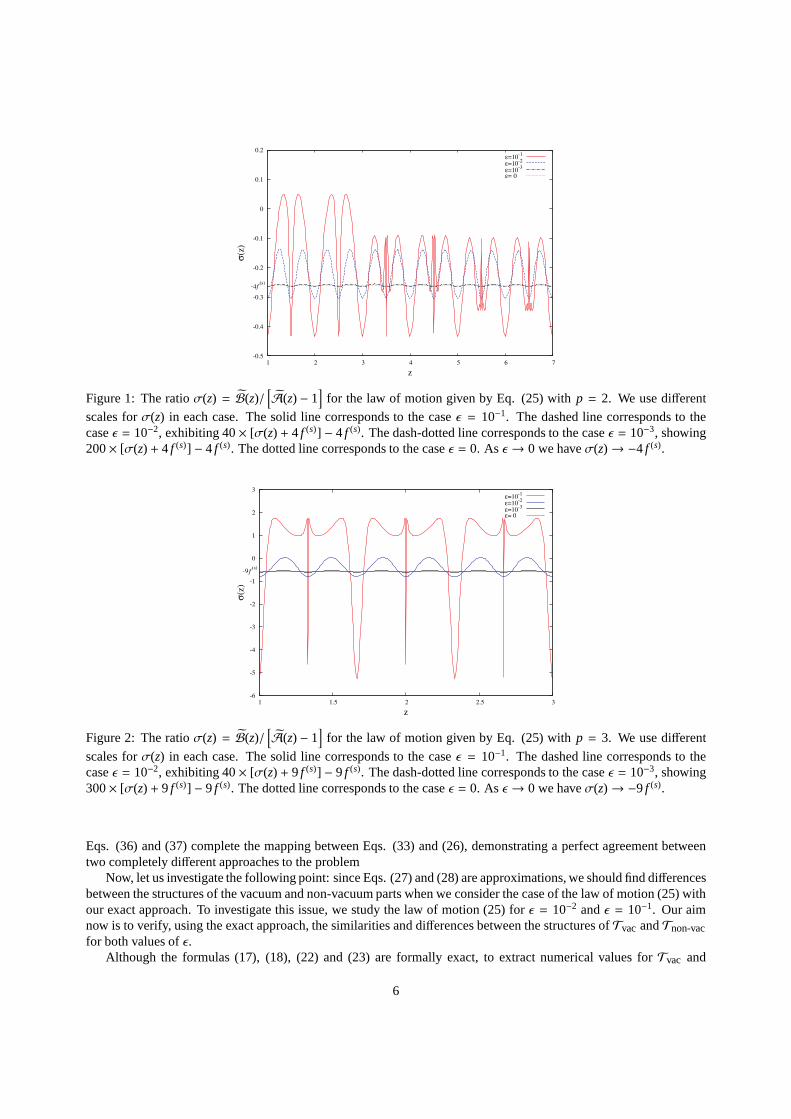
Figure 1: The ratioσ(z) = B(z)/[A(z) − 1

]for the law of motion given by Eq. (25) withp = 2. We use different

scales forσ(z) in each case. The solid line corresponds to the caseǫ = 10−1. The dashed line corresponds to thecaseǫ = 10−2, exhibiting 40× [σ(z) + 4 f (s)] − 4 f (s). The dash-dotted line corresponds to the caseǫ = 10−3, showing200× [σ(z) + 4 f (s)] − 4 f (s). The dotted line corresponds to the caseǫ = 0. Asǫ → 0 we haveσ(z)→ −4 f (s).

Figure 2: The ratioσ(z) = B(z)/[A(z) − 1

]for the law of motion given by Eq. (25) withp = 3. We use different

scales forσ(z) in each case. The solid line corresponds to the caseǫ = 10−1. The dashed line corresponds to thecaseǫ = 10−2, exhibiting 40× [σ(z) + 9 f (s)] − 9 f (s). The dash-dotted line corresponds to the caseǫ = 10−3, showing300× [σ(z) + 9 f (s)] − 9 f (s). The dotted line corresponds to the caseǫ = 0. Asǫ → 0 we haveσ(z)→ −9 f (s).

Eqs. (36) and (37) complete the mapping between Eqs. (33) and(26), demonstrating a perfect agreement betweentwo completely different approaches to the problem

Now, let us investigate the following point: since Eqs. (27)and (28) are approximations, we should find differencesbetween the structures of the vacuum and non-vacuum parts when we consider the case of the law of motion (25) withour exact approach. To investigate this issue, we study the law of motion (25) forǫ = 10−2 andǫ = 10−1. Our aimnow is to verify, using the exact approach, the similaritiesand differences between the structures ofTvac andTnon-vacfor both values ofǫ.

Although the formulas (17), (18), (22) and (23) are formallyexact, to extract numerical values forTvac and

6

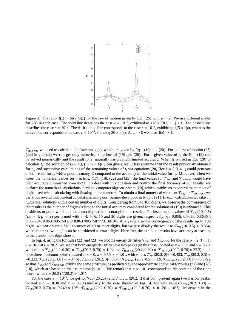
Figure 3: The ratioλ(z) = A(z)/s(z) for the law of motion given by Eq. (25) withp = 2. We use different scalesfor λ(z) in each case. The solid line describes the caseǫ = 10−1, exhibited as 1/6× [λ(z) − 1] + 1. The dashed linedescribes the caseǫ = 10−2. The dash-dotted line corresponds to the caseǫ = 10−3, exhibiting 1/5× λ(z), whereas thedotted line corresponds to the caseǫ = 10−4, showing 20× λ(z). As ǫ → 0 we haveλ(z)→ 1.

Tnon-vacwe need to calculate the functionsti(z), which are given by Eqs. (19) and (20). For the law of motion (25)(and in general) we can get only numerical solutions of (19) and (20). For a given value ofz, the Eq. (19) canbe solved numerically and the result fort1 naturally has a certain limited accuracy. Whent1 is used in Eq. (20) tocalculatet2, the solution oft2 + L(t2) = t1 − L(t1) can give a result less accurate than the result previously obtainedfor t1, and successive calculations of the remaining values ofti via equations (20) (fori = 2, 3, 4...) could generatea final result fortn with a poor accuracy, if compared to the accuracy of the initial value fort1. Moreover, when weinsert the numerical values forti in Eqs. (17), (18), (22) and (23), the final values forTvac andTnon-vaccould havetheir accuracy diminished even more. To deal with this question and control the final accuracy of our results, weperform the numerical calculations in Maple computer algebra system [20], which enables us to control the number ofdigits used when calculating with floating-point numbers. To obtain a final numerical value forTvac or Tnon-vac, wecarry out several independent calculations using our routines developed in Maple [21]. In each calculation we take allnumerical solutions with a certain number of digits. Considering from 3 to 100 digits, we observe the convergence ofthe results as the number of digits (related to the initial accuracy considered for the solution of (19)) is enhanced. Thisenable us to point which are the exact digits (the accuracy) in our results. For instance, the values ofTvac(10, 0.5)(L0 = 1, p = 2) performed with 3, 4, 5, 6, 10 and 20 digits are given, respectively by: 0.856, 0.8638, 0.86364,0.863704, 0.8637005768 and 0.86370057587773139184. Analyzing also the convergence of the results up to 100digits, we can obtain a final accuracy of 10 or more digits, butwe just display the result asTvac(10, 0.5) ≈ 0.864,where the first two digits can be considered as exact digits. Hereafter, the exhibited results have accuracy at least upto the penultimate digit shown.

In Fig. 4, using the formulas (22) and (23) we plot the energy densitiesTvac andTnon-vacfor the casep = 2,T = 1,ǫ = 10−2 at t = 20.2. We see that both energy densities have two peaks (in this case, located atx = 0.30 andx = 0.70,with valuesTvac(20.2, 0.30) = Tvac(20.2, 0.70) ≈ 1.94 andTnon-vac(20.2, 0.30) = Tnon-vac(20.2, 0.70)≈ 23.3), bothhave three minimum points (located atx = 0, x = 0.50,x = 1.01, with valuesTvac(20.2, 0)≈ −0.453,Tvac(20.2, 0.5)≈−0.322,Tvac(20.2, 1.01)≈ −0.461,Tnon-vac(20.2, 0)≈ 0.647,Tnon-vac(20.2, 0.5)≈ 1.9,Tnon-vac(20.2, 1.01)≈ 0.579),so thatTvac andTnon-vacexhibit the same structure, as predicted by the approximateanalytical formulas (27) and (28)[18], which are based on the assumption|ǫ| ≪ 1. We remark thatx ≈ 1.01 corresponds to the position of the rightmirror whent = 20.2 (L(20.2)≈ 1.01).

For the caseǫ = 10−1, we get forTvac(20.2, x) andTnon-vac(20.2, x) that both present again two narrow peaks,located atx = 0.30 andx = 0.70 (similarly to the case showed in Fig. 4, but with valuesTvac(20.2, 0.30) =Tvac(20.2, 0.70) ≈ 0.249× 1013, Tnon-vac(20.2, 0.30) = Tnon-vac(20.2, 0.70) ≈ 0.126× 1014). Moreover, in the

7

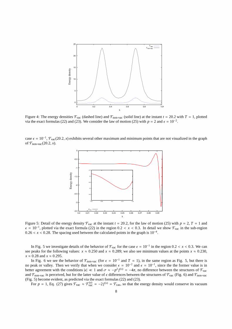
Figure 4: The energy densitiesTvac (dashed line) andTnon-vac(solid line) at the instantt = 20.2 with T = 1, plottedvia the exact formulas (22) and (23). We consider the law of motion (25) with p = 2 andǫ = 10−2.

caseǫ = 10−1, Tvac(20.2, x) exhibits several other maximum and minimum points that arenot visualized in the graphof Tnon-vac(20.2, x).

Figure 5: Detail of the energy densityTvac at the instantt = 20.2, for the law of motion (25) withp = 2, T = 1 andǫ = 10−1, plotted via the exact formula (22) in the region 0.2 < x < 0.3. In detail we showTvac in the sub-region0.26< x < 0.28. The spacing used between the calculated points in the graph is 10−4.

In Fig. 5 we investigate details of the behavior ofTvac for the caseǫ = 10−1 in the region 0.2 < x < 0.3. We cansee peaks for the following values:x ≈ 0.250 andx ≈ 0.289; we also see minimum values at the pointsx ≈ 0.230,x ≈ 0.28 andx ≈ 0.295.

In Fig. 6 we see the behavior ofTnon-vac (for ǫ = 10−1 andT = 1), in the same region as Fig. 5, but there isno peak or valley. Then we verify that when we considerǫ = 10−2 andǫ = 10−1, since the the former value is inbetter agreement with the conditions|ǫ| ≪ 1 andσ ≈ −p2 f (s) = −4π, no difference between the structures ofTvacandTnon-vacis perceived, but for the latter value ofǫ differences between the structures ofTvac (Fig. 6) andTnon-vac(Fig. 5) become evident, as predicted via the exact formulas(22) and (23).

For p = 1, Eq. (27) givesTvac ≈ T (a)vac = −2 f (s) = Tcas, so that the energy density would conserve its vacuum

8

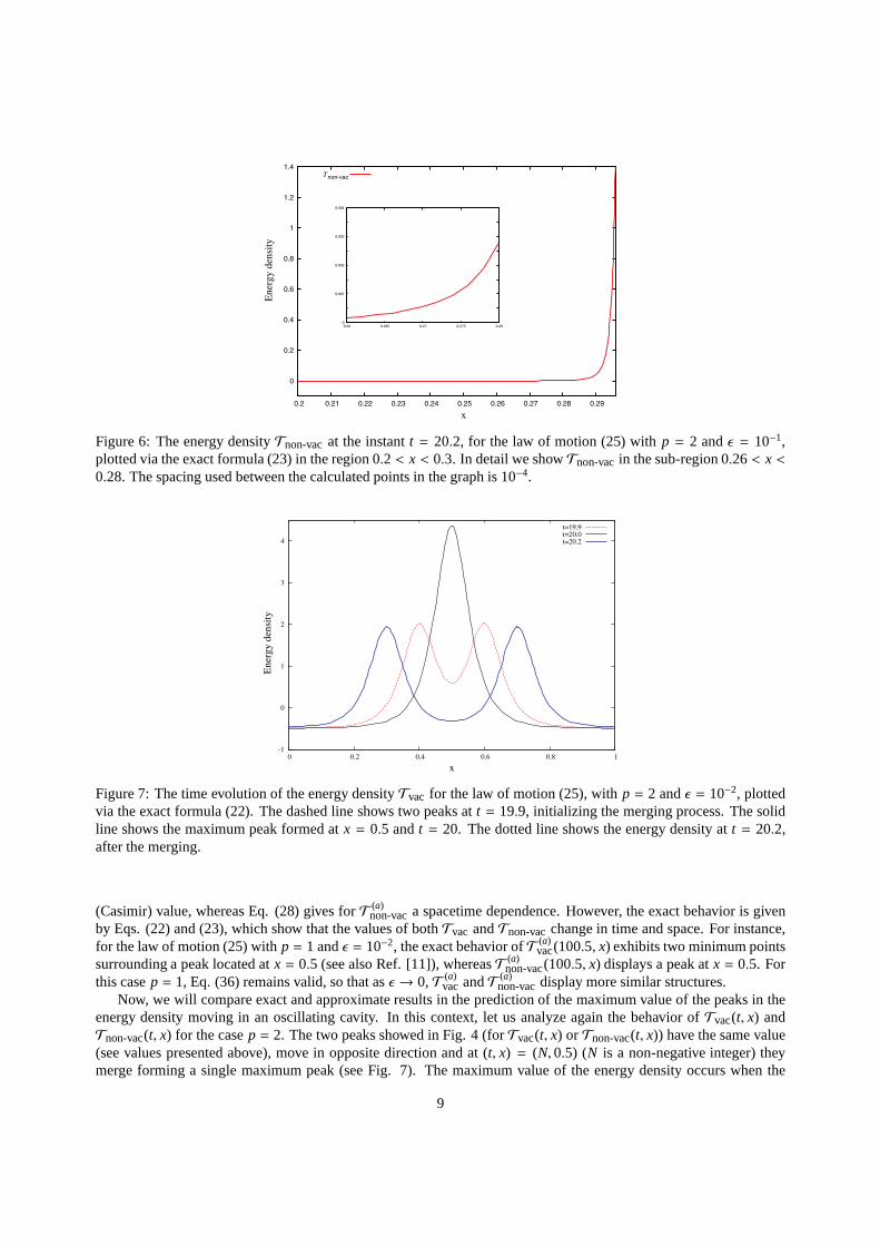
Figure 6: The energy densityTnon-vacat the instantt = 20.2, for the law of motion (25) withp = 2 andǫ = 10−1,plotted via the exact formula (23) in the region 0.2 < x < 0.3. In detail we showTnon-vacin the sub-region 0.26< x <0.28. The spacing used between the calculated points in the graph is 10−4.

Figure 7: The time evolution of the energy densityTvac for the law of motion (25), withp = 2 andǫ = 10−2, plottedvia the exact formula (22). The dashed line shows two peaks att = 19.9, initializing the merging process. The solidline shows the maximum peak formed atx = 0.5 andt = 20. The dotted line shows the energy density att = 20.2,after the merging.

(Casimir) value, whereas Eq. (28) gives forT (a)non-vaca spacetime dependence. However, the exact behavior is given

by Eqs. (22) and (23), which show that the values of bothTvac andTnon-vacchange in time and space. For instance,for the law of motion (25) withp = 1 andǫ = 10−2, the exact behavior ofT (a)

vac(100.5, x) exhibits two minimum pointssurrounding a peak located atx = 0.5 (see also Ref. [11]), whereasT (a)

non-vac(100.5, x) displays a peak atx = 0.5. Forthis casep = 1, Eq. (36) remains valid, so that asǫ → 0,T (a)

vac andT (a)non-vacdisplay more similar structures.

Now, we will compare exact and approximate results in the prediction of the maximum value of the peaks in theenergy density moving in an oscillating cavity. In this context, let us analyze again the behavior ofTvac(t, x) andTnon-vac(t, x) for the casep = 2. The two peaks showed in Fig. 4 (forTvac(t, x) orTnon-vac(t, x)) have the same value(see values presented above), move in opposite direction and at (t, x) = (N, 0.5) (N is a non-negative integer) theymerge forming a single maximum peak (see Fig. 7). The maximumvalue of the energy density occurs when the

9

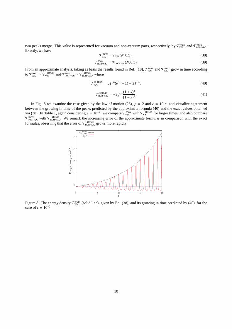
two peaks merge. This value is represented for vacuum and non-vacuum parts, respectively, byTmaxvac andTmax

non-vac.Exactly, we have

Tmaxvac = Tvac(N, 0.5), (38)

Tmaxnon-vac= Tnon-vac(N, 0.5). (39)

From an approximate analysis, taking as basis the results found in Ref. [18],Tmaxvac andTmax

vac grow in time accordingtoTmax

vac ≈ T(a)maxvac andTmax

non-vac≈ T(a)maxnon-vac, where

T (a)maxvac = 6 f (s)(e8τ − 1)− 2 f (s), (40)

T (a)maxnon-vac= −2g(s) (1+ κ)

2

(1− κ)2. (41)

In Fig. 8 we examine the case given by the law of motion (25),p = 2 andǫ = 10−2, and visualize agreementbetween the growing in time of the peaks predicted by the approximate formula (40) and the exact values obtainedvia (38). In Table 1, again consideringǫ = 10−2, we compareTmax

vac with T (a)maxvac for larger times, and also compare

Tmaxnon-vac with T (a)max

non-vac. We remark the increasing error of the approximate formulasin comparison with the exactformulas, observing that the error ofT (a)max

non-vacgrows more rapidly.

Figure 8: The energy densityTmaxvac (solid line), given by Eq. (38), and its growing in time predicted by (40), for the

case ofǫ = 10−2.

10

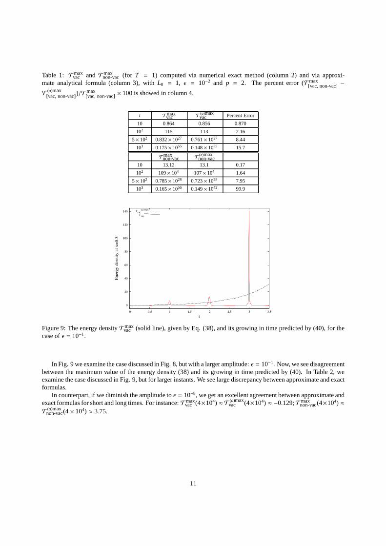
Table 1: Tmaxvac and Tmax

non-vac (for T = 1) computed via numerical exact method (column 2) and via approxi-mate analytical formula (column 3), withL0 = 1, ǫ = 10−2 and p = 2. The percent error (Tmax

[vac, non-vac]−T (a)max

[vac, non-vac])/Tmax[vac, non-vac]× 100 is showed in column 4.

t Tmaxvac T (a)max

vac Percent Error

10 0.864 0.856 0.870

102 115 113 2.16

5× 102 0.832× 1027 0.761× 1027 8.44

103 0.175× 1055 0.148× 1055 15.7

Tmaxnon-vac T (a)max

non-vac10 13.12 13.1 0.17

102 109× 104 107× 104 1.64

5× 102 0.785× 1028 0.723× 1028 7.95

103 0.165× 1056 0.149× 1042 99.9

Figure 9: The energy densityTmaxvac (solid line), given by Eq. (38), and its growing in time predicted by (40), for the

case ofǫ = 10−1.

In Fig. 9 we examine the case discussed in Fig. 8, but with a larger amplitude:ǫ = 10−1. Now, we see disagreementbetween the maximum value of the energy density (38) and its growing in time predicted by (40). In Table 2, weexamine the case discussed in Fig. 9, but for larger instants. We see large discrepancy between approximate and exactformulas.

In counterpart, if we diminish the amplitude toǫ = 10−8, we get an excellent agreement between approximate andexact formulas for short and long times. For instance:Tmax

vac (4×104) ≈ T (a)maxvac (4×104) ≈ −0.129;Tmax

non-vac(4×104) ≈T (a)max

non-vac(4× 104) ≈ 3.75.

11

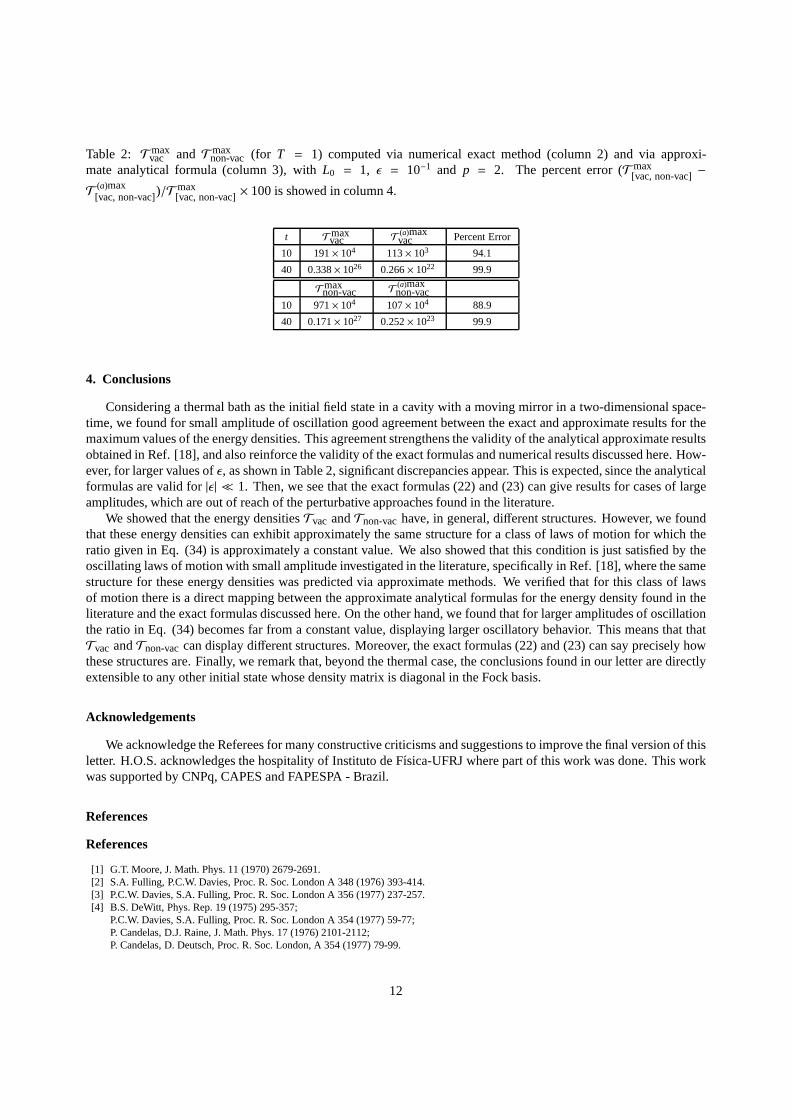
Table 2: Tmaxvac and Tmax

non-vac (for T = 1) computed via numerical exact method (column 2) and via approxi-mate analytical formula (column 3), withL0 = 1, ǫ = 10−1 and p = 2. The percent error (Tmax

[vac, non-vac]−T (a)max

[vac, non-vac])/Tmax[vac, non-vac]× 100 is showed in column 4.

t Tmaxvac T (a)max

vac Percent Error

10 191× 104 113× 103 94.1

40 0.338× 1026 0.266× 1022 99.9

Tmaxnon-vac T (a)max

non-vac10 971× 104 107× 104 88.9

40 0.171× 1027 0.252× 1023 99.9

4. Conclusions

Considering a thermal bath as the initial field state in a cavity with a moving mirror in a two-dimensional space-time, we found for small amplitude of oscillation good agreement between the exact and approximate results for themaximum values of the energy densities. This agreement strengthens the validity of the analytical approximate resultsobtained in Ref. [18], and also reinforce the validity of theexact formulas and numerical results discussed here. How-ever, for larger values ofǫ, as shown in Table 2, significant discrepancies appear. Thisis expected, since the analyticalformulas are valid for|ǫ| ≪ 1. Then, we see that the exact formulas (22) and (23) can give results for cases of largeamplitudes, which are out of reach of the perturbative approaches found in the literature.

We showed that the energy densitiesTvac andTnon-vachave, in general, different structures. However, we foundthat these energy densities can exhibit approximately the same structure for a class of laws of motion for which theratio given in Eq. (34) is approximately a constant value. Wealso showed that this condition is just satisfied by theoscillating laws of motion with small amplitude investigated in the literature, specifically in Ref. [18], where the samestructure for these energy densities was predicted via approximate methods. We verified that for this class of lawsof motion there is a direct mapping between the approximate analytical formulas for the energy density found in theliterature and the exact formulas discussed here. On the other hand, we found that for larger amplitudes of oscillationthe ratio in Eq. (34) becomes far from a constant value, displaying larger oscillatory behavior. This means that thatTvac andTnon-vaccan display different structures. Moreover, the exact formulas (22) and (23) can say precisely howthese structures are. Finally, we remark that, beyond the thermal case, the conclusions found in our letter are directlyextensible to any other initial state whose density matrix is diagonal in the Fock basis.

Acknowledgements

We acknowledge the Referees for many constructive criticisms and suggestions to improve the final version of thisletter. H.O.S. acknowledges the hospitality of Instituto de Fısica-UFRJ where part of this work was done. This workwas supported by CNPq, CAPES and FAPESPA - Brazil.

References

References

[1] G.T. Moore, J. Math. Phys. 11 (1970) 2679-2691.[2] S.A. Fulling, P.C.W. Davies, Proc. R. Soc. London A 348 (1976) 393-414.[3] P.C.W. Davies, S.A. Fulling, Proc. R. Soc. London A 356 (1977) 237-257.[4] B.S. DeWitt, Phys. Rep. 19 (1975) 295-357;

P.C.W. Davies, S.A. Fulling, Proc. R. Soc. London A 354 (1977) 59-77;P. Candelas, D.J. Raine, J. Math. Phys. 17 (1976) 2101-2112;P. Candelas, D. Deutsch, Proc. R. Soc. London, A 354 (1977) 79-99.

12

[5] V.V. Dodonov, J. Phys.: Conf. Ser. 161 (2009) 012027-1-012027-28;V.V. Dodonov, arXiv:1004.3301v1 (2010);D.A.R. Dalvit, P.A. Maia Neto, F.D. Mazzitelli, arXiv:1006.4790v2 (2010).

[6] C. Braggioet al, Europhys. Lett. 70 (2005) 754-760;A. Agnesiet al, J. Phys. A: Math. Theor. 41 (2008) 164024-1-164024-7;A. Agnesiet al, J. Phys.: Conf. Ser. 161 (2009) 012028-1-012028-7.

[7] J.R. Johansson, G. Johansson, C.M. Wilson, F. Nori, Phys. Rev. Lett. 103 (2009) 147003-1-147003-4;C.M. Wilsonet al, arXiv:1006.2540v1 (2010);J.R. Johansson, G. Johansson, C.M. Wilson, F. Nori, arXiv:1007.1058v1 (2010).

[8] C.K. Law, Phys. Rev. Lett. 73 (1994) 1931-1934;Y. Wu, K. W. Chan, M.C. Chu, P.T. Leung, Phys. Rev. A 59 (1999) 1662-1666;P. Wegrzyn, J. Phys. B 40 (2007) 2621-2640.

[9] V.V. Dodonov, A.B. Klimov, and D. E. Nikonov, J. Math. Phys. 34 (1993) 2742-2756.[10] D.A.R. Dalvit, F.D. Mazzitelli, Phys. Rev. A 57 (1998) 2113-2119.[11] C.K. Cole, W.C. Schieve, Phys. Rev. A 52 (1995) 4405-4415.[12] C.K. Cole, W.C. Schieve, Phys. Rev. A 64 (2001) 023813-1-023813-9.[13] L.H. Ford, A. Vilenkin, Phys. Rev. D 25 (1982) 2569-2575;

P.A. Maia Neto, J. Phys. A 27 (1994) 2167-2180;P.A. Maia Neto, L.A.S. Machado, Phys. Rev. A 54 (1996) 3420-3427;P.A. Maia Neto, L.A.S. Machado, Braz. J. Phys. 25 (1996) 324-334;B. Mintz, C. Farina, P.A. Maia Neto, R.B. Rodrigues, J. Phys.A: Math. Gen. 39 (2006) 6559-6565;B. Mintz, C. Farina, P.A. Maia Neto, R.B. Rodrigues, J. Phys.A: Math. Gen. 39 (2006) 11325-11333.

[14] M. Razavy, J. Terning, Phys. Rev. D 31 (1985) 307-313;G. Calucci, J. Phys. A 25 (1992) 3873-3882;C.K. Law, Phys. Rev. A 49 (1994) 433-437;V.V. Dodonov, A.B. Klimov, Phys. Rev. A 53 (1996) 2664-2682;D.F. Mundarain, P.A. Maia Neto, Phys. Rev. A 57 (1998) 13791390;D.T. Alves, C. Farina, E.R. Granhen, Phys. Rev. A 73 (2006) 063818-1-063818-8;J. Sarabadani, M.F. Miri, Phys. Rev. A 75 (2007) 055802-1-055802-4.

[15] M.-T. Jaekel, S. Reynaud, J. Phys. I (France) 3 (1993) 339-352;M.-T. Jaekel, S. Reynaud, Phys. Lett. A 172 (1993) 319-324;L.A.S. Machado, P.A. Maia Neto, C. Farina, Phys. Rev. D 66 (2002) 105016-1-105016-12;D.T. Alves, C. Farina, P.A. Maia Neto, J. Phys. A 36 (2003) 1133311342;D.T. Alves, E.R. Granhen, M.G. Lima, Phys. Rev. D 77 (2008) 125001-1-125001-5 .

[16] V.V. Dodonov, J. Phys. A: Math. Gen. 31 (1998) 9835-9854;G. Plunien, R. Schutzhold, G. Soff, Phys. Rev. Lett. 84 (2000) 1882-1885;J. Hui, S. Qing-Yun, W. Jian-Sheng, Phys. Lett. A 268 (2000) 174-177;R. Schutzhold, G. Plunien, G. Soff, Phys. Rev. A 65 (2002) 043820-1-043820-15;G. Schaller, R. Schutzhold, G. Plunien, G. Soff, Phys. Rev. A 66 (2002) 023812-1-023812-20.

[17] V.V. Dodonov, A. Klimov, V.I. Man’ko, Phys. Lett. A 149 (1990) 225-228;D.A.R. Dalvit, P.A. Maia Neto, Phys. Rev. Lett. 84 (2000) 798-801;V.V. Dodonov, M.A. Andreata, S.S. Mizrahi, J. Opt. B: Quantum Semiclass. Opt. 7 (2005) S468-S479.

[18] M.A. Andreata, V.V. Dodonov, J. Phys. A 33 (2000) 3209-3223.[19] D.T. Alves, E.R. Granhen, H.O. Silva, M.G. Lima, Phys. Rev. D 81 (2010) 025016-1-025016-10.[20] www.maplesoft.com[21] D.T. Alves, E.R. Granhen,The Dynamical Casimir package, paper in preparation.

13