CONVENTIONAL RF CAVITY DESIGN

M. Puglisi Sincrotrone Trieste, Trieste, Italy

ABSTRACT The theory of ideal cavity resonators is outlined with rigourous definitions for the modes and their most important parameters. Analytical formulas are obtained for calculating the fields and the resonant frequencies of the cavities, derived from the lossless uniform tri-rectangular and cylindrical waveguides. The concept of equivalent circuits is introduced while the theory of periodic structures is outlined. Attention is given to cavities derived from the uniform coaxial line, together with an outline of the method to evaluate the losses and some sketches of the feeding systems.

1. INTRODUCTION

In electrodynamic accelerators, with the notable exception of the betatron, the energy is delivered to the particles by means of a large variety of devices normally known as cavity resonators. From the dawn of the age of the electrodynamic accelerators (1931, the cyclotron of E.0. Lawrence at Berkeley) to the present day, both the theory and the technology of these devices have undergone a tremendous development. Yet new and important innovations are still to be expected in this field as a consequence of the continuous demand for better performance that, in tum, follows and conditions the progress of accelerators. A historical record of this rapid development can be found by looking at the many names with which these devices have been, and currently are, known, i.e., cavity, resonant cavity, RF cavity, klystron cavity, reentrant cavity, coaxial cavity, quarter-wave cavity, foreshortened coaxial cavity, foreshortened quarter-wave cavity, folded cavity, pill-box cavity, hollow cavity, holrhaum.

Even though the development of the cavity resonator has been strongly influenced by the needs of the particle accelerators it is also true that these devices find a large variety of applications in the field of the electrical communications and, in general, in those applications where the distinctive characteristic of the cavity is used, i.e., to contain in a limited volume a standing electromagnetic field. This means that a cavity is an electromagnetic device that must not radiate. Consequently it is clear that a volume of perfect dielectric totally limited by perfectly conducting walls is a good operative definition of an ideal cavity. In fact a wave can travel indefinitely inside its dielectric through an endless number of reflections at the walls without suffering any loss, i.e., a standing electromagnetic field can be 'contained' inside the device. Alternatively we could conclude that if a cavity contains a standing field this field could not be detected from the outside. Consequently, a charged particle that comes from the outside and enters the cavity would experience the field only at the last moment inside the cavity. Then a net exchange of energy between field and particle would be perfectly possible, even if the particle travelled along a closed orbit including the cavity.

2. THE MATHEMATICAL THEORY OF THE IDEAL CAVITY

The ideal cavity is defined as a volume of perfect dielectric limited by infinitely conducting walls. Moreover a dielectric is perfect if, and only if, it is linear, isotropic, time invariant and lossless. When the above conditions are met, the mathematical theory becomes very simple but its application to the physical cases becomes very difficult. In fact we should expect that the introduction of losses would modify drastically the theory of the lossless case.

156

On the other hand the theory of a real cavity is very complicated. For instance, the walls must contain many 'openings' towards the outside (the coupling holes) and one should take into account the fact that the 'volume' of the cavity must be extended even to infinity (induction and radiation effects).

Fortunately, if we assume that the dielectric has a finite conductivity crd while the walls remain perfectly conducting, then we obtain the case of the 'ideal' but lossy cavity. This is extremely important sipce the result obtained from a simple and elegant mathematical treatment can be immediately extended to the most general case.

Let e = e(x,y,z,t) and h = h(x,y,z,t) be the electric and magnetic fields that at any instant fill the volume V of the cavity. The dielectric is characterized by the three constants: the electrical permittivity E, the magnetic permittivity µ and the conductivity crd. Moreover we assume that inside the cavity both the charge density and the induced currents are equal to zero. Consequently the Maxwell equations can be written as follows:

V · e=O

V · h=O

dh V xe=-µ-

dt (1)

We notice that Jd = crde is the conduction current inside the dielectric that is responsible for the losses in this case. If crd tends to zero then the lossy cavity tends to the ideal one.

Taking the curl of both sides of the third equation and substituting Vxh obtained from the fourth we obtain:

(2)

For a generic vector A the following identity holds:

VxVxA = V V·A - V2A (3)

where V2 indicates the vector Laplace operator. Using the identity (3) and taking into account that V·e = 0, Eq. (2) becomes:

(4)

which is the famous equation of the electromagnetic waves inside a linear homogeneous time invariant and conducting medium in the absence of both free charges and impressed currents.

The wave equation can be solved only when the boundary conditions are given, and in our case where 'the volume V is limited by perfectly conducting walls' the boundary conditions are:

(5)

where n is the versor of the normal to the boundary, oriented towards the inside of the volume.

157

From the mathematical theory of the linear operators we know that the vector eigenfunction:

E = E(x,y,z) (6)

satisfying the conditions:

(

2 2 V E+A E=O

V · E = 0 in the volume n x E = 0 on the boundary

(7)

exists for an infinite discrete set of real values for the parameter A. It is also well-known that the set constitutes a complete basis for representing any divergenceless field perpendicular to the boundary. Moreover, we recognize that the boundary conditions that define expression (7), and the boundary conditions that are appropriate to solve the wave equation, are exactly the same. Consequently, if the couple En, An satisfies (7) for the volume of the cavity, we can write:

e(x,y,z,t) =I, an(t) En n

(8)

where the an(t) are functions, unknown, of time only, and each of the En (which are functions of the coordinates only) satisfies the boundary conditions.

To find the an= an(t) we substitute the expansion (8) into the wave equation (4) and obtain:

(9)

Again making use of the solution of (7) we can write:

(10)

and substituting into Eq. (9) we obtain:

Factorizing the vector functions En we obtain:

2:{An2 an(!) + µ<rd gt an(!) + Eµ ;~ •n(I)} E,, ~ 0 · (12)

At this point we immediately recognize that Eq. (12) has a non-trivial solution if, and only if, each term of the summation is zero. This fact determines the form of the an(t).

In fact the condition:

(13)

158

means that for each an we must have:

(14)

where:

2E t=-

crd

n.=~ / 1-! [crd ~]2 ,.,;;;;. ~ 4 E An =con-n 2

4Qn

A 1 and A2 are integration constants which depend upon the initial distribution of the fields inside the cavity

(15)

When crd tends to zero then t and On tend to infinity while On tends to eon.

So far we have restricted ourselves to the problem of the undriven ideal, but lossy, cavity. In other words we are considering a lossy device in which some electromagnetic energy has been stored only at the time t = to (the initial conditions) whereas the presence of the attenuation factor exp(-t/t) tells us that the energy is disappearing with time.

Now, although we treated a particular case, many important and general conclusions can be derived, in particular:

i)

ii)

iii)

iv)

v)

vi)

The electric field inside an undriven lossless cavity is made up of the sum of standing fields each of which has form and frequency respectively defined by a couple eigenfunction + eigenvalue of the set.

Each function En = En(x,y ,z) defines a resonant mode whose resonant frequency is Vn = con/21C = An/21C ...feµ.

Each mode satisfies the geometric boundary conditions. The time dependency of the amplitude of each mode is sinusoidal exponentially damped if crd '# 0.

The quality factor Cb is a dimensionless quantity that depends upon both the resonant frequency and the time constant of the mode.

For crd = 0 the energy stored in each mode must remain constant and consequently the amplitude An of the mode cannot change. This means that when the instantaneous value of the electric field is zero then all the energy of the mode must be stored in the magnetic field whose instantaneous value, at that moment, must reach the peak. We conclude that the electric and the corresponding magnetic fields of each mode oscillate in time quadrature.

If the quality factor Qi of a mode is less than 1/2 then the mode still exists but its amplitude vanishes exponentially with time without oscillations.

159

3. THE REAL CAVITY

In a real cavity the dielectric does not represent, in general, the most important cause of losses. Conversely, the conductivity er of the metallic walls is not infinite and consequently a large fraction of the exciting power is wasted by the Joule effect on the non-perfectly conducting boundaries. (This means that the condition n x E = 0 on the boundary is no longer applicable.) Moreover the cavity is equipped with many electrical devices that are not exempt from losses (coupling inductors and capacitors, tuners, dielectric coupling windows, parasitic­mode suppressors, connections to the vacuum system and special probes). In addition to these intrinsic causes of losses, the cavity can be used for transmitting energy to a load that, in our case, is always a beam of charged particles. Consequently, any attempt to obtain a rigourous solution of the problem of the cavity renders the theory so complicated that in every treatment there is a point where some simplifying hypotheses are introduced (openly or rather covertly).

With this in mind many authors prefer to circumvent the difficulty by defining the quality factor of the cavity using the complex form of the Poynting vector as will be shown in the following. Certainly, it is well-known that the use of this vector postulates that the time variations of the considered fields are determined by complex exponentials. But this is what we have found to be exactly true for the cavity loaded only by the dielectric and, for this reason, we assume that the same thing should happen for any of the possible linear loads.

3. 1 The complex form of the Poynting vector

We assume that the electric and magnetic fields together with the current density can be written as follows:

A = A(x,y,z) e(-a+jro)t (16)

where A stands for a generic vector that depends upon the coordinates only while a and ro are constants. The Maxwell equation then becomes:

V·E=O

V·H=O

V x E =-(-a+ jro)µH

v x H = J + (-a + jro )EE •

(17)

If P = E x H* is the complex Poynting vector, using a well-known vector identity we can write:

V·P = V·(E x H*) = H*·V x E- E·V x H*. (18)

Because the conjugate of the product of two complex quantities is equal to the product of their conjugates we have:

V x H* = J* +(-a - jro) EE*. (19)

Substituting into Eq. (18) the VxE from the third of the expression (17) and the expression of VxH* given by (19) we obtain for the power density P:

-V·P = E·J* - a(µ IHl2 + £ IEl2) + jro (µ IHl2 - £ IEl2). (20)

This equation can be integrated over the volume V of the cavity and, taking into account the divergence theorem, we obtain:

160

_ _!_ J P·ds = _!_ f E·J* dV - 2a (UH+ Up)+ 2jco(UH- Up) 2 s 2 v (21)

where the left hand side term is the inward flux of the complex Poynting vector (complex power entering the cavity).

The first term of the right hand side is the absorbed complex power. If we assume that J = crE then:

1 f 1 f 2 - E·J* dV = - O' IEI dV = w 2 v 2 v

(22)

becomes the power wasted in the dielectric and in the walls of the cavity [cr = cr(x,y,z)] *).

With UH and VE we have indicated the average electric and the average magnetic energies respectively stored in the dielectric. If now we assume that the cavity is not fed from the outside, and taking into account (22) we obtain:

w -2a <UH+ UE) + 2jco (UH - UE) = 0 .

Equating the real and imaginary parts we obtain:

{W= 2a (UH+ Up)

UH=UE

From the first expression of (24) we obtain:

(23)

(24)

(25)

It is now evident that 1/a has the same meaning and plays the same role as the time constant t defined by (15) together with the quality factor Qi. Consequently we generalize the definition of the quality factor writing:

(26)

Substituting the value of a we obtain:

(27)

where Vn = l{f n is the resonant frequency of the mode not perturbed by the losses.

Since the product W·Tn represents the energy wasted per cycle, it follows that (27) can be reformulated in a very general fonn:

Qn _ 2

Energy stored - 7t Energy dissipated per cycle ·

*) This formula takes into account both the losses in the dielectric and in the conducting walls. Consequently, the conductivities to be considered are that of the dielectric and that of the metallic walls.

161

3. 2 Quality factor, shunt impedance and related topics

From the definition (15) and its physical meaning (27) we have seen that the quality factor is a dimentionless quantity, uniquely defined for each mode, which together with the resonant frequency completely defines the behaviour of the undriven cavity. In fact, apart from the initial conditions, the amplitude An of a considered mode depends upon the differential equation:

(28)

where we have only two constants: the quality factor and the radian resonant frequency of the mode not perturbed by the losses.

We also note that the definition of quality factor given by (27) is very general and consequently takes into account the effect of any kind of linear losses that may load the considered mode. Conversely, it should be noted that the quality factor is characterized by the ratio of energies and consequently cannot give any idea about the amount of power that should be needed to maintain constant the amplitude of a mode inside a driven cavity.

The parameter that should tell us about the power required to maintain constant the amplitude of a mode is the shunt impedance of the mode (we note that in spite of the name the shunt impedance is always a real quantity). Unfortunately, the shunt impedance cannot be uniquely defined simply because the amplitude of a mode depends upon the point selected for measuring it. Moreover the shunt impedance should be related to the idea of the 'voltage' associated with a mode. Here again we meet an ambiguity because inside the cavity VxE cannot be zero and consequently the voltage between two points depends upon the chosen integration path. However, the purpose of the cavity usually determines that integration path is more convenient for the specific case.

In our case the cavities are made for exchanging energy with the charged particles and have axial symmetry. Therefore, the axis of the cavity is normally chosen for evaluating the line integral that defines the gap voltage Va and we define:

(29)

where IEzl is the modulus of the z component of the electric field along the axis and h is that portion of the axis where the electric field is effective. (Normally h is somewhat longer than the geometrical length of gap.)

Note that the above definition does not coincide with the voltage gained by a charged particle that travels along the gap explained in the previous chapter of these proceedings. Once the 'voltage' produced by the cavity is defined then the shunt impedance becomes:

V'f:, Rsh = 2 p (30)

where P is the real power needed for maintaining the voltage VG· The factor two that appears in (30) is fundamental because, as we have already seen, the amplitude of each mode depends sinusoidally upon the time. Nevertheless sometimes, and particularly in the literature concerning linacs, this factor is omitted. Consequently, the reader is strongly advised to be sure of the conventions adopted in the different treatments.

162

Having defined the shunt impedance then, using the definition of the quality factor, it is possible to define the equivalent capacity 'Ceq' of the mode. Substituting into (27) the physical quantities already defined we obtain:

1 2 2 Ceq V 0 Qo = 27t = coo Rsh Ceq

1 v'{, 1 2 Rsh Vo

C = Qo eq coo Rsh

(31)

where Qo and coo are respectively the quality factor and the resonant frequency of the considered mode.

Note particularly that the differential equation for the voltage obtained by the shock excitation of a parallel R,L,C circuit becomes exactly equivalent to (28) if we assume:

R = Rsh ; C = Ceq ; L = RshQ coo

(32)

Consequently the parameters defined by (32) are known as the equivalent parameters of a mode.

4. CAVITIES DERIVED FROM UNIFORM TRANSMISSION SYSTEMS

4. 1 Introduction

The most common energy transmission systems are the uniform transmission line and the rectangular or circular uniform waveguide. Both these systems are widely used in the communication engineering and an enormous amount of literature can be found on them. While some important formulas will be given in the following paragraphs here we concentrate our attention on the fact that both the systems, if lossless, can suppon without attenuation travelling electromagnetic waves with sinusoidal time variation and constant phase velocity Vp· This means that any component of the fields that constitute the wave can be W!itten as a function of the coordinates in the transverse plane multiplied by a phase factor eJ(rot-~z) that takes into account both the time and the z dependency. In communication engineering the phase constant is indicated with the Greek letter p that in the 'accelerator's idiom' universally indicates the normalized velocity of a particle and the amplitude of the betatron functions. 1bis is a fact of the life and because the risk of possible confusion is very little we suggest to use the P with the different meanings. It is imponant to recognize that Pz is the phase advance of the wave as it travels along the distance z, and that, by definition, the wave length Ag is the minimum distance between two points with the same phase and at the same value of time. Consequently at any moment:

PA.g = 2 7t. (33)

If v = co/27t is the frequency, T = l/v the time period of the fields, and vp is the phase velocity, then:

v Ag = Vp T = ..:Q v

27t co p - - - -· - VpT - Vp'

(34)

it being very imponant to avoid confusion between the free space wavelength A and the propagation wavelength Ag.

163

The important point is that the phase velocity of the electromagnetic wave in free space is equal to the speed of the light c in vacuum. However, inside the transmission system the situation may be different:

i) The dielectric that is inside the transmission system and thus supports the fields may have electric and magnetic relative permeabilities (Er, µr) different from 1.

ii) The propagation inside a bounded medium may demand a phase velocity that is different

from c~ as will be seen later on.

Here we anticipate that in a smooth wave guide the phase velocity is always larger than the one that can be measured, at the same frequency, in the unbounded dielectric that fills the guide.

Now we consider two waves where the corresponding fields have the same amplitudes but travel in opposite directions. If Vis the common amplitude of one component, then the resulting amplitude VR of this component along the propagation system becomes:

VR =Re { V e.i<mt-lh) + V ei(rot+~z)} = 2 V cosrot cosJ3z . (35)

We see that a purely standing wave has been set up where, for any value of time, the minimum distance between two points of 'maximum' or two points of 'null' is always equal to Ag!l. This simple consideration leads to the realization of cavity resonators that can be derived from a uniform transmission system. In fact, if a uniform transmission system can support a travelling wave with a wavelength equal to Ag at the radian frequency co, then a 'stub' of this system limited by two short circuiting planes separated by the distance:

A d = p y p = 1,2,3,... (36)

constitutes a cavity that at the same radian frequency 'contains' a standing wave, i.e., a resonant cavity.

It is important to stress that the cavity already indicated can resonate at all the frequencies that fulfill Eq. (36) and, if consistent with the boundary conditions, at all the frequencies for which Ag= oo or, stated differently J3 = 0.

In the field of accelerators the form of the required fields and their resonant frequencies are the known or assigned parameters and consequently a suitable 'supporting' cavity must be found. This means that the modes allowed by the uniform transmission should be investigated.

4. 2 Uniform waveguides

A uniform waveguide is defined as a dielectric volume limited by conducting cylindrical walls. Two important cases are normally considered:

a) Rectangular cross section. b) Circular cross section.

Moreover we limit ourselves to the case of the lossless waveguides.

Let us indicate with T the coordinate of the cross section (x,y and r,<I> for the cases a and b respectively). H 'Jf{T) indicates any real function of the transverse coordinates then:

E \ _ (T) j(rot - ~z) Hf='Jf e (37)

164

indicates a sinusoidal field that propagates along the z axis with phase velocity vp equal to co/13 where 13 is a real function of co that for the moment is unknown.

If the above fields are substituted into the Maxwell equations we obtain a linear system where the transverse fields depend upon the derivatives of the longitudinal fields. Solving the system we obtain:

Rectangular Coordinates Cylindrical Coordinates

where (38)

From the above equations it is evident that:

(39)

where with V1 we indicate the gradient operator in the transverse plane.

It is now evident that our problem is solved when we know the longitudinal components Ez and Hz and the value of kc. Before proceeding with this determination we recognize that:

i) The solutions Ez and Hz are obviously independent. From the systems (38) we see that the total field in the guide may depend upon both the Ez and Hz functions.

ii) The fields for which Hz= 0 are called transverse magnetic (TM) modes (accelerating modes), while the fields for which Ez = 0 are the transverse electric (TE), deflecting, modes.

The scalar potentials Ez. Hz together with the corresponding values of kc, are obtained as follows:

We indicate by Va vector that can represent either E or H, and from the Maxwell equations we obtain the familiar vector wave equation:

a2v V2 v = + Eµ 2 dt2 .

For the z component we obtain (in both the coordinate systems):

t72 a2vz a2v z v T V z + az2 = + Eµ dt2

where V.j. indicates the scalar bidimensional (transverse) Laplacian operator. Introducing the general hypothesis (1) we obtain the fundamental equation:

V.j. Vz + (ro2eµ - ~2) Vz = 0 or

165

(40)

From the mathematics we know that given the appropriate boundary conditions this equation can be solved for an infinite number of discrete real values of kc (the eigenvalues) to that correspond an infinite number of eigenfunctions.

y

b

a x

.... z

Fig. 1 Cross sections and reference systems for rectangular and circular waveguides

With reference to Fig. 1, we obtain:

Cartesian

E Eo . m1t . n7t

z= smax smby m7t mt

Hz =Ho cos ax cos by

Cylindrical

Pv1 forEz a

k -c- P'v1 for Hz a

(41)

where m,n and v ,1 are couples of arbitrary integers, Iv is the Bessel function of order v, Pv1 and P'v1 are respectively the Ith root of the Bessel function of order v and the Ith root of its derivative.

From Eq. (41) we know the possible form for the longitudinal fields and the corresponding values of the eigenvalues kc. Recalling that kc is related to the phase constant P we obtain:

p = ± i1t = -Vro 2Eµ - k~. g

(42)

It is now clear that because kc is always real then the propagation in a waveguide is always possible (i.d. p is real) above certain 'cut-off frequencies that depend upon the chosen mode of propagation (choice between TE or TM modes and choice of the integers m,n or v ,1 according to the cross section of the guide). Moreover since w2Eµ must be larger than ~ then

Ag must be larger than A.. Consequently the phase velocity vp must be larger than 1f'.[ql..

166

At this point the theory has been developed to the point where we can understand how a stub of waveguide can work as a resonant cavity. In fact as soon as the following parameters are given:

1) the cross section of the guide, 2) the guide mode of operation, 3) the number p of half-wavelengths included, 4) the working (resonant) frequency,

then the axial length 'd' of the cavity that is derived from the guide and fulfills the above requirement should be:

(43)

As before, the case p = 0 is meaningless and cannot be considered whereas the condition f3 = 0 leads to the equation:

(44)

This means that given a possible value for kc. in the m,n or v ,1 mode, this mode can resonate in a cavity of any length provided that the boundary conditions are also satisfied on the shorting planes. (For instance, a TE mode would not fit the boundary condition on the shorting planes for the case of a circular waveguide.)

5 . THE PERIODIC STRUCTURES

We have already seen that the phase velocity of a wave in an empty and uniform waveguide is always larger than the speed of light so that a TM wave propagating along a uniform guide could never be synchronous with any charged particle even if ultra-relativistic. On the other hand it is immediately evident that if a uniform system can propagate a wave along

its z-axis with a phase velocity less than llV Eo µo then its kc2 should be less then zero. In fact, with reference to Cartesian or cylindrical coordinates and indicating with Tone of the couples x,y or r,<I>, we assume that:

. 21t ·J-Z

Ez = E(T,z) = E(T) e Ag (45)

is the z-component of an electric field that travels along the system with phase velocity less than c and consequently Ag < A..

Substituting into the wave equation we obtain:

2 2 VT E (T) + kc E (T) = 0 (46)

and the value of kc2 turns out to be negative. But if kc2 < 0, the eigenfunctions become sinusoidal or Bessel functions of imaginary argument that have no zeros and are monotonic. Consequently, the boundary conditions dictated by a uniform waveguide cannot be satisfied. However, what is impossible for uniform waveguides, is perfectly possible if the boundary conditions of the waveguide are not uniform, i.e., if the guide is corrugated.

A periodic structure is a device with a straight axis (normally the z or propagation axis) whose geometry repeats itself with period L along the z axis. Although a periodic system can be realized in very many different ways, from now on we will represent such devices by a

167

corrugated waveguide as indicated in Fig. 2. However, it should be clear that instead of thinking only in terms of a corrugated waveguide, it is perfectly correct to assume that this periodic structure can be made by cascading a series of pill-box cavities coupled through circular holes centered on the axis.

I

1a I

•a I

Fig. 2 Axial and normal sections of a corrugated waveguide

0

The situation indicated in Fig. 2 can be transformed in many ways. For instance stretching the thickness of each 'washer' we obtain the structure shown in Fig. 3. In this example the coupling between adjacent cavities is obtained via loops because, in general, a drift tube could not give enough coupling. (A drift tube can be schematized as an element of uniform waveguide well below the cut-off for the whole range of operating frequencies).

Fig. 3 Axial section of a periodic structure made with cavities and drift tubes

Many other useful periodic structures have been invented and there are good reasons to expect that new devices will be devised in the near future.

The theory of the periodic structures is very complicated and outside the scope of this lecture. Nevertheless, some simple considerations may cast some light on the topic.

S .1 Space harmonics

The most important theorem for use in understanding the behaviour of the periodic structures can be formulated as follows: 'If an electromagnetic mode, that depends sinusoidally on time, propagates itself along a periodic structure that has period L, then the fields in two sections, distant L, are equal within a complex constant'. This statement, which is a simplified

168

_,... z

version of the Floquet*> theorem, can be intuitively demonstrated taldng into account that when the mode travels along the structure, in a steady state situation, then the whole structure could be shifted by one period along the axis and an observer could detect only a change in the complex phase of the fields.

Let us assume that the propagation is along the z axis of the structure that coincides with the z axis of the chosen system of coordinates. Moreover we drop, as usual, the factor eicot where co is the radian frequency of the fields. The form of any component of the mode in the structure can now be written as:

E = E (T,z) e-yoz (47)

where Yo is constant and can be complex and, most important, E is a periodic function of z with period equal to 'L'.

It is immediately clear that Eq. (47) agrees with the Floquet theorem. In fact let E1 and Bi be the values of the component, for the same transverse coordinates, in the two corresponding sections that have the abscissa z1 and z2 = z1 + L. From (47) we have:

f E1 = E (T,z1) e-1oz1

\ E2=E(T,zi)e-1oz2=E(T,z1+L)e-Yo(z1+L)=E(T,z1)e-Yoz1. e-YoL

and the Floquet theorem is satisfied.

It is intuitively evident that if the structure is lossless then the constant 'Yo cannot be complex and must be either imaginary (propagation) or purely real (attenuation). In the following we assume that we are dealing with 'propagation' along lossless structures and consequently y = j Po, where Po is a real quantity that depends upon the frequency of the wave.

The assumption made in Eq. (47) can be exploited taldng into account that the function E must be periodic with period equal to L and, in fact, we can write:

+oo ~ .21tn

E (T,z) = £..- En<n e-JL z

(48)

where the origin of each cell can be arbitrarily defined.

The function E = E (T,z) is supposed to match the boundary conditions imposed by the cell while the functions En = En (T) cannot since they are independent of z.

Substituting the expansion (48) into (47) we obtain:

*) This is a well-known mathematical theorem. A complete treatment of the whole topic can be found in reference [6].

169

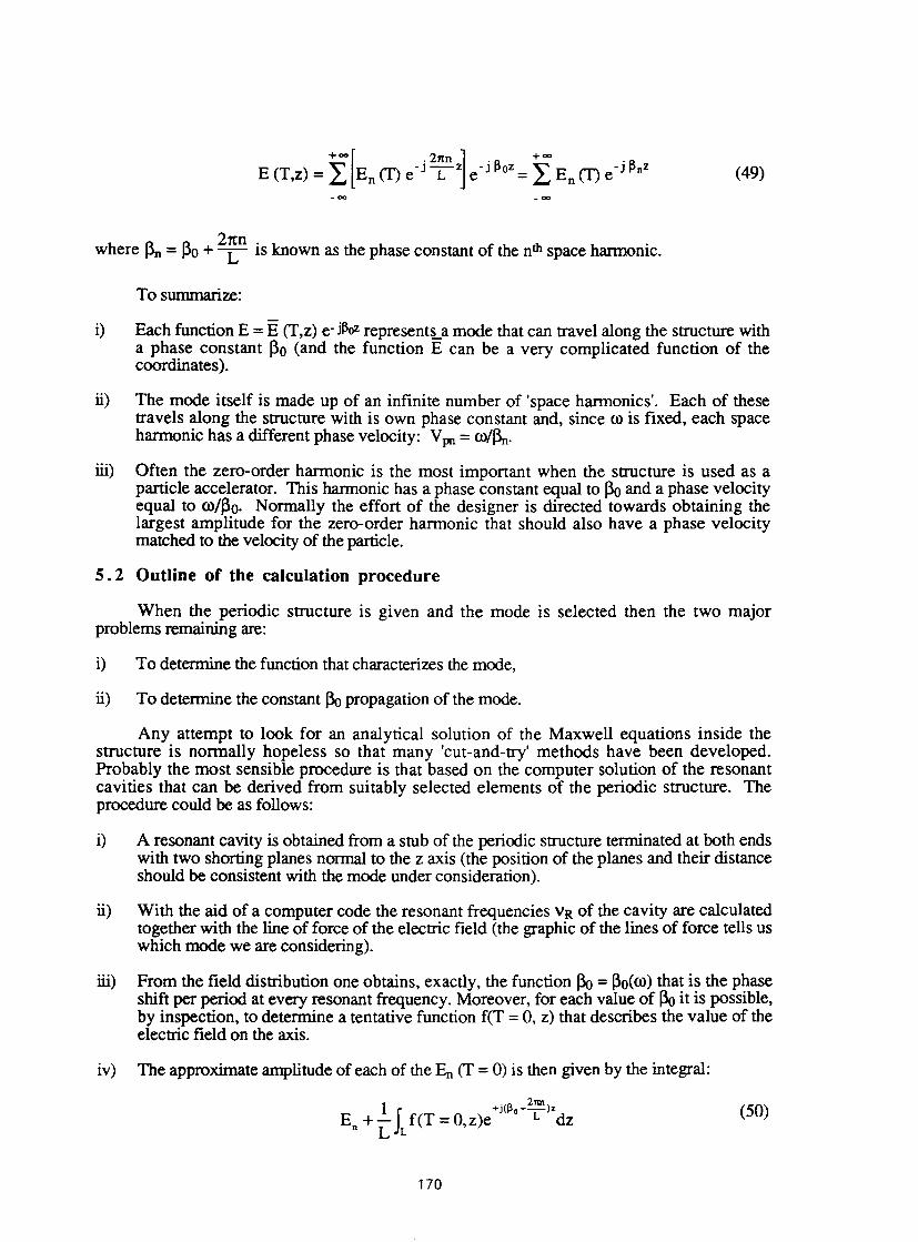
(49)

where ~ = ~o + 2~n is known as the phase constant of the nth space harmonic.

To summarire:

i) Each function E = E (T,z) e· j~oz represent~a mode that can travel along the structure with a phase constant ~o (and the function E can be a very complicated function of the coordinates).

ii) The mode itself is made up of an infinite number of 'space harmonics'. Each of these travels along the structure with is own phase constant and, since ro is fixed, each space harmonic has a different phase velocity: V pn = ro/~.

iii) Often the zero-order harmonic is the most important when the structure is used as a particle accelerator. This harmonic has a phase constant equal to ~o and a phase velocity equal to ro/~o. Normally the effort of the designer is directed towards obtaining the largest amplitude for the zero-order harmonic that should also have a phase velocity matched to the velocity of the particle.

5. 2 Outline of the calculation procedure

When the periodic structure is given and the mode is selected then the two major problems remaining are:

i) To determine the function that characterires the mode,

ii) To determine the constant J3<> propagation of the mode.

Any attempt to look for an analytical solution of the Maxwell equations inside the structure is normally hopeless so that many 'cut-and-try' methods have been developed. Probably the most sensible procedure is that based on the computer solution of the resonant cavities that can be derived from suitably selected elements of the periodic structure. The procedure could be as follows:

i)

ii)

iii)

iv)

A resonant cavity is obtained from a stub of the periodic structure terminated at both ends with two shorting planes normal to the z axis (the position of the planes and their distance should be consistent with the mode under consideration).

With the aid of a computer code the resonant frequencies VR of the cavity are calculated together with the line of force of the electric field (the graphic of the lines of force tells us which mode we are considering).

From the field distribution one obtains, exactly, the function J3<> = ~o(ro) that is the phase shift per period at every resonant frequency. Moreover, for each value of J3<> it is possible, by inspection, to determine a tentative function f(T = 0, z) that describes the value of the electric field on the axis.

The approximate amplitude of each of the En (T = 0) is then given by the integral:

1 + j(~o + 2itn )z

E +- r f(T = O,z)e L dz n Lh

(50)

170

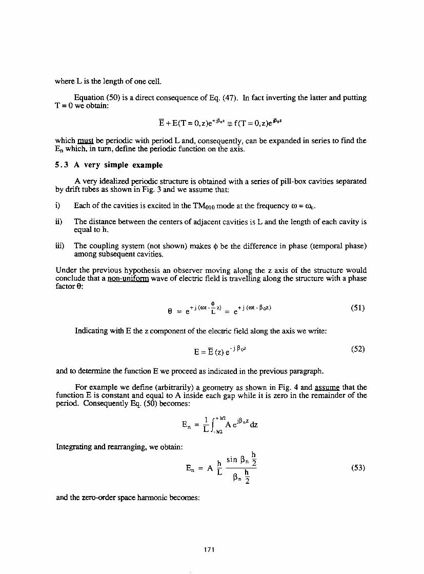
where L is the length of one cell.

Equation (50) is a direct consequence of Eq. (47). In fact inverting the latter and putting T = 0 we obtain:

E + E(T = O,z)e+illoz := f(T = O,z)eilloz

which .lllllS1 be periodic with period Land, consequently, can be expanded in series to find the En which, in turn, define the periodic function on the axis.

5. 3 A very simple example

A very idealized periodic structure is obtained with a series of pill-box cavities separated by drift tubes as shown in Fig. 3 and we assume that:

i) Each of the cavities is excited in the TMo10 mode at the frequency ro = COc.

ii) The distance between the centers of adjacent cavities is L and the length of each cavity is equal to h.

iii) The coupling system (not shown) makes<!> be the difference in phase (temporal phase) among subsequent cavities.

Under the previous hypothesis an observer moving along the z axis of the structure would conclude that a non-uniform wave of electric field is travelling along the structure with a phase factor 0:

+ j (cot - ~oz) e

Indicating with E the z component of the electric field along the axis we write:

and to determine the function E we proceed as indicated in the previous paragraph.

(51)

(52)

For example we define (arbitrarily) a geometry as shown in Fig. 4 and assume that the function Eis constant and equal to A inside each gap while it is zero in the remainder of the period. Consequently Eq. (50) becomes:

E = _!_ J + lv'2 A ej~nz dz n L -W2

Integrating and rearranging, we obtain:

and the zero-order space harmonic becomes:

171

(53)

. ii\ h h sm"'2L .~ h .~

E 0 = A - --- e-J-Lz= AL 't0

e-JLz

where 'to is transit time factor.

L cp~ 2L

I I

--~---------------------~-· I I

I hfl ,,,,,.U2_

I

z

Fig. 4 Assumed amplitude of the E field along the axis

It is interesting to note that:

(54)

i) A charged particle travelling along the z ax.is with real speed equal to roJJ3o would be synchronous with the zero-order space harmonic. If this particle is at the center of a gap when the field is maximum then the particle gains a voltage equal to Ah 'to for each period of the structure.

ii) The same result is obtained if one calculates the voltage gained by a charged particle that travels along the gap of a cavity with speed VP= roJ(cp/L) and passes through the center of the gap when the field is maximum.

iii) When a charged particle travels along a periodic structure, it experiences the effect of all the space harmonics. If the particle is synchronous with one space harmonic then only this harmonic continuously increases (or decreases) the energy of the particles. The other space hannonics are seen as alternating fields whose average effect is zero.

5. 4 An equivalent scheme for the corrugated waveguide and the Brillouin diagram

As already said a corrugated waveguide can be obtained by coupling a series of identical pill-box cavities through a central hole. In this way the coupling between two adjacent cavities is mainly capacitive. Consequently, an equivalent scheme that can represent the behaviour of the corrugated guide (in the fundamental mode) is given in Fig. 5. In this very elementary scheme the elements L and C represent the behaviour of the cavities while the capacitances k

172

represent the coupling among the cavities. It should be noticed that if the radius of coupling hole tends to zero then the cavities become 'uncoupled' and consequently the capacitances k should tend to infinity.

k k k k

L L L

Fig. 5 Simple equivalent scheme for a corrugated waveguide

To solve the network we write down the mesh equation for the nth cell:

In-1 ( 2 1 . L ) I In+ 1 0 - jrok + jrok + jroC + J ro n - jrok =

Now the Floquet theorem allows us to write:

In-1 = In e-j<!> ; In+l = In e+j<I>

if <I> = 0 is the reference phase for the nth cell. Substituting and solving we obtain:

where eor2 = 1/LC is the unperturbed radian resonant frequency of the cavities.

From the above solution we can draw the following conclusion:

(55)

i) The propagation is possible only inside the range of frequencies for which -1 <cos<!> <1. Consequently COr ::;; ro ::;; COr '11 +4 k/C and the structure exhibits only one pass band.

ii) Inside the pass band the frequency is an even function of the propagation constant <j>.

iii) If Lis the distance between the centers of two adjacent cavities, the phase constant ~ and the phase velocity VP of the voltage wave are respectively: ~ = <!>IL ; V p = roL/<j>.

It is rather obvious that an equivalent circuit cannot tell us the 'whole story' and many other important aspects of the theory should be examined using different schemes.

We should reconsider the propagation constants of the space harmonics. Let us rewrite the general expression for one component of the fields that travels along the periodic structure:

where 130 = 13o(ro) is the phase constant of the space harmonic of order zero. For the reasons already seen ro must be an even function of <I> = j30L inside the interval -1t < <I> < 7t. Now the

173

first order (forward) space harmonic has a phase constant ~1 = l3o + 21t/L. Consequently, if at some frequency the phase shift for the zero order space harmonic is 'I', then at the same frequency the phase shift for the first order space harmonic must be '1'+27t. The general conclusion is that inside the pass band of each mode the frequency is a periodic, even function of the phase constant with period equal to 21t/L.

The above considerations are summarized in the co-~ diagram which, for the fundamental mode of a corrugated waveguide appears as indicated in Fig. 6. We see that ro is a periodic even function of the phase constant. For ~ = 0 and ~ = 7t/L the tangents to the diagram are horizontal because at the corresponding frequencies the structure resonates and the group velocities go to zero. The tangents of the angles P and G respectively indicate the phase and group velocities of a field that travels with a phase shift <I> = 1C/2 per cell.

w

, -'ll"/L l+1t/L

I I '21'71.. I ?.T/\..

-ZERO OllOE.R :.w.c£ MA~NC»llC --+--FIRST OR.DER ~PACE WAnMONll.4

Fig. 6 Brillouin diagram for the fundamental mode of a corrugated waveguide

S. S Numerical example

We will now examine a procedure to determine the dispersion diagram for a mode that propagates along a periodic structure. We focus our attention on the structure most commonly used in the electron (positron) linear accelerators, the corrugated waveguide whose section is given in Fig. 7.

Corrugated guides are used to accelerate charged particles whose velocity is very near to the speed of light in vacuo. Consequently, we look for a TM mode, possibly without circumferential variations, that should have a phase velocity less than c. The cut-off of the TMo1 mode of the unperturbed guide is:

Ve= poi = 2.873 109 Hz 27t ..../ Eo µo a

174

! .. 25 .. ,

Fig. 7 Typical corrugated waveguide. All the dimensions are in mm.

while for the corrugated guide we find Ve= 2.928 GHz. This is due to the finite (and large) thickness of the washers. At this frequency the phase shift per cell is equal to zero and the corresponding phase velocity is infinite. Increasing the excitation frequency, the phase shift per cell becomes finite and at the end of the first stop band is equal to 7t.

At the frequency v1t for which ~ = 7t/L the phase velocity becomes V p1t = ©rr/(7t/L). The first design of the structure should be chosen in such a way as to render V p1t « c. Consequently one should expect that for a frequency v, between Ve and Vm the condinon Vp = c should be met. Once (as in our case) the structure is given, then to determine the first branch of the dispersion diagram and the frequency for which v2 = c, we find via the computer, the resonant frequencies of a series of cavities which include a ilifferent number of corrugations as shown in Fig. 8. Each cavity is obtained by short circuiting an element of the corrugated guide with two conducting planes which leaves a 'half cell' at both ends. In this way, to each resonant frequency corresponds a standing wave that can be interpreted as the result of two waves that travel in opposite directions along the axis. The modulus of the resulting field must be maximum on the shorting planes and this allows us to detennine the propagation constant of the two travelling waves that create the standing field (for clarity, each drawing contains the diagram of the values of the electric field on the axis). The couples ro,~ can be indicated as dots on a diagram. If the number of the dots is large enough, then the dispersion diagram can be interpolated. For the indicated structure the phase velocity equal to c is obtained for v - 2.947 GHz.

The density of resonances increases at both ends of the pass-band. For this reason designers prefer structures for which the wanted phase velocity is obtained when ~L = 7t/2 (the so-called 7r/2 mode operation). In this situation the E-field in the central cell is very small so that the stored energy is proportionally much smaller. This is the main reason that led to the invention of the so-called 'side-coupled corrugated guide', one in which the 'central cell' is located outside the main guide (D.T. Tran, private communication).

175

,~ L

--1 , .. 2l

--1 Ez N Ez I

z L _____ z I I I

I I

a) j3L = 1t ; flt = 2.965 GHz 1t b) j3L = 2 ; f1t/2 = 2.947 GHz

1· 3L

.. I 1· 3L

i Ez Ez

z --------- z

1t c) j3L = 3 ; f1t/3 = 2.938 GHz 2

d) j3L = 3 7t; fz131t = 2.957 GHz

Fig. 8 Sketches of the lines of force for four cases of the same pass-band

176

6. TECHNICAL APPROACH TO CAVITY DESIGN

6. 1 The reentrant cavity - physical picture

Consider two equal washers, made from a perfectly conducting material, axially separated by a small distanced, as shown in Fig. 9 a-b. If the separation dis much smaller than the radius Tl and the hole has a negligible area then the two washers create a capacitor that, in air or vacuum, has a capacity C === £o m 12/d. If this capacitor is charged then it is well-known that the lines of force of the electric field are nearly uniform at the inside and spread outside to have zero intensity at infinity.

--@

Fig. 9 Section and perspective view of the two washers

Now we connect the two washers with one loop of perfect conductor as indicated in Fig. 10 and it is clear that we have made a parallel resonating circuit with resonant frequency

f1 === 1 I (27t../LC.) if Lis the inductance of the loop. This resonant circuit 'radiates' energy with an efficiency that depends upon the resonant wavelength and the mechanical sizes of the circuit. Consequently we note that, due to the radiation, the oscillations will be damped. (This explains why the formula for fl cannot be exact.)

--© Fig. 10 Section and perspective view of the two washers connected with a loop

As a next step we add a second loop, equal and opposite to the first one. If we ignore the small coupling between the two loops we can then conclude that, because the capacity is nearly unchanged and the total inductance is just halved, the resonant frequency f 2 of the new device becomes:

(56)

177

If we try to increase the number of loops then we encounter some conceptual complications. Consider Fig. 11 where eight equal loops now connect the washers. We cannot expect that the actual resonant frequency f8 would be near to twice f 2 because with this geometry we should take into account the mutual couplings, at least between neighbouring loops. In general we see that the more we increase the number of loops the more the inductance of a single loop increases (the wire becomes thinner) as well as the mutual coupling between adjacent loops. So we have two processes in competition:

i) Increasing the number of loops in parallel tends to reduce the total inductance.

ii) Increasing the number of loops tends to increase the inductance of each loop together with their mutual coupling.

Fig. 11

0

Front and perspective view of the device with eight loops (for clarity four loops are omitted in the latter)

The more we increase the number of loops the larger is the modification of the shape of the magnetic field created by a single loop, as shown in Fig. 12 a-b.

0 a)

0 b)

Fig. 12 Section normal to the axis in two different situations: a) loops well separated, b) loops very close to each other

178

Evidently, when the loops are very close to each other the magnetic lines of force strongly interact, trying to enhance the field inside and to cancel the field between the wires. In the limit of an infinitely large number of loops we can conclude that: i) In the process of increasing the number of loops the oscillating (resonant) frequency of

the device increases but a limit should be expected.

ii) The electromagnetic field remains confined inside the dielectric volume limited by the perfectly conducting walls.

iii) Due to the confinement, the device cannot radiate and, as a consequence, any oscillations are undamped.

To summarize, when the number of loops tends to infinity we have a resonant cavity with at least one definite mode of oscillation. In this scheme, the so-called LC mode, the electrical energy initially stored inside the capacitor is converted, without losses, into magnetic energy inside the toroidal part of the cavity. This energy is then converted back to electrical energy and so on.

In the next paragraphs we will see many attempts to find, analytically, the resonant frequency for some cavities. This is done only to give a better understanding of the physics of the cavities rather than to obtain numerical results. When reliable numbers are required, the use of a computer code is strongly recommended even if, in a few cases, the analytical procedures can be used to give an idea of the mechanical sizes of the device.

6. 2 First approximation for the resonant frequency of the 'LC' model

We have seen that our device becomes a closed, toroidal, structure when the number of loops becomes infinite. The dielectric volume of this structure can be broadly split into the two parts, E and H, as shown in Fig. 13. The volume between the two disks contains the largest part of the electrical energy and for this reason is indicated at the E part of the cavity. The remaining volume contains the largest part of the magnetic field generated by the currents that flow over the inner surface of the conducting walls and for this reason is indicated as the H part of the cavity. Important also, the H part can also be seen as a 'magnetic circuit'.

Fig. 13 Views of the toroidal volume of the cavity

In Fig. 14 is sketched the axial cross section of a cavity very similar to the one already seen except that, in this case, the loops are placed only on one side of the capacitor.

179

r

t--~~~~~----.----------

dA dr

~""'7.:111,,,.,,.,.~~""" : : r!(: -r

-t--r 1

-------------- ---

.,... ___ k----t~

r 2 -r 1 ==k-d

- --------------•z

Fig. 14 Cross section of the 'LC' cavity with the gap on one side

We consider the magnetic circuit defined by the cylindrical sleeves of radii ri and r2 limited by the two circular crowns separated by the distance k. The currents injected onto the inner walls by the capacitor create a flux f whose lines of force are circular and are centered on the axis of the cavity. If the cross section of the toroid is approximately square and if we suppose that the magnetic field obeys the Biot-Savart law then the flux that passes through the cross section dA of a cylindrical crown with thickness equal to dr is:

I d<j>(r) = µ 0H(r)dA = µ 0-k dr

21tr

where I is the peak of the alternating current due to the capacitor.

The total flux is obtained by integrating Eq. (57). Taking into account that:

L = <l>/i = Equivalent inductance for one loop

we obtain:

(57)

(58)

If C = EQ7tr12/d is the capacity due to the central disk we obtain for the resonant frequency:

180

(59)

It should be emphasized that the heuristic procedure already outlined cannot give a very good approximation unless special geometrical conditions are realized. In fact:

i) The fringing field around the capacitor has been ignored but the contribution of this field to the total capacity may be large.

ii) The magnetic field in the cross section is a function both of r and z. Consequently the use of the Biot-Savart law may result in a very naive approximation.

iii) It is immediately seen, from the Maxwell equation, that the magnetic field cannot be zero inside the capacitive region. Similarly, the electric field cannot be zero inside the inductive, or H, region.

At this point the temptation to go through the many semi-theoretical artifices that until about 20 years ago were used for improving the accuracy of the formula should be rejected. Now, in fact, powerful computer programs exist that can easily calculate the resonant frequency of a cylindrical cavity with an accuracy better than 10-4. Consequently, analytical methods are no longer used for this purpose.

It seems important to point out some consequences of Eq. (59):

i) In passing from a finite number of loops to a 'closed volume' the resonating frequency tends to a finite value fo.

ii) The electromagnetic field in the cavity can oscillate sinusoidally with frequency fo and maintains a fixed shape. In other words the field is standing and is monochromatic.

iii) Since the geometrical shape of the loops has not been specified, it follows that the previous procedures are applicable to cavities of different shape as shown, for example, in Fig. 15.

1) 2) 3) 4)

Fig. 15 Four different cross sections of fundamentally similar cavities. In spite of their similarity they are given different names: 1 and 2) nose-cone cavities, 3 and 4) disk­loaded cavities

181

The above heuristic treatment should have shown that a cavity resonator is basically a device with distributed inductance and capacitance. Consequently, we conclude that the behaviour of a resonant cavity can be solved by using the Maxwell equation inside the volume of the cavity, as will be seen later on.

Figure 16 shows three examples of LC cavities together with the lines of force of the electric fields and the value of the resonant frequencies. (The sizes of typical cavities are r2 = 0.40 m, ri = 0.10 m, k = 0.3 m. The gaps are 0.01, 0.02 and 0.06 for a), b) and c) respectively.)

The analytic formula* (59) gives a good result for the a) cavity while the approximation is very poor for the cavity c). This should have been expected since in the latter case the electrical energy stored in the gap volume no longer dominates the total electrical energy stored in the cavity.

--------...... -·

-·-·--·- -·-·-- -·---

a) b) c)

vo = 84.2 MHz (104) vo = 107.8 MHz (148) vo = 153.3 MHz (256)

Fig. 16 Three different profiles of an LC cavity (the cavities are symmetric and only half the section is shown). vo is the resonant frequency from a computer program while the value in parenthesis comes from the analytical formula.

6. 3 The coaxial cavity

A very important class of cavity resonators are defined by the relation l > d > r1 - r1. In this case the cavity is made from a piece of coaxial cable short-circuited at one end and capacitively loaded at the other as sketched in Fig. 17. For these cavities the previous approximation no longer holds mainly because the fundamental resonant wavelength becomes 'comparable' with the geometrical length of the cavity. Consequently, the magnetic field between the cylindrical walls cannot be uniform along the axis as was assumed for the previous LC cavity.

* The resonant cavities have many different uses and the dielectric volume can be made from many different dielectrics. In the case of the accelerating cavities, the dielectric is vacuum or part air and part vacuum. In order to avoid confusion from now on, we will assume that the dielectric is isotropic with permittivity £ and permeability µ.

182

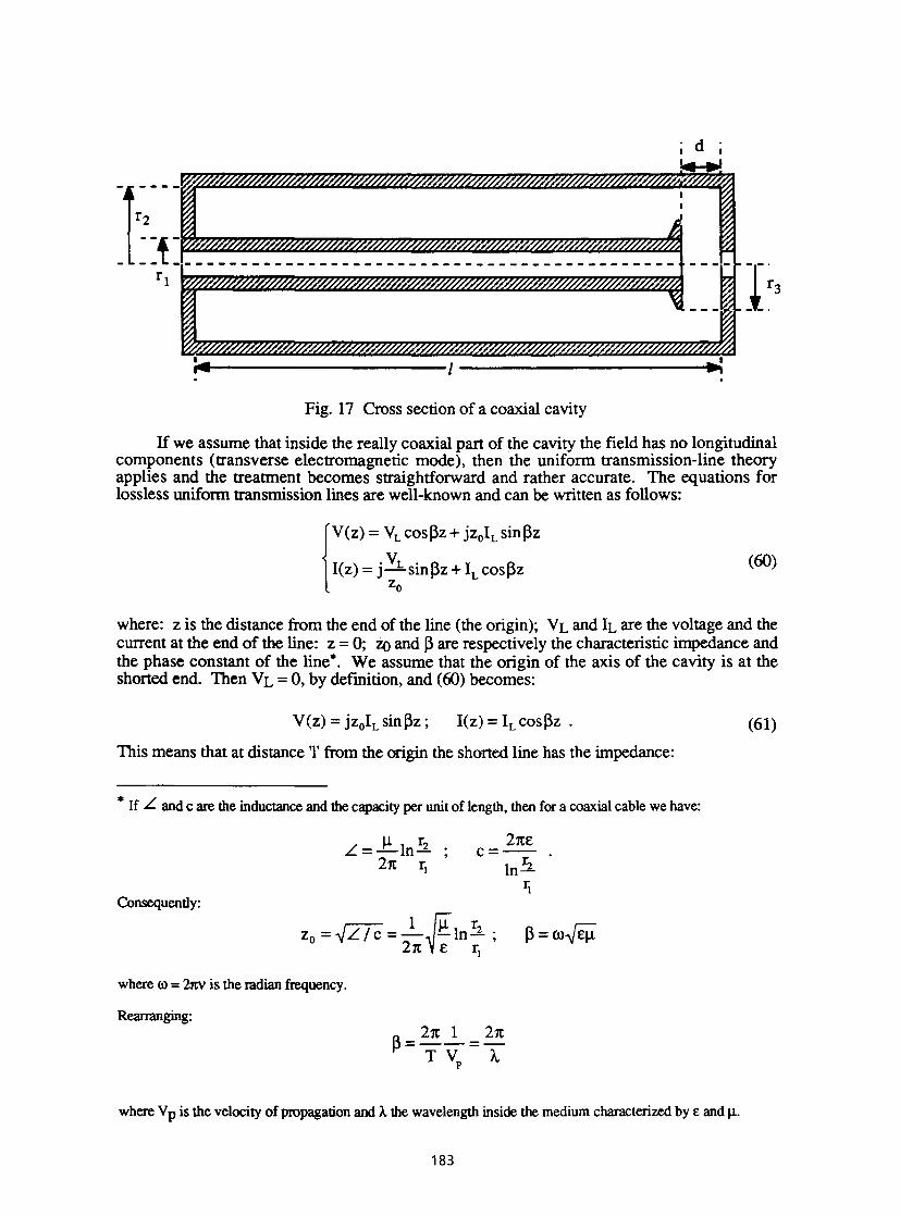
Fig. 17 Cross section of a coaxial cavity

If we assume that inside the really coaxial part of the cavity the field has no longitudinal components (transverse electromagnetic mode), then the uniform transmission-line theory applies and the treatment becomes straightforward and rather accurate. The equations for lossless uniform transmission lines are well-known and can be written as follows:

{

V(z) = VL cosj3z + jz0IL sinj3z

l(z) = j VL sinj3z +IL cosj3z Zo

(60)

where: z is the distance from the end of the line (the origin); VL and IL are the voltage and the current at the end of the line: z = 0; zo and 13 are respectively the characteristic impedance and the phase constant of the line*. We assume that the origin of the axis of the cavity is at the shorted end. Then VL = 0, by definition, and (60) becomes:

I(z) =IL cosj3z .

This means that at distance 'l' from the origin the shorted line has the impedance:

* If L and c are the inductance and the capacity per unit of length, then for a coaxial cable we have:

Consequently:

21tE c=--

z0 = .../ L I c = -1- /µIn r2 ;

21t y; r1

1 r1 n-1i

where ro = 2xv is the radian frequency.

Rearranging: A- 21t 1 _ 21t p-----

T VP A

where V p is the velocity of propagation and A. the wavelength inside the medium characterized by £ and µ.

183

(61)

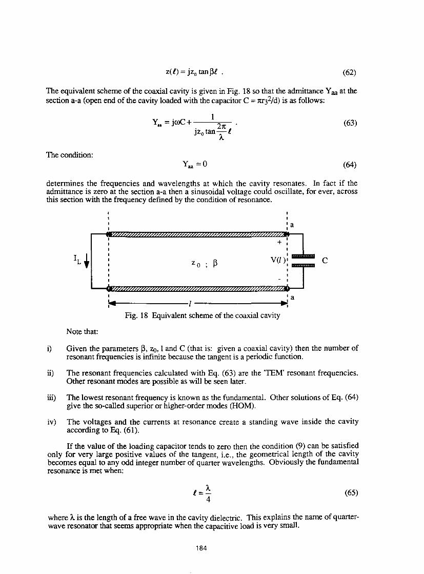
z(l) = jz0 tan Pl . (62)

The equivalent scheme of the coaxial cavity is given in Fig. 18 so that the admittance Y aa at the section a-a (open end of the cavity loaded with the capacitor C = m32/d) is as follows:

1 Y .. = jroC+ 2 . 1tl

JZ0 tanT (63)

The condition: (64)

determines the frequencies and wavelengths at which the cavity resonates. In fact if the admittance is zero at the section a-a then a sinusoidal voltage could oscillate, for ever, across this section with the frequency defined by the condition of resonance.

IL t

Note that:

I I

•a I

IP

+ I

I

Zo p V(/ )• I

- I

•a ~:4---~~~~~~~-1~~~~~~~~~-..~·

Fig. 18 Equivalent scheme of the coaxial cavity

c

i) Given the parameters p, zo, 1 and C (that is: given a coaxial cavity) then the number of resonant frequencies is infinite because the tangent is a periodic function.

ii) The resonant frequencies calculated with Eq. (63) are the 'TEM' resonant frequencies. Other resonant modes are possible as will be seen later.

iii) The lowest resonant frequency is known as the fundamental. Other solutions of Eq. (64) give the so-called superior or higher-order modes (HOM).

iv) The voltages and the currents at resonance create a standing wave inside the cavity according to Eq. (61).

If the value of the loading capacitor tends to zero then the condition (9) can be satisfied only for very large positive values of the tangent, i.e., the geometrical length of the cavity becomes equal to any odd integer number of quarter wavelengths. Obviously the fundamental resonance is met when:

A. l=-

4 (65)

where A. is the length of a free wave in the cavity dielectric. This explains the name of quarter­wave resonator that seems appropriate when the capacitive load is very small.

184

When the capacitive load is large the geometrical length of the cavity becomes much shorter than A./4 and the name of foreshortened coaxial cavity is more appropriate even though both are used indifferently. The larger the characteristic impedance of the coaxial cable is the larger is the sensitivity of the resonant frequency to the loading capacity.

If the resonant frequency Vo = roo/2rc of the cavity is known then the distribution of the voltage and of the current can be calculated. Let V(l) =Vo be the gap voltage at resonance. Then from the first expression of Eq. (61) we obtain the amplitude of the current IL on the shorted end (z = 0):

I . V0 _.V0~1 L=-J =+J- + . z0 sin j3.t z0 tan 2 j3.t

(66)

Introducing the value of tan f31 obtained from (63) and (64) we obtain:

IL =+j Vo ~l+(ro0Cz0 )2. Zo

Substituting this value in (61) the required current and voltage distributions are found and we conclude:

i) The amplitude of the current is maximum at the short and its value is always larger than Vo/zo.

ii) The current lags the voltage by rc/2 and a purely standing wave is set up.

iii) The voltage and current have sinusoidal distribution.

iv) At the open end the current is equal to roo C Vo and this current accounts for the 'shortening' of the cavity with respect to A./4.

Before ending this section we note that a coaxial cavity can be used in two different ways a) and b) as shown in Fig. 19. In a) the beam transits one gap and it is well-known that for each particle the net energy gain depends upon many factors (gap voltage, phase of the particle, transit time, etc.). In b) the beam transits two gaps in series, where the E fields are always at 180. to each other. Consequently the effect of one gap can cumulate with the effect of the other if and only if the distance L between the mid-planes of the two gaps obeys the synchronism law that the transit time over the distance L should be equal to half of the period T of the RF voltage.

V· T V ·TC A. L=-=- -=J3-

2 c 2 2 (67)

where J3 is the relative velocity of the particle and A, is the free space wavelength of the accelerating field. It is unfortunate that the phase constant of a transmission system and the relative velocity of the particle have the same symbol.

The reader may wonder why a coaxial resonator is not always used in the 'b' mode since the effect of one resonator can be doubled. The answer is very complex and demands a careful analysis of the accelerator in which the coaxial cavity should be used. Broadly it can be said that optimization between voltage on one side and mechanical size and complication on the other is the most important element for the final choice.

185

a) b)

Fig. 19 Two ways of using the coaxial cavity. The dashed lines indicate the beam axis.

6. 4 The A./2 cavity

The ')J2 cavity is realized with a stub or coaxial cable loaded with two equal capacitors kt at each end and with another capacitor k1 placed at the middle of the structure as shown in Fig. 20.

- - -~=2:2:2:2:2:2:2:2:2:2:2:2:2:2:2:2:2:2:2~- - -

~ - - · Beam axis

k1

L=2/

W/&'$###4 l?ff$##'M,,0J

l I 1· kt

I I ;zo;~

I k1 I ;zo;~

I ki

@0000'/#'t0i1 W#'#'h&ff4l a

Fig. 20 Simplified axial section and equivalent scheme of the /.J2 cavity

186

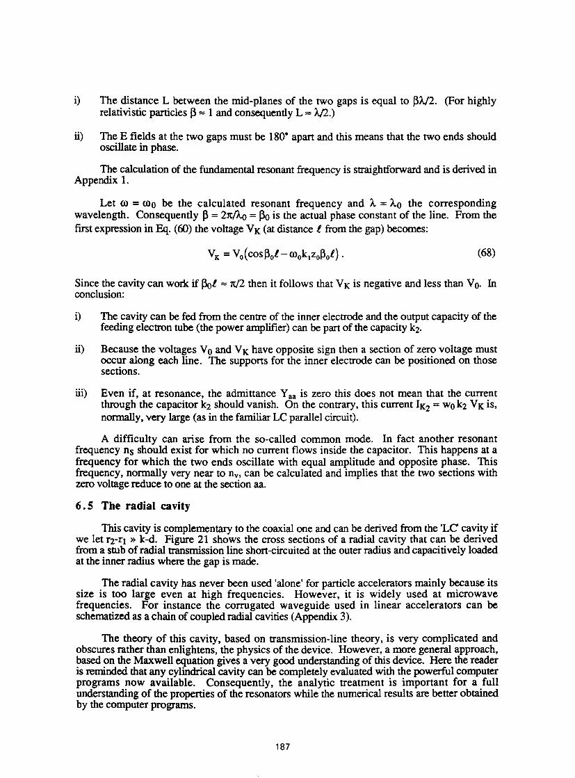
i) The distance L between the mid-planes of the two gaps is equal to ~A./2. (For highly relativistic particles~= 1 and consequently L = A./2.)

ii) The E fields at the two gaps must be 1 so· apart and this means that the two ends should oscillate in phase.

The calculation of the fundamental resonant frequency is straightforward and is derived in Appendix 1.

Let co = coo be the calculated resonant frequency and A. = A.o the corresponding wavelength. Consequently ~ = 2x/Ao = ~ is the actual phase constant of the line. From the first expression in Eq. (60) the voltage VK (at distance l from the gap) becomes:

(68)

Since the cavity can work if ~l = x/2 then it follows that V K is negative and less than Vo. In conclusion:

i) The cavity can be fed from the centre of the inner electrode and the output capacity of the feeding electron tube (the power amplifier) can be part of the capacity k1.

ii) Because the voltages V 0 and V K have opposite sign then a section of zero voltage must occur along each line. The supports for the inner electrode can be positioned on those sections.

iii) Even if, at resonance, the admittance Y aa is zero this does not mean that the current through the capacitor k1 should vanish. On the contrary, this current IK2 = wok2 VK is, normally, very large (as in the familiar LC parallel circuit).

A difficulty can arise from the so-called common mode. In fact another resonant frequency ns should exist for which no current flows inside the capacitor. This happens at a frequency for which the two ends oscillate with equal amplitude and opposite phase. This frequency, normally very near to nv. can be calculated and implies that the two sections with zero voltage reduce to one at the section aa.

6. S The radial cavity

This cavity is complementary to the coaxial one and can be derived from the 'LC' cavity if we let r1-r1 » k-d. Figure 21 shows the cross sections of a radial cavity that can be derived from a stub of radial transmission line short-circuited at the outer radius and capacitively loaded at the inner radius where the gap is made.

The radial cavity has never been used 'alone' for particle accelerators mainly because its size is too large even at high frequencies. However, it is widely used at microwave frequencies. For instance the corrugated waveguide used in linear accelerators can be schematized as a chain of coupled radial cavities (Appendix 3).

The theory of this cavity, based on transmission-line theory, is very complicated and obscures rather than enlightens, the physics of the device. However, a more general approach, based on the Maxwell equation gives a very good understanding of this device. Here the reader is reminded that any cylindrical cavity can be completely evaluated with the powerful computer programs now available. Consequently, the analytic treatment is important for a full understanding of the properties of the resonators while the numerical results are better obtained by the computer programs.

187

Fig. 21 Cross sections of a radial cavity

6. 7 Technical remarks

Now we consider a physical cavity, i.e., one that could be installed in an accelerator. It differs from the corresponding ideal cavity for at least the following reasons:

i) The walls have a finite conductivity so the currents that flow there cause energy dissipation.

ii) The cavity must be connected to the power amplifier, to the tuner, and to the sensors for the feedbacks, the monitors and meters. Each of these devices requires the creation of a hole and the use of non-perfect dielectric which introduces energy dissipation.

iii) The internal surfaces of the cavity (metallic and dielectric) at the microscopic level are highly complex and irregular from the chemical, physical and mechanical point of view. This promotes local electrical micro-discharges and heating. The consequent power dissipation may induce localized avalanche and or thermionic discharge with severe effects on the behaviour of the cavity.

iv) Poor vacuum is responsible for 'dark' and or luminescent discharges which in turn introduce erratic and unpredictable loads.

v) Electrons inside the evacuated part of the cavity are accelerated by the existing field and in colliding with the cavity walls extract new electrons. If the extraction efficiency is larger than one and the transit time between two impacts is very near to a half period of the accelerating voltage then a large cloud of electrons is built up that severely loads the cavity (the multipacting phenomenon).

188

Even if all the previous effects can be minimized or even prevented we can easily conclude that some power will be spent in supporting the required E field inside the cavity. In the large majority of cases (ignoring the ferrite-loaded cavities) this power loss depends upon the Joule effect on the walls.

In general a physical cavity should be considered as derived from an ideal one, the lossless model, through a series of small perturbations (holes ... electrodes ... dielectrics). Consequently, the modes of the model and the corresponding ones of the physical cavity should have, practically, the same form.

To evaluate the Joule losses we assume that:

i) The working mode of the physical cavity and the value of the electric field required at a convenient point are given.

ii) The quality factor of the considered mode is, a priori, very large.

If the above hypotheses are verified then we can assume that the working mode of the physical cavity almost coincides with the corresponding one of the model. Also, the amplitude of the magnetic field H is known everywhere inside the cavity and, in particular, on the walls where the H field is assumed to be purely tangential: H = Ht. (This is, in fact, the consequence of our approximation because the lossless model demands ideal walls where, on the other hand, the magnetic field cannot have the normal component.)

Since on a perfectly conducting wall the amplitude j of the linear density current must be equal to the amplitude of the magnetic field j = n x Ht then the power lost on the walls in maintaining the required level of excitation is obtained by integration on the surface S of the cavity:

(69)

where Rs is the surface resistivity of the walls (Appendix 2).

Evidently the value of the power consumption depends upon the level of excitation of the cavity. On the other hand when the excitation at one point is given (for the selected mode) the excitation level is defined for the whole volume of the cavity. The transient behaviour of a cavity depends upon the energy storage of the cavity which is directly proportional to the quality factor Q. Consequently in designing a cavity remember that:

i) The gap voltage and the aperture required are the relevant parameters for defining the geometry of the gap.

ii) The available volume and its geometrical shape together with the required resonant frequency determine the choice of the kind of cavity and of its operating mode.

iii) The final mechanical sizes depend upon the requirements laid on the quality factor and on the parallel shunt resistance.

iv) Experience suggests that, as a rule, the cavity should be designed to work in the fundamental rather than higher-order mode.

189

7 . EXCITATION AND TUNING OF A CAVITY

Power is brought to the cavity with a waveguide, a coaxial cable or by direct connection to a power amplifier. In bringing the power from the power supply (the final amplifier) to the cavity two conditions should be fulfilled:

i) The transmission system must not radiate.

ii) The cavity should be matched to the transmission system.

The first condition is satisfied by the use of coaxial cables and waveguides which barely radiate. The second depends upon the device that 'couples' the cavity to the line. Very many solutions are possible and these can be grouped as described in the following sections.

7 .1 Magnetic coupling (Fig. 22)

Here electrical power excites a loop that is coupled to the cavity. This means that the magnetic field created by the loop should have a component in common with the magnetic field of the mode we wish to excite in the cavity. As shown in Fig. 22 the loops are placed in the region of the cavity where the magnetic field is stronger.

Fig. 22 Two examples of loop coupling

7. 2 Electric coupling (Fig. 23)

In this case a capacitive coupling is created by placing the exciting electrode where the electric field is stronger. This coupling is simple and efficient but is inherently connected with the creation of high gradients that must be carefully evaluated to avoid the risk of dark and or glow discharges.

7. 3 Direct coupling (Fig. 24)

In this case the transmission system should be connected directly to the 'hot' electrode of the cavity. This may be convenient if, avoiding the transmission line, the plate or the cathode of the final tube can be directly connected with the hot electrode of the cavity. This solution is particularly useful when the electrode connected with the plate is DC-isolated from the remainder of the cavity (for instance as in the Segal cavity sketched on the left side of the figure). In most cases this does not happen and a decoupling capacitor is normally used. Obviously other solutions are possible such as feeding the tube via the cathode with a negative voltage and allowing the potential of the shell of the cavity to float

190

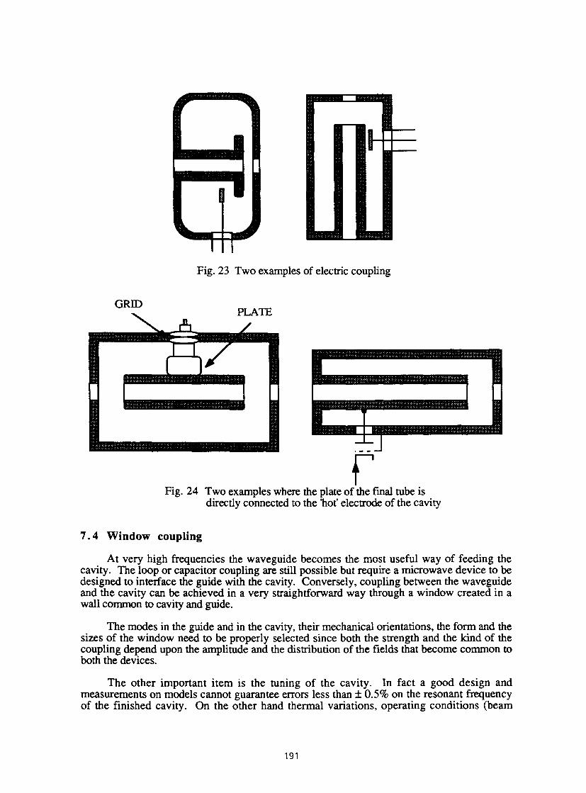
Fig. 23 Two examples of electric coupling

GRID PLAIB

r Fig. 24 Two examples where the plate of the final tube is

directly connected to the 'hot' electrode of the cavity

7. 4 Window coupling

At very high frequencies the waveguide becomes the most useful way of feeding the cavity. The loop or capacitor coupling are still possible but require a microwave device to be designed to interface the guide with the cavity. Conversely, coupling between the waveguide and the cavity can be achieved in a very straightforward way through a window created in a wall common to cavity and guide.

The modes in the guide and in the cavity, their mechanical orientations, the form and the sizes of the window need to be properly selected since both the strength and the kind of the coupling depend upon the amplitude and the distribution of the fields that become common to both the devices.

The other important item is the tuning of the cavity. In fact a good design and measurements on models cannot guarantee errors less than± 0.5% on the resonant frequency of the finished cavity. On the other hand thermal variations, operating conditions (beam

191

loading) and changes required in the coupling with the power amplifier require that a continuous tuning of the cavity should be always possible.

As a rule any change in the shape of the cavity may introduce a shift in the resonant frequency and consequently could be used for tuning the cavity. In general movable pistons or paddles are introduced into the cavity to vary the stored magnetic or electrical energy with consequent variation of the frequency. These devices introduce losses and, in general, tuning ranges between two and three per cent are the most that one can hope for. Variation of the position of the short circuit at the end of the coaxial cavities is very effective if applicable.

Sometimes axial squeezing of the cavity has been used. This method has the advantage of perturbing the electrical behaviour of the cavity but requires a precise, powerful, mechanical device. Moreover the axial compression and extension should be so small as to avoid mechanical fatigue failure of the material, the creating of microcracks in the welds or damage to the vacuum joints.

Remembering that heat due to electrical losses introduces small changes in the mechanical size of the cavity, fine tuning can be achieved by simply controlling the local temperature of the cooling fluid.

ACKNOWLEDGEMENT

My thanks are due to Ms. Marina Nadalin for typing the manuscript, and to Dr. Cristina Pasotti for the numerical computations.

* * * BIBLIOGRAPHY

1) R.E. Collin, Field Theory of Guided Waves, McGraw Hill, New York (1961).

2) C.G. Montgomery, R.H. Dike and E.M. Purcell, Principles of Microwave Circuits, M.I.T. Radiation Lab. Series, Mc Graw Hill, (1948).

3) T. Moreno, Microwave Transmission Design Data, Dover Pub. Inc., (1958).

4) J.C. Slater, Microwave Electronics, Dover Pub. Inc., (1969).

5) S. Ramo, J.R. Whinnery and T. van Duzer, Fields and Waves in Communication Electronics, John Wiley & Sons, (1984).

6) E.T. Whittaker and G.N. Watson, A Course of Modem Analysis, 4th ed., Cambridge Univ. Press, Cambridge, England, (1952).

192

APPENDIX 1

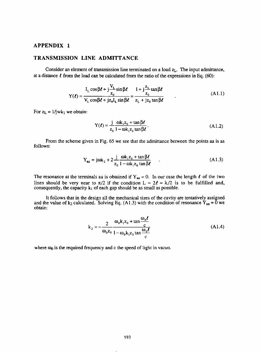
TRANSMISSION LINE ADMITTANCE

Consider an element of transmission line terminated on a load ZL. The input admittance, at a distance l from the load can be calculated from the ratio of the expressions in Eq. (60):

For ZL = l/jwk1 we obtain:

Y(l) = j rok1z0 + tanj3.l . z0 1 - rok1 z0 tan j3.l

(Al.1)

(Al.2)

From the scheme given in Fig. 65 we see that the admittance between the points aa is as follows:

Y _ . k

2 j rok1z0 + tanJ3l

aa - J(J) 2 + z0 1 - rok1 z0 tan J3l

(Al.3)

The resonance at the terminals aa is obtained if Y aa = 0. In our case the length l of the two lines should be very near to x/2 if the condition L = 2l ""' /.../2 is to be fulfilled and, consequently, the capacity k1 of each gap should be as small as possible.

It follows that in the design all the mechanical sizes of the cavity are tentatively assigned and the value of k2 calculated. Solving Eq. (Al.3) with the condition of resonance Yaa = 0 we obtain:

(J) (I) l oZo 1-ro k z tan-0-o I 0

c

where COo is the required frequency and c the speed of light in vacuo.

193

(Al.4)

APPENDIX 2

EQUIVALENT RESISTANCE OF A CAVITY SURFACE

With reference to a left handed cartesian system of axes x, y, z, let the plane z = 0 be the boundary between two regions. Region (1), for which z is negative, is filled with a perfect dielectric while region (2) is filled with a material with conductivity equal to a. Suppose that on the plane z = 0 there is an electric field E such that:

where i is the versor of the x axis, Eo is a constant and ro = 2nv is the radian frequency of the field.

The Maxwell equations, written for the fields in the region (2) are as follows:

V x '.E = -jroµl{ ; V x H = cr'.E + jroc.E ; V • '.E = V • H = O

and from the first curl equation we obtain:

H -H- 1 aEx Y - -- jroµ Tz (A2.1)

Making the curl of the first equation and substituting the V x H from the second we obtain:

V x V x '.E = -jroµ[ cr'.E + jcoc'.E] . (A2.2)

Taking into account that V x V x A = V V •A - V'2 A and the condition on the divergence Eq. (A2.l) becomes:

V' 2'.E + ro 2Eµ - jroµcr'.E = 0 . (A2.3)

Since we assumed that E has only the x component we can put E = Ex = Ethen (A2.3) can be rewritten in a more tractable form:

d2E 2 ( • a) -+ro Eµ 1-J- E=O

dz2 roe (A2.4)

Integrating we obtain:

where (A2.5)

From (A2.1) we obtain:

E E2 H = - 1 e-YL - - e+'YZ zo zo

where - \} jroµ zo - cr+jroE

194

is the characteristic impedance of the medium.

Since for z = oo the fields should remain finite, the integration constant E2 should be zero and we obtain:

f E (z) = E0 e -YL

\

Eo -YL H (z) =- e ·

Zo (A2.6)

Now we remember that the normal radio-frequency technique does not consider wavelengths shorter than 0.1 mm and that at those extremely high frequencies the dimensionless quantity a/roE is larger than 105 even for very poor conductors such as lead.

Consequently neglecting one over 105 in the (A2.4), we obtain:

E =E0 exp(-fii -./roµ <> z) = E0 exp[- (l+j) ~] (A2.7)

where 8 = 1/--J 1tVµa is called the penetration, or the skin depth, constant.

The infinitesimal current that flows through any cross section (normal to the x axis) with unitary width and height equal to dz is:

ell =aE(z) dz .

Integrating between z = 0 and oo we obtain the total current that flows across any section of the conducting medium that has unitarian width and infinite length:

I= E a8 0 1 + i

(Note that I has the dimension of amperes/meter; the same as for a magnetic field.)

(A2.8)

The ratio Zs between the already defined current and the value of the surface field that causes the current is called the surface impedance of the conductor.

z = Eo = 1 + j = R (1 + J.) [Q] s I a8 s

(A2.9)

where R5 = 1/00 is the surface resistance of the material at the considered frequency.

We conclude that:

i) The electromagnetic field penetrates inside the conducting medium but undergoes a strong attenuation. In fact for frequencies above 1 MHz the penetration depth is less than 7•1 Q-5 meters for copper.

ii) The surface impedance offered by the conducting surface is complex with an angle of 45° electrical.

195

that the total current I flows in a slab of the same prism that has height equal to o. It follows that we can assume that any element of the conducting surface offers an equivalent resistance Req:

R = _!_ Length = 1 Length = R Length . eq CJ o • Width Ocr Width s Width

(A2.10)

Equation (A2.10) can be extended for evaluating the equivalent resistance of any element of surface by taking the infinitesimal length and width parallel and normal to the line of the current respectively. (In this general case these elements are both functions of the coordinates.) Once the equivalent resistance of an element of surface is defined then the formula can be immediately derived. For example, for a tubular element with constant cross section (A2.10) can be rewritten:

R =Rs Length eq Perimeter

(A2.ll)

The surface resistance Rs is defined for smooth surfaces. In other words the microscopic irregularities of the surface must be much smaller than the penetration depth. If this is not so, the lengths and widths must be evaluated taking into account the irregularities. The conductivity, penetration depth and surface resistance for the more common conductors are given below:

Silver Copper Aluminium

CJ

6.17 x 107 5.80 x 107 3.72 x 107

0 0.066/-../v 0.060/-.Jv 0.082/-.Jv

where CJ is in Mhos/meter, O is in meters and Rs in ohms.

196

Rs 2.53 x 10-7-.Jv 2.61 x 10-7-.Jv 3.28 x 10-7-.Jv

APPENDIX 3

RADIAL CAVITY AND RELATED ACCELERATING STRUCTURES

We consider the radial cavity (normally known as the pill-box cavity) sketched in Fig. 25 and referred to cylindrical coordinates. In this particular (but important) exercise we assume that the electric field Eis parallel to z and depends only upon the radius and the time. Due to these hypotheses the general equation (7) reduces to the familiar Bessel equation of zero order:

(A3.l)

for which the general solution is:

(A3.2)

where: Jo and No are (respectively) the Bessel and the Newman function of zero order while A, B and L are the integration constants and the eigenvalues to be determined.

I

I I

--'-

z

Fig. 25 The pill-box cavity

Because the volume of the cavity includes a portion of the z axis then B should be equal to zero. Moreover the condition n x E = 0 on the wall is automatically satisfied for z = 0 and z = h. Conversely, because Eis parallel to zit follows that the above condition can be met if, and only if, the vector E is equal to zero for r = a and just this condition determines the eigenvalue. In fact the condition Jo(A) = 0 means that we should have:

At= Pot l = 1,2,3,... (A3.3) a

where Pol is the 'l' zero of the Bessel function of zero order. If the permittivity and permeability of the dielectric that fills the cavity are Eo and µo respectively, the resonant frequencies of the cavity (for the described mode) are:

A p Vt= t = 0.477 108 ......Qf.Hz . (A3.4)

2rt~E0µ0 a

For l = 1 (Pol = 2.405) we obtain the lowest resonant frequency to which corresponds the wavelength A= 2.61 a.

197