Rin Vout Rin + Rf Rf Rin
789
100 Solutions Manual 6th Edition Feedback Control of Dynamic Systems . . Gene F. Franklin . J. David Powell . Abbas Emami-Naeini . . . . Assisted by: H.K. Aghajan H. Al-Rahmani P. Coulot P. Dankoski S. Everett R. Fuller T. Iwata V. Jones F. Safai L. Kobayashi H-T. Lee E. Thuriyasena M. Matsuoka
-
Upload
independent -
Category
Documents
-
view
0 -
download
0
Transcript of Rin Vout Rin + Rf Rf Rin

100
Solutions Manual6th Edition
Feedback Control of DynamicSystems
.
.
Gene F. Franklin.
J. David Powell.
Abbas Emami-Naeini.
.
.
.
Assisted by:H.K. AghajanH. Al-RahmaniP. CoulotP. DankoskiS. EverettR. FullerT. IwataV. JonesF. Safai
L. KobayashiH-T. Lee
E. ThuriyasenaM. Matsuoka
CD1
Stamp

Chapter 1
An Overview and BriefHistory of Feedback Control
1.1 Problems and Solutions
1. Draw a component block diagram for each of the following feedback controlsystems.
(a) The manual steering system of an automobile
(b) Drebbel�s incubator
(c) The water level controlled by a �oat and valve
(d) Watt�s steam engine with �y-ball governor
In each case, indicate the location of the elements listed below andgive the units associated with each signal.
� the process� the process output signal� the sensor� the actuator� the actuator output signal� The reference signal
Notice that in a number of cases the same physical device may per-form more than one of these functions.
Solution:
(a) A manual steering system for an automobile:
101

102CHAPTER 1. AN OVERVIEWAND BRIEF HISTORYOF FEEDBACK CONTROL
(b) Drebbel�s incubator:
(c) Water level regulator:
(d) Fly-ball governor:

1.1. PROBLEMS AND SOLUTIONS 103
(e) Automatic steering of a ship:
(f) A public address system:
2. Identify the physical principles and describe the operation of the thermo-stat in your home or o¢ ce.
Solution:
A thermostat is a device for maintaining a temperature constant at adesired value. It is equipped with a temperature sensor which detectsdeviation from the desired value, determines whether the temperaturesetting is exceeded or not, and transmits the information to a furnaceor air conditioner so that the termperature in the room is brought back

104CHAPTER 1. AN OVERVIEWAND BRIEF HISTORYOF FEEDBACK CONTROL
T h i c ks t o c k
C o n s i s t e n c ym e t e r
C o n t r o l l e rW h i t ew a t e r
C V
R e f i n e rM a c h i n ec h e s t
S t o r a g ec h e s t
W i r e
M o i s t u r em e t e r
S c r e e n sa n d c l e a n e r s
H e a d b o x D r y i n gs e c t i o n
P r e s s e s R e e l
Figure 1.1: A paper making machine From Karl Astrom, (1970, page 192)reprinted with permission.
to the desired setting. Examples: Tubes �lled with liquid mercuryare attached to a bimetallic strip which tilt the tube and cause the mer-cury to slide over electrical contacts. A bimetallic strip consists of twostrips of metal bonded together, each of a di¤erent expansion coe¢ cientso that temperature changes bend the metal. In some cases, the bendingof bimetallic strips simply cause electrical contacts to open or close di-rectly. In most cases today, temperature is sensed electronically using,forexample, a thermistor, a resistor whose resistance changes with tempera-ture. Modern computer-based thermostats are programmable, sense thecurrent from the thermistor and convert that to a digital signal.
3. A machine for making paper is diagrammed in Fig. 1.12. There are twomain parameters under feedback control: the density of �bers as controlledby the consistency of the thick stock that �ows from the headbox onto thewire, and the moisture content of the �nal product that comes out of thedryers. Stock from the machine chest is diluted by white water returningfrom under the wire as controlled by a control valve (CV). A meter suppliesa reading of the consistency. At the �dry end�of the machine, there is amoisture sensor. Draw a signal graph and identify the seven componentslisted in Problem 1 for
(a) control of consistency
(b) control of moisture
Solution:
(a) Control of paper machine consistency:

1.1. PROBLEMS AND SOLUTIONS 105
(b) Control of paper machine moisture:
4. Many variables in the human body are under feedback control. For eachof the following controlled variables, draw a graph showing the processbeing controlled, the sensor that measures the variable, the actuator thatcauses it to increase and/or decrease, the information path that completesthe feedback path, and the disturbances that upset the variable. You mayneed to consult an encyclopedia or textbook on human physiology forinformation on this problem.
(a) blood pressure
(b) blood sugar concentration
(c) heart rate
(d) eye-pointing angle
(e) eye-pupil diameter
Solution:
Feedback control in human body:

106CHAPTER 1. AN OVERVIEWAND BRIEF HISTORYOF FEEDBACK CONTROL
Variable Sensor Actuator Information path Disturbancesa) Blood pressure -Arterial -Cardiac output -A¤erent nerve -Bleeding
baroreceptors -Arteriolar/venous �bers -Drugsdilation -Stress,Pain
b) Blood sugar -Pancreas -Pancreas secreting -Blood �ow to -Dietconcentration insulin pancreas -Exercise(Glucose)c) Heart rate -Diastolic volume -Electrical stimulation -Mechanical draw -Hormone release
sensors of sino-atrial node of blood from heart -Exercise-Cardiac sympathetic and cardiac muscle -Circulatingnerves epinephrine
d) Eye pointing -Optic nerve -Extraocular muscles -Cranial innervation -Head movementangle -Image detection -Muscle twitche) Pupil diameter -Rods -Pupillary sphincter -Autonomous -Ambient light
muscles system -Drugsf ) Blood calcium -Parathyroid gland -Ca from bones to blood - Parathormone -Ca need in boneslevel detectors -Gastrointestinal hormone a¤ecting -Drugs
absorption e¤ector sites
5. Draw a graph of the components for temperature control in a refrigeratoror automobile air-conditioning system.
Solution:
This is the simplest possible system. Modern cases include computercontrol as described in later chapters.
6. Draw a graph of the components for an elevator-position control. Indi-cate how you would measure the position of the elevator car. Consider acombined coarse and �ne measurement system. What accuracies do yousuggest for each sensor? Your system should be able to correct for thefact that in elevators for tall buildings there is signi�cant cable stretch asa function of cab load.
Solution:
A coarse measurement can be obtained by an electroswitch located beforethe desired �oor level. When touched, the controller reduces the motorspeed. A ��ne� sensor can then be used to bring the elevator preciselyto the �oor level. With a sensor such as the one depicted in the �gure,a linear control loop can be created (as opposed to the on-o¤ type of thecoarse control).Accuracy required for the course switch is around 5 cm;for the �ne �oor alignment, an accuracy of about 2 mm is desirable toeliminate any noticeable step for those entering or exiting the elevator.

1.1. PROBLEMS AND SOLUTIONS 107
7. Feedback control requires being able to sense the variable being controlled.Because electrical signals can be transmitted, ampli�ed, and processedeasily, often we want to have a sensor whose output is a voltage or currentproportional to the variable being measured. Describe a sensor that wouldgive an electrical output proportional to:
(a) temperature(b) pressure(c) liquid level(d) �ow of liquid along a pipe (or blood along an artery) force(e) linear position(f) rotational position(g) linear velocity(h) rotational speed(i) translational acceleration(j) torque
Solution:Sensors for feedback control systems with electrical output. Exam-ples
(a) Temperature: Thermistor- temperature sensitive resistor with resis-tance change proportional to temperature; Thermocouple; Thyrister.Modern thermostats are computer controlled and programmable.
(b) Pressure: Strain sensitive resistor mounted on a diaphragm whichbends due to changing pressure

108CHAPTER 1. AN OVERVIEWAND BRIEF HISTORYOF FEEDBACK CONTROL
(c) Liquid level: Float connected to potentiometer. If liquid is conductivethe impedance change of a rod immersed in the liquid may indicatethe liquid level.
(d) Flow of liquid along a pipe: A turbine actuated by the �ow with amagnet to trigger an external counting circuit. Hall e¤ect producesan electronic output in response to magnetic �eld changes. Anotherway: Measure pressure di¤erence from venturi into pressure sensoras in �gure; Flowmeter. For blood �ow, an ultrasound device like aSONAR can be used.
(e) Position.When direct mechanical interaction is possible and for �small�dis-placements, the same ideas may be used. For example a potentiome-ter may be used to measure position of a mass in an accelerator (h).However in many cases such as the position of an aircraft, the task ismuch more complicated and measurement cannot be made directly.Calculation must be carried out based on other measurements, forexample optical or electromagnetic direction measurements to severalknown references (stars,transmitting antennas ...); LVDT for linear,RVDT for rotational.
(f) Rotational position. The most common traditional device is a pote-niometer. Also common are magnetic machines in shich a rotatingmagnet produces a variable output based on its angle.
(g) Linear velocity. For a vehicle, a RADAR can measure linear velocity.In other cases, a rack-and-pinion can be used to translate linear torotational motion and an electric motor(tachometer) used to measurethe speed.
(h) Speed: Any toothed wheel or gear on a rotating part may be used totrigger a magnetic �eld change which can be used to trigger an elec-trical counting circuit by use of a Hall e¤ect (magnetic to electrical)sensor. The pulses can then be counted over a set time interval toproduce angular velocity: Rate gyro; Tachometer

1.1. PROBLEMS AND SOLUTIONS 109
(i) Acceleration: A mass movement restrained by a spring measured bya potentiometer. A piezoelectric material may be used instead (a ma-terial that produces electrical current with intensity proportional toacceleration). In modern airbags, an integrated circuit chip containsa tiny lever and �proof mass�whose motion is measured generating avoltage proportional to acceleration.
(j) Force, torque: A dynamometer based on spring or beam de�ections,which may be measured by a potentiometer or a strain-gauge.
8. Each of the variables listed in Problem 7 can be brought under feedbackcontrol. Describe an actuator that could accept an electrical input and beused to control the variables listed. Give the units of the actuator outputsignal.
Solution:
(a) Resistor with voltage applied to it ormercury arc lamp to generateheat for small devices. a furnace for a building..
(b) Pump: Pumping air in or out of a chamberto generate pressure. Else,a �torque motor�produces force..
(c) Valve and pump: forcing liquid in or out of the container.
(d) A valve is nromally used to control �ow.
(e) Electric motor
(f) Electric motor
(g) Electric motor
(h) Electric motor
(i) Translational acceleration is usually controlled by a motor or engineto provide force on the vehicle or other object.
(j) Torque motor. In this motor the torque is directly proportional tothe input (current).

Chapter 2
Dynamic Models
Problems and Solutions for Section 2.1
1. Write the di¤erential equations for the mechanical systems shown in Fig. 2.39.For (a) and (b), state whether you think the system will eventually de-cay so that it has no motion at all, given that there are non-zero initialconditions for both masses, and give a reason for your answer.
Figure 2.39: Mechanical systems
Solution:
2003

2004 CHAPTER 2. DYNAMIC MODELS
The key is to draw the Free Body Diagram (FBD) in order to keep thesigns right. For (a), to identify the direction of the spring forces on theobject, let x2 = 0 and �xed and increase x1 from 0. Then the k1 springwill be stretched producing its spring force to the left and the k2 springwill be compressed producing its spring force to the left also. You can usethe same technique on the damper forces and the other mass.
(a)Free body diagram for Problem 2.1(a)
m1�x1 = �k1x1 � b1 _x1 � k2 (x1 � x2)m2�x2 = �k2 (x2 � x1)� k3 (x2 � y)� b2 _x2
There is friction a¤ecting the motion of both masses; therefore thesystem will decay to zero motion for both masses.
Free body diagram for Problem 2.1(b)
m1�x1 = �k1x1 � k2(x1 � x2)� b1 _x1m2�x2 = �k2(x2 � x1)� k3x2
Although friction only a¤ects the motion of the left mass directly,continuing motion of the right mass will excite the left mass, andthat interaction will continue until all motion damps out.

2005
Figure 2.40: Mechanical system for Problem 2.2
m1 m2
x1 x2
k (x x )2 1 2 k (x x )2 1 2
k x1 1
b (x x )1 1 2 b (x x )1 1 2. .. .
F
Free body diagram for Problem 2.1(c)
m1�x1 = �k1x1 � k2(x1 � x2)� b1( _x1 � _x2)
m2�x2 = F � k2(x2 � x1)� b1( _x2 � _x1)
2. Write the di¤erential equations for the mechanical systems shown in Fig. 2.40.State whether you think the system will eventually decay so that it hasno motion at all, given that there are non-zero initial conditions for bothmasses, and give a reason for your answer.
Solution:
The key is to draw the Free Body Diagram (FBD) in order to keep thesigns right. To identify the direction of the spring forces on the left sideobject, let x2 = 0 and increase x1 from 0. Then the k1 spring on the leftwill be stretched producing its spring force to the left and the k2 springwill be compressed producing its spring force to the left also. You can usethe same technique on the damper forces and the other mass.
m1 m2
x1 x2
x2
k (x x )2 1 2
k x1 1 k1
b (x x )2 1 2 b (x x )2 1 2. . . .
Free body diagram for Problem 2.2

2006 CHAPTER 2. DYNAMIC MODELS
Then the forces are summed on each mass, resulting in
m1�x1 = �k1x1 � k2(x1 � x2)� b1( _x1 � _x2)
m2�x2 = k2(x1 � x2)� b1( _x1 � _x2)� k1x2
The relative motion between x1 and x2 will decay to zero due to thedamper. However, the two masses will continue oscillating togetherwithout decay since there is no friction opposing that motion and no �ex-ure of the end springs is all that is required to maintain the oscillation ofthe two masses.
3. Write the equations of motion for the double-pendulum system shown inFig. 2.41. Assume the displacement angles of the pendulums are smallenough to ensure that the spring is always horizontal. The pendulumrods are taken to be massless, of length l, and the springs are attached3/4 of the way down.
Figure 2.41: Double pendulum
Solution:

2007
1θ 2θ
k
1sin43 θl 2sin
43 θl
m m
l43
De�ne coordinates
If we write the moment equilibrium about the pivot point of the left pen-dulem from the free body diagram,
M = �mgl sin �1 � k3
4l (sin �1 � sin �2) cos �1
3
4l = ml2��1
ml2��1 +mgl sin �1 +9
16kl2 cos �1 (sin �1 � sin �2) = 0
Similary we can write the equation of motion for the right pendulem
�mgl sin �2 + k3
4l (sin �1 � sin �2) cos �2
3
4l = ml2��2
As we assumed the angles are small, we can approximate using sin �1 ��1; sin �2 � �2, cos �1 � 1, and cos �2 � 1. Finally the linearized equationsof motion becomes,
ml��1 +mg�1 +9
16kl (�1 � �2) = 0
ml��2 +mg�2 +9
16kl (�2 � �1) = 0
Or

2008 CHAPTER 2. DYNAMIC MODELS
��1 +g
l�1 +
9
16
k
m(�1 � �2) = 0
��2 +g
l�2 +
9
16
k
m(�2 � �1) = 0
4. Write the equations of motion of a pendulum consisting of a thin, 4-kgstick of length l suspended from a pivot. How long should the rod be inorder for the period to be exactly 2 secs? (The inertia I of a thin stickabout an endpoint is 1
3ml2. Assume � is small enough that sin � �= �.)
Solution:
Let�s use Eq. (2.14)
M = I�;
mg
θ
2lO
De�ne coordinatesand forces
Moment about point O.
MO = �mg � l
2sin � = IO��
=1
3ml2��
�� +3g
2lsin � = 0

2009
As we assumed � is small,
�� +3g
2l� = 0
The frequency only depends on the length of the rod
!2 =3g
2l
T =2�
!= 2�
s2l
3g= 2
l =3g
2�2= 1:49m
<Notes>
(a) Compare the formula for the period, T = 2�q
2l3g with the well known
formula for the period of a point mass hanging with a string with
length l. T = 2�q
lg .
(b) Important!In general, Eq. (2.14) is valid only when the reference point forthe moment and the moment of inertia is the mass center of thebody. However, we also can use the formular with a reference pointother than mass center when the point of reference is �xed or notaccelerating, as was the case here for point O.
5. For the car suspension discussed in Example 2.2, plot the position ofthe car and the wheel after the car hits a �unit bump� (i.e., r is a unitstep) using MATLAB. Assume that m1 = 10 kg, m2 = 350 kg, kw =500; 000 N=m, ks = 10; 000 N=m. Find the value of b that you wouldprefer if you were a passenger in the car.
Solution:
The transfer function of the suspension was given in the example in Eq.(2.12) to be:
(a)
Y (s)
R(s)=
kwbm1m2
(s+ ksb )
s4 + ( bm1+ b
m2)s3 + ( ksm1
+ ksm2+ kw
m1)s2 + ( kwb
m1m2)s+ kwks
m1m2
:
This transfer function can be put directly into Matlab along withthe numerical values as shown below. Note that b is not the damping

2010 CHAPTER 2. DYNAMIC MODELS
ratio, but damping. We need to �nd the proper order of magnitudefor b, which can be done by trial and error. What passengers feelis the position of the car. Some general requirements for the smoothride will be, slow response with small overshoot and oscillation.
From the �gures, b � 3000 would be acceptable. There is too muchovershoot for lower values, and the system gets too fast (and harsh)for larger values.
% Problem 2.5clear all, close all
m1 = 10;m2 = 350;kw = 500000;ks = 10000;B = [ 1000 2000 3000 4000 ];t = 0:0.01:2;
for i = 1:4b = B(i);num = kw*b/(m1*m2)*[1 ks/b];den =[1 (b/m1+b/m2) (ks/m1+ks/m2+kw/m1)
(kw*b/(m1*m2) kw*ks/(m1*m2)];sys=tf(num,den);y = step( sys, t );
subplot(2,2,i);plot( t, y(:,1), �:�, t, y(:,2), �-�);legend(�Wheel�,�Car�);ttl = sprintf(�Response with b = %4.1f �,b );title(ttl);
end
6. Write the equations of motion for a body of mass M suspended from a�xed point by a spring with a constant k. Carefully de�ne where thebody�s displacement is zero.
Solution:
Some care needs to be taken when the spring is suspended vertically inthe presence of the gravity. We de�ne x = 0 to be when the spring isunstretched with no mass attached as in (a). The static situation in (b)results from a balance between the gravity force and the spring.

2011
From the free body diagram in (b), the dynamic equation results
m�x = �kx�mg:
We can manipulate the equation
m�x = �k�x+
m
kg�;
so if we replace x using y = x+ mk g,
m�y = �kym�y + ky = 0
The equilibrium value of x including the e¤ect of gravity is at x = �mk g
and y represents the motion of the mass about that equilibrium point.
An alternate solution method, which is applicable for any probleminvolving vertical spring motion, is to de�ne the motion to be with respectto the static equilibrium point of the springs including the e¤ect of gravity,and then to proceed as if no gravity was present. In this problem, wewould de�ne y to be the motion with respect to the equilibrium point,then the FBD in (c) would result directly in
m�y = �ky:
7. Automobile manufacturers are contemplating building active suspensionsystems. The simplest change is to make shock absorbers with a change-able damping, b(u1): It is also possible to make a device to be placed inparallel with the springs that has the ability to supply an equal force, u2;in opposite directions on the wheel axle and the car body.

2012 CHAPTER 2. DYNAMIC MODELS
(a) Modify the equations of motion in Example 2.2 to include such con-trol inputs.
(b) Is the resulting system linear?
(c) Is it possible to use the forcer, u2; to completely replace the springsand shock absorber? Is this a good idea?
Solution:
(a) The FBD shows the addition of the variable force, u2; and shows bas in the FBD of Fig. 2.5, however, here b is a function of the controlvariable, u1: The forces below are drawn in the direction that wouldresult from a positive displacement of x.
Free body diagram
m1�x = b (u1) ( _y � _x) + ks (y � x)� kw (x� r)� u2m2�y = �ks (y � x)� b (u1) ( _y � _x) + u2
(b) The system is linear with respect to u2 because it is additive. Butb is not constant so the system is non-linear with respect to u1 be-cause the control essentially multiplies a state element. So if we addcontrollable damping, the system becomes non-linear.
(c) It is technically possible. However, it would take very high forcesand thus a lot of power and is therefore not done. It is a much bet-ter solution to modulate the damping coe¢ cient by changing ori�cesizes in the shock absorber and/or by changing the spring forces byincreasing or decreasing the pressure in air springs. These featuresare now available on some cars... where the driver chooses betweena soft or sti¤ ride.
8. Modify the equation of motion for the cruise control in Example 2.1,Eq(2.4), so that it has a control law; that is, let u = K(vr � v); where
vr = reference speed
K = constant:

2013
This is a �proportional�control law where the di¤erence between vr andthe actual speed is used as a signal to speed the engine up or slow it down.Put the equations in the standard state-variable form with vr as the inputand v as the state. Assume that m = 1000 kg and b = 50 N � s=m; and�nd the response for a unit step in vr using MATLAB. Using trial anderror, �nd a value of K that you think would result in a control system inwhich the actual speed converges as quickly as possible to the referencespeed with no objectional behavior.
Solution:
_v +b
mv =
1
mu
substitute in u = K (vr � v)
_v +b
mv =
1
mu =
K
m(vr � v)
Rearranging, yields the closed-loop system equations,
_v +b
mv +
K
mv =
K
mvr
A block diagram of the scheme is shown below where the car dynamicsare depicted by its transfer function from Eq. 2.7.
mbs
m+
1KΣ
u vrv
−+
Block diagram
The transfer function of the closed-loop system is,
V (s)
Vr(s)=
Km
s+ bm +
Km
so that the inputs for Matlab are

2014 CHAPTER 2. DYNAMIC MODELS
num =K
m
den = [1b
m+K
m]
For K = 100; 500; 1000; 5000 We have,
Time (sec.)
Am
plitu
de
Step Response
0 5 10 15 20 25 30 35 400
0.1
0.2
0.3
0.4
0.5
0.6
0.7
0.8
0.9
1From: U(1)
To: Y
(1)
K=100
K=500
K=1000
K=5000
Time responses
We can see that the larger the K is, the better the performance, with noobjectionable behaviour for any of the cases. The fact that increasing Kalso results in the need for higher acceleration is less obvious from theplot but it will limit how fast K can be in the real situation because theengine has only so much poop. Note also that the error with this schemegets quite large with the lower values of K. You will �nd out how toeliminate this error in chapter 4 using integral control, which is containedin all cruise control systems in use today. For this problem, a reasonablecompromise between speed of response and steady state errors would beK = 1000; where it responds is 5 seconds and the steady state error is 5%.

2015
% Problem 2.8clear all, close all
% datam = 1000;b = 50;k = [ 100 500 1000 5000 ];
% Overlay the step responsehold onfor i=1:length(k)K=k(i);num =K/m;den = [1 b/m+K/m];step( num, den);
end
9. In many mechanical positioning systems there is �exibility between onepart of the system and another. An example is shown in Figure 2.6where there is �exibility of the solar panels. Figure 2.42 depicts such asituation, where a force u is applied to the mass M and another massm is connected to it. The coupling between the objects is often modeledby a spring constant k with a damping coe¢ cient b, although the actualsituation is usually much more complicated than this.
(a) Write the equations of motion governing this system.
(b) Find the transfer function between the control input, u; and theoutput, y:
Figure 2.42: Schematic of a system with �exibility
Solution:
(a) The FBD for the system is

2016 CHAPTER 2. DYNAMIC MODELS
Free body diagrams
which results in the equations
m�x = �k (x� y)� b ( _x� _y)
M �y = u+ k (x� y) + b ( _x� _y)
or
�x+k
mx+
b
m_x� k
my � b
m_y = 0
� k
Mx� b
M_x+ �y +
k
My +
b
M_y =
1
Mu
(b) If we make Laplace Transform of the equations of motion
s2X +k
mX +
b
msX � k
mY � b
msY = 0
� k
MX � b
MsX + s2Y +
k
MY +
b
MsY =
1
MU
In matrix form,�ms2 + bs+ k � (bs+ k)� (bs+ k) Ms2 + bs+ k
� �XY
�=
�0U
�From Cramer�s Rule,
Y =
det
�ms2 + bs+ k 0� (bs+ k) U
�det
�ms2 + bs+ k � (bs+ k)� (bs+ k) Ms2 + bs+ k
�=
ms2 + bs+ k
(ms2 + bs+ k) (Ms2 + bs+ k)� (bs+ k)2U
Finally,

2017
Y
U=
ms2 + bs+ k
(ms2 + bs+ k) (Ms2 + bs+ k)� (bs+ k)2
=ms2 + bs+ k
mMs4 + (m+M)bs3 + (M +m)ks2

2018 CHAPTER 2. DYNAMIC MODELS
Problems and Solutions for Section 2.2
10. A �rst step toward a realistic model of an op amp is given by the equationsbelow and shown in Fig. 2.43.
Vout =107
s+ 1[V+ � V�]
i+ = i� = 0
Figure 2.43: Circuit for Problem 10.
Find the transfer function of the simple ampli�cation circuit shown usingthis model.
Solution:
As i� = 0,
(a)Vin � V�Rin
=V� � Vout
Rf
V� =Rf
Rin +RfVin +
RinRin +Rf
Vout
Vout =107
s+ 1[V+ � V�]
=107
s+ 1
�V+ �
RfRin +Rf
Vin �Rin
Rin +RfVout
�= � 107
s+ 1
�Rf
Rin +RfVin +
RinRin +Rf
Vout
�

2019
Figure 2.44: Circuit for Problem 11.
VoutVin
=�107 Rf
Rin+Rf
s+ 1 + 107 Rin
Rin+Rf
11. Show that the op amp connection shown in Fig. 2.44 results in Vo = Vinif the op amp is ideal. Give the transfer function if the op amp has thenon-ideal transfer function of Problem 2.10.
Solution:
Ideal case:
Vin = V+
V+ = V�
V� = Vout
Non-ideal case:
Vin = V+; V� = Vout
but,
V+ 6= V�
instead,
Vout =107
s+ 1[V+ � V�]
=107
s+ 1[Vin � Vout]

2020 CHAPTER 2. DYNAMIC MODELS
so,
VoutVin
=107
s+1
1 + 107
s+1
=107
s+ 1 + 107�=
107
s+ 107
12. Show that, with the non-ideal transfer function of Problem 2.10, the opamp connection shown in Fig. 2.45 is unstable.
Figure 2.45: Circuit for Problem 12.
Solution:
Vin = V�; V+ = Vout
Vout =107
s+ 1[V+ � V�]
=107
s+ 1[Vout � Vin]
VoutVin
=107
s+1
107
s+1 � 1=
107
�s� 1 + 107�=
�107s� 107
The transfer function has a denominator with s� 107; and the minus signmeans the exponential time function is increasing, which means that ithas an unstable root.
13. A common connection for a motor power ampli�er is shown in Fig. 2.46.The idea is to have the motor current follow the input voltage and theconnection is called a current ampli�er. Assume that the sense resistor,Rs is very small compared with the feedback resistor, R and �nd thetransfer function from Vin to Ia: Also show the transfer function whenRf =1:

2021
Solution:
At node A,Vin � 0Rin
+Vout � 0Rf
+VB � 0R
= 0 (93)
At node B, with Rs � R
Ia +0� VBR
+0� VBRs
= 0 (94)
VB =RRsR+Rs
Ia
VB � RsIa
The dynamics of the motor is modeled with negligible inductance as
Jm��m + b _�m = KtIa (95)
Jms+ b = KtIa
At the output, from Eq. 94. Eq. 95 and the motor equation Va =IaRa +Kes
Vo = IaRs + Va
= IaRs + IaRa +KeKtIaJms+ b
Substituting this into Eq.93
VinRin
+1
Rf
�IaRs + IaRa +Ke
KtIaJms+ b
�+IaRsR
= 0
This expression shows that, in the steady state when s ! 0; the currentis proportional to the input voltage.
If fact, the current ampli�er normally has no feedback from the outputvoltage, in which case Rf !1 and we have simply
IaVin
= � R
RinRs
14. An op amp connection with feedback to both the negative and the positiveterminals is shown in Fig 2.47. If the op amp has the non-ideal transferfunction given in Problem 10, give the maximum value possible for thepositive feedback ratio, P =
r
r +Rin terms of the negative feedback
ratio,N =Rin
Rin +Rffor the circuit to remain stable.
Solution:

2022 CHAPTER 2. DYNAMIC MODELS
Figure 2.46: Op Amp circuit for Problem 14.
Vin � V�Rin
+Vout � V�
Rf= 0
Vout � V+R
+0� V+r
= 0
V� =Rf
Rin +RfVin +
RinRin +Rf
Vout
= (1�N)Vin +NVoutV+ =
r
r +RVout = PVout
Vout =107
s+ 1[V+ � V�]
=107
s+ 1[PVout � (1�N)Vin �NVout]
VoutVin
=
107
s+ 1(1�N)
107
s+ 1P � 107
s+ 1N � 1
=107 (1�N)
107P � 107N � (s+ 1)
=�107 (1�N)
s+ 1� 107P + 107N

2023
0 < 1� 107P + 107NP < N + 10�7
15. Write the dynamic equations and �nd the transfer functions for the circuitsshown in Fig. 2.48.
(a) passive lead circuit
(b) active lead circuit
(c) active lag circuit.
(d) passive notch circuit
Solution:
(a) Passive lead circuitWith the node at y+, summing currents into that node, we get
Vu � VyR1
+ Cd
dt(Vu � Vy)�
VyR2
= 0 (96)
rearranging a bit,
C _Vy +
�1
R1+1
R2
�Vy = C _Vu +
1
R1Vu
and, taking the Laplace Transform, we get
Vy(s)
Vu(s)=
Cs+ 1R1
Cs+�1R1+ 1
R2
�(b) Active lead circuit
inV outV
C
V
1R 2R
fR
Active lead circuit with node marked
Vin � VR2
+0� VR1
+ Cd
dt(0� V ) = 0 (97)

2024 CHAPTER 2. DYNAMIC MODELS
Vin � VR2
=0� VoutRf
(98)
We need to eliminate V . From Eq. 98,
V = Vin +R2RfVout
Substitute V �s in Eq. 97.
1
R2
�Vin � Vin �
R2RfVout
�� 1
R1
�Vin +
R2RfVout
��C
�_Vin +
R2Rf
_Vout
�= 0
1
R1Vin + C _Vin = �
1
Rf
��1 +
R2R1
�Vout +R2C _Vout
�Laplace Transform
VoutVin
=Cs+ 1
R1
� 1Rf
�R2Cs+ 1 +
R2
R1
�= �Rf
R2
s+ 1R1C
s+ 1R1C
+ 1R2C
We can see that the pole is at the left side of the zero, which meansa lead compensator.
(c) active lag circuit
inR
inV outV
1R2R
C
V
Active lag circuit with node marked
Vin � 0Rin
=0� VR2
=V � VoutR1
+ Cd
dt(V � Vout)
V = � R2Rin
Vin

2025
VinRin
=� R2
RinVin � VoutR1
+ Cd
dt
�� R2Rin
Vin � Vout�
=1
R1
�� R2Rin
Vin � Vout�+ C
�� R2Rin
_Vin � _Vout
�1
Rin
�1 +
R2R1
�Vin +
1
RinR2C _Vin = �
1
R1Vout � C _Vout
VoutVin
= � R1Rin
R2Cs+ 1 +R2
R1
R1Cs+ 1
= � R2Rin
s+ 1R2C
+ 1R1C
s+ 1R1C
We can see that the pole is at the right side of the zero, which meansa lag compensator.
(d) notch circuit
outV
C1VC
C2
R R2/R
+ +
− −
inV
2V
Passive notch �lter with nodes marked
Cd
dt(Vin � V1) +
0� V1R=2
+ Cd
dt(Vout � V1) = 0
Vin � V2R
+ 2Cd
dt(0� V2) +
Vout � V2R
= 0
Cd
dt(V1 � Vout) +
V2 � VoutR
= 0
We need to eliminat V1; V2 from three equations and �nd the relationbetween Vin and Vout
V1 =Cs
2�Cs+ 1
R
� (Vin + Vout)V2 =
1R
2�Cs+ 1
R
� (Vin + Vout)

2026 CHAPTER 2. DYNAMIC MODELS
CsV1 � CsVout +1
RV2 �
1
RVout
= CsCs
2�Cs+ 1
R
� (Vin + Vout) + 1
R
1R
2�Cs+ 1
R
� (Vin + Vout)� �Cs+ 1
R
�Vout
= 0
C2s2 + 1R2
2�Cs+ 1
R
�Vin =
"�Cs+
1
R
��C2s2 + 1
R2
2�Cs+ 1
R
�#VoutVoutVin
=
C2s2+ 1R2
2(Cs+ 1R )�
Cs+ 1R
�� C2s2+ 1
R2
2(Cs+ 1R )
=
�C2s2 + 1
R2
�2�Cs+ 1
R
�2 � �C2s2 + 1R2
�=
C2�s2 + 1
R2C2
�C2s2 + 4CsR + 1
R2
=s2 + 1
R2C2
s2 + 4RC s+
1R2C2
16. The very �exible circuit shown in Fig. 2.49 is called a biquad becauseits transfer function can be made to be the ratio of two second-order orquadratic polynomials. By selecting di¤erent values for Ra; Rb; Rc; andRd the circuit can realise a low-pass, band-pass, high-pass, or band-reject(notch) �lter.
(a) Show that if Ra = R; and Rb = Rc = Rd =1; the transfer functionfrom Vin to Vout can be written as the low-pass �lter
VoutVin
=A
s2
!2n+ 2�
s
!n+ 1
(99)
where
A =R
R1
!n =1
RC
� =R
2R2

2027
Figure 2.47: Op-amp biquad
(b) Using the MATLAB comand step compute and plot on the samegraph the step responses for the biquad of Fig. 2.43 for A = 1;!n = 1; and � = 0:1; 0:5; and 1:0:
Solution:
Before going in to the speci�c problem, let�s �nd the general form of thetransfer function for the circuit.
VinR1
+V3R
= ��V1R2
+ C _V1
�V1R
= �C _V2V3 = �V2
V3Ra
+V2Rb
+V1Rc
+VinRd
= �VoutR
There are a couple of methods to �nd the transfer function from Vin toVout with set of equations but for this problem, we will directly solve forthe values we want along with the Laplace Transform.
From the �rst three equations, slove for V1;V2.
VinR1
+V3R
= ��1
R2+ Cs
�V1
V1R
= �CsV2V3 = �V2

2028 CHAPTER 2. DYNAMIC MODELS
�1
R2+ Cs
�V1 �
1
RV2 = � 1
R1Vin
1
RV1 + CsV2 = 0
�1R2+ Cs � 1
R1R Cs
� �V1V2
�=
�� 1R1Vin0
�
�V1V2
�=
1�1R2+ Cs
�Cs+ 1
R2
�Cs 1
R� 1R
1R2+ Cs
� �� 1R1Vin0
�
=1
C2s2 + CR2s+ 1
R2
�� CR1sVin
1RR1
Vin
�
Plug in V1, V2 and V3 to the fourth equation.
V3Ra
+V2Rb
+V1Rc
+VinRd
=
�� 1
Ra+1
Rb
�V2 +
1
RcV1 +
1
RdVin
=
�� 1
Ra+1
Rb
� 1RR1
C2s2 + CR2s+ 1
R2
Vin +1
Rc
� CR1s
C2s2 + CR2s+ 1
R2
Vin +1
RdVin
=
"�� 1
Ra+1
Rb
� 1RR1
C2s2 + CR2s+ 1
R2
+1
Rc
� CR1s
C2s2 + CR2s+ 1
R2
+1
Rd
#Vin
= �VoutR
Finally,
VoutVin
= �R"�� 1
Ra+1
Rb
� 1RR1
C2s2 + CR2s+ 1
R2
+1
Rc
� CR1s
C2s2 + CR2s+ 1
R2
+1
Rd
#
= �R
�� 1Ra+ 1
Rb
�1
RR1� 1
Rc
CR1s+ 1
Rd
�C2s2 + C
R2s+ 1
R2
�C2s2 + C
R2s+ 1
R2
= � R
C2
C2
Rds2 +
�1Rd
CR2� 1
Rc
CR1
�s+
�1Rb� 1
Ra
�1
RR1+ 1
Rd
1R2
s2 + 1R2C
s+ 1(RC)2

2029
(a) If Ra = R; and Rb = Rc = Rd =1;
VoutVin
= � R
C2
C2
Rds2 +
�1Rd
CR2� 1
Rc
CR1
�s+
�1Rb� 1
Ra
�1
RR1+ 1
Rd
1R2
s2 + 1R2C
s+ 1(RC)2
= � R
C2� 1R
1RR1
s2 + 1R2C
s+ 1(RC)2
=1
RR1C2
s2 + 1R2C
s+ 1(RC)2
=RR1
(RC)2s2 + R2C
R2s+ 1
So,
R
R1= A
(RC)2=
1
!2n
2�
!n=
R2C
R2
!n =1
RC
� =!n2
R2C
R2=
1
2RC
R2C
R2=
R
2R2
(b) Step response using MatLab% Problem 2.16A = 1;wn = 1;z = [ 0.1 0.5 1.0 ];
hold onfor i = 1:3
num = [ A ];den = [ 1/wn^2 2*z(i)/wn 1 ]step( num, den )
endhold o¤
17. Find the equations and transfer function for the biquad circuit of Fig. 2.49if Ra = R; Rd = R1 and Rb = Rc =1:Solution:

2030 CHAPTER 2. DYNAMIC MODELS
VoutVin
= � R
C2
C2
Rds2 +
�1Rd
CR2� 1
Rc
CR1
�s+
�1Rb� 1
Ra
�1
RR1+ 1
Rd
1R2
s2 + 1R2C
s+ 1(RC)2
= � R
C2
C2
R1s2 +
�1R1
CR2
�s+
�� 1R
�1
RR1+ 1
R1
1R2
s2 + 1R2C
s+ 1(RC)2
= � RR1
s2 + 1R2C
s
s2 + 1R2C
s+ 1(RC)2

2031
Problems and Solutions for Section 2.3
18. The torque constant of a motor is the ratio of torque to current and isoften given in ounce-inches per ampere. (ounce-inches have dimensionforce-distance where an ounce is 1=16 of a pound.) The electric constantof a motor is the ratio of back emf to speed and is often given in volts per1000 rpm. In consistent units the two constants are the same for a givenmotor.
(a) Show that the units ounce-inches per ampere are proportional tovolts per 1000 rpm by reducing both to MKS (SI) units.
(b) A certain motor has a back emf of 25 V at 1000 rpm. What is itstorque constant in ounce-inches per ampere?
(c) What is the torque constant of the motor of part (b) in newton-metersper ampere?
Solution:
Before going into the problem, let�s review the units.
� Some remarks on non SI units.�Ounce
1oz = 2:835� 10�2 kg
Originally ounce is a unit of mass, but like pounds, it is com-monly used as a unit of force. If we translate it as force,
1oz(f) = 2:835� 10�2 kgf = 2:835� 10�2 � 9:81N = 0:2778N
� Inch
1 in = 2:540� 10�2m
�RPM (Revolution per Minute)
1 RPM =2� rad
60 s=�
30rad/ s
� Relation between SI units�Voltage and Current
V olts � Current(amps) = Power = Energy(joules)= sec
V olts =Joules= sec
amps=Newton�meters= sec
amps

2032 CHAPTER 2. DYNAMIC MODELS
(a) Relation between torque constant and electric constant.Torque constant:
1 ounce� 1 inch1 Ampere
=0:2778N� 2:540� 10�2m
1A= 7:056�10�3Nm=A
Electric constant:
1V
1000 RPM=
1J=(A sec)1000� �
30 rad/ s= 9:549� 10�3Nm=A
So,
1 oz in=A =7:056� 10�39:549� 10�3 V=1000 RPM
= (0:739) V=1000 RPM
(b)
25V=1000 RPM = 25� 1
0:739oz in=A = 33:872 oz in=A
(c)
25V=1000 RPM = 25� 9:549� 10�3Nm=A = 0:239Nm=A
19. The electromechanical system shown in Fig. 2.50 represents a simpli�edmodel of a capacitor microphone. The system consists in part of a parallelplate capacitor connected into an electric circuit. Capacitor plate a isrigidly fastened to the microphone frame. Sound waves pass through themouthpiece and exert a force fs(t) on plate b, which has mass M and isconnected to the frame by a set of springs and dampers. The capacitanceC is a function of the distance x between the plates, as follows:
C(x) ="A
x;
where
" = dielectric constant of the material between the plates;
A = surface area of the plates:
The charge q and the voltage e across the plates are related by
q = C(x)e:
The electric �eld in turn produces the following force fe on the movableplate that opposes its motion:
fe =q2
2"A

2033
(a) Write di¤erential equations that describe the operation of this sys-tem. (It is acceptable to leave in nonlinear form.)
(b) Can one get a linear model?
(c) What is the output of the system?
Figure 2.48: Simpli�ed model for capacitor microphone
Solution:
(a) The free body diagram of the capacitor plate b
x
M( )tfs
Kx−xB&−
( ) efx&sgn−
Free body diagram
So the equation of motion for the plate is
M �x+B _x+Kx+ fesgn ( _x) = fs (t) :
The equation of motion for the circuit is
v = iR+ Ld
dti+ e
where e is the voltage across the capacitor,
e =1
C
Zi(t)dt

2034 CHAPTER 2. DYNAMIC MODELS
and where C = "A=x; a variable. Because i = ddtq and e = q=C; we
can rewrite the circuit equation as
v = R _q + L�q +qx
"A
In summary, we have these two, couptled, non-linear di¤erentialequation.
M �x+ b _x+ kx+ sgn ( _x)q2
2"A= fs (t)
R _q + L�q +qx
"A= v
(b) The sgn function, q2, and qx; terms make it impossible to determinea useful linearized version.
(c) The signal representing the voice input is the current, i, or _q:
20. A very typical problem of electromechanical position control is an electricmotor driving a load that has one dominant vibration mode. The problemarises in computer-disk-head control, reel-to-reel tape drives, and manyother applications. A schematic diagram is sketched in Fig. 2.51. Themotor has an electrical constant Ke, a torque constant Kt, an armatureinductance La, and a resistance Ra. The rotor has an inertia J1 anda viscous friction B. The load has an inertia J2. The two inertias areconnected by a shaft with a spring constant k and an equivalent viscousdamping b. Write the equations of motion.
Figure 2.49: Motor with a �exible load
(a)
Solution:
(a) Rotor:
J1��1 = �B _�1 � b�_�1 � _�2
�� k (�1 � �2) + Tm

2035
Load:
J2��2 = �b�_�2 � _�1
�� k (�2 � �1)
Circuit:
va �Ke_�1 = La
d
dtia +Raia
Relation between the output torque and the armature current:
Tm = Ktia

2036 CHAPTER 2. DYNAMIC MODELS
Problems and Solutions for Section 2.421. A precision-table leveling scheme shown in Fig. 2.52 relies on thermal
expansion of actuators under two corners to level the table by raising orlowering their respective corners. The parameters are:
Tact = actuator temperature;
Tamb = ambient air temperature;
Rf = heat� ow coe�cient between the actuator and the air;C = thermal capacity of the actuator;
R = resistance of the heater:
Assume that (1) the actuator acts as a pure electric resistance, (2) theheat �ow into the actuator is proportional to the electric power input,and (3) the motion d is proportional to the di¤erence between Tact andTamb due to thermal expansion. Find the di¤erential equations relatingthe height of the actuator d versus the applied voltage vi.
Figure 2.50: (a) Precision table kept level by actuators; (b) side view of oneactuator
Solution:
Electric power in is proportional to the heat �ow in
_Qin = Kqv2iR
and the heat �ow out is from heat transfer to the ambient air
_Qout =1
Rf(Tact � Tamb) :

2037
The temperature is governed by the di¤erence in heat �ows
_Tact =1
C
�_Qin � _Qout
�=
1
C
�Kqv2iR� 1
Rf(Tact � Tamb)
�and the actuator displacement is
d = K (Tact � Tamb) :
where Tamb is a given function of time, most likely a constant for a tableinside a room. The system input is vi and the system output is d:
22. An air conditioner supplies cold air at the same temperature to each roomon the fourth �oor of the high-rise building shown in Fig. 2.53(a). The �oorplan is shown in Fig. 2.53(b). The cold air �ow produces an equal amountof heat �ow q out of each room. Write a set of di¤erential equationsgoverning the temperature in each room, where
To = temperature outside the building;
Ro = resistance to heat ow through the outer walls;
Ri = resistance to heat ow through the inner walls:
Assume that (1) all rooms are perfect squares, (2) there is no heat �owthrough the �oors or ceilings, and (3) the temperature in each room isuniform throughout the room. Take advantage of symmetry to reduce thenumber of di¤erential equations to three.
Solution:
We can classify 9 rooms to 3 types by the number of outer walls they have.
Type 1 Type 2 Type 1Type 2 Type 3 Type 2Type 1 Type 2 Type 1
We can expect the hotest rooms on the outside and the corners hotest ofall, but solving the equations would con�rm this intuitive result. That is,
To > T1 > T2 > T3
and, with a same cold air �ow into every room, the ones with some sunload will be hotest.
Let�s rede�nce the resistances
Ro = resistance to heat ow through one unit of outer wall
Ri = resistance to heat ow through one unit of inner wall

2038 CHAPTER 2. DYNAMIC MODELS
Figure 2.51: Building air conditioning: (a) high-rise building, (b) �oor plan ofthe fourth �oor
Room type 1:
qout =2
Ri(T1 � T2) + q
qin =2
Ro(To � T1)
_T1 =1
C(qin � qout)
=1
C
�2
Ro(To � T1)�
2
Ri(T1 � T2)� q
�Room type 2:
qin =1
Ro(To � T2) +
2
Ri(T1 � T2)
qout =1
Ri(T2 � T3) + q
_T2 =1
C
�1
Ro(To � T2) +
2
Ri(T1 � T2)�
1
Ri(T2 � T3)� q
�

2039
Room type 3:
qin =4
Ri(T2 � T3)
qout = q
_T3 =1
C
�4
Ri(T2 � T3)� q
�23. For the two-tank �uid-�ow system shown in Fig. 2.54, �nd the di¤erential
equations relating the �ow into the �rst tank to the �ow out of the secondtank.
Figure 2.52: Two-tank �uid-�ow system for Problem 23
Solution:
This is a variation on the problem solved in Example 2.18 and the de�ni-tions of terms is taken from that. From the relation between the heightof the water and mass �ow rate, the continuity equations are
_m1 = �A1 _h1 = win � w_m2 = �A2 _h2 = w � wout
Also from the relation between the pressure and outgoing mass �ow rate,
w =1
R1(�gh1)
12
wout =1
R2(�gh2)
12

2040 CHAPTER 2. DYNAMIC MODELS
Finally,
_h1 = � 1
�A1R1(�gh1)
12 +
1
�A1win
_h2 =1
�A2R1(�gh1)
12 � 1
�A2R2(�gh2)
12 :
24. A laboratory experiment in the �ow of water through two tanks is sketchedin Fig. 2.55. Assume that Eq. (2.74) describes �ow through the equal-sizedholes at points A, B, or C.
(a) With holes at A and C but none at B, write the equations of motionfor this system in terms of h1 and h2. Assume that h3 = 20 cm,h1 > 20 cm; and h2 < 20 cm. When h2 = 10 cm, the out�ow is200 g/min.
(b) At h1 = 30 cm and h2 = 10 cm, compute a linearized model and thetransfer function from pump �ow (in cubic centimeters per minute)to h2.
(c) Repeat parts (a) and (b) assuming hole A is closed and hole B isopen.
Figure 2.53: Two-tank �uid-�ow system for Problem 24
Solution:

2041
(a) Following the solution of Example 2.18, and assuming the area ofboth tanks is A; the values given for the heights ensure that thewater will �ow according to
WA =1
R[�g (h1 � h3)]
12
WC =1
R[�gh2]
12
WA �WC = �A _h2
Win �WA = �A _h1
From the out�ow information given, we can compute the ori�ce re-sistance, R; noting that for water, � = 1 gram/cc and g = 981cm/sec2 ' 1000 cm/sec2:
WC = 200 g=mn =1
R
p�gh2 =
1
R
p�g � 10 cm
R =
p�g � 10 cm200 g=mn
=
p1 g= cm3 � 1000 cm= s2 � 10 cm
200 g=60 s
=100
20060
sg cm2 s2
cm3 s2 g2= 30 g�
12 cm�
12
(b) The nonlinear equations from above are
_h1 = � 1
�AR
p�g (h1 � h3) +
1
�AWin
_h2 =1
�AR
p�g (h1 � h3)�
1
�AR
p�gh2
The square root functions need to be linearized about the nominalheights. In general the square root function can be linearized asbelow
px0 + �x =
sx0
�1 +
�x
x0
��=
px0
�1 +
1
2
�x
x0
�So let�s assume that h1 = h10+�h1 and h2 = h20+�h2 where h10 = 30cm, h20 = 10 cm, and h3 = 20 cm. And for round numbers, let�sassume the area of each tank A = 100 cm2: The equations above thenreduce to
� _h1 = � 1
(1)(100)(30)
p(1)(1000) (30 + �h1 � 20) +
1
(1)(100)Win
� _h2 =1
(1)(100)(30)
p(1)(1000) (30 + �h1 � 20)�
1
(1)(100)(30)
p(1)(1000)(10 + �h2)

2042 CHAPTER 2. DYNAMIC MODELS
which, with the square root approximations, is equivalent to,
� _h1 = � 1
(30)(1 +
1
20�h1) +
1
(100)Win
� _h2 =1
(30)(1 +
1
20�h1)�
1
(30)(1 +
1
20�h2)
The nominal in�ow Wnom = 103 cc/sec is required in order for the
system to be in equilibrium, as can be seen from the �rst equation.So we will de�ne the total in�ow to be Win = Wnom + �W; so theequations become
� _h1 = � 1
(30)(1 +
1
20�h1) +
1
(100)Wnom +
1
(100)�W
� _h2 =1
(30)(1 +
1
20�h1)�
1
(30)(1 +
1
20�h2)
or, with the nominal in�ow included, the equations reduce to
� _h1 = � 1
600�h1 +
1
100�W
� _h2 =1
600�h1 �
1
600�h2
Taking the Laplace transform of these two equations, and solving forthe desired transfer function (in cc/sec) yields
�H2(s)
�W (s)=
1
600
0:01
(s+ 1=600)2:
which becomes, with the in�ow in grams/min,
�H2(s)
�W (s)=
1
600
(0:01)(60)
(s+ 1=600)2= :
0:001
(s+ 1=600)2
(c) With hole B open and hole A closed, the relevant relations are
Win �WB = �A _h1
WB =1
R
p�g(h1 � h2)
WB �WC = �A _h2
WC =1
R
p�gh2
_h1 = � 1
�AR
p�g(h1 � h2) +
1
�AWin
_h2 =1
�AR
p�g(h1 � h2)�
1
�AR
p�gh2

2043
With the same de�nitions for the perturbed quantities as for part(b), we obtain
� _h1 = � 1
(1)(100)(30)
p(1)(1000)(30 + �h1 � 10� �h2) +
1
(1)(100)Win
� _h2 =1
(1)(100)(30)
p(1)(1000)(30 + �h1 � 10� �h2)
� 1
(1)(100)(30)
p(1)(1000)(10 + �h2)
which, with the linearization carried out, reduces to
� _h1 = �p2
30(1 +
1
40�h1 �
1
40�h2) +
1
100Win
� _h2 =
p2
30(1 +
1
40�h1 �
1
40�h2)�
1
30(1 +
1
20�h2)
and with the nominal �ow rate of Win =10p2
3 removed
� _h1 = �p2
1200(�h1 � �h2) +
1
100�W
� _h2 =
p2
1200�h1 + (
p2
1200� 1
600)�h2 +
p2� 130
However, unlike part (b), holding the nominal �ow rate maintains h1at equilibrium, but h2 will not stay at equilibrium. Instead, therewill be a constant term increasing h2: Thus the standard transferfunction will not result.
25. The equations for heating a house are given by Eqs. (2.62) and (2.63)and, in a particular case can be written with time in hours as
CdThdt
= Ku� Th � ToR
where
(a) C is the Thermal capacity of the house, BTU=oF
(b) Th is the temperature in the house, oF
(c) To is the temperature outside the house, oF
(d) K is the heat rating of the furnace, = 90; 000 BTU=hour
(e) R is the thermal resistance, oF per BTU=hour
(f) u is the furnace switch, =1 if the furnace is on and =0 if the furnaceis o¤.

2044 CHAPTER 2. DYNAMIC MODELS
It is measured that, with the outside temperature at 32 oF and the houseat 60 oF , the furnace raises the temperature 2 oF in 6 minutes (0.1hour). With the furnace o¤, the house temperature falls 2 oF in 40minutes. What are the values of C and R for the house?
Solution:
For the �rst case, the furnace is on which means u = 1.
CdThdt
= K � 1
R(Th � To)
_Th =K
C� 1
RC(Th � To)
and with the furnace o¤,
_Th = �1
RC(Th � To)
In both cases, it is a �rst order system and thus the solutions involveexponentials in time. The approximate answer can be obtained by simplylooking at the slope of the exponential at the outset. This will be fairlyaccurate because the temperature is only changing by 2 degrees and thisrepresents a small fraction of the 30 degree temperature di¤erence. Let�ssolve the equation for the furnace o¤ �rst
�Th�t
= � 1
RC(Th � To)
plugging in the numbers available, the temperature falls 2 degrees in 2/3hr, we have
2
2=3= � 1
RC(60� 32)
which means thatRC = 28=3
For the second case, the furnace is turned on which means
�Th�t
=K
C� 1
RC(Th � To)
and plugging in the numbers yields
2
0:1=90; 000
C� 1
28=3(60� 32)
and we have
C =90; 000
23= 3910
R =RC
C=28=3
3910= 0:00240

Chapter 3
Dynamic Response
Problems and Solutions for Section 3.1: Reviewof Laplace Transforms1. Show that, in a partial-fraction expansion, complex conjugate poles havecoe¢ cients that are also complex conjugates. (The result of this relation-ship is that whenever complex conjugate pairs of poles are present, onlyone of the coe¢ cients needs to be computed.)
Solution:
Consider the second-order system with poles at ��� j�,
H(s) =1
(s+ �+ j�) (s+ �� j�) :
Perform Partial Fraction Expansion:
H(s) =C1
s+ �+ j�+
C2s+ �� j� :
C1 =1
s+ �� j� js=���j� =1
2�j;
C2 =1
s+ �+ j�js=��+j� = �
1
2�j;
) C1 = C�2 :
2. Find the Laplace transform of the following time functions:
(a) f(t) = 1 + 2t
(b) f(t) = 3 + 7t+ t2 + �(t)
(c) f(t) = e�t + 2e�2t + te�3t
(d) f(t) = (t+ 1)2
3001

3002 CHAPTER 3. DYNAMIC RESPONSE
(e) f(t) = sinh t
Solution:
(a)
f(t) = 1 + 2t:
Lff(t)g = Lf1(t)g+ Lf2tg;
=1
s+2
s2;
=s+ 2
s2:
We can verify the answer using Matlab:
>> laplace(1+2*t)
ans =
(2+s)/s^2
(b)
f(t) = 3 + 7t+ t2 + �(t);
Lff(t)g = Lf3g+ Lf7tg+ Lft2g+ Lf�(t)g;
=3
s+7
s2+2!
s3+ 1;
=s3 + 3s2 + 7s+ 2
s3:
We can verify the answer using Matlab:
>> laplace(3+7*t+t^2+dirac(t))
ans =
1+3/s+7/s^2+2/s^3
(c)
f(t) = e�t + 2e�2t + te�3t;
Lff(t)g = Lfe�tg+ Lf2e�2tg+ Lfte�3tg;
=1
s+ 1+
2
s+ 2+
1
(s+ 3)2:
We can verify the answer using Matlab:
>> laplace(exp(-t)+2*exp(-2*t)+t*exp(-3*t))
ans =
1/(1+s)+2/(2+s)+1/(s+3)^2

3003
(d)
f(t) = (t+ 1)2;
= t2 + 2t+ 1:
Lff(t)g = Lft2g+ Lf2tg+ Lf1g;
=2!
s3+2
s2+1
s;
=s2 + 2s+ 2
s3:
We can verify the answer using Matlab:
>> laplace((t+1)^2)
ans =
(2+2*s+s^2)/s^3
(e) Using the trigonometric identity,
f(t) = sinh t;
=et � e�t2
;
Lff(t)g = L�et
2
�� L
�e�t
2
�;
=1
2
�1
s� 1
�� 12
�1
s+ 1
�;
=1
s2 � 1 :
We can verify the answer using Matlab:
>> laplace(sinh(t))
ans =
1/(s^2-1)
Remark: A useful reference for this problem and the next severalproblems is: K. R. Coombes, B. R. Hunt, R. L. Lipsman, J. E.Osborn, G. J. Stuck, Di¤erential Equations with Matlab, Wiley,1998.
3. Find the Laplace transform of the following time functions:
(a) f(t) = 3 cos 6t
(b) f(t) = sin 2t+ 2 cos 2t+ e�t sin 2t
(c) f(t) = t2 + e�2t sin 3t
Solution:

3004 CHAPTER 3. DYNAMIC RESPONSE
(a)
f(t) = 3 cos 6t
Lff(t)g = Lf3 cos 6tg= 3
s
s2 + 36:
We can verify the answer using Matlab:>> laplace(3*cos(6*t))ans =3*s/(s^2+36)
(b)
f(t) = sin 2t+ 2 cos 2t+ e�t sin 2t
= Lff(t)g = Lfsin 2tg+ Lf2 cos 2tg+ Lfe�t sin 2tg;
=2
s2 + 4+
2s
s2 + 4+
2
(s+ 1)2 + 4:
We can verify the answer using Matlab:>> laplace(sin(2*t)+2*cos(2*t)+exp(-t)*sin(2*t))ans =2*(9+7*s+4*s^2+s^3)/(s^2+4)/(5+2*s+s^2)
(c)
f(t) = t2 + e�2t sin 3t;
= Lff(t)g = Lft2g+ Lfe�2t sin 3tg;
=2!
s3+
3
(s+ 2)2 + 9;
=2
s3+
3
(s+ 2)2 + 9:
We can verify the answer using Matlab:>> laplace(t^2+exp(-2*t)*sin(3*t))ans =2/s^3+3/(s^2+4*s+13)
4. Find the Laplace transform of the following time functions:
(a) f(t) = t sin t
(b) f(t) = t cos 3t
(c) f(t) = te�t + 2t cos t
(d) f(t) = t sin 3t� 2t cos t(e) f(t) = 1(t) + 2t cos 2t

3005
Solution:
(a)
f(t) = t sin t
Lff(t)g = Lft sin tg
Use multiplication by time Laplace transform property (Table A.1,entry #11),
Lftg(t)g = � ddsG(s):
Let g(t) = sin t and use Lfsin atg = a
s2 + a2:
Lft sin tg = � dds
�1
s2 + 12
�;
=2s
(s2 + 1)2;
=2s
s4 + 2s2 + 1:
We can verify the answer using Matlab:>> laplace(t*sin(t))ans =2*s/(s^2+1)^2
(b)f(t) = t cos 3t
Use multiplication by time Laplace transform property (Table A.1,entry #11),
Lftg(t)g = � ddsG(s):
Let g(t) = cos 3t and use Lfcos atg = s
s2 + a2:
Lft cos 3tg = � dds
�s
s2 + 9
�;
=�[(s2 + 9)� (2s)s]
(s2 + 9)2;
=s2 � 9
s4 + 18s2 + 81:
We can verify the answer using Matlab:>> laplace(t*cos(3*t))ans =(s^2-9)/(s^2+9)^2

3006 CHAPTER 3. DYNAMIC RESPONSE
(c)f(t) = te�t + 2t cos t
Use the following Laplace transforms and properties (Table A.1, en-tries 4,11, and 3),
Lfte�atg =1
(s+ a)2;
Lftg(t)g = � ddsG(s);
Lfcos atg =s
s2 + a2;
Lff(t)g = Lfte�tg+ 2Lft cos tg;
=1
(s+ 1)2+ 2
�� dds
s
s2 + 1
�;
=1
(s+ 1)2� 2
�(s2 + 1)� (2s)s(s2 + 1)2
�;
=1
(s+ 1)2+2(s2 � 1)(s2 + 1)2
:
We can verify the answer using Matlab:>> laplace(t*exp(-t)+2*t*cos(t))ans =1/(1+s)^2+2*(s^2-1)/(s^2+1)^2
(d)f(t) = t sin 3t� 2t cos t:
Use the following Laplace transforms and properties (Table A.1, en-tries 11, 3),
Lftg(t)g = � ddsG(s);
Lfsin atg =a
s2 + a2;
Lfcos atg =s
s2 + a2;
Lff(t)g = Lft sin 3tg � 2Lft cos tg;
= � dds
�3
s2 + 9
�� 2
�� dds
�s
s2 + 1
��;
=(2s� 3)(s2 + 9)2
+ 2[(s2 + 1)� (2s)s]
(s2 + 1)2;
=6s
(s2 + 9)2� 2(s
2 � 1)(s2 + 1)2
:
We can verify the answer using Matlab:

3007
>> laplace(t*sin(3*t)-2*t*cos(t))
ans =
6*s/(s^2+9)^2-2*(s^2-1)/(s^2+1)^2
(e)
f(t) = 1(t) + 2t cos 2t;
Lf1(t)g =1
s;
Lftg(t)g = � ddsG(s);
Lfcos atg =s
s2 + a2;
Lff(t)g = Lf1(t)g+ 2Lft cos 2tg;
=1
s+ 2
�� dds
s
s2 + 4
�;
=1
s� 2
�(s2 + 4)� (2s)s(s2 + 4)2
�;
=1
s� 2(�s
2 + 4)
(s2 + 4)2:
We can verify the answer using Matlab:
>> laplace(1+2*t*cos(2*t))
ans =
1/s+2*(s^2-4)/(s^2+4)^2
5. Find the Laplace transform of the following time functions (* denotesconvolution):
(a) f(t) = sin t sin 3t
(b) f(t) = sin2 t+ 3 cos2 t
(c) f(t) = (sin t)=t
(d) f(t) = sin t � sin t
(e) f(t) =R t0cos(t� �) sin �d�
Solution:
(a)
f(t) = sin t sin 3t:

3008 CHAPTER 3. DYNAMIC RESPONSE
Use the trigonometric relation,
sin�t sin�t =1
2cos(j�� �jt)� 1
2cos(j�+ �jt);
� = 1 and � = 3:
f(t) =1
2cos(j1� 3jt)� 1
2cos(j1 + 3jt);
=1
2cos 2t� 1
2sin 4t:
Lff(t)g =1
2Lfcos 2tg � 1
2Lfcos 4tg;
=1
2
�s
s2 + 4� s
s2 + 16
�:
=6s
(s2 + 4)(s2 + 16):
We can verify the answer using Matlab:
>> laplace(sin(t)*sin(3*t))
ans =
6*s/(s^2+16)/(s^2+4)
(b)
f(t) = sin2 t+ 3 cos2 t:
Use the trigonometric formulas,
sin2 t =1� cos 2t
2;
cos2 t =1 + cos 2t
2;
f(t) =1� cos 2t
2+ 3
�1 + cos 2t
2
�;
= 2 + cos 2t:
Lff(t)g = Lf2g+ Lfcos 2tg
=2
s+
s
s2 + 4;
=3s2 + 8
s(s2 + 4):
We can verify the answer using Matlab:
>> laplace(sin(t)^2+3*cos(t)^2)
ans =
(8+3*s^2)/s/(s^2+4)

3009
(c) We �rst show the result that division by time is equivalent to inte-gration in the frequency domain. This can be done as follows,
F (s) =
Z 1
0
e�stf(t)dt;Z 1
s
F (s)ds =
Z 1
s
�Z 1
0
e�stf(t)dt
�ds;
Interchanging the order of integration,Z 1
s
F (s)ds =
Z 1
0
�Z 1
s
e�stds
�f(t)dt;Z 1
s
F (s)ds =
Z 1
0
��1te�st
�1s
f(t)dt;
=
Z 1
0
f(t)
te�stdt:
Using this result then,
Lfsin tg =1
s2 + 1;
L�sin t
t
�=
Z 1
s
1
�2 + 1d�;
= tan�1(1)� tan�1(s);=
�
2� tan�1(s);
= tan�1�1
s
�:
where a table of integrals was used and the last simpli�cation followsfrom the related trigonometric identity.
(d)f(t) = sin t � sin t:
Use the convolution Laplace transform property (Table A.1, entry 7),
Lfsin t � sin tg =
�1
s2 + 1
��1
s2 + 1
�;
=1
s4 + 2s2 + 1:
(e)
f(t) =
Z t
0
cos(t� �) sin �d� :
Lff(t)g = L�Z t
0
cos(t� �) sin �d��= Lfcos(t) � sin(t)g:

3010 CHAPTER 3. DYNAMIC RESPONSE
This is just the de�nition of the convolution theorem,
Lff(t)g =s
s2 + 1
1
s2 + 1;
=s
s4 + 2s2 + 1:
6. Given that the Laplace transform of f(t) is F(s), �nd the Laplace transformof the following:
(a) g(t) = f(t) cos t
(b) g(t) =R t0
R t10f(�)d�dt1
Solution:
(a) First write cos t in terms of the related Euler identity (Eq. B.33),
g(t) = f(t) cos t = f(t)ejt + e�jt
2=1
2f(t)ejt +
1
2f(t)e�jt:
Then using entry 4 of Table A.1 we have,
G(s) =1
2F (s� j) + 1
2F (s+ j) =
1
2[F (s� j) + F (s+ j)] :
(b) Let us de�ne ef(t1) = Z t1
0
f(�)d� ;
then
g(t) =
Z t
0
ef(t1)dt1;and from entry 6 of Table A.1 we have
Lf ef(t)g = eF (s) = 1
sF (s)
and using the same result again, we have
G(s) =1
seF (s) = 1
s
�1
sF (s)
�=1
s2F (s):
7. Find the time function corresponding to each of the following Laplacetransforms using partial fraction expansions:
(a) F (s) = 2s(s+2)
(b) F (s) = 10s(s+1)(s+10)
(c) F (s) = 3s+2s2+4s+20

3011
(d) F (s) = 3s2+9s+12(s+2)(s2+5s+11)
(e) F (s) = 1s2+4
(f) F (s) = 2(s+2)(s+1)(s2+4)
(g) F (s) = s+1s2
(h) F (s) = 1s6
(i) F (s) = 4s4+4
(j) F (s) = e�s
s2
Solution:
(a) Perform partial fraction expansion,
F (s) =2
s(s+ 2);
=C1s+
C2s+ 2
:
C1 =2
s+ 2js=0 = 1;
C2 =2
sjs=�2 = �1;
F (s) =1
s� 1
s+ 2:
L�1fF (s)g = L�1�1
s
�� L�1
�1
s+ 2
�;
f(t) = 1(t)� e�2t1(t):
We can verify the answer using Matlab:
>> ilaplace(2/(s*(s+2)))
ans =
1-exp(-2*t)

3012 CHAPTER 3. DYNAMIC RESPONSE
(b) Perform partial fraction expansion,
F (s) =10
s(s+ 1)(s+ 10);
=C1s+
C2s+ 1
+C3
s+ 10:
C1 =10
(s+ 1)(s+ 10)js=0 = 1;
C2 =10
s(s+ 10)js=�1 = �
10
9;
C3 =10
s(s+ 1)js=�10 =
1
9;
F (s) =1
s�
10
9s+ 1
+
1
9s+ 10
;
f(t) = L�1fF (s)g = 1(t)� 109e�t1(t) +
1
9e�10t1(t):
We can verify the answer using Matlab:>> ilaplace(10/(s*(s+1)*(s+10)))ans =-10/9*exp(-t)+1+1/9*exp(-10*t)
(c) Re-write and carry out partial fraction expansion,
F (s) =3s+ 2
s2 + 4s+ 20;
= 3(s+ 2)� 4
3(s+ 2)2 + 42
;
=3(s+ 2)
(s+ 2)2 + 42� 4
(s+ 2)2 + 42;
f(t) = L�1fF (s)g = (3e�2t cos 4t� e�2t sin 4t)1(t):
We can verify the answer using Matlab:>> ilaplace((3*s+2)/(s^2+4*s+20))ans =exp(-2*t)*(3*cos(4*t)-sin(4*t))
(d) Perform partial fraction expansion,
F (s) =3s2 + 9s+ 12
(s+ 2)(s2 + 5s+ 11)
=C1s+ 2
+C2s+ C3s2 + 5s+ 11
C1 =3(s2 + 3s+ 4)
(s2 + 5s+ 11)js=�2 =
6
5:

3013
Equate numerators:
6
5(s+ 2)
+C2s+ C3
(s2 + 5s+ 11)=
3s2 + 9s+ 12
(s+ 2)(s2 + 5s+ 11);
(C2 +6
5)s2 + (6 + C3 + 2C2)s+ (2C3 +
66
5) = 3s2 + 9s+ 12:
Equate like powers of s to �nd C2 and C3:
C2 +6
5= 3) C2 =
9
5;
2C3 +66
5= 12) C3 = �
3
5;
F (s) =
6
5(s+ 2)
+
9
5s� 3
5(s2 + 5s+ 11)
;
=
6
5(s+ 2)
+9
5
s+5
2�s+
5
2
�2+19
4
� 95
17p19
57
p19
2�s+
5
2
�2+
p19
2
!2 :
f(t) = L�1fF (s)g =
0@65e�2t +
9
5e�5
2tcos
p19
2t� 153
p19
285e�5
2tsin
p19
2t
1A 1(t):We can verify the answer using Matlab:
>> ilaplace((3*s^2+9*s+12)/((s+2)*(s^2+5*s+11)))
ans =
6/5*exp(-2*t)+3/95*exp(-5/2*t)*(57*cos(1/2*19^(1/2)*t)-17*19^(1/2)*sin(1/2*19^(1/2)*t))
(e) Re-write and use entry #17 of Table A.2,
F (s) =1
s2 + 4:
=1
2
2
(s2 + 22):
f(t) =1
2sin 2t:
We can verify the answer using Matlab:
>> ilaplace(1/(s^2+4))
ans =
1/2*sin(2*t)

3014 CHAPTER 3. DYNAMIC RESPONSE
(f)
F (s) =2(s+ 2)
(s+ 1)(s2 + 4):
=C1
(s+ 1)+C2s+ C3(s2 + 4)
:
C1 =2(s+ 2)
(s2 + 4)js=�1 =
2
5:
Equate numerators and like powers of s terms:�2
5+ C2
�s2 + (C2 + C3)s+
�8
5+ C3
�= 2s+ 4;
8
5+ C3 = 4 ) C3 =
12
5;
C2 + C3 = 2 ) C2 = �2
5;
2
5+ C2 = 0:
F (s) =
2
5(s+ 1)
+�25s+
12
5(s2 + 4)
;
=
2
5(s+ 1)
+�25s
(s2 + 22)+6
5
2
(s2 + 22):
f(t) =2
5e�t � 2
5cos 2t+
6
5sin 2t:
We can verify the answer using Matlab:>> ilaplace(2*(s+2)/((s+1)*(s^2+4)))ans =-4/5*cos(t)^2+12/5*sin(t)*cos(t)+2/5+2/5*exp(-t)
(g) Perform partial fraction expansion,
F (s) =s+ 1
s2;
=1
s+1
s2:
f(t) = (1 + t)1(t):
We can verify the answer using Matlab:>> ilaplace((s+1)/(s^2))ans =t+1

3015
(h) Use entry #6 of Table A.2,
F (s) =1
s6;
f(t) = L�1�1
s6
�=t5
5!=
t5
120:
We can verify the answer using Matlab:>> ilaplace(1/s^6)ans =1/120*t^5
(i) Re-write as,
F (s) =4
s4 + 4;
=12s+ 1
s2 + 2s+ 2+� 12s+ 1s2 � 2s+ 2 ;
=(s+ 1)� 1
2s
(s+ 1)2 + 1�(s� 1)� 1
2s
(s� 1)2 + 1 :
Use Table A.2 entry #19 and Table A.1 entry #5,
f(t) = L�1fF (s)g = e�t cos(t)� 12
d
dt
�e�t sin(t)
� et cos(t);
�12
d
dtfet sin(t)g;
= e�t cos(t)� 12f�e�t sin(t) + cos(t)e�tg
�et cos(t) + 12fet sin(t) + cos(t)etg;
= � cos(t)��e�t + et
2
�+ sin(t)
��e�t + et
2
�;
f(t) = � cos(t) sinh(t) + sin(t) cosh(t):
We can verify the answer using Matlab:>> ilaplace(4/(s^4+4))ans =cosh(t)*sin(t)-sinh(t)*cos(t)
(j) Using entry #2 of Table A.1,
F (s) =e�s
s2:
f(t) = L�1fF (s)g = (t� 1)1(t� 1):

3016 CHAPTER 3. DYNAMIC RESPONSE
We can verify the answer using Matlab:>> ilaplace(exp(-s)/(s^2))ans =heaviside(t-1)*(t-1)
8. Find the time function corresponding to each of the following Laplacetransforms:
(a) F (s) = 1s(s+2)2
(b) F (s) = 2s2+s+1s3�1
(c) F (s) = 2(s2+s+1)s(s+1)2
(d) F (s) = s3+2s+4s4�16
(e) F (s) = 2(s+2)(s+5)2
(s+1)(s2+4)2
(f) F (s) = (s2�1)(s2+1)2
(g) F (s) = tan�1( 1s )
Solution:
(a) Perform partial fraction expansion,
F (s) =1
s(s+ 2)2;
=C1s+
C2(s+ 2)
+C3
(s+ 2)2:
C1 = sF (s)js=0 =1
(s+ 2)2js=0 =
1
4;
C3 = (s+ 2)2F (s)js=�2 =1
sjs=�2 = �
1
2;
C2 =d
ds[(s+ 2)2F (s)]s=�2;
=d
ds[s�1]s=�2;
= � 1s2js=�2;
= �14;
F (s) =
1
4s+�14
(s+ 2)+
�12
(s+ 2)2:
f(t) = L�1fF (s)g =�1
4� 14e�2t � 1
2te�2t
�1(t):

3017
We can verify the answer using Matlab:>> ilaplace(1/(s*(s+2)^2))ans =1/4-1/4*exp(-2*t)*(1+2*t)
(b) Perform partial fraction expansion,
F (s) =2s2 + s+ 1
s3 � 1 ;
=2s2 + s+ 1
(s� 1)(s2 + s+ 1) ;
=C1s� 1 +
C2s+ C3s2 + s+ 1
:
C1 = (s� 1)F (s)js=1 =2s2 + s+ 1
s2 + s+ 1js=1 =
4
3:
Equate numerators and match the coe¢ cients of like powers of s:
4
3s� 1 +
C2s+ C3s2 + s+ 1
=2s2 + s+ 1
(s� 1)(s2 + s+ 1) ;
s2(4
3+ C2) + s(
4
3� C2 + C3) + (
4
3� C3) = 2s2 + s+ 1;
4
3+ C2 = 2 ) C2 =
2
3;
4
3� C3 = 1 ) C3 =
1
3:
F (s) =
4
3s� 1 +
2
3s+
1
3s2 + s+ 1
;
=
4
3s� 1 +
2
3
s+1
2�s+
1
2
�2+
p3
2
!2 ;
f(t) = L�1fF (s)g = 4
3et +
2
3e�
t2 cos
p3
2t;
=2
3
(2et + e�
t2 cos
p3
2t
)1(t):
We can verify the answer using Matlab:>> ilaplace((2*s^2+s+1)/(s^3-1))ans =4/3*exp(t)+2/3*exp(-1/2*t)*cos(1/2*3^(1/2)*t)

3018 CHAPTER 3. DYNAMIC RESPONSE
(c) Carry out partial fraction expansion,
F (s) =2(s2 + s+ 1)
s (s+ 1)2 ;
=C1s+
C2(s+ 1)
+C3
(s+ 1)2:
C1 = sF (s)js=0 =2(s2 + s+ 1)
(s+ 1)2 js=0 = 2;
C3 = (s+ 1)2F (s)js=�1 =2(s2 + s+ 1)
sjs=�1 = �2;
C2 =d
ds[(s+ 1)2F (s)]s=�1;
=d
ds[2(s2 + s+ 1)
s]s=�1;
=2(2s+ 1)s� 2(s2 + s+ 1)
s2js=�1;
= 0:
F (s) =2
s+
0
(s+ 1)+
�2(s+ 1)2
:
f(t) = L�1fF (s)g = 2f1� te�tg1(t):
We can verify the answer using Matlab:
>> ilaplace((2*s^2+2*s+2)/(s*(s+1)^2))
ans =
2-2*t*exp(-t)
(d) Carry out partial fraction expansion,
F (s) =s3 + 2s+ 4
s4 � 16 =As+B
s2 � 4 +Cs+D
s2 + 4=
34s+
12
s2 � 4 +14s�
12
s2 + 4;
=1
4sinh(2t) +
3
4
d
dt
�1
2sinh(2t)
�� 14sin(2t)� 1
4
d
dt
�1
2sin(2t)
�;
=1
4sinh(2t) +
3
4cosh(2t)� 1
4sin(2t) +
1
4cos(2t):
We can verify the answer using Matlab:
>> ilaplace((s^3+2*s+4)/(s^4-16))
ans =
-1/4*sin(2*t)+1/2*exp(2*t)+1/4*exp(-2*t)+1/4*cos(2*t)
(e) Expand in partial fraction expansion and compute the residues using

3019
the results from Appendix A,
F (s) =2(s+ 2)(s+ 5)2
(s+ 1)(s2 + 4)2;
=C1s+ 1
+C2s� 2j +
C3s+ 2j
+C4
(s� 2j)2 +C5
(s+ 2j)2:
C1 = (s+ 1)F (s)js=�1 =32
25= 1:280;
C4 = (s� 2j)2F (s)js=2j =�83� 39j
20= �4:150� j1:950;
C5 = C�4 = �4:150 + j1:950;
C2 =d
ds
�(s� 2j)2F (s)
�s=2j
=�128� 579j
200;
= �0:64� j2:895;C3 = C�2 = �0:64 + j2:895:
These results can also be veri�ed with the Matlab residue command,a =[1 1 8 8 16 16];b =[2 24 90 100];[r,p,k]=residue(b,a)r =-0.64000000000000 - 2.89500000000002i-4.15000000000002 - 1.95000000000000i-0.64000000000000 + 2.89500000000002i-4.15000000000002 + 1.95000000000000i1.28000000000001p =0.00000000000000 + 2.00000000000000i0.00000000000000 + 2.00000000000000i0.00000000000000 - 2.00000000000000i0.00000000000000 - 2.00000000000000i-1.00000000000000k =[]We then have,
f(t) = 1:28e�t + 2jC2j cos(2t+ argC2) + 2jC4jt cos(2t+ argC4);= 1:28e�t + 5:92979 cos(2t� 1:788) + 9:1706t cos(2t� 2:702):
where
jC2j = 2:96489; jC4j = 4:5853; argC2 = tan�1��2:895�0:64
�= �1:788;

3020 CHAPTER 3. DYNAMIC RESPONSE
using the atan2 command in Matlab, and
argC4 = tan�1��1:950�4:150
�= �2:702;
also using the atan2 command in Matlab.
(f)
F (s) =(s2 � 1)(s2 + 1)2
:
Using the multiplication by time Laplace transform property (TableA.1 entry #11):
� ddsG(s) = Lftg(t)g:
We can see that
� dds
�s
(s2 + 1)
�=
s2 � 1(s2 + 1)2
:
So the inverse Laplace transform of F (s) is:
L�1fF (s)g = t cos t:
We can verify the answer using Matlab:>> ilaplace((s^2-1)/(s^2+1)^2)ans =t*cos(t)
(g) Follows from Problem 5 (c), or expand in series,
tan�1(1
s) =
1
s� 1
3s3+
1
5s5� :::
Then,
L�1�tan�1(
1
s)
�= 1� t
2
3!+t4
5!� ::::: = sin(t)
t:
Alternatively, let us assume
L�1�tan�1(
1
s)
�= f(t):
We use the identity
d
ds
�tan�1 s
�=
1
1 + s2;
which means that
L�1�� 1
s2 + 1
�= �tf(t) = � sin(t):

3021
Therefore,
f(t) =sin(t)
t:
We can verify the answer using Matlab:>> ilaplace(atan(1/s))ans =1/t*sin(t)
9. Solve the following ordinary di¤erential equations using Laplace trans-forms:
(a) �y(t) + _y(t) + 3y(t) = 0; y(0) = 1; _y(0) = 2
(b) �y(t)� 2 _y(t) + 4y(t) = 0; y(0) = 1; _y(0) = 2(c) �y(t) + _y(t) = sin t; y(0) = 1; _y(0) = 2
(d) �y(t) + 3y(t) = sin t; y(0) = 1; _y(0) = 2
(e) �y(t) + 2 _y(t) = et; y(0) = 1; _y(0) = 2
(f) �y(t) + y(t) = t; y(0) = 1; _y(0) = �1
Solution:
(a)�y(t) + _y(t) + 3y(t) = 0; y (0) = 1; _y (0) = 2
Using Table A.1 entry #5, the di¤erentiation Laplace transform prop-erty,
s2Y (s)� sy (0)� _y (0) + sY (s)� y (0) + 3Y (s) = 0
Y (s) =s+ 3
s2 + s+ 3;
=
�s+ 1
2
�+ 5
2�s+ 1
2
�2+ 11
4
;
=
�s+ 1
2
��s+ 1
2
�2+ 11
4
+5p11
11
q114�
s+ 12
�2+ 11
4
:
Using Table A.2 entries #19 and #20,
y(t) = e�12 t cos
p11
2t+
5p11
11e�
12 t sin
p11
2t:
We can verify the answer using Matlab:>> dsolve(�D2y+Dy+3*y=0�,�y(0)=1�,�Dy(0)=2�,�t�)ans =5/11*11^(1/2)*exp(-1/2*t)*sin(1/2*11^(1/2)*t)+exp(-1/2*t)*cos(1/2*11^(1/2)*t)

3022 CHAPTER 3. DYNAMIC RESPONSE
(b)�y(t)� 2 _y(t) + 4y (t) = 0; y (0) = 1; _y (0) = 2:
s2Y (s)� sy (0)� _y (0)� 2sY (s) + 2y (0) + 4Y (s) = 0:
Y (s) =s
s2 � 2s+ 4 ;
=s
(s� 1)2 + 3;
Using Table A.1 entry #5 and Table A.2 entry #20,
y(t) =d
dt
het sin
p3ti
y(t) =1p3et sin
p3t+ et cos
p3t
We can verify the answer using Matlab:>> dsolve(�D2y-2*Dy+4*y=0�,�y(0)=1�,�Dy(0)=2�,�t�)ans =1/3*3^(1/2)*exp(t)*sin(3^(1/2)*t)+exp(t)*cos(3^(1/2)*t)
(c)�y(t) + _y(t) = sin t; y (0) = 1; _y (0) = 2
s2Y (s)� sy (0)� _y (0) + sY (s)� y (0) = 1
s2 + 1
Y (s) =s3 + 3s2 + s+ 4
s (s+ 1) (s2 + 1);
=C1s+
C2s+ 1
+C3s+ C4s2 + 1
:
C1 =s3 + 3s2 + s+ 4
(s+ 1) (s2 + 1)js=0 = 4;
C2 =s3 + 3s2 + s+ 4
s (s2 + 1)js=�1 = �
5
2:
4
s+� 52s+ 1
+C3s+ C4s2 + 1
=s3 + 3s2 + s+ 4
s (s+ 1) (s2 + 1)
s3�3
2+ C3
�+ s2 (4 + C3 + C4) + s
�3
2+ C4
�+ 4 = s3 + 3s2 + s+ 4:
Match coe¢ cients of like powers of s
C4 +3
2= 1 =) C4 = �
1
2;
C3 +3
2= 1 =) C3 = �
1
2:

3023
4
s+� 52s+ 1
+� 12s�
12
s2 + 1=4
s+� 52s+ 1
� 12
s
s2 + 1� 12
1
s2 + 1:
Using Table A.2 entries #2, #7, #17, and #18
y (t) = 4� 52e�t � 1
2cos t� 1
2sin t:
We can verify the answer using Matlab:>> dsolve(�D2y+Dy-sin(t)=0�,�y(0)=1�,�Dy(0)=2�,�t�)ans =-1/2*sin(t)-1/2*cos(t)-5/2*exp(-t)+4
(d)�y (t) + 3y (t) = sin t; y (0) = 1; _y (0) = 2;
s2Y (s)� sy (0)� _y (0) + 3Y (s) = 1
s2 + 1;
Y (s) =s3 + 2s2 + s+ 3
(s2 + 3) (s2 + 1);
=C1s+ C2s2 + 3
+C3s+ C4s2 + 1
:
(C1s+ C2)�s2 + 1
�+ (C3s+ C4)
�s2 + 3
�(s2 + 3) (s2 + 1)
=s3 + 2s2 + s+ 3
(s2 + 3) (s2 + 1):
Match coe¢ cients of like powers of s:
s3 (C1 + C3)+s2 (C2 + C4)+s (C1 + 3C3)+(C2 + 3C4) = s
3+2s2+s+3;
C1 + C3 = 1 =) C1 = �C3 + 1;C2 + C4 = 2 =) C2 = 2� C4;C1 + 3C3 = 1 =) �C3 + 1 + 3C3 = 1 =) C3 = 0;
=) C1 = 1;
C2 + 3C4 = 3 =) (2� C4) + 3C4 = 3 =) C4 =1
2;
=) C2 =3
2;
Y (s) =12s+
32
s2 + 3+
12
s2 + 1;
=12
s2 + 3+
p3
2
p3
s2 + 3+1
2
1
s2 + 1:
y (t) =1
2cosp3t+
p3
2sinp3t+
1
2sin t:

3024 CHAPTER 3. DYNAMIC RESPONSE
We can verify the answer using Matlab:
>> dsolve(�D2y+3*y-sin(t)=0�,�y(0)=1�,�Dy(0)=2�,�t�)
ans =
1/2*sin(3^(1/2)*t)*3^(1/2)+cos(3^(1/2)*t)+1/2*sin(t)
(e)�y(t) + 2 _y (t) = et; y (0) = 1; _y (0) = 2
s2Y (s)� sy (0)� _y (0) + 2sY (s)� 2y (0) = 1
s� 1
Y (s) =s2 + 3s� 3
s (s� 1) (s+ 2) ;
=C1s+
C2s� 1 +
C3s+ 2
:
C1 =s2 + 3s� 3(s� 1) (s+ 2) js=0 =
3
2;
C2 =s2 + 3s� 3s (s+ 2)
js=1 =1
3;
C3 =s2 + 3s� 3s (s� 1) js=�2 = �
5
6;
Y (s) =32
s+1
3
1
s� 1 �5
6
1
s+ 2:
y (t) =3
2+1
3et � 5
6e�2t:
We can verify the answer using Matlab:
>> dsolve(�D2y+2*Dy-exp(t)=0�,�y(0)=1�,�Dy(0)=2�,�t�)
ans =
1/3*exp(t)-5/6*exp(-2*t)+3/2
(f) Using the results from Appendix A,
�y (t) + y (t) = t; y (0) = 1; _y (0) = �1;
s2Y (s)� sy (0)� _y (0) + Y (s) = 1
s2;
Y (s) =s3 � s2 + 1s2 (s2 + 1)
;
=C1s+C2s2+C3s+ C4s2 + 1
:

3025
C1 =d
ds
�s3 � s2 + 1
�(s2 + 1)
js=0 = 0;
C2 =
�s3 � s2 + 1
�(s2 + 1)
js=0 = 1:
1
s2+C3s+ C4s2 + 1
=s3 � s2 + 1s2 (s2 + 1)
;�s2 + 1
�+ (C3s+ C4) s
2
s2 (s2 + 1)=
s3 � s2 + 1s2 (s2 + 1)
:
Match coe¢ cients of like powers of s:
C3 = 1
C4 + 1 = �1 =) C4 = �2
Y (s) =1
s2+
s
s2 + 1� 2 1
s2 + 1
y (t) = t+ cos t� 2 sin t:
We can verify the answer using Matlab:>> dsolve(�D2y+y-t=0�,�y(0)=1�,�Dy(0)=-1�,�t�)ans =-2*sin(t)+cos(t)+t
10. Using the convolution integral, �nd the step response of the system whoseimpulse response is given below and shown in Figure 3.47:
h(t) =
�te�t t � 00 t < 0:
Solution: There are only two cases to consider.
Case (a): For the case t � 0, the situation is illustrated in the followingFigure part (c). There is no overlap between the two functions (u(t � �)and h(�)) and the output is zero
y1(t) = 0:
Case (b): For the case t � 0, the situation is displayed in the followingFigure part (d). The output of the system is given by
y2(t) =
tZ0
h(�)u(t� �)d� =tZ0
(�e�� )(1)d� = 1� (t+ 1)e�t:

3026 CHAPTER 3. DYNAMIC RESPONSE
Figure 3.47: Impulse response for Problem 3.10.
Illustration of convolution.
The output of the system is the composite of the two segments computed

3027
Figure 3.48: Impulse response for Problem 3.11.
above as shown in the following Figure.
System output response.
11. Using the convolution integral, �nd the step response of the system whoseimpulse response is given below and shown in Figure 3.48:
h(t) =
�1 0 � t � 20 t < 0 and t > 2
Solution: There are three cases to consider as shown in the following�gure.
Case (a): For the case t � 0, the situation is illustrated in the followingFigure part (c). There is no overlap between the two functions (u(t � �)and h(�)) and the output is zero
y1(t) = 0
Case (b): For the case 0 > t � 2, the situation is displayed in the followingFigure part (d) and shows partial overlap. The output of the system is

3028 CHAPTER 3. DYNAMIC RESPONSE
given by
y2(t) =
tZ0
h(�)u(t� �)d� =tZ0
(1)(1)d� = t:
Case (c): For the case t � 2, the situation is displayed in the followingFigure part (e) and shows total overlap. The output of the system is givenby
y3(t) =
tZ0
h(�)u(t� �)d� =2Z0
(1)(1)d� = 2:

3029
Illustration of convolution.
The output of the system is the composite of the three segments computedabove as shown in the following �gure.

3030 CHAPTER 3. DYNAMIC RESPONSE
System output response.
12. Consider the standard second-order system
G(s) =!2n
s2 + 2�!ns+ !2n:
a) Write the Laplace transform of the signal in Fig. 3.49. b). What isthe transform of the output if this signal is applied to G(s). c) Find theoutput of the system for the input shown in Fig. 3.49.
u ( t )
1
1 2 3T i m e ( s e c )
Figure 3.49: Plot of input for Problem 3.12
Solution:
(a) The input signal in Figure 3.40 may be written as:
u(t) = t� t[1(t� 1)]� t[1((t� 2)] + t[1(t� 3)];
where 1(t� �) denotes a delayed unit step.The Laplace transform of the input signal is:
U(s) =1
s2�1� e�s � e�2s � e�3s
�:
(b) The Laplace transform of the output if this signal is applied is:
Y (s) = G(s)U(s) =!2n
s2 + 2�!ns+ !2n
�1
s2
��1� e�s � e�2s � e�3s
�:

3031
(c) However to make the mathematical manipulation easier, consideronly the response of the system to a ramp input:
Y1(s) =!2n
s2 + 2�!ns+ !2n
�1
s2
�:
Partial fractions yields the following:
Y1(s) =1
s2�
2�!n
s+
2�!n
�s+ 2�!n � !n
2�
�(s+ !n�)2 +
�!np1� �2
�2 :Use the following Laplace transform pairs for the case 0 � � < 1 :
L�1(
s+ z1
(s+ a)2+ !2
)=
s(z1 � a)2 + !2
!2e�at sin(!t+ �);
where
� � tan�1�
!
z1 � a
�:
L�1�1
s2
�= t ramp
L�1�1
s
�= 1(t) unit step
and the following Laplace transform pairs for the case � = 1 :
L�1(
1
(s+ a)2
)= te�at:
L�1(
s
(s+ a)2
)= (1� at)e�at:
L�1�1
s2
�= t ramp,
L�1�1
s
�= 1(t) unit step,
the following is derived:
y1(t) =
8>><>>:t� 2�
!n+ e��!nt
!np1��2
sin
�!np1� �2t+ tan�1 2�
p1��2
2�2�1
�0 � � < 1t � 0
t� 2!n+ 2
!ne�!nt
�!n2 t+ 1
� � = 1t � 0

3032 CHAPTER 3. DYNAMIC RESPONSE
Since u(t) consists of a ramp and three delayed ramp signals, usingsuperposition (the system is linear), then:
y(t) = y1(t)� y1(t� 1)� y1(t� 2) + y1(t� 3) t � 0:
13. A rotating load is connected to a �eld-controlled DC motor with negligible�eld inductance. A test results in the output load reaching a speed of1 rad/sec within 1/2 sec when a constant input of 100 V is applied tothe motor terminals. The output steady-state speed from the same test isfound to be 2 rad/sec. Determine the transfer function �(s)=Vf (s) of themotor.
Solution:
Equations of motion for a DC motor:
Jm��m + b _�m = Kmia;
Ke_�m + La
diadt+Raia = va;
but since there�s negligible �eld inductance La = 0.
Combining the above equations yields:
RaJm��m +Rab _�m = Ktva �KtKe_�m:
Applying Laplace transforms yields the following transfer function:
�(s)
Vf (s)=
Kt
JmRa
s(s+ KtKe
RaJm+ b
Jm)=
K
s(s+ a);
where K = Kt
JmRaand a = KtKe
RaJm+ b
Jm.
K and a are found using the given information:
Vf (s) =100
ssince Vf (t) = 100V;
_�
�1
2
�= 2 rad/sec.
For the given information we need to utilize _�m(t) instead of �m(t):
s�(s) =100K
s(s+ a):

3033
Using the Final Value Theorem and assuming that the system is stable:
lims!0
100K
s+ a= lim
s!0
_�
�1
2
�= 2 =
100K
a:
Take the inverse Laplace transform:
L�1�100K
a
a
s(s+ a)
�=
100K
a(1� e�at) = 2(1� e�at) = 1;
0:5 = e�a2 yields a = 1:39;
K =2
100a yields K = 0:0278;
�(s)
Vf (s)=
0:0278
s(s+ 1:39):
14. A simpli�ed sketch of a computer tape drive is given in Fig. 3.50
(a) Write the equations of motion in terms of the parameters listed below.K and B represent the spring constant and the damping of tapestretch, respectively, and !1 and !2 are angular velocities. A positivecurrent applied to the DC motor will provide a torque on the capstanin the clockwise direction as shown by the arrow. Find the valueof current that just cancels the force, F , then eliminate the constantcurrent and its balancing force, F; from your equations. Assumepositive angular velocities of the two wheels are in the directionsshown by the arrows.
J1 = 5� 10�5 kg �m2; motor and capstan inertiaB1 = 1� 10�2 N �m � sec; motor dampingr1 = 2� 10�2 mKt = 3� 10�2 N �m=A; motor� torque constantK = 2� 104 N=mB = 20 N=m � secr2 = 2� 10�2 mJ2 = 2� 10�5 kg �m2
B2 = 2� 10�2 N �m � sec; viscous damping; idlerF = 6 N; constant force
_x1 = tape velocity m= sec (variable to be controlled)
(b) Find the transfer function from the motor current to the tape posi-tion;
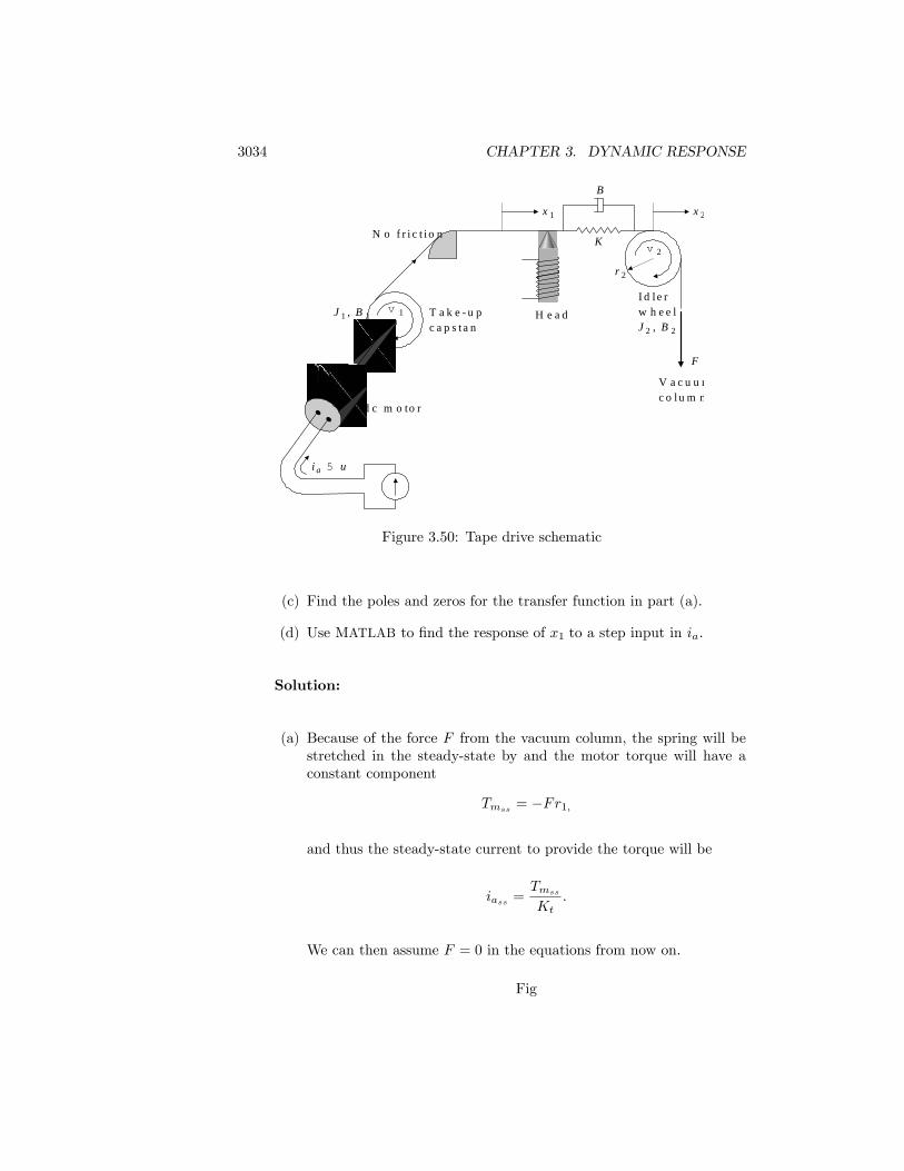
3034 CHAPTER 3. DYNAMIC RESPONSE
x 1 x 2
F
V a c u u mc o l u m n
r 1
r 2
H e a dv 1
v 2
T a k e u pc a p s t a n
i a 5 u
J 1 , B 1
N o f r i c t i o n
B
K
I d l e rw h e e lJ 2 , B 2
d c m o to r
Figure 3.50: Tape drive schematic
(c) Find the poles and zeros for the transfer function in part (a).
(d) Use MATLAB to �nd the response of x1 to a step input in ia.
Solution:
(a) Because of the force F from the vacuum column, the spring will bestretched in the steady-state by and the motor torque will have aconstant component
Tmss = �Fr1;
and thus the steady-state current to provide the torque will be
iass =Tmss
Kt:
We can then assume F = 0 in the equations from now on.
Fig

3035
17
9:pdf
Free body diagram for Problem 3.14.
On the capstan side:
Ktia|{z}Motor Torque
= J1 _!1| {z }Wheel Inertia
+ B1!1| {z }Wheel Damping
+r1[B( _x1 � _x2) + r1(x1 � x2)]| {z }Spring and damper
;
On the idler side:
Fr2|{z}Vac uum Col
= J2 _!2| {z }Wheel Inertia
+ B2!2| {z }Wheel Damping
+r2[�B( _x1 � _x2)�K(x1 � x2)]| {z }Spring and damper
:
We also have:
_x1 = r1!1;
_x2 = r2!2;
x1 = r1�1:
(b) From part (a):
J1 _!1 = �B1!1 +Ktia +Br1( _x2 � _x1) +Kr1(x2 � x1);J2 _!2 = �B2!2 +Br2( _x1 � _x2) +Kr2(x1 � x2);_x1 = r1!1;
_x2 = r2!2:
2664J1s+B1 0 (Bs+K)r1 �(Bs+K)r1
0 J2s+B2 �(Bs+K)r2 (Bs+K)r2�r1 0 s 00 �r2 0 s
37752664!1!2x1x2
3775 =2664KtIa000
3775 ;

3036 CHAPTER 3. DYNAMIC RESPONSE
X1(s)
Ia(s)=
Ktr1[J2s2 + (B2 + r
22B)s+ r
22K]
s
24 J1J2s3 + (J1B2 +B1J2 + r
22J1B + r
21J2B)s
2+(B1B2 + r
22J1K + r22B1B + r
21J2K + r21B2B)s
+r22B1K + r21B2K
35 ;
X1(s) =12(s+ 400)(s+ 1000)
s(s+ 380� j309)(s+ 1000)Ia(s) =num(s)
den(s)Ia(s):
(c)
Poles are at : 0; �380� j309; �1000;Zeros are at : � 400; �1000:
(d) The step response [step(num,den)] is shown in the �gure below.
0 0.005 0.01 0.015 0.02 0.025 0.030
1
2
3
4
5
6x 10 4
Time (sec)
Tape
pos
ition
0 0.005 0.01 0.015 0.02 0.025 0.030
1
2
3
4
5
6x 10 4
Time (sec)
Tape
pos
ition
Tape position response to a step in current.
15. For the system in Fig. 2.51, compute the transfer function from the motorvoltage to position �2.

3037
Solution:
From Problem 2.19:
Ldiadt+Raia + ke _�1 = va
ktia = J1��1 + b( _�1 � _�2) + k(�1 � �2) +B _�1J2��2 + b( _�2 � _�1) + k(�2 � �1) = 0
So we have:
LsIa(s) +RaIa(s) + ske�1(s) = Va(s);
ktIa(s) = s2J1�1(s) + b[�1(s)��2(s)]s+ k[�1(s)��2(s)] +Bs�1(s);
s2J2�2(s) + b[�2(s)��1(s)]s+ k[�2(s)��1(s)] = 0;
we have:
�2(s)
Va(s)=
kt(bs+ k)
det
24 ske 0 Ls+RaJ1s
2 +Bs+ bs+ k �bs� k �kt�bs� k J2s
2 + bs+ k 0
35 ;
=kt(bs+ k)
(Ls+Ra)[J1J2s4 + (J1b+BJ2 + bJ2)s
3 + (J1k +Bb+KJ2)s2 +Bks]
+kektJ2s3 + kektbs
2 + kkekts
;
=kt(bs+ k)
J1J2s5 + J2[J1Ra + L(b+B)]s
4
+[J2kektJ1L(b+ k) + LJ2k +Ra(b+B)J2 � Lb2]s3+[L(b+B)(b+ k)� 2bkL+ J1Ra(b+ k) +RaJ2k � b2Ra]s2
+[kekt(b+ k) + kL(b+ k)� bk2 +Ra(b+B)(b+ k)� 2bkRa]s+ kRab
:
16. Compute the transfer function for the two-tank system in Fig. 2.55 withholes at A and C.
Solution:
From Problem 2.23 but with s = a tank area we have:
��_h1�_h2
�=1
6a
��1 01 �1
� ��h1�h2
�+!ina
�10
�+
� �103a0
�;

3038 CHAPTER 3. DYNAMIC RESPONSE
�_h1 =��h1 + 6!in � 20
6a;
�_h2 =1
6a(�h1 ��h2);
s�h1(s) =��h1(s) + 6!in(s)
6a;
s�h2(s) =1
6a[�h1(s)��h2(s)];
�h2(s) =!in(s)
6a[a( 16a + s)]2;
�h2(s)
!in(s)=
1
6[a( 16a + s)]2:
17. For a second-order system with transfer function
G(s) =3
s2 + 2s� 3 ;
determine the following:
(a) The DC gain;
(b) The �nal value to a step input.
Solution:
(a) DC gain G(0) = 3�3 = �1
(b) limt!1
y(t) =?
s2 + 2s+ 3 = 0 =) s = 1;�3Since the system has an unstable pole, the Final Value Theorem isnot applicable. The output is unbounded.
18. Consider the continuous rolling mill depicted in Fig. 3.51. Suppose thatthe motion of the adjustable roller has a damping coe¢ cient b, and that theforce exerted by the rolled material on the adjustable roller is proportionalto the material�s change in thickness: Fs = c(T �x). Suppose further thatthe DC motor has a torque constant Kt and a back-emf constant Ke, andthat the rack-and-pinion has e¤ective radius of R.
(a) What are the inputs to this system? The output?
(b) Without neglecting the e¤ects of gravity on the adjustable roller,draw a block diagram of the system that explicitly shows the follow-ing quantities: Vs(s), I0(s); F (s) (the force the motor exerts on theadjustable roller), and X(s).

3039
1
2
i o ( t )
2
1
v a ( t ) v s ( t )
1 : NG e a r r a t i o
R a c k a n dP i n i o n
M o t io n o fm a t e r i a lo u t o f r o l l e r s
T h i c k n e s s TT h i c k n e s s x
V e r t i c a l l ya d j u s t a b l er o l l e r
F ix e dr o l l e r
L a R a
F m
Figure 3.51: Continuous rolling mill
(c) Simplify your block diagram as much as possible while still identifyingoutput and each input separately.
Solution:
(a)
Inputs: input voltage �! vs(t)
thickness �! T
gravity �! mg
Output: thickness �! x
(b) Dynamic analysis of adjustable roller:
m�x = c(T � x)�mg � b _x� Fm;
=) (s2m+ sb+ c)X(s) + Fm(s) +mg � cT
s= 0: (1)
Torque in rack and pinion:
TRP = RFm = NTmotor;
but Tmotor = KtIf io;
Fm =NKtIfR
io (2)

3040 CHAPTER 3. DYNAMIC RESPONSE
DC motor circuit analysis:
vs(t) = Raio + Ladiodt+ va(t);
va(t) = ue _�;
�R
N= x;
Io(s) =Vs(s)� KeN
R sX(s)
Ra + sLa(3)
Combining (1), (2), and (3):
0 = (s2m+ sb+ c)X(s)+mg � cT
s+NKtIfR
"Vs(s)� KeN
R sX(s)
sLa +Ra
#:
Block diagrams for rolling mill.

3041
Problems and Solutions for Section 3.2: Sys-tem Modeling Diagrams
19. Consider the block diagram shown in Fig. 3.52. Note that ai and bi areconstants. Compute the transfer function for this system. This spe-cial structure is called the �control canonical form�and will be discussedfurther in Chapter 7.)
S1
11
S
1
1 11
U ( s )
2 a 1
X 1
b 1
2 a 2
2 a 3
b 2
b 3
Y ( s )
1s
1s
X 2 X 31s
Figure 3.52: Block diagram for Problem 3.19
Solution:
We move the picko¤ point at X1 to the right past the second integratorto get b1s+ b2 as shown in the �gure on the next page.

3042 CHAPTER 3. DYNAMIC RESPONSE
Block diagram reduction for Problem 3.19.
We then move the picko¤ point at X2 past the third integrator to gets(b1s+b2)+b3. We have a block with the transfer function b1s2+b2s+b3at the output. Meanwhile we apply the feedback rule to the �rst innerloop to get 1
s+a1as shown in the �gure and repeat for the second and third
loops. We �nally have:
Y
U=
b1s2 + b2s+ b3
s3 + a1s2 + a2s+ a3:
Example on the web in Chapter 3 shows that we can obtain the sameanswer using Mason�s rule.
20. Find the transfer functions for the block diagrams in Fig. 3.53.
Solution:
(a)Block diagram for Fig. 3.53 (a)
Y
R=
G11 +G1
+G2:

3043
G 1S
2
G 2
S YR
( a )
G 1S
2
G 7
S YR
( b )
G 3
G 2
G 4S
2
G 6
G 5
G 1G 1 S
2 2
1
G 6
1
S YR
G 7
G 2 G 3 S
11
11
G 4 G 5
( c )
1
1 11
11
Figure 3.53: Block diagrams for Problem 3.20
(b)
Block diagram for Fig. 3.53 (b)
Block diagram for Fig. 3.53 (b): reduced

3044 CHAPTER 3. DYNAMIC RESPONSE
Y
R= G7 +
G1G3G4G6(1 +G1G2)(1 +G4G5)
:
(c)
Top: Block diagram for Fig. 3.53 (c) ; Bottom: Block diagram forFig 3.43 (c) reduced.
Y
R= G7 +
G6G4G51 +G4
+G1G2G31 +G2
� G4G51 +G4
:
21. Find the transfer functions for the block diagrams in Fig. 3.54, using theideas of block diagram simpli�cation. The special; structure in Fig. 3.54(b) is called the �observer canonical form�and will be discussed in Chap-ter 7.
Solution:
Part (a): Transfer functions found using the ideas of Figs. 3.8 and 3.9:
(a)(a) Block diagram for Fig. 3.54 (a).

3045
S
1
2
G 1R G 2S
1
1
S
11
H 2
G 3
H 3
S1
1
Y
(a )
S
1
2
b 3
a 3
1s S
1
2
11
b 2
a 2
1s S
1
2
b 1
a 1
1s
R
Y
( b )
S
1
2 22
a 1
a 2
a 3
1s
b 3
S
11
1
b 2
1s S
1
b 1
1s Y
R
S
1
2
R ( s ) S
1
2
S
11
Y ( s )
D ( s )
B ( s )
H ( s )
A ( s )
G ( s )
( c )
(d )
Figure 3.54: Block diagrams for Problem 3.21
G�2 =G2
1�G2H2;
G�3 =G3
1�G3H3;
Y
R=
G1(1 +G�2)
1 +G1(1 +G�2)G�3
=G1(1�G2H2)(1�G3H3) +G1G2(1�G3H3)
1 + (1�G2H2)(1�G3H3) +G1G3(1�G2H2) +G1G2G3:
(b) We move the summer on the right past the integrator to get b1s andrepeat to get (b2 + b1s)s. Meanwhile we apply the feedback rule tothe �rst inner loop to get 1
s+a1as shown in the �gure and repeat for
the second and third loops to get:

3046 CHAPTER 3. DYNAMIC RESPONSE
(b) Block diagram for Fig. 3.54(b).
Y
R=
b1s2 + b2s+ b3
s3 + a1s2 + a2s+ a3:
(c) Applying block diagram reduction: reduce innermost loop, shift b2 tothe b3 node, reduce next innermost loop and continue systematicallyto obtain:
(c) Block diagram for Fig. 3.54(c).

3047
(c) Block diagram for Fig. 3.54(c).
Y
R=b1s
2 + (a1b1 + b2)s+ a1b2 + a2b1 + b3s3 + a1s2 + a2s+ a3
:
(d)
(d) Block diagram for Fig. 3.54(d).
Y
R=
D +AB�
1 +G(D +AB�)=
D +DBH +AB
1 +BH +GD +GBDH +GAB:
22. Use block-diagram algebra to determine the transfer function betweenR(s) and Y(s) in Fig. 3.55.
Solution:

3048 CHAPTER 3. DYNAMIC RESPONSE
S
2
2
1
S
1
1
R ( s ) G 1
H 1
H 2
G 3
H 3
S
2
1
Y ( s )G 2
Figure 3.55: Block diagram for Problem 3.22
Block diagram for Fig. 3.55.
Move node A and close the loop:
Block diagram for Fig. 3.55: reduced.

3049
Add signal B, close loop and multiply before signal C:
Block diagram for Fig. 3.55: reduced.
Move middle block N past summer:
Block diagram for Fig. 3.55: reduced.
Now reverse order of summers and close each block separately:
Block diagram for Fig. 3.55: reduced.
Y
R=
feedforwardz }| {(N +G3) (
1
1 +NH3)| {z }
feedback
:

3050 CHAPTER 3. DYNAMIC RESPONSE
Y
R=G1G2 +G3(1 +G1H1 +G1H2)
1 +G1H1 +G1H2 +G1G2H3:
Problems and Solutions for Section 3.3: E¤ectof Pole Locations
23. For the electric circuit shown in Fig. 3.56, �nd the following:
(a) The time-domain equation relating i(t) and v1(t);
(b) The time-domain equation relating i(t) and v2(t);
(c) Assuming all initial conditions are zero, the transfer function V2(s)=V1(s)and the damping ratio � and undamped natural frequency !n of thesystem;
(d) The values of R that will result in v2(t) having an overshoot of nomore than 25%, assuming v1(t) is a unit step, L = 10 mH, andC = 4 �F.
L R
C v 2 ( t )v 1 ( t ) i ( t )
1
2
1
2
Figure 3.56: Circuit for Problem 3.23
Solution:
(a)
v1(t) = Ldi
dt+Ri+
1
C
Zi(t)dt:
(b)
v2(t) =1
C
Zi(t)dt:
(c)
v2(s)
v1(s)=
1sC
sL+R+ 1sC
=1
s2LC + sRC + 1:
(d) For 25% overshoot � t 0:4,

3051
0:4 t � =R
2q
LC
R = 2�
rL
C= (2)(0:4)
r10� 10�34� 10�6 = 40 :
24. For the unity feedback system shown in Fig. 3.57, specify the gain K ofthe proportional controller so that the output y(t) has an overshoot of nomore than 10% in response to a unit step.
KS
1
2
s ( s 1 2 )1R ( s ) Y ( s )
Figure 3.57: Unity feedback system for Problem 3.24
Solution:
Y (s)
R(s)=
K
s2 + 2s+K=
!2ns2 + 2�!ns+ !2n
;
!n =pK;
� =2
2!n=
1pK: (1)
In order to have an overshoot of no more than 10%:
Mp = e���=p1��2 � 0:10:
Solving for � :
� =
s(lnMp)2
�2 + (lnMp)2� 0:591:
Using (1) and the solution for �:
K =1
�2� 2:86;
) 0 < K � 2:86:

3052 CHAPTER 3. DYNAMIC RESPONSE
0 1 2 3 4 5 6 7 8 9 100
0.2
0.4
0.6
0.8
1
1.2
1.4
Step Response
Time (sec)
Ampl
itude
0 1 2 3 4 5 6 7 8 9 100
0.2
0.4
0.6
0.8
1
1.2
1.4
System: sy sTime (sec): 2.29Amplitude: 1.1
Step responses for K = 1 (blue) and K = 2:86 (green).
25. For the unity feedback system shown in Fig. 3.58, specify the gain andpole location of the compensator so that the overall closed-loop responseto a unit-step input has an overshoot of no more than 25%, and a 1%settling time of no more than 0.1 sec. Verify your design using Matlab.
S
1
2
s 1 2 51 0 0R ( s ) Y ( s )s 1 a
KC o m p e n s a t o r P l a n t
Figure 3.58: Unity feedback system for Problem 3.25
Solution:

3053
Y (s)
R(s)=
100K
s2 + (25 + a)s+ 25a+ 100K=
100K
s2 + 2�!ns+ !2n:
Using the given information:
R(s) =1
sunit step,
Mp � 25%;
ts � 0:1 sec :
Solve for � :
Mp = e���=p1��2 ;
� =
s(lnMp)2
�2 + (lnMp)2� 0:4037:
Solve for !n:
e��!nts = 0:01 For a 1% settling time.
ts �4:605
�!n= 0:1;
=) !n t 114:07:
Now �nd a and K :
2�!n = (25 + a);
a = 2�!n � 25 = 92:10� 25 = 67:10;!2n = (25a+ 100K);
K =!2n � 25a100
t 113:34:
The step response of the system using Matlab is shown below.

3054 CHAPTER 3. DYNAMIC RESPONSE
0 0.05 0.1 0.15 0.20
0.2
0.4
0.6
0.8
1
1.2
1.4
Time (sec)
y(t)
Step Response
0 0.05 0.1 0.15 0.20
0.2
0.4
0.6
0.8
1
1.2
1.4
Time (sec)
y(t)
Step Response
Step response for Problem 3.25.
Problems and Solutions for Section 3.4: Time-Domain Speci�cations
26. Suppose you desire the peak time of a given second-order system to beless than t0p. Draw the region in the s-plane that corresponds to values ofthe poles that meet the speci�cation tp < t0p.
Solution:

3055
s-plane region to meet peak time constraint: shaded.
!dtp = � =) tp =�
!d< t
0
p;
�
t0p< !d:
27. A certain servomechanism system has dynamics dominated by a pair ofcomplex poles and no �nite zeros. The time-domain speci�cations on therise time (tr), percent overshoot
(Mp), and settling time (ts) are given by,
tr � 0:6 sec ,
Mp � 17%,
ts � 9:2 sec .
(a) Sketch the region in the s-plane where the poles could be placedso that the system will meet all three speci�cations.
(b) Indicate on your sketch the speci�c locations (denoted by �) thatwill have the smallest rise-time and also meet the settling time speci�cationexactly.
Solution:
(a)-(b)

3056 CHAPTER 3. DYNAMIC RESPONSE
s-plane region to meet the speci�cations.
28. Suppose you are to design a unity feedback controller for a �rst-order plantdepicted in Fig. 3.59. (As you will learn in Chapter 4, the con�gurationshown is referred to as a proportional-integral controller.) You are todesign the controller so that the closed-loop poles lie within the shadedregions shown in Fig. 3.60.
KS
1
2
sK I
R YS
1
1
s 1 aK a
e ( t )
Figure 3.59: Unity feedback system for Problem 3.28

3057
R e ( s )
I m ( s )
2 22 4
2
4u 1
u 2
2 2
Figure 3.60: Desired closed-loop pole locations for Problem 3.28
(a) What values of !n and � correspond to the shaded regions in Fig. 3.60?(A simple estimate from the �gure is su¢ cient.)
(b) Let K� = � = 2. Find values for K and KI so that the poles of theclosed-loop system lie within the shaded regions.
(c) Prove that no matter what the values of K� and � are, the controllerprovides enough �exibility to place the poles anywhere in the complex(left-half) plane.
Solution:
(a) The values could be worked out mathematically but working fromthe diagram:
p32 + 22 = 3:6 =) 2:6 � !n � 4:6;
� = sin�1 �;
� = sin �:
From the �gure:
� t 34 � �1 = 0:554;
� t 70 � �2 = 0:939;
=) 0:6 � � � 0:9 (approximately)
(b) Closed-loop pole positions:
s(s+ �) + (Ks+KKI)K� = 0;
s2 + (�+KK�)s+KKIK� = 0:

3058 CHAPTER 3. DYNAMIC RESPONSE
For this case:
s2 + (2 + 2K)s+ 2KKI = 0 (�)
Choose roots that lie in the center of the shaded region,
(s+ (3 + j2))(s+ (3� j2)) = s2 + 6s+ 13 = 0;s2 + (2 + 2K)s+ 2KKI = s
2 + 6s+ 13;
2 + 2K = 6 =) K = 2;
13 = 4KI =) KI =13
4:
(c) For the closed-loop pole positions found in part (b), in the (*) equa-tion the value of K can be chosen to make the coe¢ cient of s takeon any value. For this value of K a value of KI can be chosen sothat the quantity KKIK� takes on any value desired. This impliesthat the poles can be placed anywhere in the complex plane.
29. The open-loop transfer function of a unity feedback system is
G(s) =K
s(s+ 2):
The desired system response to a step input is speci�ed as peak timetp = 1 sec and overshoot Mp = 5%.
(a) Determine whether both speci�cations can be met simultaneously byselecting the right value of K.
(b) Sketch the associated region in the s-plane where both speci�cationsare met, and indicate what root locations are possible for some likelyvalues of K.
(c) Pick a suitable value for K, and use Matlab to verify that the spec-i�cations are satis�ed.
Solution:
(a)
T (s) =Y (s)
R(s)=
G(s)
1 +G(s)=
K
s2 + 2s+K=
!2ns2 + 2�!ns+ !2n
:
Equate the coe¢ cients of like powers of s:
2 = 2�!nK = !2n
(*)
=) !n =pK � =
1pK:

3059
We would need:
Mp%
100= 0:05 = e
���p1��2 =) � = 0:69;
tp = 1 sec =�
!d=
�
!np1� �2
=) !n = 4:34:
But the combination (� = 0:69 , !n = 4:34) that we need is notpossible by varying K alone. Observe that from equations (*) �!n =1 6= 0:69� 4:34:
(b) Now we wish to have:
M�p = r � 0:05 = e
���p1��2
t�p = r � 1 sec = �!d
(**)
where r � relaxation factor.Recall the conditions of our system:
!n =pK;
� =1pK;
replace !n and � in the system (**):
=)� �p
K�1 = r � 0:051 sec = �p
K�1
=) r � 0:05 = e�r =) r �= 2:21:
K = 1 +�2
r2=) K = 3:02:
then with K = 3:02 we will have:
M�p = rMp = 2:21� 0:05 = 0:11:t�p = rtp = 2:21� 1 sec = 2:21 sec :
Note: * denotes actual location of closed-loop roots.

3060 CHAPTER 3. DYNAMIC RESPONSE
s-plane regions.
% Problem 3.29 FPE6eK=3.02;num=[K];den=[1, 2, K];sys=tf(num,den);t=0:.01:7;y=step(sys,t);plot(t,y);yss = dcgain(sys);Mp = (max(y) - yss)*100;% Finding maximum overshootmsg_overshoot = sprintf(�Max overshoot = %3.2f%%�, Mp);% Finding peak timeidx = max(�nd(y==(max(y))));tp = t(idx);msg_peaktime = sprintf(�Peak time = %3.2f�, tp);xlabel(�Time (sec)�);ylabel(�y(t)�);msg_title = sprintf(�Step Response with K=%3.2f�,K);title(msg_title);text(1.1, 0.3, msg_overshoot);

3061
text(1.1, 0.1, msg_peaktime);grid on;
0 1 2 3 4 5 6 70
0.2
0.4
0.6
0.8
1
1.2
1.4
Time (sec)
y(t)
Step Response with K=3.02
Max overshoot = 10.97%
Peak time = 2.21
0 1 2 3 4 5 6 70
0.2
0.4
0.6
0.8
1
1.2
1.4
Time (sec)
y(t)
Step Response with K=3.02
Max overshoot = 10.97%
Peak time = 2.21
Problem 3.29: Closed-loop step response.
30. NThe equations of motion for the DC motor shown in Fig. 2.32 were givenin Eqs. (2.52-53) as
Jm��m +
�b+
KtKe
Ra
�_�m =
Kt
Rava:
Assume that
Jm = 0:01 kg �m2;b = 0:001 N �m � sec;
Ke = 0:02 V � sec;Kt = 0:02 N �m=A;Ra = 10 :

3062 CHAPTER 3. DYNAMIC RESPONSE
(a) Find the transfer function between the applied voltage va and themotor speed _�m.
(b) What is the steady-state speed of the motor after a voltage va = 10 Vhas been applied?
(c) Find the transfer function between the applied voltage va and theshaft angle �m.
(d) Suppose feedback is added to the system in part (c) so that it becomesa position servo device such that the applied voltage is given by
va = K(�r � �m);
where K is the feedback gain. Find the transfer function between �rand �m.
(e) What is the maximum value of K that can be used if an overshootMp < 20% is desired?
(f) What values of K will provide a rise time of less than 4 sec? (Ignorethe Mp constraint.)
(g) Use Matlab to plot the step response of the position servo systemfor values of the gain K = 0:5, 1, and 2. Find the overshoot and risetime for each of the three step responses by examining your plots.Are the plots consistent with your calculations in parts (e) and (f)?
Solution:
Jm��m +
�b+
KtKe
Ra
�_�m =
Kt
Rava:
(a)
Jm�ms2 +
�b+
KtKe
Ra
��ms =
Kt
RaVa(s)
s�m(s)
Va(s)=
Kt
RaJm
s+ bJm+ KtKe
RaJm
:
Jm = 0:01 kg �m2;b = 0:001 N �m� sec;
Ke = 0:02 V� sec;Kt = 0:02 N �m=A;Ra = 10 :
s�m(s)
Va(s)=
0:2
s+ 0:104:

3063
(b) Final Value Theorem
_�(1) = s(10)(0:2)
s(s+ 0:104)js=0 =
2
0:104= 19:23:
(c)�m(s)
Va(s)=
0:2
s(s+ 0:104):
(d)
�m(s) =0:2K(�r ��m)s(s+ 0:104)
:
�m(s)
�r(s)=
0:2K
s2 + 0:104s+ 0:2K:
(e)
Mp = e���=p1��2 = 0:2 (20%);
� = 0:4559:
Y (s) =!2n
s2 + 2�!ns+ !2n:
2�!n = 0:104;
!n =0:104
2(0:4559)= 0:114 rad= sec;
!2n = 0:2K;
K < 6:50� 10�2:
(f)
!n � 1:8
tr
!2n = 0:2K
K � 1:01:
(g) Matlab% Problem 3.30 FPE6eclear allclose allK1=[0.5 1.0 2.0 6.5e-2];t=0:0.01:150;for i=1:1:length(K1)K = K1(i);titleText = sprintf(�K= %1.4f �, K);

3064 CHAPTER 3. DYNAMIC RESPONSE
wn = sqrt(0.2*K);num=wn^2;den=[1 0.104 wn^2];zeta=0.104/2/wn;sys = tf(num, den);y= step(sys, t);% Finding maximum overshootif zeta < 1Mp = (max(y) - 1)*100;overshootText = sprintf(�Max overshoot = %3.2f %�, Mp);elseovershootText = sprintf(�No overshoot�);end% Finding rise timeidx_01 = max(�nd(y<0.1));idx_09 = min(�nd(y>0.9));t_r = t(idx_09) - t(idx_01);risetimeText = sprintf(�Rise time = %3.2f sec�, t_r);% Plottingsubplot(3,2,i);plot(t,y);grid on;title(titleText);text( 0.5, 0.3, overshootText);text( 0.5, 0.1, risetimeText);end%%%%%%%%%%%%%%%%% Function for computing rise timefunction tr = risetime(t,y)% A. Emami 2006% normalize y to 1:y = y/y(length(y));idx1 = min(�nd(y>=0.1))idx2 = min(�nd(y>=0.9))if ~isempty(idx1) & ~isempty(idx2)tr = t(idx2) - t(idx1);elsetr = 0end

3065
0 50 100 1500
1
2 K= 0.4000
Max overshoot = 55.57 % Rise time = 4.20 sec
0 50 100 1500
1
2 K= 0.5000
Max overshoot = 59.23 % Rise time = 3.70 sec
0 50 100 1500
1
2 K= 1.0000
Max overshoot = 69.23 % Rise time = 2.51 sec
0 50 100 1500
1
2 K= 2.0000
Max overshoot = 77.17 % Rise time = 1.73 sec
0 50 100 1500
0.5
1
1.5 K= 0.0650
Max overshoot = 19.99 % Rise time = 13.66 sec
0 50 100 1500
1
2 K= 0.4000
Max overshoot = 55.57 % Rise time = 4.20 sec
0 50 100 1500
1
2 K= 0.5000
Max overshoot = 59.23 % Rise time = 3.70 sec
0 50 100 1500
1
2 K= 1.0000
Max overshoot = 69.23 % Rise time = 2.51 sec
0 50 100 1500
1
2 K= 2.0000
Max overshoot = 77.17 % Rise time = 1.73 sec
0 50 100 1500
0.5
1
1.5 K= 0.0650
Max overshoot = 19.99 % Rise time = 13.66 sec
Problem 3.30: Closed-loop step responses for several values of K.
For part (e) we concluded that K < 6:50 � 10�2 in order for Mp <20%: This is consistent with the above plots. For part (f) we foundthat K � 1:01 in order to have a rise time of less than 4 seconds.We actually see that our calculations is slightly o¤ and that K canbe K � 0:5, but since K � 1:01 is included in K � 0:5, our answerin part (f) is consistent with the above plots.
31. You wish to control the elevation of the satellite-tracking antenna shownin Figs. 3.61 and 3.62. The antenna and drive parts have a moment ofinertia J and a damping B; these arise to some extent from bearing andaerodynamic friction, but mostly from the back emf of the DC drive motor.The equations of motion are
J�� +B _� = Tc;
where Tc is the torque from the drive motor. Assume that
J = 600; 000 kg�m2 B = 20; 000 N�m�sec:

3066 CHAPTER 3. DYNAMIC RESPONSE
Figure 3.61: Satellite Antenna (Courtesy Space Systems/Loral)
(a) Find the transfer function between the applied torque Tc and theantenna angle �.
(b) Suppose the applied torque is computed so that � tracks a referencecommand �r according to the feedback law
Tc = K(�r � �);
where K is the feedback gain. Find the transfer function between �rand �.
(c) What is the maximum value of K that can be used if you wish tohave an overshoot Mp < 10%?
(d) What values of K will provide a rise time of less than 80 sec? (Ignorethe Mp constraint.)
(e) NUse Matlab to plot the step response of the antenna system forK = 200, 400, 1000, and 2000. Find the overshoot and rise timeof the four step responses by examining your plots. Do the plotscon�rm your calculations in parts (c) and (d)?
Solution:
J�� +B _� = Tc

3067
u
Figure 3.62: Schematic of antenna for Problem 3.31
(a)
J�s2 +B�s = Tc(s);
�(s)
Tc(s)=
1
s(Js+B);
J = 600; 000 kg �m2;B = 20; 000 N �m� sec;
�(s)
Tc(s)=
1:667� 10�6
s(s+ 130 )
:
(b)
�(s) =1:667� 10�6K(�r ��)
s(s+ 130 )
;
�(s)
�r(s)=
1:667K � 10�6
s2 + 130s+ 1:667K � 10�6
:

3068 CHAPTER 3. DYNAMIC RESPONSE
(c)
Mp = e���=p1��2 = 0:1 (10%);
� = 0:591:
Y (s) =!2n
s2 + 2�!ns+ !2n;
2�!n =1
30;
!n =130
2(0:591)= 0:0282 rad= sec;
!2n = 1:667K � 10�6;K < 477:
(d)
!n � 1:8
tr;
!2n = 1:667K � 10�6;K � 304:

3069
0 100 200 300 4000
0.5
1
1.5 K= 200.0000
Max overshoot = 0.08 Rise time = 161.10 sec
0 100 200 300 4000
0.5
1
1.5 K= 400.0000
Max overshoot = 7.03 Rise time = 76.30 sec
0 100 200 300 4000
0.5
1
1.5 K= 1000.0000
Max overshoot = 24.54 Rise time = 36.17 sec
0 100 200 300 4000
0.5
1
1.5 K= 2000.0000
Max overshoot = 38.78 Rise time = 22.64 sec
0 100 200 300 4000
0.5
1
1.5 K= 200.0000
Max overshoot = 0.08 Rise time = 161.10 sec
0 100 200 300 4000
0.5
1
1.5 K= 400.0000
Max overshoot = 7.03 Rise time = 76.30 sec
0 100 200 300 4000
0.5
1
1.5 K= 1000.0000
Max overshoot = 24.54 Rise time = 36.17 sec
0 100 200 300 4000
0.5
1
1.5 K= 2000.0000
Max overshoot = 38.78 Rise time = 22.64 sec
(e) Problem 3.31: Step responses for several values of K.
(e) The results compare favorably with the predictions made in parts(c) and (d). For K < 477 the overshoot was less than 10, the rise-time was less than 80 seconds.
32. (a) Show that the second-order system
�y + 2�!n _y + !2ny = 0; y(0) = yo; _y(0) = 0;
has the response
y(t) = yoe��tp1� �2
sin(!dt+ cos�1 �):
(b) Prove that, for the underdamped case (� < 1), the response oscilla-tions decay at a predictable rate (see Fig. 3.63) called the logarith-

3070 CHAPTER 3. DYNAMIC RESPONSE
Figure 3.63: De�nition of logarithmic decrement
mic decrement
� = lnyoy1= ��d
= ln�y1y1�= ln
�yiyi;
where�d =
2�
!d
is the damped natural period of vibration.
Solution:
(a) The system is second order =) Q(s) = s2+2�!ns+!2n. The initial
condition response can be obtained by plugging a dirac delta at theinput at the time 0 (this �charges� the system immediately to itsinitial condition and after that the system evolves by itself).
Inputeffective = y0�(t)
L�Inputeffective
�= y0
We do not know whether the transfer function has �nite zeros or not,but further thought will reveal the presence of at least one �nite zeroin the H(s).
lims!1
sH(s)y0 = y(t)j0+
where
H(s) =P (s)
Q(s)=
P (s)
s2 + 2�!ns+ !2n:

3071
If P (s) were a constant (no zeros in the H(s)), then the limit in theinitial value theorem would give always zero (which is wrong becausewe know that the initial value must be y0.) So we need a zero. Wesuggest using the following H(s):
H(s) =�s
s2 + 2�!ns+ !2n;
Y (s) = H(s)y0 =�sy0
s2 + 2�!ns+ !2n;
=R+
s� P++
R�s� P�
:
where
P+ = ��!n + j!nq1� �2;
P� = ��!n � j!nq1� �2;
R+ =�!nej(�=cos
�1 �)
2!np1� �2ej�=s
;
R� = R�+:
Note: The residues can be calculated graphically.
R+ = lims!P+
[(s� P+)Y (s)];
=) y(t) = R+eP+t +R�e
P�t
y(t) =�e��!nt
2p1� �2
he+j(!n
p1��2t+�=2�cos�1 �) + e�j(!n
p1��2t+�=2�cos�1 �)
i;
=) y(t) = y0e��tp1� �2
sin(!dt� cos�1 �):
(b)
dy(t)
dt= 0 =) t =
n�
!d(n is any integer)
tMax =2�
!dn
y(t)jtMax� yn = y0
e��n�dp1� �2
sin(cos�1 �):
Note:
sin(� cos�1 �) =q1� �2

3072 CHAPTER 3. DYNAMIC RESPONSE
yn =y0p1� �2p1� �2
e��n�d (�)
(Proof of the �rst line)
� = lny0yn= ��d;
From (*)
y1 = y0e���d =) ln
y0yn= ��d:
(Proof of the second line)
�yn = yn�1 � yn;�yn = y0e
��n�d � y0e�(n�1)��d = y0e��n�d(1� e��d);
=) �ynyn
=y0e
��n�d
y0e��n�d(1� e��d);
=) �ynyn
=�yiyi
for all i; n:
Problems and Solutions for Section 3.5: Ef-fects of Zeros and Additional Poles
33. In aircraft control systems, an ideal pitch response (qo) versus a pitchcommand (qc) is described by the transfer function
Qo(s)
Qc(s)=
�!2n(s+ 1=�)
s2 + 2�!ns+ !2n:
The actual aircraft response is more complicated than this ideal transferfunction; nevertheless, the ideal model is used as a guide for autopilotdesign. Assume that tr is the desired rise time and that
!n =1:789
tr,
1
�=1:6
tr,
� = 0:89.
Show that this ideal response possesses a fast settling time and minimalovershoot by plotting the step response for tr = 0:8, 1.0, 1.2, and 1.5 sec.
Solution:
The following program statements in Matlab produce the following plots:
% Problem 3.33 FPE6e

3073
tr = [0.8 1.0 1.2 1.5];
t=[1:240]/30;
tback=�iplr(t);
clf;
for I=1:4,
wn=(1.789)/tr(I); %Rads/second
tau=tr(I)/(1.6); %tau
zeta=0.89; %
b=tau*(wn^2)*[1 1/tau];
a=[1 2*zeta*wn (wn^2)];
y=step(b,a,t);
subplot(2,2,I);
plot(t,y);
titletext=sprintf(�tr=%3.1f seconds�,tr(I));
title(titletext);
xlabel(�t (seconds)�);
ylabel(�Qo/Qc�);
ymax=(max(y)-1)*100;
msg=sprintf(�Max overshoot=%3.1f%%�,ymax);
text(.50,.30,msg);
yback=�ipud(y);
yind=�nd(abs(yback-1)>0.01);
ts=tback(min(yind));
msg=sprintf(�Settling time =%3.1f sec�,ts);
text(.50,.10,msg);
grid;
end

3074 CHAPTER 3. DYNAMIC RESPONSE
0 2 4 6 80
0.5
1
1.5tr = 0.8 seconds
t (seconds)
Qo/
Qc
Max overshoot = 2.3%Settling time = 2.3 sec
0 2 4 6 80
0.5
1
1.5tr = 1.0 seconds
t (seconds)
Qo/
Qc
Max overshoot = 2.3%Settling time = 2.9 sec
0 2 4 6 80
0.5
1
1.5tr = 1.2 seconds
t (seconds)
Qo/
Qc
Max overshoot = 2.3%Settling time = 3.5 sec
0 2 4 6 80
0.5
1
1.5tr = 1.5 seconds
t (seconds)
Qo/
Qc
Max overshoot = 2.3%Settling time = 4.4 sec
0 2 4 6 80
0.5
1
1.5tr = 0.8 seconds
t (seconds)
Qo/
Qc
Max overshoot = 2.3%Settling time = 2.3 sec
0 2 4 6 80
0.5
1
1.5tr = 1.0 seconds
t (seconds)
Qo/
Qc
Max overshoot = 2.3%Settling time = 2.9 sec
0 2 4 6 80
0.5
1
1.5tr = 1.2 seconds
t (seconds)
Qo/
Qc
Max overshoot = 2.3%Settling time = 3.5 sec
0 2 4 6 80
0.5
1
1.5tr = 1.5 seconds
t (seconds)
Qo/
Qc
Max overshoot = 2.3%Settling time = 4.4 sec
Problem 3.33: Ideal pitch response.
34. Consider the system shown in Fig. 3.64, where
G(s) =1
s(s+ 3)and D(s) =
K(s+ z)
s+ p: (1)
Find K, z, and p so that the closed-loop system has a 10% overshoot to astep input and a settling time of 1.5 sec (1% criterion).
D ( s )R ( s ) Y ( s )S
2
1
G ( s )
Figure 3.64: Unity feedback system for Problem 3.34
Solution:
For the 10% overshoot:

3075
Mp = e���=p1��2 = 10%
=) � =
s(lnMp)2
�2 + (lnMp)2= 0:
For the 1:5sec (1% criterion):
!n =4:6
�ts=
4:6
(0:6)(1:5)= 5:11:
The closed-loop transfer function is:
Y (s)
R(s)=
K s+zs+p �
1s(s+3)
1 +K s+zs+p �
1s(s+3)
=K(s+ z)
s(s+ 3)(s+ p) +K(s+ z):
Method I.
From inspection, if z = 3, (s + 3) will cancel out and we will have astandard form transfer function. As perfect cancellation is impossible,assign z a value that is very close to 3, say 3:1. But in determining the Kand p, assume that (s+ 3) and(s+ 3:1) cancelled out each other. Then:
Y (s)
R(s)=
K
s2 + ps+K
As the additional pole and zero will a¤ect the system response, pick somelarger damping ratio.
Let � = 0:7
!n =4:6
�ts=
4:6
(0:7)(1:5)= 4:38; so let !n = 4:5;
p = 2�!n = 2� 0:7� 4:5 = 6:3;K = !2n = 20:25:

3076 CHAPTER 3. DYNAMIC RESPONSE
0 0.2 0.4 0.6 0.8 1 1.2 1.4 1.6 1.8 20
0.2
0.4
0.6
0.8
1
1.2
1.4
Step Response
Time (sec)
Ampl
itude
0 0.2 0.4 0.6 0.8 1 1.2 1.4 1.6 1.8 20
0.2
0.4
0.6
0.8
1
1.2
1.4
System: sy sTime (sec): 0.955Amplitude: 1.05
Step response: Method I.
Method II.
There are 3 unknowns (z; p; K) and only 2 speci�ed conditions. We canarbitrarily choose p large such that complex poles will dominate in thesystem response.
Try p = 10z
Choose a damping ratio corresponding to an overshoot of 5% (instead of10%, just to be safe).
� = 0:707:
From the formula for settling time (with a 1% criterion)
!n =4:6
�ts=
4:6
0:707� 1:5 = 4:34;
adding some margin, let !n = 4:88: The characteristic equation is

3077
Q(s) = s3 + (3 + p) s2 + (3p+K)s+Kz = (s+ a)(s2 + 2�!ns+ !2n):
We want the characteristic equation to be the product of two factors, acouple of conjugated poles (dominant) and a non-dominant real pole farform the dominant poles.
Equate the coe¢ cients of like powers of s in the expressions of the char-acteristic equation.
!2na = Kz;
2�!na+ !2n = 30z +K;
2�!n + a = 3 + 10z:
Solving the three equations we get
z = 5:77;
p = 57:7;
K = 222:45;
a = 53:79:

3078 CHAPTER 3. DYNAMIC RESPONSE
0 0.2 0.4 0.6 0.8 1 1.2 1.4 1.60
0.2
0.4
0.6
0.8
1
1.2
1.4
Step Response
Time (sec)
Ampl
itude
0 0.2 0.4 0.6 0.8 1 1.2 1.4 1.60
0.2
0.4
0.6
0.8
1
1.2
1.4
System: sy sTime (sec): 0.628Amplitude: 1.08
Step response: Method II.
35. NSketch the step response of a system with the transfer function
G(s) =s=2 + 1
(s=40 + 1)[(s=4)2 + s=4 + 1]:
Justify your answer on the basis of the locations of the poles and zeros.(Do not �nd inverse Laplace transform.) Then compare your answer withthe step response computed using Matlab.
Solution:
From the location of the poles, we notice that the real pole is a factor of20 away from the complex pair of poles. Therefore, the response of thesystem is dominated by the complex pair of poles.
G(s) � (s=2 + 1)
[(s=4)2 + s=4 + 1]:
This is now in the same form as equation (3.72) where � = 1, � = 0:5 and!n = 4: Therefore, Fig. 3.27 suggests an overshoot of over 70%. The step

3079
response is the same as shown in Fig. 3.26, for � = 1, with more than70% overshoot and settling time of 3 seconds. The Matlab plots belowcon�rm this.
% Problem 3.35 FPE 6e
num=[1/2, 1];
den1=[1/16, 1/4, 1];
sys1=tf(num,den1);
t=0:.01:3;
y1=step(sys1,t);
den=conv([1/40, 1],den1);
sys=tf(num,den);
y=step(sys,t);
plot(t,y1,t,y);
xlabel(�Time (sec)�);
ylabel(�y(t)�);
title(�Step Response�);
grid on;

3080 CHAPTER 3. DYNAMIC RESPONSE
0 0.5 1 1.5 2 2.5 30
0.2
0.4
0.6
0.8
1
1.2
1.4
1.6
1.8
Time (sec)
y(t)
Step Response
0 0.5 1 1.5 2 2.5 30
0.2
0.4
0.6
0.8
1
1.2
1.4
1.6
1.8
Time (sec)
y(t)
Step Response
Problem 3.35: Comparison of step responses: third-order system (green),second-order approximation (blue).
36. Consider the two nonminimum phase systems,
G1(s) = �2(s� 1)
(s+ 1)(s+ 2); (2)
G2(s) =3(s� 1)(s� 2)
(s+ 1)(s+ 2)(s+ 3): (3)
(a) Sketch the unit step responses for G1(s) and G2(s), paying closeattention to the transient part of the response.
(b) Explain the di¤erence in the behavior of the two responses as it relatesto the zero locations.
(c) Consider a stable, strictly proper system (that is,m zeros and n poles,where m < n). Let y(t) denote the step response of the system. Thestep response is said to have an undershoot if it initially starts o¤ inthe �wrong�direction. Prove that a stable, strictly proper system has

3081
an undershoot if and only if its transfer function has an odd numberof real RHP zeros.
Solution:
(a) For G1(s) :
Y1(s) =1
sG1(s) =
�2(s� 1)s(s+ 1)(s+ 2)
;
H(s) = k
Qj(s� zj)Ql(s� pl)
;
Rpi = lims!pi
[(s� pi)H(s)] = lims!pi
k
Qj(s� zj)Ql
l 6=i(s� pl)= k
Qj(pi � zj)Ql
l 6=i(pi � pl):
Each factor (pi � zj) or (pi � pl) can be thought of as a complexnumber (a magnitude and a phase) whose pictorial representation isa vector pointing to pi and coming from zj or pl respectively.The method for calculating the residue at a pole pi is:(1) Draw vectors from the rest of the poles and from all the zeros tothe pole pi.(2) Measure magnitude and phase of these vectors.(3) The residue will be equal to the gain, multiplied by the productof the vectors coming from the zeros and divided by the product ofthe vectors coming from the poles.In our problem:
Y1(s) =�2(s� 1)
s(s+ 1)(s+ 2)=R0s+
R�1(s+ 1)
+R�2(s+ 2)
=1
s� 4
s+ 1+
3
s+ 2;
y1(t) = 1� 4e�t + 3e�2t:
For G2(s) :
Y2(s) =3(s� 1)(s� 2)
s(s+ 1)(s+ 2)(s+ 3)=1
s+�9
(s+ 1)+
18
(s+ 2)+�10(s+ 3)
;
y2(t) = 1� 9e�t + 18e�2t � 10e�3t:
(b) The �rst system presents an �undershoot�. The second system, onthe other hand, starts o¤ in the right direction.The reasons for this initial behavior of the step response will be an-alyzed in part c.
In y1(t): dominant at t = 0 the term �4e�tIn y2(t): dominant at t = 0 the term 18e�2t

3082 CHAPTER 3. DYNAMIC RESPONSE
0 1 2 3 4 5 6 7 8 9 100.4
0.2
0
0.2
0.4
0.6
0.8
1
Step Response
Time (sec)
y1(t)
0 1 2 3 4 5 6 7 8 9 100.4
0.2
0
0.2
0.4
0.6
0.8
1
Figure 3.65: Problem 3.36: Step response for a non-minimum phase system withone real RHP zero.

3083
0 1 2 3 4 5 6 7 8 9 100.4
0.2
0
0.2
0.4
0.6
0.8
1
Step Response
Time (sec)
y2(t)
0 1 2 3 4 5 6 7 8 9 100.4
0.2
0
0.2
0.4
0.6
0.8
1
Figure 3.66: Problem 3.36: Step response of a non-minimum phase system withtwo real zeros in the RHP.

3084 CHAPTER 3. DYNAMIC RESPONSE
(c) The following concise proof is from Reference [1] (see also References[2]-[3]).Without loss of generality assume the system has unity DC gain(G(0) = 1) Since the system is stable, y(1) = G(0) = 1; and it isreasonable to assume y(1) 6= 0: Let us denote the pole-zero excess asr = n�m: Then, y(t) and its r� 1 derivatives are zero at t = 0, andyr(0) is the �rst non-zero derivative. The system has an undershootif yr(0)y(1) < 0: The transfer function may be re-written as
G(s) =
Qmi=1(1� s
zi)Qm+r
i=1 (1� spi)
The numerator terms can be classi�ed into three types of terms:(1). The �rst group of terms are of the form (1� �is) with �i > 0.(2). The second group of terms are of the form (1+�is) with �i > 0.(3). Finally, the third group of terms are of the form, (1+�is+�is
2)with �i > 0; and �i could be negative.However, �2i < 4�i; so that the corresponding zeros are complex.All the denominator terms are of the form (2), (3), above. Since,
yr(0) = lims!1
srG(s)
it is seen that the sign of yr(0) is determined entirely by the numberof terms of group 3 above. In particular, if the number is odd, thenyr(0) is negative and if it is even, then yr(0) is positive. Sincey(1) = G(0) = 1; then we have the desired result.References[1] Vidyasagar, M., �On Undershoot and Nonminimum Phase Zeros,�IEEE Trans. Automat. Contr., Vol. AC-31, p. 440, May 1986.[2] Clark, R., N., Introduction to Automatic Control Systems, JohnWiley, 1962.[3] Mita, T. and H. Yoshida, �Undershooting phenomenon and itscontrol in linear multivariable servomechanisms, �IEEE Trans. Au-tomat. Contr., Vol. AC-26, pp. 402-407, 1981.
37. Find the relationships for the impulse response and the step responsecorresponding to Equation (3.57) for the cases where,
(a) the roots are repeated.
(b) the roots are both real. Express your answers in terms of hyperbolicfunctions (sinh, cosh) to best show the properties of the system response.
(c) the value of the damping coe¢ cient, �, is negative.
Solution:

3085
(a) In this case we have � = 1
H(s) =Y (s)
U(s)=
!2n(s+ !n)2
:
For the impulse response,U(s) = 1, and using Item #8 from Table A.2 we�nd
h(t) = !2nte�!nt:
We can then integrate the impulse response to obtain the step response.Alternatively, for a unit step input, U(s) = 1
s and
Y (s) =!2n
(s+ !n)21
s:
Using Item #15 from Table A.2 we �nd
y(t) = 1� e�!nt (1 + !nt) :
(b) We re-write H(s) as follows
H(s) =Y (s)
U(s)=
!2n
(s+ �!n + !np�2 � 1)(s+ �!n � !n
p�2 � 1)
;
where j�j > 1. For the impulse response,U(s) = 1 and using Item #13from Table A.2,
h(t) = � !2n
2!np�2 � 1
�e�(�!n+!n
p�2�1)t � e�(�!n�!n
p�2�1)t
�;
=!n
2p�2 � 1
e��!nt�e+(!n
p�2�1)t � e�(!n
p�2�1)t
�;
=!np�2 � 1
e��!nt sinh(!n
q�2 � 1t):
We can then integrate the impulse response to obtain the unit step re-sponse. Alternatively, for a unit step input, U(s) = 1
s and using partialfraction expansion
Y (s) =1
s+
1
2p�2�1
��+p�2�1
�s+ �!n + !n
p�2 � 1
�
1
2p�2�1
���p�2�1
�s+ �!n � !n
p�2 � 1
;

3086 CHAPTER 3. DYNAMIC RESPONSE
and using Item #7 from Table A.2
y(t) = 1 +1
2p�2 � 1
�� +
p�2 � 1
�e�(�!n+!np�2�1)t� 1
2p�2 � 1
�� �
p�2 � 1
�e�(�!n�!np�2�1)t;= 1 +
1
2p�2 � 1
e��!nt
0@ 1�� +
p�2 � 1
�e�!np�2�1t � 1�� �
p�2 � 1
�e+!np�2�1t1A ;
= 1 +1
2p�2 � 1
e��!nt��� �
q�2 � 1
�e�!n
p�2�1t �
�� +
q�2 � 1
�e+!n
p�2�1t
�;
y(t) = 1� e��!nt cosh
��!n
q�2 � 1t
�+
�p�2 � 1
sinh
�!n
q�2 � 1t
�!:
Notice that unlike the expression for the impulse response on FPE 6epage 112 (Eq. 3.58) and the step response on FPE 6e page 117 (Eq.3.61), these responses do not oscillate due to the behavior of the cosh andsinh functions.
(c) Now we have the remaining case where � is negative and j�j < 1 , sincewe already dealt with the case of j�j > 1 in the previous part (b). Theimpulse response and the step responses are exactly the same as given inon pages 112 (Eq. 3.58) and 117 (Eq. 3.61)
h(t) =!np1� �2
e��t sin(!dt)
y(t) = 1� e��t�cos(!dt) +
�
!dsin(!dt)
�
except now � is negative and the exponential terms become unboundedand the system is unstable.
38. Consider the following second-order system with an extra pole:
H(s) =!2np
(s+ p)(s2 + 2�!ns+ !2n):
Show that the unit step response is
y(t) = 1 +Ae�pt +Be��t sin(!dt� �);

3087
where
A =�!2n
!2n � 2�!np+ p2;
B =pq
(p2 � 2�!np+ !2n)(1� �2);
� = tan�1p1� �2
�� + tan�1!np1� �2
p� �!n:
(a) Which term dominates y(t) as p gets large?
(b) Give approximate values for A and B for small values of p.
(c) Which term dominates as p gets small? (Small with respect to what?)
(d) Using the preceding explicit expression for y(t) or the step commandin Matlab, and assuming that !n = 1 and � = 0:7, plot the stepresponse of the preceding system for several values of p ranging fromvery small to very large. At what point does the extra pole cease tohave much e¤ect on the system response?
Solution:
Second-order system:
H(s) =!2np
(s+ p)(s2 + 2�!ns+ !2n):
Unit step response:
Y (s) =1
sH(s); y(t) = L�1fY (s)g;
s2 + 2�!ns+ !2n = (s+ � + j!d)(s+ � � j!d);
where
� = �!n; !d = !n
q1� �2:
Thus from partial fraction expansion:
Y (s) =k1s+
k2s+ p
+k3
s+ � + j!d+
k4s+ � � j!d
;

3088 CHAPTER 3. DYNAMIC RESPONSE
solving for k1; k2; k3; and k4:
k1 = H(0) =) k1 = 1;
k2 =!2np
s(s+ � + j!d)(s+ � � j!d)js=�p =) k2 =
�!2n!2n � 2p�!n + p2
;
k3 = (s+ � + j!d)Y (s)js=���j!d=) k3 =
p
2q(1� �2) (p2 � 2p�!n + !2n)
e�i� = jk3j e�i�
k4 = k�3
where
� = tan�1
p1� �2
��
!+ tan�1
!np1� �2
p� �!n
!:
Thus
Y (s) =1
s+
k2s+ p
+ jk3j�
e�i�
s+ � + j!d+
e+i�
s+ � � j!d
�:
Inverse Laplace:
y(t) = 1 + k2e�pt + jk3j
�e�i�e�(�+j!d)t + e+i�e�(��j!d)t
�;
or
y(t) = 1+�!2n
!2n � 2p�!n + p2| {z }A
e�pt+pq
(1� �2) (p2 � 2p�!n + !2n)| {z }B
e��t cos(!dt+�):
(a) As p gets large the B term dominates.
(b) For small p: A t �1; B t 0:
(c) As p gets small A dominates.
(d) The e¤ect of a change in p is not noticeable above p t 10:

3089
0 20 40 600
0.2
0.4
0.6
0.8
1 Step Response for p= 0.10
0 20 40 600
0.5
1
1.5 Step Response for p= 1.00
0 20 40 600
0.5
1
1.5 Step Response for p= 10.00
0 20 40 600
0.5
1
1.5 Step Response for p= 100.00
0 20 40 600
0.2
0.4
0.6
0.8
1 Step Response for p= 0.10
0 20 40 600
0.5
1
1.5 Step Response for p= 1.00
0 20 40 600
0.5
1
1.5 Step Response for p= 10.00
0 20 40 600
0.5
1
1.5 Step Response for p= 100.00
Problem 3.38: Step responses for several values of p.
39. Consider the second order unity DC gain system with one �nite zero,
H(s) =!2n(s+ z)
z(s2 + 2�!ns+ !2n):
(a) Show that the unit-step response is
y(t) = 1 +1
z
e��tp1� �2
p!2n + z
2 � 2�!n cos(!dt� �1);
where
�1 = tan�1 �z � !np
1� �2z:
(b) Derive an expression for the overshoot, Mp, for this system.
(c) For a given value of overshoot, Mp, how do we solve for � and !n?
Solution:

3090 CHAPTER 3. DYNAMIC RESPONSE
(a). We write the transfer function in partial fraction form,
H(s) =!2n
(s2 + 2�!ns+ !2n)+1
z
!2ns
(s2 + 2�!ns+ !2n):
The step response of the �rst term is as given in Chapter 3, and thatof the second term is simply the derivative of that (i.e., the impulseresponse) scaled by 1=z:
y(t) = y1 +1
z
dy1dt;
y(t) = 1� e��tp1� �2
cos(!dt� �) +1
z
"�e��tp1� �2
cos(!dt� �) +!de
��tp1� �2
sin(!dt� �)#;
y(t) = 1� e��tp1� �2
��1 + �
z
�cos(!dt� �) +
e��tp1� �2
!dzsin(!dt� �)
where � = tan�1�p1� �2
:
Now as in Chapter 3 we combine the last two terms to yield,
y(t) = 1 +1
z
e��tp1� �2
�p!2n + z
2 � 2�!n�cos(!dt� (� + �2));
where �2 = tan�1!np1� �2
�!n � z:
Using the trigonometric identity,
tan�1A+ tan�1B = tan�1A+B
1�AB ;
we combine the last two terms in the argument of the cosine term,
�1 = � + �2 = tan�1
0BB@�p1��2
+!np1��2
�!n�z
1� �p1��2
!np1��2
�!n�z
1CCA = tan�1�z � !np1� �2z
:
Hence we have the �nal desired result,
y(t) = 1 +1
z
e��tp1� �2
�p!2n + z
2 � 2�!n�cos(!dt� �1):
Alternative Solution for (a):

3091
y(t) = y1 +1
z
dy1dt;
= 1� e��tp1� �2
cos(!dt� �) +1
z
"!ne
��tp1� �2
sin(!dt)
#;
= 1� e��tp1� �2
�(�!nz
+ sin(�)) sin(!dt) + cos(!dt) cos(�)
�;
where � = tan�1�p1� �2
:
cos(�) = cos
tan�1
�p1� �2
!=
1s1 +
��p1��2
�2 =q1� �2;
sin(�) = sin
tan�1
�p1� �2
!=
�p1��2s
1 +
��p1��2
�2 = �;
y(t) = 1� e��tp1� �2
�(�!nz
+ �) sin(!dt) +
q1� �2 cos(!dt)
�;
y(t) = 1� e��tp1� �2
24s(�!nz
+ �)2 +
�q1� �2
�2cos(!dt� �1)
35 ;y(t) = 1� e��tp
1� �2
"r(�!nz
+ �)2 + 1� �2 cos(!dt� �1)#;
y(t) = 1 +1
z
e��tp1� �2
p!2n + z
2 � 2�!n cos(!dt� �1);
where �1 = tan�1�z � !np1� �2z
:
(b) At peak time tp, we have that
dy(tp)
dt= 0;
��z
e��tp1� �2
�p!2n + z
2 � 2�!n�cos(!dt� �1)�
!dz
e��tp1� �2
�p!2n + z
2 � 2�!n�sin(!dt� �1) = 0;

3092 CHAPTER 3. DYNAMIC RESPONSE
cos(!dt� �1 � �3) = 0;
�3 = tan�1p1� �2
�;
�1 + �3 = tan�1
�z�!np1��2z
+
p1��2�
1� �z�!np1��2z
p1��2�
= tan�1�z � !n!n
�;
tp =1
!d
"tan�1
z � �!n!np1� �2
!+3
2�
#;
Mp = y(tp)� 1;
Mp =1
z
pz2 � z�!n + !2ne��tp :
(c) For a given overshoot Mp, the values of !n and � have to befound by trial and error. In general, they will be di¤erent than thestandard second order system values unless z is large that is the zerois far away.
40. The block diagram of an autopilot designed to maintain the pitch attitude� of an aircraft is shown in Fig. 3.67. The transfer function relating theelevator angle �e and the pitch attitude � is
�(s)
�e(s)= G(s) =
50(s+ 1)(s+ 2)
(s2 + 5s+ 40)(s2 + 0:03s+ 0:06);
where � is the pitch attitude in degrees and �e is the elevator angle indegrees. The autopilot controller uses the pitch attitude error e to adjustthe elevator according to the transfer function
�e(s)
e(s)= D(s) =
K(s+ 3)
s+ 10:
Using Matlab, �nd a value of K that will provide an overshoot of lessthan 10% and a rise time faster than 0:5 sec for a unit-step change in �r.After examining the step response of the system for various values of K,comment on the di¢ culty associated with making rise-time and overshootmeasurements for complicated systems.
Solution:
G(s) =�(s)
�e(s)=
50 (s+ 1) (s+ 2)
(s2 + 5s+ 40) (s2 + 0:03s+ 0:06);
D(s) =�e(s)
e(s)=K(s+ 3)
(s+ 10);

3093
S
1
2
G ( s )
A i r c r a f t
D ( s )
C o n t r o ld eeu r
u
Figure 3.67: Block diagram of autopilot
where
e(s) = �r ��;�(s)
�r(s)=
G(s)D(s)
1 +G(s)D(s);
=50K (s+ 1) (s+ 2) (s+ 3)
(s2 + 5s+ 40) (s2 + 0:03s+ 0:06) (s+ 10) +K (s+ 3);
=50K
�s3 + 6s2 + 11s+ 6
�s5 + 15:03s4 + (50K + 90:51)s3 + (300K + 403:6)s2 + (17:4 + 550K) s+ (24 + 300K)
:
Output must be normalized to the �nal value of �(s)�r(s)
for easy computa-tion of the overshoot and rise-time. In this case the design criterion forovershoot cannot be met easily which is indicated in the sample plots.

3094 CHAPTER 3. DYNAMIC RESPONSE
0 50 100 1500
0.5
1
1.5 K= 3.5000
Time (sec)
θ
Max overshoot = 17.21 Rise time = 0.11 sec
0 50 100 1500
0.5
1
1.5 K= 3.0000
Time (sec)
θ
Max overshoot = 12.31 Rise time = 0.12 sec
0 50 100 1500
0.5
1
1.5 K= 0.3000
Time (sec)
θ
Max overshoot = 38.11 Rise time = 1.89 sec
0 50 100 1500
0.5
1
1.5
2 K= 0.0300
Time (sec)
θ Max overshoot = 73.67 Rise time = 3.61 sec
0 50 100 1500
0.5
1
1.5 K= 3.5000
Time (sec)
θ
Max overshoot = 17.21 Rise time = 0.11 sec
0 50 100 1500
0.5
1
1.5 K= 3.0000
Time (sec)
θ
Max overshoot = 12.31 Rise time = 0.12 sec
0 50 100 1500
0.5
1
1.5 K= 0.3000
Time (sec)
θ
Max overshoot = 38.11 Rise time = 1.89 sec
0 50 100 1500
0.5
1
1.5
2 K= 0.0300
Time (sec)
θ Max overshoot = 73.67 Rise time = 3.61 sec
Problem 3.40: Step responses for an autopilot for various values of K.
Problems and Solutions for Section 3.7: Sta-bility
41. A measure of the degree of instability in an unstable aircraft responseis the amount of time it takes for the amplitude of the time response todouble (see Fig. 3.68), given some nonzero initial condition.
(a) For a �rst-order system, show that the time to double is
�2 =ln 2
p;
where p is the pole location in the RHP.
(b) For a second-order system (with two complex poles in the RHP),show that
�2 =ln 2
��!n:

3095
T i m e
A m p l i t u d e
2 AA0
2 A
t 2
Figure 3.68: Time to double
Solution:
(a) First-order system, H(s) could be:
H(s) =k
(s� p) ;
h(t) = L�1 [H(s)] = kept;h(�0) = kep�0 ;
h (�0 + �2) = 2h (�0) = kep(�0+�2);
=) 2kep�0 = kep�0ep�2 ;
=) �2 =ln 2
p:
(b) Second-order system:
y (t) = y0e!nj�jtq1�
���2�� sin�!n
q1�
���2��t+ cos�1 �� ;where
cos�1 � = cos�1 j�j+ �
=) y (t) = y0e!nj�jtq1�
���2�� (�1) sin�!n
q1�
���2��t+ cos�1 j�j�
Note: Instead of working with a negative �; everything is changed toj�j.

3096 CHAPTER 3. DYNAMIC RESPONSE
jt0j = �y0e!nj�jtq1�
���2�� ;j�0j = �y0
e!nj�j�0q1�
���2�� ;j�0 + �2j = �y0
e!nj�j(�0+�2)q1�
���2�� = 2 j�0j
=) e!nj�j�2 = 2
=) �2 =ln 2
!n j�j=
ln 2
�!n�(� � 0)
Note: This problem shows that � = !n j�j (the real part of the poles)is inversely proportional to the time to double.
The further away from the imaginary axis the poles lie, the fasterthe response is (either increasing faster for RHP poles or decreasingfaster for LHP poles).
42. Suppose that unity feedback is to be applied around the listed open-loopsystems. Use Routh�s stability criterion to determine whether the resultingclosed-loop systems will be stable.
(a) KG(s) = 4(s+2)s(s3+2s2+3s+4)
(b) KG(s) = 2(s+4)s2(s+1)
(c) KG(s) = 4(s3+2s2+s+1)s2(s3+2s2�s�1)
Solution:
(a)1 +KG = s4 + 2s3 + 3s2 + 8s+ 8 = 0:
The Rouh array is,
s4 : 1 3 8
s3 : 2 8
s2 : a b
s1 : c
s0 : d

3097
where
a =2� 3� 8� 1
2= �1 b =
2� 8� 1� 02
= 8;
c =3a� 2ba
=�8� 16�1 = 24;
d = b = 8:
2 sign changes in the �rst column =) 2 roots not in the LHP=)unstable.
(b)1 +KG = s3 + s2 + 2s+ 8 = 0:
The Routh�s array is,
s3 : 1 2
s2 : 1 8
s1 : �6s0 : 8
There are two sign changes in the �rst column of the Routh array.Therefore, there are two roots not in the LHP.
(c)1 +KG = s5 + 2s4 + 3s3 + 7s2 + 4s+ 4 = 0:
The Routh array is,
s5 : 1 3 4
s4 : 2 7 4
s3 : a1 a2
s2 : b1 b2
s1 : c1
s0 : d1
where
a1 =6� 72
=�12
a2 =8� 42
= 2
b1 =�7=2� 4�1=2 = 15 b2 =
�4=2� 0�1=2 = 4
c1 =30 + 2
15=32
15d1 = 4
2 sign changes in the �rst column =) 2 roots not in the LHP =)unstable.

3098 CHAPTER 3. DYNAMIC RESPONSE
43. Use Routh�s stability criterion to determine how many roots with positivereal parts the following equations have:
(a) s4 + 8s3 + 32s2 + 80s+ 100 = 0.
(b) s5 + 10s4 + 30s3 + 80s2 + 344s+ 480 = 0.
(c) s4 + 2s3 + 7s2 � 2s+ 8 = 0.(d) s3 + s2 + 20s+ 78 = 0.
(e) s4 + 6s2 + 25 = 0.
Solution:
(a)s4 + 8s3 + 32s2 + 80s+ 100 = 0
The Routh array is,
s4 : 1 32 100
s3 : 8 80
s2 : 22 100
s1 : 80� 80022
= 43:6
s0 : 100
=) No roots not in the LHP
(b)s5 + 10s4 + 30s3 + 80s2 + 344s+ 480 = 0
s5 : 1 30 344
s4 : 10 80 480
s3 : 22 296
s2 : �545 480
s1 : 490
s0 : 480
=) 2 roots not in the LHP.
(c)s4 + 2s3 + 7s2 � 2s+ 8 = 0
There are roots in the RHP (not all coe¢ cients are >0). The Routharray is,

3099
s4 : 1 7 8
s3 : 2 � 2s2 : 8 8
s1 : �4s0 : 8
=) 2 roots not in the LHP.
(d) The Routh array is,
s3 : 1 20
s2 : 1 78
s1 : �58s0 : 78
There are two sign changes in the �rst column of the Routh array.Therefore, there are two roots not in the LHP.
(e)
a (s) = s4 + 6s2 + 25 = 0
Two coe¢ cients are missing so there are roots outside the LHP.
Create a new row by da(s)ds :
The Routh array with the new row is,
s4 : 1 6 25
s3 : 4 12 � new rows2 : 3 25
s1 : 12� 1003= �21:3
s0 : 25
=) 2 roots not in the LHP
check:
a (s) = 0 =) s2 = �3� 4j = 5ej(��0:92)
s =p5ej(
�2�0:46)+n�j n = 0; 1

3100 CHAPTER 3. DYNAMIC RESPONSE
Problem 3.43: s-plane pole locations.
44. Find the range of K for which all the roots of the following polynomialare in the LHP:
s5 + 5s4 + 10s3 + 10s2 + 5s+K = 0:
Use Matlab to verify your answer by plotting the roots of the polynomialin the s-plane for various values of K.
Solution:s5 + 5s4 + 10s3 + 10s2 + 5s+K = 0:
The Routh array is,
s5 : 1 10 5
s4 : 5 10 K
s3 : a1 a2
s2 : b1 K
s1 : c1
s0 : K
where
a1 =5 (10)� 1 (10)
5= 8 a2 =
5 (5)� 1 (K)5
=25�K8
b1 =(a1) (10)� (5) (a2)
a1=55 +K
8
c1 =(b1) (a2)� (a1) (K)
b1=��K2 + 350K � 1375
�5 (55 +K)

3101
For stability: all elements in �rst the �rst column must be positive thatresults in the following set of constraints:
(1) b1 =55 +K
8> 0 =) K > �55
(2) c1 =��K2 + 350K � 1375
�5 (55 +K)
> 0;� (K � 3:88) (K + 354)
5 (55 +K)> 0 =) �55 < K < 3:88
(3) d1 = K > 0
Combining (1), (2), and (3) =) 0 < K < 3:88: If we plot the roots ofthe polynomial for various values of K we obtain the following root locusplot (see Chapter 5),
Root Locus
Real Axis
Imag
Axi
s
3 2.5 2 1.5 1 0.5 0 0.5 1
2
1.5
1
0.5
0
0.5
1
1.5
2
K=0
K=0
K=0
K=0
K=0K=1
K=3.88
K=3.88
Problem 3.44: Roots of the polynomial in the s-plane for various valuesof K.
45. The transfer function of a typical tape-drive system is given by
G(s) =K(s+ 4)
s[(s+ 0:5)(s+ 1)(s2 + 0:4s+ 4)];
where time is measured in milliseconds. Using Routh�s stability crite-rion, determine the range of K for which this system is stable when thecharacteristic equation is 1 +G(s) = 0.
Solution:
1 +G (s) = s5 + 1:9s4 + 5:1s3 + 6:2s2 + (2 +K) s+ 4K = 0:

3102 CHAPTER 3. DYNAMIC RESPONSE
The Routh array is,
s5 : 1:0 5:1 2 +K
s4 : 1:9 6:2 4K
s3 : a1 a2
s2 : b1 4K
s1 : c1
s0 : 4K
where
a1 =(1:9) (5:1)� (1) (6:2)
1:9= 1:837 a2 =
(1:9) (2 +K)� (1) (4K)1:9
= 2� 1:1K
b1 =(a1) (6:2)� (a2) (1:9)
a1= 1:138 (K + 3:63)
c1 =(b1) (a2)� (4K) (a1)
b1=��1:25K2 + 9:61K � 8:26
�1:138 (K + 363)
=� (K + 8:47) (K � 0:78)
0:91 (K + 3:63)
For stability we must have all the elements in the �rst column to be positiveand that results in the following set of constraints:
(1) b1 = K + 3:63 > 0 =) K > �3:63;(2) c1 > 0 =) �8:43 < K < 0:78;
(3) d1 > 0 =) K > 0:
Intersection of (1), (2), and (3) =) 0 < K < 0:78.
46. Consider the closed-loop magnetic levitation system shown in Figure 3.69.
(a) Compute the transfer function from the input (R) to the output(Y ).
(b) Assume Ko = 1. Determine the conditions on the system parame-ters (a;K; z; p), to guarantee closed-loop system stability.
Solution:
(a) The transfer function is
Y
R=
K(s+z)s+p
K�s2�a2
1 + K(s+z)s+p
K�s2�a2
=KK�(s+ z)
s3 + ps2 + (KK� � a2)s+KK�z � pa2
(b) With K� = 1 we have Denominator (s) = s3 + ps2 + (K � a2)s +Kz � pa2;constructing the Routh array we obtain

3103
Figure 3.69: Magnetic levitation system
s3 : 1 K � a2s2 : p Kz � pa2
s1 : �Kz+pa2+Kp�pa2p = �Kz+Kp
p
s0 : Kz � pa2
Therefore, for stability, all the elements in the �rst column to be positiveand we obtain the following set of constraints:
p > 0;
Kp�Kz > 0 if K > 0) p > z;
Kz � pa2 > 0 if K > 0) z >pa2
K:
47. Consider the system shown in Fig. 3.70.
S
1
2
e2 s TR Ys ( s 1 1 )A
Figure 3.70: Control system for Problem 3.47
(a) Compute the closed-loop characteristic equation.
(b) For what values of (T;A) is the system stable? Hint : An approximateanswer may be found using
e�Ts �= 1� Ts
or
e�Ts �=1� T
2 s
1 + T2 s
for the pure delay. As an alternative, you could use the computerMatlab (Simulink) to simulate the system or to �nd the roots of thesystem�s characteristic equation for various values of T and A.

3104 CHAPTER 3. DYNAMIC RESPONSE
Solution:
(a) The characteristic equation is,
s(s+ 1) +Ae�Ts = 0
(b) Using e�Ts �= 1� Ts; the characteristic equation is,
s2 + (1� TA)s+A = 0
The Routh�s array is,
s2 : 1 A
s1 : 1� TA 0
s0 : A
For stability we must have A > 0 and TA < 1:
Using e�Ts �= (1�T2 s)
(1+T2 s); the characteristic equation is,
s3 +
�1 +
2
T
�s2 +
�2
T�A
�s+
2
TA = 0
The Routh�s array is,
s3 : 1
�2
T�A
�s2 :
�1 +
2
T
�2A
T
s1 :
�1 + 2
T
� �2T �A
�� 2A
T�1 + 2
T
� 0
s0 :2A
T
For stability we must have all the coe¢ cients in the �rst column bepositive. The following Simulink diagram simulates the closed-loopsystem.
Problem 3.47: Simulink simulation diagram.

3105
48. Modify the Routh criterion so that it applies to the case in which all thepoles are to be to the left of �� when � > 0. Apply the modi�ed test tothe polynomial
s3 + (6 +K)s2 + (5 + 6K)s+ 5K = 0;
�nding those values of K for which all poles have a real part less than �1.Solution:
Let p = s+� and substitute s = p�� to obtain a polynomial in terms ofp. Apply the standard Routh test to the polynomial in p.
For the example p = s+1 or s = p�1. Substitute this in the polynomial,
(p� 1)3 + (6 +K) (p� 1)2 + (5 + 6K) (p� 1) + 5K = 0
or
p3 + (3 +K) p2 + (4K � 4) p+ 1 = 0:
The Routh�s array is,
p3 : 1 4K � 4p2 : 3 +K 1
p1 :(3 +K) (4K � 4)� 1
3 +K0
p0 : 1
For stability, all the elements in the �rst column must be positive Wemust have K > �3 and 4K2 + 8K � 13 > 0. The roots of the second-order polynomial in K are K = 1:06 and K = �3:061. The second-orderpolynomial remains positive if K > 1:06 or K < �3:061. Therefore, wemust have K > 1:06.
49. Suppose the characteristic polynomial of a given closed-loop system iscomputed to be
s4+(11+K2)s3+(121+K1)s
2+(K1+K1K2+110K2+210)s+11K1+100 = 0:
Find constraints on the two gains K1 and K2 that guarantee a stableclosed-loop system, and plot the allowable region(s) in the (K1;K2) plane.You may wish to use the computer to help solve this problem.
Solution: The Routh array is,

3106 CHAPTER 3. DYNAMIC RESPONSE
s4 : 1 121 +K1 11K1 + 100
s3 : 11 +K2 K1 +K1K2 + 110K2 + 210 0
s2 :(11K2 + 10K1 + 1121)
K2 + 1111K1 + 100
s1 :10�111K2
2 +K21K2 + 199K1K2 + 12342K2 +K
21 + 189K1 + 22331
�(11K2 + 10K1 + 1121)
s0 : 11K1 + 100
For stability, the elements in the �rst column must all be positive. Thismeans that K2 > �11 and K1 > � 10011 . The region of stability is shownin the following �gure.
Problem 3.49: s-plane region for stability.
50. Overhead electric power lines sometimes experience a low-frequency, high-amplitude vertical oscillation, or gallop, during winter storms when theline conductors become covered with ice. In the presence of wind, this icecan assume aerodynamic lift and drag forces that result in a gallop up toseveral meters in amplitude. Large-amplitude gallop can cause clashingconductors and structural damage to the line support structures caused bythe large dynamic loads. These e¤ects in turn can lead to power outages.Assume that the line conductor is a rigid rod, constrained to verticalmotion only, and suspended by springs and dampers as shown in Fig. 3.71.

3107
A simple model of this conductor galloping is
m�y +D(�) _y � L(�)v( _y2 + v2)1=2
+ T�n�`
�y = 0;
where
m = mass of conductor;
y = conductor0s vertical displacement;
D = aerodynamic drag force;
L = aerodynamic lift force;
v = wind velocity;
� = aerodynamic angle of attack = � tan�1( _y=v);T = conductor tension;
n = number of harmonic frequencies;
` = length of conductor:
y
x
a
a
n p 2
,( )T
S p r i n gc o n s t a n tI c ea
W i n d v
R e l a t i v e w i n d 5 Ï y 2 1 v 2
C o n d u c t o r
y
L a
1 D 0 , 0
Figure 3.71: Electric power-line conductor
Assume that L(0) = 0 and D(0) = D0 (a constant), and linearize theequation around the value y = _y = 0. Use Routh�s stability criterion toshow that galloping can occur whenever
@L
@�+D0 < 0:
Solution:
m�y +
"D (�) _y � L (�) vp
_y2 + v2
#+ T
�n�l
�2y = 0;

3108 CHAPTER 3. DYNAMIC RESPONSE
Let x1 = y and x2 = _y = _x1
_x1 = x2
_x2 = � 1m
"D (�)x2 � L (�) vp
x22 + v2
#� T
m
�n�l
�2x1 = 0
� = � tan�1�x2v
�_x1 = f1 (x1; x2)
_x2 = f2 (x1; x2)
_x1 = _x2 = 0 implies x2 = 0
x2 = 0 implies � = 0
� = 0 implies � T
m
�n�l
�2x1 = 0 implies x1 = 0:
@f1@x1
= 0;@f2@x2
= 1;@f2@x1
= � Tm
�n�l
�2@f2@x
=@
@x2
(� 1m
"D (�)x2 � L (�) vp
x22 + v2
#)
= � 1mf 1p
x22 + v2
�@D
@�
@�
@x2x2 +D (�)�
@L
@�
@�
@x2
��
�"D (�)x2 � L (�) vp
x22 + v2
#"�x2
(x22 + v2)
32
#g
Now,
@�
x2=
@
@x2
�� tan�1
�x2v
��=�1
1 +x22v2
�1
v
�so,
@f2@x2
=�1mf 1p
x22 + v2
24 �@D� x2v�1 +
x22v2
� +D (�) + @L@�v
v�1 +
x22v2
�35
�"D (�)x2 � L (�) vp
x22 + v2
#"�x2
(x22 + v2)
32
#g
@f2@x2jx2=0 = �
1
m
�1
v
�D0 +
@L
@�
��= � 1
mv
�D0 +
@L
@�
�

3109
For no damping (or negative damping) �x2 term must be � 0 so thisimplies D0 + @L
@� < 0.
Problems and Solutions for .Mason�s rule andthe Signal-Flow Graph On the Web
51. NFind the transfer functions for the block diagrams in Fig. 3.54, usingMason�s rule.
Solution: Transfer functions are found using Mason�s rule,
Block diagram for Fig. 3.54 (a).
G�2 =G2
1�G2H2G�3 =
G31�G3H3
Flow graph for Fig. 3.54(a).
(a) Mason�s rule for Fig. 3.54(a):

3110 CHAPTER 3. DYNAMIC RESPONSE
Forward Path Gains1 2 4 5 6 p1 = G1G
�2
1 2 4 3 6 p2 = G1Loop Path Gains2 4 3 7 2 `1 = �G1G�32 4 5 7 2 `2 = �G1G�2G�3
Y
R=
p1 + p21� `1 � `2
=G1(1 +G
�2)
1 +G1G�3(1 +G�2)
=G1(1�G2H2)(1�G3H3) +G1G2(1�G3H3)
1 + (1�G2H2)(1�G3H3) +G1G3(1�G2H2) +G1G2G3:
This is the same answer as in Problem 3.21(a).
(b) Mason�s rule for Fig. 3.54(b):
Flow graph for Fig. 3.54(b).
Forward path gains:
p1 =b3s3; p2 =
b2s2; p3 =
b1s
Loop path gains:
`1 = �a3s3; `2 = �
a2s2; `3 = �
a1s
Y
R=
p1 + p2 + p31� `1 � `2 � `3
=b3s3 +
b2s2 +
b1s
1 + a3s3 +
a2s2 +
a1s
=b1s
2 + b2s+ b3s3 + a1s2 + a2s+ a3
This is the same answer as in Problem 3.21(b).

3111
(c) Mason�s Rule for Fig. 3.54(c):
Flow graph for Fig. 3.54(c).
Forward path gains:
p1 =b3s3; p2 =
b2s2[1 +
a1s]; p3 =
b1s[1 +
a1s+a2s2]
Loop path gains:
`1 = �a3s3; `2 = �
a2s2; `3 = �
a1s
Y
R=
p1 + p2 + p31� `1 � `2 � `3
=b1s
2 + (a1b1 + b2)s+ a1b2 + a2b1 + b3s3 + a1s2 + a2s+ a3
This is the same answer as in Problem 3.21(c).
(d) Mason�s rule for Fig. 3.54(d): The system is tightly connected, easyto apply Mason�s rule.
Block diagram for Fig. 3.54(d).

3112 CHAPTER 3. DYNAMIC RESPONSE
Flow graph for Fig. 3.54(d).
Forward path gains:
p1 = D; p2 = AB�
Loop path gains:
`1 = �GD; `2 = �AB�G
Y
R=
p1 + p21� `1 � `2
=D +AB�
1 +G(D +AB�)=
D +DBH +AB
1 +BH +GD +GBDH +GAB
This is the same answer as in Problem 3.21(d).
52. NUse block-diagram algebra or Mason�s rule to determine the transferfunction between R(s) and Y (s) in Fig. 3.55.
S
2
2
1
S
12
S
1
1
Y ( s )R ( s )
G 2
G 3
G 1
S
1
2
G 4
H 2
G 5
H 4
H 3
G 6
Text Fig. 3.55 Block diagram for Problem 3.52
Solution:

3113
Block diagram for Fig. 3.55.
Block diagram algebra:
Block diagram for Fig. 3.55: reduced.
Q = R� PH3 � PH4= R� P (H3 �H4)
P = G1NG6 = Y
So:
Y
R=
G1NG61 + (H3 +H4)G1NG6
Now, what is N?

3114 CHAPTER 3. DYNAMIC RESPONSE
Block diagrams for Fig. 3.55.
Move G4 and G3 :
Block diagram for Fig. 3.55: reduced.
Combine symmetric loops as in the �rst step:
Block diagram for Fig. 3.55: reduced.
Which is:
N =O
I=
G4G2 +G5G31 +H2(G4 +G5)
Y (s)
R(s)=
G1(G4G2 +G5G3)G61 +H2(G4 +G5) + (H3 +H4)G1(G4G2 +G5G3)G6

3115
Mason�s Rule:
The signal �ow graph is:
Flow graph for Fig. 3.55.
Forward Path Gain1 2 3 4 5 p1 = G1G2G4G61 2 6 4 5 p2 = G1G3G5G6Loop Path Gain1 2 3 4 5 1 `1 = �G1G2G4G6H31 2 3 4 5 1 `2 = �G1G2G4G6H41 2 6 4 5 1 `3 = �G1G3G5G6H31 2 6 4 5 1 `4 = �G1G3G5G6H43 4 3 `5 = �G4H23 4 3 `6 = �G5H2
and the determinants are
� = 1 + [(H3 +H4)G1(G2G4 +G3G5)G6 +H2(G4 +G5)]
�1 = 1� (0)�2 = 1� (0)�3 = 1� (0)�4 = 1� (0):
Applying the rule, the transfer function is
Y (s)
R(s)=
1
�
XGi�i =
p1 + p21� `1 � `2 � `3 � `4 � `5 � `6
=G1(G4G2 +G5G3)G6
1 +H2(G4 +G5) + (H3 +H4)G1(G4G2 +G5G3)G6:

4000
Chapter 4: A First Analysis of FeedbackProblems and Solutions for Section 4.1: The Basic Equations of
Control
1. If S is the sensitivity of the unity feedback system to changes in the planttransfer function and T is the transfer function from reference to output,show that S + T = 1:
Solution:
S + T =1
1 +DG+
DG
1 +DG= 1
OK, this one was free!
2. We de�ne the sensitivity of a transfer function G to one of its parametersk as the ratio of percent change in G to percent change in k.
SGK =dG=G
dK=K=d lnG
d lnK=K
G
dG
dK:
The purpose of this problem is to examine the e¤ect of feedback on sen-sitivity. In particular, we would like to compare the topologies shown inFig. 4.23 for connecting three ampli�er stages with a gain of �K into asingle ampli�er with a gain of �10.
(a) For each topology in Fig. 4.23, compute �i so that if K = 10, Y =�10R.
(b) For each topology, compute SGk when G = Y=R. [Use the respective�i values found in part (a).] Which case is the least sensitive?
(c) Compute the sensitivities of the systems in Fig. 4.23(b, c) to �2 and�3. Using your results, comment on the relative need for precision insensors and actuators.Solution:
(a) For K = 10 and y = �10r; we have:Case a:
Y
R= ��1K3 =) �1 = 0:01
Case b:Y
R= (
�K1 + �2K
)3 =) �2 = 0:364

4001
Figure 4.23: Three-ampli�er topologies for Problem 2
Case c:Y
R=
�K3
1 + �3K3=) �3 = 0:099
(b) Sensitivity SGK ; G =Y
RCase a:
dG
dK= �3�1K2
SGK =K
G
dG
dK=
K
��1K3(�3�1K2) = 3
Similarly:Case b: SGK = 0:646Case c: SGK = 0:03Case c is the least sensitive.
(c) Sensitivities w.r.t. feedback gains:Case b:
SG�2 = �2:354

4002
Figure 4.24: Block diagrams for Problem 3
Case c:SG�3 = �0:99
The results indicate that the closed-loop system is much more sensi-tive to errors in the feedback path than in the forward path. It is 33times as sensitive in case c. We conclude that sensors need to havemuch higher precision than actuators.
3. Compare the two structures shown in Fig. 4.24 with respect to sensitivityto changes in the overall gain due to changes in the ampli�er gain. Usethe relation
S =d lnF
d lnK=K
F
dF
dK:
as the measure. Select H1 and H2 so that the nominal system outputssatisfy F1 = F2, and assume KH1 > 0.
Solution:
F1 = (K
1 +KH1)2; F2 =
K2
1 +K2H2
SF1K =2
1 +KH1; SF2K =
2
1 +K2H2
F1 = F2 =) H2 = H21 +
2H1K
SF2K =2
(1 +KH1)2=
SF1K1 +KH1
System 2 is less sensitive. The conclusion is to put as much gain in thefeedback loop as you can.
4. A unity feedback control system has the open-loop transfer function
G(s) =A
s(s+ a):
(a) Compute the sensitivity of the closed-loop transfer function to changesin the parameter A.

4003
(b) Compute the sensitivity of the closed-loop transfer function to changesin the parameter a.
(c) If the unity gain in the feedback changes to a value of � 6= 1, computethe sensitivity of the closed-loop transfer function with respect to �.Solution:
(a)
T (s) =G(s)
1 +G(s)=
A
s(s+ a)
1 +A
s(s+ a)
=A
s2 + as+A
dT
dA=(s2 + as+A)�A(s2 + as+A)
2
STA =A
T
dT
dA=A(s2 + as+A)
A
s2 + as
(s2 + as+A)2=
s(s+ a)
s(s+ a) +A
(b)dT
da=
�sA(s2 + as+A)2
a
T
dT
da=a(s2 + as+A)
A
�sA(s2 + as+A)2
STa =�as
s(s+ a) +A
(c) In this case,
T (s) =G(s)
1 + �G(s)
dT
d�=
�G(s)2(1 + �G(s))2
�
T
dT
d�=�(1 + �G)
G
�G2(1 + �G)2
=��G1 + �G
ST� =
��As(s+A)
1 +�A
s(s+ a)
=��A
s(s+ a) + �A
� If a = A = 1;the transfer function is most sensitive to variationsin a and A near ! = 1 rad/sec .
� The steady-state response is not a¤ected by variations in A anda (STA(0) and STa (0) are both zero).� The steady-state response is heavily dependent on � since jST� (0)j= 1.0

4004
See attached plots of sensitivities versus radian frequency for a =A = 1:0:
0 1 2 3 4 5 6 7 8 9 10103
102
101
100
101
sensitivity to A
sensitivity to a
sensitivity to beta
5. Compute the equation for the system error for the �ltered feedback systemshown in Fig. 4.4.
Solution:
For this �gure, the equation for the output is:
Y =FDG
1 +DGHR+
G
1 +DGHW � DGH
1 +DGHV
And the resulting equation for the error is:
E = R� Y
=1 +DG(H � F )1 +DGH
R� G
1 +DGHW +
DGH
1 +DGHV
Therefore, as we have seen, increasing the loop gain does not necessarilyreduce the error as the result depends on the structure of the system..
6. If S is the sensitivity of the �ltered feedback system to changes in theplant transfer function and T is the transfer function from reference tooutput, compute the sum of S + T . Show that S + T = 1 if F = H:
(a) Compute the sensitivity of the �ltered feedback system shown in Fig4.4 with respect to changes in the plant transfer function, G:
(b) Compute the sensitivity of the �ltered feedback system shown in Fig4.4 with respect to changes in the controller transfer function, Dcl:
(c) Compute the sensitivity of the �ltered feedback system shown in Fig4.4 with respect to changes in the �lter transfer function, F:

4005
(d) Compute the sensitivity of the �ltered feedback system shown in Fig4.4 with respect to changes in the sensor transfer function, H:Solution:To answer the �rst question, we need the answer to part a) so let�sstart there.a.Applying the formula for sensitivity of T to changes in G:
T =FDG
1 +DGH
S = G1 +DGH
FDG
(1 +DGH)FD � (FDG)(DH(1 +DGH)2
=1
1 +DGH
Now we can do
S + T =1
1 +DGH+
FDG
1 +DGH
=1 + FDG
1 +DGH= 1 if F = H (4.1)
b. Applying the formula for sensitivity of T to changes in D:
SDT = D1 +DGH
FDG
(1 +DGH)FG� FDG(GH)(1 +DGH)2
=1
1 +DGH
This is not surprising as D and G are in series.c. Applying the formula for sensitivity of T to changes in F:
SFT = F1 +DGH
FDG
(1 +DGH)(DG)
(1 +DGH)2
1 +DGH
1 +DGH= 1
In this case, the F term is in the open loop so it has sensitivity ofunity.d. Applying the formula for sensitivity of T to changes in H:
SHT = H1 +DGH
FDG
(1 +DGH)0� FDG(DG)(1 +DGH)2
= � DGH
(1 +DGH)

4006
Figure 4.25: Control system for Problem 7
Figure 4.26: Control system for Problem 8
Problems and Solutions for Section 4.2: Control of Steady-State
Error
7. Consider the DC-motor control system with rate (tachometer) feedbackshown in Fig. 4.25(a).
(a) Find values for K 0 and k0t so that the system of Fig. 4.25(b) has thesame transfer function as the system of Fig. 4.25(a).
(b) Determine the system type with respect to tracking �r and computethe system Kv in terms of parameters K 0 and k0t.
(c) Does the addition of tachometer feedback with positive kt increaseor decrease Kv?
Solution:
(a) Using block diagram reduction techniques:
- Move the picko¤ point from the input of the1
kto its output.
- Eliminate the second summer by absorbing Kp:
This will result in Figure 4.25(b) where
K 0 =KpKKm
k
k0t =kktKp:

4007
(b) The inner-loop in Fig. 4.25(a) may be reduced to
kKm
s(1 + �ms+ kKmkt)
which means that the unity feedback system has a pure integratorin the forward loop and hence it is Type 1 with respect to reference
input (�r) and Kv =kKm
(1 + kKmkt)
(c) We conclude that the introduction of kt reduces the velocity constantand therefore makes the error to a ramp larger
8. Consider the system shown in Fig. 4.26, where
D(s) = K(s+ �)2
s2 + !2o:
(a) Prove that if the system is stable, it is capable of tracking a sinusoidalreference input r = sin!ot with zero steady-state error. (Look at thetransfer function from R to E and consider the gain at !o:)
(b) Use Routh�s criterion to �nd the range of K such that the closed-loopsystem remains stable if !o = 1 and � = 0:25:Solution:
(a)
D(s)G(s) =K(s+ �)2
(s2 + !2o)s(s+ 1)
E(s)
R(s)=
1
1 +DG
=s(s+ 1)(s
2+ !2o)
(s2 + !2o)s(s+ 1) +K(s+ �)2
The gain of this transfer function is zero at s = �j!o and we expectthe error to be zero if R is a sinusoid at that frequency. More formally,let R(s) =
!ns2 + !2n
then
E(s) =s(s+ 1)(s
2+ !2o)
(s2 + !2o)s(s+ 1) +K(s+ �)2
!ns2 + !2n
Assuming the (closed-loop) system is stable, then if !n : !o ThenE(s) has a pole on the imaginary axis and the FVT does not apply.The �nal error will NOT be zero in this case. However, if !n = !owe can use the FVT and
ess = lims!0
sE(s) = 0

4008
Figure 4.27: Control system for problem 9
(b) To test for stability, the characteristic equation is,
s4 + (K + !2o)s2 + s3 + (!2o + 2�K)s+K�
2 = 0
Using the Routh array
s4 : 1 !2o +K K�2
s3 : 1 (!2o + 2�K)s2 : K(1� 2�) K�2
s1 : !2o + 2�K +�2
(1� 2�)s0 : K�2
If � = 0:25; we must have K > 0, and K > 0:25� 2!2o.
9. Consider the system shown in Fig. 4.27 which represents control of theangle of a pendulum that has no damping.
(a) What condition must D(s) satisfy so that the system can track aramp reference input with constant steady-state error?
(b) For a transfer function D(s) that stabilizes the system and satis�esthe condition in part (a), �nd the class of disturbances w(t) that thesystem can reject with zero steady-state error.Solution:
(a) For a unity feedback system to be Type 1 the open loop transferfunction must have a pole at s = 0: Thus in this case, since G has nosuch pole, it is necessary for D to have a pole at s = 0:
(b)
Y (s) =1
s2 +D(s) +KW (s)
lims!0
s(1
s2 +D(s) +K)1
s`= 0

4009
i¤lims!0
s`�1D(s) =1
i¤ ` = 1 since D(s) has a pole at the origin. Therefore system willreject step disturbanceswith zero error.
10. A unity feedback system has the overall transfer function
Y (s)
R(s)= T (s) = !2n
s2 + 2�!ns+ !2n:
Give the system type and corresponding error constant for tracking poly-nomial reference inputs in terms of � and !n.
Solution:E(s)
R(s)=
s2 + 2�!ns
s2 + 2�!ns+ !2n
Therefore the system is Type 1 and the velocity constant is Kv =!n2�
11. Consider the second-order system
G(s) =1
s2 + 2�s+ 1:
We would like to add a transfer function of the formD(s) = K(s+a)=(s+b)in series with G(s) in a unity-feedback structure.
(a) Ignoring stability for the moment, what are the constraints on K; a,and b so that the system is Type 1?
(b) What are the constraints placed on K, a, and b so that the systemis both stable and Type 1?
(c) What are the constraints on a and b so that the system is both Type1 and remains stable for every positive value for K?
Solution:
(a) In a unity feedback structure, the error is 1=(1+GD) and, as we saw,to be Type 1, there needs to be a pole at s = 0 in the product GD:Since there is no such pole in G; it must be supplied by D; thus, theanswer is
b = 0
(b) To assure stability, all poles of the closed loop must be in the left halfplane, for which the criterion is by Routh. Thus the characteristicequation is
s(s2 + 2�s+ 1) +K(s+ a) = 0

4010
and the Routh array is
1 1 +K
2� aK
2�(1 +K)� aK2�
aK
Thus the requirements are
2�(1 +K)� aK > 0
aK > 0
(c) If we assume that � > 0 and, for this part, that a > 0 also, therequirements can be reduced to
K > 0
2� +K(2� � a) > 0
If a < 2�; inspection of these conditions shows that the system willbe stable for all positive values of K: On the other hand, if a > 2�;then the requirement is
0 < K <2�
a� 2�
Extra credit: work out the case for � < 0: Note to the Instructor:you might come back to this problem in chapter 5 and verify thispoint using the rule of asymptotes.
12. Consider the system shown in Fig. 4.28(a).
(a) What is the system type? Compute the steady-state tracking errordue to a ramp input r(t) = rot1(t).
(b) For the modi�ed system with a feed forward path shown in Fig. 4.28(b),give the value of Hf so the system is Type 2 for reference inputs andcompute the Ka in this case.
(c) Is the resulting Type 2 property of this system robust with respectto changes in Hf? i.e., will the system remain Type 2 if Hf changesslightly?Solution:(a) System is Type 1 since it is unity feedback and has a pole ats = 0in the forward path. Also,.
E(s) = [1� T (s)]R(s)

4011
Figure 4.28: Control system for Problem 12
=
�1
1 +G(s)
�R(s)
=s(�s+ 1)
s(�s+ 1) +A
ros2
The steady-state tracking error using the FVT (assuming stability)is
ess = lims!0
sE(s) =roA:
(b)
Y (s) =A
s(�s+ 1)U(s)
U(s) = HfsR(s) +HrR(s)� Y (s)
Y (s) =A(Hfs+Hr)
s(�s+ 1) +AR(s)
The tracking error is,
E(s) = R(s)� Y (s)
=s(�s+ 1) +A�A(Hfs+Hr)
s(�s+ 1) +KR(s)
=�s2 + (1�AHf )s+A(1�Hr)
s(�s+ 1) +A
To get zero steady-state error with respect to a ramp, the numeratorin the above equation must have a factor s2. For this to happen, let
Hr = 1
AHf = 1:

4012
Then
E(s) =�s2
s(�s+ 1) +AR(s)
and, with R(s) =ros2, apply the FVT (assuming stability) to obtain
ess = 0:
Thus the system will be Type 2 with Ka =�
A.
(c) No, the system is not robust Type 2 because the property is lostif either Hr or Hf changes slightly.
13. A controller for a satellite attitude control with transfer function G = 1=s2
has been designed with a unity feedback structure and has the transfer
function D(s) =10(s+ 2)
s+ 5
(a) Find the system type for reference tracking and the correspondingerror constant for this system.
(b) If a disturbance torque adds to the control so that the input to theprocess is u + w; what is the system type and corresponding errorconstant with respect to disturbance rejection?Solution:
(a) There are two poles at s = 0 so the system is Type 2 and the errorconstsnts are:
Kp = lims!0
D(s)G(s) =1
ess =1
1 +Kp= 0:
Kv = lims!0
sD(s)G(s) =1
ess =1
Kv= 0:
Ka = lims!0
s2D(s)G(s) = 4
ess =1
Ka= 0:25:
(b) For the disturbance input, the poles at s = 0 are after the input andtherefore the system is Type 0. The error is
E(s)
W (s)= � G
1 +GD
= � s+ 5
s2(s+ 5) + 10(s+ 2)

4013
Figure 4.29: Control system for Problem 14
The steady-state error to a step is thus ess = 0:25 =1
1 +Kp: There-
fore,Kp = 3
14. A compensated motor position control system is shown in Fig. 4.29. As-sume that the sensor dynamics are H(s) = 1.
(a) Can the system track a step reference input r with zero steady-stateerror? If yes, give the value of the velocity constant.
(b) Can the system reject a step disturbance w with zero steady-stateerror? If yes, give the value of the velocity constant.
(c) Compute the sensitivity of the closed-loop transfer function to changesin the plant pole at �2.
(d) In some instances there are dynamics in the sensor. Repeat parts (a)to (c) for H(s) = 20=(s+20) and compare the corresponding velocityconstants.Solution:
(a) The system is Type 1 with H(s) = 1.
E(s) = R(s)� Y (s) = s(s+ 2)(s+ 30)
s(s+ 2)(s+ 3) + 160(s+ 4)
ess = lims!0
sE(s) = 0:
So the system can track a step input in the steady-state. The velocity
constant is Kv =4� 1602� 30 = 10:67
(b) The system is Type 0 with respect to the disturbance and has thesteady-state error.
yss = � lims!0
sY (s) = � s+ 30
s(s+ 2)(s+ 30) + (s+ 4)
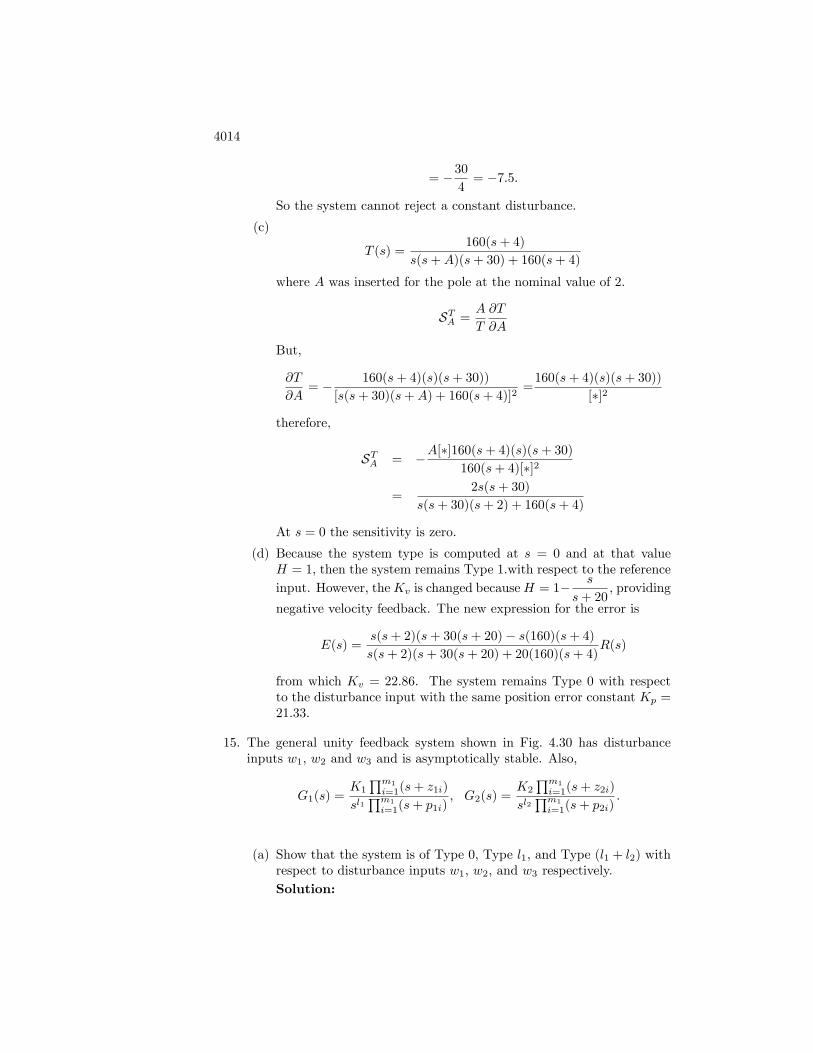
4014
= �304= �7:5:
So the system cannot reject a constant disturbance.
(c)
T (s) =160(s+ 4)
s(s+A)(s+ 30) + 160(s+ 4)
where A was inserted for the pole at the nominal value of 2.
STA =A
T
@T
@A
But,
@T
@A= � 160(s+ 4)(s)(s+ 30))
[s(s+ 30)(s+A) + 160(s+ 4)]2=160(s+ 4)(s)(s+ 30))
[�]2
therefore,
STA = �A[�]160(s+ 4)(s)(s+ 30)160(s+ 4)[�]2
=2s(s+ 30)
s(s+ 30)(s+ 2) + 160(s+ 4)
At s = 0 the sensitivity is zero.
(d) Because the system type is computed at s = 0 and at that valueH = 1; then the system remains Type 1.with respect to the referenceinput. However, theKv is changed becauseH = 1� s
s+ 20, providing
negative velocity feedback. The new expression for the error is
E(s) =s(s+ 2)(s+ 30(s+ 20)� s(160)(s+ 4)s(s+ 2)(s+ 30(s+ 20) + 20(160)(s+ 4)
R(s)
from which Kv = 22:86: The system remains Type 0 with respectto the disturbance input with the same position error constant Kp =21:33:
15. The general unity feedback system shown in Fig. 4.30 has disturbanceinputs w1, w2 and w3 and is asymptotically stable. Also,
G1(s) =K1
Qm1
i=1(s+ z1i)
sl1Qm1
i=1(s+ p1i); G2(s) =
K2
Qm1
i=1(s+ z2i)
sl2Qm1
i=1(s+ p2i):
(a) Show that the system is of Type 0, Type l1, and Type (l1 + l2) withrespect to disturbance inputs w1, w2, and w3 respectively.Solution:

4015
Figure 4.30: Single input-single output unity feedback system with disturbanceinputs
(a)
Y (s) =G1(s)G2(s)
1 +G1(s)G2(s)W1(s) =
K1K2[Qi(s+ zi)]W1(s)
sl1+l2Qi(s+ pi) +K1K2
Qi(s+ zi)
(i)
(pi; zi are the poles and zeros of G1 ; G2 not at the origin).
�ess = yss = lims!0
[sY (s)] = lims!0
[sW1(s)] Type 0
Y (s) =G2(s)
1 +G1(s)G2(s)W2(s) =
K2[Qi(s+ z2i)]s
l1Qi(s+ p1i)
�(s)W2(s) (ii)
�(s) is the characteristic polynomial, same as in (i) (denominator in(i)).
yss = [lims!0
s:W2(s):sl1 ]
Qi p1iQi z1i
Type `1
Y (s) =W3(s)
1 +G1(s)G2(s)=sl1+l2
Qi(s+ pi)
�(s)W3(s) (iii)
yss = [lims!0
s:W3(s):sl1+l2 ]
Qi piQi zi
Type `1 + `2
Y1 =1
s2 + s+ 1R1 +
s
s2 + s+ 1W1 +
s(s+ 1)
s2 + s+ 1W2
For constant disturbances, R1 = 0; W1(s) =W10
s; W2(s) =
W20
s
Y1 =W10 + (s+ 1)W20
s2 + s+ 1
Let u2 be the signal coupling systems 1 and 2:
U2 =(s+ 1)(R1 �W2) + s(s+ 1)W1
s2 + s+ 1
Y2 =R2
s2 + 3s+ 2+(s+ 1)U2s2 + 3s+ 2
=(s+ 1)2(�W2) + s(s+ 1)
2W2
(s2 + 3s+ 2)(s2 + s+ 1)

4016
Figure 4.31: System using integral control
The system Type w.r.t. disturbances:
y1 w:r:t: W1 Type 1
y1 w:r:t: W2 Type 1
y2 w:r:t: W1 Type 1
y2 w:r:t: W2 Type 0
can be determined by applying FVT to Y1 and Y2 or by inspection follow-ing the rule of part (a).
16. One possible representation of an automobile speed-control system withintegral control is shown in Fig. 4.31.
(a) With a zero reference velocity input (vc = 0), �nd the transfer func-tion relating the output speed v to the wind disturbance w.
(b) What is the steady-state response of v if w is a unit ramp function?
(c) What type is this system in relation to reference inputs? What is thevalue of the corresponding error constant?
(d) What is the type and corresponding error constant of this system inrelation to tracking the disturbance w?Solution:
(a)V (s)
W (s)=
ms
s2 +mk3s+mk1k2
(b)
vss = lims!0
sV (s)
W (s)
W0
s2=W0
k1k2
where W (s) =W0
s2:

4017
Figure 4.32: Control system for Problem 17
(c)
E = Vc � V = [1�
k1k2m
s(s+mk3)
1 +k1k2m
s(s+mk3)
]Vc =1
1 +mk1k2
s(s+mk3)| {z }G(s)
Vc
ess = lims!0
sVc1 +G(s)
Kp = lims!0
G(s) =1 =) e1(step input) = 0
Kv = lims!0
sG(s) =k1k2k3
=) e1(ramp input) =1
Kv=
k3k1k2
System is Type 1.
(d) For disturbances: If the disturbance is a ramp, the result of part (a)
shows that the steady state error, which is V; will be ess =1
k1k2:
Therefore, the system is Type 1 and the velocity constant is Kv =k1k2:
17. For the feedback system shown in Fig. 4.32, �nd the value of � that willmake the system Type 1 for K = 5. Give the corresponding velocityconstant. Show that the system is not robust by using this value of � andcomputing the tracking error e = r � y to a step reference for K = 4 andK = 6.
Solution:
Y =�KR
s+ 2 +KE = R�Y = s+ 2 +K(1� �)
s+ 2 +KRjK=5 =
s+ 7� 5�s+ 7
R
For � =7
5we have:
E =s
s+ 7R
ess(step input) = lims!0
ss
s+ 7
r0s= 0

4018
Figure 4.33: Control system for Problem 18
ess(ramp input) = lims!0
ss
s+ 7
v0s2=v07
So the system is Type 1.The system is not robust:
ess(step)jK=4 = lims!0
ss+ 2 + 4(�25 )
s+ 6
r0s=�r015
ess(step)jK=6 =�r020
So the system is Type 0 if K 6= 5:
18. Suppose you are given the system depicted in Fig. 4.33(a), where the plantparameter a is subject to variations.
(a) Find G(s) so that the system shown in Fig. 4.33(b) has the sametransfer function from r to y as the system in Fig. 4.33(a).
(b) Assume that a = 1 is the nominal value of the plant parameter.What is the system type and the error constant in this case?
(c) Now assume that a = 1 + �a, where �a is some perturbation to theplant parameter. What is the system type and the error constant forthe perturbed system?
Solution:
(a)
Y (s) =1
s(1 +
1
s+ a)U(s)
=1
s(1 +
1
s+ a)4(R(s)� Y (s) + 1
4(s+ a)U(s)) (1)

4019
U(s) = 4R(s)� 4Y (s) + 1
s+ aU(s)
(1� 1
s+ a)U(s) = 4R(s)� 4Y (s)
U(s) =4(s+ a)
s+ a� 1 [R(s)� Y (s)] (2)
Combining Eqs. (1) and (2) gives
Y (s) =1
s(s+ a+ 1
s+ a)(4(s+ a)
s+ a� 1)(R(s)� Y (s))
=4(s+ a� 1)s(s+ a� 1) [R(s)� Y (s)]
which means
G(s) =4(s+ a+ 1)
s(s+ a� 1)
(b) a = 1 therefore G(s) =4(s+ 2)
s2
E(s)
R(s)=
1
1 +G(s)=
s2
s2 + 4s+ 8
roots are in LHP so we can use the FVT,
ess;step = lim!0s(1
s)
s2
s2 + 4s+ 8= 0
therefore Kp =1
ess;ramp = lims!0
s(1
s2)
s2
s2 + 4s+ 8= 0
and Kv =1. The error to acceleration is
ess;parabola = lim!0s(1
s3)
s2
s2 + 4s+ 8=1
8
therefore Ka =18 and the system is Type 2
(c)E(s)
R(s)=
s(s+ �a)
s2 + (4 + �a)s+ 4(2 + �a)
for small �a, roots remain in LHP.
ess;step = lims!0
s(1
s)
s(s+ �a)
s2 + (4 + �a)s+ 4(2 + �a)= 0

4020
Figure 4.34: Two feedback systems for Problem 19
therefore Kp =1.
ess;ramp = lims!0
s(1
s2)
s(s+ �a)
s2 + (4 + �a)s+ 4(2 + �a)=
�a
4(2 + �a):
Therefore,Kv =4(2 + �a)
�a: For parabolic input, e(t)!1, therefore;Ka =
0: The system is now Type 1. Plant error (parameter variation)caused the change in system type.
19. Two feedback systems are shown in Fig. 4.34.
(a) Determine values for K1, K2, and K3 so that both systems:
i. exhibit zero steady-state error to step inputs (that is, both areType 1), and
ii. whose static velocity error constant Kv = 1 when K0 = 1.
(b) Suppose K0 undergoes a small perturbation: K0 ! K0+�K0. Whate¤ect does this have on the system type in each case? Which systemhas a type which is robust? Which system do you think would bepreferred?
Solution:
(a) System (a):
E = R� Y = R(s)
1 +G(s)
E(s) =s(4s+ 1)
4s2 + s+K0K1R(s)
Applying FTV:
ess;ramp =1
K1=
1
Kv=) K1 = Kv = 1
System (b):

4021
E = R� Y = 1 +G�K2G
1 +GR
E(s) =4s+ 1 +K3K0(1�K2)
4s+ 1 +K3K0R(s)
Applying FVT:
ess;step =1 +K3K0(1�K2)
1 +K3K0= 0
for K0 = 1 =) 1 +K3(1�K2) = 0
ess;ramp =4
1 +K3=
1
Kv
for Kv = 1 =) K3 = 3
=) K2 =4
3; K3 = 3
(b) Let K0 = K0 + �K0 In System (a):
ess;step = lims!0
ss(4s+ 1)
(4s2 + s+K0 + �K0)
1
s= 0
regardless of K0 value. In System (b):
ess;step =1 +K3(K0 + �K0)(1�K2)
1 +K3(K0 + �K0)jK0=1 =
��K0
1 + 3(1 + �K06= 0
Thus the system type of System (b) is not robust (it is a �calibrated�system type.) Control engineers prefer system (a) over (b) becauseit is more robust to parameter changes. (This can be expected fora closed-loop with feedback to the input while (b) has an open-loopstage to entering the feedback loop.)
20. You are given the system shown in Fig. 4.35, where the feedback gain �is subject to variations. You are to design a controller for this system sothat the output y(t) accurately tracks the reference input r(t).
(a) Let � = 1. You are given the following three options for the controllerDi(s):
D1(s) = kp; D2(s) =kps+ kI
s; D3(s) =
kps2 + kIs+ k2s2
:
Choose the controller (including particular values for the controllerconstants) that will result in a Type 1 system with a steady-stateerror to a unit reference ramp of less than 1
10 .

4022
Figure 4.35: Control system for Problem 20
(b) Next, suppose that there is some attenuation in the feedback paththat is modeled by � = 0:9. Find the steady-state error due to aramp input for your choice of Di(s) in part (a).
(c) If � = 0:9, what is the system type for part (b)? What are the valuesof the appropriate error constant?Solution:
(a) Need an integrator in the loop - choose D2(s)
T (s) =Y (s)
R(s)=
10(kps+ kI)
s(s+ 1)(s+ 10)
1 + �10(kps+ kI)
s(s+ 1)(s+ 10)
E(s) = (1�T (s))R(s) = [s(s+ 1)(s+ 10) + 10(kps+ kI)� � 10(kps+ kI)s(s+ 1)(s+ 10) + 10(kps+ kI)�
]1
s2
For � = 1,
ess = lims!0
s[s(s+ 1)(s+ 10)
s(s+ 1)(s+ 10) + 10(kps+ kI)]1
s2
=10
10kI=1
kITherefore kI � 10 will meet the steady-state speci�cations Theclosed-loop poles are the roots of s3+11s2+10s+10(kps+ kI) = 0.The Routh�s array is,
s3 : 1 10(1 + kp)s2 : 11 10kI
s1 :110(1+kp)�10kI
11s0 : 10kI
which requires kI > 0 and 11(1 + kp)� kI > 0 for stability.(b) From above, with � = 0:9
E(s) = [s(s+ 1)(s+ 10) + 9(kps+ kI)� 10(kps+ kI)
s(s+ 1)(s+ 10) + 9(kps+ kI)]R(s)
=s(s+ 1)(s+ 10)� kp�kI
s(s+ 1)(s+ 10) + 9(kps+ kI)R(s)

4023
Figure 4.36: Control system for Problem 21
If kp and kI are chosen so that the system is stable, applying the
FVT for R(s) =1
s2results in ess ! 1: The system is no longer
Type 1.
(c) Try R(s) =1
s
lims!0
sE(s) = lims!0
s(s+ 1)(s+ 10)� kps�kIs(s+ 1)(s+ 10) + 9(kps+ kI)
= � kI9kI
= �19
and the system is Type 0. Kp is de�ned such that jessj =1
1 +Kp.
Thus, Kp = 8: Without the magnitude an equivalent result is thatKp = �10:
21. Consider the system shown in Fig. 4.36.
(a) Find the transfer function from the reference input to the trackingerror.
(b) For this system to respond to inputs of the form r(t) = tn1(t) (wheren < q) with zero steady-state error, what constraint is placed on theopen-loop poles p1; p2; � � � ; pq?Solution:
(a)E(s)
R(s)=
1
1 +G(s)=
Qqi=1(s+ pi)Qq
i=1(s+ pi) + 1
(b)
r(t) = tn =) R(s) =n!
sn+1
ess = lims!0
sn!
sn+1
Qqi=1(s+ pi)Qq
i=1(s+ pi) + 1
If ess is to be zero the system must have at least n + 1 poles at

4024
the origin:
ess = lims!0
sn!
sn+1sn+1
Qqi=1(s+ pi)
sn+1Qqi=1(s+ pi) + 1
= 0
22. A linear ODE model of the DC motor with negligible armature inductance(La = 0) and with a disturbance torque w was given earlier in the chapter;it is restated here, in slightly di¤erent form, as
JRaKt
��m +Ke_�m = �a +
RaKtw;
where �m is measured in radians. Dividing through by the coe¢ cient of��m, we obtain
��m + a1 _�m = b0�a + c0w;
where
a1 =KtKe
JRa; b0 =
Kt
JRa; c0 =
1
J:
With rotating potentiometers, it is possible to measure the positioningerror between � and the reference angle �r or e = �ref � �m. With atachometer we can measure the motor speed _�m. Consider using feedbackof the error e and the motor speed _�m in the form
�a = K(e� TD _�m);
where K and TD are controller gains to be determined.
(a) Draw a block diagram of the resulting feedback system showing both�m and _�m as variables in the diagram representing the motor.
(b) Suppose the numbers work out so that a1 = 65, b0 = 200, andc0 = 10. If there is no load torque (w = 0), what speed (in rpm)results from va = 100 V?
(c) Using the parameter values given in part (b), let the control be D =kp + kDs and �nd kp and kD so that, using the results of Chapter3, a step change in �ref with zero load torque results in a transientthat has an approximately 17% overshoot and that settles to within5% of steady-state in less than 0:05 sec.
(d) Derive an expression for the steady-state error to a reference angleinput, and compute its value for your design in part (c) assuming�ref = 1 rad.
(e) Derive an expression for the steady-state error to a constant distur-bance torque when �ref = 0, and compute its value for your designin part (c) assuming w = 1:0.Solution:
(a) Block diagram:

4025
Block diagram for Problem 4.22
(b) If Va=constant the system is in steady state:
_� =b0a1Va =
200� 10065
60
2�
rad:sec�1
rpm= 2938 rpm
(c)�
�r=
Kb0s2 + s(a1 + TDKb0) +Kb0
=!2n
s2 + 2�!ns+ !2n
Mp = 17%; =): � = 0:5 ts = 0:05 sec. to 5% :
=) e��!nts = 0:05 =) �!n = 60 =) !n = 120
Comparing coe¢ cients:
K = 72 ; TD = 3:8� 10�3
(d) Steady-state error:
E(s) = �r � � =s(s+ a1 + TDKb0)
s2 + s(a1 + TDKb0) +Kb0�r
For �r =1
s:
ess = lims!0
sE(s) = 0 (Type 1)
(e) Response to torque:
�
QL=
c0s2 + s(a1 + TDKb0) +Kb0
�ss = lims!0
s:�(s) = lims!0
sc0
s2 + : : :
1
s=
c0Kb0
=1
1440rad

4026
23. We wish to design an automatic speed control for an automobile. Assumethat (1) the car has a mass m of 1000 kg, (2) the accelerator is the controlU and supplies a force on the automobile of 10 N per degree of acceleratormotion, and (3) air drag provides a friction force proportional to velocityof 10 N � sec=m.
(a) Obtain the transfer function from control input U to the velocity ofthe automobile.
(b) Assume the velocity changes are given by
V (s) =1
s+ 0:02U(s) +
0:05
s+ 0:02W (s);
where V is given in meters per second, U is in degrees, and W isthe percent grade of the road. Design a proportional control lawU = �kpV that will maintain a velocity error of less than 1 m/sec inthe presence of a constant 2% grade.
(c) Discuss what advantage (if any) integral control would have for thisproblem.
(d) Assuming that pure integral control (that is, no proportional term) isadvantageous, select the feedback gain so that the roots have criticaldamping (� = 1).Solution:a.
m�x =X
F = Kau�D _xLfm _v = Kau�Dvg
V
U=
Ka
ms+D=
0:01
s+ 0:01
b. Error:
E(s) = Vd � V = Vd �
kps+ 0:02
1 +kp
s+ 0:02
Vd +0:05
1
s+ 0:02
1 +kp
s+ 0:02
G(s)
=(s+ 0:02)Vd � 0:05G
s+ 0:02 + kp
If we want error < 1 m/sec in presence of grade, we in fact needjess(step)j < 1. Assume no input : (Vd = 0)
ess(step) = lims!0
s(�0:05
s+ 0:02 + kp)2
s=
�0:10:02 + kp
j �0:10:02 + kp
j < 1

4027
Figure 4.37: Automobile speed-control system
While solving the inequality apply (or check) restriction that polesare in LHP.
=) kp > 0:08
c. The obvious advantage of integral control would be zero s.s. errorfor step input (Type 1 system would result).
d. Pure integral control: kp !kIs
E(s) =s(s+ 0:02)Vd � 0:05sG(s)
s2 + 0:02s+ kI
� = 1 =) !n = 0:01 =) kI = 0:0001
24. Consider the automobile speed control system depicted in Fig. 4.37.
(a) Find the transfer functions from W (s) and from R(s) to Y (s).
(b) Assume that the desired speed is a constant reference r, so thatR(s) = ro=s. Assume that the road is level, so w(t) = 0. Computevalues of the gains K, Hr, and Hf to guarantee that
limt!1
y(t) = ro:
Include both the open-loop (assuming Hy = 0) and feedback cases(Hy 6= 0) in your discussion.
(c) Repeat part (b) assuming that a constant grade disturbance W (s) =wo=s is present in addition to the reference input. In particular,�nd the variation in speed due to the grade change for both thefeed forward and feedback cases. Use your results to explain (1) whyfeedback control is necessary and (2) how the gain kp should be chosento reduce steady-state error.

4028
(d) Assume that w(t) = 0 and that the gain A undergoes the perturba-tion A + �A. Determine the error in speed due to the gain changefor both the feed forward and feedback cases. How should the gainsbe chosen in this case to reduce the e¤ects of �A?Solution:
(a)
Y (s) =B
s+ a+ kpAHyW (s) +
kpAHrs+ a+ kpAHy
R(s)
(b) Feedforward:(Hy = 0)
lims!0
sY (s) = lims!0
kpAHrs+ a+ 0
r = r
therefore,kp =
a
AHr:
Feedback:limt!1
y(t) = r
results inkpAHr
a+ kpAHyr = r
Choose kp for performance and Hy for sensor characteristics, and set
Hr =a+AkpHy
kpA
(c) Feedforward:
limt!1
y(t) =Bw
a+ar
a
= r +Bw
aTherefore,
�yff (1) =Bw
a;
all quantities are �xed- no way to reduce e¤ect of disturbance.Feedback:
limt!1
y(t) =B
a+ kpAHyw +
kpAHra+ kpAHy
r
=B
a+ kpAHyw + r
(if Hr is chosen as in part (b)). Therefore,
�yfb(1) =B
a+ kpAHyw
E¤ect of disturbance can be made small by choosing kp large.

4029
(d) Feedforward: using kp =a
AHras derived in part (b),
yff (1) = (1 +�A
A)r
therefore,
�yff (1) =�A
Ar
or�yff (1)
r=�A
A
which means that 5% error in A results in 5% error in tracking.Feedback:
yfb(1) =(A+ �A)kpHr
a+ (A+ �A)kpHyr
using value for Hr chosen in part (b) gives
yfb(1) = [(A+ �A)
a+ (A+ �A)kpHy
a+ kpAHyA
]r
= r +a�A
aA+ (A+ �A)kpAHyr
�= r +a
a+ kpAHy
�A
A
�yfb(1)r
=a
a+ kpAHy
�A
A
Tracking error due to parameter variation can be reduced by choosingkp large.
25. Consider the multivariable system shown in Fig. 4.38. Assume that thesystem is stable. Find the transfer functions from each disturbance inputto each output and determine the steady-state values of y1 and y2 forconstant disturbances. We de�ne a multivariable system to be Type kwith respect to polynomial inputs at wi if the steady-state value of everyoutput is zero for any combination of inputs of degree less than k and atleast one input is a non-zero constant for an input of degree k: What isthe system type with respect to disturbance rejection at w1? At w2?
Solution:
(a)
Y1 =1
s2 + s+ 1R1 +
s
s2 + s+ 1W1 +
s(s+ 1)
s2 + s+ 1W2
For constant disturbances, R1 = 0; W1(s) =W10
s; W2(s) =
W20
s
Y1 =W10 + (s+ 1)W20
s2 + s+ 1

4030
Figure 4.38: Multivariable system
Let u2 be the signal coupling systems 1 and 2:
U2 =(s+ 1)(R1 �W2) + s(s+ 1)W1
s2 + s+ 1
Y2 =R2
s2 + 3s+ 2+(s+ 1)U2s2 + 3s+ 2
=(s+ 1)2(�W2) + s(s+ 1)
2W2
(s2 + 3s+ 2)(s2 + s+ 1)
The system type w.r.t. disturbances:
y1 w:r:t: W1 Type 1
y1 w:r:t: W2 Type 1
y2 w:r:t: W1 Type 1
y2 w:r:t: W2 Type 0
can be determined by applying FVT to Y1 and Y2 or by inspection.
Problems and Solutions for Section 4.3: The Three Term con-troller: PID control
26. The transfer functions of speed control for a magnetic tape-drive systemare shown in Fig. 4.39. The speed sensor is fast enough that its dynamicscan be neglected and the diagram shows the equivalent unity feedbacksystem.
(a) Assuming the reference is zero, what is the steady-state error due toa step disturbance torque of 1 N �m? What must the ampli�er gainK be in order to make the steady-state error ess � 0:001 rad/sec.?
(b) Plot the roots of the closed-loop system in the complex plane, andaccurately sketch the time response of the output for a step referenceinput using the gain K computed in part (a).

4031
Figure 4.39: Speed-control system for a magnetic tape drive
(c) Plot the region in the complex plane of acceptable closed-loop polescorresponding to the speci�cations of a 1% settling time of ts �0:1 sec. and an overshoot Mp � 5%.
(d) Give values for kp and kD for a PD controller which will meet thespeci�cations.
(e) How would the disturbance-induced steady-state error change withthe new control scheme in part (d)? How could the steady-state errorto a disturbance torque be eliminated entirely?
Solution:
(a) TF for disturbance:
Y
W=
1
Js+ b
1 +1
Js+ b:10kp0:5s+ 1
b = 1 ; J = 0:1
ess(step in W) = lims!0
s1
s
Y
W=
1
1 + 10kp
ess � 0:01 ; kp � 9:9 pick kp = 10:
(b)
Y (s)
r(s)=
10kp0:5s+ 1
:1
Js+ b
1 +1
Js+ b:10kp0:5s+ 1
=2000
s2 + 12s+ 2020
!n =p2020 ' 45 ; � = 12
2p2020
�= 0:13
The roots are undesirable (damping too low, high overshoot).

4032
50 40 30 20 10 050
40
30
20
10
0
10
20
30
40
50Lines of damping and wn
*
*0 0.5 1
0
0.2
0.4
0.6
0.8
1
1.2
1.4
1.6
1.8step response
Time (sec)
Am
plitu
de
(c) For ts � 0:1 =) � � 46 For Mp � 0:05 =) � � 0:7
160 140 120 100 80 60 40 20 060
40
20
0
20
40
60Lines of damping and wn
s-plane for part(c)
(a) d. We know that larger !n and � are needed. This can be achievedby increasing kp and adding derivative feedback as in Fig. 4.12 (
Y (s)
r(s)=
10kp0:5s+ 1
:1
Js+ b
1 +10kp(kDs+ 1)
(0:5s+ 1)(Js+ b)
=200kp
s2 + (12 + 200kp:kD)s+ 20(1 + 10kp)
By choosing kp and kD any � and !n may be achieved.e. The TF to disturbance with new control:
Y
W=
1
Js+ b
1 +1
Js+ b:10kp(kDs+ 1)
(0:5s+ 1)
=20(0:5s+ 1)
s2 + (12 + 200kpkD)s+ 20(1 + 10kp)
ess(step in W) =1
1 + 10kp

4033
Figure 4.40: Control system for Problem 27
As before derivative feedback a¤ects transient response only. To elim-inate steady-state error we can add an integrator to the loop. This
can be represented by replacing kp with kp +kIsin the forward loop
and still keeping PD control in the feedback loop to obtain
Y
W=
20(0:5s+ 1)s
s3 + (12 + 200kpkD)s2 + (20 + 200kp + 200kIkD)s+ 200kI
ess(step in W) = 0:
27. Consider the system shown in Fig. 4.40 with PI control.
(a) Determine the transfer function from R to Y .
(b) Determine the transfer function from W to Y .
(c) What is the system type and error constant with respect to referencetracking?
(d) What is the system type and error constant with respect to distur-bance rejection?Solution:
(a)Y (s)
R(s)=
10(kI + kps)
s[s(s+ 1) + 20] + 10(kI + kps):
(b)Y (s)
W (s)=
10s
s[s(s+ 1) + 20] + 10(kI + kps):
(c) The characteristic equation is s3+ s2+(10kp+20)s+10kI = 0. TheRouth�s array is
s3 : 1 10kp + 20s2 : 1 10kIs1 : 10kp + 20� 10kIs0 : 10kI
For stability we must have kI > 0 and kp > kI � 2.

4034
(d) System is Type 1 with respect to both r and w. The velocity constantwith respect to reference tracking is Kv = kI=2 and with respect todisturbance rejection is kI :
28. Consider the second-order plant with transfer function
G(s) =1
(s+ 1)(5s+ 1):
and in a unity feedback structure.
(a) Determine the system type and error constant with respect to track-ing polynomial reference inputs of the system for P [D = kp], PD
[D = kp + kDs], and PID [D = kp +kIs+ kDs] controllers. Let
kp = 19, kI = 0:5, and kD =4
19:
(b) Determine the system type and error constant of the system withrespect to disturbance inputs for each of the three regulators in part(a) with respect to rejecting polynomial disturbances w(t) at theinput to the plant.
(c) Is this system better at tracking references or rejecting disturbances?Explain your response brie�y.
(d) Verify your results for parts (a) and (b) using Matlab by plot-ting unit step and ramp responses for both tracking and disturbancerejection.
Solution:
a. This plant has no pole at the origin and DC gain of 1 so, unlessthe controller has such a pole, the system will be Type 0.
Thus, we have: P and PD are Type 0, Kp = kp = 19;PID is Type 1,Kv = kI = 0:5
b. Again, P and PD are Type 0, Kp = kp = 19;PID is Type 1,Kv = kI = 0:5:
c. Because the Types and error constants are the same, this systemdoes the same with references as with disturbances.
d. We expect the steady state error to steps to be 0 and to unitramps to be 1=kp = 1=0:5 = 2:0: Note that steady-state is after along time!

4035
0 10 20 30 40 50 60 70 80 90 1000.1
0.05
0
0.05
0.1
0.15Error to a reference s tep
Error to a reference step.0 10 20 30 40 50 60 70 80 90 100
0
0.2
0.4
0.6
0.8
1
1.2
1.4
1.6
1.8
2Error response to a reference ramp
Error to a reference ramp
Notice that these transients are very slow. They are the consequenceof a pole at s = �0:0252: A good rule of thumb is that a tran-sient is over in 5 time constants. In this case the time constantis 1=0:0252 = 39:68: Therefore we�d expect the transient to go onfor about 200 seconds! The responses to disturbances are similar:.
.
0 10 20 30 40 50 60 70 80 90 1000.07
0.06
0.05
0.04
0.03
0.02
0.01
0E rror for a disturbance step
Error to a disturbance step0 10 20 30 40 50 60 70 80 90 100
2
1.8
1.6
1.4
1.2
1
0.8
0.6
0.4
0.2
0
Error to a disturbance ramp.In
this case, the disturbance ramp does not excite the fast roots verymuch at all.
29. The DC-motor speed control shown in Fig. 4.41 is described by the dif-ferential equation
_y + 60y = 600va � 1500w;where y is the motor speed, va is the armature voltage, and w is the loadtorque. Assume the armature voltage is computed using the PI control law
va = ��kpe+ kI
Z t
0
edt
�:
where e = r � y:

4036
Figure 4.41: D.C. Motor speed control block diagram for Problems 29 and 30
(a) Compute the transfer function from W to Y as a function of kp andkI .
(b) Compute values for kp and kI so that the characteristic equation ofthe closed-loop system will have roots at �60� 60j.Solution:
(a) Transfer function: Set R = 0; then E = �Y
(s+ 60)Y (s) = �600[kpY (s) +kIsY (s)]� 1500W (s)
Y (s)
W (s)=
�1500ss2 + 60(1 + 10kp)s+ 600kI
(b) For roots at �60� j60 : comparing to the standard form:
s2 + 2�!ns+ !2n = 0 =) s = ��!n � j!n
q1� �2
!n = 60p2 ; � = 0:707
600kI = (60p2)2 =) kI = 12
60(1 + 10kp) = 2� 0:707� 60p2 =) kp = 0:1
30. For the system in Problem 29, compute the following steady-state errors:
(a) to a unit-step reference input;
(b) to a unit-ramp reference input;
(c) to a unit-step disturbance input;
(d) for a unit-ramp disturbance input.
(e) Verify your answers to (a) and (d) usingMatlab. Note that a rampresponse can be generated as a step response of a system modi�edby an added integrator at the reference input.

4037
Solution:a. From Problem 21, kp = 0:1 and kI = 12: The DC gain of the plantis 10 so the Kv = 10kI : The system is Type 1 so the error to a stepis 0.
b. To a unit ramp, the error is1
Kv=
1
10kI=
1
120:
c. For a disturbance input, the system is also Type 1. The error toa step will be 0.d. For a unit ramp disturbance input the error equals the output andis given by
E = � 1500
s+ 60 + 600DW
= � 1500s
s2 + 60s+ 600(kP s+ kI)W
ess = � 524
for W = 1=s2
e.
0 0.02 0.04 0.06 0.08 0.1 0.12 0.14 0.16 0.18 0.20.2
0
0.2
0.4
0.6
0.8
1
1.2E rror response to a reference step
Error Response to a ReferenceStep
0 0.02 0.04 0.06 0.08 0.1 0.12 0.14 0.16 0.18 0.20
0.002
0.004
0.006
0.008
0.01
0.012E rror response to a reference ramp
Error Response to a ReferenceRamp
Asthese �gures show, the error to a step goes to zero and that to a rampgoes to 1=kI = 1=120:
0 0.02 0.04 0.06 0.08 0.1 0.12 0.14 0.16 0.18 0.28
7
6
5
4
3
2
1
0
1Error response to a disturbance step
Error to a Disturbance Step0 0.02 0.04 0.06 0.08 0.1 0.12 0.14 0.16 0.18 0.2
0.25
0.2
0.15
0.1
0.05
0Error response to a disturbance ramp
Error to a Disturbance Ramp

4038
Figure 4.42: Satellite attitude control
And in this case, the error to a disturbance step goes to zero and theerror to a disturbance ramp goes to ess = 1=kI = �0:208:
31. Consider the satellite-attitude control problem shown in Fig. 4.42 wherethe normalized parameters are
J = 10 spacecraft inertia; N-m-sec2=rad
�r = reference satellite attitude; rad.
� = actual satellite attitude; rad.
Hy = 1 sensor scale; factor volts/rad.
Hr = 1 reference sensor scale factor; volts/rad.
w = disturbance torque: N-m
(a) Use proportional control, P, with D(s) = kp, and give the range ofvalues for kp for which the system will be stable.
(b) Use PD control and let D(s) = (kp+kDs) and determine the systemtype and error constant with respect to reference inputs.
(c) Use PD control, let D(s) = (kp + kDs) and determine the systemtype and error constant with respect to disturbance inputs.
(d) Use PI control, let D(s) = (kp + kI=s), and determine the systemtype and error constant with respect to reference inputs.
(e) Use PI control, let D(s) = (kp + kI=s), and determine the systemtype and error constant with respect to disturbance inputs.
(f) Use PID control, let D(s) = (kp + kI=s + kDs) and determine thesystem type and error constant with respect to reference inputs.
(g) Use PID control, let D(s) = (kp + kI=s + kDs) and determine thesystem type and error constant with respect to disturbance inputs.
Solution:
(a) D(s) = kp; The characteristic equation is
1 +HyD(s)1
Js2= 0

4039
Js2 +Hykp = 0
or s = �jrHykpJ
so that no additional damping is provided. The
system cannot be made stable with proportional control alone.
(b) Steady-state error to reference steps.
�(s)
�r(s)= Hr
D(s)1
Js2
1 +D(s)Hy1
Js2
= Hr(kp + kDs)
Js2 + (kp + kDs)Hy
The parameters can be selected to make the (closed-loop) system
stable. If �r(s) =1
sthen using the FVT (assuming the system is
stable)
�ss =HrHy
and there is zero steady-state error if Hr = Hy (i.e., unity feedback).
(c) Steady-state error to disturbance steps
�(s)
W (s)=
1
Js2 + (kp + kDs)Hy
If W (s) =1
sthen using the FVT (assuming system is stable), the
error is �ss = �1
kpHy.
(d) The characteristic equation is
1 +HyD(s)1
Js2= 0
With PI control,Js3 +Hykps+HykI = 0
From the Hurwitz�s test, with the s2 term missing the system willalways have (at least) one pole not in the LHP. Hence, this is not agood control strategy.
(e) See d above.
(f) The characteristic equation with PID control is
1 +Hy(kp +kIs+ kDs)
1
Js2= 0
orJs3 +HykDs
2 +Hykps+HykI = 0

4040
There is now control over all the three poles and the system can bemade stable.
�(s)
�r(s)= Hr
D(s)1
Js2
1 +D(s)Hy1
Js2
=Hr(kp+
kIs+ kDs)
Js2 + (kp+kIs+ kDs)Hy
=Hr(kDs
2 + kps+ kI)
Js3 + (kDs2 + kps+ kI)Hy
If �r(s) =1
sthen using the FVT (assuming system is stable)
�ss =HrHy
and there is zero steady-state error if Hr = Hy (i.e., unity feedback).In that case, the system is Type 3 and the (Jerk!) error constant is
KJ =kIJ:
(g) The error to a disturbance is found from
�(s)
W (s)=
s
Js3 +Hy(kDs2 + kps+ kI)
If W (s) =1
sthen using the FVT (assuming the system is stable),
�ss = 0; the system is Type 1 and the error constant is Kv = Hykp:
32. The unit-step response of a paper machine is shown in Fig. 4.43(a) wherethe input into the system is stock �ow onto the wire and the output is basisweight (thickness). The time delay and slope of the transient response maybe determined from the �gure.
(a) Find the proportional, PI, and PID-controller parameters using theZeigler�Nichols transient-response method.
(b) Using proportional feedback control, control designers have obtaineda closed-loop system with the unit impulse response shown in Fig. 4.43(b).When the gain Ku = 8:556, the system is on the verge of instabil-ity. Determine the proportional-, PI-, and PID-controller parametersaccording to the Zeigler�Nichols ultimate sensitivity method.Solution:
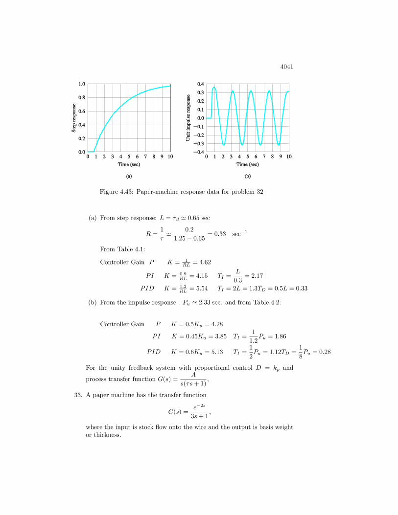
4041
Figure 4.43: Paper-machine response data for problem 32
(a) From step response: L = �d ' 0:65 sec
R =1
�' 0:2
1:25� 0:65 = 0:33 sec�1
From Table 4.1:
Controller Gain P K = 1RL = 4:62
PI K = 0:9RL = 4:15 TI =
L
0:3= 2:17
PID K = 1:2RL = 5:54 TI = 2L = 1:3TD = 0:5L = 0:33
(b) From the impulse response: Pu ' 2:33 sec. and from Table 4.2:
Controller Gain P K = 0:5Ku = 4:28
PI K = 0:45Ku = 3:85 TI =1
1:2Pu = 1:86
PID K = 0:6Ku = 5:13 TI =1
2Pu = 1:12TD =
1
8Pu = 0:28
For the unity feedback system with proportional control D = kp and
process transfer function G(s) =A
s(�s+ 1);
33. A paper machine has the transfer function
G(s) =e�2s
3s+ 1;
where the input is stock �ow onto the wire and the output is basis weightor thickness.

4042
Figure 4.44: Unit impulse response for paper-machine in Problem 33
(a) Find the PID-controller parameters using the Zeigler�Nichols tuningrules.
(b) The system becomes marginally stable for a proportional gain ofKu = 3:044 as shown by the unit impulse response in Fig. 4.44.Find the optimal PID-controller parameters according to the Zeigler�Nichols tuning rules.
Solution:
(a) From the transfer function: L = �d ' 2 sec
R =1
3' 0:33 sec�1
From Table 4.1:
Controller Gain P K =1
RL1:5
PI K = 0:9RL = 1:35 TI =
L
0:3= 6:66
PID K = 1:2RL = 1:8 TI = 2L = 4 TD = 0:5L = 1:0
(b) From the impulse response: Pu ' 7 sec From Table 4.2:
Controller Gain P K = 0:5Ku = 1:52
PI K = 0:45Ku = 1:37 TI =1
1:2Pu = 5:83
PID K = 0:6Ku = 1:82 TI =1
2Pu = 3:5TD =
1
8Pu = 0:875

4043
Problems and Solutions for Section 4.4: Introduction to DigitalControl
34. Compute the discrete equivalents for the following possible controllers us-ing the trapezoid rule of Eq. (4.98). Let Ts = 0:05 in each case.
(a) D1(s) = (s+ 2)=2,
(b) D2(s) = 2s+ 2
s+ 4,
(c) D3(s) = 5(s+ 2)
s+ 10,
(d) D4(s) = 5(s+ 2)(s+ 0:1)
(s+ 10)(s+ 0:01)
Solution:
(a) Using the formula s 2
Ts
z � 1z + 1
we �nd D1(z) =21z � 19z + 1
(b) D2(z) =1:909z � 1:727z � 0:8182
(c) D3(z) =4:2z � 3:8z � 0:6
(d) D4(z) =4:209z2 � 7:997z + 3:79z2 � 1:6z + 0:5997
35. Give the di¤erence equations corresponding to the discrete controllersfound in Problem 34 respectively
(a) part 1.
(b) part 2.
(c) part 3.
(d) part 4.
Solution:
(a) Reduce the z� transforms to be in terms of z�1 if you want the equa-tions in terms of past values. We have divided by the coe¢ cient of thehighest power if z in the denominator to get the coe¢ cient of u(k) to
be 1:0 in each case. For part (a),U
E=21z � 19z + 1
=21� 19z�11 + z�1
and
thus [1 + z�1]U(z) = [21 � 19z�1]E(z) from which, as z�1U(z) =)u(k � 1) we getu(k) = �u(k � 1) + 21e(k)� 19e(k � 1): We have suppressed the Tsin these equations. It should properly be u(kTs); u([k � 1]Ts); etc.
(b) u(k) = 0:8182u(k � 1) + 1:909e(k)� 1:727e(k � 1):(c) u(k) = 0:6u(k � 1) + 4:2e(k)� 3:8e(k � 1)

4044
(d) u(k) = 1:6u(k � 1) � 0:5997u(k � 2) + 4:209e(k) � 7:997e(k � 1) +3:79e(k � 2)

Chapter 5
The Root-Locus DesignMethod
Problems and solutions for Section 5.1
1. Set up the following characteristic equations in the form suited to Evans�sroot-locus method. Give L(s); a(s); and b(s) and the parameter, K; interms of the original parameters in each case. Be sure to select K so thata(s) and b(s) are monic in each case and the degree of b(s) is not greaterthan that of a(s):
(a) s+ (1=�) = 0 versus parameter �
(b) s2 + cs+ c+ 1 = 0 versus parameter c
(c) (s+ c)3 +A(Ts+ 1) = 0
i. versus parameter A,ii. versus parameter T ,iii. versus the parameter c, if possible. Say why you can or can not.
Can a plot of the roots be drawn versus c for given constantvalues of A and T by any means at all
(d) 1 + [kp +kIs+
kDs
�s+ 1]G(s) = 0: Assume that G(s) = A
c(s)
d(s)where
c(s) and d(s) are monic polynomials with the degree of d(s) greaterthan that of c(s).
i. versus kpii. versus kIiii. versus kDiv. versus �
5001

5002 CHAPTER 5. THE ROOT-LOCUS DESIGN METHOD
Solution:
(a) K = 1=� ; a = s; b = 1
(b) K = c; a = s2 + 1; b = s+ 1
(c) Part (c)
i. K = AT ; a = (s+ c)3; b = s+ 1=T
ii. K = AT ; a = (s+ c)3 +A; b = s
iii. The parameter c enters the equation in a nonlinear way and astandard root locus does not apply. However, using a polynomialsolver, the roots can be plotted versus c:
(d) Part (d)
i. K = kpA� ; a = s(s+ 1=�)d(s) + kI(s+ 1=�)c(s) +kD�s2Ac(s);
b = s(s+ 1=�)c(s)
ii. K = AkI ; a = s(s + 1=�)d(s) + Akps(s + 1=�) +kD�s2Ac(s);
b = s(s+ 1=�)c(s)
iii. K =AkD�; a = s(s + 1=�)d(s) + Akps(s + 1=�)c(s) + AkI(s +
1=�)c(s); b = s2c(s)
iv. K = 1=� ; a = s2d(s) + kpAs2c(s) + kIAsc(s); b = sd(s) +
kpsAc(s) + kIAc(s) + kDs2Ac(s)

5003
Problems and solutions for Section 5.2
2. Roughly sketch the root loci for the pole-zero maps as shown in Fig. 5.51.Show your estimates of the center and angles of the asymptotes, a roughevaluation of arrival and departure angles for complex poles and zeros,and the loci for positive values of the parameter K. Each pole-zero mapis from a characteristic equation of the form
1 +Kb(s)
a(s)= 0;
where the roots of the numerator b(s) are shown as small circles o and theroots of the denominator a(s) are shown as �0s on the s-plane. Note thatin Fig. 5.51(c), there are two poles at the origin and there are two poleson the imaginary axis in (f), slightly o¤ the real axis.
Solution:

5004 CHAPTER 5. THE ROOT-LOCUS DESIGN METHOD
10 5 0 52
1
0
1
2
Root loci f or Problem 5.2
Real Axis
Imag
inar
y Ax
is
6 4 2 0 22
1
0
1
2
Real Axis
Imag
inar
y Ax
is
4 2 0 22
1
0
1
2
Real Axis
Imag
inar
y Ax
is
4 2 0 21
0.5
0
0.5
1
Real Axis
Imag
inar
y Ax
is
10 5 0 510
5
0
5
10
Real Axis
Imag
inar
y Ax
is
4 2 0 2 44
2
0
2
4
Real Axis
Imag
inar
y Ax
is

5005
We had to make up some numbers to do it on Matlab, so the resultspartly depend on what was dreamed up, but the idea here is just get thebasic rules right.
(a)a(s) = s2 + s; b(s) = s+ 1
Breakin(s) -3.43; Breakaway(s) -0.586
(b) a(s) = s2 + 0:2s+ 1; b(s) = s+ 1
Angle of departure: 135.7
Breakin(s) -4.97
(c) a(s) = s2; b(s) = (s+ 1)
Breakin(s) -2
(d) a(s) = s2 + 5s+ 6; b(s) = s2 + s
Breakin(s) -2.37
Breakaway(s) -0.634
(e) a(s) = s3 + 3s2 + 4s� 8
Center of asymptotes -1
Angles of asymptotes �60; 180
Angle of departure: -56.3
(f) a(s) = s3 + 3s2 + s� 5; b(s) = s+ 1
Center of asymptotes -.667
Angles of asymptotes �60; �180
Angle of departure: -90
Breakin(s) -2.06
Breakaway(s) 0:503
But, to get this one right, all you have to do is get the real axis segmentsand the 4 asymptotes going out at the right angles. You don�t know,really, where it breaks away from the real axis nor where the center ofasymptotes are.

5006 CHAPTER 5. THE ROOT-LOCUS DESIGN METHOD
3. For the characteristic equation
1 +K
s(s+ 1)(s+ 5)= 0 :
(a) Draw the real-axis segments of the corresponding root locus.
(b) Sketch the asymptotes of the locus for K !1.
(c) For what value of K are the roots on the imaginary axis?
(d) Verify your sketch with a MATLAB plot.
Solution:
(a) The real axis segments are 0 > � > �1; �5 > �
(b) � = �6=3 = �2; �i = �60; 180
(c) Ko = 30
Roo t Loc us
Rea l Ax i s
Ima
g A
xis
15 10 5 0 5
10
5
0
5
10
Solution for Problem 5.3

5007
4. Real poles and zeros. Sketch the root locus with respect to K for theequation 1 + KL(s) = 0 and the following choices for L(s). Be sure togive the asymptotes, arrival and departure angles at any complex zero orpole, and the frequency of any imaginary-axis crossing. After completingeach hand sketch verify your results using MATLAB. Turn in your handsketches and the MATLAB results on the same scales.
(a) L(s) =(s+ 2)
s(s+ 1)(s+ 5)(s+ 10)
(b) L(s) =1
s(s+ 1)(s+ 5)(s+ 10)
(c) L(s) =(s+ 2)(s+ 6)
s(s+ 1)(s+ 5)(s+ 10)
(d) L(s) =(s+ 2)(s+ 4)
s(s+ 1)(s+ 5)(s+ 10)
Solution:
All the root locus plots are displayed at the end of the solution setfor this problem.
(a) � = �4:67; �i = �60; �180; !o = 5:98
(b) � = �4; �i = �45; �135; !o = 1:77
(c) � = �4; �i = �90; !o� > none
(d) � = �5; �i = �90; !o� > none

5008 CHAPTER 5. THE ROOT-LOCUS DESIGN METHOD
15 10 5 0 515
10
5
0
5
10
15
a
Real Axis
Imag
inar
y A
xis
15 10 5 0 515
10
5
0
5
10
15
b
Real Axis
Imag
inar
y A
xis
15 10 5 0 515
10
5
0
5
10
15
c
Real Axis
Imag
inar
y A
xis
15 10 5 0 515
10
5
0
5
10
15
d
Real Axis
Imag
inar
y A
xis
Root loci for Problem 5.4

5009
5. Complex poles and zeros Sketch the root locus with respect to K for theequation 1 + KL(s) = 0 and the following choices for L(s). Be sure togive the asymptotes, arrival and departure angles at any complex zero orpole, and the frequency of any imaginary-axis crossing. After completingeach hand sketch verify your results using MATLAB. Turn in your handsketches and the MATLAB results on the same scales.
(a) L(s) =1
s2 + 3s+ 10
(b) L(s) =1
s(s2 + 3s+ 10)
(c) L(s) =(s2 + 2s+ 8)
s(s2 + 2s+ 10)
(d) L(s) =(s2 + 2s+ 12)
s(s2 + 2s+ 10)
(e) L(s) =(s2 + 1)
s(s2 + 4)
(f) L(s) =(s2 + 4)
s(s2 + 1)
Solution:
All the root locus plots are displayed at the end of the solution setfor this problem.
(a) � = �3; �i = �90; �d = �90 !o� > none
(b) � = �3; �i = �60;�180; �d = �28:3 !o = 3:16
(c) � = �2; �i = �180; �d = �161:6; �a = �200:7; !o� > none
(d) � = �2; �i = �180; �d = �18:4; �a = �16:8; !o� > none
(e) � = 0; �i = �180; �d = �180; �a = �180; !o� > none
(f) � = 0; �i = �180; �d = 0; �a = 0; !o� > none

5010 CHAPTER 5. THE ROOT-LOCUS DESIGN METHOD
3 2 1 0 120
10
0
10
20
a
Real AxisIm
agin
ary
Axi
s20 10 0 10
20
10
0
10
20
b
Real Axis
Imag
inar
y A
xis
3 2 1 0 14
2
0
2
4
c
Real Axis
Imag
inar
y A
xis
3 2 1 0 14
2
0
2
4
d
Real Axis
Imag
inar
y A
xis
2 1 0 14
2
0
2
4
e
Real Axis
Imag
inar
y A
xis
1.5 1 0.5 0 0.54
2
0
2
4
f
Real Axis
Imag
inar
y A
xis
Root loci for Problem 5.5

5011
6. Multiple poles at the origin Sketch the root locus with respect to K forthe equation 1+KL(s) = 0 and the following choices for L(s). Be sure togive the asymptotes, arrival and departure angles at any complex zero orpole, and the frequency of any imaginary-axis crossing. After completingeach hand sketch verify your results using MATLAB. Turn in your handsketches and the MATLAB results on the same scales.
(a) L(s) =1
s2(s+ 8)
(b) L(s) =1
s3(s+ 8)
(c) L(s) =1
s4(s+ 8)
(d) L(s) =(s+ 3)
s2(s+ 8)
(e) L(s) =(s+ 3)
s3(s+ 4)
(f) L(s) =(s+ 1)2
s3(s+ 4)
(g) L(s) =(s+ 1)2
s3(s+ 10)2
Solution:
All the root locus plots are displayed at the end of the solution setfor this problem.
(a) � = �2:67; �i = �60; �180; w0� > none
(b) � = �2; �i = �45; �135; w0� > none
(c) � = �1:6; �i = �36; �108; w0� > none
(d) � = �2:5; �i = �90; w0� > none
(e) � = �0:33; �i = �60; �180; w0� > none
(f) � = �3; �i = �90; w0 = �1:414
(g) � = �6; �i = �60; 180; w0 = �1:31;�7:63

5012 CHAPTER 5. THE ROOT-LOCUS DESIGN METHOD
10 5 010
0
10
Real Axis
Imag
Axi
s a
10 5 010
0
10
Real Axis
Imag
Axi
s
b
10 5 010
0
10
Real Axis
Imag
Axi
s c
8 6 4 2 0 220
0
20
Real Axis
Imag
Axi
s d
10 5 010
0
10
Real Axis
Imag
Axi
s e
8 6 4 2 0 220
0
20
Real Axis
Imag
Axi
s f
10 5 020
0
20
Real Axis
Imag
Axi
s g
Solution for Problem 5.6

5013
7. Mixed real and complex poles Sketch the root locus with respect to K forthe equation 1+KL(s) = 0 and the following choices for L(s). Be sure togive the asymptotes, arrival and departure angles at any complex zero orpole, and the frequency of any imaginary-axis crossing. After completingeach hand sketch verify your results using MATLAB. Turn in your handsketches and the MATLAB results on the same scales.
(a) L(s) =(s+ 2)
s(s+ 10)(s2 + 2s+ 2)
(b) L(s) =(s+ 2)
s2(s+ 10)(s2 + 6s+ 25)
(c) L(s) =(s+ 2)2
s2(s+ 10)(s2 + 6s+ 25)
(d) L(s) =(s+ 2)(s2 + 4s+ 68)
s2(s+ 10)(s2 + 4s+ 85)
(e) L(s) =[(s+ 1)2 + 1]
s2(s+ 2)(s+ 3)
Solution:
All the plots are attached at the end of the solution set.
(a) � = �3:33; �i = �60; �180; w0 = �2:32; �d = �6:34
(b) � = �3:5; �i = �45; �135; w0� > none; �d = �103:5
(c) � = �4; �i = �60; �180; w0 = �6:41; �d = �14:6
(d) � = �4; �i = �90; w0� > none; �d = �106; �a = �253:4
(e) � = �1:5; �i = �90; w0� > none; �a = �71:6

5014 CHAPTER 5. THE ROOT-LOCUS DESIGN METHOD
10 5 020
10
0
10
20
Real Axis
Imag
Axi
s
plot a
10 5 010
5
0
5
10
Real Axis
Imag
Axi
s
plot b
10 5 010
5
0
5
10
Real Axis
Imag
Axi
s
plot c
10 5 040
20
0
20
40
Real Axis
Imag
Axi
s
plot d
4 2 0 25
0
5
Real Axis
Imag
Axi
s
plot e
Solution for Problem 5.7

5015
8. Right half plane poles and zeros Sketch the root locus with respect toK forthe equation 1+KL(s) = 0 and the following choices for L(s). Be sure togive the asymptotes, arrival and departure angles at any complex zero orpole, and the frequency of any imaginary-axis crossing. After completingeach hand sketch verify your results using MATLAB. Turn in your handsketches and the MATLAB results on the same scales.
(a) L(s) =s+ 2
s+ 10
1
s2 � 1 ; The model for a case of magnetic levitationwith lead compensation.
(b) L(s) =s+ 2
s(s+ 10)
1
(s2 � 1) ; The magnetic levitation system with in-
tegral control and lead compensation.
(c) L(s) =s� 1s2
(d) L(s) =s2 + 2s+ 1
s(s+ 20)2(s2 � 2s+ 2) : What is the largest value that canbe obtained for the damping ratio of the stable complex roots on thislocus?
(e) L(s) =(s+ 2)
s(s� 1)(s+ 6)2 ;
(f) L(s) =1
(s� 1)[(s+ 2)2 + 3]Solution:
(a) � = �4; �i = �90; w0� > none
(b) � = �4; �i = �60; 180; w0� > none
(c) � = �1; �i = �180; w0� > none
(d) � = �12; �i = �60; 180; w0 = �3:24;�15:37; �d = �92:4
(e) � = �3; �i = �60; 180; w0� > none
(f) � = �1; �i = �60; 180; w0 = �1:732; �d = �40:9

5016 CHAPTER 5. THE ROOT-LOCUS DESIGN METHOD
10 5 010
5
0
5
10
Real AxisIm
ag A
xis
plot a
10 5 010
5
0
5
10
Real Axis
Imag
Axi
s
plot b
1 0 1 21
0.5
0
0.5
1
Real Axis
Imag
Axi
s
plot c
5 0 520
15
10
5
0
5
10
15
Real Axis
Imag
Axi
splot d
8 6 4 2 0 210
5
0
5
10
Real Axis
Imag
Axi
s
plot e
2 0 24
2
0
2
4
Real Axis
Imag
Axi
s
plot f
Solution for Problem 5.8

5017
9. Put the characteristic equation of the system shown in Fig. 5.52 in rootlocus form with respect to the parameter � and identify the correspondingL(s); a(s); and b(s): Sketch the root locus with respect to the parameter �,estimate the closed-loop pole locations and sketch the corresponding stepresponses when � = 0; 0:5, and 2. Use MATLAB to check the accuracyof your approximate step responses.
Figure 5.52: Control system for problem 9
Solution:
The characteristic equation is s2+2s+5+5�s = 0 and L(s) =s
s2 + 2s+ 5:
the root locus and step responses are plotted below.
root locus
Real Axis
Imag
Axi
s
4 3 2 1 02
1.5
1
0.5
0
0.5
1
1.5
2
Step Response
Time (sec)
Am
plitu
de
0 1 2 3 4 5 6 70
0.2
0.4
0.6
0.8
1
1.2
1.4
alpha=0
alpha=0.5
alpha=2

5018 CHAPTER 5. THE ROOT-LOCUS DESIGN METHOD
10. Use the MATLAB function rltool to study the behavior of the root locusof 1 +KL(s) for
L(s) =(s+ a)
s(s+ 1)(s2 + 8s+ 52)
as the parameter a is varied from 0 to 10, paying particular attention tothe region between 2:5 and 3:5. Verify that a multiple root occurs at acomplex value of s for some value of a in this range.
Solution:
For small values of �; the locus branch from 0;�1 makes a circular patharound the zero and the branches from the complex roots curve o¤ towardthe asymptotes. For large values of � the branches from the complexroots break into the real axis and those from 0; �1 curve o¤ toward theasymptotes. At about � = 3:11 these loci touch corresponding to complexmultiple roots.

5019
11. Use the Routh criterion to �nd the range of the gain K for which thesystems in Fig. 5.53 are stable and use the root locus to con�rm yourcalculations.
Figure 5.53: Feedback systems for problem 11
Solution:
(a) The system is stable for 0 � K � 478:226 The root locus ofthe system and the location of the roots at the crossover points areshown in the plots
(b) There is a pole in the right hand plane thus the system is unstablefor all values of K as shown in the last plot.
Root Locus
Real Axis
Ima
g A
xis
15 10 5 0 5
6
4
2
0
2
4
6
Root Locus
Real Axis
Ima
g A
xis
10 5 0 5
10
5
0
5
10
Solution for Problem 11

5020 CHAPTER 5. THE ROOT-LOCUS DESIGN METHOD
12. Sketch the root locus for the characteristic equation of the system forwhich
L(s) =(s+ 2)
s(s+ 1)(s+ 5);
and determine the value of the root-locus gain for which the complexconjugate poles have a damping ratio of 0.5.
Solution:
Plot the system on Matlab using rlocus(sys), and use [K]= rloc�nd(sys)to pick the gain where the damping ratio = 0.5. Find that K = 14(approximately).
6 5 4 3 2 1 0 115
10
5
0
5
10
15
0.130.190.260.38
0.52
0.8
2
4
6
8
10
12
14
2
4
6
8
10
12
14
0.040.0850.130.190.260.38
0.52
0.8
0.040.085
Root Locus
Real Axis
Imag
inar
y A
xis
Root locus with 0.5 damping marked

5021
13. For the system in Fig. 5.54:
Figure 5.54: Feedback system for problem 13
(a) Find the locus of closed-loop roots with respect to K.
(b) Is there a value of K that will cause all roots to have a damping ratiogreater than 0:5?
(c) Find the values of K that yield closed-loop poles with the dampingratio � = 0:707.
(d) Use MATLAB to plot the response of the resulting design to a refer-ence step.Solution:
(a) The locus is plotted below
(b) There is a K which will make the �dominant�poles have damping0.5 but none that will make the poles from the resonance have thatmuch damping.
(c) Using rloc�nd, the gain is about 35.
(d) The step response shows the basic form of a well damped responsewith the vibration of the response element added.
Root Locus
Real Axis
Imag
Axi
s
20 15 10 5 0
8
6
4
2
0
2
4
6
8
20 17.5 15 12.5 10 7.5 5 2.5
0.99
0.965
0.92 0.84 0.74 0.6 0.42 0.22
0.99
0.965
0.92 0.84 0.74 0.6 0.42 0.22Step Response
Time (sec)
Ampl
itude
0 1 2 3 4 5 60
0.2
0.4
0.6
0.8
1
1.2
1.4
Root locus and step response for Problem 5.13

5022 CHAPTER 5. THE ROOT-LOCUS DESIGN METHOD
14. For the feedback system shown in Fig. 5.55, �nd the value of the gain Kthat results in dominant closed-loop poles with a damping ratio � = 0:5.
Figure 5.55: Feedback system for Problem 14
Solution:
Use block diagram reduction to �nd the characteristic equation of theclosed loop system, then divide that up into terms with and without K to
�nd the root locus form, where L(s) =10s
s2 + s+ 10: Plugging into Matlab
and using rloc�nd produces the required gain to be K = 0:22:The locus is

5023
6 5 4 3 2 1 0 14
3
2
1
0
1
2
3
40.140.30.440.580.720.84
0.92
0.98
0.140.30.440.580.720.84
0.92
0.98
123456
Root Locus
Real Axis
Imag
inar
y Ax
is
Root locus with 0.5 damping marked

5024 CHAPTER 5. THE ROOT-LOCUS DESIGN METHOD
Problems and solutions for Section 5.3
15. A simpli�ed model of the longitudinal motion of a certain helicopter nearhover has the transfer function
G(s) =9:8(s2 � 0:5s+ 6:3)
(s+ 0:66)(s2 � 0:24s+ 0:15) :
and the characteristic equation 1 +D(s)G(s) = 0. Let D(s) = kp at �rst.
(a) Compute the departure and arrival angles at the complex poles andzeros.
(b) Sketch the root locus for this system for parameter K = 9:8kp:Useaxes -4 � x � 4. �3 � y � 3;
(c) Verify your answer using MATLAB. Use the command axis([-4 4 -33]) to get the right scales.
(d) Suggest a practical (at least as many poles as zeros) alternative com-pensation D(s) which will at least result in a stable system.
Solution:
(a) � = :92; � = 180; ' = 63:83; = �26:11
(b)
Root Locus
Real Axis
Imag
Axi
s
4 3 2 1 0 1 2 3 43
2
1
0
1
2
3
Double lead
D = 9.8kp
Problem 5.15(b)
(c) For this problem a double lead is needed to bring the roots into theleft half-plane. The plot shows the rootlocus for control for. Let
D =(s+ :66)(s+ :33)
(s+ 5)2:

5025
(d)
Root Locus
Real Axis
Imag
Axi
s
4 3 2 1 0 1 2 3 43
2
1
0
1
2
3
Problem 5.15(d)

5026 CHAPTER 5. THE ROOT-LOCUS DESIGN METHOD
Figure 5.56: Control system for problem 5.16
16. For the system given in Fig. 5.56,
(a) plot the root locus of the characteristic equation as the parameterK1 is varied from 0 to 1 with � = 2. Give the corresponding L(s);a(s); and b(s):
(b) Repeat part (a) with � = 5. Is there anything special about thisvalue?
(c) Repeat part (a) for �xed K1 = 2 with the parameter K = � varyingfrom 0 to 1.
Solution:
The root locus for each part is attached at the end.
(a) L(s) = 0:75S(0:1S2+1:1S+1:8) =
a(s)b(s)
(b) L(s)= 0:75S(0:1S2+1:4S+4:5) =
a(s)b(s)
(c) L(s)= S(0:1S+0:9)0:1S^3+0:9S+1:5 =
a(s)b(s)

5027
Root Locus
Real Axis
Imag
Axi
s
30 20 10 0 10
20
10
0
10
20 plot a
Root Locus
Real Axis
Imag
Axi
s
25 20 15 10 5 0 520
10
0
10
20plot b
Root Locus
Real Axis
Imag
Axi
s
15 10 5 0
1
0.5
0
0.5
1 plot c
Solution for problem 5.16

5028 CHAPTER 5. THE ROOT-LOCUS DESIGN METHOD
Figure 5.57: Control system for problem 17
17. For the system shown in Fig. 5.57, determine the characteristic equationand sketch the root locus of it with respect to positive values of the pa-rameter c. Give L(s), a(s); and b(s) and be sure to show with arrows thedirection in which c increases on the locus.
(a) Solution:
L(s) =s2 + 9
s3 + 144s=a(s)
b(s)
Root Locus
Real Axis
Imag
Axi
s
18 16 14 12 10 8 6 4 2 0
10
5
0
5
10
Solution for problem 5.17

5029
18. Suppose you are given a system with the transfer function
L(s) =(s+ z)
(s+ p)2;
where z and p are real and z > p. Show that the root-locus for 1+KL(s) =0 with respect to K is a circle centered at z with radius given by
r = (z � p)
Hint. Assume s + z = rej� and show that L(s) is real and negative forreal � under this assumption.
Solution:
s+ z = (z � p)ej�
G=(z � p)ej�
((z � p)ej� + p� z)2 =(z � p)ej�
(z � p)2(ej� � 1)2 =1
(z � p)(�4)( ej�=2�e�j�=22j )2
=1
�4(z � p)1
(sin(�=2))2Because z > p; this function is real and negative
for real � and therefore these points are on the locus.

5030 CHAPTER 5. THE ROOT-LOCUS DESIGN METHOD
19. The loop transmission of a system has two poles at s = �1 and a zeroat s = �2. There is a third real-axis pole p located somewhere to theleft of the zero. Several di¤erent root loci are possible, depending on theexact location of the third pole. The extreme cases occur when the poleis located at in�nity or when it is located at s = �2. Give values for pand sketch the three distinct types of loci.
Root Locus
Real Axis
Imag
Axi
s
100 80 60 40 20 0
20
10
0
10
20 pole is at negative infinity
Root Locus
Real Axis
Imag
Axi
s
2 1.5 1 0.5 00.5
0
0.5
pole is at s=2
Root Locus
Real Axis
Imag
Axi
s
3 2.5 2 1.5 1 0.5 05
0
5
pole is slightly to the left of zero
Solution for problem 5.19

5031
20. For the feedback con�guration of Fig. 5.58, use asymptotes, center ofasymptotes, angles of departure and arrival, and the Routh array to sketchroot loci for the characteristic equations of the following feedback controlsystems versus the parameter K: Use MATLAB to verify your results.
(a) G(s) =1
s(s+ 1 + 3j)(s+ 1� 3j) ; H(s) =s+ 2
s+ 8
(b) G(s) =1
s2; H(s) =
s+ 1
s+ 3
(c) G(s) =(s+ 5)
(s+ 1); H(s) =
s+ 7
s+ 3
(d) G(s) =(s+ 3 + 4j)(s+ 3� 4j)s(s+ 1 + 2j)(s+ 1� 2j) ; H(s) = 1 + 3s
Figure 5.58: Feedback system for problem 20
Solution:

5032 CHAPTER 5. THE ROOT-LOCUS DESIGN METHOD
Root Locus
Real Axis
Imag
Axi
s10 5 0
5
0
5plot a
Root Locus
Real Axis
Imag
Axi
s
3 2.5 2 1.5 1 0.5 0
5
0
5plot b
Root Locus
Real Axis
Imag
Axi
s
6 4 2 0
1.5
1
0.5
0
0.5
1
1.5plot c
Root Locus
Real Axis
Imag
Axi
s
3 2.5 2 1.5 1 0.5 04
2
0
2
4
plot d
Solution for problem 5.20

5033
21. Consider the system in Fig. 5.59.
Figure 5.59: Feedback system for problem 5.21
(a) Using Routh�s stability criterion, determine all values of K for whichthe system is stable.
(b) Use Matlab to �nd the root locus versus K. Find the values for Kat imaginary-axis crossings.
Solution:
(a) a. 0� K � 40
(b) �d = �161:6� �a = 0�
At imaginary axis crossing s=�j1:8186 k = 6:2758
Root locus is attached for reference.
Root Locus
Real Axis
Imag
Axi
s
7 6 5 4 3 2 1 0 1 2 3
6
4
2
0
2
4
6
Root locus for problem 21

5034 CHAPTER 5. THE ROOT-LOCUS DESIGN METHOD
Problems and solutions for Section 5.4
22. Let
G(s) =1
(s+ 2)(s+ 3)and D(s) = K
s+ a
s+ b:
Using root-locus techniques, �nd values for the parameters a; b, and K ofthe compensation D(s) that will produce closed-loop poles at s = �1� jfor the system shown in Fig. 5.60.
Figure 5.60: Unity feedback system for Problems 5.22 to 5.28 and 5.33
Solution:
Since the desired poles are slower than he plant, we will use PI control.The solution is to cancel the pole at -3 with the zero and set the gain toK = 2: Thus, p = 0; z = �3; K = 2:

5035
23. Suppose that in Fig. 5.60,
G(s) =1
s(s2 + 2s+ 2)and D(s) =
K
s+ 2:
Sketch the root-locus with respect to K of the characteristic equation forthe closed-loop system, paying particular attention to points that generatemultiple roots if KL(s) = D(s)G(s).
Solution:
The locus is plotted below. The roots all come together at s = �1 atK = 1:
Root Locus
Real Axis
Ima
g A
xis
3 2.5 2 1.5 1 0.5 0 0.5 11.5
1
0.5
0
0.5
1
1.5
Root locus for Problem 23

5036 CHAPTER 5. THE ROOT-LOCUS DESIGN METHOD
24. Suppose the unity feedback system of Fig. 5.60 has an open-loop plant
given by G(s) = 1=s2. Design a lead compensation D(s) = Ks+ z
s+ pto be
added in series with the plant so that the dominant poles of the closed-loopsystem are located at s = �2� 2j.
Solution:
Setting the pole of the lead to be at p = �20; the zero is at z = �1:78with a gain of K = 72: The locus is plotted below.
Root Locus
Real Axis
Imag
Axi
s
7 6 5 4 3 2 1 0 13
2
1
0
1
2
3
7 6 5 4 3 2 1
0.99
0.965
0.920.84 0.74 0.6 0.42 0.22
0.99
0.965
0.920.84 0.74 0.6 0.42 0.22
Root locus for Problem 24

5037
25. Assume that the unity feedback system of Fig. 5.60 has the open-loopplant
G(s) =1
s(s+ 3)(s+ 6):
Design a lag compensation to meet the following speci�cations:
� The step response settling time is to be less than 5 sec.
� The step response overshoot is to be less than 17%.
� The steady-state error to a unit ramp input must not exceed 10%.
Solution:
The overshoot speci�cation requires that damping be 0:5 and thesettling time requires that !n > 1:8: From the root locus plottedbelow, these can be met at K = 28 where the !n = 2: With thisgain, the Kv = 28=18 = 1:56: To get a Kv = 10; we need a lag gainof about 6:5: Selecting the lag zero to be at 0:1 requires the poleto be at 0:1=6:5 = 0:015: To meet the overshoot speci�cations, it isnecessary to select a smaller K and set p = 0:01: Other choices areof course possible. The step response of this design is plotted below.
Root Locus
Real Axis
Ima
g A
xis
10 5 06
4
2
0
2
4
6
12 10 8 6 4 2
0.99
0.965
0.920.84 0.74 0.6 0.42 0.22
0.99
0.965
0.920.84 0.74 0.6 0.42 0.22
0 5 10 15 20 250
0.2
0.4
0.6
0.8
1
1.2
1.4
Root locus and step response for Problem 5.25

5038 CHAPTER 5. THE ROOT-LOCUS DESIGN METHOD
26. A numerically controlled machine tool positioning servomechanism has anormalized and scaled transfer function given by
G(s) =1
s(s+ 1):
Performance speci�cations of the system in the unity feedback con�gu-ration of Fig. 5.60 are satis�ed if the closed-loop poles are located ats = �1� j
p3.
(a) Show that this speci�cation cannot be achieved by choosing propor-tional control alone, D(s) = kp.
(b) Design a lead compensator D(s) = Ks+ z
s+ pthat will meet the speci-
�cation.
Solution:
(a) With proportional control, the poles have real part at s = �:5:
(b) To design a lead, we select the pole to be at p = �10 and �nd thezero and gain to be z = �3; k = 12:

5039
27. A servomechanism position control has the plant transfer function
G(s) =10
s(s+ 1)(s+ 10):
You are to design a series compensation transfer functionD(s) in the unityfeedback con�guration to meet the following closed-loop speci�cations:
� The response to a reference step input is to have no more than 16%overshoot.
� The response to a reference step input is to have a rise time of nomore than 0.4 sec.
� The steady-state error to a unit ramp at the reference input must beless than 0.02
(a) Design a lead compensation that will cause the system to meet thedynamic response speci�cations.
(b) If D(s) is proportional control, D(s) = kp; what is the velocity con-stant Kv?
(c) Design a lag compensation to be used in series with the lead youhave designed to cause the system to meet the steady-state errorspeci�cation.
(d) Give the MATLAB plot of the root locus of your �nal design.
(e) Give the MATLAB response of your �nal design to a reference step .
Solution:
(a) Setting the lead pole at p = �60 and the zero at z = �1; the dynamicspeci�cations are met with a gain of 245 resulting in a Kv = 4:
(b) Proportional control will not meet the dynamic spec. The Kv of thelead is given above.
(c) To meet the steady-state requirement, we need a new Kv = 50; whichis an increase of 12:5: If we set the lag zero at z = �:4; the pole needsto be at p = �0:032:
(d) The root locus is plotted below.
(e) The step response is plotted below.

5040 CHAPTER 5. THE ROOT-LOCUS DESIGN METHOD
Lead root locus
Real Axis
Imag
Axi
s
10 8 6 4 2 0 2
4
2
0
2
4
10 8 6 4 2
0.99
0.965
0.92 0.84 0.74 0.6 0.420.22
0.99
0.965
0.92 0.84 0.74 0.6 0.420.22
Lead Step response
Time (sec)
Ampl
itude
0 0.2 0.4 0.6 0.8 1 1.20
0.5
1
1.5
Leadlag root locus
Real Axis
Imag
Axi
s
10 8 6 4 2 0 2
4
2
0
2
4
10 8 6 4 2
0.99
0.965
0.92 0.84 0.74 0.6 0.420.22
0.99
0.965
0.92 0.84 0.74 0.6 0.420.22
Leadlag step response
Time (sec)
Ampl
itude
0 1 2 3 4 5 6 70
0.5
1
1.5
Solution to Problem 27

5041
28. Assume the closed-loop system of Fig. 5.60 has a feed forward transferfunction G(s) given by
G(s) =1
s(s+ 2):
Design a lag compensation so that the dominant poles of the closed-loopsystem are located at s = �1�j and the steady-state error to a unit rampinput is less than 0.2.
Solution:
The poles can be put in the desired location with proportional controlalone, with a gain of kp = 2 resulting in a Kv = 1: To get a Kv = 5; we
add a compensation with zero at 0:1 and a pole at 0:02: D(s) = 2s+ 0:1
s+ 0:02:

5042 CHAPTER 5. THE ROOT-LOCUS DESIGN METHOD
29. An elementary magnetic suspension scheme is depicted in Fig. 5.61. Forsmall motions near the reference position, the voltage e on the photodetector is related to the ball displacement x (in meters) by e = 100x.The upward force (in newtons) on the ball caused by the current i (inamperes) may be approximated by f = 0:5i + 20x. The mass of the ballis 20 g, and the gravitational force is 9.8 N/kg. The power ampli�er is avoltage-to-current device with an output (in amperes) of i = u+ V0.
Figure 5.61: Elementary magnetic suspension
(a) Write the equations of motion for this setup.
(b) Give the value of the bias V0 that results in the ball being in equilib-rium at x = 0.
(c) What is the transfer function from u to e?
(d) Suppose the control input u is given by u = �Ke. Sketch the rootlocus of the closed-loop system as a function of K.
(e) Assume that a lead compensation is available in the formU
E=
D(s) = Ks+ z
s+ p: Give values of K; z; and p that yields improved
performance over the one proposed in part (d).
Solution:
(a) m�x = 20x+0:5i�mg: Substituting numbers, 0:02�x = 20x+0:5(u+Vo)� 0:196:
(b) To have the bias cancel gravity, the last two terms must add to zero.Thus Vo = 0:392:

5043
(c) Taking transforms of the equation and substituting e = 100x;
E
U=
2500
s2 � 1000
(d) The locus starts at the two poles symmetric to the imaginary axis,meet at the origin and cover the imaginary axis. The locus is plottedbelow.
(e) The lead can be used to cancel the left-hand-plane zero and the poleat m�150 which will bring the locus into the left-hand plane whereK can be selected to give a damping of, for example 0.7. See the plotbelow.
Root loc i for Problem 5.31
Real Ax is
Imag
Axi
s
150 100 50 060
40
20
0
20
40
60
140 120 100 80 60 40 20
0.99
0.965
0.92 0.84 0.74 0.6 0.42 0.22
0.99
0.965
0.92 0.84 0.74 0.6 0.42 0.22
Root loci for Problem 29

5044 CHAPTER 5. THE ROOT-LOCUS DESIGN METHOD
n
30. A certain plant with the non minimum phase transfer function
G(s) =4� 2s
s2 + s+ 9;
is in a unity positive feedback system with the controller transfer functionD(s):
(a) Use MATLAB to determine a (negative) value for D(s) = K so thatthe closed-loop system with negative feedback has a damping ratio� = 0:707.
(b) Use MATLAB to plot the system�s response to a reference step.
Solution:
(a) With all the negatives, the problem statement might be confusing.With the G(s) as given, MATLAB needs to plot the negative locus,which is the regular positive locus for �G: The locus is plotted below.The value of gain for closed loop roots at damping of 0:7 is k = �1:04
(b) The �nal value of the step response plotted below is �0:887. To geta positive output we would use a positive gain in positive feedback.
Root Locus
Real Axis
Imag
Axi
s
10 8 6 4 2 0 2
4
3
2
1
0
1
2
3
4
10 8 6 4 2
0.99
0.965
0.92 0.84 0.74 0.6 0.42 0.22
0.99
0.965
0.92 0.84 0.74 0.6 0.42 0.22
Step Response
Time (sec)
Am
plitu
de
0 1 2 3 41
0.8
0.6
0.4
0.2
0
0.2
0.4
Solutions for Problem 30

5045
31. Consider the rocket-positioning system shown in Fig. 5.62.
Figure 5.62: Block diagram for rocket-positioning control system
(a) Show that if the sensor that measures x has a unity transfer function,the lead compensator
H(s) = Ks+ 2
s+ 4
stabilizes the system.
(b) Assume that the sensor transfer function is modeled by a single polewith a 0:1 sec time constant and unity DC gain. Using the root-locusprocedure, �nd a value for the gain K that will provide the maximumdamping ratio.Solution:
(a) The root locus is plotted below and lies entirely in the left-half plane.However the maximum damping is 0:2:
(b) At maximum damping, the gain is K = 6:25 but the damping of thecomplex poles is only 0:073: A practical design would require muchmore lead.
Root Locus
Real Axis
Ima
g A
xis
4 3 2 1 0
10
5
0
5
10
12
10
8
6
4
2
12
10
8
6
4
2
0.65
0.4
0.26 0.19 0.13 0.09 0.06 0.03
0.65
0.4
0.26 0.19 0.13 0.09 0.06 0.03Root Locus
Real Axis
Ima
g A
xis
3 2 1 0 13
2
1
0
1
2
3
3
2.5
2
1.5
1
0.5
3
2.5
2
1.5
1
0.5
0.97
0.88
0.760.62 0.48 0.36 0.24 0.12
0.97
0.88
0.760.62 0.48 0.36 0.24 0.12
Loci for problem 31
32. For the system in Fig. 5.63:

5046 CHAPTER 5. THE ROOT-LOCUS DESIGN METHOD
Figure 5.63: Control system for Problem 32
(a) Sketch the locus of closed-loop roots with respect to K.
(b) Find the maximum value ofK for which the system is stable. AssumeK = 2 for the remaining parts of this problem.
(c) What is the steady-state error (e = r � y) for a step change in r?(d) What is the steady-state error in y for a constant disturbance w1?
(e) What is the steady-state error in y for a constant disturbance w2?
(f) If you wished to have more damping, what changes would you maketo the system?Solution:
(a) For the locus, L(s) =100(s+ 1)
s2(s2 + 12s+ 40): The locus is plotted below.
Root Locus
Real A xis
Imag
Axi
s
14 12 10 8 6 4 2 0 26
4
2
0
2
4
6
14 12 10 8 6 4 2
0.99
0.965
0.920.84 0.74 0.6 0.42 0.22
0.99
0.965
0.920.84 0.74 0.6 0.42 0.22
Locus for Problem 32
(b) The maximum value of K for stability is K = 3:35:

5047
(c) The equivalent plant with unity feedback isG0 =200
s2(s2 + 12 + 40) + 200s:
Thus the system is type 1 with Kv = 1: If the velocity feedback
were zero, the system would be type 2 with Ka =200
40= 5:
(d) The transfer functionY
W1=
100s2
s2(s2 + 12s+ 40) + 200(s+ 1): The
system is thus type 2 with Ka = 100:
(e) The transfer functionY
W2=
100
s2(s2 + 12s+ 40) + 200(s+ 1): The
system here is type 0 with Kp = 1:
(f) To get more damping in the closed-loop response, the controller needsto have a lead compensation.
33. Consider the plant transfer function
G(s) =bs+ k
s2[mMs2 + (M +m)bs+ (M +m)k]
to be put in the unity feedback loop of Fig. 5.60. This is the transferfunction relating the input force u(t) and the position y(t) of mass M inthe non-collocated sensor and actuator problem. In this problem we willuse root-locus techniques to design a controller D(s) so that the closed-loop step response has a rise time of less than 0.1 sec and an overshoot ofless than 10%. You may use MATLAB for any of the following questions.
(a) Approximate G(s) by assuming that m �= 0, and let M = 1, k = 1,b = 0:1, and D(s) = K. Can K be chosen to satisfy the performancespeci�cations? Why or why not?
(b) Repeat part (a) assuming D(s) = K(s+ z), and show that K and zcan be chosen to meet the speci�cations.
(c) Repeat part (b) but with a practical controller given by the transferfunction
D(s) = Kp(s+ z)
s+ p;
and pick p so that the values forK and z computed in part (b) remainmore or less valid.
(d) Now suppose that the small mass m is not negligible, but is given bym = M=10. Check to see if the controller you designed in part (c)still meets the given speci�cations. If not, adjust the controller pa-rameters so that the speci�cations are met.Solution:
(a) The locus in this case is the imaginary axis and cannot meet thespecs for any K:

5048 CHAPTER 5. THE ROOT-LOCUS DESIGN METHOD
(b) The specs require that � > 0:6; !n > 18: Select z = 15 for astart. The locus will be a circle with radius 15: Because of the zero,the overshoot will be increased and Figure 3.32 indicates that we�dbetter make the damping greater than 0.7. As a matter of fact,experimentation shows that we can lower the overshoot of less than10% only by setting the zero at a low value and putting the poles onthe real axis. The plot shows the result if D = 25(s+ 4):
(c) In this case, we take D(s) = 20s+ 4
:01s+ 1:
(d) With the resonance present, the only chance we have is to introducea notch as well as a lead. The compensation resulting in the plots
shown is D(s) = 11s+ 4
(:01s+ 1)
s2=9:25 + s=9:25 + 1
s2=3600 + s=30 + 1: The design gain
was obtained by a cycle of repeated loci, root location �nding, andstep responses. Refer to the �le ch5p35.m for the design aid.
Root Locus
Real Axis
Imag
Axi
s
60 50 40 30 20 10 0
20
10
0
10
20
0 0.2 0.4 0.6 0.80
0.5
1
1.5
Root Locus
Real Axis
Imag
Axi
s
60 50 40 30 20 10 0
20
10
0
10
20
0 0.2 0.4 0.6 0.80
0.5
1
1.5
Root Locus
Real Axis
Imag
Axi
s
10 8 6 4 2 0 24
2
0
2
4
0 0.2 0.4 0.6 0.8 10
0.5
1
Root loci and step responses for Problem 33
34. Consider the type 1 system drawn in Fig. 5.64. We would like to design thecompensation D(s) to meet the following requirements: (1) The steady-state value of y due to a constant unit disturbance w should be less than45 , and (2) the damping ratio � = 0:7. Using root-locus techniques:
(a) Show that proportional control alone is not adequate.

5049
Figure 5.64: Control system for problem 34
(b) Show that proportional-derivative control will work.
(c) Find values of the gains kp and kD for D(s) = kp + kD s that meetthe design speci�cations.
Solution:
(a) To meet the error requirements, the input to D(s) is -0:8 and theoutput must be 1:0 to cacel the disturbance. Thus the controller dcgain must be at least 1:25: With proportional control and a closedloop damping of 0:70, the gain is 0:5 which is too low.
(b) With PD control, the characteristic equation is s2 + (1 + kD)s+ kp:Setting kp = 1:25 and damping 0:7; we get kD = 0:57: The root lociand disturbance step response are plotted below.
(c) The gains are kp = 1:25; kD = 0:57:
Root Locus
Real Axis
Imag
Axi
s
3 2 1 0 11.5
1
0.5
0
0.5
1
1.5Step response for problem 5.36
Time (sec)
Ampl
itude
0 2 4 6 80
0.1
0.2
0.3
0.4
0.5
0.6
0.7
0.8
0.9
Solution for problem 34
Problems and solutions for Section 5.5

5050 CHAPTER 5. THE ROOT-LOCUS DESIGN METHOD
35. Consider the positioning servomechanism system shown in Fig. 5.65, where
ei = Kpot�i; eo = Kpot�o; Kpot = 10V=rad;
T = motor torque = Ktia;
Kt = torque constant = 0:1 N �m=A;= Ke
Ra = armature resistance = 10;
Gear ratio = 1 : 1;
JL + Jm = total inertia = 10�3 kg �m2;
C = 200�F;
va = KA(ei � ef ):
Figure 5.65: Positioning servomechanism
(a) What is the range of the ampli�er gain KA for which the system isstable? Estimate the upper limit graphically using a root-locus plot.
(b) Choose a gain KA that gives roots at � = 0:7. Where are all threeclosed-loop root locations for this value of KA?
Solution:
(a) 0 < K < 110

5051
Root locus for problem 5.37
Real Axis
Imag
Axi
s
7 6 5 4 3 2 1 0 13
2
1
0
1
2
3
Root locus for problem 35
K = 10:; poles are at s = �10:05; �0:475� j0:475:
36. We wish to design a velocity control for a tape-drive servomechanism. Thetransfer function from current I(s) to tape velocity (s) (in millimetersper millisecond per ampere) is
(s)
I(s)=
15(s2 + 0:9s+ 0:8)
(s+ 1)(s2 + 1:1s+ 1):
We wish to design a type 1 feedback system so that the response to areference step satis�es
tr � 4msec; ts � 15msec; Mp � 0:05
(a) Use the integral compensator kI=s to achieve type 1 behavior, andsketch the root-locus with respect to kI . Show on the same plot theregion of acceptable pole locations corresponding to the speci�ca-tions.
(b) Assume a proportional-integral compensator of the form kp(s+�)=s,and select the best possible values of kp and � you can �nd. Sketchthe root-locus plot of your design, giving values for kp and �, andthe velocity constant Kv your design achieves. On your plot, indicatethe closed-loop poles with a dot �, and include the boundary of theregion of acceptable root locations.Solution:
(a) The root locus is plotted with the step response below in the �rstrow.
(b) The zero was put at s = �1:7 and the locus and step response areplotted in the second row below

5052 CHAPTER 5. THE ROOT-LOCUS DESIGN METHOD
Root locus
Real Axis
Imag
Axi
s
2 1.5 1 0.5 0
0.5
0
0.5
Integral control
Time (sec)
Ampl
itude
0 2 4 6 8 100
0.2
0.4
0.6
0.8
1
Root Locus
Real Axis
Imag
Axi
s
2 1.5 1 0.5 0
0.5
0
0.5
PI control
Time (sec)Am
plitu
de
0 2 4 6 8 100
0.2
0.4
0.6
0.8
1
Solution for problem 36
37. The normalized, scaled equations of a cart as drawn in Fig. 5.66 of massmc holding an inverted uniform pendulum of mass mp and length ` withno friction are
�� � � = �v�y + �� = v
(5.1)
where � =3mp
4(mc +mp)is a mass ratio bounded by 0 < � < 0:75. Time is
measured in terms of � = !ot where !2o =3g(mc +mp)
`(4mc +mp): The cart motion,
y; is measured in units of pendulum length as y =3x
4`and the input is
force normalized by the system weight, v =u
g(mc +mp): These equations
can be used to compute the transfer functions
�
V= � 1
s2 � 1 (5.2)
Y
V=s2 � 1 + �s2(s2 � 1) (5.3)
In this problem you are to design a control for this system by �rst closinga loop around the pendulum, Eq.(5.2) and then, with this loop closed,

5053
Figure 5.66: Figure of cart-pendulum for Problem 37
closing a second loop around the cart plus pendulum Eq.(5.3). For thisproblem, let the mass ratio be mc = 5mp:
(a) Draw a block diagram for the system with V input and both Y and� as outputs.
(b) Design a lead compensation Dp(s) = Kps+ z
s+ pfor the � loop to
cancel the pole at s = �1 and place the two remaining poles at�4� j4: The new control is U(s) where the force is V (s) = U(s) +D(s)�(s): Draw the root locus of the angle loop.
(c) Compute the transfer function of the new plant from U to Y withD(s) in place.
(d) Design a controller Dc(s) for the cart position with the pendulumloop closed. Draw the root locus with respect to the gain of Dc(s)
(e) Use MATLAB to plot the control, cart position, and pendulum po-sition for a unit step change in cart position.Solution:
(a)
2
2 875.0s
s −
11
2 −s
U Θ Y

5054 CHAPTER 5. THE ROOT-LOCUS DESIGN METHOD
(b) Dp(s) = 41s+ 1
s+ 9The root locus is shown below.
(c) G1 =�41
s2 + 8s+ 32
s2 � 0:875s2
(d) Dc = kcs2 + 0:2s+ 0:01
s2 + 2s+ 1: The root locus is shown below.
(e) The step responses are shown below. The pendulum position controlis rather fast for this problem. A more reasonable alternative choicewould be to place the pendulum roots at s = �0:5� j0:5:
Inner pendulum loop
Real Axis
Imag
Axi
s
10 5 0
4
2
0
2
4
Outer cart loop
Real Axis
Imag
Axi
s
8 6 4 2 0 2 4
4
2
0
2
4
Final design
Time (sec)
Ampl
itude
0 50 100 1500.5
0
0.5
1
1.5
Alternative design
Real Axis
Imag
Axi
s
2 1 0 1 21.5
1
0.5
0
0.5
1
1.5Alternative design
Time (sec)
Ampl
itude
0 20 40 60 800.2
0
0.2
0.4
0.6
0.8
1
1.2
Root loci and step responses for Problem 37
38. Consider the 270-ft U.S. Coast Guard cutter Tampa (902) shown in Fig. 5.67.Parameter identi�cation based on sea-trials data (Trankle, 1987) was usedto estimate the hydrodynamic coe¢ cients in the equations of motion. Theresult is that the response of the heading angle of the ship to rudderangle � and wind changes w can be described by the second-order transferfunctions
G�(s) = (s)
�(s)=
�0:0184(s+ 0:0068)s(s+ 0:2647)(s+ 0:0063)
;
Gw(s) = (s)
w(s)=
0:0000064
s(s+ 0:2647)(s+ 0:0063);

5055
where
= heading angle, rad
r = reference heading angle; rad:
r = _ yaw rate; rad=sec;
� = rudder angle; rad;
w = wind speed;m=sec:
Figure 5.67: USCG cutter Tampa (902)
(a) Determine the open-loop settling time of r for a step change in �.
(b) In order to regulate the heading angle , design a compensator thatuses and the measurement provided by a yaw-rate gyroscope (thatis, by _ = r). The settling time of to a step change in r is speci�edto be less than 50 sec, and, for a 5� change in heading the maximumallowable rudder angle de�ection is speci�ed to be less than 10�.
(c) Check the response of the closed-loop system you designed in part (b)to a wind gust disturbance of 10 m=sec (model the disturbance asa step input). If the steady-state value of the heading due to thiswind gust is more than 0:5�, modify your design so that it meets thisspeci�cation as well.Solution:

5056 CHAPTER 5. THE ROOT-LOCUS DESIGN METHOD
(a) From the transfer function �nal value theorem, the �nal value is0.075. Using the step function in MATLAB, the settling time to 1%of the �nal value is ts = 316:11 sec.
(b) The maximum de�ection of the rudder is almost surely at the initialinstant, when it is �(0) = Kr(0): Thus to keep � below 10� for astep of 5�; we need K < 2:and for a settling time less than 50 sec : weneed � > 4:6=50 = 0:092: Drawing the root locus versus K and usingthe function rloc�nd we �nd that K = 1:56 gives roots with realparts less than 0:13: The step response shows that this proportionalcontrol is adequate for the problem.
(c) The steady-state error to a disturbance of 10m= sec is less than 0.35.
0 100 200 300 4000.08
0.06
0.04
0.02
0Open loop step response of variable r
Root locus for open loop system
Real Axis
Imag
Axi
s
0.25 0.2 0.15 0.1 0.05 0
0.1
0.05
0
0.05
0.1
0.25 0.2 0.15 0.1 0.05
0.99
0.965
0.92 0.84 0.74 0.6 0.420.22
0.99
0.965
0.92 0.84 0.74 0.6 0.420.22
0 10 20 30 40 506
5
4
3
2
1
0 Response to heading angle of 5 degrees
Response of rudder to 5 degrees
Time (sec)
Am
plitu
de
0 10 20 30 401
0.5
0
0.5
1
1.5
2
39. Golden Nugget Airlines has opened a free bar in the tail of their airplanesin an attempt to lure customers. In order to automatically adjust for thesudden weight shift due to passengers rushing to the bar when it �rstopens, the airline is mechanizing a pitch-attitude auto pilot. Figure 5.68shows the block diagram of the proposed arrangement. We will model thepassenger moment as a step disturbanceMp(s) =M0=s, with a maximumexpected value for M0 of 0.6.
(a) What value of K is required to keep the steady-state error in � toless than 0.02 rad(�= 1�)? (Assume the system is stable.)
(b) Draw a root locus with respect to K.

5057
Figure 5.68: Golden Nugget Airlines Autopilot
(c) Based on your root locus, what is the value of K when the systembecomes unstable?
(d) Suppose the value of K required for acceptable steady-state behavioris 600. Show that this value yields an unstable system with roots at
s = �2:9;�13:5;+1:2� 6:6j:
(e) You are given a black box with rate gyro written on the side and toldthat when installed, it provides a perfect measure of _�, with outputKT
_�. Assume K = 600 as in part (d) and draw a block diagramindicating how you would incorporate the rate gyro into the autopilot. (Include transfer functions in boxes.)
(f) For the rate gyro in part (e), sketch a root locus with respect to KT .
(g) What is the maximum damping factor of the complex roots obtain-able with the con�guration in part (e)?
(h) What is the value of KT for part (g)?
(i) Suppose you are not satis�ed with the steady-state errors and damp-ing ratio of the system with a rate gyro in parts (e) through (h).Discuss the advantages and disadvantages of adding an integral termand extra lead networks in the control law. Support your commentsusing MATLAB or with rough root-locus sketches.
Solution:
(a) K = 300:
(b) K = 144

5058 CHAPTER 5. THE ROOT-LOCUS DESIGN METHOD
Root locus for problem 5.41
Real AxisIm
ag A
xis
10 8 6 4 2 0 2
4
3
2
1
0
1
2
3
4
(c) The characteristic equation is s4 + 14s3 + 45s2 + 650s + 1800: Theexact roots are �13:5;�2:94;�1:22� 6:63:
(d) The output of the rate gyro box would be added at the same spot asthe attitude sensor output.
(e) � = 0:28
(f) KT = 185=600 = 0:31
Root Locus
Real Axis
Imag
Axi
s
30 25 20 15 10 5 0 5 1015
10
5
0
5
10
15
30 25 20 15 10 5
0.99
0.965
0.92
0.84 0.74 0.6 0.42 0.22
0.99
0.965
0.92
0.84 0.74 0.6 0.42 0.22
Root locus for problem 39f
(g) Integral (PI) control would reduce the steady-state error to the mo-ment to zero but would make the damping less and the settling timelonger. A lead network could improve the damping of the response.
40. Consider the instrument servomechanism with the parameters given inFig. 5.69. For each of the following cases, draw a root locus with respectto the parameter K, and indicate the location of the roots correspondingto your �nal design.
(a) Lead network : Let
H(s) = 1; D(s) = Ks+ z
s+ p;
p
z= 6:

5059
Figure 5.69: Control system for problem 40
Select z and K so that the roots nearest the origin (the dominantroots) yield
� � 0:4; �� � �7; Kv � 162
3sec�1:
(b) Output-velocity (tachometer) feedback : Let
H(s) = 1 +KT s and D(s) = K:
Select KT and K so that the dominant roots are in the same locationas those of part (a). Compute Kv. If you can, give a physical rea-son explaining the reduction in Kv when output derivative feedbackis used.
(c) Lag network : Let
H(s) = 1 and D(s) = Ks+ 1
s+ p:
Using proportional control, it is possible to obtain a Kv = 12 at� = 0:4. Select K and p so that the dominant roots correspond to theproportional-control case but with Kv = 100 rather than Kv = 12.
Solution:
(a) The Kv requirement leads to K � 55000: With this value, a rootlocus can be drawn with the parameter z by setting p = 6z:
1 + z
�6s(s2 + 51s+ 550) +K
�s2(s2 + 51s+ 550) +Ks
= 0

5060 CHAPTER 5. THE ROOT-LOCUS DESIGN METHOD
Root locus for Problem 5.40(a)
At the point of maximum damping, the values are z = 17 and thedominant roots are at about �13� j17:
(b) To �nd the values of K and Kv; we compute a polynomial withroots at �13 � j17 and a third pole such that the coe¢ cient of s2
is 51;which is at s = �25:15 This calculation leads to K = 11785,KT = 0:0483 and Kv = 20:81:
(c) The Kv needs to be increased by a factor of 100/12. Thus, we havep = 0:12: The step responses of these designs are given in the plotsbelow.

5061
Step responses for problem 5.42
Time (sec)
Am
plitu
de
0 0.2 0.4 0.6 0.8 1 1.2 1.40
0.2
0.4
0.6
0.8
1
1.2
lead
tach
lag
Problems and solutions for Section 5.6
41. Plot the loci for the 0� locus or negative K for
(a) The examples given in Problem 3
(b) The examples given in Problem 4
(c) The examples given in Problem 5
(d) The examples given in Problem 6
(e) The examples given in Problem 7
(f) The examples given in Problem 8
Solution:
(a) 7 6 5 4 3 2 1 0 1 210
8
6
4
2
0
2
4
6
8
10
Real Axis
Imag
Axi
s
plot a
Problem 41(a)

5062 CHAPTER 5. THE ROOT-LOCUS DESIGN METHOD
10 5 010
5
0
5
10
Real Axis
Imag
Axi
s
plot a
10 5 020
10
0
10
20
Real Axis
Imag
Axi
s
plot b
10 5 01
0.5
0
0.5
1
Real Axis
Imag
Axi
s
plot c
10 5 01
0.5
0
0.5
1
Real AxisIm
ag A
xis
plot d
Problem 41(b)
2 1 0 15
0
5
Real Axis
Imag
Axi
s
plot a
2 1 0 15
0
5
Real Axis
Imag
Axi
s
plot b
2 1 0 15
0
5
Real Axis
Imag
Axi
s
plot c
2 1 0 15
0
5
Real Axis
Imag
Axi
s
plot d
1 0 1 22
1
0
1
2
Real Axis
Imag
Axi
s
plot e
1 0.5 0 0.5 12
1
0
1
2
Real Axis
Imag
Axi
s
plot f
Problem 41(c)

5063
10 5 020
0
20
Real Axis
Imag
Axi
s plot a
10 5 010
0
10
Real Axis
Imag
Axi
s plot b
10 5 020
0
20
Real Axis
Imag
Axi
s
plot c
10 5 01
0
1
Real Axis
Imag
Axi
s
plot d
8 6 4 2 0 25
0
5
Real Axis
Imag
Axi
s plot e
8 6 4 2 0 220
0
20
Real AxisIm
ag A
xis plot f
10 5 020
0
20
Real Axis
Imag
Axi
s g
Problem 41(d)
10 5 020
10
0
10
20
Real Axis
Imag
Axi
s
plot a
10 5 010
5
0
5
10
Real Axis
Imag
Axi
s
plot b
10 5 010
5
0
5
10
Real Axis
Imag
Axi
s
plot c
10 5 010
5
0
5
10
Real Axis
Imag
Axi
s
plot d
4 2 0 21
0.5
0
0.5
1
Real Axis
Imag
Axi
s
plot e
Problem 41(e)

5064 CHAPTER 5. THE ROOT-LOCUS DESIGN METHOD
10 5 01
0.5
0
0.5
1
Real Axis
Imag
Axi
s
plot a
10 5 020
10
0
10
20
Real Axis
Imag
Axi
s
plot b
1 0 1 2 31
0.5
0
0.5
1
Real Axis
Imag
Axi
s
plot c
20 10 020
10
0
10
20
Real Axis
Imag
Axi
s
plot d
8 6 4 2 0 210
5
0
5
10
Real Axis
Imag
Axi
s
plot e
2 0 24
2
0
2
4
Real Axis
Imag
Axi
s
plot f
Problem 41(f)
42. Suppose you are given the plant
L(s) =1
s2 + (1 + �)s+ (1 + �);
where � is a system parameter that is subject to variations. Use bothpositive and negative root-locus methods to determine what variations in� can be tolerated before instability occurs.
Solution:
L(s) =s+ 1
s2 + s+ 1: the system is stable for all � > �1: The complete
locus is a circle of radius 1 centered on s = �1:
43. Consider the system in Fig. 5.70.
(a) Use Routh�s criterion to determine the regions in the (K1;K2) planefor which the system is stable.
(b) Use rltool to verify your answer to part (a).Solution:
(a) De�ne kp = K1 and kI = K1K2 and the characteristic equation is
s4 + 1:5s3 + 0:5s2 + kps+ kI = 0

5065
Figure 5.70: Feedback system for Problem 43
For this equation, Routh�s criterion requires kI > 0; kp < 0:75; and4k2p � 3kp + 9kI < 0: The third of these represents a parabola in the[kp; kI ] plane plotted below. The region of stability is the area underthe parabola and above the kp axis.
0 0.1 0.2 0.3 0.4 0.5 0.6 0.7 0.80
0.01
0.02
0.03
0.04
0.05
0.06
0.07Stability region in the kp,k I plane for problem 5.43
kp
kI
Stability region for problem 5.43
(b) When kI = 0; there is obviously a pole at the origin. For points onthe parabola, consider kp = 3=8 and kI = 1=16: The roots of thecharacteristic equation are �1:309; �0:191; and �j0:5:
44. The block diagram of a positioning servomechanism is shown in Fig. 5.71.
(a) Sketch the root locus with respect toK when no tachometer feedbackis present (KT = 0).
(b) Indicate the root locations corresponding to K = 16 on the locusof part (a). For these locations, estimate the transient-response pa-rameters tr, Mp, and ts. Compare your estimates to measurementsobtained using the step command in MATLAB.
(c) For K = 16, draw the root locus with respect to KT .

5066 CHAPTER 5. THE ROOT-LOCUS DESIGN METHOD
Figure 5.71: Control system for problem 44
(d) For K = 16 and with KT set so that Mp = 0:05(� = 0:707), estimatetr and ts. Compare your estimates to the actual values of tr and tsobtained using MATLAB.
(e) For the values of K and KT in part (d), what is the velocity constantKv of this system?
Solution:
(a) The locus is the cross centered at s = �0:5
(b) The roots have a damping of 0.25 and natural frequency of 4. We�destimate the overshoot to be Mp = 45% and a rise time of less than0.45 sec. and settling time more than 4.6 sec. The values from theplot are approximately: tr = 0:4; Mp = 45%; and ts = 5 sec : Not toobad.
(c) See below.
(d) Use rloc�nd on the locus vs Kt to �nd the Kt value that yields 0.7damping. This shows that KT = 3:66: Using the formulas inside theback cover yields Mp = 0:05; tr = 0:45; and ts = 1:6:

5067
6 4 2 0 24
3
2
1
0
1
2
3
40.160.340.50.640.760.86
0.94
0.985
0.160.340.50.640.760.86
0.94
0.985
123456
Root locus f or Problem 5.44(a)
Real Axis
Imag
inar
y Ax
is
0 2 4 60
0.5
1
1.5
Step response f or Problem 5.44(b)
Time (sec)
Ampl
itude
6 4 2 0 24
3
2
1
0
1
2
3
40.160.340.50.640.760.86
0.94
0.985
0.160.340.50.640.760.86
0.94
0.985
123456
Root locus vs KT, Problem 5.44(c)
Real Axis
Imag
inar
y Ax
is
0 0.5 1 1.5 2 2.50
0.2
0.4
0.6
0.8
1
1.2
1.4
step response f or problem 4.44(d)
Time (sec)
Ampl
itude
Plots for problem 44
(e) Applying Eq. (4.33), we see that Kv = K=(Kt + 2) = 2:83:
45. Consider the mechanical system shown in Fig. 5.72, where g and a0 aregains. The feedback path containing gs controls the amount of rate feed-back. For a �xed value of a0, adjusting g corresponds to varying thelocation of a zero in the s-plane.
(a) With g = 0 and � = 1, �nd a value for a0 such that the poles are

5068 CHAPTER 5. THE ROOT-LOCUS DESIGN METHOD
Figure 5.72: Control system for problem 5.46
complex.
(b) Fix a0 at this value, and construct a root locus that demonstratesthe e¤ect of varying g.Solution:
(a) The roots are complex for a0 > 0:25: We select a0 = 1 and the rootsare at s = �0:5� 0:866
(b) With respect to g, the root locus equation is s2+ s+1+ gs = 0: Thelocus is a circle, plotted below.
Rootlocus for problem 5.46
Real A xis
Imag
Axi
s
2 1.5 1 0.5 0
0.8
0.6
0.4
0.2
0
0.2
0.4
0.6
0.8
2 1.75 1.5 1.25 1 0.75 0.5 0.25
0.99
0.965
0.92 0.84 0.74 0.6 0.42 0.22
0.99
0.965
0.92 0.84 0.74 0.6 0.42 0.22
46. Sketch the root locus with respect to K for the system in Fig. 5.73. Whatis the range of values of K for which the system is unstable?
Solution:
MATLAB cannot directly plot a root locus for a transcendental function.However, with the Pade�approximation, a locus valid for small values ofs can be plotted, as shown below.

5069
Figure 5.73: Control system for problem 5.46
Root locus for problem 5.47 with the (3,3) Pade aproximant
Real Axis
Imag
Axi
s
6 5 4 3 2 1 0 1 23
2
1
0
1
2
3
Solutions for problem 5.46

5070 CHAPTER 5. THE ROOT-LOCUS DESIGN METHOD
47. Prove that the plant G(s) = 1=s3 cannot be made unconditionally stableif pole cancellation is forbidden.
Solution:
The angles of departure from a triple pole are 180 and �60 for the negativelocus and 0 and �120 for the positive locus. In either case, at least one polestarts out into the right-half plane. Such a system must be conditionallystable for it will be unstable if the gain is small enough.

5071
48. For the equation 1 +KG(s) where
G(s) =1
s(s+ p)[(s+ 1)2 + 4];
use MATLAB to examine the root locus as a function of K for p in therange from p = 1 to p = 10, making sure to include the point p = 2.
Solution:
The root loci for four values are given in the �gure. The point is that thelocus for p = 2 has multiple roots at a complex value of s:
Problem 5.49
Real Axis
Imag
Axi
s
5 0 5
6
4
2
0
2
4
6 p = 1
Problem 5.49
Real Axis
Imag
Axi
s
6 4 2 0 2 46
4
2
0
2
4
6p = 2
Problem 5.49
Real Axis
Imag
Axi
s
10 5 0 510
5
0
5
10p = 5
Problem 5.49
Real Axis
Imag
Axi
s
20 10 0 10 20
20
10
0
10
20 p = 10
Solutions for problem 48

Chapter 6
The Frequency-responseDesign Method
Problems and Solutions for Section 6.1
1. (a) Show that �0 in Eq. (6.2) is given by
�0 =
�G(s)
U0!
s� j!
�s=�j!
= �U0G(�j!)1
2j
and
��0 =
�G(s)
U0!
s+ j!
�s=+j!
= U0G(j!)1
2j:
(b) By assuming the output can be written as
y(t) = �0e�j!t + ��0e
j!t;
derive Eqs. (6.4) - (6.6).
Solution:
(a) Eq. (6.2):
Y (s) =�1
s� p1+
�2s� p2
+ � � �+ �ns� pn
+�o
s+ j!o+
��os� j!o
Multiplying this by (s+ j!) :
Y (s)(s+j!) =�1
s+ a1(s+j!)+:::+
�ns+ an
(s+j!)+�o+��o
s� j! (s+j!)
6001

6002 CHAPTER 6. THE FREQUENCY-RESPONSE DESIGN METHOD
) �o = Y (s)(s+ j!)��1
s+ a1(s+ j!)� :::� �n
s+ an(s+ j!)� ��o
s� j! (s+ j!)
�o = �ojs=�j! =�Y (s)(s+ j!)� �1
s+ a1(s+ j!)� :::� ��o
s� j! (s+ j!)�s=�j!
= Y (s)(s+ j!)js=�j! = G(s)Uo!
s2 + !2(s+ j!)js=�j!
= G(s)Uo!
s� j! js=�j! = �UoG(�j!)1
2j
Similarly, multiplying Eq. (6.2) by (s� j!) :
Y (s)(s� j!) =�1
s+ a1(s� j!) + :::+ �n
s+ an(s� j!) + �o
s+ j!(s� j!) + ��o
��o = ��ojs=j! = Y (s)(s� j!)js=j! = G(s)Uo!
s2 + !2(s� j!)js=j!
= G(s)Uo!
s+ j!js=j! = UoG(j!)
1
2j
(b)
y(t) = �oe�j!t + ��oe
j!t
y(t) = �UoG(�j!)1
2je�j!t + UoG(j!)
1
2jej!t
= Uo
�G(j!)ej!t �G(�j!)e�j!t
2j
�jG(j!)j =
nRe [G(j!)]
2+ Im [G(j!)]
2o 1
2
= A
\G(j!) = tan�1Im [G(j!)]
Re [G(j!)]= �
jG(�j!)j =nRe [G(�j!)]2 + Im [G(�j!)]2
o 12
= jG(j!)j
=nRe [G(j!)]
2+ Im [G(j!)]
2o 1
2
= A
\G(�j!) = tan�1Im [G(�j!)]Re [G(�j!)] = tan
�1 � Im [G(j!)]Re [G(j!)]
= ��
) G(j!) = Aej�; G(�j!) = Ae�j�
Thus,
y(t) = Uo
�Aej�ej!t �Ae�j�e�j!t
2j
�= UoA
�ej(!t+�) � e�j(!t+�)
2j
�y(t) = UoA sin(!t+ �)

6003
where
A = jG(j!)j ; � = tan�1 Im [G(j!)]Re [G(j!)]
= \G(j!)
2. (a) Calculate the magnitude and phase of
G(s) =1
s+ 10
by hand for ! = 1, 2, 5, 10, 20, 50, and 100 rad/sec.
(b) sketch the asymptotes for G(s) according to the Bode plot rules, andcompare these with your computed results from part (a).
Solution:
(a)
G(s) =1
s+ 10; G(j!) =
1
10 + j!=10� j!100 + !2
jG(j!)j =1p
100 + !2; \G(j!) = � tan�1 !
10
! jG(j!)j \G(j!)125102050100
0:09950:09810:08940:07070:04470:01960:00995
�5:71�11:3�26:6�45:0�63:4�78:7�84:3
(b) The Bode plot is :

6004 CHAPTER 6. THE FREQUENCY-RESPONSE DESIGN METHOD
101 100 101 102 103103
102
101
100
ω (rad/sec)
Mag
nitu
de
Bode plot for Problem 6.2
101 100 101 102 103103
102
101
100
ω (rad/sec)
Mag
nitu
de
Bode plot for Problem 6.2
101 100 101 102 103100
80
60
40
20
0
20
ω (rad/sec)
Pha
se (d
eg)
101 100 101 102 103103
102
101
100
ω (rad/sec)
Mag
nitu
de
Bode plot for Problem 6.2
101 100 101 102 103103
102
101
100
ω (rad/sec)
Mag
nitu
de
Bode plot for Problem 6.2
101 100 101 102 103100
80
60
40
20
0
20
ω (rad/sec)
Pha
se (d
eg)
3. Sketch the asymptotes of the Bode plot magnitude and phase for eachof the following open-loop transfer functions. After completing the handsketches verify your result using MATLAB. Turn in your hand sketchesand the MATLAB results on the same scales.
(a) L(s) =2000
s(s+ 200)
(b) L(s) =100
s(0:1s+ 1)(0:5s+ 1)
(c) L(s) =1
s(s+ 1)(0:02s+ 1)
(d) L(s) =1
(s+ 1)2(s2 + 2s+ 4)
(e) L(s) =10(s+ 4)
s(s+ 1)(s2 + 2s+ 5)
(f) L(s) =1000(s+ 0:1)
s(s+ 1)(s2 + 8s+ 64)

6005
(g) L(s) =(s+ 5)(s+ 3)
s(s+ 1)(s2 + s+ 4)
(h) L(s) =4s(s+ 10)
(s+ 100)(4s2 + 5s+ 4)
(i) L(s) =s
(s+ 1)(s+ 10)(s2 + 2s+ 2500)
Solution:
(a) L(s) =10
s�s200 + 1
�
101 102 103 104105
100
ω (rad/sec)
Mag
nitu
de
Bode plot for Prob. 6.3 (a)
101 102 103 104105
100
ω (rad/sec)
Mag
nitu
de
Bode plot for Prob. 6.3 (a)
101 102 103 104200
180
160
140
120
100
80
ω (rad/sec)
Pha
se (d
eg)
101 102 103 104105
100
ω (rad/sec)
Mag
nitu
de
Bode plot for Prob. 6.3 (a)
101 102 103 104105
100
ω (rad/sec)
Mag
nitu
de
Bode plot for Prob. 6.3 (a)
101 102 103 104200
180
160
140
120
100
80
ω (rad/sec)
Pha
se (d
eg)
(b) L(s) =100
s�s10 + 1
� �s2 + 1
�

6006 CHAPTER 6. THE FREQUENCY-RESPONSE DESIGN METHOD
102 101 100 101 102
100
ω (rad/sec)
Mag
nitu
de
Bode plot for Prob. 6.3 (b)
102 101 100 101 102
100
ω (rad/sec)
Mag
nitu
de
Bode plot for Prob. 6.3 (b)
102 101 100 101 102300
250
200
150
100
50
ω (rad/sec)
Pha
se (d
eg)
102 101 100 101 102
100
ω (rad/sec)
Mag
nitu
de
Bode plot for Prob. 6.3 (b)
102 101 100 101 102
100
ω (rad/sec)
Mag
nitu
de
Bode plot for Prob. 6.3 (b)
102 101 100 101 102300
250
200
150
100
50
ω (rad/sec)
Pha
se (d
eg)
(c) L(s) = 1s(s+1)(0:02s+1)

6007
102 101 100 101 102 103
105
100
ω (rad/sec)
Mag
nitu
de
Bode plot for Prob. 6.3 (c)
102 101 100 101 102 103
105
100
ω (rad/sec)
Mag
nitu
de
Bode plot for Prob. 6.3 (c)
102 101 100 101 102 103300
250
200
150
100
50
ω (rad/sec)
Pha
se (d
eg)
102 101 100 101 102 103
105
100
ω (rad/sec)
Mag
nitu
de
Bode plot for Prob. 6.3 (c)
102 101 100 101 102 103
105
100
ω (rad/sec)
Mag
nitu
de
Bode plot for Prob. 6.3 (c)
102 101 100 101 102 103300
250
200
150
100
50
ω (rad/sec)
Pha
se (d
eg)
(d) L(s) =14
(s+ 1)2h�
s2
�2+ s
2 + 1i

6008 CHAPTER 6. THE FREQUENCY-RESPONSE DESIGN METHOD
101 100 101104
102
100
ω (rad/sec)
Mag
nitu
de
Bode plot for Prob. 6.3 (d)
101 100 101104
102
100
ω (rad/sec)
Mag
nitu
de
Bode plot for Prob. 6.3 (d)
101 100 101
300
200
100
0
ω (rad/sec)
Pha
se (d
eg)
101 100 101104
102
100
ω (rad/sec)
Mag
nitu
de
Bode plot for Prob. 6.3 (d)
101 100 101104
102
100
ω (rad/sec)
Mag
nitu
de
Bode plot for Prob. 6.3 (d)
101 100 101
300
200
100
0
ω (rad/sec)
Pha
se (d
eg)
(e) L(s) =8�s4 + 1
�s(s+ 1)
��sp5
�2+ 2
5s+ 1
�

6009
102 101 100 101 102105
100
105
ω (rad/sec)
Mag
nitu
de
Bode plot for Prob. 6.3 (e)
102 101 100 101 102105
100
105
ω (rad/sec)
Mag
nitu
de
Bode plot for Prob. 6.3 (e)
102 101 100 101 102
350300250200150100
50
ω (rad/sec)
Pha
se (d
eg)
102 101 100 101 102105
100
105
ω (rad/sec)
Mag
nitu
de
Bode plot for Prob. 6.3 (e)
102 101 100 101 102105
100
105
ω (rad/sec)
Mag
nitu
de
Bode plot for Prob. 6.3 (e)
102 101 100 101 102
350300250200150100
50
ω (rad/sec)
Pha
se (d
eg)
(f) L(s) =
�2516
�(10s+ 1)
s(s+ 1)h�
s8
�2+ s
8 + 1i

6010 CHAPTER 6. THE FREQUENCY-RESPONSE DESIGN METHOD
103 102 101 100 101 102
100
105
ω (rad/sec)
Mag
nitu
de
Bode plot for Prob. 6.3 (f)
103 102 101 100 101 102
100
105
ω (rad/sec)
Mag
nitu
de
Bode plot for Prob. 6.3 (f)
103 102 101 100 101 102
300
200
100
0
ω (rad/sec)
Pha
se (d
eg)
103 102 101 100 101 102
100
105
ω (rad/sec)
Mag
nitu
de
Bode plot for Prob. 6.3 (f)
103 102 101 100 101 102
100
105
ω (rad/sec)
Mag
nitu
de
Bode plot for Prob. 6.3 (f)
103 102 101 100 101 102
300
200
100
0
ω (rad/sec)
Pha
se (d
eg)
(g) L(s) =
�154
� �s5 + 1
� �s3 + 1
�s(s+ 1)
h�s2
�2+ s
4 + 1i

6011
102 101 100 101 102
100
ω (rad/sec)
Mag
nitu
de
Bode plot for Prob. 6.3 (g)
102 101 100 101 102
100
ω (rad/sec)
Mag
nitu
de
Bode plot for Prob. 6.3 (g)
102 101 100 101 102
400
300
200
100
0
ω (rad/sec)
Pha
se (d
eg)
102 101 100 101 102
100
ω (rad/sec)
Mag
nitu
de
Bode plot for Prob. 6.3 (g)
102 101 100 101 102
100
ω (rad/sec)
Mag
nitu
de
Bode plot for Prob. 6.3 (g)
102 101 100 101 102
400
300
200
100
0
ω (rad/sec)
Pha
se (d
eg)
(h) L(s) =
�110
�s�s10 + 1
��s100 + 1
� �s2 + 5
4s+ 1�

6012 CHAPTER 6. THE FREQUENCY-RESPONSE DESIGN METHOD
102 101 100 101 102 103103
102
101
ω (rad/sec)
Mag
nitu
de
Bode plot for Prob. 6.3 (h)
102 101 100 101 102 103103
102
101
ω (rad/sec)
Mag
nitu
de
Bode plot for Prob. 6.3 (h)
102 101 100 101 102 103
100
0
100
ω (rad/sec)
Pha
se (d
eg)
102 101 100 101 102 103103
102
101
ω (rad/sec)
Mag
nitu
de
Bode plot for Prob. 6.3 (h)
102 101 100 101 102 103103
102
101
ω (rad/sec)
Mag
nitu
de
Bode plot for Prob. 6.3 (h)
102 101 100 101 102 103
100
0
100
ω (rad/sec)
Pha
se (d
eg)
(i) L(s) =
�1
25000
�s
(s+ 1)�s10 + 1
� h�s50
�2+ 1
1250s+ 1i

6013
102 101 100 101 102 103
105
ω (rad/sec)
Mag
nitu
de
Bode plot for Prob. 6.3 (i)
102 101 100 101 102 103
105
ω (rad/sec)
Mag
nitu
de
Bode plot for Prob. 6.3 (i)
102 101 100 101 102 103
300
200
100
0
100
ω (rad/sec)
Pha
se (d
eg)
102 101 100 101 102 103
105
ω (rad/sec)
Mag
nitu
de
Bode plot for Prob. 6.3 (i)
102 101 100 101 102 103
105
ω (rad/sec)
Mag
nitu
de
Bode plot for Prob. 6.3 (i)
102 101 100 101 102 103
300
200
100
0
100
ω (rad/sec)
Pha
se (d
eg)
4. Real poles and zeros. Sketch the asymptotes of the Bode plot magnitudeand phase for each of the following open-loop transfer functions. Aftercompleting the hand sketches verify your result using MATLAB. Turn inyour hand sketches and the MATLAB results on the same scales.
(a) L(s) =1
s(s+ 1)(s+ 5)(s+ 10)
(b) L(s) =(s+ 2)
s(s+ 1)(s+ 5)(s+ 10)
(c) L(s) =(s+ 2)(s+ 6)
s(s+ 1)(s+ 5)(s+ 10)
(d) L(s) =(s+ 2)(s+ 4)
s(s+ 1)(s+ 5)(s+ 10)
Solution:
(a) L(s) =150
s(s+ 1)�s5 + 1
� �s10 + 1
�

6014 CHAPTER 6. THE FREQUENCY-RESPONSE DESIGN METHOD
102 101 100 101 102 103
1010
100
ω (rad/sec)
Mag
nitu
de
Bode plot for Prob. 6.4 (a)
102 101 100 101 102 103
1010
100
ω (rad/sec)
Mag
nitu
de
Bode plot for Prob. 6.4 (a)
102 101 100 101 102 103
400
300
200
100
0
Frequency (rad/sec)
Pha
se (d
eg)
102 101 100 101 102 103
1010
100
ω (rad/sec)
Mag
nitu
de
Bode plot for Prob. 6.4 (a)
102 101 100 101 102 103
1010
100
ω (rad/sec)
Mag
nitu
de
Bode plot for Prob. 6.4 (a)
102 101 100 101 102 103
400
300
200
100
0
Frequency (rad/sec)
Pha
se (d
eg)
(b) L(s) =125
�s2 + 1
�s(s+ 1)
�s5 + 1
� �s10 + 1
�

6015
102 101 100 101 102 103
1010
100
ω (rad/sec)
Mag
nitu
de
Bode plot for Prob. 6.4 (b)
102 101 100 101 102 103
1010
100
ω (rad/sec)
Mag
nitu
de
Bode plot for Prob. 6.4 (b)
102 101 100 101 102 103
300
200
100
0
ω (rad/sec)
Pha
se (d
eg)
102 101 100 101 102 103
1010
100
ω (rad/sec)
Mag
nitu
de
Bode plot for Prob. 6.4 (b)
102 101 100 101 102 103
1010
100
ω (rad/sec)
Mag
nitu
de
Bode plot for Prob. 6.4 (b)
102 101 100 101 102 103
300
200
100
0
ω (rad/sec)
Pha
se (d
eg)
(c) L(s) =625
�s2 + 1
� �s6 + 1
�s(s+ 1)
�s5 + 1
� �s10 + 1
�

6016 CHAPTER 6. THE FREQUENCY-RESPONSE DESIGN METHOD
102 101 100 101 102 1031010
105
100
ω (rad/sec)
Mag
nitu
de
Bode plot for Prob. 6.4 (c)
102 101 100 101 102 1031010
105
100
ω (rad/sec)
Mag
nitu
de
Bode plot for Prob. 6.4 (c)
102 101 100 101 102 103
250
200
150
100
50
0
ω (rad/sec)
Pha
se (d
eg)
102 101 100 101 102 1031010
105
100
ω (rad/sec)
Mag
nitu
de
Bode plot for Prob. 6.4 (c)
102 101 100 101 102 1031010
105
100
ω (rad/sec)
Mag
nitu
de
Bode plot for Prob. 6.4 (c)
102 101 100 101 102 103
250
200
150
100
50
0
ω (rad/sec)
Pha
se (d
eg)
(d) L(s) =425
�s2 + 1
� �s4 + 1
�s(s+ 1)
�s5 + 1
� �s10 + 1
�

6017
102 101 100 101 102 1031010
105
100
ω (rad/sec)
Mag
nitu
de
Bode plot for Prob. 6.4 (d)
102 101 100 101 102 1031010
105
100
ω (rad/sec)
Mag
nitu
de
Bode plot for Prob. 6.4 (d)
102 101 100 101 102 103
250
200
150
100
50
0
ω (rad/sec)
Pha
se (d
eg)
102 101 100 101 102 1031010
105
100
ω (rad/sec)
Mag
nitu
de
Bode plot for Prob. 6.4 (d)
102 101 100 101 102 1031010
105
100
ω (rad/sec)
Mag
nitu
de
Bode plot for Prob. 6.4 (d)
102 101 100 101 102 103
250
200
150
100
50
0
ω (rad/sec)
Pha
se (d
eg)
5. Complex poles and zeros Sketch the asymptotes of the Bode plot mag-nitude and phase for each of the following open-loop transfer functionsand approximate the transition at the second order break point basedon the value of the damping ratio. After completing the hand sketchesverify your result using MATLAB. Turn in your hand sketches and theMATLAB results on the same scales.
(a) L(s) =1
s2 + 3s+ 10
(b) L(s) =1
s(s2 + 3s+ 10)
(c) L(s) =(s2 + 2s+ 8)
s(s2 + 2s+ 10)
(d) L(s) =(s2 + 2s+ 12)
s(s2 + 2s+ 10)
(e) L(s) =(s2 + 1)
s(s2 + 4)

6018 CHAPTER 6. THE FREQUENCY-RESPONSE DESIGN METHOD
(f) L(s) =(s2 + 4)
s(s2 + 1)
Solution:
(a) L(s) =110�
sp10
�2+ 3
10s+ 1
101 100 101 102105
100
ω (rad/sec)
Mag
nitu
de
Bode plot for Prob. 6.5 (a)
101 100 101 102105
100
ω (rad/sec)
Mag
nitu
de
Bode plot for Prob. 6.5 (a)
101 100 101 102
200
150
100
50
0
50
ω (rad/sec)
Pha
se (d
eg)
101 100 101 102105
100
ω (rad/sec)
Mag
nitu
de
Bode plot for Prob. 6.5 (a)
101 100 101 102105
100
ω (rad/sec)
Mag
nitu
de
Bode plot for Prob. 6.5 (a)
101 100 101 102
200
150
100
50
0
50
ω (rad/sec)
Pha
se (d
eg)
(b) L(s) =110
s
��sp10
�2+ 3
10s+ 1
�

6019
101 100 101 1021010
105
100
ω (rad/sec)
Mag
nitu
de
Bode plot for Prob. 6.5 (b)
101 100 101 1021010
105
100
ω (rad/sec)
Mag
nitu
de
Bode plot for Prob. 6.5 (b)
101 100 101 102
300
250
200
150
100
50
ω (rad/sec)
Pha
se (d
eg)
101 100 101 1021010
105
100
ω (rad/sec)
Mag
nitu
de
Bode plot for Prob. 6.5 (b)
101 100 101 1021010
105
100
ω (rad/sec)
Mag
nitu
de
Bode plot for Prob. 6.5 (b)
101 100 101 102
300
250
200
150
100
50
ω (rad/sec)
Pha
se (d
eg)
(c) L(s) =
45
��s
2p2
�2+ 1
4s+ 1
�s
��sp10
�2+ 1
5s+ 1
�

6020 CHAPTER 6. THE FREQUENCY-RESPONSE DESIGN METHOD
101 100 101 102
100
ω (rad/sec)
Mag
nitu
de
Bode plot for Prob. 6.5 (c)
101 100 101 102150
100
50
0
ω (rad/sec)
Pha
se (d
eg)
101 100 101 102
100
ω (rad/sec)
Mag
nitu
de
Bode plot for Prob. 6.5 (c)
101 100 101 102150
100
50
0
ω (rad/sec)
Pha
se (d
eg)
(d) L(s) =
65
��s
2p3
�2+ 1
6s+ 1
�s
��sp10
�2+ 1
5s+ 1
�

6021
101 100 101 102
102
100
ω (rad/sec)
Mag
nitu
de
Bode plot for Prob. 6.5 (d)
101 100 101 102
102
100
ω (rad/sec)
Mag
nitu
de
Bode plot for Prob. 6.5 (d)
101 100 101 102
200
150
100
50
ω (rad/sec)
Pha
se (d
eg)
101 100 101 102
102
100
ω (rad/sec)
Mag
nitu
de
Bode plot for Prob. 6.5 (d)
101 100 101 102
102
100
ω (rad/sec)
Mag
nitu
de
Bode plot for Prob. 6.5 (d)
101 100 101 102
200
150
100
50
ω (rad/sec)
Pha
se (d
eg)
(e) L(s) =14 (s
2 + 1)
sh�
s2
�2+ 1i

6022 CHAPTER 6. THE FREQUENCY-RESPONSE DESIGN METHOD
101 100 101
102
100
ω (rad/sec)
Mag
nitu
de
Bode plot for Prob. 6.5 (e)
101 100 101
102
100
ω (rad/sec)
Mag
nitu
de
Bode plot for Prob. 6.5 (e)
101 100 101150
100
50
0
50
100
150
ω (rad/sec)
Pha
se (d
eg)
101 100 101
102
100
ω (rad/sec)
Mag
nitu
de
Bode plot for Prob. 6.5 (e)
101 100 101
102
100
ω (rad/sec)
Mag
nitu
de
Bode plot for Prob. 6.5 (e)
101 100 101150
100
50
0
50
100
150
ω (rad/sec)
Pha
se (d
eg)
(f) L(s) =4h�
s2
�2+ 1i
s(s2 + 1)

6023
101 100 101
100
ω (rad/sec)
Mag
nitu
de
Bode plot for Prob. 6.5 (f)
101 100 101
100
ω (rad/sec)
Mag
nitu
de
Bode plot for Prob. 6.5 (f)
101 100 101150
100
50
0
50
100
150
ω (rad/sec)
Pha
se (d
eg)
101 100 101
100
ω (rad/sec)
Mag
nitu
de
Bode plot for Prob. 6.5 (f)
101 100 101
100
ω (rad/sec)
Mag
nitu
de
Bode plot for Prob. 6.5 (f)
101 100 101150
100
50
0
50
100
150
ω (rad/sec)
Pha
se (d
eg)
6. Multiple poles at the origin Sketch the asymptotes of the Bode plot mag-nitude and phase for each of the following open-loop transfer functions.After completing the hand sketches verify your result using MATLAB.Turn in your hand sketches and the MATLAB results on the same scales.
(a) L(s) =1
s2(s+ 8)
(b) L(s) =1
s3(s+ 8)
(c) L(s) =1
s4(s+ 8)
(d) L(s) =(s+ 3)
s2(s+ 8)
(e) L(s) =(s+ 3)
s3(s+ 4)
(f) L(s) =(s+ 1)2
s3(s+ 4)

6024 CHAPTER 6. THE FREQUENCY-RESPONSE DESIGN METHOD
(g) L(s) =(s+ 1)2
s3(s+ 10)2
Solution:
(a) L(s) =18
s2�s8 + 1
�
101 100 101 102
105
100
ω (rad/sec)
Mag
nitu
de
Bode plot for Prob. 6.6 (a)
101 100 101 102
105
100
ω (rad/sec)
Mag
nitu
de
Bode plot for Prob. 6.6 (a)
101 100 101 102
300
250
200
150
ω (rad/sec)
Pha
se (d
eg)
101 100 101 102
105
100
ω (rad/sec)
Mag
nitu
de
Bode plot for Prob. 6.6 (a)
101 100 101 102
105
100
ω (rad/sec)
Mag
nitu
de
Bode plot for Prob. 6.6 (a)
101 100 101 102
300
250
200
150
ω (rad/sec)
Pha
se (d
eg)
(b) L(s) =18
s3�s8 + 1
�

6025
101 100 101 102
1010
100
ω (rad/sec)
Mag
nitu
de
Bode plot for Prob. 6.6 (b)
101 100 101 102
1010
100
ω (rad/sec)
Mag
nitu
de
Bode plot for Prob. 6.6 (b)
101 100 101 102
400
350
300
250
ω (rad/sec)
Pha
se (d
eg)
101 100 101 102
1010
100
ω (rad/sec)
Mag
nitu
de
Bode plot for Prob. 6.6 (b)
101 100 101 102
1010
100
ω (rad/sec)
Mag
nitu
de
Bode plot for Prob. 6.6 (b)
101 100 101 102
400
350
300
250
ω (rad/sec)
Pha
se (d
eg)
(c) L(s) =18
s4�s8 + 1
�

6026 CHAPTER 6. THE FREQUENCY-RESPONSE DESIGN METHOD
101 100 101 102
1010
100
ω (rad/sec)
Mag
nitu
de
Bode plot for Prob. 6.6 (c)
101 100 101 102
1010
100
ω (rad/sec)
Mag
nitu
de
Bode plot for Prob. 6.6 (c)
101 100 101 102150
100
50
0
50
ω (rad/sec)
Pha
se (d
eg)
101 100 101 102
1010
100
ω (rad/sec)
Mag
nitu
de
Bode plot for Prob. 6.6 (c)
101 100 101 102
1010
100
ω (rad/sec)
Mag
nitu
de
Bode plot for Prob. 6.6 (c)
101 100 101 102150
100
50
0
50
ω (rad/sec)
Pha
se (d
eg)
(d) L(s) =38
�s3 + 1
�s2�s8 + 1
�

6027
101 100 101 102105
100
105
ω (rad/sec)
Mag
nitu
de
Bode plot for Prob. 6.6 (d)
101 100 101 102105
100
105
ω (rad/sec)
Mag
nitu
de
Bode plot for Prob. 6.6 (d)
101 100 101 102
200
150
100
50
ω (rad/sec)
Pha
se (d
eg)
101 100 101 102105
100
105
ω (rad/sec)
Mag
nitu
de
Bode plot for Prob. 6.6 (d)
101 100 101 102105
100
105
ω (rad/sec)
Mag
nitu
de
Bode plot for Prob. 6.6 (d)
101 100 101 102
200
150
100
50
ω (rad/sec)
Pha
se (d
eg)
(e) L(s) =34
�s3 + 1
�s3�s4 + 1
�

6028 CHAPTER 6. THE FREQUENCY-RESPONSE DESIGN METHOD
101 100 101 102105
100
105
ω (rad/sec)
Mag
nitu
de
Bode plot for Prob. 6.6 (d)
101 100 101 102105
100
105
ω (rad/sec)
Mag
nitu
de
Bode plot for Prob. 6.6 (d)
101 100 101 102
200
150
100
50
ω (rad/sec)
Pha
se (d
eg)
101 100 101 102105
100
105
ω (rad/sec)
Mag
nitu
de
Bode plot for Prob. 6.6 (d)
101 100 101 102105
100
105
ω (rad/sec)
Mag
nitu
de
Bode plot for Prob. 6.6 (d)
101 100 101 102
200
150
100
50
ω (rad/sec)
Pha
se (d
eg)
(f) L(s) =14 (s+ 1)
2
s3�s4 + 1
�

6029
102 101 100 101 102105
100
105
ω (rad/sec)
Mag
nitu
de
Bode plot for Prob. 6.6 (f)
102 101 100 101 102105
100
105
ω (rad/sec)
Mag
nitu
de
Bode plot for Prob. 6.6 (f)
102 101 100 101 102
300
250
200
150
100
50
ω (rad/sec)
Pha
se (d
eg)
102 101 100 101 102105
100
105
ω (rad/sec)
Mag
nitu
de
Bode plot for Prob. 6.6 (f)
102 101 100 101 102105
100
105
ω (rad/sec)
Mag
nitu
de
Bode plot for Prob. 6.6 (f)
102 101 100 101 102
300
250
200
150
100
50
ω (rad/sec)
Pha
se (d
eg)
(g) L(s) =1100 (s+ 1)
2
s3�s10 + 1
�2

6030 CHAPTER 6. THE FREQUENCY-RESPONSE DESIGN METHOD
102 101 100 101 102
105
100
105
ω (rad/sec)
Mag
nitu
de
Bode plot for Prob. 6.6 (g)
102 101 100 101 102
105
100
105
ω (rad/sec)
Mag
nitu
de
Bode plot for Prob. 6.6 (g)
102 101 100 101 102
300
250
200
150
100
50
ω (rad/sec)
Pha
se (d
eg)
102 101 100 101 102
105
100
105
ω (rad/sec)
Mag
nitu
de
Bode plot for Prob. 6.6 (g)
102 101 100 101 102
105
100
105
ω (rad/sec)
Mag
nitu
de
Bode plot for Prob. 6.6 (g)
102 101 100 101 102
300
250
200
150
100
50
ω (rad/sec)
Pha
se (d
eg)
7. Mixed real and complex poles Sketch the asymptotes of the Bode plot mag-nitude and phase for each of the following open-loop transfer functions. Af-ter completing the hand sketches verify your result using Matlab. Turnin your hand sketches and the Matlab results on the same scales.
(a) L(s) =(s+ 2)
s(s+ 10)(s2 + 2s+ 2)
(b) L(s) =(s+ 2)
s2(s+ 10)(s2 + 6s+ 25)
(c) L(s) =(s+ 2)2
s2(s+ 10)(s2 + 6s+ 25)
(d) L(s) =(s+ 2)(s2 + 4s+ 68)
s2(s+ 10)(s2 + 4s+ 85)
(e) L(s) =[(s+ 1)2 + 1]
s2(s+ 2)(s+ 3)
Solution:

6031
(a) L(s) =110
�s2 + 1
�s�s10 + 1
� ��sp2
�2+ s+ 1
�
102 101 100 101 102
105
100
ω (rad/sec)
Mag
nitu
de
Bode plot for Prob. 6.7 (a)
102 101 100 101 102
105
100
ω (rad/sec)
Mag
nitu
de
Bode plot for Prob. 6.7 (a)
102 101 100 101 102
300
250
200
150
100
50
ω (rad/sec)
Pha
se (d
eg)
102 101 100 101 102
105
100
ω (rad/sec)
Mag
nitu
de
Bode plot for Prob. 6.7 (a)
102 101 100 101 102
105
100
ω (rad/sec)
Mag
nitu
de
Bode plot for Prob. 6.7 (a)
102 101 100 101 102
300
250
200
150
100
50
ω (rad/sec)
Pha
se (d
eg)
(b) L(s) =1125
�s2 + 1
�s2�s10 + 1
� h�s5
�2+ 6
25s+ 1i

6032 CHAPTER 6. THE FREQUENCY-RESPONSE DESIGN METHOD
102 101 100 101 1021010
105
100
ω (rad/sec)
Mag
nitu
de
Bode plot for Prob. 6.7 (b)
102 101 100 101 1021010
105
100
ω (rad/sec)
Mag
nitu
de
Bode plot for Prob. 6.7 (b)
102 101 100 101 102
400
300
200
100
ω (rad/sec)
Pha
se (d
eg)
102 101 100 101 1021010
105
100
ω (rad/sec)
Mag
nitu
de
Bode plot for Prob. 6.7 (b)
102 101 100 101 1021010
105
100
ω (rad/sec)
Mag
nitu
de
Bode plot for Prob. 6.7 (b)
102 101 100 101 102
400
300
200
100
ω (rad/sec)
Pha
se (d
eg)
(c) L(s) =2125
�s2 + 1
�2s2�s10 + 1
� h�s5
�2+ 6
25s+ 1i

6033
102 101 100 101 102
105
100
ω (rad/sec)
Mag
nitu
de
Bode plot for Prob. 6.7 (c)
102 101 100 101 102
105
100
ω (rad/sec)
Mag
nitu
de
Bode plot for Prob. 6.7 (c)
102 101 100 101 102
300
200
100
0
ω (rad/sec)
Pha
se (d
eg)
102 101 100 101 102
105
100
ω (rad/sec)
Mag
nitu
de
Bode plot for Prob. 6.7 (c)
102 101 100 101 102
105
100
ω (rad/sec)
Mag
nitu
de
Bode plot for Prob. 6.7 (c)
102 101 100 101 102
300
200
100
0
ω (rad/sec)
Pha
se (d
eg)
(d) L(s) =
425
�s2 + 1
� ��s
2p17
�2+ 1
17s+ 1
�s2�s10 + 1
� ��sp85
�2+ 4
85s+ 1
�

6034 CHAPTER 6. THE FREQUENCY-RESPONSE DESIGN METHOD
102 101 100 101 102
105
100
105
ω (rad/sec)
Mag
nitu
de
Bode plot for Prob. 6.7 (d)
102 101 100 101 102
105
100
105
ω (rad/sec)
Mag
nitu
de
Bode plot for Prob. 6.7 (d)
102 101 100 101 102
200
100
0
100
ω (rad/sec)
Pha
se (d
eg)
102 101 100 101 102
105
100
105
ω (rad/sec)
Mag
nitu
de
Bode plot for Prob. 6.7 (d)
102 101 100 101 102
105
100
105
ω (rad/sec)
Mag
nitu
de
Bode plot for Prob. 6.7 (d)
102 101 100 101 102
200
100
0
100
ω (rad/sec)
Pha
se (d
eg)
(e) L(s) =
13
��sp2
�2+ s+ 1
�s2�s2 + 1
� �s3 + 1
�

6035
102 101 100 101 102105
100
105
ω (rad/sec)
Mag
nitu
de
Bode plot for Prob. 6.7 (e)
102 101 100 101 102105
100
105
ω (rad/sec)
Mag
nitu
de
Bode plot for Prob. 6.7 (e)
102 101 100 101 102
200
150
100
50
0
ω (rad/sec)
Pha
se (d
eg)
102 101 100 101 102105
100
105
ω (rad/sec)
Mag
nitu
de
Bode plot for Prob. 6.7 (e)
102 101 100 101 102105
100
105
ω (rad/sec)
Mag
nitu
de
Bode plot for Prob. 6.7 (e)
102 101 100 101 102
200
150
100
50
0
ω (rad/sec)
Pha
se (d
eg)
8. Right half plane poles and zeros Sketch the asymptotes of the Bode plotmagnitude and phase for each of the following open-loop transfer functions.Make sure the phase asymptotes properly take the RHP singularity intoaccount by sketching the complex plane to see how the \L(s) changes ass goes from 0 to +j1: After completing the hand sketches verify yourresult using MATLAB. Turn in your hand sketches and the MATLABresults on the same scales.
(a) L(s) =s+ 2
s+ 10
1
s2 � 1 ; The model for a case of magnetic levitationwith lead compensation.
(b) L(s) =s+ 2
s(s+ 10)
1
(s2 � 1) ; The magnetic levitation system with in-
tegral control and lead compensation.
(c) L(s) =s� 1s2
(d) L(s) =s2 + 2s+ 1
s(s+ 20)2(s2 � 2s+ 2)

6036 CHAPTER 6. THE FREQUENCY-RESPONSE DESIGN METHOD
(e) L(s) =(s+ 2)
s(s� 1)(s+ 6)2
(f) L(s) =1
(s� 1)[(s+ 2)2 + 3]
Solution:
(a) L(s) =15
�s2 + 1
�s+ 10
1
s2 � 1
101 100 101 102105
100
ω (rad/sec)
Mag
nitu
de
Bode plot for Prob. 6.8 (a)
101 100 101 102105
100
ω (rad/sec)
Mag
nitu
de
Bode plot for Prob. 6.8 (a)
101 100 101 102
200
150
100
ω (rad/sec)
Pha
se (d
eg)
101 100 101 102105
100
ω (rad/sec)
Mag
nitu
de
Bode plot for Prob. 6.8 (a)
101 100 101 102105
100
ω (rad/sec)
Mag
nitu
de
Bode plot for Prob. 6.8 (a)
101 100 101 102
200
150
100
ω (rad/sec)
Pha
se (d
eg)
(b) L(s) =15
�s2 + 1
�s(s+ 10)
1
s2 � 1

6037
102 101 100 101 102
105
100
ω (rad/sec)
Mag
nitu
de
Bode plot for Prob. 6.8 (b)
102 101 100 101 102
300
250
200
150
ω (rad/sec)
Pha
se (d
eg)
102 101 100 101 102
105
100
ω (rad/sec)
Mag
nitu
de
Bode plot for Prob. 6.8 (b)
102 101 100 101 102
300
250
200
150
ω (rad/sec)
Pha
se (d
eg)
(c) L(s) =s� 1s2

6038 CHAPTER 6. THE FREQUENCY-RESPONSE DESIGN METHOD
102 101 100 101
100
105
ω (rad/sec)
Mag
nitu
de
Bode plot for Prob. 6.8 (c)
102 101 100 101
100
105
ω (rad/sec)
Mag
nitu
de
Bode plot for Prob. 6.8 (c)
102 101 100 101150
100
50
0
50
ω (rad/sec)
Pha
se (d
eg)
102 101 100 101
100
105
ω (rad/sec)
Mag
nitu
de
Bode plot for Prob. 6.8 (c)
102 101 100 101
100
105
ω (rad/sec)
Mag
nitu
de
Bode plot for Prob. 6.8 (c)
102 101 100 101150
100
50
0
50
ω (rad/sec)
Pha
se (d
eg)
(d) L(s) =140 (s
2 + 2s+ 1)
s�s20 + 1
�2 �� sp2
�2� s+ 1
�

6039
102 101 100 101 102
105
100
ω (rad/sec)
Mag
nitu
de
Bode plot for Prob. 6.8 (d)
102 101 100 101 102
100
0
100
200
300
ω (rad/sec)
Pha
se (d
eg)
102 101 100 101 102
105
100
ω (rad/sec)
Mag
nitu
de
Bode plot for Prob. 6.8 (d)
102 101 100 101 102
100
0
100
200
300
ω (rad/sec)
Pha
se (d
eg)
(e) L(s) =118
�s2 + 1
�s(s� 1)
�s6 + 1
�2

6040 CHAPTER 6. THE FREQUENCY-RESPONSE DESIGN METHOD
102 101 100 101 102
105
100
ω (rad/sec)
Mag
nitu
de
Bode plot for Prob. 6.8 (e)
102 101 100 101 102
105
100
ω (rad/sec)
Mag
nitu
de
Bode plot for Prob. 6.8 (e)
102 101 100 101 102
300
250
200
150
100
ω (rad/sec)
Pha
se (d
eg)
102 101 100 101 102
105
100
ω (rad/sec)
Mag
nitu
de
Bode plot for Prob. 6.8 (e)
102 101 100 101 102
105
100
ω (rad/sec)
Mag
nitu
de
Bode plot for Prob. 6.8 (e)
102 101 100 101 102
300
250
200
150
100
ω (rad/sec)
Pha
se (d
eg)
(f) L(s) =17
(s� 1)��
sp7
�2+ 4
7s+ 1
�

6041
Figure 6.87: Magnitude portion of Bode plot for Problem 9
102 101 100 101 102
105
100
ω (rad/sec)
Mag
nitu
de
Bode plot for Prob. 6.8 (f)
102 101 100 101 102
105
100
ω (rad/sec)
Mag
nitu
de
Bode plot for Prob. 6.8 (f)
102 101 100 101 102
300
250
200
150
100
ω (rad/sec)
Pha
se (d
eg)
102 101 100 101 102
105
100
ω (rad/sec)
Mag
nitu
de
Bode plot for Prob. 6.8 (f)
102 101 100 101 102
105
100
ω (rad/sec)
Mag
nitu
de
Bode plot for Prob. 6.8 (f)
102 101 100 101 102
300
250
200
150
100
ω (rad/sec)
Pha
se (d
eg)
9. A certain system is represented by the asymptotic Bode diagram shownin Fig. 6.88. Find and sketch the response of this system to a unit stepinput (assuming zero initial conditions).
Solution:
By inspection, the given asymptotic Bode plot is from

6042 CHAPTER 6. THE FREQUENCY-RESPONSE DESIGN METHOD
Therefore,
G(s) =10(s=10 + 1)
s=s+ 10
s
The response to a unit step input is :
Y (s) = G(s)U(s)
=s+ 10
s� 1s=1
s+10
s2
y(t) = $�1 [Y (s)]
= 1(t) + 10t (t � 0)
0 0.5 1 1.5 20
5
10
15
20
25
Time (sec)
y(t)
Prob. 6.9: Unit Step Response
0 0.5 1 1.5 20
5
10
15
20
25
Time (sec)
y(t)
Prob. 6.9: Unit Step Response
10. Prove that a magnitude slope of �1 in a Bode plot corresponds to �20 dbper decade or -6 db per octave.
Solution:
The de�nition of db is db = 20 log jGj (1)
Assume slope = d(logjGj)d(log!) = �1 (2)

6043
(2) =) log jGj = � log! + c (c is a constant.) (3)
(1) and (3) =) db = �20 log! + 20c
Di¤erentiating this,d (db)d (log!)
= �20
Thus, a magnitude slope of -1 corresponds to -20 db per decade.
Similarly,d (db)d (log2 !)
=d (db)
d�log!log 2
� + �6Thus, a magnitude slope of -1 corresponds to -6 db per octave.
11. A normalized second-order system with a damping ratio � = 0:5 and anadditional zero is given by
G(s) =s=a+ 1
s2 + s+ 1:
Use MATLAB to compare the Mp from the step response of the systemfor a = 0:01; 0:1, 1, 10, and 100 with the Mr from the frequency responseof each case. Is there a correlation between Mr and Mp?
Solution:
� Resonant peak, Mr Overshoot, Mp
0:010:1110100
98:89:931:461:161:15
54:14:940:300:160:16
As � is reduced, the resonant peak in frequency response increases.This leads us to expect extra peak overshoot in transient response. Thise¤ect is signi�cant in case of � = 0:01; 0:1; 1, while the resonant peak infrequency response is hardly changed in case of � = 10. Thus, we donot have considerable change in peak overshoot in transient response for� � 10.
The response peak in frequency response and the peak overshoot intransient response are correlated.

6044 CHAPTER 6. THE FREQUENCY-RESPONSE DESIGN METHOD
0 2 4 6 8 1010
0
10
20
30
40
50
60
Time (sec)
y(t)
Unit Step Response
0 2 4 6 8 1010
0
10
20
30
40
50
60
Time (sec)
y(t)
Unit Step Response
a=0.01
a=0.1
a=1
a=10
a=100

6045
102 101 100 101 102105
100
ω (rad/sec)
Mag
nitu
deBode plot for Prob. 6.11
102 101 100 101 102105
100
ω (rad/sec)
Mag
nitu
deBode plot for Prob. 6.11
102 101 100 101 102200
100
0
100
ω (rad/sec)
Pha
se (d
eg)
102 101 100 101 102105
100
ω (rad/sec)
Mag
nitu
deBode plot for Prob. 6.11
102 101 100 101 102105
100
ω (rad/sec)
Mag
nitu
deBode plot for Prob. 6.11
a=0.01
a=0.1a=1
a=10
a=100
102 101 100 101 102200
100
0
100
ω (rad/sec)
Pha
se (d
eg)
a=0.01a=0.1
a=1
a=10a=100
12. A normalized second-order system with � = 0:5 and an additional pole isgiven by.
G(s) =1
[(s=p) + 1](s2 + s+ 1)
Draw Bode plots with p = 0:01; 0:1, 1, 10 and 100. What conclusions canyou draw about the e¤ect of an extra pole on the bandwidth compared tothe bandwidth for the second-order system with no extra pole?
Solution:
p Additional pole (�p) Bandwidth, !Bw0:010:1110100
�0:01�0:1�1�10�100
0:0130:111:01:51:7
As p is reduced, the bandwidth decreases. This leads us to expectslower time response and additional rise time. This e¤ect is signi�cant in

6046 CHAPTER 6. THE FREQUENCY-RESPONSE DESIGN METHOD
case of p = 0:01; 0:1; 1, while the bandwidth is hardly changed in case ofp = 10. Thus, we do not have considerable change in rise time for p � 10.
Bandwidth is a measure of the speed of response of a system, such asrise time.
0 5 10 15 20 25 30 35 400
0.2
0.4
0.6
0.8
1
1.2
1.4
Time (sec)
y(t)
Unit Step Response
0 5 10 15 20 25 30 35 400
0.2
0.4
0.6
0.8
1
1.2
1.4
Time (sec)
y(t)
Unit Step Response
a=0.01
a=0.1a=1
a=10
a=100

6047
102 101 100 101 102
105
100
Frequency (rad/sec)
Mag
nitu
deBode plot for Prob. 6.12
102 101 100 101 102
105
100
Frequency (rad/sec)
Mag
nitu
deBode plot for Prob. 6.12
102 101 100 101 102300
200
100
0
ω (rad/sec)
Pha
se (d
eg)
102 101 100 101 102
105
100
Frequency (rad/sec)
Mag
nitu
deBode plot for Prob. 6.12
102 101 100 101 102
105
100
Frequency (rad/sec)
Mag
nitu
deBode plot for Prob. 6.12
a=0.01
a=0.1 a=1
a=10
a=100
102 101 100 101 102300
200
100
0
ω (rad/sec)
Pha
se (d
eg)
a=0.01
a=0.1 a=1
a=10
a=100
13. For the closed-loop transfer function
T (s) =!2n
s2 + 2�!ns+ !2n;
derive the following expression for the bandwidth !BW of T (s) in termsof !n and �:
!BW = !n
r1� 2�2 +
q2 + 4�4 � 4�2:
Assuming !n = 1, plot !BW for 0 � � � 1.
Solution :
The closed-loop transfer function :
T (s) =!2n
s2 + 2�!ns+ !2n

6048 CHAPTER 6. THE FREQUENCY-RESPONSE DESIGN METHOD
s = j!;
T (j!) =1
1��!!n
�2+ 2�
�!!n
�j
jT (j!)j = fT (j!)T �(j!)g12 =
264 1
1��!!n
�2�2 +
n2��!!n
�o2375
12
Let x =!BW!n
:
jT (j!)j!=!BW =
"1
(1� x2)2 + (2�x)2
# 12
= 0:707 =1p2
=) x4 + (4�2 � 2)x2 � 1 = 0
=) x =!BW!n
=
�(1� 2�2) +
q(1� 2�2)2 + 1
� 12
=) !BW = !n
r1� 2�2 +
q2 + 4�4 � 4�2
� x
�=!BW!n
�!BW
0:20:50:8
1:511:270:87
1:51!n1:27!n0:87!n
0 0.2 0.4 0.6 0.8 10.6
0.8
1
1.2
1.4
1.6
Damping ratio,ζ
Ban
dwid
th,
ωBW
Bandwidth vs zeta

6049
14. Consider the system whose transfer function is
G(s) =A0!0s
Qs2 + !0s+ !20Q:
This is a model of a tuned circuit with quality factor Q. (a) Compute themagnitude and phase of the transfer function analytically, and plot themfor Q = 0:5, 1, 2, and 5 as a function of the normalized frequency !=!0.(b) De�ne the bandwidth as the distance between the frequencies on eitherside of !0 where the magnitude drops to 3 db below its value at !0 andshow that the bandwidth is given by
BW =1
2�
�!0Q
�:
(c) What is the relation between Q and �?
Solution :
(a) Let s = j!;
G(j!) =Ao!oj!
�Q!2 + !oj! + !2oQ
=Ao
1 +Q!2o�Q!2j!o!
jG(j!)j =Aor
1 +Q2�!!o� !o
!
�2� = � tan�1
�!
!o� !o!
�
The normalized magnitude�QG(j!)Ao
�and phase are plotted against
normalized frequency�!!o
�for di¤erent values of Q.

6050 CHAPTER 6. THE FREQUENCY-RESPONSE DESIGN METHOD
101 100 101101
100
101
ω/ωo
QG
(j ω)/A
o
Bode plot for Prob. 6.14
101 100 101101
100
101
ω/ωo
QG
(j ω)/A
o
Bode plot for Prob. 6.14
101 100 101100
50
0
50
100
Pha
se (d
eg)
ω/ωo
101 100 101101
100
101
ω/ωo
QG
(j ω)/A
o
Bode plot for Prob. 6.14
101 100 101101
100
101
ω/ωo
QG
(j ω)/A
o
Bode plot for Prob. 6.14
Q=0.5Q=1
Q=2
Q=5
101 100 101100
50
0
50
100
Pha
se (d
eg)
ω/ωo
Q=0.5Q=1
Q=2Q=5
(b) There is symmetry around !o. For every frequency !1 < !o, thereexists a frequency !2 > !o which has the same magnitude
jG(j!1)j = jG(j!2)j
We have that,!1!o� !o!1
= ��!2!o� !o!2
�which implies !2o = !1!2. Let !1 < !o and !2 > !o be the twofrequencies on either side of !o for which the gain drops by 3db fromits value of Ao at !o.
BW =!2 � !12�
=1
2�
�!2 �
!2o!2
�(1)
Now !2 is found from, ����G(j!)Ao
���� = 1p2

6051
or
1 +Q2�!2!o� !o!2
�2= 2
which yields
Q
�!2!o� !o!2
�= 1 =
Q
!o
�!2 �
!2o!2
�(2)
Comparing (1) and (2) we �nd,
BW =1p2
�Q
!o
�(c)
G(s) =A0!0s
Qs2 + !0s+ !20Q
=A0!0s
Q�s2 + !0
Q s+ !20
�=
A0!0s
Q (s2 + 2�!0s+ !20)
Therefore1
Q= 2�
15. A DC voltmeter schematic is shown in Fig. 6.88. The pointer is dampedso that its maximum overshoot to a step input is 10%.
(a) What is the undamped natural frequency of the system?
(b) What is the damped natural frequency of the system?
(c) Plot the frequency response using MATLAB to determine what inputfrequency will produce the largest magnitude output?
(d) Suppose this meter is now used to measure a 1-V AC input with afrequency of 2 rad/sec. What amplitude will the meter indicate afterinitial transients have died out? What is the phase lag of the outputwith respect to the input? Use a Bode plot analysis to answer thesequestions. Use the lsim command in MATLAB to verify your answerin part (d).
Solution :
The equation of motion : I��+ b _�+ k� = T = Kmv, where b is a dampingcoe¢ cient.

6052 CHAPTER 6. THE FREQUENCY-RESPONSE DESIGN METHOD
Figure 6.88: Voltmeter schematic
Taking the Laplace transform with zero initial conditions:
�(s) =Km
Is2 + bs+ kV (s) =
Km
I
s2 + 2�!ns+ !2nV (s)
Use I = 40� 10�6Kg�m2, k = 4� 10�6Kg�m2/s2, Km=4�10�6N�m/v
(a) Undamped natural frequency:
!2n =k
I=) !n =
rk
I= 0:316 rad/sec
(b) Since Mp = 0:1 and Mp = e���p1��2 ;
log 0:1 =���p1� �2
=) � = 0:5911 (' 0:6 from Figure 2.44)
Damped natural frequency:
!d = !n
q1� �2 = 0:255 rad/sec

6053
(c)
T (j!) =�(j!)
V (j!)=
Km=I
(j!)2 + 2�!nj! + !2n
jT (j!)j =Km=I
[(!2n � !2)2 + (2�!n!)2]12
d jT (j!)jd!
=
�Km
I
�2!�!2n � !2 � 2�2!2n
[(!2n � !2)2 + (2�!n!)2]
32
When djT (j!)jd! = 0;
!2 � (1� 2�2)!2n = 0
! = 0:549!n = 0:173
Alternatively, the peak frequency can be found from the Bode plot:
! = 0:173 rad/sec
(d) With ! = 2 rad/sec from the Bode plot:
Amplitude = 0:0252 rad
Phase = �169:1�

6054 CHAPTER 6. THE FREQUENCY-RESPONSE DESIGN METHOD
101 100 101
102
100
ω (rad/sec)
Mag
nitu
de
Bode plot for Prob. 6.15
101 100 101
102
100
ω (rad/sec)
Mag
nitu
de
Bode plot for Prob. 6.15
101 100 101200
150
100
50
0
ω (rad/sec)
Pha
se (d
eg)
101 100 101
102
100
ω (rad/sec)
Mag
nitu
de
Bode plot for Prob. 6.15
101 100 101
102
100
ω (rad/sec)
Mag
nitu
de
Bode plot for Prob. 6.15
|G(jω)|=0.025ω=2
101 100 101200
150
100
50
0
ω (rad/sec)
Pha
se (d
eg)
169 (deg)ω=2

6055
Problems and Solutions for Section 6.2
16. Determine the range ofK for which the closed-loop systems (see Fig. 6.18)are stable for each of the cases below by making a Bode plot for K = 1 andimagining the magnitude plot sliding up or down until instability results.Verify your answers using a very rough sketch of a root-locus plot.
(a) KG(s) =K(s+ 2)
s+ 20
(b) KG(s) =K
(s+ 10)(s+ 1)2
(c) KG(s) =K(s+ 10)(s+ 1)
(s+ 100)(s+ 5)3
Solution :
(a)
KG(s) =K(s+ 2)
s+ 20=K
10
�s2 + 1
��s20 + 1
�
101 100 101 102 103
100.9
100.5
100.1
ω (rad/sec)
Mag
nitu
de
Bode plot for Prob. 6.16 (a)
101 100 101 102 103
100.9
100.5
100.1
ω (rad/sec)
Mag
nitu
de
Bode plot for Prob. 6.16 (a)
101 100 101 102 1030
20
40
60
ω (rad/sec)
Pha
se (d
eg)
101 100 101 102 103
100.9
100.5
100.1
ω (rad/sec)
Mag
nitu
de
Bode plot for Prob. 6.16 (a)
101 100 101 102 103
100.9
100.5
100.1
ω (rad/sec)
Mag
nitu
de
Bode plot for Prob. 6.16 (a)
101 100 101 102 1030
20
40
60
ω (rad/sec)
Pha
se (d
eg)

6056 CHAPTER 6. THE FREQUENCY-RESPONSE DESIGN METHOD
25 20 15 10 5 0 51
0.8
0.6
0.4
0.2
0
0.2
0.4
0.6
0.8
1
Root Locus
Real Axis
Imag
inar
y A
xis
The gain can be raised or lowered on the Bode gain plot and thephase will never be less than -180o, so the system is stable for anyK > 0:
(b)
KG(s) =K
(s+ 10)(s+ 1)2=K
10
1�s10 + 1
�(s+ 1)2

6057
101 100 101 1021010
105
100
ω (rad/sec)
Mag
nitu
de
Bode plot for Prob. 6.16(b)
K=1/242
101 100 101 1021010
105
100
ω (rad/sec)
Mag
nitu
de
Bode plot for Prob. 6.16(b)
K=1/242
101 100 101 102300
200
100
0
ω (rad/sec)
Pha
se (d
eg)
101 100 101 1021010
105
100
ω (rad/sec)
Mag
nitu
de
Bode plot for Prob. 6.16(b)
K=1/242
101 100 101 1021010
105
100
ω (rad/sec)
Mag
nitu
de
Bode plot for Prob. 6.16(b)
K=1/242
101 100 101 102300
200
100
0
ω (rad/sec)
Pha
se (d
eg)
The bode plots show that the gain, K, would equal 242 when thephase crosses 180o: So, K < 242 is Stable and K > 242 is Unstable.The phase crosses the 180o at ! = 4:58 rad/sec. The root locusbelow veri�es the situation.

6058 CHAPTER 6. THE FREQUENCY-RESPONSE DESIGN METHOD
30 25 20 15 10 5 0 5 1025
20
15
10
5
0
5
10
15
20
25
Root Locus
Real Axis
Imag
inar
y A
xis
(c)
KG(s) =K(s+ 10)(s+ 1)
(s+ 100)(s+ 5)3=
K
1250
�s10 + 1
�(s+ 1)�
s100 + 1
� �s5 + 1
�3

6059
101 100 101 102 103106
104
102
ω (rad/sec)
Mag
nitu
de
Bode plot for Prob. 6.16 (c)
101 100 101 102 103106
104
102
ω (rad/sec)
Mag
nitu
de
Bode plot for Prob. 6.16 (c)
101 100 101 102 103200
150
100
50
0
50
ω (rad/sec)
Pha
se (d
eg)
101 100 101 102 103106
104
102
ω (rad/sec)
Mag
nitu
de
Bode plot for Prob. 6.16 (c)
101 100 101 102 103106
104
102
ω (rad/sec)
Mag
nitu
de
Bode plot for Prob. 6.16 (c)
101 100 101 102 103200
150
100
50
0
50
ω (rad/sec)
Pha
se (d
eg)
The phase never crosses -180o so it is stable for all K > 0; as con-�rmed by the root locus.
17. Determine the range of K for which each of the following systems is stableby making a Bode plot for K = 1 and imagining the magnitude plotsliding up or down until instability results. Verify your answers using avery rough sketch of a root-locus plot.
(a) KG(s) =K(s+ 1)
s(s+ 5)
(b) KG(s) =K(s+ 1)
s2(s+ 10)
(c) KG(s) =K
(s+ 2)(s2 + 9)
(d) KG(s) =K(s+ 1)2
s3(s+ 10)
Solution :

6060 CHAPTER 6. THE FREQUENCY-RESPONSE DESIGN METHOD
120 100 80 60 40 20 0 2030
20
10
0
10
20
30
Root Locus
Real Axis
Imag
inar
y Ax
is

6061
(a)
KG(s) =K(s+ 1)
s(s+ 5)=K
5
(s+ 1)
s�s5 + 1
�
101 100 101 102102
101
100
101
ω (rad/sec)
Mag
nitu
de
Bode plot for Prob. 6.17 (a)
101 100 101 102102
101
100
101
ω (rad/sec)
Mag
nitu
de
Bode plot for Prob. 6.17 (a)
101 100 101 10290
80
70
60
50
40
ω (rad/sec)
Pha
se (d
eg)
101 100 101 102102
101
100
101
ω (rad/sec)
Mag
nitu
de
Bode plot for Prob. 6.17 (a)
101 100 101 102102
101
100
101
ω (rad/sec)
Mag
nitu
de
Bode plot for Prob. 6.17 (a)
101 100 101 10290
80
70
60
50
40
ω (rad/sec)
Pha
se (d
eg)
The phase never crosses -180o so it is stable for all K > 0; as con-�rmed by the root locus.

6062 CHAPTER 6. THE FREQUENCY-RESPONSE DESIGN METHOD
16 14 12 10 8 6 4 2 0 20.8
0.6
0.4
0.2
0
0.2
0.4
0.6
0.8
Root Locus
Real Axis
Imag
inar
y Ax
is
(b)
KG(s) =K(s+ 1)
s2(s+ 10)=K
10
s+ 1
s2�s10 + 1
�

6063
101 100 101 102104
102
100
102
ω (rad/sec)
Mag
nitu
de
Bode plot for Prob. 6.17(b)
101 100 101 102104
102
100
102
ω (rad/sec)
Mag
nitu
de
Bode plot for Prob. 6.17(b)
101 100 101 102180
160
140
120
ω (rad/sec)
Pha
se (d
eg)
101 100 101 102104
102
100
102
ω (rad/sec)
Mag
nitu
de
Bode plot for Prob. 6.17(b)
101 100 101 102104
102
100
102
ω (rad/sec)
Mag
nitu
de
Bode plot for Prob. 6.17(b)
101 100 101 102180
160
140
120
ω (rad/sec)
Pha
se (d
eg)
The phase never crosses -180o so it is stable for all K > 0; as con-�rmed by the root locus. The system is stable for any K > 0:
(c)
KG(s) =K
(s+ 2)(s2 + 9)=K
18
1�s2 + 1
� �s2
9 + 1�

6064 CHAPTER 6. THE FREQUENCY-RESPONSE DESIGN METHOD
12 10 8 6 4 2 0 28
6
4
2
0
2
4
6
8
Root Locus
Real Axis
Imag
inar
y A
xis

6065
101 100 101 1021010
105
100
105
ω (rad/sec)
Mag
nitu
de
Bode plot for Fig. 6.17 (c)
101 100 101 1021010
105
100
105
ω (rad/sec)
Mag
nitu
de
Bode plot for Fig. 6.17 (c)
101 100 101 102100
50
0
50
100
150
ω (rad/sec)
Pha
se (d
eg)
101 100 101 1021010
105
100
105
ω (rad/sec)
Mag
nitu
de
Bode plot for Fig. 6.17 (c)
101 100 101 1021010
105
100
105
ω (rad/sec)
Mag
nitu
de
Bode plot for Fig. 6.17 (c)
101 100 101 102100
50
0
50
100
150
ω (rad/sec)
Pha
se (d
eg)
The bode is di¢ cult to read, but the phase really dropped by 180o
at the resonance. (It appears to rise because of the quadrant actionin Matlab) Furthermore, there is an in�nite magnitude peak of thegain at the resonance because there is zero damping. That meansthat no matter how much the gain is lowered, the gain will nevercross magnitude one when the phase is -180o. So it can not be madestable for any K. This is much clearer and easier to see in the rootlocus below.

6066 CHAPTER 6. THE FREQUENCY-RESPONSE DESIGN METHOD
20 15 10 5 0 5 1015
10
5
0
5
10
15
Root Locus
Real Axis
Imag
inar
y A
xis
(d)
KG(s) =K(s+ 1)2
s3(s+ 10)=K
10
(s+ 1)2
s3�s10 + 1
�

6067
101 100 101 102105
100
105
ω (rad/sec)
Mag
nitu
de
Bode plot for Prob. 6.17 (d)
Gain=1/6.17
101 100 101 102105
100
105
ω (rad/sec)
Mag
nitu
de
Bode plot for Prob. 6.17 (d)
Gain=1/6.17
101 100 101 102400
200
0
200
400
ω (rad/sec)
Pha
se (d
eg)
101 100 101 102105
100
105
ω (rad/sec)
Mag
nitu
de
Bode plot for Prob. 6.17 (d)
Gain=1/6.17
101 100 101 102105
100
105
ω (rad/sec)
Mag
nitu
de
Bode plot for Prob. 6.17 (d)
Gain=1/6.17
101 100 101 102400
200
0
200
400
ω (rad/sec)
Pha
se (d
eg)
This is not the normal situation discussed in Section 6.2 where in-creasing gain leads to instability. Here we see from the root locusthat K must be � 6.17 in order for stability. Note that the phaseis increasing with frequency here rather than the normal decrease wesaw on the previous problems. It�s also interesting to note that themargin command in Matlab indicates instability! (which is false.)This problem illustrates that a sketch of the root locus really helpsunderstand what�s going on... and that you can�t always trust Mat-lab, or at least that you need good understanding to interpret whatMatlab is telling you.

6068 CHAPTER 6. THE FREQUENCY-RESPONSE DESIGN METHOD
K < 6:25 : Unstable
K > 6:25 : Stable
! = 1:12 rad/sec for K = 6:17.

6069
Problems and Solutions for Section 6.3
18. (a) Sketch the Nyquist plot for an open-loop system with transfer func-tion 1=s2; that is, sketch
1
s2js=C1 ;
where C1 is a contour enclosing the entire RHP, as shown in Fig. 6.17.(Hint : Assume C1 takes a small detour around the poles at s = 0, asshown in Fig. 6.27.)
(b) Repeat part (a) for an open-loop system whose transfer function isG(s) = 1=(s2 + !20).
Solution :
(a)
G(s) =1
s2
Note that the portion of the Nyquist diagram on the right side belowthat corresponds to the bode plot is from B�to C�. The large loopfrom F�to A�to B�arises from the detour around the 2 poles at theorigin.
(b)
G(s) =1
s2 + !20
Note here that the portion of the Nyquist plot coming directly froma Bode plot is the portion from A�to E�. That portion includes a180o arc that arose because of the detour around the pole on theimaginary axis.

6070 CHAPTER 6. THE FREQUENCY-RESPONSE DESIGN METHOD
19. Sketch the Nyquist plot based on the Bode plots for each of the followingsystems, then compare your result with that obtained using the MATLABcommand nyquist:
(a) KG(s) =K(s+ 2)
s+ 10
(b) KG(s) =K
(s+ 10)(s+ 2)2
(c) KG(s) =K(s+ 10)(s+ 1)
(s+ 100)(s+ 2)3
(d) Using your plots, estimate the range of K for which each system isstable, and qualitatively verify your result using a rough sketch of aroot-locus plot.
Solution :
(a)

6071
N = 0; P = 0 =) Z = N + P = 0
The closed-loop system is stable for any K > 0:
(b) The Bode plot shows an initial phase of 0o hence the Nyquist startson the positive real axis at A�. The Bode ends with a phase of -270o hence the Nyquist ends the bottom loop by approaching theorigin from the positive imaginary axis (or an angle of -270o ).

6072 CHAPTER 6. THE FREQUENCY-RESPONSE DESIGN METHOD
The magnitude of the Nyquist plot as it crosses the negative real axisis 0.00174. It will not encircle the �1=K point until K = 1/0.00174= 576.
i. 0 < K < 576N = 0; P = 0 =) Z = N + P = 0The closed-loop system is stable.
ii. K > 576N = 2; P = 0 =) Z = N + P = 2

6073
The closed-loop system has two unstable roots as veri�ed by theroot locus.
(c) The Bode plot shows an initial phase of 0o hence the Nyquist startson the positive real axis at A�. The Bode ends with a phase of -180o hence the Nyquist ends the bottom loop by approaching theorigin from the negative real axis (or an angle of -180o ).
It will never encircle the -1/K point, hence it is always stable. Theroot locus below con�rms that.

6074 CHAPTER 6. THE FREQUENCY-RESPONSE DESIGN METHOD
N = 0; P = 0 =) Z = N + P = 0
The closed-loop system is stable for any K > 0:
20. Draw a Nyquist plot for
KG(s) =K(s+ 1)
s(s+ 3)(1)
choosing the contour to be to the right of the singularity on the j!-axis.and determine the range of K for which the system is stable using theNyquist Criterion. Then redo the Nyquist plot, this time choosing thecontour to be to the left of the singularity on the imaginary axis and againcheck the range of K for which the system is stable using the NyquistCriterion. Are the answers the same? Should they be?
Solution :
If you choose the contour to the right of the singularity on the origin, theNyquist plot looks like this :
From the Nyquist plot, the range of K for stability is � 1K < 0 (N =
0; P = 0 =) Z = N + P = 0): So the system is stable for K > 0:
Similarly, in the case with the contour to the left of the singularity on theorigin, the Nyquist plot is:

6075
Figure 6.89: Control system for Problem 21
From the Nyquist plot, the range of K for stability is � 1K < 0 (N =
�1; P = 1 =) Z = N + P = 0): So the system is stable for K > 0:
The way of choosing the contour around singularity on the j!-axis doesnot a¤ect its stability criterion. The results should be the same in eitherway. However, it is somewhat less cumbersome to pick the contour to theright of a pole on the imaginary axis so that there are no unstable poleswithin the contour, hence P=0.
21. Draw the Nyquist plot for the system in Fig. 6.89. Using the Nyquiststability criterion, determine the range ofK for which the system is stable.Consider both positive and negative values of K.
Solution :
The characteristic equation:
1 +K1
(s2 + 2s+ 2)
1
(s+ 1)= 0
G(s) =1
(s+ 1)(s2 + 2s+ 2)

6076 CHAPTER 6. THE FREQUENCY-RESPONSE DESIGN METHOD
For positive K, note that the magnitude of the Nyquist plot as it crossesthe negative real axis is 0.1, hence K < 10 for stability. For negativeK, the entire Nyquist plot is essentially �ipped about the imaginary axis,thus the magnitude where it crosses the negative real axis will be 0.5 andthe stability limit is that jKj < 2 Therefore, the range of K for stabilityis �2 < K < 10:
22. (a) For ! = 0:1 to 100 rad/sec, sketch the phase of the minimum-phasesystem ����G(s) = s+ 1
s+ 10
����s=j!
and the nonminimum-phase system����G(s) = � s� 1s+ 10
����s=j!
;
noting that \(j! � 1) decreases with ! rather than increasing.(b) Does a RHP zero a¤ect the relationship between the�1 encirclements
on a polar plot and the number of unstable closed-loop roots inEq. (6.28)?
(c) Sketch the phase of the following unstable system for ! = 0:1 to100 rad/sec:
G(s) =
���� s+ 1s� 10
����s=j!
:
(d) Check the stability of the systems in (a) and (c) using the Nyquistcriterion on KG(s). Determine the range of K for which the closed-loop system is stable, and check your results qualitatively using arough root-locus sketch.

6077
Solution :
(a) Minimum phase system,
G1(j!) =s+ 1
s+ 10js=j!
101 100 101 102
101
100
ω (rad/sec)
Mag
nitu
de
Bode plot for Prob. 6.22
101 100 101 102
101
100
ω (rad/sec)
Mag
nitu
de
Bode plot for Prob. 6.22
101 100 101 1020
20
40
60
80
100
ω (rad/sec)
Pha
se (d
eg)
101 100 101 102
101
100
ω (rad/sec)
Mag
nitu
de
Bode plot for Prob. 6.22
101 100 101 102
101
100
ω (rad/sec)
Mag
nitu
de
Bode plot for Prob. 6.22
101 100 101 1020
20
40
60
80
100
ω (rad/sec)
Pha
se (d
eg)
Non-minimum phase system,
G2(j!) = �s� 1s+ 10
js=j!

6078 CHAPTER 6. THE FREQUENCY-RESPONSE DESIGN METHOD
101 100 101 102
101
100
ω (rad/sec)
Mag
nitu
de
Bode plot for Prob. 6.22
101 100 101 102
101
100
ω (rad/sec)
Mag
nitu
de
Bode plot for Prob. 6.22
101 100 101 102200
150
100
50
0
ω (rad/sec)
Pha
se (d
eg)
101 100 101 102
101
100
ω (rad/sec)
Mag
nitu
de
Bode plot for Prob. 6.22
101 100 101 102
101
100
ω (rad/sec)
Mag
nitu
de
Bode plot for Prob. 6.22
101 100 101 102200
150
100
50
0
ω (rad/sec)
Pha
se (d
eg)
(b) No, a RHP zero doesn�t a¤ect the relationship between the �1 encir-clements on the Nyquist plot and the number of unstable closed-looproots in Eq. (6.28).
(c) Unstable system:
G3(j!) =s+ 1
s� 10 js=j!

6079
101 100 101 102
101
100
ω (rad/sec)
Mag
nitu
de
Bode plot for Prob. 6.22 (c)
101 100 101 102
101
100
ω (rad/sec)
Mag
nitu
de
Bode plot for Prob. 6.22 (c)
101 100 101 102200
150
100
50
0
ω (rad/sec)
Pha
se (d
eg)
101 100 101 102
101
100
ω (rad/sec)
Mag
nitu
de
Bode plot for Prob. 6.22 (c)
101 100 101 102
101
100
ω (rad/sec)
Mag
nitu
de
Bode plot for Prob. 6.22 (c)
101 100 101 102200
150
100
50
0
ω (rad/sec)
Pha
se (d
eg)
i. Minimum phase system G1(j!):For any K > 0; N = 0; P = 0 =) Z = 0 =) The system isstable, as veri�ed by the root locus being entirely in the LHP.

6080 CHAPTER 6. THE FREQUENCY-RESPONSE DESIGN METHOD
ii. Non-minimum phase system G2(j!): the �1=K point will notbe encircled if K < 1:
0 < K < 1 N = 0; P = 0 =) Z = 0 =) Stable1 < K N = 1; P = 0 =) Z = 1 =) Unstable
This is veri�ed by the Root Locus shown below where the branch
of the locus to the left of the pole is fromK < 1:

6081
iii. Unstable system G3(j!): The �1=K point will be encircled ifK > 10; however, P = 1, so
0 < K < 10 : N = 0; P = 1 =) Z = 1 =) Unstable10 < K : N = �1; P = 1 =) Z = 0 =) Stable
This is veri�ed by the Root Locus shown below right, where thelocus crosses the imaginary axis when K = 10, and stays in theLHP for K > 10:
23. Nyquist plots and their classical plane curves: Determine the Nyquist plotusing Matlab for the systems given below with K = 1 and verify that

6082 CHAPTER 6. THE FREQUENCY-RESPONSE DESIGN METHOD
the beginning point and end point for the j! > 0 portion have the correctmagnitude and phase:
(a) the classical curve called Cayley�s Sextic, discovered by Maclaurin in1718
KG(s) = K1
(s+ 1)3
(b) the classical curve called the Cissoid, meaning ivy-shaped
KG(s) = K1
s(s+ 1)
(c) the classical curve called the Folium of Kepler, studied by Kepler in1609.
KG(s) = K1
(s� 1)(s+ 1)2
(d) the classical curve called the Folium (not Kepler�s)
KG(s) = K1
(s� 1)(s+ 2)
(e) the classical curve called the Nephroid, meaning kidney-shaped.
KG(s) = K2(s+ 1)(s2 � 4s+ 1)
(s� 1)3
(f) the classical curve called Nephroid of Freeth, named after the Englishmathematician T. J. Freeth.
KG(s) = K(s+ 1)(s2 + 3)
4(s� 1)3
(g) a shifted Nephroid of Freeth
KG(s) = K(s2 + 1)
(s� 1)3
Solution :These are all accomplished by using Matlab�s Nyquist function. Allinteresting shapes. To check the magnitude and phase for each,plug in s = 0 and s = inf and then compare those values with thebeginning and end points on the Nyquist diagrams.
(a)

6083
1 0.8 0.6 0.4 0.2 0 0.2 0.4 0.6 0.8 10.8
0.6
0.4
0.2
0
0.2
0.4
0.6
0.8
Nyquist Diagram
Real Axis
Imag
inar
y A
xis
(b)
1 0.9 0.8 0.7 0.6 0.5 0.4 0.3 0.2 0.1 020
15
10
5
0
5
10
15
20
Nyquist Diagram
Real Axis
Imag
inar
y A
xis
(c)

6084 CHAPTER 6. THE FREQUENCY-RESPONSE DESIGN METHOD
1 0.9 0.8 0.7 0.6 0.5 0.4 0.3 0.2 0.1 00.4
0.3
0.2
0.1
0
0.1
0.2
0.3
0.4
Nyquist Diagram
Real Axis
Imag
inar
y A
xis
(d)
1 0.9 0.8 0.7 0.6 0.5 0.4 0.3 0.2 0.1 00.2
0.15
0.1
0.05
0
0.05
0.1
0.15
0.2
Nyquist Diagram
Real Axis
Imag
inary
Axis
(e)

6085
3 2 1 0 1 2 34
3
2
1
0
1
2
3
4
Nyquist Diagram
Real Axis
Imag
inar
y A
xis
(f)
1 0.8 0.6 0.4 0.2 0 0.2 0.40.8
0.6
0.4
0.2
0
0.2
0.4
0.6
0.8
Nyquist Diagram
Real Axis
Imag
inary
Axis
(g)
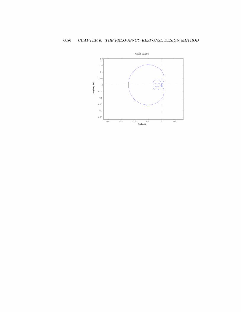
6086 CHAPTER 6. THE FREQUENCY-RESPONSE DESIGN METHOD
0.4 0.3 0.2 0.1 0 0.1
0.25
0.2
0.15
0.1
0.05
0
0.05
0.1
0.15
0.2
Nyquist Diagram
Real Axis
Imag
inar
y A
xis

6087
Figure 6.90: Nyquist plot for Problem 24
(a) Problems and Solutions for Section 6.4
24. The Nyquist plot for some actual control systems resembles the one shownin Fig.6.90. What are the gain and phase margin(s) for the system ofFig. 6.90 given that � = 0:4; � = 1:3; and � = 40o: Describe whathappens to the stability of the system as the gain goes from zero to a verylarge value. Sketch what the corresponding root locus must look like forsuch a system. Also sketch what the corresponding Bode plots would looklike for the system.
Solution :
The phase margin is de�ned as in Figure 6.34, PM = � (! = !�),but now there are several gain margins! If the system gain is increased(multiplied) by 1
j�j or decreased (divided) by j�j, then the system will gounstable. This is a conditionally stable system. See Figure 6.40 for atypical root locus of a conditionally stable system.
gain margin = -20 log j�jdB (! = !H)gain margin = +20 log j�jdB (! = !L)
For a conditionally stable type of system as in Fig. 6.40, the Bodephase plot crosses -180� twice; however, for this problem we see from theNyquist plot that it crosses 3 times! For very low values of gain, the entire

6088 CHAPTER 6. THE FREQUENCY-RESPONSE DESIGN METHOD
Nyquist plot would be shrunk, and the -1 point would occur to the left ofthe negative real axis crossing at !o, so there would be no encirclementsand the system would be stable. As the gain increases, the -1 point occursbetween !o and !L so there is an encirclement and the system is unstable.Further increase of the gain causes the -1 point to occur between !L and!H (as shown in Fig. 6.90) so there is no encirclement and the system isstable. Even more increase in the gain would cause the -1 point to occurbetween !H and the origin where there is an encirclement and the systemis unstable. The root locus would look like Fig. 6.40 except that the verylow gain portion of the loci would start in the LHP before they loop outinto the RHP as in Fig. 6.40. The Bode plot would be vaguely like thatdrawn below:
25. The Bode plot for
G(s) =100[(s=10) + 1]
s[(s=1)� 1][(s=100) + 1]
is shown in Fig. 6.91.
(a) Why does the phase start at -270o at the low frequencies?
(b) Sketch the Nyquist plot for G(s).
(c) Is the closed-loop system shown in Fig. 6.92 stable?

6089
Figure 6.91: Bode plot for Problem 25
(d) Will the system be stable if the gain is lowered by a factor of 100?Make a rough sketch of a root locus for the system and qualitativelycon�rm your answer
Solution :
(a) From the root locus, the phase at the low frequencies (! = 0+) iscalculated as :
The phase at the point fs = j!(! = 0+)g= �180�(pole : s = 1)� 90�(pole : s = 0) + 0�(zero : s = �10) + 0�(pole : s = �100)= �270�
Or, more simply, the RHP pole at s = +1 causes a �180o shift fromthe �90o that you would expect from a normal system with all thesingularities in the LHP.

6090 CHAPTER 6. THE FREQUENCY-RESPONSE DESIGN METHOD
Figure 6.92: Control system for Problem 26
(b) The Nyquist plot for G(s) :
(c) As the Nyquist shows, there is one counter-clockwise encirclement of-1.
=) N = �1
We have one pole in RHP =) P = 1
Z = N + P = �1 + 1 = 0 =) The closed-loop system is stable.
(d) The system goes unstable if the gain is lowered by a factor of 100.
26. Suppose that in Fig. 6.92,
G(s) =25(s+ 1)
s(s+ 2)(s2 + 2s+ 16):
Use MATLAB�s margin to calculate the PM and GM for G(s) and, basedon the Bode plots, conclude which margin would provide more useful in-formation to the control designer for this system.
Solution :

6091
100
80
60
40
20
0
20M
agni
tude
(dB)
101
100
101
102
270
225
180
135
90
45
Phas
e (d
eg)
Bode DiagramGm = 3.91 dB (at 4.22 rad/sec) , Pm = 101 deg (at 1.08 rad/sec)
Frequency (rad/sec)
100
80
60
40
20
0
20M
agni
tude
(dB)
101
100
101
102
270
225
180
135
90
45
Phas
e (d
eg)
From the Bode plot,
PM = 101 deg; GM = 3:9db = 1:57
Since both PM and GM are positive, we can say that the closed-loop ofthis system is stable. But GM is so small that we must be careful not toincrease the gain much, which leads the closed-loop system to be unstable.Clearly, the GM is the more important margin for this example.
27. Consider the system given in Fig. 6.93.
(a) Use MATLAB to obtain Bode plots for K = 1 and use the plots toestimate the range of K for which the system will be stable.
(b) Verify the stable range of K by using margin to determine PM forselected values of K.
(c) Use rlocus and rloc�nd to determine the values of K at the stabilityboundaries.

6092 CHAPTER 6. THE FREQUENCY-RESPONSE DESIGN METHOD
Figure 6.93: Control system for Problem 27
(d) Sketch the Nyquist plot of the system, and use it to verify the numberof unstable roots for the unstable ranges of K.
(e) Using Routh�s criterion, determine the ranges of K for closed-loopstability of this system.
Solution :
(a) The Bode plot for K = 1 is :
101 100 101102
101
100
Frequency (rad/sec)
Mag
nitu
de
Bode plot for Prob. 6.27 (a): K =1
101 100 101102
101
100
Frequency (rad/sec)
Mag
nitu
de
Bode plot for Prob. 6.27 (a): K =1
101 100 101200
190
180
170
160
ω (rad/sec)
Pha
se (d
eg)
101 100 101102
101
100
Frequency (rad/sec)
Mag
nitu
de
Bode plot for Prob. 6.27 (a): K =1
101 100 101102
101
100
Frequency (rad/sec)
Mag
nitu
de
Bode plot for Prob. 6.27 (a): K =1
101 100 101200
190
180
170
160
ω (rad/sec)
Pha
se (d
eg)

6093
From the Bode plot, the closed-loop system is unstable for K =1. But we can make the closed-system stable with positive GM byincreasing the gain K up to the crossover frequency reaches at ! =1:414 rad/sec (K = 2), where the phase plot crosses the �180� line.Therefore :
1 < K < 2 =) The closed-loop system is stable.
(b) For example, PM = 6:66 deg for K = 1:5.
80
60
40
20
0
20
Mag
nitu
de (d
B)
101
100
101
102
200
190
180
170
160
Phas
e (d
eg)
Bode DiagramGm = 2.5 dB (at 1.41 rad/sec) , Pm = 6.66 deg (at 1.08 rad/sec)
Frequency (rad/sec)
80
60
40
20
0
20
Mag
nitu
de (d
B)
101
100
101
102
200
190
180
170
160
Phas
e (d
eg)
(c) Root locus is :

6094 CHAPTER 6. THE FREQUENCY-RESPONSE DESIGN METHOD
j!-crossing :
1 +Kj! + 2
(j!)3 + (j!)2 � 2 = 0
!2 � 2K + 2 = 0
!(!2 �K) = 0
K = 2; ! = �p2; or K = 1; ! = 0
Therefore,
1 < K < 2 =) The closed-loop system is stable.

6095
(d)
i. 0 < K < 1N = 0; P = 1 =) Z = 1One unstable closed-loop root.
ii. 1 < K < 2N = �1; P = 1 =) Z = 0Stable.
iii. 2 < KN = 1; P = 1 =) Z = 2Two unstable closed-loop roots.
(e) The closed-loop transfer function of this system is :
y(s)
r(s)=
k1
s� 11 + k
1
s� 1 �s+ 2
(s+ 1)2 + 1
=K(s2 + 2s+ 2)
s3 + s2 +Ks+ 2K � 2
So the characteristic equation is :
=) s3 + s2 +Ks+ 2K � 2 = 0
Using the Routh�s criterion,
s3 : 1 Ks2 : 1 2K � 2s1 : 2�K 0s0 : 2k = 2
For stability,

6096 CHAPTER 6. THE FREQUENCY-RESPONSE DESIGN METHOD
2�K > 0
2K � 2 > 0
=) 2 > K > 1
0 < K < 1 Unstable1 < K < 2 Stable2 < K Unstable
28. Suppose that in Fig. 6.92,
G(s) =3:2(s+ 1)
s(s+ 2)(s2 + 0:2s+ 16):
Use MATLAB�smargin to calculate the PM and GM forG(s) and commenton whether you think this system will have well damped closed-loop roots.
Solution :
MATLAB�s margin plot for the given system is :
150
100
50
0
50
Mag
nitu
de (d
B)
101
100
101
102
270
225
180
135
90
45
Phas
e (d
eg)
Bode DiagramGm = 1 dB (at 4.02 rad/sec) , Pm = 92.8 deg (at 0.1 rad/sec)
Frequency (rad/sec)
150
100
50
0
50
Mag
nitu
de (d
B)
101
100
101
102
270
225
180
135
90
45
Phas
e (d
eg)

6097
From the MATLAB margin routine, PM = 92:8o . Based on this result,Fig. 6.36 suggests that the damping will be = 1; that is, the roots will bereal. However, closer inspection shows that a very small increase in gainwould result in an instability from the resonance leading one to believethat the damping of these roots is very small. Use of MATLAB�s damproutine on the closed loop system con�rms this where we see that there aretwo real poles (� = 1) and two very lightly damped poles with � = 0:0027:This is a good example where one needs to be careful to not use Matlabwithout thinking.
29. For a given system, show that the ultimate period Pu and the correspond-ing ultimate gain Ku for the Zeigler-Nichols method can be found usingthe following:
(a) Nyquist diagram
(b) Bode plot
(c) root locus.
Solution :
(a) See sketch below.
Pu =2�
!u
(b) See sketch below.

6098 CHAPTER 6. THE FREQUENCY-RESPONSE DESIGN METHOD
Pu =2�
!u
(c)
1 +KuG(j!u) = 0
1 +KuRe[G(j!u)] +Kuj Im[G(j!u)] = 0
Ku = �1
Re[G(j!u)]
Im[G(j!u)] = 0; or Pu =2�
!u

6099
30. If a system has the open-loop transfer function
G(s) =!2n
s(s+ 2�!n)
with unity feedback, then the closed-loop transfer function is given by
T (s) =!2n
s2 + 2�!ns+ !2n:
Verify the values of the PM shown in Fig. 6.36 for � = 0:1, 0.4, and 0.7.
Solution :
G(s) =!2n
s(s+ 2�!n); T (s) =
G(s)
1 +G(s)=
!2ns2 + 2�!ns+ !2n
� PM from Eq. 6.32 PM from Fig. 6.36 PM from Bode plot0.1 10� 10� 11.4� (! = 0:99 rad/sec)0.4 40� 44� 43.1� (! = 0:85 rad/sec)0.7 70� 65� 65.2� (! = 0:65 rad/sec)
31. Consider the unity feedback system with the open-loop transfer function
G(s) =K
s(s+ 1)[(s2=25) + 0:4(s=5) + 1]:
(a) Use MATLAB to draw the Bode plots for G(j!) assuming K = 1.

6100 CHAPTER 6. THE FREQUENCY-RESPONSE DESIGN METHOD
(b) What gain K is required for a PM of 45�? What is the GM for thisvalue of K?
(c) What is Kv when the gain K is set for PM = 45�?
(d) Create a root locus with respect to K, and indicate the roots for aPM of 45�.
Solution :
(a) The Bode plot for K = 1 is shown below and we can see from marginthat it results in a PM = 48o.
102 101 100 101 1021010
105
100
105
ω (rad/sec)
Mag
nitu
de
Bode plot for Prob. 6.31
102 101 100 101 1021010
105
100
105
ω (rad/sec)
Mag
nitu
de
Bode plot for Prob. 6.31
102 101 100 101 102400
300
200
100
0
ω (rad/sec)
Pha
se (d
eg)
102 101 100 101 1021010
105
100
105
ω (rad/sec)
Mag
nitu
de
Bode plot for Prob. 6.31
102 101 100 101 1021010
105
100
105
ω (rad/sec)
Mag
nitu
de
Bode plot for Prob. 6.31
102 101 100 101 102400
300
200
100
0
ω (rad/sec)
Pha
se (d
eg)
(b) Although di¢ cult to read the plot above, it is clear that a very slightincrease in gain will lower the PM to 45o, so try K = 1:1: The marginroutine shows that this yields PM = 45o and GM = 15 db.
(c) Kv = lims!0fsKG(s)g = K = 1:1 when K is set for PM=45�
Kv = 1:1

6101
(d) The characteristic equation for PM of 45� :
1 +1:1
s(s+ 1)h�
s5
�2+ 0:4
�s5
�+ 1i = 0
=) s4 + 3s3 + 27s2 + 25s+ 27:88 = 0
=) s = �1:03� j4:78; �0:47� j0:97
32. For the system depicted in Fig. 6.94(a), the transfer-function blocks arede�ned by
G(s) =1
(s+ 2)2(s+ 4)and H(s) =
1
s+ 1:
(a) Using rlocus and rloc�nd, determine the value of K at the stabilityboundary.
(b) Using rlocus and rloc�nd, determine the value of K that will produceroots with damping corresponding to � = 0:707.
(c) What is the gain margin of the system if the gain is set to the valuedetermined in part (b)? Answer this question without using anyfrequency response methods.
(d) Create the Bode plots for the system, and determine the gain marginthat results for PM = 65�. What damping ratio would you expectfor this PM?

6102 CHAPTER 6. THE FREQUENCY-RESPONSE DESIGN METHOD
Figure 6.94: Block diagram for Problem 32: (a) unity feedback; (b) H(s) infeedback
(e) Sketch a root locus for the system shown in Fig. 6.94(b).. How doesit di¤er from the one in part (a)?
(f) For the systems in Figs. 6.94(a) and (b), how does the transfer func-tion Y2(s)=R(s) di¤er from Y1(s)=R(s)? Would you expect the stepresponse to r(t) be di¤erent for the two cases?
Solution :
(a) The root locus crosses j! axis at s0 = j2.
K =1
jH(s0)G(s0)jjs0=j2
= jj2 + 1j jj2 + 4j jj2 + 2j2
=) K = 80

6103
(b)� = 0:707 =) 0:707 = sin � =) � = 45�
From the root locus given,
s1 = �0:91 + j0:91
K =1
jH(s1)G(s1)jjs1=�0:91+j0:91
= j0:01 + j0:91j j3:09 + j0:91j j1:09 + j0:91j2
=) K = 5:9
(c)
GM =Ka
Kb=80
5:9= 13:5
(d) From the Root Locus :
G(s)H(s) =1
(s+ 1)(s+ 2)2(s+ 4)
PM=65� when K = 30. Instability occurs when K = 80:0.
=) GM = 2:67
We approximate the damping ratio by � ' PM100
� ' 65
100= 0:65

6104 CHAPTER 6. THE FREQUENCY-RESPONSE DESIGN METHOD
102 101 100 101 1021010
105
100
Frequency (rad/sec)
Mag
nitu
de
Bode plot for Prob. 6.32
102 101 100 101 1021010
105
100
Frequency (rad/sec)
Mag
nitu
de
Bode plot for Prob. 6.32
102 101 100 101 102400
300
200
100
0
ω (rad/sec)
Pha
se (d
eg)
102 101 100 101 1021010
105
100
Frequency (rad/sec)
Mag
nitu
de
Bode plot for Prob. 6.32
102 101 100 101 1021010
105
100
Frequency (rad/sec)
Mag
nitu
de
Bode plot for Prob. 6.32
102 101 100 101 102400
300
200
100
0
ω (rad/sec)
Pha
se (d
eg)
(e) The root locus for Fig.6.94(a) is the same as that of Fig.6.94(b).
(f)
Y1(s)
R(s)=
KG(s)H(s)
1 +KG(s)H(s)=
K
(s+ 1)(s+ 2)2(s+ 4) +K
Y2(s)
R(s)=
KG(s)
1 +KG(s)H(s)=
K(s+ 1)
(s+ 1)(s+ 2)2(s+ 4) +K
Y1(s)R(s) and
Y2(s)R(s) have the same closed-loop poles. However,
Y2(s)R(s) has
a zero, while Y1(s)R(s) doesn�t have a zero. We would therefore expect
more overshoot from system (b).
33. For the system shown in Fig. 6.95, use Bode and root-locus plots to deter-mine the gain and frequency at which instability occurs. What gain (orgains) gives a PM of 20�? What is the gain margin when PM = 20�?
Solution :

6105
Figure 6.95: Control system for Problem 33
102 101 100 101 1021010
105
100
105
ω (rad/sec)
Mag
nitu
de
Bode plot for Prob. 6.33
102 101 100 101 1021010
105
100
105
ω (rad/sec)
Mag
nitu
de
Bode plot for Prob. 6.33
102 101 100 101 102300
250
200
150
100
ω (rad/sec)
Pha
se (d
eg)
102 101 100 101 1021010
105
100
105
ω (rad/sec)
Mag
nitu
de
Bode plot for Prob. 6.33
102 101 100 101 1021010
105
100
105
ω (rad/sec)
Mag
nitu
de
Bode plot for Prob. 6.33
102 101 100 101 102300
250
200
150
100
ω (rad/sec)
Pha
se (d
eg)

6106 CHAPTER 6. THE FREQUENCY-RESPONSE DESIGN METHOD
The system with K = 1 gives,
GM = 52 (! = 5 rad/sec)
PM = 10� (! = 0:165 rad/sec)
Therefore, instability occurs at K0 = 52 and ! = 5 rad/sec.
From the Bode plot, a PM of 20� is given by,
K1 = 3:9 (! = 0:33 rad/sec); GM =52
3:9= 13
K2 = 49 (! = 4:6 rad/sec); GM =52
49= 1:06
34. A magnetic tape-drive speed-control system is shown in Fig. 6.96. Thespeed sensor is slow enough that its dynamics must be included. Thespeed-measurement time constant is �m = 0:5 sec; the reel time constantis � r = J=b = 4 sec, where b = the output shaft damping constant =1 N �m � sec; and the motor time constant is �1 = 1 sec.
(a) Determine the gain K required to keep the steady-state speed errorto less than 7% of the reference-speed setting.
(b) Determine the gain and phase margins of the system. Is this a goodsystem design?
Solution :
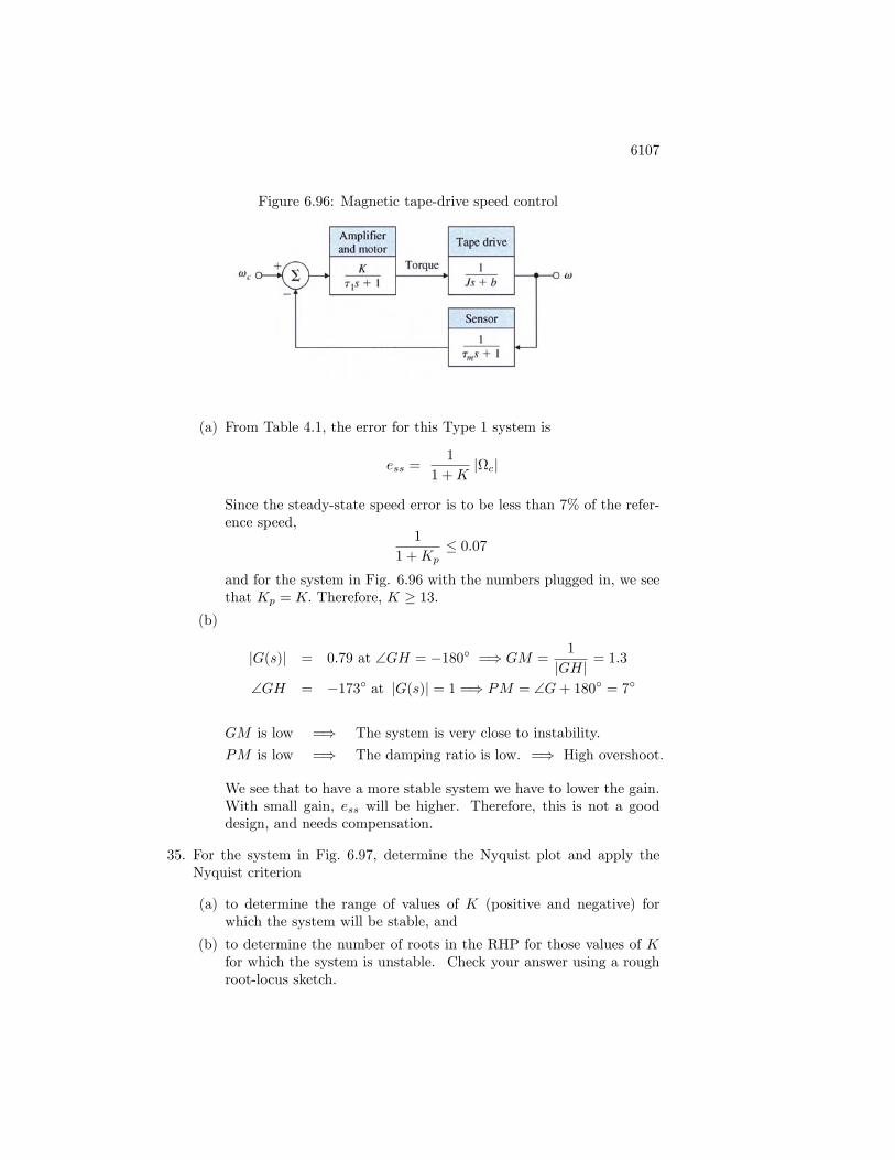
6107
Figure 6.96: Magnetic tape-drive speed control
(a) From Table 4.1, the error for this Type 1 system is
ess =1
1 +Kjcj
Since the steady-state speed error is to be less than 7% of the refer-ence speed,
1
1 +Kp� 0:07
and for the system in Fig. 6.96 with the numbers plugged in, we seethat Kp = K: Therefore, K � 13:
(b)
jG(s)j = 0:79 at \GH = �180� =) GM =1
jGHj = 1:3
\GH = �173� at jG(s)j = 1 =) PM = \G+ 180� = 7�
GM is low =) The system is very close to instability.
PM is low =) The damping ratio is low. =) High overshoot.
We see that to have a more stable system we have to lower the gain.With small gain, ess will be higher. Therefore, this is not a gooddesign, and needs compensation.
35. For the system in Fig. 6.97, determine the Nyquist plot and apply theNyquist criterion
(a) to determine the range of values of K (positive and negative) forwhich the system will be stable, and
(b) to determine the number of roots in the RHP for those values of Kfor which the system is unstable. Check your answer using a roughroot-locus sketch.

6108 CHAPTER 6. THE FREQUENCY-RESPONSE DESIGN METHOD
Figure 6.97: Control system for Problems 35, 69, and 70
Solution :
(a) & b.
KG(s) = K3
s(s+ 1)(s+ 3)
From the Nyquist plot above, we see that:
i.
�1 < � 1K< �1
4=) 0 < K < 4
There are no RHP open loop roots, hence P = 0 for all cases.For 0 < K < 4; no encirclements of -1 so N = 0,
N = 0; P = 0 =) Z = 0
The closed-loop system is stable. No roots in RHP.
ii.
�14< � 1
K< 0 =) 4 < K <1

6109
Two encirclements of the -1 point, hence
N = 2; P = 0 =) Z = 2
Two closed-loop roots in RHP.
iii.
0 < � 1K
=) K < 0
N = 1; P = 0 =) Z = 1
One closed-loop root in RHP.
The root loci below show the same results.
36. For the system shown in Fig. 6.98, determine the Nyquist plot and applythe Nyquist criterion.
(a) to determine the range of values of K (positive and negative) forwhich the system will be stable, and
(b) to determine the number of roots in the RHP for those values of Kfor which the system is unstable. Check your answer using a roughroot-locus sketch.
Solution :
(a) & b.
KG(s) = Ks+ 1
(s� 1)2

6110 CHAPTER 6. THE FREQUENCY-RESPONSE DESIGN METHOD
Figure 6.98: Control system for Problem 36
From the Nyquist plot we see that:
i.
�1 < � 1K< �1
2=) 0 < K < 2
N = 0; P = 2 =) Z = 2
Two closed-loop roots in RHP.
ii.
�12< � 1
K< 0 =) 2 < K
N = �2; P = 2 =) Z = 0
The closed-loop system is stable.
iii.
0 < � 1K< 1 =) K < �1
N = �1; P = 2 =) Z = 1
One closed-loop root in RHP.

6111
Figure 6.99: Control system for Problem 37
iv.
1 < � 1K<1 =) �1 < K < 0
N = 0; P = 2 =) Z = 2
Two closed-loop roots in RHP.
These results are con�rmed by looking at the root loci below:
37. For the system shown in Fig. 6.99, determine the Nyquist plot and applythe Nyquist criterion.
(a) to determine the range of values of K (positive and negative) forwhich the system will be stable, and
(b) to determine the number of roots in the RHP for those values of Kfor which the system is unstable. Check your answer using a roughroot-locus sketch.
Solution :

6112 CHAPTER 6. THE FREQUENCY-RESPONSE DESIGN METHOD
(a) & b.
KG(s) = Ks� 1(s+ 1)2
From the Nyquist plot we see that:
i.�1 < � 1
K< �1 =) 0 < K < 1
N = 0; P = 0 =) Z = 0
The closed-loop system is stable.
ii.�1 < � 1
K< 0 =) 1 < K
N = 1; P = 0 =) Z = 1
One closed-loop root in RHP.
iii.0 < � 1
K<1
2=) K < �2
N = 2; P = 0 =) Z = 2
Two closed-loop roots in RHP.
iv.1
2< � 1
K=) �2 < K < 0
N = 0; P = 0 =) Z = 0
The closed-loop system is stable.
These results are con�rmed by looking at the root loci below:

6113
38. The Nyquist diagrams for two stable, open-loop systems are sketched inFig. 6.100. The proposed operating gain is indicated as K0, and arrowsindicate increasing frequency. In each case give a rough estimate of thefollowing quantities for the closed-loop (unity feedback) system:
(a) phase margin
(b) damping ratio
(c) range of gain for stability (if any)
(d) system type (0, 1, or 2).
Solution :

6114 CHAPTER 6. THE FREQUENCY-RESPONSE DESIGN METHOD
Figure 6.100: Nyquist plots for Problem 38
For both, with K = K0:
N = 0; P = 0 =) Z = 0
Therefore, the closed-loop system is stable.
Fig.6.102(a) Fig.6.102(b)a. PM '17� '45�b. Damping ratio 0.17(' 17
100 ) 0.45(' 45100 )
c. To determine the range of gain for stability, call the value of K wherethe plots cross the negative real axis as K1: For case (a), K > K1 forstability because gains lower than this amount will cause the -1 point tobe encircled. For case (b), K < K1 for stability because gains greaterthan this amount will cause the -1 point to be encircled.
d. For case (a), the 360o loop indicates two poles at the origin, hence thesystem is Type 2. For case (b), the 180o loop indicates one pole at theorigin, hence the system is Type 1.
39. The steering dynamics of a ship are represented by the transfer function
V (s)
�r(s)= G(s) =
K[�(s=0:142) + 1]s(s=0:325 + 1)(s=0:0362) + 1)
;
where v is the ship�s lateral velocity in meters per second, and �r is therudder angle in radians.
(a) Use the MATLAB command bode to plot the log magnitude andphase of G(j!) for K = 0:2
(b) On your plot, indicate the crossover frequency, PM, and GM,
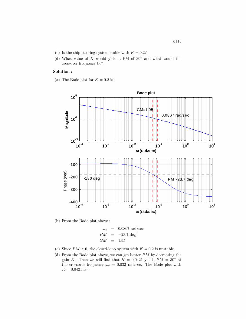
6115
(c) Is the ship steering system stable with K = 0:2?
(d) What value of K would yield a PM of 30o and what would thecrossover frequency be?
Solution :
(a) The Bode plot for K = 0:2 is :
104 103 102 101 100 101105
100
105
ω (rad/sec)
Mag
nitu
de
Bode plot
104 103 102 101 100 101105
100
105
ω (rad/sec)
Mag
nitu
de
Bode plot
104 103 102 101 100 101400
300
200
100
ω (rad/sec)
Pha
se (d
eg)
104 103 102 101 100 101105
100
105
ω (rad/sec)
Mag
nitu
de
Bode plot
104 103 102 101 100 101105
100
105
ω (rad/sec)
Mag
nitu
de
Bode plot
0.0867 rad/secGM=1.95
104 103 102 101 100 101400
300
200
100
ω (rad/sec)
Pha
se (d
eg)
180 deg PM=23.7 deg
(b) From the Bode plot above :
!c = 0:0867 rad/sec
PM = �23:7 degGM = 1:95
(c) Since PM < 0, the closed-loop system with K = 0:2 is unstable.
(d) From the Bode plot above, we can get better PM by decreasing thegain K. Then we will �nd that K = 0:0421 yields PM = 30� atthe crossover frequency !c = 0:032 rad/sec. The Bode plot withK = 0:0421 is :

6116 CHAPTER 6. THE FREQUENCY-RESPONSE DESIGN METHOD
100
50
0
50
Mag
nitu
de (d
B)
103
102
101
100
101
0
90
180
270
Phas
e (d
eg)
Bode DiagramGm = 7.68 dB (at 0.0576 rad/sec) , Pm = 30 deg (at 0.0321 rad/sec)
Frequency (rad/sec)
100
50
0
50
Mag
nitu
de (d
B)
103
102
101
100
101
0
90
180
270
Phas
e (d
eg)
40. For the open-loop system
KG(s) =K(s+ 1)
s2(s+ 10)2:
Determine the value for K at the stability boundary and the values of Kat the points where PM = 30�.
Solution :
The bode plot of this system with K = 1 is :

6117
150
100
50
0
50
100M
agni
tude
(dB)
102
101
100
101
102
270
225
180
135
Phas
e (d
eg)
Bode DiagramGm = 64.1 dB (at 8.94 rad/sec) , Pm = 4.58 deg (at 0.1 rad/sec)
Frequency (rad/sec)
150
100
50
0
50
100M
agni
tude
(dB)
102
101
100
101
102
270
225
180
135
Phas
e (d
eg)
Since GM = 64:1 db (' 1600), the range of K for stability is :
K < 1600
From the Bode plot, the magnitude at the frequency with �150� phaseis 0:0188 (�34:5 dB) at 0:8282 rad/sec and 0:00198 (�54:1 db) at 4:44rad/sec. Therefore, the values of K at the points where PM = 30� is :
K =1
0:0188= 53:2;
K =1
0:00198= 505
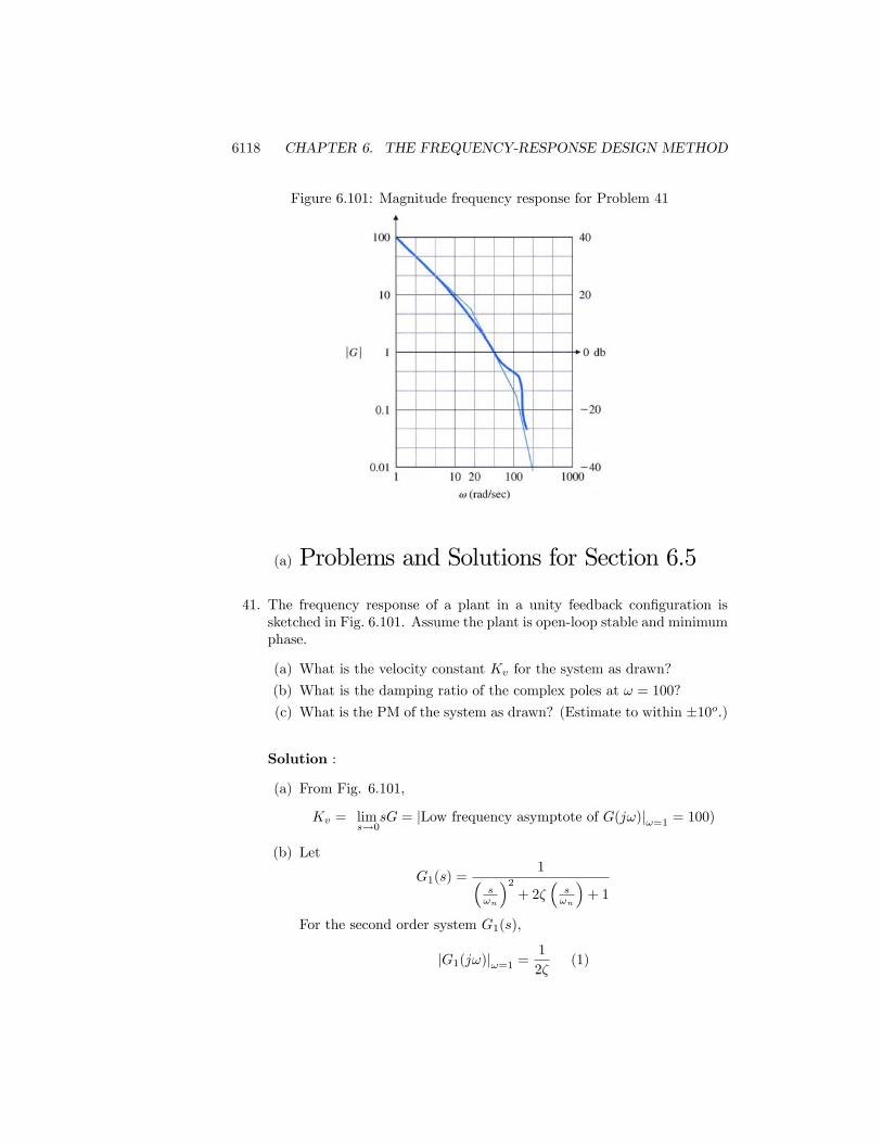
6118 CHAPTER 6. THE FREQUENCY-RESPONSE DESIGN METHOD
Figure 6.101: Magnitude frequency response for Problem 41
(a) Problems and Solutions for Section 6.5
41. The frequency response of a plant in a unity feedback con�guration issketched in Fig. 6.101. Assume the plant is open-loop stable and minimumphase.
(a) What is the velocity constant Kv for the system as drawn?
(b) What is the damping ratio of the complex poles at ! = 100?
(c) What is the PM of the system as drawn? (Estimate to within �10o.)
Solution :
(a) From Fig. 6.101,
Kv = lims!0
sG = jLow frequency asymptote of G(j!)j!=1 = 100)
(b) Let
G1(s) =1�
s!n
�2+ 2�
�s!n
�+ 1
For the second order system G1(s),
jG1(j!)j!=1 =1
2�(1)

6119
From Fig. 6.101 :
jG1(j!)j!=100 =jG(j!)j!=100
jAsymptote of G(j!)j!=100�=0:4
0:2= 2 (2)
From (1) and (2) we have :
1
2�= 2 =) � = 0:25
(c) Since the plant is a minimum phase system, we can apply the Bode�sapproximate gain-phase relationship.
When jGj = 1, the slope of jGj curve is �= -2.
=) \G(j!) �= �2� 90� = �180�
PM �= \G(j!) + 180� = 0�
Note : Actual PM by Matlab calculation is 6.4�; so this approxima-tion is within the desired accuracy.
42. For the system
G(s) =100(s=a+ 1)
s(s+ 1)(s=b+ 1);
where b = 10a, �nd the approximate value of a that will yield the best PMby sketching only candidate values of the frequency response magnitude.
Solution :

6120 CHAPTER 6. THE FREQUENCY-RESPONSE DESIGN METHOD
101 100 101 102 103
100
Frequency (rad/sec)
Mag
nitu
de
Bode Diagrams
101 100 101 102 103200
180
160
140
120
100
80
ω (rad/sec)
Pha
se (d
eg)
101 100 101 102 103
100
Frequency (rad/sec)
Mag
nitu
de
Bode Diagrams
101 100 101 102 103
100
Frequency (rad/sec)
Mag
nitu
de
Bode Diagrams
101 100 101 102 103200
180
160
140
120
100
80
ω (rad/sec)
Pha
se (d
eg) a=3.16
a=10
Uncompensated
101 100 101 102 103
100
Frequency (rad/sec)
Mag
nitu
de
Bode Diagrams
a=3.16
a=10Uncompensated
Without the zero and pole that contain the a & b terms, the plotof jGj shows a slope of �2 at the jGj = 1 crossover at 10 rad/sec. Weclearly need to install the zero and pole with the a & b terms somewhereat frequencies greater 1 rad/sec. This will increase the slope from -2 to-1 between the zero and pole. So the problem simpli�es to selecting a sothat the -1 slope region between the zero and pole brackets the crossoverfrequency. That scenario will maximize the PM. Referring to the plotsabove, we see that 3:16 < a < 10, makes the slope of the asymptote of jGjbe �1 at the crossover and represent the two extremes of possibilities for a-1 slope. The maximum PM will occur half way between these extremeson a log scale, or
=) a =p3:16� 10 = 5:6

6121
Note : Actual PM is as follows :
PM = 46:8� for a = 3:16 (!c = 25:0 rad/sec)
PM = 58:1� for a = 5:6 (!c = 17:8 rad/sec)
PM = 49:0� for a = 10 (!c = 12:6 rad/sec)

6122 CHAPTER 6. THE FREQUENCY-RESPONSE DESIGN METHOD
Problem and Solution for Section 6.6
43. For the open-loop system
KG(s) =K(s+ 1)
s2(s+ 10)2:
Determine the value for K that will yield PM � 30� and the maximumpossible closed-loop bandwidth. Use MATLAB to �nd the bandwidth.
Solution :
From the result of Problem 6.39., the value of K that will yield PM � 30�is :
53:2 � K � 505
The maximum closed-loop bandwidth will occur with the maximum gainK within the allowable region; therefore, the maximum bandwidth willoccur with K = 505: The Bode plot of the closed loop system with K =505 is :
100
50
0
50
100
150
Mag
nitu
de (d
B)
102
101
100
101
102
270
225
180
135
Phas
e (d
eg)
Bode DiagramGm = 10 dB (at 8.94 rad/sec) , Pm = 30 deg (at 4.36 rad/sec)
Frequency (rad/sec)
100
50
0
50
100
150
Mag
nitu
de (d
B)
102
101
100
101
102
270
225
180
135
Phas
e (d
eg)

6123
Looking at the point with Magnitude 0.707(-3 db), the maximum possibleclosed-loop bandwidth is :
!BW; max ' 7:7 rad/sec.
Problems and Solutions for Section 6.744. For the lead compensator
D(s) =Ts+ 1
�Ts+ 1;
where � < 1.
(a) Show that the phase of the lead compensator is given by
� = tan�1(T!)� tan�1(�T!):
(b) Show that the frequency where the phase is maximum is given by
!max =1
Tp�;
and that the maximum phase corresponds to
sin�max =1� �1 + �
:
(c) Rewrite your expression for !max to show that the maximum-phasefrequency occurs at the geometric mean of the two corner frequencieson a logarithmic scale:
log!max =1
2
�log
1
T+ log
1
�T
�:
(d) To derive the same results in terms of the pole-zero locations, rewriteD(s) as
D(s) =s+ z
s+ p;
and then show that the phase is given by
� = tan�1�!
jzj
�� tan�1
�!
jpj
�;
such that!max =
pjzjjpj:
Hence the frequency at which the phase is maximum is the squareroot of the product of the pole and zero locations.

6124 CHAPTER 6. THE FREQUENCY-RESPONSE DESIGN METHOD
Solution :
(a) The frequency response is obtained by letting s = j!,
D(j!) = KTj! + 1
�Tj! + 1
The phase is given by,� = tan�1(T!)� tan�1(�T!)(b) Using the trigonometric relationship,
tan(A�B) = tan(A)� tan(B)1 + tan(A) tan(B)
then
tan(�) =T! � �T!1� �T 2!2
and since,
sin2(�) =tan2(�)
1 + tan2(�)
then
sin(�) =
s!2T 2(1� �)2
1 + �2!4T 4 + (1 + �2)!2T 2
To determine the frequency at which the phase is a maximum, let usset the derivative with respect to ! equal to zero,
d sin(�)
d!= 0
which leads to2!T 2(1� �)2(1� �!4T 4) = 0
The value ! = 0 gives the maximum of the function and setting thesecond part of the above equation to zero then,
!4 =1
�2T 4
or!max =
1p�T
The maximum phase contribution, that is, the peak of the \D(s)curve corresponds to,
sin�max =1� �1 + �
or
� =1� sin�max1 + sin�max
tan�max =!maxT � �!maxT1 + !2maxT
2=1� �2p�

6125
(c) The maximum frequency occurs midway between the two break fre-quencies on a logarithmic scale,
log!max = log
1pTp�T
= log1pT+ log
1p�T
=1
2
�log
1
T+ log
1
�T
�as shown in Fig. 6.53.
(d) Alternatively, we may state these results in terms of the pole-zerolocations. Rewrite D(s) as,
D(s) = K(s+ z)
(s+ p)
then
D(j!) = K(j! + z)
(j! + p)
and
� = tan�1�!
jzj
�� tan�1
�!
jpj
�or
tan� =
!jzj �
!jpj
1 + !jzj
!jpj
Setting the derivative of the above equation to zero we �nd,�!
jzj �!
jpj
��1 +
!2
jzj jpj
�� 2!
jzj jpj
�!
jzj �!
jpj
�= 0
and!max =
pjzj jpj
and
log!max =1
2(log jzj+ log jpj)
Hence the frequency at which the phase is maximum is the squareroot of the product of the pole and zero locations.
45. For the third-order servo system
G(s) =50; 000
s(s+ 10)(s+ 50):

6126 CHAPTER 6. THE FREQUENCY-RESPONSE DESIGN METHOD
Design a lead compensator so that PM �50� and !BW � 20 rad/sec usingBode plot sketches, then verify and re�ne your design using Matlab.
Solution :
Let�s design the lead compensator so that the system has PM � 50� &!WB ' !c � 20 rad/sec.The Bode plot of the given system is :
100
50
0
50
100
Mag
nitu
de (d
B)
101
100
101
102
103
270
225
180
135
90
Phas
e (d
eg)
Bode Diagram
Frequency (rad/sec)
100
50
0
50
100
Mag
nitu
de (d
B)
101
100
101
102
103
270
225
180
135
90
Phas
e (d
eg)
Start with a lead compensator design with :
D(s) =Ts+ 1
�Ts+ 1(� < 1)
Since the open-loop crossover frequency !c(' !BW ) is already above 20rad/sec, we are going to just add extra phase around ! = !c in order tosatisfy PM = 50�.
Let�s add phase lead � 60�. From Fig. 6.54,
1
�' 20 =) choose � = 0:05

6127
To apply maximum phase lead at ! = 20 rad/sec;
! =1p�T
= 20 =) 1
T= 4:48;
1
�T= 89:4
Therefore by applying the lead compensator with some gain adjustments:
D(s) = 0:12�s
4:5+ 1
s
90+ 1
we get the compensated system with :
PM = 65�; !c = 22 rad/sec, so that !BW & 25 rad/sec.
The Bode plot with designed compensator is :
100
50
0
50
Mag
nitu
de (d
B)
101
100
101
102
103
270
225
180
135
90
45
Phas
e (d
eg)
Bode DiagramGm = 15.9 dB (at 72.6 rad/sec) , Pm = 65.3 deg (at 22 rad/sec)
Frequency (rad/sec)
100
50
0
50
Mag
nitu
de (d
B)
101
100
101
102
103
270
225
180
135
90
45
Phas
e (d
eg)

6128 CHAPTER 6. THE FREQUENCY-RESPONSE DESIGN METHOD
Figure 6.102: Control system for Problem 46
46. For the system shown in Fig. 6.102, suppose that
G(s) =5
s(s+ 1)(s=5 + 1):
Design a lead compensation D(s) with unity DC gain so that PM � 40�using Bode plot sketches, then verify and re�ne your design using Matlab.What is the approximate bandwidth of the system?
Solution :
Start with a lead compensator design with :
D(s) =Ts+ 1
�Ts+ 1
which has unity DC gain with � < 1.
The Bode plot of the given system is :

6129
100
50
0
50
100M
agni
tude
(dB)
102
101
100
101
102
270
225
180
135
90
Phas
e (d
eg)
Bode DiagramGm = 1.58 dB (at 2.24 rad/sec) , Pm = 3.94 deg (at 2.04 rad/sec)
Frequency (rad/sec)
100
50
0
50
100M
agni
tude
(dB)
102
101
100
101
102
270
225
180
135
90
Phas
e (d
eg)
Since PM = 3:9�, let�s add phase lead � 60�. From Fig. 6.53,
1
�' 20 =) choose � = 0:05
To apply maximum phase lead at ! = 10 rad/sec;
! =1p�T
= 10 =) 1
T= 2:2;
1
�T= 45
Therefore by applying the lead compensator :
D(s) =
s
2:2+ 1
s
45+ 1
we get the compensated system with :
PM = 40�; !c = 2:5
The Bode plot with designed compensator is :

6130 CHAPTER 6. THE FREQUENCY-RESPONSE DESIGN METHOD
150
100
50
0
50
100
Mag
nitu
de (d
B)
102
101
100
101
102
103
270
225
180
135
90
Phas
e (d
eg)
Bode DiagramGm = 24.1 dB (at 12.8 rad/sec) , Pm = 40.2 deg (at 2.49 rad/sec)
Frequency (rad/sec)
150
100
50
0
50
100
Mag
nitu
de (d
B)
102
101
100
101
102
103
270
225
180
135
90
Phas
e (d
eg)
From Fig. 6.51, we see that !BW ' 2� !c ' 5 rad/sec.
47. Derive the transfer function from Td to � for the system in Fig. 6.70. Thenapply the Final Value Theorem (assuming Td = constant) to determinewhether �(1) is nonzero for the following two cases:
(a) When D(s) has no integral term: lims!0D(s) = constant;
(b) When D(s) has an integral term:
D(s) =D0(s)
s;
where lims!0D0(s) = constant.
Solution :
The transfer function from Td to � :
�(s)
Td(s)=
0:9s2
1 + 0:9s2
2s+2D(s)

6131
where Td(s) = jTdj =s.
(a) Using the �nal value theorem :
�(1) = limt!1
�(t) = lims!0
s�(t) = lims!0
0:9s2
s2(s+2)+1:8D(s)s2(s+2)
jTdjs
=jTdj
lims!0
D(s)=
jTdjconstant
6= 0
Therefore, there will be a steady state error in � for a constant Tdinput if there is no integral term in D(s).
(b)
�(1) = limt!1
�(t) = lims!0
s�(t) = lims!0
0:9s2
s3(s+2)+1:8D0(s)s3(s+2)
jTdjs
=0
1:8lims!0
D0(s)= 0
So when D(s) contains an integral term, a constant Td input willresult in a zero steady state error in �.
48. The inverted pendulum has a transfer function given by Eq. (2.31), whichis similar to
G(s) =1
s2 � 1 :
(a) Design a lead compensator to achieve a PM of 30� using Bode plotsketches, then verify and re�ne your design using MATLAB.
(b) Sketch a root locus and correlate it with the Bode plot of the system.
(c) Could you obtain the frequency response of this system experimen-tally?
Solution :
(a) Design the lead compensator :
D(s) = KTs+ 1
�Ts+ 1
such that the compensated system has PM ' 30� & !c ' 1 rad/sec.(Actually, the bandwidth or speed of response was not speci�ed, soany crossover frequency would satisfy the problem statement.)
� =1� sin(30�)1 + sin(30�)
= 0:32

6132 CHAPTER 6. THE FREQUENCY-RESPONSE DESIGN METHOD
To apply maximum phase lead at ! = 1 rad/sec;
! =1p�T
= 1 =) 1
T= 0:57;
1
�T= 1:77
Therefore by applying the lead compensator :
D(s) = K
s
0:57+ 1
s
1:77+ 1
By adjusting the gain K so that the crossover frequency is around 1rad/sec, K = 1:13 results in :
PM = 30:8�
The Bode plot of compensated system is :
80
60
40
20
0
20
Mag
nitu
de (d
B)
102
101
100
101
102
180
170
160
150
140
Phas
e (d
eg)
Bode DiagramGm = 1.06 dB (at 0 rad/sec) , Pm = 30.8 deg (at 0.986 rad/sec)
Frequency (rad/sec)
80
60
40
20
0
20
Mag
nitu
de (d
B)
102
101
100
101
102
180
170
160
150
140
Phas
e (d
eg)
(b) Root Locus of the compensated system is :

6133
and con�rms that the system yields all stable roots with reasonabledamping. However, it would be a better design if the gain was raisedsome in order to increase the speed of response of the slow real root.A small decrease in the damping of the complex roots will result.
(c) No, because the sinusoid input will cause the system to blow up be-cause the open loop system is unstable. In fact, the system will�blow up�even without the sinusoid applied. Or, a better descrip-tion would be that the pendulum will fall over until it hits the table.
49. The open-loop transfer function of a unity feedback system is
G(s) =K
s(s=5 + 1)(s=50 + 1):
(a) Design a lag compensator for G(s) using Bode plot sketches so thatthe closed-loop system satis�es the following speci�cations:
i. The steady-state error to a unit ramp reference input is less than0.01.
ii. PM � = 40�
(b) Verify and re�ne your design using Matlab.
Solution :
Let�s design the lag compensator :
D(s) =Ts+ 1
�Ts+ 1; � > 1

6134 CHAPTER 6. THE FREQUENCY-RESPONSE DESIGN METHOD
From the �rst speci�cation,
Steady-state error to unit ramp = lims!0
s
���� D(s)G(s)
1 +D(s)G(s)
1
s2� 1
s2
���� < 0:01=) 1
K< 0:01
=) Choose K = 150
Uncompensated, the crossover frequency with K = 150 is too high for agood PM . With some trial and error, we �nd that the lag compensator,
D(s) =
s
0:2+ 1
s
0:01+ 1
will lower the crossover frequency to !c ' 4:46 rad/sec where the PM =40:7�.
150
100
50
0
50
100
150
Mag
nitu
de (d
B)
104
103
102
101
100
101
102
103
270
225
180
135
90
Phas
e (d
eg)
Bode DiagramGm = 18.9 dB (at 15.5 rad/sec) , Pm = 40.7 deg (at 4.46 rad/sec)
Frequency (rad/sec)
150
100
50
0
50
100
150
Mag
nitu
de (d
B)
104
103
102
101
100
101
102
103
270
225
180
135
90
Phas
e (d
eg)

6135
50. The open-loop transfer function of a unity feedback system is
G(s) =K
s(s=5 + 1)(s=200 + 1):
(a) Design a lead compensator for G(s) using Bode plot sketches so thatthe closed-loop system satis�es the following speci�cations:
i. The steady-state error to a unit ramp reference input is less than0.01.
ii. For the dominant closed-loop poles the damping ratio � � 0:4.
(b) Verify and re�ne your design using Matlab including a direct com-putation of the damping of the dominant closed-loop poles.
Solution :
Let�s design the lead compensator :
D(s) =Ts+ 1
�Ts+ 1; � < 1
From the �rst speci�cation,
Steady-state error to unit ramp = lims!0
s
���� D(s)G(s)
1 +D(s)G(s)
1
s2� 1
s2
���� < 0:01=) 1
K< 0:01
=) Choose K = 150
From the approximation � ' PM
100, the second speci�cation implies PM �
40. After trial and error, we �nd that the compensator,
D(s) =
s
10+ 1
s
100+ 1
results in a PM = 42:5� and a crossover frequency !c ' 51:2 rad/sec asshown by the margin output:

6136 CHAPTER 6. THE FREQUENCY-RESPONSE DESIGN METHOD
150
100
50
0
50
100
Mag
nitu
de (d
B)
101
100
101
102
103
104
270
225
180
135
90
Phas
e (d
eg)
Bode DiagramGm = 13.3 dB (at 136 rad/sec) , Pm = 42.5 deg (at 52.2 rad/sec)
Frequency (rad/sec)
150
100
50
0
50
100
Mag
nitu
de (d
B)
101
100
101
102
103
104
270
225
180
135
90
Phas
e (d
eg)
and the use of damp veri�es the damping to be � = 0:42 for the complexclosed-loop roots which exceeds the requirement.
51. A DC motor with negligible armature inductance is to be used in a positioncontrol system. Its open-loop transfer function is given by
G(s) =50
s(s=5 + 1):
(a) Design a compensator for the motor using Bode plot sketches so thatthe closed-loop system satis�es the following speci�cations:
i. The steady-state error to a unit ramp input is less than 1/200.
ii. The unit step response has an overshoot of less than 20%.
iii. The bandwidth of the compensated system is no less than thatof the uncompensated system.
(b) Verify and/or re�ne your design using Matlab including a directcomputation of the step response overshoot.

6137
Solution :
The �rst speci�cation implies that a loop gain greater than 200 is required.Since the open loop gain of the plant is 50, a gain from the compensator,K; is required where
K > 4 =) so choose K = 5
From Figure 3.23, we see that the second speci�cation implies that :
Overshoot < 20% =) � > 0:5 =) PM > 50�
A sketch of the Bode asymptotes of the open loop system with the requiredloop gain shows a crossover frequency of about 30 rad/sec at a slope of -2;hence, the PM will be quite low. To add phase with no decrease in thecrossover frequency, a lead compensator is required. Figure 6.53 showsthat a lead ratio of 10:1 will provide about 55o of phase increase and theasymptote sketch shows that this increase will be centered at the crossoverfrequency if we select the break points at
D(s) =
s
20+ 1
s
200+ 1
:
Use of Matlab�s margin routine shows that this compensation results in aPM = 59� and a crossover frequency !c ' 60 rad/sec.

6138 CHAPTER 6. THE FREQUENCY-RESPONSE DESIGN METHOD
100
50
0
50
100
Mag
nitu
de (d
B)
101
100
101
102
103
104
180
135
90
Phas
e (d
eg)
Bode DiagramGm = Inf dB (at Inf rad/sec) , Pm = 59.5 deg (at 62.4 rad/sec)
Frequency (rad/sec)
100
50
0
50
100
Mag
nitu
de (d
B)
101
100
101
102
103
104
180
135
90
Phas
e (d
eg)
and using the step routine on the closed loop system shows the step re-sponse to be less than the maximum allowed 20%.
52. The open-loop transfer function of a unity feedback system is
G(s) =K
s(1 + s=5)(1 + s=20):
(a) Sketch the system block diagram including input reference commandsand sensor noise.
(b) Design a compensator for G(s) using Bode plot sketches so that theclosed-loop system satis�es the following speci�cations:
i. The steady-state error to a unit ramp input is less than 0.01.ii. PM �45�iii. The steady-state error for sinusoidal inputs with ! < 0:2 rad/sec
is less than 1/250.iv. Noise components introduced with the sensor signal at frequen-
cies greater than 200 rad/sec are to be attenuated at the outputby at least a factor of 100,.

6139
(c) Verify and/or re�ne your design using Matlab including a compu-tation of the closed-loop frequency response to verify (iv).
Solution :
a. The block diagram shows the noise, v, entering where the sensor wouldbe:
b. The �rst speci�cation implies Kv � 100 and thus K � 100: The bodeplot with K = 1 and D = 1 below shows that there is a negative PM butall the other specs are met. The easiest way to see this is to hand plotthe asymptotes and mark the constraints that the gain must be � 250 at! � 0:2 rad/sec and the gain must be � 0:01 for ! � 200 rad/sec.
101 100 101 102 103105
100
105
ω (rad/sec)
Mag
nitu
de
Uncompensated Bode Plot
101 100 101 102 103105
100
105
ω (rad/sec)
Mag
nitu
de
Uncompensated Bode Plot
101 100 101 102 103300
250
200
150
100
50
ω (rad/sec)
Pha
se (d
eg)
101 100 101 102 103105
100
105
ω (rad/sec)
Mag
nitu
de
Uncompensated Bode Plot
101 100 101 102 103105
100
105
ω (rad/sec)
Mag
nitu
de
Uncompensated Bode Plot
101 100 101 102 103300
250
200
150
100
50
ω (rad/sec)
Pha
se (d
eg)

6140 CHAPTER 6. THE FREQUENCY-RESPONSE DESIGN METHOD
In fact, the specs are exceeded at the low frequency side, and slightlyexceeded on the high frequency side. But it will be di¢ cult to increasethe phase at crossover without violating the specs. From a hand plotof the asymptotes, we see that a combination of lead and lag will do thetrick. Placing the lag according to
Dlag(s) =(s=2 + 1)
(s=0:2 + 1)
will lower the gain curve at frequencies just prior to crossover so that a-1 slope is more easily achieved at crossover without violating the highfrequency constraint. In addition, in order to obtain as much phase atcrossover as possible, a lead according to
Dlead(s) =(s=5 + 1)
(s=50 + 1)
will preserve the -1 slope from ! = 5 rad/sec to ! = 20 rad/sec whichwill bracket the crossover frequency and should result in a healthy PM: Alook at the Bode plot shows that all specs are met except the PM = 44:Perhaps close enough, but a slight increase in lead should do the trick. Soour �nal compensation is
D(s) =(s=2 + 1)
(s=0:2 + 1)
(s=4 + 1)
(s=50 + 1)
with K = 100: This does meet all specs with PM = 45o exactly, as canbe seen by examining the Bode plot below.

6141
101 100 101 102 103105
100
105
ω (rad/sec)
Mag
nitu
de
Compensated Bode Plot
101 100 101 102 103105
100
105
ω (rad/sec)
Mag
nitu
de
Compensated Bode Plot
101 100 101 102 103300
250
200
150
100
50
ω (rad/sec)
Pha
se (d
eg)
101 100 101 102 103105
100
105
ω (rad/sec)
Mag
nitu
de
Compensated Bode Plot
101 100 101 102 103105
100
105
ω (rad/sec)
Mag
nitu
de
Compensated Bode Plot
101 100 101 102 103300
250
200
150
100
50
ω (rad/sec)
Pha
se (d
eg)
53. Consider a type I unity feedback system with
G(s) =K
s(s+ 1):
Design a lead compensator using Bode plot sketches so that Kv = 20 sec�1
and PM > 40�. Use Matlab to verify and/or re�ne your design so thatit meets the speci�cations.
Solution :
Use a lead compensation :
D(s) =Ts+ 1
�Ts+ 1; � > 1
From the speci�cation, Kv = 20 sec�1;
=) Kv = lims!0
sD(s)G(s) = K = 20
=) K = 20

6142 CHAPTER 6. THE FREQUENCY-RESPONSE DESIGN METHOD
From a hand sketch of the uncompensated Bode plot asymptotes, we seethat the slope at crossover is -2, hence the PM will be poor. In fact, anexact computation shows that
PM = 12:75 (at !c = 4:42 rad/sec)
Adding a lead compensation
D(s) =
s
3+ 1
s
30+ 1
will provide a -1 slope in the vicinity of crossover and should provide plentyof PM. The Bode plot below veri�es that indeed it did and shows that thePM = 62� at a crossover frequency �= 7 rad/sec thus meeting all specs.
100
50
0
50
100
Mag
nitu
de (d
B)
102
101
100
101
102
103
180
135
90
Phas
e (d
eg)
Bode DiagramGm = Inf dB (at Inf rad/sec) , Pm = 61.8 deg (at 6.99 rad/sec)
Frequency (rad/sec)
100
50
0
50
100
Mag
nitu
de (d
B)
102
101
100
101
102
103
180
135
90
Phas
e (d
eg)
54. Consider a satellite-attitude control system with the transfer function
G(s) =0:05(s+ 25)
s2(s2 + 0:1s+ 4):

6143
Amplitude-stabilize the system using lead compensation so that GM �2 (6 db), and PM � 45�, keeping the bandwidth as high as possible witha single lead.
Solution :
The sketch of the uncompensated Bode plot asymptotes shows that theslope at crossover is -2; therefore, a lead compensator will be requiredin order to have a hope of meeting the PM requirement. Furthermore,the resonant peak needs to be kept below magnitude 1 so that it has nochance of causing an instability (this is amplitude stabilization). Thislatter requirement means we must lower gain at the resonance. Using thesingle lead compensator,
D(s) =(s+ 0:06)
(s+ 6)
will lower the low frequency gain by a factor of 100, provide a -1 slopeat crossover, and will lower the gain some at the resonance. Thus it isa good �rst cut at a compensation. The Matlab Bode plot shows theuncompensated and compensated and veri�es our intent. Note especiallythat the resonant peak never crosses magnitude 1 for the compensated(dashed) case.

6144 CHAPTER 6. THE FREQUENCY-RESPONSE DESIGN METHOD
102 101 100 101 102
105
100
105
ω (rad/sec)
Mag
nitu
de
Bode Diagrams
102 101 100 101 102400
300
200
100
ω (rad/sec)
Pha
se (d
eg)
102 101 100 101 102
105
100
105
ω (rad/sec)
Mag
nitu
de
Bode Diagrams
102 101 100 101 102
105
100
105
ω (rad/sec)
Mag
nitu
de
Bode Diagrams
102 101 100 101 102400
300
200
100
ω (rad/sec)
Pha
se (d
eg)
102 101 100 101 102
105
100
105
ω (rad/sec)
Mag
nitu
de
Bode Diagrams
The Matlab margin routine shows a GM = 6:3 db and PM = 48� thusmeeting all specs.
55. In one mode of operation the autopilot of a jet transport is used to con-trol altitude. For the purpose of designing the altitude portion of the au-topilot loop, only the long-period airplane dynamics are important. Thelinearized relationship between altitude and elevator angle for the long-period dynamics is
G(s) =h(s)
�(s)=
20(s+ 0:01)
s(s2 + 0:01s+ 0:0025)
ft
deg:
The autopilot receives from the altimeter an electrical signal proportionalto altitude. This signal is compared with a command signal (proportionalto the altitude selected by the pilot), and the di¤erence provides an errorsignal. The error signal is processed through compensation, and the resultis used to command the elevator actuators. A block diagram of this systemis shown in Fig. 6.103. You have been given the task of designing thecompensation. Begin by considering a proportional control law D(s) = K.

6145
Figure 6.103: Control system for Problem 55
(a) Use Matlab to draw a Bode plot of the open-loop system for D(s) =K = 1.
(b) What value of K would provide a crossover frequency (i.e., wherejGj = 1) of 0.16 rad/sec?
(c) For this value of K, would the system be stable if the loop wereclosed?
(d) What is the PM for this value of K?
(e) Sketch the Nyquist plot of the system, and locate carefully any pointswhere the phase angle is 180� or the magnitude is unity.
(f) Use Matlab to plot the root locus with respect to K, and locate theroots for your value of K from part (b).
(g) What steady-state error would result if the command was a stepchange in altitude of 1000 ft?For parts (h)and (i), assume a compensator of the form
D(s) = KTs+ 1
�Ts+ 1:
(h) Choose the parameters K, T , and � so that the crossover frequencyis 0.16 rad/sec and the PM is greater that 50�. Verify your design bysuperimposing a Bode plot of D(s)G(s)=K on top of the Bode plotyou obtained for part (a), and measure the PM directly.
(i) Use Matlab to plot the root locus with respect to K for the systemincluding the compensator you designed in part (h). Locate the rootsfor your value of K from part (h).
(j) Altitude autopilots also have a mode where the rate of climb is senseddirectly and commanded by the pilot.
i. Sketch the block diagram for this mode,ii. de�ne the pertinent G(s);iii. design D(s) so that the system has the same crossover frequency
as the altitude hold mode and the PM is greater than 50�
Solution :

6146 CHAPTER 6. THE FREQUENCY-RESPONSE DESIGN METHOD
The plant transfer function :
h(s)
�(s)=
80� s
0:01+ 1�
s
�� s
0:05
�2+ 2
0:1
0:05s+ 1
�(a) See the Bode plot :
40
20
0
20
40
60
80
Mag
nitu
de (d
B)
104
103
102
101
100
180
135
90
45
0
Phas
e (d
eg)
Bode DiagramGm = Inf dB (at Inf rad/sec) , Pm = 0.386 deg (at 0.16 rad/sec)
Frequency (rad/sec)
40
20
0
20
40
60
80
Mag
nitu
de (d
B)
104
103
102
101
100
180
135
90
45
0
Phas
e (d
eg)
(b) Since jGj = 865 at ! = 0:16,
K =1
jGj j!=0:16 = 0:0012
(c) The system would be stable, but poorly damped.
(d) PM = 0:39�
(e) The Nyquist plot for D(j!)G(j!) :

6147
The phase angle never quite reaches �180�.
(f) See the Root locus :
The closed-loop roots for K = 0:0012 are :
s = �0:009; �0:005� j0:16

6148 CHAPTER 6. THE FREQUENCY-RESPONSE DESIGN METHOD
(g) The steady-state error e1 :
ess = lims!0
s1
1 +Kh(s)
�(s)
1000
s
= 0
as it should be for this Type 1 system.
(h) Phase margin of the plant :
PM = 0:39� (!c = 0:16 rad/sec)
Necessary phase lead and1
�:
necessary phase lead = 50� � 0:39� ' 50�
From Fig. 6.54 :
=) 1
�= 8
Set the maximum phase lead frequency at !c :
! =1p�T
= !c = 0:16 =) T = 18
so the compensation is
D(s) = K18s+ 1
2:2s+ 1
For a gain K, we want jD(j!c)G(j!c)j = 1 at ! = !c = 0:16: Soevaluate via Matlab����D(j!c)G(j!c)K
����!c=0:16
and �nd it = 2:5� 103
=) K =1
2:5� 103 = 4:0� 10�4
Therefore the compensation is :
D(s) = 4:0� 10�4 18s+ 12:2s+ 1
which results in the Phase margin :
PM = 52� (!c = 0:16 rad/sec)

6149
103 102 101 100
102
104
106
ω (rad/sec)
Mag
nitu
de
Bode Diagrams
103 102 101 100
102
104
106
ω (rad/sec)
Mag
nitu
de
Bode Diagrams
103 102 101 100200
150
100
50
0
ω (rad/sec)
Pha
se (d
eg)
103 102 101 100
102
104
106
ω (rad/sec)
Mag
nitu
de
Bode Diagrams
103 102 101 100
102
104
106
ω (rad/sec)
Mag
nitu
de
Bode Diagrams
103 102 101 100200
150
100
50
0
ω (rad/sec)
Pha
se (d
eg)
(i) See the Root locus :

6150 CHAPTER 6. THE FREQUENCY-RESPONSE DESIGN METHOD
The closed-loop roots for K = 4:0� 10�4 are :
s = �0:27; �0:0074; �0:095� j0:099
(j) In this case, the reference input and the feedback parameter are therate of climb.
i. The block diagram for this mode is :
ii. De�ne G(s) as :
G(s) =_h(s)
�(s)=
80� s
0:01+ 1�
s� s
0:05
�2+ 2
0:1
0:05s+ 1
iii. By evaluating the gain of G(s) at ! = !c = 0:16; and setting Kequal to its inverse, we see that proportional feedback :
D(s) = K = 0:0072
satis�es the given speci�cations by providing:
PM = 90� (!c = 0:16 rad/sec)
The Bode plot of the compensated system is :

6151
20
10
0
10
20
30
Mag
nitu
de (d
B)
104
103
102
101
100
90
45
0
45
90
Phas
e (d
eg)
Bode DiagramGm = Inf , Pm = 90.4 deg (at 0.16 rad/sec)
Frequency (rad/sec)
20
10
0
10
20
30
Mag
nitu
de (d
B)
104
103
102
101
100
90
45
0
45
90
Phas
e (d
eg)
56. For a system with open-loop transfer function c
G(s) =10
s[(s=1:4) + 1][(s=3) + 1];
design a lag compensator with unity DC gain so that PM �40�. What isthe approximate bandwidth of this system?
Solution :Lag compensation design :
Use
D(s) =Ts+ 1
�Ts+ 1
K=1 so that DC gain of D(s) = 1.
(a) Find the stability margins of the plant without compensation byplotting the Bode, �nd that:
PM = �20� (!c = 3:0 rad/sec)GM = 0:44 (! = 2:05 rad/sec)

6152 CHAPTER 6. THE FREQUENCY-RESPONSE DESIGN METHOD
(b) The lag compensation needs to lower the crossover frequency so thata PM ' 40� will result, so we see from the uncompensated Bodethat we need the crossover at about
=) !c;new = 0:81
where
jG(j!c)j = 10:4
so the lag needs to lower the gain at !c;new from 10.4 to 1.
(c) Pick the zero breakpoint of the lag to avoid in�uencing the phase at! = !c;new by picking it a factor of 20 below the crossover, so
1
T=!c;new20
=) T = 25
(d) Choose � :
Since D(j!) �= 1� for ! >>
1T , let
1
�=
1
jG(j!c;new)j
� = jG(j!c;new)j = 10:4
(e) Compensation :
D(s) =s
0:04 + 1s
0:0038 + 1
(f) Stability margins of the compensated system :
PM = 42� (!c = 0:8 rad/sec)
GM = 4:4 (! = 2:0 rad/sec)
Approximate bandwidth !BW :
PM �= 42� =) !BW �= 2!c = 1:6 (rad/sec)

6153
103 102 101 100 101102
100
102
104
ω (rad/sec)
Mag
nitu
de
Bode plot
103 102 101 100 101
250
200
150
100
ω (rad/sec)
Pha
se (d
eg)
103 102 101 100 101102
100
102
104
ω (rad/sec)
Mag
nitu
de
Bode plot
103 102 101 100 101102
100
102
104
ω (rad/sec)
Mag
nitu
de
Bode plot
103 102 101 100 101
250
200
150
100
ω (rad/sec)
Pha
se (d
eg)
103 102 101 100 101102
100
102
104
ω (rad/sec)
Mag
nitu
de
Bode plot
Uncompensated
Compensated
57. For the ship-steering system in Problem 39,
(a) Design a compensator that meets the following speci�cations:
i. velocity constant Kv = 2,ii. PM � 50�,iii. unconditional stability (PM > 0 for all ! � !c, the crossover
frequency).
(b) For your �nal design, draw a root locus with respect to K, and indi-cate the location of the closed-loop poles.
Solution :
The transfer function of the ship steering is
V (s)
�r(s)= G(s) =
K[�(s=0:142) + 1]s(s=0:325 + 1)(s=0:0362) + 1)
:
(a) Since the velocity constant, Kv must be 2, we require that K = 2:

6154 CHAPTER 6. THE FREQUENCY-RESPONSE DESIGN METHOD
i. The phase margin of the uncompensated ship is
PM = �111� (!c = 0:363 rad/sec)
which means it would be impossible to stabilize this system withone lead compensation, since the maximum phase increase wouldbe 90o: There is no speci�cation leading to maintaining a highbandwidth, so the use of lag compensation appears to be thebest choice. So we use a lag compensation:
D(s) =Ts+ 1
�Ts+ 1
ii. The crossover frequency which provides PM ' 50� is obtainedby looking at the uncompensated Bode plot below, where we seethat the crossover frequency needs to be lowered to
!c;new = 0:017;
where the uncompensated gain is
jG(j!c;new)j = 107
iii. Keep the zero of the lag a factor of 20 below the crossover tokeep the phase lag from the compensation from fouling up thePM, so we �nd:
1
T=
!c;new20
=) T = 1:2� 103
iv. Choose � so that the gain reduction is achieved at crossover :
� = jG(j!c;new)j = 107
(D(j!) ' 1
�for ! � 1
T)
v. So the compensation is :
D(s) =1200s+ 1
12:6s+ 1=
s0:0008 + 1s
0:08 + 1
vi. Stability margins of the compensated system :
PM = 52:1� (!c = 0:017 rad/sec)
GM = 5:32 (! = 0:057 rad/sec)
and the system is unconditionally stable since the phase > 0 forall ! < !c:as can be seen by the plot below.

6155
(b) See the root locus. (Note that this is a zero degree root locus.)
The closed-loop roots for K = 2 are :
s = �0:33; �0:0009; �0:014� j0:021
105 104 103 102 101 100
100
105
Frequency (rad/sec)
Mag
nitu
de
Bode Diagrams
105 104 103 102 101 100
100
105
Frequency (rad/sec)
Mag
nitu
de
Bode Diagrams
105 104 103 102 101 100400
300
200
100
0
Frequency (rad/sec)
Pha
se (d
eg)
105 104 103 102 101 100
100
105
Frequency (rad/sec)
Mag
nitu
de
Bode Diagrams
105 104 103 102 101 100
100
105
Frequency (rad/sec)
Mag
nitu
de
Bode Diagrams
Uncompensated
105 104 103 102 101 100400
300
200
100
0
Frequency (rad/sec)
Pha
se (d
eg)
Uncompensated

6156 CHAPTER 6. THE FREQUENCY-RESPONSE DESIGN METHOD
58. For a unity feedback system with
G(s) =1
s( s20 + 1)(s2
1002 + 0:5s100 + 1)
(2)
(a) A lead compensator is introduced with � = 1=5 and a zero at 1=T =20. How must the gain be changed to obtain crossover at !c =31:6 rad/sec, and what is the resulting value of Kv?
(b) With the lead compensator in place, what is the required value of Kfor a lag compensator that will readjust the gain to a Kv value of100?
(c) Place the pole of the lag compensator at 3.16 rad/sec, and determinethe zero location that will maintain the crossover frequency at !c =31:6 rad/sec. Plot the compensated frequency response on the samegraph.
(d) Determine the PM of the compensated design.
Solution :
(a) From a sketch of the asymptotes with the lead compensation (withK1 = 1) :
D1(s) = K1
s20 + 1s100 + 1
in place, we see that the slope is -1 from zero frequency to ! = 100rad/sec. Therefore, to obtain crossover at !c = 31:6 rad/sec, thegain K1 = 31:6 is required. Therefore,
Kv = 31:6

6157
(b) To increase Kv to be 100, we need an additional gain of 3.16 fromthe lag compensator at very low frequencies to yield Kv = 100:
(c) For a low frequency gain increase of 3.16, and the pole at 3.16 rad/sec,the zero needs to be at 10 in order to maintain the crossover at!c = 31:6 rad/sec. So the lag compensator is
D2(s) = 3:16
s
10+ 1
s
3:16+ 1
and
D1(s)D2(s) = 100s20 + 1s100 + 1
s
10+ 1
s
3:16+ 1
The Bode plots of the system before and after adding the lag com-pensation are
100 101 102 103102
100
102
ω (rad/sec)
Mag
nitu
de
Bode Diagrams
100 101 102 103400
300
200
100
0
ω (rad/sec)
Pha
se (d
eg)
100 101 102 103102
100
102
ω (rad/sec)
Mag
nitu
de
Bode Diagrams
Lead and Lag
Lead only
100 101 102 103400
300
200
100
0
ω (rad/sec)
Pha
se (d
eg)

6158 CHAPTER 6. THE FREQUENCY-RESPONSE DESIGN METHOD
(d) By using the margin routine from Matlab, we see that
PM = 49� (!c = 34:5 deg/sec)
59. Golden Nugget Airlines had great success with their free bar near the tailof the airplane. (See Problem 5.39) However, when they purchased a muchlarger airplane to handle the passenger demand, they discovered that therewas some �exibility in the fuselage that caused a lot of unpleasant yawingmotion at the rear of the airplane when in turbulence and was causing therevelers to spill their drinks. The approximate transfer function for thedutch roll mode (See Section 10.3.1) is
r(s)
�r(s)=
8:75(4s2 + 0:4s+ 1)
(s=0:01 + 1)(s2 + 0:24s+ 1)
where r is the airplane�s yaw rate and �r is the rudder angle. In performinga Finite Element Analysis (FEA) of the fuselage structure and addingthose dynamics to the dutch roll motion, they found that the transferfunction needed additional terms that re�ected the fuselage lateral bendingthat occurred due to excitation from the rudder and turbulence. Therevised transfer function is
r(s)
�r(s)=
8:75(4s2 + 0:4s+ 1)
(s=0:01 + 1)(s2 + 0:24s+ 1)� 1
( s2
!2b+ 2� s
!b+ 1)
where !b is the frequency of the bending mode (= 10 rad/sec) and � is thebending mode damping ratio (= 0:02). Most swept wing airplanes havea �yaw damper�which essentially feeds back yaw rate measured by a rategyro to the rudder with a simple proportional control law. For the newGolden Nugget airplane, the proportional feedback gain, K = 1; where
�r(s) = �Kr(s): (3)
(a) Make a Bode plot of the open-loop system, determine the PM andGM for the nominal design, and plot the step response and Bodemagnitude of the closed-loop system. What is the frequency of thelightly damped mode that is causing the di¢ culty?
(b) Investigate remedies to quiet down the oscillations, but maintain thesame low frequency gain in order not to a¤ect the quality of thedutch roll damping provided by the yaw rate feedback. Speci�cally,investigate one at a time:
i. increasing the damping of the bending mode from � = 0:02 to� = 0:04: (Would require adding energy absorbing material inthe fuselage structure)
ii. increasing the frequency of the bending mode from !b = 10rad/sec to !b = 20 rad/sec. (Would require stronger and heavierstructural elements)

6159
iii. adding a low pass �lter in the feedback, that is, replace K in Eq.(3) with KD(s) where
D(s) =1
s=�p + 1: (4)
Pick �p so that the objectionable features of the bending modeare reduced while maintaining the PM � 60o:
iv. adding a notch �lter as described in Section 5.4.3. Pick thefrequency of the notch zero to be at !b with a damping of � =0:04 and pick the denominator poles to be (s=100 + 1)2 keepingthe DC gain of the �lter = 1.
(c) Investigate the sensitivity of the two compensated designs above (iiiand iv) by determining the e¤ect of a reduction in the bending modefrequency of -10%. Speci�cally, re-examine the two designs by tab-ulating the GM, PM, closed loop bending mode damping ratio andresonant peak amplitude, and qualitatively describe the di¤erencesin the step response.
(d) What do you recommend to Golden Nugget to help their customersquit spilling their drinks? (Telling them to get back in their seats isnot an acceptable answer for this problem! Make the recommenda-tion in terms of improvements to the yaw damper.)
Solution :
(a) The Bode plot of the open-loop system is :

6160 CHAPTER 6. THE FREQUENCY-RESPONSE DESIGN METHOD
100
80
60
40
20
0
20
Mag
nitu
de (d
B)
104
103
102
101
100
101
102
270
180
90
0
90
Phas
e (d
eg)
Bode DiagramGm = 1.28 dB (at 10 rad/sec) , Pm = 97.6 deg (at 0.0833 rad/sec)
Frequency (rad/sec)
100
80
60
40
20
0
20
Mag
nitu
de (d
B)
104
103
102
101
100
101
102
270
180
90
0
90
Phas
e (d
eg)
PM = 97:6� (! = 0:0833 rad/sec)
GM = 1:28 (! = 10:0 rad/sec)
The low GM is caused by the resonance being close to instability.
The closed-loop system unit step response is :

6161
0 10 20 30 40 50 60 70 80 900
0.1
0.2
0.3
0.4
0.5
0.6
0.7
0.8
0.9
Time (sec)
Am
plitu
de
Unit Step Response
0 10 20 30 40 50 60 70 80 900
0.1
0.2
0.3
0.4
0.5
0.6
0.7
0.8
0.9
Time (sec)
Am
plitu
de
Unit Step Response
The Bode plot of the closed-loop system is :

6162 CHAPTER 6. THE FREQUENCY-RESPONSE DESIGN METHOD
103 102 101 100 101 102105
100
ω (rad/sec)
Mag
nitu
de
Bode plot
103 102 101 100 101 102105
100
ω (rad/sec)
Mag
nitu
de
Bode plot
103 102 101 100 101 102300
200
100
0
ω (rad/sec)
Pha
se (d
eg)
103 102 101 100 101 102105
100
ω (rad/sec)
Mag
nitu
de
Bode plot
103 102 101 100 101 102105
100
ω (rad/sec)
Mag
nitu
de
Bode plot
103 102 101 100 101 102300
200
100
0
ω (rad/sec)
Pha
se (d
eg)
From the Bode plot of the closed -loop system, the frequency of thelightly damped mode is :
! ' 10 rad/sec
and this is borne out by the step response that shows a lightly dampedoscillation at 1.6 Hz or 10 rad/sec.
i. The Bode plot of the system with the bending mode dampingincreased from � = 0:02 to � = 0:04 is :

6163
100
80
60
40
20
0
20
Mag
nitu
de (d
B)
104
103
102
101
100
101
102
270
180
90
0
90
Phas
e (d
eg)
Bode DiagramGm = 7.31 dB (at 10 rad/sec) , Pm = 97.6 deg (at 0.0833 rad/sec)
Frequency (rad/sec)
100
80
60
40
20
0
20
Mag
nitu
de (d
B)
104
103
102
101
100
101
102
270
180
90
0
90
Phas
e (d
eg)
PM = 97:6� (! = 0:0833 rad/sec)
GM = 7:31 (! = 10:0 rad/sec)
and we see that the GM has increased considerably because theresonant peak is well below magnitude 1; thus the system willbe much better behaved.
ii. The Bode plot of this system (!b = 10 rad/sec =) !b = 20rad/sec) is :

6164 CHAPTER 6. THE FREQUENCY-RESPONSE DESIGN METHOD
80
60
40
20
0
20
Mag
nitu
de (d
B)
104
103
102
101
100
101
102
270
180
90
0
90
Pha
se (d
eg)
Bode DiagramGm = 7.35 dB (at 20 rad/sec) , Pm = 97.6 deg (at 0.0833 rad/sec)
Frequency (rad/sec)
80
60
40
20
0
20
Mag
nitu
de (d
B)
104
103
102
101
100
101
102
270
180
90
0
90
Pha
se (d
eg)
PM = 97:6� (! = 0:0833 rad/sec)
GM = 7:34 (! = 20:0 rad/sec)
and again, the GM is much improved and the resonant peak issigni�cantly reduced from magnitude 1.
iii. By picking up �p = 1; the Bode plot of the system with the lowpass �lter is :

6165
150
100
50
0
50
Mag
nitu
de (d
B)
104
103
102
101
100
101
102
360
270
180
90
0
90
Phas
e (d
eg)
Bode DiagramGm = 35 dB (at 8.62 rad/sec) , Pm = 92.9 deg (at 0.0831 rad/sec)
Frequency (rad/sec)
150
100
50
0
50
Mag
nitu
de (d
B)
104
103
102
101
100
101
102
360
270
180
90
0
90
Phas
e (d
eg)
PM = 92:9� (! = 0:0831 rad/sec)
GM = 34:97 (! = 8:62 rad/sec)
which are healthy margins and the resonant peak is, again, wellbelow magnitude 1.
iv. The Bode plot of the system with the given notch �lter is :
PM = 97:6� (! = 0:0833 rad/sec)
GM = 55:3 (! = 99:7 rad/sec)
which are the healthiest margins of all the designs since the notch�lter has essentially canceled the bending mode resonant peak.
(b) Generally, the notch �lter is very sensitive to where to place the notchzeros in order to reduce the lightly damped resonant peak. So if youwant to use the notch �lter, you must have a good estimation ofthe location of the bending mode poles and the poles must remainat that location for all aircraft conditions. On the other hand, thelow pass �lter is relatively robust to where to place its break point.

6166 CHAPTER 6. THE FREQUENCY-RESPONSE DESIGN METHOD
150
100
50
0
50
Mag
nitu
de (d
B)
104
103
102
101
100
101
102
103
270
180
90
0
90
Phas
e (d
eg)
Bode DiagramGm = 55.3 dB (at 99.7 rad/sec) , Pm = 97.6 deg (at 0.0833 rad/sec)
Frequency (rad/sec)
150
100
50
0
50
Mag
nitu
de (d
B)
104
103
102
101
100
101
102
103
270
180
90
0
90
Phas
e (d
eg)

6167
Evaluation of the margins with the bending mode frequency loweredby 10% will show a drastic reduction in the margins for the notch�lter and very little reduction for the low pass �lter.
Low Pass Filter Notch Filter
GM 34:97 (! = 8:62 rad/sec) 55:3 (! = 99:7 rad/sec)PM 92:9� (! = 0:0831 rad/sec) 97:6� (! = 0:0833 rad/sec)
Closed-loop bendingmode damping ratio
' 0:02 ' 0:04
Resonant peak 0.087 0.068
The magnitude plots of the closed-loop systems are :
103 102 101 100 101 102105
100
ω (rad/sec)
Mag
nitu
de (L
ow P
ass
Filte
r)
Bode plot
103 102 101 100 101 102105
100
ω (rad/sec)
Mag
nitu
de (L
ow P
ass
Filte
r)
Bode plot
103 102 101 100 101 102105
100
ω (rad/sec)
Mag
nitu
de (N
otch
Filt
er)
103 102 101 100 101 102105
100
ω (rad/sec)
Mag
nitu
de (L
ow P
ass
Filte
r)
Bode plot
103 102 101 100 101 102105
100
ω (rad/sec)
Mag
nitu
de (L
ow P
ass
Filte
r)
Bode plot
103 102 101 100 101 102105
100
ω (rad/sec)
Mag
nitu
de (N
otch
Filt
er)
The closed-loop step responses are :
(c) While increasing the natural damping of the system would be thebest solution, it might be di¢ cult and expensive to carry out. Like-wise, increasing the frequency typically is expensive and makes thestructure heavier, not a good idea in an aircraft. Of the remaining

6168 CHAPTER 6. THE FREQUENCY-RESPONSE DESIGN METHOD
0 10 20 30 40 50 600
0.1
0.2
0.3
0.4
0.5
0.6
0.7
0.8
0.9
Time (sec)
Am
plitu
de
Unit Step Response
0 10 20 30 40 50 600
0.1
0.2
0.3
0.4
0.5
0.6
0.7
0.8
0.9
Time (sec)
Am
plitu
de
Unit Step Response
low pass filter
notch filter

6169
two options, it is a better design to use a low pass �lter because ofits reduced sensitivity to mismatches in the bending mode frequency.Therefore, the best recommendation would be to use the low pass�lter.
60. Consider a system with the open-loop transfer function (loop gain)
G(s) =1
s(s+ 1)(s=10 + 1):
(a) Create the Bode plot for the system, and �nd GM and PM.
(b) Compute the sensitivity function and plot its magnitude frequencyresponse.
(c) Compute the Vector Margin (VM).
Solution :
(a) The Bode plot is :
102 101 100 101 102
105
100
Frequency (rad/sec)
Mag
nitu
de
Bode plot
102 101 100 101 102
105
100
Frequency (rad/sec)
Mag
nitu
de
Bode plot
102 101 100 101 102300
250
200
150
100
50
Frequency (rad/sec)
Pha
se (d
eg)
102 101 100 101 102
105
100
Frequency (rad/sec)
Mag
nitu
de
Bode plot
102 101 100 101 102
105
100
Frequency (rad/sec)
Mag
nitu
de
Bode plot
102 101 100 101 102300
250
200
150
100
50
Frequency (rad/sec)
Pha
se (d
eg)

6170 CHAPTER 6. THE FREQUENCY-RESPONSE DESIGN METHOD
(b) Sensitivity function is :
S(s) =1
1 +G(s)
=1
1 +1
s(s+ 1)(s
10+ 1)
The magnitude frequency response of this sensitivity function is :
101 100 101 102101
100
ω (rad/sec)
Mag
nitu
de
Frequency Response of the Sensitivity Function
101 100 101 102101
100
ω (rad/sec)
Mag
nitu
de
Frequency Response of the Sensitivity Function
(c) Vector Margin is de�ned as :
VM = min!
1
js(j!)j
=1
1:61= 0:62
61. Prove that the sensitivity function S(s) has magnitude greater than 1inside a circle with a radius of 1 centered at the �1 point. What does

6171
this imply about the shape of the Nyquist plot if closed-loop control is tooutperform open-loop control at all frequencies?
Solution :S(s) =
1
1 +G(s)
Inside the unit circle, j1 +G(s)j < 1 which implies jS(s)j > 1.Outside the unit circle, j1 +G(s)j > 1 which implies jS(s)j < 1.On the unit circle, j1 +G(s)j = 1 which means jS(s)j = 1.If the closed-loop control is going to outperform open-loop control thenjS(s)j � 1 for all s. This means that the Nyquist plot must lie outside thecircle of radius one centered at �1.
62. Consider the system in Fig. 6.102 with the plant transfer function
G(s) =10
s(s=10 + 1):
We wish to design a compensator D(s) that satis�es the following designspeci�cations:
(a) i. Kv = 100,ii. PM � 45�,iii. sinusoidal inputs of up to 1 rad/sec to be reproduced with � 2%
error,

6172 CHAPTER 6. THE FREQUENCY-RESPONSE DESIGN METHOD
Figure 6.104: Control system constraints for Problem 62
iv. sinusoidal inputs with a frequency of greater than 100 rad/sec tobe attenuated at the output to � 5% of their input value.
(b) Create the Bode plot of G(s), choosing the open-loop gain so thatKv = 100.
(c) Show that a su¢ cient condition for meeting the speci�cation on si-nusoidal inputs is that the magnitude plot lies outside the shadedregions in Fig. 6.104. Recall that
Y
R=
KG
1 +KGand
E
R=
1
1 +KG:
(d) Explain why introducing a lead network alone cannot meet the designspeci�cations.
(e) Explain why a lag network alone cannot meet the design speci�ca-tions.
(f) Develop a full design using a lead-lag compensator that meets allthe design speci�cations, without altering the previously chosen lowfrequency open-loop gain.
Solution :
(a) To satisfy the given velocity constant Kv,
Kv = lims!0
sKG(s) = 10K = 100
=) K = 10
(b) The Bode plot of G(s) with the open-loop gain K = 10 is :

6173
101 100 101 102 103
100
Frequency (rad/sec)
Mag
nitu
de
Bode Diagrams
101 100 101 102 103
100
Frequency (rad/sec)
Mag
nitu
de
Bode Diagrams
101 100 101 102 103200
180
160
140
120
100
80
ω (rad/sec)
Pha
se (d
eg)
101 100 101 102 103
100
Frequency (rad/sec)
Mag
nitu
de
Bode Diagrams
101 100 101 102 103
100
Frequency (rad/sec)
Mag
nitu
de
Bode Diagrams
101 100 101 102 103200
180
160
140
120
100
80
ω (rad/sec)
Pha
se (d
eg)
(c) From the 3rd speci�cation,����ER���� =
���� 1
1 +KG
���� < 0:02 (2%)=) jKGj > 49 (at ! < 1 rad/sec)
From the 4th speci�cation,����YR���� =
���� KG
1 +KG
���� < 0:05 (5%)=) jKGj < 0:0526 (at ! > 100 rad/sec)
which agree with the �gure.
(d) A lead compensator may provide a su¢ cient PM, but it increases thegain at high frequency so that it violates the speci�cation above.
(e) A lag compensator could satisfy the PM speci�cation by lowering thecrossover frequency, but it would violate the low frequency speci�ca-tion, W1:

6174 CHAPTER 6. THE FREQUENCY-RESPONSE DESIGN METHOD
(f) One possible lead-lag compensator is :
D(s) = 100
s
8:52+ 1
s
22:36+ 1
s
4:47+ 1
s
0:568+ 1
which meets all the speci�cation :
Kv = 100
PM = 47:7� (at !c = 12:9 rad/sec)
jKGj = 50:45 (at ! = 1 rad/sec) > 49
jKGj = 0:032 (at ! = 100 rad/sec) < 0:0526
The Bode plot of the compensated open-loop system D(s)G(s) is :
100
50
0
50
100
Mag
nitu
de (d
B)
102
101
100
101
102
103
180
135
90
Phas
e (d
eg)
Bode DiagramGm = Inf dB (at Inf rad/sec) , Pm = 47.7 deg (at 12.9 rad/sec)
Frequency (rad/sec)
100
50
0
50
100
Mag
nitu
de (d
B)
102
101
100
101
102
103
180
135
90
Phas
e (d
eg)

6175
Problems and Solutions for Section 6.863. Assume that the system
G(s) =e�Tds
s+ 10;
has a 0.2-sec time delay (Td = 0:2 sec). While maintaining a phase margin� 40�, �nd the maximum possible bandwidth using the following:
(a) One lead-compensator section
D(s) = Ks+ a
s+ b;
where b=a = 100;
(b) Two lead-compensator sections
D(s) = K
�s+ a
s+ b
�2;
where b=a = 10.
(c) Comment on the statement in the text about the limitations on thebandwidth imposed by a delay.
Solution :
(a) One lead section :
With b=a = 100, the lead compensator can add the maximum phaselead :
�max = sin�11� a
b
1 + ab
= 78:6 deg ( at ! = 10a rad/sec)
By trial and error, a good compensator is :
K = 1202; a = 15 =) Da(s) = 1202s+ 15
s+ 1500PM = 40� (at !c = 11:1 rad/sec)
The Bode plot is shown below. Note that the phase is adjusted forthe time delay by subtracting !Td at each frequency point while thereis no e¤ect on the magnitude. For reference, the �gures also includethe case of proportional control, which results in :
K = 13:3; PM = 40� (at !c = 8:6 rad/sec)

6176 CHAPTER 6. THE FREQUENCY-RESPONSE DESIGN METHOD
100 101 102101
100
101
ω (rad/sec)
Mag
nitu
de
Bode plot
100 101 102101
100
101
ω (rad/sec)
Mag
nitu
de
Bode plot
100 101 102400
300
200
100
0
ω (rad/sec)
Pha
se (d
eg)
100 101 102101
100
101
ω (rad/sec)
Mag
nitu
de
Bode plot
100 101 102101
100
101
ω (rad/sec)
Mag
nitu
de
Bode plot
100 101 102400
300
200
100
0
ω (rad/sec)
Pha
se (d
eg)
(b) Two lead sections :
With b=a = 10, the lead compensator can add the maximum phaselead :
�max = sin�11� a
b
1 + ab
= 54:9 deg ( at ! =p10a rad/sec)
By trial and error, one of the possible compensators is :
K = 1359; a = 70 =) Db(s) = 1359(s+ 70)2
(s+ 700)2
PM = 40� (at !c = 9:6 rad/sec)
The Bode plot is shown below.

6177
100 101 102100.5
100.1
100.3
ω (rad/sec)
Mag
nitu
de
Bode plot
100 101 102100.5
100.1
100.3
ω (rad/sec)
Mag
nitu
de
Bode plot
100 101 102250
200
150
100
50
0
ω (rad/sec)
Pha
se (d
eg)
100 101 102100.5
100.1
100.3
ω (rad/sec)
Mag
nitu
de
Bode plot
100 101 102100.5
100.1
100.3
ω (rad/sec)
Mag
nitu
de
Bode plot
100 101 102250
200
150
100
50
0
ω (rad/sec)
Pha
se (d
eg)
(c) The statement in the text is that it should be di¢ cult to stabilizea system with time delay at crossover frequencies, !c & 3=Td: Thisproblem con�rms this limit, as the best crossover frequency achievedwas !c = 9:6 rad/sec whereas 3=Td = 15 rad/sec. Since the band-width is approximately twice the crossover frequency, the limitationsimposed on the bandwidth by the time delay is veri�ed.
64. Determine the range of K for which the following systems are stable:
(a) G(s) = K e�4s
s
(b) G(s) = K e�s
s(s+2)
Solution :
(a) ����G(j!)K
���� = 2:54; when \G(j!)K= �180�
range of stability : 0 < K <1
2:54
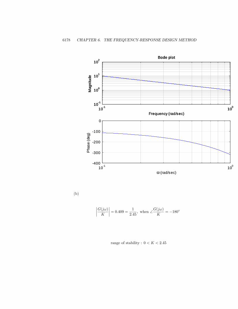
6178 CHAPTER 6. THE FREQUENCY-RESPONSE DESIGN METHOD
101 100101
100
101
102
Frequency (rad/sec)
Mag
nitu
de
Bode plot
101 100101
100
101
102
Frequency (rad/sec)
Mag
nitu
de
Bode plot
101 100400
300
200
100
0
ω (rad/sec)
Pha
se (d
eg)
101 100101
100
101
102
Frequency (rad/sec)
Mag
nitu
de
Bode plot
101 100101
100
101
102
Frequency (rad/sec)
Mag
nitu
de
Bode plot
101 100400
300
200
100
0
ω (rad/sec)
Pha
se (d
eg)
(b)
����G(j!)K
���� = 0:409 = 1
2:45; when \G(j!)
K= �180�
range of stability : 0 < K < 2:45

6179
101 100 101102
101
100
101
ω (rad/sec)
Mag
nitu
de
Bode plot
101 100 101102
101
100
101
ω (rad/sec)
Mag
nitu
de
Bode plot
101 100 101400
300
200
100
0
ω (rad/sec)
Pha
se (d
eg)
101 100 101102
101
100
101
ω (rad/sec)
Mag
nitu
de
Bode plot
101 100 101102
101
100
101
ω (rad/sec)
Mag
nitu
de
Bode plot
101 100 101400
300
200
100
0
ω (rad/sec)
Pha
se (d
eg)
65. In Chapter 5, we used various approximations for the time delay, one ofwhich is the �rst order Padé
e�Tds �= H1(s) =1� Tds=21 + Tds=2
:
Using frequency response methods, the exact time delay
H2(s) = e�Tds:
can be used. Plot the phase of H1(s) and H2(s) and discuss the impli-cations.
Solution :
The approximation H1(j!) and the true phase H2(j!) are compared inthe plot below:

6180 CHAPTER 6. THE FREQUENCY-RESPONSE DESIGN METHOD
101 100 101400
300
200
100
0
Normalized Frequency,ω Td (rad)
Pha
se (d
eg)
Time Delay Phase Lag
H1
H2
101 100 101400
300
200
100
0
Normalized Frequency,ω Td (rad)
Pha
se (d
eg)
Time Delay Phase Lag
101 100 101400
300
200
100
0
Normalized Frequency,ω Td (rad)
Pha
se (d
eg)
Time Delay Phase Lag
H1
H2
101 100 101400
300
200
100
0
Normalized Frequency,ω Td (rad)
Pha
se (d
eg)
Time Delay Phase Lag
H1(j!) closely approximates the correct phase of the delay (phase of
H2(s)) for !Td .�
2and progressively worsens above that frequency. The
implication is that the H1(s) approximation should not be trusted for
crossover frequencies !c &�
2Td. Instead, one should use the exact phase
for the time delay given by H2(s):
66. Consider the heat exchanger of Example 2.15 with the open-loop transferfunction
G(s) =e�5s
(10s+ 1)(60s+ 1):
(a) Design a lead compensator that yields PM � 45� and the maximumpossible closed-loop bandwidth.
(b) Design a PI compensator that yields PM � 45� and the maximumpossible closed-loop bandwidth.
Solution :

6181
101 100101
100
ω (rad/sec)
Mag
nitu
deBode plot with Lead Compensation
101 100101
100
ω (rad/sec)
Mag
nitu
deBode plot with Lead Compensation
101 100200
180
160
140
120
100
ω (rad/sec)
Pha
se (d
eg)
101 100101
100
ω (rad/sec)
Mag
nitu
deBode plot with Lead Compensation
101 100101
100
ω (rad/sec)
Mag
nitu
deBode plot with Lead Compensation
101 100200
180
160
140
120
100
ω (rad/sec)
Pha
se (d
eg)
(a) First, make sure that the phase calculation includes the time delaylag of -Td! = �5!: A convenient placement of the lead zero is at! = 0:1 because that will preserve the -1 slope until the lead pole.We then raise the gain until the speci�ed PM is obtained in order tomaximize the crossover frequency. The resulting lead compensator,
D(s) =90(s+ 0:1)
(s+ 1)
yields PM = 46� as seen by the Bode below.Also note that thecrossover frequency, !c = 0:15 rad/sec, which can be read approxi-mately from the plot above, and veri�ed by using the margin com-mand in Matlab with the phase adjusted by the time delay lag.
(b) The brealpoint of the PI compensator needs to be kept well below 0.1in order to maintain a positive phase margin at as high a crossoverfrequency as possible. In Table 4.1, Zeigler-Nichols suggest a break-

6182 CHAPTER 6. THE FREQUENCY-RESPONSE DESIGN METHOD
point at ! = 1=17, so we will select a PI of the form :
D(s) = K
�1 +
1
20s
�
and select the gain so that the PM speci�cation is met. ForK = 0:55the phase margin is 46� as shown by the Bode below:
102 101102
101
100
101
ω (rad/sec)
Mag
nitu
de
Bode plot with PI compensation
102 101102
101
100
101
ω (rad/sec)
Mag
nitu
de
Bode plot with PI compensation
102 101200
150
100
50
0
ω (rad/sec)
Pha
se (d
eg)
102 101102
101
100
101
ω (rad/sec)
Mag
nitu
de
Bode plot with PI compensation
102 101102
101
100
101
ω (rad/sec)
Mag
nitu
de
Bode plot with PI compensation
102 101200
150
100
50
0
ω (rad/sec)
Pha
se (d
eg)
Note with this compensation that !c = 0:02 rad/sec, which is con-siderably lower than that yielded by the lead compensation.

6183
Figure 6.105: Control system for Problem 67
Problems and Solutions for Section 6.9
67. A feedback control system is shown in Fig.6.105. The closed-loop systemis speci�ed to have an overshoot of less than 30% to a step input.
(a) Determine the corresponding PM speci�cation in the frequency do-main and the corresponding closed-loop resonant peak valueMr. (SeeFig. 6.38)
(b) From Bode plots of the system, determine the maximum value of Kthat satis�es the PM speci�cation.
(c) Plot the data from the Bode plots (adjusted by the K obtained inpart (b)) on a copy of the Nichols chart in Fig. 6.84 and determine theresonant peak magnitude Mr. Compare that with the approximatevalue obtained in part (a).
(d) Use the Nichols chart to determine the resonant peak frequency !rand the closed-loop bandwidth.
Solution :
(a) From Fig. 6.38 :
Mp � 0:3 =) PM � 40o =)Mr � 1:5
resonant peak : Mr � 1:5
(b) A sketch of the asymptotes of the open loop Bode shows that a PMof �= 40o is obtained when K = 8: A Matlab plot of the Bode canbe used to re�ne this and yields
K = 7:81
for PM = 40o:
(c) The Nichols chart below shows that Mr = 1:5 which agrees exactlywith the prediction from Fig. 6.38:

6184 CHAPTER 6. THE FREQUENCY-RESPONSE DESIGN METHOD
(d) The corresponding frequency where the curve is tangent toMr = 1:5is:
!r = 2:41 rad/sec
as can be determined by noting the frequency from the Bode plotthat corresponds to the point on the Nichols chart.The bandwidth !BW is determined by where the curve crosses theclosed-loop magnitude of 0.7 and noting the frequency from the Bodeplot that corresponds to the point on the Nichols chart
!BW = 3:94 rad/sec
68. The Nichols plot of an uncompensated and a compensated system areshown in Fig. 6.106.

6185
Figure 6.106: Nichols plot for Problem 68

6186 CHAPTER 6. THE FREQUENCY-RESPONSE DESIGN METHOD
(a) What are the resonance peaks of each system?(b) What are the PM and GM of each system?(c) What are the bandwidths of each system?(d) What type of compensation is used?
Solution :
(a) Resonant peak :
Uncompensated system : Resonant peak = 1:5 (!r = 50 rad/sec)
Compensated system : Resonant peak = 1::05 (!r = 20 rad/sec)
(b) PM, GM :
Uncompensated system : PM = 42�; GM =1
0:2= 5
Compensated system : PM = 64�; GM =1
0:1= 10
(c) Bandwidth :
Uncompensated system : Bandwidth = 70 rad/sec
Compensated system : Bandwidth = 30 rad/sec
(d) Lag compensation is used, since the bandwidth is reduced.

6187
69. Consider the system shown in Fig. 6.97.
(a) Construct an inverse Nyquist plot of [Y (j!)=E(j!)]�1.
(b) Show how the value of K for neutral stability can be read directlyfrom the inverse Nyquist plot.
(c) For K = 4, 2, and 1, determine the gain and phase margins.
(d) Construct a root-locus plot for the system, and identify correspondingpoints in the two plots. To what damping ratios � do the GM andPM of part (c) correspond?
Solution :
(a) See the inverse Nyquist plot.
(b) Let
G(j!) =Y (j!)
E(j!)
The characteristic equation with s = j! :
1 +KuG(j!) = 0
=) G�1 = �Ku
From the inverse Nyquist plot,
�Ku = �4 =) Ku = 4
(c)K GM PM4 �4
�4 = 1 0�
2 �4�2 = 2 18:3�
1 �4�1 = 4 38:1�

6188 CHAPTER 6. THE FREQUENCY-RESPONSE DESIGN METHOD
(d)K closed-loop poles �
4�4
�j1:73 0
2�3:63
�0:19� j1:27 0:14
1�3:37
�0:31� j0:89 0:33
70. An unstable plant has the transfer function
Y (s)
F (s)=
s+ 1
(s� 1)2 :

6189
A simple control loop is to be closed around it, in the same manner as theblock diagram in Fig. 6.97.
(a) Construct an inverse Nyquist plot of Y=F .
(b) Choose a value of K to provide a PM of 45�. What is the corre-sponding GM?
(c) What can you infer from your plot about the stability of the systemwhen K < 0?
(d) Construct a root-locus plot for the system, and identity correspond-ing points in the two plots. In this case, to what value of � doesPM = 45� correspond?
Solution :
(a) The plots are :
(b) From the inverse Nyquist plot, K = 3:86 provides a phase margin of45�.Since K = 2 gives \G(j!)�1 = 180� ,
GM =2
3:86= 0:518
Note that GM is less than 1, but the system with K = 3:86 is stable.
K = 3:86; GM = 0:518
(c) We can apply stability criteria to the inverse Nyquist plot as follows:

6190 CHAPTER 6. THE FREQUENCY-RESPONSE DESIGN METHOD
Let
N = Net number of clockwise encirclement of �KP = Number of poles of G�1 in RHP
( = Number of zeros of G in RHP)
Z = Number of closed-loop system roots in RHP
Then,
�K < �2 K > 2 =) N = 0; P = 0=) Z = 0 =) Stable
�2 < �K < 1�1 > K > 2 =) N = 2; P = 0
=) Z = 2 =) Two unstable closed-loop roots
�K > 1K < �1 =) N = 1; P = 0
=) Z = 1 =) One unstable closed-loop root
Then, we can infer from the inverse Nyquist plot the stability situa-tion when K is negative. In summary, when K is negative, there areeither one or two unstable roots, and the system is always unstable.
(d) The stability situation seen in the root locus plot agrees with thatobtained from the inverse Nyquist plot.They show :
K > 2 Stable�1 < K < 2 Two unstable closed-loop rootsK < �1 One unstable closed-loop root
For the phase margin 45�,
closed-loop roots = �0:932� 1:999j� = 0:423

6191
Figure 6.107: Control system for Problem 71
71. Consider the system shown in Fig. 6.107(a).
(a) Construct a Bode plot for the system.
(b) Use your Bode plot to sketch an inverse Nyquist plot.
(c) Consider closing a control loop aroundG(s), as shown in Fig. 6.107(b).Using the inverse Nyquist plot as a guide, read from your Bode plotthe values of GM and PM when K = 0:7, 1.0, 1.4, and 2. What valueof K yields PM = 30�?
(d) Construct a root-locus plot, and label the same values of K on thelocus. To what value of � does each pair of PM/GM values corre-spond? Compare the � vs PM with the rough approximation in Fig.6.37
Solution :
(a) The �gure follows :

6192 CHAPTER 6. THE FREQUENCY-RESPONSE DESIGN METHOD
101 100 101 102
105
100
ω (rad/sec)
Mag
nitu
de
Bode Diagrams
101 100 101 102300
250
200
150
100
50
ω (rad/sec)
Pha
se (d
eg)
101 100 101 102
105
100
ω (rad/sec)
Mag
nitu
de
Bode Diagrams
101 100 101 102300
250
200
150
100
50
ω (rad/sec)
Pha
se (d
eg)
(b) The �gure follows :

6193
(c)
K GM PM
K = 0:7 5:71 (! = 2:00) 54:7� (!c = 0:64)K = 1 4:00 (! = 2:00) 44:1� (!c = 0:85)K = 1:4 2:86 (! = 2:00) 33:1� (!c = 1:08)K = 2 2:00 (! = 2:00) 21:4� (!c = 1:36)For PM = 30�
K = 1:542:60 (! = 2:00) 30:0� (!c = 1:15)

6194 CHAPTER 6. THE FREQUENCY-RESPONSE DESIGN METHOD
(d)K closed-loop roots �
K = 0:7�2:97
�0:51� 0:82j 0:53
K = 1�3:13
�0:43� 1:04j 0:38
K = 1:4�3:30
�0:35� 1:25j 0:27
K = 2�3:51
�0:25� 1:49j 0:16

Chapter 7
State-Space Design
Problems and Solutions for Section 7.3: Block diagrams andState Space
1. Write the dynamic equations describing the circuit in Fig. 7.82. Write the equations as a second-order di¤erential equation in y(t). Assuming a zero input, solve the di¤erential equation for y(t)using Laplace-transform methods for the parameter values and initial conditions shown in the�gure. Verify your answer using the initial command in Matlab.
Solution:
i = Cdy
dt(1)
v = Ldi
dt(2)
u(t)� Ldidt�Ri(t)� y(t) = 0
di
dt=u
L� R
Li� 1
Cy (3)
Figure 7.82: Circuit for Problem 7.1
7001

7002 CHAPTER 7. STATE-SPACE DESIGN
Substituting the given values for L, R, and C we have for equation (3):
di
dt= u� 2dy
dt� y
�y + 2 _y + y = u
Characteristic equation:
s2 + 2s+ 1 = 0
(s+ 1)2 = 0
So:y(t) = A1e
�t +A2te�t
Solving for the coe¢ cients:
y(t) = A1e�t +A2te
�t
y(t0) = A1e�t0 +A2t0e
t0 = 1
_y(t) = �A1e�t +A2e�t �A2te�t
_y(t0) = �A1e�t0 +A2e�t0 �A2te�t0 = 0
) A2 = et0 and A1 = (1� t0)et0
y(t) = (1� t0)et0�t + tet0�t:
To verify the solution using Matlab, re-write the di¤erential equation in state space form,� :y::y
�=
�0 1�1 �2
� �y:y
�+
�1L0
�u = ax+ bu
y =�1 0
� � y:y
�= cx,
where x = [y:y]T . Then the following Matlab statements,
a=[0,1;-1,-2];
b=[0;1];
c=[1,0];
d=[0];
sys=ss(a,b,c,d);
xo=[1;0];
[y,t,x]=initial(sys,xo);
plot(t,y);
grid;
xlabel(�Time (sec)�);
ylabel(�y(t)�);
title(�Initial condition response�);
generate the initial condition response shown below that agrees with the analytical solutionabove.

7003
0 2 4 6 8 100
0.1
0.2
0.3
0.4
0.5
0.6
0.7
0.8
0.9
1
Time (sec)
y(t)
Initial condition response
0 2 4 6 8 100
0.1
0.2
0.3
0.4
0.5
0.6
0.7
0.8
0.9
1
Time (sec)
y(t)
Initial condition response
Problem 7.1: Initial condition response.
2. A schematic for the satellite and scienti�c probe for the Gravity Probe-B (GP-B) experimentthat was launched on April 30, 2004 is sketched in Fig. 7.83. Assume that the mass of thespacecraft plus helium tank, m1, is 2000 kg and the mass of the probe, m2, is 1000 kg. Arotor will �oat inside the probe and will be forced to follow the probe with a capacitive forcingmechanism. The spring constant of the coupling, k, is 3:2 � 106. The viscous damping b is4:6� 103:
(a) Write the equations of motion for the system consisting of masses m1 and m2 using theinertial position variables, y1 and y2.
(b) The actual disturbance u is a micrometeorite, and the resulting motion is very smallTherefore, rewrite your equations with the scaled variables z1 = 106y1, z2 = 106y2, andv = 1000u:
(c) Put the equations in state-variable form using the state x = [z1 _z1 z2 _z2]T ; the output
y = z2; and the input an impulse, u = 10�3�(t) N� sec on mass m1:
(d) Using the numerical values, enter the equations of motion into Matlab in the form
_x = Fx+Gv (1)
y = Hx+ Jv (2)

7004 CHAPTER 7. STATE-SPACE DESIGN
and de�ne the Matlab system: sysGPB = ss(F,G,H,J). Plot the response of y caused bythe impulse with the Matlab command impulse(sysGPB). This is the signal the rotor mustfollow.
(e) Use the Matlab commands p = eig(F) to �nd the poles (or roots) of the system and z =tzero(F,G,H, J) to �nd the zeros of the system.
m 1 m 2
y 1
y 2
R o t o rk
u
b
Figure 7.83: Schematic diagram of the GP-B satellite and probe.
Solution:(a) The rotor is not part of the problem and can be ignored in writing the equations ofmotion
m1�y1 = u� k (y1 � y2)� b ( _y1 � _y2)
m2�y2 = �k (y2 � y1)� b ( _y2 � _y1)
(b) Let�s put in the values for the parameters as well as scale the variables as requested.
2000�10�6�z1
�=
1
1000v � 10�6(3:2� 106) (z1 � z2)� 10�6(4:6� 103) ( _z1 � _z2)
1000�10�6�z2
�= �10�6(3:2� 106) (z2 � z1)� 10�6(4:6� 103) ( _z2 � _z1)
which becomes
�z1 = �(1:6� 103) (z1 � z2)� (2:3) ( _z1 � _z2) +1
2v
�z2 = �(3:2� 103) (z2 � z1)� (4:6) ( _z2 � _z1)
(c) The state-variable form for x = [z1 _z1 z2 _z2]T is
_x1 = x2
_x2 = �(1:6� 103) (x1 � x3)� (2:3) (x2 � x4) +1
2v
_x3 = x4
_x4 = �(3:2� 103) (x3 � x1)� (4:6) (x4 � x2)
or, in matrix form2664_x1_x2_x3_x4
3775 =2664
0 1 0 0�1:6� 103 �2:3 1:6� 103 2:3
0 0 0 13:2� 103 4:6 �3:2� 103 �4:6
37752664x1x2x3x4
3775+266401200
3775 v

7005
and the output equation is
y = [0 0 1 0]
2664x1x2x3x4
3775+ 0
(d) The system matrices
F =
26640 1 0 0
�1:6� 103 �2:3 1:6� 103 2:30 0 0 1
3:2� 103 4:6 �3:2� 103 �4:6
3775
G =
266401200
3775 and H = [0 0 1 0] and J = 0
plus the Matlab statements:
sysGPB = ss(F,G,H,J);
t=0:0.001:1;
y=impulse(sysGPB,t); % u = 10�3 implies that v = 1
plot(t,y)
produce the plot below.

7006 CHAPTER 7. STATE-SPACE DESIGN
0 0.2 0.4 0.6 0.8 10
0.05
0.1
0.15
0.2
0.25
0.3
0.35
Time (sec)
y 2 (mic
rom
eter
s)
impulse response of y2
0 0.2 0.4 0.6 0.8 10
0.05
0.1
0.15
0.2
0.25
0.3
0.35
Time (sec)
y 2 (mic
rom
eter
s)
impulse response of y2
Impulse response for Problem 7.2.
The micro meteorite hits the �rst mass and imparts a velocity of 0:33�m/sec to the twomass system. It also excites the resonant mode of relative motion between the masses thatdies out in less than a second.Problems and Solutions for Section 7.4: Analysis of theState Equations
3. Give the state description matrices in control-canonical form for the following transfer functions:
(a)1
4s+ 1
(b)5(s=2 + 1)
(s=10 + 1)
(c)2s+ 1
s2 + 3s+ 2
(d)s+ 3
s(s2 + 2s+ 2)
(e)(s+ 10)(s2 + s+ 25)
s2(s+ 3)(s2 + s+ 36)Solution:

7007
(a) F = �0:25; G = 1; H = 0:25; J = 0.
(b) F = �10; G = 1; H = �200; J = 25:Hint: Do a partial fraction expansion to �nd the J term �rst.
(c)
F =
��3 �21 0
�; G =
�10
�; H =
�2 1
�; J = [0]:
(d)
F =
24 �2 �2 01 0 00 1 0
35 ; G =
24 100
35 ; H =�0 1 3
�; J = [0]:
(e)
F =
266664�4 �39 �108 0 01 0 0 0 00 1 0 0 00 0 1 0 00 0 0 1 0
377775 ; G =
26666410000
377775 ; H =�0 1 11 35 250
�; J = [0]:
4. Use the Matlab function tf2ss to obtain the state matrices called for Problem 7.3.
Solution:
In all cases, simply form num and den given below and then use the Matlab command [F,G,H,J]= tf2ss(num,den).
(a) num =�0 1
�, den =
�4 1
�:
(b) num =�5=2 5
�, den =
�1=10 1
�.
(c) num =�0 2 1
�; den =
�1 3 2
�:
(d) num =�0 0 1 3
�; den =
�1 2 2 0
�:
(e) num =�0 0 1 11 35 250
�; den =
�1 4 1 39 108 0 0
�.
Note that the answers are the same as for Problem 7.2.
Hint: The Matlab function conv will save time when forming the numerator and denominatorfor part (e).
5. Give the state description matrices in normal-mode form for the transfer functions of Prob-lem 7.3. Make sure that all entries in the state matrices are realvalued by keeping any pairs ofcomplex conjugate poles together, and realize them as a separate subblock in control canoni-cal form.
Solution:
(a) F = �0:25; G = 1; H = 0:25; J = 0:
(b) F = �10; G = 1; H = �200; J = 25:(c)
2s+ 1
s2 + 3s+ 2=
2s+ 1
(s+ 1)(s+ 2)=
�1s+ 1
+3
s+ 2;
The computation can also be done using the residue command in Matlab.

7008 CHAPTER 7. STATE-SPACE DESIGN
Block diagram for Problem 7.5 (c).
F =
��1 00 �2
�; G =
�11
�; H =
��1 3
�; J = [0]:
(d)s+ 3
s(s2 + 2s+ 2)=3=2
s� 3=2s+ 2
s2 + 2s+ 2;
The computation can also be done using the residue command in Matlab.
Block diagram for Problem 7.5 (d).
F =
24 0 0 00 �2 �20 1 0
35 ; G =
24 110
35 ; H =�32 � 3
2 �2�; J = [0]:
(e) The hard part is getting the expansion,
(s+ 10)(s2 + s+ 25)
s2(s+ 3)(s2 + s+ 36)=�0:5118s+ 2:3148
s2+0:57407
s+ 3+�0:0622s+ 0:3452
s2 + s+ 36
You can use the Matlab function residue to obtain this. From the �gure, we have,

7009
Block diagram for Problem 7.5 (e).
F =
2666640 0 0 0 01 0 0 0 00 0 �3 0 00 0 0 �1 �360 0 0 1 0
377775 ; G =
26666410110
377775 ; H =��0:5118 2:3148 0:57407 �0:0622 0:3452
�; J = [0]:
6. A certain system with state x is described by the state matrices,
F =
��2 1�2 0
�; G =
�13
�;
H = [ 1 0 ]; J = 0:
Find the transformation T so that if x = Tz, the state matrices describing the dynamics of zare in control canonical form. Compute the new matrices A, B, C, and D.
Solution:
Following the procedure outlined in the chapter, we have,
C =�G FG
�=
�1 13 �2
�:
t2 =�0 1
�C�1 = 1
5
�3 �1
�;
t1 = t2F =1
5
��4 3
�:

7010 CHAPTER 7. STATE-SPACE DESIGN
Thus,
T�1 =
��4=5 3=53=5 �1=5
�=) T =
�1 33 4
�;
A = T�1FT =
��2 �21 0
�; B = T�1G =
�10
�;
C = HT =�1 3
�; D = J = 0:
7. Show that the transfer function is not changed by a linear transformation of state.
Solution:
Assume the original system is,
_x = Fx+Gu;
y = Hx+ Ju;
G(s) = H(sI� F)�1G+ J:
Assume a change of state from x to z using the nonsingular transformation T;
x = Tz:
The new system matrices are,
A = T�1FT; B = T�1G; C = HT; D = J:
The transfer function is,
Gz(s) = C(sI�A)�1B+D= HT(sI�T�1FT)�1T�1G+ J:
If we factor T on the left and T�1 on the right of the (sI�T�1FT)�1 term, we obtain,
Gz(s) = HT(sTT�1 �T�1FT)�1T�1G+ J
= HTT�1(sI� F)�1TT�1G+ J = H(sI� F)�1G+ J = G(s):
8. Use block-diagram reduction or Mason�s rule to �nd the transfer function for the system inobserver canonical form depicted by Fig. 7.31.
Solution:
(a) We will show the process for the general third-order case shown below. Combine the feed-forward terms to produce the top �gure on the next page. Then, reduce the last loop to getthe �gure on the bottom.

7011
Problem 7.8: Observer canonical form.
Observer canonical form: feedforward terms combined.
Observer canonical form: one loop reduced.
(a) Using Mason�s rule:Forward path gains:

7012 CHAPTER 7. STATE-SPACE DESIGN
p1 =b3s3; p2 =
b2s2; p3 =
b1s
Loop path gains:`1 = �
a3s3; `2 = �
a2s2; `3 = �
a1s
Y
R=
p1 + p2 + p31� `1 � `2 � `3
=b3s3 +
b2s2 +
b1s
1 + a3s3 +
a2s2 +
a1s
=b1s
2 + b2s+ b3s3 + a1s2 + a2s+ a3
:
9. Suppose we are given a system with state matrices F;G; H (J = 0 in this case). Find thetransformation T so that, under Eqs. (7.24) and (7.25), the new state description matrices willbe in observer canonical form.
Solution:
Express the transformation matrix in terms of its column vectors,
T = [t1 t2 t3]
Then if A is in observer canonical form,
TAo = [� t1 t2] = FT = [Ft1 Ft2 Ft3]
Co =�1 0 0
�= HT = [Ht1 Ht2 Ht3]:
From these,24 HHFHF2
35 t3 =24 001
35 =) t3 = O�1�0 0 1
�T; t2 = Ft3; t1 = Ft2:
10. Use the transformation matrix in Eq. (7.41) to explicitly multiply out the equations at the endof Example 7.10.
Solution:
Am = T�1AcT =
�1 31 4
� ��7 �121 0
� �4 �3�1 1
�=
��4 00 �3
�:
Bm = T�1Bc =
�1 31 4
� �10
�=
�11
�:
Cm = CcT =�1 2
� � 4 �3�1 1
�=�2 �1
�:
11. Find the state transformation that takes the observer canonical form of Eq. (7.35) to the modalcanonical form.
Solution:
We wish to �nd the transformation T such that,
Am = T�1AoT = diag(�1; �2; :::; �n):

7013
Bm = T�1Bo;
Cm = CoT:
The columns of T are the eigenvectors of Ao. The eigenvectors of Ao are all of the form (whichcan be proved by induction):
ti =
266666664
1�i + a1
�2i + a1�i + a2�3i + a1�
2i + a2�i + a3...
�n�1i + a1�n�2i + a2�
n�3i + : : :+ an�1
377777775; i = 1; 2; :::; n:
T =�t1 t2 ::: tn
�:
For the cases where there are repeated eigenvalues, and a full set of linearly independent eigen-vectors do not exist, then the generalized eigenvectors need to be computed to transform thesystem to Jordan form (see Strang, 1988).
12. a) Find the transformation T that will keep the description of the tape-drive system of Ex-ample 7.11 in modal canonical form but will convert each element of the input matrix Bm tounity.
b) Use Matlab to verify that your transformation does the job.
Solution:
(a) We would like to �nd a transformation matrix T1such that,
Bm = T�11 G =
�1 1 1 1 1
�T:
Since T1 is full rank, this is equivalent to solving G = T1Bm. Recall that the magnitude ofthe eigenvectors are can be scaled by any arbitrary constant, so long as the direction in statespace is preserved. Thus we can scale each of the eigenvectors of T found in Example 7.3 andkeep the solution in modal form. Let,
T1 = TN = [n1t1 n2t2 � � �n5t5];
where ti are the eigenvectors, ni are scalars and N=diag(n1,� � � ,n5). Now,
G = T1Bm= TNBm= Tn;) n = T�1G;
and n = [n1 n2 � � �n5]T . Thus, to �nd the transformation T1, we compute n and multiply toget T1= TN = Tdiag(n1 n2 � � �n5):

7014 CHAPTER 7. STATE-SPACE DESIGN
(b) In Matlab,
T =
2666641:4708 �0:17221 �1:4708 �1:5432 �3:32370:7377 2:8933 �0:7377 �2:9037 �0:1282�0:7376 �5:4133 0:6767 �1:3533 �4:05990:9227 �6:5022 �0:9227 �2:7962 �9:9016�0:0014 0:1663 0:0014 0:0449 3:9341
377775 ;n = TnG;N = diag(n);
T1 = T � N;
T1 =
266664�0:3883 0:0247 2:8708 �4:8234 2:3162�0:0897 �0:0129 0:0000 1:2239 �1:12142:9239 0:0000 2:8708 �8:2970 2:5023�0:9314 0:0376 0:0000 2:1053 �1:21150:0133 0:0001 �0:0000 �0:0745 1:0612
377775 ;Bm = T1nG =
�1 1 1 1 1
�T;
Am = T1nF � T1 =
266664�0:6371 0:0257 �0:0000 0:0000 �0:0000�17:2941 �0:6371 0:0000 �0:0000 �0:0000�0:0000 0:0000 �0:0000 0:0000 �0:0000�0:0000 0:0000 0:0000 �0:5075 �0:0000�0:0000 0:0000 0:0000 0:0000 �0:9683
377775 :
13. a) Find the state transformation that will keep the description of the tape-drive system ofExample 7.11 in modal canonical form but will cause the poles to be displayed in Am in orderof increasing magnitude.b) Use Matlab to verify your result in part (a), and give the complete new set of state matricesas A, B, C, and D.
Solution:
(a) To change the order of the eigenvalues (poles), pi, in Am, all we need to do is re-order theeigenvectors in T . In this case, jp5j > jp1j = jp2j > jp4j > jp3j: Thus, T2 = [t5 t1 t2 t4 t3].
(b) Our solution uses the Matlab sort command to re-order eigenvectors. Note that thisapproach is independent of the size of the system matrix Am. T is the same as in Problem 7.10.Because of the equality of the magnitudes of the complex eigenvectors, we can switch two of thecolumns of the matrix T2. In Matlab,
p = eig(F);
[f, indices] = sort(abs(p));
T2 = T(:,indices);
n = T2nG;
T3 = T2*diag(n);

7015
Am2 = T3nF*T3;
Am2 =
266664�0:0000 0:0000 �0:0000 0:0000 �0:00000:0000 �0:5075 �0:0000 0:0000 �0:0000�0:0000 0:0000 �0:6371 0:0257 �0:00000:0000 0:0000 �17:2941 �0:6371 �0:00000:0000 0:0000 �0:0000 0:0000 �0:9683
377775 ;
Bm2 = T3nG;Bm2 = [1 1 1 1 1]T
Cm2 = h3*T3;
Cm2 =�2:8708 �6:5602 1:2678 0:0123 2:4092
�,
Dm2 = 0;
14. Find the characteristic equation for the modal-form matrix Am of Eq. (7.17a) using Eq. (7.58).
Solution:
det(sI� F) = det�s+ 4 00 s+ 3
�= (s+ 4)(s+ 3)
Since Am was already in modal form, your solution is easily checked by inspection.
15. Given the system,
_x =
��4 1�2 �1
�x+
�01
�u;
with zero initial conditions, �nd the steady-state value of x for a step input u.
Solution:
We are given _x = Fx +Gu. Steady-state means that _x = 0 and a step input (or unit step)means u = 1(t). Thus, assuming that F is invertible (which you can check), we have,
0 = Fxss +G =) xss = �F�1G =
��4 1�2 �1
��1 �01
�=
�1=62=3
�:
This can be veri�ed in Matlab with step(F,G,H,J,1) where H=eye(size(F)) and J=[0;0].
16. Consider the system shown in Fig. 7.83.
U S
2
1
G 1 5s 1 41 G 2 52 s
1
H 2 5s1 H 1 5s
1x 2x 3
x 4
S
1
1
S
1
1
Yx 1
Figure 7.84: A block diagram for Problem 7.16.

7016 CHAPTER 7. STATE-SPACE DESIGN
a) Find the transfer function from U to Y .b) Write state equations for the system using the state variables indicated.
Solution:
(a) The system is equivalent to the block diagram shown. Following the block diagram back toknown state variables,
y = x1
�1 + 2s+
1
s
�;
and,
x1 =1
2s(s+ 4)
�u� 1
s
�2s+
1
s
�x1
�;
resulting in,Y (s)
U(s)=
2s3 + s2 + s
2s4 + 8s3 + 2s2 + 1:
Block diagram for solution of Problem 7.16 (a).
Another possible solution is in terms of Mason�s rule.
(b) 2664_x1_x2_x3_x4
3775 =
26640 0 0 1
21 0 0 00 1 0 00 0 �1 �4
37752664x1x2x3x4
3775+26640001
3775u;y =
�1 1 0 1
�x:
With practice, you should be able to see quickly that _x3 is simply the input to block H2, whichis the sum of x2 and x4. But this is nothing more than the third row of the matrix equationabove. Your results can be checked for consistency using Matlab�s command ss2tf.
17. Using the indicated state variables, write the state equations for each of the systems shown inFig. 7.85. Find the transfer function for each system using both block-diagram manipulationand matrix algebra [as in Eq. (7.48)].
Solution:
(a) Performing a partial fraction expansion on (s + 2)=(s + 4), Fig. 7.85(a) can be redrawn asshown below.

7017
U s1S
1
1
s 1 41
s 1 3s 1 2
s 1 1 01
s 1 21
s4
5
YSx 1x 2
x 3
x 1
U S1
1
YSx 3
x 4
s 1 31
1
1
x 1x 2
( a )
( b )
1
12
2
Figure 7.85: Block diagrams for Problem 7.17.
Redrawn block diagram for solution to Problem 7.17(a).
By inspection of the block diagram, the state equations are,
_x =
24 �5 1 10 �3 �20 0 �4
35x+24 011
35u;y =
�1 0 1
�x:
Computing G(s) = H(sI� F)�1G, the following transfer function is obtained:
Y (s)
U(s)=
s2 + 10s+ 20
s3 + 12s2 + 47s+ 60:
We can use the Matlab ss2tf command to verify this result.
(b) Using the second block diagram given in Fig. 7.85(b), we can write,
_x =
2664�3 1 0 00 0 4 00 �1 �2 10 0 0 �10
3775x+26640011
3775u;y =
�1 0 1 0
�x:

7018 CHAPTER 7. STATE-SPACE DESIGN
Computing H(sI� F)�1G (using Matlab�s ss2tf), we obtain the following transfer function,
Y (s)
U(s)=
s3 + 14s2 + 37s+ 44
s4 + 15s3 + 60s2 + 112s+ 120:
18. For each of the listed transfer functions, write the state equations in both control and observercanonical form. In each case draw a block diagram and give the appropriate expressions for F,G, and H.
a)s2 � 2
s2(s2 � 1) (control of an inverted pendulum by a force on the cart)
b)3s+ 4
s2 + 2s+ 2
Solution:
(a)
Y (s)
U(s)=
s2 � 2s2(s2 � 1) :
This transfer function can be realized in controller canonical form as shown below. From the�gure, we have,
2664_x1_x2_x3_x4
3775 =
26640 1 0 01 0 0 00 1 0 00 0 1 0
37752664x1x2x3x4
3775+26641000
3775u;y =
�0 1 0 �2
�x:
Controller canonical form for the transfer function of Problem 7.18(a).
The block diagram for observer canonical form is shown below. From the �gure, we have,2664_x1_x2_x3_x4
3775 =
26640 1 0 01 0 1 00 0 0 10 0 0 0
37752664x1x2x3x4
3775+2664
010�2
3775u;y =
�1 0 0 0
�x:

7019
Observer canonical form for the transfer function of Problem 7.18(a).
(b)
Y (s)
U(s)=
3s+ 4
s2 + 2s+ 2:
This transfer function can be realized in Controller canonical form as shown below. From the�gure, we have,
�_x1_x2
�=
��2 �21 0
� �x1x2
�+
�10
�u;
y =�3 4
�x:
Controller canonical form for the transfer function of Problem 7.18(b).
The block diagram for observer canonical form is shown below. From the �gure, we have:
�_x1_x2
�=
��2 1�2 0
� �x1x2
�+
�34
�u;
y =�1 0
�x:

7020 CHAPTER 7. STATE-SPACE DESIGN
18:pdf
Observer canonical form for the transfer function of Problem 7.18(b).
19. Consider the transfer function, G(s) = Y (s)U(s) =
s+1s2+5s+6 : (7.263)
a) By rewriting Eq. (7.263) in the form,
G(s) =1
s+ 3
�s+ 1
s+ 2
�;
�nd a series realization of G(s) as a cascade of two �rst-order systems.b) Using a partial-fraction expansion of G(s), �nd a parallel realization of G(s).c) Realize G(s) in control canonical form.
Solution:
(a) The series realization shown below is given by:
G(s) =
�1
s+ 3
��s+ 1
s+ 2
�= g2(s)g1(s):
Series connection of G(s) for Problem 7.19(a).
For g1(s); _x1 = �2x1 + u1; y1 = �x1 + u1:For g2(s); _x2 = �3x2 + u2; y2 = x2:
The series interconnections result in u = u1; y = y2; u2 = y1. Therefore,�_x1_x2
�=
��2 0�1 �3
� �x1x2
�+
�11
�u;
y =�0 1
�x:

7021
The Matlab command series can also be used.
(b) The parallel realization, shown below, is given by:
G(s) =2
s+ 3+
�1s+ 2
= g1(s) + g2(s):
Parallel connection of G(s) for Problem 7.19(b).
For g1(s); _x1 = �3x1 + u1; y1 = 2x1:For g2(s); _x2 = �2x2 + u2; y2 = �x2:
The interconnections are u1 = u2 = u; y = y1 + y2. Therefore,�_x1_x2
�=
��3 00 �2
� �x1x2
�+
�11
�u;
y =�2 �1
�x:
The Matlab command parallel can also be used.
(c) Control canonical form, shown in Fig. 7.17, is realized by simply picking o¤ the appropriatecoe¢ cients of the original (strictly proper) transfer function. If the original function is notstrictly proper, then it should be reduced to a feedthrough term plus a strictly proper term.
Controller canonical form of G(s) for Problem 7.19(c).
For G(s), we have,
F =
��5 �61 0
�; G =
�10
�; H =
�1 1
�:
Problems and Solutions for Section 7.5: Control-Law De-sign for Full-State Feedback

7022 CHAPTER 7. STATE-SPACE DESIGN
20. Consider the plant described by,
_x =
�0 17 �4
�x+
�12
�u;
y = [ 1 3 ]x:
a) Draw a block diagram for the plant with one integrator for each state variable.b) Find the transfer function using matrix algebra.c) Find the closed-loop characteristic equation if the feedback is
(1) u = �[ K1 K2 ]x; (2) u = �Ky.
Solution:
State realization showing integrators explicitly.
(a) See �gure.
(b) Using the formula G(s) = H(sI� F)�1G, we obtain,
G(s) =Y (s)
U(s)=
7s+ 27
s2 + 4s� 7 :
The Matlab command ss2tf can also be used.
(c)
(i) State feedback, u = �[K1 K2]x.
det(�I� F+GK) = det
��+K1 �1 +K2
�7 + 2K2 �+ 4 + 2K2
�= �2 + �(4 + 2K2 +K1) + (6K1 + 7K2 � 7) = 0:
(ii) Output feedback,
u = �Ky = �K�1 3
�x = �
�K 3K
�x:
This yields the following closed-loop characteristic equation:
�2 + �(7K + 4) + (27K � 7) = 0:

7023
Hints: If you have already solved the case for state feedback, simply plug K1 = K and K2 = 3Kinto the characteristic equation for state feedback and �nd the characteristic equation for outputfeedback. The output vector H �xes the ratio among the state variables. Secondly, althoughthere were products of K1 and K2 when we were forming the determinant, they should all cancelin your �nal answer. The reason for this is that the characteristic equation _x = (F�GK)x islinear in K.
21. For the system,
_x =
�0 1
�6 �5
�x+
�01
�u;
y =�1 0
�x;
design a state feedback controller that satis�es the following speci�cations:
� Closed-loop poles have a damping coe¢ cient � = 0:707.
� Step-response peak time is under 3.14 sec.
Verify your design with Matlab.
Solution:
For a second-order system, the speci�cation on rise time can be translated into a value of !nbythe equation !d = �. Then determine !n from !d = !n
p1� �2. This yields !n = 1:414.
Using full state feedback, we would like the a characteristic equation to be,
s2 + 2�!ns+ !2n = s2 + 2s+ 2 = 0:
Using state feedback u = �Kx, we get,
_x = (F�GK)x =�
0 1�6� k1 �5� k2
�x:
Hence the closed-loop characteristic equation is,
s2 + (5 + k2)s+ (6 + k1) = 0:
Comparing coe¢ cients, k1 = �4 and k2 = �3. The Matlab command place can also be used.The reference step can be simulated in Matlab with u = �Kx+ r, and the Matlab commandstep, as shown below.

7024 CHAPTER 7. STATE-SPACE DESIGN
0 1 2 3 4 5 60
0.1
0.2
0.3
0.4
0.5
0.6
0.7
Step Response
Time (sec)
Ampl
itude
0 1 2 3 4 5 60
0.1
0.2
0.3
0.4
0.5
0.6
0.7
Step response for Problem 7.21.
22. a) Design a state feedback controller for the following system so that the closed-loop step responsehas an overshoot of less than 25% and a 1% settling time under 0.115 sec.:
_x =
�0 10 �10
�x+
�01
�u;
y =�1 0
�x:
b) Use the step command in Matlab to verify that your design meets the speci�cations. If itdoes not, modify your feedback gains accordingly.
Solution:
(a) For the overshoot speci�cation,
Mp = e���p1��2 < 25% =) � �= 0:4:
For the 1% settling time speci�cation, we use,
e��!nts = 0:01 =) !n =4:6
�ts:

7025
(b) This can be implemented in Matlab with the following code:
F = [0,1;0,-10];
G = [0;1];
H = [1,0];
J = 0;
zeta = 0.404; % Tweak values slightly so that specs are met.
ts = 0.114;
wn = 4.6/(ts*zeta);
p = roots([1, 2*zeta*wn, wn^2]);
k = place(F,G,p);
sysCL=ss(F-G*k,G,H,J)
step(sysCL);
The step response is shown next.
0 0.02 0.04 0.06 0.08 0.1 0.12 0.140
0.2
0.4
0.6
0.8
1
1.2
1.4x 10 4 Control design with overshoot and settling time specs
Time (sec)
y(t)
0 0.02 0.04 0.06 0.08 0.1 0.12 0.140
0.2
0.4
0.6
0.8
1
1.2
1.4x 10 4 Control design with overshoot and settling time specs
Time (sec)
y(t)
Step response for Problem 7.22.

7026 CHAPTER 7. STATE-SPACE DESIGN
23. Consider the system,
_x =
24 �1 �2 �20 �1 11 0 �1
35x+24 201
35u;y =
�1 0 0
�x:
a) Design a state feedback controller for the system so that the closed-loop step response has anovershoot of less than 5% and a 1% settling time under 4.6 sec.b) Use the step command in Matlab to verify that your design meets the speci�cations. If itdoes not, modify your feedback gains accordingly.
Solution:
(a) There are many di¤erent approaches to designing the control law. We will attack the problemusing a symmetric root locus. We assume the output is x1. Although the system is third-order,we can still use the second-order order rules of thumb in order to get an estimate of where wewould like the closed loop poles.
� =4:6
ts=) �!n = 1;
Mp � 5% =) � > 0:7:
The open-loop poles are at �1:45 and �0:77� j1:47 and the open-loop zeros are at �1:37 and0:37. The symmetric root locus is shown on the next page and was generated using the followingMatlab code:
%%%%%%%%%%%%%%%%%%%%%%%%%%%%%%%%%%%%%%%
% the function srl is used to compute the roots of the symmetric root locus
function [k,p]=srl(f,g,h)
a=[f 0*f;-h�*h -f�];
b=[g;0*g];
c=[0*h g�];
rlocus(a,b,c,0);
[k,p]=rloc�nd(a,b,c,0)
Note that crosses indicate where the closed-loop pole locations have been selected, which roughlycorrespond to the � and !n suggested by the rules of thumb for a second-order system withno zeros. The control gains K =
�0:78 0:07 0:28
�correspond to these closed loop pole
locations. The Matlab command place can be used to verify this computation. The stepresponse is shown next using the Matlab step command.
Technically, this closed-loop step response meets the 4:6 sec 1% settling time and 5% overshoot.However, the right half plane zero close to the origin gives catastrophic results in terms ofundershoot. This should alert the reader to the importance of paying attention to the zeros ofthe system, especially in the right half plane.

7027
4 3 2 1 0 1 2 3 42
1.5
1
0.5
0
0.5
1
1.5
2
Root Locus
Real Axis
Imag
inar
y Ax
is
Symmetric root locus for Problem 7.23.

7028 CHAPTER 7. STATE-SPACE DESIGN
0 0.5 1 1.5 2 2.5 3 3.5 4 4.51
0.8
0.6
0.4
0.2
0
0.2
0.4
0.6
0.8
1
Time (sec)
y(t)
Control design with overshoot and settling time specs
0 0.5 1 1.5 2 2.5 3 3.5 4 4.51
0.8
0.6
0.4
0.2
0
0.2
0.4
0.6
0.8
1
Time (sec)
y(t)
Control design with overshoot and settling time specs
Closed-loop step response for Problem 7.23.
24. Consider the system in Fig. 7.83.
s 2 1 4s
U Y
Figure 7.86: System for Problem 7.24.
a) Write a set of equations that describes this system in the control canonical form as _x =Fx+Gu and y = Hx.b) Design a control law of the form,
u = �[ K1 K2 ]
�x1x2
�;
that will place the closed-loop poles at s = �2� 2j:
Solution:
(a) Let�s write this system in the control canonical form,

7029
�_x1_x2
�=
�0 �41 0
� �x1x2
�+
�10
�u;
y =�1 0
�x:
(b) If u = �[K1 K2]x, the poles of the closed-loop system satisfy det(sI�F+GK) = 0. Thus,
det
�s+K1 �1 +K2
4 s
�= 0 =) s2 +K1s+ 4 +K2 = 0:
The closed-loop characteristic equation is,
(s+ 2� 2j)(s+ 2 + 2j) = s2 + 4s+ 8 = 0:
Comparing coe¢ cients, we have K1 = 4 and K2 = 4. The Matlab command place can also beused to verify this result.
25. Output Controllability : In many situations a control engineer may be interested in controllingthe output y rather than the state x. A system is said to be output controllable if at any timeyou are able to transfer the output from zero to any desired output y� in a �nite time using anappropriate control signal u�. Derive necessary and su¢ cient conditions for a continuous system(F,G,H) to be output controllable. Are output and state controllability related? If so, how?
Solution:
Because we are considering linear systems, if you can take the state from some initial state tosome �nal condition in a �nite time with a �nite input, then you can also take it to the samestate in in�nitesimal time using impulsive inputs. To express this mathematically, let u be,
u(t) = g1�(t) + g2�(1)(t) + � � �+ gn�(n�1)(t);
where �(t) represents a delta function, �(1)(t) represents the �rst derivative of a delta function(a unit doublet), etc., and the gi are scalars to be determined. Let,
u� = [g1 g2 � � � gn]T ;
thenx(0+)� x(0�) = C u�:
Hence, we have found a control signal that will drive the state to arbitrary values given thenon-singularity of the controllability matrix, C.In fact, the invertibility of C is a necessary and su¢ cient condition for state controllability. Foroutput controllability,
Hx(0+)�Hx(0�) = HC u�;y(0+)� y(0�) = HC u�:
Assuming (without loss of generality) that y(0�) = 0, we have,
y(0+) = [HG HFG � � �HFn�1G]u�:

7030 CHAPTER 7. STATE-SPACE DESIGN
Therefore, a system is output controllable if and only if,
[HG HFG � � �HFn�1G] is full rank:
This is always true (for a single-input single-output system) unless the transfer function is zero.Of course, state controllability implies output controllability, but output controllability does notimply state controllability.
26. Consider the system,
_x =
26640 4 0 0
�1 �4 0 05 7 1 150 0 3 �3
3775x+26640010
3775u:a) Find the eigenvalues of this system. (Hint: Note the block-triangular structure.)b) Find the controllable and uncontrollable modes of this system.c) For each of the uncontrollable modes, �nd a vector v such that,
vTG = 0; vTF = �vT :
d) Show that there are an in�nite number of feedback gains K that will relocate the modes ofthe system to �5, �3, �2, and �2.e) Find the unique matrix K that achieves these pole locations and prevents initial conditionson the uncontrollable part of the system from ever a¤ecting the controllable part.
Solution:
(a) Because the system is block lower triangular, we can determine the eigenvalues of the systemby taking the union of the eigenvalues of each of the blocks along the main (block)diagonal.
s2 + 4s+ 4 = 0 =) �2;�2:s2 + 2s� 48 = 0 =) 6;�8
Thus, the eigenvalues of the system are �2;�2; 6, and �8. (Easily checked with Matlab�s eigcommand).
(b) To �nd the controllable or uncontrollable modes of the system, we follow method learnedin Problem 7.28. Speci�cally, we �nd an orthogonal similarity transformation which transforms(F, G, H) to (�F, �G, �H) where �F is an upper-Hessenberg matrix. (See Problem 7.28 for details).Observe that this system is almost in the desired form already! Simply by interchanging thestate variables x3 and x4, we can transform the system into the proper form.2664
_x1_x2_x4_x3
3775 =2664
0 4 0 0�1 �4 0 00 0 �3 35 7 15 1
37752664x1x2x4x3
3775+26640001
3775u:Now the controllable and uncontrollable modes can be determined by inspection. The uncontrol-lable modes correspond to the eigenvalues of the F11 block, so �2 and �2 are both uncontrollablemodes. Similarly, the controllable modes from the F22 block are �8 and 6.

7031
k
uum m
u 1 u 2
a
l
Figure 7.87: Coupled pendulums for Problem 7.27.
Matlab function ctrbf will give a similar result, although the order of the state variables maybe switched.
(c) Notice that we need the left eigenvectors of F that is orthogonal to G. The only lefteigenvector of F that is orthogonal to G is
�1 2 0 0
�T:
(d) Because the modes at �2 and �2 are uncontrollable, we expect that state feedback will nothave any a¤ect on these modes. Writing an expression for the feedback we have,2664
_x1_x2_x3_x4
3775 =2664
0 4 0 0�1 �4 0 05� k1 7� k2 1� k3 15� k40 0 3 �3
37752664x1x2x3x4
3775 :Notice that the system matrix is still block diagonal. The characteristic equation of the F22block gives,
det(sI� F22) = s2 + (2 + k3)s+ (3k3 + 3k4 � 48) = 0:
Picking k3 = 6 and k4 = 15 will place the controllable roots at �3 and �5. Since k1 and k2are arbitrary, there are an in�nite number of feedback gains that will relocate the modes of thesystem to the desired locations.
(e) To completely decouple the controllable and uncontrollable portions of the system, we makethe F21 block identically zero by setting k1 = 5 and k2 = 7.
27. Two pendulums, coupled by a spring, are to be controlled by two equal and opposite forces u,which are applied to the pendulum bobs as shown in Fig. 7.86. The equations of motion are
ml2��1 = �ka2(�1 � �2)�mgl�1 � lu;ml2��2 = �ka2(�2 � �1)�mgl�2 + lu:
a) Show that the system is uncontrollable. Can you associate a physical meaning with thecontrollable and uncontrollable modes?b) Is there any way that the system can be made controllable?

7032 CHAPTER 7. STATE-SPACE DESIGN
Solution:
(a) Using the state vector x = [�1 _�1 �2 _�2]T ;
_x =
2666640 1 0 0
��ka2
ml2 +gl
�0 ka2
ml2 0
0 0 0 1ka2
ml2 0 ��ka2
ml2 +gl
�0
377775x+2664
0� 1ml01ml
3775u:
The controllability matrix is determined as,
C =�G FG F2G F3G
�
=
266666640 � 1
ml 0 1ml
�ka2
ml2 +gl
�+ ka2
m3l3
� 1ml 0 1
ml
�ka2
ml2 +gl
�+ ka2
m3l3 0
0 1ml 0 � ka2
m3l3 �1ml
�ka2
ml2 +gl
�1ml 0 � ka2
m3l3 �1ml
�ka2
ml2 +gl
�0
37777775Then (F,G) is uncontrollable since det(C)=0. If we re-write the state equations in terms of thestate vector,
z =�� _� � _�
�T;
where, � = �1 + �2; and, � = �1 � �2 , then the resulting equations of motion are,
ml2�� = �mgl�ml2�� = �2ka2� �mgl� � 2lu:
Clearly, �, the �pendulum mode� (or the symmetric mode, i.e., the pendulums swinging to-gether), is uncontrollable and, �, the �spring mode�(i.e., the unsymmetric mode) is controllable.
(b) Yes, make the forces unequal, i.e., let u1 6= u2; or eliminate one of the forces, i.e., letu1 = 0; or let u2 = 0:
28. The state-space model for a certain application has been given to us with the following statedescription matrices:
F =
2666640:174 0 0 0 00:157 0:645 0 0 00 1 0 0 00 0 1 0 00 0 0 1 0
377775 ; G =
266664�0:207�0:005000
377775 ; H = [ 1 0 0 0 0 ]:
a) Draw a block diagram of the realization with an integrator for each state variable.b) A student has computed det C = 2:3� 10�7 and claims that the system is uncontrollable. Isthe student right or wrong? Why?c) Is the realization observable?
Solution:
(a) The block diagram is shown below.

7033
Block diagram for Problem 7.28.
(b) The system is controllable because a control signal u (command) reaches all the state vari-ables of the system through the integrators in Fig. 7.26. The determinant of the controllabilitymatrix is small, det(C) = �2:3� 10�7, due to poor scaling of system variables. For example, ifthe control signal is scaled by 100, then det(C) = �2:3� 103.(c) The realization is unobservable. You can check det(O) or just observe from the block diagramthat there is no path from the state variables x2; x3; x4, or x5 to the output y.
29. Staircase Algorithm (Van Dooren et al., 1978): Any realization (F,G,H) can be transformed byan orthogonal similarity transformation to (�F, �G, �H), where �F is an upper Hessenbergmatrix (having one nonzero diagonal above the main diagonal):
�F = TTFT =
266664� �1 0 0
� � . . . 0
� � . . . �n�1� � � � � �
377775 ; �G = TTG =
266666400...0g1
3777775 ;
where g1 6= 0, and,�H = HT = [h1 � � �hn]; T�1 = TT :
Orthogonal transformations correspond to a rotation of the vectors (represented by the matrixcolumns) being transformed with no change in length.a) Prove that if �i = 0 and �i+1; : : : ; �n�1 6= 0 for some i, then the controllable and uncontrol-lable modes of the system can be identi�ed after this transformation has been done.b) How would you use this technique to identify the observable and unobservable modes of (F,G, H)?c) What advantage does this approach for determining the controllable and uncontrollable modeshave over transforming the system to any other form?d) How can we use this approach to determine a basis for the controllable and uncontrollablesubspaces, as in Problem 7.43?This algorithm can be used to design a numerically stable algorithm for pole placement [seeMinimis and Paige (1982)]. The name of the algorithm comes from the multi-input version inwhich the �i are the blocks that make �F resemble a staircase.
Solution:

7034 CHAPTER 7. STATE-SPACE DESIGN
(a) If �i = 0,
�F = TTFT
26666666664
� �1 0 0 0 0 0 0� � �2 0 0 0 0 0� � � 0 0 0 0 0� � � � �i+1 0 0 0
� � � � � . . . 0 0� � � � � � � �n�1� � � � � � � �
37777777775=
�F11 0F21 F22
�; �G = TTG =
2666666664
000000g1
3777777775;
This suggests naturally splitting up the state vector into two parts x = [x1 x2]Twhere x1 andx2 are vectors of the appropriate size (depending upon which �i = 0). Then recognize that theequations are,
_x1 = F11x1;
_x2 = F21x1 + F22x2 + g1u:
Notice that the control signal u and the state x2 do not e¤ect the state x1. Thus, all of themodes associated with the block F11 are uncontrollable. All of the states in x2 are controllable.This is easily checked by forming the controllability matrix associated with the pair (F22,g1).Hence, the system has been split into its controllable and uncontrollable parts.
(b) Use duality, i.e., transform [FTHT ] into Hessenberg form.
(c) Because T�1 = TT , three advantages are recognized:
(i) Better numerical accuracy.
(ii) The controllable-uncontrollable decomposition is immediate.
(iii) Repeated roots are handled.
(d) Simply split T and extract the controllable and uncontrollable subspaces,
T = [ T1|{z}i
T2|{z}]n�i
; (3)
T1 = N (CT ); T2 = R(C): (4)
See the Matlab ctrbf (and obsvf) functions.
Problems and Solutions for Section 7.6: Selection of PoleLocations for Good Design
30. The normalized equations of motion for an inverted pendulum at angle � on a cart are,
�� = � + u; �x = ��� � u;
where x is the cart position, and the control input u is a force acting on the cart.a) With the state de�ned as x = [�; _�; x; _x]T , �nd the feedback gain K that places the closed-loop poles at s = �1;�1;�1� 1j.For parts (b) through (d), assume that � = 0:5.b) Use the symmetric root locus to select poles with a bandwidth as close as possible to those of

7035
part (a), and �nd the control law that will place the closed-loop poles at the points you selected.c) Compare the responses of the closed-loop systems in parts (a) and (b) to an initial conditionof � = 10�. You may wish to use the initial command in Matlab.d) Compute Nx and Nu for zero steady-state error to a constant command input on the cartposition, and compare the step responses of each of the two closed-loop systems.
Solution:
(a) The state space equations of motion are,2664_���_x�x
3775 =2664
0 1 0 01 0 0 00 0 0 1�� 0 0 0
37752664�_�x_x
3775+2664
010�1
3775u:We require the closed-loop characteristic equation to be,
�c(s) = (s+ 1)2(s2 + 2s+ 2) = s4 + 4s3 + 7s2 + 6s+ 2:
From the above state equations,
det(sI� F+GK) = s4 + (k2 � k4)s3 + (k1 � k3 � 1)s2 + k4(1� �)s+ k3(1� �) � �c(s)
Comparing coe¢ cients yields:
k1 =10� 8�1� � ; k2 =
10� 4�1� � ; k3 =
2
1� � ; k4 =6
1� � ;
K =�12 16 4 12
�:
(b) The symmetric root locus is shown below, where we have chosen H =�0 0 1 0
�. The
following Matlab commands can be used to generate the symmetric root locus,
% Symmetric root locus
a=[F, 0*F;-H�*H, -F�];
b=[G;0*G];
c=[0*H, G�];
d=0;
rlocus(a,b,c,d);
The chosen pole locations, shown on the symmetric root locus, result in a feedback gain of (usingMatlab�s place command),
K =�13:5 18:36 3:9 13:98
�:
(c) The initial condition response to �(0) = 10� for both control designs in (a) and (b) is shownon the next page.
(d) To compute Nx and Nu for zero steady-state error to a constant command input on cartposition, x, we solve the equations,�
F GH2 J
� �NxNu
�=
�01
�:

7036 CHAPTER 7. STATE-SPACE DESIGN
This yields Nx = [0 0 1 0]T and Nu = 0. The step responses for each of the closed-loop systems(using the Matlab step command) are shown next.
3 2 1 0 1 2 33
2
1
0
1
2
3
Root Locus
Real Axis
Imag
inar
y Ax
is
Symmetric root locus for Problem for Problem 7.30.

7037
0 1 2 3 4 5 6 7 8 95
0
5
10
15
20
Pole placement
SRL
Response to Initial Conditions
Time (sec)
Ampl
itude
0 1 2 3 4 5 6 7 8 95
0
5
10
15
20
Pole placement
SRL
Initial condition response with �(0) = 10� for Problem 7.30.

7038 CHAPTER 7. STATE-SPACE DESIGN
0 1 2 3 4 5 6 7 8 90.6
0.4
0.2
0
0.2
0.4
0.6
0.8
1
1.2
Pole placement
SRL
0 1 2 3 4 5 6 7 8 90.6
0.4
0.2
0
0.2
0.4
0.6
0.8
1
1.2
Pole placement
SRL
Step response using Nx and Nu for Problem 7.30.
31. Consider the feedback system in Fig. 7.88. Find the relationship between K, T , and � such thatthe closed-loop transfer function minimizes the integral of the time multiplied by the absolutevalue of the error (ITAE) criterion,
J =
Z 1
0
tjejdt;
for a step input. Assume !0 = 1.
U S2
11 1 T s
KYs 2 1 2 j s 1 1
1
Figure 7.88: Control system for Problem 31.
Solution:
From the diagram:Y (s)
U(s)=
K=T
s3 + ( 1T + 2�)s2 + (2 + 2�
T )s+2+KT
:

7039
From the ITAE requirements [see Franklin, Powell, Emami-Naeini 3rd. Edition, pp. 508], weneed to have,
�c(s) = s3 + 1:75s2 + 2:15s+ 1:
Comparing the coe¢ cients,
1
T+ 2� = 1:75; 2 +
2�
T= 2:15;
2 +K
T= 1:
32. Prove that the Nyquist plot for LQR design avoids a circle of radius one centered at the -1 pointas shown in Fig. 7.89. Show that this implies that 1
2 <GM< 1 the �upward� gain marginis GM= 1; and there is a �downward�GM= 1
2 , and the phase margin is at least PM= �60�.
Hence the LQR gain matrix, K, can be multiplied by a large scalar or reduced by half withguaranteed closed-loop system stability.
I m ( L ( jv ) )
R e ( L ( jv ) )2 2 2 1 6 0 8
a 1
Figure 7.89: Nyquist plot for an optimal regulator.
Solution:
It has been proved (Anderson and Moore, 1990) that the Nyquist plot for LQR design avoids acircle of radius one centered at the �1 point as shown in Fig. 7.89. This leads to extraordinaryphase and gain margin properties as shown below. First note that the state-feedback systemcan be re-drawn in the usual feedback con�guration as shown on the next page. Using Eq.(7.60) and factoring (sI� F), we have
�c(s) = det[sI� (F�GK)] (5a)
= detf(sI� F)[I+ (sI� F)�1GK]g= det(sI� F) det ([I+ (sI� F)�1GK])= D(s)[1 +K(sI� F)�1G]:

7040 CHAPTER 7. STATE-SPACE DESIGN
Now1 , using the above equation and Eq. (7.95) we can write,
�c(s)�c(�s) = D(s)D(�s)[1 +K(sI� F)�1G][1 +K(�sI� F)�1G]; (6a)
= 1 + �G0(s)G0(�s):
Setting s = j! we obtain,
�c(j!)�c(�j!) = jD(j!)j2j[1 +K(j!I� F)�1G]j2 (7a)
= jD(j!)j2j[1 + �jG(j!)j2j:
But since �jG(j!)j2 � 0; we can conclude that the return di¤erence must satisfy,
j1 +K(j!I� F)�1Gj � 1: (8)
Let us re-write the loop gain as sum of its real and imaginary parts,
L(j!) = K(j!I� F)�1G = Re [L(j!))+jIm(L(j!)] : (9)
Finally, Eq. (8) implies that,
([Re(L(j!)]+1)2+[Im(L(j!)]
2 � 1; (10)
which means that the Nyquist plot must indeed avoid a circle centered at �1 with unit radius.The Nyquist plot approaches the origin for large frequencies, and we �nd that the �upward�gain margin GM =1. The only other point on the negative real axis, in the proximity of thesame circle, that the Nyquist plot can possibly cross is close to �2. This implies a �downward�gain margin of GM = 1
2 (see also Problem 6.24). Hence the LQR gain matrix can be multipliedby a large scalar or reduced by half with guaranteed closed-loop system stability. As far as thedetermination of the phase margin PM is concerned, the closest possible approach point of theNyquist plot to the �1 point is shown in Fig. 7.89. From this �gure we conclude that the PMis at least 60�. These margins are remarkable and it is not realistic to assume that they canbe achieved in practice because of the presence of modeling errors and lack of sensors!
Optimal regulator in a feedback con�guration.1We have used the following result from matrix theory: if A is n�m matrix and B is m�n then det[In �AB] =
det[Im �BA]: See Appendix C.

7041
Problems and Solutions for Section 7.7: Estimator Design33. Consider the system
F =
��2 11 0
�; G =
�10
�; H = [1 2];
and assume that you are using feedback of the form u = �Kx+ r, where r is a reference inputsignal.a) Show that (F,H) is observable.b) Show that there exists a K such that (F�GK,H) is unobservable.
c) Compute a K of the form K = [1;K2] that will make the system unobservable as in part (b);that is, �nd K2 so that the closed-loop system is not observable.d) Compare the open-loop transfer function with the transfer function of the closed-loop systemof part (c). What is the unobservability due to?
Solution:
(a)
O =�HHF
�=
�1 20 1
�;
is nonsingular. Therefore, (F,H) is observable.
(b) Let,
Ounobs=�
HH(F�GK)
�=
�1 2
�K1 1�K2
�:
So if det(Ounobs) = 1�K2 + 2K1 = 0, then (F�GK,H) is unobservable.(c) K1 = 1 =) 1 �K2 + 2 = 0 =) K2 = 3. The result can be veri�ed using Matlab�s placecommand.
(d)
Gol(s) = H(sI� F)�1G =s+ 2
s2 + 2s� 1 =s+ 2
(s� 0:414)(s+ 2:414) :
Gcl(s) = H(sI� F+GK)�1G =s+ 2
s2 + 3s+ 2=
s+ 2
(s+ 2)(s+ 1)=
1
(s+ 1):
The computations can be carried out using Matlab�s ss2tf command. So the unobservabilityis due to a cancellation of one of the closed-loop poles with the zero of the system. In otherwords, this closed-loop mode is unobservable from the output.
34. Consider a system with the transfer function,
G(s) =9
s2 � 9 :
a) Find (F0, G0, H0) for this system in observer canonical form.b) Is (F0, G0) controllable?c) Compute K so that the closed-loop poles are assigned to s = �3� 3j.d) Is the closed-loop system of part (c) observable?

7042 CHAPTER 7. STATE-SPACE DESIGN
e) Design a full-order estimator with estimator-error poles at s = �12� 12j.f) Suppose the system is modi�ed to have a zero:
G1(s) =9(s+ 1)
s2 � 9 :
Prove that if u = �Kx + r, there is a feedback gain K that makes the closed-loop systemunobservable. [Again assume an observer canonical realization for G1(s).]
Solution:
(a) For a transfer function,
G(s) =b1s+ b2
s2 + a1s+ a2;
the observer canonical form becomes,
Fo =
��a1 1�a2 0
�=
�0 19 0
�; Go =
�b1b2
�=
�09
�; Ho =
�1 0
�:
(b) To check whether (Fo;Go) is controllable we form the controllability matrix,
C =�Go FoGo
�=
�0 99 0
�) det(C) = �81 6= 0:
Thus, the system is controllable.
(c) K =�3 2=3
�: The result can be veri�ed using Matlab�s place command.
(d) The system is in observer canonical form. Hence, it is guaranteed to be observable. Tocheck,
O =�
Ho
HoFo
�=
�1 00 1
�=) det(O) = 1 6= 0 6= 0:
(e) Solving det(sI � Fo + LHo) = (s + 12)2 + 144 for L yields L =
�24 297
�T. The result
can be veri�ed using Matlab�s place command.
(f) The realization for,
G(s) =9(s+ 1)
s2 � 9 ;
in observer canonical form yields,
Fo =
�0 19 0
�; Go =
�99
�; Ho =
�1 0
�:
Thus, for the system with feedback,
O =�
Ho
Ho(Fo �GoK)
�=
�1 0
�9k1 1� 9k2
�=) det(O) = 1� 9k2:
Thus,f(k1; k2) jk2 = 1=9g;

7043
is the set of all k1 and k2 that make the system unobservable. So we have shown that thereexists a feedback gain K which makes the closed-loop system unobservable. Note that fork2 = 1=9,
det(sI� Fo +GoK) = det
�s+ 9k1 �1 + 9k2�9 + 9k1 s+ 9k2
�= (s+ 9k1)(s+ 1):
Thus, the reason why the system becomes unobservable is that the pole at s = �1 is cancelledby a zero.
35. Explain how the controllability, observability, and stability properties of a linear system arerelated.
Solution:
controllability =) det [G FG F2G � � �Fn�1G] 6= 0:
observability =) det
2666664HHFHF2
...HFn�1
3777775 6= 0:stability =) Refeigenvalues(F)g < 0.So,in general, there is no connection between these three properties. However, for a minimalrealization (controllable, observable), internal and external stabilities are the same.
Note that the mathematical relations given above are idealizations, much like a frictionless planein physics. In practice, it is important to consider the singular values of the controllability orobservability matrices and their proximity to the j! axis. For example, if two of the eigenvectorsof the controllability matrix are nearly parallel, then the system is nearly uncontrollable andlarge actuator signals may be required to get the system to a particular state in state space.
36. Consider the electric circuit shown in Fig. 7.90.
2
i L L
u
R
v c
1
2C
R y
1
Figure 7.90: Electric circuit for Problem 35.
a) Write the internal (state) equations for the circuit. The input u(t) is a current, and theoutput y is a voltage. Let x1 = iL and x2 = vc.b) What condition(s) on R, L, and C will guarantee that the system is controllable?c) What condition(s) on R, L, and C will guarantee that the system is observable?
Solution:
(a) Apply Kirchho¤�s voltage and current laws, with x1 = iL and x2 = vc, we obtain,

7044 CHAPTER 7. STATE-SPACE DESIGN
L _x1 +Rx1 = x2 +RC _x2;
_x2 = u� x1;y = (u� x1)R
Thus, �_x1_x2
�=
��2R=L 1=L�1=C 0
� �x1x2
�+
�R=L1=C
�u;
y =��R 0
�x+Ru:
(b) The condition for the system to be uncontrollable is det(C) =0.
C =�G FG
�=
�R=L �2R2=L2 + 1=LC1=C �R=LC
�:
det(C) = R2=L2C � 1=LC2:
Thus, the system is controllable if R2 6= L=C.
(c) The condition for the system to be unobservable is,
O =
�HHF
�=
��R 02R2=L �R=L
�:
det(O) = R2=L:
Since det(O) 6= 0 for any R;L;C except R = 0 or L =1, the system is observable.
37. The block diagram of a feedback system is shown in Fig. 7.91. The system state is,
x =
�xpxf
�;
and the dimensions of the matrices are as follows:
F = n� n; L = n� 1;G = n� 1; x = 2n� 1;H = 1� n; r = 1� 1;K = 1� n; y = 1� 1;
a) Write state equations for the system.b) Let x = Tz, where
T =
�I 0I �I
�:
Show that the system is not controllable.c) Find the transfer function of the system from r to y.
Solution:

7045
(a) We have, �_x_xf
�=
�F �GKLH F� LH�GK
� �xxf
�+
�GG
�r:
(b) In order to apply our transformation of coordinates, we need T�1,
T =
�I 0I �I
�=) T�1 =
�I 0I �I
�:
Thus,
Fcl = T�1�F �GKLH F� LH�GK
�T =
�F�GK �GK
0 F� LH
�;
Gcl =
�I 0I �I
� �GG
�=
�G0
�;
Hcl =�H 0
� � I 0I �I
�=�H 0
�:
In the new coordinate system, we have,
_z =
�F�GK �GK
0 F� LH
�z+
�G0
�r;
y =�H 0
�z:
Observe that the system is now decomposed into controllable and uncontrollable parts. Hence,we have shown that it is an uncontrollable system.
(c) The transfer function is,
T (s) = H[sI� (F�GK)]�1G:
38. This problem is intended to give you more insight into controllability and observability. Considerthe circuit in Fig. 7.92, with an input voltage source u(t) and an output current y(t).
S2
1r
s1
K
S
y
1
G
G
L
F
1
S1
1 s1
F
S1
H
x f
x p
1
H
2
Figure 7.91: Block diagram for Problem 7.37.

7046 CHAPTER 7. STATE-SPACE DESIGN
u ( t )
R 1
x 1
1
2C
R 2
y ( t )
L x 21
2
z
Figure 7.92: Electric circuit for Problem 7.38.
a) Using the capacitor voltage and inductor current as state variables, write state and outputequations for the system.b) Find the conditions relating R1, R2, C, and L that render the system uncontrollable. Finda similar set of conditions that result in an unobservable system.c) Interpret the conditions found in part (b) physically in terms of the time constants of thesystem.d) Find the transfer function of the system. Show that there is a pole-zero cancellation for theconditions derived in part (b) (that is, when the system is uncontrollable or unobservable).
Solution:
(a) From Figure 7.92, �_x1_x2
�=
�� 1R1C
0
0 R2
L
� �x1x2
�+
�1
R1C1L
�u;
y =�� 1R1
1�x+
1
R1u:
(b) First, form the controllability matrix,
C =�G FG
�=
� 1R1C
� 1(R1C)2
1L �R2
L2
�;
det(C) = �R2=R1CL2 + 1=L(R1C)2:
For uncontrollability, det(C) = 0 implies R1R2C = L.
Next, form the observability matrix,
O =
�HHF
�=
"� 1R1
11
R21C
�R2
L
#;
det(O) = R2=R1L� 1=R21C:
For unobservability, det(O) = 0 implies, again that, R1R2C = L.
(c) When the system is unobservable/uncontrollable, we have 1=R1C = R2=L so that:�_x1_x2
�=
�� 1R1C
0
0 � 1R1C
� �x1x2
�+
�1
R1C1L
�u;
y =�� 1R1
1�x+ [1=R1]u:

7047
The two modes of the system have the same time constant and hence cannot be changed in-dependently using only one control u, i.e., it is not controllable. The system output is alinear combination of modes having the same frequency. It is thus impossible to determine thecomposition of the combination, i.e., it is not observable.
(d)
G(s) =s2 + R1+R2
L s+ 1LC
R1(s+ 1=R1C)(s+R2=L)
=(s+ a)(s+ b)
R1(s+ 1=R1C)(s+R2=L);
where,
a; b =1
2
"R1 +R2
L�r(R1 +R2)2
L2� 4
LC
#:
Substituting 1=C = R1R2=L, we �nd a = R2
L , and b =R1
L . Thus,
G(s) =(s+R2=L)(s+R1=L)
R1(s+ 1=R1C)(s+R2=L)
=s+R1=L
R1(s+ 1=R1C):
Observe the pole-zero cancellation in the transfer function.
39. The linearized equations of motion for a satellite are,
_x = Fx+Gu;
y = Hx;
where
F =
26640 1 0 03!2 0 0 2!0 0 0 10 �2! 0 0
3775 ; G =
26640 01 00 00 1
3775 ; H =
�1 0 0 00 0 1 0
�;
u =
�u1u2
�; y =
�y1y2
�:
The inputs u1 and u2 are the radial and tangential thrusts, the state variables x1 and x3 arethe radial and angular deviations from the reference (circular) orbit, and the outputs y1 and y2are the radial and angular measurements, respectively.a) Show that the system is controllable using both control inputs.b) Show that the system is controllable using only a single input. Which one is it?c) Show that the system is observable using both measurements.d) Show that the system is observable using only one measurement. Which one is it?
Solution:

7048 CHAPTER 7. STATE-SPACE DESIGN
(a) Checking the controllability matrix:
C =�G FG F2G F3G
�=
26640 0 1 01 0 0 2!0 0 0 10 1 �2! 0
� � �
3775 :Considering only the �rst four columns of the controllability matrix, the rank is already 4 andhence it is controllable. Incidentally, you could also show this part of the problem by �rstdoing part (b) and then recognizing that if the system is controllable from a single actuator, itwill surely be controllable from the same actuator plus any other additional actuators you careto add. This could be useful in multivariable system design. For example, when actuators areexpensive, one design criterion could be to minimize the number of actuators while maintainingcontrollability of the system.
(b) Consider only the �rst (radial) thruster, u1, (i.e., u2 = 0). Then G1 =�0 1 0 0
�T:
So we have,
C1=�G1 FG1 F
2G1 F3G1
�=
26640 1 0 �!21 0 �!2 00 0 �2! 00 �2! 0 2!3
3775 :The rank is 3, hence the satellite is uncontrollable using only the radial thruster, u1. Nowconsider the second (tangential) thruster, u2, (i.e., u1 = 0). Then, G2 =
�0 0 1 0
�T: So
we have,
C2=�G2 FG2 F
2G2 F3G2
�=
26640 0 2! 00 2! 0 �2!30 1 0 �4!21 0 �4!2 0
3775 :The rank is 4, hence the satellite is controllable using only the tangential thruster, u2. Thetangential thruster can be used to control the angular velocity of the satellite, and hence radialdeviations can be controlled.
(c) Checking the observability matrix:
O =
2664HHFHF2
HF3
3775 =2666664
1 0 0 00 0 1 00 1 0 00 0 0 1
...
3777775 :
Since the rank of the �rst four rows is already 4, the system is observable.
(d) Using only the �rst measurement, y1, we have,
O1=
2664H1
H1FH1F
2
H1F3
3775 =2664
1 0 0 00 1 0 03!2 0 0 2!0 �!2 0 0
3775 :

7049
This has a rank of 3, hence the system�s state is unobservable using only a radial measurement.Now considering the tangential measurement,
O2=
2664H2
H2FH2F
2
H2F3
3775 =2664
0 0 1 00 0 0 10 �2! 0 0
�6!3 0 0 �4!2
3775 :Since this matrix has a rank of 4, the system is observable using only the tangential measurement.
40. Consider the system in Fig. 7.93.
k d
FF
g
M
G a s j e tK 5 k du 1 5 2 v 2u 1 2 K (u 1 2 u 2 ) 1 F / m lu 2 5 2 v 2u 2 1 K (u 1 2 u 2 ) 2 F / m l
u 1 u 2
M
Figure 7.93: Coupled pendulums for Problem 40.
a) Write the state-variable equations for the system, using [�1 �2 _�1 _�2]T as the state vector andF as the single input.b) Show that all the state variables are observable using measurements of �1 alone.c) Show that the characteristic polynomial for the system is the product of the polynomials fortwo oscillators. Do so by �rst writing a new set of system equations involving the state variables2664
y1y2_y1_y2
3775 =2664�1 + �2�1 � �2_�1 + _�2_�1 � _�2
3775 :Hint: If A and D are invertible matrices, then,�
A 00 D
��1=
�A�1 00 D�1
�:
d) Deduce the fact that the spring mode is controllable with F but the pendulum mode is not.
Solution:

7050 CHAPTER 7. STATE-SPACE DESIGN
The equations of motion for the system given in Fig. 7.93
ml2��1 = �kd2(�1 � �2)�mgl�1 + lu;ml2��2 = �kd2(�2 � �1)�mgl�2 � lu;
where u is the force from the gas jet, l is the pendulum length, m is the pendulum mass, and dis as given in the �gure. Letting !2 = g=l, K = kd2=ml2, and F = (1=ml)u, we obtain:
��1 = �!2�1 �K(�1 � �2) + F;��2 = �!2�2 �K(�2 � �1)� F:
(a) Using the state vector x = [�1 �2 _�1 _�2]T ,
_x =
26640 0 1 00 0 0 1
�(!2 +K) K 0 0K �(!2 +K) 0 0
3775x+2664
001�1
3775F:(b) Considering only the measurement of �1, then:
y =�1 0 0 0
�x:
Observability:
O =
2664HHFHF2
HF3
3775 =2664
1 0 0 00 0 1 0
�(!2 +K) K 0 00 0 �(!2 +K) K
3775 :Since K 6= 0, det(Og 6= 0. Hence, the state is observable with �1.(c) De�ne a state vector, x, such that: x = [y1 _y1 y2 _y2]T = [�1+�2 _�1+_�2 �1��2 _�1� _�2]T : Notethat the order of the state variables is chosen such that the resulting plant matrix is blockdiagonal. With this state vector,
_x =
26640 1 0 0�!2 0 0 00 0 0 10 0 �(!2 + 2K) 0
3775x+26640002
3775F:The characteristic equation of the system is,
det(sI� F) = (s2 + !2)(s2 + !2 + 2K):
Thus, it is the product of two oscillators with frequencies ! andp!2 + 2K.
(d) From the state equations in part (c), note that they are block diagonal. Thus there is nocoupling between the spring mode (�1� �2) and the pendulum mode (�1+ �2). Because the gasjets, via F , are only connected to the spring mode, we conclude that spring mode is controllablewhile the pendulum mode is not.

7051
41. A certain �fth-order system is found to have a characteristic equation with roots at 0, �1, �2,and �1 � 1j. A decomposition into controllable and uncontrollable parts discloses that thecontrollable part has a characteristic equation with roots 0, and �1� 1j. A decomposition intoobservable and nonobservable parts discloses that the observable modes are at 0, �1, and �2.a) Where are the zeros of b(s) = Hadj(sI� F)G for this system?b) What are the poles of the reduced-order transfer function that includes only controllable andobservable modes?
Solution:
(a) b(s) = Hadj(sI� F)Gcontrollable modes: 0,�1� jobservable modes: 0 ,�1,�2.Hence, mode 0 is the only mode that is both controllable and observable. Therefore, b(s) haszeros at s = �1, s = �2, and s = �1� j.(b) Reduced transfer function has only one pole which is at the origin, i.e., s = 0.
42. Consider the systems shown in Fig. 7.94, employing series, parallel, and feedback con�gurations.
S
2
1
ru 1 G 1 ( s ) 5D 1 ( s )
N 1 ( s )
u 5 u 1 y 1 5 u 2
y 1
G 2 ( s ) 5D 2 ( s )N 2 ( s )
y
u 2
G 1 ( s ) 5D 1 ( s )N 1 ( s )
G 2 ( s ) 5D 2 ( s )N 2 ( s )
y
u 1 G 1 ( s ) 5D 1 ( s )N 1 ( s )
G 2 ( s ) 5D 2 ( s )N 2 ( s )
y 5 y 1 1 y 2S
1
1
y 2u 2
u
( c )
( a ) ( b )
Figure 7.94: Block diagrams for Problem 7.42: (a) series; (b) parallel; (c) feedback
a) Suppose we have controllable-observable realizations for each subsystem:
_xi = Fixi +Giui;
yi = Hixi; where i = 1; 2:
Give a set of state equations for the combined systems in Fig. 7.94.b) For each case, determine what condition(s) on the roots of the polynomials Ni and Di isnecessary for each system to be controllable and observable. Give a brief reason for your answerin terms of pole-zero cancellations.

7052 CHAPTER 7. STATE-SPACE DESIGN
Solution:
(a) Series connection, �_x1_x2
�=
�F1 0
G2H1 F2
� �x1x2
�+
�G1
0
�u;
y =�0 H2
� � x1x2
�:
See the Matlab series command.
(b) Parallel connection, �_x1_x2
�=
�F1 00 F2
� �x1x2
�+
�G1
G2
�u;
y =�H1 H2
� � x1x2
�:
See the Matlab parallel command.
(c) Feedback connection,�_x1_x2
�=
�F1 00 F2
� �x1x2
�+
�G1(r � y2)G2y1
�;
=
�F1 �G1H2
G2H1 F2
� �x1x2
�+
�G1
0
�r;
y =�H1 0
� � x1x2
�:
See the Matlab feedback command.
(d) Since each sub-system is in controllable-observable realization, each transfer function G1(s)and G2(s) is minimal (i.e., no cancellations).
(e) Series connection:Y (s)
U(s)= G2(s)G1(s) =
N2(s)
D2(s):N1(s)
D1(s)
For observability, N2(s) and D1(s) must be coprime (i.e., no common factors). Otherwise,a mode of D1(s) is masked from the output. For controllability, N1(s) and D2(s) must becoprime. Otherwise, a mode of D2(s) is masked from the output.
(f) Parallel connection:
Y (s)
U(s)= G1(s) +G2(s) =
N1(s)
D1(s)+N2(s)
D2(s)=N1(s)D2(s) +D1(s)N2(s)
D1(s)D2(s):
For observability (controllability), D1(s) and D2(s) must be coprime. Otherwise, the two modesappear as a single mode from the output (input).
(g) Feedback connection:
Y (s)
R(s)=
G1(s)
1 +G1(s)G2(s)=
N1(s)D2(s)
D1(s)D2(s) +N1(s)N2(s):

7053
For observability, N1(s) and D2(s) must be coprime (i.e., no common factors). For controlla-bility, N2(s) and D1(s) must be coprime.
43. Consider the system �y + 3 _y + 2y = _u+ u.a) Find the state matrices Fc, Gc, and Hc in control canonical form that correspond to thegiven di¤erential equation.b) Sketch the eigenvectors of Fc in the (x1; x2) plane, and draw vectors that correspond to thecompletely observable (x0) and the completely unobservable (x�0) state variables.c) Express x0 and x�0 in terms of the observability matrix O.d) Give the state matrices in observer canonical form and repeat parts (b) and (c) in terms ofcontrollability instead of observability.
Solution:
(a) The Laplace transform of the di¤erential equation gives the transfer function,
G(s) =Y (s)
U(s)=
s+ 1
s2 + 3s+ 2:
Hence in controller canonical form,
Fc =
��3 �21 0
�; Gc =
�10
�; Hc =
�1 1
�:
(b) First, we �nd the eigenvectors of Fc or the modal directions of the system,
det(sI� Fc) = 0 =) s = �1;�2:
(Fc + I)v1 = 0 =) v1 =
�1�1
�:
(Fc + 2I)v2 = 0 =) v2 =
�2�1
�:
Using partial-fraction expansion of G(s), we can determine which modes are unobservable andwhich are observable. The mode s = �1, this mode has a pole-zero cancellation in G(s), sov1 is the unobservable mode shape. The mode s = �2, does appear in the minimal transferfunction, so v2 is the observable mode shape. Therefore, the completely unobservable directionis equal to v1. The completely observable direction is v?2 , where v
?2 is the projection of v2 on
the orthogonal direction to v1. These vectors are drawn in the �gure below. Note from the�gure that xo is, in fact, the same as H. Also, the observable mode, v2 is observable since theprojection of v2 onto xo is not zero, i.e.,
xTo v2 = Hcv2 6= 0:

7054 CHAPTER 7. STATE-SPACE DESIGN
Observable and unobservable state directions for Problem 7.43(b).
(c) Observability measures the ability to reconstruct the realization state variables given anoutput and its derivatives. Consider the determination of the state initial condition, x(0),given the initial output measurement and its derivatives, Y(0), where,
Y(0) =
26664y(0)_y(0)...
y(n�1)(0)
37775 =26664
Hc
HcFc...
HcF(n�1)c
37775x(0) = Ox(0):So the determination of x(0) is equivalent to the solution of Y (0) = Ox(0). From linearalgebra, the unobservable state variables are in the null space of the observability matrix, andthe observable state variables are in the left-range space of O:
xo 2 N (O); xo 2 R(OT ):
So that,
xo = v1 =
�1�1
�; xo =
�11
�;
(d) In observer canonical form,
Fo =
��3 1�2 0
�; Go =
�11
�; Ho =
�1 0
�:
The eigenvectors of Fo are,
det(sI� Fo) = 0 =) s = �1;�2:
(Fo+I)v1 = 0 =) v1 =
�12
�:
(Fo + 2I)v2 = 0 =) v2 =
�11
�:

7055
The mode s = �1, has a pole-zero cancellation from G(s), so v1 is the uncontrollable modeshape. The mode s = �2, appears in G(s), so v2 is the controllable mode shape. These vectorsare drawn in the �gure below.
Controllable and uncontrollable state directions for Problem 7.43(d).
Controllability measures the ability to drive the states to arbitrary values. Consider the use ofu(t) to move the state vector, x(0�), to an arbitrary value, say x(0+), where,
u(t) = g1�(t) + g2 _�(t) + � � �+ gn�(n�1)(t):
So that,x(0+)� x(0�) = Cu�;
where u� = [g1 g2 � � �+ gn]T . Hence, a controllable state is one in which some vector u�exists
such that xc = Cu�. From linear algebra,
xc 2 N (CT ); xc 2 RfCg:
So that,
xc = v1 =
�1�1
�; xc =
�11
�:
44. The equations of motion for a station-keeping satellite (such as a weather satellite) are
�x� 2! _y � 3!2x = 0; �y + 2! _x = u;
where,
x = radial perturbation;
y = longitudinal position perturbation;
u = engine thrust in the y � direction;

7056 CHAPTER 7. STATE-SPACE DESIGN
R e f e r e n c elo n g i t u d e
D e s i r e dl o c a t i o no n o r b i t
u
y
x
Figure 7.95: Diagram of a station-keeping satellite in orbit for Problem 44.
as depicted in Fig. 7.94. If the orbit is synchronous with the earth�s rotation, then ! =2�=(3600� 24) rad/sec.a) Is the state [x _x y _y]T observable?b) Choose x = [ x _x y _y ]T as the state vector and y as the measurement, and design afull-order observer with poles placed at s = �2!, �3!, and �3! � 3!j.Solution:
(a) There is not enough information to answer this question. Recall, as mentioned in the chapter,that both observability and controllability are properties of realizations. Thus if you are onlygiven di¤erential equations or transfer functions you will not be able to conclude anything aboutthe observability or controllability of the system. This problem was designed to heighten thereaders awareness of this issue.
(b) Choosing x1 = x, x2 = _x, x3 = y, x4 = _y, and z as the output of the system (so that itdoesn�t con�ict with the variable y, we have the following in state space equations.2664
_x1_x2_x3_x4
3775 =
26640 1 0 03!2 0 0 2!0 0 0 10 �2! 0 0
37752664x1x2x3x4
3775+26640001
3775u;z =
�0 0 1 0
�x:
Now that we have a realization for the system, we can check the observability to verify that wecan arbitrarily place the estimator poles. The observability matrix is,
O =
26640 0 1 00 0 0 10 �2! 0 0
�6!3 0 0 �4!2
3775 :Since O is full rank, the realization can now be declared observable. The desired and actual

7057
estimator characteristic equations are,
�e;desired(s) = (s+ 2!)(s+ 3!)(s+ 3! � j3!)(s+ 3! + j3!)= s4 + 11!s3 + 54!2s2 + 126!3s+ 108!4
�e(s) = det(sI� F+ LH) = s4 + l3s3 + (l4 + !
2)s2 + (�2!l2 + !2l3)s+ (�3!2l4 � 6!3l1):
Equating coe¢ cients gives,
l1 = �44:5!; l2 = �57:5!2; l3 = 11!; l4 = 53!2:
45. The linearized equations of motion of the simple pendulum in Fig. 7.96 are
�� + !2� = u:
a) Write the equations of motion in state-space form.b) Design an estimator (observer) that reconstructs the state of the pendulum given measure-ments of _�. Assume ! = 5 rad/sec, and pick the estimator roots to be at s = �10� 10j.c) Write the transfer function of the estimator between the measured value of _� and the esti-mated value of �.d) Design a controller (that is, determine the state feedback gain K) so that the roots of theclosed-loop characteristic equation are at s = �4� 4j.
u
Figure 7.96: Pendulum diagram for Problem 7.45.
Solution:
(a) De�ning x1 = � and x2 = _�, and anticipating that the measured variable in part (b) is _�, wehave, �
_x1_x2
�=
�0 1�!2 0
� �x1x2
�+
�01
�u;
y =�0 1
�x:
(b) From,
det(sI� F+ LH) = 0;
det
��s 00 s
���
0 1�!2 0
�+
�l1l2
� �0 1
��= s2 + l2s+ !
2(�l1 + 1) = 0:

7058 CHAPTER 7. STATE-SPACE DESIGN
Using ! = 5 and the speci�ed roots for the estimator, we calculate l1 = �7, and l2 = 20. Thisresult can be veri�ed using Matlab�s place command.
(c) To �nd the transfer function from the measured value of _�, y, to the estimated value of �, �,we use the estimator equations,
�x = Fx+Gu+ L(y �Hx)
= (F� LH)x+Gu+ Ly:
Since this is in state space form, we can now directly compute the transfer function from y to�. It is simply,
�(s)
Y (s)=
�1 0
�(sI� F+ LH)�1L
=�7(s� 20=7)s2 + 20s+ 200
:
(d) For controller gain K = [k1 k2], we require,
det(sI� F+GK) = 0 =) s2 + k2s+ !2 + k1 = 0:
Comparing this with the speci�ed roots equation:
(s+ 4 + j4)(s+ 4� j4) = s2 + 8s+ 32 = 0;
we obtain k1 = 7, and k2 = 8. This result can be veri�ed using Matlab�s place command.
46. An error analysis of an inertial navigator leads to the set of normalized state equations24 _x1_x2_x3
35 =24 0 �1 01 0 10 0 0
3524 x1x2x3
35+24 001
35u;where
x1 = east� velocity error;x2 = platform tilt about the north axis;
x3 = north� gyro drift;u = gyro drift rate of change:
Design a reduced-order estimator with y = x1 as the measurement, and place the observer errorpoles at �0:1 and �0:1. Be sure to provide all the relevant estimator equations.Solution:
Partitioning the system matrices yields,24 _x1_x2_x3
35 =
�Faa FabFba Fbb
�24 x1x2x3
35+24 001
35u;=
24 0 �1 01 0 10 0 0
3524 x1x2x3
35+24 001
35u;y =
�1 0 0
�x:

7059
The characteristic equation of the reduced order estimator is then given by,
det(sI� Fbb + LFab) = s2 � l1s� l2 = 0:
The desired characteristic equation for the reduced order estimator poles is
�e(s) = (s+ 0:1)2 = s2 + 0:2s+ 0:01:
Thus, l1 = �0:2, and l2 = �0:01. This result can be veri�ed using Matlab�s acker command.
Problems and Solutions for Section 7.8: Compensator De-sign: Combined Control Law and Estimator
47. A certain process has the transfer function G(s) = 4=(s2 � 4).a) Find F, G, and H for this system in observer canonical form.b) If u = �Kx, compute K so that the closed-loop control poles are located at s = �2� 2j.c) Compute L so that the estimator-error poles are located at s = �10� 10j.d) Give the transfer function of the resulting controller (for example, using Eq. (7.177)).e) What are the gain and phase margins of the controller and the given open-loop system?
Solution:
(a) From the transfer function, we can read o¤ the elements that will give observer canonicalform,
_x = Fox+Gou;
y = Hox;
Fo =
�0 14 0
�; Go =
�04
�; Ho =
�1 0
�:
(b) With u = �[k1 k2][x1 x2]T , we want to achieve the following closed-loop characteristicequation:
�c(s) = (s+ 2 + 2j)(s+ 2� 2j) = s2 + 4s+ 8 = 0:
From det(sI� F+GK) = 0, we obtain,
s2 + 4k2s+ 4k1 � 4 = 0:
Comparing the coe¢ cients yields k1 = 3, and k2 = 1. This result can be veri�ed using Matlab�splace command.
(c) The estimator roots are determined by the equation �e(s) = 0. We want to �nd l1 and l2such that,
�e(s) = (s+ 10 + 10j)(s+ 10� 10j) = s2 + 20s+ 200:
�e(s) = det(sI� F+ LH)
= det
��s �1�4 s
�+
�l1l2
� �1 0
��= det
�s+ l1 �1�4 + l2 s
�= s2 + l1s+ l2 � 4:

7060 CHAPTER 7. STATE-SPACE DESIGN
Comparing the coe¢ cients yields l1 = 20, l2 = 204. This result can be veri�ed using Matlab�splace command.
(d) The transfer function of the resulting compensator is,
D(s) =U(s)
Y (s)= �K(sI� F+GK+ LH)�1L;
= ��3 1
� � s+ 20 �1212 s+ 4
��1 �20204
�=
�264s� 692s2 + 24s+ 292
:
This result can be veri�ed using Matlab�s ss2tf command.
(e) The next �gure shows the Nyquist plot generated by Matlab (using the nyquist command),note that there is both a positive and negative gain margin. The Nyquist plot has a positivegain margin of 0:4220 (i.e., the gain can be increased by 1=0:422 = 2:37) and a negative marginof 5:46 (i.e., the gain can be decreased by 1=5:46 = 0:183) before the number of encirclementsof the �1 point changes.
2.5 2 1.5 1 0.5 00.8
0.6
0.4
0.2
0
0.2
0.4
0.6
0.8
Ny quist Diagram
Real Axis
Imag
inar
y Ax
is
Nyquist plot for Problem 7.47.
48. The linearized longitudinal motion of a helicopter near hover (Fig. 7.97) can be modeled by the

7061
normalized third-order system,24 _q_�_u
35 =24 �0:4 0 �0:01
1 0 0�1:4 9:8 �0:02
3524 q�u
35+24 6:3
09:8
35 �;where,
V e r t i c a l
F u s e l a g ere f e r e n c ea x i s
R o t o rt h r u s t
R o t o r
ud
u
Figure 7.97: Helicopter for Problem 7.48.
q = pitch rate;
� = pitch angle of fuselage;
u = horizontal velocity (standard aircraft notation);
� = rotor tilt angle (control variable):
Suppose our sensor measures the horizontal velocity u as the output; that is, y = u.a) Find the open-loop pole locations.b) Is the system controllable?c) Find the feedback gain that places the poles of the system at s = �1� 1j and s = �2.d) Design a full-order estimator for the system, and place the estimator poles at �8 and �4�4p3j.
e) Design a reduced-order estimator with both poles at �4. What are the advantages anddisadvantages of the reduced-order estimator compared with the full-order case?f) Compute the compensator transfer function using the control gain and the full-order estimatordesigned in part (d), and plot its frequency response using Matlab. Draw a Bode plot for theclosed-loop design, and indicate the corresponding gain and phase margins.g) Repeat part (f) with the reduced-order estimator.h) Draw the symmetrical root locus (SRL) and select roots for a control law that will give acontrol bandwidth matching the design of part (c), and select roots for a full-order estimatorthat will result in an estimator error bandwidth comparable to the design of part (d). Drawthe corresponding Bode plot and compare the pole placement and SRL designs with respect tobandwidth, stability margins, step response, and control e¤ort for a unit-step rotor-angle input.Use Matlab for the computations.
Solution:

7062 CHAPTER 7. STATE-SPACE DESIGN
Again, the equations of motion for the helicopter are,24 _q_�_u
35 =24 �0:4 0 �0:01
1 0 0�1:4 9:8 �0:02
3524 q�u
35+24 6:3
09:8
35 �:(a) The open-loop poles are the eigenvalues of F. Solving det(sI� F) = 0 gives the open-looppoles as s = �0:6565 and s = 0:1183� j0:3678: In Matlab, use eig(F). We also note that thezeros of the plant are in the RHP at 0:25� j2:5 and can be computed using the Matlab tzerocommand.
(b) To determine controllability, we want to look at the rank of the controllability matrix. Forthe helicopter,
rankfCg = rank�G FG F2G
�= 3:
Thus, the system is controllable. Alternatively, you can �nd the singular values of the matrix Cusing the Matlab svd command. This will give an indication of how large the actuator signalswill need to be.
(c) When the order of the system gets larger than two, it is often convenient to let the computerdo the necessary calculations. Using Matlab�s place command and the speci�ed pole locations,we �nd the control gains,
K =�0:4706 1:0 0:0627
�:
If we have to do this computation by hand, the approach would be the following. Form thedesired characteristic equation and compare it with the equation,
det(sI� F+GK) = 0:
to obtain the values for K.
(d) Using the duality principle, we �nd the estimator gains using Matlab�s place command aswell. We �nd,
L =�44:7097 18:8130 15:5800
�T:
(e) The notation of this solution follows Equation 7.139 in the text. Reordering the systemmatrix, we have, 24 _u
_q_�
35 =
24 �0:02 �1:4 9:8�0:01 �0:4 00 1 0
3524 uq�
35+24 9:8
06:3
35 �=
�Faa FabFba Fbb
� �xaxb
�+
�GaGb
��:
To design the reduced order estimator, we need to solve the characteristic equation,
det(sI� Fbb + LFab) = 0:
So that the estimator gains, L, place the poles at the desired locations. Using Matlab�s placecommand, we �nd,
L =�1:2510 0:9542
�T:

7063
The advantages of the reduced order estimator are that the resulting estimator is simpler (interms of the number of �ops, Floating point operations, count necessary to implement theestimator on a real system). Another issue is that you are using the measurement of the statedirectly. This would be advantageous if the measured signal was relatively noise free. However,if the signal was noisy, then it would be better to use the full order estimator because it provides�ltering of noisy measurement.
(f) The compensator for the controller in part (c) and estimator in part (d) is,
Dc(s) = �K(sI� F+GK+ LH)�1L = 40:8s2 + 61:0s+ 31:9
s3 + 19:58s2 � 210:4s+ 814:7
=40:8(s+ 0:75� j0:47)
(s+ 28:1)(s� 4:26� j3:29) :
The �gures on the next page show the Bode plot of the compensator transfer function using thefull-order estimator, and the Bode plot of the plant and compensator. The Phase and Gainmargins for the system are -2.6 db and 22.0 degrees respectively.
30
20
10
0
10
Mag
nitu
de (d
B)
101
100
101
102
103
360
270
180
90
0
Phas
e (d
eg)
Bode DiagramGm = 11 dB (at 2.38 rad/sec) , Pm = 71.4 deg (at 5.99 rad/sec)
Frequency (rad/sec)
30
20
10
0
10
Mag
nitu
de (d
B)
101
100
101
102
103
360
270
180
90
0
Phas
e (d
eg)
Problem 7.48: Bode plots of compensator using the full-order estimator alone.

7064 CHAPTER 7. STATE-SPACE DESIGN
80
60
40
20
0
20
40M
agni
tude
(dB)
102
101
100
101
102
103
360
270
180
90
Phas
e (d
eg)
Bode DiagramGm = 2.63 dB (at 6.95 rad/sec) , Pm = 22 deg (at 11.7 rad/sec)
Frequency (rad/sec)
80
60
40
20
0
20
40M
agni
tude
(dB)
102
101
100
101
102
103
360
270
180
90
Phas
e (d
eg)
Problem 7.48: Bode plot of plant and compensator combined.
(g) Compensator for the controller in part (c) and estimator in part (e) (i.e., the reduced-orderestimator) is,
Dcr(s) = Cr(sI�Ar)�1Br +Dr:
Ka = 0:0627; Kb = [0:4706; 1];
Ar = Fbb � LFab � (Gb � LGa)Kb =
�4:16 �6:306:74 0:00
�;
Br = ArL+ Fba � LFaa � (Gb � LGa)Ka =
��0:4239:034
�;
Cr = �Kb =��0:4706 �1
�;
Dr = �Ka �KbL = �1:61:
(h) Thus, the transfer function for the compensator using the reduced-order estimator is,
Dcr(s) = Cr(sI�Ar)�1Br +Dr =
�1:61s2 � 2:16s+ 0:97s2 � 4:16s+ 42:44 :

7065
The �gure below shows the open-loop transfer function for the compensator designed using thereduced-order estimator. The Bode plot for the plant and the compensator is also shown onthe next page.
20
10
0
10
20
30
Mag
nitu
de (d
B)
102
101
100
101
102
360
270
180
90
Phas
e (d
eg)
Bode DiagramGm = 10.3 dB (at 6.62 rad/sec) , Pm = 53.2 deg (at 1.62 rad/sec)
Frequency (rad/sec)
20
10
0
10
20
30
Mag
nitu
de (d
B)
102
101
100
101
102
360
270
180
90
Phas
e (d
eg)
Problem 7.48: Bode plot of the compensator transfer function using the reduced-orderestimator.

7066 CHAPTER 7. STATE-SPACE DESIGN
40
30
20
10
0
10M
agni
tude
(dB)
102
101
100
101
102
103
360
270
180
90
0
Phas
e (d
eg)
Bode DiagramGm = 5.68 dB (at 3.29 rad/sec) , Pm = 18.5 deg (at 4.28 rad/sec)
Frequency (rad/sec)
40
30
20
10
0
10M
agni
tude
(dB)
102
101
100
101
102
103
360
270
180
90
0
Phas
e (d
eg)
Problem 7.48: Bode plot of the compensated system.
49. Suppose a DC drive motor with motor current u is connected to the wheels of a cart in orderto control the movement of an inverted pendulum mounted on the cart. The linearized andnormalized equations of motion corresponding to this system can be put in the form
�� = � + v + u;
_v = � � v � u;
where,
� = angle of the pendulum;
v = velocity of the cart:
a) We wish to control � by feedback to u of the form,
u = �K1� �K2_� �K3v:
Find the feedback gains so that the resulting closed-loop poles are located at �1, �1� jp3.
b) Assume that � and v are measured. Construct an estimator for � and _� of the form,
_x = Fx+ L(y � y);

7067
where x = [ � _� ]T and y = �. Treat both v and u as known. Select L so that the estimatorpoles are at �2 and �2.c) Give the transfer function of the controller, and draw the Bode plot of the closed-loop system,indicating the corresponding gain and phase margins.d) Using Matlab, plot the response of the system to an initial condition on �, and give aphysical explanation for the initial motion of the cart.
Solution:
(a) De�ning the state x = [� v]T , the system is written as,24 _���_v
35 =
24 0 1 01 0 11 0 �1
3524 �_�v
35+24 0
1�1
35u;_x = Fx+Gu:
Using det(sI� F+GK) = 0 with K =�k1 k2 k3
�; we �nd the characteristic equation,
s3 + s2(1� k3 + k2) + s(k1 � 1) + 2(k3 � 1) = 0:
The desired characteristic equation is,
(s+ 1)((s+ 1)2 + 3) = s3 + 3s2 + 6s+ 4 = 0:
Comparing coe¢ cients, K =�7 5 3
�. This result can be veri�ed using the Matlab place
command.
(b) The estimator equations (both explicitly and symbolically) for estimating x =�� _�
�Tare,24 ^
_�^��
35 =
�0 10 1
�" �^_�
#+
�01
�v +
�01
�u+ L(y � y);
= Febx+Gvv +Guu+ L(y � y):
where u and v are assumed to be known. The output equations for the plant and the estimatorare,
y = Hx =�1 0 0
�x;
y = Hex =�1 0
�x:
With L =�l1 l2
�T, the characteristic equation becomes,
det(sI� Fe + LHe) = s2 + sl1 + l2 � 1 = 0:
Equating with the desired characteristic equation,
(s+ 2)(s+ 2) = s2 + 4s+ 4;
we have L =�4 5
�T: This result can be veri�ed using the Matlab place command.

7068 CHAPTER 7. STATE-SPACE DESIGN
(c) Construct the feedback u in terms of both the measured signal v and the estimated state x.Using the feedback gains from (a), we have,
u = �K1� �K2
�� �K3v;
= �Kex�K3v:
Plugging this expression for u into the estimator equation we have,
�x = (Fe �GuKe � LHe)x+ (Gv�GuK3)v + Ly;
u = �Kex�K3v:
The transfer function from y to u can now be read directly from these two equations by settingall of the auxiliary inputs to zero, i.e., v = 0. Thus,
Dc(s) = �Ke(sI� Fe+GuKe+LHe)�1L =
�(53s+ 55)s2 + 9s+ 31
:
The Bode plots are shown next.
30
20
10
0
10
20
Mag
nitu
de (d
B)
102
101
100
101
102
103
90
45
0
45
Phas
e (d
eg)
Bode DiagramGm = Inf , Pm = 98.6 deg (at 52.8 rad/sec)
Frequency (rad/sec)
30
20
10
0
10
20
Mag
nitu
de (d
B)
102
101
100
101
102
103
90
45
0
45
Phas
e (d
eg)
Open-loop Bode plot of compensator transfer function for Problem 7.49.

7069
100
80
60
40
20
0M
agni
tude
(dB)
101
100
101
102
270
225
180
135
90
45
Phas
e (d
eg)
Bode DiagramGm = 14.7 dB (at 5.56 rad/sec) , Pm = Inf
Frequency (rad/sec)
100
80
60
40
20
0M
agni
tude
(dB)
101
100
101
102
270
225
180
135
90
45
Phas
e (d
eg)
Bode plot of the compensator and plant together for Problem 7.49.
(d) One approach to simulating the system is to augment the plant and estimator equations intoone matrix. Recognizing that v =
�0 0 1
�x = Hvx, we can eliminate u and v.
_x = Fx+Gu = (F�GK3Hv)x�GKex�x = Fex+Gvv +Guu+ L(y � y)
= (GvHv �GuK3Hv + LH)x+ (Fe�LHe�GuKe)x:
This is now easily implemented using the Matlab command lsim. The �gure on the next pageshows the closed-loop system response due to an initial angle of � = 0:1 rad with respect to avertical line. The initial motion of the cart is in the direction that the pendulum is leaning (dueto the initial condition). Physically, if the cart moved away from the direction that the pendulumwas leaning, then it would cause the angle to increase eventually toppling the pendulum.

7070 CHAPTER 7. STATE-SPACE DESIGN
0 1 2 3 4 50.3
0.2
0.1
0
0.1
0.2
0.3
0.4
Time (sec)
Am
plitu
de
θ
v
0 1 2 3 4 50.3
0.2
0.1
0
0.1
0.2
0.3
0.4
Time (sec)
Am
plitu
de
θ
v
Angle of pendulum and the velocity of the cart given an initial angle for Problem 7.49.
50. Consider the control of
G(s) =Y (s)
U(s)=
10
s(s+ 1):
a) Let y = x1 and _x1 = x2, and write state equations for the system.b) Find K1 and K2 so that u = �K1x1�K2x2 yields closed-loop poles with a natural frequency!n = 3 and a damping ratio � = 0:5.c) Design a state estimator for the system that yields estimator error poles with !n1 = 15 and�1 = 0:5.d) What is the transfer function of the controller obtained by combining parts (a) through (c)?e) Sketch the root locus of the resulting closed-loop system as plant gain (nominally 10) is varied.
Solution:
The state equations are, �_x1_x2
�=
�0 10 �1
� �x1x2
�+
�010
�u;
y =�1 0
�x:
(b) K = place(F;G, roots([1 2 � zeta � wn wn^2]))= [0:9 0:2].

7071
(c) L = place(F0;H0; roots([1 2 � zeta � wn wn^2]))0= [14 211]T :(d) The transfer function for the controller is,
Dc(s) = �K(sI� F+GK+ LH)�1L
=�(54:8s+ 202:5)s2 + 17s+ 262
:
(e) The �gure below shows the root locus around a nominal gain of 10, which is indicated byasterisk.
Root Locus
Real Axis
Imag
Axi
s
30 20 10 0 10 20 3030
20
10
0
10
20
30
Problem 7.50: Root locus of the closed-loop system as plant gain is varied.
51. Unstable equations of motion of the form,
�x = x+ u;
arise in situations where the motion of an upside-down pendulum (such as a rocket) must becontrolled.a) Let u = �Kx (position feedback alone), and sketch the root locus with respect to the scalargain K.b) Consider a lead compensator of the form,
U(s) = Ks+ a
s+ 10X(s):
Select a and K so that the system will display a rise time of about 2 sec and no more than 25%overshoot. Sketch the root locus with respect to K.c) Sketch the Bode plot (both magnitude and phase) of the uncompensated plant.d) Sketch the Bode plot of the compensated design, and estimate the phase margin.e) Design state feedback so that the closed-loop poles are at the same locations as those of the

7072 CHAPTER 7. STATE-SPACE DESIGN
design in part (b).f) Design an estimator for x and _x using the measurement of x = y, and select the observer gainL so that the equation for ~x has characteristic roots with a damping ratio � = 0:5 and a naturalfrequency !n = 8 rad/sec.g) Draw a block diagram of your combined estimator and control law, and indicate where x and_x appear. Draw a Bode plot for the closed-loop system, and compare the resulting bandwidthand stability margins with those obtained using the design of part (b).
Solution:
(a) The root locus using position feedback alone is shown below. Notice that no matter howlarge the gain is made, the closed-loop roots are never strictly in the LHP.
(b) First of all, we need to translate the speci�cations into values for !n and �. Althoughthe closed system with a lead compensator is third-order, we assume the rules of thumb for asecond-order system are valid and then validate our design after settling on values for a and K.
Mp < 25% =) � > 0:4; !n =1:8
tr=1:8
2= 0:9:
Try � = 0:4 and !n = 1 for the design. Because the form of the compensator is speci�ed, wecan calculate the closed-loop transfer function to be,
Y (s)
R(s)= T (s) =
s+ 10
s3 + 10s2 + (K � 1)s+ (Ka� 10) :
Note that we have subtly introduced r as a reference input to the plant. The desired closedloop poles should be placed at (taking � = 10),
(s+ �)(s2 + 2�!ns+ !2n) = (s+ 10)(s
2 + 0:8s+ 1) = s3 + 10:8s2 + 9s+ 10:
Although the coe¢ cient for the s2 term doesn�t match exactly, we just want to get a ballparkestimate for K and a. So comparing the other coe¢ cients, we �nd K = 10 and a = 2. Usingthese values, the root locus for using the lead compensator is shown. To verify that our designis acceptable, we also check the step response of the system. This is shown on the last �gure inthis section.

7073
Root Locus
Real Axis
Imag
Axi
s
1 0.8 0.6 0.4 0.2 0 0.2 0.4 0.6 0.8 1
1
0.8
0.6
0.4
0.2
0
0.2
0.4
0.6
0.8
1
Problem 7.51: Root locus with position feedback alone.
Root Locus
Real Axis
Imag
Axi
s
15 10 5 0 510
8
6
4
2
0
2
4
6
8
10
Root locus for Problem 7.51.
(c) The Bode plot of 1s2�1 is shown below.
(d) The Bode plot of the compensated design is also shown on the next page. The phase marginis approximately 23�. The gain margin is 0.5.

7074 CHAPTER 7. STATE-SPACE DESIGN
50
40
30
20
10
0M
agni
tude
(dB)
101
100
101
181
180.5
180
179.5
179
Phas
e (d
eg)
Bode DiagramGm = 0 dB (at 0 rad/sec) , Pm = 0 deg (at 0 rad/sec)
Frequency (rad/sec)
50
40
30
20
10
0M
agni
tude
(dB)
101
100
101
181
180.5
180
179.5
179
Phas
e (d
eg)
Problem 7.51: Bode plots for the open-loop system.

7075
100
80
60
40
20
0
20M
agni
tude
(dB)
101
100
101
102
103
180
150
120
Phas
e (d
eg)
Bode DiagramGm = 6.02 dB (at 0 rad/sec) , Pm = 23.1 deg (at 1.13 rad/sec)
Frequency (rad/sec)
100
80
60
40
20
0
20M
agni
tude
(dB)
101
100
101
102
103
180
150
120
Phas
e (d
eg)
Problem 7.51: Compensator and plant combined.
(e) Although the design in part (b) has three closed-loop poles (due to the lead compensator),full state feedback on a second-order system does not introduce an extra pole. Recognizingthis, we keep the poles closest to the plant�s open loop poles, �0:433 � 0:953j. The feedbackgains K can now be determined using Matlab�s place command,
K = place(F;G; [�0:433+ 0:953 � j;�0:433� 0:953 � j]) = [2:09 0:87]:
(f) The estimator gains are just as easy to produce. With � = 0:5 and !n = 8, we have,
[F;G;H; J] = tf2ss([0 0 1]; [1 0 � 1])pe = [1 2 � zeta � omegan omegan^2]
L = place(F0;H0; pe)0 = [8 65]T :
(g) The estimator equations are,
�x = Fx+Gu+ L(y �Hx);u = �Kx:
and are shown in block diagram form on top of the next page.

7076 CHAPTER 7. STATE-SPACE DESIGN
Block diagram of the combined estimator and control law in Problem 7.51.
The Bode plot of the controller and plant designed using pole placement techniques is shownbelow. The phase margin is approximately 22� and the gain margin now has a limitation bothfor increasing and decreasing the gain. The gain can be increased by a factor of 1=0:14 = 7:14 =17 db and decreased by a factor of 1=1:96 = 0:51 = �5:8 db. So the lead compensator hasroughly equivalent stability margins.

7077
150
100
50
0
50M
agni
tude
(dB)
101
100
101
102
103
270
225
180
135
Phas
e (d
eg)
Bode DiagramGm = 5.84 dB (at 0 rad/sec) , Pm = 22 deg (at 1.13 rad/sec)
Frequency (rad/sec)
150
100
50
0
50M
agni
tude
(dB)
101
100
101
102
103
270
225
180
135
Phas
e (d
eg)
Problem 7.51: Bode plot of plant and compensator design with pole placement.
The step responses for both designs are shown on the next page using the Matlab step command.They di¤er slightly because the DC gain of the compensator designed using pole placement hasn�tbeen adjusted for unity gain. Also the speci�cation for less than 25% overshoot has not beenmet with the pole placement design. This can be attributed to an estimator roots which aretoo slow. Increasing the !n of the estimator to 10 rad/sec will meet the speci�cation.

7078 CHAPTER 7. STATE-SPACE DESIGN
0 2 4 6 8 10 12 140
0.2
0.4
0.6
0.8
1
1.2
1.4
Lead design
Pole placement design
0 2 4 6 8 10 12 140
0.2
0.4
0.6
0.8
1
1.2
1.4
Lead design
Pole placement design
Problem 7.51: Closed-loop step responses.
52. A simpli�ed model for the control of a �exible robotic arm is shown in Fig. 7.98, where
k=M = 900 rad= sec2;
y = output; the mass position;
u = input; the position of the end of the spring:
k
y
M
u
Figure 7.98: Simple robotic arm for Problem 7.52.
a) Write the equations of motion in state-space form.b) Design an estimator with roots as s = �100� 100j.

7079
c) Could both state variables of the system be estimated if only a measurement of _y was available?d) Design a full-state feedback controller with roots at s = �20� 20j.e) Would it be reasonable to design a control law for the system with roots at s = �200� 200j?State your reasons.f) Write equations for the compensator, including a command input for y. Draw a Bode plotfor the closed-loop system, and give the gain and phase margins for the design.
Solution:
(a) De�ning x1 = y and x2 = _y, we have,�_x1_x2
�=
�0 1
�k=M 0
� �x1x2
�+
�0
k=M
�u;
y =�1 0
�x:
(b) Comparing coe¢ cients of like powers of s,
(s+ 100 + j100)(s+ 100� j100) = s2 + 200s+ 20000 = 0
= det(sI� F+ LH) = s2 + l1s+ l2 + 900 = 0;
yields L =�200 19100
�T. This result can be veri�ed using the Matlab place command.
(c) Let�s check if x1 is observable with y = x2. det(O)= k=M 6= 0. So y is observable and (notsurprisingly) both state variables can be estimated from _y.
(d) Comparing coe¢ cients of like powers of s,
(s+ 20 + j20)(s+ 20� j20) = s2 + 40s+ 800 = 0
= det(sI� F+GK) = s2 + 900k2s+ 900(k1 + 1) = 0;
yields K =��0:111 0:044
�. This result can be veri�ed using Matlab�s place command.
(e) No.
(i) The bandwidth of the spring is about 30 rad/sec and system roots at 200 rad/sec means thatlarge control levels will be required.
(ii) When using an estimated state feedback, you would like the estimates of the state to haveconverged �to some extent�before generating a control signal from the estimate. This is thereason for the rule of thumb about picking the estimator roots 3 to 10 times faster than thecontrol roots.
(f) We can express the compensator as,
�x = (F�GK� LH)x+ Ly;u = �Kx:
Thus the loop gain is,
D(s)G(s) = � 744000(s� 12:2)(s+ 120� 116j)(s� 30j) :
Note that the compensator has a zero in the RHP (non-minimum phase). This result can beveri�ed using Matlab�s ss2tf command. The root locus of the compensated system is shown

7080 CHAPTER 7. STATE-SPACE DESIGN
below. From the Bode plot of the loop gain, we �nd that the gain margin is approximately8:8 db (can be veri�ed from the root locus as well) and the phase margin is approximately �64�.Note that the closed-loop system is stable despite the fact that the phase margin is negative.This is true because the closed-loop system is non-minimum phase.
Root Locus
Real Axis
Imag
Axi
s
200 150 100 50 0 50 100 150 200200
150
100
50
0
50
100
150
200
Root locus for Problem 7.52.

7081
150
100
50
0
50
100M
agni
tude
(dB)
103
102
101
100
101
102
270
225
180
135
90
Phas
e (d
eg)
Bode DiagramGm = 15.8 dB (at 1.42 rad/sec) , Pm = 52.8 deg (at 0.334 rad/sec)
Frequency (rad/sec)
150
100
50
0
50
100M
agni
tude
(dB)
103
102
101
100
101
102
270
225
180
135
90
Phas
e (d
eg)
Problem 7.52: Bode plot of plant and compensator for robot arm.
53. The linearized di¤erential equations governing the �uid-�ow dynamics for the two cascadedtanks in Fig. 7.99 are
� _h1 + ��h1 = �u;
� _h2 + ��h2 = ��h1;
where,
�h1 = deviation of depth in tank 1 from the nominal level;
�h2 = deviation of depth in tank 2 from the nominal level;
�u = deviation in uid in ow rate to tank 1 (control):
a) Level Controller for Two Cascaded Tanks: Using state feedback of the form,
�u = �K1�h1 �K2�h2;
choose values of K1 and K2 that will place the closed-loop eigenvalues at,
s = �2�(1� j):

7082 CHAPTER 7. STATE-SPACE DESIGN
b) Level Estimator for two Cascaded Tanks: Suppose that only the deviation in the level oftank 2 is measured (that is, y = �h2). Using this measurement, design an estimator that willgive continuous, smooth estimates of the deviation in levels of tank 1 and tank 2, with estimatorerror poles at �8�(1� j).c) Estimator/Controller for Two Cascaded Tanks: Sketch a block diagram (showing individualintegrators) of the closed-loop system obtained by combining the estimator of part (b) with thecontroller of part (a).d) Using Matlab, compute and plot the response at y to an initial o¤set in �h1. Assume � = 1for the plot.
h 1
h 2
u
Figure 7.99: Coupled tanks for Problem 7.53.
Solution:
(a) Comparing coe¢ cients of like powers of s,
det
�s+ � +K1 K2
�� s+ �
�= s2 + (2� +K1)s+ �
2 + �(K1 +K2) = 0:
= (s+ 2� + 2�j)(s+ 2� � 2�j) = s2 + 4�s+ 8�2 = 0;
gives K1 = 2� and K2 = 5�.
(b) Comparing coe¢ cients of like powers of s,
det
�s+ � l1�� s+ � + l2
�= s2 + (2� + l1)s+ �(l1 + l2) + �
2 = 0
= (s+ 8� + 8�j)(s+ 8� � 8�j) = s2 + 16�s+ 128�2 = 0:
gives l1 = 113� and l2 = 14�.
(c) The �gure below shows a block diagram of the system.

7083
Block diagram for of closed-loop system for Problem 7.53.
(d) The response to an initial condition on �h1(0) is shown on the next page using the Matlabinitial command.
0 2 4 6 8 10 12 14 16 18 200
0.05
0.1
0.15
0.2
0.25
0.3
0.35
0.4
Response to Initial Conditions
Time (sec)
Ampl
itude
0 2 4 6 8 10 12 14 16 18 200
0.05
0.1
0.15
0.2
0.25
0.3
0.35
0.4

7084 CHAPTER 7. STATE-SPACE DESIGN
Problem 7.53: Initial condition response for o¤set in �h1(0).
54. The lateral motions of a ship that is 100 m long, moving at a constant velocity of 10 m/sec, aredescribed by 24 _�
_r_
35 =24 �0:0895 �0:286 0�0:0439 �0:272 0
0 1 0
3524 �r
35+24 0:0145�0:0122
0
35 �;where
� = sideslip angle; deg;
= heading angle;
� = rudder angle; deg;
r = yaw rate: See Fig: 7:100:
a) Determine the transfer function from � to and the characteristic roots of the uncon-trolled ship.b) Using complete state feedback of the form,
� = �K1� �K2r �K3( � d);
where d is the desired heading, determine values of K1, K2, and K3 that will place the closed-loop roots at s = �0:2;�0:2� 0:2j.c) Design a state estimator based on the measurement of (obtained from a gyrocompass, forexample). Place the roots of the estimator error equation at s = �0:8 and �0:8� 0:8j.d) Give the state equations and transfer function for the compensator Dc(s) in Fig. 7.101, andplot its frequency response.e) Draw the Bode plot for the closed-loop system, and compute the corresponding gain andphase margins.f) Compute the feed-forward gains for a reference input, and plot the step response of the systemto a change in heading of 5�.
Solution:
(a) With as the measurement,
y =�0 0 1
� 24 �r
35 = Hx:The transfer function from � to is (using Matlab�s ss2tf command),
(s)
�(s)= H(sI� F)�1G =
�0:0122(s+ 0:142)s(s+ 0:326)(s+ 0:036)
:
The roots of the uncontrolled ship are the poles of the above transfer function:s = 0;�0:326;�0:036:

7085
S h ipm o t io nb
c
d
Figure 7.100: View of ship from above for Problem 7.54.
G
D c
d c
c d
Figure 7.101: Ship control block diagram for Problem 7.54.
(b) De�ne K =�K1 K2 K3
�and let � = �Kx. Then,
det[sI� F+GK] = det
24 s+ 0:0895 + 0:0145K1 0:286 + 0:0145K2 0:0145K3
0:0439� 0:0122K1 s+ 0:272� 0:0122K2 �0:0122K3
0 �1 s
35 ;gives roots at s = �0:2;�0:2� j0:2, when,
K1 = 0:276; K2 = �19:22; K3 = �9:26:
This result can be veri�ed using Matlab�s place command.
(c) With L =�l1 l2 l3
�T,
det[sI� F+ LH] = det
24 s+ 0:0895 0:286 l10:0439 s+ 0:272 l20 �1 s+ l3
35 ;

7086 CHAPTER 7. STATE-SPACE DESIGN
gives roots at s = �0:8; : �0:8� j0:8, when
l1 = �19:09; l2 = 1:81; l3 = 2:04:
Again, this result can be veri�ed using Matlab�s place command.
(d) The compensator state equations are,
�x = Fx+Gu+ L(y �Hx) = (F�GK� LH)x+ Ly;u = �Kx:
The compensator transfer function is given by (using the Matlab ss2tf command),
Dc(s) = �K(sI� F+GK+ LH)�1L = 58:96s2 + 0:753s+ 0:161
s3 + 2:64s2 + 3:2s+ 1:05:
(e) The Bode plot of the closed-loop system is shown on the next page. The Matlab commandBode or Margin can be used to create this �gure. Note that when you �nd the Bode plot, thegain and phase margins only make sense if you consider the transfer function:
G(s) = �Dc(s) (s)
�(s):
Since the margins on a Bode plot assume negative feedback, the negative sign incorporatedin Dc(s) must be removed. The gain and phase margins are Gain Margin = 6:15 db; PhaseMargin = 52:8�.

7087
150
100
50
0
50
100M
agni
tude
(dB)
103
102
101
100
101
102
270
225
180
135
90
Phas
e (d
eg)
Bode DiagramGm = 15.8 dB (at 1.42 rad/sec) , Pm = 52.8 deg (at 0.334 rad/sec)
Frequency (rad/sec)
150
100
50
0
50
100M
agni
tude
(dB)
103
102
101
100
101
102
270
225
180
135
90
Phas
e (d
eg)
Problem 7.54: Bode plot of closed-loop system for ship control.
(f) Consider the determination of the feedforward gains Nx and Nu by,
�NxNu
�=
�F GH J
��1 �01
�:
This gives Nu = 0, Nx =�0 0 1
�T. Hence the control becomes,
� = K(Nx d � x) = KNx d �Kx:
The complete closed-loop system step response is shown on the next page. The Matlabcommand step can be used to create this �gure.

7088 CHAPTER 7. STATE-SPACE DESIGN
0 10 20 30 40 500
1
2
3
4
5
6
Time (secs)
Am
plitu
de (d
eg)
0 10 20 30 40 500
1
2
3
4
5
6
Time (secs)
Am
plitu
de (d
eg)
Problem 7.54: 5� step response of closed-loop system for ship control.
Problems and Solutions for Section 7.9: Introduction of theReference Input with the Estimator
55. NAs mentioned in footnote 11 in Section 7.9.2, a reasonable approach for selecting the feed-forward gain in Eq. (7.205) is to choose �N such that when r and y are both unchanging, theDC gain from r to u is the negative of the DC gain from y to u: Derive a formula for �N basedon this selection rule. Show that if the plant is type 1, this choice is the same as that given byEq. (7.205).
Solution:
The system equations with the feedforward gains included are,
�x = (F�GK� LH)x+ Ly +Mr;
u = �Kx+ �Nr:
To �nd the DC gain from y to u, we let,
x = x0; r = 0; y = y0; u = u0:

7089
Then,
0 = (F�GK� LH)x0 + Ly0u0 = �Kx0:
So that the DC gain from y to u is given by,
u0 = K(F�GK� LH)�1Ly0:
Similarly, to �nd the DC gain from r to u, we let,
x = x0; y = 0; r = r0; u = u0:
Then,
0 = (F� LK� LH)x0 +Mr0;
u0 = �Kx0 + �Nr0:
So that the DC gain from r to u is given by,
u0 = (K(F�GK� LH)�1M + �N)r0:
From the footnote in the Servodesign section, we set the DC gain from r to u equal to thenegative of the DC gain from y to u,
�K(F�GK� LH)�1L = K(F�GK� LH)�1M + �N:
Therefore,�N = �K(F�GK� LH)�1(L+M):
We can show, in general, if �N is chosen as the footnote implies, then the system DC gain isunity for a type I plant. Consider the general closed-loop system block diagram shown below.Assuming a Type I plant,
G(s) =1
s�G(s);
then the closed-loop DC gain is simply,
Y (0)
R(0)= lim
s!0�NDr
G(s)
1� �G(s)Dy
= lims!0
�NDrG(0)
1� �G(0)Dy
= � �N Dr(0)
Dy(0):
So, if �NDr = �Dy, then the DC gain of the system is unity. The selection approach of �Nmentioned in the servodesign section is exactly the condition �NDr = �Dy. Hence, since Eq.7.205 is a direct result of setting the DC gain to unity, then the above expression for �N , thatwas derived from the footnote hint, is equivalent to Eq. 7.205.

7090 CHAPTER 7. STATE-SPACE DESIGN
General closed-loop system block diagram for Problem 7.55.
Problems and Solutions for Section 7.10: Integral Controland Robust Tracking
56. Assume that the linearized and time-scaled equation of motion for the ball-bearing levitationdevice is �x�x = u+w. Here w is a constant bias due to the power ampli�er. Introduce integralerror control, and select three control gains K = [ K1 K2 K3 ] so that the closed-loop polesare at �1 and �1 � j and the steady-state error to w and to a (step) position command willbe zero. Let y = x and the reference input r , yref be a constant. Draw a block diagram ofyour design showing the locations of the feedback gains Ki. Assume that both _x and x canbe measured. Plot the response of the closed-loop system to a step command input and theresponse to a step change in the bias input. Verify that the system is type 1. Use Matlab(Simulink) software to simulate the system responses.
Solution:
The equations of motion are given by,
�x� x = u+ w;
_w = 0:
A realization of these equations is,�_x�x
�=
�0 11 0
� �x_x
�+
�01
�u+
�01
�w;
y =�1 0
� � x_x
�:
In order to incorporate integral control, we augment the state vector with an integral state, xI ,such that,
_xI = y � r:
With the augmented state vector, z = [xI x _x]T , the augmented state matrices become,
Fa =
24 0 1 00 0 10 1 0
35 ; Ga =
24 001
35 ; Ha =�0 1 0
�:
The design of the state feedback vector, K, is now done using the above augmented statematrices. For closed-loop poles of s = �1;�1� j,
det(sI� Fa +GaK) = 0;

7091
when,
K = [ K1 K2 K3 ] = [ 2 5 3 ]:
This result can be veri�ed using the Matlab place command.
The closed-loop system is given by,
_z = (Fa �GaK)z+Gaw +
24 �100
35 r;y = Haz:
To show that the system is Type I, show that y = 0 for any constant w in the steady-state, i.e.,_z = 0. For the closed-loop system we have,
24 000
35 =24 0 1 0
0 0 1�K1 1�K2 �K3
3524 z1z2z3
35+24 001
35w:
This immediately gives z2 = 0 and y = z2 = 0. Thus, in steady-state y = 0 for any constantw in the steady-state. The �gure below shows a simulation of the closed-loop system to acommanded step r, at t = 0. At t = 8, a step in the constant bias w is applied. This �gurewas generated using the Matlab lsim command.

7092 CHAPTER 7. STATE-SPACE DESIGN
0 2 4 6 8 10 12 14 160
0.2
0.4
0.6
0.8
1
1.2
1.4
Time (secs)
Am
plitu
de
0 2 4 6 8 10 12 14 160
0.2
0.4
0.6
0.8
1
1.2
1.4
Time (secs)
Am
plitu
de
Problem 7.56: Response of closed-loop system to a unit step input at t = 0 and stepdisturbance at t = 8.
The simulation of the closed-loop system in Simulink is shown on the next page.

7093
eu
x2x1
r
1O
ut1
e
To
Wor
kspa
ce2
y
To
Wor
kspa
ce1
r
To
Wor
kspa
ce
Step
Scop
e2Sc
ope1
Scop
e
1 s
Inte
grat
or3
1 s
Inte
grat
or2
1 s
Inte
grat
or
1
Gai
n5
5
Gai
n33
Gai
n2
2 Gai
n1
Simulink simulation for Problem 7.56.

7094 CHAPTER 7. STATE-SPACE DESIGN
57. Consider a system with state matrices,
F =
��2 10 �3
�; G =
�11
�; H = [ 1 3 ]:
a) Use feedback of the form u(t) = �Kx(t) + �Nr(t), where �N is a nonzero scalar, to move thepoles to �3� 3j.b) Choose �N so that if r is a constant, the system has zero steady-state error; that is y(1) = r.c) Show that if F changes to F+ �F, where �F is an arbitrary 2� 2 matrix, then your choice of�N in part (b) will no longer make y(1) = r. Therefore, the system is not robust under changesto the system parameters in F.d) The system steady-state error performance can be made robust by augmenting the systemwith an integrator and using unity feedback; that is, by setting _xI = r� y, where xI is the stateof the integrator. To see this, �rst use state feedback of the form u = �Kx�K1xI so that thepoles of the augmented system are at �3;�2� j
p3.
e) Show that the resulting system will yield y(1) = r no matter how the matrices F and Gare changed, as long as the closed-loop system remains stable.f) For part (d), use Matlab (Simulink) software to plot the time response of the system to aconstant input. Draw Bode plots of the controller as well as the sensitivity function (S) andthe complementary sensitivity function (T ).Solution:
(a) Using feedback of the form, u = �Kx+Nr; we have,
det(sI� F+GK) = (s+ 2 + k1)(s+ 3 + k2) + k1(1� k1) = s2 + 6s+ 18;
when K = [5 � 4]. This result can be veri�ed using the Matlab place command.(b) We can �nd the desired value for N by setting the DC gain from r to y equal to unity. Theclosed-loop system equations are,
_x = Fx+G(�Kx+Nr) = (F�GK)x+GNr;y = Hx:
Therefore, the transfer function is,
D(s) = H(sI� F+GK)�1GN;
and the DC gain is simply,
D(0) = H(�F+GK)�1GN =5
9N = 1:
Hence, we choose N = 95 .
(c) Change F to (F + �F), and let the value of N that keeps the tracking error at zero be N0.
Then letting T0(s) be the transfer function associated with the perturbed system,
N0�1 = T
0(0) = �H(F+ �F�GK)�1G;
= �H[(F�GK)(I� (F�GK)�1�F)]�1G;= �H(I� (F�GK)�1�F)�1(F�GK)�1G:

7095
For �F small,
(I� (F�GK)�1�F)�1 = I+ (F�GK)�1�F:
Hence,
N0�1 = �H(F�GK)�1G| {z }
N�1
�H(F�GK)�1�F(F�GK)�1G:
And for arbitrary �F we arrive at,
N0�1 6= N�1:
Therefore, small changes in the plant matrix F prevent the steady-state error from reachingzero. The control system is not robust with respect to changes in F.
(d) Augmenting the system equations with an integrator state, xI , the state equation become,�_x_xI
�=
�F 0�H 0
� �xxI
�+
�G0
�u+
�01
�r;
y = [H 0]
�xxI
�:
or with z = [x xI ]T ,
_z = Faz+Gau+Grr;
y = Haz:
Using feedback of the form u = �Kx� kIxI = �Kaz, we have,
det(sI� Fa +GaKa) = 0 for s = �3;�2� jp3;
when Ka =�0:3 1:7 �2:1
�. This result can be veri�ed using the Matlab place command.
(e) We can show that the closed-loop DC gain from r to y is independent of F,
y1 = T (0)r1 = [H 0]
��F+GK GkI
H 0
��1 �01
�r1
= [H 0]
�� (F�GK)�1GkI [H(F�GK)�1GkI ]�1� �
� �01
�r1
= [H(F�GK)�1GkI ][H(F�GK)�1Gk1]�1r1 = r1 independent of F;G;H.
(f) The simulation of the closed-loop system in Simulink is shown on the next page. The closed-loop step response is shown next. The Bode plot of the controller, the sensitivity function (S),as well as the complementary sensitivity function (T ), are also shown.

7096 CHAPTER 7. STATE-SPACE DESIGN
eu
x2x1
r
1O
ut1
e
To W
orks
pace
2
y
To W
orks
pace
1r
To W
orks
pace
Ste
p
Sco
pe2
Sco
pe1
Sco
pe
1 s
Inte
grat
or3
1 s
Inte
grat
or2
1 s
Inte
grat
or
3 Gai
n6
1
Gai
n5
2
Gai
n4
0.3
Gai
n3
1.7
Gai
n2
2.1 Gai
n1
Simulink simulation for Problem 7.57.

7097
0 0.5 1 1.5 2 2.5 3 3.5 4 4.5 50
0.2
0.4
0.6
0.8
1
1.2
1.4
Step Response
Time (sec)
Ampl
itude
0 0.5 1 1.5 2 2.5 3 3.5 4 4.5 50
0.2
0.4
0.6
0.8
1
1.2
1.4
Closed-loop step response for Problem 7.57.

7098 CHAPTER 7. STATE-SPACE DESIGN
15
10
5
0
5
10M
agni
tude
(dB)
100
101
91
90.5
90
89.5
89
Phas
e (d
eg)
Bode Diagram
Frequency (rad/sec)
15
10
5
0
5
10M
agni
tude
(dB)
100
101
91
90.5
90
89.5
89
Phas
e (d
eg)
Bode plot of the controller for Problem 7.57.

7099
30
20
10
0
10M
agni
tude
(dB)
101
100
101
102
0
45
90
Phas
e (d
eg)
Bode Diagram
Frequency (rad/sec)
30
20
10
0
10M
agni
tude
(dB)
101
100
101
102
0
45
90
Phas
e (d
eg)
Bode plot of the sensitivity function for roblem 7.57.
58. NConsider a servomechanism for following the data track on a computer-disk memory system.Because of various unavoidable mechanical imperfections, the data track is not exactly a centeredcircle, and thus the radial servo must follow a sinusoidal input of radian frequency !0 (the spinrate of the disk). The state matrices for a linearized model of such a system are
F =
�0 10 �1
�; G =
�01
�; H = [ 1 0 ]:
The sinusoidal reference input satis�es �r = �!20r.a) Let !0 = 1, and place the poles of the error system for an internal model design at,
�c(s) = (s+ 2� j2)(s+ 1� 1j);
and the pole of the reduced-order estimator at
�e(s) = (s+ 6):
b) Draw a block diagram of the system, and clearly show the presence of the oscillator withfrequency !0 (the internal model) in the controller. Also verify the presence of the blocking

7100 CHAPTER 7. STATE-SPACE DESIGN
80
60
40
20
0
20
Mag
nitu
de (d
B)
101
100
101
102
180
135
90
45
0
Phas
e (d
eg)
Bode Diagram
Frequency (rad/sec)
80
60
40
20
0
20
Mag
nitu
de (d
B)
101
100
101
102
180
135
90
45
0
Phas
e (d
eg)
Figure 7.102: Bode plot of the complementary sensitivity function for Problem 7.57.

7101
zeros at �j!0.c) Use Matlab (Simulink) software to plot the time response of the system to a sinusoidal inputat frequency !0 = 1.d) Draw a Bode plot to show how this system will respond to sinusoidal inputs at frequenciesdi¤erent from but near !0.
Solution:
(a) The compensator design consists of two parts: a feedback design using an internal modelapproach, and a reduced-order estimator. Let x be the plant state vector where,
_x = Fx+Gu:
Since the reference input satis�es �r = �!20r, we can write out the error-state equations (usinge = y � r) as,
_z = Az+B�;
with,
z =
2664e_e�_�
3775 ; A =
26640 1 0 0�1 0 1 30 0 0 10 0 0 �1
3775 ; B =26640001
3775 :With � = �Kz, we can �nd K from pole placement. In this case,
det(sI�A+BK) = 0:
when s = �2� j2;�1� j1, for,
K = [K2 K1 K01 K02]
=��1: 18 17 5
�:
This result can be veri�ed using the Matlab place command.
To design the estimator, consider the plant matrices given in the problem,
F =
�Faa FabFba Fbb
�=
�0 10 �1
�;G =
�GaGb
�=
�01
�:
So that the equation for the estimate of only x2 is,
xb = xc + Ly;�xc = �(L+ 1)xb + u;
where the value for L is chosen from the estimate error characteristic equation
det(s� (Fbb � LFab)) = s+ 1 + L:
For an estimator pole at s = �6, we have L = 5.(b) The block diagram for this compensator is given below. Note that the internal model ofthe oscillator is plainly seen.

7102 CHAPTER 7. STATE-SPACE DESIGN
Problem 7.58: Compensator structure for robust following of sinusoid using an internal modelcontroller and reduced-order estimator.
To see the �blocking zeros�, we compute the transfer function from r to e. The system equationsfrom r to e are,
24 _x_xI:~xb
35 =
24 F�GK01 GCc GK02
BcH Ac 00 0 �6
3524 xxI~xb
35+24 G�Bc0
35 r;e =
�H 0 0
� 24 xxI~xb
35� r:
where,
Ac =
�0 1�!20 0
�; Bc =
��K1
�K2
�;
Cc =�1 0
�:
The transmission zeros of this system realization are at s = �6;�3 � j2:645;�j with the lasttwo as the blocking zeros. The zero locations are computed using the Matlab tzero command.
(c) The time response of the closed-loop system subjected to a sinusoid at a frequency of !0 isshown below using the Matlab lsim command. The simulation of the closed-loop system inSimulink is shown on the next page.

7103
0 5 10 15 20
1
0.5
0
0.5
1
1.5
Time (sec)
Am
plitu
der
y
0 5 10 15 20
1
0.5
0
0.5
1
1.5
Time (sec)
Am
plitu
der
y
Problem 7.58: Time history of closed-loop system with a sinusoidial input.

7104 CHAPTER 7. STATE-SPACE DESIGN
e
ux2
x1
r1
Out
1
e
To W
orks
pace
2
y
To W
orks
pace
1
r
To W
orks
pace
Sine
Wav
e
Scop
e2Sc
ope1
Scop
e
1 s
Inte
grat
or4
1 s
Inte
grat
or3
1 s
Inte
grat
or2
1 s
Inte
grat
or1
1 s
Inte
grat
or
5
Gain
7
6 Gain
6
1
Gain
51
.
Gain
4
17
Gain
3
5
Gain
2
1 Gain
1
18 G
ain
Simulink simulation for Problem 7.58.

7105
150
100
50
0
50M
agni
tude
(dB)
101
100
101
102
103
270
180
90
0
90
Phas
e (d
eg)
Bode Diagram
Frequency (rad/sec)
150
100
50
0
50M
agni
tude
(dB)
101
100
101
102
103
270
180
90
0
90
Phas
e (d
eg)
Problem 7.58: Bode plot of closed-loop system for sinusoidal following.
(d) A Bode plot of the compensated system is given above.
59. NCompute the controller transfer function (from Y (s) to U(s)) in Example 7.38. What is theprominent feature of the controller that allows tracking and disturbance rejection?
Solution:
The related equations from the Text are,
�� = l1(e� x);�x = �3x+ �+ u+ l2(e� x);u = �Kx� �:
To �nd the transfer function from Y (s) to U(s), we re-write the equations as,24 ���x
35 =
�0 �l10 �3�K � l2
� ��x
�+
�l1l2
�y;
u =��1 �K
� � �x
�:

7106 CHAPTER 7. STATE-SPACE DESIGN
The controller transfer function is,
U(s)
Y (s)=�(l1 +Kl2)s� (3l1 +Kl1)
s(s+ 3 +K + l2)=�279(s+ 4:0323)
s(s+ 32);
and shows the presence of an integrator !
60. NConsider the pendulum problem with control torque Tc and disturbance torque Td:
�� + 4� = Tc + Td;
(here g=l = 4.) Assume that there is a potentiometer at the pin that measures the output angle�, but with a constant unknown bias b. Thus the measurement equation is y = � + b.a) Take the �augmented�state vector to be24 �
_�w
35 ;where w is the input-equivalent bias. Write the system equations in state-space form. Givevalues for the matrices F, G, and H:b) Using state-variable methods, show that the characteristic equation of the model is s(s2+4) =0.c) Show that w is observable if we assume that y = �, and write the estimator equations for264 �
_�w
375 :Pick estimator gains [ l1 l2 l3 ]
T to place all the roots of the estimator-error characteristicequation at �10.d) Using full-state feedback of the estimated (controllable) state-variables, derive a control lawto place the closed-loop poles at �2� 2j.e) Draw a block diagram of the complete closed-loop system (estimator, plant, and controller)using integrator blocks.f) Introduce the estimated bias into the control so as to yield zero steady-state error to theoutput bias b. Demonstrate the performance of your design by plotting the response of thesystem to a step change in b; that is, b changes from 0 to some constant value.
Solution:
(a) The system with equivalent input disturbance which replaces the actual disturbance, b, withthe equivalent disturbance w at the control input is,
�� = �4� + Tc + w + Td;_w = 0;
y = �:

7107
In state-space form,
24 _���_w
35 =
24 0 1 0�4 0 10 0 0
3524 �_�w
35+24 010
35Tc +24 010
35Td;y =
�1 0 0
� 24 �_�w
35 ;
(b)
det(sI� F) = det
24 s �1 04 s �10 0 s
35 = s(s2 + 4) = 0:
(c) Forming the observability matrix, we have,
O =
24 HHFHF2
35 =24 1 0 0
0 1 0�4 0 1
35 :
Clearly, det(O)= 1 6= 0 so that w is observable. The estimator gains can be determined bysolving,
det(sI� F+ LH) = (s+ 10)3 = s3 + 30s2 + 300s+ 1000;
We �nd that L = [ 30 296 1000 ]T . This result can be veri�ed using Matlab�s placecommand.
(d) The bias state variable w is not controllable, we cannot move the pole at 0. So state feedbackshould place the poles at �2� 2j and 0. Equating,
det(sI� F+GK) = s(s2 + 4s+ 8);
we �nd that K = [ 4 4 0 ]. (Note: the zero was chosen arbitrarily).
(e) The equations shown in the �gure are,
_x = Fx+GTc +GTd;�x = Faugx+GaugTc + L(y �Hx);y = Hx;
Tc = �Kx+ r:

7108 CHAPTER 7. STATE-SPACE DESIGN
Block diagram for Problem 7.60(e).
(f) The performance of the system is shown to a step change in the bias b from 0 to 1 at t = 0sec and then another step change from 1 to 0.2 at t = 5 sec.

7109
0 2 4 6 8 10
1
0.8
0.6
0.4
0.2
0
0.2
0.4
0.6
0.8
1
Time (sec)
θbias
0 2 4 6 8 10
1
0.8
0.6
0.4
0.2
0
0.2
0.4
0.6
0.8
1
Time (sec)
θbias
Problem 7.60: Step change in bias.
Problems and Solutions for Section 7.13: Design for Sys-tems with Pure Time Delay
61. NConsider the system with the transfer function e�TsG(s), where,
G(s) =1
s(s+ 1)(s+ 2):
The Smith compensator for this system is given by
D0c(s) =
Dc
1 + (1� e�sT )G(s)Dc:
Plot the frequency response of the compensator for T = 5 and Dc = 1, and draw a Bode plotthat shows the gain and phase margins of the system.2
Solution:
This problem can be solved using a few di¤erent approaches. A computer tool such as Matlab(see the Matlab command pade) can be used to calculate the exact magnitude and phase of
2This problem was given by Åström (1977).

7110 CHAPTER 7. STATE-SPACE DESIGN
D0
c(s), or a pade approximation can be made for the e�sT terms,
e�sT � 2� sT + (�sT )2=2! + (�sT )3=3! + : : :2 + sT + (sT )2=2! + (sT )3=3! + : : :
:
We will show both the exact calculation and Bode plots using a fourth-order pade approximation.The Bode plot of the compensator
Dc(s) =1
1 + [1� e�sT ]G(s) ;
appears in the �gures, with,
G(s) =1
s(s+ 1)(s+ 2); and T = 5:
The Bode plot of the closed-loop system is also shown.
101 100 10120
10
0
10
20
Frequency (rad/sec)
Gai
n dB
101 100 10120
10
0
10
20
101 100 10150
0
50
100
Frequency (rad/sec)
Pha
se d
eg
101 100 10120
10
0
10
20
Frequency (rad/sec)
Gai
n dB
101 100 10120
10
0
10
20
101 100 10150
0
50
100
Problem 7.61 Bode plot of compensator D0
c(s): exact.

7111
15
10
5
0
5
10
15M
agni
tude
(dB)
101
100
101
45
0
45
90
Phas
e (d
eg)
Bode Diagram
Frequency (rad/sec)
15
10
5
0
5
10
15M
agni
tude
(dB)
101
100
101
45
0
45
90
Phas
e (d
eg)
Problem 7.61: Pade approximation.

7112 CHAPTER 7. STATE-SPACE DESIGN
101 100 1014000
3000
2000
1000
0
Frequency (rad/sec)
Pha
se d
eg
101 100 10180
60
40
20
0
20
Frequency (rad/sec)
Gai
n dB
101 100 1014000
3000
2000
1000
0
101 100 10180
60
40
20
0
20
Frequency (rad/sec)
Gai
n dB
Problem 7.61 Bode plot of closed-loop system: exact.

7113
150
100
50
0
50M
agni
tude
(dB)
102
101
100
101
102
360
0
360
720
Phas
e (d
eg)
Bode Diagram
Frequency (rad/sec)
150
100
50
0
50M
agni
tude
(dB)
102
101
100
101
102
360
0
360
720
Phas
e (d
eg)
Problem 7.61 Bode plot of closed-loop system: Pade approximation.
Remark : Note that the Smith compensator, D0
c(s), is structured such that the closed-looptransfer function is,
T (s) = G(s)
1 +G(s)Dc(s)e�Ts:

Chapter 8
Digital Control
Problems and Solutions for Section 8.21. The z-transform of a discrete-time �lter h(k) at a 1Hz sample rate is
H(z) =1 + (1=2)z�1
[1� (1=2)z�1][1 + (1=3)z�1] :
(a) Let u(k) and y(k) be the discrete input and output of this �lter. Finda di¤erence equation relating u(k) and y(k).
(b) Find the natural frequency and damping coe¢ cient of the �lter�spoles
(c) Is the �lter stable?Solution:
(a) Find a di¤erence equation :
H(z) =Y (z)
U(z)=
1 + (1=2) z�1
[1� (1=2)z�1] [1 + (1=3)z�1]
=) Y (z)� 16z�1Y (z)� 1
6z�2y(z) = U(z) +
1
2z�1U(z)
=) y(k)� 16y(k � 1)� 1
6y(k � 2) = u(k) + 1
2u(k � 1)
(b) Two poles at z = 1=2 and z = �1=3 in z-plane.
z = esT =) s =�0:693T
and s =�1:10 + 3:14j
Tin s-plane,
where T is the sampling period. Since the sample rate is 1 Hz, T = 1sec.
For z =1
2; !n =
0:693
T= 0:693 rad/sec, � = 1:0
For z =�13; !n =
3:33
T= 3:33 rad/sec, � = 0:330
8001

8002 CHAPTER 8. DIGITAL CONTROL
(c) Yes, both poles are inside the unit circle.
2. Use the z-transform to solve the di¤erence equation
y(k)� 3y(k � 1) + 2y(k � 2) = 2u(k � 1)� 2u(k � 2);
where
u(k) =
�k; k � 0;0; k < 0;
y(k) = 0; k < 0:
Solution:
Y (z)
U(z)=
2(z�1 � z�2)1� 3z�1 � 2z�2 =
2
z � 2
u(k) =
�k k � 00 k < 0
�=) U(z) =
z
(z � 1)2
Y (z) =2
z � 2 �z
(z � 1)2 =2z
z � 2 �2z
z � 1 �2z
(z � 1)2
Taking the inverse z-transform from Table 8.1,
y(k) = 2(2k � 1� k) (k � 0)
3. The one-sided z-transform is de�ned as
F (z) =1X0
f(k)z�k:
(a) Show that the one-sided transform of f(k + 1) is Zff(k + 1)g =zF (z)� zf(0).
(b) Use the one-sided transform to solve for the transforms of the Fi-bonacci numbers generated by the di¤erence equation u(k + 2) =u(k + 1) + u(k). Let u(0) = u(1) = 1. [Hint: You will need to �nda general expression for the transform of f(k + 2) in terms of thetransform of f(k)].
(c) Compute the pole locations of the transform of the Fibonacci num-bers.
(d) Compute the inverse transform of the Fibonacci numbers.
(e) Show that, if u(k) represents the kth Fibonacci number, then theratio u(k + 1)=u(k) will approach (1 +
p5)=2. This is the golden
ratio valued so highly by the Greeks.Solution:

8003
(a)
Z ff()k + 1)g =1Pk=0
f(k + 1)z�1 =1Pj=1
f(j)z1(j�1); k + 1 = j
= z1P0f(j)z�1 � zf(0)
= zF (z)� zf(0)
(b)
u(k + 2)� u(k + 1)� u(k) = 0
We have :
Z ff(k + 2)g = z2F (z)� z2f(0)� zf(1)
Taking the z-transform,
z2U(z)� z2u(0)� zu(1)� [zU(z)� zu(0)]� U(z) = 0
=) (z2 � z � 1)U(z) = (z2 � z)u(0) + zu(1)
Since u(0) = u(1) = 1, we have :
U(z) =z2
z2 � z � 1
(c) The poles are at :
z =1�p5
2= 1:618; �0:618 , �1; �2
(d) (i) By long division :
1 + z�1 + 2z�2 + 3z�3 + � � �1� z�1 � z�2) 1
1� z�1 � z�2
z�1 + z�2
z�1 � z�2 � z�3
2z�2 + z�3
2z�2 � 2z�3 � 2z�4
3z�3 + 2z�4
� � �
u(k) = 1; 1; 2; 3; 5; � � �

8004 CHAPTER 8. DIGITAL CONTROL
(ii) By partial fraction expansion :
U(z) =1
1� z�1 � z�2 =1
(1� �1z�1)(1� �2z�1)
=
��1
�1 � �2
�1� �1z�1
+
��2
�2 � �1
�1� �2z�1
u(k) =�1
�1 � �2�k1 +
�2�2 � �1
�k2
=
5 +p5
10
! 1 +p5
2
!k+
5�p5
10
! 1�p5
2
!k(e) Since j�2j < 1, for large k the second term is �= 0, and the ratio
of u(k + 1) to u(k) is �1 = (1 +p5)=2.
4. Prove the seven properties of the s-plane-to-z-plane mapping listed inSection 8.2.3.
Solution
(a) The stability boundary in s-plane is :
s = j!; for all ! between [�1;1]
By z = esT , this boundary is mapped to :
z = ej!T = cos!T + j sin!T
=) jzj = j cos!T + j sin!T j
Thus, the unit circle in z-plane represents the stability boundary.
(b) In the small vicinity around s = 0 in the s-plane,
s = �� � j!d
where � � !s =2�T and !d � !s =
2�T .
By z = esT , corresponding locations relative to 1 in the z-plane are :
z � 1 = e(���j!d)T � 1= e��T (cos!dT � j sin!dT )� 1
�=�1 +
(��T )1!
+(��T )22!
+ :::
�(1� j!dT )� 1
= 1� �T � j!dT � j�T!dT � 1�= ��T � j!dT
Thus, is approximately mapped to z � 1 = ��T � j!dT . The smallvicinity around z = +1 in the z-plane is identical to the vicinityaround s = 0 in the s-plane by a factor of T = 2�
!s.

8005
(c) An arbitrary location in the s-plane is represented by :
s = ��!n + j!nq1� �2
= xs(!n) + jys(!n)
where !n is in rad/sec and is nondimensional. Thus, the s-planelocations give response information in terms of frequency.
By z = esT = es2�!s , the corresponding location in the z-plane is :
z = e�2�!n!s cos
�2�
q1� �2!n
!s
�+ je�2�
!n!s sin
�2�
q1� �2!n
!s
�= xz
�!n!s
�+ jyz
�!n!s
�Since !n
!sis nondimensional, the z-plane locations give response in-
formation normalized to the sample rate.
(d) Locations in the s-plane, s = �� � j!d, are mapped to z-plane loca-tions :
z = e��T (cos!dT � j sin!dT )
If z is on the negative real axis, we need :
cos!dT < 0; sin!dT = 0
=) !dT = 2�n+ �; n = 0; 1; 2; :::
=) !d = (2n+ 1)!s2; n = 0; 1; 2; :::
Indeed, if !d = (2m+ 1)!s2 ; n = 0; 1; 2; :::;
z = �e��T =) negative real axis
Thus, the negative real z-axis represents a horizontal line with adamped frequency :
!d = (2n+ 1)!s2; n = 0; 1; 2; :::
(e) An arbitrary vertical line in the left half of the s-plane is representedby :
s = �� � j!d; � > 0; for all !d between [�1;1]
By z = esT , the vertical line is mapped to :
z = �e��T e�j!dT = �e��T (cos!dT � j sin!dT )
=) jzj = r = j � e��T j = constant < 1\z = 0 �! 2� as !d = 2n� �! (2n+ 1)�
Thus, vertical lines in the left half of the s-plane map into circleswithin the unit circle of the z-plane.

8006 CHAPTER 8. DIGITAL CONTROL
(f) An arbitrary horizontal line in the s-plane is represented by :
s = �� � j!d; for � between [�1;1]; at a given !d
By z = esT , the horizontal line is mapped to :
z = �e��T e�j!dT = �e��T (cos!dT � j sin!dT )
=) \z = tan�1�e��T sin!dT
e��T cos!dT
�= !dT = constant
jzj = r = 0 �!1 as � =1 �! �1
Thus, a horizontal line in the s-plane maps into radial lines in thez-plane.
(g) Let s-plane locations s1 and s2 be :
s1 = �� � j!ds2 = �� � j (!d +m!s) ; m = 1; 2; 3; :::
where !d is betweenh� 2�!s; !s2
i; which is called the �primary strip�.
By z = esT = es2�!s , these s-plane locations are mapped to z-plane
locations :
z1 = e��2�!s
�cos!d
2�
!s+ j sin!d
2�
!s
�z2 = e��
2�!s
�cos�!d + 2m
!s2
� 2�!s+ j sin
�!d + 2m
!s2
� 2�!s
�= e��
2�!s
�cos
�!d2�
!s
�cos 2m� � sin
�!d2�
!s
�sin 2m� + j sin
�!d2�
!s
�cos 2m� + :::
�= e��
2�!s
�cos
�!d2�
!s
�+ j sin
�!d2�
!s
��= z1
Thus, frequencies greater than!s2appear in the z-plane on top of
corresponding lower frequencies. Physically, this means that fre-quencies sampled faster than
!s2will appear in the samples to be at
a much lower frequency. This is called �aliasing�.

8007
Problems and Solutions for Section 8.35. A unity feedback system has an open-loop transfer function given by
G(s) =250
s[(s=10) + 1]:
The following lag compensator added in series with the plant yields aphase margin of 50�:
D(s) =s=1:25 + 1
50s+ 1:
Using the matched pole-zero approximation, determine an equivalent dig-ital realization of this compensator.
Solution:
(a) For the compensated closed-loop system,Dc(s)G(s)
1 +Dc(s)G(s), the band-
width is approximately 3 rad/sec. A very safe sample rate wouldbe faster than !n by a factor of 20. So choose a sample rate, !s,to be :
!s = 20� 3 = 60 rad/sec �= 10 HzSo the sample rate is T = 0:1 sec.Since
Dc(s) =1 + s=1:25
1 + s=0:02= 0:016
s+ 1:25
s+ 0:02;
an equivalent Dc(z) is found for the matched pole-zero methodby using method summarized in Section 8.3.1. Step 1 maps thepole and zero, while Eq. (8.22) shows how to compute the gain.The result is,
Dc(s) = 0:0170z � 0:8825z � 0:9980 :
6. The following transfer function is a lead network designed to add about60� of phase at !1 = 3 rad=sec:
H(s) =s+ 1
0:1s+ 1:
(a) Assume a sampling period of T = 0:25 sec, and compute and plotin the z-plane the pole and zero locations of the digital implementa-tions of H(s) obtained using (1) Tustin�s method and (2) pole-zeromapping. For each case, compute the amount of phase lead providedby the network at z1 = ej!1T
(b) Using a log-log scale for the frequency range ! = 0:1 to ! = 100 rad/sec,plot the magnitude Bode plots for each of the equivalent digital sys-tems you found in part (a), and compare with H(s). (Hint: Magni-tude Bode plots are given by jH(z)j = jH(ej!T )j.)Solution:

8008 CHAPTER 8. DIGITAL CONTROL
(a)
H(s) =s+ 1
0:1s+ 1; \H(j!)j!=3 = 54:87�
FromMatlab, [mag,phasew1] = bode([1 1],[.1 1],3) yields phasew1= 54.87.(1) Tustin�s method, analytically :
H(z) = H(s)js= 2
T1�z�11+z�1
=(2 + T ) + (T � 2)z�1
(0:2 + T ) + (T � 0:2)z�1
= 5z � 0:7778z + 0:1111
or, via Matlab:
sysC = tf([1 1],[.1 1]);
sysDTust = c2d(sysC,T,�tustin�)
Phase lead at !1 = 3 : \H(ej!1T ) = 54:90�; which is mosteasily obtained by Matlab
[mag,phasew1] = bode(sysDTust,3)
The pole-zero plot is:
(2) Matched pole-zero method, analytically :
H(z) = Kz � e�1Tz � e�10T = 4:150
z � 0:7788z � 0:0821
K = 4:150 =) jH(z)jz=1 = jH(s)js=0
or, alternatively via Matlab
sysDmpz = c2d(sysC,T,�matched�)
will produce the same result.Phase lead at !1 = 3 : \H(ej!1T ) = 47:58� is obtained from[mag,phasew1] = bode(sysDmpz,3). The pole-zero plot is below.Note how similar the two pole-zero plots are.

8009
(b) The Bode plots match fairly well until the frequency approachesthe half sample frequency (�= 12 rad/sec), at which time thecurves diverge.
1 0 1
1 00
1 01
1 02
1 00
1 01
Ma
gn
it
ud
e
F r e q u e n c y ( r a d / s e c )
T u s t i n
C o n t i n u o u s
M a t c h e d Z e r o P o l e
7. The following transfer function is a lag network designed to introduce again attenuation of 10(�20dB) at !1 = 3 rad/sec:
H(s) =10s+ 1
100s+ 1:
(a) Assume a sampling period of T = 0:25 sec, and compute and plotin the z-plane the pole and zero locations of the digital implementa-tions of H(s) obtained using (1) Tustin�s method and (2) pole-zeromapping. For each case, compute the amount of gain attenuationprovided by the network at z1 = ej!1T .

8010 CHAPTER 8. DIGITAL CONTROL
(b) For each of the equivalent digital systems in part (a), plot the Bodemagnitude curves over the frequency range ! = 0:01 to 10 rad/sec.
Solution:
(a) First, we�ll compute the attenuation of the continuous system,
H(s) =10s+ 1
100s+ 1; jH(j!)j!=3 = 0:1001 (�20 db)
(1) Tustin�s method :
H(z) = H(s)js= 2
T1�z�11+z�1
=(20 + T ) + (T � 20)z�1(200 + T ) + (T � 200)z�1
= 0:10112z � 0:97531z + 0:99750
or, use c2d as shown for problem 5.Gain attenuation at !1 = 3 : jH(ej!1T )j = 0:1000 (�20 db);most easily computed from: [mag,phase]=bode(sysDTust,T,3).(2) Matched pole-zero method :
H(z) = Kz � e�0:1Tz � e�0:01T = 0:10113
z � 0:97531z � 0:99750
K = 0:10113 � jH(z)jz=1 = jH(s)js=0
Gain attenuation at !1 = 3 : jH(ej!1T )j = 0:1001 (�20 db);most easily computed from: [mag,phase]=bode(sysDmpz,T,3).
In this case, the sampling rate is so fast compared to the breakfrequencies that both methods give essentially the same equiva-lent, and both have a gain attenuation of a factor of 10 at !1 = 3rad/sec.
(b) All three are essentially the same and indistinguishable on theplot because the range of interest is below the half sample fre-

8011
quency (= 12 rad/sec).
1 0 2
1 0 1
1 00
1 01
1 0 1
1 00
Magnitude
F r e q u e n c y ( r a d / s e c )
C o n t i n u o u sT u s t i n ' s M e t h o dM a t c h e d P o l e Z e r o M e t h o d

8012 CHAPTER 8. DIGITAL CONTROL
Figure 8.20: Control system for Problem 8
Problems and Solutions for Section 8.58. For the system shown in Fig. 8.20, �nd values for K, TD, and TI so that
the closed-loop poles satisfy � > 0:5 and !n > 1 rad/sec. Discretizethe PID controller using:
(a) Tustin�s method
(b) matched pole-zero method
Use Matlab to simulate the step response of each of these digital imple-mentations for sample times of T = 1, 0.1, and 0.01 sec.
Solution
(a) Continuous PID-controller designPlant transfer function :
G(s) =1
s(s+ 1)
Continuous PID controller :
D(s) = K
�1 + TDs+
1
TIs
�There is no requirement that there be an integral term, so �rst let�slook at a design without the integral term. To understand the di¢ -culty, a sketch of the root locus with only proportional control (TD=0) shows that K = 1 yields roots at s = �0:5� 0:86j which meansthat ! = 1 rad/sec and � = 0:5: If we lower or raise the gain, oneof the specs will not be met. So the design speci�cations are mar-ginally met with proportional control only. It would certainly beuseful to add a little derivative control in order to pull the locus tothe left and provide some margin above the specs. One approachis to try some values of TD and iterate with rlocus in Matlab untila comfortable margin is reached on the two specs. Generally, it isalso a good design feature to have some integral control in order toreduce steady state errors, so it would make sense to include the inte-gral term. This term can also be designed iteratively by introducing

8013
a small amount (large TI) and adjusting the other gains as neededto meet the specs. Clearly, this problem is underdetermined andthere are many ways to meet the specs, a typical situation in controlsystem design.
Another approach for those more mathematically inclined is to eval-uate the characteristic equation :
1 +D(s)G(s) = 1 +Ks+ TDs
2 + 1TI
s
1
s(s+ 1)= 0
=) s3 + (1 +KTD)s2 +KP s+
K
TI= 0
Speci�cation :
!n > 1 rad/sec, � > 0:5
Choose the desired dominant closed-loop poles to exceed the specs,a reasonable choice is :
s = �0:8� j =) ! = 1:28 > 1; � = 0:625 > 0:5
Evaluate the characteristic equation at s = �0:8 + j :�1:888� 0:36(1 +KTD)� 0:8KP +
K
TD
�+f0:92�1:6(1+KTD)+Kgj = 0
so the real and complex terms must each equal zero. We somewhatarbitrarily select TI = 10:0 , which will provide a fairly low gain onthe integral term. Evaluating the expression above yields the K andTD: So we have:
K = 1:817; TD = 0:3912; TI = 10:0
Re-arranging some, we have the continuous PID controller transferfunction:
D(s) =KTD(s+ �)(s+ �)
s
where
� =1
2TD+
1
2TD
r1� 4TD
TI
� =1
2TD� 1
2TD
r1� 4TD
TI

8014 CHAPTER 8. DIGITAL CONTROL
(b) Discrete PID controller by Tustin�s method can be obtained analyt-ically as below or by using c2d in Matlab :
D(z) = D(s)js= 2
T1�z�11+z�1
=
K
�2T1�z�11+z�1 + TD
�2T1�z�11+z�1
�2+ 1
TI
�2T1�z�11+z�1
=
�K +KTD
2T +
KT2TI
�+��2KTD 2
T + 2KT2TI
�z�1 +
��K +KTD
2T +
KT2TI
�z�1
1� z�2
=
8><>:3:3300�2:662z�1�0:305z�2
1�z�2 ; T = 116:042�28:414z�1+12:408z�2
1�z�2 T = 0:1143:980�284:322z�1+140:346z�2
1�z�2 T = 0:01
9>=>;(c) For the Matched Pole-zero approximation, note there is one more
zero than pole, hence we need to add a pole at z = �1,
D(z) = Kd(z � e��T )(z � e��T )
(z + 1)(z � 1)
There is no DC gain for this transfer function, so we can either matchthe Kv of D(z) with that of D(s) or match the gain at some otherfrequency. A good choice would be to match the gains at s = j!nfor example. (!n is the closed-loop natural frequency.) Carryingthis out,
D(s)js=j!n = KTD
�1
TD+
�!n �
1
TITD!n
�j
�
jD(s)js=j!n j = KTD
s�1
TD
�2+
�!n �
1
TITD!n
�2
D(z)jz=ej!nT = KdA+Bj
fcos(2!nT )� 1g2 + fsin(2!nT )g2
jD(z)jz=ej!nT j = Kd
pA2 +B2
2 + 2 cos(2!nT )
where
A =ncos(2!nT )�
�e��T + e��T
�cos(!nT ) + e
�(�+�)Tofcos(2!nT )� 1g
+�sin(2!nT )� (e��T + e��T ) sin(!nT )
sin(2!nT )
B =ncos(2!nT )�
�e��T + e��T
�cos(!nT ) + e
�(�+�)Tosin(2!nT )
+�sin(2!nT )� (e��T + e��T ) sin(!nT )
fcos(2!nT )� 1g

8015
jD(s)js=j!n j = jD(z)jz=ej!nT j
=) Kd = KTD
s�1
TD
�2+
�!n �
1
TITD!n
�22 + 2 cos(2!nT )p
A2 +B2
Thus,
D(z) = Kd
1��e��T + e��T
�z�1 + e�(�+�)T z�2
1� z�2
=
8><>:3:339�3:349z�1�0:263z�2
1�z�2 ; T = 116:092�28:518z�1+12:462z�2
1�z�2 T = 0:1143:985�284:333z�1+140:351z�2
1�z�2 T = 0:01
9>=>;
Step responses (T = 1; T = 0:1; T = 0:01) :
0 1 2 3 4 5 6 7 8 9 100
0.5
1
1.5
time (sec)
y
Step Response (T=1)
MPZ
Tustin
____ Continuous

8016 CHAPTER 8. DIGITAL CONTROL
0 1 2 3 4 5 6 7 8 9 100
0.2
0.4
0.6
0.8
1
1.2
time (sec)
y
Step Response (T=0.1)
tustin and MPZ
______ continuous
0 1 2 3 4 5 6 7 8 9 100
0.5
1
1.5
time (sec)
y
Step Response (T=0.01)
Tustin and MPZ
______ Continuous

8017
Figure 8.21: Control system for Problem 8.8
Problems and Solutions for Section 8.69. Consider the system con�guration shown in Fig. 8.21, where
G(s) =40(s+ 2)
(s+ 10)(s2 � 1:4) :
(a) Find the transfer function G(z) for T = 1 assuming the system ispreceded by a ZOH.
(b) Use Matlab to draw the root locus of the system with respect toK.
(c) What is the range of K for which the closed-loop system is stable?
(d) Compare your results of part (c) to the case where an analog con-troller is used (that is, where the sampling switch is always closed).Which system has a larger allowable value of K?
(e) Use Matlab to compute the step response of both the continuousand discrete systems with K chosen to yield a damping factor of� = 0:5 for the continuous case.Solution
(a) Using partial fraction expansion along with Table 8.1,
G(z) =z � 1zZ�G(s)
s
�=z � 1zZ�
40(s+ 2)
s(s+ 10)(s2 � 1:4)
�=
z � 1zZ�40
��0:1429
s+0:0081
s+ 10+
0:0331
s+p1:4
+0:1017
s�p1:4
��=
z � 1zZ�40
��0:1429 z
z � 1 + 0:0081z
z � e�10
+0:0331z
z � e�p1:4+ 0:1017
z
z � ep1:4
��=
7:967z�1 + 1:335z�2 � 0:3245z�31� 3:571z�1 + 1:000z�2 � 0:00004540z�3
Alternately, we could compute the same result using c2d in Matlabwith G(s).
(b) The z-plane root locus is shown.

8018 CHAPTER 8. DIGITAL CONTROL
(c) A portion of the locus is outside the unit circle for any valueof K; therefore, the closed-loop system for the discrete case isunstable for all K.
(d) The s-plane root locus is shown. The closed-loop system is stablefor K > 0:175. The analog case has a larger allowable K.
(e) Since � = 0:5 must be achieved, an analytical approach wouldbe to let a desired closed-loop pole be :
sd = � +p3�j
Evaluate the continuous characteristic equation at sd :�1 +
40K(s+ 2)
s(s+ 10)(s2 � 1:4)
�js=�+p3�j = 0

8019
and �nd that a cubic results, i.e., there are three places on thelocus where � = 0:5:
=) (�8�3 � 20�2 + 40K� � 1:4� + 80K � 14)
+(34:641�2 + 40p3K � 1:4
p3)j = 0
=) � =
24 �3:7732�0:6857�0:5411
35 ; K =
24 1:92160:37780:3056
35=) s =
24 �3:7732� 6:5354j�0:6857� 1:1876j�0:5411� 0:9373j
35=) !n =
24 7:54561:37131:0823
35 ; � = 0:5
Any of these gains yield a damping factor of � = 0:5 for thecontinuous case; however, we will use the lowest value of K.Alternatively, we could use rloc�nd from Matlab to determineK at the desired � = 0:5.Step responses for K = 0:3056 :
0 2 4 6 8 5
0
5
1 0
C l o s e d L o o p S t e p R e s p o n s e ( K = 0 . 3 0 5 6 )
T i m e ( s e c )
y
D i s c r e t e
C o n t i n u o u s
As expected from the root loci, the discrete case is unstable forthis case of quite slow sampling. The z-plane / s-plane root

8020 CHAPTER 8. DIGITAL CONTROL
loci with closed-loop poles for 1:9216, 0:3778, 0:3056 marked areshown below:
10. Single-axis Satellite Attitude Control: Satellites often require attitude con-trol for proper orientation of antennas and sensors with respect to Earth.Figure 2.6 shows a communication satellite with a three-axis attitude-control system. To gain insight into the three-axis problem we often con-sider one axis at a time. Figure 8.23 depicts this case where motion isonly allowed about an axis perpendicular to the page. The equations ofmotion of the system are given by
I�� =MC +MD;
where

8021
Figure 8.22: Satellite control schematic for Problem 10
I = moment of inertia of the satellite about its mass center;
MC =control torque applied by the thrusters;
MD =disturbance torques;
� =angle of the satellite axis with respect to an inertial reference with no
angular acceleration:
We normalize the equations of motion by de�ning
u =MC
I; wd =
MD
I;
and obtain�� = u+ wd:
Taking the Laplace transform yields
�(s) =1
s2[u(s) + wd(s)];
which with no disturbance becomes
�(s)
u(s)=1
s2= G1(s):
In the discrete case where u is applied through a ZOH, we can use themethods described in this chapter to obtain the discrete transfer function
G1(z) =�(z)
u(z)=T 2
2
�z + 1
(z � 1)2
�:
(a) Sketch the root locus of this system by hand assuming proportionalcontrol.

8022 CHAPTER 8. DIGITAL CONTROL
(b) Draw the root locus using Matlab to verify the hand sketch.
(c) Add a discrete velocity feedback to your controller so that the dom-inant poles correspond to � = 0:5 and !n = 3�=(10T ).
(d) What is the feedback gain if T = 1 sec? If T = 2 sec.
(e) Plot the closed-loop step response and the associated control timehistory for T = 1 sec.
Solution
(a) The hand sketch will show that the loci branches depart verticallyfrom z = 1; therefore, the system is marginally stable or unstablefor any value of gain.
(b) The Matlab version below con�rms the situation.
G1(z) =T 2
2
(z + 1)
(z � 1)2 = K0(z + 1)
(z � 1)2
(c) To obtain the desired damping and frequency, Fig. 8.4 showsthat a root locus branch should go through the desired poles atz = 0:44 � 0:44j: After some trial and error, you can �nd thatthis can be accomplished with the lead compensation :
D(z) = K(z � 0:63)(z + 0:44)
The speci�c value of K that yields the closed-loop poles are at :
z = 0:44� 0:44j; �0:113
is K = 0:692K0
: The second-order pair give :
!n =0:917
Trad/sec
� = 0:519

8023
which is close enough to the desired speci�cations. The rootlocus for the compensated design is:
(d)
K =0:692T 2
2
=
�1:383 for T = 1 sec0:3458 for T = 2 sec
�

8024 CHAPTER 8. DIGITAL CONTROL
(e) Closed-loop step response :
0 2 4 6 8 1 0 1 2 1 40
0 . 5
1
1 . 5
C l o s e d L o o p S t e p R e s p o n s e ( T = 1 s )
T i m e ( s e c )
theta
0 2 4 6 8 1 0 1 2 1 4 1 . 5
1
0 . 5
0
0 . 5
1
1 . 5T i m e H i s t o r y o f C o n t r o l E f f o r t ( T = 1 s )
T i m e ( s e c )
u
11. It is possible to suspend a mass of magnetic material by means of an
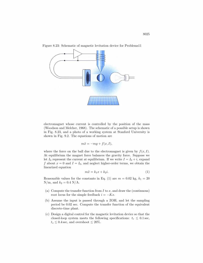
8025
Figure 8.23: Schematic of magnetic levitation device for Problems11
electromagnet whose current is controlled by the position of the mass(Woodson and Melcher, 1968). The schematic of a possible setup is shownin Fig. 8.23, and a photo of a working system at Stanford University isshown in Fig. 9.2. The equations of motion are
m�x = �mg + f(x; I);
where the force on the ball due to the electromagnet is given by f(x; I).At equilibrium the magnet force balances the gravity force. Suppose welet I0 represent the current at equilibrium. If we write I = I0 + i, expandf about x = 0 and I = I0, and neglect higher-order terms, we obtain thelinearized equation
m�x = k1x+ k2i: (1)
Reasonable values for the constants in Eq. (1) are m = 0:02 kg, k1 = 20N=m, and k2 = 0:4 N=A.
(a) Compute the transfer function from I to x, and draw the (continuous)root locus for the simple feedback i = �Kx.
(b) Assume the input is passed through a ZOH, and let the samplingperiod be 0.02 sec. Compute the transfer function of the equivalentdiscrete-time plant.
(c) Design a digital control for the magnetic levitation device so that theclosed-loop system meets the following speci�cations: tr � 0:1 sec,ts � 0:4 sec, and overshoot � 20%.

8026 CHAPTER 8. DIGITAL CONTROL
(d) Plot a root locus with respect to k1 for your design, and discuss thepossibility of using your closed-loop system to balance balls of variousmasses.
(e) Plot the step response of your design to an initial disturbance dis-placement on the ball, and show both x and the control current i.If the sensor can measure x only over a range of �1=4cm and theampli�er can only provide a current of 1 A, what is the maximumdisplacement possible for control, neglecting the nonlinear terms inf(x; I)?
Solution:
(a)
G(s) =X(s)
I(s)=
k2=m
s2 � k1=m(2)
=20
s2 � 1000
(b) T = 0:02 sec,
G(z) = (1� z�1)Z�G(s)
s
�= 0:004135
z + 1
(z � 0:5313)(z � 1:8822)
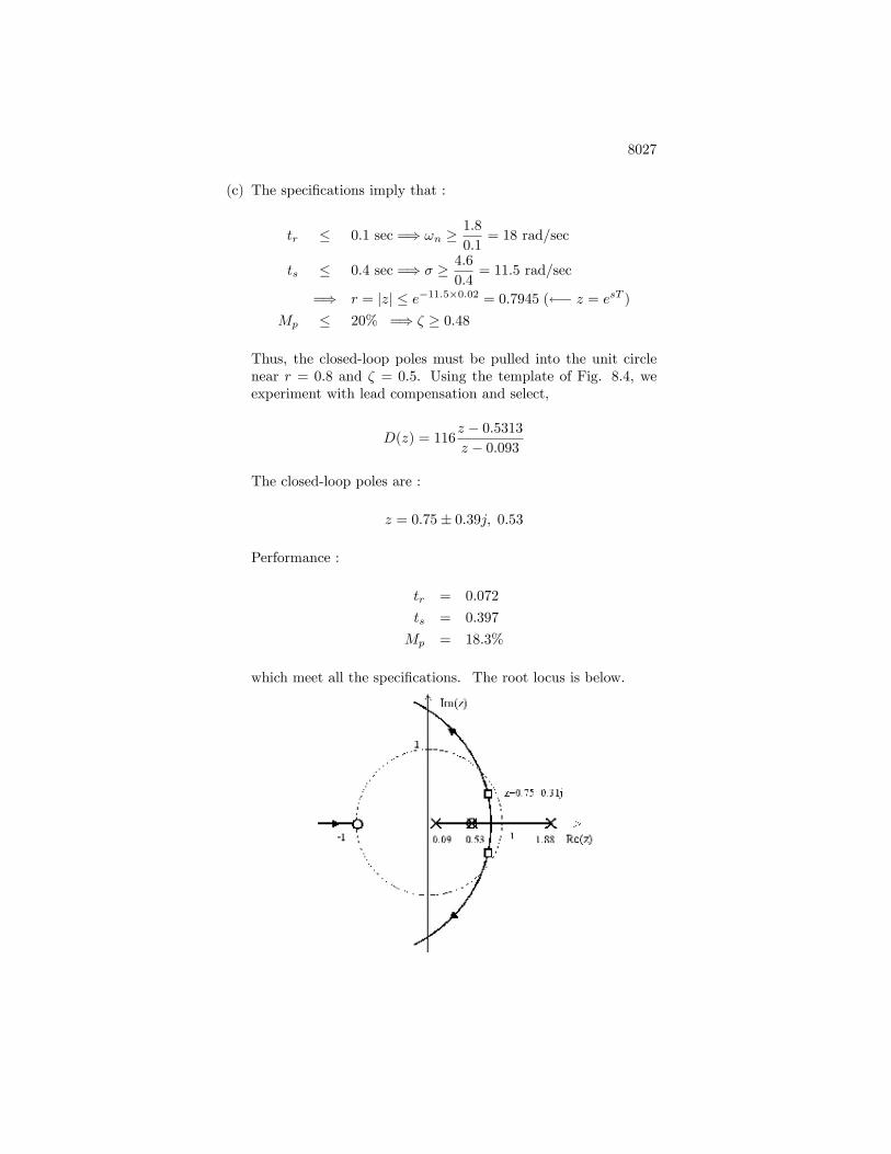
8027
(c) The speci�cations imply that :
tr � 0:1 sec =) !n �1:8
0:1= 18 rad/sec
ts � 0:4 sec =) � � 4:60:4
= 11:5 rad/sec
=) r = jzj � e�11:5�0:02 = 0:7945 ( � z = esT )Mp � 20% =) � � 0:48
Thus, the closed-loop poles must be pulled into the unit circlenear r = 0:8 and � = 0:5. Using the template of Fig. 8.4, weexperiment with lead compensation and select,
D(z) = 116z � 0:5313z � 0:093
The closed-loop poles are :
z = 0:75� 0:39j; 0:53
Performance :
tr = 0:072
ts = 0:397
Mp = 18:3%
which meet all the speci�cations. The root locus is below.

8028 CHAPTER 8. DIGITAL CONTROL
The step response shows Mp
0 0 . 1 0 . 2 0 . 3 0 . 4 0 . 5 0 . 6 0 . 7 0 . 80
1
2
3
4
5
6
7
8C l o s e d L o o p S t e p R e s p o n s e
T i m e ( s e c )
x [m]
0 0 . 1 0 . 2 0 . 3 0 . 4 0 . 5 0 . 6 0 . 7 0 . 8 4 0 0
3 0 0
2 0 0
1 0 0
0
1 0 0
2 0 0T i m e H i s t o r y o f C o n t r o l E f f o r t
T i m e ( s e c )
i [A]
(d) As can be seen from Eq. (2), the loop gain and the open loop polelocations depend on the mass of the ball. Changing the mass

8029
will therefore a¤ect the dynamic characteristics of the systemand may render it unstable. A root locus of the closed-looppoles versus k1 shows how the locus changes as a function of themass:
The closed-loop system becomes unstable for k1 � 24. Since asmall increase in k1 makes the system unstable and a decreasein m has the same e¤ect on the system, it is di¢ cult to balanceballs of smaller masses.
(e) The response to an initial x displacement is shown :
0 0 . 1 0 . 2 0 . 3 0 . 4 0 . 5 0 . 6 0 . 7 0 . 8
1 . 5
1
0 . 5
0
0 . 5
1
C l o s e d L o o p I n i t i a l R e s p o n s e
T i m e ( s e c )
x [m]

8030 CHAPTER 8. DIGITAL CONTROL
0 0 . 1 0 . 2 0 . 3 0 . 4 0 . 5 0 . 6 0 . 7 0 . 8
1 0 0
5 0
0
5 0
1 0 0
T i m e H i s t o r y o f C o n t r o l E f f o r t
T i m e ( s e c )
i [A]
The assumption here is that an allowable transient must stay inthe range of the sensor and not require more than the limit ofthe current. From I(z) = D(z)(0 �X(z)), we have a di¤erenceequation :
i(k)� 0:093i(k � 1) = �116fx(k)� 0:5313x(k � 1)g
For k = 0, i(0) = �116x(0). We see that if x(0) = 1 theni(0) = �116. Note that i(0) = �D(1)x(0).Thus, if i is to be kept below 1A then x(0) must be kept below1=116 = 0:00862 m = 0:862 cm = 0:339 inch, which is greaterthan the sensor range. The current control can handle any dis-placement in the range of �0:25 inch.
12. Repeat Problem 5.27 in Chapter 5 by constructing discrete root lociand performing the designs directly in the z-plane. Assume that theoutput y is sampled, the input u is passed through a ZOH as it entersthe plant, and the sample rate is 15 Hz.
Solution
(a) The most e¤ective discrete design method is to start with some ideawhat the continuous design looks like, then adjust that as necessarywith the discrete model of the plant and compensation. We refer tothe solution for Probelm 5.27 for the starting point. It shows that

8031
the specs can be met with a lead compensation,
D1(s) = K(s+ 1)
(s+ 60)
and a lag compensation,
D2(s) =(s+ 0:4)
(s+ 0:032):
Although it is stated in the solution to Problem 5.27 that a gain,K = 240 will satisfy the constraints, in fact, a gain of about K = 270is actually required to meet the rise time constraint of tr � 0:4 sec.So we will assume here that our reference continuous design is
D1(s) = 270(s+ 1)
(s+ 60)
(s+ 0:4)
(s+ 0:032)
It yields a rise time, tr �= 0:38; Mp�= 15%; andKv = (270)(
160 )(
0:40:32 ) =
56: So all specs are met. For interest, use of the damp function showsthat !n = 6:4 rad/sec for the dominant roots, and those roots havea damping ratio, � �= 0:7: For the discrete case with T = 15 Hz,we should expect some degradation in performance, especially thedamping, because the sample rate is approximately 15�!n:The discrete transfer function for the plant described by G(s) andpreceeded by a ZOH is:
G(z) = (1� z�1)Z�G(s)
s
�=
z � 1zZ�
10
s(s+ 1)(s+ 10)
�This is most easily determined via Matlab,
sysC = tf([10],[1 11 10 0]);T=1/15;sysD = c2d(sysC,T,�zoh�);
which produces:
G(z) = 0:00041424(z + 3:136)(z + 0:2211)
(z � 1)(z � 0:9355)(z � 0:5134The essential elements of the compensation are that the lead providesvelocity feedback with a TD = 1 and the lag provides some highfrequency gain. The discrete equivalent of the proportional pluslead would be (see Eq. 8.42):
D1(z) = K(1 +TDT(1� z�1)) = K (1 + TD=T )z � TD=T
z

8032 CHAPTER 8. DIGITAL CONTROL
which for T = 1=15 = 0:0667 and TD = 1 reduces to
D1(z) = 27016z � 15z�1
z= 4320
z � 0:9375z
:
The lag equivalent is best introduced by use of one of the approxi-mation techniques, such as the matched pole-zero:
D2(z) =z � e�0:4Tz � e�0:032T =
z � :9737z � :9979
as its whole function is to raise the gain at very low frequencies forerror reduction. Examining the resulting discrete root locus andpicking roots with rloc�nd to yield the required damping shows thatthe gain, K = 60:While the use of damp indicates that the frequencyand damping are acceptable, the time response shows an overshootof about 20% and the rise time is slightly below spec. We thereforeneed to increase the lead (move the lead zero closer to z = +1) todecrease the overshoot and increase gain to speed up the rise time.Several iterations on these two quantities indicates that moving thelead zero from z = 0:9375 to z = 0:96 and increasing the gain fromK = 60 to K = 65 meets both specs. The velocity coe¢ cient isfound from and is also satis�ed.
Kv =lim
z ! 1
(z � 1)D(z)G(z)Tz
The time response of the �nal design below shows that all specs aremet.
0 0.2 0.4 0.6 0.8 1 1.2 1.4 1.6 1.8 20
0.2
0.4
0.6
0.8
1
1.2
time (sec)
y
Step Response
13. Design a digital controller for the antenna servo system shown in Figs. 3.61and 3.62 and described in Problem 3.31. The design should provide a step

8033
response with an overshoot of less than 10% and a rise time of less than80 sec.
(a) What should the sample rate be?
(b) Use the matched pole-zero discrete equivalent method.
(c) Use discrete design and the z-plane root locus.
Solution
(a) The equation of motion is :
J�� +B� = Tc
whereJ = 600000 kg.m2; B = 20000 N.m.sec
If we de�ne :
a =B
J=1
30; U =
TcB
after Laplace transform, we obtain :
G(s) =�(s)
u(s)=
1
s(30s+ 1)
From the speci�cations,
Mp < 10% =)MP�=�1� �
0:6
�100 =) � > 0:54
tr < 80 sec =) tr �=1:8
!n< 80 =) !n �= !BW > 0:0225
Note that !pn �= 1=30 < !n.If designing by emulation, a sample rate of 20 times the bandwidthis recommended. If using discrete design, the sample rate can belowered somewhat to perhaps as slow as 10 times the bandwidth.However, to reject random disturbances, best results are obtained bysampling at 20 times the closed-loop bandwidth or faster. Thus, forboth design methods, we choose :
T = 10 sec
!s = 0:628 rad/sec, which is > 20!n = 0:45 rad/sec
(b) Continuous design :Use a proportional controller :
u(s) = D(s)(�r(s)� �(s)) = K(�r(s)� �(s))

8034 CHAPTER 8. DIGITAL CONTROL
Root locus :Choose K = 0:210.The closed-loop pole location in s-plane :
s = �0:0167� 0:0205j
The corresponding natural frequency and damping :
!n = 0:0265; � = 0:6299
Digitized the continuous controller with matched pole-zero method :
D(z) = 0:0210
Tc(z) = Bu(z) = 420(�r(z)� �(z))
Performance :
Mp = 0:119
tr = 67:3 sec
(c) With u(k) applied through a ZOH, the transfer function for an equiv-alent discrete-time system is :
G(z) = Kz + b
(z � 1)(z � eaT )
where
K =aT � 1 + e�aT
a; b =
1� e�aT � aTe�aTaT � 1 + e�aT
=) G(z) = 1:4959z + 0:8949
(z � 1)(z � 0:7165)

8035
Use a proportional control of the form :
D(z) = K
Root locus :
The speci�cation can be achieved with the proportional control. How-ever, we try to achieve the same closed-loop poles as the emulationdesign (part (b)) for comparison. These closed-loop pole locationsare denoted by " + " in the root locus.Use a PD control of the form :
D(z) = Kz � �z
Root locus :

8036 CHAPTER 8. DIGITAL CONTROL
Choose K = 0:0294; � = 0:3.
The resulting z-plane roots :
z = 0:8280� 0:1725j; 0:0165
This corresponds to the s-plane roots :
s = �0:0167�0:0205j (the design point of emulation design); �0:4104
which satisfy the speci�cation :
!n = 0:0265; 0:4104
� = 0:6321; 1:000
The control law :
D(z) = 0:0294z � 0:3z
Tc(z) = Bu(z) = 588z � 0:3z
Performance :
Mp = 0:079
tr = 71:3 sec
Step response :
0 5 0 1 0 0 1 5 0 2 0 0 2 5 0 3 0 00
0 . 2
0 . 4
0 . 6
0 . 8
1
1 . 2S t e p R e s p o n s e
t i m e ( s e c )
x
(m
)
d i s c r e t e d e s i g n
e m u l a t i o n d e s i g n

8037
0 5 0 1 0 0 1 5 0 2 0 0 2 5 0 3 0 0 0 . 0 1
0
0 . 0 1
0 . 0 2
0 . 0 3
0 . 0 4T i m e H i s t o r y o f C o n t r o l E f f o r t
t i m e ( s e c )
u
(T
c/
B)
d i s c r e t e d e s i g n
e m u l a t i o n d e s i g n
14. The system
G(s) =1
(s+ 0:1)(s+ 3)
is to be controlled with a digital controller having a sampling period ofT = 0:1 sec. Using a z-plane root locus, design compensation that willrespond to a step with a rise time tr � 1 sec and an overshoot Mp � 5%.What can be done to reduce the steady-state error?
Solution
(a) Continuous plant :
G(s) =1
(s+ 0:1)(s+ 3); Type 0 system
Discrete model of G(s) preceeded by a ZOH (T = 0:1 sec) :
G(z) = 0:0045z + 0:9019
(z � 0:7408)(z � 0:99)
Speci�cations :
tr � 1 sec �! !n � 1:8 rad/secMp � 5% �! � � 0:7
Discrete design : A simple proportional feedback, D(z) = K = 4:0,will bring the closed-loop poles to :
z = 0:8564� 0:1278j

8038 CHAPTER 8. DIGITAL CONTROL
which are inside the specs region.
!n = 2:07 rad/sec; � = 0:70
Root locus :
Step response :
0 1 2 3 4 5 6 7 80
0 . 1
0 . 2
0 . 3
0 . 4
0 . 5
0 . 6
0 . 7
0 . 8
0 . 9
1C l o s e d L o o p S t e p R e s p o n s e
T i m e ( s e c )
y

8039
0 1 2 3 4 5 6 7 80
1
2
3
4
T i m e H i s t o r y o f C o n t r o l E f f o r t
T i m e ( s e c )
u
The step response shows that :
tr �= 1:02 sec
Mp�= 4:7%
However, since the system is type 0, steady-state error exists and is7% in this case. An integral control of the form,
D(z) =K
TI
Tz
z � 1
can be added to the proportional control to reduce the steady-stateerror, but this typically occurs at the cost of reduced stability.
15. The transfer function for pure derivative control is
D(z) = KTDz � 1Tz
;
where the pole at z = 0 adds some destabilizing phase lag. Can this phaselag be removed by using derivative control of the form
D(z) = KTD(z � 1)T
?
Support your answer with the di¤erence equation that would be required,and discuss the requirements to implement it.
Solution:

8040 CHAPTER 8. DIGITAL CONTROL
(a) No, we cannot use derivative control of the form :
D(z) = KTDz � 1T
to remove the phase lag. The di¤erence equation corresponding to
D(z) = KpTDz � 1T
=U(z)
E(z)
is
u(k) = KpTDe(k + 1)� e(k)
T
This is not a causal system since it needs the future error signalto compute the current control. In real time applications, it is notpossible to implement a non-causal system.

Chapter 9
Nonlinear Systems
Problems and Solutions for Section 9.2: Analysis By Lineariza-tion1. Figure 9.56 shows a simple pendulum system in which a cord is wrapped around a �xed cylinder.The motion of the system that results is described by the di¤erential equation
(l +R�)�� + g sin � +R _�2= 0;
where
l = length of the cord in the vertical (down) position;
R = radius of the cylinder:
(a) Write the state-variable equations for this system.
(b) Linearize the equation around the point � = 0, and show that for small values of � thesystem equation reduces to an equation for a simple pendulum, that is,
�� + (g=l)� = 0:
R u
l
l 1 R u
Figure 9.56: Motion of cord wrapped around a �xed cylinder for Problem 1.
Solution:
9001

9002 CHAPTER 9. NONLINEAR SYSTEMS
(a) This is a second order non-linear di¤erential equation in �. Let x =�_� �
�T.
_x1 = �� = �R_�2+ g sin �
(l +R�)= �Rx
21 + g sinx2(l +Rx2)
;
_x2 = _� = x1:
(b) For small values of �.
(l +R�) �= l;
sin � �= �;
_�2 �= 0:
(a)
l�� + g� = 0
�� +g
l� = 0
2. The circuit shown in Fig. 9.57 has a nonlinear conductance G such that iG = g(vG) = vG(vG �1)(vG � 4). The state di¤erential equations are
di
dt= �i+ v;
dv
dt= �i+ g(u� v);
where i and v are the state variables and u is the input.
(a) One equilibrium state occurs when u = 1 yielding i1 = v1 = 0. Find the other two pairs ofv and i that will produce equilibrium.
(b) Find the linearized model of the system about the equilibrium point u = 1, i = v1 = 0.
(c) Find the linearized models about the other two equilibrium points.
z
i
L 5 1i G
R 5 1u
1
2
C 5 1 v
1
2
2v G1
G
Figure 9.57: Nonlinear circuit for Problem 2.
Solution:(a) Equilibrium:
di
dt= �i+ v = 0;
dv
dt= �i+ g(u� v) = 0;

9003
g(u� v)� i = (u� v) [(u� v)� 1] [(u� v)� 4]� v = 0;
as u = 1,
(1� v)(�v)(�3� v)� v = v�v2 + 2v � 2
�= 0:
v = 0;�1�p3:
So,i = v = 0;�1�
p3:
(b) Let�s replace u, v, and i by 1 + �u, �v, and �i.
�_i = ��i+ �v;� _v = ��i+ g(1 + �u� �v);
= ��i+ (1 + �u� �v)((1 + �u� �v)� 1)((1 + �u� �v)� 4);= ��i+ (1 + �u� �v) (�u� �v) (�u� �v � 3);�= ��i� 3�u+ 3�v:
d
dt
��i�v
�=
��1 1�1 3
� ��i�v
�+
�0�3
��u:
(c) In general the linearized form will be,
d
dt
��i�v
�=
��1 1
�1 @g@v
� ��i�v
�+
�0@g@u
��u;
As u = 1;
g(u; v) = g(1; v) = v�v2 + 2v � 2
�;
@g
@v=
�v2 + 2v � 2
�+ v (2v + 2) ;
= 5� 2p3 when v = �1�
p3:
Also
@g (u� v)@v
= �g0 (u� v) ;
@g (u� v)@u
= g0 (u� v) = �@g@v
= �5� 2p3:
So,d
dt
��i�v
�=
��1 1
�1 5� 2p3
� ��i�v
�+
�0
�5� 2p3
��u:

9004 CHAPTER 9. NONLINEAR SYSTEMS
3. Consider the circuit shown in Fig. 9.58; u1and u2 are voltage and current sources, respectively,and R1 and R2 are nonlinear resistors with the following characteristics:
Resistor 1 : i1 = G(v1) = v31Resistor 2 : v2 = r(i2);
where the function r is de�ned in Fig. 9.59.
(a) Show that the circuit equations can be written as
_x1 = G(u1 � x1) + u2 � x3_x2 = x3_x3 = x1 � x2 � r(x3):
Suppose we have a constant voltage source of 1 Volt at u1 and a constant current sourceof 27 Amps; i.e., uo1 = 1, uo2 = 27. Find the equilibrium state xo = [xo1; x
o2; x
o3]T for the
circuit. For a particular input uo , an equilibrium state of the system is de�ned to be anyconstant state vector whose elements satisfy the relation
_x1 = _x2 = _x3 = 0:
Consequently, any system started in one of its equilibrium states will remain there inde�-nitely until a di¤erent input is applied.
(b) Due to disturbances, the initial state (capacitance, voltages, and inductor current) is slightlydi¤erent from the equilibrium and so are the independent sources; that is,
u(t) = uo + �u(t)x(t0) = xo(t0) + �x(t0):
Do a small-signal analysis of the network about the equilibrium found in (a), displayingthe equations in the form
� _x1 = f11 �x1 + f12 �x2 + f13 �x3 + g1 �u1 + g2 �u2:
(c) Draw the circuit diagram that corresponds to the linearized model. Give the values of theelements.
R 2
x 1
1
2
R 1
v 212
v 121
1 Fzu 1(5 1 V )
1
2
i 1
i 2 5 x 3
1
2
1 Hu 2
(5 2 7 A )
1 F
1 x 2 2
Figure 9.58: A nonlinear circuit for Problem 3.
Solution:

9005
(a)
i1 = G (u1 � x1) ;
i1 � i2 + u2 = Cd
dtx1;
i2 = Cd
dtx2 = x3;
v2 = r (i2) ;
0� x2 + x1 � v2 = Ld
dti2:
C _x1 = G (u1 � x1)� x3 + u2;C _x2 = x3;
L _x3 = x1 � x2 � r (x3) :
As C = L = 1,
_x1 = G (u1 � x1)� x3 + u2;_x2 = x3;
_x3 = x1 � x2 � r (x3) :
(b) Equilibrium state around u01 = 1, u02 = 27.
0 = G�u01 � x01
�� x03 + u02;
= G�1� x01
�� x03 + 27;
0 = x03;
0 = x01 � x02 � r (0) :
i 2
v 2
1
2
2 1 0S l o p e 5 ½
S lo p e 5 1
Figure 9.59: Nonlinear resistance for Problem 3.

9006 CHAPTER 9. NONLINEAR SYSTEMS
G�1� x01
�� x03 + 27 =
�1� x01
�3+ 27 = 0;
x01 = 4;
x02 = x01 � r (0) = 4� 2 = 2;x03 = 0:
x0 =�4 2 0
�T:
� _x1 = G��u01 + �u1
���x01 + �x1
����x03 + �x3
�+�u02 + �u2
�;
= (�3 + �u1 � �x1)3 � �x3 + 27 + �u2;�= �27 + 3� 9 (�u1 � �x1)� �x3 + 27 + �u2;= �27�x1 � �x3 + 27�u1 + �u2:
� _x2 = x03 + �x3;
= �x3:
� _x3 =�x01 + �x1
���x02 + �x2
�� r
�x03 + �x3
�;
= 4 + �x1 � 2� �x2 � (�x3 + 2) ;= �x1 � �x2 � �x3:
(c) Circuit diagram:
Linear circuit model for Problem 9.3.
L = 1H; R1 =127; R2 = 1:
4. Consider the nonlinear system
_x = �x2e� 1x + sinu x(0) = 1
a) Assume uo = 0 and solve for xo(t).
b) Find the linearized model about the nominal solution in part (a).
Solution:

9007
(a)
_x(t) = �x2e� 1x ;
dx
dt= �x2e� 1
x ;
�x�2e 1x dx = dt:
Integrate both sides:
Z x(t)
x(0)
� 1x2e1x dx =
Z t
0
dt;
e1
x(t) � e 11 = t;
xo(t) =1
log(t+ e):
(b)
_x = �x2e� 1x + sinu;
� _x = �h2xe�
1x + e�
1x
i�x+ cosu �u.
For the equilibrium conditions of part (a),
� _x = � 1
t+ e
�1 +
2
log(t+ e)
��x+ �u.
5. Linearizing e¤ect of feedback. We have seen that feedback can reduce the sensitivity of theinput-output transfer function with respect to changes in the plant transfer function , andreduce the e¤ects of a disturbance acting on the plant. In this problem we explore anotherbene�cial property of feedback: it can make the input-output response more linear than theopen-loop response of the plant alone. For simplicity let us ignore all the dynamics of the plant,and assume that the plant is described by the static nonlinearity
y(t) =
�u u � 1u+12 u > 1
a) Suppose we use proportional feedback
u(t) = r(t) + �(r(t)� y(t))
where � � 0 is the feedback gain. Find an expression for y(t) as a function of r(t) for theclosed-loop system (This function is called the nonlinear characteristic of the system.) Sketchthe nonlinear transfer characteristic for � = 0 (which is really open-loop), � = 1, and � = 2.
b) Suppose we use integral control,
u(t) = r(t) +
Z t
0
(r(�)� y(�))d�

9008 CHAPTER 9. NONLINEAR SYSTEMS
The closed-loop system is therefore nonlinear and dynamic. Show that if r(t) is a constant, sayr, then lim
t!1y(t) = r. Thus, the integral control makes the steady-state transfer characteristic
of the closed-loop system exactly linear. Can the closed-loop system be described by a transferfunction from r to y?
Solution:
(a)
Fig 10
6:pdf
Problem 9.5. Nonlinear system with saturation: proportional control.
For u � 1:
y = r + �(r � y) = (1 + �)y = (1 + �)r; y = r = u:
For u > 1:
y =u+ 1
2=1
2+1
2[r + �(r � y)];
2y = 1 + r + �r � �y;(2 + �)y = 1 + (1 + �)r;
y =1 + (1 + �)r
2 + �: See Figure on top of the next page.
if � = 0 then y =1 + r
2:
if � = 1 then y =1
3+2
3r:
if � = 2 then y =1
4+3
4r: See middle Figure on the next page.

9009
0 0.5 1 1.5 2 2.5 3 3.5 40
0.5
1
1.5
2
2.5
3Openloop vs closedloop
r
y
OL
CL
0 0.5 1 1.5 2 2.5 3 3.5 40
0.5
1
1.5
2
2.5
3Openloop vs closedloop
r
y
OL
CL
Problem 9.5. Open-loop vs closed-loop response.

9010 CHAPTER 9. NONLINEAR SYSTEMS
0 0.5 1 1.5 2 2.5 3 3.5 40
0.5
1
1.5
2
2.5
3
3.5Openloop vs closedloop for various α
r
y
OL
α=1
α=2
0 0.5 1 1.5 2 2.5 3 3.5 40
0.5
1
1.5
2
2.5
3
3.5Openloop vs closedloop for various α
r
y
OL
α=1
α=2
Problem 9.5. Open-loop vs closed-loop response for various values of �:
(b)
Fig 11
9:pdf
Problem 9.5. Nonlinear system with saturation: integral control.
u = r +
Z t
0
(r � y)dt;
r = cons tan t;

9011
u < 1,
y = r +
Z t
0
(r � y)dt;
Y = R+R� Ys
;
(1 + s)Y = (1 + s)R; Y = R
Assume stable: y stays bounded,
y ! y1;
y = r +
Z t
0
(r � y1)dt!1 if y1 6= r;
) y1 = r;
_y = r � y;_y + y = r:
u > 1,
y =1
2+1
2(r +
tZ0
(r � y)dt;
y = f(u);
_x = r � y;
_y =1
2(r � y);
2 _y + y = r;
Y (s)
R(s)=
1
2s+ 1:
In the steady-state: y = r:
6. This problem shows that linearization does not always work. Consider the system
_x = �x3 x(0) 6= 0
a) Find the equilibrium point and solve for x(t).
b) Assume � = 1. Is the linearized model a valid representation of the system?
c) Assume � = �1. Is the linearized model a valid representation of the system?Solution: (a) The equilibrium point is found from:
_x = �x3 = 0;
) xe = 0:

9012 CHAPTER 9. NONLINEAR SYSTEMS
To determine x(t) we re-write the system equation as,
dx
x3= �dt;
Integrating both sides:
Z x(t)
x(0)
dx
x3= �
Z t
0
dt;
�12x�2jx(t)x(0) = �t;
x2 =x(0)2
1� 2�x(0)2t ;
x(t) =1p
x(0)�2 � 2�t: (�)
(b) If � = 1 the linearized system is,
� _x = 3(1)x2e = 0;
�x = cons tan t,
that is the linear system is not asymptotically stable (it is neutrally stable). However, we cansee from the nonlinear solution given by Equation (*) that the system is unstable and exhibits a�nite �escape-time�at t = 1
2x(0)�2 (i.e., the response of the nonlinear system tends to in�nity in
�nite time;see Figure on the next page). The linear system does not predict qualitative behaviorof the nonlinear system. So the linear model is not a valid representation of the system.
(c) If � = �1 the linearized system is
� _x = 3(�1)x2e = 0;�x = cons tan t,
that is the linear system is not asymptotically stable (it is neutrally stable). However, we cansee from the nonlinear solution given by Equation (*) that the system is asymptotically stableas x2 starts o¤ at x2o but drops o¤ to zero (see Figure on top of the next page). The linearsystem does not predict qualitative behavior of the nonlinear system. So the linear model is nota valid representation of the system. The two systems corresponding to � = +1 and � = �1have the same linearized system but very di¤erent nonlinear behavior. The conclusion is thatthe linearized system usually gives a good idea of the system behavior around the equilibrium(xe) but not always.

9013
0 20 40 60 80 1000
0.5
1
1.5
2
2.5
Time (sec)
x(t)
0 20 40 60 80 1000
0.5
1
1.5
2
2.5
Time (sec)
x(t)
Problem 9.6: Behavior of nonlinear system.
7. Consider the object moving in a straight line with constant velocity shown in Figure 9.60. Theonly available measurement is the range to the object. The system equations are
24 _x_v_z
35 =24 0 1 00 0 00 0 0
3524 xvz
35
where
z = cons tan t
_x = cons tan t = v0
r =px2 + z2
Derive a linear model for this system.

9014 CHAPTER 9. NONLINEAR SYSTEMS
Solution: This system has only an output nonlinearity,
y = r = h(x);
�r =�h
@x�x = H�x;
H =�
�h@x
�h@v
�h@z
�;
=�xr 0 z
r
�:
_x = Fx;
�r =�xr 0 z
r
�x:
Problems and Solutions for Section 9.3: Equivalent GainAnalysis Using Root Locus
8. Consider the third-order system shown in Fig. 9.61.
(a) Sketch the root locus for this system with respect to K, showing your calculations for theasymptote angles, departure angles, and so on.
(b) Using graphical techniques, locate carefully the point at which the locus crosses the imag-inary axis. What is the value of K at that point?
(c) Assume that, due to some unknown mechanism, the ampli�er output is given by the fol-lowing saturation non linearity (instead of by a proportional gain K):
u =
8<: e; jej � 1;1; e > 1;�1; e < �1:
Qualitatively describe how you would expect the system to respond to a unit step input.Solution:
(a) The locus branches leave the origin at angles of 180�and �60�. Two break in at angles of�90� near s = �3. See root locus plot.(b) The locus crosses the imaginary axis at ! = 1 for K = 0:5.
(c) The system is conditionally stable and with saturation would be expected to be stable forsmall inputs and go unstable for large inputs.
O b j e c t
z
x0
Figure 9.60: Diagram of moving object for Problem 9.7.

9015
6 5 4 3 2 1 0 1
2.5
2
1.5
1
0.5
0
0.5
1
1.5
2
2.5
Root Locus
Real Axis
Imag
inar
y Ax
is
Root locus for Problem 9.8.
(a) Problems and Solutions for Section 9.4: Equivalent GainAnalysis Using Frequency Response: Describing Func-tions
9. Compute the describing function for the relay with deadzone nonlinearity shown in Figure 9.6(c).
YS
2
1
KRs 3
( s 1 1 ) 2e u
Figure 9.61: Control system for Problem 9.8.

9016 CHAPTER 9. NONLINEAR SYSTEMS
Solution:
Y1 =1
�
Z 2�
0
y(t) sin(!t)d(!t)
=4
�
Z �2
0
y(t) sin(!t)d(!t)
=4N
�
Z �2
!t1
sin(!t)d(!t)
=4N
�cos(!t1):
Since !t1 =ha then cos(!t1) =
q1�
�ha
�2:
The describing function is then given by,
DF =Y1a=4N
�a
s1�
�h
a
�2:
10. Compute the describing function for gain with dead zone nonlinearity shown in Figure 9.6 (d).
Solution: This is an odd nonlinearity so that all the cosine terms are zeros and the DF is real:
Y1 =1
�
Z 2�
0
y(t) sin(!t)d(!t);
=4
�
Z �2
0
y(t) sin(!t)d(!t);
=4Ko
�
Z �2
0
(A sin(!t)� a) sin(!t)d(!t):
Since h = a sin(!t1) then !t1 = sin�1 � h
�
�;
Y1 =4aKo
�
"Z �2
!t1
(sin2(!t)� sin(!t1) sin(!t))d(!t)#;
=2aKo
�
"�
2� sin�1
� aA
�� a
A
r1�
� aA
�2#:
The describing function is then given by,
DF =Y1a=2Ko
�
24�2� sin�1
�h
a
�� h
a
s1�
�h
a
�235 :11. Compute the describing function for the preloaded spring or Coulomb plus viscous friction
nonlinearity shown in Figure 9.6 (e).
Solution: This is a combination of a gain, K0, plus a relay nonlinearity (see Example 9.11).Therefore,
DF =K0a
a+4N
�a= K0 +
4N
�a:

9017
12. Consider the quantizer function shown in Figure 9.62 that resembles a staircase. Find thedescribing function for this nonlinearity and write a Matlab .m function to generate it.
d 1 d 2 d 3 d 4
hu
q
2 q
3 q
4 q
y
Figure 9.62: Quantizer nonlinearity for Problem 12.
Solution. The abscissa breakpoints are denoted by �i. From Eq. 9.23,
b1 =4
�
Z �2
0
f (a sin!t) sin!t d(!t)
=4
�
Z '1
0
0 � sin!t d(!t) +Z '2
0
q � sin!t d(!t) + :::+Z 'n
0
nq � sin!t d(!t)
=4
�(cos'1 + cos'2 + :::+ cos'n);
where,
i = sin
��ia
�i = 1; :::; n:
The describing function is then given by,
Keq(a) =b1a=
8><>:0 0 < a < q
2
4q�a
nXi=1
q1�
�2i�12a q
�2 2n�12 q < a < 2n+1
2 q
The following shows the Matlab .m function:
% Feedback Control of Dynamic Systems, 6e
% Franklin, Powell, Emami
% Problem 9.12

9018 CHAPTER 9. NONLINEAR SYSTEMS
clear all;
close all;
na = 99;
nn = 6;
Keq=zeros(1,nn*na);
for n=1:nn
ai = linspace((2*n-1)/2, (2*n+1)/2, na);
for ni=1:na
for k=1:n
Keq((n-1)*na+ni) = Keq((n-1)*na+ni) + (4/(pi*ai(ni)))*sqrt(1- ((2*k-1)/(2*ai(ni)))^2);
end;
end;
end;
plot(linspace(1/2,(2*nn+1)/2,na*nn),Keq);
title(�Describing function for quantizer nonlinearity�)
xlabel(�a/q�)
ylabel(�K_{eq}�)
grid;
hold o¤
The describing function is plotted in the �gure as a function of aq . The maximum of the DFoccurs at Keq =
4� = 1:27 corresponding to
aq = 0:7. Since the staircase can be approximated
by a straight line, it is seen that the DF will in the limit approach the slope of the linearapproximation, that is one.

9019
0 1 2 3 4 5 6 70
0.2
0.4
0.6
0.8
1
1.2
1.4Describing function for quantizer nonlinearity
a/q
Keq
0 1 2 3 4 5 6 70
0.2
0.4
0.6
0.8
1
1.2
1.4Describing function for quantizer nonlinearity
a/q
Keq
13. Derive the describing function for the ideal contactor controller shown in Figure 9.63. Is itfrequency dependent? Would it be frequency dependent if it had a time delay or hysteresis?Graphically, sketch the time histories of the output for several amplitudes of the input anddetermine the describing function values for those inputs.
O u t p u t
I n p u td
T
Figure 9.63: Contactor for Problem 9.13.

9020 CHAPTER 9. NONLINEAR SYSTEMS
Solution:
Y1 =1
�
Z 2�
0
y(t) sin(!t)d(!t)
=4
�
Z �2
0
y(t) sin(!t)d(!t)
=4T
�
Z �2
!t1
sin(!t)d(!t)
=4T
�cos(!t1):
Si nce !t1 =d
athen cos(!t1) =
s1�
�d
a
�2:
The describing function is then given by,
DF =
(Y1a =
4T�a
q1�
�da
�2d < a
0 a < d
and is not frequency dependent. See Figure on top of the next page. Frequency dependencewill be introduced with a delay.

9021
0 1 2 3 4 50
1
2
3
4
5
6
7
a
Keq
Describing function: DF
0 1 2 3 4 50
1
2
3
4
5
6
7
a
Keq
Describing function: DF
Problem 9.13. DF for d = 0:1, T = 1:0.
0 10 20 30 40 50 60 70 80 900
0.5
1
1.5
2
2.5
3
ω t0
a/d

9022 CHAPTER 9. NONLINEAR SYSTEMS
Problem 9.13. DF values for several di¤erent input frequencies.
14. A contactor controller of an inertial platform is shown in Figure 9.64 where
I = 0:1kgm2
I
B= 10 sec
h
c= 1
J
c= 0:01 sec
�L = 0:1 sec
�f = 0:01 sec
d = 10�5rad
T = 1Nm
The required stabilization resolution is approximately 10�6 rad
K'm> d for '
m> 10�6rad
Discuss the existence, amplitude and frequency of possible limit cycles as a function of the gainK and the DF of the controller. Repeat the problem for a deadband with hysteresis.
I s 1 B1
s1
dT
M o t o r a n d c o n t r o l l e rG i m b a l l e d
G y r o
wv
w mKt L s 1 1t f s 1 1
hc s ( s 1 1 )J
c
Figure 9.64: Block diagram of the system for Problem 9.14.
Solution: Limit cycles depend on the natural behavior of the closed-loop part. The DF of theswitch = Keq: Characteristic equation is:
KG+ 1 = 0
K
B
h
c=
Keq
s��Jc
�s+ 1
� ��Ls+ 1�fs+ 1
�1��
IB
�s+ 1
� + 1 = 0:�KeqK
0:01
��0:1s+ 1
s(10s+ 1)(0:01s+ 1)2
�= �1:
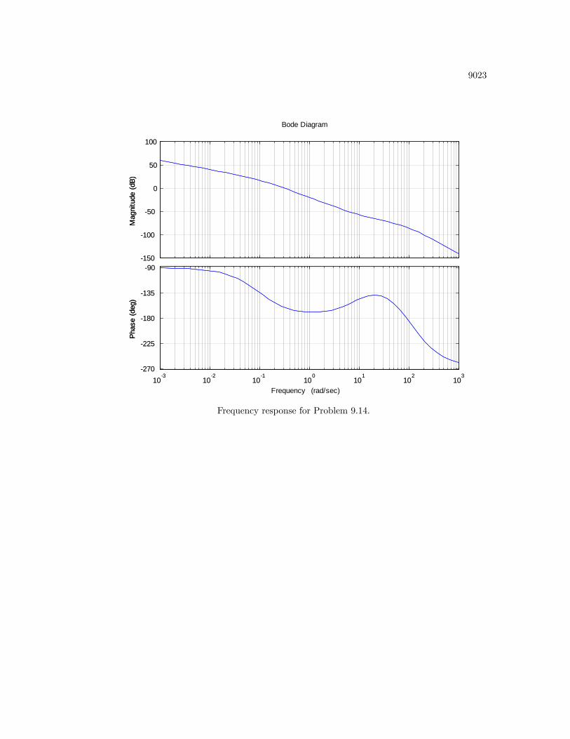
9023
150
100
50
0
50
100M
agni
tude
(dB)
103
102
101
100
101
102
103
270
225
180
135
90
Phas
e (d
eg)
Bode Diagram
Frequency (rad/sec)
150
100
50
0
50
100M
agni
tude
(dB)
103
102
101
100
101
102
103
270
225
180
135
90
Phas
e (d
eg)
Frequency response for Problem 9.14.

9024 CHAPTER 9. NONLINEAR SYSTEMS
150 100 50 0 50
100
50
0
50
100
Root Locus
Real Axis
Imag
inar
y Ax
is
Root locus for Problem 9.14.
Condition for limit cycle is \ = �180� which occurs at � 95 rad/sec and magnitude = 1 (seeFigure) but
KKeq
0:01� 1
10� 10�5 (the value at ! ' 95 rad= sec);
KKeq = 100(rad= sec)(nm sec =rad) = 100 nm;
Keq =4T
�d
�d
a
�s1�
�d
a
�2:
with maximum at 4T�d . But note from the �gure below,
Fig

9025
8
22:pdf
Response for nonlinear system for Problem 9.14.
that for levels of say a > 3d, the output is a constant. The frequency of the limit cycle is �xedby the phase! So ' is constant. The result is independent of K, for large enough K to insurethat K'� d. This is consistent with KKeq = cons tan t for Keq =
cons tan ta , a = K',
KeqK =
�cons tan tK'
�K =
cons tan t'
= cons tan t for K' >> d.
The amplitude is:
Fig 9
23:pdf
Time histories for Problem 9.14.

9026 CHAPTER 9. NONLINEAR SYSTEMS
See above �gures:
1
2
T
I�t2 = ' = 5
rad
sec2(�t)2;
�t =P
4; ! =
2�
P�= 100
rad
sec;
�t =2�
4!=3:14
200= 1:57� 10�2 sec;
' = 12� 10�4 rad:
If the resolution of platform picko¤ should be � 10�6rad and �short� term sensor noise �10�6rad, then K'm >> d is satis�ed, say,
K � 10�6 = d = 10�5 rad;
) K = 10:
KKeq = 100 nm;
) Keq = 10 nm:
Keq =4T
�d
�d
a
�s1�
�d
a
�2� 4� 1� � 10�5
�d
a
�= 10:
d
a= 0:8� 10�5 � 10 = 8� 10�5:
To check:
a =d
8� 10�5 = 0:125� 105 � 10�5 = 0:125 rad:
Here we must consider the mid frequency model because the limit cycle is at ! = 100 rad/sec.! gets integrated in the gyro below its break frequency but 'm goes through the lead circuit fora gain of 10 and K = 10 so a = 12:5� 10�4rad�100 = 0:125 rad as before, so it checks.
15. Nonlinear Clegg Integrator There have been some attempts over the years to improve upon thelinear integrator. A linear integrator has the disadvantage of having a phase lag of 90� at allfrequencies. In 1958, J. C. Clegg suggested that we modify the linear integrator to reset itsstate, x, to zero whenever the input to the integrator, e, crosses zero (i.e., changes sign). TheClegg integrator has the property that it acts like a linear integrator whenever its input andoutput have the same sign. Otherwise, it resets it output to zero. The Clegg integrator canbe described by
x(t) = e(t) if e(t) 6= 0;x(t+) = 0 if e(t) = 0;
where the latter equation implies that the state of the integrator, x, is reset to zero immediatelyafter e changes sign. The Clegg integrator can be implemented with op-amps and diodes. Apotential disadvantage of the Clegg integrator is that it may induce oscillations. (a) Sketch theoutput of the Clegg integrator if the input is e = a sin(!t). (b) Prove that the DF for the Cleggintegrator is
N(a; !) =4
�!� j 1
!:
and this amounts to a phase lag of only 38�. Solution: (a) See Figure below.

9027
0 1 2 3 4 5 6 72
1.5
1
0.5
0
0.5
1
1.5
2Input: a sin(ω t), Output: a/ω (1cos(ω t))
ω t
inpu
t, ou
tput
inputoutput
Plots of the input and output signals.
(b)
a1 =2
�
Z �
0
x(t) cos(!t)d(!t)
=2
�
Z �
0
a
!cos(!t)d(!t)
=2a
�!
Z �
0
cos(!t)d(!t)�Z �
0
cos2(!t)d(!t)
=2a
�!
�0 +
�
2
�= � a
!:
b1 =2
�
Z �
0
x(t) sin(!t)d(!t)
=2
�
Z �
0
a
!(1� cos(!t)) sin(!t)d(!t)
=2a
�!
Z �
0
sin(!t)d(!t)�Z �
0
cos(!t) sin(!t)d(!t)
=2a
�!(2 + 0) =
4a
�!:

9028 CHAPTER 9. NONLINEAR SYSTEMS
The describing function is then given by,
DF =Y1a=
4
�!� j 1
!
=1
!
s1 +
�4
�
�2arctan
���4
�=
1:619
�\� 38:15�:
�Problems and Solutions for Section 9.5: Analysis and De-sign Based on Stability
16. Compute and sketch the optimal reversal curve and optimal control for the minimal time controlof the plant
_x1 = x2
_x2 = �x2 + ujuj � 1
Use the reverse time method and eliminate the time.
Solution: Use the reverse time method and eliminate the time:
_x1 = �x2;_x2 = x2 � u:
For u = +1;time reversal means that we let � = �t, and that changes the sign on the systemand the input matrices,
dx
d�= �Fx�Gu:
In our case,
_x1 = �x2;_x2 = x2 � 1;
dx2d�
= x2 � 1;
dx2(x2 � 1)
= d� :
Integrate both sides: Z x2
0
dx2(x2 � 1)
=
Z �
0
d� :
ln(x2 � 1) = � + C1:

9029
Since x2(0) = 0 then,
C1 = ln(�1);ln(x2 � 1)� ln(�1) = � ;
ln(1� x2) = � ;
x2 = 1� e� ;� = ln(1� x2):
Now,
_x1 = �x2;_x1 = �1 + e� ;
dx1 = (�1 + e� )d� :
Integrate both sides: Z x1
0
dx1 =
Z �
0
(�1 + e� )d�:
x1 = e� � � � 1:
Eliminate � to get,x1 = �x2 � ln(1� x2):
This is the reversal curve for u = 1, x2 < 0.
For u = �1,
_x2 = x2 + 1;
dx2x2 + 1
= d� :
Integrate both sides: Z x2
0
dx2x2 + 1
=
Z �
0
d� :
ln(x2 + 1) = � + C1:
Since x2(0) = 0 then
ln(x2 + 1) = � + C1;
) C1 = ln(1);
ln(x2 + 1) = � ;
x2 + 1 = e� ;
x2 = e� � 1;) � = ln(x2 + 1):

9030 CHAPTER 9. NONLINEAR SYSTEMS
Now,
_x1 = �x2 = 1� e� ;dx1 = (1� e� )d� :
Integrate both sides: Z x1
0
dx1 =
Z �
0
(1� e� )d� ;
x1 = �e� + � + C2;x2(0) = 0; C2 = 1;
x1 = �e� + � + 1:
Eliminate � to get,x1 = ln(1 + jx2j)� x2:
This is the reversal curve for u = �1, x2 > 0.We can then write in general, for all x2,
x1 = sgn(x2) ln(1 + jx2j)� x2
Therefore, the control law is:
u = �sgn[x1 + x2 � sgn(x2) ln(1 + jx2j)]:
Fig 14
25:pdf
Optimal reversal curve for Problem 9.15.

9031
17. Sketch the optimal reversal curve for the minimal time control with juj � 1 of the linear plant
_x1 = x2
_x2 = �2x1 � 3x2 + u:
Solution: We reverse time that means � = �t, and that changes the sign on the system andthe input matrices,
dx
d�= �Fx�Gu:
In our case,
_x1 = �x2_x2 = +2x1 + 3x2 � u:
We simulate the system using the Matlab lsim function with u = +1 and store x1 and x2, andrepeat with u = �1 and store x1 and x2 and plot the results to obtain the optimal reversal curveshown in the plot on the next page:
%Franklin, Powell, Emami 6e
%Problem 9.17
t=0:.01:1;
F=[0 1;-2 -3];
G=[0;1];
H=[1 0];
J=[0];
% Using the reverse time method
sys=ss(-F,-G,H,J);
%u=+1;
[yp,t,xp]=lsim(sys,ones(101,1),t);
plot(xp(:,1),xp(:,2));
hold on;
%u=-1
[ym,t,xm]=lsim(sys,-1*ones(101,1),t);
plot(xm(:,1),xm(:,2));
grid;
xlabel(�x_1�);
ylabel(�x_2�);
title(�Optimal reversal curve�);

9032 CHAPTER 9. NONLINEAR SYSTEMS
1.5 1 0.5 0 0.5 1 1.55
4
3
2
1
0
1
2
3
4
5
x1
x 2
Optimal reversal curve
1.5 1 0.5 0 0.5 1 1.55
4
3
2
1
0
1
2
3
4
5
x1
x 2
Optimal reversal curve
Optimal reversal curve for Problem 9.16.
18. Sketch the time optimal control law for
_x1 = x2
_x2 = �x1 + ujuj � 1
and show a trajectory for x1(0) = 3, and x2(0) = 0.
Solution: u = +1,
sX1(s) = �X2(s);
sX2(s) = X1(s)�1
s;
X2(s) = � 1
s2 + 1;
x2(t) = � sin(t);_x2 = � cos(t) = x1 � 1;x1 = +1� cos(t):

9033
We see that,(x1 � 1)2 + x22 = 1
that is a circle with center at (1; 0); x2 < 0:
Similarly for u = �1 we get,
x2(t) = sin(t)
x1(t) = cos(t)� 1(x1 + 1)
2 + x22 = 1;
that is a circle with center at (�1; 0); x2 > 0:
Fig 12
27:pdf
Reversal curves for Problem 9.18.
The trajectories for this system are circles centered at (�1; 0). This is called the Bushawproblem in optimal control literature.
19. Consider the thermal control system shown in Figure 9.65. The physical plant can be a room,an oven, etc.
(a) What is the limit cycle period?
(b) If Tr is commanded as a slowly increasing function, sketch the output of the system, T .Show the solution for Tr �large�.Solution:(a) This is a �rst order system so use (T; t) plot. For an oven, it is piecewise linear
_T + aT = BN sgn(e) with hysteresis
with
Tr = 800�C;
BN
a� 1000�C above T = 0 (say room temperature)

9034 CHAPTER 9. NONLINEAR SYSTEMS
S
1
2
yTT
N
h
e Bs 1 a
1
S e n s o r
Figure 9.65: Thermal system for Problem 9.19.
a ' 0:01 sec�1; plot vs at; h � 100�C; To = 0:
(b)
limit cycle period , P = ton + toff ;
Tre�at = (Tr � h)
gives toff , �BN
a� (Tr � h)
�e�at =
�BN
a� Tr
�gives ton,
aP = � ln�700
800
�� ln
�200
300
�,
P = 100(0:058 + 0:176) = 23:4 sec :
0 1 2 3 4 5 6
x 104
0
100
200
300
400
500
600
700
800
900
Time (sec)
T (C
)
Temperature output for Problem 9.19.
(c) See Figure below.

9035
0 1 2 3 4 5 6
x 104
0
100
200
300
400
500
600
700
800
900
1000
T (C
)
T ime (sec
Temperature output for reference input Tr = 3t for Problem 9.19.
20. Several systems such as spacecraft, spring-mass system with resonant frequency well below thefrequency of switching, a large motor driven load with very small friction, etc. can be modeledas just an inertia. For an ideal switching curve, sketch the phase portraits of the system. Theswitching function is e = � + �!. Assume � = 10 sec, and the control signal = 10�3 rad/sec2.Now sketch the results with,
a) deadband,
b) deadband plus hysteresis,
c) deadband plus time delay T ,
d) deadband plus a constant disturbance.
Solution:
(a)
d!
d�=
u
!=10�3rad= sec2
!;
!2
2= u �;
� = 500 !2;
! = 10�2 ! � = 0:05:

9036 CHAPTER 9. NONLINEAR SYSTEMS
Fig 1
31:pdf
Phase portraits for deadband for Problem 9.20.
(a)
Fig 2
32:pdf
Phase portraits for deadband for Problem 9.20.
(b)

9037
Fig 3
33:pdf
Phase portraits for deadband plus hysteresis for Problem 9.20.
(c)
Fig 4
34:pdf
Phase portraits for deadband plus plus time delay T for Problem 9.20.

9038 CHAPTER 9. NONLINEAR SYSTEMS
(d)
T! = ��;
�� + �! = 0;
changes slope to �� = ��! + T! = �(� � T )!;_� = ! u! 0 at t for (� � d+ h+ �! = 0) + T;_! = u+D ts ! �s = ��!s + (d� h);! = (u+D)t+ !o;
) � = (u+D)t2
2+ !st+ �s;
for t = T; � = !s(T � �)| {z }new slope
+ (d� h) +�u+D
2
�T 2| {z }
new intercept
:
Reference:[1] D. Graham and D. McRuer, Analysis of Nonlinear Control Systems, John Wiley & Sons,1961.
21. Compute the amplitude of the limit cycle in the case of satellite attitude control with delay
I �� = N u(t��)
usingu = �sgn(� _� + �)
Sketch the phase plane trajectory of the limit cycle and time history of � giving the maximumvalue of �.
Solution: Since the delay is � seconds, _� must travel �NI units during the delay. We canobtain the following relations:
_� =N
I(t� t0) + _�0;
� =1
2
N
I(t� t0)2 + _�0(t� t0) + �0:
Eliminating (t� t0), we get
� � �0 =I
2N( _�2 � _�20) =
I
2N( _�2 � 0);
� =2N
I(� � �0) +
I
2N_�2);
and
� + � _� = 0;
� =1
a:

9039
Fig 6
35:pdf
Phase-plane trajectory of limit cycle for Problem 9.21.
From the geometry of the limit cycle (see above Figure),
_�A +�N
I= _�B ; (2)
At point A,
�A � �0 =I
2N_�2
A; (3)
�A + � _�A = 0; (4)
At point B,
_�2
B
�I
2N
�= ��0; (5)
We need to solve the above four equations for �0 (for �max = �0, �0 = 0).
It seems to be easiest to �rst eliminate �0 using Eqs. (3) and (5) to get
�A +I
2N
h_�2
B � _�2
A
i= 0:
If we eliminate _�B using Eq. (2), then,
�A = ��
2
�2_�A +
�N
I
�= 0:
If we use Eq. (4) to eliminate �A,
� _�A =�
2
�2_�A +
�N
I
�= 0:

9040 CHAPTER 9. NONLINEAR SYSTEMS
Solve for _�A,
_�A =�2N
2I
�1
� ��
�:
From Eq. (2),
_�B +N�
I=�2N
2I
�1
� ��
�:
Then using Eq. (5),
��0 =I
2N
��2N
2I
�1
� ��
�+�N
I
�2;
or,
j�0j =I
2N
��N(� + 2(� ��))
2I(� ��)
�2;
j�0j =N�2
8I
�2� ��� ��
�2= j�maxj:
Time history shown in the Figure below and shows a �nonlinear oscillator.�
Fig 7
36:pdf
Nonlinear oscillator for Problem 9.21.
22. Consider the point mass pendulum with zero friction as shown in Figure 9.66. Using the methodof isoclines as a guide, sketch the phase-plane portrait of the motion. Pay particular attentionto the vicinity of � = �. Indicate a trajectory corresponding to spinning of the bob around andaround rather than oscillating back and forth.
(a) Solution: The equations are:
I�� = mgl sin �;
ml2�� = mgl sin �;
�� =g
lsin �;

9041
lu
M
Figure 9.66: Pendulum for Problem 9.21.
For � � 0, sin � � �;
�� =g
l�;
s2 =g
l;
s = �rg
l:
There is a �saddle�point at � = 0; 2�; :::.
For � � �, sin � � ��;
�� = �gl�;
s2 = �gl;
s = �jrg
l:
There is a �center�at � = ��;�3�; :::.
Using isoclines:
�� = _�d _�
d�=g
lsin �
� =d _�
d�=g
lsin �:
The isoclines are sinusoidal curves. The phase portraits are shown in the Figure below.The upper and lower portraits correspond to the �whirling motion�with pendulum goinground and round.

9042 CHAPTER 9. NONLINEAR SYSTEMS
x ' = yy ' = sin(x)
8 6 4 2 0 2 4 6 8
3
2
1
0
1
2
3
x
y
Phase portraits for Problem 9.22.
NOTE:The phase portraits can be generated using the ODE Software in Matlabpplane7.m (for Matlab Version 7) by Professor John C. Polking at Rice Univer-sity available on the Web at:
http://math.rice.edu/~d�eld/
23. Draw the phase trajectory for a system
�x = 10�6 m/ sec2
between _x(0) = 0, x(0) = 0 and x(t) = 1mm. Find the transition time, tf , by graphical meansfrom the parabolic curve by comparing your solution with several di¤erent interval sizes and theexact solution.
Solution: The phase portrait is shown in the �gure below.

9043
0 0.2 0.4 0.6 0.8 10
0.005
0.01
0.015
0.02
0.025
0.03
0.035
0.04
0.045
x [mm]
v [m
m/s
ec2 ]
Phase portrait
0 0.2 0.4 0.6 0.8 10
0.005
0.01
0.015
0.02
0.025
0.03
0.035
0.04
0.045
x [mm]
v [m
m/s
ec2 ]
Phase portrait
Phase portrait for Problem 9.23.
�x = a;_v
_x=a
v;
v2
2= ax and a = 10�6;
v =p2ax = at+ vo = at;
x(t) =a
2t2 + vot+ xo = 5� 10�7t2 = 1� 10�3;
t2 =
�1
5
�� 104 ) tf = 45 sec :
v =�x
�t:
To obtain t graphically, i.e., by graphical integration, we write,
�t =�x
v;
where v is the �average�v in a given interval of �x. In the �gure above, we divide x into �ve

9044 CHAPTER 9. NONLINEAR SYSTEMS
intervals and �nd (going from left to the right),
tf = �t1 +�t2 +�t3 +�t4 +�t5
=0:2
0:01+
0:2
0:025+
0:2
0:0315+
0:2
0:037+
0:2
0:0425= 20 + 8 + 6 + 5:4 + 4:7 = 44:1 sec :
which compares well with the exact answer of t = 45 sec. Better approximation can be foundby �ner division of x. Alternatively we can compute the time from,
tf =
xZ0
1
vdx
which means the time can also be found by �nding the area under the v(x)�1 plot.
24. Consider the system with equations of motion,
�� + _� + sin � = 0
a) What physical system does this correspond to?
b) Draw the phase portraits for this system.
c) Show a speci�c trajectory for �0 = 0:5 rad _� = 0.
Solution:
(a) Physical system is a pendulum with a hinge damping.
I �� + b _� +mgl sin � = 0;_� = !;
_! = � bI! � mgl
Isin �:
Independent variable scaled for � , tT where T 2 = I
mgl ;
d�
T dtT
=1
T
d�
d�= !:
Let us de�ne , T!.
d�
d�= ;
d
d�= �
�Tb
I
�� sin �:

9045
Fig 5
40:pdf
Pendulum free body diagram for Problem 9.24.
So the problem is a special case with TbI =
qb2
Im gl = 1.
d
d�= �1� sin �
,
isoclines with slope M = �1� sin � ; where M is the slope.
(b) See phase portrait �gure shown in the Figure below. Note the unstable equilibriumcorresponding to � = � and the stable equilibrium corresponding to the origin and� = 2�.
(c) See trajectory corresponding to (x = �0 = 0:5rad; y = _�0 = 0) in the phase portrait inthe Figure below using pplane7.m software.
x ' = yy ' = y sin(x)
2 1 0 1 2 3 4 5 6 7
2
1.5
1
0.5
0
0.5
1
1.5
2
x
y
Phase portraits for pendulum with damping for Problem 9.24.
25. Consider the nonlinear upright pendulum with a motor at its base as an actuator. Design afeedback controller to stabilize this system.
Solution:�� = sin � + u:

9046 CHAPTER 9. NONLINEAR SYSTEMS
Using a lead network: U(s) = � 4(s+1)(s+3) �(s)
x1 = �;
x2 = _�;
x3 = xc:24 _x1_x2_x3
35 =
24 x2sinx1 � 4x1 � 4x3�3x3 � 2x1
35 :The linearized system is 24 _x1
_x2_x3
35 =24 0 1 0�3 0 �4�2 0 �3
3524 x1x2x3
35 :The system has poles at
det(sI� F) = (s+ 1)3:
The system is asymptotically stable near the origin so if the system starts near the uprightposition, it will be balanced.
26. Consider the system_x = � sinx
Prove that the origin is an asymptotically stable equilibrium point.
Solution:We wish to show that_V (x) � �xTQx.
Select the Lyapunov function for
P = 1 :
V (x) = x2;
then
_V = 2x _x = �2x sinx;and _V (x) � �x2 for jxj � 1:
Since sinx � 1
2x for 0 � x � 1;
we choose Q = 1;
and conclude that the origin is an asymptotically stable equilibrium point.
27. A �rst-order nonlinear system is described by the equation _x = �f(x), where f(x) is a continuousand di¤erentiable nonlinear function that satis�es the following:
f(0) = 0;
f(x) > 0 for x > 0;
f(x) < 0 for x < 0:

9047
Use the Lyapunov function V (x) = x2=2 to show that the system is stable near the origin(x = 0).
Solution:
_x = �f(x);
V (x) =1
2x2;
_V (x) = x _x = �xf(x);For x > 0 and f(x) > 0 =) _V (x) < 0;
For x < 0 and f(x) < 0 =) _V (x) < 0;
For x = 0 and f(x) = 0 =) _V (x) = 0:
Thus, for all x 6= 0, _V < 0. So applying Lyapunov�s stability criterion, we conclude that thesystem is stable.
28. Use the Lyapunov equationFTP+PF = �Q = �I
to �nd the range of K for which the system in Fig. 9.67 will be stable. Compare your answerwith the stable values for K obtained using Routh�s stability criterion.
S1
2
R ( s ) 5 0( s 1 4 ) ( s 2 1 )
KY ( s )
Figure 9.67: Control system for Problem 28
Solution:
Our approach is to set up the continuous Lyapunov equation and check that P is a positivede�nite matrix, i.e., P > 0. Let,
P =
�p qq r
�:
From the �gure, the closed-loop system matrix F in controller canonical form is,
F =
��3 4� k1 0
�:
Solving FTP+PF = �I yields,�p qq r
� ��3 14� k 0
�+
�p qq r
� ��3 4� k1 0
�=
��1 00 �1
�;
2q � 6p = �1;2q(4� k) = �1;
p(4� k) + r � 3q = 0:

9048 CHAPTER 9. NONLINEAR SYSTEMS
Hence,
q =�1
2(4� k) ;
p =1
6
�3� k4� k
�;
r =�k2 + 7k � 216(4� k) :
The two conditions for P > 0 are p > 0 and pr � q2 > 0, or,
p > 0 =) k > 3 or k > 4;
and,
pr � q2 =k3 � 10k2 + 42k � 72
36(k � 4)2 > 0;
=(k � 4)(k2 � 6k + 18)
36(k � 4)2 > 0:
which is satis�ed when k > 4, since (k2 � 6k+ 18) is always positive. Thus, k > 4 for stability.Forming the Routh array, we have,
1 k � 43 0
3(k � 4)
Recall that the condition for stability is that all of the coe¢ cients in the �rst column must bepositive, which agrees with our previous answer above, namely k > 4.
Remark : Back of the envelope calculations using the Routh array are handy when the orderof the system is low (as in this example). However for higher order systems, use of Lyapunovequation solvers, such as Matlab�s lyap command, are recommended.
29. Consider the systemd
dt
�x1x2
�=
�x1 + x2u
x2(x2 + u)
�; y = x1:
Find all values of � and � for which the input u(t) = �y(t)+� will achieve the goal of maintainingthe output y(t) near 1.
Solution:
(a) It is desired to maintain the output y(t) of the system,
d
dt
�x1x2
�=
�x1 + x1 + x2ux2(x2 + u)
�;
y = x1:
near 1. Find all values of � and � for which the input u(t) = �y(t) + � will achieve this goal.The problem has two parts: First, we investigate the equilibrium points; Next, we investigate

9049
the stability of the system by linearizing the nonlinear state equations near these equilibria.The nonlinear, closed-loop system equations are,
_x1 = x1 + x2(�x1 + �);
_x2 = x2(x2 + �x1 + �):
To �nd the equilibrium points for the desired output of y = 1, we set x1 = 1, _x1 = _x2 = 0, toget,
0 = 1 + x2(�+ �);
0 = x2(x2 + �+ �);
which can be solved for the equilibrium values of x2 and the necessary relationship between �and �. Simultaneous solution yields,
x2 = �1
�+ �:
and,0 = x22 + x2(�+ �) = x22 � 1 =) x2 = �1:
Consider the two equilibrium cases:
x1 = 1; x2 = 1 : Let y1 = x1 � 1; y2 = x2 � 1; and �+ � = �1:
Substituting these into the nonlinear closed-loop equations, we get,
_y1 = (1 + �)y1 � y2 + �y1y2;_y2 = �y1 + y2 + �y1y2 + y
22 :
The characteristic equation of the linearized system is,
s2 � (�+ 2)s+ (2�+ 1) = 0:
There are no values of � which produce stable roots. So we conclude x1 = 1 and x2 = 1 is anunstable equilibrium point.
x1 = 1; x2 = �1 : Let y1 = x1 � 1; y2 = x2 + 1; and �+ � = 1:
Then,
_y1 = (1� �)y1 + y2 + �y1y2;_y2 = ��y1 � y2 + �y1y2 + y22 :
The characteristic equation of the linearized system is,
s2 + �s+ (2�� 1) = 0:
So the system is stable for small signals near the equilibrium point if,
� > 1=2 and �+ � � 1 = 0:

9050 CHAPTER 9. NONLINEAR SYSTEMS
30. Consider the nonlinear autonomous system
d
dt
24 x1x2x3
35 =24 x2(x3 � x1)
x21 � 1�x1x3
35 :a) Find the equilibrium point(s).b) Find the linearized system about each equilibrium point.c) For each case in part (b), what does Lyapunov theory tell us about the stability of thenonlinear system near the equilibrium point?
Solution:
(a) Setting _x1 = _x2 = _x3 = 0 and solving the nonlinear equations, we obtain [1; 0; 0]T and[�1; 0; 0]T as the equilibrium points.
(b) We linearize the nonlinear state equations around the two equilibrium points from the �rstpart.
(i)x = [1; 0; 0]T : Let y1 = x1 � 1; y2 = x2; and y3 = x3:
Then the nonlinear equations become,
_y1 = �y2 + y2y3 � y1y2;_y2 = 2y1 + y
21 ;
_y3 = �y3 � y1y3:
Thus, the linearized system is _y = Fy where,
F =
24 0 �1 0�2 0 00 0 �1
35 :(ii)
x = [�1; 0; 0]T : Let y1 = x1 + 1; y2 = x2; and y3 = x3:
Then the nonlinear equations become,
_y1 = y2 + y2y3 � y1y2;_y2 = �2y1 + y21 ;_y3 = y3 � y1y3:
Thus, the linearized system is _y = Fy where,
F =
24 0 1 0�2 0 00 0 1
35 :(c) We can use the linearization from the previous part to determine the stability of the systemnear the two equilibria.

9051
(i) The characteristic equation is (s2+2)(s+1) = 0. The linear system is neutrally (marginally)stable with two poles on the j! axis. So Lyapunov theory does not tell us whether this systemis stable, and the nonlinear terms will a¤ect the stability at the equilibrium point [1; 0; 0].
(ii) The characteristic equation is (s2+2)(s�1) = 0. Thus the system at the equilibrium point[�1; 0; 0] is unstable.
31. Van der Pol�s equation: Consider the system described by the nonlinear equation
�x+ "(1� x2) _x+ x = 0
with the constant " > 0.
(a) Show that the equations can be put in the form [Liénard or (x; y) plane]:
_x = y + "
�x3
3� x�
_y = �x.
(b) Use the Lyapunov function V = 12 (x
2 + _x2) and sketch the region of stability as predictedby this V in the Liénard plane.
(c) Plot the trajectories of part (b) and show the initial conditions that tend to the origin. Sim-
ulate the system in SimulinkR using various initial conditions on x(0) and _x(0). Consider
two cases with " = 0:5, and " = 1:0.Solution:(a) If we di¤erentiate the �rst Liénard equation, we obtain
�x = _y + "
�3x2
3_x� _x
�= �x+ "
�x2 _x� _x
�= �x� "(1� x2) _x:
which is the same as van der Pol�s equation. Hence the two representations are equivalent.The two coordinate systems are related by the transformation,�
x_x
�=
�1 0
"(x2
3 � 1) 1
� �xy
�or, �
xy
�=
�1 0
�"(x23 � 1) 1
� �x_x
�(b) If we linearize the system, we obtain
�x+ " _x+ x = 0
which has both roots inside the LHP at �"�p"2�42 . Therefore, there is a region of stability
around the origin. De�ne x1 , x; x2 , _x,
_x1 = x2
_x2 = �"(1� x21)x2 � x1:

9052 CHAPTER 9. NONLINEAR SYSTEMS
Then,
_V = x _x+ _x �x = _x�x� "(1� x2) _x� x
�= �" _x2(1� x2):
Now,
_V � 0) (1� x2) > 0 ) jxj � 1:
The level curves where V = c = constant are circles centered at the origin of the (x, _x)plane. The theory requires that the region of stability be inside a level curve where V < c.Therefore, all trajectories starting inside a circle of radius one centered at the origin (seeFigure below) converge to the origin of the (x, _x) plane. This means that the origin isLyapunov-stable. It also means that the limit cycle must lie outside a circle of radius onecentered at the origin.
Fig 18
43:pdf
Stability region in the (x, _x) plane.
The stability region may be mapped into the Liénard plane. The circular boundary in the(x, _x) plane can be mapped into the (x, y) plane:
y = �"�x3
3� x�+p1� x2
which resembles an ellipsoidal curve as shown in the Figure on top of the next page. Anapproximate analytical answer is also possible. The stability region in the Liénard (x, y)

9053
2 1.5 1 0.5 0 0.5 1 1.5 2
1.5
1
0.5
0
0.5
1
1.5
x
y
Stability region
Figure 9.68: Stability region in the Liénard (x, y) plane.
plane is roughly a rotated ellipse. This can be seen as follows.
V =1
2(x2 + _x2) = c
=1
2
x2 +
�y + "
�x3
3� x��2!
=1
2
x2 + y2 + "2
�x3
3� x�2+ 2y"
�x3
3� x�!
Assuming that "2 and x3 are small and may be neglected,
V � 12
�x2 + y2 � 2"yx
�� c
It is seen that the level curves are roughly ellipses that are rotated by an angle of +45� inthe Liénard (x, y) plane.

9054 CHAPTER 9. NONLINEAR SYSTEMS
Fig 19
45:pdf
Approximation of the stability region in the Liénard (x, y) plane.
(c) Using pplane7.m software we see that the limit cycle is nearly circular with radius 2:
x ' = y + 0.5 (0.33333 x x x x)y ' = x
2 1.5 1 0.5 0 0.5 1 1.5 2
3
2
1
0
1
2
3
x
y
Phase portraits for van der Pol equation in Liénard (x, y) form for " = 0:5:

9055
x ' = y + (0.33333 x x x x)y ' = x
2 1.5 1 0.5 0 0.5 1 1.5 2
3
2
1
0
1
2
3
x
y
Phase portraits for van der Pol equation in the Liénard (x, y) plane for " = 1:0.
x ' = yy ' = x 0.5 (1 x x) y
2 1.5 1 0.5 0 0.5 1 1.5 2
3
2
1
0
1
2
3
x
y
Phase portraits for van der Pol equation in the (x, _x) plane for " = 0:5.

9056 CHAPTER 9. NONLINEAR SYSTEMS
x ' = yy ' = x (1 x x) y
2 1.5 1 0.5 0 0.5 1 1.5 2
3
2
1
0
1
2
3
x
y
Phase portraits for van der Pol equation in the (x, _x) plane for " = 1:0.
The Simulink simulations are shown in the attached �gures.
Simulink simulation diagram for van der Pol�s equation for (x, _x) plane.

9057
Simulink simulation of van der Pol�s equation in the Liénard (x, y) plane.
Sample trajectories are shown in the attached �gures.
0.6 0.4 0.2 0 0.2 0.4 0.6 0.8 1 1.20.8
0.6
0.4
0.2
0
0.2
0.4
0.6
x
y
Trajectory for x(0) = 1, y(0) = 0:5 in the Liénard (x, y) plane for " = 0:5.

9058 CHAPTER 9. NONLINEAR SYSTEMS
0.4 0.2 0 0.2 0.4 0.6 0.8 10.5
0.4
0.3
0.2
0.1
0
0.1
0.2
0.3
0.4
0.5
y
x
Trajectory for x(0) = 1, y(0) = 0:5 in the Liénard (x, y) plane for " = 1:0.
The corresponding time domain responses are shown in the attached �gures.
0 5 10 15 20 250.8
0.6
0.4
0.2
0
0.2
0.4
0.6
0.8
1
1.2
Time (sec)
x,y
State variables for x(0) = 1, y(0) = 0:5 in the Liénard (x, y) plane for " = 0:5.

9059
0 5 10 15 20 250.5
0
0.5
1
Time (sec)
x,y
State variables for x(0) = 1, y(0) = 0:5 in the Liénard plane for " = 1:0.
0.8 0.6 0.4 0.2 0 0.2 0.4 0.6 0.8 11
0.5
0
0.5
x
xdot
Trajectory for x(0) = 1, _x(0) = 0:5 in the (x, _x) plane for " = 0:5.

9060 CHAPTER 9. NONLINEAR SYSTEMS
0.4 0.2 0 0.2 0.4 0.6 0.8 1 1.21
0.5
0
0.5
xdot
x
Trajectory for x(0) = 1, _x(0) = 0:5 in the (x, _x) plane for " = 1:0.
0 5 10 15 20 251
0.5
0
0.5
1
1.5
Time (sec)
x, x
dot
State variables for x(0) = 1, _x(0) = 0:5 in the (x, _x ) plane for " = 0:5.

9061
0 5 10 15 20 251
0.5
0
0.5
1
1.5
x, x
dot
Time (sec)
State variables for x(0) = 1, _x(0) = 0:5 in the (x, _x ) plane for " = 1:0.

Chapter 10
Control-System Design: Principlesand Case Studies
Problems and Solutions for Chapter 10
1. Of the three types of PID control (proportional, integral, or derivative), which one is the moste¤ective in reducing the error resulting from a constant disturbance? Explain.
Solution:
Integral control is the most e¤ective in reducing the error due to constant disturbances.
Problem 10.1: Block diagram for showing integral control is the most e¤ective means ofreducing steady-state errors.
Using the above block diagram,
Y = G(W + EDc);
E = R� Y = R�G(W + EDc);
E =1
1 +DcGR� G
1 +DcGW;
e1 = limt!1
e(t) = lims!0
sE(s) = lims!0
s
�1
1 +DcGR� G
1 +DcGW
�:
Writing G(s) = nG(s)dG(s)
, and using a step input R(s) = krs , and a step disturbance W (s) =
kws , we
can show that integral control leads to zero steady-state error, while proportional and derivative
10001

10002 CHAPTER 10. CONTROL-SYSTEM DESIGN: PRINCIPLES AND CASE STUDIES
control, in general, do not.
Integral control; Dc(s) =1
s; e1 = lim
s!0sE(s) = lim
s!0
�dGskr
dGs+ nG+
nGskwdGs+ nG
�= 0; if nG(0) 6= 0;
Proportional control; Dc(s) = Kp; e1 6= 0;Derivative control; Dc(s) = s; e1 = kr �G(0)kw 6= 0; if dG(0) 6= 0:
This analysis assumes that there are no pole-zero cancellations between the plant, G; and thecompensator, Dc. In general, proportional or derivative control will not have zero steady-stateerror.
2. Is there a greater chance of instability when the sensor in a feedback control system for amechanical structure is not collocated with the actuator? Explain.
Solution:
Yes. For comparison, see the following two root loci which were taken from the discussion inthe text on satellite attitude control. In Fig. 10.26, the sensor and the actuator are collocated,resulting in a stable closed-loop system with PD control. In Fig. 10.5, the sensor and theactuator are not collocated creating an unstable system with the same PD control.
3 2.5 2 1.5 1 0.5 0 0.5 1 1.5 21.5
1
0.5
0
0.5
1
1.5
Root Locus
Real Axis
Imag
inar
y Ax
is
Problem 10.2: [Text Fig. 10.26] PD control of satellite: collocated.

10003
2 1.5 1 0.5 0 0.5 1 1.5 21.5
1
0.5
0
0.5
1
1.5
Root Locus
Real Axis
Imag
inar
y Ax
is
Problem 10.2: [Text Fig. 10.5] PD control of satellite: non-collocated.
3. Consider the plant G(s) = 1=s3. Determine whether it is possible to stabilize this plant byadding the lead compensator
Dc(s) = Ks+ a
s+ b; (a < b):
(a) What is the maximum phase margin of the resulting feedback system?
(b) Can a system with this plant, together with any number of lead compensators, be madeunconditionally stable? Explain why or why not.Solution:
(a) G(s) = 1=s3 has phase angle of -270� for all frequencies. The maximum phase lead froma compensator Dc(s) = K s+a
s+b is 90� with b
a = 1. In practice a lead compensator withba = 100 contributes phase lead of approximately 80
�. Hence the closed-loop system willbe unstable with PM = �10�. To have PM t 70� we need, for example, a double leadcompensator Dc(s) =
(s+a)2
(s+b)2 withba = 100.
(b) No, this plant cannot be made �unconditionally stable�because the root locus departureangles from the three poles at the origin are � 60�. For low enough gain, the poles are

10004 CHAPTER 10. CONTROL-SYSTEM DESIGN: PRINCIPLES AND CASE STUDIES
always in the right-half-plane. If we try positive feedback, one pole departs at 0� so again,one pole starts into the right-half-plane. For low-enough gain, the system will be unstable.
4. Consider the closed-loop system shown in Fig. 10.88.
(a) What is the phase margin if K = 70; 000?
(b) What is the gain margin if K = 70; 000?
(c) What value of K will yield a phase margin of �70�?
(d) What value of K will yield a phase margin of �0�?
(e) Sketch the root locus with respect to K for the system, and determine what value of Kcauses the system to be on the verge of instability.
(f) If the disturbance w is a constant and K = 10; 000, what is the maximum allowable valuefor w if y(1) is to remain less than 0.1? (Assume r = 0.)
(g) Suppose the speci�cations require you to allow larger values of w than the value you ob-tained in part (f) but with the same error constraint [jy(1)j < 0:1]. Discuss what stepsyou could take to alleviate the problem.
s ( s 1 5 ) ( s 1 1 0 )1
S1
2R ( s ) Y ( s )s 1 1 0 0
K ( s 1 1 )
d ( s )
S11
Figure 10.88: Control system for Problem 10.4.
Solution:
(a) To determine the phase and gain margin of the system given in Fig. 10.88, we produce theBode plot of the loop gain shown on the next page (using Matlab�s margin command),
KDc(s)G(s) =K(s+ 1)
s(s+ 5)(s+ 10)(s+ 100)=
14(s+ 1)
s(s=5 + 1)(s=10 + 1)(s=100 + 1);
where K = 70; 000. The Bode plot is shown on the next page along with the phase andgain margin. From the �gure, the phase margin is about 17� near ! = 25:0 rad/sec.
(b) The gain margin, from the �gure, is approximately 7.2 db at ! = 38:0 rad/sec. Therefore,the gain and phase margins are
Gain Margin = 7:2 db;
Phase Margin = 17:01�:

10005
150
100
50
0
50
100M
agni
tude
(dB)
102
101
100
101
102
103
104
270
225
180
135
90
45
Phas
e (d
eg)
Bode DiagramGm = 7.2 dB (at 37.9 rad/sec) , Pm = 17 deg (at 24.9 rad/sec)
Frequency (rad/sec)
150
100
50
0
50
100M
agni
tude
(dB)
102
101
100
101
102
103
104
270
225
180
135
90
45
Phas
e (d
eg)
Bode plot for Problem 10.4.

10006 CHAPTER 10. CONTROL-SYSTEM DESIGN: PRINCIPLES AND CASE STUDIES
120 100 80 60 40 20 0 20
60
40
20
0
20
40
60
Root Locus
Real Axis
Imag
inar
y Ax
is
Root Locus for Problem 10.4.
(c) A phase margin of 70� requires the magnitude to cross the 0 db line near a frequency of! = 8:3 rad/sec. Hence, the magnitude frequency response must be attenuated by 15 db,or the loop gain multiplied by 0:178. Therefore,
K70� = 0:178; K = 12; 500:
(d) A phase margin of 0� results from amplifying the gain by exactly the gain margin valuefound in part (b). Hence, we amplify the loop gain by 7:2 db, or 2:293.
K0� = 2:293; K = 160; 500:
(e) The root locus of the system is given (using Matlab�s rlocus command). The value of Kthat causes the system to be on the verge of stability is the gain where the root loci crossthe j! axis. This value of K can be calculated algebraically or can be determined by theuse of the Matlab command rloc�nd. In addition, the result from part (d) can be usedsince zero phase and gain margin translate to the system being on the verge of instability.Hence, the range of K for stability is 0 < K < 160; 500.
(f) With R = 0 and the disturbance labeled as w, we can write the transfer function fromW (s) to Y (s) to determine the steady-state output value due to a constant disturbance

10007
input.
Y (s) =G
1 +KDcGW (s);
yss = limt!1
y(t) = lims!0
sY (s) = lims!0
sG
1 +KDcGW (s):
If w(t) is constant, w(t) = c, then W (s) = c=s, so we have,
yss =100c
K:
(g) Therefore, with K = 10000 and y < 0:1, we have c < 10. Since yss = 100c=K, we canincrease the gain K to obtain the same error speci�cation, yss, given larger values of c.However, this will sacri�ce system stability and possibly transient performance. In thiscase, integral control can be added to reduce the steady-state output error to zero.
5. Consider the system shown in Fig. 10.89, which represents the attitude rate control for a certainaircraft.
(a) Design a compensator so that the dominant poles are at �2� 2j.(b) Sketch the Bode plot for your design, and select the compensation so that the crossover
frequency is at least 2p2 rad/sec and PM � 50�.
(c) Sketch the root locus for your design, and �nd the velocity constant when !n > 2p2 and
� � 0:5.
S
1
2
R Y
C o m p e n s a t o r
D c ( s )
H y d r a u l i c s e r v o
s 2 1 0 .1 s 1 42 s 1 0 .1
k r g
s1
R a t e g y r o
A i r c r a f t
Figure 10.89: Block diagram for aircraft-attitude rate control.
Solution:
(a) With a constant gain compensator, Dc(s) = K, the root locus of,
Dc(s)G(s) =2K(s+ 0:05)
s(s2 + 0:1s+ 4)=num
den:
does not pass through �2�2j. Therefore we need compensation of at least a lead network.Let,
Dc(s) = Ks+ z
s+ p:

10008 CHAPTER 10. CONTROL-SYSTEM DESIGN: PRINCIPLES AND CASE STUDIES
Using the angle criterion, at the closed-loop pole location s = �2 + 2j, we can write anexpression for the angle contribution from the lead network zero, �z, and lead networkpole, �p.
X�zi �
X�pi = �180
� =) �z � �p + 134� � 180� � 135� � 116� = �180�:
So we have, � = �z � �p = 117�. In Matlab,
PHI = 180=pi � [ angle(polyval (n; s) =polyval(d; s)) � pi ]:
With selection of z = 0:4, we get p = 11:7. So that our lead design is,
Dc(s) = Ks+ 0:4
s+ 11:7:
To �nd the compensator gain, K, we can utilize the magnitude criterion at the desireddominant closed-loop pole locations. We �nd that,
jDc(s)G(s)js=�2�j2 = 1 =) K = 17:0:
So the lead design is,
Dc(s) = 17s+ 0:4
s+ 11:7:
(b) The Bode plot of the system loop transfer function,
Dc(s)G(s) = 34(s+ 0:4)(s+ 0:05)
s(s+ 11:7)(s2 + 0:1s+ 4);
is shown on the next page using Matlab�s Bode command. As the plot shows !c = 3and PM = 67:3�. Therefore, both of the speci�cations are met by our design.

10009
103 102 101 100 101 102 103102
100
102Bode plot for Prob. 10.05
Mag
nitu
de (d
B)
103 102 101 100 101 102 103102
100
102Bode plot for Prob. 10.05
Mag
nitu
de (d
B)
103 102 101 100 101 102 103100
0
100
200phase
Frequency (rad/sec)
Pha
se (d
eg)
103 102 101 100 101 102 103102
100
102Bode plot for Prob. 10.05
Mag
nitu
de (d
B)
103 102 101 100 101 102 103102
100
102Bode plot for Prob. 10.05
Mag
nitu
de (d
B)
103 102 101 100 101 102 103100
0
100
200phase
Frequency (rad/sec)
Pha
se (d
eg)
Problem 10.5 PD control of an aircraft: Bode plot.

10010 CHAPTER 10. CONTROL-SYSTEM DESIGN: PRINCIPLES AND CASE STUDIES
15 10 5 0 510
8
6
4
2
0
2
4
6
8
10
Root Locus
Real Axis
Imag
inar
y Ax
is
Problem 10.5 PD control of an aircraft: root locus.
(c) The root locus plot is shown above using Matlab�s rlocus command. The velocity constantis most easily found from either the Bode plot or from,
Kv = lims!0
sDc(s)G(s):
For our compensated system, Kv = 0:0145.
6. Consider the block diagram for the servomechanism drawn in Fig. 10.90. Which of the followingclaims are true?
(a) The actuator dynamics (the pole at 1000 rad=sec) must be included in an analysis toevaluate a usable maximum gain for which the control system is stable.
(b) The gain K must be negative for the system to be stable.
(c) There exists a value of K for which the control system will oscillate at a frequency between4 and 6 rad/sec.
(d) The system is unstable if jKj > 10.(e) If K must be negative for stability, the control system cannot counteract a positive distur-
bance.

10011
(f) A positive constant disturbance will speed up the load, thereby making the �nal value of enegative.
(g) With only a positive constant command input r, the error signal e must have a �nal valuegreater than zero.
(h) For K = �1 the closed-loop system is stable, and the disturbance results in a speed errorwhose steady-state magnitude is less than 5 rad/sec.
S
1
2
R
A m p l i f i e r
K
A c t u a t o r
T a c h o m e t e r
e
D i s t u r b a n c e ( 0 .1 N ? m )
0 .0 1
s 1 1 0 0 01 0 0 0
s ( s 2 1 2 s 1 2 5 )1 0 0 0 V ( r a d / s e c )
S1
1L o a d
2
Figure 10.90: Servomechanism for Problem. 10.6.
Solution:
(a) True. Even though it is tempting to approximate the actuator dynamics as in�nitely fast,and hence, not important, the actuator pole dramatically alters the root-locus plot of thesystem to be controlled. The root locus shown on the next page is for the system withoutthe actuator pole. The root locus for the entire system is also shown. Note that two verydi¤erent root loci result.
(b) True. On a root locus plot, the pole at s = 0 will immediately move into the right-halfplane unless the gain is negative. The root locus of the system for negative gain K isshown on the next page.
(c) True. A gain of K = �4:99 produces imaginary poles at s = � 5j.
(d) True. The system is unstable for any gain K > 0, and is unstable for K < �5. Therefore,it is true that the system is unstable for jKj > 10.
(e) False. Since the actuator has a negative DC gain, a positive disturbance will cause anegative feedback signal to the load.
(f) True. The disturbance will speed up the load, resulting in a negative error. The closed-loop system has a DC gain from the disturbance, d, to the error signal, e, of �1. Therefore,the �nal value of the error due to a disturbance will be �d.
(g) False. The closed-loop system will result in an error signal equal to zero, if the disturbanceis zero. The DC gain from the reference input to the error signal is zero. In addition, aposition disturbance will cause a negative steady-state error.
(h) False. The steady-state speed error due to the disturbance of :1, is 10 rad/sec, since theDC gain from d to y is 100. The error signal, e, is -0:1.

10012 CHAPTER 10. CONTROL-SYSTEM DESIGN: PRINCIPLES AND CASE STUDIES
10 8 6 4 2 0 2 4 6 8 1010
8
6
4
2
0
2
4
6
8
10
Root Locus
Real Axis
Imag
inar
y Ax
is
Problem 10.6 Servo mechanical root locus plot: without actuator.

10013
10 8 6 4 2 0 2 4 6 8 1010
8
6
4
2
0
2
4
6
8
10
Root Locus
Real Axis
Imag
inar
y Ax
is
Problem 10.6 Servo mechanical root locus plot: with actuator dynamics.

10014 CHAPTER 10. CONTROL-SYSTEM DESIGN: PRINCIPLES AND CASE STUDIES
10 8 6 4 2 0 2 4 6 8 1010
8
6
4
2
0
2
4
6
8
10
Root Locus
Real Axis
Imag
inar
y Ax
is
Problem 10.6 Servo mechanical root locus plot: for negative gain.
7. A stick balancer and its corresponding control block diagram are shown in Fig. 10.91. Thecontrol is a torque applied about the pivot.
(a) Using root-locus techniques, design a compensator D(s) that will place the dominant rootsat s = �5� 5j (corresponding to !n = 7 rad/sec, � = 0:707).
(b) Use Bode plotting techniques to design a compensator D(s) to meet the following speci�-cations:
� steady-state � displacement of less than 0.001 for a constant input torque Td = 1,� Phase Margin � 50�,� Closed-loop bandwidth �= 7 rad/sec.
Solution:
(a) To have the compensated plant root locus go through the pole location s = �5 � 5j, weemploy a lead compensator,
Dc1(s) = Ks+ z
s+ p:
Using the angle criterion, X�zi �
X�pi = �180
�;

10015
at the closed-loop pole location s = �5 + 5j, we can write an expression for the anglecontribution from the lead network zero, �z, and lead network pole, �p. We have,
�z � �p � 59� � 159� = �180�;
or,
� = �z � �p = 38�:
In Matlab,
PHI = 180=pi � [ angle(polyval (n; s) =polyval(d; s)) � pi]:
So we have, � = �z � �p = 38�. With selection of z = 10, we get p = 45:7. So that ourlead design is,
Dc1(s) = Ks+ 10
s+ 45:7:
To �nd the compensator gain, K, we can utilize the magnitude criterion at the desireddominant closed-loop pole locations. We �nd that,
jDc1(s)G(s)js=�5�5j = 1) K = 471:
Therefore, we have the compensator,
Dc1(s) = 471s+ 10
s+ 45:7:
The root locus plot of the compensated plant is shown using Matlab�s rlocus command.
S
1
2
( s 2 2 6 4 )1
D ( s )
u
T d
T du
Figure 10.91: Stick balancer.

10016 CHAPTER 10. CONTROL-SYSTEM DESIGN: PRINCIPLES AND CASE STUDIES
60 50 40 30 20 10 0 10 2030
20
10
0
10
20
30
Root Locus
Real Axis
Imag
inar
y Ax
is
Problem 10.7: Root locus of stick balancer compensated system.
(b) We need a lag network in addition to a lead network to get the required Kp. Let,
Dc2(s) = 64000(s+ 1)(s=10 + 1)
(s=0:01 + 1)(s=1000 + 1):
This compensator will meet our design speci�cations. The Bode plot of Dc2(s)G(s) isshown on the next page using Matlab�s Bode command. Note that the phase margin isnear 75 degrees. The 0 db cross-over frequency, !c, is approximately 64 rad/sec. Hence,the bandwidth is near 64 rad/sec. The steady-state displacement to a unity constant inputtorque is,
�ss = lims!0
G(s)
1 +G(s)Dc(s)= 1:56� 10�5 < 0:001:
Notice that this is an unstable open-loop system and the Bode plot must be interpretedcarefully. A Nyquist plot is useful here. One is given for this compensator and plant usingMatlab�s nyquist command as shown on the next page.

10017
100
50
0
50
100
Mag
nitu
de (d
B)
104
102
100
102
104
270
225
180
135
90
Phas
e (d
eg)
Bode DiagramGm = 19.6 dB (at 3.16 rad/sec) , Pm = 76.5 deg (at 63.7 rad/sec)
Frequency (rad/sec)
100
50
0
50
100
Mag
nitu
de (d
B)
104
102
100
102
104
270
225
180
135
90
Phas
e (d
eg)
Problem 10.7 Frequency design method for stick balancer: Bode plot of compensatedsystem.

10018 CHAPTER 10. CONTROL-SYSTEM DESIGN: PRINCIPLES AND CASE STUDIES
20 15 10 5 0
8
6
4
2
0
2
4
6
8
Ny quist Diagram
Real Axis
Imag
inar
y Ax
is
Problem 10.7 Frequency design method for stick balancer: Nyquist plot of compensatedsystem.
8. Consider the standard feedback system drawn in Fig. 10.92.
(a) Suppose,
G(s) =2500 K
s(s+ 25):
Design a lead compensator so that the phase margin of the system is more than 45�; thesteady-state error due to a ramp should be less than or equal to 0.01.
(b) Using the plant transfer function from part (a), design a lead compensator so that theovershoot is less than 25% and the 1% settling time is less than 0.1 sec.
(c) Suppose
G(s) =K
s(1 + 0:1s)(1 + 0:2s);
and let the performance speci�cations now be Kv = 100 and PM � 40�. Is the leadcompensation e¤ective for this system? Find a lag compensator, and plot the root locusof the compensated system.
(d) Using G(s) from part (c), design a lag compensator such that the peak overshoot is lessthan 20% and Kv = 100.

10019
(e) Repeat part (c) using a lead-lag compensator.
(f) Find the root locus of the compensated system in part (e), and compare your �ndings withthose from part (c).
G ( s ) YS
1
2
R D c ( s )e
Figure 10.92: Block diagram of a standard feedback control system.
Solution:
(a) The design speci�cation of steady-state error provides information for the design of K.
e1 =1
Kv= 0:01 =) Kv = 100:
Kv = lims!0
sG(s) = 100K =) K = 1:
The Bode plot of,
G(s) =2500
s(s+ 25);
is given, using Matlab�s margin command and shows that the phase margin is approxi-mately 30�. Therefore, we need 15� of phase lead. We select 30� of phase lead.

10020 CHAPTER 10. CONTROL-SYSTEM DESIGN: PRINCIPLES AND CASE STUDIES
60
40
20
0
20
40
60
Mag
nitu
de (d
B)
100
101
102
103
180
135
90
Phas
e (d
eg)
Bode DiagramGm = Inf dB (at Inf rad/sec) , Pm = 28 deg (at 47 rad/sec)
Frequency (rad/sec)
60
40
20
0
20
40
60
Mag
nitu
de (d
B)
100
101
102
103
180
135
90
Phas
e (d
eg)
Problem 10.8: Frequency response of G(s).

10021
100
50
0
50
Mag
nitu
de (d
B)
100
101
102
103
104
180
135
90
Phas
e (d
eg)
Bode DiagramGm = Inf dB (at Inf rad/sec) , Pm = 51.4 deg (at 63.1 rad/sec)
Frequency (rad/sec)
100
50
0
50
Mag
nitu
de (d
B)
100
101
102
103
104
180
135
90
Phas
e (d
eg)
Problem 10.8: Frequency response of Dc(s)G(s).
From text Fig. 6.53 of the text, we have 1� = 3. Now, we need to �nd the frequency such
that jG(j!)j =p� = 0:58. From the Bode plot of G(s), this results in ! = 63:5 rad/sec.
This frequency will be the crossover frequency of Dc(s)G(s), i.e., !c = 63:5 rad/sec. Sothe lead compensator is,
Dc(s) =s! + 1s!�+ 1
=sz + 1sp + 1
;
such that ! = !cp� = z ' 37 and !=� = p ' 110. Therefore, we have,
Dc(s) =s=37 + 1
s=110 + 1:
The Bode plot of the compensated system is shown on the previous page. The phasemargin is 51� and !c = 63:2 rad/sec.
(b) ForMp = 25%, let � = 0:4. For ts < 0:1, let �!n t 4:6=0:1 = 46. Thus, !n = 115 rad/sec,and s = �46� j105. We set the lead zero at s = 1:5 � abs(s) = �172 and compute the poleto be at s = �1284 using the angle criterion. The Bode plot and step response show thespeci�cations are met with an additional gain of 20. Therefore, the compensator is,
Dc(s) = 74:65s+ 172
s+ 1284:

10022 CHAPTER 10. CONTROL-SYSTEM DESIGN: PRINCIPLES AND CASE STUDIES
The closed-loop step response is shown below (using Matlab�s step command).
0 0.005 0.01 0.015 0.02 0.025 0.03 0.035 0.04 0.045 0.050
0.2
0.4
0.6
0.8
1
1.2
1.4
Step Response
Time (sec)
Ampl
itude
0 0.005 0.01 0.015 0.02 0.025 0.03 0.035 0.04 0.045 0.050
0.2
0.4
0.6
0.8
1
1.2
1.4
Step response of the closed-loop system for Problem 10.8 (b).
(c) The design speci�cation of steady-state error provides information for the design of K.
Kv = lims!0
sG(s) = K =) K = 100:
The Bode plot of,
G(s) =100
s(s=5 + 1)(s=10 + 1);
shows that the phase margin (using Matlab�s margin) is �40�: This is shown below.Therefore, we need a phase lead of greater than 80�. A lead compensation Dc(s) =
(s+a)(s+b)
can not achieve this phase margin requirement. Hence, we try a lag network. We �ndthe frequency such that phase margin of G(j!) is our phase margin speci�cation plus10�, or phase margin equals 50�. At ! = 2:5 rad/sec, the phase of G(j!) is �130� andjG(j!)j = � = 34:7. This ! will be crossover frequency of Dc(j!)G(j!), !c = 2:5. Now,select the zero of Dc(s) one decade below !c, which implies ! = 0:25 rad/sec. This resultsin !
� = 0:25=34:7 = 0:0072. The lag network is thus,
Dc(s) =s=0:25 + 1
s=0:0072 + 1;

10023
and the loop gain is,
Dc(s)G(s) =100(s=0:25 + 1)
s(s=0:0072 + 1)(s=5 + 1)(s=10 + 1):
The Bode plot, root locus, and step responses are given on the next two pages (usingMatlab�s bode, rlocus, step commands). Note that the design produces a phase marginof 43:7�.
60
40
20
0
20
40
60
Mag
nitu
de (d
B)
101
100
101
102
270
225
180
135
90
Phas
e (d
eg)
Bode DiagramGm = 16.5 dB (at 7.07 rad/sec) , Pm = 40.4 deg (at 15.9 rad/sec)
Frequency (rad/sec)
60
40
20
0
20
40
60
Mag
nitu
de (d
B)
101
100
101
102
270
225
180
135
90
Phas
e (d
eg)
Bode plot of G(s) for Problem 10.8 (c).

10024 CHAPTER 10. CONTROL-SYSTEM DESIGN: PRINCIPLES AND CASE STUDIES
100
50
0
50
100
150
Mag
nitu
de (d
B)
104
103
102
101
100
101
102
270
225
180
135
90
Phas
e (d
eg)
Bode DiagramGm = 13.7 dB (at 6.81 rad/sec) , Pm = 43.7 deg (at 2.51 rad/sec)
Frequency (rad/sec)
100
50
0
50
100
150
Mag
nitu
de (d
B)
104
103
102
101
100
101
102
270
225
180
135
90
Phas
e (d
eg)
Bode plot of Dc(s)G(s) for Problem 10.8 (c).

10025
12 10 8 6 4 2 0 2 4
4
3
2
1
0
1
2
3
4
Root Locus
Real Axis
Imag
inar
y Ax
is
Root locus of Dc(s)G(s) for Problem 10.8 (c).

10026 CHAPTER 10. CONTROL-SYSTEM DESIGN: PRINCIPLES AND CASE STUDIES
0 2 4 6 8 10 12 14 16 180
0.2
0.4
0.6
0.8
1
1.2
1.4
Step Response
Time (sec)
Ampl
itude
0 2 4 6 8 10 12 14 16 180
0.2
0.4
0.6
0.8
1
1.2
1.4
Step response of closed-loop system for Problem 10.8 (c).
(d) We can design a lag compensator using root locus methods. The velocity constant requiresthe plant gain to be equal to 100, since,
Kv = lims!0
sG(s) = K =) K = 100:
Therefore,
G(s) =100
s(1 + 0:1s)(1 + 0:2s)=
5000
s(s+ 5)(s+ 10):
The root locus plot of G(s) is shown below using Matlab�s rlocus command. For anovershoot speci�cation of Mp = 20%, we chose � = 0:46. We can �nd the desired closed-loop pole locations by �nding the intersection of the root locus shown with the constantdamping line for � = 0:46. This results in desired dominant poles at s = �1:61 � 3:11j.However, Kv = K of G(s) at these pole locations is 2:875, since,���� K
s(s=5 + 1)(s=10 + 1)
����s=�1:61�j3:11
= 1 =) K = 2:875:
Therefore, we need to raise Kv to 100. This implies using a lag compensator with � =1002:875 = 34:8. If we select the compensator zero at s = 0:1, the pole location is s = 0:1
� =

10027
0:003. Hence,
Dc(s) =s=0:1 + 1
s=0:003 + 1;
and the loop gain is,
Dc(s)G(s) =100(s=0:1 + 1)
s(s=:003 + 1)(s=5 + 1)(s=10 + 1):
The step response of the closed-loop system is given on the next page (using Matlab�s stepcommand). Note the small slow transient in the step response from the lag compensator.
12 10 8 6 4 2 0 2 4
4
3
2
1
0
1
2
3
4
Root Locus
Real Axis
Imag
inar
y Ax
is
Root locus for Problem 10.8 (d).

10028 CHAPTER 10. CONTROL-SYSTEM DESIGN: PRINCIPLES AND CASE STUDIES
0 5 10 15 20 25 300
0.2
0.4
0.6
0.8
1
1.2
1.4
Step Response
Time (sec)
Ampl
itude
0 5 10 15 20 25 300
0.2
0.4
0.6
0.8
1
1.2
1.4
Step response of closed-loop system for Problem 10.8 (d).
(e) Again, the design speci�cation of steady-state error provides information for the design ofK.
Kv = 100 =) K = 100:
As mentioned in part (c), the phase margin for,
G(s) =100
s(s=5 + 1)(s=10 + 1);
is �40�. First, we select the cross-over frequency, !c. From the Bode plot of G(s) given,
\G(j!) = �180� =) !c = 7:0:
With !c = 7:0 we need 40� more lead. From Fig. 6.52 in the text, an � = 0:1 will provide55�of lead. We select the lead such that zero location is s = ! = !c
p� = 2:21. The lead
pole location is s = !� . So we have:
Dlead(s) =s=2:21 + 1
s=22:1 + 1:
Now, we select the zero of the lag at least one decade lower than !c. With � of the lagequal to 20, we have,
Dlag(s) =s=0:7 + 1
s=0:035 + 1:

10029
The lead-lag compensator is,
Dc(s) =(s=0:7 + 1)(s=2:21 + 1)
(s=0:035 + 1)(s=22:1 + 1):
The system Bode plot and step response appear on the next page.
150
100
50
0
50
100
150
Mag
nitu
de (d
B)
103
102
101
100
101
102
103
270
225
180
135
90
Phas
e (d
eg)
Bode DiagramGm = 11.9 dB (at 17.2 rad/sec) , Pm = 49.1 deg (at 7.45 rad/sec)
Frequency (rad/sec)
150
100
50
0
50
100
150
Mag
nitu
de (d
B)
103
102
101
100
101
102
103
270
225
180
135
90
Phas
e (d
eg)
Bode plot of G(s)Dc(s). for Problem 10.8 (e).

10030 CHAPTER 10. CONTROL-SYSTEM DESIGN: PRINCIPLES AND CASE STUDIES
0 1 2 3 4 5 60
0.2
0.4
0.6
0.8
1
1.2
1.4
Step response f or the leadlag design of Problem 10.8(e)
Time (sec)
Ampl
itude
0 1 2 3 4 5 60
0.2
0.4
0.6
0.8
1
1.2
1.4
Step response for Problem 10.8 (e).
(f) The root locus plot of Dc(s)G(s) from part (d) is shown on the next page.

10031
12 10 8 6 4 2 0 2 4
4
3
2
1
0
1
2
3
4
Root Locus
Real Axis
Imag
inar
y Ax
is
Root locus for Problem 10.8 (e).
The main di¤erence between the designs of part (c) and part (e) is that with lead-lag wehave higher !c, and hence higher bandwidth, and also lower rise time and lower overshoot.
9. Consider the system in Fig. 10.92, where
G(s) =300
s(s+ 0:225)(s+ 4)(s+ 180):
The compensator Dc(s) is to be designed so that the closed-loop system satis�es the following speci-�cations:
1. � zero steady-state error for step inputs,� PM = 55�, GM � 6 db,� gain crossover frequency is not smaller than that of the uncompensated plant.
(a) What kind of compensation should be used and why?
(b) Design a suitable compensator Dc(s) to meet the speci�cations.Solution:
The Bode plot of G(s) is shown on the next page. From the �gure, the phase margin is 10:8� and!c = 0:623.

10032 CHAPTER 10. CONTROL-SYSTEM DESIGN: PRINCIPLES AND CASE STUDIES
1. (a) Since we need 55� � 10� = 45� of phase lead, a single lead network will do the job.(b) From a phase lead requirement of 45�, we have 1
� � 10. Note that you can use either Fig.6.52 of the text, or sin(�) = 1��
1+� where � is the required phase lead in radians. Now we�nd the frequency, !, of G(j!) such that jG(j!)j =
p� = 0:32: We �nd ! = 1:11 which
will be the !c of the compensated system. The zero of lead network is chosen as s =!cp� = 0:35. The pole location is located at s = !c
� = 3:5. Hence, the compensator andthe loop gain are,
Dc(s) =s=0:35 + 1
s=3:5 + 1;
Dc(s)G(s) =1:8519(s=0:35 + 1)
s(s=3:5 + 1)(s=0:225 + 1)(s=4 + 1)(s=180 + 1):
The Bode plot of Dc(s)G(s), the compensated system is shown on the next page usingMatlab�s margin command. As the �gure shows, !c = 1:1, which is larger than thecrossover frequency of the uncompensated plant, G(s). The Bode plot shows a phasemargin of 55� and a gain margin of 15 db. Both speci�cations meet the requirements.Finally, since DG is a type 1 system, the steady-state error, e1, due to a step function iszero as shown on the next page.
300
200
100
0
100
Mag
nitu
de (d
B)
102
101
100
101
102
103
104
360
270
180
90
Phas
e (d
eg)
Bode DiagramGm = 6.96 dB (at 0.938 rad/sec) , Pm = 10.8 deg (at 0.622 rad/sec)
Frequency (rad/sec)
300
200
100
0
100
Mag
nitu
de (d
B)
102
101
100
101
102
103
104
360
270
180
90
Phas
e (d
eg)
Bode plot of G(s) for Problem 10.9.

10033
250
200
150
100
50
0
50
Mag
nitu
de (d
B)
102
101
100
101
102
103
104
360
270
180
90
Phas
e (d
eg)
Bode DiagramGm = 15 dB (at 3.54 rad/sec) , Pm = 50.2 deg (at 1.12 rad/sec)
Frequency (rad/sec)
250
200
150
100
50
0
50
Mag
nitu
de (d
B)
102
101
100
101
102
103
104
360
270
180
90
Phas
e (d
eg)
Lead design for Problem 10.9: Bode plot of the compensated system.

10034 CHAPTER 10. CONTROL-SYSTEM DESIGN: PRINCIPLES AND CASE STUDIES
0 2 4 6 8 10 12 140
0.2
0.4
0.6
0.8
1
1.2
1.4
Step Response
Time (sec)
Ampl
itude
0 2 4 6 8 10 12 140
0.2
0.4
0.6
0.8
1
1.2
1.4
Step response of closed-loop system for Problem 10.9.
10. We have discussed three design methods: the root-locus method of Evans, the frequency-responsemethod of Bode, and the state-variable pole-assignment method. Explain which of these methods isbest described by the following statements (if you feel more than one method �ts a given statementequally well, say so and explain why):
1. (a) This method is the one most commonly used when the plant description must be obtainedfrom experimental data.
(b) This method provides the most direct control over dynamic response characteristics suchas rise time, percent overshoot, and settling time.
(c) This method lends itself most easily to an automated (computer) implementation.
(d) This method provides the most direct control over the steady-state error constants Kp andKv.
(e) This method is most likely to lead to the least complex controller capable of meeting thedynamic and static accuracy speci�cations.
(f) This method allows the designer to guarantee that the �nal design will be unconditionallystable.
(g) This method can be used without modi�cation for plants that include transportation lag

10035
terms, for example,
G(s) =e�2s
(s+ 3)2:
This method is the one most commonly used when the plant description must be obtainedfrom experimental data.
Solution:
(a) Frequency response method is the most convenient for experimental data because the sinu-soidal steady-state records can be obtained directly in the laboratory. Either the root locusor state variable design generally requires a separate system identi�cation e¤ort betweenthe experimental data and the construction of a model suitable for the design method.
(b) Either the root-locus or state variable pole assignment are the most direct for control overdynamic response. The pole-zero characteristics are the items of concentration in thesetwo design methods.
(c) The state variable pole-assignment is most easily programmed because, once the speci�-cations are given, the design is completely algorithmic. In the other methods, a trial anderror cycle is required and while the analysis may be done by a computer the design is noteasily implemented.
(d) The frequency response method of Bode shows the error constant (eitherKp orKv) directlyon the graph. State variable or root locus require a separate calculation for these numbers.(Using Truxal�s formula, however, the state variable pole-assignment method can be usedto give a speci�c control over Kp or Kv ).
(e) The root locus or Bode method will give the least complex controller. These techniquesbegin with gain alone and then add network compensation only as necessary to meetthe speci�cations; whereas the state variable technique requires a controller of complexitycomparable to that of the plant right from the start.
(f) Either the root locus, whereby the locus is required to be entirely in the left half plane up tothe operating gain, or the Bode method whereby the phase margin is required to be positivefor all frequencies below crossover to allow the designer to guarantee unconditionally stablebehavior. The state variable design technique does not permit this guarantee.
(g) The frequency response technique can be used immediately for transportation lag, whilethe root locus requires a small modi�cation and the state variable design method requiresan approximation.
11. Lead and lag networks are typically employed in designs based on frequency response (Bode)methods. Assuming a type 1 system, indicate the e¤ect of these compensation networks on eachof the listed performance speci�cations. In each case, indicate the e¤ect as �an increase,��substantially unchanged,�or �a decrease.�Use the second-order plant G(s) = K=[s(s+ 1)] toillustrate your conclusions.
(a) Kv
(b) Phase margin
(c) Closed-loop bandwidth
(d) Percent overshoot

10036 CHAPTER 10. CONTROL-SYSTEM DESIGN: PRINCIPLES AND CASE STUDIES
Figure 10.93: Spirit of Freedom balloon

10037
G r o u n d
w
W in d
z
B u r n e rf l a m e
H o ta i r
Figure 10.94: Hot-air balloon
(e) Settling time
Solution:
Lead LagKv Unchanged IncreasedPhase margin Increased UnchangedClosed loop bandwidth Increased UnchangedPercent overshoot Decreased UnchangedSettling time Decreased Unchanged
1. 12. Altitude Control of a Hot-air Balloon: American solo balloonist Steve Fossett landed inthe Australian outback aboard Spirit of Freedom on July 3rd, 2002, becoming the �rst soloballoonist to circumnavigate the globe (see Fig. 10.93). The equations of vertical motion for ahot-air balloon (Fig. 10.94), linearized about vertical equilibrium are
� _T +1
�1�T = �q;
�2�z + _z = a�T + w;

10038 CHAPTER 10. CONTROL-SYSTEM DESIGN: PRINCIPLES AND CASE STUDIES
where
�T = deviation of the hot� air temperature from the equilibrium
temperature where buoyant force = weight;
z = altitude of the balloon;
�q = deviation in the burner heating rate from the equilibrium rate
(normalized by the thermal capacity of the hot air);
w = vertical component of wind� velocity;�1; �2; a = parameters of the equations:
An altitude-hold autopilot is to be designed for a balloon whose parameters are
�1 = 250 sec; �2 = 25 sec; a = 0:3 m=(sec � �C):
Only altitude is sensed, so a control law of the form
�q(s) = D(s)[zd(s)� z(s)];
will be used, where zd is the desired (commanded) altitude.
(a) Sketch a root locus of the closed-loop eigenvalues with respect to the gain K for a pro-portional feedback controller, �q = �K(z � zd). Use Routh�s criterion (or let s = j! and�nd the roots of the characteristic polynomial) to determine the value of the gain and theassociated frequency at which the system is marginally stable.
(b) Our intuition and the results of part (a) indicate that a relatively large amount of leadcompensation is required to produce a satisfactory autopilot. Because Steve Fossett is amillionaire, he can a¤ord a more complex controller implementation. Sketch a root locusof the closed-loop eigenvalues with respect to the gain K for a double-lead compensator,�q = D(s)(zd � z), where,
D(s) = K
�s+ 0:03
s+ 0:12
�2:
(c) Select a gainK for the lead-compensated system to give a crossover frequency of 0.06 rad/sec.
(d) Sketch the magnitude portions of the Bode plots (straight-line asymptotes only) for theopen-loop transfer functions of the proportional feedback and lead-compensated systems.
(e) With the gain selected in part (d), what is the steady-state error in altitude for a steadyvertical wind of 1 m/sec? (Be careful: First �nd the closed-loop transfer function from wto the error.)
(f) If the error in part (e) is too large, how would you modify the compensation to give higherlow-frequency gain? (Give a qualitative answer only.)Solution:
� _T +1
�1�T = �q =) �T =
1
s+ 1�1
�q =�1
�1s+ 1�q = G1(s)�q;
�2�z + _z = a�T + w =) z =1
s(�2s+ 1)(a�T + w) = G2(s)�T +G3(s)w:

10039
The block diagram of the system is shown below.
Problem 10.13: Block diagram for balloon problem with only altitude measurement.
1. (a) With D(s) = K, the open-loop transfer function is,
DG1G2 = K
��1
�1s+ 1
��a
s(�2s+ 1)
�=
75K
s(250s+ 1)(25s+ 1):
The closed-loop system roots are found from the numerator of the equation 1+DG1G2 = 0.We can �nd the closed-loop roots which are on the imaginary axis by setting s = j! (i.e.,constrain the solution to lie on the j! axis) and then equating the real and imaginary partsto zero. We �nd,
�1�2s3 + (�1 + �2)s
2 + s+Ka�1 = 0;
=) Ka�1 � (�1 + �2)2 = 0;! � �1�2!3 = 0:
The result is K = 5:87 � 10�4 and ! = 0:01265. Note that the system is unstable forK > 5:87� 10�4. The next �gure shows the root locus plot of DG1G2:

10040 CHAPTER 10. CONTROL-SYSTEM DESIGN: PRINCIPLES AND CASE STUDIES
0.05 0.04 0.03 0.02 0.01 0 0.010.04
0.03
0.02
0.01
0
0.01
0.02
0.03
0.04
Root Locus
Real Axis
Imag
inar
y Ax
is
Problem 10.13: Root locus for balloon altitude control system with D(s) = K.

10041
0.3 0.25 0.2 0.15 0.1 0.05 0 0.05
0.1
0.05
0
0.05
0.1
0.15
Root Locus
Real Axis
Imag
inar
y Ax
is
Problem 10.13: Root locus for balloon altitude control system with double-leadcompensation.
(b) The root locus using a double lead compensator is shown above. The open-loop transferfunction used is,
DG1G2 = K
�s+ 0:03
s+ 0:12
�2��1
�1s+ 1
��a
s(�2s+ 1)
�:
(c) To �nd K such that !c = 0:06,
jDG1G2j!=0:06 = 1 =) K = 0:0867:
(d) In order to plot the Bode plots, we need to specify which values for K we are going touse. For the Bode plot of the proportional compensator, we use K = 5:87 � 10�4 frompart (b) (the case where the closed-loop system is marginally stable). For the Bodeplot of the double lead compensator, we use K = 0:0867 from part (d) (the gain whenthe crossover frequency is 0.06 rad/sec). The following �gures show Bode magnitude andphase plots for the balloon control system for both cases. The solid line (blue) correspondsto the proportional compensator and the dashed line (green) corresponds to the double leadcompensator.

10042 CHAPTER 10. CONTROL-SYSTEM DESIGN: PRINCIPLES AND CASE STUDIES
103 102 101 100100
80
60
40
20
0
20
40
60
Frequency (rad/sec)
Mag
nitu
de (d
B)
103 102 101 100100
80
60
40
20
0
20
40
60
Frequency (rad/sec)
Mag
nitu
de (d
B)
Problem 10.13: Bode magnitude plots for proportional control (blue), and double leadcompensation (green).

10043
103 102 101 100
260
240
220
200
180
160
140
120
100
Frequency (rad/sec)
Pha
se (d
egre
es)
103 102 101 100
260
240
220
200
180
160
140
120
100
Frequency (rad/sec)
Pha
se (d
egre
es)
103 102 101 100
260
240
220
200
180
160
140
120
100
Frequency (rad/sec)
Pha
se (d
egre
es)
103 102 101 100
260
240
220
200
180
160
140
120
100
Frequency (rad/sec)
Pha
se (d
egre
es)
Problem 10.13: Bode phase plots for proportional control (blue), and double leadcompensation (green).
Using the notation from part (a), we have (suppressing the Laplace variable s),
Z = G3W +DG1G2E;
E = Zd � Z = Zd �G3W �DG1G2E;=) E(1 +DG1G2) = Zd �G3W;=) E = (1 +DG1G2)
�1(Zd �G3W ):
Using a unit step on w(t), i.e., W (s) = 1=s, and ignoring zd because it is not involved inthe transfer function from w to e, we have,
e1 = limt!1
e(t) = lims!0
sE(s) = lims!0
�sG31 +DG1G2
W = �2:46 m:
(e) We can add a lag network at low frequency to boost the Kv (e1 = 1=Kv). This will nota¤ect the crossover frequency, !c = 0:06 rad/sec. For example,
D =
�s+ 0:02
s+ 0:002
�2�s+ 0:03
s+ 0:12
�2;
will increase Kv by a factor of 100 or equivalently reduce the error by factor of 0:01, whichimplies e1 = �0:0246 m.

10044 CHAPTER 10. CONTROL-SYSTEM DESIGN: PRINCIPLES AND CASE STUDIES
13. Satellite-attitude control systems often use a reaction wheel to provide angular motion.The equations of motion for such a system are
Satellite : I�� = Tc + Tex;
Wheel : J _r = �Tc;Measurement : _Z = _�� aZ;
Control : Tc = �D(s)(Z � Zd);
where,
J = moment of inertia of the wheel,
r = wheel speed,
Tc = control torque;
Tex = disturbance torque;
� = angle to be controlled;
Z = measurement from the sensor;
Zd = reference angle;
I = satellite inertia (1000 kg=m2);
a = sensor constant (1 rad=sec);
D(s) = compensation:
(a) Suppose D(s) = K0, a constant. Draw the root locus with respect to K0 for the resultingclosed-loop system.
(b) For what range of K0 is the closed-loop system stable?
(c) Add a lead network with a pole at s = �1 so that the closed-loop system has a bandwidth!BW = 0:04 rad=sec, a damping ratio � = 0:5; and compensation given by,
D(s) = K1s+ z
s+ 1:
Where should the zero of the lead network be located? Draw the root locus of the com-pensated system, and give the value of K1 that allows the speci�cations to be met.
(d) For what range of K1 is the system stable?
(e) What is the steady-state error (the di¤erence between Z and some reference input Zd) toa constant disturbance torque Tex for the design of part (c)?
(f) What is the type of this system with respect to rejection of Tex?
(g) Draw the Bode plot asymptotes of the open-loop system, with the gain adjusted for thevalue of K1 computed in part (c). Add the compensation of part (c), and compute thephase margin of the closed-loop system.
(h) Write state equations for the open-loop system, using the state variables �, _�, and Z.Select the gains of a state-feedback controller Tc = �K���K�
_� to locate the closed-looppoles at s = �0:02� 0:02j
p3.
Solution:
The block diagram is shown below.

10045
Problem 10.13: Block diagram for satellite attitude control problem.
1. (a) With the transfer function from the measurement to the satellite�s angle is,
�
Z=
DG
1 +DGH:
To form the root locus, we use,
DGH =K0=I
s2(s+ 1)=0:001K0
s2(s+ 1):
The root locus is shown on the next page.

10046 CHAPTER 10. CONTROL-SYSTEM DESIGN: PRINCIPLES AND CASE STUDIES
2 1.5 1 0.5 0 0.5 1 1.5 22
1.5
1
0.5
0
0.5
1
1.5
2
Root Locus
Real Axis
Imag
inar
y Ax
is
Problem 10.13: Root locus for satellite problem.
(b) From the root locus, using Matlab�s rlocus command, the system is unstable for any valueof K0.
(c) With !n = 0:04 and � = 0:5, the closed-loop poles are at s = �0:02� 0:02p3j. Using the
phase angle criterion, X�zi �
X�pi = �180�;
�z � 120� � 120� � 2� � 2� = �180�;=) �z = 64
�:
We can now calculate the location of the zero,
z =0:02
p3
tan�z+ 0:02 =) z = 0:0369:
So the compensator is,
D(s) = K1s+ 0:0369
s+ 1:
To �nd value of K1 at s = �0:02� 0:02p3, we set,
jDGHjs=�0:02+j0:02p3 = 1:

10047
Solving for K1 yields K1 = 39:92. We plot the root locus of,
DGH =K1
I (s+ 0:0369)
s2(s+ 1)2;
using Matlab�s rlocus command as shown on the next page.
2 1.5 1 0.5 0 0.5 1 1.5 22
1.5
1
0.5
0
0.5
1
1.5
2
Root Locus
Real Axis
Imag
inar
y Ax
is
Problem 10.13: Root locus for satellite problem with lead network.

10048 CHAPTER 10. CONTROL-SYSTEM DESIGN: PRINCIPLES AND CASE STUDIES
0.12 0.1 0.08 0.06 0.04 0.02 0 0.02 0.040.06
0.04
0.02
0
0.02
0.04
0.06
Root Locus
Real Axis
Imag
inar
y Ax
is
Problem 10.13: Root locus for satellite problem with lead network: detailed view.
(d) To �nd the range of K1 for which the system is stable, we use Routh�s method on thenumerator of 1 +DGH = 0, i.e.,
s4 + 2s3 + s2 + 0:001K1s+ 3:69� 10�5K1 = 0:
This leads to the stable region 0 < K1 < 1852:4.
(e) We need to �nd the transfer function from Tex to e. In the Laplace domain (suppressingthe s for clarity),
� = G(Tex +DE);
E = Zd � Z = Zd �H� = Zd �HGTex �HGDE;=) (1 +HGD)E = Zd �HGTex;=) E = (1 +HGD)�1Zd � (1 +HGD)�1HGTex:
Thus the steady-state error from a unit step input on Tex can be calculated using the FinalValue Theorem. With Zd and Tex = 1=s, we �nd,
e1 = limt!1
e(t) = lims!0
sE(s) = lims!0
� sHGTex1 +HGD
= lims!0
� HG
1 +HGD= � 1
K1z= �0:679:

10049
Because the system is linear, the steady-state error for any other size step input can bedetermined by simply scaling this result.
(f) Type 0.
(g) The Bode plot of DGH is shown below using Matlab�s margin command. The phasemargin is approximately 50� at !c = 0:05 rad/sec and the gain margin is approximately33 db at ! = 1 rad/sec.
100
50
0
50
100
Mag
nitu
de (d
B)
103
102
101
100
101
270
225
180
135
90
Phas
e (d
eg)
Bode DiagramGm = 33.3 dB (at 0.962 rad/sec) , Pm = 47.7 deg (at 0.0496 rad/sec)
Frequency (rad/sec)
100
50
0
50
100
Mag
nitu
de (d
B)
103
102
101
100
101
270
225
180
135
90
Phas
e (d
eg)
Problem 10.13: Bode plot for satellite problem.
(h) Taking x = [x1 x2 x3]T = [� _� z]T , u = Tc, and w = Tex, we have,
_x = Fx+Gu+G1w;
y = Hx;
where,
F =
24 0 1 00 0 01 0 �1
35 ; G =
24 01
10000
35 ; G1 =
24 01
10000
35 ; H =�1 0 0
�:
Since state feedback will only use � and _�, we have Kz = 0. Thus, we can only expect to

10050 CHAPTER 10. CONTROL-SYSTEM DESIGN: PRINCIPLES AND CASE STUDIES
place arbitrary at most two of the control poles,
det(sI� F+GK) =
24 s �1 0K�=1000 s+K _�=1000 0
�1 0 s+ 1
35= (s+ 1)(s2 +K _�=1000s+K�=1000):
So in order to get the desired closed-loop roots we need,
�c(s) = s2 + 2�!ns+ !
2n = s
2 + 0:04s+ 0:0016:
Equating coe¢ cients gives K� = 1:6; and K _� = 40. We can also use Matlab�s placecommand.
14. Three alternative designs are sketched in Fig. 10.95 for the closed-loop control of a system withthe plant transfer function G(s) = 1=s(s+ 1). The signal w is the plant noise and may be analyzedas if it were a step; the signal v is the sensor noise and may be analyzed as if it contained power tovery high frequencies.
1. (a) Compute values for the parameters K1, a, K2, KT , K3, d, and KD so that in each case(assuming w = 0 and v = 0),
Y
R=
16
s2 + 4s+ 16:
Note that in system III, a pole is to be placed at s = �4.(b) Complete the following table, expressing the last entries as A=sk to show how fast noise
from v is attenuated at high frequencies:System Kv
yw
��s=0
yv
��s!1
IIIIII
(c) Rank the three designs according to the following characteristics (the best as �1,� thepoorest as �3�):
I II IIITrackingPlant-noise rejectionSensor-noise rejectionSolution:
(a)
I :Y
R=
K1
s2 + as+K1;
=) K1 = 16; a = 4:
II :Y
R=
K2
s2 + (1 +KT )s+K2;
=) K2 = 16; KT = 3:

10051
S
1
1
r y
s 1 as 1 1K 1
s ( s 1 1 )1
s 1 ds 1 4K 3
s 1 dsK D
w
S
1
1
S
1
1
S2
1v
uI I I :
S
1
1
r ys ( s 1 1 )1
K 2
K T s
w
S
1
1
S
1
1
S2
1v
uI I :
S
1
1
r ys ( s 1 1 )1
w
S
1
1
S2
1v
uI :
Figure 10.95: Alternative feedback structures for Problem 10.14.
III :Y
R=
K3(s+ 4)
s3 + (1 + d)s2 + (KD + d+K3)s+ 4K3;
Y
R=
K3(s+ 4)
(s+ 4)(s2 + d+KD
4 s+K3); and KD = 3(d� 4)
=) K3 = 16; d = 7;KD = 9:
(b) Kv:
E(s) = R� Y = R� 16
s2 + 4s+ 16R =
s2 + 4s
s2 + 4s+ 16R; R(s) =
1
s2;
e1 = limt!1
e(t) = lims!0
sE(s) =1
4;
Kv =1
e1=) Kv = 4 for all the designs.
YW js=0:
I :Y
Wjs=0 =
a
K1=1
4:
II :Y
Wjs=0 =
1
K2=1
16:
III :Y
Wjs=0 =
d
4K3=7
64:

10052 CHAPTER 10. CONTROL-SYSTEM DESIGN: PRINCIPLES AND CASE STUDIES
YV js!1 :
I :Y
Vjs!1 =
K1
s(s+ a) +K1js!1 ' K1
s2=16
s2:
II :Y
Vjs!1 =
K2 +KT s
s2 + (1 +KT )s+K2js!1 ' KT
s=3
s:
III :Y
Vjs!1 =
K3(s+ 4) +KDs
s(s+ d)(s+ 1) +K3(s+ 4) +KDsjs!1 =
K3 +KD
s2=25
s2:
Filling the table, and ranking the three designs:System Kv
YW js=0
YV js!1 tracking Plant noise rejection Sensor noise rejection
I 4 1/4 16/s2 Same 3 1II 4 1/16 3/s Same 1 3III 4 7/65 25/s2 Same 2 215. The equations of motion for a cart-stick balancer with state variables of stick angle, stick
angular velocity, and cart velocity are
_x =
24 0 1 031:33 0 0:016�31:33 0 �0:216
35x+24 0�0:6498:649
35u;y = [ 10 0 0 ]x;
where the output is stick angle, and the control input is voltage on the motor that drives the cartwheels.
1. (a) Compute the transfer function from u to y, and determine the poles and zeros.
(b) Determine the feedback gain K necessary to move the poles of the system to the locations�2:832 and �0:521� 1:068j, with !n = 4 rad/sec.
(c) Determine the estimator gain L needed to place the three estimator poles at �10.(d) Determine the transfer function of the estimated-state-feedback compensator de�ned by
the gains computed in parts (b) and (c).
(e) Suppose we use a reduced-order estimator with poles at �10, and �10. What is the requiredestimator gain?
(f) Repeat part (d) using the reduced-order estimator.
(g) Compute the frequency response of the two compensators.Solution:
(a) The transfer function (using Matlab�s tf) is,
G(s) =�0:649(s+ 0:0028)
(s� 5:59)(s+ 5:606)(s+ 0:2) :
(b) With �c = (s + 2:832)(s + 2:084 � 4:272j), the feedback gains are calculated using theAckermann�s formula or equating �c with det(sI�F+GK). The result using Matlab�splace command is,
K = [�101:2 14:18 � 0:2796]:

10053
(c) The estimator gains with �e(s) = (s+ 10)3 are calculated using the Ackermann�s formulaor equating �e with det(sI� F+ LH). The result is using Matlab�s acker command,
L = [2:98 32:5 5850:6]T :
(d) The compensator transfer function can be obtained from (using Matlab�s ss2tf),
Dc(s) = �K(sI� F+GK+ LH)�1L =0:2398(s+ 5:60)(s� 3:06)(s+ 23:4� j22:1)(s� 9:98) :
Notice that the compensator is unstable.
(e) For reducing order estimator using and matching coe¢ cients of det(sI � Fbb + LFab) = 0where,
F =
24 0 1 031:33 0 0:016�31:33 0 �0:216
35 ;G =
24 0�0:6498:649
35 ;and coe¢ cients of �e(s) = (s+ 10)2 will yield (or using Matlab�s acker command),
L = [19:8 5983]T :
(f) The reduced order compensator is,
Ar = Fbb�LFab�(Gb�LGa)Kb;
Br = ArL+ Fba�LFaa�(Gb�LGa)Ka;
Cr = �Kb;
Dr = �Ka�KbL;
Dcr(s) = Cr(sI�Ar)�1Br +Dr:
These calculations yield (using Matlab�s ss2tf),
Dcr(s) =2055(s+ 5:58)(s� 3:69)(s+ 48:2)(s� 21:4) :
(g) The frequency responses of the two compensators follow.

10054 CHAPTER 10. CONTROL-SYSTEM DESIGN: PRINCIPLES AND CASE STUDIES
5
10
15
20
25
30
35
Mag
nitu
de (d
B)
101
100
101
102
103
90
45
0
45
Phas
e (d
eg)
Bode Diagram
Frequency (rad/sec)
5
10
15
20
25
30
35
Mag
nitu
de (d
B)
101
100
101
102
103
90
45
0
45
Phas
e (d
eg)
Frequency response of the compensator.

10055
30
40
50
60
70
Mag
nitu
de (d
B)
101
100
101
102
103
10
0
10
20
Phas
e (d
eg)
Bode Diagram
Frequency (rad/sec)
30
40
50
60
70
Mag
nitu
de (d
B)
101
100
101
102
103
10
0
10
20
Phas
e (d
eg)
Frequency response of the reduced order compensator.
16. A 282-ton Boeing 747 is on landing approach at sea level. If we use the state given inthe case study (Section 10.3) and assume a velocity of 221 ft/sec (Mach 0.198), then thelateral-direction perturbation equations are,2664
_�_r_p_�
3775 =2664�0:0890 �0:989 0:1478 0:14410:168 �0:217 �0:166 0�1:33 0:327 �0:975 00 0:149 1 0
37752664�rp�
3775+26640:0148�0:1510:06360
3775 �r;
y = [ 0 1 0 0 ]
2664�rp�
3775 :The corresponding transfer function is (using Matlab�s ss2tf),
G(s) =r(s)
�r(s)=
�0:151(s+ 1:05)(s+ 0:0328� 0:414j)(s+ 1:109)(s+ 0:0425)(s+ 0:0646� 0:731j) :
(a) Draw the uncompensated root locus [for 1 + KG(s)] and the frequency response of thesystem. What type of classical controller could be used for this system?

10056 CHAPTER 10. CONTROL-SYSTEM DESIGN: PRINCIPLES AND CASE STUDIES
(b) Try a state-variable design approach by drawing a symmetric root locus for the system.Choose the closed-loop poles of the system on the SRL to be
�c(s) = (s+ 1:12)(s+ 0:165)(s+ 0:162� 0:681j);
and choose the estimator poles to be �ve times faster at
�e(s) = (s+ 5:58)(s+ 0:825)(s+ 0:812� 3:40j):
(c) Compute the transfer function of the SRL compensator.
(d) Discuss the robustness properties of the system with respect to parameter variations andunmodeled dynamics.
(e) Note the similarity of this design to the one developed for di¤erent �ight conditions earlierin the chapter. What does this suggest about providing a continuous (nonlinear) controlthroughout the operating envelope?Solution:
(a) The root locus (using Matlab�s rlocus command) and Bode plots (using Matlab�s bodecommand) are shown on the next two pages. From the �gures, we see that a classical lagnetwork could be used to lower the resonant gain.
2 1.5 1 0.5 0 0.5 1 1.5 22
1.5
1
0.5
0
0.5
1
1.5
2
Root Locus
Real Axis
Imag
inar
y Ax
is
Problem 10.16: Root locus for Boeing 747 problem.

10057
102 101 100 10140
35
30
25
20
15
10
5
0
5
Frequency (rad/sec)
Gai
n (d
B)
102 101 100 10140
35
30
25
20
15
10
5
0
5
Frequency (rad/sec)
Gai
n (d
B)
Problem 10.16: Bode magnitude plot for Boeing 747 problem.

10058 CHAPTER 10. CONTROL-SYSTEM DESIGN: PRINCIPLES AND CASE STUDIES
102 101 100 101100
80
60
40
20
0
20
40
60
80
Frequency (rad/sec)
Pha
se (d
eg)
102 101 100 101100
80
60
40
20
0
20
40
60
80
Frequency (rad/sec)
Pha
se (d
eg)
Problem 10.16: Bode phase plot for Boeing 747 problem.
(b) The symmetric root locus 1 + kG(s)G(�s) = 0 is shown below using Matlab�s rlocuscommand.

10059
2 1.5 1 0.5 0 0.5 1 1.5 21.5
1
0.5
0
0.5
1
1.5
Root Locus
Real Axis
Imag
inar
y Ax
is
Problem 10.16: Symmetric root locus for Boeing 747 problem.
With the closed-loop poles of the system on the symmetric root locus at �c(s) = (s +1:12)(s+ 0:165)(s+ 0:162� j0:681), the controller feedback gains are (using Ackermann�sformula or matching the coe¢ cients or using Matlab�s place command),
K = [0:0308 � 2:122 0:112 � 0:034]:
Similarly, the estimator gains with the estimator poles at �e(s) = (s+5:58)(s+0:825)(s+0:812 � j3:4) are found using Ackermann�s formula or matching the coe¢ cients or usingMatlab�s place command. The estimator gains are,
L = [154 6:75 39:53 973:98]T :
(c) The compensator transfer function is given by,
Dc(s) =�38:25s3 � 111:5s2 � 215:1s� 136
s4 + 8:36s3 + 24:02s2 + 78:17s+ 53:80
=�38:247(s+ 0:94479)(s+ 0:9851� j1:6713)
(s+ 6:2987)(s+ 0:85187)(s+ 0:60319� j3:1086) :
(d) The compensated Bode plot is shown below using Matlab�s bode command. Because thephase is always less than �180�, we would expect the system to be very robust with respectto gain changes. The phase margin also indicates good robustness.

10060 CHAPTER 10. CONTROL-SYSTEM DESIGN: PRINCIPLES AND CASE STUDIES
102 101 100 10130
25
20
15
10
5
0
5
10
Frequency (rad/sec)
Gai
n dB
102 101 100 10130
25
20
15
10
5
0
5
10
Frequency (rad/sec)
Gai
n dB
Problem 10.16: Bode magnitude for compensated system.

10061
102 101 100 101200
150
100
50
0
50
100
Frequency (rad/sec)
Pha
se (d
eg)
102 101 100 101200
150
100
50
0
50
100
Problem 10.16: Bode phase plot for compensated system.

10062 CHAPTER 10. CONTROL-SYSTEM DESIGN: PRINCIPLES AND CASE STUDIES
10 8 6 4 2 0 2 4 6 8 10
10
8
6
4
2
0
2
4
6
8
10
Root Locus
Real Axis
Imag
inar
y Ax
is
Problem 10.16: Root locus of compensated system for Boeing 747.

10063
2 1.5 1 0.5 0 0.5 11.5
1
0.5
0
0.5
1
1.5
Root Locus
Real Axis
Imag
inar
y Ax
is
Problem 10.16 Root locus of compensated system for Boeing 747: Detailed view.
(e) Because a similar compensator stabilizes both cases, we would expect one compensator tobe satisfactory over a wide range of �ight conditions.
17. (Contributed by Prof. L. Swindlehurst) The feedback control system shown in Fig. 10.96 isproposed as a position control system. A key component of this system is an armature-controlledDC motor. The input potentiometer produces a voltage Ei that is proportional to the desired shaftposition: Ei = Kp�i. Similarly, the output potentiometer produces a voltage E0 that is proportionalto the actual shaft position: E0 = Kp�0. Note that we have assumed that both potentiometers havethe same proportionality constant. The error signal Ei � E0 drives a compensator, which in turnproduces an armature voltage that drives the motor. The motor has an armature resistance Ra, anarmature inductance La, a torque constant Kt, and a back-emf constant Ke. The moment of inertiaof the motor shaft is Jm, and the rotational damping due to bearing friction is Bm. Finally, the gearratio is N : 1, the moment of inertia of the load is JL, and the load damping is BL.
1. (a) Write the di¤erential equations that describe the operation of this feedback system.
(b) Find the transfer function relating �0(s) and �i(s) for a general compensator Dc(s).
(c) The open-loop frequency-response data shown in Table 10.2 were taken using the armaturevoltage va of the motor as an input and the output potentiometer voltage E0 as the output.Assuming that the motor is linear and minimum-phase, make an estimate of the transfer

10064 CHAPTER 10. CONTROL-SYSTEM DESIGN: PRINCIPLES AND CASE STUDIES
S1
2
D c
v a
C o m p e n s a t o rM o t o r
O u t p u tp o t e n t i o m e t e r
I n p u tp o t e n t i o m e t e r
u i u o
k m
J m
G e a r s
J L
E o
E bE b
EE i
E i 5 v o l t a g e f r o m i n p u t p o t e n t i o m e t e r5 K pu i
E o 5 v o l t a g e f r o m o u t p u t p o t e n t i o m e t e r5 K p u o
E 5 E i 2 E o 5 e r r o r v o l t a g e 5 K p (u i 2 u o )v a 5 a r m a t u r e v o l t a g e a p p l i e d t o m o t o r
E b 5 b a t t e r y v o l t a g e a p p l i e d th e p o t e n t i o m e te r s
Figure 10.96: A servomechanism with gears on the motor shaft and potentiometer sensors.
function of the motor,
G(s) =�m(s)
Va(s);
where �m is the angular position of the motor shaft.
(d) Determine a set of performance speci�cations that are appropriate for a position controlsystem and will yield good performance. Design Dc(s) to meet these speci�cations.
(e) Verify your design through analysis and simulation using Matlab.Solution:
(a) First of all, we describe the motor dynamics in more detail. This is illustrated below.
Problem 10.17: DC motor.
The �gure de�nes a few additional variables not mentioned in the problem statement: iais the armature current, vb is the back emf, and �m is the angular position of the motor.Using Kirchho¤�s voltage laws we can write,
va � vb = Raia + Ladiadt: (1)

10065
Table 10.2: Frequency-response Data for Problem 10.17.
Frequency���E0(s)Va(s)
��� (db) Frequency���E0(s)Va(s)
��� (db)(rad/sec) (rad/sec)0.1 60.0 10.0 14.00.2 54.0 20.0 2.00.3 50.0 40.0 �10.00.5 46.0 60.0 �20.00.8 42.0 65.0 �21.01.0 40.0 80.0 �24.02.0 34.0 100.0 �30.03.0 30.5 200.0 �48.04.0 27.0 300.0 �59.05.0 23.0 500.0 �72.07.0 19.5
The torque of the motor, T is proportional to the armature current. Thus,
T = Ktia: (2)
The back emf, vb, is proportional to the angular speed. Hence,
vb = Ked�mdt: (3)
At the point of contact of the gears, we assign an equal and oppositely directed force F .(Since we do not know this force, we will eliminate it momentarily). Using Newton�s lawof motion, we have
Jm��m +Bm _�m = T � Frm; (4)
JL��o +BL _�o = �Fro; (5)
where rm is the radius of the gear connected to the motor shaft and ro is the radius of thegear connected to the output shaft. The minus sign on both terms arises because of thede�ned directions for �m and �o. And from the gear ratio information, we have
ro = Nrm =) �m = �N�o (6)
(b) First, we will �nd the transfer function from va to �o (the plant) and then we will �nd theclosed loop transfer function. From the gear ratio information, we can combine Eq. (4)and (5) to eliminate �m.
�NT = �NKtia = (N2Jm + JL)��o + (N
2Bm +BL) _�o; (7)
��o = � (N2Bm +BL)
(N2Jm + JL)| {z }=�
_�o �NKt
(N2Jm + JL)| {z }=�
ia: (8)
Next, we combine Eq. (1) and (3) to get,
diadt
= �RaLia +
NKe
L_�o +
1
Lva: (9)

10066 CHAPTER 10. CONTROL-SYSTEM DESIGN: PRINCIPLES AND CASE STUDIES
Thus, if we de�ne that state x = [�o _�o ia]T , we have,
24 _�o��o_ia
35 =24 0 1 00 �� ��0 NKe
La�Ra
La
3524 �o_�oia
35+24 0
01=La
35 va:
The output equation is y = [1 0 0]x. This state space realization can then be convertedto transfer function form. We �nd,
G(s) =�(s)
Va(s)=
��=Lashs2 + (�+Ra=La)s+ (
Ra�La
+ �NKe
La)i :
And so the closed-loop transfer function is,
�o(s)
�i(s)=
KpG(s)Dc(s)
1 +KpG(s)Dc(s):
(c) The �gure on the next page shows three straight lines �t through the frequency responsedata. From this information, we can estimate the transfer function of the plant, G(s).From the �gure, the poles appear to be located at ! = 5 rad/sec and ! = 70 rad/sec.Keeping the sign convention from part (b), we have,
G(s) =��=La
s(s+ 5)(s+ 70):
The gain, �=La, is determined by picking a particular value of !, say ! = 1, comparingthe calculated transfer function with the frequency response data. We �nd,
G(s) =�35700
s(s+ 5)(s+ 70):

10067
101 100 101 102 103100
80
60
40
20
0
20
40
60
ω rad/sec
mag
nitu
de d
B
101 100 101 102 103100
80
60
40
20
0
20
40
60
ω rad/sec
mag
nitu
de d
B
Problem 10.17: Straight line �ts to frequency response.
(d) For a positioning system, we would like to keep the overshoot small, less than 1% (say).And we also like a reasonably fast rise time. For this plant, let�s try to obtain !n = 6rad/sec (for the dominant roots). Which translates, using the rule of thumb for a dominantsecond order system, to tr = 1:8=6 = 0:3 sec.
(e) Both of the time domain speci�cations are met using a double lead compensator,
G(s) = 50(s+ 9)2
(s+ 200)2:
The corresponding step response is shown on the next page using Matlab�s step command.It has an overshoot of 0:68% and a rise time of 0:2681 sec.

10068 CHAPTER 10. CONTROL-SYSTEM DESIGN: PRINCIPLES AND CASE STUDIES
0 0.1 0.2 0.3 0.4 0.5 0.6 0.7 0.80
0.2
0.4
0.6
0.8
1
1.2
1.4
Step Response
Time (sec)
Ampl
itude
0 0.1 0.2 0.3 0.4 0.5 0.6 0.7 0.80
0.2
0.4
0.6
0.8
1
1.2
1.4
Problem 10.17: Step response of position control system.
18. Design and construct a device to keep a ball centered on a freely swinging beam.An example of such a device is shown in Fig. 10.97. It uses coils surrounding permanentmagnets as the actuator to move the beam, solar cells to sense the ball position, and a hall-e¤ect device to sense the beam position. Research other possible actuators and sensors aspart of your design e¤ort. Compare the quality of the control achievable for ball-position-feedback only with that of multiple-loop feedback of both ball and beam position.
Solution:
See Text Figure 10.97.
19. Design and construct the magnetic levitation device shown in Figure 9.2. You may wish touse LEGO components in your design.
1. Solution: see K. A. Lilienkamp and K. Lundberg,�Low-cost magnetic levitation project kitsfor teaching feedback system design,�Proceeding of the American Control Conference, pp. 1308-1313, 2004.

10069
Figure 10.97: Ball-balancer design example.

10070 CHAPTER 10. CONTROL-SYSTEM DESIGN: PRINCIPLES AND CASE STUDIES
Magnetic levitation system [see above Reference by K. A. Lilienkamp and K. Lundberg].
20. Run-to-Run Control : Consider the rapid thermal processing (RTP) system shown in Fig. 10.98.We wish to heat up a semiconductor wafer, and control the wafer surface temperature accurately usingrings of tungsten halogen lamps. The output of the system is temperature T as a function of time,y = T (t). The system reference input R is a desired step in temperature (700
�C) and the control
input is lamp power. A pyrometer is used to measure the wafer center temperature. The model ofthe system is �rst order and an integral controller is used as shown in Figure 10.98. Normally, thereis not a sensor bias (b = 0).a. Suppose the system suddenly develops a sensor bias b 6= 0, where b is known. What can be done
to ensure zero steady-state tracking of temperature command R despite the presence of the sensorbias?
1. (a) Now assume b = 0. In reality, we are trying to control the thickness of the oxide �lmgrown (Ox) on the wafer and not the temperature. At present no sensor can measure Oxin real time. The semiconductor process engineer must use an o¤-line equipment (calledmetrology) to measure the thickness of the oxide �lm grown on the wafer. The relationshipbetween the system output temperature and Ox is nonlinear and given by
Oxide thickness =Z tf
0
pe�c
T (t) dt;
where tf is the process duration, and p and c are known constants. Suggest a schemein which the center wafer oxide thickness Ox can be controlled to a desired value (say,Ox = 5000 Å) by employing the temperature controller and the output of the metrology.
Solution:
Figure 10.98: RTP system.
(a) We just increase R by +b, i.e., replace R by (R+ b) to cancel the sensor bias.
(b) Since there is a direct relationship between the temperature and oxide thickness, we coulduse the results of metrology to adjust the reference temperature until a desired thickness isobtained. We can do one �run�and measure the oxide thickness. Let us say, the metrologyyields an oxide thickness of 5050 Angstrom (50 Å higher than desired). We would thenlower the temperature, R, and try again. This is called �run-to-run�control and a linear

10071
static model can be used to provide the control adjustments. In e¤ect, we will be �closing�the loop on metrology with a discrete integrator [1]. The recipe is adjusted from �run-to-run�using the following simple algorithm based on the attributes of the product producedin the previous run or runs [1]. Let k = 1; 2; :::, denote the run number, rk the recipevariable used during run k, yk the product quality attribute (oxide thickness) produced atthe end of run k, and ek the normalized product quality error, de�ned as,
ek = yk(icenter)� ydes(icenter);ek(icenter) = Ox(icenter)� 5000: (1)
where ydes(icenter) is the desired center oxide thickness at the center wafer node, icenter.The simplest choice for run-to-run control is to correct the previous recipe by an amountproportional to the current error. Thus, for run k = 1; 2; :::, adjust the recipe accordingto,
rk = rnom + uk
uk = uk�1 � �ek�1 u0 = 0: (2)
where rnom is the nominal recipe, uk is the correction to the nominal recipe for run k, and� is the control design gain. � is determined experimentally as follows. We would stepup R and measure the associated change in Ox, i.e., perturb R by �R and measure theassociated output perturbation �Ox. Therefore,
� =�R
�Ox
is the control design gain. It is important to emphasize that (1)-(2) constitute the completerun-to-run algorithm. Also (2) has the same form as a gradient descent optimizationalgorithm. It is possible to choose the run-to-run control gain matrix � and to analyze thealgorithm under a variety of assumptions about how uk e¤ects ek [1]. It can be shown thatmost of the widely used run-to-run algorithms are in the form of (2) for di¤erent choices of�. For more details see Reference [1].Reference:[1] R. L. Kosut, D. de Roover, A. Emami-Naeini, J. L. Ebert, �Run-to-Run Control ofStatic Systems,� in Proc. 37th IEEE Conf. Decision Control, pp. 695-700, December1998.
21. Develop a nonlinear model for a tungsten halogen lamp and simulate it in Simulink.Solution:Discovered in 1959, a tungsten halogen bulb is similar to an ordinary incandescent bulb with the
�lament made from tungsten but the �ll gas is a halogen compound, usually iodine or bromine. Aschematic of the lamp is shown below. The idea behind the use of the halogen is to re-deposit theevaporated tungsten molecules back onto the �lament. The Tungsten atoms evaporate o¤ of thehot �lament and condense onto the cooler inside wall of the bulb. However, halogen reacts with thetungsten and re-evaporates the deposited tungsten which reaches the hot �lament again. This processis known as the �halogen cycle�, and extends the lifetime of the bulb. In order for the halogen cycleto work, the bulb surface must be very hot, generally over 250�C. The bulb is made from quartz.Tungsten halogen lamps are now commonly used in rapid thermal processing (RTP) in semiconductormanufacturing [1].

10072 CHAPTER 10. CONTROL-SYSTEM DESIGN: PRINCIPLES AND CASE STUDIES
Problem 10.21: Schematic of a tungsten halogen lamp.
Consider the following physical parameters for the lamp,
total emissivity � �= 0:4;
density � = 19300 [kg=m3];
speci�c heat c �= 150 [J=kgK] (at T = 1000K);
electrical resistivity �e = 21:9� 10�8 [m] (at T = 1000K);Stefan-Boltzman constant � = 5:67� 10�8 [W=m2K4]:
Lamp design is based on a speci�cation of maximum temperature, maximum applied voltage, andmaximum delivered power. Using the following notation,
d = �lament diameter; [mm];
L = �lament length; [m];
T = �lament temperature; [K];
Tmax = max imum �lament temperature; [K];
T1 = ambient (room) temperature; [K];
Te0 = temperature at which resistivity �e is speci�ed; [K];
V = normalized lamp voltage (0 � V � 1);Vmax = maximum applied voltage; [V ];
Pmax = maximum power; [W ];
I = current; [A];
the electrical resistivity is given by the relationship [3],
�e = �e0
�T
Te0
�1:2: (1)
For example at Te0 = 1000K, we �nd �e0 = 21:9�10�8 m. Employing the energy balance technique[1] leads to the equation,
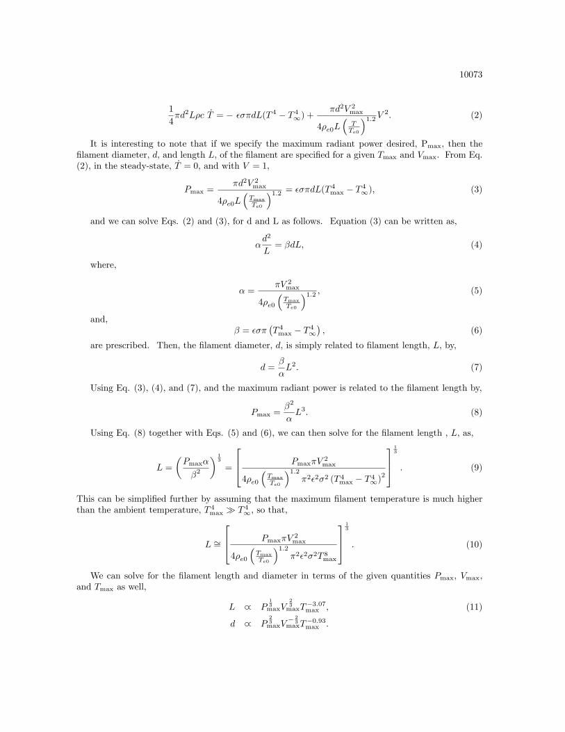
10073
1
4�d2L�c _T = � ���dL(T 4 � T 41) +
�d2V 2max
4�e0L�TTe0
�1:2V 2: (2)
It is interesting to note that if we specify the maximum radiant power desired, Pmax; then the�lament diameter, d, and length L, of the �lament are speci�ed for a given Tmax and Vmax: From Eq.(2), in the steady-state, _T = 0; and with V = 1,
Pmax =�d2V 2max
4�e0L�TmaxTe0
�1:2 = ���dL(T 4max � T 41); (3)
and we can solve Eqs. (2) and (3), for d and L as follows. Equation (3) can be written as,
�d2
L= �dL; (4)
where,
� =�V 2max
4�e0
�TmaxTe0
�1:2 ; (5)
and,� = ���
�T 4max � T 41
�; (6)
are prescribed. Then, the �lament diameter, d, is simply related to �lament length, L, by,
d =�
�L2: (7)
Using Eq. (3), (4), and (7), and the maximum radiant power is related to the �lament length by,
Pmax =�2
�L3: (8)
Using Eq. (8) together with Eqs. (5) and (6), we can then solve for the �lament length , L, as,
L =
�Pmax�
�2
� 13
=
264 Pmax�V2max
4�e0
�TmaxTe0
�1:2�2�2�2 (T 4max � T 41)
2
37513
: (9)
This can be simpli�ed further by assuming that the maximum �lament temperature is much higherthan the ambient temperature, T 4max � T 41; so that,
L �=
264 Pmax�V2max
4�e0
�TmaxTe0
�1:2�2�2�2T 8max
37513
: (10)
We can solve for the �lament length and diameter in terms of the given quantities Pmax, Vmax,and Tmax as well,
L _ P13maxV
23maxT
�3:07max ; (11)
d _ P23maxV
� 23
maxT�0:93max :

10074 CHAPTER 10. CONTROL-SYSTEM DESIGN: PRINCIPLES AND CASE STUDIES
Figures (a), (b), and (c) on top of the next page show plots of the functional relationship between�lament diameter and length as a function of the maximum power, Pmax, maximum temperature,Tmax, and maximum voltage, Vmax, respectively as well as the nominal operating point correspondingto Pmax = 200W , Tmax = 3000K, and , Vmax = 120V . Figure (a) shows that increasing Pmax requiresincreases in both the �lament diameter and length. As seen from Figure (b), increasing the maximumtemperature, Tmax, requires decreasing the �lament length but is relatively insensitive to the �lamentdiameter. Figure (c) shows that increasing the maximum voltage, Vmax, requires increasing the�lament length but decreasing the �lament diameter. Figures (a), (b), and (c) on the bottom of thenext page show the same relationships as in the top �gure but in terms of the normalized diameter,
ddnomin al
, and normalized �lament length, LLnomin al
.
0 500 10000
1
2
3
(a) Pmax
0 100 200 3000
2
4
6
(b) Vmax(V)
2000 2500 30000.5
1
1.5
2
(c) Tmax(K)0 500 1000
0
1
2
3
(a) Pmax
d [mm]L [m]
0 500 10000
1
2
3
(a) Pmax
0 100 200 3000
2
4
6
(b) Vmax(V)
d [mm]L [m]
0 500 10000
1
2
3
(a) Pmax
d [mm]L [m]
0 500 10000
1
2
3
(a) Pmax
0 100 200 3000
2
4
6
(b) Vmax(V)
2000 2500 30000.5
1
1.5
2
(c) Tmax(K)0 500 1000
0
1
2
3
(a) Pmax
d [mm]L [m]
0 500 10000
1
2
3
(a) Pmax
0 100 200 3000
2
4
6
(b) Vmax(V)
d [mm]L [m]
0 500 10000
1
2
3
(a) Pmax
d [mm]L [m]
d/dnominalL/Lnominal
Problem 10.20: Lamp design parametrs.

10075
0 500 10000
0.5
1
1.5
(a) Pmax(W)0 500 1000
0
0.5
1
1.5
(a) Pmax(W)
0 100 200 3000
0.5
1
1.5
(b) Vmax(V)
0 500 10000
0.5
1
1.5
(a) Pmax(W)0 500 1000
0
0.5
1
1.5
(a) Pmax(W)
0 100 200 3000
0.5
1
1.5
(b) Vmax(V)
2000 2500 30000
0.5
1
1.5
2
(c) Tmax(K)0 500 1000
0
0.5
1
1.5
(a) Pmax(W)0 500 1000
0
0.5
1
1.5
(a) Pmax(W)
0 100 200 3000
0.5
1
1.5
(b) Vmax(V)
0 500 10000
0.5
1
1.5
(a) Pmax(W)0 500 1000
0
0.5
1
1.5
(a) Pmax(W)
0 100 200 3000
0.5
1
1.5
(b) Vmax(V)
2000 2500 30000
0.5
1
1.5
2
(c) Tmax(K)
d [mm]L [m]
Problem 10.21: Lamp design parameters: normalized.
Assume the nominal operating temperature is denoted by T0. Re-writing Equation (2) in terms ofthe normalized temperature, we have
_T
T0
!= �4��T
30
�cd
"�T
T0
�4��T1T0
�4#+
V 2max4�e0�cL
2T0
V 2�TTe0
�1:2 : (12)
Let us de�ne the normalized temperature, x = TT0;and re-write Eq. (12) as the nonlinear �rst-order
system,
_x = �A(x4 � x41) +BV 2
x1:2; (13)
where,
A =4��T 30�cd
;
B =V 2max
4�e0�cL2T0
:
Linearizing Equation (13) about the nominal (normalized) temperature, we �nd the �rst-order

10076 CHAPTER 10. CONTROL-SYSTEM DESIGN: PRINCIPLES AND CASE STUDIES
linear dynamic model for the lamp as,
_x = �4Ax30x�B1:2
x2:20V 2; (14)
which means that the lamp time constant is,
� =1
4Ax30�=
�cd
16��T 30 x30
: (15)
In terms of lamp current, we have,
I =�d2Vmax
4�e0L�TTe0
�1:2V: (16)
Equation (15) implies that fast lamp response requires high �lament temperature and low �lamentdiameter. Typical values for the lamp �lament time constant range from 0.5 to 2 seconds.
The output of the lamp may be considered to be current, normalized �lament temperature, orradiative power,
ylamp =
24 Ix
Pmax
35 : (17)
A nonlinear simulation for the lamp model may be implemented in Simulink as shown on the nextpage. The results of the simulation show the temperature and current response of the lamp to a stepvoltage command input as shown. The �gure shows the fast lamp �lament temperature response witha time constant of 0.07 seconds, and also shows that the current initially surges but quickly drops toa steady-state within approximately 0.3 seconds.

10077
2O
ut21
Out
1
Icur
rent
To W
orks
pace
1
Tnor
m
To W
orks
pace
Icur
rent
.mat
To F
ile1
ToT.
mat
To F
ile
Ste
p
Sco
pe1
Sco
pe
Pro
duct
1
Pro
duct
1 uM
ath
Func
tion5
1 uM
ath
Func
tion4
uv
Mat
hFu
nctio
n3
uv
Mat
hFu
nctio
n2
uv
Mat
hFu
nctio
n1
uv
Mat
hFu
nctio
n
1 s
Inte
grat
orb Gai
n2
a
Gai
n1
K Gai
n
1.2
Con
stan
t4
2
Con
stan
t3
0.3
Con
stan
t2
4
Con
stan
t1
4
Con
stan
t
Problem 10.21: Simulink diagram for lamp model.

10078 CHAPTER 10. CONTROL-SYSTEM DESIGN: PRINCIPLES AND CASE STUDIES
0 0.1 0.2 0.3 0.4 0.50
2
4
6
8
10
12
14
Time (sec)
Fila
men
t tem
pera
ture
, cur
rent
Response to s tep voltage command
0 0.1 0.2 0.3 0.4 0.50
2
4
6
8
10
12
14
Problem 10.21: Lamp response to a step voltage command.
References:[1] Reynolds, W. C., and H. C. Perkins, Engineering Thermodynamics, McGraw-Hill, 1977.[2] A. Emami-Naeini, et al., �Modeling and Control of Distributed Thermal Systems,�IEEE Tran.
Contrl. Syst. Tech., pp. 668-683, September 2003.[3] Lide, D. R., Ed., Handbook of Chemistry and Physics, CRC Press, 1993-1994.[4] Modest, M. F., Radiative Heat Transfer, McGraw-Hill, 1993.22. Develop a nonlinear model for a pyrometer. Show how temperature can be deduced from the
model.Solution:Temperature measurement can be done by a variety of methods including thermocouples, resistive
temperature detectors (RTDs), and pyrometers [1]. A pyrometer is a non-contact temperature sensorand measures the Infrared (IR) radiation which is directly a function of the temperature. It isknown that objects emit radiant energy proportional to T 4 where T is the temperature of the object.Among the advantages of pyrometers are that they have very fast response time, can be used tomeasure the temperature of moving objects (e.g., a rotating semiconductor wafer), and in vacuum forsemiconductor manufacturing.The single-wavelength pyrometer measures the total energy emitted from a surface at a given
wavelength. To understand the operation of a pyrometer, we need to review some concepts fromradiation heat transfer [2-3]. The emissivity of an object, �, is de�ned as the ratio of the energy �uxemitted by a surface to that from a black body at the same temperature:

10079
� =
R��Ib�(T )d�RIb�(T )d�
; (18)
where,
� = total emissivity,
�� = spectral emissivity,
T = absolute temperature, K;
� = wavelength of radiation, �m;
Ib� = spectral black body intensity.
The frequency, �, is given by,
� =c0�0;
where,
c0 = speed of light in vacuum = 2:998� 108m=s;�0 = wavelength of light in vacuum.
The Plank�s law of radiation states that the spectral radiance of a blackbody, or spectral intensity,Ib� , in a dielectric medium as a function of the wavelength and temperature is,
Ib�(T ) =2h�3n2
c2o(eh�kT � 1)
; (19)
where,
h = Planck0s constant = 6:626� 10�34Js;k = Boltzmann0s constant = 1:3806� 10�23J=K;n = real refractive index (n = 1 for most gases),
and the frequency and wavelength are related by,
� =c
�; (20)
where c is the speed of light in the medium and is given by,
c =c0n:
After some manipulation, we can re-write Eq. (19) as [2],
Ib�(T ) =2hc20
n2�5(ehc0n�kT � 1)
: (21)

10080 CHAPTER 10. CONTROL-SYSTEM DESIGN: PRINCIPLES AND CASE STUDIES
The total black-body radiation intensity, Ib, is obtained by integrating over all frequencies orwavelength [2]
Ib(T ) =
ZI�b(T )d� (22)
=n2�T 4
�:
The black body emissive �ux is given by,
q�b(T ) =C1
n2�5(eC2n�T � 1)
; (23)
where,
C1 = 2�hc20 = 3:7419� 10�16; W=m2; (24)
C2 =hc0k= 14388 �mK:
Integrating over all wavelengths �, we obtain the total black body emissive �ux [2],
qb(T ) =
Z 1
0
q�b(T )d� (25)
= n2�T 4;
where � is the Stefan-Boltzman constant, � = 5:67� 10�8 W=(m2K4):
The temperature may be determined from Eq. (19) as,
T =C2�
1
ln(1 + ��CI )
; (26)
where,
C =C1
�5: (27)

10081
Problem 10.22: Schematic of temperature measurement using pyrometry.
The �gure on the bottom of the previous page shows the schematic of temperature measurementof a semiconductor wafer using pyrometry where, for this particular application, response time andview angle are very important. A two color pyrometer is also used for applications where absolutetemperature measurement is important. The measurement can then be used for feedback controlpurposes, e.g., pyrometers are now routinely used in control of rapid thermal processing (RTP) systemsin semiconductor manufacturing [4].References:[1] Fraden, J., Handbook of Modern sensors: Physics, Designs, and Applications, Springer, 1996.[2] Ozisik, M. N., Radiative Transfer and Interactions with Conduction and Convection, Wiley-
Interscience, 1973.[3] Siegel, R. and J. R. Howell, Thermal Radiation Heat Transfer, Second Ed., Hemisphere Pub-
lishing Corp., 1981.[4] A. Emami-Naeini, et al., �Modeling and Control of Distributed Thermal Systems,�IEEE Tran.
Contrl. Syst. Tech., pp. 668-683, September 2003.23. Repeat the RTP case study design by summing the three sensors to form a single signal to
control the average temperature. Demonstrate the performance of the linear design, and validate theperformance on the nonlinear Simulink simulation.Solution:A linear model for the system was derived in the text as,
_T = F3 T+G3 u; (28)
y = H 3T+ J3 u;
where y = [Ty1 Ty2 Ty3]T and,
F3 =
24 �0:0682 0:0149 0:00000:0458 �0:1181 0:02180:0000 0:04683 �0:1008
35 ; G3 =
24 0:3787 0:1105 0:02290:0000 0:4490 0:07350:0000 0:0007 0:4177
35 ;

10082 CHAPTER 10. CONTROL-SYSTEM DESIGN: PRINCIPLES AND CASE STUDIES
H3 =
24 1 0 00 1 00 0 1
35 ; J3 =
24 0 0 00 0 00 0 0
35 :
The three open-loop poles are computed from Matlab and are located at �0:0527;�0:0863; and�0:1482: Since we tied the three lamps into one actuator and are only using the average temperaturefor feedback, the linear model is then:
F =
24 �0:0682 0:0149 0:00000:0458 �0:1181 0:02180:0000 0:04683 �0:1008
35 ; G =
24 0:51220:52260:4185
35 ;
Havg =�13
13
13
�; J = [0] ;
resulting in the transfer function,
G(s) =Tyavg(s)
Vcmd(s)=
0:4844(s+ 0:0878)(s+ 0:1485)
(s+ 0:1482)(s+ 0:0527)(s+ 0:0863):
We may try a simple PI controller of the form,
Dc(s) =(s+ 0:0527)
s;
so as to cancel the e¤ect of the slower pole. The linear closed-loop response is shown as well as theassociated control e¤ort The system response follows the commanded trajectory with a time delayof approximately 2 sec and no overshoot. The lamp has its normal response until 75 sec and goesnegative (shown in dashed) to try to follow the sharp drop in commanded temperature. As mentionedin the text, this behavior is not possible in the system as there is no means of active cooling and thelamps do saturate low. There is no explicit means of controlling the temperature nonuniformity usingthe PI controller.

10083
0 20 40 60 80 1005
0
5
10
15
20
25
30
Time (sec)
Tem
pera
ture
(K)
PID (average) temperature tracking response
0 20 40 60 80 1005
0
5
10
15
20
25
30
Time (sec)
Tem
pera
ture
(K)
PID (average) temperature tracking response
ry
Problem 10.23: Linear closed-loop RTP response for PI controller.

10084 CHAPTER 10. CONTROL-SYSTEM DESIGN: PRINCIPLES AND CASE STUDIES
0 20 40 60 80 10025
20
15
10
5
0
5
Time (sec)
Lam
p vo
ltage
(V)
PID (average) temperature : control effort
0 20 40 60 80 10025
20
15
10
5
0
5
Problem 10.23: RTP Linear response for PI: control e¤ort.
Next we design a state-space based controller. As in the text, we use the error space approach forinclusion of integral control and employ the linear quadratic gaussian technique of Chapter 7. Theerror system is, �
_e_�
�=
�0 Havg
0 F
� �e�
�+
�JG
��; (29)
where,
A =
�0 Havg
0 F
�;B =
�JG
�:
and e = y � r; � = _T with � = _u. For state feedback design, the LQR formulation of Chapter 7is used
J =
Z 1
0
fzTQ z+��2gdt;
where z =[e �T ]T : Note that J has been chosen in such a way as to penalize the tracking error, e,the control, u, as well as the di¤erences in the three temperatures�therefore, the performance indexshould include a term of the form,
10�(T1 � T2)2 + (T1 � T3)2 + (T2 � T3)2
;

10085
and hence minimizes the temperature non-uniformity. As in the text, the factor of ten is used asthe relative weighting between the error state and the plant state. The state and control weightingmatrices, Q and R, are then,
Q =
26641 0 0 00 20 �10 �100 �10 20 �100 �10 �10 20
3775 ; R = � = 1:
The following Matlab command is used to design the feedback gain,[K]=lqr(A,B,Q,R).
The resulting feedback gain matrix computed from Matlab is,
K = [K1 : K0];
where,
K1 = 1; K0 =�0:7344 0:9344 0:3921
�;
which results in the internal model controller of the form,
_xc = Bc e; (30)
u = Cc xc �K0 T;
with xc denoting the controller state and,
Bc = �K1 = �1; Cc = 1:
The resulting state-feedback closed-loop poles computed using Matlab�s eig command are at�0:5395 � 0:4373j;�0:1490; and �0:0879. The full-order estimator was designed with the sameprocess and sensor noise intensities used in the text as the estimator design knobs,
Rw = 1; Rv = 0:001:
The following Matlab command is used to design the estimator,[L]=lqe(F,G,H,Rw,Rv).
The resulting estimator gain matrix is,
L =
24 16:14216:466713:1975
35 ;with estimator error poles at �15:3197;�0:1485; and �0:0878: The estimator equation is,
_T = FT+Gu+L(y�HT): (31)
With the estimator, the internal model controller equation is modi�ed as in the text
_xc = Bc e; (32)
u = Cc xc �K0 T:

10086 CHAPTER 10. CONTROL-SYSTEM DESIGN: PRINCIPLES AND CASE STUDIES
The closed-loop system equations are given in the text,
_xcl = Acl xcl +Bcl r; (33)
y = Ccl xcl +Dcl r;
where r is the reference input temperature trajectory, the closed-loop state vector is xcl = [TT xTc TT]T and
the system matrices are,
Acl =
24 F GCc �GK0
BcH 0 0LH GCc F�GK0�LH
35 ; Bcl =
24 0�Bc0
35 ;Ccl =
�H 0 0
�; Dcl = [0];
with closed-loop poles (computed with Matlab) located at �0:5395� 0:4373j;�0:1490; �0:0879;
�15:3197;�0:1485 and �0:0879 as expected. The closed-loop control structure is as shown in textFigure 10.85.
The linear closed-loop response and the associated control e¤ort are shown. The commandedtemperature trajectory, r, is a ramp from 0�C to 25�C with a 1�C/sec slope followed by 50 sec soaktime and drop back to 0�C. The system tracks the commanded temperature trajectory �albeit witha time delay of approximately 2 seconds for the ramp and a maximum of 0:0216�C overshoot. Asexpected the system tracks a constant input asymptotically with zero steady-state error. The lampcommand increases as expected to allow for tracking the ramp input, reaches a maximum value at25 sec and then drops to a steady-state value around 35 sec. The normal response of the lamp isseen from 0 to 75 sec followed by negative commanded voltage for a few seconds corresponding to fastcooling. Again, the negative control e¤ort voltage (shown in dashed lines) is physically impossible asthere is no active cooling in the system. Hence in the nonlinear simulations, commanded lamp powermust be constrained to be strictly non-negative. Note that the response from 75� 100 sec is that ofthe (negative) step response of the system.

10087
0 20 40 60 80 1005
0
5
10
15
20
25
30
Time (sec)
tem
pera
ture
(K)
temperature tracking response
0 20 40 60 80 1005
0
5
10
15
20
25
30ry
Problem 10.23: RTP linear (average) temperature tracking response.

10088 CHAPTER 10. CONTROL-SYSTEM DESIGN: PRINCIPLES AND CASE STUDIES
0 20 40 60 80 10014
12
10
8
6
4
2
0
2
4
6
Time (sec)
lam
p vo
ltage
control effort
u
0 20 40 60 80 10014
12
10
8
6
4
2
0
2
4
6
Time (sec)
lam
p vo
ltage
control effortu
Problem 10.23 RTP linear (average) : control e¤ort.
The nonlinear closed-loop system was simulated in Simulink as shown on the next page. In thediagram, Gain4 =
�13
13
13
�. As in the text, the model was implemented in temperature units of
degrees Kelvin and the ambient temperature is 301K. The nonlinear plant model is the implementa-tion of text Eq. 10.48. The voltage range for system operation is between 1 to 4 volts as seen fromthe diagram. As in the text, a saturation nonlinearity is included for the lamp as well as integratoranti-windup logic to deal with lamp saturation. The nonlinear dynamic response and the controle¤ort are shown. Note that the nonlinear response is in general agreement with the linear response.

10089
ko
k1N
onlin
ear P
lant
InvL
amp
Vto
Pow
er
Est
imat
orLam
pU
ncer
tain
ty
Ant
iwin
dup
yavg
To W
orks
pace
3
u
To W
orks
pace
2
r
To W
orks
pace
1
y
To W
orks
pace
In1
Out
1
Sub
syst
em2
In1
Out
1
Sub
syst
em1
In1
Out
2
Sub
syst
em
x' =
Ax+
Bu
y =
Cx+
Du
Sta
teS
pace
1
Sco
pe5
Sco
pe4
Sco
pe3
Sco
pe2
Sco
pe1
Sco
peS
atur
atio
nR
epea
ting
Seq
uenc
e
K*u Mat
rixG
ain5
K*u
Mat
rixG
ain4
K*u Mat
rixG
ain3
K*u
Mat
rixG
ain2
K*u Mat
rixG
ain1
K*u
Mat
rixG
ain
1 s
Inte
grat
or
Problem 10.23: Simulink diagram for nonlinear closed-loop RTP system to control averagetemperature.

10090 CHAPTER 10. CONTROL-SYSTEM DESIGN: PRINCIPLES AND CASE STUDIES
20 40 60 80 100 120 140 160 180310
315
320
325
330
335
Time (sec)
Tem
pera
ture
(K)
SISO (average) temperature tracking response
ry
20 40 60 80 100 120 140 160 180310
315
320
325
330
335
Time (sec)
Tem
pera
ture
(K)
SISO (average) temperature tracking responsery
Problem 10.23: Nonlinear closed-loop response.

10091
20 40 60 80 100 120 140 160 1800
0.5
1
1.5
2
2.5
3
3.5
4
Time (sec)
Lam
p vo
ltage
(V)
SISO (average) temperature : control effort
20 40 60 80 100 120 140 160 1800
0.5
1
1.5
2
2.5
3
3.5
4
Problem 10.23: Nonlinear closed-loop response: control e¤ort.
24. One of the steps in semiconductor wafer manufacturing during photolithography is performedby placement of the wafer on a heated plate for a certain period of time. Laboratory experimentshave shown that the transfer function from the heater power, u, to the wafer temperature, y, is givenby
y(s)
u(s)= G(s) =
0:09
(s+ 0:19)(s+ 0:78)(s+ 0:00018)
1. (a) Sketch the 180� root locus for the uncompensated system.
(b) Using the root locus design techniques, design a dynamic compensator, D(s), such thatthe system meets the following time-domain speci�cations
i. Mp � 5%ii. tr � 20 seciii. ts � 60 seciv. Steady-state error to a 1�C step input command < 0:1�C.
Draw the 180� root locus for the compensated system.
Solution:
The uncompensated root locus is shown in the following �gure.

10092 CHAPTER 10. CONTROL-SYSTEM DESIGN: PRINCIPLES AND CASE STUDIES
3.5 3 2.5 2 1.5 1 0.5 0 0.5 1 1.52.5
2
1.5
1
0.5
0
0.5
1
1.5
2
2.5
0.94
0.985
0.160.340.50.640.76
0.86
0.94
0.985
0.511.522.533.5
0.160.340.50.640.76
0.86
Root Locus
Real Axis
Imag
inar
y Ax
is
Uncompensated root locus.
(a) First, convert the time domain speci�cations to s-plane speci�cations:
Mp � 5%) & > 0:707tr � 20 sec) !n > 0:09ts � 60 sec) � > 0:0767
(b) At this point there are several design methods one can use for this problem.Method I: We know that a pure integrator will improve steady-state behavior and wenearly have a pure integrator with the pole at -0.00018. Thus, we can cancel another(stable) pole with a lead network zero, and place a fast lead pole to appropriately shapethe root locus. One possible lead compensator is
D(s) = Kcs+ 0:19
s+ 1
We can display the compensated root locus and s-plane regions in RLTool in the fol-lowing �gure.

10093
RLTool: Compensator I.
Choosing Kc = 2 gives us the closed-loop poles within the speci�cations at s = �0:24�j0:28. The results from RLTool follows.

10094 CHAPTER 10. CONTROL-SYSTEM DESIGN: PRINCIPLES AND CASE STUDIES
Step Response
Time (sec)
Ampl
itude
0 5 10 15 20 250.5
0
0.5
1
1.5
2
0 5 10 15 20 250.5
0
0.5
1
1.5
2
RLTool: Step response (y) and control e¤ort (u) for Compensator I.
Method II: We can cancel out the nearly pure integrator with our compensator zero, andadd a pure integrator. It is possible to achieve the time domain speci�cations with thiscompensator. The compensator becomes
D(s) = Ks+ 0:00018
s
Applying the magnitude condition with the desired poles at s = �008� j0:08, we get
K = 0:12
We can display the compensated root locus and s-plane regions in RLTool in the following�gure.

10095
RLTool: Compensator II.

10096 CHAPTER 10. CONTROL-SYSTEM DESIGN: PRINCIPLES AND CASE STUDIES
Step Response
Time (sec)
Ampl
itude
0 10 20 30 40 50 60 700.2
0
0.2
0.4
0.6
0.8
1
1.2
0 10 20 30 40 50 60 700.2
0
0.2
0.4
0.6
0.8
1
1.2
RLTool: Step response (y) and control e¤ort (u) for Compensator II.
25. Excitation-Inhibition Model from Systems Biology (Yang and Iglesias, 2005): In Dictyosteliumcells, the activation of key signaling molecules involved in chemoattractant sensing can be modeled bythe following third order linearized model. The external disturbance to the output transfer functionis:
y(s)
w(s)= S(s) =
(1� �)s(s+ �)(s+ 1)(s+ )
where, w is the external disturbance signal proportional to chemoattractant concentration, and yis the output which is the fraction of active response regulators. Show that there is an alternaterepresentation of the system with the �plant�transfer function
G(s) =(1� �)
s2 + (1 + �+ )s+ (�+ + � )
and the �feedback regulator�D(s) =
�
(1� �)sIt is known that � 6= 1 for this version of the model. Draw the feedback block diagram of thesystem showing the locations of the disturbance input and the output. What is the signi�cance ofthis particular representation of the system? What hidden system property does it reveal? Is thedisturbance rejection a robust property for this system? Plot the disturbance rejection response of

10097
the system for a unit step disturbance input. Assume the system parameter values are � = 0:5 and = 0:2.
1. Solution: From the following �gure we have
Feedback loop representation.
Y (s)
W (s)=
(1��)s2+(1+�+ )s+(�+ +� )
1 + (1��)s2+(1+�+ )s+(�+ +� )
� (1��)s
=(1� �)s
(s+ �)(s+ 1)(s+ )
The signi�cance of this particular representation is that it reveals the internal model, namelythe pure integrator. Hence the system is Type I with respect to disturbance rejection. It rejectsconstant disturbances in a robust fashion. For � = 0:5 and = 0:2, we have
G(s) =0:5s
s2 + 1:7s+ 0:8
The disturbance response is shown in the following �gure.

10098 CHAPTER 10. CONTROL-SYSTEM DESIGN: PRINCIPLES AND CASE STUDIES
0 1 2 3 4 5 6 7 8 9 100
0.05
0.1
0.15
0.2
0.25
Step Response
Time (sec)
Ampl
itude
0 1 2 3 4 5 6 7 8 9 100
0.05
0.1
0.15
0.2
0.25
Disturbance rejection response for a unit step disturbance.