Engineering Exact Quasi-Threshold EditingLars GottesbürenInstitute of Theoretical Informatics, Karlsruhe Institute of Technology, Karlsruhe, Germanylars.gottesbueren@kit.edu

Michael HamannInstitute of Theoretical Informatics, Karlsruhe Institute of Technology, Karlsruhe, Germanymichael.hamann@kit.edu

Philipp SchochInstitute of Theoretical Informatics, Karlsruhe Institute of Technology, Karlsruhe, Germany

Ben StrasserInstitute of Theoretical Informatics, Karlsruhe Institute of Technology, Karlsruhe, Germanyacademia@ben-strasser.net

Dorothea WagnerInstitute of Theoretical Informatics, Karlsruhe Institute of Technology, Karlsruhe, Germanydorothea.wagner@kit.edu

Sven ZühlsdorfInstitute of Theoretical Informatics, Karlsruhe Institute of Technology, Karlsruhe, Germanyzuehlsdorf.kit@ghostdub.de

AbstractQuasi-threshold graphs are {C4, P4}-free graphs, i.e., they do not contain any cycle or path of fournodes as an induced subgraph. We study the {C4, P4}-free editing problem, which is the problemof finding a minimum number of edge insertions or deletions to transform an input graph into aquasi-threshold graph. This problem is NP-hard but fixed-parameter tractable (FPT) in the numberof edits by using a branch-and-bound algorithm and admits a simple integer linear programmingformulation (ILP). Both methods are also applicable to the general F-free editing problem forany finite set of graphs F . For the FPT algorithm, we introduce a fast heuristic for computinghigh-quality lower bounds and an improved branching strategy. For the ILP, we engineer severalvariants of row generation. We evaluate both methods for quasi-threshold editing on a large setof protein similarity graphs. For most instances, our optimizations speed up the FPT algorithmby one to three orders of magnitude. The running time of the ILP, that we solve using Gurobi,becomes only slightly faster. With all optimizations, the FPT algorithm is slightly faster than theILP, even when listing all solutions. Additionally, we show that for almost all graphs, solutions ofthe previously proposed quasi-threshold editing heuristic QTM are close to optimal.

2012 ACM Subject Classification Information systems → Clustering; Theory of computation →Graph algorithms analysis; Theory of computation → Fixed parameter tractability; Theory ofcomputation → Branch-and-bound

Keywords and phrases Edge Editing, Integer Linear Programming, FPT algorithm, Quasi-ThresholdEditing

Supplement Material Implementation: https://github.com/kit-algo/fpt-editing

Funding This work was supported by the Deutsche Forschungsgemeinschaft (DFG, German ResearchFoundation) under grants WA654/19-2 and WA654/22-2. The authors acknowledge support by thestate of Baden-Württemberg through bwHPC.

Acknowledgements We thank James Nastos and Mark Ortmann for helpful discussions.

arX

iv:2

003.

1431

7v1

[cs

.DS]

31

Mar

202

0

2 Engineering Exact Quasi-Threshold Editing

(a) A C4. (b) A P4.

b

c

d

a e

(c) A graph with node-induced C4.

d e f

a b c

(d) A {C4, P4}-free graph.

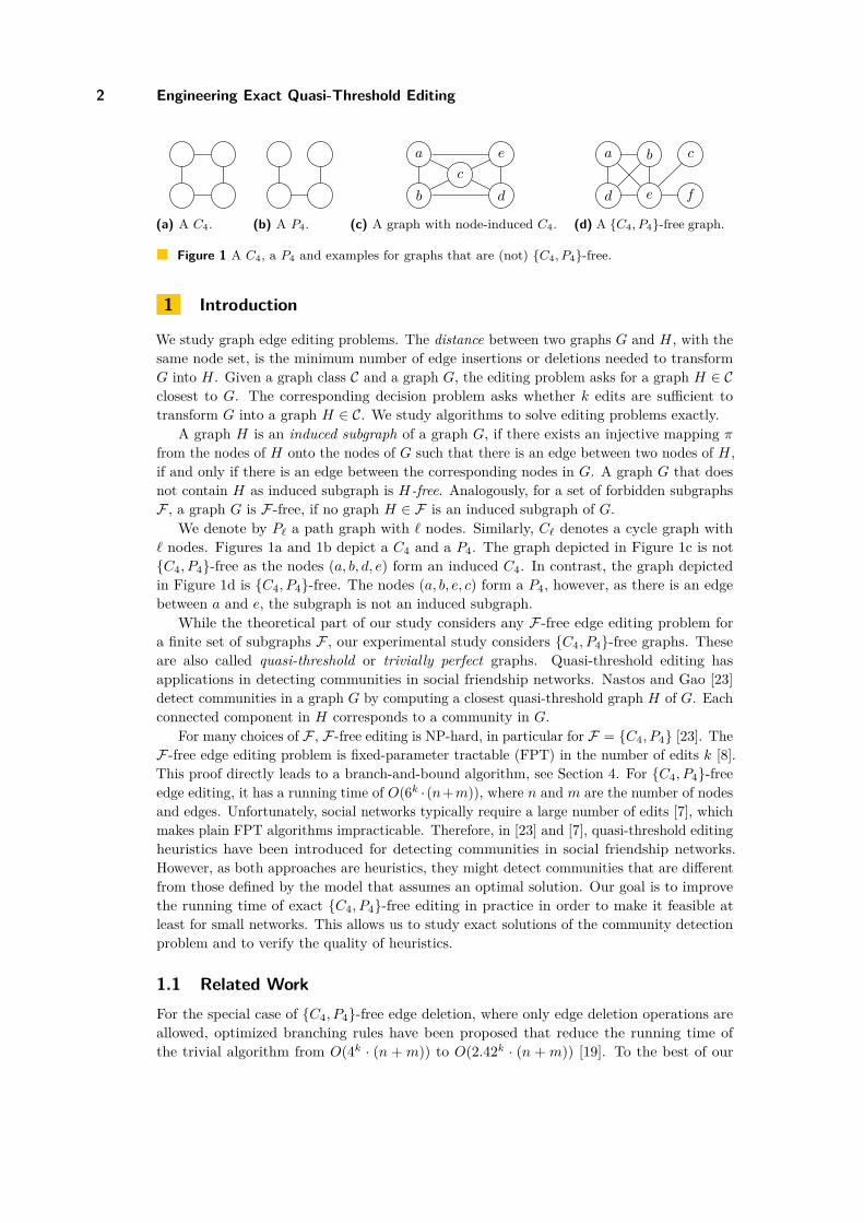
Figure 1 A C4, a P4 and examples for graphs that are (not) {C4, P4}-free.

1 Introduction

We study graph edge editing problems. The distance between two graphs G and H, with thesame node set, is the minimum number of edge insertions or deletions needed to transformG into H. Given a graph class C and a graph G, the editing problem asks for a graph H ∈ Cclosest to G. The corresponding decision problem asks whether k edits are sufficient totransform G into a graph H ∈ C. We study algorithms to solve editing problems exactly.

A graph H is an induced subgraph of a graph G, if there exists an injective mapping πfrom the nodes of H onto the nodes of G such that there is an edge between two nodes of H,if and only if there is an edge between the corresponding nodes in G. A graph G that doesnot contain H as induced subgraph is H-free. Analogously, for a set of forbidden subgraphsF , a graph G is F-free, if no graph H ∈ F is an induced subgraph of G.

We denote by P` a path graph with ` nodes. Similarly, C` denotes a cycle graph with` nodes. Figures 1a and 1b depict a C4 and a P4. The graph depicted in Figure 1c is not{C4, P4}-free as the nodes (a, b, d, e) form an induced C4. In contrast, the graph depictedin Figure 1d is {C4, P4}-free. The nodes (a, b, e, c) form a P4, however, as there is an edgebetween a and e, the subgraph is not an induced subgraph.

While the theoretical part of our study considers any F-free edge editing problem fora finite set of subgraphs F , our experimental study considers {C4, P4}-free graphs. Theseare also called quasi-threshold or trivially perfect graphs. Quasi-threshold editing hasapplications in detecting communities in social friendship networks. Nastos and Gao [23]detect communities in a graph G by computing a closest quasi-threshold graph H of G. Eachconnected component in H corresponds to a community in G.

For many choices of F , F -free editing is NP-hard, in particular for F = {C4, P4} [23]. TheF -free edge editing problem is fixed-parameter tractable (FPT) in the number of edits k [8].This proof directly leads to a branch-and-bound algorithm, see Section 4. For {C4, P4}-freeedge editing, it has a running time of O(6k · (n+m)), where n and m are the number of nodesand edges. Unfortunately, social networks typically require a large number of edits [7], whichmakes plain FPT algorithms impracticable. Therefore, in [23] and [7], quasi-threshold editingheuristics have been introduced for detecting communities in social friendship networks.However, as both approaches are heuristics, they might detect communities that are differentfrom those defined by the model that assumes an optimal solution. Our goal is to improvethe running time of exact {C4, P4}-free editing in practice in order to make it feasible atleast for small networks. This allows us to study exact solutions of the community detectionproblem and to verify the quality of heuristics.

1.1 Related WorkFor the special case of {C4, P4}-free edge deletion, where only edge deletion operations areallowed, optimized branching rules have been proposed that reduce the running time ofthe trivial algorithm from O(4k · (n + m)) to O(2.42k · (n + m)) [19]. To the best of our

L. Gottesbüren, M. Hamann, P. Schoch, B. Strasser, D. Wagner and S. Zühlsdorf 3

knowledge, for {C4, P4}-free editing, no improved branching rules have been proposed so far.A polynomial kernel of size O(k7) for {C4, P4}-free graphs has been proposed [12], which istoo large for most practical applications.

A frequently considered problem is {P3}-free editing, better known as cluster editing [2].Early approaches for cluster editing include a linear programming formulation with cuttingplanes that are incrementally added (in batches of a few hundred constraints) [14]. Later,exact algorithms based on integer linear programming as well as kernelization and moreefficient FPT algorithms have been considered [5]. In [16], the authors combine the FPTalgorithm with kernelization as well as upper and lower bounds. Editing to {P4}-free graphshas been considered in phylogenomics [17] using a simple ILP-based approach.

In a bachelor thesis [6], {P5}-free editing has been considered for community detection.They apply lower bounds, data reduction rules and rules for disallowing certain edits.

1.2 Our ContributionIn this paper, we compare two different methods for solving F -free editing problems. The firstis a branch-and-bound FPT algorithm while the second is an ILP. For the FPT algorithm, wepropose a novel lower bound algorithm based on local search heuristics for independent setsas well as an improved branching strategy. Additionally, we parallelize our implementation.For the ILP, we engineer several variants of row generation. We assess the running timeimprovements of the different optimizations for quasi-threshold editing on a large benchmarkset of 716 graphs that are connected components of a protein similarity graph. This benchmarkset has previously been used to evaluate cluster editing algorithms [24, 3]. On 75% of theinstances, our improved bounds and optimized branching choices yield speedups of one tothree orders of magnitude for the FPT algorithm. For the ILP, we are only able to achievesmall speedups. With all optimizations, in the median, the FPT algorithm is twice as fastas the ILP, even when enumerating all possible optimal solutions exactly once. Comparedwith the parallel execution of Gurobi [15], the FPT algorithm achieves better speedups.Additionally, we evaluate an LP relaxation as lower bound. We prove that its bounds are atleast as good as our local search bounds. In our experiments, however, it is too slow to becompetitive.

Further, we compare our exact solutions with heuristic solutions found by QTM [7].It turns out that many heuristic solutions are exact and all but one of them are close tothe exact solution. Additionally, we are able to solve four out of the five social networksconsidered in [23], of which only one was solved previously [21].

1.3 OutlineWe start by introducing the preliminaries in Section 2. We describe the ILP formulationand the optimizations we apply to it in Section 3. In Section 4, we then introduce thebranch-and-bound FPT algorithm including existing and novel optimizations. In Section 5,we present our experimental setup and evaluation. We conclude in Section 6.

2 Preliminaries

All graphs in this paper are undirected, unweighted, and finite. Further, no graph hasself-loops or multi-edges. A graph G = (VG, EG) consists of n := |VG| nodes and m := |EG|undirected edges. By EG, we denote the complement of the edges. In the following, k denotesthe maximum number of edits.

4 Engineering Exact Quasi-Threshold Editing

3 Integer Linear Programming

In this section, we describe an ILP formulation for F -free editing that is based on an existingformulation for cluster editing [14]. Further, we introduce our optimizations based on rowgeneration and modified constraints to make the ILP practical for small instances.

For every node pair u, v ∈(VG

2)we introduce a variable xuv ∈ {0, 1} which is 1 if the

node pair is an edge in the edited graph and 0 otherwise. We add constraints to ensure thatno forbidden subgraph H ∈ F can be induced in G via an injective node mapping π:

∀H ∈ F ,∀π : VH ↪→ VG :∑

{u,v}∈EH

(1− xπ(u)π(v)) +∑

{u,v}∈EH

xπ(u)π(v) ≥ 1 (1)

The objective minimizes the number of edits:

min∑

{u,v}∈EG

(1− xuv) +∑

{u,v}∈EG

xuv (2)

3.1 Row GenerationGenerating all of the above-mentioned constraints is infeasible, even for small instances. Rowgeneration (also called lazy constraints) aims to speed up ILP solvers by starting with asmall subset of the constraints and subsequently adding constraints that are violated inintermediate solutions. We start with constraints for forbidden subgraphs in the input graph.In our experiments, we consider two options to add constraints violated in an intermediatesolution: adding either all violated constraints or only one.

The ILP solver uses LP relaxations to prune its search. These can be strengthened byadding constraints from Equation 1 that are violated by the LP relaxation. We generateconstraints in three steps. First, we consider each node pair {u, v} for which the relaxationsolution has a value different from the input graph. We edit it, then enumerate the forbiddensubgraph embeddings containing u and v, add the constraint that is most violated (i.e.,whose left side is furthest below 1) and then revert the edit. Ties are broken uniformly atrandom. Second, we apply the same procedure to the best heuristic solution found so far.Third, we round the LP solution, i.e., an edge exists iff the corresponding variable is greaterthan 0.5. We then list forbidden subgraph embeddings in this rounded solution and add thecorresponding most violated constraint if there is any. The listing skips forbidden subgraphsfor which the corresponding constraint has already been added.

3.2 Optimizing Constraints for {C4, P4}-free EditingIf one forbidden subgraph can be transformed into another by a single edit, we can omit anode pair from the constraint for this subgraph. This is similar to the optimization describedin Section 4.2. For a P4, this is the node pair consisting of the two degree-one nodes. For aC4, we can omit any one of its four edges. We always consider all four possibilities, and inthe initial constraint generation as well as the basic row generation variant we add all ofthem. With this optimization, the constraints for C4s and P4s are identical.

We can also formulate a constraint for a C4 that explicitly models that two deletions orone insertion are required:

∀(u1, u2, u3, u4) ∈ V 4G : 0.5 ·

4∑i=1

(1− xuiui+1) + xu1u3 + xu2u4 ≥ 1 (3)

L. Gottesbüren, M. Hamann, P. Schoch, B. Strasser, D. Wagner and S. Zühlsdorf 5

4 The FPT Branch-and-Bound Algorithm

The FPT algorithm [8] is a branch-and-bound algorithm. For a given maximum number ofedits k, it either reports that no solution exists or returns a set of k edits. It works as follows:Find a forbidden subgraph H and branch on all possible edits in H. As H is induced, onlyedits in H can destroy it and thus one of these edits must be part of the solution. Thealgorithm is then recursively called for each branch with k − 1 remaining edits.

Denote by p the maximum number of nodes in a forbidden subgraph. Finding H can bedone trivially in time O(np) by enumerating all subgraphs of the required size. For specificsets of forbidden subgraphs, such as {C4, P4}, this can be improved to O(n+m) [9, 7].

Every pair of nodes in H is a valid edit. The branching factor is therefore p · (p− 1)/2.The depth of the recursion is bounded by the maximum number of edits k. The total runningtime is therefore in O(p2k ·np) for general families of forbidden subgraphs. For quasi-thresholdediting the running time is O(6k · (n + m)). This can be improved to O(5k · (n + m)) byapplying the optimization described in Section 4.2.

For finding the minimum number of edits kopt, the algorithm needs to be executed forincreasing values of k until a solution is returned. For a branching factor of 2 or larger, therunning time of all k < kopt together is at most the running time for kopt. Thus the totalrunning time is dominated by the running time for kopt.

In the following, we describe several optimizations to reduce the number of exploredbranches in practice. We describe existing techniques for avoiding redundant exploration ofbranches (Section 4.1), for skipping certain branches (Section 4.2) as well as lower bounds(Section 4.3). We introduce a novel local search lower bound (Section 4.4), optimized branchingchoices (Section 4.5), early pruning of branches (Section 4.6) and a simple parallelization(Section 4.7). In Appendix B we provide in-depth implementation details.

4.1 Avoiding RedundancyDamaschke [10] proposes to block node pairs to list every solution exactly once. Whenspawning a search tree node x through editing a node pair, it is neither useful to undo thatedit in the sub-search-tree rooted at x, nor is it useful to perform the edit in sibling searchtrees. While this has been introduced for cluster editing, the technique can be applied toarbitrary F-free editing problems. In Appendix A, we explain this technique in detail.

4.2 Skip Forbidden Subgraph Conversion.I Lemma 1. If each forbidden subgraph A ∈ F can be transformed into another one B ∈ Fby one edit, the branching factor of the FPT algorithm can be reduced from

(p2)

to(p2)− 1.

There is an edit that transforms a P4 into a C4. Clearly, this edit can be skipped. Further,there are four edge deletions that transform a C4 into a P4. One of these can be skipped [22].We can choose which one, but as any pair of two edge deletions eliminates the forbiddensubgraph, skipping more than one of them might eliminate a necessary branch. Since thebranching factor is reduced, this decreases the worst-case running time from O(6k · (n+m))to O(5k · (n+m)) for quasi-threshold editing.

4.3 Existing Lower Bound ApproachesAt each branching node, we have a certain number k of edits left. If we can show that thegraph needs at least k + 1 edits, we do not need to explore further branches below that node.

6 Engineering Exact Quasi-Threshold Editing

Lower bounds have been used for cluster editing [5, 16] and {P5}-free editing [6]. Commonly,they are based on an LP relaxation of the ILP [16], or on a disjoint packing argument [6, 16].

Subgraph Packing. A node-pair disjoint subgraph packing P is a set of induced forbiddensubgraphs that do not share a node pair. As no edit can eliminate more than one subgraph,|P | is a lower bound on the number of edits required. Taking the previously mentionedoptimizations into account, we can include more subgraphs in P by allowing to share blockednode pairs, as they cannot be edited. Further, for each forbidden subgraph a node pair thattransforms it into another forbidden subgraph may be shared. In the case of F = {C4, P4},the pair of degree-1 nodes of an induced P4 can be shared. For C4, we can choose any edgeto share, but it remains the same as long as the C4 is in the packing.

Finding such a packing can be modeled as an independent set problem [16]. The forbiddensubgraphs are nodes and every pair of forbidden subgraphs that shares a non-shareable nodepair is connected by an edge. A natural greedy heuristic for independent sets is to iterativelyadd the node that has the smallest degree and then remove all its neighbors from the graph.This can be implemented in linear time by splitting nodes into buckets according to theirdegree (see e.g. [1]). This heuristic has also been used to calculate lower bounds for clusterediting [16]. We are not aware of complexity results of the independent set problem on thisspecial graph class.

In our experiments, we evaluate three bounds based on subgraph packing: 1) A basicbound that iteratively adds subgraphs to the packing as they are found. 2) An incrementalversion of 1) that updates the packing as the graph is modified in the branch-and-boundalgorithm. After applying an edit, we remove the subgraph that contains the edited nodepair. After both editing and blocking, we enumerate and add subgraphs to the bound untilit is maximal. 3) A greedy bound based on the minimum degree heuristic. In contrast to thefirst two, this requires storing all forbidden subgraphs. To avoid this in trivial cases, we firstapply 2) to the previous bound and only compute a new packing if this fails to prune thebranch.

LP relaxation. The optimal solution of the LP relaxation provided in Section 3 is an upperbound for the node-pair-disjoint packing problem. This can be shown by considering an LPwith just the constraints that correspond to the subgraphs in a packing. Each subgraphin the packing is a node-induced subgraph of G. Therefore, the terms on the left side ofits corresponding constraint appear in the objective function exactly as they appear in theconstraint, confer Equations 1 and 2. Each term in the objective function is at least 0, andeach group of terms corresponding to a fulfilled constraint sums to at least 1. Since thepacking is node-pair disjoint, the constraints do not share any variables and thus groups donot overlap. Therefore, the objective value is at least the number of subgraphs in the packing.Adding more constraints can only increase the objective and thus improve the bound. Wecan also model blocked node pairs by replacing the corresponding variable by its value. Thevariables in the constraints are then disjoint again and thus the same argument applies.

4.4 Local Search Lower BoundWe propose a lower bound based on a subgraph packing that is computed using an adaptationof the 2-improvements local search heuristic [1] for independent sets. Our local search startswith an initial packing and works in rounds. In each round, it iterates over all forbiddensubgraphs in the packing and tries to replace one by two forbidden subgraphs. If this is notpossible, it tries to replace one by one. Preliminary experiments have shown that choosing

L. Gottesbüren, M. Hamann, P. Schoch, B. Strasser, D. Wagner and S. Zühlsdorf 7

this replacement from those candidates which cover the fewest other forbidden subgraphsleads to significantly higher bounds than considering all candidates. We also found thatusing this strategy only 70% of the time and otherwise choosing a random replacementis even better. We repeat this procedure until in five consecutive rounds only one-by-onereplacements were found. We also terminate the search if the packing remains completelyunchanged in a round, or if the packing is large enough to prune the current branch inthe search tree. To make this efficient, we approximate the number of forbidden subgraphsthat are covered by a certain forbidden subgraph H, by adding up the number of forbiddensubgraphs each node pair of H is part of. For the latter we can efficiently maintain counters.

The initial packing is computed with the basic greedy bound. For recursive calls, weupdate the previous bound as discussed above, before employing local search.

4.5 Branch on Most Useful Node Pairs

We can choose any forbidden subgraph for branching on its possible edits, e.g., the firstwe find. If there is a forbidden subgraph with only one non-blocked node pair, we chooseit, as this will lead to just one recursive call. Otherwise, the first node pair we try to editshould ideally lead to a solution, or blocking the edit should prune the search. We propose toprefer forbidden subgraphs whose non-blocked node pairs are part of many other forbiddensubgraphs. Then, a single edit can eliminate many forbidden subgraphs (possibly leading toa solution) and blocking the node pairs allows adding many subgraphs to the lower bound.For each forbidden subgraph, we sort its non-blocked node pairs in decreasing order bythe number of forbidden subgraphs that contain the respective node pair. The edits of theselected forbidden subgraph are also tried in this order. We select the subgraph to branchon using a lexicographical ordering on these counts. The last node pair is excluded, as thereare no branches left to prune. Additionally, if two subgraphs have identical count sequences(up to the length of the shorter one), we prefer the subgraph with the shorter sequence.

4.6 Prune Branches Early

Normally, we attempt to prune a branch after applying an edit and descending into recursion.With the optimization from Section 4.1, the edited node pair of a recursive call remainsblocked after returning from recursion. We update the lower bound to consider this blockednode pair. If the new lower bound already exceeds the remaining number of edits, we candirectly prune all subsequent recursive calls, instead of pruning them individually. Thereare two cases for which we skip the bound update to save running time: If there is only onesubsequent recursive call, as we would only prune a single branch, and if the blocked nodepair is only part of a single forbidden subgraph, as it cannot yield a better lower bound.

4.7 Parallelization

The algorithm can be parallelized by letting different cores explore different branches. Due toour optimizations, not every branch needs the same running time. Therefore, just executingthe first branches in parallel is not scalable. Instead, we use a simple work stealing algorithm.Whenever a thread has fully explored its branch, it steals a branch on the highest availablelevel from another thread and further explores it.

8 Engineering Exact Quasi-Threshold Editing

5 Experimental Evaluation

In Appendix B we discuss implementation details. The C++ source code1 of all discussedvariants is available online. We use the C++ interface of Gurobi [15] to solve ILPs and LPs.We evaluate our algorithms on a set of 3964 graphs that are connected components of theCOG protein similarity data2 that has already been used for the evaluation of cluster editingalgorithms [24, 3]. The dataset consists of a similarity matrix for each graph. We treat allnon-negative scores as edges. Unless stated otherwise, we restrict our evaluation to the 716graphs that require at least 20 edits. On the 3248 excluded graphs, the maximum runningtime is less than 0.43 seconds for the FPT algorithm using our local search lower bound.Of these graphs, 1666 require no edits at all. Further, we evaluate our algorithms on a setof 5 small social networks that were already considered by Nastos and Gao [23], namelykarate [26], grass_web [11], lesmis [18], dolphins [20], and football [13].

All experiments were performed on systems with two 8-core Intel Xeon E5-2670 (SandyBridge) processors and 64 GB RAM. We set a global time limit of 1000 seconds. Experimentscomparing just FPT variants were executed on 16 different node orders, running 16 nodeorders in parallel. Due to the memory requirements of Gurobi, this is not feasible for the ILPand the LP bound. For these variants, we run just one instance at a time. For experimentsinvolving ILP variants, we also limit the experiments to 4 node orders, and, for bettercomparability, we run one instance at a time also for the FPT comparison runs in Figure 4.By default, all algorithms terminate at the first found solution, as the ILP is unable toenumerate solutions. Variants with the suffix -All enumerate all solutions. Further, variantswith the suffix -MT are parallelized using 16 cores.

5.1 Variants of the FPT AlgorithmThe baseline branching strategy -F uses the first found forbidden subgraph. Our Mostbranching strategy from Section 4.5 is denoted by -M, additional early pruning by -MP. Thebasic greedy bound is denoted by -G, the incremental update bound by -U, the min-degreeheuristic by -MD, our local search lower bound by -LS, and LP relaxations by -LP. Thecomparison includes the nine variants FPT-G-F-All, FPT-G-MP-All, FPT-U-MP-All, FPT-MD-F-All, FPT-MD-MP-All, FPT-LP-MP-All, FPT-LS-F-All, FPT-LS-M-All and FPT-LS-MP-All.

Figure 2 shows how many of the COG dataset instances can be solved within a certaintime limit and with a certain number of recursive calls – added over all k’s. Additional lowerbound calls due to -MP count extra. An instance is a single node id permutation of a graph,i.e., every graph is counted 16 times. Of the 716 graphs we are able to solve 547 within the1000 second time limit. Below, we also compare calls and running times per instances.

For comparing branching strategies, we fix the local search algorithm -LS as the lowerbound. The median factor of additional calls needed by -M over -MP is 1.9 and by -F over-MP is 3.36, restricted to instances solved by both algorithms. While the median speedup of-MP over -F is 3.11, it is just 1.06 over -M. On 5% of the instances, the speedup is at least56.62 and 1.24, respectively. This shows that for -M the improvement in the number of callsdirectly leads to similar running time improvements, while early pruning just reduces calls.

For comparing lower bound algorithms, we fix -MP as the branching strategy. There isan inherent trade-off between the number of recursive calls and the time spent per call, with

1 https://github.com/kit-algo/fpt-editing2 https://bio.informatik.uni-jena.de/data/#cluster_editing_data

L. Gottesbüren, M. Hamann, P. Schoch, B. Strasser, D. Wagner and S. Zühlsdorf 9

10−3 10−2 10−1 100 101 102 103

Total Time [s]

0

2000

4000

6000

8000

10000

Solve

d(G

raph

s×

Node

IdPe

rmut

atio

ns)

102 103 104 105 106 107 108

Calls

FPT-G-F-AllFPT-G-MP-All

FPT-U-MP-AllFPT-MD-F-All

FPT-MD-MP-AllFPT-LS-F-All

FPT-LS-M-AllFPT-LS-MP-All

FPT-LP-MP-All

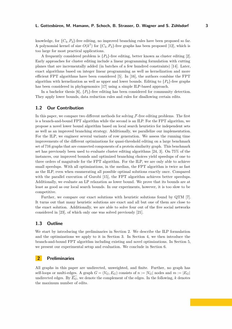
Figure 2 Number of permutations of graphs of the COG dataset that require at least 20 editsand can be solved within a certain total running time / with a certain number of recursive calls(and extra lower bound updates for -MP). The horizontal black line indicates the total number ofgraphs and node permutations that require 20 or more edits, including unsolved instances.

a sweet spot that gives the best overall running time. The basic greedy bounds need 10 to24 times as many calls as the other bounds in the median. The recomputed greedy bound -Gis slightly better than the updated one -U, -LP is the best, followed by -LS and -MD.

Nonetheless, for very small time limits, -U solves the highest number of instances. Forlarger time limits, reducing the number of calls pays off, though not at any cost. The medianspeedup of min-degree over the LP is 2.16 while needing 47% more calls in the median. Localsearch avoids their substantial memory overhead and spends significantly less time per callthan both. It needs 83% of the calls of -MD while being a factor of 12.36 faster in the median.It is never slower, and on 5% of the instances even more than 137 times faster than -MD.

Comparing the state-of-the-art FPT-MD-F-All algorithm to our FPT-LS-MP-All algorithm,we need 4.33 times less calls and are 46.06 times faster in the median. We are never slower,on 75% of the instances more than 16 times and on 5% of the instances more than 1044times faster. In conclusion, our local search lower bound gives high-quality bounds whilebeing fast. Our branching rules reduce the running time by another small factor while earlypruning mainly reduces the number of calls. Overall, we achieve a speedup of one to threeorders of magnitude over the state-of-the-art.

5.2 Parallelization

The left part of Figure 3 reports the speedup of FPT-LS-MP-All-MT over its sequentialcounterpart FPT-LS-MP-All, the sequentially fastest variant on the COG dataset. We showthe speedup with 1, 2, 4, 8 and 16 cores in comparison to the number of recursive calls andlower bound calculations. For each graph and permutation, we plot the speedup on thelast value of k for which the sequential version of the algorithm terminated within the timelimit. With only few recursive calls we cannot expect a good speedup. For a high number ofrecursive calls, FPT-LS-MP-All-MT achieves almost perfect speedup for all numbers of coreson many graphs. As the algorithm is executed with increasing values of k, for some graphsonly the last value of k needs a high number of calls and thus the overall speedup is notperfect even though in sum the number of calls is high.

10 Engineering Exact Quasi-Threshold Editing

101 102 103 104 105 106

Calls

0

2

4

6

8

10

12

14

16Sp

eedu

pFPT-LS-MP-All

Threads124816

10−2 10−1 100 101 102 103

Total Time [s]

0

500

1000

1500

2000

2500

Solve

d(G

raph

s×

Node

IdPe

rmut

atio

ns)

ILP-BILP-SILP-S-RILP-S-R-C4

Figure 3 Speedup of FPT-LS-M-All-MT and comparison of the different ILP variants on 16 (left)and 4 (right) node id permutations of the 716 COG graphs that require at least 20 edits.

10−2 10−1 100 101 102 103

Total Time [s]

0

500

1000

1500

2000

2500

Solve

d(G

raph

s×

Node

IdPe

rmut

atio

ns)

100 102 104 106

Calls

FPT-LS-MP-AllFPT-LS-MP-All-MTFPT-LS-MPFPT-LS-MP-MTILP-S-R-C4ILP-S-R-C4-MT

Figure 4 Comparison of the ILP to the FPT algorithm on 4 node id permutations of the 716COG graphs that require at least 20 edits.

5.3 Variants of the ILP

Figure 3 (right) shows the impact of the different optimizations on the ILP, when enabledone after another. We denote adding only one violated constraint by -S, adding constraintsduring relaxations by -R, and specialized C4 constraints by -C4. The baseline is ILP-B, whererow generation always adds all violated constraints for intermediate solutions.

In the median, ILP-S is just 5% faster than ILP-B. While on 95% of the instances it isat most 20% slower, it is more than 44 times faster on 5% of them, which explains the gapin Figure 3. ILP-S-R is not faster in the median, but on 95% of the instances at most 12%slower and on 5% it is at least 73% faster. The C4 constraints make the ILP 12% faster inthe median, at most 26% slower on 95% and at least 95% faster on 5% of the instances. Withall optimizations, the ILP solves 568 graphs. We also tried providing a heuristic solutionfrom QTM [7] to Gurobi, but the improvement was even smaller and disappeared in parallel.

Figure 4 compares the best ILP and FPT algorithms with and without -MT in terms ofrunning time and recursive calls. For the FPT algorithm, stopping at the first solution isnot slower on 95%, more than 52% faster on 50% and more than 3 times faster on 5% ofthe instances. Multi-threading incurs a measurable overhead. Compared to FPT-LS-MP-All,

L. Gottesbüren, M. Hamann, P. Schoch, B. Strasser, D. Wagner and S. Zühlsdorf 11

102 103

Actual k

1.00

1.05

1.10

1.15

1.20

1.25

1.30

QTM

k/

Actu

alk

Solved Graphs

103 104

Best Lower Bound

1.0

1.2

1.4

1.6

1.8

QTM

k/

Best

Lowe

rBou

nd

Unsolved Graphs

Figure 5 Comparison of heuristic solutions of QTM and the exact number of edits k for solvedgraphs (left) or the best lower bound for unsolved graphs (right) achieved by the FPT algorithm orthe ILP. For readability, we exclude one solved graph at k = 64, where QTM needed 202 edits.

FPT-LS-MP-All-MT is at most 16% slower on 95%, 78% faster in the median and more than12 times faster on 5% of the instances. When stopping at the first solution, this decreases to24% slower, 1% faster and 10 times faster, as more branches that do not lead to a solution areexplored in multi-threaded mode. FPT-LS-MP-MT is still 4% faster than FPT-LS-MP-All-MTin the median, at most 3% slower on 95% and at least 68% faster on 5% of the instances.

The parallel ILP is at most 5% slower on 95%, as fast in the median and more than 52%faster on 5% of the instances than the sequential ILP. Thus, the parallelization helps theFPT algorithm more than the ILP. A likely cause is that Gurobi needs much less searchnodes than the FPT algorithm which offer less potential for parallelism – on 50% of theinstances at least 185 times less, and on many graphs even just one or two, see Figure 4.

The speedup of FPT-LS-MP over ILP-S-R-C4 is at least 0.59 on 95%, 3.25 in the medianand at least 10.72 on 5% of the instances. For FPT-LS-MP-All, this decreases to 0.29, 2.10and 7.02. In parallel, the speedups are 1.09, 3.41 and 16.45 for all solutions, and 1.34, 3.67and 18.14 for the first solution. Single-threaded, the ILP solves more instances within 1000seconds than the FPT algorithm, indicating that for difficult instances better bounds aremore important. Overall, the FPT algorithm is often faster than the ILP, in particular inparallel and even when listing all solutions.

5.4 Comparison to QTMFigure 5 compares the results of the heuristic Quasi-Threshold Mover (QTM) [7] with exactresults for solved and the best lower bounds for unsolved graphs. We use the maximumvalue of k achieved for any permutation by FPT-LS-MP-MT and by ILP-S-R-C4 with andwithout -MT. If any of the algorithms solved the graph, we list it in the left part, otherwisein the right part. For QTM, we report the minimum k that QTM found over 16 runs. Again,the plot excludes 3248 graphs that require less than 20 edits. Of those, QTM solved 3172exactly, 56 with offset 1, 15 with offset 2 and 5 with offset 3. Of the remaining graphs, 588are solved and 128 are unsolved. Of the solved graphs, QTM solved 319 graphs exactly. Fornone of the unsolved graphs, QTM matches the lower bound. For 95% of the 716 graphs,QTM needs at most 1.22 times the edits of the exact solution or the lower bound.

12 Engineering Exact Quasi-Threshold Editing

Table 1 Overview of the social network graphs. Using the algorithms FPT-LS-MP and ILP-S-R-C4with 1 and 16 cores, we report the maximum k that finished within 1000 seconds, and the minimumtime over all permutations that is needed to find the first solution. In the case of football, wereport the time needed to show that there is no solution with that k.

FPT ILP1 core 16 cores 1 core 16 cores

Graph n m k Time [s] k Time [s] k Time [s] k Time [s]

karate 34 78 21 0.01 21 0.01 21 0.02 21 0.03lesmis 77 254 60 0.17 60 0.13 60 0.96 60 0.97grass_web 75 113 34 1.81 34 0.21 34 2.91 34 2.83dolphins 62 159 70 126.54 70 18.57 70 23.81 70 12.10

football 115 613 223 929.55 228 649.94 235 1000.01 237 1000.05

5.5 Social Network Instances

Table 1 shows an overview of the social networks with results for FPT-LS-MP and ILP-S-R-C4.Both solve karate and lesmis in less than a second, and grass_web within 3 seconds, withthe FPT algorithm being faster. Even though lesmis is both larger than grass_web andrequires 60 edits instead of 34, both algorithms are significantly slower on grass_web. Thisshows that their performance depends on the specific structure of the graph and not just thegraph size and k. For dolphins, the ILP is faster than the FPT algorithm. For all graphs,the FPT algorithm scales better with the number of cores. None of the algorithms can solvethe football network. We show that there is no solution for k ≤ 223, k ≤ 228 using theFPT algorithm with 1 or 16 cores respectively, and k ≤ 235, k ≤ 237 using the ILP with 1or 16 cores respectively. The previously best known upper bound was 251, computed withQTM [7] in 2.5ms. In 1000 seconds, the ILP shows a new upper bound of 250. For thesmallest three social networks, we verify that the best heuristic solutions in [7] are exact.QTM needs 72 edits on dolphins, whereas 70 edits are optimal. Appendix C contains adetailed analysis of the solution space with a focus on the community detection application.

6 Conclusion

We have introduced optimizations for two different approaches to solving any F-free edgeediting problem. We evaluate our optimizations for the special case of quasi-threshold editingon a set of 716 protein interaction graphs. For the first approach, the FPT algorithm, weshow that the combination of good lower bounds with careful selection of branches allows toreduce the running time by one to three orders of magnitude for 75% of the instances. Forthe second approach, an ILP, we evaluate several variants of row generation and show thatthey achieve small speedups. We show that the FPT algorithm is slightly faster than theILP, with a larger margin in parallel, and it can easily enumerate all optimal solutions. Forthe heuristic editing algorithm QTM, we show that on 95% of the instances, it needs at most22% more edits than our exact solutions or lower bounds indicate.

Comparing the structure of exact vs. heuristic solutions might give further insights howto improve heuristics. Exact FPT algorithms could be further improved by better bounds,possibly based on LP relaxations. As the COG benchmark set actually contains edit costs,an extension of our optimizations to the weighted editing problem could be investigated.

L. Gottesbüren, M. Hamann, P. Schoch, B. Strasser, D. Wagner and S. Zühlsdorf 13

References1 Diogo V. Andrade, Mauricio G. C. Resende, and Renato F. Werneck. Fast local search

for the maximum independent set problem. Journal of Heuristics, 18(4):525–547, 2012.doi:10.1007/s10732-012-9196-4.

2 Sebastian Böcker and Jan Baumbach. Cluster Editing. In Proceedings of the 9th Conferenceon Computability in Europe (CiE’13), volume 7921 of Lecture Notes in Computer Science,pages 33–44. Springer, 2013. doi:10.1007/978-3-642-39053-1_5.

3 Sebastian Böcker, Sebastian Briesemeister, Quang Bao Anh Bui, and Anke Truß. A fixed-parameter approach for Weighted Cluster Editing. In Proceedings of the 6th Asia-PacificBioinformatics Conference (APBC 2008), volume 6, pages 211–220, 2008. doi:10.1142/9781848161092_0023.

4 Sebastian Böcker, Sebastian Briesemeister, Quang Bao Anh Bui, and Anke Truß. Goingweighted: Parameterized algorithms for cluster editing. Theoretical Computer Science,410(52):5467–5480, December 2009. doi:10.1016/j.tcs.2009.05.006.

5 Sebastian Böcker, Sebastian Briesemeister, and Gunnar W. Klau. Exact Algorithms forCluster Editing: Evaluation and Experiments. Algorithmica, 60(2):316–334, 2011. doi:10.1007/s00453-009-9339-7.

6 Felix Bohlmann. Graphclustern durch Zerstören langer induzierter Pfade. Bachelorthesis, TU Berlin, 2015. URL: http://fpt.akt.tu-berlin.de/publications/theses/BA-felix-bohlmann.pdf.

7 Ulrik Brandes, Michael Hamann, Ben Strasser, and Dorothea Wagner. Fast Quasi-ThresholdEditing. In Proceedings of the 23rd Annual European Symposium on Algorithms (ESA’15),volume 9294 of Lecture Notes in Computer Science, pages 251–262. Springer, 2015. doi:10.1007/978-3-662-48350-3_22.

8 Leizhen Cai. Fixed-parameter tractability of graph modification problems for hereditary prop-erties. Information Processing Letters, 58(4):171–176, May 1996. doi:10.1016/0020-0190(96)00050-6.

9 Frank Pok Man Chu. A simple linear time certifying LBFS-based algorithm for recognizingtrivially perfect graphs and their complements. Information Processing Letters, 107(1):7–12,June 2008. doi:10.1016/j.ipl.2007.12.009.

10 Peter Damaschke. Fixed-Parameter Enumerability of Cluster Editing and Related Problems.Theory of Computing Systems, 46(2):261–283, 2008. doi:10.1007/s00224-008-9130-1.

11 Hassan Ali Dawah, Bradford A. Hawkins, and Michael F. Claridge. Structure of the ParasitoidCommunities of Grass-Feeding Chalcid Wasps. Journal of Animal Ecology, 64(6):708–720,1995. doi:10.2307/5850.

12 Pål Grønås Drange and Michał Pilipczuk. A Polynomial Kernel for Trivially Perfect Editing.Algorithmica, 80(12):3481–3524, December 2017. doi:10.1007/s00453-017-0401-6.

13 Michelle Girvan and Mark E. J. Newman. Community structure in social and biologicalnetworks. Proceedings of the National Academy of Science of the United States of America,99(12):7821–7826, 2002. doi:10.1073/pnas.122653799.

14 Martin Grötschel and Yoshiko Wakabayashi. A cutting plane algorithm for a clusteringproblem. Mathematical Programming, 45(1-3):59–96, 1989. doi:10.1007/BF01589097.

15 Gurobi Optimization, LLC. Gurobi optimizer reference manual, 2020. URL: http://www.gurobi.com.

16 Sepp Hartung and Holger H. Hoos. Programming by Optimisation Meets ParameterisedAlgorithmics: A Case Study for Cluster Editing. In Proceedings of the 9th InternationalConference on Learning and Intelligent Optimization, Lecture Notes in Computer Science,pages 43–58. Springer, 2015. doi:10.1007/978-3-319-19084-6_5.

17 Marc Hellmuth, Nicolas Wieseke, Marcus Lechner, Hans-Peter Lenhof, Martin Middendorf, andPeter F. Stadler. Phylogenomics with paralogs. Proceedings of the National Academy of Scienceof the United States of America, 112(7):2058–2063, 2015. doi:10.1073/pnas.1412770112.

14 Engineering Exact Quasi-Threshold Editing

18 Donald E. Knuth. The Stanford GraphBase : a platform for combinatorial computing. Addison-Wesley, 1993.

19 Yunlong Liu, Jianxin Wang, Jie You, Jianer Chen, and Yixin Cao. Edge deletion problems:Branching facilitated by modular decomposition. Theoretical Computer Science, 573:63–70,2015. doi:10.1016/j.tcs.2015.01.049.

20 David Lusseau, Karsten Schneider, Oliver Boisseau, Patti Haase, Elisabeth Slooten, and SteveDawson. The Bottlenose Dolphin Community of Doubtful Sound Features a Large Proportionof Long-Lasting Associations. Behavioral Ecology and Sociobiology, 54(4):396–405, September2004. doi:10.1007/s00265-003-0651-y.

21 James Nastos. Utilizing graph classes for community detection in social and complex networks.PhD thesis, University of British Columbia, 2015. doi:10.14288/1.0074429.

22 James Nastos and Yong Gao. A Novel Branching Strategy for Parameterized Graph Modi-fication Problems. In Proceedings of the 4th International Conference on CombinatorialOptimization and Applications, volume 2 of Lecture Notes in Computer Science, pages 332–346.Springer, 2010. doi:10.1007/978-3-642-17461-2_27.

23 James Nastos and Yong Gao. Familial groups in social networks. Social Networks, 35(3):439–450, July 2013. doi:10.1016/j.socnet.2013.05.001.

24 Sven Rahmann, Tobias Wittkop, Jan Baumbach, Marcel Martin, Anke Truß, and SebastianBöcker. Exact and Heuristic Algorithms for Weighted Cluster Editing. In Proceedings of the6th Annual International Conference on Computational Systems Bioinformatics (CSB 2007),volume 6, pages 391–401, 2007. doi:10.1142/9781860948732_0040.

25 Christian Staudt, Aleksejs Sazonovs, and Henning Meyerhenke. NetworKit: A tool suitefor large-scale complex network analysis. Network Science, 4(4):508–530, December 2016.doi:10.1017/nws.2016.20.

26 Wayne W. Zachary. An Information Flow Model for Conflict and Fission in Small Groups.Journal of Anthropological Research, 33:452–473, 1977. doi:10.1086/jar.33.4.3629752.

L. Gottesbüren, M. Hamann, P. Schoch, B. Strasser, D. Wagner and S. Zühlsdorf 15

A B C

B C

BC

A C

AC

A B

CB

Figure 6 Example Recursion Tree. Children are explored from left to right. The “No Redundancy”optimization prunes the red part.

A Avoiding Redundancy

Our algorithm maintains a global symmetric n × n-bit matrix. The entries in the matrixcorrespond to node pairs. If a bit is set, the corresponding node pair must not be editedanymore. We refer to these node pairs as blocked. In the following, we describe in detail howthese optimizations that were introduced in [10] work.

A.1 No UndoEvery solution that edits a node pair twice can be improved by not editing the node pair atall. We exploit this observation by setting the bit corresponding to the performed edit whenrecursing. When ascending from the recursion, we reset the bit. The same optimization hasalso been used in [6] and is the basis of efficient branching rules for cluster editing [4].

A.2 No RedundancyA possible recursion tree is depicted in Figure 6. Note how multiple branches contain thesame set of edits, but the edits appear in a different order.

We ensure that every branch enumerates a different set of edits, by unblocking a node paironly after all sibling edits have been explored. In particular, this ensures that every solutionis enumerated exactly once. Consider the first recursion level of the example in Figure 6.The edits are explored in the following order: A, then B, and finally C. Before descendinginto the branch of A, we set A’s bit. After ascending from A’s branch and reverting thecorresponding edit, the corresponding bit is not reset. In addition to A’s bit, we set B’s bitand descend into B’s branch. Finally, we ascend from B’s branch, leave its bit set, set C’sbit and descend into C’s branch. After all edits in a recursion level are explored, all bits setin this level are reset, i.e., we reset A’s, B’s and C’s bit.

B Implementation Details

In this section, we document various details of our implementation. We first describe ourgraph data structure and how we iterate over it. In Section B.1, we describe how we listforbidden subgraphs. We maintain subgraph counters that we describe in Section B.2. InSection B.3, we describe for each lower bound algorithm how it is implemented using theaforementioned subgraph listing algorithms. In Section B.4, we describe the implementationof our branching strategy. Finally, in Section B.5, we describe our parallelization in detail.

We store our graph as an adjacency matrix with 1 bit per node pair. To enumerateedges or neighbors, we use special CPU instructions to count leading zeros in a copy of a 64bit block of this matrix. We then remove the found 1-bit from the 64 bit block and countagain. If the current 64 bit block contains only zeros, we move to the next one. All but thelargest 24 graphs in our benchmark set have at most 320 nodes, thus requiring at most five

16 Engineering Exact Quasi-Threshold Editing

64 bit blocks per row of the matrix. The largest graph has 8836 nodes and thus requires 13964 bit blocks per row, but its average degree is also 64, therefore on average almost everysecond block contains a 1-bit. Thus, for almost all of the graphs we consider, bit matricesseem an appropriate choice in terms of memory usage and enumeration efficiency. For thelarger graphs, adjacency arrays might be a better choice but as we are far from solving them,we did not further explore this. Adjacency matrices have the advantage that we can easilycombine multiple rows to list common neighbors or exclude neighbors of another node, afeature that we use for subgraph listing as described in the following. Let A[i, j] denote theentry of the adjacency matrix in row i and column j. We use matrix slice notation A[:, j] todenote column j, and A[i, :] to denote row i, i.e., the neighbors of node i.

B.1 Subgraph ListingTo select subgraphs for branching and calculating lower bounds, we need to enumerate allforbidden subgraphs. In preliminary experiments, we found that enumerating forbiddensubgraphs on demand does not only require much less memory than storing them, but is alsomuch faster. Our implementation provides two methods for this: a global one that lists allforbidden subgraphs and a local one that lists all subgraphs containing a certain node pair.The latter is required to efficiently implement our local search lower bound and the branchingon most useful node pairs. For simplicity, our descriptions focus on {C4, P4}-listing but oursource code works for arbitrary {Cl, Pl}, l ≥ 4 and {Pl}, l ≥ 2.

Global Listing. For the listing of all forbidden subgraphs, we enumerate all edges. Weconsider each edge {u2, u3} as the central edge and then enumerate edges {u1, u2} in theouter loop, and {u3, u4} in the inner loop, to complete the P4 or C4. For listing candidatesu1, we directly exclude neighbors of u3 by only iterating over A[u1, :] ∧ (¬A[u3, :]). We listcandidates u4 analogously. Fixing the central edge ensures each induced P4 is listed exactlyonce. We list each C4 four times, which we use for trying different shareable node pairs forthe packing lower bounds, as each edge deletion transforms the C4 into a P4.

Local Listing. For the listing of forbidden subgraphs that contain a certain node pair {u, v},we need to consider all positions of {u, v} in the forbidden subgraph. If {u, v} is an edge, thismeans that apart from the case where {u, v} is the central edge, we also need to consider thecase where we extend the path twice on each side. If {u, v} is not an edge, the case where{u, v} consists of the two degree-1-nodes of the P4 can be omitted due to the optimizationsdiscussed in Section 4.2. We only need to find common neighbors x ∈ A[u, :] ∧ A[v, :] of uand v. These are part of the central edge. We try extending the path by one edge from u

and v separately, i.e., iterate over A[u, :] ∧ (¬A[x, :]) and A[v, :] ∧ (¬A[x, :]).

Listing For Lower Bounds. For lower bounds, we are only interested in forbidden subgraphsthat do not contain any node pair that is already used in the lower bound. We maintaina bit matrix L where all node pairs that are already used in the bound are set to 1. Byusing A[u, :] ∧ (¬L[u, :]) instead of A[u, :] for neighbors of u and (¬A[u, :]) ∧ (¬L[u, :]) fornon-neighbors, we can directly exclude these node pairs from listing.

Excluding Specific Node Pairs From Listing. To branch on its node pairs or to check if asubgraph can be added to a lower bound, we need to enumerate its node pairs. For this, weimplicitly exclude blocked node pairs as well as {u1, u4}, which is the node pair of degree

L. Gottesbüren, M. Hamann, P. Schoch, B. Strasser, D. Wagner and S. Zühlsdorf 17

one in a P4. As mentioned before, we always list a C4 four times, and thus omit a differentedge {u1, u4} in each enumeration. This lets the lower bound algorithms select the best nodepair to share or the branching strategy select the best node pair to exclude.

B.2 Subgraph CountersIn our Most and Most Pruned branching strategies and the local search lower bound, we wantto select the subgraph whose node pairs cover the most or least other forbidden subgraphs.For this, we maintain a counter for each node pair in how many forbidden subgraphs it iscontained. Whenever a node pair is edited or blocked/unblocked we update the counters.When blocking a node pair, we store its previous counter on a stack so that it can be easilyrestored when unblocking, and set the current counter to zero. Note that our counters counta C4 three times for edges and four times for non-edges due to listing the C4 four times andomitting one of the edges each time. We also maintain the sum of the subgraph counters tobe able to quickly check if there are any forbidden subgraphs at all.

B.3 Lower Bound AlgorithmsEach of our lower bound algorithms has both a thread-state that is maintained once perthread and a call-state that is copied for every recursive call. We compute an initial lowerbound on the input graph and start our search for kopt from this bound instead of 0. Thecall-state is initialized once during this initial lower bound calculation and then used asinitialization for all ks that we try. For most algorithms, the call-state contains the previouslycalculated lower bound as an array of subgraphs (node tuples) in the packing. We passthe call-state down into recursive calls, but not back up. The rationale behind this is thatwe need to remove at most one forbidden subgraph from the bound when descending intorecursion, whereas no longer blocked node pairs would force a lot of subgraphs to be removedwhen returning from a recursive call.

Basic Bound. For the basic bound, we globally enumerate forbidden subgraphs H andadd H to the packing P if none of its node pairs are used by another graph in the packing.This is done in each recursive call with an initially empty packing. After the one pass, P isinclusion-maximal. We maintain a bit matrix C for node pairs covered by the packing in thethread-state. When adding H to P , we mark its node pairs in C. We also supply a referenceof C to the listing algorithm to skip subgraphs we cannot use. As additional bits in C areset during the listing, it does not skip all subgraphs we cannot use. For example, the listingdoes not check the central node pair again. In preliminary experiments this still gave a smallspeedup.

Updates. For the basic bound with updates we pass the packing P through the search tree.Before descending into recursion, we remove the subgraph H that contains the edited nodepair {u, v} from P , if it exists. If possible, we add subgraphs H ′ to P that share a node pairwith H or contain {u, v}, to make P inclusion-maximal. This is done using the local listing.Similar to before, the local listing skips some subgraphs touched by C. We store a list ofsubgraphs in the packing in the call-state. For memory efficiency, we do not store C in thecall-state but instead recompute it from scratch when modifying the bound.

Local Search. The local search lower bound also just maintains the list of subgraphs usedin the bound in its call-state. The initial update works as described above. To find candidates

18 Engineering Exact Quasi-Threshold Editing

for replacing one subgraph by one or more subgraphs, we use the local listing. In each round,we try to replace each subgraph H in the packing once. For this, we first remove H from P

and then use the local listing on all node pairs of H to obtain the set R of subgraphs thatcould replace H. From R, we obtain candidates that can be inserted together. For eachsubgraph H ′ ∈ R we first insert it into P , and then iterate over the rest of R, trying to insert.If at least one additional candidate was found, we keep them in the packing. Otherwise, wecan only replace H by H ′. With 70% probability we take the H ′ that covers the fewest otherforbidden subgraphs, and with 30% probability we choose a random one from R.

We apply several optimizations to speed up the search for additional candidates. Foreach node pair of H, we store a separate list of candidates. This allows us to skip candidatesthat use a node pair that is used by an already included candidate, without considering eachcandidate separately. To avoid trying the same candidate twice, we also list candidates onlyfor the first node pair they contain by excluding the already considered node pairs from thecandidate search for subsequent node pairs.

Min-Degree Heuristic. The min-degree heuristic is based on the independent set formula-tion where a subgraph is a node and two nodes are connected by an edge if the correspondingsubgraphs share a node pair. A good lower bound then corresponds to a large independentset. For independent sets, the min-degree heuristic iteratively adds the node with the smallestremaining degree to the independent set and then deletes it and its neighbors from the graph.Instead of explicitly constructing this graph model, we translate this formulation back toforbidden subgraphs.

We iteratively add subgraphs to the bound whose node pairs are shared with the leastnumber of subgraphs that can still be added to the bound. To implement it, we need toexplicitly maintain the “degree” of every subgraph in a priority queue as it is changing overtime as more and more subgraphs are added to the bound. For this, we (temporarily) storean explicit list of all forbidden subgraphs that we obtain through global listing. Further,for every node pair we store a list of subgraphs it is part of by storing their indices in thelist of subgraphs. Similarly, we store these list indices in the priority queue. This allowsto efficiently identify the elements that need to be updated or removed from the priorityqueue. For a subgraph H, we initially use the sum over all node pairs of H of the number ofsubgraphs that contain the node pair as key. This might count the same subgraph severaltimes, but is more efficient to calculate. Preliminary experiments showed that this is fasterthan calculating the actual number of subgraphs with whom H shares a node pair.

Whenever we take a subgraph H from the priority queue and add it to the bound, weneed to remove its neighbors from the priority queue and update their neighbors’ degreesaccordingly. To obtain the neighbors N of H, we iterate over H’s node pairs and list allsubgraphs they are part of. We remove each subgraph n ∈ N from the priority queue andfor each of n’s neighbors, we decrement its key in the priority queue by one.

For the priority queue, we use a bucket priority queue. As nodes only need to be movedbetween adjacent buckets, we can maintain all buckets in one large array and move elementsbetween buckets by swapping them to the boundary and then adjusting the boundary.

LP Relaxation. The LP for our LP bound corresponds exactly to the ILP formulation shownin Section 3 with the optimization of omitting one node pair as described in Section 3.2.Our main goal for the implementation of the LP bound was to have a comparison with alower bound algorithm that is guaranteed to prune at least as good as the packing-basedlower bounds. For this reason, we ensure that the LP always contains the constraints that

L. Gottesbüren, M. Hamann, P. Schoch, B. Strasser, D. Wagner and S. Zühlsdorf 19

correspond to forbidden subgraphs that could also be used in the packing-based lower bound.Similar to the ILP, we initialize the LP with all constraints that correspond to forbiddensubgraphs in the input graph. Whenever we edit or block a node pair, we fix the value of itscorresponding value to 1 or 0, depending on whether it is now connected by an edge or not.When a node pair is edited, it is always blocked and thus all constraints that correspond toforbidden subgraphs that no longer exist in the edited graph are trivially fulfilled and there isthus no need to remove them explicitly. After each edit, we add constraints that correspondto forbidden subgraphs that contain the edited node pair. After undoing an edit, we removethem again, as the LP solver slows down when the LP contains a lot of constraints.

B.4 Branching StrategiesAs described in Section 4.5, we want to prefer subgraphs that contain at most one non-blockednode pair, as we know this edit has to be applied. In a call-state like those of the lowerbound algorithms, we store both this list of subgraphs, and a flag indicating whether thebranch can be pruned. Such subgraph can only appear when blocking or editing a nodepair {u, v}. Every time this happens, we enumerate all subgraphs H containing {u, v}. If Hcontains exactly one non-blocked node pair, we store it. If H contains only blocked nodepairs, the current branch can be pruned immediately because H cannot be destroyed. Beforethe branching strategy selects a forbidden subgraph, we first check if the flag is set and returnan empty list of node pairs, if so. Otherwise, we iterate over the list of subgraphs in thecall-state and return the only non-blocked node pair of the first subgraph of the list wherethis node pair has not been edited yet. Note that two of these subgraphs might containthe same non-blocked node pair, thus after the first of them has been selected, the secondbecomes invalid.

Only if the flag is not set and there is no subgraph with exactly one non-blocked node pair,we apply the actual branching strategy. In our Most and Most Pruned branching strategies,we avoid listing all forbidden subgraphs. Instead, we first identify those node pairs thatare part of the maximum number of subgraphs using the subgraph counters introduced inSection B.2. Due to our lexicographical ordering, we are only interested in those subgraphsthat contain these node pairs. We use our local listing to enumerate them and select themaximum as described in Section 4.5. The output of the branching strategy is a sorted list ofnode pairs and a flag whether the graph is solved. We set this flag if the sum of the subgraphcounters is zero.

B.5 ParallelizationIn our parallelization, different threads explore different branches of the search tree. Wemaintain a global queue of work packages that represent roots of unexplored branches. Toachieve a scalable parallelization we want to generate few work packages that have a lot ofrecursive calls left. Due to our optimizations, we cannot know in advance how many callsare left for a certain branch. Even branches that start at the root of our recursion tree mightbe pruned after a single call. Therefore, we need to generate work packages as we explorethe search tree, i.e., employ work-stealing.

Each work package contains the number of remaining edits, the graph, the blocked nodepairs, the subgraph counters and the call-states of the lower bound and the branching strategy(can be empty). Hence, creating a work package for every call is too expensive, as we wouldneed to copy these data structures, whose memory consumption is quadratic in the numberof nodes. Passing them through the search tree, and updating on-the-fly is fast, but a work

20 Engineering Exact Quasi-Threshold Editing

package constitutes the root of a new search tree and thus requires a copy. Therefore, weonly create work packages when the global work queue contains less work packages than thenumber of threads.

When a worker finishes one recursion tree, it takes another work package from the queue.If there is none left, it waits until either work becomes available or the algorithm is finished.The latter is indicated either by the fact that no thread has a work package anymore (wekeep a counter how many threads are currently working), or a global flag that is set when thefirst solution has been found and not all solutions shall be listed. This flag is also checked ineach recursive call to ensure that if one thread finds a solution, all other threads terminate.

At the beginning of every recursive call, we check if work packages shall be generated. Asimple approach would be to split the recursive calls of the current search tree node intowork packages. Unfortunately, this does not scale well, as we would predominantly creatework packages on deeper recursion levels where only few edits remain. Instead, we split offunexplored branches from the top of the current recursion tree, where we hope the most workis left. For this, we explicitly maintain the current recursion path of each worker thread.

Each element of the path contains the node pairs to branch on, the call-states of thebound and the branching strategy for each of these branches and an index that indicates thenext branch to be explored. After potentially generating work packages, we invoke the lowerbound calculation. We then check if the recursive call can be pruned because of the bound,because there are no more edits left or because a solution has been found. If not, we createits element in the path. For this, we obtain the node pairs for the next recursion level fromthe branching strategy. We then create copies of the call-states for all of them and updatethem such that each of them can be directly used to create a work package. This ensuresthat work package generation, which happens inside a global lock, is quick and does not needto update call-states. For the early pruning (see Section 4.6), we also directly check if callscan be pruned and if yes, we directly remove them from the node pairs.

For the actual recursive calls, we iterate over the node pairs in the element of the path.We advance the index that indicates the next call and execute an actual recursive call withthe call-state for that node pair. After all recursive calls finished, we remove the elementfrom the path. It is possible that during a recursive call on a lower level work packages havebeen generated for the remaining node pairs. In this case, the path will be empty when therecursive call returns. We check for this, and then return directly instead of continuing withthe remaining node pairs.

For our recursive calls, we also update a copy of the graph, the blocked node pairs andthe subgraph counters that are used for calculating lower bounds and the branching strategy.Additionally to this copy that represents the state at the bottom of our path, we also maintaina copy that corresponds to the state at the top of the path that is used for generating workpackages.

To generate work packages, we first advance the top state to the next node pair thathas not been used for a recursive call. For all remaining node pairs of the top element ofthe path we generate a separate work package using the top state and the call-state that isstored in the path’s element. Then, we remove the top of the path. This continues with thenew top of the path, until either the recursion path is empty or a sufficient number of workpackages (2x number of threads) are in the queue.

Note that we generate work packages before creating the element in the path thatcorresponds to the current recursive call. Hence, the generating thread still has work left,even if the recursion path becomes empty. This is to avoid that a thread immediately needsto get another work package after putting work into the global queue.

L. Gottesbüren, M. Hamann, P. Schoch, B. Strasser, D. Wagner and S. Zühlsdorf 21

100 101 102 103

k

100

101

102

103

104

105

106

107Nu

mbe

rofS

olut

ions

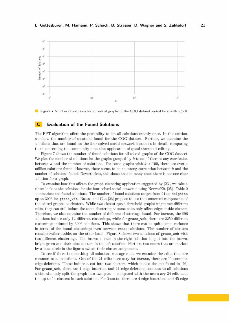
Figure 7 Number of solutions for all solved graphs of the COG dataset sorted by k with k > 0.

C Evaluation of the Found Solutions

The FPT algorithm offers the possibility to list all solutions exactly once. In this section,we show the number of solutions found for the COG dataset. Further, we examine thesolutions that are found on the four solved social network instances in detail, comparingthem concerning the community detection application of quasi-threshold editing.

Figure 7 shows the number of found solutions for all solved graphs of the COG dataset.We plot the number of solutions for the graphs grouped by k to see if there is any correlationbetween k and the number of solutions. For some graphs with k > 100, there are over amillion solutions found. However, there seems to be no strong correlation between k and thenumber of solutions found. Nevertheless, this shows that in many cases there is not one clearsolution for a graph.

To examine how this affects the graph clustering application suggested by [23], we take acloser look at the solutions for the four solved social networks using NetworKit [25]. Table 2summarizes the found solutions. The number of found solutions ranges from 24 on dolphinsup to 3006 for grass_web. Nastos and Gao [23] propose to use the connected components ofthe edited graphs as clusters. While two closest quasi-threshold graphs might use differentedits, they can still induce the same clustering as some edits only affect edges inside clusters.Therefore, we also examine the number of different clusterings found. For karate, the 896solutions induce only 12 different clusterings, while for grass_web, there are 2250 differentclusterings induced by 3006 solutions. This shows that there can be quite some variancein terms of the found clusterings even between exact solutions. The number of clustersremains rather stable, on the other hand. Figure 8 shows two solutions of grass_web withtwo different clusterings. The brown cluster in the right solution is split into the brown,bright-green and dark-blue clusters in the left solution. Further, two nodes that are markedby a blue circle in the figures switch their cluster assignment.

To see if there is something all solutions can agree on, we examine the edits that arecommon to all solutions. Out of the 21 edits necessary for karate, there are 11 commonedge deletions. These induce a cut into two clusters, which is also the cut found in [26].For grass_web, there are 1 edge insertion and 11 edge deletions common to all solutionswhich also only split the graph into two parts – compared with the necessary 34 edits andthe up to 14 clusters in each solution. For lesmis, there are 4 edge insertions and 45 edge

22 Engineering Exact Quasi-Threshold Editing

Table 2 Summary of the solutions found. For each graph, we report the number of differentsolutions, the number of different induced clusterings, the minimum and maximum number ofclusters in the different solutions, the number of insertions and deletions common to all solutions,the number of clusters obtained when just applying the common edits, the total number of differentinsertions and deletions and the number of clusters obtained when intersecting all found clusterings.

#Solu- #Clus- #Clusters Common UnionGraph k tions terings Min Max Ins. Del. Clus. Ins. Del. Clust.

karate 21 896 12 2 4 0 11 2 13 27 7grass_web 34 3006 2250 11 14 1 11 2 11 45 22lesmis 60 384 192 8 12 4 45 6 10 63 16dolphins 70 24 8 12 13 5 56 9 11 71 16

Figure 8 Two solutions of grass_web. Red edges have been deleted, green edges have beeninserted. Nodes are colored by connected component in the edited graph. The two blue circlesdenote two nodes that changed clusters.

deletions common to all solution which induce 6 clusters – this shows a structure that is alot more stable. On dolphins, there are 5 edge insertions and 56 edge deletions commonto all solutions, i.e., each solution only adds 9 further edits. These common edits alreadyinduce 9 clusters which is close to the 12 or 13 clusters found in the individual solutions.

Additionally, we look at the number of edits in the union of solutions. For all graphs thereare more edge deletions than insertions. Even if all edge insertions were in a single solution,in all graphs but karate there were more than two times more edge deletions than insertions.Further, we calculate the intersection of all found clusterings to obtain the largest clustersthat are not split in any solution. For karate, this gives us 7 clusters that split both of thetwo parts into further parts. For grass_web, we even obtain 22 clusters (compared with atmaximum 14 clusters in an individual solution). For lesmis and dolphins, we obtain 16clusters, i.e., a value relatively close to the up to 12 or 13 clusters that are found in individualsolutions.

This analysis shows the power of being able to enumerate all solutions. We can not onlydetermine how stable the clustering structure of a graph is, we can also obtain smallestcomponents on which all different solutions agree – or large clusters, where all solutions agreethat they should be split. This could also be used to obtain overlapping clusters by assigningnodes that frequently change between clusters to several clusters.