Journal of Biomolecular NMR 29: 223–242, 2004.© 2004 Kluwer Academic Publishers. Printed in the Netherlands.

223

Exact solutions for internuclear vectors and backbone dihedral anglesfrom NH residual dipolar couplings in two media, and their application ina systematic search algorithm for determining protein backbone structure

Lincong Wanga & Bruce Randall Donalda,b,c,∗,∗∗aDartmouth Computer Science Department, bDartmouth Chemistry Department, and cDartmouth Department ofBiological Sciences, Hanover, NH 03755, U.S.A.

Received 26 June 2003; Accepted 11 February 2004

Key words: algorithms for protein structure determination, conformational search, exact solutions for backbonedihedral angles, exact solutions for internuclear vectors, global fold determination, high-throughput NMR methods,protein kinematics, residual dipolar couplings, structural genomics, systematic search

Abstract

We have derived a quartic equation for computing the direction of an internuclear vector from residual dipolarcouplings (RDCs) measured in two aligning media, and two simple trigonometric equations for computing thebackbone (φ,ψ) angles from two backbone vectors in consecutive peptide planes. These equations make it possibleto compute, exactly and in constant time, the backbone (φ,ψ) angles for a residue from RDCs in two media on anysingle backbone vector type. Building upon these exact solutions we have designed a novel algorithm for determ-ining a protein backbone substructure consisting of α-helices and β-sheets. Our algorithm employs a systematicsearch technique to refine the conformation of both α-helices and β-sheets and to determine their orientations usingexclusively the angular restraints from RDCs. The algorithm computes the backbone substructure employing verysparse distance restraints between pairs of α-helices and β-sheets refined by the systematic search. The algorithmhas been demonstrated on the protein human ubiquitin using only backbone NH RDCs, plus twelve hydrogen bondsand four NOE distance restraints. Further, our results show that both the global orientations and the conformationsof α-helices and β-strands can be determined with high accuracy using only two RDCs per residue. The algorithmrequires, as its input, backbone resonance assignments, the identification of α-helices and β-sheets as well as sparseNOE distance and hydrogen bond restraints.

Abbreviations: NMR – nuclear magnetic resonance; RDC – residual dipolar coupling; NOE – nuclear Overhausereffect; SVD – singular value decomposition; DFS – depth-first search; RMSD – root mean square deviation; POF– principal order frame; PDB – protein data bank; SA – simulated annealing; MD – molecular dynamics.

Introduction

The increasing gap between the speeds of DNA se-quencing and protein structure determination requires

∗To whom correspondence should be addressed: 6211 SudikoffLaboratory, Dartmouth Computer Science Department, Hanover,NH 03755, U.S.A. E-mail: brd@cs.dartmouth.edu∗∗This work is supported by the following grants to B.R.D.:National Institutes of Health (R01 GM 65982), National Sci-ence Foundation (IIS-9906790, EIA-0102710, EIA-0102712, EIA-9818299, EIA-0305444 and EIA-9802068), and the John SimonGuggenheim Foundation.

the development of efficient algorithms to computestructures as accurately as possible using only a min-imum number of restraints obtainable rapidly by ex-perimental techniques. One way to achieve this is todevelop algorithms whose key components are ana-lytic expressions computable in constant time.1 Herewe present such an algorithm for determining a pro-tein backbone structure using global angular (orienta-tional) restraints on internuclear vectors derived frombackbone residual dipolar couplings (RDCs) meas-ured in two aligning media (Tjandra and Bax, 1997;

224

Tolman et al., 1995). The RDCs can be recorded andassigned much faster than nuclear Overhauser effects(NOEs) required by traditional NMR structure determ-ination methods. Months of time can be required toassign a sufficient number of NOEs, especially thoseinvolving sidechain protons, to compute an accurateNMR structure. Therefore, RDCs are better suitedfor developing high-throughput structure determina-tion methods. For example, algorithms have beendesigned to compute a protein fold with RDCs alone orwith RDCs plus other restraints such as chemical shiftsor sparse NOEs (Andrec et al., 2001; Delaglio et al.,2000; Fowler et al., 2000; Giesen et al., 2003; Huset al., 2001; Rohl and Baker, 2002; Tian et al.,2001). These methods require several sets of RDCsin one or two media and use a fragment replacementmethod (Andrec et al., 2001; Delaglio et al., 2000;Rohl and Baker, 2002), rely on heuristic algorithmsand molecular dynamics (Clore et al., 1999; Giesenet al., 2003; Hus et al., 2001), or employ RDCsonly for orienting ideal helices (Fowler et al., 2000).The fragment replacement method relies heavily onstatistics from the Protein Databank (PDB) (Bermanet al., 2000). A different search technique, systematicsearch, has been used successfully to determine thestructure of a tripeptide by solid-state NMR (Rienstraet al., 2002). A systematic search is a search overall possible conformations (solutions) that employsa provable pruning strategy that guarantees prunedconformations need not be considered further. In thispaper we demonstrate that by combining systematicsearch with exact solutions for computing, first, thedirections of an NH vector, then, (φ,ψ) angles in con-stant time for a single residue, it is possible to computea backbone substructure consisting of α-helices andβ-sheets using only RDCs in two media on a singlebackbone vector type plus very sparse distance re-straints. Further, our algorithm uses only the averagesfor the backbone (φ,ψ) angles from the PDB and doesnot rely on molecular dynamics.

Theoretical background

In this section we outline the derivation of a quarticequation used to compute the orientation of an in-ternuclear unit vector from RDCs in two media, andtwo simple trigonometric equations used to computethe backbone (φ,ψ) angles of residue i given oneunit vector in peptide plane i and another unit vec-tor in plane i + 1. These unit vectors are computed

from the quartic equation. Interested readers can referto Appendices A, B for the full details of derivationof the quartic and trigonometric equations. Then, wedescribe a recursive strategy for computing, con-secutively, the (φ,ψ) angles of all the residues of astructural fragment.

Computation of vector orientations

The equations for NH RDCs measured in two mediacan be written as (Saupe, 1968):

DNH

= Dmax(Sxxx2 + Syyy2 + Szzz

2), (1)

D′NH

= Dmax(S′xxx ′2 + S′

yyy′2 + S′

zzz′2), (2)

where Dmax is the dipolar interaction constant, DNH

,an NH RDC value in medium 1, Sxx, Syy and Szz thethree diagonal elements of a diagonalized Saupe mat-rix S (the alignment tensor) for medium 1. A Saupematrix (a 3 × 3 traceless and symmetric matrix) spe-cifies the ensemble-averaged anisotropic orientation ofa molecule in the laboratory frame. x, y and z are, re-spectively, the x, y, z−components of an internuclearNH unit vector v = (x, y, z) in a principal order frame(POF) which diagonalizes S. D′

NHand S′

xx, S′yy , S′

zz ofS′ are the corresponding variables for medium 2 andv′ = (x ′, y ′, z′) is the same NH unit vector in a POFfor medium 2. v and v′ are related by

v′ = R12v, (3)

where R12 is a relative rotation matrix between the twoPOFs of medium 1 and 2. From Equations (1–3) wehave derived a quartic equation satisfied by x2:

f4u4 + f3u

3 + f2u2 + f1u + f0 = 0, (4)

u = 1 − 2(x

a

)2,

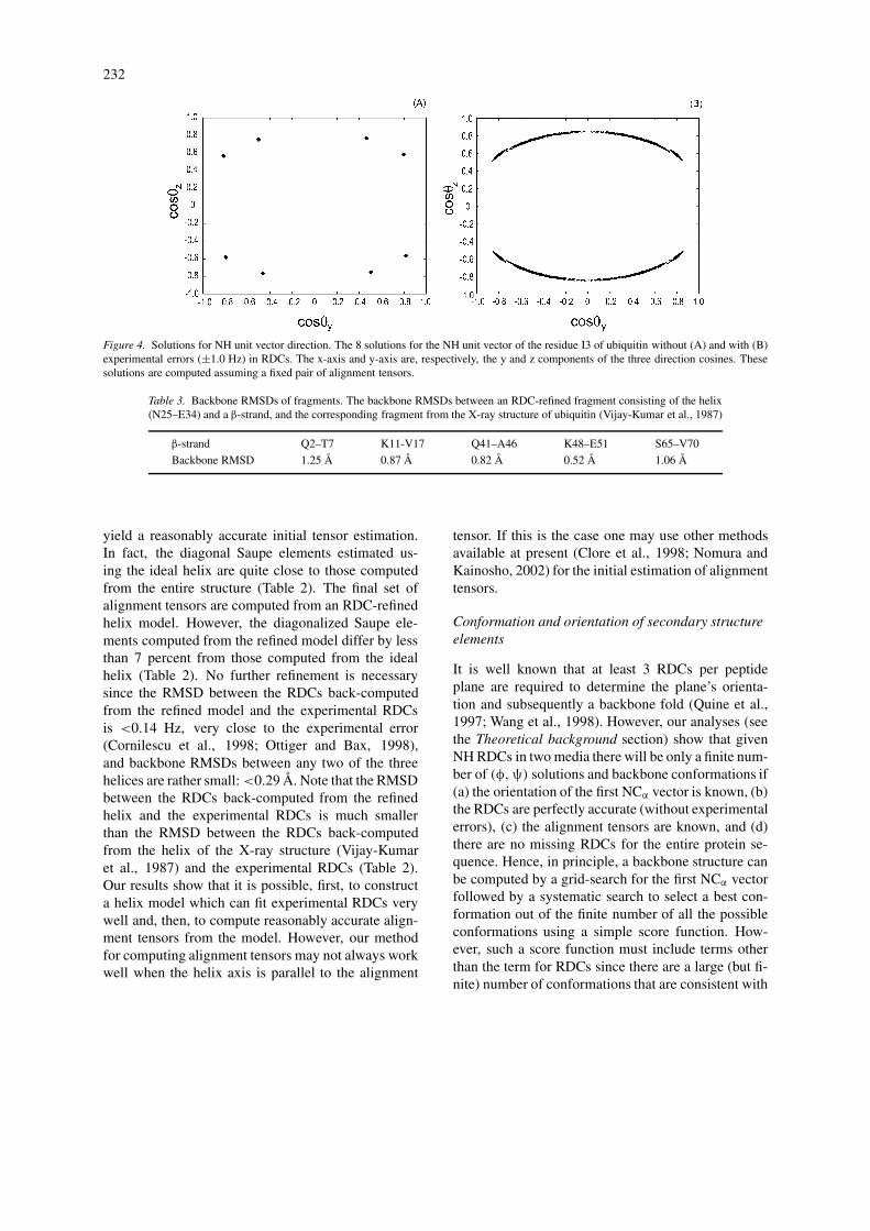
where the coefficients f0, f1, f2, f3, f4 and a are com-puted from S, S′ and R12 which, in turn, can becomputed from the alignment tensors as detailed inthe Computation of alignment tensors section. Fullexpressions for these coefficients are provided in Ap-pendix A. From a given x, y can be computed directlyfrom Equation (1) by solving a quadratic equation.Due to symmetry in Equations (1, 2) the number ofreal solutions for v is at most 8 (Figure 4A), in agree-ment with what has been found previously by othermethods (Al-Hashimi et al., 2000; Ramirez and Bax,1998).

225

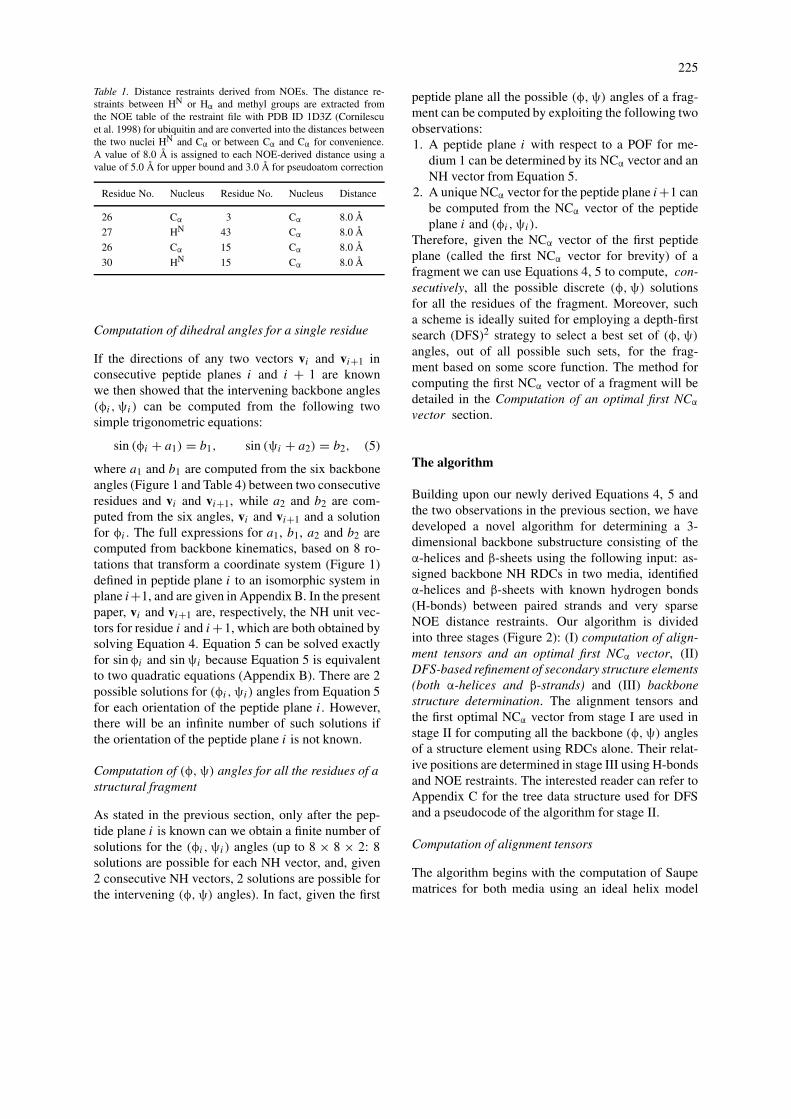
Table 1. Distance restraints derived from NOEs. The distance re-straints between HN or Hα and methyl groups are extracted fromthe NOE table of the restraint file with PDB ID 1D3Z (Cornilescuet al. 1998) for ubiquitin and are converted into the distances betweenthe two nuclei HN and Cα or between Cα and Cα for convenience.A value of 8.0 Å is assigned to each NOE-derived distance using avalue of 5.0 Å for upper bound and 3.0 Å for pseudoatom correction

Residue No. Nucleus Residue No. Nucleus Distance

26 Cα 3 Cα 8.0 Å

27 HN 43 Cα 8.0 Å

26 Cα 15 Cα 8.0 Å

30 HN 15 Cα 8.0 Å

Computation of dihedral angles for a single residue

If the directions of any two vectors vi and vi+1 inconsecutive peptide planes i and i + 1 are knownwe then showed that the intervening backbone angles(φi ,ψi ) can be computed from the following twosimple trigonometric equations:

sin (φi + a1) = b1, sin (ψi + a2) = b2, (5)

where a1 and b1 are computed from the six backboneangles (Figure 1 and Table 4) between two consecutiveresidues and vi and vi+1, while a2 and b2 are com-puted from the six angles, vi and vi+1 and a solutionfor φi . The full expressions for a1, b1, a2 and b2 arecomputed from backbone kinematics, based on 8 ro-tations that transform a coordinate system (Figure 1)defined in peptide plane i to an isomorphic system inplane i+1, and are given in Appendix B. In the presentpaper, vi and vi+1 are, respectively, the NH unit vec-tors for residue i and i +1, which are both obtained bysolving Equation 4. Equation 5 can be solved exactlyfor sin φi and sin ψi because Equation 5 is equivalentto two quadratic equations (Appendix B). There are 2possible solutions for (φi ,ψi ) angles from Equation 5for each orientation of the peptide plane i. However,there will be an infinite number of such solutions ifthe orientation of the peptide plane i is not known.

Computation of (φ,ψ) angles for all the residues of astructural fragment

As stated in the previous section, only after the pep-tide plane i is known can we obtain a finite number ofsolutions for the (φi ,ψi ) angles (up to 8 × 8 × 2: 8solutions are possible for each NH vector, and, given2 consecutive NH vectors, 2 solutions are possible forthe intervening (φ,ψ) angles). In fact, given the first

peptide plane all the possible (φ,ψ) angles of a frag-ment can be computed by exploiting the following twoobservations:1. A peptide plane i with respect to a POF for me-

dium 1 can be determined by its NCα vector and anNH vector from Equation 5.

2. A unique NCα vector for the peptide plane i+1 canbe computed from the NCα vector of the peptideplane i and (φi ,ψi ).

Therefore, given the NCα vector of the first peptideplane (called the first NCα vector for brevity) of afragment we can use Equations 4, 5 to compute, con-secutively, all the possible discrete (φ,ψ) solutionsfor all the residues of the fragment. Moreover, sucha scheme is ideally suited for employing a depth-firstsearch (DFS)2 strategy to select a best set of (φ,ψ)

angles, out of all possible such sets, for the frag-ment based on some score function. The method forcomputing the first NCα vector of a fragment will bedetailed in the Computation of an optimal first NCα

vector section.

The algorithm

Building upon our newly derived Equations 4, 5 andthe two observations in the previous section, we havedeveloped a novel algorithm for determining a 3-dimensional backbone substructure consisting of theα-helices and β-sheets using the following input: as-signed backbone NH RDCs in two media, identifiedα-helices and β-sheets with known hydrogen bonds(H-bonds) between paired strands and very sparseNOE distance restraints. Our algorithm is dividedinto three stages (Figure 2): (I) computation of align-ment tensors and an optimal first NCα vector, (II)DFS-based refinement of secondary structure elements(both α-helices and β-strands) and (III) backbonestructure determination. The alignment tensors andthe first optimal NCα vector from stage I are used instage II for computing all the backbone (φ,ψ) anglesof a structure element using RDCs alone. Their relat-ive positions are determined in stage III using H-bondsand NOE restraints. The interested reader can refer toAppendix C for the tree data structure used for DFSand a pseudocode of the algorithm for stage II.

Computation of alignment tensors

The algorithm begins with the computation of Saupematrices for both media using an ideal helix model

226

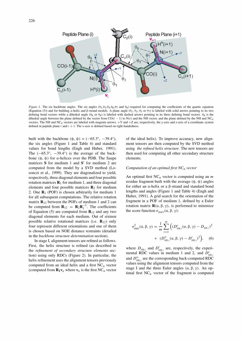
Figure 1. The six backbone angles. The six angles (θ1,θ3,θ5,θ6,θ7 and θ8) required for computing the coefficients of the quartic equation(Equation (5)) and for building α-helix and β-strand models. A plane angle (θ1, θ3, θ5 or θ7) is labeled with solid arrows pointing to its twodefining bond vectors while a dihedral angle (θ6 or θ8) is labeled with dashed arrows pointing to its three defining bond vectors. θ8 is thedihedral angle between the plane defined by the vector from CO(i − 1) to N(i) and the NH vector, and the plane defined by the NH and NCα

vectors. The NH and NCα vectors are labeled with magenta arrows. +Y and +Z are, respectively, the y-axis and z-axis of a coordinate systemdefined in peptide plane i and i + 1. The x-axis is defined based on right handedness.

built with the backbone (φ,ψ) = (−65.3◦, −39.4◦),the six angles (Figure 1 and Table 4) and standardvalues for bond lengths (Engh and Huber, 1991).The (−65.3◦, −39.4◦) is the average of the back-bone (φ,ψ) for α-helices over the PDB. The Saupematrices S for medium 1 and S′ for medium 2 arecomputed from the model by a SVD method (Lo-sonczi et al., 1999). They are diagonalized to yield,respectively, three diagonal elements and four possiblerotation matrices R1 for medium 1, and three diagonalelements and four possible matrices R2 for medium2. One R1 (POF) is chosen arbitrarily for medium 1for all subsequent computations. The relative rotationmatrix R12 between the POFs of medium 1 and 2 canbe computed from R12 = R2R−1

1 . The coefficientsof Equation (5) are computed from R12 and any twodiagonal elements for each medium. Out of sixteenpossible relative rotational matrices (i.e. R12) onlyfour represent different orientations and one of themis chosen based on NOE distance restraints (detailedin the backbone structure determination section).

In stage I, alignment tensors are refined as follows.First, the helix structure is refined (as described inthe refinement of secondary structure elements sec-tion) using only RDCs (Figure 2). In particular, thehelix refinement uses the alignment tensors previouslycomputed from an ideal helix and a first NCα vector(computed from R1vn where vn is the first NCα vector

of the ideal helix). To improve accuracy, new align-ment tensors are then computed by the SVD methodusing the refined helix structure. The new tensors arethen used for computing all other secondary structureelements.

Computation of an optimal first NCα vector

An optimal first NCα vector is computed using an m

residue fragment built with the average (φ,ψ) anglesfor either an α-helix or a β-strand and standard bondlengths and angles (Figure 1 and Table 4) (Engh andHuber, 1991). A grid search for the orientation of thefragment in a POF of medium 1, defined by a Eulerrotation matrix R(α, β, γ), is performed to minimizethe score function σRMS (α, β, γ):

σ2RMS

(α, β, γ) = 1

m

m∑i=1

((Dc

NH,i(α, β, γ) − DNH,i)

2

+ (D′cNH,i

(α, β, γ) − D′NH,i

)2), (6)

where DNH,i and D′NH,i

are, respectively, the experi-mental RDC values in medium 1 and 2, and Dc

NH,i

and D′cNH,i

are the corresponding back-computed RDCvalues using the alignment tensors computed from thestage I and the three Euler angles (α, β, γ). An op-timal first NCα vector of the fragment is computed

227

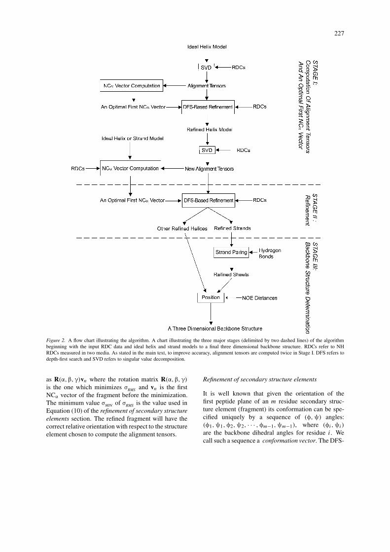
Figure 2. A flow chart illustrating the algorithm. A chart illustrating the three major stages (delimited by two dashed lines) of the algorithmbeginning with the input RDC data and ideal helix and strand models to a final three dimensional backbone structure. RDCs refer to NHRDCs measured in two media. As stated in the main text, to improve accuracy, alignment tensors are computed twice in Stage I. DFS refers todepth-first search and SVD refers to singular value decomposition.

as R(α, β, γ)vn where the rotation matrix R(α, β, γ)

is the one which minimizes σRMS and vn is the firstNCα vector of the fragment before the minimization.The minimum value σMIN of σRMS is the value used inEquation (10) of the refinement of secondary structureelements section. The refined fragment will have thecorrect relative orientation with respect to the structureelement chosen to compute the alignment tensors.

Refinement of secondary structure elements

It is well known that given the orientation of thefirst peptide plane of an m residue secondary struc-ture element (fragment) its conformation can be spe-cified uniquely by a sequence of (φ,ψ) angles:(φ1,ψ1,φ2,ψ2, · · · ,φm−1,ψm−1), where (φi ,ψi )

are the backbone dihedral angles for residue i. Wecall such a sequence a conformation vector. The DFS-

228

based refinement (stage II) is a minimization searchingsystematically for an NH vector of the first peptideplane (since an optimal first NCα vector has beendetermined) and a conformation vector such that themodel built from the first peptide plane and the con-formation vector has (a) (φ,ψ) values as close aspossible to the average (φa,ψa) over the PDB for thecorresponding secondary structure type and (b) sim-ultaneously fits the experimental RDC data as wellas possible. We call such a conformation vector anoptimal conformation vector. What we mean by re-finement here is to optimize both the direction ofindividual NH vectors and also the (φ,ψ) angles ofa fragment using only RDCs while leaving the bondlengths and the six angles (Table 1 and Figure 4) fixed.Formally, our algorithm minimizes a score functionT1:

T1 =m−1∑i=1

((φi − φa)

2 + (ψi − ψa)2)

+m∑

i=1

((Ds

NH,i− DNH,i

)2

+(D′s

NH,i− D′

NH,i

)2)

, (7)

for a helix or a β-strand of a sheet chosen to be builtfirst. For the other β-strands of the sheet it minimizesa score function T2:

T2 =m−1∑i=1

((φi − φa)

2 + (ψi − ψa)2)

+m∑

i=1

((Ds

NH,i− DNH,i

)2

+(D′s

NH,i− D′

NH,i

)2)

+ TH , (8)

where

TH(φ1,ψ1, · · · ,φm−1,ψm−1) =

q∑j=1

((H

L,j− H

L,a

)2 + (H

A,j− H

A,a

)2)

, (9)

and where DNH,i and D′NH,i

are, respectively, the ex-perimental RDC values in medium 1 and 2, Ds

NH,iand

D′sNH,i

are the corresponding RDC values sampled fromGaussian distributions simulating the experimental er-rors (the experimental value and error are, respect-ively, the mean and variance), H

L,jand H

A,jare,

respectively, the computed H-bond length and angle,and HL,a and HA,a are the corresponding values for an

ideal H-bond, and q is the number of H-bonds betweenthe paired strands. During the refinement φa , ψa ,DNH,i , D′

NH,i, HL,a and HA,a are treated as constants

while DsNH,i

, D′sNH,i

and the φi , ψi angles computedfrom them are treated as variables.

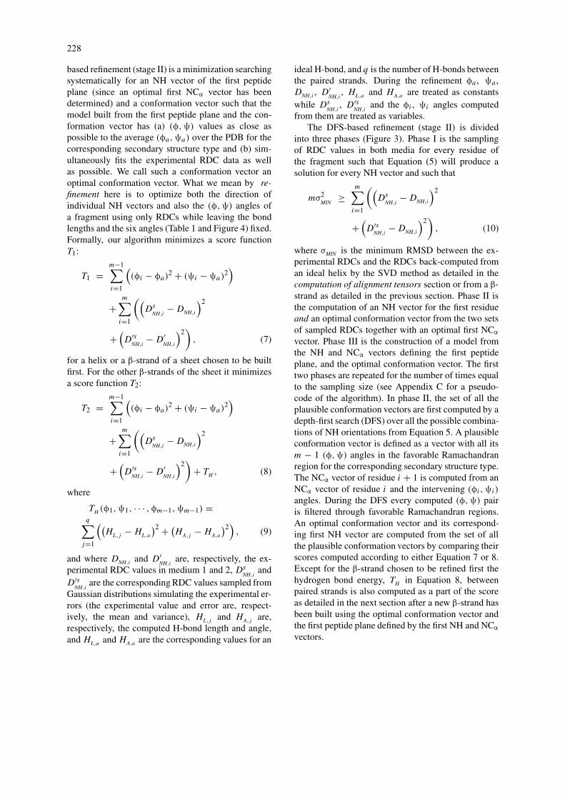
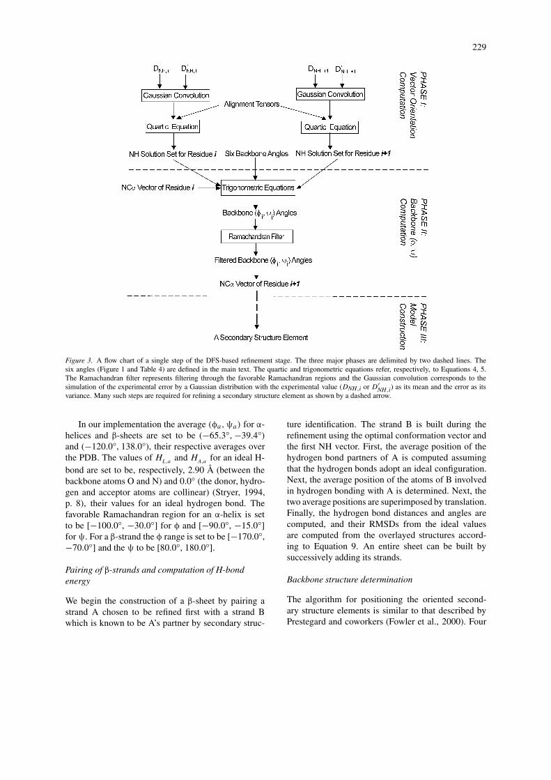
The DFS-based refinement (stage II) is dividedinto three phases (Figure 3). Phase I is the samplingof RDC values in both media for every residue ofthe fragment such that Equation (5) will produce asolution for every NH vector and such that

mσ2MIN

≥m∑

i=1

((Ds

NH,i− DNH,i

)2

+(D′s

NH,i− DNH,i

)2)

, (10)

where σMIN is the minimum RMSD between the ex-perimental RDCs and the RDCs back-computed froman ideal helix by the SVD method as detailed in thecomputation of alignment tensors section or from a β-strand as detailed in the previous section. Phase II isthe computation of an NH vector for the first residueand an optimal conformation vector from the two setsof sampled RDCs together with an optimal first NCα

vector. Phase III is the construction of a model fromthe NH and NCα vectors defining the first peptideplane, and the optimal conformation vector. The firsttwo phases are repeated for the number of times equalto the sampling size (see Appendix C for a pseudo-code of the algorithm). In phase II, the set of all theplausible conformation vectors are first computed by adepth-first search (DFS) over all the possible combina-tions of NH orientations from Equation 5. A plausibleconformation vector is defined as a vector with all itsm − 1 (φ,ψ) angles in the favorable Ramachandranregion for the corresponding secondary structure type.The NCα vector of residue i + 1 is computed from anNCα vector of residue i and the intervening (φi ,ψi )

angles. During the DFS every computed (φ,ψ) pairis filtered through favorable Ramachandran regions.An optimal conformation vector and its correspond-ing first NH vector are computed from the set of allthe plausible conformation vectors by comparing theirscores computed according to either Equation 7 or 8.Except for the β-strand chosen to be refined first thehydrogen bond energy, TH in Equation 8, betweenpaired strands is also computed as a part of the scoreas detailed in the next section after a new β-strand hasbeen built using the optimal conformation vector andthe first peptide plane defined by the first NH and NCα

vectors.

229

Figure 3. A flow chart of a single step of the DFS-based refinement stage. The three major phases are delimited by two dashed lines. Thesix angles (Figure 1 and Table 4) are defined in the main text. The quartic and trigonometric equations refer, respectively, to Equations 4, 5.The Ramachandran filter represents filtering through the favorable Ramachandran regions and the Gaussian convolution corresponds to thesimulation of the experimental error by a Gaussian distribution with the experimental value (DNH,i or D′

NH,i) as its mean and the error as itsvariance. Many such steps are required for refining a secondary structure element as shown by a dashed arrow.

In our implementation the average (φa,ψa) for α-helices and β-sheets are set to be (−65.3◦, −39.4◦)and (−120.0◦, 138.0◦), their respective averages overthe PDB. The values of H

L,aand H

A,afor an ideal H-

bond are set to be, respectively, 2.90 Å (between thebackbone atoms O and N) and 0.0◦ (the donor, hydro-gen and acceptor atoms are collinear) (Stryer, 1994,p. 8), their values for an ideal hydrogen bond. Thefavorable Ramachandran region for an α-helix is setto be [−100.0◦, −30.0◦] for φ and [−90.0◦, −15.0◦]for ψ. For a β-strand the φ range is set to be [−170.0◦,−70.0◦] and the ψ to be [80.0◦, 180.0◦].

Pairing of β-strands and computation of H-bondenergy

We begin the construction of a β-sheet by pairing astrand A chosen to be refined first with a strand Bwhich is known to be A’s partner by secondary struc-

ture identification. The strand B is built during therefinement using the optimal conformation vector andthe first NH vector. First, the average position of thehydrogen bond partners of A is computed assumingthat the hydrogen bonds adopt an ideal configuration.Next, the average position of the atoms of B involvedin hydrogen bonding with A is determined. Next, thetwo average positions are superimposed by translation.Finally, the hydrogen bond distances and angles arecomputed, and their RMSDs from the ideal valuesare computed from the overlayed structures accord-ing to Equation 9. An entire sheet can be built bysuccessively adding its strands.

Backbone structure determination

The algorithm for positioning the oriented second-ary structure elements is similar to that described byPrestegard and coworkers (Fowler et al., 2000). Four

230

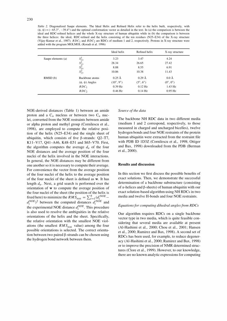
Table 2. Diagonalized Saupe elements. The Ideal Helix and Refined Helix refer to the helix built, respectively, with(φ,ψ) = (−65.3◦, −39.4◦) and the optimal conformation vector as detailed in the text. In (a) the comparison is between theideal and RDC-refined helices and the whole X-ray structure of human ubiquitin while in (b) the comparison is betweenthe three helices: the ideal, RDC-refined and the helix consisting of the ten residues (N25–E34) of the X-ray structure(Vijay-Kumar et al., 1987). RDC1 and RDC2 are RDCs of medium 1 and 2, respectively. Protons in X-ray structure wereadded with the program MOLMOL (Koradi et al. 1996)

Ideal helix Refined helix X-ray structure

Saupe elements (a) S1xx 3.23 3.47 4.24

S1yy 28.34 26.65 27.42

S2xx 8.88 8.55 6.91

S2yy 10.06 10.38 11.43

RMSD (b) Backbone atoms 0.25 Å 0.29 Å 0.0 Å

(φ,ψ) Angles (10◦, 9◦) (5◦, 6◦) (0◦, 0◦)

RDC1 0.39 Hz 0.12 Hz 1.43 Hz

RDC2 0.46 Hz 0.14 Hz 0.95 Hz

NOE-derived distances (Table 1) between an amideproton and a Cα nucleus or between two Cα nuc-lei, converted from the NOE restraints between amideor alpha proton and methyl group (Cornilescu et al.,1998), are employed to compute the relative posi-tion of the helix (N25–E34) and the single sheet ofubiquitin, which consists of five β-strands: Q2–T7,K11–V17, Q41–A46, K48–E51 and S65–V70. First,the algorithm computes the average da of the fourNOE distances and the average position of the fournuclei of the helix involved in the NOE interactions.In general, the NOE distances may be different fromone another so it is necessary to compute their average.For convenience the vector from the average positionof the four nuclei of the helix to the average positionof the four nuclei of the sheet is defined as w. It haslength da . Next, a grid search is performed over theorientation of w to compute the average position ofthe four nuclei of the sheet (the position of the helix isfixed here) to minimize the RMSNOE = ∑4

i=1(d′NOEi −

dNOEi )2 between the computed distances d ′NOE

i andthe experimental NOE distance dNOE

i . This procedureis also used to resolve the ambiguities in the relativeorientations of the helix and the sheet. Specifically,the relative orientation with the smallest NOE viol-ations (the smallest RMSNOE value) among the fourpossible orientations is selected. The correct orienta-tion between two paired β-strands can be chosen usingthe hydrogen bond network between them.

Source of the data

The backbone NH RDC data in two different media(medium 1 and 2 correspond, respectively, to thosemeasured in charged and uncharged bicelles), twelvehydrogen bonds and four NOE restraints of the proteinhuman ubiquitin were extracted from the restraint filewith PDB ID 1D3Z (Cornilescu et al., 1998; Ottigerand Bax, 1998) downloaded from the PDB (Bermanet al., 2000).

Results and discussion

In this section we first discuss the possible benefits ofexact solutions. Then, we demonstrate the successfuldetermination of a backbone substructure (consistingof α-helices and β-sheets) of human ubiquitin with ourexact solution-based algorithm using NH RDCs in twomedia and twelve H-bonds and four NOE restraints.

Equations for computing dihedral angles from RDCs

Our algorithm requires RDCs on a single backbonevector type in two media, which is quite feasible con-sidering that several media are available at present(Al-Hashimi et al., 2000; Chou et al., 2001; Hansenet al., 2000; Ramirez and Bax, 1998). A second set ofRDCs has been used, for example, to reduce degener-acy (Al-Hashimi et al., 2000; Ramirez and Bax, 1998)or to improve the precision of NMR determined struc-tures (Clore et al., 1999). However, to our knowledge,there are no known analytic expressions for computing

231

either internuclear vectors or backbone (φ,ψ) anglesdirectly from RDCs when the POFs of medium 1 and2 are not identical. Previously, numerical fitting hasbeen used to compute NH vector orientations (Bar-bieri et al., 2002) and 2-dimensional grid-search hasbeen used to determine (φ,ψ) angles (Giesen et al.,2003; Tian et al., 2001; Wang et al., 1998) when RDCsare measured on at least three backbone vector types.Scheraga and coworkers (Wedemeyer et al., 2002)have derived a quartic equation for computing vectororientations when the two POFs are identical. Forthe general case when the two POFs are different theysuggest using 1-dimensional grid search to computevector orientations. Griesinger and coworkers (Meileret al., 2000) have derived an expression for computingpairwise angular restraints between internuclear vec-tors whose RDCs are measured in one medium. Incontrast, our equations (Equations 4, 5) are derivedto compute, exactly, the intervening backbone dihed-ral angles between two consecutive residues whoseNH RDCs have been measured in two media. Theycan not be used to compute the inter-vector anglebetween two NH vectors. The advantages of exactsolution methods have been demonstrated by Crossand coworkers (Bertram et al., 2000) for comput-ing solid-state NMR structures and by Scheraga andcoworkers (Wedemeyer et al., 2002) for computingsolution NMR structures. The possible benefits ofexact methods include:1. Exact solutions make it possible to characterize

the properties of the solutions. For example, thenumber of solutions from Equation 5 can be 0,2, 4, 6 or 8, in agreement with the previous res-ults obtained by other methods (Al-Hashimi et al.,2000; Ramirez and Bax, 1998; Wedemeyer et al.,2002) (Figure 4A). Further, the average number ofreal solutions (as opposed to complex) is close to4, in agreement with what has been known in al-gebraic geometry (Kac, 1948). Given the peptideplane i the two possible (φi ,ψi ) solutions fromEquation 5 have very similar φi values (differingby <10◦) but with opposite sign if the coefficientsof Equation 5 are computed using the averagesfor the six angles (Table 4). In our implementa-tion these average values were obtained from 23ultra-high resolution X-ray structures with protoncoordinates (Table 4). Consequently, except forglycine, all residues located in regular α-helicesand β-sheets have only one (φ,ψ) solution in thefavorable Ramachandran regions. And the solutionwith positive φ value can be safely discarded for

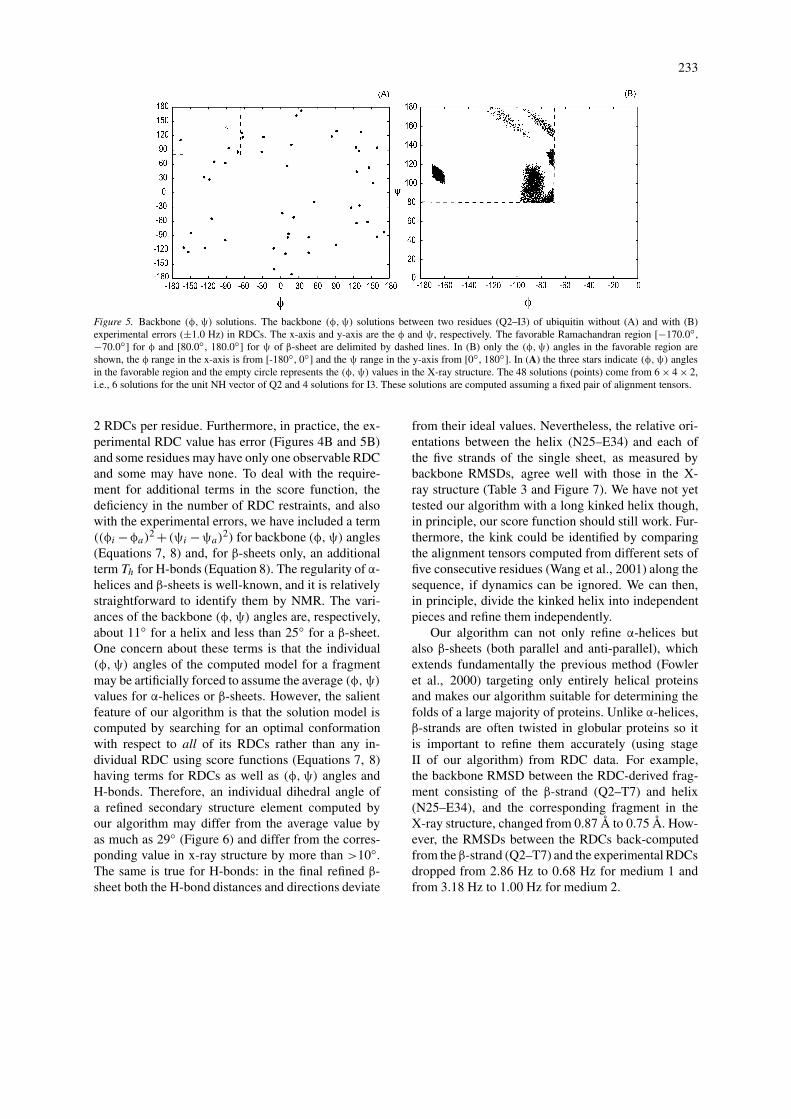
a residue in regular α-helix or β-strand. Further,for most residues in regular α-helices and β-sheets,only a few of the 8×8×2 possible (φ,ψ) solutionswill fall into the favorable regions (Figure 5A).

2. With exact solutions it is possible to quantifythe contributions to the accuracy of the computed(φ,ψ) angles from both the experimental errors inRDCs (Figure 5B) and the statistical distributionsof the six angles (Table 4) required as additionalrestraints in Equation 5. Among the six angles, thedihedral angle θ6 (Table 4 and Figure 1), whichmeasures the deviation of an NH vector from thepeptide plane, has the largest variance (6.0◦) whilethe other five have much smaller variances (<2.4◦)(Table 4). Our results from exact solutions showthat the variation of this angle does not change theφi value and only changes ψi by <10◦.

3. Exact solutions are expected to be useful for speed-ing up the structure determination of both proteinsand nucleic acids using RDC and/or pseudocon-tact shift restraints (Kemple et al., 1988) sincesimilar equations can be derived for computingthe corresponding vector orientation and dihedralangle. As a demonstration we have shown (see theConformation and orientation of secondary struc-ture elements section) that such exact solutionsmake it feasible and efficient to search system-atically through all the possible combinations of(φ,ψ) solutions for a secondary structure elementto determine a conformation that best satisfies boththe experimental RDCs and has backbone (φ,ψ)

values as close as possible to the PDB averages(Equation 7 or 8).

Computation of alignment tensors

For alignment tensor computation we take the advant-age of a priori knowledge about secondary structureelements. Specifically, we select a helix model con-sisting of residues N25–E34 to be built and refinedfirst for their computation. In general, helices can beidentified easily, have less variations in local structurethan β-sheets do, are more stable, and their amideprotons are less labile than those in loops so theexperimental data have smaller errors (Wang et al.,2001). Some concerns (Fowler et al., 2000) have beenraised about the accuracy of the computed Saupe mat-rix because the NH bond vectors are near parallel ina regular helix. However, our results show that thevariations in NH orientations in the ideal helix builtwith (φ,ψ) = (−65.3◦, −39.4◦) are large enough to

232

Figure 4. Solutions for NH unit vector direction. The 8 solutions for the NH unit vector of the residue I3 of ubiquitin without (A) and with (B)experimental errors (±1.0 Hz) in RDCs. The x-axis and y-axis are, respectively, the y and z components of the three direction cosines. Thesesolutions are computed assuming a fixed pair of alignment tensors.

Table 3. Backbone RMSDs of fragments. The backbone RMSDs between an RDC-refined fragment consisting of the helix(N25–E34) and a β-strand, and the corresponding fragment from the X-ray structure of ubiquitin (Vijay-Kumar et al., 1987)

β-strand Q2–T7 K11-V17 Q41–A46 K48–E51 S65–V70

Backbone RMSD 1.25 Å 0.87 Å 0.82 Å 0.52 Å 1.06 Å

yield a reasonably accurate initial tensor estimation.In fact, the diagonal Saupe elements estimated us-ing the ideal helix are quite close to those computedfrom the entire structure (Table 2). The final set ofalignment tensors are computed from an RDC-refinedhelix model. However, the diagonalized Saupe ele-ments computed from the refined model differ by lessthan 7 percent from those computed from the idealhelix (Table 2). No further refinement is necessarysince the RMSD between the RDCs back-computedfrom the refined model and the experimental RDCsis <0.14 Hz, very close to the experimental error(Cornilescu et al., 1998; Ottiger and Bax, 1998),and backbone RMSDs between any two of the threehelices are rather small: <0.29 Å. Note that the RMSDbetween the RDCs back-computed from the refinedhelix and the experimental RDCs is much smallerthan the RMSD between the RDCs back-computedfrom the helix of the X-ray structure (Vijay-Kumaret al., 1987) and the experimental RDCs (Table 2).Our results show that it is possible, first, to constructa helix model which can fit experimental RDCs verywell and, then, to compute reasonably accurate align-ment tensors from the model. However, our methodfor computing alignment tensors may not always workwell when the helix axis is parallel to the alignment

tensor. If this is the case one may use other methodsavailable at present (Clore et al., 1998; Nomura andKainosho, 2002) for the initial estimation of alignmenttensors.

Conformation and orientation of secondary structureelements

It is well known that at least 3 RDCs per peptideplane are required to determine the plane’s orienta-tion and subsequently a backbone fold (Quine et al.,1997; Wang et al., 1998). However, our analyses (seethe Theoretical background section) show that givenNH RDCs in two media there will be only a finite num-ber of (φ,ψ) solutions and backbone conformations if(a) the orientation of the first NCα vector is known, (b)the RDCs are perfectly accurate (without experimentalerrors), (c) the alignment tensors are known, and (d)there are no missing RDCs for the entire protein se-quence. Hence, in principle, a backbone structure canbe computed by a grid-search for the first NCα vectorfollowed by a systematic search to select a best con-formation out of the finite number of all the possibleconformations using a simple score function. How-ever, such a score function must include terms otherthan the term for RDCs since there are a large (but fi-nite) number of conformations that are consistent with

233

Figure 5. Backbone (φ,ψ) solutions. The backbone (φ,ψ) solutions between two residues (Q2–I3) of ubiquitin without (A) and with (B)experimental errors (±1.0 Hz) in RDCs. The x-axis and y-axis are the φ and ψ, respectively. The favorable Ramachandran region [−170.0◦,−70.0◦] for φ and [80.0◦, 180.0◦] for ψ of β-sheet are delimited by dashed lines. In (B) only the (φ,ψ) angles in the favorable region areshown, the φ range in the x-axis is from [-180◦, 0◦] and the ψ range in the y-axis from [0◦, 180◦]. In (A) the three stars indicate (φ,ψ) anglesin the favorable region and the empty circle represents the (φ,ψ) values in the X-ray structure. The 48 solutions (points) come from 6 × 4 × 2,i.e., 6 solutions for the unit NH vector of Q2 and 4 solutions for I3. These solutions are computed assuming a fixed pair of alignment tensors.

2 RDCs per residue. Furthermore, in practice, the ex-perimental RDC value has error (Figures 4B and 5B)and some residues may have only one observable RDCand some may have none. To deal with the require-ment for additional terms in the score function, thedeficiency in the number of RDC restraints, and alsowith the experimental errors, we have included a term((φi −φa)

2 + (ψi −ψa)2) for backbone (φ,ψ) angles

(Equations 7, 8) and, for β-sheets only, an additionalterm Th for H-bonds (Equation 8). The regularity of α-helices and β-sheets is well-known, and it is relativelystraightforward to identify them by NMR. The vari-ances of the backbone (φ,ψ) angles are, respectively,about 11◦ for a helix and less than 25◦ for a β-sheet.One concern about these terms is that the individual(φ,ψ) angles of the computed model for a fragmentmay be artificially forced to assume the average (φ,ψ)

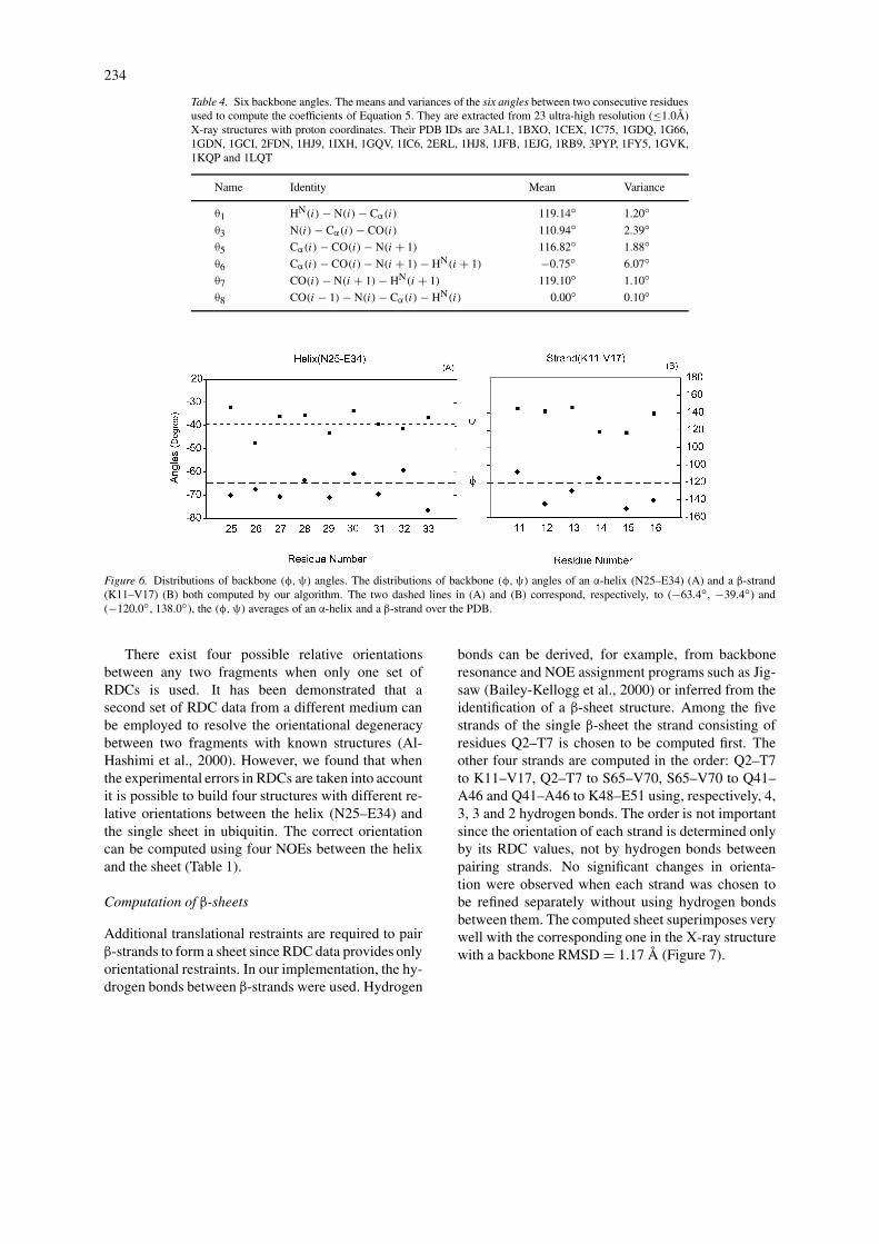
values for α-helices or β-sheets. However, the salientfeature of our algorithm is that the solution model iscomputed by searching for an optimal conformationwith respect to all of its RDCs rather than any in-dividual RDC using score functions (Equations 7, 8)having terms for RDCs as well as (φ,ψ) angles andH-bonds. Therefore, an individual dihedral angle ofa refined secondary structure element computed byour algorithm may differ from the average value byas much as 29◦ (Figure 6) and differ from the corres-ponding value in x-ray structure by more than >10◦.The same is true for H-bonds: in the final refined β-sheet both the H-bond distances and directions deviate

from their ideal values. Nevertheless, the relative ori-entations between the helix (N25–E34) and each ofthe five strands of the single sheet, as measured bybackbone RMSDs, agree well with those in the X-ray structure (Table 3 and Figure 7). We have not yettested our algorithm with a long kinked helix though,in principle, our score function should still work. Fur-thermore, the kink could be identified by comparingthe alignment tensors computed from different sets offive consecutive residues (Wang et al., 2001) along thesequence, if dynamics can be ignored. We can then,in principle, divide the kinked helix into independentpieces and refine them independently.

Our algorithm can not only refine α-helices butalso β-sheets (both parallel and anti-parallel), whichextends fundamentally the previous method (Fowleret al., 2000) targeting only entirely helical proteinsand makes our algorithm suitable for determining thefolds of a large majority of proteins. Unlike α-helices,β-strands are often twisted in globular proteins so itis important to refine them accurately (using stageII of our algorithm) from RDC data. For example,the backbone RMSD between the RDC-derived frag-ment consisting of the β-strand (Q2–T7) and helix(N25–E34), and the corresponding fragment in theX-ray structure, changed from 0.87 Å to 0.75 Å. How-ever, the RMSDs between the RDCs back-computedfrom the β-strand (Q2–T7) and the experimental RDCsdropped from 2.86 Hz to 0.68 Hz for medium 1 andfrom 3.18 Hz to 1.00 Hz for medium 2.

234

Table 4. Six backbone angles. The means and variances of the six angles between two consecutive residuesused to compute the coefficients of Equation 5. They are extracted from 23 ultra-high resolution (≤1.0Å)X-ray structures with proton coordinates. Their PDB IDs are 3AL1, 1BXO, 1CEX, 1C75, 1GDQ, 1G66,1GDN, 1GCI, 2FDN, 1HJ9, 1IXH, 1GQV, 1IC6, 2ERL, 1HJ8, 1JFB, 1EJG, 1RB9, 3PYP, 1FY5, 1GVK,1KQP and 1LQT

Name Identity Mean Variance

θ1 HN(i) − N(i) − Cα(i) 119.14◦ 1.20◦θ3 N(i) − Cα(i) − CO(i) 110.94◦ 2.39◦θ5 Cα(i) − CO(i) − N(i + 1) 116.82◦ 1.88◦θ6 Cα(i) − CO(i) − N(i + 1) − HN(i + 1) −0.75◦ 6.07◦θ7 CO(i) − N(i + 1) − HN(i + 1) 119.10◦ 1.10◦θ8 CO(i − 1) − N(i) − Cα(i) − HN(i) 0.00◦ 0.10◦

Figure 6. Distributions of backbone (φ,ψ) angles. The distributions of backbone (φ,ψ) angles of an α-helix (N25–E34) (A) and a β-strand(K11–V17) (B) both computed by our algorithm. The two dashed lines in (A) and (B) correspond, respectively, to (−63.4◦, −39.4◦) and(−120.0◦, 138.0◦), the (φ,ψ) averages of an α-helix and a β-strand over the PDB.

There exist four possible relative orientationsbetween any two fragments when only one set ofRDCs is used. It has been demonstrated that asecond set of RDC data from a different medium canbe employed to resolve the orientational degeneracybetween two fragments with known structures (Al-Hashimi et al., 2000). However, we found that whenthe experimental errors in RDCs are taken into accountit is possible to build four structures with different re-lative orientations between the helix (N25–E34) andthe single sheet in ubiquitin. The correct orientationcan be computed using four NOEs between the helixand the sheet (Table 1).

Computation of β-sheets

Additional translational restraints are required to pairβ-strands to form a sheet since RDC data provides onlyorientational restraints. In our implementation, the hy-drogen bonds between β-strands were used. Hydrogen

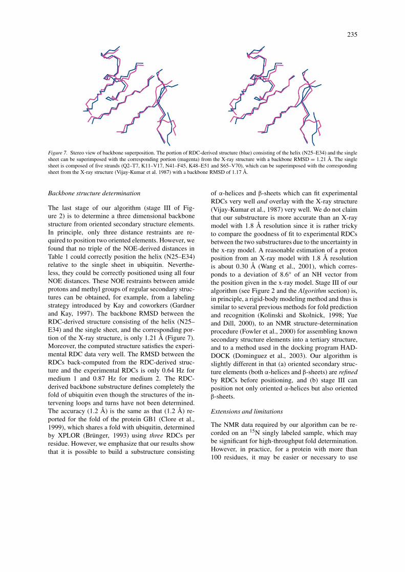
bonds can be derived, for example, from backboneresonance and NOE assignment programs such as Jig-saw (Bailey-Kellogg et al., 2000) or inferred from theidentification of a β-sheet structure. Among the fivestrands of the single β-sheet the strand consisting ofresidues Q2–T7 is chosen to be computed first. Theother four strands are computed in the order: Q2–T7to K11–V17, Q2–T7 to S65–V70, S65–V70 to Q41–A46 and Q41–A46 to K48–E51 using, respectively, 4,3, 3 and 2 hydrogen bonds. The order is not importantsince the orientation of each strand is determined onlyby its RDC values, not by hydrogen bonds betweenpairing strands. No significant changes in orienta-tion were observed when each strand was chosen tobe refined separately without using hydrogen bondsbetween them. The computed sheet superimposes verywell with the corresponding one in the X-ray structurewith a backbone RMSD = 1.17 Å (Figure 7).

235

Figure 7. Stereo view of backbone superposition. The portion of RDC-derived structure (blue) consisting of the helix (N25–E34) and the singlesheet can be superimposed with the corresponding portion (magenta) from the X-ray structure with a backbone RMSD = 1.21 Å. The singlesheet is composed of five strands (Q2–T7, K11–V17, N41–F45, K48–E51 and S65–V70), which can be superimposed with the correspondingsheet from the X-ray structure (Vijay-Kumar et al. 1987) with a backbone RMSD of 1.17 Å.

Backbone structure determination

The last stage of our algorithm (stage III of Fig-ure 2) is to determine a three dimensional backbonestructure from oriented secondary structure elements.In principle, only three distance restraints are re-quired to position two oriented elements. However, wefound that no triple of the NOE-derived distances inTable 1 could correctly position the helix (N25–E34)relative to the single sheet in ubiquitin. Neverthe-less, they could be correctly positioned using all fourNOE distances. These NOE restraints between amideprotons and methyl groups of regular secondary struc-tures can be obtained, for example, from a labelingstrategy introduced by Kay and coworkers (Gardnerand Kay, 1997). The backbone RMSD between theRDC-derived structure consisting of the helix (N25–E34) and the single sheet, and the corresponding por-tion of the X-ray structure, is only 1.21 Å (Figure 7).Moreover, the computed structure satisfies the experi-mental RDC data very well. The RMSD between theRDCs back-computed from the RDC-derived struc-ture and the experimental RDCs is only 0.64 Hz formedium 1 and 0.87 Hz for medium 2. The RDC-derived backbone substructure defines completely thefold of ubiquitin even though the structures of the in-tervening loops and turns have not been determined.The accuracy (1.2 Å) is the same as that (1.2 Å) re-ported for the fold of the protein GB1 (Clore et al.,1999), which shares a fold with ubiquitin, determinedby XPLOR (Brünger, 1993) using three RDCs perresidue. However, we emphasize that our results showthat it is possible to build a substructure consisting

of α-helices and β-sheets which can fit experimentalRDCs very well and overlay with the X-ray structure(Vijay-Kumar et al., 1987) very well. We do not claimthat our substructure is more accurate than an X-raymodel with 1.8 Å resolution since it is rather trickyto compare the goodness of fit to experimental RDCsbetween the two substructures due to the uncertainty inthe x-ray model. A reasonable estimation of a protonposition from an X-ray model with 1.8 Å resolutionis about 0.30 Å (Wang et al., 2001), which corres-ponds to a deviation of 8.6◦ of an NH vector fromthe position given in the x-ray model. Stage III of ouralgorithm (see Figure 2 and the Algorithm section) is,in principle, a rigid-body modeling method and thus issimilar to several previous methods for fold predictionand recognition (Kolinski and Skolnick, 1998; Yueand Dill, 2000), to an NMR structure-determinationprocedure (Fowler et al., 2000) for assembling knownsecondary structure elements into a tertiary structure,and to a method used in the docking program HAD-DOCK (Dominguez et al., 2003). Our algorithm isslightly different in that (a) oriented secondary struc-ture elements (both α-helices and β-sheets) are refinedby RDCs before positioning, and (b) stage III canposition not only oriented α-helices but also orientedβ-sheets.

Extensions and limitations

The NMR data required by our algorithm can be re-corded on an 15N singly labeled sample, which maybe significant for high-throughput fold determination.However, in practice, for a protein with more than100 residues, it may be easier or necessary to use

236

15N and 13C double labeling to assign backbone reson-ances and to identify secondary structure elements. Infact, with double labeling it is rather straightforwardto measure more than two RDCs per residue. Addi-tional RDCs, if available, can be easily incorporatedinto our algorithm to increase the accuracy of the com-puted (φ,ψ) angles and to eliminate the requirementthat the computed α-helix or β-strand have backbone(φ,ψ) values as close as possible to the PDB averages.The focus of the current paper is to present the deriv-ation of low-degree polynomials used for computing,exactly, the internuclear vector and backbone (φ,ψ)

angles from two RDCs per residue and to demonstratethe possibility of computing a backbone substruc-ture from those RDCs using an algorithm built uponexact solutions and systematic search. In principle,these low-degree polynomials can be easily incorpor-ated into a structure determination algorithm usingrestrained molecular dynamics (MD) in torsion anglespace such as DYANA (Güntert et al., 1997). In fact,a module with NH orientation obtained from RDCsby numerical fitting has been implemented recently inDYANA by Luchinat and coworkers (Barbieri et al.,2002). Compared to the restrained MD with simulatedannealing (SA) approaches (Brünger, 1993; Güntertet al., 1997; Clore et al., 1999; Giesen et al., 2003; Huset al., 2001), the novelty of our algorithm lies in howthe input data (RDCs) are used to limit the searchspace and how a global minimum is computed:1. In our algorithm, the space of solutions is, a pri-

ori, explicitly restricted by the data: first, the spaceof NH internuclear bond vectors is restricted to aset of finite solutions. This, in turn, kinematicallyrestricts the space of backbone dihedral angles toa finite set before a conformation is computed. Incontrast, in restrained MD/SA, the space of solu-tions is implicitly restricted by an energy functionthat penalizes those computed conformations forwhich the back-calculated and experimental RDCsdisagree.

2. In a restrained MD/SA approach, MD is used asa minimization tool to solve a multiple variableminimization problem. Since there are many localminima a heuristic search such as SA is, in gen-eral, used to search for the true global minimum.However, since SA is a non-deterministic, iterativeapproach that samples the search space stochastic-ally, the computed minimum is most likely to beonly a local minimum. In other words, a structurecomputed by such an algorithm is not guaranteedto be the true global minimum even with perfect

data. In contrast, our algorithm is deterministic,non-iterative and combinatorially precise, thus, ifthe input data (experimental RDCs) are perfectlyaccurate (without any experimental error) our sys-tematic search method is guaranteed to find the trueglobal minimum. The advantages of systematicsearch vs. heuristic search have been previouslydescribed (see, for example, Rienstra et al. 2002).

The computational and modeling benefits of exactsolutions have been described by Cross and cowork-ers (Bertram et al., 2000) for computing solid-stateNMR structures and by Scheraga and co-workers (We-demeyer et al., 2002) for computing the backbonestructure of ubiquitin in solution using five RDCsin one medium. However, in the former a Monte-Carlo method is used to search over possible con-formational space and in the latter final structures arerefined by ROSETTA (Rohl and Baker, 2002) whichuses, first, a fragment replacement method (Delaglioet al., 2000) to reduce the search space, then, aMonte-Carlo Method to search over the reduced con-formation space. Systematic search has proved usefulin solid-state NMR structure determination (Rienstraet al., 2002) for a tripeptide. However, Griffin and co-workers did not derive or employ exact solutions. Ouralgorithm is the first NMR structure determination al-gorithm that uses both exact solutions and systematicsearch.

The running time of our algorithm (see AppendixD for an analysis of the algorithmic complexity andperformance), about 45 min for computing a 39-residue substructure of ubiquitin, is comparable tothe time needed by a full-blown structure determina-tion algorithm such as XPLOR (Brünger, 1993) usingmany NOEs and dihedral angle restraints. As is wellknown, a systematic search over the entire solutionspace needs more time than a heuristic search whichsamples the space stochastically. However, with ex-act solutions and a pruning strategy based on theRamachandran plot our algorithm managed to com-pute the substructure of ubiquitin in a comparabletime. Furthermore, months of time could be saved byavoiding the assignments of large number of NOEsinvolving sidechain protons in order to compute an ac-curate structure using a full-blown, traditional method.In addition, hours of spectrometer time may be savedsince fewer NMR experiments are needed and singlelabeling is less expensive than double labeling, ingeneral.

237

Conclusions

We have described a novel algorithm for determininga protein backbone structure by solution NMR spec-troscopy, using almost exclusively angular restraintsfrom RDCs measured on a single bond vector type(NH) in two media, plus very sparse distance re-straints. The algorithm is built upon our newly-derivedequations for computing (φ,ψ) angles, exactly andin constant time, from two RDCs per residue. Theproposed exact solution methodology is rather generaland can be applied to speed up the structure determin-ation of both proteins and nucleic acids from RDCs intwo media since similar equations can be easily de-rived to compute either the backbone and sidechaindihedral angles in proteins, or the backbone torsionand χ angles in nucleic acids.

We have also shown that the exact solutions makeit feasible to design a novel DFS-based minimizationalgorithm to compute efficiently both the orientationsand conformations of not only α-helices but also β-strands using only RDCs in two media. Further, wedemonstrated that, after the orientations of α-helicesand β-strands are calculated from NH RDCs, a β-sheet can be computed from its constituent strandsusing hydrogen bonds, and that the three-dimensionalbackbone substructure consisting of both α-helicesand β-strands can be determined by adding a minimumnumber of NOE distances. Our success in computingsuch a substructure using only two RDCs per residueand very sparse distance restraints shows that solutionNMR spectroscopy can play a major role in determin-ing protein structures rapidly and inexpensively, whichshould be important in structural genomics.

Supporting Information

The software is available by contacting the authors,and is distributed under the Gnu Public License (Gnu,2002).

Notes

1. A constant-time, or O(1) algorithm (Cormen et al., 2001) forcomputing the possible (φ,ψ) solutions or internuclear bondvectors for a single residue always takes a fixed (i.e., constant)number of steps, and this (constant) number of steps dependsneither on a grid nor upon its resolution, nor upon the size n ofthe protein.

2. A depth first search (DFS) visits all the vertices in a tree (Cor-men et al., 2001). When choosing which edge to explore next,this algorithm always chooses to go ‘deeper’ into the tree. Thatis, it will pick the next adjacent unvisited vertex until reaching avertex that has no unvisited adjacent vertices. The algorithm willthen backtrack to the previous vertex and continue along any as-yet unexplored edges from that vertex. After DFS has visited allthe reachable vertices from a particular source vertex, it choosesone of the remaining undiscovered vertices and continues thesearch.

Acknowledgements

We would like to thank Dr Amy Anderson, ChrisLangmead, Ryan Lilien, Dr Ramgopal Mettu,Elisheva Werner-Reiss, Tony Yan and all the mem-bers of Donald lab for helpful discussions and criticalreading of the manuscript.

Appendix A: A quartic equation for computing aninternuclear vector

In this section we prove that the direction of an inter-nuclear vector v = (x, y, z) can be computed fromthe solutions to a quartic equation if its correspondingRDCs are measured in two different aligning media.From the standard RDC equation (Saupe, 1968) wehave

DNH = Sxxx2 + Syyy2 + Szzz

2

D′NH

= S′xxx

′2 + S′yyy ′2 + S′

zzz′2

x ′

y ′z′

= R12

x

y

z

= R11 R12 R13

R21 R22 R23R31 R32 R33

x

y

z

.

The symbols have the same meaning as in Equations 1,2 of the section Computation of vector orientations ofthe main text. Here, for clarity the dipolar interactionconstant Dmax is assumed to be 1.Eliminating x ′, y ′ and z′ through squaring and substi-tution we obtain

r2 = a2x2 + b2y

2 + c1xy + c2xz + c3yz (A1)

r1 = a1x2 + b1y

2, (A2)

where

a2 = (S′xx − S′

zz)(R211 − R2

13)

238

+ (S′yy − S′

zz)(R221 − R2

23)

b2 = (S′xx − S′

zz)(R212 − R2

13)

+ (S′yy − S′

zz)(R222 − R2

23)

c1 = 2(S′xx − S′

zz)R11R12 + 2(S′yy − S′

zz)R21R22

c2 = 2(S′xx − S′

zz)R11R13 + 2(S′yy − S′

zz)R21R23

c3 = 2(S′xx − S′

zz)R12R13 + 2(S′yy − S′

zz)R22R23

r2 = D′NH

− S′zz − (S′

xx − S′zz)R

213

− (S′yy − S′

zz)R223

a1 = Sxx − Szz

b1 = Syy − Szz

r1 = DNH − Szz.

Eliminating z from Equation A1 through squaring andsubstitution we obtain

d8x4 + d7x

3y + d6x2y2 − d5x

2 + d4xy3 − d3xy

− d2y2 + d1y

4 + d0 = 0 (A3)

where

d8 = a22 + c2

2

d7 = 2a2c1 + 2c2c3

d6 = c21 + 2a2b2 + c2

2 + c23

d5 = 2a2r2 + c22

d4 = 2b2c1 + 2c2c3

d3 = 2r2c1 + 2c2c3

d2 = 2r2b2 + c23

d1 = b22 + c2

3

d0 = r22

Equation A3 is a degree 8 monomial in x after directelimination of y using Equation A2. However, it canbe reduced to a quartic equation by substitution sinceonly the terms with the degrees of 0, 2, 4 and 8 appearin it.We introduce new variables t and u:

x = a sin t (A4)

y = b cos t (A5)

u = cos 2t, (A6)

where a =√

r1a1

=√

r−Szz

Sxx−Szz, b =

√r1b1

=√

r−Szz

Syy−Szz

are two constants and r1, a1 and b1 are all negativeif we choose Szz = max (|Sxx |, |Syy |, |Szz|). Throughalgebraic manipulation we obtain

f4u4 + f3u

3 + f2u2 + f1u + f0 = 0, (A7)

where

f4 = e21 + e2

2

f3 = 2e1e3 + 2e2e4

f2 = 2e1e0 + e23 + e2

4 − e22

f1 = 2e3e0 − 2e2e4

f0 = e20 − e2

4

e4 = d7a3b + d4ab3 + 2d3ab

e3 = 2(d1b4 + d2b

2 − d5a2 − d8a

4)

e2 = d4ab3 − d7a3b

e1 = d8a4 + d1b

4 − d6a2b2

e0 = 4r22 + d8a

4 + 2d5a2 + 2d2b

2 + d1b4

+ d6a2b2.

Finally, since u = 1−2( xa)2, x2 also satisfies a quartic

equation. The y-component of the unit vector v can becomputed from Equation A2.

Appendix B: Simple trigonometric equations forcomputing dihedral angles

In this section we prove that if the directions of anytwo vectors in consecutive peptide planes i and i + 1are known, then the intervening backbone dihedralangles (φi,ψi ) satisfy simple trigonometric equations.The proof is given specifically for two NH bondvectors. We derive equations in a coordinate systemdefined on a peptide plane i with +Z-axis along thebond vector HN (i)→N(i) (the symbol → means fromatom HN (i) to atom N(i)), and +Y-axis in the peptideplane i such that the angle between +Y and the bondvector N(i) → Cα(i) is <90◦. The +X-axis is definedbased on the right-handedness.From protein backbone geometry the two NH vectorsvi and vi+1 of the residues i and i+1 can be related by8 rotation matrices (Figure 1) between two coordinatesystems defined, respectively, in the peptide planes i

and i + 1 as described in the above.

vi = Rvi+1, (B1)

where

R = Rx(θ7)Ry(θ6)Rx(θ5)Rz(ψi + π)Rx(θ3)

Ry(φi )Ry(θ8)Rx(θ1), (B2)

where

Rx(θ) = 1 0 0

0 cos θ sin θ

0 − sin θ cos θ

239

Ry(θ) = cos θ 0 − sin θ

0 1 0sin θ 0 cos θ

Rz(θ) = cos θ sin θ 0

− sin θ cos θ 00 0 1

the six angles θ1, θ3, θ5, θ6, θ7 and θ8 (Table 4 andFigure 1 of the main text) are given so Rl =Rx(θ7)Ry(θ6)Rx(θ5) and Rr = Ry(θ8)Rx(θ1) aretwo 3 × 3 constant matrices. The backbone dihedralangles φi and ψi are defined according to the standardconvention.We define two new vectors w1 = (x1, y1, z1) andw2 = (x2, y2, z2) by

w1 = Rl−1vi

w2 = Rrvi+1,

then we have

x1 = −(cos φi cos ψi + sin θ3 sin φi sin ψi ) x2

− cos θ3 sin ψi y2

+ (cos ψi sin φi − cos φi sin θ3 sin ψi ) z2 (B3)

y1 = (cos φi sin ψi − sin θ3 sin φi cos ψi ) x2

− cos θ3 cos ψi y2

− (sin φi sin ψi + cos φi sin θ3 cos ψi ) z2 (B4)

z1 = sin φi cos θ3 x2 − sin θ3 y2

+ cos φi cos θ3 z2. (B5)

By Equation (B5) and through algebraic manipulationand trigonometric identities we arrive at the followingsimple trigonometric equation for the φi angle:

sin (φi + a1) = sin φi cos a1 + cos φi sin a1

= b1, (B6)

where

b1 = z1 + y2 sin θ3√(x2 cos θ3)2 + (z2 cos θ3)2

cos a1 = x2 cos θ3√(x2 cos θ3)2 + (z2 cos θ3)2

sin a1 = z2 cos θ3√(x2 cos θ3)2 + (z2 cos θ3)2

.

Here, one need not to be concerned with the sign ofsquare roots since simultaneously flipping the signs

of b1, cos a1 and sin a1 terms will not change Equa-tion B6.Substituting the computed φi value into Equation B4and through similar algebraic manipulation and trigo-nometric identities we arrive at the following simpletrigonometric equation for ψi :

sin (ψi + a2) = b2, (B7)

where both b2 ≤ 1 and a2 are computed fromy1, x2, y2, z2, θ3 and φi . These two simple trigo-nometric equations can be solved exactly. They areequivalent to quadratic equations as can be provedeasily by the following substitution for the sin φi andcos φi in Equation B6:

w = tanφi

2, sin φi = 2w

1 + w2,

cos φi = 1 − w2

1 + w2 , (B8)

and by a similar substitution for the sin ψi and cos ψi

in Equation B7. There are only two independent solu-tions for (φi ,ψi ) angles given two known NH vectorsif the orientation of the first peptide plane is alsoknown. In our implementation the first peptide planeis specified by an NH vector and an NCα vector, wherethe former is solved from Equation 5 and the latter iscomputed by solving an optimization problem (see thesection Computation of an optimal first NCα vector ofthe main text).

Appendix C: A data structure and pseudocode forthe refinement of a secondary structure element

In the following we describe a data structure andpseudocode for Stage II of our algorithm (see the sec-tion Refinement of secondary structure elements of themain text): the refinement of an m-residue secondarystructure element based on a depth-first search (DFS).The data structure for the search over all the possiblecombinations of directions (cross product) of the m

NH unit vectors obtained from Equation 4 is a treeconstructed as follows. The height of the tree is m

for an m-residue fragment and the first residue cor-responds to depth 1. Each node at depth i correspondsto an NH vector from Equation 4 for residue i. Thechildren of each node at depth i are all the NH solu-tions for residue i + 1. During the DFS backbone(φ,ψ) angles are computed from the j th member ofthe NH solution set at depth i and the kth member ofthe NH solution set at depth i + 1. A single step of

240

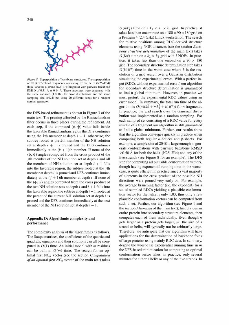
Figure 8. Superposition of backbone structures. The superpositionof 20 RDC-refined fragments consisting of the helix (N25–E34)(blue) and the β-strand (Q2–T7) (magenta) with pairwise backboneRMSD of 0.31 Å ± 0.14 Å. These structures were generated withthe same variance (1.0 Hz) for error distributions and the samesampling size (1024) but using 20 different seeds for a randomnumber generator.

the DFS-based refinement is shown in Figure 3 of themain text. The pruning afforded by the Ramachandranfilter occurs in three places during the refinement. Ateach step, if the computed (φ,ψ) value falls insidethe favorable Ramachandran region the DFS continuesusing the kth member at depth i + 1, otherwise, thesubtree rooted at the kth member of the NH solutionset at depth i + 1 is pruned and the DFS continuesimmediately at the (k + 1)th member. If none of the(φ,ψ) angles computed from the cross product of thej th member of the NH solution set at depth i and allthe members of NH solution set at depth i + 1 fallsinto the favorable region, the subtree rooted at the j thmember at depth i is pruned and DFS continues imme-diately at the (j + 1)th member at depth i. If none ofthe (φ,ψ) angles computed from the cross product ofthe two NH solution sets at depth i and i + 1 falls intothe favorable region the subtree at depth i−1 rooted atthe parent of the current NH solution set at depth i ispruned and the DFS continues immediately at the nextmember of the NH solution set at depth i − 1.

Appendix D: Algorithmic complexity andperformance

The complexity analysis of the algorithm is as follows.The Saupe matrices, the coefficients of the quartic andquadratic equations and their solutions can all be com-puted in O(1) time. An initial model with m residuescan be built in O(m) time. The search for an op-timal first NCα vector (see the section Computationof an optimal first NCα vector of the main text) takes

O(mk31) time on a k1 × k1 × k1 grid. In practice, it

takes less than one minute on a 180×90×180 grid ona Pentium 4 (2.4 GHz) Linux workstation. The searchfor relative positions among RDC-derived structureelements using NOE distances (see the section Back-bone structure determination of the main text) takesO(lk2

2) time on a k2 × k2 grid with l NOEs. In prac-tice, it takes less than one second on a 90 × 180grid. The secondary structure determination step takesO(k16m) time in the worst case where k is the res-olution of a grid search over a Gaussian distributionsimulating the experimental errors. With a perfect in-put (RDCs without experimental errors) our algorithmfor secondary structure determination is guaranteedto find a global minimum. However, in practice wemust perturb the experimental RDC values using anerror model. In summary, the total run time of the al-gorithm is O(n(lk2

2 + mk31 + k16m)) for n fragments.

In practice, the grid search over the Gaussian distri-bution was implemented as a random sampling. Foreach sampled set consisting of a RDC value for everyresidue of a fragment our algorithm is still guaranteedto find a global minimum. Further, our results showthat the algorithm converges quickly in practice whencomputing both regular α-helices and β-sheets. Forexample, a sample size of 2048 is large enough to gen-erate conformations with pairwise backbone RMSD<0.50 Å for both the helix (N25–E34) and any of thefive strands (see Figure 8 for an example). The DFSstep for computing all plausible conformation vectors,though having exponential running time in the worst-case, is quite efficient in practice since a vast majorityof elements in the cross product of the possible NHdirections were pruned very early on. For example,the average branching factor (i.e. the exponent) for aset of sampled RDCs yielding a plausible conforma-tion vector for the helix is only 1.03, thus only a fewplausible conformation vectors can be computed fromsuch a set. Further, our algorithm (see Figure 1 andthe section Algorithm of the main text), first divides anentire protein into secondary structure elements, thencomputes each of them individually. Even though n

gets larger as a protein gets larger, m, the size of astrand or helix, will typically not be arbitrarily large.Therefore, we anticipate that our algorithm will haveapplications for the determination of backbone foldsof large proteins using mainly RDC data. In summary,despite the worst-case exponential running time in m

the DFS-based minimization for computing an optimalconformation vector takes, in practice, only severalminutes for either a helix or any of the five strands. In

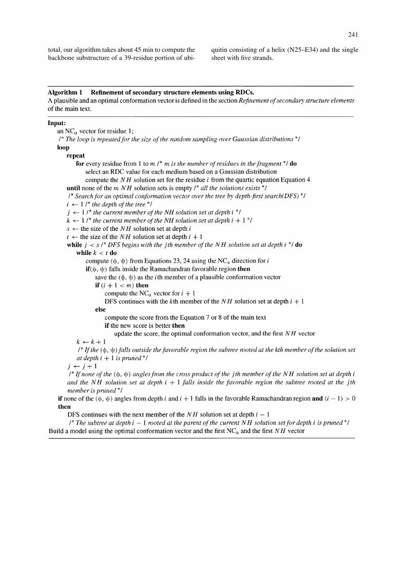
241

total, our algorithm takes about 45 min to compute thebackbone substructure of a 39-residue portion of ubi-

quitin consisting of a helix (N25–E34) and the singlesheet with five strands.

242

References

Al-Hashimi, H.M., Valafar, H., Terrell, M., Zartler, E.R., Eidsness,M.K. and Prestegard, J.H. (2000) J. Magn. Reson., 143, 402–406.

Andrec, M., Du, P. and Levy, R.M. (2001) J. Biomol. NMR, 21,335–347.

Bailey-Kellogg, C., Widge, A., Kelley, J.J., Berardi, M.J., Bush-weller, J.H. and Donald, B.R. (2000) J. Comput. Biol., 7,537–558.

Barbieri, R., Bertini, I., Cavallaro, G., Lee, Y., Luchinat, C. andRosato, A. (2002) J. Am. Chem. Soc., 124, 5581–5587.

Berman, H.M., Westbrook, J., Feng, Z., Gilliland, G., Bhat, T.N.,Weissig, H., Shindyalov, I.N. and Bourne, P.E. (2000) Nucl.Acids Res., 28, 235–242.

Bertram, R., Quine, J.R., Chapman, M.S. and Cross, T.A. (2000) J.Magn. Reson., 147, 9–16.

Brünger, A.T. (1993) XPLOR: A System for X-Ray Crystallographyand NMR, Yale University Press, New Haven.

Chou, J.J., Gaemers, S., Howder, B., Louis, J.M. and Bax, A. (2001)J. Biomol. NMR, 21, 377–382.

Clore, G.M., Gronenborn, A.M. and Bax, A. (1998) J. Magn.Reson., 133, 216–221.

Clore, G.M., Starich, M.R., Bewley, C.A., Cai, M.L. andKuszewski, J. (1999) J. Am. Chem. Soc., 121, 6513–6514.

Cormen, T.H., Leiserson, C.E., Rivest, R.L. and Stein, C. (2001)Introduction to Algorithms, The MIT Press.

Cornilescu, G., Marquardt, J.L., Ottiger, M. and Bax, A. (1998) J.Am. Chem. Soc., 120, 6836–6837.

Delaglio, F., Kontaxis, G. and Bax, A. (2000) J. Am. Chem. Soc.,122, 2142–2143.

Dominguez, C., Boelens, R. and Bonvin, A.M.J.J. (2003) J. Am.Chem. Soc., 125, 1731–1737.

Engh, R.A. and Huber, R. (1991) Acta Cryst., A47, 392–400.Fowler, A.C., Tian, F., Al-Hashimi, H.M. and Prestegard, J.H.

(2000) J. Mol. Biol., 304, 447–460.Gardner, K.H. and Kay, L.E. (1997) J. Am. Chem. Soc., 119, 7599–

7600.Giesen, A.W., Homans, S.W. and Brown, J.M. (2003) J. Biomol.

NMR 25, 63–71.Gnu (2002) The gnu general public license, http://

www.gnu.org/licenses/licenses.htmlGüntert, P., Mumenthaler, C. and Wüthrich, K. (1997) J. Mol. Biol.,

273, 283–298.

Hansen, M.R., Hanson, P. and Pardi, A. (2000) Meth. Enzymol.,317, 220–240.

Hus, J.C., Marion, D. and Blackledge, M. (2001) J. Am. Chem. Soc.,123, 1541–1542.

Kac, M. (1948) Proc. London Math. Soc., 50, 390–408.Kemple, M.D., D., R.B., Lipkowitz, K.B., Prendergast, F.G. and

Rao, B.D. (1988) J. Am. Chem. Soc., 110, 8275– 8287.Kolinski, A. and Skolnick, J. (1998) Proteins, 32, 475–494.Losonczi, J.A., Andrec, M., Fischer, M.W. and Prestegard, J.H.

(1999) J. Magn. Reson., 138, 334–342.Meiler, J., Blomberg, N., Nilges, M. and Griesinger, C. (2000) J.

Biomol. NMR, 16, 245–252.Nomura, K. and Kainosho, M. (2002) J. Magn. Reson., 154, 146–

153.Ottiger, M. and Bax, A. (1998) J. Am. Chem. Soc., 120, 12334–

12341.Quine, J.R., Brenneman, M. and Cross, T. (1997) Biophys. J., 72,

2342–2348.Ramirez, B.E. and Bax, A. (1998) J. Am. Chem. Soc., 120, 9106–

9107.Rienstra, C.M., Tucker-Kellogg, L., Jaroniec, C.P., Hohwy, M.,

Reif, B., McMahon, M.T., Tidor, B., Lozano-Pèrez, T. andGriffin, R.G. (2002) Proc. Natl. Acad. Sci. USA, 99, 10260–10265.

Rohl, C.A. and Baker, D. (2002) J. Am. Chem. Soc., 124, 2723–2729.

Saupe, A. (1968) Angew. Chem., 7, 97–112.Stryer, L. (1994) Biochemistry, W.H. Freeman and Company.Tian, F., Valafar, H. and Prestegard, J.H. (2001) J. Am. Chem. Soc.,

123, 11791–11796.Tjandra, N. and Bax, A. (1997) Science, 278, 1111–1114.Tolman, J.R., Flanagan, J.M., Kennedy, M.A. and Prestegard, J.H.

(1995) Proc. Natl. Acad. Sci. USA, 92, 9279–9283.Vijay-Kumar, S., Bugg, C.E. and Cook, W.J. (1987) J. Mol. Biol.,

194, 531–544.Wang, L., Pang, Y., Holder, T., Brender, J., Kurochkin, A.V. and

Zuiderweg, E.R.P. (2001) Proc. Natl. Acad. Sci. USA, 98, 7684–7689.

Wang, Y.X., Marquardt, J.L., Wingfield, P., Stahl, S.J., Lee-Huang,S., Torchia, D. and Bax, A. (1998) J. Am. Chem. Soc., 120, 7385–7386.

Wedemeyer, W.J., Rohl, C.A. and Scheraga, H.A. (2002) J. Biomol.NMR, 22, 137–151.

Yue, K. and Dill, K.A. (2000) Protein Sci., 9, 1935–1946.