CASE BASED STUDY TO ANALYZE THE APPLICABILITY OF LINEAR & NONLINEAR MODELS

David C. Wyld et al. (Eds) : COSIT, DMIN, SIGL, CYBI, NMCT, AIAPP - 2014 pp. 09–19, 2014. © CS & IT-CSCP 2014 DOI : 10.5121/csit.2014.4902

CASE BASED STUDY TO ANALYZE THE

APPLICABILITY OF LINEAR & NON-

LINEAR MODELS

Anubhav Gupta1, Gaurav Singh Thakur2 , Ankur Bhardwaj3 and

Biju R Mohan4

Department of Information Technology,

National Institute of Technology Karnataka, Surathkal [email protected]

[email protected] [email protected]

[email protected]

ABSTRACT

This paper uses a case based study – “product sales estimation” on real-time data to

understand the applicability of linear and non-linear models. We use a systematic approach to

address the given problem statement of sales estimation for a given product by applying both

linear and non-linear techniques on a data set of selected features from the original data set.

Feature selection is a process that reduces the dimensionality of the data set by eliminating

those features which contribute minimal to the prediction of the dependent variable. The next

step is training the model which is done using two techniques from linear & non-linear

domains, one of the best ones in their respective areas. Data Re-modeling has then been done to

extract new features from the data set by changing the structure of the dataset & the

performance of the models is checked again. Data Remodeling often plays a crucial role in

boosting classifier accuracies by changing the properties of the dataset. We then try to analyze

the reasons due to which one model proves to be better than the other & hence try and develop

an understanding about the applicability of linear & non-linear models. The target mentioned

above being our primary goal, we also aim to find the classifier with the best possible accuracy

for product sales estimation in the given scenario.

KEYWORDS

Machine Learning, Prediction, Linear and Non-linear models, Linear Regression, Random

Forest, Dimensionality Reduction, Feature Selection, Homoscedasticity.

1. INTRODUCTION

Machine learning is a branch of artificial intelligence. It concerns the construction and study of systems that can learn from data. For example, a machine learning algorithm can be used to classify people by gender, by data such as height, Body Mass Index, Favorite color etc. There are various types of Machine Learning Algorithm; two of the main types are Supervised Learning

10 Computer Science & Information Technology (CS & IT)

(where the desired output is Known), and Unsupervised Learning (where the desired output is not known). In this paper, we discuss the techniques which belong to Supervised learning[3]. Predicting the future sales of a new product in the market has intrigued many scholars and industry leaders as a difficult and challenging problem. It involves customer sciences and helps the company by analyzing data and applying insights from a large number of customers across the globe to predict the sales in the upcoming time in near future. The success or failure of a new product launch is often evident within the first few weeks of sales. Therefore, it is possible to forecast the sales of the product in the near future by analyzing its sales in the first few weeks. We propose to predict the success or failure of each of product launches 26 weeks after the launch, by estimating their sales in the 26th week based only on information up to the 13th week after launch. We intend to do so by combining data analysis with machine learning techniques and use the results for forecasting. We have used the divided the work into following phases:

i) Dimensionality reduction (Feature selection)

ii) Application of Linear & Non-Linear Learning Models

iii) Data Re-modeling

iv) Re-application of learning models.

v) Evaluation of the performance of the learning models through comparative study &

Normality tests.

vi) Boosting the accuracy of the model that better suits the problem based on their evaluation.

To create a forecasting system for this problem statement we gathered 26 weeks information for nearly 2000 Products belonging to 198 categories to train our model. Various attributes such as units_sold_that_week, Stores_selling_in_the_nth_week, Cumulative units sold to a number of different customer groups etc are used as independent variables to train & predict the dependent variable- “Sales_in_the_nth_week”. However our task here is only to predict their sales in the 26th week. In Section 2, we discuss about the methodology and work done in each of the phases, followed by the results & discussion in Section 3. Finally we draw a conclusion in Section 4 along with its applications, followed by the references.

2. METHODOLOGY AND WORK DONE

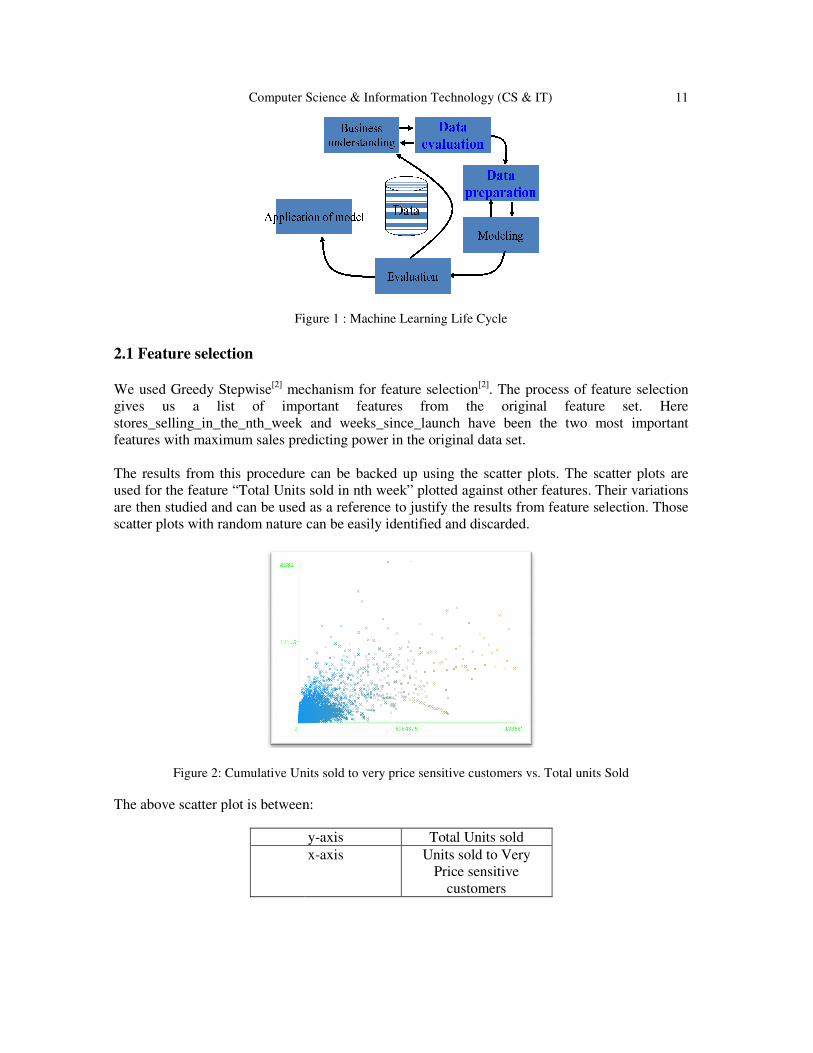
A basic block diagram to explain the entire process of Machine Learning is given below.

Computer Science &

Figure

2.1 Feature selection

We used Greedy Stepwise[2] mechanism for feature selectiongives us a list of important featurestores_selling_in_the_nth_week features with maximum sales predicting power The results from this procedure can be backed up using the scatter plots. The scatter plots are used for the feature “Total Units soldare then studied and can be used as a reference scatter plots with random nature can be easily identified and discarded.

Figure 2: Cumulative Units sold to very price sensitive customers The above scatter plot is between:

Computer Science & Information Technology (CS & IT)

Figure 1 : Machine Learning Life Cycle

mechanism for feature selection[2]. The process of feature selectionus a list of important features from the original feature set. Here

and weeks_since_launch have been the two most important predicting power in the original data set.

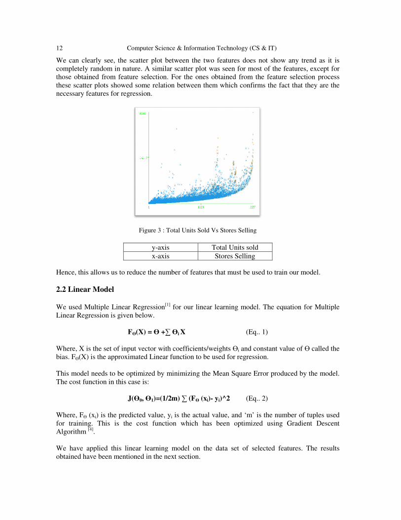
The results from this procedure can be backed up using the scatter plots. The scatter plots are used for the feature “Total Units sold in nth week” plotted against other features. Their

used as a reference to justify the results from feature selectionscatter plots with random nature can be easily identified and discarded.

: Cumulative Units sold to very price sensitive customers vs. Total units Sold

The above scatter plot is between:

y-axis Total Units sold x-axis Units sold to Very

Price sensitive customers

11

process of feature selection the original feature set. Here

the two most important

The results from this procedure can be backed up using the scatter plots. The scatter plots are nst other features. Their variations

to justify the results from feature selection. Those

Total units Sold


We can clearly see, the scatter plot between the two featurescompletely random in nature. A those obtained from feature selectionthese scatter plots showed some relation between themnecessary features for regression.

Figure 3 : Total Units Sold Vs Stores Selling

Hence, this allows us to reduce the number of features that must be used to train our model. 2.2 Linear Model

We used Multiple Linear RegressionLinear Regression is given below.

FӨ(X) =

Where, X is the set of input vector with coefficients/weights bias. FӨ(X) is the approximated Linear function to be used for regression. This model needs to be optimized by minimizing the Mean Square The cost function in this case is:

J(Ө0, Ө

Where, FӨ (xi) is the predicted value, yfor training. This is the cost function which has been optimized Algorithm [4]. We have applied this linear learning model on the data set of selected features. The results obtained have been mentioned in the next section.

Computer Science & Information Technology (CS & IT)

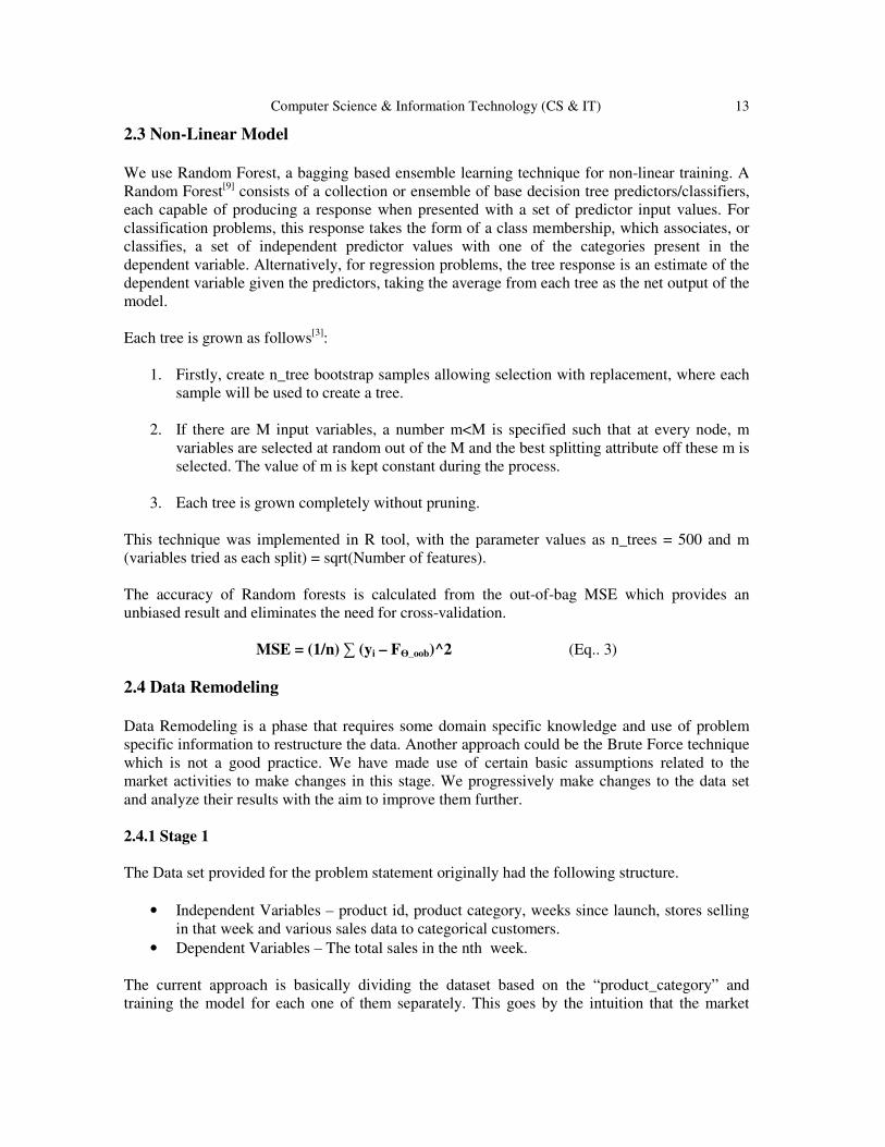
e can clearly see, the scatter plot between the two features does not show any trend as it is similar scatter plot was seen for most of the features, except f

those obtained from feature selection. For the ones obtained from the feature selection processsome relation between them which confirms the fact that they are the

necessary features for regression.

Figure 3 : Total Units Sold Vs Stores Selling

y-axis Total Units sold x-axis Stores Selling

Hence, this allows us to reduce the number of features that must be used to train our model.

used Multiple Linear Regression[1] for our linear learning model. The equation for Multiple Linear Regression is given below.

(X) = Ө +∑ Өi X (Eq.. 1)

Where, X is the set of input vector with coefficients/weights Өi and constant value of (X) is the approximated Linear function to be used for regression.

This model needs to be optimized by minimizing the Mean Square Error produced by the model.

Ө1)=(1/2m) ∑ (FӨ (xi)- yi)^2 (Eq.. 2)

) is the predicted value, yi is the actual value, and ‘m’ is the number of tupfor training. This is the cost function which has been optimized using Gradient Descent

We have applied this linear learning model on the data set of selected features. The results have been mentioned in the next section.

does not show any trend as it is similar scatter plot was seen for most of the features, except for

obtained from the feature selection process which confirms the fact that they are the

Hence, this allows us to reduce the number of features that must be used to train our model.

The equation for Multiple

and constant value of Ө called the

Error produced by the model.

e, and ‘m’ is the number of tuples used using Gradient Descent

We have applied this linear learning model on the data set of selected features. The results

Computer Science & Information Technology (CS & IT) 13

2.3 Non-Linear Model

We use Random Forest, a bagging based ensemble learning technique for non-linear training. A Random Forest[9] consists of a collection or ensemble of base decision tree predictors/classifiers, each capable of producing a response when presented with a set of predictor input values. For classification problems, this response takes the form of a class membership, which associates, or classifies, a set of independent predictor values with one of the categories present in the dependent variable. Alternatively, for regression problems, the tree response is an estimate of the dependent variable given the predictors, taking the average from each tree as the net output of the model. Each tree is grown as follows[3]:

1. Firstly, create n_tree bootstrap samples allowing selection with replacement, where each sample will be used to create a tree.

2. If there are M input variables, a number m<M is specified such that at every node, m

variables are selected at random out of the M and the best splitting attribute off these m is selected. The value of m is kept constant during the process.

3. Each tree is grown completely without pruning.

This technique was implemented in R tool, with the parameter values as n_trees = 500 and m (variables tried as each split) = sqrt(Number of features). The accuracy of Random forests is calculated from the out-of-bag MSE which provides an unbiased result and eliminates the need for cross-validation.

MSE = (1/n) ∑ (yi – FӨ_oob)^2 (Eq.. 3)

2.4 Data Remodeling

Data Remodeling is a phase that requires some domain specific knowledge and use of problem specific information to restructure the data. Another approach could be the Brute Force technique which is not a good practice. We have made use of certain basic assumptions related to the market activities to make changes in this stage. We progressively make changes to the data set and analyze their results with the aim to improve them further. 2.4.1 Stage 1 The Data set provided for the problem statement originally had the following structure.

• Independent Variables – product id, product category, weeks since launch, stores selling in that week and various sales data to categorical customers.

• Dependent Variables – The total sales in the nth week. The current approach is basically dividing the dataset based on the “product_category” and training the model for each one of them separately. This goes by the intuition that the market


sales patterns and demands-supply varies differently for different categories. And hence we regress separately for each category and use that model to predict the sales of a product for the 26th week. After some study, we had already identified in the initial phase that, for a particular category of product, only the weeks since launch and number of stores selling have a major effect in predicting the total sales for that week. But this model was not exactly suitable as:

• Firstly, the sales in the 26th week apart from stores selling are also dependent on the sales in the previous weeks which were not being considered in the previous data model.

• Secondly, since in the test cases, the data provided is only for 13 weeks, the training must also not include any consumer specific sales data from beyond 13 weeks.

• The independent variable to be predicted must be the “Total Sales in the 26th week” and not the “Total Sales in the nth week”.

Hence, we have modified the data set such that we use the sales in every week upto 13 weeks along with the stores selling in week 26 as a feature set to estimate the sales in week 26. This way we can also measure the predictive power of sales in each week and how do they affect the sales in the later stages. This has been analyzed using feature selection on the new set and also through performing an Autocorrelation analysis on the ‘sales_in_nth_week’ to find the correlation between the sales series with itself for a given lag. The acf value for lag 1 was 0.8 and for lag 2 was 0.6 showing that with so much persistence, there is a lot of predictive power in the Total sales in a given week that can help us predict the sales for atleast two more weeks. Finally, the new structure of the dataset for this problem statement is as follows:

• Independent Variables – Sales in week1, Sales in week2, Sales in week3… Sales in week13, stores_selling_in_the_13th_week

• Dependent variable - Total Sales in the 26th week. This dataset was then subjected to both Linear & Non-linear learning models. The one which performs better would then be used to train on the next phase of Data Remodeling. 2.4.2 Stage 2

We needed to further modify the data structure to improve results and also find a method by which we could regress the data set for all the categories together. This meant trying to find a model that allowed us to train a single model that could work on all the categories together. To do this, we used the following strategy:

1. Let ‘usn’ represent Units_sold_in_week_n and ‘ssn’ represent Stores_selling_in_week_n.

2. Now, as we had previously obtained the hypothesis from Linear Regression (Eq.. 1), in the form of:

usn = (k) x ssn (Eq.. 4)


where k is the co-efficient of ssn. Note that k is the only factor which would vary from category to category.

3. Therefore, from Eq.. 4, we get 1. us26 = (k) x ss26 (Eq.. 5) 2. us13 = (k) x ss13 (Eq.. 6) 3. => us26/ us13 = ss26/ ss13 (Eq.. 7) 4. => us26= ss26/ ss13 * us13 (Eq.. 8)

4. In this way, we remove the need for finding the need of the Coefficient of ssn for each

category and simply keep an additional attribute ‘ss26/ ss13 * us13’.

5. Also, instead of keeping only the “Stores_selling” in week 26, we decided to keep

“Stores_selling” from week 14 to 26 to further incorporate the trend (if any) of the Stores_selling against Units_sold_in_week_26. This was the only useful feature provided beyond 13th week. The number of stores could help us identify the trends in the sales of the product hence further improving the accuracy of our predictions in the 26th week.

Hence the structure of our new dataset was as follows:

1. For each of weeks 1 to 13, the ratio of stores in week 26 to stores in week 13, multiplied by the sales in that week.

2. The raw sales in weeks 1 through 13 3. The number of stores in weeks 14 through 26.

The results obtained from these changes are explained later in the next section. 2.5 Understanding the Applicability of Models

Any Linear model can only be applied on a given dataset assuming that it encompasses the following properties, else it performs poorly.

1. Linearity of the relationship between dependent and independent variables. 2. Independence of the errors (no serial correlation). 3. Homoscedasticity

[12] means that the residuals are not related to the variable plotted on X-

axis. 4. Normality of the error distribution.

In this case we test these properties to understand and justify the performance of Linear Models against a Non-Linear Models in this domain. These tests are conducted by:

1. Linear relationship among the features is a domain based question. For example does the “sales to price sensitive customer” affect its “stores selling in nth week”. Such errors can be fixed only by applying transformations that take into account the interactions between the features.


2. Independence of errors is tested by plotting the Autocorrelation graph for the residuals. Serial correlation in the residuals implies scope for improvement and extreme serial correlation is a symptom of a bad model.

3. If the variance of the errors increases with time, confidence intervals for out of-sample

predictions tend to be unrealistically narrow. To test this we look at plots of residuals

versus time and residuals versus predicted value, and look for residuals that increase (i.e., more spread-out) either as a function of time or the predicted value.

4. The best test for normally distributed errors is a normal probability plot of the residuals. This is a plot of the fractiles of error distribution versus the fractiles of a normal distribution having the same mean and variance. If the distribution is normal, the points on this plot fall close to the diagonal line.

The results obtained in these tests are given in the next section.

3. RESULTS AND DISCUSSION

3.1 Feature selection

The list of features obtained from Greedy Stepwise feature selection[2] showed that “Stores Selling in nth week” and “weeks since launch” were the most important features contributing to the prediction of sales. The variance of these features with the dependent variable, together is greater than 0.94 showing that they contribute the maximum to the prediction of sales.

3.2 Application of Linear Regression And Random Forest

Linear Regression Considering the top 6 features obtained from feature selection procedure based on their variances:

Correlation Coefficient 0.9339 Mean Absolute Error 28.37 RMSE 69.9397

Random Forests considering all the features:

OOB-RMSE 46.26 As we currently see, the non-linear model is working better than the linear model. This may lead to a jumpy conclusion that non-linear model is probably better in this scenario. Moreover the accuracy of the classifiers is also not great due to the high RMSE values of both the models.

3.3 Application of Learning Models after Data Re-modeling Phase-1

Linear Regression Results:



Random Forest Results:

OOB-RMSE 7.19 As we see here, the performance of both the models have improved drastically, however, we find that the linear model outperforms random forest. This finding compelled us to inquire about the properties of the dataset that satisfied the assumptions of the linear model. We found that:

i) The Franke’s Anscombe[11] experiment to test the normality of data distribution came out inconclusive leading us to use the Normal Q-Q plot[13].

ii) The Normal Q-Q plot in R[14] concluded that the dataset follows the normal distribution.

iii) The residuals also follow the normal distribution curve under the Normal Q-Q plot just like the actual data conforming the second assumption of linearity.

iv) We check the Homoscedasticity[12] property by plotting the residuals against fitted values. The graph was completely random in nature.

v) Lastly, the linear relationship between features is a domain specific question. The data collected mostly contains the sales data from local stores, from local manufactures of items of daily consumption types like – bread, milk_packets, airbags, etc. Since these types of products belong to a class of items where the stochastic component is negligible, it makes it easy for us to assume that the linear model can be easily applied to this problem. This is the reason why linear model is working better compared to the non-linear model due to negligible interaction of the features.

3.4 Application of Linear Models after Data Re-modeling Phase-2

Linear Regression Results considering all the new features:


Linear Regression Results considering only top 6 new features after applying feature selection on the new dataset:


As we see, the results have improved further, with the accuracy of the classifier going up from RMSE value of approximately 65 to 0.43. With the final model, we were able to predict the Total


sales of any given product in the test set with an error < 1 unit for any category, our best RMSE achieved being 0.43.

4. CONCLUSION

The primary target in machine learning is to produce the best learning models which can provide accurate results that assist in decision making, forecasting, etc. This brings us to the essential question of finding the best suitable model that can be applied to any given problem statement. We have performed a case based study here to understand on how to decide whether a linear or a non-linear model is best suited for a given application. We initially follow a basic approach by adopting two leading classifiers from each domain and evaluate their performances. We then try to boost the accuracies of both the learning models using data re-structuring. The results obtained from this process help us derive an important empirical proof that the accuracy of a classifier not just depends on its algorithm. There is no such certainty that a more complex algorithm will perform better than a simple one. As we see in this case, Random Forests, which belong to the class of ensemble classifiers bagging based is known to perform well and produce high accuracies. However, here the simple Multiple Linear Regression model outperforms the previous one. The accuracy of the model largely depends on the problem domain where it is being applied and the data set, as the domain decides the properties that the data set would inherit and this greatly determines the applicability of any machine learning technique. Hence holding a prejudice for/against any algorithm may not provide optimal results in machine learning. To further this observation, the use of various other algorithms such as Artificial Neural Networks (Which is known to give great results in case both Linear and Non-linear Machine learning problems), as well as Support Vector Machines (Which are known to give very high accuracies) are suggested. The framework developed here has been tested on real-time data and has provided accurate results. This framework can be used for the forecasting of daily use products, items of everyday consumption, etc. from local manufacturers, as it follows the assumption that the features have minimum interaction with each other. Branded products from big manufacturers include many more market variables, like the effect of political and economic factors, business policies, government policies, etc. which increase the stochastic factor in the product sales & also increase the interaction among the independent features. This feature interaction is very minimal for local products. Extending this framework to the “branded” scenario will require significant changes. However, the current model is well suited to small scale local products and can be easily used with minimal modifications, for accurate predictions. REFERENCES

[1] Jacky Baltes, Machine Learning Linear Regression , University of Manitoba , Canada [2] Isabelle Guyon and Andrẻ Elisseeff ,An Introduction to Variable and Feature Selection, Journal of

Machine Learning Research 3 (2003) 1157-1182 [3] Jiawei Han and Micheline Kamber, Data Mining –Conepts and Techniques , Second Edition Page-79-

80 [4] Kris Hauser , Document B553, Gradient Descent, January 24,2012


[5] Luis Carlos Molina, Lluís Belanche, Àngela Nebot ,Feature Selection Algorithms: A Survey and Experimental Evaluation, University Politècnica de Catalunya

[6] Quang Nhat Nyugen, Machine Learning Algorithms and applications, University of Bozen-Bolzano, 2008-2009

[7] Jan Ivar Larsen, Predicting Stock Prices Using Technical Analysis and Machine Learning, Norwegian University of Science and Technology

[8] Classification And Regression By Random Forest by Andy Liaw And Matthew Wiener, Vol 2/3, December 2002

[9] Lecture 22,Classification And Regression Trees, 36-350, http://www.stat.cmu.edu/, November 2009 [10] [Online] Anscombe’s Quartet- http://en.wikipedia.org/wiki/Anscombe's_quartet [11] [Online] Homoscedasticity- http://en.wikipedia.org/wiki/Homoscedasticity [12] [Online] Normal Q-Q Plot- http://en.wikipedia.org/wiki/Q–Q_plot [13] [Online] Quick R-http://www.statmethods.net/advgraphs/probability.html

AUTHORS

Biju R Mohan He is an Assistant Professor at National Institute of Technology Karnataka, Surathkal in the department of Information Technology. His areas of interest are Software Aging, Virtualization, Software Engineering, Software Architecture, Software Patterns, Requirements Engineering.

Gaurav Singh Thakur

Gaurav Singh Thakur completed his B.Tech in Information Technology from National Institute of Technology Surathkal and is currently working as a Software Engineer at Cisco Systems, Inc. Bangalore. His technical areas of interest include Machine learning, Networking & Security and Algorithms. Anubhav Gupta

Anubhav completed his Bachelors , in National Institute of Technology Karnataka, Surathkal in the Field of Information Technology (IT). His areas of interest are Machine learning, Information Security, Web Development and Algorithms. He is currently working as Software Developer Engineer at Commonfloor (MaxHeap Technologies). Ankur Bhardwaj

He has pursued his B.Tech. in Information Technology from National Institute of Technology Karnataka, Surathkal. His areas of interest are Machine Learning, Statistics and Algorithms. He is currently working as Associate Professional at Computer Sciences Corporation.

CASE BASED STUDY TO ANALYZE THE APPLICABILITY OF LINEAR & NONLINEAR MODELS

Documents

Transcript of CASE BASED STUDY TO ANALYZE THE APPLICABILITY OF LINEAR & NONLINEAR MODELS