Variable Selection and Model Averaging in Semiparametric Overdispersed Generalized Linear Models
35
arXiv:0707.2158v1 [stat.ME] 14 Jul 2007 VARIABLE SELECTION AND MODEL AVERAGING IN SEMIPARAMETRIC OVERDISPERSED GENERALIZED LINEAR MODELS REMY COTTET, ROBERT KOHN, AND DAVID NOTT Summary Flexibly modeling the response variance in regression is important for efficient param- eter estimation, correct inference, and for understanding the sources of variability in the response. Our article considers flexibly modelling the mean and variance functions within the framework of double exponential regression models, a class of overdispersed generalized linear models. The most general form of our model describes the mean and dispersion parameters in terms of additive functions of the predictors. Each of the additive terms can be either null, linear, or a fully flexible smooth effect. When the dispersion model is null the mean model is linear in the predictors and we obtain a generalized linear model, whereas with a null dispersion model and fully flexible smooth terms in the mean model we obtain a generalized additive model. Whether or not to include predictors, whether or not to model their effects linearly or flexibly, and whether or not to model overdispersion at all is determined from the data using a fully Bayesian approach to inference and model selection. Model selection is ac- complished using a hierarchical prior which has many computational and inferential advantages over priors used in previous empirical Bayes approaches to similar prob- lems. We describe an efficient Markov chain Monte Carlo sampling scheme and priors that make the estimation of the model practical with a large number of predictors. The methodology is illustrated using real and simulated data. Key Words: Bayesian analysis; Double exponential family; Hierarchical priors; Vari- ance estimation. 1. Introduction Flexibly modelling the response variance in regression is important for efficient estimation of mean parameters, correct inference and for understanding the sources of variability in the response. Re- sponse distributions that are commonly used for modelling non-Gaussian data such as the binomial 1
-
Upload
independent -
Category
Documents
-
view
5 -
download
0
Transcript of Variable Selection and Model Averaging in Semiparametric Overdispersed Generalized Linear Models

arX
iv:0
707.
2158
v1 [
stat
.ME
] 1
4 Ju
l 200
7
VARIABLE SELECTION AND MODEL AVERAGING IN SEMIPARAMETRIC
OVERDISPERSED GENERALIZED LINEAR MODELS
REMY COTTET, ROBERT KOHN, AND DAVID NOTT
Summary
Flexibly modeling the response variance in regression is important for efficient param-
eter estimation, correct inference, and for understanding the sources of variability in
the response. Our article considers flexibly modelling the mean and variance functions
within the framework of double exponential regression models, a class of overdispersed
generalized linear models. The most general form of our model describes the mean
and dispersion parameters in terms of additive functions of the predictors. Each of
the additive terms can be either null, linear, or a fully flexible smooth effect. When
the dispersion model is null the mean model is linear in the predictors and we obtain
a generalized linear model, whereas with a null dispersion model and fully flexible
smooth terms in the mean model we obtain a generalized additive model. Whether
or not to include predictors, whether or not to model their effects linearly or flexibly,
and whether or not to model overdispersion at all is determined from the data using
a fully Bayesian approach to inference and model selection. Model selection is ac-
complished using a hierarchical prior which has many computational and inferential
advantages over priors used in previous empirical Bayes approaches to similar prob-
lems. We describe an efficient Markov chain Monte Carlo sampling scheme and priors
that make the estimation of the model practical with a large number of predictors.
The methodology is illustrated using real and simulated data.
Key Words: Bayesian analysis; Double exponential family; Hierarchical priors; Vari-
ance estimation.
1. Introduction
Flexibly modelling the response variance in regression is important for efficient estimation of mean
parameters, correct inference and for understanding the sources of variability in the response. Re-
sponse distributions that are commonly used for modelling non-Gaussian data such as the binomial1

2 REMY COTTET, ROBERT KOHN, AND DAVID NOTT
and Poisson, although natural and interpretable, have a variance that is a function of the mean and
often real data exhibits more variability than might be implied by the mean-variance relationship, a
phenomenon referred to as overdispersion. Underdispersion, where the data exhibits less variability
than expected, can also occur, although this is less frequent.
Generalized linear models (GLMs) have traditionally been used to model non-Gaussian regression
data (Nelder and Wedderburn, 1972 , McCullagh and Nelder, 1989), where the response y has a
distribution from the exponential family and a transformation of the mean response is a linear function
of predictors. This framework is extended to generalized additive models (GAMs) by Hastie and
Tibshirani (1990) where a transformation of the mean is modelled as a flexible additive function of
the predictors. However, the restriction to the exponential family in GLMs and GAMs is sometimes
not general enough. While there is often strong motivation for using exponential family distributions
on the grounds of interpretability, the variance of these distributions is a function of the mean and
the data often exhibit greater variability than is implied by such mean-variance relationships.
Quasi-likelihood (Wedderburn, 1974) provides one simple approach to inference in the presence of
overdispersion, where the exponential family assumption is dropped and only a model for the mean is
given with the response variance a function of the mean up to a multiplicative constant. However, this
approach does not allow overdispersion to be modelled as a function of covariates. An extension of
quasi-likelihood which allows this is the extended quasi-likelihood of Nelder and Pregibon (1987), but
in general extended quasi-likelihood estimators may not be consistent (Davidian and Carroll, 1988).
Use of a working normal likelihood for estimating mean and variance parameters can also be used
for modelling overdispersion (Peck et al., 1984). However, the non-robustness of the estimation of
mean parameters when the variance function is incorrectly specified is a difficulty with this approach.
Alternatively, a generalized least squares estimating equation for mean parameters can be combined
with a normal score estimating equation for variance parameters, a procedure referred to as pseudo-
likelihood (Davidian and Carroll, 1987). Both the working normal likelihood and pseudolikelihood
approaches are related to the theory of generalized estimating equations (see Davidian and Giltinan,
1995, p. 57). Additive extensions of generalized estimating equations are considered by Wild and
Yee (1996). Smyth (1989) considers modelling the mean and variance in a parametric class of models
which allows normal, inverse Gaussian and gamma response distributions, and a quasi-likelihood ex-
tension is also proposed which uses a similar approach to pseudolikelihood for estimation of variance
parameters. Smyth and Verbyla (1999) consider extensions of residual maximum likelihood (REML)
estimation of variance parameters to double generalized linear models where dispersion parameters
are modelled linearly in terms of covariates after transformation by a link function.

OVERDISPERSED MODELS 3
Inference about mean and variance functions using estimating equations has the drawback that there
is no fully specified model, making it difficult to deal with characteristics of the predictive distribution
for a future response, other than its mean and variance. Model based approaches to modelling overdis-
persion include exponential dispersion models and related approaches (Jorgensen, 1997 , Smyth, 1989),
the extended Poisson process models of Faddy (1997) and mixture models such as the beta-binomial,
negative binomial and generalized linear mixed models (Breslow and Clayton, 1993, Lee and Nelder,
1996) . One drawback of mixture models is that they are unable to model underdispersion. Gen-
eralized additive mixed models incorporating random effects in GAMs are considered by Lin and
Zhang (1999) . Both Yee and Wild (1996) and Rigby and Stasinopoulos (2005) consider very general
frameworks for additive modelling and algorithms for estimating the additive terms. There is clearly
scope for further research on inference: Rigby and Stasinopoulos (2005) suggest that one use for their
methods is as an exploratory tool for a subsequent fully Bayesian analysis of the kind considered in
our article. See also Brezger and Lang (2005) and Smith and Kohn (1996) for other recent work on
Bayesian generalized additive models.
Our framework for flexibly modelling the mean and variance functions is based on the double ex-
ponential regression models introduced by Efron (1986), an approach which is also related to the
extended quasi-likelihood of Nelder and Pregibon (1987). The double exponential family has been
further extended by Gelfand and Dalal (1990) and Gelfand et al. (1997). Double exponential re-
gression models do not suffer the drawbacks of extended quasi-likelihood which occur because the
extended quasi-likelihood is not a proper log likelihood function. Semiparametric double exponen-
tial regression models can be used to extend both generalized linear models and generalized additive
models and are able to model both overdispersion and underdispersion. They provide a convenient
framework for modelling as they have the parsimony and interpretability of GLMs, while allowing, if
necessary, the flexible dependence of the link transformed mean and variance parameters on predic-
tors. The most general model considered in our article describes the mean and dispersion parameters
after transformation by link functions as additive functions of the predictors. For each of the additive
terms in the mean and dispersion models we are able to choose between no effect, a linear effect or
a fully flexible effect. For a null dispersion model and linear effects in the mean model we obtain
generalized linear models, while for a null dispersion model and flexible effects in the mean model we
obtain generalized additive models. The main contribution of the paper is to describe a fully Bayesian
approach to inference that allows the data to decide whether or not to include predictors, whether or
not to model the effect of predictors flexibly or linearly, and whether or not to model overdispersion

4 REMY COTTET, ROBERT KOHN, AND DAVID NOTT
at all. We note that an important benefit of variable selection and model averaging is that it pro-
duces more efficient model estimates when there are redundant covariates or parameters. As far as
we know, alternative approaches to flexible modelling of a mean and variance function do not address
similar issues of model selection in a systematic way that is practically feasible when there are many
predictors. Nott (2004) considers Bayesian nonparametric estimation of a double exponential family
model. However Nott’s paper does not consider model averaging, and his priors for the unknown
functions and smoothing parameters are very different from those used by our article.
Our article refines and generalizes the work of Shively et al. (1999) and Yau, Kohn and Wood (2003)
on nonparametric variable selection and model averaging in probit regression models. These papers
use a data-based prior to carry out variable selection. To construct this prior it is necessary to first
estimate the model with all flexible terms included, even though the actual fitted model may require
only a much smaller number of such terms. This makes the approach impractical when there are a
moderate to large number of terms in the full model because the Markov chain simulation breaks
down. See Yau et al. (2003), who discuss this problem and also give some strategies to overcome it.
Another contribution of our article is to overcome the problems with the data-based prior approach
by specifying hierarchical priors for the linear terms and flexible terms in both the mean and variance
models. The hierarchical specification in our article is also computationally more efficient than the
data-based prior approach because it requires one simulation run through the data, whereas the data-
based approach requires two runs, the first to obtain the data-based prior and the second to estimate
the parameters of the model. Our approach also applies to variable selection and model averaging
in generalized linear models and overdispersed generalized linear models where some or all of the
predictors enter the model parametrically. A third contribution of the paper is to develop an efficient
Markov chain Monte Carlo (MCMC) sampling scheme for carrying out the computations required for
inference in the model.
The paper is organized as follows. Section 2 describes the model, priors and our Bayesian approach
to inference and model selection. Section 3 discusses an efficient Markov chain Monte Carlo sampling
scheme for carrying out the calculations required for inference. Section 4 applies the methodology to
both real and simulated data sets. Section 5 reviews and concludes the paper.

OVERDISPERSED MODELS 5
2. Model and prior distributions
2.1. The double exponential family. Write the density of a random variable y from a one param-
eter exponential family as
(2.1) p(y;µ, φ/A) = exp
(
yψ − b(ψ)
φ/A+ c(y,
φ
A)
)
,
where ψ is a location parameter, φ/A is a known scale parameter and b(·) and c(·, ·) are known
functions. The mean of y is µ = b′(ψ) and the variance of y is (φ/A) b′′(ψ). This means that
ψ = ψ(µ) is a function of µ and so is the variance. Examples of densities which can be written in
this form are the Gaussian, binomial, Poisson and gamma (McCullagh and Nelder, 1989). In (2.1) we
write the scale parameter as φ/A in anticipation of later discussion of regression models where φ is
common to all responses but A may vary between responses. A double exponential family is defined
from a corresponding one parameter exponential family by
(2.2) p(y;µ, θ, φ/A) = Z(µ, θ, φ/A)θ1/2p(y;µ, φ/A)θp(y; y, φ/A)1−θ ,
where θ is an additional parameter and Z(µ, θ, φ/A) is a normalizing constant. To get some intuition
for this definition consider a Gaussian density with variance 1, and apply the double exponential
family construction: the resulting double Gaussian distribution is in fact an ordinary Gaussian den-
sity with mean µ and variance 1/θ so that we can think of the parameter θ as a scale parameter
modelling overdispersion (θ < 1) or underdispersion (θ > 1) with respect to the original one param-
eter exponential family density. While the double Gaussian density is simply the ordinary Gaussian
density, for distributions like the binomial and Poisson, where the variance is a function of the mean,
the corresponding double binomial and double Poisson densities are genuine extensions which allow
modelling of the variance. Efron (1986) shows that
(2.3) E(y) ≈ µ, V ar(y) ≈φ
Aθb′′(ψ), and Z(µ, θ, φ/A) ≈ 1
with these expression being exact for θ = 1. Equation (2.3) helps to interpret the parameters in the
double exponential model and shows how the GLM mean variance relationship is embedded within the
double exponential family, which is important for parsimonious modelling of the variance in regression.
2.2. Semiparametric double exponential regression models. Efron (1986) considers regression
models with a response distribution from a double exponential family, such that both the mean
parameter µ and the dispersion parameter θ are functions of the predictors. Let y1, ..., yn denote n
observed responses, and suppose that µi and θi are the location and dispersion parameters in the

6 REMY COTTET, ROBERT KOHN, AND DAVID NOTT
distribution of yi. For appropriate link functions g(·) and h(·), we consider the model
g(µi) = βµ0 +
p∑
j=1
xijβµj +
p∑
j=1
fµj (xij)(2.4)
h(θi) = βθ +
p∑
j=1
xijβθj +
p∑
j=1
fθj (xij) ,(2.5)
We first discuss equation (2.4) for the mean. This equation has an overall intercept βµ0 , with the
effect of the jth covariate given by the linear term xijβµj and the nonlinear term fµ
j (xij), which is
modeled flexibly using a cubic smoothing spline prior. Let x.,j = (xij , i = 1, . . . , n), for j = 1, . . . , p.
We standardize each of the covariate vectors x.,j to have mean 0 and variance 1, which makes the
x.,j, j = 1, . . . , p, orthogonal to the intercept term and comparable in size. This means that the
covariates are similar in location and magnitude, which is important for the hierarchical priors used
in our article. Making the covariates orthogonal to the intercept diminishes the confounding between
the intercept and the covariate. We have also found empirically that the standardization makes the
computation numerically more stable.
We now describe the priors on the parameters for the model given by (2.2), (2.4) and (2.5). The prior
for βµ0 is normal but diffuse with zero mean and variance 1010. Let βµ = (βµ
1 , ..., βµp )T . To allow the
elements of βµ to be in or out of the model, we define a vector of indicator variables Jµ = (Jµ1 , . . . , J
µp )
such that Jµl = 0 means that βµ
l is identically 0, and Jµl = 1 otherwise. For given Jµ, let βµ
J be the
subvector of nonzero components of βµ, i.e. those components βµl with Jµ
l = 1. We use the notation
N(a, b) for the normal distribution with mean a and variance b, IG(a, b) for the inverse gamma
distribution with shape parameter a and scale parameter b and U(a, b) for the uniform distribution on
the interval [a, b]. With this notation, the prior on βµ, for a given value of Jµ, is βµJ |J
µ ∼ N(0, bµI),
where bµ ∼ IG(s, t), s = 101 and t = 10100. This choice of parameters produces an inverse Gamma
prior with mean 101 and standard deviation 10.15 which worked well across a range of examples, both
parametric and nonparametric. However, in general the choice of s and t may depend on the scale and
location of the dependent variable and is left to the user. For a continuous response, standardizing the
dependent variable may be useful here. The issue of sensitivity to prior hyperparameters is addressed
later in the simulations of Section 4.5. We also assume that Pr(Jµl = 1|πβµ) = πβµ for l = 1, ..., p
and that the Jl are independent given πβµ. The prior for πβµ is U(0, 1).
We now specify the priors for the nonlinear terms fµj , j = 1, . . . , p. The discussion below assumes
that each x.,j is rescaled to the interval [0, 1] so that the priors in the general case are obtained by
transforming back to the original scale. Note that we make the assumption of scaling of the predictors
to [0, 1] for expository purposes only to simplify notation in our description of the priors, since we have

OVERDISPERSED MODELS 7
previously assumed that our covariates are scaled to have mean zero and variance one. We assume
that the functions fµj are a priori independent of each other, and for any m abcissae z1, . . . , zm, the
vector (fµj (z1), . . . , f
µj (zm))T is normal with zero mean and with
cov(fµj (z), fµ
j (z′)) = exp(cµj )Ω(z, z′),
where
(2.6) Ω(z, z′) =1
2z2(z′ −
1
3z), for 0 ≤ z ≤ z′ ≤ 1.
and Ω(z′, z) = Ω(z, z′). This prior on f leads to a cubic smoothing spline for the posterior mean of
fµj (Wahba, 1990, p. 16) with exp(cµj ) the smoothing parameter.
For j = 1, . . . , p, let fµj (x.,j) = (fµ
j (x1,j), . . . , fµj (xn,j))
T , and define the p × p matrix V µj as having
(i, k)th element Ω(xij , xkj), so that cov(fµj (x.,j)) = exp(cµj )V µ
j . The matrix V µj is positive definite
and can be factored as V µj = Qµ
jDµj Q
µj
T, where Qµ
j is an orthogonal matrix of eigenvectors and
Dµj is a diagonal matrix of eigenvalues. Let Wµ
j = Qµj (Dµ
j )1
2 . Then fµj (x.,j) = Wµ
j αµj , where
αµj ∼ N(0, exp(cµj )I).
To allow the term fµj to be in or out of the model we introduce the indicator variable Kµ
j so that
Kµj = 0 means that αµ
j = 0, which is equivalent to fµj = 0. Otherwise Kµ
j = 1. We also force fµj
to be null if the corresponding linear term βµj = 0, i.e. if the linear term is zero then we force the
flexible term to also be zero. If Jµj = 1, then we assume that Kµ
j is 1 with a probability πfµ
, with
the prior on πfµ
uniform. When Kµj = 1, the prior for cµj is N(acµ, bcµ), where acµ ∼ N(0, 100) and
bcµ ∼ IG(s, t), where s and t are defined above.
As a practical matter, we order the eigenvalues Dµj of V µ
j in decreasing order and set to zero all
but the largest m eigenvalues, where m is chosen to be the smallest number such that∑m
j=1Dµj /
∑nj=1D
µj ≥ 0.98. In our work m is usually quite small, around 3 or 4. By setting Dµ
j to zero for
j > m, we set the corresponding elements of αµj to zero and it is therefore only necessary to work with
an αµj that is low dimensional. This achieves a parsimonious parametrization of fµ
j while retaining its
flexibility as a prior. Our approach is similar to the pseudospline approach of Hastie (1996) and has
the advantage over other reduced spline basis approaches such as those used in Eilers and Marx (1996),
Yau, Kohn and Wood (2003) and Ruppert, Wand and Carroll (2003) of not requiring the choice of
the number or location of knots.
The interpretation of equation (2.5) for the variance is similar to that of the mean equation. Let
βθ = (βθ0 , . . . , β
θp)T and define the indicator variable Jθ = 0 if βθ is identically zero, with Jθ = 1
otherwise, i.e., in the variance equation (unlike the mean equation) all the linear terms are either in
8 REMY COTTET, ROBERT KOHN, AND DAVID NOTT
or out of the model simultaneously so we assume that there is linear over or underdispersion in all the
variables or none of them. It would not be difficult to do selection on the linear terms for individual
predictors in the variance model, but we feel that in many applications it may be possible that there
is no overdispersion, so that the null model where all predictors are excluded from the variance model
is inherently interesting, with inclusion of all linear terms with a shrinkage prior on coefficients a
reasonable alternative. Our prior parametrizes this comparison directly. When Jθ = 1, we take the
prior βθ ∼ N(0, bθI), with bθ ∼ IG(s, t) where s and t are defined above, and Pr(Jθ = 1) = 0.5.
The hierarchical prior for the nonlinear terms fθj is similar to that for fµ
j . We write fθj (x.,j) = W θ
j αθj ,
with αθj ∼ N(0, exp(cθj)I). The prior for cθj is N(acθ, bcθ), with acθ ∼ N(0, 100), bcθ ∼ IG(s, t) where
s and t are defined above and Kθj is 1 with a probability πfθ
, with the prior on πfθ
uniform. We allow
the nonlinear terms to be identically zero by introducing the indicator variables Kθj , j = 1, . . . , p,
where Kθj = 1 means that fθ
j is in the model and Kθj = 0 means that it is not. Similarly to the linear
case, we impose that Kθj = 0 for all j if Jθ = 0, i.e. if Jθ = 0 then all the nonlinear terms in the
variance are 0.
This completes the prior specification. The hierarchical prior is specified in terms of indicator variables
that allow selection of linear or flexible effects for variables in the mean and dispersion models. We
usually use a log link in the dispersion model, h(θ) = log θ, and note that in this case Jθ = 0 implies
that all θ values are fixed at one, corresponding to no overdispersion. In some of the examples below
we will sometimes fix Jθ = 0 which means that our prior gives a strategy for generalized additive
modelling with variable selection and the ability to choose between linear and flexible effects for
additive terms.
We note that our framework gives an approach to variable selection and model averaging in GLM’s
and overdispersed GLM’s by fixing Kµj = Kθ
j = 0, j = 1, . . . , p, so that all the terms enter the model
parametrically. The first example of Section 4 illustrates the ability of our framework to handle
situations where a simple parametric model is appropriate.
3. Sampling scheme
Let ∆ be the set of unknown parameters and latent variables in the model. We use Markov chain Monte
Carlo to obtain the posterior distributions of functionals of ∆ because in general it is impossible to
obtain these distributions analytically. For an introduction to Markov chain Monte Carlo methods see
e.g. Liu (2001). The idea of Markov chain Monte Carlo is to construct a Markov chain ∆(m);m ≥ 0
such that the posterior distribution is the stationary distribution of the chain. By running the chain

OVERDISPERSED MODELS 9
a long time from an arbitrary starting value ∆(0), and after discarding an initial “burn in” sequence
of b iterations say, where the distribution of the state is influenced by ∆(0), we will be able to obtain
approximate dependent samples from p(∆|y). One estimator of a posterior expectation of interest,
E(h(∆)|y), is
1
s
b+s∑
i=b+1
h(∆(i)),
where the first b iterations are discarded in taking the sample path average.
When generating the elements of Jµ it is useful to analytically integrate out πβµ in the prior for Jµ
to obtain
p(Jµ) = B(1 +∑
l
Jµl , 1 +
∑
l
(1 − Jµl ))
where B(·, ·) is the Beta function. Similar remarks apply to Kµ and πfµ and Kθ and πfθ. Thus
πβµ, πfµ and πfθ do not appear in the sampling scheme below.
The sampling scheme cycles between different kernels for updating subsets of the parameters to
construct the transition kernel for the Markov chain. The kernels for updating the subsets are standard
Gibbs and Metropolis-Hastings kernels (see Liu, 2001, for further background) . An update of ∆ at
a given iteration of our sampling scheme proceeds in the following steps, with further details given in
the Appendix:
(1) Sample βµ0 .
(2) For j = 1, ..., p, sample (βµj , J
µj ) as a block.
(3) Sample bµ.
(4) For j = 1, ..., p, sample (αµj , c
µj ,K
µj ) as a block.
(5) Sample acµ, bcµ.
(6) Sample (βθ, Jθ) as a block.
(7) Sample bθ.
(8) For j = 1, ..., q, sample (αθj , c
θj ,K
θj ) as a block.
(9) Sample acθ, bcθ.
At each step the update of a block of parameters is done conditional on the current values for the
remaining parameters.
We briefly discuss one important computational issue arising in implementation of the sampling steps
above, namely the calculation of the normalizing constants Z(µ, θ, φ/A) in (2.2). Calculation of
this quantity is needed in order to calculate the log-likelihood. Our approach is simply to calculate
10 REMY COTTET, ROBERT KOHN, AND DAVID NOTT
Z(µ, θ, φ/A) on a fine grid for µ and θ and to then use an interpolation scheme for values of µ and θ not
on the grid. In the case of the double Poisson model we sum the density up to a large truncation point
where the contribution of remaining terms to the sum is negligible in order to calculate the normalizing
constant at the grid points. This is done offline before beginning the MCMC calculations. For the
examples discussed later we used a grid for g(µi) and h(θi) extending from log(-50) to log(50) in
steps of 2. The summation of the density was truncated at 1000 in calculation of the normalizing
constants for the double poisson case. For the double binomial case, we considered the same grid
for g(µi) and h(θi). Here we calculate the normalizing constant on this grid for all possible values of
the weight φ/A – the possible weight values are 1/ni, i = 1, ..., n where ni is the number of trials for
the ith observation. Efron (1986) also describes some asymptotic approximations for the normalizing
constant but we do not use these approximations here.
4. Empirical Results
This section illustrates the application of our methodology in a range of examples, starting in Section
4.1 with a simple parametric example involving overdispersed count data. Section 4.2 considers flexible
GAM modelling with variable selection for binary data. Section 4.3 considers the same data as in
Section 4.2, but incorporates flexible modelling of interaction terms and variable selection on the
interactions. This example illustrates that our methodology can handle very large problems where
previously proposed empirical Bayes approaches are infeasible. Section 4.4 considers flexible modelling
of overdispersed count data, and Section 4.5 summarizes a simulation study examining the frequentist
performance of our method.
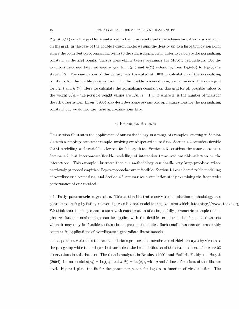
4.1. Fully parametric regression. This section illustrates our variable selection methodology in a
parametric setting by fitting an overdispersed Poisson model to the pox lesions chick data (http://www.statsci.org/-data/general/p
We think that it is important to start with consideration of a simple fully parametric example to em-
phasize that our methodology can be applied with the flexible terms excluded for small data sets
where it may only be feasible to fit a simple parametric model. Such small data sets are reasonably
common in applications of overdispersed generalized linear models.
The dependent variable is the counts of lesions produced on membranes of chick embryos by viruses of
the pox group while the independent variable is the level of dilution of the viral medium. There are 58
observations in this data set. The data is analysed in Breslow (1990) and Podlich, Faddy and Smyth
(2004). In our model g(µi) = log(µi) and h(θi) = log(θi), with g and h linear functions of the dilution
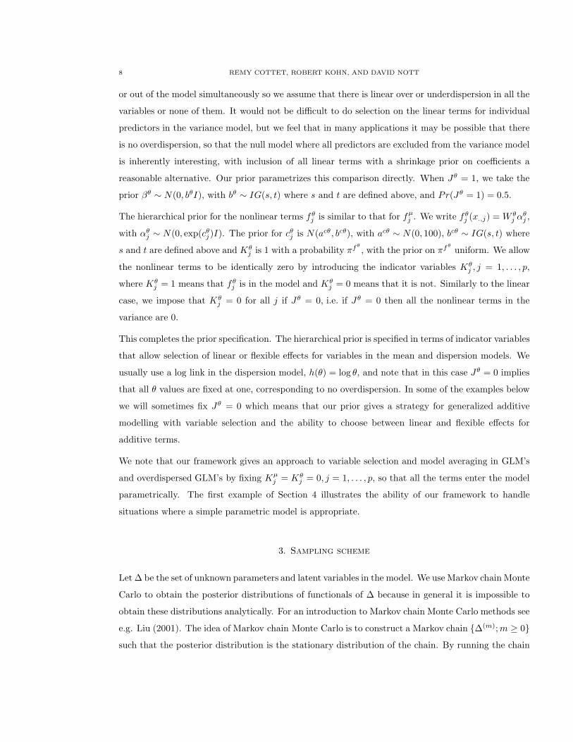
level. Figure 1 plots the fit for the parameter µ and for log θ as a function of viral dilution. The

OVERDISPERSED MODELS 11
posterior probability of overdispersion (that is, the posterior probability of Jθ = 1) is approximately
one strongly suggesting that there is overdispersion, and this is consistent with previous analyses
by Breslow (1990) and Podlich, Faddy and Smyth (2004). The results show that overdispersion is
increasing with an increase of the viral dilution while the lesions count decreases with dilution.
5 10 15 20 25 30
50
100
150
200
250
Viral dilution
Lesi
ons
coun
t
(a)
5 10 15 20 25 30
−6
−5.5
−5
−4.5
−4
−3.5
−3
−2.5
−2
Viral dilution
(b)
Figure 1. Lesions on chick embryos. Plot of the estimated posterior means of mean
and variance parameters as a function of viral dilution together with pointwise 95%
credible intervals. Panel (a) plots estimated values of the parameter µ along with the
data and panel (b) plots estimated values of log θ.
Figure 2 shows a plot of the log-likelihood versus iteration number in our MCMC sampling scheme
as well as the autocorrelation function of the log-likelihood values based on 2000 iterations with 2000
burn in. These plots show that our sampling scheme converges rapidly and mixes well. Corresponding
plots for our other examples (not shown) confirm the excellent properties of our sampling scheme.
The 4000 iterations of our sampler took 280 seconds on a machine with 2.8 GHz processor. For all
the examples considered in this paper programs implementing our sampler were written in Fortran
90.
4.2. Binary logistic regression. This section considers the Pima Indian diabetes dataset obtained
from the UCI repository of machine learning databases (http://www.ics.uci.ecu/MLRepository.html).
The data is analysed by Wahba, Gu, Wang and Chapell (1995). A population of women who were at
least 21 years old, of Pima Indian heritage and living near Phoenix, Arizona, was tested for diabetes
according to World Health Organization criteria. The data were collected by the US National Institute
of Diabetes and Digestive and Kidney Diseases. 724 complete records are used after dropping the

12 REMY COTTET, ROBERT KOHN, AND DAVID NOTT
200 400 600 800 1000 1200 1400 1600 1800 2000254
256
258
260
262
264
Logl
ikel
ihoo
d
Iteration Number
−0.2
0
0.2
0.4
0.6
0.8
Aut
ocor
rela
tion
Figure 2. Lesions on chick embryos. Plot of the log-likelihood versus iteration and
estimated autocorrelation based on 2000 iterations with 2000 burn in.
aberrant cases (as in Yau et al. 2003). The dependent variable is diabetic or not according to WHO
criteria, where a positive test is coded as “1”. There are eight covariates: number of pregnancies,
plasma glucose concentration in an oral glucose tolerance test, diastolic blood pressure (mm Hg),
skin triceps skin fold thickness (mm), 2-Hour serum insulin (mu U/ml), body mass index (weight in
kg/(height in m)2), diabetes pedigree function, and age in years.
This section fits a main effects binary logistic regression to the data. In the framework of section 2, we
are fixing all θi at 1 and so are fitting a generalized linear additive model with g(µi) = log(µi/(1−µi))
that allows for variable selection and choice between flexible and linear effects for the additive terms.
The results are shown in figure 3, with the barplot showing the posterior probabilities of effects for
each predictor being null, linear and flexible. The barplot suggests that the number of pregnancies,
diastolic blood pressure, skin triceps skin fold thickness and 2-Hour serum insulin do not seem to help
predict the occurrence of diabetes when the other covariates are in the model. Figure 3 also shows
that plasma glucose concentration has a strong positive linear effect, and body mass index, diabetes
pedigree function and age have nonlinear effects.

OVERDISPERSED MODELS 13
Our method extends the approach of Yau et al. (2003) to any GAM whereas Yau et al. (2003) rely
on the probit link to turn a binary regression into a regression with Gaussian errors. Our approach
has several other advantages over Yau et al. (2003) as explained in the introduction and section 4.3.
Figure 4 shows the results of applying a variant of the data-based priors approach of Yau et al. (2003)
to the diabetes data.
Since Yau et al. (2003) did not consider logistic regression we need to explain how the data-based
priors approach was applied here. First, the full model was fitted (all flexible terms included) with a
noninformative but proper prior on the cµj parameters (IG(s, t) with s = 27 and t = 1300). Linear
terms are selected together with flexible terms in the approach of Yau et al. (2003). The posterior
medians and variances for the cµj (with the variances inflated by a factor of n) in this fit of the full
model were then used to set means and variances for a normal prior on the cµj in our variable selection
prior similar to Yau et al. (2003). The results of Figure 4 are similar to those shown in Figure 3
but as we have already discussed the data based priors approach is not feasible in general for doing
selection with a large number of terms. Note that in the barplot we only show posterior probabilities
for covariate effects being in or out of the model, since linear and flexible terms are selected together
in the approach of Yau et al. (2003).
We have also compared our approach to that implemented in the GAMLSS R package of Rigby
and Stasinopoulos (2005). We implemented a backward stepwise model selection procedure to select
between null, linear and flexible effects for the predictors starting with the model containing all flexible
terms. We use their generalized AIC criterion with their penalty parameter # set to 2 to compare
models in the backward stepwise procedure. The final model has flexible terms for Age, Glucose
concentration and Body mass index, and a linear term for diabetes function. The fit is shown in
Figure 5.
We also report for this example the acceptance rates for our Metropolis-Hastings proposal at step 4 of
our sampling scheme in the case where there is currently a flexible term in the model for a predictor
and a flexible term is also included in the proposed model. We report acceptance rates for each
predictor where there is posterior probability greater than 0.1 of inclusion of a flexible term. The
corresponding acceptance rates are 19%, 11% and 38% for the three effects selected. These acceptance
rates help to quantify the usefulness of Approximation 2 decribed in the appendix for constructing
the Metropolis-Hastings proposal. Results for this example were based on 4000 iterations of our
sampling scheme with 4000 burn in. The 4000 iterations took 1300 seconds on a machine with 2.8
GHz processor.

14 REMY COTTET, ROBERT KOHN, AND DAVID NOTT
4.3. High dimensional binary logistic regression. This section extends the model for the Pima
Indian dataset to allow for flexible second order interactions. This means that the model potentially
has 36 flexible terms, 8 main effects and 28 interactions. The purpose of this section is to show how
our class of models can handle interactions and that the hierarchical priors allow variable selection
with a large number of terms. This is infeasible with the data-based prior approach of Yau et al.
(2003), as explained in section 1.
We write the generalization of the mean model (2.4) as
g(µi) = β0 +
p∑
j=1
xijβj +
p∑
j=1
fMj (xij) +
p∑
j=1
∑
k<j
f Ijk(xij , xik) .
We have dropped the superscript µ from the βj and the fj because we are dealing with the mean
equation only. However, we write the flexible main effects and interactions as fMj and f I
jk, where M
means main effect and I means an interaction. The prior for the fMj is the same as for the flexible
main effects in Section 2. For the interaction effects we assume that any collection of f Ijk(xi, zi), i =
1, . . . ,m is Gaussian with zero mean and
cov(fjk(x, z), fjk(x′, z′)) = exp(cIjk)Ω(x, x′)Ω(z, z′) ,
where Ω(z, z′) is defined by equation (2.6). This gives a covariance kernel for the fjk that is the
tensor product of univariate covariance kernels (Gu 2002, section 2.4). Once the covariance matrix
for (f Ijk(xij , xik), i = 1, . . . , n) is constructed, we factor it to get a parsimonious representation as in
Section 2. The smoothing parameters cIjk have a similar prior to the cµj in Section 2. To allow for
variable selection of the flexible main effects, let KMj be indicator variables such that KM
j = 0 if fMj
is null and KMj = 1 otherwise. The prior for KM
j is the same as for the Kµj in Section 2. To allow
variable selection on the flexible interaction terms, let KIjk be an indicator variable which is 0 if f I
jk
is null, and is 1 otherwise. To make the bivariate interactions interpretable, we only allow a flexible
interaction between the jth and kth variables if both the flexible main effects are in, i.e., if KMj = 0
or KMk = 0 or both, then KI
jk = 0. If both KMj and KM
k are 1, then
p(KIjk = 1|KM
j ,KMk , πI) = πI
where πI is uniformly distributed. The generation of the interaction effects parameters (αIjk, c
Ijk,K
Ijk)
is similar to the generation of the other parameters in the model. First the indicator variable is
generated from the prior p(KIjk|K
Mj KM
k ). If KIjk = 1 then αI
jk, cIjk are generated as described in the
appendix for the generation of the other parameters, otherwise αIjk is set to zero.

OVERDISPERSED MODELS 15
No interactions were detected when the interaction model were fitted to the data. To test the effective-
ness of the methodology at detecting interactions we also generated observations from the estimated
main effects model, but added an interaction between Diabetes pedigree function and Age. Writing
x and z respectively for these two predictors the interaction term added to our fitted additive model
for logµi/(1 − µi) in the simulation takes the simple multiplicative form xz. Table 4.3 reports the
results of the estimation when the interaction model was fitted to the artificial data, and shows that
the interaction effect between variables 7 and 8 is detected.
Covariate
1 2 3 4 5 6 7 8
Null 0.88 0.00 0.86 0.81 0.76 0.03 0.00 0.00
Linear 0.08 0.58 0.08 0.05 0.11 0.53 0.00 0.00
1 0.00 0.00 0.00 0.00 0.00 0.01 0.03 0.02
2 0.42 0.01 0.03 0.05 0.13 0.24 0.21
3 0.06 0.02 0.02 0.00 0.02 0.03
4 0.14 0.04 0.03 0.07 0.07
5 0.13 0.03 0.06 0.06
6 0.44 0.023 0.23
7 1.00 1.00
8 1.00
Table 1. Simulated diabetes data with interaction. Posterior probabilities of null,
linear and flexible main effects and flexible interaction effects. The table is interpreted
as follows for covariate 4. The posterior probabilities of a null, linear and flexible
main effect are 0.81, 0.05 and 0.14. The posterior probability of a flexible interaction
between covariates 3 and 4 is 0.02. Other entries in the table are interpreted similarly.
4.4. Double Binomial model. This example considers a dataset in Moore and Tsiatis (1991) and
analyzed by Aerts and Claeskens (1997) using a local beta binomial model. An iron supplement was
given to 58 female rats at various dose levels. The rats were then made pregnant and sacrificed after
3 weeks. The litter size and the number of fetuses dead were recorded as well as the hemoglobin levels
of the mothers. We fitted a double binomial model to the data to try to explain the proportion of
dead foetuses with the level of hemoglobin of the mother and litter size as covariates.
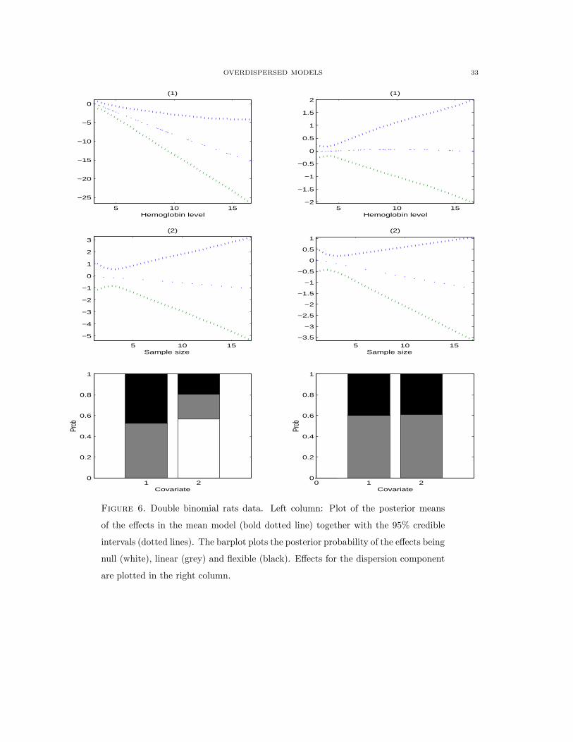
16 REMY COTTET, ROBERT KOHN, AND DAVID NOTT
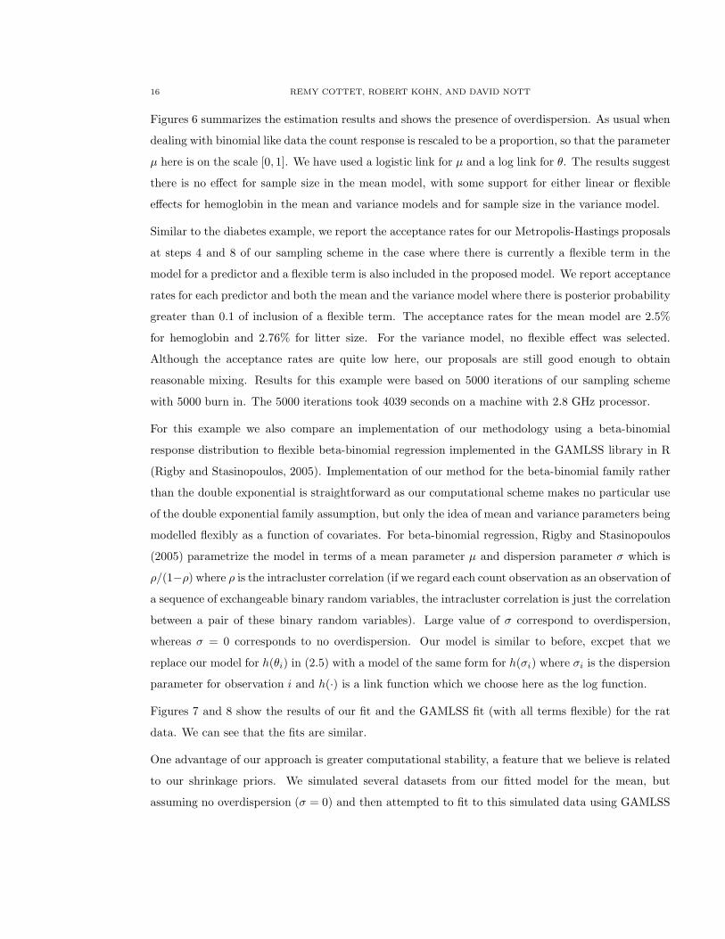
Figures 6 summarizes the estimation results and shows the presence of overdispersion. As usual when
dealing with binomial like data the count response is rescaled to be a proportion, so that the parameter
µ here is on the scale [0, 1]. We have used a logistic link for µ and a log link for θ. The results suggest
there is no effect for sample size in the mean model, with some support for either linear or flexible
effects for hemoglobin in the mean and variance models and for sample size in the variance model.
Similar to the diabetes example, we report the acceptance rates for our Metropolis-Hastings proposals
at steps 4 and 8 of our sampling scheme in the case where there is currently a flexible term in the
model for a predictor and a flexible term is also included in the proposed model. We report acceptance
rates for each predictor and both the mean and the variance model where there is posterior probability
greater than 0.1 of inclusion of a flexible term. The acceptance rates for the mean model are 2.5%
for hemoglobin and 2.76% for litter size. For the variance model, no flexible effect was selected.
Although the acceptance rates are quite low here, our proposals are still good enough to obtain
reasonable mixing. Results for this example were based on 5000 iterations of our sampling scheme
with 5000 burn in. The 5000 iterations took 4039 seconds on a machine with 2.8 GHz processor.
For this example we also compare an implementation of our methodology using a beta-binomial
response distribution to flexible beta-binomial regression implemented in the GAMLSS library in R
(Rigby and Stasinopoulos, 2005). Implementation of our method for the beta-binomial family rather
than the double exponential is straightforward as our computational scheme makes no particular use
of the double exponential family assumption, but only the idea of mean and variance parameters being
modelled flexibly as a function of covariates. For beta-binomial regression, Rigby and Stasinopoulos
(2005) parametrize the model in terms of a mean parameter µ and dispersion parameter σ which is
ρ/(1−ρ) where ρ is the intracluster correlation (if we regard each count observation as an observation of
a sequence of exchangeable binary random variables, the intracluster correlation is just the correlation
between a pair of these binary random variables). Large value of σ correspond to overdispersion,
whereas σ = 0 corresponds to no overdispersion. Our model is similar to before, excpet that we
replace our model for h(θi) in (2.5) with a model of the same form for h(σi) where σi is the dispersion
parameter for observation i and h(·) is a link function which we choose here as the log function.
Figures 7 and 8 show the results of our fit and the GAMLSS fit (with all terms flexible) for the rat
data. We can see that the fits are similar.
One advantage of our approach is greater computational stability, a feature that we believe is related
to our shrinkage priors. We simulated several datasets from our fitted model for the mean, but
assuming no overdispersion (σ = 0) and then attempted to fit to this simulated data using GAMLSS
OVERDISPERSED MODELS 17
and our Bayesian approach with a beta-binomial model. The Bayesian approach produces satisfactory
results, but attempting to fit the model in GAMLSS even with only an intercept and no covariates in
the variance model results in convergence problems that are not easily resolved (D.M. Stasinopoulos,
personal communication). However, the GAMLSS fit is faster, and we have found the GAMLSS
package to be very useful for the exploratory examination of many potential models.
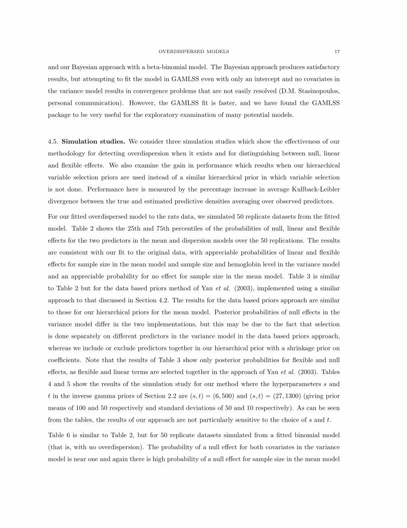
4.5. Simulation studies. We consider three simulation studies which show the effectiveness of our
methodology for detecting overdispersion when it exists and for distinguishing between null, linear
and flexible effects. We also examine the gain in performance which results when our hierarchical
variable selection priors are used instead of a similar hierarchical prior in which variable selection
is not done. Performance here is measured by the percentage increase in average Kullback-Leibler
divergence between the true and estimated predictive densities averaging over observed predictors.
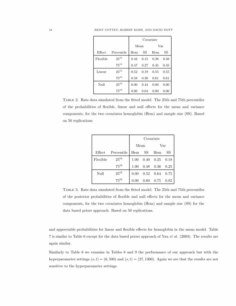
For our fitted overdispersed model to the rats data, we simulated 50 replicate datasets from the fitted
model. Table 2 shows the 25th and 75th percentiles of the probabilities of null, linear and flexible
effects for the two predictors in the mean and dispersion models over the 50 replications. The results
are consistent with our fit to the original data, with appreciable probabilities of linear and flexible
effects for sample size in the mean model and sample size and hemoglobin level in the variance model
and an appreciable probability for no effect for sample size in the mean model. Table 3 is similar
to Table 2 but for the data based priors method of Yau et al. (2003), implemented using a similar
approach to that discussed in Section 4.2. The results for the data based priors approach are similar
to those for our hierarchical priors for the mean model. Posterior probabilities of null effects in the
variance model differ in the two implementations, but this may be due to the fact that selection
is done separately on different predictors in the variance model in the data based priors approach,
whereas we include or exclude predictors together in our hierarchical prior with a shrinkage prior on
coefficients. Note that the results of Table 3 show only posterior probabilities for flexible and null
effects, as flexible and linear terms are selected together in the approach of Yau et al. (2003). Tables
4 and 5 show the results of the simulation study for our method where the hyperparameters s and
t in the inverse gamma priors of Section 2.2 are (s, t) = (6, 500) and (s, t) = (27, 1300) (giving prior
means of 100 and 50 respectively and standard deviations of 50 and 10 respectively). As can be seen
from the tables, the results of our approach are not particularly sensitive to the choice of s and t.
Table 6 is similar to Table 2, but for 50 replicate datasets simulated from a fitted binomial model
(that is, with no overdispersion). The probability of a null effect for both covariates in the variance
model is near one and again there is high probability of a null effect for sample size in the mean model
18 REMY COTTET, ROBERT KOHN, AND DAVID NOTT
Covariate
Mean Var
Effect Percentile Hem SS Hem SS
Flexible 25th
0.42 0.15 0.38 0.38
75th
0.47 0.27 0.45 0.45
Linear 25th
0.52 0.19 0.55 0.55
75th
0.58 0.30 0.61 0.61
Null 25th
0.00 0.44 0.00 0.00
75th
0.00 0.64 0.00 0.00
Table 2. Rats data simulated from the fitted model. The 25th and 75th percentiles
of the probabilities of flexible, linear and null effects for the mean and variance
components, for the two covariates hemoglobin (Hem) and sample size (SS). Based
on 50 replications
Covariate
Mean Var
Effect Percentile Hem SS Hem SS
Flexible 25th 1.00 0.40 0.25 0.18
75th 1.00 0.48 0.36 0.25
Null 25th 0.00 0.52 0.64 0.75
75th 0.00 0.60 0.75 0.82
Table 3. Rats data simulated from the fitted model. The 25th and 75th percentiles
of the posterior probabilities of flexible and null effects for the mean and variance
components, for the two covariates hemoglobin (Hem) and sample size (SS) for the
data based priors approach. Based on 50 replications.
and appreciable probabilities for linear and flexible effects for hemoglobin in the mean model. Table
7 is similar to Table 6 except for the data based priors approach of Yau et al. (2003). The results are
again similar.
Similarly to Table 6 we examine in Tables 8 and 9 the performance of our approach but with the
hyperparameter settings (s, t) = (6, 500) and (s, t) = (27, 1300). Again we see that the results are not
sensitive to the hyperparameter settings.

OVERDISPERSED MODELS 19
Covariate
Mean Var
Effect Percentile Hem SS Hem SS
Flexible 25th 0.10 0.04 0.11 0.10
75th 0.13 0.06 0.13 0.13
Linear 25th 0.86 0.27 0.87 0.88
75th 0.89 0.33 0.89 0.90
Null 25th 0.00 0.60 0.00 0.00
75th 0.01 0.69 0.00 0.00
Table 4. Rats data simulated from the fitted model. The 25th and 75th percentiles
of the probabilities of flexible, linear and null effects for the mean and variance
components, for the two covariates hemoglobin (Hem) and sample size (SS). Based
on 50 replications and hyperparameter settings (s, t) = (27, 1300).
Covariate
Mean Var
Effect Percentile Hem SS Hem SS
Flexible 25th 0.09 0.03 0.11 0.10
75th 0.12 0.05 0.14 0.13
Linear 25th 0.86 0.23 0.86 0.87
75th 0.90 0.28 0.89 0.90
Null 25th 0.00 0.66 0.00 0.00
75th 0.02 0.73 0.00 0.00
Table 5. Rats data simulated from the fitted model. The 25th and 75th percentiles
of the probabilities of flexible, linear and null effects for the mean and variance
components, for the two covariates hemoglobin (Hem) and sample size (SS). Based
on 50 replications and hyperparameter settings (s, t) = (6, 500).
Table 10 shows probabilities of null, linear and flexible effects for the eight covariates in the diabetes
example for 50 simulated replicate datasets from an additive model fitted to the real data. Again the
results are consistent with out fit to the full model, with high probability of a null effect for covariates
1, 3, 4 and 5 (the number of pregnancies, diastolic blood pressure, skin triceps skin fold thickness and

20 REMY COTTET, ROBERT KOHN, AND DAVID NOTT
Covariate
Mean Var
Effect Percentile Hem SS Hem SS
Flexible 25th 0.40 0.08 0.00 0.00
75th 0.43 0.22 0.00 0.00
Linear 25th 0.57 0.12 0.00 0.00
75th 0.60 0.36 0.00 0.00
Null 25th 0.00 0.43 0.99 0.99
75th 0.00 0.79 0.99 0.99
Table 6. Rats simulated data from a fitted binomial model with no overdispersion.
The 25th and 75th percentiles of the probabilities of flexible, linear and null effects
are given for the mean and variance components, for the two covariates hemoglobin
(Hem) and sample size (SS). Based on 50 replications.
Covariate
Mean Var
Effect Percentile Hem SS Hem SS
Flexible 25th 1.00 0.47 0.00 0.00
75th 1.00 0.51 0.00 0.00
Null 25th 0.00 0.49 1.00 1.00
75th 0.00 0.53 1.00 1.00
Table 7. Rats simulated data from a fitted binomial model with no overdispersion.
The 25th and 75th percentiles of the posterior probabilities of flexible and null effects
are given for the mean and variance components, for the two covariates hemoglobin
(Hem) and sample size (SS), and the data based priors approach. Based on 50
replications.
2-Hour serum insulin respectively), an appreciable probability of a linear effect for covariate 2 (plasma
glucose concentration) and high probabilities of nonlinear effects for covariates 6, 7 and 8 (body mass
index, diabetes pedigree function and age). Table 11 is similar to 10 but for the data based priors
approach of Yau et al. (2003). Again the results are similar to those obtained using our hierarchical
priors.

OVERDISPERSED MODELS 21
Covariate
Mean Var
Effect Percentile Hem SS Hem SS
Flexible 25th 0.10 0.02 0.00 0.00
75th 0.14 0.05 0.02 0.01
Linear 25th 0.86 0.10 0.00 0.00
75th 0.90 0.19 0.12 0.13
Null 25th 0.00 0.75 0.86 0.86
75th 0.00 0.87 1.00 1.00
Table 8. Rats simulated data from a fitted binomial model with no overdispersion.
The 25th and 75th percentiles of the probabilities of flexible, linear and null effects
are given for the mean and variance components, for the two covariates hemoglobin
(Hem) and sample size (SS). Based on 50 replications and hyperparameter settings
(s, t) = (6, 500).
Covariate
Mean Var
Effect Percentile Hem SS Hem SS
Flexible 25th 0.10 0.02 0.00 0.00
75th 0.14 0.05 0.03 0.03
Linear 25th 0.86 0.14 0.01 0.01
75th 0.90 0.25 0.23 0.24
Null 25th 0.00 0.67 0.73 0.73
75th 0.00 0.83 0.99 0.99
Table 9. Rats simulated data from a fitted binomial model with no overdispersion.
The 25th and 75th percentiles of the probabilities of flexible, linear and null effects
are given for the mean and variance components, for the two covariates hemoglobin
(Hem) and sample size (SS). Based on 50 replications and hyperparameter settings
(s, t) = (27, 1300).
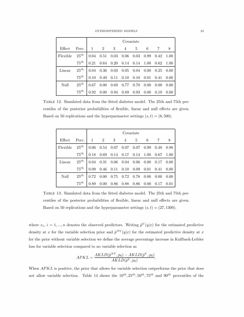
Similar to Table 10 we examine in Tables 12 and 13 the performance of our approach but with the
hyperparameter settings (s, t) = (6, 500) and (s, t) = (27, 1300). Again we see that the results are not
particularly sensitive to the hyperparameter settings.

22 REMY COTTET, ROBERT KOHN, AND DAVID NOTT
Covariate
Effect Perc. 1 2 3 4 5 6 7 8
Flexible 25th 0.03 0.55 0.06 0.05 0.04 0.62 0.35 0.99
75th 0.06 0.61 0.11 0.11 0.12 0.97 0.54 1.00
Linear 25th 0.03 0.39 0.04 0.03 0.04 0.03 0.19 0.00
75th 0.05 0.45 0.08 0.09 0.08 0.38 0.40 0.01
Null 25th 0.88 0.00 0.80 0.79 0.82 0.00 0.04 0.00
75th 0.94 0.00 0.90 0.91 0.92 0.00 0.46 0.00
Table 10. Simulated data from the fitted diabetes model. The 25th and 75th per-
centiles of the posterior probabilities of flexible, linear and null effects are given.
Based on 50 replications.
Covariate
Effect Perc. 1 2 3 4 5 6 7 8
Flexible 25th 0.36 1.00 0.35 0.34 0.28 1.00 0.26 1.00
75th 0.52 1.00 0.49 0.49 0.48 1.00 1.00 1.00
Null 25th 0.48 0.00 0.51 0.51 0.52 0.00 0.00 0.00
75th 0.64 0.00 0.65 0.66 0.72 0.00 0.74 0.00
Table 11. Simulated data from the fitted diabetes model. The 25th and 75th per-
centiles of the posterior probabilities of flexible and null effects are given for the data
based priors approach. Based on 50 replications.
We now compare the performance of our hierarchical variable selection priors with the same prior but
where all terms are flexible (that is, no variable selection is carried out). Our measure of performance
is the Kullback-Leibler divergence, averaged over the observed covariates.
In estimating the true response distribution p0(y|x) using an estimate p(y|x) where x denotes the
covariates, the Kullback-Leibler divergence is defined as
KL(p(·|x), p0(·|x)) =
∫
p0(y|x) log
[
p(y|x)
p0(y|x)
]
dy.
We define the average Kullback-Leibler divergence as
AKLD(p, p0) =1
n
n∑
i=1
KL(p(·|xi), p0(·|xi))
OVERDISPERSED MODELS 23
Covariate
Effect Perc. 1 2 3 4 5 6 7 8
Flexible 25th 0.04 0.51 0.03 0.06 0.03 0.99 0.42 1.00
75th 0.21 0.64 0.20 0.14 0.14 1.00 0.62 1.00
Linear 25th 0.04 0.36 0.03 0.05 0.04 0.00 0.25 0.00
75th 0.10 0.49 0.11 0.10 0.10 0.01 0.41 0.00
Null 25th 0.67 0.00 0.69 0.77 0.78 0.00 0.00 0.00
75th 0.92 0.00 0.94 0.89 0.93 0.00 0.19 0.00
Table 12. Simulated data from the fitted diabetes model. The 25th and 75th per-
centiles of the posterior probabilities of flexible, linear and null effects are given.
Based on 50 replications and the hyperparmaeter settings (s, t) = (6, 500).
Covariate
Effect Perc. 1 2 3 4 5 6 7 8
Flexible 25th 0.06 0.54 0.07 0.07 0.07 0.99 0.48 0.98
75th 0.18 0.69 0.14 0.17 0.14 1.00 0.67 1.00
Linear 25th 0.04 0.31 0.06 0.04 0.06 0.00 0.17 0.00
75th 0.09 0.46 0.11 0.10 0.09 0.01 0.41 0.00
Null 25th 0.72 0.00 0.75 0.72 0.78 0.00 0.00 0.00
75th 0.89 0.00 0.86 0.88 0.86 0.00 0.17 0.01
Table 13. Simulated data from the fitted diabetes model. The 25th and 75th per-
centiles of the posterior probabilities of flexible, linear and null effects are given.
Based on 50 replications and the hyperparameter settings (s, t) = (27, 1300).
where xi, i = 1, ..., n denotes the observed predictors. Writing pV (y|x) for the estimated predictive
density at x for the variable selection prior and pNV (y|x) for the estimated predictive density at x
for the prior without variable selection we define the average percentage increase in Kullback-Leibler
loss for variable selection compared to no variable selection as
APKL =AKLD(pNV , p0) −AKLD(pV , p0)
AKLD(pV , p0).
When APKL is positive, the prior that allows for variable selection outperforms the prior that does
not allow variable selection. Table 14 shows the 10th, 25th, 50th, 75th and 90th precentiles of the

24 REMY COTTET, ROBERT KOHN, AND DAVID NOTT
APKL for the 50 replicate data sets generated in our simulation study for the diabetes data, the
rats data when no overdispersion is present and the rats data when overdispersion is present. The
table shows that the median percentage increase in APKL is positive for all three cases, indicating
an improvement for using our hierarchical variable selection prior compared to not doing variable
selection. Furthermore, for the rats data with no overdispersion, even the 10th percentile exceeds
28%.
Dataset Percentiles
10th 25th 50th 75th 90th
Diabetes -14.49 -1.17 16.74 40.85 64.14
Rats with overdispersion -13.92 -5.18 9.08 30.48 62.20
Rats with no overdispersion 28.67 67.55 155.52 293.43 734.54
Table 14. 10th, 25th, 50th, 75th and 90th precentiles in the percentage increase in
Kullback-leibler divergence when no variable selection is carried out compared to
when variable selection is carried out. The results are based on 50 replications for
the diabetes data, rats data when no overdispersion is present and rats data when
overdispersion is present.
5. Conclusion
The article develops a general Bayesian framework for variable selection and model averaging in
generalized linear models that allows for over or under dispersion. The priors and sampling are
innovative and the flexibility of the approach is demonstrated using a number of examples, ranging
from fully parametric to fully nonparametric.
There are a number of natural extensions to the work described here. Although we have implemented
our approach to flexible regression for the mean and variance using the double exponential family
of distributions, it is easy to implement a similar approach using other distributional families for
overdispersed count data such as the beta-binomial and negative binomial. We have demonstrated
use of the beta-binomial in one of our real data examples. Flexible modelling of multivariate data
could also be easily accommodated in our framework by incorporation of other kinds of random effects
apart from those involved in our nonparametric functional forms. These and other extensions are the
subject of ongoing research.

OVERDISPERSED MODELS 25
Acknowledgements
This work was supported by an Australian Research Council Grant. We thank Dr Mikis Stasinopoulos
for a quick and helpful response to some questions about the GAMLSS package.
6. Appendix
This section gives details of the sampling scheme in Section 3. Most of the steps involve an application
of the Metropolis-Hastings method based on one of the following two approximations to the conditional
densities.
Approximation 1
Here we seek to generate a parameter ψ from its full conditional p(ψ|y,∆\ψ), where ∆ consists of all
the parameters and latent variables used in the sampling scheme and ∆\ψ means all of ∆ excluding
ψ. We write
p(ψ|y,∆\ψ) ∝ p(y|ψ,∆\ψ)p(ψ|∆\ψ)(6.1)
∝ exp(−l(ψ))
where l(ψ) is the negative of the logarithm of the left side of (6.1) and for convenience the dependence
of l(·) on ∆\ψ is omitted.
Let ψ be the minimum of l(ψ) and Ψ = ∂2l(ψ)/∂ψ∂ψ. We approximate the full conditional of ψ
by a normal density with mean ψ and covariance matrix Ψ−1. Generally we find ψ using numerical
optimization routines from the NAG or IMSL libraries and have not experienced any difficulties of
convergence. As a practical matter, there may be a substantial benefit to early stopping of the
optimization in constructing our proposals after just a few or even one step. Just a few steps gives a
good approximation to ψ and this suffices to obtain good proposals with the early stopping resulting
in a considerable saving in computation time since several applications of Approximation 1 are done
at every iteration of the sampling scheme.
Approximation 2
Here we seek to generate parameters ψ and w as a block from their joint conditional density. We
assume that p(y|ψ,w,∆\ ψ,w) = p(y|ψ,∆\ ψ,w) and p(ψ|w,∆\ ψ,w) = p(ψ|w) is Gaussian.
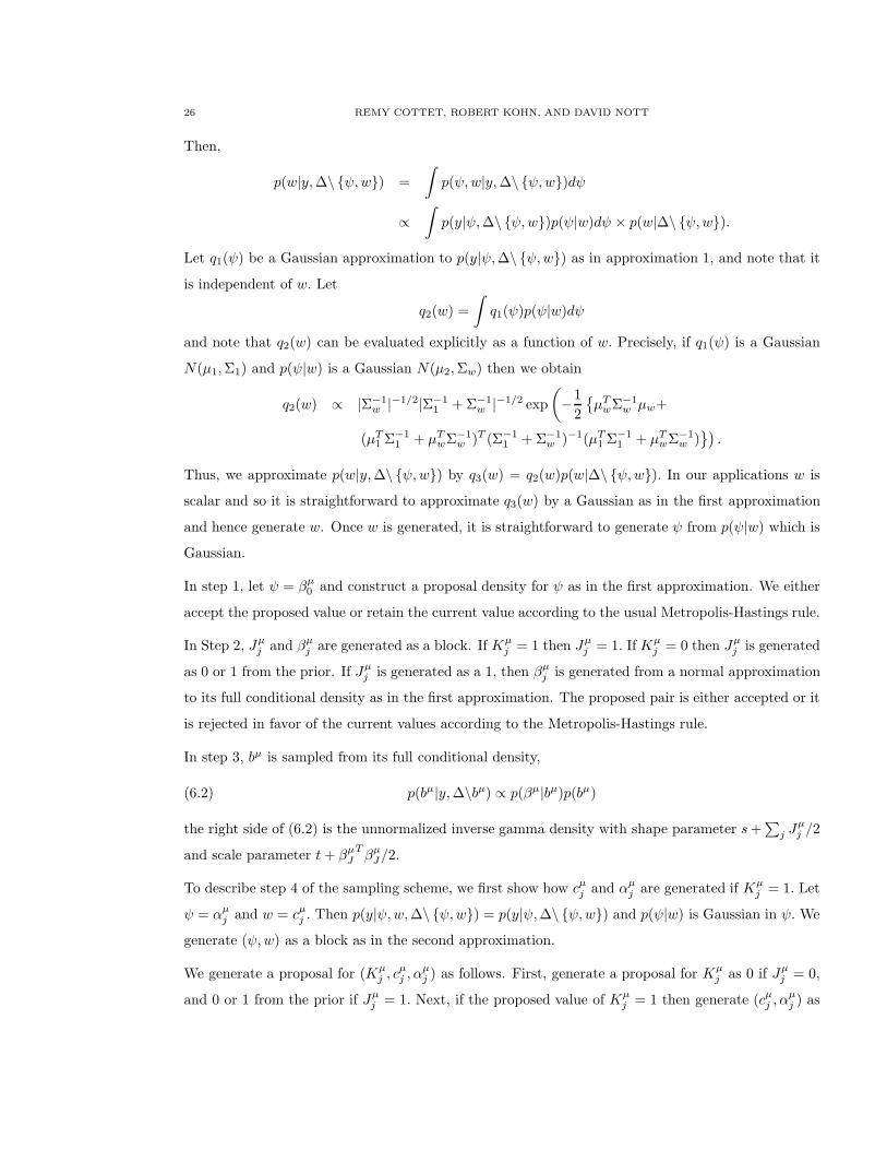
26 REMY COTTET, ROBERT KOHN, AND DAVID NOTT
Then,
p(w|y,∆\ ψ,w) =
∫
p(ψ,w|y,∆\ ψ,w)dψ
∝
∫
p(y|ψ,∆\ ψ,w)p(ψ|w)dψ × p(w|∆\ ψ,w).
Let q1(ψ) be a Gaussian approximation to p(y|ψ,∆\ ψ,w) as in approximation 1, and note that it
is independent of w. Let
q2(w) =
∫
q1(ψ)p(ψ|w)dψ
and note that q2(w) can be evaluated explicitly as a function of w. Precisely, if q1(ψ) is a Gaussian
N(µ1,Σ1) and p(ψ|w) is a Gaussian N(µ2,Σw) then we obtain
q2(w) ∝ |Σ−1w |−1/2|Σ−1
1 + Σ−1w |−1/2 exp
(
−1
2
µTwΣ−1
w µw+
(µT1 Σ−1
1 + µTwΣ−1
w )T (Σ−11 + Σ−1
w )−1(µT1 Σ−1
1 + µTwΣ−1
w ))
.
Thus, we approximate p(w|y,∆\ ψ,w) by q3(w) = q2(w)p(w|∆\ ψ,w). In our applications w is
scalar and so it is straightforward to approximate q3(w) by a Gaussian as in the first approximation
and hence generate w. Once w is generated, it is straightforward to generate ψ from p(ψ|w) which is
Gaussian.
In step 1, let ψ = βµ0 and construct a proposal density for ψ as in the first approximation. We either
accept the proposed value or retain the current value according to the usual Metropolis-Hastings rule.
In Step 2, Jµj and βµ
j are generated as a block. If Kµj = 1 then Jµ
j = 1. If Kµj = 0 then Jµ
j is generated
as 0 or 1 from the prior. If Jµj is generated as a 1, then βµ
j is generated from a normal approximation
to its full conditional density as in the first approximation. The proposed pair is either accepted or it
is rejected in favor of the current values according to the Metropolis-Hastings rule.
In step 3, bµ is sampled from its full conditional density,
(6.2) p(bµ|y,∆\bµ) ∝ p(βµ|bµ)p(bµ)
the right side of (6.2) is the unnormalized inverse gamma density with shape parameter s+∑
j Jµj /2
and scale parameter t+ βµJ
Tβµ
J/2.
To describe step 4 of the sampling scheme, we first show how cµj and αµj are generated if Kµ
j = 1. Let
ψ = αµj and w = cµj . Then p(y|ψ,w,∆\ ψ,w) = p(y|ψ,∆\ ψ,w) and p(ψ|w) is Gaussian in ψ. We
generate (ψ,w) as a block as in the second approximation.
We generate a proposal for (Kµj , c
µj , α
µj ) as follows. First, generate a proposal for Kµ
j as 0 if Jµj = 0,
and 0 or 1 from the prior if Jµj = 1. Next, if the proposed value of Kµ
j = 1 then generate (cµj , αµj ) as

OVERDISPERSED MODELS 27
outlined above. Then, we accept or reject the block proposal according to the Metropolis-Hastings
rule.
In step 5, acµ and bcµ can be updated from their full conditional distributions. We have
p(acµ|∆\acµ) ∝ p(acµ)p(cµ|acµ, bcµ)
and we recognize the right hand side as an unnormalized normal density. We have
p(acµ|∆\acµ) = N
(
∑
j Kµj
bcµ+
1
100
)
−1(cµ)T cµ
bcµ,
(
∑
j Kµj
bcµ+
1
100
)
−1
.
Also,
p(bcµ|∆\bcµ) ∝ p(bcµ)p(cµ|acµ, bcµ)
and we recognize the right hand side as an unnormalized inverse gamma density. We have
p(bcµ|∆\bcµ) = IG
(
s+
∑
j Kµj
2, t+
1
2(cµ − acµ)T (cµ − acµ)
)
.
Step 6 is similar to step 1, except that a multivariate normal approximation is used to generate βθ
given Jθ = 1 and the current values of other parameters. Step 7 is similar to step 3 and
p(bθ|∆\bθ, Jθ, Jθ = 1) = IG
(
s+q + 1
2, t+
1
2
(
βθ)Tβθ
)
.
Steps 8 and 9 are performed similarly to steps 4 and 5.
References
Aerts, M. and Claskens, G. (1997), “Local polynomial estimation in multiparameter models,” Journal
of the American Statistical Association, 92, 1536–1545.
Breslow, N. (1990), “Further studies in the variability of pock counts,” Statistics in Medicine, 9,
615–626.
Breslow, N. and Clayton, D. (1993), “Approximate inference in generalized linear mixed models,”
Journal of the American Statistical Association, 88, 9–25.
Brezger, A. and Lang, S. (2005), “Generalized additive structured regression based on Bayesian P-
splines,” Computational Statistics and Data Analysis, 50, 967–991.
Davidian, M. and Carroll, R. (1987), “Variance function estimation,” Journal of the American Sta-
tistical Association, 82, 1079–1091.
— (1988), “A note on extended quasilikelihood,” Journal of the Royal Statistical Society B, 50, 74–82.
Davidian, M. and Giltinan, D. (1995), Nonlinear Models for Repeated Measurement Data, New York:
Chapman and Hall.

28 REMY COTTET, ROBERT KOHN, AND DAVID NOTT
Efron, B. (1986), “Double exponential families and their use in generalised linear regression,” Journal
of the American Statistical Association, 81, 709–721.
Eilers, P. H. C. and Marx, B. D. (1996), “Flexible Smoothing with B-splines and Penalties with
Rejoinder,” Statistical Science, 11, 89–121.
Faddy, M. (1997), “Extended Poisson process modelling and analysis of count data,” Biometrical
Journal, 39, 431–440.
Gelfand, A. and Dalal, S. (1990), “A note on overdispersed exponential families,” Biometrika, 77,
55–64.
Gelfand, A., Dey, D., and Peng, F. (1997), “Overdispersed generalized linear models,” Journal of
Statistical Planning and Inference, 64, 93–107.
Gu, C. (2002), Smoothing spline ANOVA models, New York: Springer-Verlag.
Hastie, T. (1996), “Pseudosplines,” Journal of the Royal Statistical Society B, 58, 379–396.
Hastie, T. and Tibshirani, R. (1990), Generalized Additive Models, New York: Chapman and Hall.
Jorgensen, B. (1997), The Theory of Dispersion Models, London: Chapman and Hall.
Lee, Y. and Nelder, J. (1996), “Hierarchical generalized linear models (with Discussion),” Journal of
the Royal Statistical Society B, 58, 619–678.
Lin, X. and Zhang, D. (1999), “Inference in generalized additive mixed models by using smoothing
splines,” Journal of the Royal Statistical Society B, 61, 381–400.
Liu, J. (2001), Monte Carlo Strategies in Scientific Computing, New York: Springer-Verlag.
McCullagh, P. and Nelder, J. (1989), Generalized Linear Models, London: Chapman and Hall, 2nd
ed.
Moore, D. and Tsiatis, A. (1991), “Robust estimation of the variance in moment methods for extra-
binomial and extra-Poisson variation,” Biometrics, 47, 383–401.
Nelder, J. and Pregibon, D. (1987), “An extended quasi-likelihood function,” Biometrika, 74, 221–232.
Nelder, J. and Wedderburn, R. (1972), “Generalized linear models,” Journal of the Royal Statistical
Society B, 135, 370–384.
Nott, D. (2004), “Semiparametric estimation of mean and variance functions for non-Gaussian data,”
Working paper.
Peck, C., Beal, S., Sheiner, L., and Nichols, A. (1984), “Extended least squares nonlinear regression:
A possible solution to the choice of weights problem in analysis of individual pharmacokinetic data,”
Journal of Pharmacokinetics and Biopharmaceutics, 12, 545–558.
Podlich, H., Faddy, M., and Smyth, G. (2004), “Semi-parametric extended Poisson process models,”
Statistics and Computing, 14, 311–321.
OVERDISPERSED MODELS 29
Rigby, R. and Stasinopoulos, D. (2005), “Generalized additive models for location, scale and shape,”
Applied Statistics, 54, 1–38.
Ruppert, D., Wand, M., and Carroll, R. (2003), Semiparametric regression, Cambridge: Cambridge
University Press.
Shively, S., Kohn, R., and Wood, S. (1999), “Variable selection and function estimation in additive
nonparametric regression using a data based prior (with discussion),” Journal of the American
Statistical Association, 94, 777–807.
Smith, M. and Kohn, R. (1996), “Nonparametric Regression Using Bayesian Variable Selection,”
Journal of Econometrics, 75, 317–344.
Smyth, G. (1989), “Generalized linear models with varying dispersion,” Journal of the Royal Statistical
Society B, 51, 47–60.
Smyth, G. K. and Verbyla, A. P. (1999), “Adjusted likelihood methods for modelling dispersion in
generalized linear models,” Environmetrics, 10, 696–709.
Wahba, G., Wang, Y., Gu, C., Klein, R., and Klein, B. (1995), “Smoothing spline ANOVA for expo-
nential families, with application to the Wisconsin Epidemiological Study of Diabetic Retinopathy,”
Annals of Statistics, 23, 1865–1895.
Wedderburn, R. (1974), “Quasi-likelihoods functions, generalized linear models and the Gauss-Newton
method,” Biometrika, 61, 439–447.
Wild, C. and Yee, T. (1996), “Additive extensions to generalized estimating equation methods,”
Journal of the Royal Statistical Society B, 58, 711–725.
Yau, P., Kohn, R., and Wood, S. (2003), “Bayesian variable selection and model averaging in high-
dimensional multinomial nonparametric regression,” Journal of Computational and Graphical Sta-
tistics, 12, 23–54.
Yee, T. and Wild, C. (1996), “Vector Generalized Additive Models,” Journal of the Royal Statistical
Society B, 58, 481–493.
University of New South Wales, Sydney, Australia

30 REMY COTTET, ROBERT KOHN, AND DAVID NOTT
0 5 10 15
−0.5
0
0.5
1
# times pregnant
(1)
50 100 150
0
2
4
6
Glucose concentration
(2)
40 60 80 100 120
−1.5
−1
−0.5
0
0.5
1
Diastolic blood pressure
(3)
0 20 40 60 80
−0.6
−0.4
−0.2
0
0.2
0.4
Triceps skin thickness
(4)
0 200 400 600 800
−1
−0.5
0
0.5
2−Hour serum insulin
(5)
20 40 60
0
5
10
Body mass index
(6)
0.5 1 1.5 2
−1
0
1
2
3
4
Diabetes function
(7)
40 60 80
−4
−2
0
2
Age
(8)
1 2 3 4 5 6 7 80
0.2
0.4
0.6
0.8
1
Pro
b
Covariate
Figure 3. Logistic Diabetes data. Plots of the posterior means of the covariate
effects at the design points (dotted bold line) and 95% credible intervals (dotted
lines). The barplot gives the posterior probability of each covariate function being
null (white), linear (grey) and flexible (black).

OVERDISPERSED MODELS 31
0 5 10 15−1
−0.5
0
0.5
1
# times pregnant
Xβ
i in
me
an
1
50 100 1500
2
4
6
8
Glucose concentration X
βi in
me
an
2
40 60 80 100 120−1
−0.5
0
0.5
1
Diastolic blood pressure
Xβ
i in
me
an
3
0 20 40 60 80−1
−0.5
0
0.5
1
Triceps skin thickness
Xβ
i in
me
an
4
0 200 400 600 800−1
−0.5
0
0.5
1
2−Hour serum insulin
Xβ
i in
me
an
5
20 30 40 50 600
2
4
6
8
Body mass index X
βi in
me
an
6
0.5 1 1.5 2
−2
−1
0
1
Diabetes function
Xβ
i in
me
an
7
30 40 50 60 70 80−6
−4
−2
0
2
Age
Xβ
i in
me
an
8
1 2 3 4 5 6 7 80
0.5
1
Pro
b
Covariate
9
Figure 4. Logistic Diabetes data. Plots of the posterior means of the covariate
effects at the design points (dotted bold line) and 95% credible intervals (dotted
lines) for data based priors approach. The barplot gives the posterior probability of
each covariate function being in or out of the model.

32 REMY COTTET, ROBERT KOHN, AND DAVID NOTT
50 100 150 200
−6−4
−20
2
Glucose oncentration
Xbet
a_i in
mea
n
20 30 40 50 60
−3−2
−10
12
3
Body mass index
Xbet
a_i in
mea
n
0.0 0.5 1.0 1.5 2.0 2.5
0.0
0.5
1.0
1.5
Diabetes function
Xbet
a_i in
mea
n
20 30 40 50 60 70 80
−4−3
−2−1
01
2
Age
Xbet
a_i in
mea
n
Figure 5. Logistic Diabetes data. Plots of the estimated covariate effects (solid line)
and 95% credible intervals (dotted lines) using GAMLSS and a backward stepwise
model selection procedure with generalized AIC criterion for model selection.
OVERDISPERSED MODELS 33
5 10 15
−25
−20
−15
−10
−5
0
Hemoglobin level
(1)
5 10 15
−5
−4
−3
−2
−1
0
1
2
3
Sample size
(2)
1 20
0.2
0.4
0.6
0.8
1
Prob
Covariate
5 10 15−2
−1.5
−1
−0.5
0
0.5
1
1.5
2(1)
Hemoglobin level
5 10 15−3.5
−3
−2.5
−2
−1.5
−1
−0.5
0
0.5
1(2)
Sample size
0 1 20
0.2
0.4
0.6
0.8
1
Prob
Covariate
Figure 6. Double binomial rats data. Left column: Plot of the posterior means
of the effects in the mean model (bold dotted line) together with the 95% credible
intervals (dotted lines). The barplot plots the posterior probability of the effects being
null (white), linear (grey) and flexible (black). Effects for the dispersion component
are plotted in the right column.

34 REMY COTTET, ROBERT KOHN, AND DAVID NOTT
5 10 15
−8
−6
−4
−2
0
Hemoglobin level
Xβ
i in
me
an
1
5 10 15
−1
−0.5
0
Sample size
Xβ
i in
me
an
2
1 20
0.2
0.4
0.6
0.8
1
Pro
b
Covariate
3
5 10 15
−6
−4
−2
0
2
Hemoglobin level
Xβ
i in
dis
pe
rsio
n
4
5 10 15−2
−1
0
1
2
3
Sample size
Xβ
i in
dis
pe
rsio
n
5
0 1 20
0.2
0.4
0.6
0.8
1 6
Pro
b
Covariate
Figure 7. Plots of effects for hemoglobin in the mean and dispersion models (left top
and bottom respectively) and for sample size (middle top and bottom respectively)
together with pointwise 95% credible intervals (dotted lines) for rats data. On the
right, the barplots show the probabilities for null (white), linear (grey) and flexible
(black) effects.

OVERDISPERSED MODELS 35
4 6 8 10 12 14 16
−4−2
02
1
Hemoglobin level
Xbeta
_i in
mean
4 6 8 10 12 14 16
−4−3
−2−1
01
2
1
Hemoglobin level
Xbeta
_i in
dispe
rsion
Figure 8. Plots of effects for hemoglobin in the mean model and dispersion models
(top and bottom respecitvely) together with pointwise 95% credible intervals (dotted
lines) for rats data where the fit is obtained from the GAMLSS package.