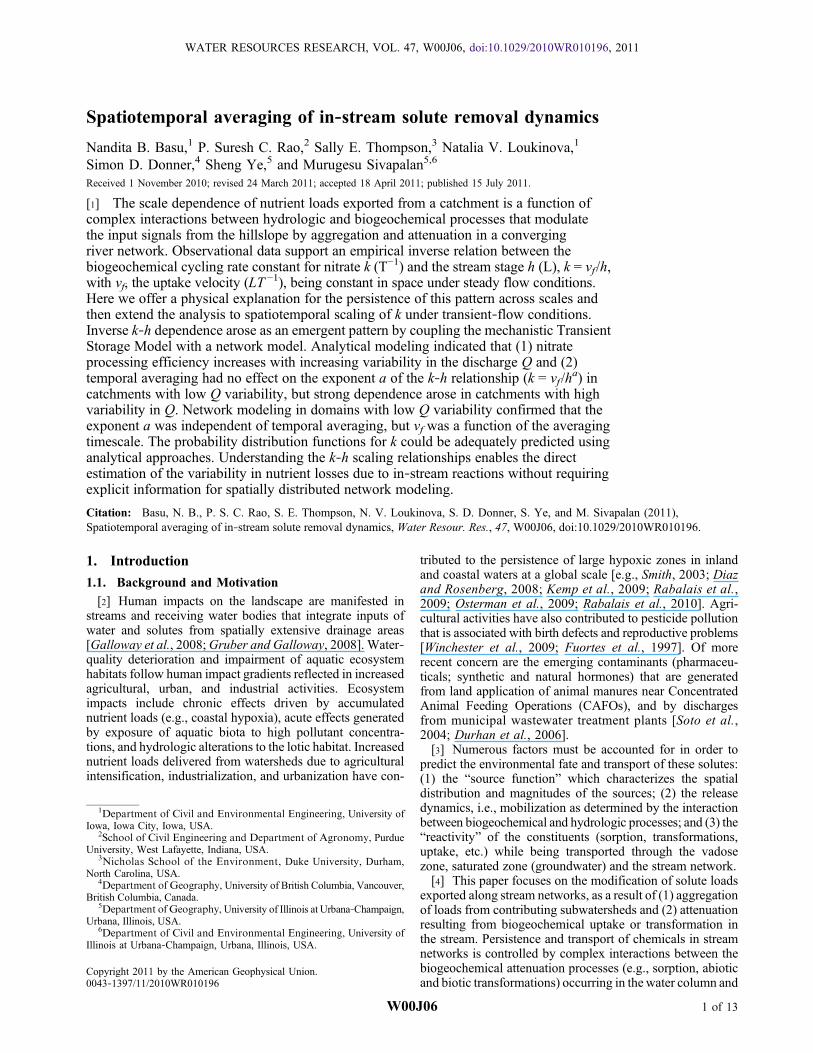
Spatiotemporal averaging of in‐stream solute removal dynamics

Nandita B. Basu,1 P. Suresh C. Rao,2 Sally E. Thompson,3 Natalia V. Loukinova,1

Simon D. Donner,4 Sheng Ye,5 and Murugesu Sivapalan5,6

Received 1 November 2010; revised 24 March 2011; accepted 18 April 2011; published 15 July 2011.

[1] The scale dependence of nutrient loads exported from a catchment is a function ofcomplex interactions between hydrologic and biogeochemical processes that modulatethe input signals from the hillslope by aggregation and attenuation in a convergingriver network. Observational data support an empirical inverse relation between thebiogeochemical cycling rate constant for nitrate k (T−1) and the stream stage h (L), k = vf /h,with vf, the uptake velocity (LT −1), being constant in space under steady flow conditions.Here we offer a physical explanation for the persistence of this pattern across scales andthen extend the analysis to spatiotemporal scaling of k under transient‐flow conditions.Inverse k‐h dependence arose as an emergent pattern by coupling the mechanistic TransientStorage Model with a network model. Analytical modeling indicated that (1) nitrateprocessing efficiency increases with increasing variability in the discharge Q and (2)temporal averaging had no effect on the exponent a of the k‐h relationship (k = vf /h

a) incatchments with low Q variability, but strong dependence arose in catchments with highvariability in Q. Network modeling in domains with low Q variability confirmed that theexponent a was independent of temporal averaging, but vf was a function of the averagingtimescale. The probability distribution functions for k could be adequately predicted usinganalytical approaches. Understanding the k‐h scaling relationships enables the directestimation of the variability in nutrient losses due to in‐stream reactions without requiringexplicit information for spatially distributed network modeling.

Citation: Basu, N. B., P. S. C. Rao, S. E. Thompson, N. V. Loukinova, S. D. Donner, S. Ye, and M. Sivapalan (2011),Spatiotemporal averaging of in‐stream solute removal dynamics, Water Resour. Res., 47, W00J06, doi:10.1029/2010WR010196.

1. Introduction

1.1. Background and Motivation

[2] Human impacts on the landscape are manifested instreams and receiving water bodies that integrate inputs ofwater and solutes from spatially extensive drainage areas[Galloway et al., 2008;Gruber and Galloway, 2008]. Water‐quality deterioration and impairment of aquatic ecosystemhabitats follow human impact gradients reflected in increasedagricultural, urban, and industrial activities. Ecosystemimpacts include chronic effects driven by accumulatednutrient loads (e.g., coastal hypoxia), acute effects generatedby exposure of aquatic biota to high pollutant concentra-tions, and hydrologic alterations to the lotic habitat. Increasednutrient loads delivered from watersheds due to agriculturalintensification, industrialization, and urbanization have con-

tributed to the persistence of large hypoxic zones in inlandand coastal waters at a global scale [e.g., Smith, 2003; Diazand Rosenberg, 2008; Kemp et al., 2009; Rabalais et al.,2009; Osterman et al., 2009; Rabalais et al., 2010]. Agri-cultural activities have also contributed to pesticide pollutionthat is associated with birth defects and reproductive problems[Winchester et al., 2009; Fuortes et al., 1997]. Of morerecent concern are the emerging contaminants (pharmaceu-ticals; synthetic and natural hormones) that are generatedfrom land application of animal manures near ConcentratedAnimal Feeding Operations (CAFOs), and by dischargesfrom municipal wastewater treatment plants [Soto et al.,2004; Durhan et al., 2006].[3] Numerous factors must be accounted for in order to

predict the environmental fate and transport of these solutes:(1) the “source function” which characterizes the spatialdistribution and magnitudes of the sources; (2) the releasedynamics, i.e., mobilization as determined by the interactionbetween biogeochemical and hydrologic processes; and (3) the“reactivity” of the constituents (sorption, transformations,uptake, etc.) while being transported through the vadosezone, saturated zone (groundwater) and the stream network.[4] This paper focuses on the modification of solute loads

exported along stream networks, as a result of (1) aggregationof loads from contributing subwatersheds and (2) attenuationresulting from biogeochemical uptake or transformation inthe stream. Persistence and transport of chemicals in streamnetworks is controlled by complex interactions between thebiogeochemical attenuation processes (e.g., sorption, abioticand biotic transformations) occurring in the water column and

1Department of Civil and Environmental Engineering, University ofIowa, Iowa City, Iowa, USA.

2School of Civil Engineering and Department of Agronomy, PurdueUniversity, West Lafayette, Indiana, USA.

3Nicholas School of the Environment, Duke University, Durham,North Carolina, USA.

4Department of Geography, University of British Columbia, Vancouver,British Columbia, Canada.

5Department ofGeography,University of Illinois at Urbana‐Champaign,Urbana, Illinois, USA.

6Department of Civil and Environmental Engineering, University ofIllinois at Urbana‐Champaign, Urbana, Illinois, USA.

Copyright 2011 by the American Geophysical Union.0043‐1397/11/2010WR010196

WATER RESOURCES RESEARCH, VOL. 47, W00J06, doi:10.1029/2010WR010196, 2011

W00J06 1 of 13

sediments, and the hydrologic transport processes (e.g., waterflow, hyporheic exchange) that propagate solute loads [Boyeret al., 2006]. A substantial body of literature on in‐streamprocessing at multiple spatiotemporal scales is available fornitrogen, and thus our framework and analyses are focusedon nitrate.

1.2. Metrics for In‐Stream Nitrate Loss

[5] Nitrate loss in streams is commonly described by an“in‐stream removal” metric, defined as a function (R) of theload exported by the stream (Fout), and the load deliveredfrom the landscape to the stream (Fin):

R ¼ 1� Φout

Φinð1Þ

R (0 < R < 1) varies with the specific temporal (e.g., daily,monthly, seasonal or annual) and spatial (e.g., reach orcatchment) scales of averaging. Normalization by input loadsin equation (1) accounts for variations in land use, so that Rprimarily represents the scaling of nitrate loads arising fromin‐stream processes.[6] Although a number of physical‐chemical processes

drive nitrate losses in streams, the cumulative effects of theseprocesses are traditionally described using first‐order kinetics[Alexander et al., 2000; Boyer et al., 2006]. At the scale of asingle reach, and assuming first‐order removal kinetics, R canbe described as a function of the first‐order biogeochemicalcycling rate constant k (T−1) and themean hydraulic residencetime within the reach t [T] (= L/u; where L is the length of thereach, and u [L/T] is the stream velocity):

R ¼ 1� exp �k�ð Þ ð2Þ

The two dominant processes that remove nitrate from streamsare biotic uptake in the water column, and denitrificationwithin the anoxic sediment [e.g., Doyle, 2005; Böhlke et al.,2008]. Of these, denitrification is the primary process con-tributing to the net removal of N within the river network[Wollheim et al., 2006; Boyer et al., 2006]. Assimilatoryprocesses (e.g., plant uptake) result in temporary removal ofnitrate, but mineralization eventually releases the nitrogenback to the water column [Wollheim et al., 2006].[7] For this study we focus on denitrification, and in the

rest of the manuscript k will be used to denote the effectiverate constant for denitrification. The parameter k representsthe combined effect of mass transfer rates across the sedi-ment‐water interface and denitrification rates in the streamsediment. Significant spatial variability has been documentedin these rates as a function of stream sediment characteristics,local gradients, availability of carbon, and redox conditions[Inwood et al., 2005; Arango et al., 2007; Arango and Tank,2008; Mulholland et al., 2008; Battin et al., 2008]. Despitethis complexity, several experimental studies conductedunder steady flow (base flow) conditions have shown that thefirst‐order denitrification rate constant varies inversely withstream stage h [L]; k = vf /h, with vf, the uptake velocity (LT

−1)being essentially constant [Alexander et al., 2000; Doyleet al., 2003; Wollheim et al., 2006; Ensign and Doyle,2006; Alexander et al., 2009; Marcé and Armengol, 2009].[8] A constant vf has been attributed to decrease in the

volume of the anoxic sediment zone relative to the water

column with increase in stream depth [Wollheim et al., 2006;Botter et al., 2010]. However, a quantitative explanation ofthe observed stage dependence of k, and an analysis of theexpected variability of vf as a function of the mass transferand the denitrification parameters is largely lacking. Theinverse stage dependence of k has interesting implicationsfor scaling of solute loads. Stream discharge and stage varyin space (along a stream network), as well as in time(transient flow in response to storm events) at any reachwithin the network, leading to spatiotemporal fluctuationsin k. While the scaling behavior of hydrologic variables(e.g., Q, h, t) along a stream network has been studiedextensively [McKerchar et al., 1998; Rodriguez‐Iturbe andRinaldo, 1997], the scaling relationships of biogeochemicalprocessing (manifested in k) have not been well explored[Alexander et al., 2000].

1.3. Objectives and Organization

[9] This paper explores the scale dependence of the bio-geochemical cycling rate constant (k; T−1) along a streamnetwork, and the relative role of hydrologic and biogeo-chemical controls on k. Three key questions drive the analysis.[10] 1. What are the underlying process level explanations

for the persistence of the observed inverse relationshipbetween k and h for nitrate attenuation dynamics in streams?[11] 2. How do reach‐scale k‐h relationships, measured

under steady‐flow conditions, vary with spatial and temporalaveraging through aggregation along a converging streamnetwork during transient‐flow conditions?[12] 3. Can the intra‐annual variability in hydroclimatic

forcing coupledwith hydrologic and biogeochemical controlsbe used to predict the intra‐annual variation in k?[13] Answering question 1 (section 4) would help to bridge

the gap between mechanistic approaches used at the reachscale and empirical approaches used at the network scale (seesection 2.2 for further details). It would also provide insightinto the expected range of vf values based on measurablestream attributes (e.g., mass transfer rate across the sedimentwater interface, and denitrification rate constant in the sedi-ment). Question 2 (section 5) has important implications forthe prediction of in‐stream solute losses due to biogeochemicalprocesses. We hypothesize that if indeed scale‐dependentrelationships emerge, predicting such losses may be possibleusing analytical approaches, avoiding the need to use spatiallydistributed stream network models. Finally, answering Ques-tion 3 (section 6)would enable the estimation of the probabilitydensity functions (pdf’s) to characterize the mean and vari-ability in nutrient removal, based only on estimates of knownclimatic and anthropogenic forcing. Before we address thesethree questions explicitly, a conceptual framework to permitanalysis of the problem is developed in section 2 and themethodology is described in section 3.

2. Conceptual Framework

2.1. Hydrologic Versus Biogeochemical Controlson Nitrate Removal Dynamics

[14] Denitrification occurs primarily in the anoxic streamsediment, which is supplied with nitrate from the water col-umn by mass transfer across the sediment‐water interface[Stream Solute Workshop, 1990]. These interactions can bequantified using the transient storage model (TSM), first

BASU ET AL.: SOLUTE REMOVAL IN STREAM NETWORKS W00J06W00J06

2 of 13

proposed by Bencala and Walters [1983], and extensivelyused since then in tracer studies in streams [Wagner andGorelick, 1986; Hart, 1995; Green et al., 1994; Runkel andChapra, 1993; Harvey et al., 1996; Marion et al., 2003,2008]. Block A in Figure 1 is a schematic representation ofthe two‐compartment TSM model that describes reach‐scaleconcentration dynamics as a function of the mass transfer rateconstant a [T−1] at the sediment‐water interface, and thedenitrification rate constant in the stream sediment ksed [T

−1].Note that ksed and a can vary spatially within a reach, and thevalues used here are average values for over reach.[15] The TSM approach described above has been exten-

sively used at the reach scale to interpret reactive and non-reactive tracer data [Mulholland and DeAngelis, 2000;Thomas et al., 2003; Tank et al., 2008]. At catchment scales,however, nitrate transport modeling is primarily based onempirical relationships (k = vf /h). The lack of a mechanisticlink between the two scales makes applying reach‐scaleexperimental data to catchment‐scale predictions challeng-ing. Botter et al. [2010] attempted to establish a link betweenreach and catchment scales by deriving a functional form forthe k‐h relationship from TSM. However, their analysis waslimited by assumptions of steady state, and specific functionalform for the mass transfer rate.[16] Here, we will expand on their work by solving the

coupled reach‐scale TSM equations under steady and tran-sient flow conditions, to estimate R and k (using equation (1))by making reasonable assumptions regarding the mean travel

time (see section 3). The k (block B in Figure 1) thus esti-mated represents the combined effects of the mechanistichydrologic (a) and biogeochemical (ksed) parameters. Eval-uating the expected range of the empirically defined kor uptake velocity (vf = kh) for measured ranges of themass transfer and denitrification parameters enables link-ing mechanistic and empirical approaches of solute removaldynamics.

2.2. Spatiotemporal Scaling of In‐Stream RemovalAlong a River Network

[17] Because k depends on h, spatiotemporal fluctuationsin flow conditions (Q or h) are propagated into k. Given thatthese Q and h fluctuations scale predictably through spaceand time [Rodriguez‐Iturbe and Rinaldo, 1997], k should alsodisplay predictable scaling behavior. Establishing such rela-tionships enable prediction of total annual in‐stream removalat the reach and network scales, without using explicit dis-tributed network models.[18] A schematic of the spatiotemporal averaging scheme

is presented in Figure 1 (blocks C and D). We start witha relationship between k and h measured under base flowscenarios (block B in Figure 1), then scale up in time (block Cin Figure 1) to obtain a relationship between kt (temporallyaveraged reaction rate constant) and hmean (hmean = meanannual (or, monthly) stage at any reach estimated from themean annual (or, monthly) discharge and the stage‐discharge

Figure 1. Schematic showing spatiotemporal averaging of reaction rate constants along the streamnetwork.

BASU ET AL.: SOLUTE REMOVAL IN STREAM NETWORKS W00J06W00J06

3 of 13

relationship), and scale up in space (block D in Figure 1) overa stream network to obtain a relationship between kst (spa-tiotemporally averaged reaction rate constant) and hmean.Note that for network‐scale analysis, hmean is the mean annualstage at the reach immediately upstream of the node at whichthe averages are estimated (i.e., a local value rather than acatchment‐scale average value). The significance of thesemean values for describing spatiotemporally averaged param-eters will be discussed below.[19] The temporally and spatiotemporally averaged reac-

tion rate constants kt [T−1] and kst [T

−1], respectively, aredefined as

kt ¼ Ln 1� Rtð Þ�t

ð3Þ

kst ¼ Ln 1� Rstð Þ�st

ð4Þ

whereRt andRst are the fractional nutrient removal, as definedin equation (2), with the subscript t denoting the specifiedaveraging timescale (here we use annual or monthly) for agiven stream reach, and subscript st denoting averaging overall reaches upstream of a node in the network. In addition,tt and tst are the temporally and spatiotemporally averagedresidence times, respectively. Scaling of k to estimate ktand kst requires an understanding of how to scale nutrientremoval (R) and the residence time t; this is accomplishedusing the results of a network model (section 5).

2.3. Probability Distribution Functions for k

[20] The intra‐annual variability in k (as described by itspdf, p(k)) has received considerably less attention thandescriptions of mean behavior [Doyle, 2005; Marcé andArmengol, 2009; Hoellein et al., 2007; Böhlke et al., 2008;Botter et al., 2010]. Intra‐annual variability of streamhydrologic conditions (e.g., frequency, duration and magni-tude of the stream discharge) are directly controlled by thestochastic nature of the hydroclimatic forcing (rainfall pat-terns, potential evapotranspiration demands), and the spatialdistribution of landscape attributes (soils, topography, vege-tation) [Botter et al., 2007a, 2007b, 2008, 2010]. The sto-chasticity in Q means that the stream depth (h) and the

removal rate constant (k) are also random variables [Botteret al., 2007a, 2007b, 2008, 2010]. Botter et al. [2010]examined the stochastic properties of the intra‐annual varia-tions in k in a stream reach, by linking rainfall forcing,landscape features, and stream geomorphology to in‐streamprocesses. Assuming the streamflow pdf, p(Q), to be aGamma function, a power law relationship between stage anddischarge (h = mQn; m and n are constants), and an inversestage dependence of k, Botter et al. [2010] developed thefollowing analytical expressions for the pdf of the streamstage, p(h) and nutrient removal rate constant p(k):

p Qð Þ ¼ ��=kcQ Q�=kc�1 exp ��QQ

� �G �=kcð Þ ð5Þ

p kð Þ ¼W Wkð Þ � �

nkc�1ð Þexp � Wkð Þ�1=n

� �G �=kcð Þn ð6Þ

where l [T−1] = frequency of streamflow producing rainfallevents; kc [T

−1] = inverse of mean catchment residence time;gQ [T/L3] is the mean runoff; and G(l/kc) is the completeGamma function of the argument l/kc; Ω = 1/(�vf); � = gQ

n /mrepresents the inverse of the stage observed when the dis-charge is equal to the mean streamflow jump produced by therunoff events. The analytical equations developed by Botteret al. [2010] will be evaluated using results from the net-work model (section 6).

3. Methods

[21] Methods of analysis specific to the three key questions(see section 1.3) are presented below; overlap of methodsbetween these questions was necessary to maintain clarity.

3.1. Mechanistic Basis for the Empirical k‐hRelationship (Question 1)

[22] We used a dynamic network flowmodel, coupled witha two compartment (sediment and water) biogeochemicalprocess model. The dynamic network flow model is basedon the representative elementary watershed (REW) theory ofReggiani et al. [1998, 1999, 2001], while the biogeochemicalprocess model is based on the upscaling of the TSM modelequations for dissolved nutrients [Bencala and Walters,1983; Runkel, 1998], with explicit inclusion of the interac-tions between the main water column and the sediment zone(S. T. P. Ye et al., Dissolved nutrient removal dynamics inriver networks: A modeling investigation of transient flowsand scale effects, submitted to Water Resources Research,2011). The TSM equations are solved at the reach scale wherethe advection term and the lateral mass inflow term arereplaced by solute mass input from upstream nodes, and massoutput to downstream nodes. We thus neglect longitudinalvariations within a reach, but consider this approximationto be reasonable since our interest lies at the network scale.The coupled model is implemented using a river networkextracted from the digital elevation model available for LittleVermilion River Watershed, (LVRW) a 489 km2 basin(Figure 2) in east central Illinois [Mitchell et al., 2000;Algoazany, 2006]. Further details of themodel and the site arepresented by Ye et al. (submitted manuscript, 2011).

Figure 2. Map of the Little Vermilion River Basin in eastcentral Illinois with 29 REWs delineated.

BASU ET AL.: SOLUTE REMOVAL IN STREAM NETWORKS W00J06W00J06

4 of 13

[23] Model outputs were used to analyze the effects of themass transfer rate constant a (T−1), and the removal rateconstant in the stream sediment ksed (T

−1) on the resultant k‐hrelationship. We first explored this question under steadybase flow (1 mm/d) conditions. The steady‐flow simulationswere expected to mimic the steady state stream tracerexperiments that are the source of most of the available data,and simplify the system dynamics by omitting flood wavepropagation. A constant input nitrate concentration of 5 mg/Lwas used to simulate typical ranges of nitrate concentration atbase flow in the watersheds dominated by corn‐soybeanrotations in the Midwestern United States. [Schilling andLibra, 2000]. Note that given the assumption of linear reac-tion kinetics for denitrification, the choice of nitrate con-centration has no effect on the first‐order rate constant. Thereach‐scale removal Rwas estimated as the ratio of the solutemass lost in the reach and the mass delivered to that reach.The residence time (t) was calculated using the reach lengthand Manning’s equation for velocity. The rate constant k wasestimated using equation (2), and expressed as k = vf /h

a.Instead of implicitly assuming an empirical form of vf (= kh)[Wollheim et al., 2006], we analyzed the simulation outputs todetermine the vf and a values that were the best fit to themodel outputs. The variability in vf and a was evaluated asa function of variations in a and ksed for which a reasonablerange of empirical values were obtained from the literature,as discussed below.[24] Battin et al. [2008] provide a compilation of a (T−1)

values estimated in reach‐scale tracer experiments in tem-perate, tropical, semiarid and Arctic streams (Figure 3, left).Across these diverse sites, a values follow an asymmetricdistribution (range: 0.02–16 h−1) with a modal value of0.36 h−1, and 80% of the values between 0.02 and 2 h−1.Estimates of the reach‐scale mean rate constant in the sedi-ment ksed (T

−1) are sparse in comparison to a. Most streamnutrient studies are focused on estimating the effective lossrate between two sampling locations, which provides anestimate of k, not ksed. Our estimates of the behavior of ksedare therefore based on a single large‐scale nitrogen stableisotope study, the Lotic Intersite Nitrogen Experiment(LINX). LINX examined 72 representative reaches in NorthAmerica to investigate in‐stream N retention processesunder base flow conditions [Mulholland et al., 2008]. Theestimated k values followed a strongly asymmetric distribu-tion (Figure 3, right), with a range between 0.002 to 4.8 h−1,and a mode of 0.01 h−1; 80% of the values were between0.002 and 0.08 h−1. For our analysis, we useda = 0.025, 0.25,

1 and 2.5 h−1 and ksed = 0.025, 0.1, 0.5 and 2.5 h−1 to cover the

range of values reported in the literature.

3.2. The k‐h Scale Dependence (Question 2)

[25] We explored this question using models of varyinglevels of complexity: (1) analytical approach at the reachscale for the kt‐hmean relationship, (2) mechanistic approachincluding Transient Network Simulations (TSM+REW) forkt‐hmean and kst‐hmean relationship, and (3) network modelingof the Mississippi‐Atchafalaya River Basin (MARB) for thekst‐hmean relationship. The three modeling approaches haddifferent assumptions as discussed below. The convergencebetween these varying approaches suggests that the resultsare robust against variations in model assumptions and lim-itations. Experimental data to explore scale dependence ofin‐stream solute losses are largely lacking at the networkscale, which forces this strong dependence on modelinganalyses to draw inference at these scales.[26] The analytical approach is based on using the pdf ofQ

(as defined by stochastic hydroclimatic controls) and thedependence of k and t on Q to estimate the temporallyaveraged rate constant kt at the reach scale. To do so we useequation (3) and the following definitions of Rt and tt:

Rt ¼Z

p Qð ÞR Qð ÞdQ ¼Z

p Qð Þ 1� exp �k�ð Þð ÞdQ

¼Z

p Qð Þ 1� exp � vfh

L

u

� �� �dQ ð7Þ

�t ¼Z

p Qð Þ� Qð ÞdQ ¼Z

p Qð Þ L

u

� �dQ ð8Þ

[27] Here, power function relationships between h andQ (h = mQn; m and n are constants) and u and Q (u = rQs;r and s are constants) are used to describe the dependence ofR and t on the stream hydraulic variables. We assumed aGamma distribution to describe p(Q) (equation (5)) and cal-culated the mean stage hmean using the mean discharge Qmean

and the stage‐discharge relationship. The tractability of theanalytical approach enabled an explicit comparison of thekt‐hmean relationship across different catchment‐climateregimes (as embodied in l/kc), as well as biogeochemicalregimes (as embodied in vf). Five values of l/kc = 0.5, 1, 1.5,2 and 2.5 were used, representing a progression of decreas-ing variability in the streamflow distribution. Increases in

Figure 3. Distribution of experimental values for (left) the mass transfer exchange rate a and (right) therate of denitrification in stream sediments (ksed) [Battin et al., 2008; Mulholland et al., 2008].

BASU ET AL.: SOLUTE REMOVAL IN STREAM NETWORKS W00J06W00J06

5 of 13

l/kc correspond to a decrease in the variability of p(Q)(equation (5)), since the coefficient of variation of the Qdistribution is given by

ffiffiffiffiffiffiffiffiffikc=�

p. Two uptake velocities vf = 10

and 100 m/yr were used, based on a range of values drawnfrom data synthesis [Wollheim et al., 2006]. Note that theserates represent removal by denitrification only, and aresmaller than reported uptake velocities when both denitrifi-cation and biotic uptake within the water column are con-sidered [Doyle, 2005]. Finally, we used m and n values of0.3 and 0.4, and r and s values of 0.3 and 0.2 based on theaverage (over all reaches) scaling behavior predicted bythe hydraulic model (REW) mentioned in section 3.1 anddescribed in Ye et al. (submitted manuscript, 2011).[28] The analytical approach is easily tractable, but

required several simplifying assumptions that were relaxed inthe two network numerical modeling approaches (approachesb and c; see above). The two network approaches were dis-tinctly different in their model assumptions, as well as thescale of analysis. The mechanistic approach (approach b), asdescribed in section 3.1, used the two‐compartment TSMapproach coupled to a dynamic flow model to describe thedenitrification kinetics. The kt‐hmean and kst‐hmean relation-ships were estimated as functions of nested scales (2 km2 –489 km2) in a single watershed, and for a single climaticregime representative of the humid Midwest United States.The empirical modeling (approach c), was done as a part of aseparate study, and used the coupled IBIS‐THMB Model[Donner et al., 2002, 2004]. IBIS‐THMB employs standardempirical approaches (k = vf /h) to describe denitrificationkinetics. The kst‐hmean relationship was estimated at the outletof large watersheds (>10,000 km2; see Table 1 for details onindividual watersheds), across different climatic regimes inthe MARB system. The scale of resolution (∼ 100 km2) wasmuch coarser in the MARB study making nested analysissimilar to LVRW difficult. Variable discharge and concen-tration time series data from subwatersheds were used asinputs to the stream network model in both approaches. InLVRW, the model was run for 7 years, while in MARB theduration of the model run was 30 years.[29] The reach‐ and network‐scale effective rate constants

(kt and kst) were calculated using equations (3) and (4), modeloutputs of Rt and Rst, and estimates of tt and tst. The tem-porally averaged residence time was calculated in approach bbased on Manning’s equation for velocity and the length ofthe reach. The spatiotemporally averaged residence time tst inapproach b was estimated by considering the distribution oftravel paths to a node, and the mean travel times along those

paths (Ye et al., submitted manuscript, 2011). The spatio-temporally averaged residence time tst in approach c wasbased on simple scaling relationships that exist between res-idence times and upstream contributing area (t = −0.0065 +0.2642A1/3, t is the residence time in days and A is theupstream contributing area in km2 [Alexander et al., 2000]).

3.3. The Probability Distribution Function of k(Question 3)

[30] Botter et al. [2010] developed an analytical expressionto describe the intra‐annual probability distribution functionof k as a function of underlying climatic, hydrologic andbiogeochemical controls (see equation (5)). The outputs fromthe MARB analysis were used to explore the predictivecapacity of this analytical approach (section 6). The distri-bution of kst values estimated using Rst and tst in the MARBanalysis were used to plot the intra‐annual pdf of k. Toevaluate the predictive capacity of the analytical approach,we fitted the monthly discharge data to gamma distributions,and estimated gQ and l/kc (Table 1). The estimated gQ andl/kc, and the mean exponent and coefficient of the monthlykst‐hmean relationship were then used to predict the pdf of k.

4. Mechanistic Basis for the Empirical k‐hRelationship

[31] Process level controls on the experimentally observedk‐h relationship were investigated by coupling a reach‐scalemechanistic model with a spatially explicit network model.The statistical distributions for a and ksed derived from theliterature were asymmetric (Figure 3), prompting us to selectthe mode value (a = 0.36 h−1; ksed = 0.01 h−1) for modelsimulations. The reach‐scale removal is presented as functionof increasing discharge for first‐, second‐ and third‐orderstreams along the river network in LVRW (Figure 4). Asexpected, R decreases with increase in Q because the sedi-ment‐water contact area is proportionally smaller, resultingin smaller in‐stream losses (Figure 4). Methods outlined insection 3.1 were used to estimate k from R (Figure 5). Wefound the k‐Q relationship to be well described by a powerfunction (k = 1.97Q−0.44; R2 = 0.91). Further, for this network,the imposed hydraulics dictated the existence of a power‐function relationship between reach‐scale h (m) andQ (m3/s)

Table 1. Parameters of the Probability Distribution Function of k(Figure 11) for Watersheds in the Mississippi Basin [Donner et al.,2004]

Watershed NameArea(km2)

Predicted Fitted

l/kc1/gQ(m3/s) l/kc

1/gQ(m3/s)

Allegheny 29,098 2.8 183 0.6 2,415Muskinghum 16,000 1.9 97 4.0 63Rock 23,766 2.6 101 0.7 1,085Iowa 32,224 2.2 150 0.8 6,89Illinois 71,606 2.9 276 0.8 1,790Tennessee 143,373 1.6 1,528 1.1 2,931Yellowstone 179,341 2.7 96 1.5 137Grand 19,878 2.0 88 0.8 441Canadian 75,669 2.6 41 1.0 67

Figure 4. Relationship between reach scale R and Q for dif-ferent stream orders. Simulation results are based on the net-work model in the Little Vermilion River Watershed.

BASU ET AL.: SOLUTE REMOVAL IN STREAM NETWORKS W00J06W00J06

6 of 13

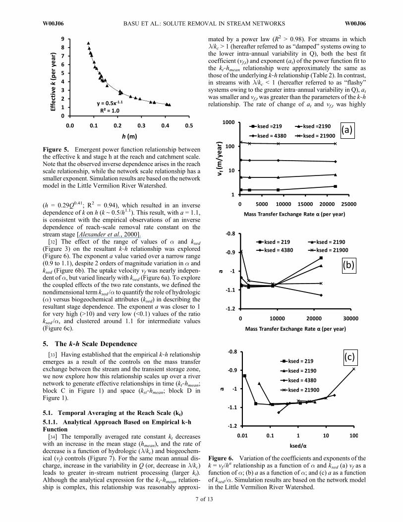
(h = 0.29Q0.41; R2 = 0.94), which resulted in an inversedependence of k on h (k ∼ 0.5/h1.1). This result, with a = 1.1,is consistent with the empirical observations of an inversedependence of reach‐scale removal rate constant on thestream stage [Alexander et al., 2000].[32] The effect of the range of values of a and ksed

(Figure 3) on the resultant k‐h relationship was explored(Figure 6). The exponent a value varied over a narrow range(0.9 to 1.1), despite 2 orders of magnitude variation in a andksed (Figure 6b). The uptake velocity vf was nearly indepen-dent of a, but varied linearly with ksed (Figure 6a). To explorethe coupled effects of the two rate constants, we defined thenondimensional term ksed /a to quantify the role of hydrologic(a) versus biogeochemical attributes (ksed) in describing theresultant stage dependence. The exponent a was closer to 1for very high (>10) and very low (<0.1) values of the ratioksed /a, and clustered around 1.1 for intermediate values(Figure 6c).

5. The k‐h Scale Dependence

[33] Having established that the empirical k‐h relationshipemerges as a result of the controls on the mass transferexchange between the stream and the transient storage zone,we now explore how this relationship scales up over a rivernetwork to generate effective relationships in time (kt‐hmean;block C in Figure 1) and space (kst‐hmean; block D inFigure 1).

5.1. Temporal Averaging at the Reach Scale (kt)

5.1.1. Analytical Approach Based on Empirical k‐hFunction[34] The temporally averaged rate constant kt decreases

with an increase in the mean stage (hmean), and the rate ofdecrease is a function of hydrologic (l/kc) and biogeochem-ical (vf) controls (Figure 7). For the same mean annual dis-charge, increase in the variability in Q (or, decrease in l/kc)leads to greater in‐stream nutrient processing (larger kt).Although the analytical expression for the kt‐hmean relation-ship is complex, this relationship was reasonably approxi-

mated by a power law (R2 > 0.98). For streams in whichl/kc > 1 (hereafter referred to as “damped” systems owing tothe lower intra‐annual variability in Q), both the best fitcoefficient (vf,t) and exponent (at) of the power function fit tothe kt‐hmean relationship were approximately the same asthose of the underlying k‐h relationship (Table 2). In contrast,in streams with l/kc < 1 (hereafter referred to as “flashy”systems owing to the greater intra‐annual variability in Q), atwas smaller and vf,twas greater than the parameters of the k‐hrelationship. The rate of change of at and vf,t was highly

Figure 5. Emergent power function relationship betweenthe effective k and stage h at the reach and catchment scale.Note that the observed inverse dependence arises in the reachscale relationship, while the network scale relationship has asmaller exponent. Simulation results are based on the networkmodel in the Little Vermilion River Watershed.

Figure 6. Variation of the coefficients and exponents of thek = vf /h

a relationship as a function of a and ksed (a) vf as afunction of a; (b) a as a function of a; and (c) a as a functionof ksed /a. Simulation results are based on the network modelin the Little Vermilion River Watershed.

BASU ET AL.: SOLUTE REMOVAL IN STREAM NETWORKS W00J06W00J06

7 of 13

nonlinear (Table 2) and greater for the smaller vf (=10 m/yr).These results indicate the emergence of scale independencein “damped” streams, while strong nonlinearity and scaledependence might be more characteristic of “flashy” streams.This arises due to the strong asymmetry in p(Q) in flashystreams that leads to hmean not being the representative stage.5.1.2. Mechanistic Approach (TSM+REW)[35] The reach‐scale kt‐hmean relationship (Figure 8a) for

different reaches along the stream network in LVRW wasestimated using outputs from the mechanistic network model(TSM + REW) and the methods outlined in section 3.2. Withincreasing contributing area along the nodes of the network,hmean increases, resulting in a decrease in kt. We compareresults obtained under steady‐flow scenarios with transient‐flow simulations using monthly and annual averaging. Forboth the monthly and annual averaging, all 7 years of datacollapsed to yield a unique kt‐hmean power‐function rela-tionship (Figure 8a). The exponent of the relationship wassimilar for both averaging time scales and equal to theexponent of the steady‐flow relationship, suggesting emer-gence of temporal‐scale invariance. The coefficient (vf,t) wassimilar for the steady flow and the monthly averaging sce-narios, but lower for the annual averaging scenario. This

difference is attributed to the carryover of residual nitrate inthe stream sediments across averaging periods, as discussedbelow.[36] Carryover refers to the fraction of the nitrate that is

retained in the system (particularly in stream sediments)between averaging periods. It arises from the residence timeof some of the nitrate being greater than the averaging time-scale. We found significant carryover of nitrate both in thesteady and the transient flow simulations, especially at annualtime scales. This led to the total nitrate removal being greaterthan the nitrate input into the stream network for some years.While carryover between adjacent time periods is plausible,observations of removals exceeding inputs are anomalousfrom amass balance perspective. To correct for this effect, weinitialized the model at the start of every year to run withzero nitrate in the sediment. We attribute the lower vf,t at the

Figure 7. Analytical modeling used to derive the kt‐hmeanrelationship for l/kc = 0.5, 1, 1.5, 2, and 2.5 and vf = 10 m/yr(dashed lines) and 100 m/yr (solid lines). Power functionsare fitted to the kt‐hmean relationship, and the resulting expo-nents and coefficients are presented in Table 2. Results showthat the k‐h relationship does not change with temporalaveraging in wet (l/kc > 1) domains but is significantlyaffected by averaging in dry domains (l/kc < 1).

Table 2. Exponents (at) and Coefficients (vf,t) of the Power‐Function Fit to the kt‐hmean Relationship Function of TemporalAveraging Using the Analytical Approach

l/kc

at vf,t

vf = 10 vf = 100 vf = 10 vf = 100

0.5 0.63 0.59 46 2741.0 0.95 0.90 18 1831.5 0.98 0.98 9 912.0 1.00 1.00 9 912.5 1.00 1.00 9 91

Figure 8. Relationship between the effective k and meanstage at (a) the reach scale and (b) the catchment scale. Sim-ulation results are based on the network model in the LittleVermilion River Watershed. Black triangles represent thebase flow scenario, black crosses represent monthly outputsfrom the transient simulations, and colored symbols representannual outputs from the transient simulations. Each colorindicates a different year, while each data point indicates adifferent reach for reach scale analysis and a different nodein the network for catchment scale analysis.

BASU ET AL.: SOLUTE REMOVAL IN STREAM NETWORKS W00J06W00J06

8 of 13

annual time scale as being due to this initialization. A lowercoefficient indicates that there was less removal at the annualtime scale than at monthly scales, which occurs because weneglect the effect of potential removal of the carryover nitratefrom the previous year. There is little data on carryover in thefield because most reach‐scale studies are short‐durationexperiments. Previous modeling studies did not encounter thecarryover effect since they were based on empirical functionsfor nitrate removal in the stream sediment. Our results indi-cate that carryover does not affect the exponent of the k‐hrelationship, but does affect the magnitude of the uptakevelocity. Sensitivity of the uptake velocity to the carryoverfraction, and existence of carryover in field studies need tobe explored in further detail in future work.

5.2. Spatiotemporal Averaging at the Network Scale

5.2.1. Mechanistic Approach (Based on TSM+REW)[37] The network‐scale kst‐hmean relationship (Figure 8b)

along the LVRW stream network is estimated using outputsfrom the mechanistic network model (TSM + REW) and themethods outlined in section 3.2.We compare results obtainedunder steady‐flow scenario with transient‐flow simulationsusing monthly and annual averaging (Figure 8b). The expo-nent of the kst‐hmean relationship was similar betweensteady‐ and transient‐flow simulations, but lower than theexponent of the kt‐hmean. The smaller value of the exponent ofthe kst‐hmean relationship compared to the kt‐hmean relation-ship is attributed to the greater processing that occurs at thenetwork scale because of the longer residence time. Similar tothe observations for temporal averaging, vf,t values weresimilar for monthly averaging and steady‐flow scenarios,but lower for annual averaging. We attribute this effectto carryover of residual nitrate, as discussed in section 5.1.2.5.2.2. Empirical Approach (Based on Donner et al.[2004])[38] Donner et al. [2004] presented the results from basin‐

scale simulations for percent annual in‐stream removal ofnitrate as a function of basin‐averaged precipitation (P). Theynoted an inverse relationship between nitrogen removal andincreasing precipitation (Figure 9a). Despite the presence ofthis general pattern of inverse dependence across watershedsin different climatic regimes, the specific R‐P relationshipappeared to be watershed specific, with similar precipitation

leading to different removal fractions in different watersheds.In contrast to basin specific patterns of R‐P, the kst‐Qmean

relationship for all nine watersheds collapsed to yield a singlepower function with an exponent of 0.42 (Figure 9b). Thiscollapse of seemingly diverse watershed nitrate removalbehaviors in large basins across a range of climatic types, togenerate a single effective kst‐Qmean relationship is striking,and indicates that it might be possible to estimate basin‐scalein‐stream nutrient losses without explicit spatial networkanalysis. It also implies that hydrologic filtering (the con-version of precipitation to streamflow by filtering through thelandscape) governed the variability in nutrient removal acrosswatersheds.[39] The corresponding kst‐hmean relationship, plotted

using a stage discharge relationship h = 0.26Q0.4 (based on astudy of 112 river locations in the United States, Leopold andMaddock [1953]), yielded an approximate inverse stagedependence (Figure 10). Consistent with our previous obser-vation (approach b), the exponent of the kst‐hmean relationshipwas independent of the averaging timescale, but the coefficientvaried with averaging (Figure 10). In contrast to the mecha-nistic approach (approach b) described before, the coefficienthere is greater at the annual time scale than the monthly timescale. Themechanistic approach had the carryover effect that isabsent in the empirical approach used byDonner et al. [2004].Here, the differences in the coefficients at the two averagingtime scales arise from the assumption of hmean being the rep-resentative stage. The total annual removal at any node in awatershed is the sum of removal through all pathways (from allfirst‐order subwatersheds) leading to that node. During travelthrough any of these pathways, channels of increasing depthand decreasing removal efficiency is encountered. It is intui-tively obvious that the representative stage would be lowerthan the mean stage at the outlet, which is the largest stageencountered along any of the pathways from source to outlet. Arepresentative stage at the watershed scale will be a functionof the hydroclimatic controls, and the network topology andgeomorphology that defines the distribution of stage through-out the network. However, the exact functional relationshipbetween the mean stage at the outlet and the spatiotemporaldistribution of stages requires further analyses and is beyondthe scope of this work.

Figure 9. Mississippi Basin simulations by Donner et al. [2004]: (a) in‐stream removal decreases withincrease in precipitation and (b) collapse of all basins to yield a single relationship between effective k andQ.

BASU ET AL.: SOLUTE REMOVAL IN STREAM NETWORKS W00J06W00J06

9 of 13

6. Probability Distribution Function of k

[40] Having explored basin‐wide scaling of k using semi-empirical models and uncovering a remarkably convergentbehavior at monthly and annual averaging timescales, wenext explored if the intra‐annual pdf of k could be predictedas a function of the underlying climate, hydrologic and geo-

morphic controls in the system. As proposed by Botter et al.[2010], the pdf of k can be described by a Gamma distri-bution using parameters of p(Q) and the k‐Q relationship(equations (5) and (6)). The discharge pdf’s could bedescribed well by gamma distributions with l/kc rangingbetween 2 and 2.4 (Table 1). These parameters were able toreasonably capture the intra‐annual pdf of k using the sto-chastic model proposed by Botter et al. [2010] (Figure 11).Of the nine basins explored in this study, the Botter et al.[2010] approach predicted the pdf’s for some basins betterthan others. However, no definite correlation could beestablished between the distribution of Q and the predictiveability of the stochastic model. In addition to prediction, wefitted the pdf of k which as expected describes the numericalresults better (Figure 11).

7. Discussion

7.1. Persistence of the Inverse Stage Dependence of k

[41] We investigated process controls on the experimen-tally observed inverse stage dependence of the denitrificationrate constant k. Our results showed that over 2 orders ofmagnitude variation in the mass transfer exchange rate (a)and the sediment denitrification rate constant (ksed), theexponent, a, of h in the k = vf /h

a relationship varied onlybetween 0.9 and 1.1, thus validating the empirical results thatassume a ∼ 1. The inverse relationship was robust andinsensitive to wide range of variations in two key sedimentcharacteristics:a and ksed. The robustness of the relationship isattributed to the mass transfer constraints to hyporheic

Figure 10. Relationship between the effective kst and hmeanat annual (triangles) and monthly timescales (crosses). Resultsare based on Mississippi Basin simulations by Donner et al.[2004].

Figure 11. Probability distribution functions of the first‐order effective rate constant for nine large basinsin MARB. Histograms indicate simulation results from Donner et al. [2004], the red line is the predicteddistribution from Botter et al. [2010], and the green line is the fitted distribution.

BASU ET AL.: SOLUTE REMOVAL IN STREAM NETWORKS W00J06W00J06

10 of 13

exchange being the rate‐limiting step for removal, such that thesystem becomes comparatively insensitive to local biogeo-chemical attributes. The TSM approach explicitly accounts forthe reduction in the proportion of the anoxic zone relative to thewater column (which determines the mass transfer conditions)by simulating the flow dynamics in the channel cross section.The observation that varying a and ksed had minimal effect onthe k‐h dependence quantitatively supports the hypothesis thathe dynamics of change in contact volume (as manifested instage) leads to the persistence of the inverse relationship.[42] We further evaluated the sensitivity of the empirical

uptake velocity vf to the measured mass transfer and denitri-fication parameters. Estimated uptake velocities from ourmodel results ranged between 2 and 200m/yr, while observedvf values across MARB have been observed to be fairlyconsistent at ∼ 60 m/yr [Wollheim et al., 2006]. Our modelingresults indicated that vf was insensitive to a, but increasedlinearly with increase in ksed. The observed constant value ofvf [cf. Wollheim et al., 2006] thus suggests a fairly constantsediment denitrification rate constant ksed across systems.While this is an interesting observation, it needs to beevaluated further using reach‐scale measurements of ksed,a and vf.[43] The variability in a and ksed values represent fluvial

systems with varying hydrologic, geomorphic, and biogeo-chemical attributes. Large a value may be representative ofsandy gravelly sediments, while small a values are typical of“muddy” sediments. Sediment and soil organic carbon con-tent (OC) variations exert dominant control on ksed [e.g.,Reddy et al., 1982; Reddy and DeLaune, 2008]. Thus, largeksed values are representative of sediments with high OC, andlow dissolved oxygen that are typical of “impacted” streamsdraining agricultural lands [Inwood et al., 2005;Arango et al.,2007; Arango and Tank, 2008]. Small ksed values, on theother hand, maybe representative of sandy and gravellysediments with low OC typical of “pristine” streams. Despitesuch large variability in stream characteristics, the conver-gence to a robust, inverse stage dependence provides acompelling argument that hydrologic controls dominate overlocal‐scale sediment biogeochemical attributes.

7.2. Scaling of k‐h Relationship for the River Network

[44] The motivation of this exploration was to understandhow the local k‐h relationship, observed in stream tracerexperiments under steady flow conditions, scales up in time(kt‐hmean relationship; block C, Figure 1) and space (kst‐hmeanrelationship; block D, Figure 1). There was a surprisingconsistency in both the spatial and temporal scaling of localk‐h dynamics in the stream network.[45] Analytical modeling indicated that for the same mean

annual discharge, there is more processing (higher kt) in“flashy” streams (l/kc < 1) with high variability in Q than in“damped” streams (l/kc > 1) with low variability inQ. This isbecause in amore variable or “flashy” system, high‐dischargeevents, characterized by less in‐stream processing, are rareand of short duration, and as such they do not contribute muchto the overall reduction in nutrient removal. If these high Qvalues are distributed more uniformly over the year in a“damped” system, the stage is consistently high leading tolow removal. Our results also suggest that the intra‐annualpdf of Q had no effect on the mean annual removal in“damped” streams, and the temporally averaged kt‐hmean

relationship collapses to the underlying k‐h relationship. Incontrast, in “flashy” streams, the intra‐annual pdf of Q sig-nificantly affects the mean annual removal. In such systems,the temporally averaged kt‐hmean relationship is differentfrom the underlying k‐h relationship, with the differencebetween the two functions increasing nonlinearly withdecrease in l/kc. Thus, in “damped” systems the mean annualremoval can be estimated based solely on the mean stage andthe underlying k‐h relationship, making predictions easier.In “flashy” streams additional information is required on theintra‐annual pdf of Q which affects the kt‐hmean relationship.[46] The network models we used to further explore the

scaling question were restricted to domains with low intra‐annual variability in Q (l/kc > 1). Consistent with the ana-lytical study, the network model indicated that the exponentof the k‐h relationship was independent of spatial and tem-poral averaging scales. Scale dependence was, however,observed in the coefficient, a, of the k‐h relationship.We offer preliminary explanations for this observation insection 5, but recognize this as an area of future study. Therelatively constant a value with spatial and temporal aver-aging is intuitively obvious since we are starting with a powerfunction relationship and scaling it up over a fractal rivernetwork. If we started with other functional forms between kand h (e.g., exponential), the functional form of the relation-ship would change with spatiotemporal averaging. The con-sistencywithwhich the relationship scales up is promising andindicates that it might be possible to estimate in‐streamremoval without spatially distributed network analysis.

7.3. Prediction of Interannual Variability of k

[47] The analytical model proposed by Botter et al. [2010]adequately described the intra‐annual pdf of k produced fromreanalysis of the MARB simulations generated by Donneret al. [2004]. The ability of the stochastic approach to cap-ture the intra‐annual pdf of k that is generated using a spatiallyexplicit network model at such large scales (>10,000 km2) isencouraging, even if the predictions were not exact.

7.4. Implications and Further Work

[48] The biogeochemical scaling of solute removal instreams is interesting and consistent with similar scalingobserved for hydrologic attributes.. The results imply thatin‐stream removal can be described adequately using sim-ple scaling relationships, and without requiring a spatiallyexplicit network model. However, our conclusions are basedon comparisons with outputs from network models, and notmeasured data. This is because of a lack of network‐scale datafor evaluating nitrogen removal dynamics. Almost all of thedata available are at the scale of a single reach, making pro-jections at the network scale entirely model‐dependent. Toovercome this, in‐stream removal data at nested locationswithin stream networks at different times need to be gathered.The modeling was restricted to streams with low intra‐annualvariability in Q. We recognize the need for more carefulanalysis in networks with high Q variability; however, otherissues (e.g., temperature effects, ephemeral streams) need tobe considered in such analysis.[49] Our analysis is based on a two‐compartment model

with a hyporheic transient storage zone while recent studieshave shown [Briggs et al., 2010; Marion et al., 2008] that athree‐compartment model with an additional transient storage

BASU ET AL.: SOLUTE REMOVAL IN STREAM NETWORKS W00J06W00J06

11 of 13

zone in the water column captures the dynamics of in‐streamremoval better. However, as noted by Stewart et al. [2011],the hyporheic transient storage zone has greater influenceon nutrient removal than the surface transient storage zonebecause of longer residence times. The surface transientstorage zone is more critical for plant uptake while our focuswas on denitrification. Scaling relationships for N uptake byplants is also of interest; however, such studies would have toconsider additional factors like timescales of recycling versustimescale of averaging, as well as how uptake changes alonga river network. Finally, though we have focused on nitratefor this manuscript, similar analyses can be developed for anyreactive solute based on solute‐specific reactivity and the siteof occurrence of the reaction (e.g., within channel or in thesediment).

[50] Acknowledgments. The contributions of Nandita Basu andNatalia Loukinova were supported by the University of Iowa, while the con-tributions of Suresh Rao were supported by the Lee A. Reith Endowment andPurdue University.Work on this paper commenced during the Summer Insti-tute organized at the University of British Columbia during June–July 2009as part of the NSF‐funded project: Water Cycle Dynamics in a ChangingEnvironment: Advancing Hydrologic Science through Synthesis (NSF grantEAR‐0636043, M. Sivapalan, PI). We acknowledge the support and adviceof numerous participants at the Summer Institute. Logistic and intellectualsupport provided by the host for the Summer Institute, Marwan Hassan atUniversity of British Columbia, Canada, is much appreciated.

ReferencesAlexander, R. B., R. A. Smith, and G. E. Schwarz (2000), Effect of stream

channel size on the delivery of nitrogen to the Gulf of Mexico, Nature,403, 758–761, doi:10.1038/35001562.

Alexander, R. B., J. K. Böhlke, E. W. Boyer, M. B. David, J. W. Harvey,P. J. Mulholland, S. P. Seitzinger, C. R. Tobias, C. Tonitto, and W. M.Wollheim (2009), Dynamic modeling of nitrogen losses in river net-works unravels the coupled effects of hydrological and biogeochemicalprocesses, Biogeochemistry, 93, 91–116, doi:10.1007/s10533-008-9274-8.

Algoazany, A. S. (2006), Long‐term effects of agricultural chemicals andmanagement practices on water quality in a subsurface drained water-shed, Ph.D. thesis, Univ. of Ill. at Urbana‐Champaign, Urbana.

Arango, C. P., and J. L. Tank (2008), Land use influences the spatiotempo-ral controls on nitrification and denitrification in headwater streams, J. N.Am. Benthol. Soc., 27, 90–107, doi:10.1899/07-024.1.

Arango, C. P., J. L. Tank, J. L. Schaller, T. V. Royer, M. J. Bernot, andM. B. David (2007), Benthic organic carbon influences denitrifica-tion in streams with high nitrate concentration, Freshwater Biol., 52,1210–1222, doi:10.1111/j.1365-2427.2007.01758.x.

Battin, T. J., L. A. Kaplan, S. Findlay, C. S. Hopkinson, E. Mart, A. I.Packman, J. D. Newbold, and F. Sabater (2008), Biophysical controlson organic carbon fluxes in fluvial networks, Nat. Geosci., 1(2),95–100, doi:10.1038/ngeo101.

Bencala, K. E., and R. A. Walters (1983), Simulation of solute transport ina mountain pool‐and‐riffle stream: A transient storage model, WaterResour. Res., 19(3), 718–724, doi:10.1029/WR019i003p00718.

Böhlke, J. K., R. Antweiler, J. W. Harvey, A. E. Laursen, L. K. Smith,R. L. Smith, and M. A. Voytek (2008), Multi‐scale measurements andmodeling of denitrification in streams with varying flow and nitrate con-centration in the upper Mississippi River basin, USA, Biogeochemistry,93, 117–141, doi:10.1007/s10533-008-9282-8.

Botter, G., A. Porporato, I. Rodriguez‐Iturbe, and A. Rinaldo (2007a),Basin‐scale soil moisture dynamics and the probabilistic characterizationof carrier hydrologic flows: Slow, leaching‐prone components of thehydrologic response, Water Resour. Res., 43, W02417, doi:10.1029/2006WR005043.

Botter, G., F. Peratoner, A. Porporato, I. Rodriguez‐Iturbe, and A. Rinaldo(2007b), Signatures of large‐scale soil moisture dynamics on streamflowstatistics across U.S. climate regimes, Water Resour. Res., 43, W11413,doi:10.1029/2007WR006162.

Botter, G., S. Zanardo, A. Porporato, I. Rodriguez‐Iturbe, and A. Rinaldo(2008), Ecohydrological model of flow duration curves and annual min-ima, Water Resour. Res., 44, W08418, doi:10.1029/2008WR006814.

Botter, G., N. B. Basu, S. Zanardo, P. S. C. Rao, and A. Rinaldo (2010),Stochastic modeling of nutrient losses in streams: Interactions of cli-matic, hydrologic, and biogeochemical controls, Water Resour. Res.,46, W08509, doi:10.1029/2009WR008758.

Boyer, E. W., R. B. Alexander, W. J. Parton, C. Li, K. Buterbach‐Bahl,S. D. Donner, R. W. Skaggs, and S. J. Del Grosso (2006), Modelingdenitrification in terrestrial and aquatic ecosystems at regional scales,Ecol. Appl., 16, 2123–2142, doi:10.1890/1051-0761(2006)016[2123:MDITAA]2.0.CO;2.

Briggs, M. A., M. N. Gooseff, B. J. Peterson, K. Morkeski, W. M.Wollheim, and C. S. Hopkinson (2010), Surface and hyporheic transientstorage dynamics throughout a coastal stream network, Water Resour.Res., 46, W06516, doi:10.1029/2009WR008222.

Diaz, R. J., and R. Rosenberg (2008), Spreading dead zones and conse-quences for marine ecosystems, Science, 321, 926–929, doi:10.1126/science.1156401.

Donner, S. D., M. T. Coe, J. D. Lenters, T. E. Twine, and J. A. Foley(2002), Modeling the impact of hydrologic changes on nitrate transportin the Mississippi River Basin from 1955 to 1994, Global Biogeochem.Cycles, 16(3), 1043, doi:10.1029/2001GB001396.

Donner, S. D., C. J. Kucharik, and M. Oppenheimer (2004), The influenceof climate on in‐stream removal of nitrogen, Geophys. Res. Lett., 31,L20509, doi:10.1029/2004GL020477.

Doyle, M. W. (2005), Incorporating hydrologic variability into nutrient spi-raling, J. Geophys. Res., 110, G01003, doi:10.1029/2005JG000015.

Doyle, M. W., E. H. Stanley, and J. M. Harbor (2003), Hydrogeomorphiccontrols on phosphorus retention in streams, Water Resour. Res., 39(6),1147, doi:10.1029/2003WR002038.

Durhan, E. J., C. S. Lambright, E. A. Makynen, J. Lazorchak, P. C. Hartig,V. S. Wilson, L. E. Gray, and G. T. Ankley (2006), Identificationof metabolites of trenbolone acetate in androgenic runoff from a beeffeedlot, Environ. Health Perspect., 114, 65–68, doi:10.1289/ehp.8055.

Ensign, S. H., and M. W. Doyle (2006), Nutrient spiraling in streams andriver networks, J. Geophys. Res., 111 , G04009, doi:10.1029/2005JG000114.

Fuortes, L., M. K. Clark, H. L. Kirchner, and E. M. Smith (1997), Associ-ation between female infertility and agricultural work history, Am. J. Ind.Med., 31, 445–451.

Galloway, J. N., A. R. Townsend, J. W. Erisman, M. Bekunda, Z. Cai, J. R.Freney, L. A. Martinelli, S. P. Seitzinger, and M. A. Sutton (2008),Transformation of the nitrogen cycle: Recent trends, questions, andpotential solutions, Science, 320(5878), 889–892.

Green, H. M., K. J. Beven, K. Buckley, and P. C. Young (1994), Pollutionincident prediction with uncertainty, in Mixing and Transport in theEnvironment, edited by K. J. Beven, P. C. Chatwin, and J. H. Millbank,pp. 113–137, John Wiley, New York.

Gruber, N., and J. N. Galloway (2008), An Earth system perspective of theglobal nitrogen cycle, Nature, 451(7176), 293–296.

Hart, D. R. (1995), Parameter estimation and stochastic interpretation of thetransient storage model for solute transport in streams, Water Resour.Res., 31(2), 323–328, doi:10.1029/94WR02739.

Harvey, J. W., B. J. Wagner, and K. E. Bencala (1996), Evaluating the reli-ability of the stream tracer approach to characterize stream‐subsurfacewater exchange, Water Resour. Res., 32(8), 2441–2452, doi:10.1029/96WR01268.

Hoellein, T. J., J. L. Tank, E. J. Rosi‐Marshall, S. A. Entrekin, and G. A.Lamberti (2007), Controls on spatial and temporal variation of nutrientuptake in three Michigan headwater streams, Limnol. Oceanogr.,52(5), 1964–1977, doi:10.4319/lo.2007.52.5.1964.

Inwood, S. E., J. L. Tank, and M. J. Bernot (2005), The influence of landuse on sediment denitrification in 9 Midwestern streams, J. N. Am.Benthol. Soc., 24, 227–245, doi:10.1899/04-032.1.

Kemp, W. M., J. M. Testa, D. J. Conley, D. Gilbert, and J. D. Hagy (2009),Temporal responses of coastal hypoxia to nutrient loading and physicalcontrols, Biogeosciences, 6, 2985–3008, doi:10.5194/bg-6-2985-2009.

Leopold, L. B., and T. Maddock Jr. (1953), The hydraulic geometry ofstream channels and some physiographic implications, U.S. Geol. Surv.Prof. Pap., 252.

Marcé, R., and J. Armengol (2009), Modeling nutrient in‐stream processesat the watershed scale using nutrient spiralling metrics, Hydrol. EarthSyst. Sci., 13, 953–967, doi:10.5194/hess-13-953-2009.

Marion, A., M. Zaramella, and A. I. Packman (2003), Parameter esti-mation of the transient storage model for stream‐subsurface exchange,

BASU ET AL.: SOLUTE REMOVAL IN STREAM NETWORKS W00J06W00J06

12 of 13

J. Environ. Eng., 129(5), 456–463, doi:10.1061/(ASCE)0733-9372(2003)129:5(456).

Marion, A., M. Zaramella, and A. Bottacin‐Busolin (2008), Solute trans-port in rivers with multiple storage zones: The STIR model, WaterResour. Res., 44, W10406, doi:10.1029/2008WR007037.

McKerchar, A. I., R. P. Ibbitt, S. L. R. Brown, and M. J. Duncan (1998),Data for Ashley River to test channel network and river basin hetero-geneity concepts, Water Resour. Res., 34(1), 139–142, doi:10.1029/97WR02573.

Mitchell, J. K., et al. (2000), Nitrate in river and subsurface drainage flowsfrom an east central Illinois watershed, Trans. ASAE, 43(2), 337–342.

Mulholland, P. J., and D. L. DeAngelis (2000), Surface‐subsurfaceexchange and nutrient spiraling, in Streams and Ground Waters, editedby J. B. Jones and P. J. Mulholland, pp. 149–166, Academic, San Diego,Calif., doi:10.1016/B978-012389845-6/50007-7.

Mulholland, P. J., et al. (2008), Stream denitrification across biomes and itsresponse to anthropogenic nitrate loading, Nature, 452, 202–205,doi:10.1038/nature06686.

Osterman, L. E., R. Z. Poore, P. W. Swazenski, D. B. Senn, and S. F.DiMarco (2009), The 20th‐century development and expansionof Louisiana shelf hypoxia, Gulf of Mexico, Geo Mar. Lett., 29,405–414, doi:10.1007/s00367-009-0158-2.

Rabalais, N. N., R. E. Turner, R. J. Diaz, and D. Justic (2009), Globalchange and eutrophication of coastal waters, ICES J. Mar. Sci., 66(7),1528–1537, doi:10.1093/icesjms/fsp047.

Rabalais, N. N., R. J. Diaz, L. A. Levin, R. E. Turner, D. Gilbert, andJ. Zhang (2010), Dynamics and distribution of natural and human‐causedhypoxia, Biogeosciences, 7, 585–619, doi:10.5194/bg-7-585-2010.

Reddy, K. R., and R. D. DeLaune (2008), Biogeochemistry of Wetlands:Science and Applications, CRC Press, Boca Raton, Fla., doi:10.1201/9780203491454.

Reddy, K. R., P. S. C. Rao, and R. E. Jessup (1982), The effect ofcarbon mineralization and denitrification kinetics in mineral and organicsoils, Soil Sci. Soc. Am. J., 46, 62–68, doi:10.2136/sssaj1982.03615995004600010011x.

Reggiani, P., M. Sivapalan, and S. M. Hassanizadeh (1998), A unifyingframework for catchment thermodynamics: Balance equations for mass,momentum, energy and entropy, and the second law of thermodynamics,Adv. Water Resour., 22, 367–398, doi:10.1016/S0309-1708(98)00012-8.

Reggiani, P., S. M. Hassanizadeh, M. Sivapalan, and W. G. Gray (1999), Aunifying framework for watershed thermodynamics: Constitutive rela-tionships, Adv. Water Resour., 23, 15–39, doi:10.1016/S0309-1708(99)00005-6.

Reggiani, P., M. Sivapalan, S. M. Hassanizadeh, and W. G. Gray (2001),Coupled equations for mass and momentum balance in a bifurcatingstream channel network: Theoretical derivation and computationalexperiments , Proc. R. Soc. London, Ser. A , 457 , 157–189,doi:10.1098/rspa.2000.0661.

Rodriguez‐Iturbe, I., and A. Rinaldo (1997), Fractal River Basins: Chanceand Self Organization, Cambridge Univ. Press, Cambridge, U. K.

Runkel, R. L. (1998), One‐Dimensional Transport with Inflow and Storage(OTIS): A solute transport model for streams and rivers, U.S. Geol. Surv.Water Resour. Invest. Rep., 98‐4018. (Available at http://co.water.usgs.gov/otis.)

Runkel, R. L., and S. C. Chapra (1993), An efficient numerical solution ofthe transient storage equations for solute transport in small streams,Water Resour. Res., 29(1), 211–215, doi:10.1029/92WR02217.

Schilling, K. E., and R. D. Libra (2000), The relationship of nitrate concen-trations in streams to row crop land use in Iowa, J. Environ. Qual., 29(6),1846–1851, doi:10.2134/jeq2000.00472425002900060016x.

Smith, V. H. (2003), Eutrophication of freshwater and coastal marine eco-systems a global problem, Environ. Sci. Pollut. Res., 10(2), 126–139,doi:10.1065/espr2002.12.142.

Soto, A.M., et al. (2004), Androgenic and estrogenic activity in water bodiesreceiving cattle feedlot effluent in eastern Nebraska, USA, Environ.Health Perspect., 112, 346–352, doi:10.1289/ehp.6590.

Stewart, R. J., W. M. Wollheim, M. N. Gooseff, M. A. Briggs, J. M.Jacobs, B. J. Peterson, and C. Hopkinson (2011), Separation of rivernetwork scale nitrogen removal among main channel and two transientstorage compartments, Water Resour. Res., doi:10.1029/2010WR009896,in press.

Stream Solute Workshop (1990), Concepts and methods for assessing sol-ute dynamics in stream ecosystems, J. N. Am. Benthol. Soc., 9, 95–119,doi:10.2307/1467445.

Tank, J. L., E. J. Rosi‐Marshall, M. A. Baker, and R. O. Hall Jr. (2008),Are rivers just big streams? A pulse method to quantify nitrogen demandin a large river, Ecology, 89(10), 2935–2945, doi:10.1890/07-1315.1.

Thomas, S. A., H. M. Valett, J. R. Webster, and P. J. Mulholland (2003), Aregression approach to estimating reactive solute uptake in advective andtransient storage zones of stream ecosystems, Adv. Water Resour., 26,965–976, doi:10.1016/S0309-1708(03)00083-6.

Wagner, B. J., and S. M. Gorelick (1986), A statistical methodologyfor estimating transport parameters: Theory and applications to one‐dimensional advective‐dispersive systems, Water Resour. Res., 22(8),1303–1315, doi:10.1029/WR022i008p01303.

Winchester, P. D., J. Huskins, and J. Ying (2009), Agrichemicals in sur-face water and birth defects in the United States, Acta Paediatr.,98(4), 664–669.

Wollheim, W. M., C. J. Vörösmarty, B. J. Peterson, S. P. Seitzinger, andC. S. Hopkinson (2006), Relationship between river size and nutrientremoval, Geophys. Res. Lett., 33, L06410, doi:10.1029/2006GL025845.

N. B. Basu and N. V. Loukinova, Department of Civi l andEnvironmental Engineering, University of Iowa, Iowa City, IA 52242‐1527, USA. (nandita‐basu@uiowa.edu)S. D. Donner, Department of Geography, University of British Columbia,

Vancouver, BC V6T 1Z4, Canada.P. S. C. Rao, School of Civil Engineering, Purdue University, West

Lafayette, IN 47907‐2051, USA.M. Sivapalan, Department of Civil and Environmental Engineering,

University of Illinois at Urbana‐Champaign, Urbana, IL 61801, USA.S. E. Thompson, Nicholas School of the Environment, Duke University,

Durham, NC 27701, USA.S. Ye, Department of Geography, University of Illinois at Urbana‐

Champaign, Urbana, IL 61801, USA.

BASU ET AL.: SOLUTE REMOVAL IN STREAM NETWORKS W00J06W00J06

13 of 13