J. Fluid Mech. (1998), vol. 361, pp. 145–174. Printed in the United Kingdom

c© 1998 Cambridge University Press

145

Relative dispersion for solute flux in aquifers

By R O K O A N D R I C E V I C AND V L A D I M I R C V E T K O V I C1 Desert Research Institute, Water Resources Center, University System of Nevada, Las Vegas,

NV 89132, USA2 Division of Water Resources Engineering, Royal Institute of Technology, Stockholm, Sweden

(Received 10 December 1996 and in revised form 18 November 1997)

The relative dispersion framework for the non-reactive and reactive solute flux inaquifers is presented in terms of the first two statistical moments. The solute flux isdescribed as a space–time process where time refers to the solute flux breakthroughand space refers to the transverse displacement distribution at the control plane. Thestatistics of the solute flux breakthrough and transversal displacement distributionsare derived by analysing the motion of particle pairs. The results indicate thatthe relative dispersion formulation approaches the absolute dispersion results onincreasing the source size (e.g. > 10 heterogeneity scales). The solute flux statistics,when sampling volume is accounted for, show a flattened distribution for the soluteflux variance in the space–time domain. For reactive solutes, the solute flux showsa tailing phenomenon in time while solute flux variance exhibits bi-modality intransverse distribution during the recession stage of the solute breakthrough. Thesolute flux correlation structure is defined as an integral measure over space and time,providing a potentially useful tool for sampling design in the subsurface.

1. IntroductionThe quality of subsurface waters and strong reliance on its purity for groundwater

supply are important current environmental issues. Hazardous waste storage andparticularly the high-level radioactive waste sites pose a long-term threat to theintegrity of subsurface environments. Potential toxicity of contaminated groundwaterand associated health risks depend directly on contaminant concentrations. Thus ourability to accurately predict concentration magnitude is critical in risk assessmentsand remedial decisions. Although the same can be said for surface waters and theatmosphere, the peculiarities of geological environments require specific approachessuitable for studying the contaminant plume dispersion in groundwater flows.

Unlike the surface water and atmosphere, where most flows are turbulent, the sub-surface flows are for most cases slow (laminar) and steady flows of an incompressiblefluid. The simplified Navier–Stokes equations when applied to such subsurface flowsresult in a macroscopic law that can be compared with Darcy’s experimental law(Matheron 1967). However, the tortuous and unpredictable pathways of groundwaterflows resulting from natural geological heterogeneity yield contaminant concentra-tions that are random fields, i.e. describable only in a statistical sense. Althoughthis is similar to random concentrations in surface water, or the atmosphere, theheterogeneity of the flow is clearly of different origin.

The spreading of contaminants in environmental flows is a major conceptual andpractical challenge. The predictive models are concerned with evaluating the statisticalproperties of concentration fields. In atmospheric turbulence the concept of relative

146 R. Andricevic and V. Cvetkovic

dispersion was introduced by Richardson (1926) and further elaborated by Batchelor(1952), Sullivan (1971), and Chatwin & Sullivan (1979). The key features were thatscales of turbulence larger than the cloud size would simply advect the cloud;scales much smaller would result in a diffusion mechanism, and scales comparableto the cloud size would distort the cloud in an irregular manner. Complementaryto this theoretical work on relative dispersion, numerical simulation models weredeveloped and used for predicting the spreading of a single cloud. So called two-tracer models developed by Thompson (1990), Borgas & Sawford (1994), and Faller(1996) are based on tracing the motion of particle pairs in turbulent flows. Thesemodels follow a Monte-Carlo approach and they are commonly based on Eulerianvelocity correlations, except the work by Faller (1996) who employed the two-tracersecond-order Lagrangian relations.

Most efforts in studying subsurface contaminant transport have focused on quan-tifying the expected concentration where the ensemble is a set of realizationsof subsurface aquifers resulting from the geological heterogeneity (e.g. Gelhar &Axness 1983; Dagan 1984; Rubin 1990; Neuman 1993; Graham & McLaughlin1989; Cushman & Ginn 1993). This approach yields absolute dispersion which con-tains random advection of the plume as a whole. More recently, studies have focusedon ’non-ergodic’ transport, i.e. on transport where the plume size is small or compar-able to the scale of heterogeneity such that plume meandering may be significant. Inparticular, the second spatial moment for non-reactive solute has been evaluated byremoving the effect of plume meandering (relative dispersion) (e.g. Kitanidis 1988;Dagan 1991; Rajaram & Gelhar 1993; Zhang, Zhang & Ling 1996). Using the derivedsecond spatial moment for relative dispersion, expected relative concentration can bequantified, for instance, by assuming a Gaussian distribution; this distribution is likelyto be more consistent with an average spatial concentration distribution that wouldbe observed in a single realization.

A useful representation of transport in aquifers is by the solute flux, defined asmass of solute per unit time and unit area. The solute flux is related to the flux-averaged concentration by dividing the former by the groundwater flux (e.g. Kreft& Zuber 1978; Dagan, Cvetkovic & Shapiro 1992). The flux-averaged concentrationis consistent with common procedures for measuring concentrations in laboratorycolumns, in soils, as well as in aquifers (e.g. Kreft & Zuber 1978; Shapiro & Cvetkovic1988). The solute discharge defined as the flux integrated over a control surface wasconsidered as a prime quantity of interest in a number of studies (e.g. Cvetkovic &Shapiro 1990; Dagan & Nguyen 1989; Cvetkovic, Dagan & Shapiro 1992; Destouni& Graham 1995; Andricevic & Cvetkovic 1996; Selroos 1997a, b). Current regulatorystandards for the subsurface environment, especially those set in terms of travel time,make the solute flux approach an appealing framework for predicting subsurfacecontaminant transport. To describe the absolute dispersion of solute discharge, theprobability density function (p.d.f.) of particle travel time from a fixed origin isrequired. The second temporal moment for reactive and non-reactive solute wherethe effect of plume meandering is removed (relative dispersion) was investigated bySelroos (1995). Similarly to the results for concentration, the second temporal momentcan be used to parameterize a travel time distribution which quantifies the relativesolute discharge.

For most applications, the mean description of transport (in the form of concen-tration or mass flux) is insufficient. The requirement is a statistical description of theconcentration, or the mass flux, as a function of space and time such that both trendsand fluctuations are quantified. For all practical purposes this implies quantifying

Relative dispersion for solute flux in aquifers 147

the first two moments (mean and variance) and assuming a distribution that can beused say in risk and safety assessment (Andricevic & Cvetkovic 1996). Groundwatervelocity variations on a scale larger than the plume size (‘plume meandering’) gener-ally influence the entire statistics of solute concentration, or mass flux. It is thereforeimportant to evaluate in a relative sense not only the mean concentration or massflux, but also the variance.

In this paper a theoretical framework for relative dispersion is proposed in termsof the solute mass flux, defined as mass per unit time and unit area through a controlplane. The solute flux depends on the distribution of the transverse displacementsand on solute travel time evaluated at a fixed control plane. The mean solute fluxand solute flux standard deviation will be derived using the Lagrangian frameworkin a relative sense, i.e. the origin of coordinates will be at the centre of mass of thesolute plume throughout each realization of the geologic media. The kinematics of aparticle pair and two particle pairs will be used to evaluate the statistics required fordescribing the first two moments of the solute flux. The issue of common samplingpractice in the subsurface and degree of averaging introduced during collection ofmeasurements is directly incorporated in the solution and its effect analysed.

In § 3, the Lagrangian transport formulation is outlined and solute mass fluxdefined. Section 4 formulates the solute flux statistics and correlation structure usingthe relative dispersion formulation. In § 5 the case of uniform source distribution ispresented. First-order results for the one and two particle-pair statistical moments aregiven in § 6. Section 7 is devoted to the presentation of illustrative examples for bothreactive and non-reactive solute transport.

2. Problem descriptionWe consider incompressible groundwater flow that takes place through a hetero-

geneous aquifer of spatially variable hydraulic conductivity K(x), where x(x, y, z) isa Cartesian coordinate vector. Groundwater seepage velocity V (x) satisfies the con-tinuity equation, ∇ · (nV ) = 0, and is related to the hydraulic conductivity and tothe hydraulic head Φ through Darcy’s law V = −(K/n)∇Φ, where n is the effectiveporosity. Furthermore, we assume that a mean (macroscopic, or field-scale) drift canbe identified for the groundwater flow.

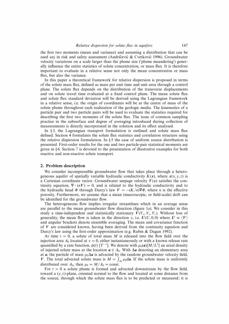
The heterogeneous flow implies irregular streamlines which in an average senseare parallel to the mean groundwater flow direction (figure 1a). We consider in thisstudy a time-independent and statistically stationary V (Vx, Vy, Vz). Without loss ofgenerality, the mean flow is taken in the direction x, i.e. U (U, 0, 0) where U ≡ 〈V 〉and angular brackets denote ensemble averaging. The mean and covariance functionof V are considered known, having been derived from the continuity equation andDarcy’s law using the first-order approximation (e.g. Rubin & Dagan 1992).

At time t = 0, a solute of total mass M is released into the flow field over theinjection area A0 located at x = 0, either instantaneously or with a known release ratequantified by a rate function, φ(t) [T−1]. We denote with ρ0(a)[M/L2] an areal densityof injected solute mass at the location a ∈ A0. With ∆a denoting an elementary areaat a, the particle of mass ρ0∆a is advected by the random groundwater velocity field,V . The total advected solute mass is M =

∫A0ρ0da. If the solute mass is uniformly

distributed over A0, then ρ0 = M/A0 = const.For t > 0 a solute plume is formed and advected downstream by the flow field,

toward a (y, z)-plane, oriented normal to the flow and located at some distance fromthe source, through which the solute mass flux is to be predicted or measured; it is

148 R. Andricevic and V. Cvetkovic

Meanflow

Accessibleenvironment

(a)

Samplingarea A

Plume

1

23

0

Sourcearea A0

Control plane

(b) Single realizationEnsemble mean

Mean travel time in a realization

Ensemble mean travel timeTime

Mas

s fl

ux

0

0

(c) Single realizationEnsemble mean

Ensemble mean travel timeTime

Mas

s fl

ux

0

0

Figure 1. Problem configuration and solute flux breakthrough ensemble averaging: (a) problemconfiguration, (b) absolute dispersion and (c) relative dispersion.

Relative dispersion for solute flux in aquifers 149

(a)Control plane

ú

è

A0

x

y

z

a

(b)Control plane

centre ofmass

ø

"

A0

x

y

z

aa0

centre ofmass

x

x

Figure 2. Definition sketch of particle displacement in (a) fixed frame of reference and(b) relative coordinates, for ρ0 = const.

referred to as the control plane (CP) (figures 1a and 2). Owing to velocity fluctuationson a scale equal to and smaller than the plume size, the plume is diffused anddistorted in an irregular manner (figure 1a). Velocity fluctuation on a scale largerthan the plume size cause the plume to ‘meander’ relative to the mean flow direction.

For a qualitative description of transport, consider first the breakthrough of thesolute plume across the entire control plane [MT−1]. Figures 1(b) and 1(c) schemat-ically show the difference between absolute and relative dispersion. The ensembleaverage for absolute dispersion accounts for both meandering and sub-plume velocityfluctuations; hence the dispersion is largest (figure 1b). Owing to relatively strong ge-ological heterogeneity, the temporal distribution of mass arrival (breakthrough) maydiffer significantly from realization to realization yielding the ensemble average fromthe fixed origin being quite different from any realization of the solute breakthrough(figure 1b). By comparison, the effect of meandering is removed from ensemble av-erages for relative dispersion, such that the spreading is generally smaller, and moreconsistent with the breakthrough in individual realizations (figure 1c). The expectedbreakthrough for relative dispersion is obtained from plume realizations where themean arrival times are set to coincide (figure 1c).

Next, consider the transverse position of the plume as it crosses the controlplane. Figure 2 shows displacement trajectories of particles advected from the source,described in absolute coordinates (figure 2a) and coordinates relative to the meantransverse displacement (figure 2b).

The main objective of the present study is to derive the statistical moments (meanand variance) of the solute flux in relative coordinates. In contrast to the absolutedispersion which concentrates on a single particle, relative dispersion relates to par-ticle pairs. Thus, we require the first two moments of travel time and transversedisplacement probability density functions (p.d.f.s) based on the statistics of motionof particle pairs. In order to evaluate the solute flux variance, the joint p.d.f. betweentwo particle pairs will be used. A particular problem to be addressed in the presentstudy is how to define and compute a global measure of plume statistical structure inspace and time, in analogy to the distance–neighbour function of Richardson (1926).

150 R. Andricevic and V. Cvetkovic

3. Lagrangian transport formulation3.1. Kinematical relationships

Traditional description of advective transport is by the trajectory X = X (t; a) whereX (0; a) = a is the point of injection at t = 0 (Taylor 1921). The statistics ofX (Xx,Xy, Xz) can be approximately related to the statistics of the groundwatervelocity field, V (x), as well as to the statistics of the hydraulic conductivity (e.g.Dagan 1984).

In our following analysis we quantify advective transport by the Lagrangian space–time process (τ, η), rather than the space process X (e.g. Dagan et al. 1992; Cvetkovic& Dagan 1994). τ(x; a) is a time process and quantifies the travel (arrival) time ofthe advective particle from the origin, a(0, ay, az), to a control plane (CP) at x. Weassume the solute parcel moves in the direction of the mean flow and τ is positiveand finite. η(η, ζ) is a space process that quantifies the transverse displacement, whereη(0; a) = a (figure 2).

The travel time τ can be obtained formally as τ(x; a) = X−1x (x; a), or explicitly as

τ(x; a) =

∫ x

0

dξ

Vx(ξ, η, ζ). (1)

The components of the transverse vector can be evaluated from Xy and Xz as

η(x; a) = Xy[τ(x; a); a], ζ(x; a) = Xz[τ(x; a); a], (2)

or from the velocity field explicitly as

η(x; a) =

∫ x

0

Vy(ξ, η, ζ)

Vx(ξ, η, ζ)dξ, ζ(x; a) =

∫ x

0

Vz(ξ, η, ζ)

Vx(ξ, η, ζ)dξ. (3)

Equations (1)–(3) provide the basic random variables for a single advecting soluteparticle.

The basic random variables that quantify the advection of the plume as a wholeare the areally averaged travel time and transverse displacement defined as

T (x;A0) ≡1

A0

∫A0

τ(x; a) da, (4)

Y (x;A0) ≡1

A0

∫A0

η(x; a) da, (5)

T (x;A0) and Y (x;A0)[Y (x;A0), Z(x;A0)] represent the mean travel time and meantransverse displacement for the entire plume crossing the CP. We emphasize thedependence of T and Y on the source size and the source shape, for notationalsimplicity denoted by A0. Both T (4) and Y (5) are defined as kinematical quantities;only in the case of ρ0(a) = const., do T and Y also represent the travel time andtransverse displacement of the centre of mass of the plume.

The basic random variables for describing the state of relative dispersion of a plumeof particles advected by a random velocity field, V (x), are

θ(x; a, A0) ≡ τ(x; a)− T (x;A0) =1

A0

∫A0

∆τ(x; a, a′)da′,

ϑ(x; a, A0) ≡ η(x; a)− Y (x;A0) =1

A0

∫A0

∆η(x; a, a′)da′,

(6)

with ϑ(ϑ, χ); θ and ϑ quantify fluctuations of the particle transport variables τ and η

Relative dispersion for solute flux in aquifers 151

from the plume transport variables T and Y . In (6),

∆τ(x; a, a′) ≡ τ(x; a)− τ(x; a′), ∆η(x; a, a′) ≡ η(x; a)− η(x; a′) (7)

represent a travel time difference and transverse separation at the CP for a particlepair.

3.2. Solute mass flux and discharge

General mass balance equations for solute undergoing mass transfer reactions are

∂C

∂t+ V · ∇C = ψm(C,N),

∂N

∂t= ψim(C,N), (8)

where we consider advection only, and where the fluid mass balance equation hasbeen used. In (8), C is the mobile and N the immobile solute concentration, withthe corresponding sink/source terms denoted as ψm and ψim. In the following werestrict our discussion to linear mass transfer reactions. Cvetkovic & Dagan (1994)showed how solute advection along random trajectories can be coupled with the linearreactions yielding the solution in terms of a time retention function γ(t, τ), which isavailable in analytical forms for a wide range of linear solute mass transfer processes.Note that for nonlinear reactions the retention function would depend on the initialand/or boundary concentration (e.g. Dagan & Cvetkovic 1996; Cvetkovic & Dagan1996).

In aquifers, the migrating solute is detected from a single or an array of drilledwells (boreholes). The corresponding sampling area is denoted by A and its valuewill depend on the sampling method used. Thus we seek to predict the statisticalproperties of the solute flux averaged over A. Integrating the solute flux for a singleparticle, ∆q ≡ ρ0(a) daΓ (t, τ) δ(y − η), over the injection area A0, averaging overthe sampling area A(y) centred at y(y, z) within the CP, yields the solute mass fluxcomponent orthogonal to the CP at x as

q(t, y; x, A) =1

A

∫A0

∫A

ρ0(a)Γ (t, τ)δ(y′ − η)dy′da, (9)

where

Γ (t, τ) ≡∫ t

0

φ(t− t′)γ(t′, τ)dt′ (10)

and φ(t)[T−1] is the injection rate. The time retention function γ(t, τ) is the solutionfor a solute pulse of the advection–reaction system (8), transformed onto an advectionflow path (Cvetkovic & Dagan 1994). For instantaneous release, φ ≡ δ(t); for non-reactive solute γ ≡ δ(t−τ). For instantaneous release of non-reactive solute (10) yieldsΓ = δ(t− τ). Note that the concentration C obtained from (8) and the solute flux fora single particle, ∆q, are related as ∆q = CVx(x, η, ζ).

The dependence of q on A emphasizes that the solute flux is averaged (or upscaled)over A and, hence, its statistics depend on the sampling area A. Note that in followingexpressions, dependence of the sampling area, A, on y is understood and will not bestated explicitly. From the solute mass flux we define the solute discharge over thesampling area A, Q [MT−1], as

Q(t, y; x, A) = q(t, y; x, A) A, (11)

where Q(t, y; x, A) quantifies the solute mass crossing A centred at y at time t. Statisticsof Q are readily obtained from statistics of q using (11).

152 R. Andricevic and V. Cvetkovic

4. Solute flux statisticsDuring any particular realization of a hypothetical experiment, the particle travel

time and transverse locations [τ(x; a), η(x; a)], will vary in a random manner due tothe fluctuations in V (x) on all scales. The plume travel time and transverse locations[T (x;A0),Y (x;A0)], will vary in an irregular manner resulting from the velocityfluctuations on the scale larger than the plume size; these variations would decreaseas the plume size increases. The random quantities [θ(x; a, A0), ϑ(x; a, A0)] vary in arandom manner due to velocity fluctuations on a scale smaller than the plume size.In this section we wish to compute the relative first two moments of solute flux usingthe statistics of [θ(x;A0, a), ϑ(x;A0, a)], and [T (x;A0),Y (x;A0)].

4.1. Probabilistic model of relative dispersion

The basic probability density functions (p.d.f.s) for describing the transport of a soluteplume are

f1(τ− T , η − Y , T ,Y ; x, A0, a)≡ f1(θ, ϑ, T ,Y ; x, A0, a),

f2(τ− T , τ′ − T , η − Y , η′ − Y , T ,Y ; x, A0, a, b)≡ f2(θ, θ′, ϑ, ϑ′, T ,Y ; x, A0, a, b).

}(12)

The p.d.f.s f1 and f2 are functions of the location of the CP, x, of the size and shapeof the source area, indicated by A0, and of the particle initial position a. The subscript1 in (12) indicates that the p.d.f. f1 is based on the statistics of one particle, whereasthe subscript 2 indicates that f2 moments are computed from two particles located ata and b. In (12), τ = τ(x; a), η = η(x; a) and τ′ = τ(x; b), η′ = η′(x; b).

Following the definitions of θ = τ− T and ϑ = η − Y , the basic p.d.f.s describingparticle transport in an absolute sense are obtained from (12) as

f1(τ, η; x, A0, a) =

∫ ∞0

∫ ∞0

f1(θ, ϑ, T ,Y ; x, A0, a) dT dY ,

f2(τ, τ′, η, η′; x, A0, a, b) =

∫ ∞0

∫ ∞0

f2(θ, θ′, ϑ, ϑ′, T ,Y ; x, A0, a, b) dT dY ,

(13)

Using the theorem on conditional probabilities, (13) can alternatively be written as

f1(τ, η; x, A0, a) =

∫ ∞0

∫ ∞0

f1(θ, ϑ | T ,Y ; x, A0, a)f(T ,Y ) dT dY ,

f2(τ, τ′, η, η′; x, A0, a, b) =

∫ ∞0

∫ ∞0

f2(θ, θ′, ϑ, ϑ′ | T ,Y ; x, A0, a, b) f(T ,Y ) dT dY ,

(14)

where f1(· | T ,Y ) and f2(· | T ,Y ) are conditional p.d.f.s, and f(T ,Y ) quantifies plumemeandering within the ensemble.

The advection of a plume as a whole is statistically described by the p.d.f.f(T ,Y ; x, A0), which provides information on the degree of uncertainty in the plumeposition and arrival at the CP. This p.d.f. may be useful for designing the totalmonitoring network size in the vicinity of potential source areas (e.g. landfills orwaste repositories). In addition, f(T ,Y ; x, A0) is the reducible uncertainty throughmeasurement conditioning. Collecting measurements at fixed locations or sequentiallyin stages can be used to condition f(T ,Y ; x, A0) and ultimately reduce the uncertaintyin predicting the migration of a plume as a whole.

Our main focus here is to study the effect of sub-plume velocity fluctuations on themean and variance of the reactive solute mass flux at the CP at x. By setting in (14)

f(T ,Y ) = δ(T − 〈τ〉) δ(Y − a0), (15)

Relative dispersion for solute flux in aquifers 153

where δ denotes the Dirac delta function, we eliminate plume meandering, i.e. weeliminate effects of V fluctuations on a scale larger than the plume size; a0(a0x =0, a0y , a0z ) is the centroid of A0.

Substituting (15) into (14), we obtain

fr1(τ, η; x, A0, a)≡∫ ∞

0

∫ ∞0

f1(θ, ϑ | T ,Y ; x, A0, a)δ(T − 〈τ〉) δ(Y − a0) dT dY

= f1(τ− 〈τ〉, η − a0 | 〈τ〉, a0; x, A0, a),

fr2(τ, τ′, η, η′; x, A0, a, b)≡

∫ ∞0

∫ ∞0

f2(θ, θ′, ϑ, ϑ′ | T ,Y ; x, A0, a, b)

×δ(T − 〈τ〉) δ(Y − a0) dT dY

= f2(τ− 〈τ〉, τ′ − 〈τ〉, η − a0, η′ − a0 | 〈τ〉, a0; x, A0, a, b),

(16)

where we denote with a superscript r the p.d.f.s that specifically quantify relativedispersion. The p.d.f.s fr1 and fr2 can in principle be constructed by performing a largenumber of plume realizations (forming an ensemble), superimposing mean arrivaltimes and displacements at the ensemble mean (〈τ〉, a0) and then evaluating one- andtwo-particle advective transport statistics (see figure 1c).

4.2. Mean and variance

Taking the expected value of q (9) with fr1 (16) we obtain

〈q(t, x)〉 =1

A

∫A0

∫A

∫ ∞0

ρ0(a)Γ (t, τ)fr1(τ, y′; x, a) dτ dy′ da. (17)

For simplicity, we omit hereafter explicit dependence on A0 and A which is to beunderstood. For a non-reactive solute pulse, with sampling over a point (i.e. A→ 0),we get

〈q(t, x)〉 =

∫A0

ρ0(a) fr1(t, y; x, a) da. (18)

The variance of the solute flux is evaluated as

σ2q(t, x) ≡

⟨q2⟩− 〈q〉2 , (19)

where ⟨q2(t, x)

⟩=

1

A2

∫A0

∫A0

ρ0(a)ρ0(b)F(t, y; x, a, b) da db (20)

and

F ≡∫A

∫A

∫ ∞0

∫ ∞0

Γ (t, τ)Γ (t, τ′)fr2(τ, τ′, y′, y′′; x, a, b) dτ dτ′ dy′ dy′′.

For a non-reactive solute pulse with sampling over a point (i.e. A→ 0), we have⟨q2(t, x)

⟩=

∫A0

∫A0

ρ0(a) ρ0(b) fr2(t, t, y, y; x, a, b) da db. (21)

The above expressions for 〈q〉 and σ2q for reactive and non-reactive solute are

analogous in form to the expressions in the absolute dispersion formulation, where fr1and fr2 are substituted by the corresponding p.d.f.s f1 and f2 (e.g. Dagan et al. 1992;Cvetkovic et al. 1992; Andricevic & Cvetkovic 1996).

154 R. Andricevic and V. Cvetkovic

4.3. Correlation structure

The correlation structure of the solute flux, or discharge, represents a statisticalfunction of potential interest in several applications, such as monitoring networkdesign, measurement conditioning, remediation design, etc. It describes the correlationbetween two solute particles at different locations in space–time coordinates observedat the CP. Since q and consequently Q are not stationary random functions, we writethe covariance between two points in space and time as

〈q(t1, y1; x)q(t2, y2; x)〉

where the dependence is on t1, y1 and t2, y2, i.e. on six variables.Generally it is not possible to use techniques developed for stationary random

functions to evaluate the above expression. However, we define the integral form ofthe above statistical function as

P (t∗, y∗; x) ≡∫ ∫

〈q(t, y; x)q(t+ t∗, y + y∗; x)〉 dt dy/∫ ∫

σ2q(t, y; x) dt dy, (22)

where integration is over all time and over the entire control plane at x. The aboveintegral correlation measure depends only on three variables in the three-dimensionalcase: the temporal lag t∗ and the two components of the transverse lag vector y∗.Furthermore, P (t∗, y∗; x) is quadrant symmetric (which implies statistical homogeneityin a weak sense, see e.g. Vanmarcke 1983) and is analogous to the distance–neighbourfunction of Richardson (1926). For the solute flux it behaves like a correlationfunction. A similar finding for the transverse spreading was reported by Chatwin &Sullivan (1979) in turbulent diffusion experiments at Lake Huron.

The solute flux correlation measure in (22) is a measure of solute flux structurethroughout the plume with all parts being given the same weight. For a given temporallag t∗ and spatial lag y∗, (22) represents the effective correlation measure at x for theentire plume. This correlation measure is based on the relative dispersion solution andprovides the actual measure of correlation between two points in a single realization.For example, the correlation scale in the transverse direction can be used as a guidelinefor transverse spacing between sampling wells at CP and the correlation scale in timecan be used as a guideline for sampling frequency of measurements.

4.4. One- and two-particle moments

In the following, we compute the first few moments of the basic p.d.f.s f1(θ, ϑ, T ,Y ; x, a)and f2(θ, θ

′, ϑ, ϑ′, T ,Y ; x, a, b).The first moments of f1 are computed as

〈θ(x; a)〉= 1

A0

∫A0

〈∆τ(x; a, a′)〉 da′ = 0,

〈ϑ(x; a)〉= 1

A0

∫A0

〈∆η(x; a, a′)〉 da′ = a− a0,

〈T (x)〉= 1

A0

∫A0

〈τ(x; a′)〉 da′ = 〈τ(x)〉,

〈Y (x)〉= 1

A0

∫A0

〈η(x; a′)〉 da′ = a0,

(23)

where a0(a0x = 0, a0y , a0z ) is the centroid of A0.

Relative dispersion for solute flux in aquifers 155

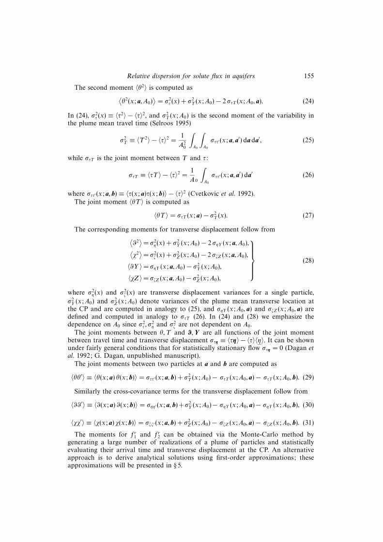
The second moment 〈θ2〉 is computed as⟨θ2(x; a, A0)

⟩= σ2

τ (x) + σ2T (x;A0)− 2 στT (x;A0, a). (24)

In (24), σ2τ (x) ≡ 〈τ2〉 − 〈τ〉2, and σ2

T (x;A0) is the second moment of the variability inthe plume mean travel time (Selroos 1995)

σ2T ≡ 〈T 2〉 − 〈τ〉2 =

1

A20

∫A0

∫A0

σττ′(x; a, a′) da da′, (25)

while στT is the joint moment between T and τ:

στT ≡ 〈τT 〉 − 〈τ〉2 =1

A 0

∫A0

σττ′(x; a, a′) da′ (26)

where σττ′(x; a, b) ≡ 〈τ(x; a)τ(x; b)〉 − 〈τ〉2 (Cvetkovic et al. 1992).The joint moment 〈θT 〉 is computed as

〈θT 〉 = στT (x; a)− σ2T (x). (27)

The corresponding moments for transverse displacement follow from⟨ϑ2⟩

= σ2η(x) + σ2

Y (x;A0)− 2 σηY (x; a, A0),⟨χ2⟩

= σ2ζ (x) + σ2

Z (x;A0)− 2 σζZ (x; a, A0),

〈ϑY 〉= σηY (x; a, A0)− σ2Y (x;A0),

〈χZ〉= σζZ (x; a, A0)− σ2Z (x;A0),

(28)

where σ2η(x) and σ2

ζ (x) are transverse displacement variances for a single particle,

σ2Y (x;A0) and σ2

Z (x;A0) denote variances of the plume mean transverse location atthe CP and are computed in analogy to (25), and σηY (x;A0, a) and σζZ (x;A0, a) aredefined and computed in analogy to στT (26). In (24) and (28) we emphasize thedependence on A0 since σ2

τ , σ2η and σ2

ζ are not dependent on A0.The joint moments between θ, T and ϑ,Y are all functions of the joint moment

between travel time and transverse displacement στη ≡ 〈τη〉 − 〈τ〉〈η〉. It can be shownunder fairly general conditions that for statistically stationary flow στη = 0 (Dagan etal. 1992; G. Dagan, unpublished manuscript).

The joint moments between two particles at a and b are computed as

〈θθ′〉 ≡ 〈θ(x; a) θ(x; b)〉 = σττ′(x; a, b) + σ2T (x;A0)− στT (x;A0, a)− στT (x;A0, b). (29)

Similarly the cross-covariance terms for the transverse displacement follow from

〈ϑϑ′〉 ≡ 〈ϑ(x; a) ϑ(x; b)〉 = σηη′(x; a, b)+σ2Y (x;A0)− σηY (x;A0, a)− σηY (x;A0, b), (30)

〈χχ′〉 ≡ 〈χ(x; a) χ(x; b)〉 = σζζ ′(x; a, b) + σ2Z (x;A0)− σζZ (x;A0, a)− σζZ (x;A0, b). (31)

The moments for fr1 and fr2 can be obtained via the Monte-Carlo method bygenerating a large number of realizations of a plume of particles and statisticallyevaluating their arrival time and transverse displacement at the CP. An alternativeapproach is to derive analytical solutions using first-order approximations; theseapproximations will be presented in § 5.

156 R. Andricevic and V. Cvetkovic

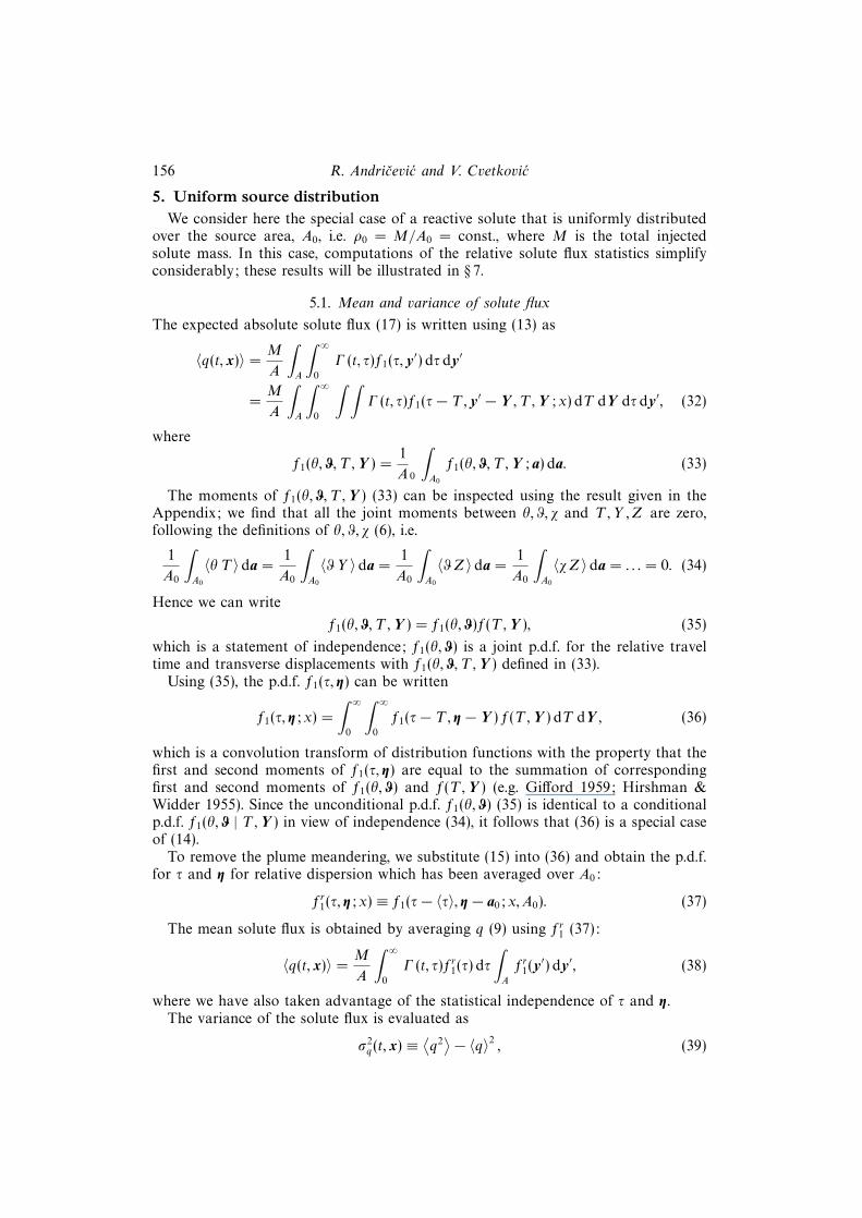
5. Uniform source distributionWe consider here the special case of a reactive solute that is uniformly distributed

over the source area, A0, i.e. ρ0 = M/A0 = const., where M is the total injectedsolute mass. In this case, computations of the relative solute flux statistics simplifyconsiderably; these results will be illustrated in § 7.

5.1. Mean and variance of solute flux

The expected absolute solute flux (17) is written using (13) as

〈q(t, x)〉 =M

A

∫A

∫ ∞0

Γ (t, τ)f1(τ, y′) dτ dy′

=M

A

∫A

∫ ∞0

∫ ∫Γ (t, τ)f1(τ− T , y′ − Y , T ,Y ; x) dT dY dτ dy′, (32)

where

f1(θ, ϑ, T ,Y ) =1

A 0

∫A0

f1(θ, ϑ, T ,Y ; a) da. (33)

The moments of f1(θ, ϑ, T ,Y ) (33) can be inspected using the result given in theAppendix; we find that all the joint moments between θ, ϑ, χ and T , Y , Z are zero,following the definitions of θ, ϑ, χ (6), i.e.

1

A0

∫A0

〈θ T 〉 da =1

A0

∫A0

〈ϑY 〉 da =1

A0

∫A0

〈ϑZ〉 da =1

A0

∫A0

〈χZ〉 da = . . . = 0. (34)

Hence we can write

f1(θ, ϑ, T ,Y ) = f1(θ, ϑ)f(T ,Y ), (35)

which is a statement of independence; f1(θ, ϑ) is a joint p.d.f. for the relative traveltime and transverse displacements with f1(θ, ϑ, T ,Y ) defined in (33).

Using (35), the p.d.f. f1(τ, η) can be written

f1(τ, η; x) =

∫ ∞0

∫ ∞0

f1(τ− T , η − Y ) f(T ,Y ) dT dY , (36)

which is a convolution transform of distribution functions with the property that thefirst and second moments of f1(τ, η) are equal to the summation of correspondingfirst and second moments of f1(θ, ϑ) and f(T ,Y ) (e.g. Gifford 1959; Hirshman &Widder 1955). Since the unconditional p.d.f. f1(θ, ϑ) (35) is identical to a conditionalp.d.f. f1(θ, ϑ | T ,Y ) in view of independence (34), it follows that (36) is a special caseof (14).

To remove the plume meandering, we substitute (15) into (36) and obtain the p.d.f.for τ and η for relative dispersion which has been averaged over A0:

fr1(τ, η; x) ≡ f1(τ− 〈τ〉, η − a0; x, A0). (37)

The mean solute flux is obtained by averaging q (9) using fr1 (37):

〈q(t, x)〉 =M

A

∫ ∞0

Γ (t, τ)fr1(τ) dτ

∫A

fr1(y′) dy′, (38)

where we have also taken advantage of the statistical independence of τ and η.The variance of the solute flux is evaluated as

σ2q(t, x) ≡

⟨q2⟩− 〈q〉2 , (39)

Relative dispersion for solute flux in aquifers 157

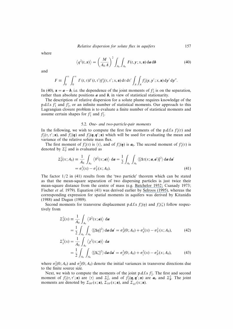
where ⟨q2(t, x)

⟩=

(M

A0 A

)2 ∫A0

∫A0

F(t, y; x, α) da db (40)

and

F ≡∫ ∞

0

∫ ∞0

Γ (t, τ)Γ (t, τ′)fr2(τ, τ′; x, α) dτ dτ′

∫A

∫A

fr2(y, y′; x, α) dy′ dy′′.

In (40), α = a− b, i.e. the dependence of the joint moments of fr2 is on the separation,rather than absolute positions a and b, in view of statistical stationarity.

The description of relative dispersion for a solute plume requires knowledge of thep.d.f.s fr1 and fr2, or an infinite number of statistical moments. Our approach to thisLagrangian closure problem is to evaluate a finite number of statistical moments andassume certain shapes for fr1 and fr2.

5.2. One- and two-particle-pair moments

In the following, we wish to compute the first few moments of the p.d.f.s fr1(τ) andfr2(τ, τ

′; α), and fr1(η) and fr2(η, η′; α) which will be used for evaluating the mean and

variance of the relative solute mass flux.The first moment of fr1(τ) is 〈τ〉, and of fr1(η) is a0. The second moment of fr1(τ) is

denoted by Σ2θ and is evaluated as

Σ2θ (x;A0) ≡

1

A0

∫A0

⟨θ2(x; a)

⟩da =

1

2

∫A0

∫A0

〈[∆τ(x; a, a′)]2〉 da da′

= σ2τ (x)− σ2

T (x;A0). (41)

The factor 1/2 in (41) results from the ‘two particle’ theorem which can be statedas that the mean-square separation of two dispersing particles is just twice theirmean-square distance from the centre of mass (e.g. Batchelor 1952; Csanady 1973;Fischer et al. 1979). Equation (41) was derived earlier by Selroos (1995), whereas thecorresponding expression for spatial moments in aquifers was derived by Kitanidis(1988) and Dagan (1989).

Second moments for transverse displacement p.d.f.s fr1(η) and fr1(ζ) follow respec-tively from

Σ2ϑ(x) ≡ 1

A0

∫A0

⟨ϑ2(x; a)

⟩da

=1

2

∫A0

∫A0

〈[∆η]2〉 da da′ = σ2ϑ(0;A0) + σ2

η(x)− σ2Y (x;A0), (42)

Σ2χ (x) =

1

A0

∫A0

⟨χ2(x; a)

⟩da

=1

2

∫A0

∫A0

〈[∆ζ]2〉 da da′ = σ2χ(0;A0) + σ2

ζ (x)− σ2Z (x;A0), (43)

where σ2ϑ(0;A0) and σ2

χ(0;A0) denote the initial variances in transverse directions dueto the finite source size.

Next, we wish to compute the moments of the joint p.d.f.s fr2. The first and secondmoment of fr2(τ, τ

′; α) are 〈τ〉 and Σ2θ , and of fr2(η, η

′; α) are a0 and Σ2ϑ . The joint

moments are denoted by Σθθ′(x; α), Σϑϑ′(x; α), and Σχχ′(x; α).

158 R. Andricevic and V. Cvetkovic

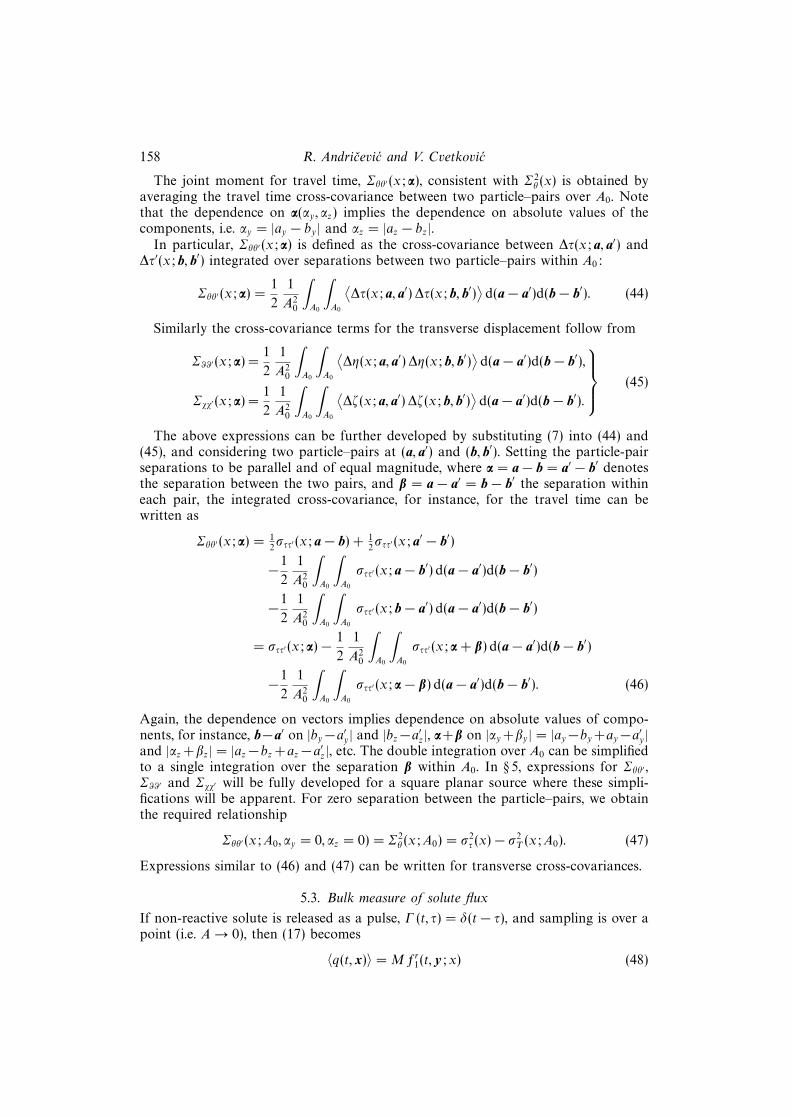
The joint moment for travel time, Σθθ′(x; α), consistent with Σ2θ (x) is obtained by

averaging the travel time cross-covariance between two particle–pairs over A0. Notethat the dependence on α(αy, αz) implies the dependence on absolute values of thecomponents, i.e. αy = |ay − by| and αz = |az − bz|.

In particular, Σθθ′(x; α) is defined as the cross-covariance between ∆τ(x; a, a′) and∆τ′(x; b, b′) integrated over separations between two particle–pairs within A0:

Σθθ′(x; α) =1

2

1

A20

∫A0

∫A0

⟨∆τ(x; a, a′) ∆τ(x; b, b′)

⟩d(a− a′)d(b− b′). (44)

Similarly the cross-covariance terms for the transverse displacement follow from

Σϑϑ′(x; α) =1

2

1

A20

∫A0

∫A0

⟨∆η(x; a, a′) ∆η(x; b, b′)

⟩d(a− a′)d(b− b′),

Σχχ′(x; α) =1

2

1

A20

∫A0

∫A0

⟨∆ζ(x; a, a′) ∆ζ(x; b, b′)

⟩d(a− a′)d(b− b′).

(45)

The above expressions can be further developed by substituting (7) into (44) and(45), and considering two particle–pairs at (a, a′) and (b, b′). Setting the particle-pairseparations to be parallel and of equal magnitude, where α = a− b = a′ − b′ denotesthe separation between the two pairs, and β = a − a′ = b − b′ the separation withineach pair, the integrated cross-covariance, for instance, for the travel time can bewritten as

Σθθ′(x; α) = 12σττ′(x; a− b) + 1

2σττ′(x; a′ − b′)

−1

2

1

A20

∫A0

∫A0

σττ′(x; a− b′) d(a− a′)d(b− b′)

−1

2

1

A20

∫A0

∫A0

σττ′(x; b− a′) d(a− a′)d(b− b′)

= σττ′(x; α)− 1

2

1

A20

∫A0

∫A0

σττ′(x; α+ β) d(a− a′)d(b− b′)

−1

2

1

A20

∫A0

∫A0

σττ′(x; α− β) d(a− a′)d(b− b′). (46)

Again, the dependence on vectors implies dependence on absolute values of compo-nents, for instance, b−a′ on |by−a′y| and |bz−a′z|, α+β on |αy+βy| = |ay−by+ay−a′y|and |αz +βz| = |az−bz +az−a′z|, etc. The double integration over A0 can be simplifiedto a single integration over the separation β within A0. In § 5, expressions for Σθθ′ ,Σϑϑ′ and Σχχ′ will be fully developed for a square planar source where these simpli-fications will be apparent. For zero separation between the particle–pairs, we obtainthe required relationship

Σθθ′(x;A0, αy = 0, αz = 0) = Σ2θ (x;A0) = σ2

τ (x)− σ2T (x;A0). (47)

Expressions similar to (46) and (47) can be written for transverse cross-covariances.

5.3. Bulk measure of solute flux

If non-reactive solute is released as a pulse, Γ (t, τ) = δ(t− τ), and sampling is over apoint (i.e. A→ 0), then (17) becomes

〈q(t, x)〉 = M fr1(t, y; x) (48)

Relative dispersion for solute flux in aquifers 159

i.e. the solute mass flux is proportional to fr1. The outstanding feature for soluteflux advective transport is the average temporal length of a plume (spreading ofbreakthrough) and transverse width of a plume. For non-reactive solute, a singlemeasure of this temporal length and transverse width is `θ(x;A0) and `ϑ(x;A0),respectively, where

`θ(x;A0)≡{

1

M

∫(t− 〈τ〉)2 〈q〉 dt

}1/2

=

{∫t2 fr1(t; x, A0) dt

}1/2

= Σθ,

`ϑ(x;A0)≡{

1

M

∫(y − a0)

2 〈q〉 dy}1/2

=

{∫y2 fr1(y; x, A0) dy

}1/2

= Σϑ

(49)

and `ϑ = [`η, `ζ]. As a consequence of mass conservation, the magnitude of the meannon-reactive solute flux is of the order (M/`θ`η`ζ) for the bulk of the plume at theCP.

6. First-order resultsThe hydraulic conductivity, K , is assumed to be a statistically stationary random

space function, log-normally distributed, i.e. K = Kg exp(k), where k : N(0, σ2k ), Kg is

the geometric mean, σ2k is the log-hydraulic conductivity variance, and k is spatially

correlated following a negative exponential function with the integral scale I . Theresulting velocity field in the aquifer, V (x), is also a statistically stationary randomspace function assumed to be steady with the mean hydraulic gradient parallel tothe x-coordinate axis. The injection plane set at the origin, x = 0, is assumed forsimplicity as a square, A0 = H ×H . In the following, we focus on computing Σ2

θ , Σ2ϑ ,

Σθθ′ and Σϑϑ′ which will be used for illustration of results.

6.1. Computation of Σ2θ and Σ2

ϑ

To evaluate the second moments required for relative p.d.f. fr1, we employ the first-order approximation in the velocity field which is based on the assumption that thestreamlines do not deviate significantly from the mean fluid direction (e.g. Dagan1984; Dagan et al. 1992). Expanding (1) and (3) we get at first-order

τ(x; a) =

∫ x

0

[1

U− ux(ξ, ay, az)

U2

]dξ, (50)

η(x; a) =

∫ x

0

uy(ξ, ay, az)

Udξ, (51)

ζ(x; a) =

∫ x

0

uz(ξ, ay, az)

Udξ, (52)

where ui(x, ay, az) is the velocity fluctuation in the i-direction, and the first-orderapproximation of the expansion (1 + ux/U)−1 is used, i.e. (1 + ux/U)−1 ≈ (1− ux/U).Thus, the travel time difference between two particles follows from

∆τ(x; a, a′) =1

U2

∫ x

0

ux(ξ, a′y, a′z) dξ − 1

U2

∫ x

0

ux(ξ, ay, az) dξ. (53)

The second moment for the relative travel time of a plume of particles, for a planar

160 R. Andricevic and V. Cvetkovic

source of size A0 = H ×H , follows from (24):

Σ2θ (x;H) =

1

2

1

A20

∫A0

∫A0

⟨[∆τ(x; a, a′)]2

⟩da da′ = σ2

τ (x)− σ2T (x;H)

=2

U2

∫ x

0

(x− ξ)Cux(ξ, 0, 0)dξ

− 8

H4U2

∫ H

0

∫ H

0

∫ x

0

(H − αy)(H − αz)(x− ξ)Cux(ξ, αy, αz)dξ dαy dαz, (54)

where αy ≡ |ay−a′y|, αz ≡ |az−a′z|, and Cux is the covariance function of the normalizedfluid velocity ux/U, available in a closed form (e.g. Rubin & Dagan 1992).

Similarly for transverse displacements, the separation between two particles followsfrom

∆η(x; a, a′) =

∫ x

0

uy(ξ, ay, az)

Udξ −

∫ x

0

uy(ξ, a′y, a′z)

Udξ, (55)

∆ζ(x; a, a′) =

∫ x

0

uz(ξ, ay, az)

Udξ −

∫ x

0

uz(ξ, a′y, a′z)

Udξ. (56)

The second moment follows from

Σ2ϑ(x;H) = σ2

ϑ(0;H) + 2

∫ x

0

(x− ξ)Cuy (ξ, 0, 0) dξ

− 8

H4

∫ H

0

∫ H

0

∫ x

0

(H − αy)(H − αz)(x− ξ)Cuy (ξ, αy, αz) dξ dαy dαz, (57)

Σ2χ (x;H) = σ2

χ(0;H) + 2

∫ x

0

(x− ξ)Cuz (ξ, 0, 0)dξ

− 8

H4

∫ H

0

∫ H

0

∫ x

0

(H − αy)(H − αz)(x− ξ)Cuz (ξ, αy, αz) dξ dαy dαz, (58)

where Cuy and Cuz denote the covariance functions of the normalized fluctuationsuy/U and uz/U, respectively.

Plume meandering (advection of the plume as a whole) is described by the secondterm on the right-hand side in (54) for travel time, and by the third term in (57)and (58) for transverse displacements. These terms constitute the second moment off(T ,Y ; x) and in conjunction with the ensemble mean can be used to hypothesizethe shape of f(T ,Y ; x).

6.2. Computation of Σθθ′ and Σϑϑ′

For the travel time joint p.d.f., fr2, we need to evaluate the cross-covariance termbetween two pairs of particles using the travel time differences ∆τ(x; a, a′) and∆τ′(x; b, b′). From (29) and (53) we have

Σθθ′ =1

2

1

A20

∫A0

∫A0

⟨∆τ(x; a, a′)∆τ(x; b, b′)

⟩d(a− a′) d(b− b′)

=1

2

1

A20

∫A0

∫A0

1

U4

∫ x

0

∫ x

0

{〈ux(ξ, ay, az)ux(ξ′, by, bz)〉

−〈ux(ξ, a′y, a′z)ux(ξ′, by, bz)〉 − 〈ux(ξ, ay, az)ux(ξ′, b′y, b′z)〉+〈ux(ξ, a

′

y, a′

z)ux(ξ′, b′y, b

′z)〉} dξ dξ′ d(a− a′) d(b− b′). (59)

Relative dispersion for solute flux in aquifers 161

Considering again a planar source of size A0 = H ×H , (59) reduces to

Σθθ′(x;H, α) =2

U2

∫ x

0

(x− ξ)Cux(ξ, αy, αz) dξ

− 4

U2H4

∫ H

0

∫ H

0

∫ x

0

(H − βy)(H − βz)(x− ξ)Cux(ξ, αy + βy, αz + βz) dξ dβy dβz

− 4

U2H4

∫ H

0

∫ H

0

∫ x

0

(H − βy)(H − βz)(x− ξ)Cux(ξ, αy − βy, αz − βz) dξ dβy dβz, (60)

where α(αy, αz) denotes the separation vector between two particle-pairs and β(βy, βz)denotes the separation vector between particles within each pair, respectively.

Similarly for transverse displacement, the cross-covariance terms required for eval-uating the transverse joint p.d.f. follow from

Σϑϑ′(x;H, α) = 2

∫ x

0

(x− ξ)Cuy (ξ, αy, αz) dξ

− 4

H4

∫ H

0

∫ H

0

∫ x

0

(H − βy)(H − βz)(x− ξ)Cuy (ξ, αy + βy, αz + βz) dξ dβy dβz

− 4

H4

∫ H

0

∫ H

0

∫ x

0

(H − βy)(H − βz)(x− ξ)Cuy (ξ, αy − βy, αz − βz) dξ dβy dβz (61)

Σχχ′(x;H, α) = 2

∫ x

0

(x− ξ)Cuz (ξ, αy, αz) dξ

− 4

H4

∫ H

0

∫ H

0

∫ x

0

(H − βy)(H − βz)(x− ξ)Cuz (ξ, αy + βy, αz + βz) dξ dβy dβz

− 4

H4

∫ H

0

∫ H

0

∫ x

0

(H − βy)(H − βz)(x− ξ)Cuz (ξ, αy − βy, αz − βz) dξ dβydβz. (62)

7. Illustration examplesFor illustration purposes we consider a two-dimensional aquifer with transport

of non-reactive and reactive solute. In all cases the source is a line of length H atx = 0 and a control plane (line) is set at x = L; both H and L are normalized withthe log-hydraulic conductivity integral scale, I . The mean solute flux and solute fluxstandard deviation are computed as functions of time and transverse displacement atthe control plane. The sampling line, denoted by B, is also normalized with I , andrepresents an averaging window at the control plane. We assume complete mixingwithin B as is usually the case in practice when sampling contaminants in aquifers.

Taking again advantage of 〈τη〉 = 0, we write the p.d.f.s fr1 and fr2 as

fr1(τ, η; x) = fr1(τ; x) fr1(η; x),

fr2(τ, τ′, η, η′; x, αy) = fr2(τ, τ

′; x, αy)fr2(η, η

′; x, αy).

The mean solute flux defined in (38) is proportional to fr1(τ; x, A0), assumed tofollow a log-normal shape with arithmetic moments fr1(τ; x) = LN[〈τ〉 = x/U, Σ2

θ ],and to fr1(η; x) = N[0, Σ2

ϑ] which is assumed to follow a Gaussian distribution. Theassumptions of a Gaussian distribution for η and log-normal for τ are consistent withresults from numerical simulations (e.g. Bellin, Saladin & Rinaldo 1992; Cvetkovic,Cheng & Wen 1996). A Gaussian distribution for transverse particle displacement

162 R. Andricevic and V. Cvetkovic

is also consistent with observations in atmospheric turbulent diffusion (e.g. Csanady1973; Chatwin & Sullivan 1990). For computing the solute flux variance we hy-pothesize a joint log-normal p.d.f. for fr2(τ, τ

′; x,H, αy) and joint Gaussian p.d.f. forfr2(η, η

′; x,H, αy), evaluated with two-dimensional forms of (60) and (61). The abovechoice of distributions is only for illustrative purposes; other distributions, that areconsistant with numerical simulations or field experiments, could be used as alterna-tives.

7.1. Non-reactive case

For non-reactive solute injected over a line source of extent H , with ρ0 =const.[M/L−1], and a sampling window of length B centred at y, the mean solute fluxreduces from (38) to

〈q(t, x, y)〉 =M

Bfr1(t; x,H)

∫B

fr1(y′; x,H) dy′. (63)

The solute flux variance is σ2q(t, x, y) =

⟨q2⟩− 〈q〉2 where (40) reduces to⟨

q2(t, x, y)⟩

=M2

H2 B2

∫H

∫H

∫B

∫B

fr2(t, t; x,H, αy) fr2(y′, y′′; x,H, αy) dy′ dy′′ day da′y

(64)where αy = |ay − a′y| is a separation between two particle pairs, and M = ρ0 H .

We first analyse relative dispersion for the solute discharge across the entire CP, Q,obtained from (11) for A → ∞ (or B → ∞); thus only the marginal p.d.f. fr1(t; x,H)is required.

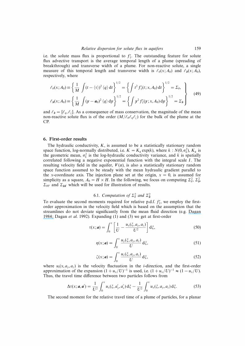
Figure 3 shows the first two moments of the solute discharge with σ2k = 0.5 and the

CP set at 20I from the source. Figures 3(a) and 3(b) describe the difference betweenthe absolute and relative dispersion for the mean solute discharge and the solutedischarge standard deviation, respectively. The two descriptions of the dispersionprocess converge for a larger source size with a faster convergence for the first (e.g.H > 10) than second moment (e.g. H > 20) of solute discharge. This indicates thatthe ergodicity in the mean is reached more rapidly than ergodicity in the secondmoment of solute discharge. In the limit H → ∞ equations (54) and (60) reduce totheir absolute dispersion results (Cvetkovic et al. 1992). In the limit H → 0, (54) and(60) approach zero, indicating that the relative dispersion does not exist for a pointsource and transport is described as meandering only.

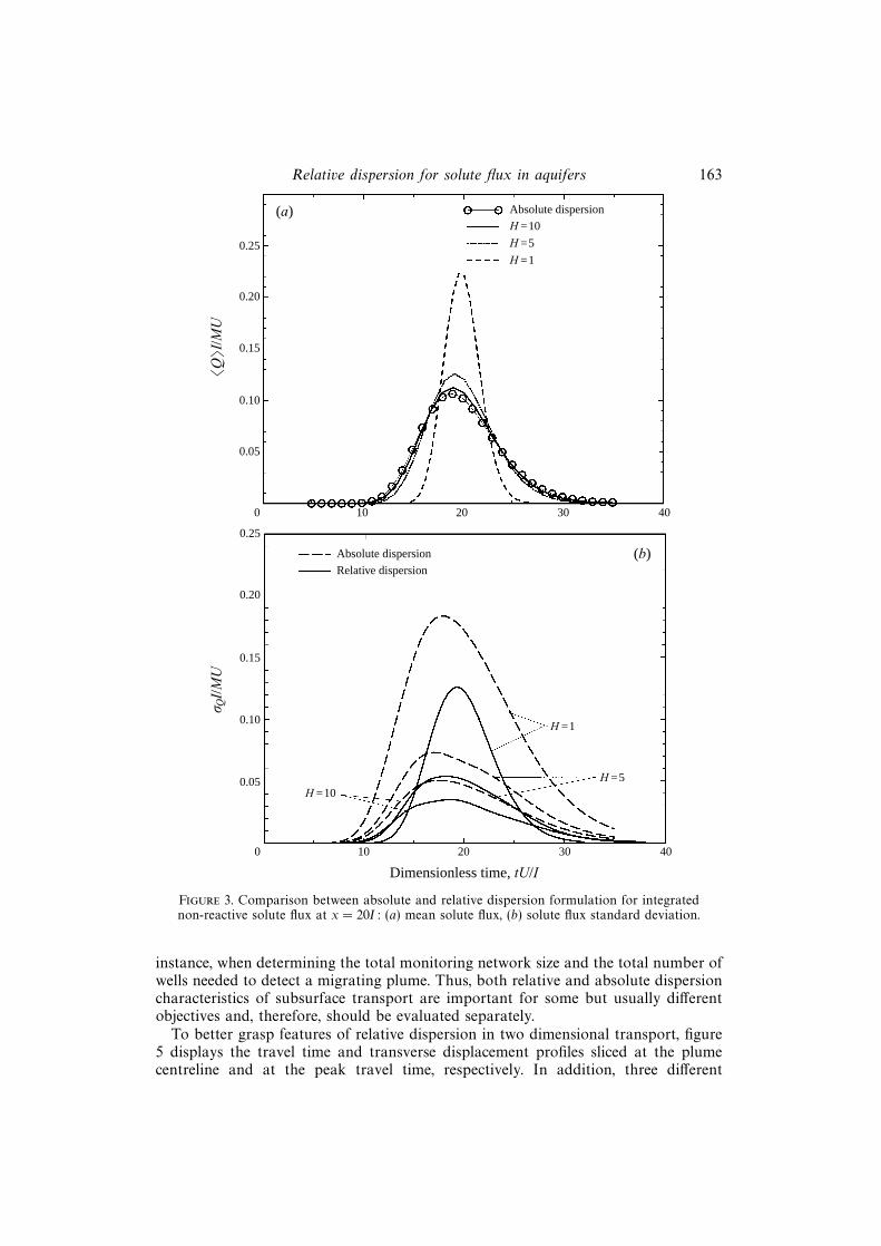
Figure 4 shows the mean and standard deviation of the solute flux as a functionof travel time and transverse displacement at the CP placed at 20I . The plume meanlocation at the CP is positioned on the ensemble mean travel time 〈τ〉 and transversedisplacement a0 = 0 to represent the relative spreading due to the velocity fluctuationson the scale smaller than the plume size. The velocity fluctuations on the scale largerthan plume size contribute to the plume meandering and they are removed fromthe relative solute flux formulation. The relative plume spreading displayed on figure4 provides important information for a certain class of environmental applications,in particular for the risk assessment where actual concentration fluctuations causepotential harm to humans, etc. Including the plume meandering in the overall en-semble would flatten the contaminant breakthrough, reduce the peak (figure 1b), andconsequently would underestimate the potential risk.

The uncertainty in the description of a plume centroid location is a consequence ofour inability to precisely estimate where the plume as a whole will migrate due to thelarger heterogeneity scale present in aquifers; it is of interest for some applications, for

Relative dispersion for solute flux in aquifers 163

0.25

0.20

0.15

0.10

0.05

0 10 20 30 40

Absolute dispersion

H =10

H =5

H =1

(a)©

Qª

I/M

U

H =1

H =5

0.25

0.20

0.15

0.10

0.05

0 10 20 30 40

Absolute dispersion

Relative dispersion

H =10

(b)

Dimensionless time, tU/I

ó QI/

MU

Figure 3. Comparison between absolute and relative dispersion formulation for integratednon-reactive solute flux at x = 20I: (a) mean solute flux, (b) solute flux standard deviation.

instance, when determining the total monitoring network size and the total number ofwells needed to detect a migrating plume. Thus, both relative and absolute dispersioncharacteristics of subsurface transport are important for some but usually differentobjectives and, therefore, should be evaluated separately.

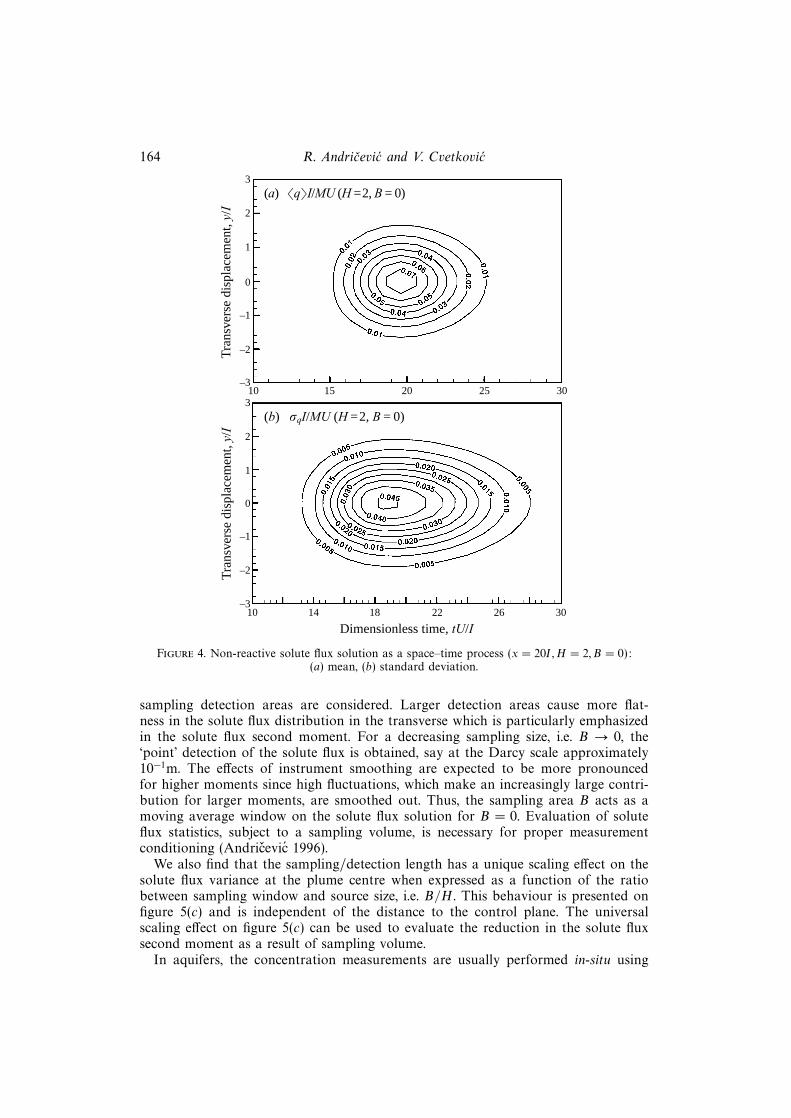
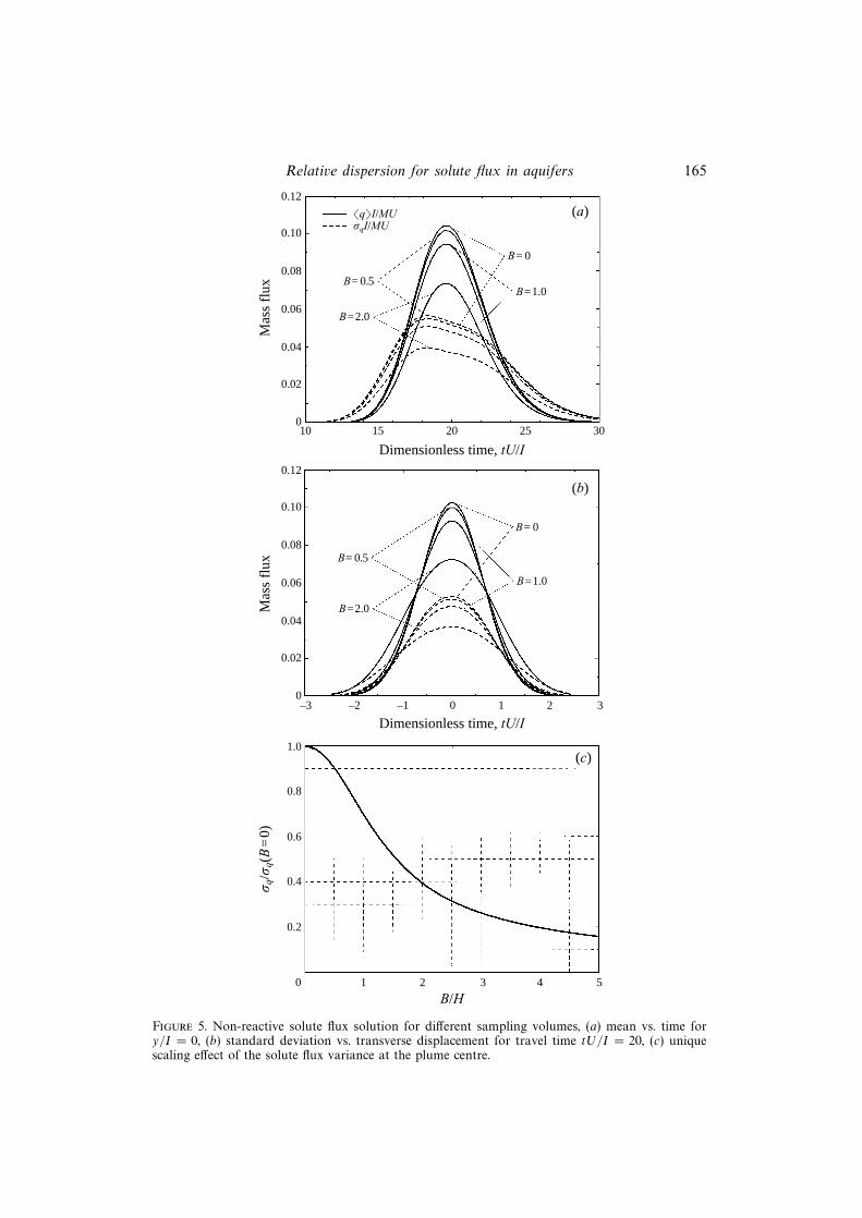
To better grasp features of relative dispersion in two dimensional transport, figure5 displays the travel time and transverse displacement profiles sliced at the plumecentreline and at the peak travel time, respectively. In addition, three different

164 R. Andricevic and V. Cvetkovic

Dimensionless time, tU/I

3

2

1

0

–1

–2

–310 15 20 25 30

(a) ©qªI/MU (H =2, B = 0)

Tra

nsve

rse

disp

lace

men

t, y/

I

3

2

1

0

–1

–2

–3

Tra

nsve

rse

disp

lace

men

t, y/

I

10 14 18 22 26 30

(b) óqI/MU (H =2, B = 0)

Figure 4. Non-reactive solute flux solution as a space–time process (x = 20I, H = 2, B = 0):(a) mean, (b) standard deviation.

sampling detection areas are considered. Larger detection areas cause more flat-ness in the solute flux distribution in the transverse which is particularly emphasizedin the solute flux second moment. For a decreasing sampling size, i.e. B → 0, the‘point’ detection of the solute flux is obtained, say at the Darcy scale approximately10−1m. The effects of instrument smoothing are expected to be more pronouncedfor higher moments since high fluctuations, which make an increasingly large contri-bution for larger moments, are smoothed out. Thus, the sampling area B acts as amoving average window on the solute flux solution for B = 0. Evaluation of soluteflux statistics, subject to a sampling volume, is necessary for proper measurementconditioning (Andricevic 1996).

We also find that the sampling/detection length has a unique scaling effect on thesolute flux variance at the plume centre when expressed as a function of the ratiobetween sampling window and source size, i.e. B/H . This behaviour is presented onfigure 5(c) and is independent of the distance to the control plane. The universalscaling effect on figure 5(c) can be used to evaluate the reduction in the solute fluxsecond moment as a result of sampling volume.

In aquifers, the concentration measurements are usually performed in-situ using

Relative dispersion for solute flux in aquifers 165

Dimensionless time, tU/I

©qªI/MUóqI/MU

0.12

0.10

0.08

0.06

0.04

0.02

010 15 20 25 30

(a)

B= 0

B=1.0B= 0.5

B=2.0

0.12

0.10

0.08

0.06

0.04

0.02

0

(b)

B= 0

B=1.0

B= 0.5

B=2.0Mas

s fl

uxM

ass

flux

Dimensionless time, tU/I–3 –2 –1 0 1 2 3

(c)

0 1 2 3 4 5

B/H

1.0

0.8

0.6

0.4

0.2

ó q/ó

q(B

=0)

Figure 5. Non-reactive solute flux solution for different sampling volumes, (a) mean vs. time fory/I = 0, (b) standard deviation vs. transverse displacement for travel time tU/I = 20, (c) uniquescaling effect of the solute flux variance at the plume centre.

166 R. Andricevic and V. Cvetkovic

well probes or by withdrawal of water by pumping. In either case, and particularlyin the latter, the volume of sampled aquifer is much larger than the pore scale and,therefore, complete mixing within the detection volume due to the sampling willoccur. This sampling practice in aquifers acts as instrument smoothing and does notallow detection of possible high solute fluctuations concentrated in the flow paths ona scale smaller than B. The effect of instrument smoothing is to drastically reducethe magnitude of solute flux higher-order moments. If additional temporal samplingtime is introduced (e.g. Destouni & Graham 1997), further smoothing would occur.

Although pore-scale dispersion will reduce the concentration fluctuations afteradvective transport has developed (i.e. the plume is stretched and distorted creatingmore surface area where pore-scale dispersion can occur), the quantification andverification of its impact on concentration fluctuations from measurements in aquifersis very difficult. Thus, the influence of pore-scale dispersion, if included in modelling,usually cannot be supported by measurement in the subsurface; it thus remainsdifficult to assess what is the actual pore-scale dispersion effect on the solute transport.However, a finite sampling area A and the pore-scale dispersion yield similar effectson concentration fluctuations, namely they both introduce concentration smoothingand reduce higher-order moments.

7.2. Effect of non-equilibrium sorption

For cases where solute is subject to equilibrium or non-equilibrium mass transferreactions between the fluid phase and surrounding material, the form of the timeretention function needs to be specified. If the migrating solute undergoes a sorption-desorption reaction controlled by first-order kinetics with

ψm = −α (Kd C −N)− k0 C, ψim = α (Kd C −N)− k0 N (65)

the time retention function is (e.g. Cvetkovic & Dagan 1994)

γ(t, τ) = exp[−(αKd + k0)t]δ(t− τ) + α2 Kdτ exp(−αKd τ− αt+ ατ− k0t)

×I1[α2 Kd τ(t− τ)]H(t− τ) (66)

where I1(z) ≡ I1(2z1/2)/z1/2 with I1 being the modified Bessel function of the first

kind of order one, α is the mass transfer rate, Kd is the distribution coefficientonce equilibrium is reached for reversible mass transfer, H(t − τ) is the Heavisidestep function, and k0 accounts for irreversible mass transfer (degradation in bothmobile and immobile phases, or decay). For α→∞, reversible mass transfer is underequilibrium conditions, and (66) reduces to γ = e−k0 t δ [t− (1 +Kd) τ].

Using (38) and (40), the first two moments of the solute flux are obtained as

〈q(t, x, y)〉 =M

B

∫B

∫ ∞0

γ(t, τ)fr1(τ; x) fr1(y′; x) dτ dy′ (67)

and σ2q(t, x, y) =

⟨q2⟩− 〈q〉2, where⟨

q2(t, x, y)⟩

=M2

H2B2

∫H

∫H

∫B

∫B

∫ ∞0

∫ ∞0

γ(t, τ)γ(t, τ′)

×fr2(τ, τ′; x,H, αy) fr2(y′, y′′; x,H, αy) dτ dτ′ dy′ dy′′ day da′y (68)

with αy = |ay − a′y|.Figure 6 shows the solute plume undergoing mass transfer processes with α∗ ≡

αI/U = 0.1 and Kd = 1, displayed in the two-dimensional transport coordinates,

Relative dispersion for solute flux in aquifers 167

Dimensionless time, tU/I

2

1

0

–1

–2

10 20 30 40 50

(a) ©qªI/MU (H =2, B = 0)

Tra

nsve

rse

disp

lace

men

t, y/

I

3

2

1

0

–1

–2

–3

Tra

nsve

rse

disp

lace

men

t, y/

I

10 20 30 40 50 60

(b) óqI/MU (H =2, B = 0)

60 70 80

70 80

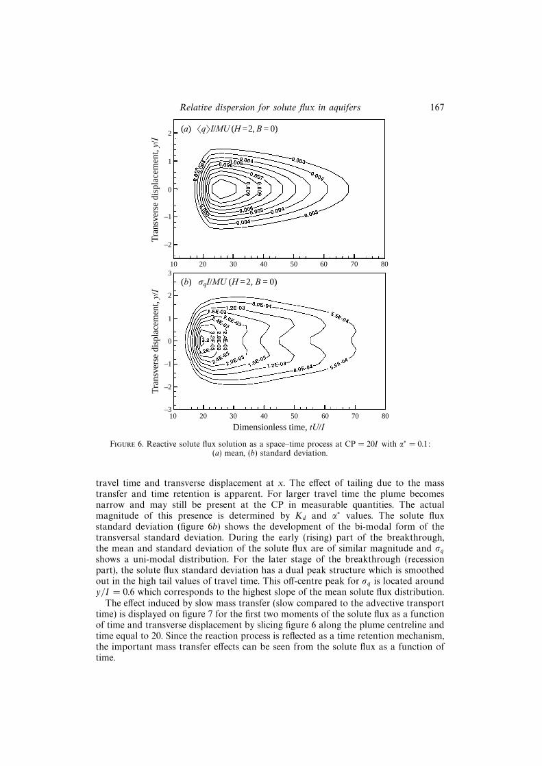
Figure 6. Reactive solute flux solution as a space–time process at CP = 20I with α∗ = 0.1:(a) mean, (b) standard deviation.

travel time and transverse displacement at x. The effect of tailing due to the masstransfer and time retention is apparent. For larger travel time the plume becomesnarrow and may still be present at the CP in measurable quantities. The actualmagnitude of this presence is determined by Kd and α∗ values. The solute fluxstandard deviation (figure 6b) shows the development of the bi-modal form of thetransversal standard deviation. During the early (rising) part of the breakthrough,the mean and standard deviation of the solute flux are of similar magnitude and σqshows a uni-modal distribution. For the later stage of the breakthrough (recessionpart), the solute flux standard deviation has a dual peak structure which is smoothedout in the high tail values of travel time. This off-centre peak for σq is located aroundy/I = 0.6 which corresponds to the highest slope of the mean solute flux distribution.

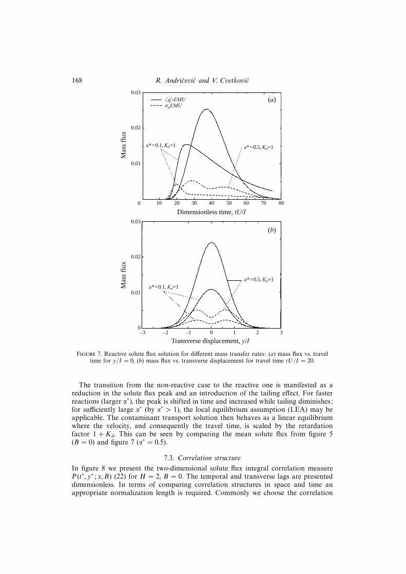
The effect induced by slow mass transfer (slow compared to the advective transporttime) is displayed on figure 7 for the first two moments of the solute flux as a functionof time and transverse displacement by slicing figure 6 along the plume centreline andtime equal to 20. Since the reaction process is reflected as a time retention mechanism,the important mass transfer effects can be seen from the solute flux as a function oftime.

168 R. Andricevic and V. Cvetkovic

Dimensionless time, tU/I

©qªI/MUóqI/MU

0.03

0.02

0.01

0 10 3020 40 50

(a)

0.03

0.02

0.01

0

(b)

Mas

s fl

uxM

ass

flux

Transverse displacement, y/I–3 –2 –1 0 1 2 3

60 70 80

α*=0.5, Kd=1α*=0.1, Kd=1

α*=0.5, Kd=1

α*=0.1, Kd=1

Figure 7. Reactive solute flux solution for different mass transfer rates: (a) mass flux vs. traveltime for y/I = 0, (b) mass flux vs. transverse displacement for travel time tU/I = 20.

The transition from the non-reactive case to the reactive one is manifested as areduction in the solute flux peak and an introduction of the tailing effect. For fasterreactions (larger α∗), the peak is shifted in time and increased while tailing diminishes;for sufficiently large α∗ (by α∗ > 1), the local equilibrium assumption (LEA) may beapplicable. The contaminant transport solution then behaves as a linear equilibriumwhere the velocity, and consequently the travel time, is scaled by the retardationfactor 1 + Kd. This can be seen by comparing the mean solute flux from figure 5(B = 0) and figure 7 (α∗ = 0.5).

7.3. Correlation structure

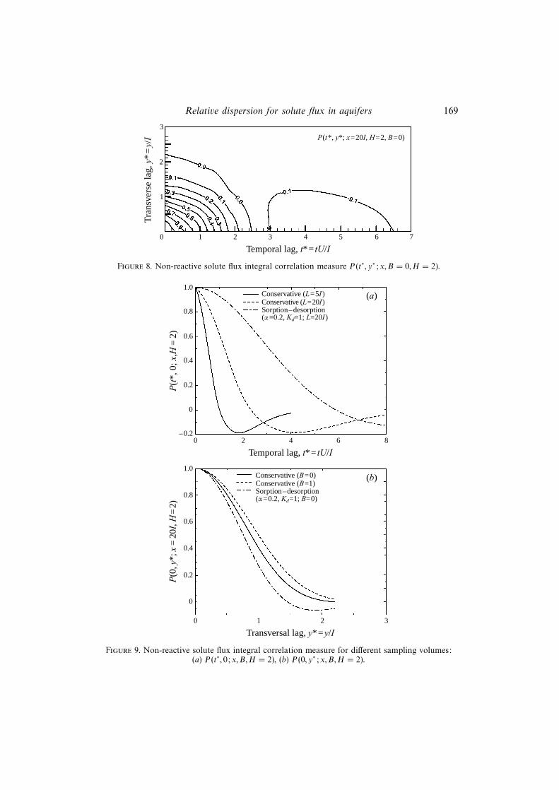
In figure 8 we present the two-dimensional solute flux integral correlation measureP (t∗, y∗; x, B) (22) for H = 2, B = 0. The temporal and transverse lags are presenteddimensionless. In terms of comparing correlation structures in space and time anappropriate normalization length is required. Commonly we choose the correlation

Relative dispersion for solute flux in aquifers 169

3

2

1

0 1 2 3 4 5 6 7

Temporal lag, t*= tU/I

Tra

nsve

rse

lag,

y*

=y/

I P(t*, y*; x=20I, H=2, B=0)

Figure 8. Non-reactive solute flux integral correlation measure P (t∗, y∗; x, B = 0, H = 2).

0

–0.20 2 4 6 8

Temporal lag, t*= tU/I

P(t

*, 0

; x,H

=2)

0.2

0.4

0.6

0.8

1.0Conservative (L=5I )Conservative (L=20I)Sorption–desorption(α=0.2, Kd=1; L=20I )

Conservative (B=0)Conservative (B=1)Sorption–desorption(α=0.2, Kd=1; B=0)

0 1 2 3

Transversal lag, y*=y/I

0

P(0

, y*;

x=

20I,

H=

2)

0.2

0.4

0.6

0.8

1.0

(a)

(b)

Figure 9. Non-reactive solute flux integral correlation measure for different sampling volumes:(a) P (t∗, 0; x, B,H = 2), (b) P (0, y∗; x, B,H = 2).

170 R. Andricevic and V. Cvetkovic

scale defined as the distance for the e−1 decrease of the correlation. Only in the caseof a negative exponential type of correlation function is the correlation scale thesame as the integral scale, the latter defined as the integral of the correlation functionnormalized with the variance. Figure 8 shows the correlation scale in the transversecoordinate to be around I and 1.5I for travel time. In words, two solute particles in asingle realization crossing the CP at the same time (t∗ = 0) are correlated within thedistance of I and similarly two solute particles crossing the CP at the same location(y∗ = 0) will be correlated in time within 1.5I . These two correlation measures mayprovide useful guidelines for designing sampling networks in the subsurface. Anyother correlation depending on both temporal and transverse lags can be deducedfrom figure 8.

Figure 9 shows a different sensitivity analysis of correlation measures of the soluteflux by keeping one coordinate lag equal to zero, i.e. the correlation measure alongthe plume centreline (figure 9a displays P (t∗, 0; x, B)) and transverse cross-section att = 〈τ〉 (figure 9b displays P (0, y∗; x, B)). Figure 9(a) depicts the development of thetemporal correlation scale for the CP located at 5I and 20I with a clear increaseof the correlation scale at the larger distance from the source. If, in addition, thesolute undergoes a sorption–desorption reaction, the temporal correlation is furtherincreased. That transverse correlation scale of the plume, P (0, y∗; x, B), on figure 9(b)shows an increase in the transverse correlation by considering the sampling detection(B = 1); however, when sorption–desorption is active, the transverse correlationscale is reduced compared to ‘point’ detection. The tailing effect (figure 6) causesa narrow plume which is the reason why the transverse correlation scale on figure9(b) is reduced. In all cases there is a smooth Gaussian-type correlation structurefor the transverse direction while the temporal correlation has a region of negativecorrelation and behaves like a hole-Gaussian-type correlation function.

8. SummaryRelative dispersion of the mass flux for non-reactive and reactive solute is presented

in terms of the first two moments, i.e. mean solute flux and solute flux variance. Themean solute flux is described as a space–time process where time refers to the soluteflux breakthrough and space refers to the transverse displacement distribution at thecontrol plane placed perpendicular to the mean flow direction. The statistical momentsfor describing the mean solute flux distribution are derived using the statistics of asingle particle pair while moments for the distribution of the solute flux variance arebased on the motion of two particle pairs. Statistics of the solute flux, as a space–timeprocess, fully describe the evolution of a contaminant plume in heterogeneous aquifers.

The results indicate that the relative dispersion of the solute flux approaches theabsolute dispersion when source size is increased. This convergence is faster in themean than in the standard deviation of the solute flux. For a decreasing source size,the difference between the absolute and relative dispersion formulations increases.The smoothing effect due to a finite sampling area influences the first two moments ofthe solute flux. This influence is more pronounced in the solute flux second-momentdistribution by reducing the peak with enhanced spreading in space and time. Thesolute flux solution for contaminants undergoing a sorption reaction shows the effectof tailing in arrival time with a bi-modal transverse distribution of the solute fluxsecond moment in the recession stage of the breakthrough.

The integrated correlation structure of the solute flux in (22) has been derived asan effective, global space–time measure of the migrating plume. When evaluated for a

Relative dispersion for solute flux in aquifers 171

fixed time, this correlation describes the probability that two points at the CP are inthe marked fluid and as such is a potentially useful indicator for optimizing spacingof sampling locations in aquifers. Conversely, when evaluated for a fixed point at theCP, P describes the temporal correlation of the breakthrough and can be used toassign the frequency of measurements.

The derived integral-form solution for the solute flux moments neglects the effect ofpore-scale dispersion. Pore-scale dispersion is due to velocity fluctuations on the scaleof the order of say 10−3 m, whereas the solute flux solution is based on the flow fieldevaluated from hydraulic data assumed to have been sampled on (or downscaled to)the Darcy scale, of the order of say 10−1 m. The pore-scale dispersion effect is knownto increase with transport time and affects most the solute flux higher moments. Itsmaximum impact is anticipated for point measurements (i.e. for A→ 0) which is ap-proximately on the Darcy scale (e.g. Graham & McLaughlin 1989; Li & McLaughlin1991; Kapoor & Gelhar 1994; Zhang & Neuman 1996; Dagan & Fiori 1997). In manyapplications, however, samples are taken over finite scales larger than the Darcy scale(i.e. finite A) such that the actual pore-scale effect is suppressed and difficult to detectdue to the mixing in the sampling volume. In addition, if sampling is over finite timeintervals it can only enhance the mixing in sampling (e.g. Destouni & Graham 1997).

The first-order approximation for the velocity field, distributional assumptions forτ and η, and an assumption for relating Lagrangian and Eulerian statistics, have beenemployed in this analysis for illustrative purposes. Extensive numerical simulations(e.g. Bellin et al. 1992; Chin & Wang 1992; Cvetkovic et al. 1996) as well as comparisonwith field data (Burr, Sudicky & Naff 1994) support distributional assumptions andindicate that the first-order approximation is robust for σ2

k at least up to 1. In realapplications and for higher σ2

k , numerical simulations can be used for determiningdistributions for τ and η as well as for computing their relevant statistics.

Knowledge of first two moments of the solute flux (or discharge) is often of directpractical interest, for instance, in risk management, remedial decisions, etc. How-ever, the sampling practice in aquifers is most frequently in terms of flux-averagedconcentration that is defined as Cf = q/Vn [ML−3] and hence directly related tothe solute flux. The groundwater flux at a point of measurement is proportionalto Vn and thereby also a random process; its statistics need to be combined withsolute flux statistics to yield the flux-averaged concentration statistics. For example,〈Cf〉 = (1/n)

∫(q/V )f(q, V ) dq dV defines the mean flux-averaged concentration (as-

suming constant effective porosity) where f(q, V ) denotes the joint p.d.f. between thesolute flux and groundwater velocity for a specific sampling scale. Thus, the solute fluxstatistics provide a basis for evaluating the statistics of the flux-averaged concentra-tion. The ability of the proposed framework to account for a finite sampling scale (i.e.A > 0) is crucial for conversion of the solute flux into the flux-averaged concentrationdata.

The authors wish to thank two anonymous reviewers, as well as Sten Berglund atthe Royal Institute of Technology in Stockholm, and Aldo Fiori at Terza Universita’di Roma, for their helpful comments and suggestions in the final preparation of themanuscript.

AppendixLet f(X,Y ; a) denote a joint p.d.f. of X and Y , which is dependent on a parameter

a. Let f(p, q; a) denote the moment generating function of f that has been obtained as

172 R. Andricevic and V. Cvetkovic

an appropriate transform of f where p and q are transform variables. The momentsof f are computed as

µmn ≡∫ ∫

Xm Y n f(X,Y ; a) dX dY = (−1)m+n ∂m+nf(p, q; a)

∂pm ∂qn(A 1)

for p = q = 0.Let F(X,Y ) be defined as

F(X,Y ) ≡ [f] =1

A

∫A

f(X,Y ; a) da, (A 2)

where a ∈ A; thus F is also a p.d.f. We wish to compute the moments of F asfunctions of the moments of f.

Applying the linear integral operator [ ] on both sides of (A 1) yields

[µmn] ≡∫ ∫

Xm Y n F(X,Y ) dX dY = (−1)m+n ∂m+nF(p, q)

∂pm ∂qn(A 3)

since F = [f]. Thus, the moments of F ≡ [f] are equal to the moments of f on which[ ] is applied. If the averaged joint moments are zero, we have F(X,Y ) = F(X)F(Y ).The above can be generalized to three or more random variables.

REFERENCES

Andricevic, R. 1996 Evaluation of sampling in the subsurface. Water Resour. Res. 32, 863–874.

Andricevic, R. & Cvetkovic, V. 1996 Evaluation of risk from contaminants migrating by ground-water. Water Resour. Res. 32, 611–621.

Batchelor, G. K. 1952 Diffusion in the field of homogeneous turbulence. II. The relative motionof particles. Proc. Camb. Phil. Soc. 48, 345–362.

Bellin, A., Saladin, P. & Rinaldo, A. 1992 Simulation of dispersion in heterogeneous porousformations: Statistics, first-order theories, convergence of computations. Water Resour. Res.28, 2211–2227.

Borgas, M. S. & Sawford, B. L. 1994 A family of stochastic models for two-particle dispersion inisotropic homogeneous stationary turbulence. J. Fluid Mech. 276, 69–99.

Burr, D. T., Sudicky, E. A. & Naff, R. L. 1994 Nonreactive and reactive solute transport in three-dimensional porous media: Mean displacement, plume spreading, and uncertainty. WaterResour. Res. 30, 791–817.

Chatwin, P. C. & Sullivan, P. J. 1979 The relative diffusion of a cloud of passive contaminant inincompressible turbulent flow. J. Fluid Mech. 91, 337–355.

Chatwin, P. C. & Sullivan, P. J. 1990 A simple and unifying physical interpretation of scalarfluctuation measurements from many turbulent shear flows. J. Fluid Mech. 212, 533–566.

Chin, D. A. & Wang, T. 1992 An investigation of the validity of first-order stochastic dispersiontheories in isotropic porous media. Water Resour. Res. 28, 1531–1542.

Cushman, J. H. & Ginn, T. R. 1993 Nonlocal dispersion in media with continuously evolving scalesof heterogeneity. Trans. Porous Media 13, 123–138.

Cvetkovic, V., Dagan, G. & Shapiro, A. 1992 A solute flux approach to transport in heterogeneousformations, 2, Uncertainty analysis. Water Resour. Res. 28, 1377–1388.

Cvetkovic, V. & Dagan, G. 1994 Transport of kinetically sorbing solute by steady random velocityin heterogeneous porous formations. J. Fluid Mech. 265, 189–215.

Cvetkovic, V., Cheng, H. & Wen, X.-H. 1996 Analysis of nonlinear effects on tracer migrationin heterogeneous aquifers using Lagrangian travel time statistics. Water Resour. Res. 32,1671–1681.

Cvetkovic, V. & Dagan, G. 1996 Reactive transport and immiscible flow in geological media, 1.Applications. Proc. R. Soc. Lond. A 452, 303–328.

Cvetkovic, V. & Shapiro, A. M. 1990 Mass arrival of sorptive solute in heterogeneous porousmedia. Water Resour. Res. 26, 2057–2067.

Relative dispersion for solute flux in aquifers 173

Csanady, G. T. 1973 Turbulent Diffusion in the Environment. D. Reidel.

Dagan, G. 1984 Solute transport in heterogeneous porous formation. J. Fluid Mech. 145, 151–177.

Dagan, G. 1989 Flow and Transport in Porous Formations. Springer.

Dagan, G. 1991 Dispersion of passive solute in nonergodic transport by steady velocity fields inheterogeneous formations. J. Fluid Mech. 233, 197–210.

Dagan, G. & Cvetkovic, V. 1996 Reactive transport and immiscible flow in geological media. 1.General theory. Proc. R. Soc. Lond. A 452, 285–301.

Dagan, G., Cvetkovic, V. & Shapiro, A. 1992 A solute flux approach to transport in heterogeneousformations, 1, The general framework. Water Resour. Res. 28, 1369–1376.

Dagan, G. & Fiori, A. 1997 The influence of pore-scale dispersion on concentration statisticalmoments in transport through heterogeneous aquifers. Water Resour. Res. 33, 1595–1605.

Dagan, G. & Nguyen, V. 1989 A comparison of travel time and concentration approaches tomodeling transport by groundwater. J. Contam. Hydrol. 4, 79–91.

Deng, F.-W. & Cushman, J. H. 1995 Comparison of moments of classical-, quasi-, and convolution-Fickian dispersion. Water Resour. Res. 31, 1147–1149.

Destouni, G. & Graham, W. 1995 Solute transport through an integrated soil- groundwater system.Water Resour. Res. 31, 1935–1944.

Destouni, G. & Graham, W. 1997 The influence of observation method on local concentrationstatistics in the subsurface. Water Resour. Res. 33, 663–676.

Faller, A. J. 1996 A random-flight evaluation of the constants of relative dispersion in idealizedturbulence. J. Fluid Mech. 316, 139–161.

Fischer, H. B., List, E. J., Koh, C. Y., Imberger, J. & Brooks, N. H. 1979 Mixing in Inland andCoastal Waters. Academic.

Gelhar, L. W. & Axness, C. L. 1983 Three-dimensional stochastic analysis of macrodispersion inaquifers. Water Resour. Res. 19, 161–180.

Gifford, F. 1959 Statistical properties of a fluctuating plume dispersion model. Adv. Geophys. 6,117–137.

Graham, W. & McLaughlin, D. 1989 Stochastic analysis of nonstationary subsurface solutetransport. 1. Unconditional moments. Water Resour. Res. 25, 215–232.

Hirschman, I. & Widder, D. 1955 The Convolution Transform. Princeton University Press.

Kapoor, V. & Gelhar, L. 1994 Transport in three-dimensionally heterogeneous aquifers. 1. Dy-namics of concentration fluctuations. Water Resour. Res. 30, 1775–1788.

Kitanidis, P. K. 1988 Prediction by the method of moments of transport in a heterogeneousformation. J. Hydrol. 102, 453–473.

Kreft, A. & Zuber, A. 1978 On the physical meaning of the dispersion equation and its solutionsfor different initial and boundary conditions. Chem. Engng Sci. 33, 1471–1480.

Li, S. & McLaughlin, D. 1991 A nonstationary spectral method for solving stochastic groundwaterproblems: Unconditional analysis. Water Resour. Res. 27, 1589–1605.

Matheron, G. 1967 Elements pour une Theorie des Milieux Poreux. Paris: Masson.

Neuman, S. P. 1993 Eulerian-Lagrangian theory of transport in space-time nonstationary fields:Exact nonlocal formalism by conditional moments and weak approximations. Water Resour.Res. 29, 633–645.

Rajaram, H. & Gelhar, L. W. 1993 Plume scale-dependent dispersion in heterogeneous aquifers.2. Eulerian analysis and three dimensional aquifers. Water Resour. Res. 29, 3261–3276.

Richardson, L. F. 1926 Atmospheric diffusion shown on a distance-neighbour graph. Proc. R. Soc.Lond. A 110, 709–737.

Rubin, Y. 1990 Stochastic modelling of macrodispersion in heterogeneous porous media. WaterResour. Res. 26, 133–141.

Rubin, Y. & Dagan, G. 1992 A note on head and velocity covariances in three-dimensional flowthrough heterogeneous anisotropic porous media. Water Resour. Res. 28, 1463–1470.

Selroos, J.-O. & Cvetkovic, V. 1994 Mass flux statistics of kinetically sorbing solute in heteroge-neous aquifers: Analytical solution and comparison with simulation. Water Resour. Res. 30,63–69.

Selroos, J.-O. 1995 Temporal moments for nonergodic solute transport in heterogeneous aquifers.Water Resour. Res. 31, 1705–1712.

174 R. Andricevic and V. Cvetkovic

Selroos, J.-O. 1997a A stochastic analytical framework for safety assessment of waste repositories.1. Theory. Ground Water 35, 468–477.

Selroos, J.-O. 1997b A stochastic analytical framework for safety assessment of waste repositories.2. Applications. Ground Water 35, 775–785.

Shapiro, A. M. & Cvetkovic, V. 1988 Stochastic analysis of solute arrival time in heterogeneousporous media. Water Resour. Res. 24, 1711–1718.

Sullivan, P. J. 1971 Some data on the distance-neighbor function for relative diffusion. J. FluidMech. 47, 601–607.

Taylor, G. I. 1921 Diffusion by continuous movements. Proc. Lond. Math. Soc. 20, 196–212.

Thompson, D. J. 1990 A stochastic model for the motion of particle pairs in isotropic high-Reynolds-number turbulence and its application to the problem of concentration variance. J. Fluid Mech.210, 113–153.

Vanmarcke, E. 1983 Random Fields. MIT Press.

Zhang, D. & Neuman, S. P. 1996 Effect of local dispersion on solute transport in randomlyheterogeneous media. Water Resour. Res. 32, 2715–2725.

Zhang, Y.-K., Zhang, D. & Lin, J. 1996 Nonergodic solute transport in three-dimensional hetero-geneous isotropic aquifers. Water Resour. Res. 32, 2955–2965.