European Journal of Operational Research 197 (2009) 59–67

Contents lists available at ScienceDirect

European Journal of Operational Research

journal homepage: www.elsevier .com/locate /e jor

Discrete Optimization

The equitable dispersion problem

Oleg A. Prokopyev a,*, Nan Kong b, Dayna L. Martinez-Torres c

a Department of Industrial Engineering, University of Pittsburgh, Pittsburgh, PA 15261, United Statesb Weldon School of Biomedical Engineering, Purdue University, West Lafayette, IN 47907, United Statesc Department of Industrial and Management Systems Engineering, University of South Florida, Tampa, FL 33620, United States

a r t i c l e i n f o a b s t r a c t

Article history:Received 20 July 2007Accepted 4 June 2008Available online 13 June 2008

Keywords:Equitable dispersionMaximum dispersionEquityBinary nonlinear programming

0377-2217/$ - see front matter � 2008 Elsevier B.V. Adoi:10.1016/j.ejor.2008.06.005

* Corresponding author. Tel.: +1 412 624 9833.E-mail address: prokopyev@engr.pitt.edu (O.A. Pro

Most optimization problems focus on efficiency-based objectives. Given the increasing awareness of sys-tem inequity resulting from solely pursuing efficiency, we conceptualize a number of new element-basedequity-oriented measures in the dispersion context. We propose the equitable dispersion problem thatmaximizes the equity among elements based on the introduced measures in a system defined byinter-element distances. Given the proposed optimization framework, we develop corresponding math-ematical programming formulations as well as their mixed-integer linear reformulations. We also discusscomputational complexity issues, related graph-theoretic interpretations and provide some preliminarycomputational results.

� 2008 Elsevier B.V. All rights reserved.

1. Introduction

Suppose, we are given a set N of n elements, and dij, the inter-element distance between any two elements i and j. The so-calledMaximum Dispersion Problem (Max DP) is to select a subset M # Nof cardinality m, i.e., jMj ¼ m, such that some efficiency-basedfunction zðMÞ of dij from the selected subset M is maximized. Theproblem is then formulated as maxM # NfzðMÞ : M 2Fg, where F

is the set containing all subsets of N. Two important and widely ad-dressed functions in the literature (see, e.g., [3]) are the sum andminimum of dij for all i; j 2 M, respectively. The former and latterfunctions can thus be written as

Pi<j;i;j2Mdij and mini<j;i;j2Mdij, where

it is usually assumed that for all i; j 2 N, we have dij ¼ dji. Hence,the first selection criterion for the maximally disperse set is calledMaxsum and the second criterion is called Maxmin. To differentiatethe two resultant maximization problems, we name them accord-ingly as Maxsum DP and Maxmin DP.

Define a binary variable xi ¼ 1 if element i belongs to M andxi ¼ 0 otherwise, for i ¼ 1; . . . ;n. Then the problem with the formerobjective can be rewritten as a cardinality-constrained quadratic0–1 programming problem:

maxx2f0;1gn

Xn�1

i¼1

Xn

j¼iþ1

dijxixj ð1Þ

s:t:Xn

i¼1xi ¼ m; ð2Þ

xi 2 f0;1g; i ¼ 1; . . . ; n: ð3Þ

ll rights reserved.

kopyev).

Problems (1)–(3) sometimes is also referred to as maximumdiversity/similarity problem [15], where dij measures the differ-ence/similarity between elements i and j. Problems of type (1)–(3) can be tackled using algorithms designed for solving quadratic0–1 programs [8,25], or we can easily obtain a classical linearmixed 0–1 reformulation (see e.g., [17,23]), which, in turn, canbe solved using any standard mixed integer programming (MIP)solver (e.g., CPLEX, XPRESS-MP):

maxx2f0;1gn

Xn�1

i¼1

Xn

j¼iþ1

dijzij

s:t: ð2Þ; ð3Þ; andzij P xi þ xj � 1; zij 6 xi; zij 6 xj; 1 6 i < j 6 n; ð4Þzij 2 f0;1g; 1 6 i < j 6 n: ð5Þ

In the literature, the maximum dispersion problem with the secondobjective is also referred to as the p-dispersion problem [12,22,24]. Itis regarded as a maxmin problem among individual inter-elementdistances. A mixed-integer 0–1 reformulation of the problem is pre-sented as:

max y; ð6Þs:t: ð2Þ—ð5Þ; and

y 6 dij þ ð1� zijÞbij; 1 6 i < j 6 n: ð7Þ

Note that bij is conveniently chosen as dU � dij, where dU is an upperbound on the optimal value of y, e.g., dU ¼ maxi;j2Ndij. The above lin-earization is straightforward and thus the formulations may betightened. For detailed development of the above formulationsand further tightening, we refer the readers to [3].

60 O.A. Prokopyev et al. / European Journal of Operational Research 197 (2009) 59–67

As discussed in [15,23], an element i may be characterized by avector with ‘ possible attributes ðai1; . . . ; ai‘Þ. Then for dij we canconsider, for instance, a Euclidean distance measure, or a generalLp norm:

dij ¼X‘s¼1

ais � ajs

�� ��p !1=p

: ð8Þ

In the case of (8), all dij’s are nonnegative. However, dij can generallytake both positive and negative values.

The maximum dispersion problem primarily focuses on opera-tional efficiency of locating facilities according to distance, accessi-bility, impacts, etc. (see [11,12,22,29]). It also arises in variousother contexts including maximally diverse/similar group selection(e.g., biological diversity, admissions policy formulation, commit-tee formation, curriculum design, market planning, etc.)[1,15,16,23,34] and densest subgraph identification [21]. For a de-tailed literature survey on Maxsum DP and Maxmin DP, we refer thereaders to [3,11,23]. For these two problems, exact methods[3,15,28] and heuristics [15,18,20,30,31] have been developed.

An equally important concern in facility location theory is equi-ty. It is here referred to as the concept or idea of fairness amongcandidate facility sites. Furthermore, one particular interest is inbalancing equity with efficiency in a model-building paradigm[33]. However, the majority of models in the operations researchliterature are efficiency-based and little work has been done forthe equity concern [26]. This is especially critical when dealingwith urban public facility location [33]. This paper explores theuse of several equity measures in the framework of the dispersionproblem. These equity measures may also arise in the contexts ofdiverse/similar group selection, and dense and regular subgraphidentification. For example, one may address fair diversificationor assimilation among members of a network. Somewhat relatedwork on equity based measures in network flow problems can befound in [6,7].

The remainder of this paper is organized as follows. Section 2introduces a number of new measures in the context of the disper-sion problem. Section 3 develops a nonlinear binary optimizationframework with the introduced equity measures being objectives.Section 4 presents the corresponding linear mixed 0–1 reformula-tions. Section 5 shows the computational complexity of theresultant optimization problems. Section 6 provides severalgraph-theoretic results related to the measures. Section 7 discussesour preliminary computational experiments. Section 8 concludesthe paper and points out future research directions.

2. Equity measures

As discussed in Section 1, the dispersion problem in the litera-ture has mainly focused on efficiency-based objectives. In this sec-tion, we introduce several equity-based measures, each of whichalternatively represents some function of dispersion with respectto individual elements. Therefore, unlike efficiency-based mea-sures that consider some dispersion quantity for the entire selec-tion M (e.g., total amount of dispersion and the minimum levelof dispersion), these measures are used to balance the dispersionamong individual elements in M. To ensure equity among ele-ments, one may input some of these measures into an optimizationframework. Solving the resultant optimization problem would, insome sense, achieve equitable dispersion among the selectedelements.

� Mean Dispersion Measure. For each M # N, let us define

f1ðMÞ ¼X

i<j;i;j2M

dij

!,jMj ¼ zðMÞ=jMj:

Generically speaking, f1ðMÞ is an average efficiency measure. Inthis context, we call it Mean Dispersion Measure. One way to en-sure equity is to maximize f1ðMÞ.

� Generalized Mean Dispersion Measure. For each M # N, let usdefine

f2ðMÞ ¼X

i<j;i;j2M

dij

!, Xi2M

wi

!:

The value wi can be considered as the weight assigned to ele-ment i, i 2 N. Hence, this measure is the average weighted effi-ciency measure. One may also ensure equity by maximizingf2ðMÞ.

� Minsum Dispersion Measure. For each M # N, let us define

f3ðMÞ ¼ mini2M

Xj2M;j–i

dij:

This measure can be interpreted as follows. For each elementi 2 M, we can measure the total dispersion associated with i, de-noted by cðM; iÞ. That is, cðM; iÞ ¼

Pj2M;j–idij for all i 2 M. Then

f3ðMÞ is the smallest value among all selected elements, i.e.,f3ðMÞ ¼mini2McðM; iÞ. An alternative way to ensure equity is tomaximize f3ðMÞ, which forms a maxmin framework. Therefore,we term this measure Minsum Dispersion Measure. Note that thismeasure considers the minimum aggregate dispersion amongelements, which is different from the one presented in (6) and(7) (the p-dispersion problem in [12]).

� Differential Dispersion Measure. For each M # N, let us define

f4ðMÞ ¼ maxi2M

Xj2M;j–i

dij �mini2M

Xj2M;j–i

dij:

This measure can be understood as the difference between thelargest and smallest cðM; iÞ values, i.e., f4ðMÞ ¼maxi2McðM; iÞ �mini2McðM; iÞ. Therefore, we term this measureDifferential Dispersion Measure. A third way to ensure equity isto minimize f4ðMÞ.

To summarize, the first equity measure introduced in this sec-tion addresses the average efficiency level whereas the last twoconsider the element(s) with extreme efficiency level(s). It is clearthat these measures are based on different interpretations ofequity.

3. Mathematical programming models

After defining the equity measures in the previous section, wecan next formulate respective mathematical programs. Except forthe first mathematical program, we impose the cardinality restric-tion on the number of elements to be selected. Note that in the firstmodel, the group size is part of the decision to make.

3.1. Maximum mean dispersion problem (Max-Mean DP)

This problem can be formulated as the following fractional 0–1programming problem:

maxx2f0;1gn

Pn�1i¼1

Pnj¼iþ1dijxixjPni¼1xi

s:t:Xn

i¼1

xi P 1:

ð9Þ

As stated earlier, we do not impose the cardinality restrictionPni¼1xi ¼ m in the above formulation. It is clear that the Max-Mean

DP is reduced to Maxsum DP once the number of elements to be se-lected is fixed.

The generalized version of the Max-Mean DP, termed the Gener-alized Max-Mean DP, can be stated as:

O.A. Prokopyev et al. / European Journal of Operational Research 197 (2009) 59–67 61

maxx2f0;1gn

Pn�1i¼1

Pnj¼iþ1dijxixjPn

i¼1wixi

s:t:Xn

i¼1

xi P 1:

ð10Þ

where wi is the weight assigned to element i 2 N.

3.2. Maximum minsum dispersion problem (Max-Minsum DP)

The mathematical programming problem corresponding to theminsum dispersion measure is formulated as:

maxx2f0;1gn

mini:xi¼1

Xj:j–i

dijxj

( )

s:t:Xn

i¼1

xi ¼ m:

ð11Þ

Problem (11) can be equivalently rewritten as

maxx2f0;1gn

mini

Xj:j–i

dijxjxi þMþð1� xiÞ( )( )

s:t:Xn

i¼1

xi ¼ m

ð12Þ

where Mþ is a large enough constant, e.g.,

Mþ ¼ 1þmaxi

Xj:j–i

maxfdij;0g: ð13Þ

3.3. Minimum differential dispersion problem (Min-Diff DP)

The problem of finding the best subset M # N with respect tothis measure can be formulated as the following 0–1 programmingproblem:

minx2f0;1gn

maxi:xi¼1

Xj:j–i

dijxj �mini:xi¼1

Xj:j–i

dijxj

( )

s:t:Xn

i¼1

xi ¼ m:

ð14Þ

An equivalent big-M formulation is given by

minx

(max

i

Xj:j–i

dijxjxi þM�ð1� xiÞ( )

�mini

Xj:j–i

dijxjxi þMþð1� xiÞ( ))

s:t:Xn

i¼1

xi ¼ m; x 2 f0;1gn;

ð15Þ

where Mþ can be selected according to (13) and

M� ¼ �1þmini

Xj:j–i

minfdij;0g: ð16Þ

The mathematical programs developed in this section are non-linear binary programs. We linearize these models in the next sec-tion by introducing auxiliary variables.

4. Basic linear mixed 0–1 reformulations

The development of exact linear reformulations facilitates theuse of state-of-the-art mixed-integer linear programming solvers.In order to linearize the problems introduced in Section 3, wecan apply techniques similar to those used in [3,23,32,35]. Apply-

ing more specialized techniques may derive tighter mixed-integerprogramming formulations. Since the focus of this paper is toestablish the equity measures in the context of the dispersionproblem, we leave formulation tightening to future research. Oncea respective linear mixed-integer 0–1 reformulation is developed,we also provide the equivalence proof between the reformulationand its nonlinear counterpart.

4.1. Max-Mean DP

Proposition 1 ([32,35]). A polynomial mixed 0–1 term z ¼ xy,where x is a 0–1 variable, and y is a nonnegative continuous variable,can be equivalently represented by the following four linear inequal-ities: (1) z P y� Uð1� xÞ; (2) z 6 y; (3) z 6 Ux; (4) z P 0, where U isan upper bound on y, i.e., 0 6 y 6 U.

The next proposition immediately follows from Proposition 1.

Proposition 2. A polynomial mixed 0–1 term z ¼ x1x2y, where x1

and x2 are 0–1 variables, and y is a nonnegative continuous variable,can be equivalently represented by the following five linear inequal-ities: (1) z P y� Uð2� x1 � x2Þ; (2) z 6 y; (3) z 6 Ux1; (4) z 6 Ux2;(5) z P 0, where U is an upper bound on y, i.e., 0 6 y 6 U.

In order to reformulate (9) as a linear mixed 0–1 programmingproblem, let us define a new variable y such that

y ¼ 1Pni¼1xi

: ð17Þ

This definition is equivalent toXn

i¼1

xiy ¼ 1: ð18Þ

With the newly introduced variable y, problem (9) can be rewrittenas

maxx;y

Xn�1

i¼1

Xn

j¼iþ1

dijxixjy ð19Þ

s:t:Xn

i¼1

xi P 1;Xn

i¼1

xiy ¼ 1; x 2 f0;1gn: ð20Þ

Next, nonlinear terms xiy in (20) and xixjy in (19) can be linearizedby introducing additional variables zi and zij, and applying the re-sults of Propositions 1 and 2. The total number of new variableszi, zij, and y, is nðnþ 1Þ=2þ 1. The parameter U can be set to 1.

Therefore, the linear mixed 0–1 programming reformulation ispresented as:

maxx;z;y

Xn�1

i¼1

Xn

j¼iþ1

dijzij ð21Þ

s:t: y� zi 6 1� xi; zi 6 y; zi 6 xi; zi P 0; i¼ 1; . . . ;n; ð22Þy� zij 6 2� xi � xj; zij 6 y; zij 6 xi;

zij 6 xj; zij P 0; 16 i< j6 n;ð23Þ

Xn

i¼1

xi P 1;Xn

i¼1

zi ¼ 1; x 2 f0;1gn: ð24Þ

Proposition 3. Formulations (9) and (21)–(24) are equivalent, i.e.,

(9) , (21)–(24).

Proof. The proposition is valid by the construction of (21)–(24). h

Obviously, if dij P 0 for all i; j ¼ 1; . . . ;n, (23) can be simplifiedand replaced by

zij 6 y; zij 6 xi; zij 6 xj; 1 6 i < j 6 n: ð25Þ

62 O.A. Prokopyev et al. / European Journal of O

The linear mixed 0–1 formulation for (10) can be easily obtained ina similar manner.

4.2. Max-Minsum DP

Let Li and Ui be lower and upper bounds on the value ofPj:j–idijxj, which can be set, for example, as

Li ¼Xj:j–i

minfdij;0g; Ui ¼Xj:j–i

maxfdij; 0g: ð26Þ

After some simplification problem (12) can be further written as:max

r;xr ð27Þ

s:t: r 6Xj:j–i

dijxj � Lið1� xiÞ þMþð1� xiÞ; i ¼ 1; . . . ;n; ð28Þ

Xn

i¼1

xi ¼ m; x 2 f0;1gn; ð29Þ

where Mþ is a sufficiently large constant defined earlier in (13).

Proposition 4. Formulations (11), (12) and (27)–(29) are equivalent,i.e., (11) , (12) , (27)–(29).

Proof.

� (11) , (12): By the selection of Mþ in (13), it follows that if

i� ¼ arg mini

Xj:j–i

dijxjxi þMþð1� xiÞ( )

;

then xi� ¼ 1; which immediately implies (11) � (12). The proof ofthe opposite direction (11)) (12) clearly follows from the selec-tion of Mþ.

� (11), (27)–(29): First, let us prove (11) � (27)–(29). Let r� andx� be the solution of 27. Consider all i’s such that x�i ¼ 1. Con-straints (28) become

r� 6Xj:j–i

dijx�j 8i 2 fi ¼ 1; . . . ;n : x�i ¼ 1g: ð30Þ

Then from inequalities (30), it follows that

r� 6 mini:x�

i¼1

Xj:j–i

dijx�j : ð31Þ

Next consider all i’s such that x�i ¼ 0. Constraints (28) become

r� 6Xj:j–i

dijx�j � Li þMþ 8i 2 fi ¼ 1; . . . ;n : x�i ¼ 0g: ð32Þ

By the definition of Li, we haveP

j:j–idijx�j P Li. Therefore, by the def-inition of Mþ constraints (32) can be dropped since they are weakerthan (31). Since we maximize r in the objective function (27) thenfrom (31) we conclude

r� ¼ mini:x�

i¼1

Xj:j–i

dijx�j : ð33Þ

The necessary result follows from (27), (33), and the definitions of r�

and x�.The proof of (11)) (27)–(29) follows from the constructionof (27)–(29). h

4.3. Min-Diff DP

A linear mixed 0–1 reformulation of (14) is given by

mint;r;s;x

t ð34Þ

s:t: t P r � s; i ¼ 1; . . . ;n; ð35Þr P

Xj:j–i

dijxj � Uið1� xiÞ þM�ð1� xiÞ; i ¼ 1; . . . ;n; ð36Þ

s 6Xj:j–i

dijxj � Lið1� xiÞ þMþð1� xiÞ; i ¼ 1; . . . ;n; ð37Þ

Xn

i¼1

xi ¼ m; x 2 f0;1gn: ð38Þ

Proposition 5. Formulations (14), (15), and (34)–(38) are equiva-

lent, i.e., (14) , (15) , (34)–(38).

Proof.

� (14), (15): By the selection of Mþ and M� (see (13) and (16)), itfollows that– if i� ¼ arg minif

Pj:j–idijxjxi þMþð1� xiÞg, then xi� ¼ 1; and

– if i� ¼ arg maxifP

j:j–idijxjxi þM�ð1� xiÞg, then xi� ¼ 1;whichimmediately implies (14) � (15). The proof of the oppositedirection (14) ) (15) clearly follows from the selection ofMþ and M�.

perational Research 197 (2009) 59–67

� (14) , (34)–(38): We first prove (14) � (34)–(38). Let t�, r�, s�,and x� be the solution of 34. For all i’s such that x�i ¼ 1, con-straints (36) and (37) become

r� PXj:j–i

dijx�j 8i 2 fi ¼ 1; . . . ;n : x�i ¼ 1g; ð39Þ

s� 6Xj:j–i

dijx�j 8i 2 fi ¼ 1; . . . ;n : x�i ¼ 1g: ð40Þ

By the definitions of Li and Ui, inequalities (39) and (40) imply

r� P maxi:x�

i¼1

Xj:j–i

dijx�j and s� 6 mini:x�

i¼1

Xj:j–i

dijx�j : ð41Þ

Similarly, for all i’s such that x�i ¼ 0, constraints (36) and (37)become

r� PXj:j–i

dijx�j � Ui þM� 8i 2 fi ¼ 1; . . . ; n : x�i ¼ 0g; ð42Þ

s� 6Xj:j–i

dijx�j � Li þMþ 8i 2 fi ¼ 1; . . . ; n : x�i ¼ 0g: ð43Þ

By the definitions of Li and Ui, we haveP

j:j–idijx�j P Li, andPj:j–idijx�j 6 Ui, respectively. Therefore, constraints (42) and (43)

can be dropped since they are weaker than (41). Constraint (35) en-forces that the minimization of t in the objective function (34) willcorrespond to the minimum value of r and maximum value of s.Therefore, from (41) we conclude that

t� ¼ r� � s�; r� ¼maxi:x�

i¼1

Xj:j–i

dijx�j and s� ¼ mini:x�

i¼1

Xj:j–i

dijx�j : ð44Þ

The necessary result follows from (34), (44), and the definitions oft�, r�, s�, and x�.The proof of (14)) (34)–(38) follows from the con-struction of (34)–(38). h

5. Computational complexity

It is known that both Maxsum DP and Maxmin DP are stronglyNP-hard [11,15,23]. In this section we study the computationalcomplexity of Max-Mean DP (problem (9)), Max-Minsum DP (prob-lem (11)), and Min-Diff DP (problem (14)).

If dij P 0, Max-Mean DP is polynomially solvable (see [27]). Wenext show that the problem becomes difficult when no constraintsare imposed on the sign of dij.

Proposition 6. Max-Mean DP is strongly NP-hard if coefficients dij

can take both positive and negative values.

Proof. The proof of the result is based on the MAXIMUM CLIQUEproblem known to be NP-complete [14]. Let G ¼ ðV ; EÞ be an undi-rected graph with n nodes ðjV j ¼ nÞ. A subset of nodes C # V is calleda clique of the graph if for any two nodes v1 and v2 that belong to C, i.e.,v1; v2 2 C # V , there is an edge ðv1; v2Þ 2 E connecting them. The deci-sion version of MAXIMUM CLIQUE consists of checking whether thereexists a clique C of size at least K in G. For an extensive survey on themaximum clique problem, we refer the readers to [5].

O.A. Prokopyev et al. / European Journal of Operational Research 197 (2009) 59–67 63

Consider the following instance of Max-Mean DP:

maxx2f0;1gn ;x–0

gðxÞ ¼�n2P

ði;jÞRE;i<jxixj þPði;jÞ2E;i<jxixjPn

i¼1xi; ð45Þ

where dij ¼ 1 for ði; jÞ 2 E and dij ¼ �n2 for ði; jÞ R E. Let x� be a non-zero 0–1 vector. Define a subgraph CðVc; EcÞ# G induced by nodesVc ¼ fi 2 f1; . . . ; ng : x�i ¼ 1g. Notice that if x�i ¼ 1, x�j ¼ 1 andði; jÞ R E (i.e., C is not a clique) then gðx�Þ < 0. If C is a clique, i.e.,for any x�i ¼ 1 and x�j ¼ 1 we have ði; jÞ 2 E, then

gðx�Þ ¼ jCj � ðjCj � 1Þ2jCj ¼ jCj � 1

2P 0:

Therefore, graph G contains a clique of size at least K if and only if

maxx2f0;1gn ; x–0

gðxÞP K � 12

: �

Next we show that Max-Minsum DP and Min-Diff DP are stronglyNP-hard as well.

Proposition 7. Max-Minsum DP is strongly NP-hard.

Proof. As in the previous proof, we use a reduction from the MAX-IMUM CLIQUE problem. Given an undirected graph GðV ; EÞ, letdij ¼ 1 if ði; jÞ 2 E and 0 otherwise. For a given nonzero vector x�

such thatP

ix�i ¼ K , define a subgraph CðVc; EcÞ# G induced by

nodes Vc ¼ fi 2 f1; . . . ;ng : x�i ¼ 1g, and thus jVcj ¼ K . Observe thatC is a clique if and only if for all i 2 Vc , we have

Pj:j–idijx�j ¼ K � 1.

Therefore, GðV ; EÞ contains a clique of size at least K if and only ifthe solution of the Max-Minsum DP instance, with m ¼ K and ear-lier specified dij’s, satisfies

maxx2f0;1gn

mini:xi¼1

Xj:j–i

dijxj P K � 1: �

Proposition 8. Min-Diff DP is strongly NP-hard.

Proof. We use the reduction from the MAXIMUM INDEPENDENTSET problem, which is NP-complete [14]. For an undirected graphG ¼ ðV ; EÞ, a subset of nodes I # V is called an independent set ofthe graph G if for any two nodes v1 and v2 from I, i.e.,v1; v2 2 I # V , ðv1; v2Þ R E. The decision version of the MAXIMUMINDEPENDENT SET problem consists of checking whether thereexists an independent set I of size at least K in G.

Let i; j ¼ 1; . . . ;2n. Define dij as

� dij ¼ 1 if 1 6 i; j 6 n and ði; jÞ 2 E;� dij ¼ 0, otherwise.

For a given graph GðV ; EÞwith n nodes ðjV j ¼ nÞ, we construct aninstance of Min-Diff DP with m ¼ nþ K as:

minx2f0;1g2n

maxi:xi¼1

Xj:j–i

dijxj �mini:xi¼1

Xj:j–i

dijxj

( )

s:t:X2n

i¼1

xi ¼ nþ K:

ð46Þ

Let x� be an optimal solution of (46). Note that sinceP2n

i¼1x�i ¼ nþ K ,there exists an i > n such that x�i ¼ 1. Therefore

mini:x�

i¼1

Xj:j–i

dijx�j ¼ 0: ð47Þ

For a given x�, define a subgraph GðVI; EIÞ# G induced by nodesVI ¼ fi 2 f1; . . . ;ng : x�i ¼ 1g. Obviously, jVIjP K. Then VI is an inde-pendent set if and only if

maxi: x�

i¼1

Xj:j–i

dijx�j ¼ 0: ð48Þ

From (47) and (48) it follows that G contains an independent set ofsize at least K if and only if the optimal solution of (46) is 0. h

It is interesting that Max-Minsum DP and Min-Diff DP remainNP-hard even if we impose sign restrictions on dij.

Proposition 9. Max-Minsum DP and Min-Diff DP remain NP-hard ifwe impose sign restrictions on dij, e.g., 8i; j, dij P 0, or 8i; j, dij 6 0.

Proof. It is enough to observe that due to a knapsack constraint wecan always reduce a general problem of type (1)–(3) to an equiva-lent problem with sign restrictions on dij (see, e.g., [19]). Let~dij ¼ dij þM, where M ¼maxi;jjdijj if we need 8i; j, ~dij P 0 andM ¼ �maxi;jjdijj if we need 8i; j, ~dij 6 0. ThenXn

i¼1

Xj–i

dijxixj ¼Xn

i¼1

Xj–i

ð~dij �MÞxixj

¼Xn

i¼1

Xj–i

~dijxixj �mðm� 1ÞM: ð49Þ

The term mðm� 1ÞM is a constant. Therefore, we can optimizePP ~dijxixj instead ofPP

dijxixj, thus reducing our initial generalproblem to a more specific case with sign restrictions on the valuesof dij. The result follows directly from formulations (12) and (15),which are equivalent to (11) and (14), respectively. h

6. Graph-theoretic interpretation

In this section we will provide interesting interpretations ofMaxsum DP, Maxmin DP, Max-Mean DP, Max-Minsum DP, and Min-Diff DP (see (1)–(3), (6), (7), (9), (11) and (14)) in the graph-theo-retic context. For graph-theoretic terms that appear in this section,we refer the readers to detailed discussions in [2,4,10].

Consider an undirected graph G ¼ ðV ; EÞ, where V denotes theset of nodes and E denotes the set of edges. For each of the prob-lems, we consider two cases as follows:

(a) graph G is unweighted and the matrix fdijg is the adjacencymatrix associated with G, i.e., dij ¼ 1 if ði; jÞ 2 E and dij ¼ 0,otherwise; and

(b) graph G is weighted and nonzero dij defines the edge weightof ði; jÞ 2 E, while dij ¼ 0 implies that ði; jÞ R E.

In all of problems (1)–(3), (6), (7), (9), (11) and (14), we arelooking for a subgraph eG� # G induced by a subset of nodesVðeG�Þ ¼ eV # V , where node i 2 eV if and only if xi ¼ 1 in the solutionof the respective problem. Note that the number of nodes in eG� ism, i.e., jeV j ¼ m.

� Maxsum DP– Unweighted case: the solution of problem (1)–(3) provides a

densest (i.e., with the largest number of edges) subgraph withexactly m nodes.

– Weighted case: the solution of problem (1)–(3) provides aheaviest (i.e., with the largest sum of weights) subgraph withexactly m nodes.

� Maxmin DP– Unweighted case: each objective function coefficient of prob-

lem (6) and (7) can take only two values: either 0 or 1. Theoptimal value of (6) is 1 if and only if graph G contains a cli-que (complete subgraph) of size at least m.

– Weighted case: we search for a subgraph of size m that max-imizes the weight of the least heavy edge of the subgraph.

� Max-Mean DP– Unweighted case: the density dðGÞ of graph G can be defined

as the maximum ratio of the number of edges eeG to the num-ber of nodes neG over all subgraphs eG # G (see [27]), i.e.,

64 O.A. Prokopyev et al. / European Journal of Operational Research 197 (2009) 59–67

dðGÞ ¼maxeG # G

eeGneG: ð50Þ

The ratio eeG=neG is called the average degree of eG (see, e.g., [10]).

Then an optimal solution of (50) defines a subgraph eG� # Gwith the largest average degree. Problem (50) is equivalentto (9) and thus the solution of (9) identifies a densest sub-graph eG�. A detailed description of (50) as well as a polyno-mial time algorithm for its solution (the algorithm requiresat most Oðn4Þ operations) are discussed in [27].

– Weighted case: if we assign an arbitrary nonnegative value todij, as the weight of edge ði; jÞ, then the solution of problem(9) yields the weighted density of graph G.

� Max-Minsum DP– Unweighted case: it is easy to notice that if xi ¼ 1 thenP

j–idijxj defines the degree of a node i in the selected sub-graph. Usually the minimum degree of a node in graph G isdenoted by dðGÞ (see, e.g., [4]). Therefore, in (11) we searchfor a subgraph eG� # G with exactly m nodes that maximizesdð�Þ, i.e.,

maxeG # G

dðeGÞs:t: jVðeGÞj ¼ m:

ð51Þ

We can also observe that if the solution of (51) is m� 1 theneG� is a clique.– Weighted case: if xi ¼ 1 then

Pj–idijxj defines the total

weight of edges incident to node i in the selected subgraph.This set of edges is usually referred to as the incidence setof i in the subgraph. Therefore, the solution of (11) identifiesa subgraph eG�# G with m nodes that maximizes the mini-mum total weight among incidence sets in eG�:

maxeG # G

mini2VðeGÞ X

j2eNðiÞdij

s:t: jVðeGÞj ¼ m;

ð52Þ

where eNðiÞ defines the neighbors of i in eG, i.e., for all j 2 eNðiÞwe have j 2 VðeGÞ and ði; jÞ 2 E.

� Min-Diff DP– Unweighted case: let the maximum degree of a node in graph

G be denoted by DðGÞ. Then problem (14) identifies a sub-graph eG� # G with exactly m nodes that minimizesDð�Þ � dð�Þ, i.e.,n o

mineG # G

DðeGÞ � dðeGÞs:t: jVðeGÞj ¼ m:

ð53Þ

We can also observe that if the solution of (53) is 0 then eG�is a regular graph (i.e., all vertices of eG� have the same de-gree, see, e.g., [10] for the definition of regular graphs).Therefore, the solution of (14) identifies the least irregularsubgraph of G with exactly m nodes.

– Weighted case: among all subgraphs of G with m nodes, weminimize the difference between the largest and smallesttotal weights of incidence sets in any such subgraph, i.e.,we search for a subgraph eG� # G with m nodes where thetotal weights of edges incident to nodes in eG� are as closeto each other as possible.

Furthermore, we note that the computational complexity re-sults discussed in Section 5 can be also stated in the graph-theo-retic context. For example, Proposition 6 directly implies thefollowing corollary.

Corollary 1. Given a weighted graph G, where edge weights can beboth positive and negative, it is NP-hard to find a subgraph with thelargest weighted density.

Another, and probably the most interesting, observation can bemade from Proposition 8. It is well-known that checking whether agiven graph G contains a k-regular subgraph (i.e., subgraph with allvertices of degree k) is NP-complete for k P 3 [9]. Proposition 8suggests an alternative view on the problem, which complementsthe already known complexity result.

Corollary 2. The problem of checking whether a given graph Gcontains a regular subgraph with at least m nodes is NP-complete.

Note that Corollary 2 does not contain any restrictions on regu-larity (e.g., the subgraph can be 1-regular, 2-regular, etc.), instead itrequires the subgraph of certain size (at least m). Similarly, we canpresent a more general statement.

Corollary 3. Given a graph G and two nonnegative integers m and r,the problem of checking whether G contains a subgraph eG with at leastm nodes such that DðeGÞ � dðeGÞ 6 r is NP-complete.

7. Preliminary numerical studies

7.1. Test instances

We randomly generated 4 sets of inter-element distance matri-ces, ½dij�n�n, given the number of elements n ¼ 30;40;50;100. Wegenerated 10 fully-dense matrices in each matrix set and used uni-form distribution Uð0;200Þ to generate each dij. For each value n,we varied the cardinality value m and thus dealt with 10 instancesgiven each pair of n and m. All computational experiments wereperformed on a PC with Intel Core 2 CPU of 2.66 GHz and RAM of3 GB.

7.2. Exact MIP solutions

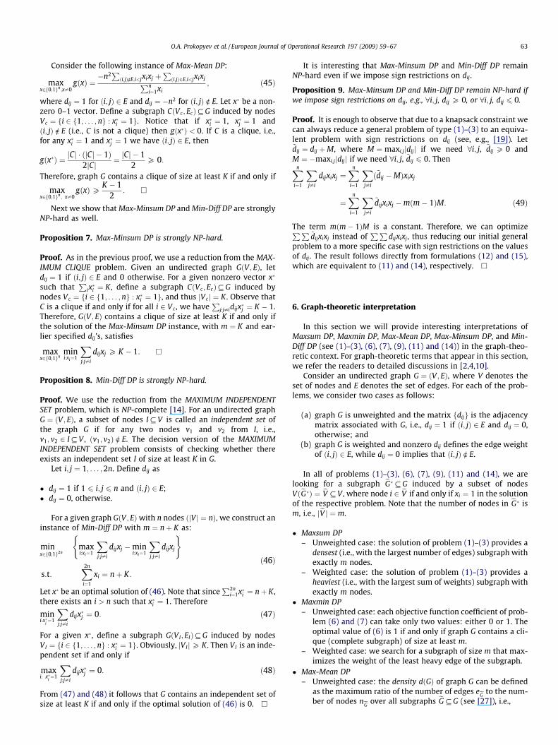
The first experiment is to compare the exact solution times forthe linear mixed integer programming reformulations of the fol-lowing four problems: Maxsum DP, Maxmin DP, Max-Minsum DP,and Min-Diff DP. All instances were solved using the CPLEX 9.0MIP solver with default parameters. We also imposed a 1 hour timelimit. The computational results are reported in Table 1.

7.3. Heuristic solution

The theoretical computational complexity results discussed inSection 5 indicate that the considered equitable dispersion prob-lems are difficult combinatorial optimization problems. Therefore,heuristic based algorithms can be applied in order to obtain good-quality solutions in a fast manner. Greedy Randomized AdaptiveSearch Procedure (GRASP) is a rather popular tool for solving Max-sum DP and Maxmin DP (see, e.g., [15,31]). Motivated by the successof GRASP in solving Maxsum DP and Maxmin DP, we implemented asimple GRASP-based heuristic for solving Max-Minsum DP, which isa somewhat similar problem.

GRASP is a metaheuristic procedure, proposed by Feo and Re-sende [13]. The main components of GRASP are the constructionand the improvement phases. In the construction phase, GRASPcreates a complete solution by iteratively adding components ofa solution with the help of a carefully designed greedy function,which is used to perform the selection. The improvement phasethen takes the incumbent solution and performs local perturba-tions in order to get a local optimal solution, with respect to some

O.A. Prokopyev et al. / European Journal of Operational Research 197 (2009) 59–67 65

predefined neighborhood. Different local search algorithms can bedefined according to the chosen neighborhood. Next, we briefly de-scribe the implementation details of the heuristic.

Construction Phase. Let Mk be a partial solution given by a set ofkð1 6 k < m) elements selected, that is exactly k variables are fixedto be 1. The initial set M1 is constructed randomly by selecting anindex i 2 f1; . . . ;ng. For any i 2 f1; . . . ;ng nMk, we introduce Df kðiÞas the marginal contribution made by element i toward Mkþ1 fromthe current partial solution Mk. Let

skðiÞ ¼Xj2Mk

dij:

Then, for Max-Minsum DP we define

Df kðiÞ ¼min minj2Mk

fskðjÞ þ djig; skðiÞ� �

� f ðMkÞ; ð54Þ

where f ðMkÞ is the value of the objective function with variablesfrom Mk fixed to 1.

Algorithm 1. Construction phase

input: coefficients dji for j ¼ 1; . . . ;n and i ¼ 1; . . . ;n and a con-stant noutput: a vector x 2 f0;1gn

/* initialize solution x*/x ð0; . . . ;0Þ; M1 random index from {1, . . .,n}for k 1 to m� 1 do

/* create a restricted candidate list (RCL) */L f1; . . . ;ng nMk

Table 1Exact solution time comparison (10 instances of each size)

Problem size TimenMeasure Maxsum

n ¼ 30m ¼ 10

Maximum 360.8 secondMedian 237.3 secondMinimum 105.6 second

n ¼ 30m ¼ 15

Maximum 327.3 secondMedian 232.1 secondMinimum 80.26 second

n ¼ 40m ¼ 10

Maximum P1 hourMedian P1 hourMinimum P1 hour

n ¼ 40m ¼ 15

Maximum P1 hourMedian P1 hourMinimum P1 hour

n ¼ 50m ¼ 10

Maximum P1 hourMedian P1 hourMinimum P1 hour

n ¼ 50m ¼ 15

Maximum P1 hourMedian P1 hourMinimum P1 hour

n ¼ 50n ¼ 20

Maximum P1 hourMedian P1 hourMinimum P1 hour

n ¼ 50m ¼ 25

Maximum P1 hourMedian P1 hourMinimum P1 hour

n ¼ 50m ¼ 30

Maximum P1 hourMedian P1 hourMinimum P1 hour

n ¼ 100m ¼ 10

Maximum P1 hourMedian P1 hourMinimum P1 hour

n ¼ 100m ¼ 12

Maximum P1 hourMedian P1 hourMinimum P1 hour

Order L according to function Df k as described inequation (54)

RCL first a elements of LSelect random index i 2 RCL; xi 1; Mkþ1 Mk [ fig

endreturn x

The GRASP algorithm uses a list of candidate components, alsoknown as the restricted candidate list (RCL). We sort the candidatevariables according to their marginal contribution Df kðiÞ to theobjective function. Then we select the first a indices to form theRCL. At each iteration of the construction phase, parameter a is arandom variable, uniformly distributed between 1 and jLj, the sizeof the set of variables to be fixed. One variable in the RCL israndomly selected at each iteration k P 1 with equal probability.It is then included into Mkþ1 and its value is set to 1. Theimplementation details of the construction phase are presentedin Algorithm 1.

Improvement phase. The improvement phase of GRASP has theobjective of finding a local optimal solution according to someneighborhood structure. The neighbors in our problem are ob-tained by perturbing the incumbent solution in the followingway. Two different variables xi and xj are selected and their valuesare exchanged so that

Pni¼1xi remains unchanged. After the pertur-

bation, the new solution is accepted if the objective is improved.Otherwise, another perturbation of the incumbent solution isperformed. This phase terminates after N iterations without any

Maxmin Max-Minsum Min-Diff

1.594 second 0.547 second 41.50 second0.953 second 0.352 second 34.14 second0.672 second 0.094 second 22.06 second

14.72 second 1.016 second 56.63 second5.969 second 0.602 second 42.53 second3.141 second 0.218 second 25.89 second

5.078 second 2.453 second 822.5 second3.704 second 1.430 second 682.0 second2.781 second 0.578 second 535.8 second

86.91 second 7.594 second 3226 second34.37 second 3.867 second 2678 second10.09 second 0.500 second 1447 second

23.53 second 4.125 second P1 hour12.92 second 3.516 second P1 hour6.468 second 1.688 second P1 hour

236.9 second 45.55 second P1 hour142.9 second 28.05 second P1 hour59.34 second 11.22 second P1 hour

1638 second 180.4 second P1 hour592.9 second 145.6 second P1 hour241.4 second 25.06 second P1 hour

P1 hour 481.0 second P1 hour3274 second 81.95 second P1 hour1376 second 10.73 second P1 hour

P1 hour 112.3 second P1 hourP1 hour 32.22s P1 hourP1 hour 17.63 second P1 hour

395.9 second 201.0 second P1 hour303.9 second 152.7 second P1 hour196.3 second 106.5 second P1 hour

1967 second 1019 second P1 hour1288 second 799.0 second P1 hour778.5 second 350.0 second P1 hour

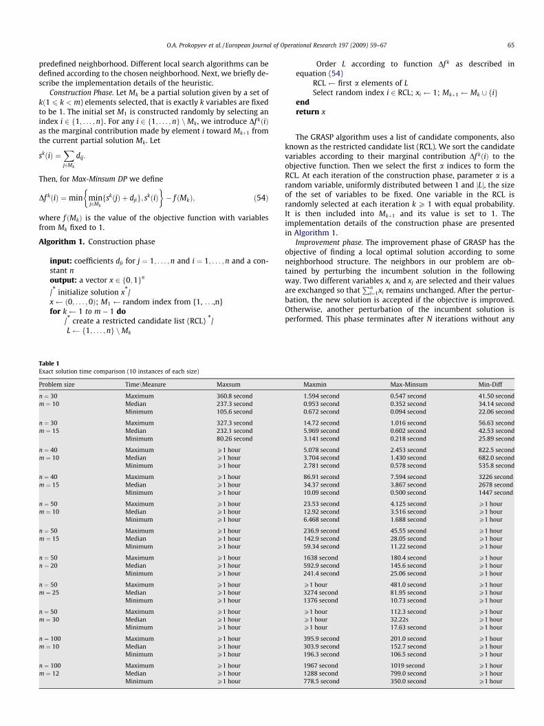
Table 2Computational results for solving Max-Minsum DP via GRASP

Problem size Time Exact solution total it ¼ 500 total it ¼ 1000

CPU (s) CPU (s) Gap (%) CPU(s) Gap (%)

n ¼ 50m ¼ 10

Maximum 4.125 2.281 0.757 3.875 0.757Median 3.516 1.869 0.218 3.502 0.012Minimum 1.688 1.653 0.076 2.841 0

n ¼ 50m ¼ 15

Maximum 45.546 4.564 1.507 8.712 0.905Median 28.047 3.594 1.002 6.670 0.611Minimum 11.219 3.008 0.598 6.111 0.296

n ¼ 50m ¼ 20

Maximum 180.36 5.453 1.616 12.034 1.029Median 145.64 5.064 0.981 10.33 0.613Minimum 25.062 4.492 0.460 8.100 0.279

n ¼ 50m ¼ 25

Maximum 481.03 8.620 1.669 15.469 1.441Median 81.952 7.243 1.393 13.115 0.796Minimum 10.734 6.237 0.828 11.767 0.237

n ¼ 50m ¼ 30

Maximum 112.30 10.318 1.1554 14.045 0.902Median 32.219 8.874 0.623 13.118 0.408Minimum 17.625 6.278 0.301 4.748 0.085

n ¼ 100m ¼ 10

Maximum 201.02 6.466 3.718 6.355 4.034Median 152.72 5.561 3.185 5.814 2.957Minimum 106.52 5.045 2.335 5.228 2.493

n ¼ 100m ¼ 12

Maximum 1019.5 8.280 5.003 16.767 3.871Median 798.98 7.150 3.700 14.457 3.165Minimum 349.99 6.977 2.653 12.406 2.478

66 O.A. Prokopyev et al. / European Journal of Operational Research 197 (2009) 59–67

improvement, where N is a given parameter in the algorithm. Inthe computational experiments reported below, we set N ¼ 100.

Termination criterion. The two-phase GRASP algorithm is set upto run until a fixed number of iterations total it is reached.

Results. The computational results of GRASP on Max-Minsum DPare given in Table 2. Since GRASP is a randomized algorithm, weran each instance 10 times and used the average heuristic subop-timal solution and CPU time to assess the performance.

7.4. Discussion

The first set of numerical experiments (see Table 1) was per-formed in order to compare relative difficulty of solving the MIPreformulations of two well-known measures (Sum and MinimumDispersion) and two new measures proposed in the paper (Minsumand Differential Dispersion). The reported computational results inTable 1 indicate that Maxsum DP and Min-Diff DP are the most chal-lenging problems; Max-Minsum DP seems to be the easiest one tosolve among the presented measures; and Maxmin DP is some-where in between. These results imply that in some situationswe may prefer the selection of a particular measure due to require-ments on the practical computational complexity of its respectivelinear mixed 0–1 programming formulation. The results maychange if we vary the density of the inter-element distance matri-ces and/or the distribution used to generate the matrices. However,we can conclude that our MIP reformulations can handle problemsonly of relatively modest size (around 100 variables) in a reason-able amount of time on a standard PC.

Results in the second set of numerical experiments (see Table 2)show good performance of GRASP-based heuristics for solving Max-Minsum DP, which confirms similar results obtained for Maxsum DPand Maxmin DP reported in the literature [15,31]. The implementedheuristic is rather simple, however it was able to provide reasonablygood solutions (about 3% optimality gap for largest problems) with afar better CPU time than the exact solution via CPLEX.

We also compared the solutions obtained via each measure.From our computational experiments, we conclude that the con-sidered measures do not agree in general although some maymatch with each other more and some others less. This impliesthat the efficiency-based measures sum and minimum do not usu-

ally provide equitable dispersion among elements. Hence, to en-sure an equitable system, we need to incorporate some equity-based measure. Our results also imply that to improve efficiencyand, more importantly, equity, the measure selection must bebased on the problem context as well as improvement require-ments. Often times, more effort should be made in interpretingthe equity results [36].

8. Conclusion

In this paper, we introduce three equity-based measures for thedispersion problem to address the imbalance of studying efficiencyand equity in the optimization literature. We believe the main con-tribution of the paper is to enhance our understanding of equity inthe optimization framework for the dispersion problems. We de-velop mathematical programs with proposed equity measuresbeing objectives and present several mixed-integer linear reformu-lations. Computational complexity and graph-theoretic interpreta-tion of these problems are studied.

The principles of the proposed equity measures can be appliedin many other optimization problems where the issue of equityamong various entities in the system must be addressed. As forsolution, we may improve the mixed-integer reformulations anddevelop more efficient exact and heuristic algorithms.

After establishing these equity measures, it would be interest-ing to study multi-objective optimization that attempts to balanceefficiency and equity. Efficiency and equity-based measures mustbe carefully selected [29]. In addition, the model should providea flexible and interactive way for decision makers to make thetradeoff between efficiency and equity. It would also be interestingto apply stochastic and robust discrete optimization to address theequity issue under the uncertainty of problem parameters.

Acknowledgments

The authors would like to thank the anonymous referees fortheir helpful comments. The research of the first two authors ispartially supported by the grant from AFOSR. The research of thefirst author is also supported by NSF grant CMMI-0825993.

O.A. Prokopyev et al. / European Journal of Operational Research 197 (2009) 59–67 67

References

[1] G.K. Adil, J.B. Ghosh, Maximum diversity/similarity models with extension topart grouping, International Transactions in Operations Research 12 (2005)311–323.

[2] R.K. Ahuja, T.L. Magnanti, J.B. Orlin, Network Flows: Theory, Algorithms, andApplications, Prentice-Hall, Upper Saddle River, NJ, 1993.

[3] S�. Agca, B. Eksioglu, J.B. Ghosh, Lagrangian solution of maximum dispersionproblems, Naval Research Logistics 47 (2000) 97–114.

[4] B. Bollobás, Modern Graph Theory, Springer, New York, NY, 1998.[5] I.M. Bomze, M. Budinich, P.M. Pardalos, M. Pelillo, The maximum clique

problem, in: D.-Z. Du, P.M. Pardalos (Eds.), Handbook of CombinatorialOptimization, vol. A, Kluwer Academic Publishers, Boston, MA, 1999, pp. 1–74.

[6] J.R. Brown, The knaspack sharing problem, Operations Research 27 (2) (1979)341–355.

[7] J.R. Brown, The sharing problem, Operations Research 27 (2) (1979) 324–340.[8] A. Caprara, D. Pisinger, P. Toth, Exact solution of the quadratic knapsack

problem, INFORMS Journal on Computing 11 (1999) 125–137.[9] F. Cheah, D.G. Corneil, The complexity of regular subgraph recognition,

Discrete Applied Mathematics 27 (1990) 59–68.[10] R. Diestel, Graph Theory, second ed., Springer, New York, NY, 2000.[11] E. Erkut, S. Neuman, Analytical models for locating undesirable facilities,

European Journal of Operational Research 40 (1989) 275–291.[12] E. Erkut, The discrete p-dispersion problem, European Journal of Operational

Research 46 (1990) 48–60.[13] T.A. Feo, M.G.C. Resende, Greedy randomized adaptive search procedures,

Journal of Global Optimization 6 (1995) 109–133.[14] M.R. Garey, D.S. Johnson, Computers and Intractability: A Guide to the Theory

of NP-Completeness, W.H. Freeman, New York, NY, 1979.[15] J.B. Ghosh, Computational aspects of the maximum diversity problem,

Operations Research Letters 19 (1996) 175–181.[16] F. Glover, C.-C. Kuo, K.S. Dhir, Heuristic algorithms for the maximum diversity

problem, Journal of Information and Optimization Sciences 19 (1998) 109–132.

[17] P. Hansen, I.D. Moon, Dispersing facilities on a network, Cah CERO 36 (1994)221–234.

[18] R. Hassin, S. Rubinstein, A. Tamir, Approximation algorithms for maximumdispersion, Operations Research Letters 21 (1997) 133–137.

[19] H. Huang, P. Pardalos, O.A. Prokopyev, Lower bound improvement and forcingrule for quadratic binary programming, Computational Optimization andApplications 33 (2006) 187–208.

[20] R.K. Kincard, Good solutions to discrete noxious location problems viametaheuristics, Annals of Operations Research 40 (1992) 265281.

[21] G. Kortsarz, D. Peleg, On choosing a dense subgraph, in: Proceedings of the34th IEEE Symposium on Foundations of Computer Science, Palo Alto, CA,1993, pp. 692–701.

[22] M.J. Kuby, Programming models for facility dispersion: The p-dispersionand maximum dispersion problems, Geographical Analysis 19 (1987) 315–329.

[23] C.-C. Kuo, F. Glover, K.S. Dhir, Analyzing and modeling the maximum diversityproblem by zero-one programming, Decision Sciences 24 (1993) 1171–1185.

[24] I.D. Moon, S.S. Chaudhry, An analysis of network location problems withdistance constraints, Management Science 30 (1984) 290–307.

[25] P.M. Pardalos, G.P. Rodgers, Computational aspects of a branch and boundalgorithm for quadratic zero-one programming, Computing 45 (1990) 141–144.

[26] P.B. Mirchandani, R.L. Francis (Eds.), Discrete Location Theory, Wiley,Hoboken, NJ, 1990.

[27] J.-C. Picard, M. Queyranne, A network flow solution to some nonlinear 0–1programming problems with applications to graph theory, Networks 12(1982) 141–159.

[28] D. Pisinger, Upper bounds and exact algorithms for p-dispersion problems,Computers and Operations Research 33 (2006) 1380–1398.

[29] M. Rahman, M.J. Kuby, A multiobjective model for locating solid waste transferfacilities using an empirical opposition function, Information Systems andOperations Research 33 (1995) 3449.

[30] S.S. Ravi, D.J. Rosenkrantz, G.K. Tayi, Heuristic and special case algorithms fordispersion problems, Operations Research 42 (1994) 299310.

[31] M.G.C. Resende, R. Marti, M. Gallego, A. Duarte, GRASP and path relinking forthe max–min diversity problem, Computers and Operations Research (2008),doi:10.1016/j.cor.2008.05.011.

[32] M. Tawarmalani, S. Ahmed, N.V. Sahinidis, Global optimization of 0–1hyperbolic programs, Journal of Global Optimization 24 (2002) 385–416.

[33] M.B. Teitz, Toward a theory of public facility location, Papers in RegionalScience 21 (1968) 35–51.

[34] R.R. Weitz, S. Lakshminarayanan, An empirical comparison of heuristicmethods for creating maximally diverse groups, The Journal of theOperational Research Society 49 (1998) 635–646.

[35] T.-H. Wu, A note on a global approach for general 0–1 fractional programming,European Journal of Operational Research 101 (1997) 220–223.

[36] H.P. Young, Equity: In Theory and Practice, Princeton University Press,Princeton, NJ, 1993.