8>'~WATER RESOURCES RESEARCH, YOLo 18, NO.3, PAGES 557-562, JUNE 1982

Numerical Treatment of Leaky Aquifers in the Short Time Range

BENITO CHEN AND ISMAEL HERRERA

Instituto de Investigaciones en Matematicas Aplicadas y en Sistemas, Universidad Nacional Autonoma de MexicoA. P. 20-726, Mexico City, Mexico

The numerical treatment of leaky aquifers in the short time range is complicated because it requiresthe use of very refined meshes. This range of time includes not only pumping tests but also manyregional studies because the definition of short time range depends on the thickness and diffusivity ofthe aquitard. The groundwater system of Mexico City is an example in which the short time rangeextends well beyond the whole life span of the pumping wells. In this paper a procedure which permitsthe avoidance, to a large extent, of these difficulties is explained; it is based on the integrodifferentialequations approach. In addition a method that can be applied to control the error is presented.

1. INTRODUCTION

Mathematically, leaky aquifers are characterized by theassumption of vertical flow in the aquitards, which is wellestablished for most cases of practical interest [Neuman andWitherspoon, 1%9a,b]. There are two main approaches forthe numerical modelling of systems of leaky aquifers: onewhich treats the basic equations in a direct manner withoutany further development [Chorley and Frind, 1978] and theother, which applies a transformation to obtain an equivalentsystem of integrodifferential equations [Herrera, 1976; Her-rera and Rodarte, 1973; Herrera and Yates, 1977; Hennartet al., 1981].

The latter procedure offers considerable computationaland analytical advantages [Herrera et al., 1980; Herrera,1976]. In the first approach the aquitard must be discretized,while in the integrodifferential approach the evolution of theaquitards is obtained by means of a series expansion [Herre-ra and Yates, 1977]. The accuracy in the first proceduredepends on the number and distribution of the nodes used inthe aquitard, while in the second one it depends on thenumber of terms used in the series expansion; the latter iseasier to control.

The treatment of leaky aquifers in the short time range isespecially delicate in connection with the facts mentionedabove. It is appropriate to say that the short time range isthat in which the aquitard can be approximated by a layer ofinfinite thickness [Hantush, 1960; Herrera and Rodarte,1973]. When the latter point of view is adopted, the defini-tion of the short time range depends on the error that one iswilling to accept. For example, if the admissible error for theapproximation of the aquitard behavior is 10%, then theshort time range is t' < 0.27, where t' is a dimensionless time(see the notation list at the end of the paper).

The relevance from the practical point of view of theperiod of operation to which we are referring can be betterappreciated by observing that the use of the term 'short timerange' may be misleading because the actual physical timecan be quite large. In the Mexico City area, for example,clays have exceptionally high specific storage; at TexcocoLake where artificial reservoirs have been built by inducingland subsidence [Herrera et al., 1974, 1977], there is a layerhaving a thickness of 32 m, a specific storage of 5.2 x 10-2

Copyright 1982 by the American Geophysical Union.

Paper number 2W0040.0043-1397/82/002W -0040$05.00

m-l, and a permeability of 0.47 x 10-3 mid. This implies aperiod of 83.8 yr for the short time range and thus the wholelife ~pan of the well field. In this example the specific storageis abnormally high, but the layer is not thick; what deter-mines the span of the short time range is the combination k'fSs'b,2 which in this case is 8.83 x IO-6fd. Cases for whichthis range is above 150 yr are not unusual; the Valley ofGuaymas, Mexico, is an example, but many more could becited.

The numerical modelling of the short time range is diffi-cult. One can understand the nature of such difficulties bylooking more carefully into the actual physical situation.When pumping starts in a main aquifer (Figure I), the effectsare first manifested there, and they slowly propagate into theaquitard. The short time range corresponds to that period oftime at which the total thickness of the aquitard is muchlarger than the part that has beeri affected by pumping. If auniform mesh were to be used on the whole aquitard, a veryrefined one would be required; thus too many nodes wouldbe introduced. This could be improved by the use of anonuniform mesh, but with such procedure it is necessary tohave a criterion for distributing the nodes and readjusting themesh as the time elapses, since the region of the aquitardaffected by pumping changes with time.

When the integrodifferential equation approach is used,these problems are reflected in the number of terms that arerequired in the series expansion of the memory functions.This article is devoted to present a procedure that avoids, toa large extent, these difficulties.

The method is based on the observation that in the shorttime range the response of the aquitard is approximately thesame as if the thickness of the aquitard is infinite, i.e., it doesnot depend on the actual thickness of the aquitard as long asthis is larger than a certain minimum. In the integrodifferen-tial approach this gives rise to a one-parameter family ofpossible representations for the memory functions, and aprocedure is given here to adjust that parameter in such amanner that the number of terms in the series expansion isdecreased to a minimum.

In addition an analysis of the error implied by the approxi-mations used for the memory function that is more completethan previous ones [Herrera and Yates, 1977] is carried out.This allows supplying a criterion which permits defining inadvance the number of terms required to obtain a givenaccuracy.

Examples of application to actual field situations aregiven. The results obtained for them exhibit substantial

557

558 CHEN AND HERRERA: NUMERICAL TREATMENT OF LEAKY AQUIFERS

z

tThe system of (1)-(4) is equivalent [Herrera and Rodarte,

1973] to the integrodifferential equation

b'//////ff////////~l~///// a ( as ) a ( as)-T- + -T-ax ax ay ay

K'b'

(' as.Jo at (x, y, t

subjected to

(5)

y/

"'"xFig. 1. A single leaky aquifer overlaid by one aquitard.

s(x, y, 0) = 0 (6)

When these equations are supplemented by suitable condi-tions in the boundaries limiting the horizontal extention ofthe region, one can obtain the drawdown s in the mainaquifer without computing the drawdown s' in the aquitard.When s' is required, however, it can be easily derived fromthe drawdown s [Herrera and Rodarte, 1973; Herrera andYates, 1977].

The melilory functionj{t') has two alternative representa-tions [Herrera and Rodarte, 1973]:

ao 1 ( ao )j{t') = 1 + 2 ~ e-n2,,:zt' = ~ 1 + 2 ~ e-n21t, (7)'" ('ITt')1/2n=l n=l

One can define an apparent storage coefficient Sa(t), whichchanges with time for a leaky aquifer. Consider (5) withouthorizontal flow; it is

as K' I t asS -+ --(t -'T)f(a'Tfh,2) d'T = Q (8)

at h' 0 at

Let the drawdown s(t) be a unit step function; i.e., it isinitially zero, and it is then suddenly increased to take thevalue 1, keeping it fixed thereafter. Then

as-(t) = 8(t) (9)at

where 8(t) is Dirac's delta function. By substitution of (9)into (8), one gets

reductions in the number of terms required for the seriesexpansions. In the worst case this number is 12, but it wouldhave been 128 if the transformation had not been used.

It seems worthwhile to recall that the same basic idea canbe used to simplify the numerical treatment of leaky aquifersin the short time range when the aquitard is discretized. Theargument presented here can be modified to produce acriterion for distributing the nodes and readjusting the meshused in the aquitard.

2. PRELIMINARY NOTIONS

Leaky aquifers are characterized by the fact that thepermeabilities of the semipervious layers (aquitards) sepa-rating the main aquifers (Figure I) are very small. When thecontrast of permeabilities between the main aquifers and theaquitards is one order of magnitude or more, the flow can betaken as vertical in the aquitards [Neuman and Witherspoon,1969a,b].

To be specific, we restrict attention to the case of onemain aquifer limited above by one aquitard and overlying animpermeable bed (Figure I). The analysis is applicable,however, to a multiaquifer system in the short time rangebecause in this range the interaction between the mainaquifers is not perceptible. Also, if the main aquifer overlaysanother aquitard, the modification of the arguments isstraightforward [see, for example, Herrera, 1970].

The governing equation when the aquitard is homoge-neous is

(10)

and the total yield given by the system aquifer-aquitard is

I t K' ItQ(T) dT = S + ~ !(a'Tlb'Z) dT = S + S'F(a'tlb'1

0 b 0

a ( as ) a ( as ) as' as -T- + -T- + K' -(0, t) + Q = S-

ax ax ay ay az at

in the aquifer and

(11)(1)

where F is given by

F(t') = f:'!(T)dT (12)

It is natural to define the apparent storage coefficient Sa ofthe aquifer-aquitard system as the total volume of water perunit area yielded by the system under a unit decline ofpiezometric head. Hence

Sa(t) = J: Q(T) dT = S + S'F(a'tlb'1 (13)

which is an increasing function of the time elapsed since the

CHEN AND HERRERA: NUMERICAL TREATMENT OF LEAKY AQUIFERS 559

dominates the error, in contrast toapplication of the unit decline of piezometric head. If there isno aquitard, S' = 0 and Sa(t) = S, which is independent oftime and exhibits the consistency of our definition.

Since f(t') is defined by an infinite series, it is desirable toobtain a good approximation for F(t') using only a smallnumber of terms. We consider two possible approximations.The first is to truncate

00 f t' F(t') = t' + 2 n~1 0 e-n2.,z,. dT

(14)

to N terms:

N f l' F~t') = t' + 2 n~1 0

2 i r.~. e-n2..z,. d'T

e-n',,;zT dT = F(t']

-2 if:' e-n'"" dT (15)n=N+\

The second [Herrera and Yates, 1977] is to integrate (14)first, sum exactly one of the resulting series, and truncate theother one. This can be obtained observing that

r (i ~ \n=\

3. APPROXIMATION OF THE ApPARENT STORAGE

COEFFICIENT

From (7), it follows that for every () > 0

001 + 2 ~ e-(n'/9f

n=1

.f( 8f') = "(;8t~

2F(t') = t' --:2n2

00 1

-~2 nn=1

(20)~

+ 2 ~ e-n2,,:zlJt'n=1

=

(16)

Furthermore, define00

+ 2 ~ e-n2ft'n;=1

d(t') =Define (21)

Then(17)

(22)

Hence

f(t') = v'i[l + 15(8, t')]f(8t') (23)

where

~

d(t')

d(8t')«X8, t') = (24)

From (23) it follows that

F(t') = (J-I/2F«(Jt') + ~«(J, t') (25)

+ 2 iJ oo e-n2";,. dT (18)

n=N+1 "

The initial value F ~O), which is different from zero, hasbeen denoted as AN by Herrera and Yates [1977]. This is

I 2NI 2001AN = F ~O) = ---~ -= -~ -3 1T2 n2 1T2 n2

n=1 n=N+1

Of the two approximations, (15) and (17), the second oneyields better results. First, for any N it preserves total yield[see Herrera and Yates, 1977]. Second, we are only truncat-ing

(19)where f t'

6.(6, t') = V6 0c5(fJ, ,,)f(fJ,,) d" (26)

A bound for ~ can be obtained when a bound for c5 is knownIndeed, ife-n2",J-t'

n2

~

~n=N+! IlXfJ, T)I oS 61 0 oS T oS t' (27)

thenwhich converges very quickly for positive t'. In (15) theseries 1.1(8, t')1 ~ El 8-1/2F(8t') (28)

In numerical applications of the integrodifferential ap-proach [Herrera and Yates, 1977; Hennart et al., 1981] thefirst of the series expansions given in (7) is used. Equation

2 ~

~n=N+\n2

n=N+\ Jill

and it diminishes rapidly for further time steps. So it is veryeasy to control the error for any time t'. The same is not truefor (15), where the error increases with time.

m -1/2 ~f( £Jt') -(J d( £Jt')

560 CHEN AND HERRERA: NUMERICAL TREATMENT OF LEAKY AQUIFERS

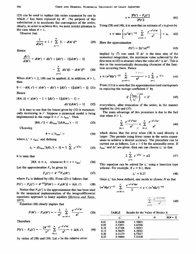
(23) can be used to replace this series expansion by one inwhich t' has been replaced by 8t'. The purpose of thissubstitution is to accelerate the convergence of the series;clearly, in order to achieve this, we must restrict attention tothe case when 8> 1.

Observe that

IF(I') -Fa(I')1e = IF(I')I (41)

Using (28) and (40), it is seen that an estimate of e is given by{ '" -n2,,:z8t' -

e S max (71"391')-112 ~ Tn=N+l

Here the approximation

F(I') = 2(1'/71")112 (43)

implied by (7) was used. If ~I' is the time step of thenumerical integration, the maximum value achieved by thefirst term in (42) is attained when the value of I' is ~I'. This isdue to the monotonically decreasing character of the func-tion occurring there. Hence

-n2,,:z84t' ,e --, -'" .

(42)+ £1

~

= 1 + ~ [1 -d(/Jt,)]mm=!

(29)1

d(6t')

Hence

d(t')

d( 81')= d(8t') -d(t') + [d(t') -1][d(8t') -1]

w ~

£ S (~8I1.t')-I/2 ~ 2 + 2 ~ e-n"llc in

n=N+1 n=1

From (13) it is seen that the approximation used correspondsto replacing the storage coefficient S' by

( t ' )1/2 S' ~ < S' (45)

everywhere, after truncation of the series, in the mannerimplied by (34) and (37).

The main advantage of this procedure is due to the factthat when 8> 1,

~ -n2.19~t' ~ -n2.1~t'e e~<~n2 n2N+I "-': N+I

which shows that the error when (18) is used directly islarger. This permits using fewer terms in the series expan-sions to achieve a desired accuracy. The procedure can becarried out as follows. Let £ > 0 be the admissible error. Iftmax' and I1.t' are given, then one can choose tc' so that

~2 ~ e-n2ltc' = £/2

n=1

This equation can be solved for tc' using a bisection typescheme. For example, if £ = 0.1, then

tc' = 0.27 (48)

Once tc' has been defined, one needs to choose N so that'" -n2.1941'(1T38I1.t,)-1/2 ~ e

n=N+1

(44)

00

-~ d(t')[1 -d(8t')]m (30)m=2

When d(8t') < 2, (30) can be applied; if, in addition, 9> I,then

0 < -cX9, t') < d(9t') -d(t') + [d(t') -1][d(8t') -I] (31)

Hence

IcX9, t)1 < d(8t') -1 -+- [d(t') -1][d(8t') -I] =

d(t')[d( 8t') -I] (32)

It is easy to see that the bound given by (32) is monotoni-cally increasing in t'. Suppose a numerical model is beingimplemented in the range 0 :S t' :S tmax'. Then

IcX9, t')1 < d(tmax')[d(8tmax') -I] (33)(46)

Choosing(J = tc'/tmax' >

where tc' > tmax' and defining

(34)

~

£1 = d(tmax')[d(tc') -IJ = 2 ~ e-n2/tc' (35)

(47)

< E < (1T366.t,)-I/22

(49)

it is seen that

IcX6, '1") :S 101 whenever 0 < 'I" < tmax' (36)

Let the approximation Fa be given by

Fa(t') = 6-112FM81') (37)

where F N is defined by (18). From (25) it follows that

F(t') -F a(t') = 6-112[F( 81') -F M 81')] + d( 6, I') (38)

Notice that F Mt') is the approximation that has been usedin the numerical implementation of the integrodifferentialequations approach to leaky aquifers [Herrera and Yates,1977].

Equation (18) clearly implies that-2 2e n 8"

n2

2 00

F(8t') -FNf.8t') = --~11'2

n=N+1(39) TABLE Results for the Valley of Mexico A

t 'c (J N N(8 = 1)

Therefore 0.010.050.100.150.200.25

0.166900.228210.271080.304550.333790.36064

3.388224.632685.503126.182626.776177.32118

28-112 00 e-n2".J.lJt'

F(t') -Fa(t') = -~ ~ 2 + 11(8, t')'IT n

N+l

by virtue of (38) and (39). Let E be the relative error:

(40)

CHEN AND HERRERA: NUMERICAL TREATMENT OF LEAKY AQUIFERS 561

TABLE 2. Results for the Valley of Mexico B TABLE 4. Results for an Aquifer With Fictitious Properties

0.010.050.100.150.200.25

0.166900.228210.271080.304550.333790.36064

3.388224.632685.503126.182626.776177.32118

4. NUMERICAL EXAMPLES

Two of the leaky aquifers that have been extensivelystudied in Mexico are the ones under the Valley of Mexico[Herrera et al., 1974, 1977] and Guaymas. The differentproperties of the aquifers have a wide range of variation.

To exemplify the efficiency of the procedure we have usedtwo sets of values from the Valley of Mexico that weconsider to be representative, one set from Guaymas andanother from an aquifer with ficticious properties.

For each aquifer the computations were done for both the(J 'optimum' given by (34) and for (J = 1 for a wide range ofrelative errors. A result with a relative error of 10% isusually very satisfactory. The results are presented below.

Valley of Mexico A (Table 1):

S' = 4.8 T' = 1.816 X 10-5 km2/yr

h' = 4.8 X 10-2 km tmax = 30 yr ~t = 0.5 yr

or in nondimensional form

tmax' = 4.926 X 10-2 ~t' = 8.210 x 10-4

Valley of Mexico B (Table 2):

S' = 2.4 T' = 3.333 X 10-6 km2/yr

h' = 2.4 X 10-2 km tmax = 30 yr ~t = 0.5 yr

tmax' = 7.226 X 10-2 ~t' = 1.200 X 10-3

Guaymas (Table 3):

S' = 0.75 T' = 1.230 X 10-7 km2/yr

h' = 7.5 X 10-2 km tmax = 50 yr ~t = 0.5 yr

tmax' = 1.457 X 10-3 ~t' = 1.457 X 10-5

Aquifer with ficticious properties (Table 4):

S' = 4.0 T' = 3.1536 X 10-6 km2/yr

h' = 1.0 X 101 km tmax = 30 yr ~t = 0.5 yr

tmax' = 2.365 X 10-3 ~t' = 3.942 X 10-5

NOTATION

AN = (2/71) ~n=N+I~ n-2h' thickness of aquitard, L.

d(t') function defined by (21).

f(t') memory function, equal to 1 + 2 ~n=)~ e-n2.,:z".F(t') = J 0" f( T) dT

F a(t') approximation of F(t'), defined by (37).F Nl.t') approximation of F(t'), defined by (38).

K' permeability of aquitard, LIT.Q(t') pumping rate from aquifer, J;.IT.

$ drawdown in aquifer, L.$' drawdown in aquitard, L.S storage coefficient of aquifer.

S' storage coefficient of aquitard.Sa(t) apparent storage coefficient of system, defined

by (13).t time, T.

t' dimensionless time, equal to a'tlb,2.tc' upper bound of short time range.

tmax' maximum value of t'.T transmissibility of aquifer, L2IT.

T' transmissibility of aquitard, L 21T.x, y, z coordinates, L.

a' = T'IS', L2IT.

15(t') Dirac's delta function.15(fJ, t') function defined by (24).d(fJ, t') function defined by~26).

I:: relative error, defined by (41).1::) error defined by (27).fJ positive parameter of the family of approxima-

tions Fa.

Acknowledgments. This paper was presented by invitation atthe John Ferris Symposium at the Spring Annual Meeting, AGU,Baltimore, Maryland, May 25-29, 1981.

0.166900.228210.271080.304550.333790.36064

3.388224.632685.503126.182626.776177.32118

REFERENCESChorley, D. W., and E. O. Frind, An iterative quasi-three-dimen-

sional finite element model for heterogeneous multiaquifer sys-tems, Water Resour. Res., 14(5), 943-952, 1978.

Hantush, M. S., Modification of the theory of leaky aquifers, J.Geophys, Res., 65(11), 3713-3725, 1960.

Hennart, J. P., R. Yates, and I. Herrera, Extension of the integrodif-ferential approach to inhomogeneous multiaquifer systems, WaterResour. Res., 17(4), 1044-1050, 1981.

Herrera, I., Theory of multiple leaky aquifers, Water Resour. Res.,6(1),185-193,1970.

Herrera, I., A review of the integrodifferential equations approachto leaky aquifer mechanics, paper presented at the Symposium onAdvances in Groundwater Hydrology, Am. Water Resour. As-soc., Minneapolis, Minn., 1976.

Herrera, I., and L. Rodarte, Integrodifferential equations for sys-tems of leaky aquifers and applications, I, The nature of appro xi-mate theories, Water Resour. Res., 9(4), 995-1005, 1973.

Herrera, I., and R. Yates, Integrodifferential equations for systemsof leaky aquifers, 3, A numerical method of unlimited applicabil-ity, Water Resour. Res., 13(4), 725-732,1977.

Herrera, I., J. Alberro, J. L. Le6n, and B. Chen, Analisis deasentamientos para la construcci6n de los lagos del plan Texcoco,Rep. 340, Inst. de Ing., Univ. Nac. Auton. de Mex., Mexico City,1974.

Herrera, I., J. Alberro, R. Graue, and J. J. Hanel, Development of

562 CHEN AND HERRERA: NUMERICAL TREATMENT OF LEAKY AQUIFERS

Neuman, S. P., and P. A. Witherspoon, Transient flow of groundwater to wells in multiple aquifer systems, Geotech. Eng. Rep. 69-1, Univ. of Calif., Berkeley, Jan. 1969b.

(Received June 24, 1981;revised December 15, 1981;

accepted December 22, 1981.)

artificial reservoirs by inducing land subsidence, IAHS-AISHPubl. 121, 39-45, 1977.

Herrera, I., J. P. Hennart, and R. Yates, A critical discussion ofnumerical models for multiaquifer systems, Advan. Water Re-sour., 3(4), 159-163, 1980.

Neuman, S. P., and P. A. Witherspoon, Theory offtow in a confinedtwo-aquifer system, Water Resour. Res., 5(4), 803-816, 1%9a.