The Taylor–Melcher leaky dielectric model as a macroscale ...

Under consideration for publication in J. Fluid Mech. 1

The Taylor–Melcher leaky dielectric modelas a macroscale electrokinetic description

ORY SCHNITZER† AND EHUD YARIV

Department of Mathematics, Technion - Israel Institute of TechnologyHaifa 32000, Israel

(Received 21 April 2015)

While the Taylor–Melcher electrohydrodynamic model entails ionic charge carriers, itaddresses neither ionic transport within the liquids nor the formation of diffuse space-charge layers about their common interface. Moreover, as this model is hinged uponthe presence of nonzero interfacial-charge density, it appears to be in contradiction withthe aggregate electro-neutrality implied by ionic screening. Following a brief synopsispublished by Baygents & Saville (Third International Colloquium on Drops & Bubbles,vol. 7, 1989, p. 7) we systematically derive here the macroscale description appropriatefor leaky dielectric liquids, starting from the primitive electrokinetic equations and ad-dressing the double limit of thin space-charge layers and strong fields. This derivationis accomplished through the use of matched asymptotic expansions between the narrowspace-charge layers adjacent to the interface and the electro-neutral bulk domains, whichare homogenized by the strong ionic advection. Electrokinetic transport within the elec-trical ‘triple layer’ comprising the genuine interface and the adjacent space-charge layersis embodied in effective boundary conditions; these conditions, together with the simpli-fied transport within the bulk domains, constitute the requisite macroscale description.This description essentially coincides with the familiar equations of Taylor & Melcher(Annu. Rev. Fluid Mech., vol. 1, 1969, p. 111). A key quantity in our macroscale de-scription is the ‘apparent’ surface-charge density, provided by the transversely-integratedtriple-layer microscale charge. At leading order, this density vanishes due to the expectedDebye-layer screening; its asymptotic correction provides the ‘interfacial’ surface-chargedensity appearing in the Taylor–Melcher model. Our unified electrohydrodynamic treat-ment provides a reinterpretation of both the Taylor–Melcher conductivity-ratio param-eter and the electrical Reynolds number. The latter, expressed in terms of fundamentalelectrokinetic properties, becomes O(1) only for intense applied fields, comparable withthe transverse field within the space-charge layers; at this limit, however, the asymp-totic scheme collapses. Surface-charge advection is accordingly absent in the macroscaledescription. Because of the inevitable presence of (screened) net charge on the genuineinterface, the drop also undergoes electrophoretic motion. The associated flow, however,is asymptotically smaller than that corresponding to the the Taylor–Melcher circulation.Our successful matching procedure contrasts the analysis of Baygents & Saville (1989),who considered more general electrolytes and were unable to directly match the innerand outer regions. We discuss this difference in detail.

1. Introduction

The Taylor–Melcher leaky dielectric model describes electrohydrodynamic phenom-ena in poorly conducting liquids. In this model, volumetric charge is completely absent.

† Present address: Department of Mathematics, Imperial College London, South KensingtonCampus, SW7 2AZ, London, United Kingdom

2 O. Schnitzer and E. Yariv

The liquids are described as dielectric materials that nonetheless possess finite Ohmicconductivities; this description reflects Taylor’s realisation (1966) that, however smalltheir conductivity is, poorly conducting liquids are fundamentally different from per-fect dielectrics. Specifically, rather then satisfying the interfacial condition of electric-displacement continuity, pertinent to dielectric liquids, the electric-field distribution isset at steady state by the condition of electric-current continuity. With the inevitablejump in the electric displacement, the field distribution satisfying the latter conditionis generally accompanied by a nonzero surface-charge distribution at the interface. Theelectrical shear forces acting on the charged interface then give rise to fluid motion.The model put forward by Taylor (1966) in the context of electrohydrodynamic drop

deformation was revisited by Melcher & Taylor (1969), and has since been the basisfor numerous investigations in electrohydrodynamic phenomena (Feng & Scott 1996;Feng 1999; Craster & Matar 2005; Salipante & Vlahovska 2014). The interfacial current-continuity condition was generalized to account for surface convection of charge, whoserelative magnitude is quantified by the electric Reynolds number. Taylor’s analysis, wheresurface convection is neglected, thus corresponds to low values of this dimensionlessgroup. In this limit, and for a specified interface geometry, the electrostatic problemis decoupled from the flow, satisfying a linear problem. This allows for straightforwardanalytic solutions.The charge carriers in the leaky dielectric model are accounted for only through the

prescription of (uniform) liquid conductivities. Thus, the Taylor–Melcher scheme avoidsthe need to account for ionic transport — a nonlinear mechanism underlying electroki-netic phenomena (Saville 1977). Analysis of leaky dielectric and electrokinetic flows havetherefore evolved more-or-less independently, with the two scientific communities beingessentially foreign.Since the charge carriers in leaky dielectric liquids are typically ions (Saville 1997), a

troubling question arises. It is well known that the presence of charged interfaces in anion-carrying liquid results in the formation of adjacent diffuse (‘Debye’) layers, within theliquid, of charge opposite to that on the interface. Since the Taylor–Melcher model doesnot allow for volumetric charges, these two layers are absent in it. Moreover, it is not apriori evident whether the surface-charge density appearing in the Taylor–Melcher modelmay be viewed as a coarse-grained aggregate quantity, namely the ‘apparent’ charge ofthe combined triple-layer system: after all, one might actually expect that this apparentcharge would vanish by screening.This paradox, along with additional ambiguities in the Taylor–Melcher model, empha-

sizes the need for a unified electrohydrodynamic approach, starting from the fundamentalelectrokinetic description. Our goal is to address this challenge in the context of Taylor’sclassical problem: a spherical drop in a uniform field. To account for the passage of cur-rent through the drop interface, as postulated by Taylor, the physicochemical model ofthe interface must allow for sorption of the charge carriers — here being simply the saltions. By applying an asymptotic limit which properly represents ‘leaky dielectric liquids,’a systematic analysis would reveal whether the Taylor–Melcher model indeed emerges.Since leaky dielectric liquids are poor conductors, their microscale description typi-

cally involves small ionic concentrations. Saville (1997) provides the characteristic value10−7 m for the corresponding Debye thickness (see (4.7)). In electrokinetic phenomenainvolving colloidal particles, this estimate is easily comparable with particle size; whenconsidering drops, however, which can reach millimeters in size, this estimate actuallysuggests considering the limit where the ratio δ of Debye thickness to drop size is ex-ceedingly small. This asymptotic limit has been extensively studied in the context ofelectrokinetic phenomena involving solid particles (Morrison 1970; Derjaguin & Dukhin

Leaky dielectric model as a macroscale electrokinetic description 3

1974; O’Brien 1983; Anderson 1989; Schnitzer & Yariv 2012a), ion-selective granules(Ben, Demekhin & Chang 2004; Yariv 2010), metal drops (Ohshima, Healy & White1984; Schnitzer, Frankel & Yariv 2013a), and gas bubbles (Schnitzer, Frankel & Yariv2014).Another fundamental parameter appearing in the electrokinetic problem is the ratio

β of the drop-scale voltage associated with the applied field and the thermal voltage (≈25 mv), see (4.35). For electrokinetic phenomena about small colloidal particles, Saville(1977) provides the typical value 5×10−4 for β. This estimate assumes a particle of radius0.1 µm in a field of magnitude 10 V cm−1; electrokinetic effects are observed also withslightly larger particles and stronger fields allowing for β = O(1). Much larger β valuesare found for drops in leaky dielectric fluids. These large values of the dimensionless fieldare not only due to the large length scales, but also due to the strong fields which aretypically applied. Thus Saville (1997) provides the typical figure 103 corresponding to adrop of millimetric size exposed to an electric field of magnitude 103 Vcm−1. The limitδ ≪ 1 must therefore be accompanied by the limit β ≫ 1.The above twofold limit was first employed in a short synopsis by Baygents & Saville

(1989). Specifically, Baygents & Saville (1989) considered the limit

1 ≪ β ≪ 1/δ, (1.1)

and applied it to a relatively standard electrokinetic model, where the microscale trans-port of ions through the interface is modelled through simple sorption kinetics. (For theabove mentioned scenario of a millimetric drop in a strong electric field, (1.1) requiresa Debye length ≪ µm.) The fluid domain was asymptotically decomposed into ‘inner’diffuse-charge layers, of O(δ) thickness, and ‘outer’ bulk regions, which are homogenizedby the intense ionic advection. Baygents & Saville (1989) were unable to directly matchthe inner and outer regions, and suggested that a separate analysis of an intermediatelayer, of thickness 1/β, is required. The resulting matching procedure, however, is notprovided in that concise synopsis, nor is the consequent macroscale description. Baygents& Saville (1989) do provide the eventual flow field, which is the same as that calculatedby Taylor (1966).In the present paper we revisit the Baygents–Saville approach. We employ the same

microscale electrokinetic model used by Baygents & Saville (1989), which for the purposeof brevity and clarity is here limited to binary electrolytes. In this case, we do manageto match the inner and outer regions, and thereby obtain a macroscale ‘coarse-grained’description, where the Debye-layer physics appear as effective boundary conditions. Thisdescription closely resembles the equations outlined by Melcher & Taylor (1969), but withseveral important differences. These include the absence of charge convection, the re-interpretation of the conductivity-ratio parameter of Taylor (1966), and the appearanceof electrophoretic drop motion at a higher asymptotic order.Our paper is constructed as follows. Following a physical description of the problem

in §2, we provide in §3 intuitive arguments, describing how coarse graining an electroki-netic model can give rise to a leaky-dielectric-type model. We then shift to a systematictreatment of the problem, formulating in §4 a microscale problem using the ab ini-

tio electrokinetic description, following Baygents & Saville (1989). In §5 we apply theBaygents–Saville limit (1.1), and derive the outer-bulk description. The diffuse-chargelayers are described and analysed at leading order in §6. The analysis of the subsequentasymptotic order is carried out in §7, where an asymptotic matching procedure providesthe requisite effective boundary conditions. The resulting macroscale model is recapit-ulated in §8 using the familiar leaky dielectric scaling. In §9 we discuss the surprisingdifferences between our analysis and those in the synopsis of Baygents & Saville (1989).


We conclude in §10, discussing at length the unique features of the macroscale descriptionwe obtain, and in particular the differences with the Taylor–Melcher model.To the best of our knowledge, the work of Baygents & Saville (1989) is the only attempt

to derive the equivalent of Taylor–Melcher model from the more primitive electrokineticdescription using the limit process appropriate for describing leaky dielectric liquids.Our analysis, which succeeds in deriving such a macroscale model, provides a major steptowards a unified treatment of electrohydrodynamics.

2. Physical problem

We consider essentially the same physicochemical problem as Baygents & Saville(1989), motivated by the prototypic problem addressed by Taylor (1966). An immiscibleliquid drop of radius a∗ (dimensional quantities are decorated hereafter with an asterisk)is suspended in another liquid. The viscosity and dielectric permittivity of the suspend-ing liquid are respectively denoted µ∗ and ǫ∗; consistently with the original notation ofTaylor (1966), the viscosity and dielectric permittivity of the suspended drop are respec-tively denoted µ∗/M and ǫ∗/S. For simplicity we consider symmetric electrolytes withionic valencies ±z; the two ionic species then possess an identical equilibrium concen-tration (say C∗) at large distances away from the drop. The ionic diffusivites of cationsand anions within the suspending liquid are respectively denoted D±

∗ ; in view of theEinstein–Smoluchowski relation, the respective diffusivities within the drop are MD±

∗ .As in Baygents & Saville (1989), passage of current through the interface is made possibleby assuming that the ions undergo sorption there. Specifically, we employ the simplestpossible model of fast reactions, where the excess-surface concentration is proportionalto that in the solution.A uniform and constant Electric field of magnitude E∗ is externally applied. Our interest

is in the steady-state flow which is reached in a reference frame co-moving with the drop.As in Taylor (1966), we assume that capillary forces are strong enough so the dropremains approximately spherical.The only difference between the preceding problem and that considered by Baygents

& Saville (1989) is the limitation to a binary electrolyte.

3. Intuitive overview

It is useful to precede the detailed asymptotic treatment provided in the next sectionswith an intuitive outline of some of the main results. In what follows, we employ heuristicassumptions and gross approximations; all these are clarified and substantiated in thesystematic analysis appearing in the following sections.As explained in §2, we assume sorption kinetics in the physicochemical model of the

interface, so as to allow for the passage of current. An inevitable consequence of thatmodel is the existence of interfacial charge, even in the absence of an applied field. This‘equilibrium’ charge is screened by two diffuse-charge layers on both sides of the interface.Their characteristic thickness 1/κ∗ is assumed thin compared with drop size a∗. Followingstandard electrokinetic descriptions in the thin-double-layer limit (Schnitzer & Yariv2012a) it is expected that the ions in the two diffuse layers are Boltzmann distributedwith the electric potential satisfying the one-dimensional Poisson–Boltzmann equations;this triple-layer structure trivially generalizes the familiar Gouy–Chapman structure ofthe electrical double layer. Using traditional notation we denote the potential difference,at equilibrium, between the interface and the outer edges of the external and internaldiffuse-charge layers by ζ∗ and ζ∗, respectively. These are of the order of the thermal


genuine interface

diffuse layers

Taylor–Melcher interface

bulk electrolyte homogenized by strong advection

∝ c∗E∗

∝ c∗E∗

apparent surface charge

current

electric displacement

S−1

ǫ∗E∗

ǫ∗E∗

τ

τ

electrical force

shear stress

electro-osmotic flow

interfacial electrical stress

dominant electrohydrodynamic

flow

∝ E∗

∝ Λ∗E∗

∝ Λ∗E2

∗

Λ∗

Figure 1. Schematic accompanying the intuitive overview of §3. Description from right to left: (i)Asymmetric ionic sorption implies an ‘equilibrium’ interfacial charge, screened by two adjacentdiffuse layers. Sorption also allows electric currents associated with the applied field to passthrough the compound Taylor–Melcher interface, while resulting in only a slight perturbationto the triple-layer structure. (ii) Gauss law on the depicted control-volume reveals that theperturbed triple layer deviates from electro-neutrality. The overall, or apparent, charge per unitarea is Λ∗. (iii) The tangential field is approximately uniform on the Debye scale. Its actionon the apparent charge, itself induced by the field, results in a macroscopic stress jump whichdrives the dominant flow field. (iv) The action of the field on the equilibrium charge distributionresults in steep electro-osmotic flow profiles. While this flow, and the macroscopic slip it entails,is relatively weak, the viscous shear inflicted on the microscopic interface is strong. It is exactlybalanced by the interfacial electric stress associated with the equilibrium surface-excess ionconcentration.

voltage ϕ∗ = k∗T∗/ze∗ (k∗T ∗ being the Boltzmann temperature and e∗ the elementarycharge). We consider the limit where applied field is large compared with thermal scaleϕ∗/a∗ but is nonetheless small compared with the transverse field in the narrow Debyelayers, which is of order κ∗ϕ∗:

ϕ∗

a∗≪ E∗ ≪ κ∗ϕ∗. (3.1)

This assumption is represented by the Baygents–Saville limit (1.1) mentioned above.We start with the effect of the applied field on the bulk liquid domains lying outside

the two diffuse-charge layers. These domains are approximately electro-neutral, with thecation and anion concentrations being nearly identical. The ionic concentration is uniformfar away from the drop. In principle, concentration polarization on the drop scale mayby triggered by effective ‘surface’ currents which originate at the Debye-scale transport.The extent and topology of such concentration non-uniformities are determined by abalance between diffusion and advection by the field-induced flow, characterised by thevelocity scale U∗. With the applied field assumed strong, it is plausible that the flow isstrong as well, in the sense that the Peclet number Pe = a∗U∗/D∗ is large, D∗ being acharacteristic diffusivity. Thus, the ionic concentration is dominated by advection, andpossesses uniform values in the external and internal bulk domains. The concentrationvalue in the suspending liquid is simply given by the far-field concentration, namely c∗; thedrop concentration, say c∗, is generally different. Thus, bulk concentration polarization


effects, often important in electrokinetic analyses (Chu & Bazant 2006; Mani & Bazant2011; Schnitzer et al. 2013b), are here prevented by the dominance of advection. Theconcentration deviations triggered by Debye-scale fluxes are confined to thin diffusivelayers where the concentration deviations from the respective bulk values are small.It follows that the bulk fluid domains can be regarded as ‘Ohmic’ media of uniformconductivities. In particular, the current density in the external bulk domain is, usingthe Einstein–Smoluchowski relation,

z2e2∗(D+∗ +D−

∗ )

k∗T ∗c∗E∗, (3.2)

where E∗ denotes the local electric field. The current density in the internal bulk domainis similar, with Mc∗E∗ replacing c∗E∗, E∗ denoting the local field value.With the Ohmic form (3.2), charge conservation in the bulk implies that the electric

potentials of the conservative fields E∗ and E∗ satisfy Laplace’s equation. To obtain ap-propriate boundary conditions, we consider the conservation of charge in an infinitesimalslab-shaped control volume spanning the triple layer. Assuming that the contribution oftangential advection is small, we obtain an equality of radial bulk currents

c∗E∗ · er ≈Mc∗E∗ · er, (3.3)

where the fields E∗ and E∗ are evaluated at the outer edges of the external and inter-nal diffuse layers, respectively, and er is a unit vector in the radial direction. Assumingfurthermore that the tangential component of the electric field is approximately transver-sally uniform across the triple layer, we find that the tangential component of the bulkfield is continuous across the ‘macroscale interface.’ Condition (3.3), in conjunction withthat continuity condition, serves to uniquely determine the bulk electric fields. Upon iden-tifying Mc∗/c∗ with the conductivity ratio R, these are the same as the fields calculatedby Taylor (1966).Since the applied field is assumed small compared with the Debye-layer field, the

perturbation to the equilibrium Debye cloud due to passage of current is small. Thisperturbation however is crucial since it results in a nonzero transversely-integrated triple-layer charge: it is the action of the applied field on this ‘apparent’ non-equilibrium surfacecharge that gives rise to the dominant flow field. Indeed, applying the integral form ofGauss law to the same slab-shaped control volume yields the apparent charge

Λ∗ ≈ ǫ∗E∗ · er − S−1ǫ∗E∗ · er, (3.4)

which is generally nonzero. In accordance with our underlying assumption (3.1) on theapplied-field magnitude, the O(ǫ∗E∗) magnitude of that charge is small compared with theO(ǫ∗ϕ∗κ∗) equilibrium triple-layer charge. Due to screening, however, the latter triviallyvanishes. Given the assumption of a uniform tangential field in the triple layer, we findthat the dominant flow is animated by the action of that field upon the perturbation to theequilibrium Debye cloud. We re-emphasize that the apparent charge is not concentratedon the genuine interface, but is radially distributed, corresponding to a perturbation toboth the charge density in the two diffuse layers, and to the amount of adsorbed chargeat the interface. Its distribution is not provided by the above argument, nor is it requiredwhen going on to determine the leading-order flow field.Indeed, consider once again the same slab-shaped control volume. This time we employ

a integral tangential-momentum balance. Ignoring the stresses acting on the side panels,this balance states that the macroscale jump τ∗− τ∗ of the viscous shear stress is providedby the overall tangential electric force. Since the tangential field is approximately uniformacross the triple layer, this force is just the product of the field and the total charge in


the control volume, i.e. the apparent charge Λ∗. Thus,

τ∗ − τ∗ ≈ −Λ∗E∗ · eθ, (3.5)

where eθ is a unit vector in the θ-direction. This is just the stress jump appearing in theleaky dielectric model, and as such it implies the familiar scale U∗ = ǫ∗a∗E

2∗/µ

∗.To determine the flow field, an additional macroscale condition is required. Given the

action of the tangential field on the equilibrium Debye cloud, one may naıvely postulateconclude that the missing condition is on of electro-osmotic slip. Indeed, while the actionof the applied field on the screened ‘equilibrium’ charge does not result in a macroscalestress jump, it does result in a steep velocity profile that varies rapidly on the Debye scaleand appears on the macroscale as a finite jump in the tangential velocity component.Electrokinetic theory implies however that the magnitude of that slip is O(ǫ∗ϕ∗E∗/µ∗);its ratio to the Taylor–Melcher velocity scale is ϕ∗/a∗E∗, asymptotically small underassumption (3.1). It thus follows that on the macroscale (3.5) should be supplementedby a velocity continuity condition. The macro-flow problem thus coincides with thatspecified by Melcher & Taylor (1969).It should be noted that the electro-osmotic slip gives rise to a small electrophoretic

motion, which is of course absent in Taylor–Melcher model. It is also interesting to notethat the Debye-scale electrokinetic flow exerts viscous stresses on the genuine interfacewhich are stronger than (3.5). These strong stresses are however exactly balanced by the(equally strong) microscale electric stress associated with the action of the applied fieldon the charged interface. The macroscale stress-jump appearing in (3.5) thus represents adelicate balance of the perturbed stresses at the microscopic interface. This is compatiblewith the absence of electrokinetic parameters (such as the zeta potentials) in (3.5).The goal of the preceding description, which is quite rough, is to provide an intuitive

physical picture of the linkage between transport on the micro- and macroscale. Thispicture should hopefully aid the reader in following the mathematical analysis detailedin the sections that follow. We now turn to that analysis, starting with the systematicformulation of the physical problem described in §2.

4. Problem formulation

We employ a dimensionless notation, using the standard electrokinetic scaling (Sav-ille 1977). Length variables are normalised by a∗, ionic concentrations by C∗, electricpotentials by the thermal voltage

ϕ∗ =k∗T∗ze∗

(4.1)

(wherein k∗T∗ is the Boltzmann temperature and e∗ the elementary charge), stress vari-ables by the Maxwell scale ǫ∗ϕ

2∗/a

2∗, and velocity variables by ǫ∗ϕ

2∗/µ∗a∗.

4.1. Differential equations

The pertinent variables in the suspending liquid are the ionic concentration c±, theelectric potential ϕ, and the velocity field u. These are governed by the differentialequations of the standard electrokinetic model:(a) Nernst–Planck ion conservation,

∇ · j± + α±u · ∇c± = 0, (4.2)

wherein the molecular fluxes of cations and anions, respectively normalised by D±∗ C∗/a∗,


are due to diffusion and electro-migration,

j± = −∇c± ∓ c±∇ϕ. (4.3)

The ion drag coefficients

α± =ǫ∗ϕ

2∗

µ∗D±∗

(4.4)

appearing in (4.2) are independent of both the drop size a∗ and reference concentrationC∗. Moreover, because of the Stokes–Einstein relations, they are actually independent ofthe liquid viscosity µ∗; rather, they are simply proportional to the size of the ions. Fortypical ions in aqueous solutions, α± . 0.5 (Saville 1977).(b) Poisson’s equation,

−2δ2∇2ϕ = c+ − c−, (4.5)

wherein

δ =1

κ∗a∗(4.6)

is the dimensionless Debye thickness, in which the Debye width 1/κ∗ is defined by

κ2∗ =2ze∗C∗ǫ∗ϕ∗

. (4.7)

(c) Stokes equations, subject to Coulomb body forces,

∇ · u = 0, ∇p = ∇2u+∇2ϕ∇ϕ, (4.8a, b)

where p is the pressure field.Within the drop we denote the ionic concentrations by c±, the electric potential by

ϕ, and the fluid velocity by u. These fields are governed by the following differentialequations:(a) Nernst–Planck ion conservation,

∇ · j±+ α±u · ∇c± = 0, (4.9)

where the molecular fluxes are again normalised by D±∗ C∗/a∗:

j±=M

(

∓c±∇ϕ−∇c±)

. (4.10)

(b) Poisson’s equation,

−2δ2S−1∇2ϕ = c+ − c−. (4.11)

(c) Stokes equations, subject to Coulomb body forces,

∇ · u = 0, ∇p =M−1∇2u+ S−1∇2ϕ∇ϕ, (4.12a, b)

wherein p is the drop-phase pressure field.

4.2. Alternative formulation

An alternative description is obtained through the use of the mean (‘salt’) concentration(normalised by C∗) and volumetric charge density (normalised by 2ze∗C∗)

c =1

2(c+ + c−), q =

1

2(c+ − c−), (4.13a, b)

instead of the ionic concentrations c±. The ‘salt flux’ and ‘current density,’ defined by

j =j+ + j−

2, i =

j+ − j−

2, (4.14a, b)


then adopt the forms (see (4.3))

j = −∇c− q∇ϕ, i = −∇q − c∇ϕ. (4.15a, b)

(Because j± are normalised by different quantities, the quantities j and i do not possessthe meaning of true flux quantities. Nonetheless, their use is convenient.) Mutual additionand subtraction of (4.2) yields the respective salt- and charge-conservation equations,

∇ · j +α+ + α−

2u · ∇c+

α+ − α−

2u · ∇q = 0, (4.16)

∇ · i+α+ − α−

2u · ∇c+

α+ + α−

2u · ∇q = 0. (4.17)

Note that Poisson’s equation (4.5) now reads

q = −δ2∇2ϕ. (4.18)

Within the drop, the corresponding quantities

j =j++ j

−

2, i =

j+− j

−

2(4.19a, b)

adopt the respective forms (see (4.10))

j =M(−∇c− q∇ϕ), i =M(−∇q − c∇ϕ). (4.20a, b)

Mutual addition and subtraction of (4.9) yields here the analogs of (4.16)–(4.17),

∇ · j +α+ + α−

2u · ∇c+

α+ − α−

2u · ∇q = 0, (4.21)

∇ · i+α+ − α−

2u · ∇c+

α+ + α−

2u · ∇q = 0. (4.22)

Last, Poisson’s equation reads

q = −δ2S−1∇2ϕ. (4.23)

4.3. Interfacial boundary conditions

In writing the interfacial boundary conditions we denote the surface concentrations ofcations and anions, normalised by 2C∗/κ∗, by Γ±. With that definition, we find from(4.7) that

Γ+ − Γ− = interfacial charge density (normalised by ǫ∗κ∗ϕ∗). (4.24)

The boundary conditions are written using spherical polar coordinates (r, θ,), r = 0coinciding with the drop centre and θ = 0 pointing in the applied-field direction. Becauseof axial symmetry, all scalar fields are independent of the azimuthal angle . Moreover,the velocity fields admit the axially symmetry forms

u = uer + veθ, u = uer + veθ, (4.25a, b)

with velocity components that are independent of . Similar forms apply to the ionicfluxes, the salt fluxes, and the current densities.The conditions consist of:(a) Ion conservation,

er ·(

j± − j±)

+ 2δα±∇s ·

(

Γ±u)

= 0, (4.26)

where the first term represents molecular flux from the bulk, and the second term repre-sents surface convection (in which ∇s is the surface-gradient operator).


(b) Electric-potential continuity,

ϕ = ϕ. (4.27)

(c) The boundary form of Gauss law,

Γ+ − Γ− = −δ

(

∂ϕ

∂r− S−1∂ϕ

∂r

)

. (4.28)

(d) Impermeability,

u = u = 0. (4.29)

(e) Velocity continuity,

v = v. (4.30)

(f) Shear-stress balance,(

∂v

∂r− v

)

−M−1

(

∂v

∂r− v

)

− δ−1(

Γ+ − Γ−) ∂ϕ

∂θ− δ−1 ∂

∂θ

(

Γ+ + Γ−)

= 0, (4.31)

where the last two terms respectively represent the electric shear stress and the Marangonieffect (see Baygents & Saville 1991).In addition to conditions (4.26)–(4.31), the surface concentrations Γ± are subject to ki-netic conditions governing ionic adsorption and desorption. Following Baygents & Saville(1989) we assume fast kinetics with a linear concentration dependence,

Γ± = K±c± = K±c±, (4.32)

wherein (K±, K±) are adsorption coefficients, normalised by 2/κ∗. As will become evi-dent, O(1) values of (K±, K±) correspond to O(1) zeta potentials.

4.4. Additional conditions

The boundary conditions at r = 1 are supplemented by appropriate far-field conditions.Thus, at large distances away from the drop the concentrations approach a unity value(in agreement with definition of C∗ as the equilibrium concentration)

c→ 1, q → 0 (4.33a, b)

and the electric field becomes uniform

ϕ ∼ −βr cos θ, (4.34)

wherein

β =a∗E∗ϕ∗

(4.35)

is the dimensionless magnitude of the applied field.In contrast to standard electrohydrodynamic descriptions, the presence here of equi-

librium charge necessitates the allowing of possible drop motion, say with velocity u∞,relative to the otherwise quiescent liquid. In the co-moving frame in which the precedingdescription is provided, this motion implies the far-field condition

u → −u∞ı (4.36)

where ı is a unit vector in the applied-field direction. The velocity u∞ is not a priori

prescribed. Rather, it is determined from the condition that the drop is force free,∮

dA n ·

{

−pI +∇u+ (∇u)† +∇ϕ∇ϕ−1

2∇ϕ · ∇ϕI

}

= 0, (4.37)


where both Newtonian and Maxwell stresses are accounted for. Here, I is the identitydyadic and † denotes tensor transposition. Note that condition (4.37) is trivially satisfiedin the Taylor–Melcher description.

5. The Baygents–Saville limit

We employ the Baygents–Saville limit where the diffuse-charge layers are thin and theelectric field is strong

δ ≪ 1, β ≫ 1, (5.1)

with

δβ ≪ 1. (5.2)

Since the applied electric field is O(β), so too is the electric-potential distribution. Wetherefore postulate, subject to a posteriori verification, the following asymptotic expan-sion:

ϕ = βϕ−1 + · · · . (5.3)

On the other hand, condition (4.33a) suggests that c remains O(1) even under intensefields:

c = c0 + · · · . (5.4)

In view of Poisson’s equation (4.18) and (5.3), the volumetric charge density q is O(δ2β),and is hence (see (5.2)) asymptotically small (consistently with (4.33b). Thus, leading-order electro-neutrality prevails in the limit addressed herein. Finally, anticipating theTaylor–Melcher flow scaling, we postulate an O(β2) velocity field,

u = β2u−2 + · · · (5.5)

with similar expansions for p and u∞. Comparable expansions apply in the drop phase,namely

ϕ = βϕ−1 + · · · , c = c0 + · · · , q = O(δ2β), u = β2u−2 + · · · . (5.6a, b, c, d)

With q and q being O(δ2β), the electro-migration terms in the salt-flux expressions(4.15a) and (4.20a) are O(δ2β2) and hence asymptotically small compared with the O(1)diffusive terms: see (5.2). We accordingly postulate

j = j0 + · · · , j = j0 + · · · , (5.7a, b)

wherein

j0 = −∇c0, j0 = −M∇c0. (5.8a, b)

On the other hand, the current densities are dominated by electro-migration, and areaccordingly asymptotically large

i = βi−1 + · · · , i = βi−1 + · · · ; (5.9a, b)

here,

i−1 = −c0∇ϕ−1, i−1 = −Mc0∇ϕ−1. (5.10a, b)

The leading O(β2) salt balances (4.16) and (4.21) are dominated by convection,

u−2 · ∇c0 = 0, u−2 · ∇c0 = 0. (5.11a, b)

It follows that c0 and c0 are constant along the streamlines of the respective leading-order flow fields u−2 and u−2. Since we anticipate at leading order to obtain Taylor’s


quadrupolar flow structure, we make the a priori assumption that the streamlines in thesuspending liquid are open, extending to infinity. Condition (4.33a) thus implies

c0 ≡ 1. (5.12)

Given this result, it is readily verified that all higher-orders corrections to c0 triviallyvanish; we therefore conclude that

c ∼ 1 + exponentially-small terms. (5.13)

Of course, such an argument cannot be employed for the calculation of the salt concen-tration c0 inside the drop. In the Appendix we nonetheless prove that c0 is uniform aswell. Its value, however, is yet undetermined.Because of the small charge density in the bulk, the leading O(β) charge balances

(4.17) and (4.22) are dominated by conduction

∇ · i−1 = 0, ∇ · i−1 = 0. (5.14a, b)

Substitution of (5.10a) and use of the O(1) salt uniformity, we obtain Laplace’s equationsin both phases.

∇2ϕ−1 = 0, ∇2ϕ−1 = 0. (5.15a, b)

If follows that Coulomb body forces do not affect the leading O(β2) momentum balances

∇p−2 = ∇2u−2, ∇p−2 =M−1∇2u−2, (5.16a, b)

which, together with the respective continuity equations,

∇ · u−2 = 0, ∇ · u−2 = 0, (5.17a, b)

govern the leading O(β2) flow.The preceding leading-order equations are supplemented by the far-field conditions,

ϕ−2 ∼ −r cos θ, u−2 → −u∞−2ı, (5.18a, b)

and the leading O(β2) force-free condition∮

dA n ·

{

−p−2I +∇u−2 + (∇u−2)† +∇ϕ−1∇ϕ−1 −

1

2∇ϕ−1 · ∇ϕ−1I

}

= 0, (5.19)

which, in principle, is affected by both Newtonian and Maxwell stresses.Of course, the electro-neutral approximation derived in the the limit (5.1)–(5.2) is

incompatible with the boundary conditions (4.26)–(4.32). That non-uniformity can betraced to the singular nature of the small-δ limit, manifested by the multiplication of thehighest derivative in (4.18) and (4.23) by a small parameter. Equations (5.3)–(5.19) thusonly represent the outer (‘bulk’) regions in an inner–outer decomposition of the pertinentfluid domains. The corresponding inner regions are the two boundary (Debye) layers ofwidth O(δ) formed about the interface r = 1. These are addressed next.

6. Debye-layer analysis

The Debye layers about r = 1 are resolved using the stretched radial coordinate

Z =r − 1

δ. (6.1)

Hereafter, the sphere r = 1 is reinterpreted as an effective boundary at which asymptoticmatching effectively takes place, as opposed to the genuine interface Z = 0.


We employ capital letters to denote Debye-layer fields, using the generic transforma-tion

f(r, θ) = F (Z, θ), f(r, θ) = F (Z, θ). (6.2a, b)

Using the volumetric charge densities Q and Q, we define the effective ‘surface-charge’densities (normalised by 2ze∗C∗/κ∗) of the two diffuse layers,

Q =

∫ ∞

0

Q dZ, Q =

∫ 0

−∞

QdZ, (6.3a, b)

which are accordingly functions of θ alone. We additionally define the apparent surface-charge density, normalised by 2ze∗C∗/κ∗

Λ = Γ+−Γ− +Q+ Q. (6.4)

In view of (4.7), the normalising scale 2ze∗C∗/κ∗ is equal to ǫ∗κ∗ϕ∗, used for normalisingthe surface-charge density Γ+−Γ− on the literal interface, see (4.24).

6.1. Expansions

Consider now the asymptotic expansions in the exterior Debye layer (with similar ex-pansions holding in the interior layer). We postulate the following expansion of the ionicconcentrations

C± = C±0,0 + δβC±

1,−1 + · · · , (6.5)

with similar expansions for C and Q. We also postulate the electric-potential expansion

Φ = βΦ0,−1 + Φ0,0 + δβΦ1,−1 + · · · , (6.6)

and the following expansion of radial ionic fluxes

er · J± = βJ±

0,−1 + δβ2J±1,−2 + δβJ±

1,−1 + · · · , (6.7)

which imply, in turn, for the radial salt flux and current density,

er · J = βJ0,−1 + δβ2J1,−2 + δβJ1,−1 + · · · , (6.8)

er · I = βI0,−1 + δβ2I1,−2 + δβI1,−1 + · · · . (6.9)

Following (5.5), we also propose for the tangential velocity

V = β2V0,−2 + βV0,−1 + δβ2V1,−2 + · · · . (6.10)

The continuity equation (4.8a) in conjunction with the impermeability condition (4.29)then implies an O(δβ2) radial velocity

U ∼ O(δβ2). (6.11)

Note that the pre-factors in the various expansions of velocity and flux-like variablesalways involve β; this is plausible since in the absence of an applied field the system is inequilibrium with no flow or net fluxes. It is also worth noting that the asymptotic limit(5.1)–(5.2) does not determine the magnitude of the pre-factor δβ2 relative to unity; thishowever does not pose any restriction on the resulting analysis.In addition to the expansions within the fluid domains, we also need to present asymp-

totic expansions of the interfacial ionic concentrations. In view of the kinetic condi-tions (4.32), we anticipate similar expansions as those of the Debye-layer concentrations,see (6.5):

Γ± = Γ±0,0 + δβΓ±

1,−1 + · · · . (6.12)

Note that Q and Q, and hence also Λ, possess similar expansions.


6.2. Preliminary results

From the O(β) balance of Poisson’s equation we find ∂2Φ0,−1/∂Z2 = 0, implying that

Φ0,−1 must grow linearly with Z: Φ0,−1 = A(θ)Z +B(θ). Asymptotic matching with theO(β) bulk potential reveals that A = 0; as Φ0,−1 is independent of Z, it is simply anextrapolation of the bulk potential ϕ−1. Similarly, Φ0,−1 is an extrapolation of the bulkpotential ϕ−1 within the drop. We write these results in the form

Φ0,−1 ≡ ϕ−1, Φ0,−1 ≡ ϕ−1; (6.13a, b)

hereafter, bulk variables appearing in Debye-scale equations are understood to be eval-uated at the macroscale boundary r = 1. The microscale continuity condition (4.27) atZ = 0 then furnishes the effective continuity condition

ϕ−1 = ϕ−1. (6.14)

With transverse non-uniformities in the electric potential appearing only at O(1), the ra-dial Debye-layer electric fields retain their O(δ−1) equilibrium scaling, just as in standardelectrokinetic phenomena under moderate applied fields (Yariv 2009).

Consider now the momentum balance in the radial direction, where the O(δ−1β2) vis-cous stresses are dominated by the O(δ−3) Coulomb body forces. This implies that theZ-derivatives of P and P are O(δ−2): the O(δ−2) pressure field is accordingly trans-versely nonuniform. Moreover, since the pressure variations in the bulk are at mostO(β2), asymptotically smaller than δ−2, large-Z matching excludes the possibility of atransversely-uniform Debye-layer pressure term which is ≫ δ−2.

The momentum balances in the tangential direction, at leading O(δ−2β2), is accord-ingly unaffected by the Debye-layer pressure; they merely read:

∂2V0,−2

∂Z2= 0,

∂2V0,−2

∂Z2= 0. (6.15a, b)

Asymptotic matching with the leading O(β2) bulk flow then reveals that V0,−2 and V0,−2

are transversely uniform; just as the leading-order potentials, they constitute extrapola-tions of the corresponding bulk variables (see (4.25)):

V0,−2 ≡ v−2, V0,−2 ≡ v−2. (6.16a, b)

The microscale continuity condition (4.30) at Z = 0 then results in the effective continuitycondition

v−2 = v−2 at r = 1, (6.17)

governing the bulk fields. This condition is supplemented by the effective impermeabilitycondition

u−2 = u−2 = 0 at r = 1, (6.18)

which simply follows from the Debye scaling (6.11) of the radial velocities.

With the transversely-uniform leading-order velocities (6.16), the continuity equationimplies that the leading O(δβ2) radial component must vary linearly with Z. It thenfollows from the radial momentum balance that the pressure associated with the leading-order flow is only O(δβ2), asymptotically smaller than the O(δ−2) pressure associatedwith the combination of O(1) volume-charge density and O(δ−1) transverse electric fieldin the Debye layer, which we consider next.


6.3. Leading-order Debye cloud

The presumed absence of O(δ−1) radial ionic fluxes implies (see (6.7))

∂C±0,0

∂Z± C±

0,0

∂Φ0,0

∂Z= 0,

∂C±0,0

∂Z± C±

0,0

∂Φ0,0

∂Z= 0. (6.19a, b)

Integration in conjunction with large-Z asymptotic matching furnishes the Boltzmanndistributions

C±0,0 = e∓Ψ , C±

0,0 = c0e∓Ψ , (6.20a, b)

wherein c0 is the uniform salt concentration within drop (yet to be determined) and

Ψ = Φ0,0 − ϕ0, Ψ = Φ0,0 − ϕ0 (6.21a, b)

are the excess potentials within the suspending liquid and the drop, respectively. In viewof the matching requirement, these variables must vanish as Z → ±∞, respectively. Thecharge densities associated with (6.20) are

Q0,0 = − sinhΨ, Q0,0 = −c0 sinh Ψ . (6.22a, b)

Substitution into the O(1) balances of Poisson’s equations

∂2Ψ

∂Z2= −Q0,0,

∂2Ψ

∂Z2= −SQ0,0, (6.23a, b)

followed by integration (using the decay conditions at ±∞) yields the first-order equa-tions

∂Ψ

∂Z= −2 sinh

Ψ

2,

∂Ψ

∂Z= 2

√

Sc0 sinhΨ

2. (6.24a, b)

We define the zeta potentials as the leading-order voltage drops between the interfaceand the respective bulk values,

ζ = Ψ(Z = 0), ζ = Ψ(Z = 0). (6.25a, b)

Using (6.20), the ionic concentrations about Z = 0 are

C±0 (Z = 0+) = e∓ζ , C±

0 (Z = 0+) = c0e∓ζ . (6.26a, b)

The kinetic conditions (4.32) thus read at O(1)

Γ±0,0 = K±e∓ζ = K±c0e

∓ζ , (6.27)

providing four equations for the five unknowns Γ±0,0, ζ, ζ and c0. An additional equation

is provided by the O(1) balance of Gauss law’s (4.28)

Γ+0,0 − Γ−

0,0 = −∂Ψ

∂Z+ S−1 ∂Ψ

∂Zat Z = 0, (6.28)

which, upon substitution of (6.24), becomes

Γ+0,0 − Γ−

0,0 = 2

(

sinhζ

2+√

c0/S sinhζ

2

)

. (6.29)

Since (6.27) and (6.29) are algebraic equations, Γ±0,0 and the zeta potentials ζ and ζ are

independent of θ (and then so are Ψ and Ψ). These variables, together with c0, dependonly upon the adsorption coefficients (K±, K±) and the permittivity ratio S. Specifically,(6.27) readily yield

c0 =

√

K+K−

K+K−. (6.30)


Finally, transverse integration of (6.22) using (6.24) yields

Q0,0 = −2 sinhζ

2, Q0,0 = −2

√

c0/S sinhζ

2. (6.31a, b)

Substitution of these results and (6.29) into (6.4) yields zero apparent charge at O(1)

Λ0,0 = 0, (6.32)

representing the expected screening of the interfacial charge by the surrounding Debyelayers.

Of course, the effective conditions (6.14) and (6.17)–(6.18) are insufficient to determinethe leading order electric field and fluid flow. To obtain the requisite additional boundaryconditions, we must go beyond leading-order analysis in the Debye layers.

7. Effective boundary conditions

We now go beyond the leading-order structure of the Debye layers, where asymptoticmatching serves to provide effective boundary conditions governing the bulk fields.

7.1. Effective current continuity

Within the Debye layer, nonzero transverse ionic fluxes appear at O(β). The O(δ−1β)balances of the Nernst–Planck equations (4.2) read

∂J±0,−1

∂Z= 0,

∂J±0,−1

∂Z= 0. (7.1a, b)

Thus, the O(β) fluxes are transversely uniform (but may depend upon θ). Considernow the leading O(β) balances of the surface conservation equations (4.26). Since theadvection term is only O(δβ2), it is subdominant to the O(β) diffusive fluxes (see (5.2)).We accordingly find:

J±0,−1 = J±

0,−1 at Z = 0. (7.2)

In view of the transversal uniformity of J±0,−1 and J±

0,−1, the left-hand side may beevaluated at any Z(> 0) and the right-hand side may be evaluated at any Z(< 0).Mutual subtraction thus implies

I0,−1 = I0,−1 (7.3)

where, again, the left-hand side may be evaluated at any Z(> 0) and the right-hand sidemay be evaluated at any Z(< 0). This current-density constancy, in conjunction withthe requisite matching with the outer currents, yields an effective current-continuitycondition

er · i−1 = er · i−1. (7.4)

Specifically, substitution of (5.10) and (5.12) yields the effective condition

∂ϕ−1

∂r=Mc0

∂ϕ−1

∂r. (7.5)

With the effective conditions (6.14) and (7.5), the outer potentials ϕ−1 and ϕ−1 arecompletely determined. Note that charge convection does not appear in the effectivesurface-charge balance (7.5).


7.2. Effective Gauss-type condition

Consider now Poisson’s equation (4.18) at O(δβ) :

−∂2Φ1,−1

∂Z2= Q1,−1, −S−1 ∂

2Φ1,−1

∂Z2= Q1,−1. (7.6a, b)

We integrate these equations with respect to Z, the first from 0 to ∞ and the secondfrom −∞ to 0. Use of the matching requirements

∂Φ1,−1

∂Z(Z → ∞) →

∂ϕ−1

∂r,

∂Φ1,−1

∂Z(Z → −∞) →

∂ϕ−1

∂r, (7.7a, b)

then yields

−∂ϕ−1

∂r+∂Φ1,−1

∂Z(Z = 0) = Q1,−1, (7.8)

−S−1∂Φ1,−1

∂Z(Z = 0) + S−1 ∂ϕ−1

∂r= Q1,−1. (7.9)

The derivatives at Z = 0 are related by the O(δβ) balance of Gauss’s condition (4.28),namely:

Γ+

1,−1 − Γ−1,−1 = −

∂Φ1,−1

∂Z+ S−1 ∂Φ1,−1

∂Zat Z = 0, (7.10)

Use of (6.4) thus provides the macroscale apparent surface charge at O(δβ)

Λ1,−1 =∂ϕ−1

∂r− S−1 ∂ϕ−1

∂r. (7.11)

In view of (6.32), this is the leading-order apparent net charge.

7.3. Flow

Since V0,−2 is independent of Z, the first nontrivial balance of the tangential momentumbalance is associated with the leading O(β) correction to the Debye-scale velocity. Uponmaking use of (6.13), this balance yields at O(δ−2β):

∂2V0,−1

∂Z2= −

d2Ψ

dZ2

∂ϕ−1

∂θ, M−1∂

2V0,−1

∂Z2= −S−1 d

2Ψ

dZ2

∂ϕ−1

∂θ. (7.12a, b)

(Note that at this order there are no Debye-scale tangential pressure gradients.) A singleintegration yields

∂V0,−1

∂Z= −

dΨ

dZ

∂ϕ−1

∂θ, M−1 ∂V0,−1

∂Z= −S−1 dΨ

dZ

∂ϕ−1

∂θ, (7.13a, b)

where the integration constants (functions of θ) must vanish by asymptotic matchingwith the O(β2) shear rate in the bulk. Consider now the leading O(δ−1β) balance of theshear-stress jump condition (4.31),

∂V0,−1

∂Z−M−1∂V0,−1

∂Z=

(

Γ+

0,0 − Γ−0,0

) ∂ϕ−1

∂θat Z = 0. (7.14)

Upon substitution of (7.13) and Gauss’s condition (6.28), it is evident that this conditionis trivially satisfied.We accordingly address the leading O(δ−1β2) correction of the tangential momentum

balances, associated with transverse variations of the O(δβ2) tangential velocities. Inview of (6.13) and the O(δβ) balance of Poisson’s equation, and given the absence of


O(δ−1β2) tangential pressure gradients, these balances read

∂2V1,−2

∂Z2= Q1,−1

∂ϕ−1

∂θ, M−1∂

2V1,−2

∂Z2= Q1,−1

∂ϕ−1

∂θ. (7.15a, b)

Respective integration of these equations from 0 to ∞ and from −∞ to 0, in conjunctionwith the matching conditions

∂V1,−2

∂Z(Z → ∞) =

∂v−2

∂r,

∂V1,−2

∂Z(Z → −∞) =

∂v−2

∂r(7.16a, b)

yields

∂v−2

∂r−∂V1,−2

∂Z(Z = 0) = Q1,−1

∂ϕ−1

∂θ, (7.17a)

M−1

[

∂V1,−2

∂Z(Z = 0)−

∂v−2

∂r

]

= Q1,−1

∂ϕ−1

∂θ. (7.17b)

We now consider the O(β2) balance of the shear-stress jump condition (4.31):

∂V−2,1

∂Z− v−2 −M−1

(

∂V−2,1

∂Z− v−2

)

=(

Γ+1,−1 − Γ−

1,−1

) ∂ϕ−1

∂θat Z = 0. (7.18)

Substituting (7.17) while making use of (6.14) and the definition (6.4) furnishes theeffective shear-stress jump condition

∂v−2

∂r− v−2 −M−1

(

∂v−2

∂r− v−2

)

= Λ1,−1

∂ϕ−1

∂θ, (7.19)

which entail the apparent charge Λ1,−1, itself provided by the effective Gauss condition(7.11). Since condition (7.19) together with (6.17)–(6.18) is sufficient to determine thebulk Stokes flows, we have successfully obtained a closed macroscale model.

7.4. Conductivity ratio

The effective condition (7.5) is expressed in terms ofMc0. This product is actually equalto the conductivity ratio R used by Melcher & Taylor (1969). To see that, we note thatthe dimensional current densities in the suspending and drop phases are respectivelyprovided by the expressions

ze∗D+

∗ C∗

a∗j+ − ze∗

D−∗ C∗

a∗j−, ze∗

D+∗ C∗

a∗j+− ze∗

D−∗ C∗

a∗j−. (7.20a, b)

(As already mentioned, neither of the dimensionless quantities i nor i represents a truecurrent density because of the different nondimensionalization of cationic and anionicfluxes.) These densities may be expressed in terms of j and i through (4.14). As i isO(β) while j is asymptotically smaller, we find that at leading O(β) the ionic fluxes

j± are respectively given by ±i (and, similarly, j±are respectively given by ±i). More-

over, at that leading order i = −∇ϕ and i = −Mc0∇ϕ, see (5.10) and (5.12). Thus,the dimensional current densities (7.20) in the suspending and drop phases are respec-tively proportional to the dimensional electric fields, −(ϕ∗/a∗)∇ϕ and −(ϕ∗/a∗)∇ϕ, theproportionality coefficients being

ze∗C∗

ϕ∗

(

D+∗ +D−

∗

)

, Mc0ze∗C∗

ϕ∗

(

D+∗ +D−

∗

)

. (7.21a, b)

Accordingly, the respective expressions (7.21) constitute the conductivities of the sus-pending fluid and the drop. The ratio of the drop conductivity to that of the suspending


electrolyte is

R =Mc0. (7.22)

7.5. Electrophoretic velocity

We now consider the leading-order electrophoretic velocity. We first observe that thestructure governing the harmonic O(β) potential ϕ−1 does not allow for a monopoleterm. Indeed, the problem governing the O(β) potentials ϕ−1 and ϕ−1 is uncoupled tothe flow, and is animated by the inhomogeneous far-field condition (5.18a); so, aside froman additive constant, both potentials must be proportional to cos θ. In the absence of amonopole term, and with a far-field approach to a uniform field, the electric field associ-ated with ϕ−1 cannot result in a net electrostatic force at O(β2), see Rivette & Baygents(1996). The force acting on the drop at that asymptotic order in solely contributed byNewtonian stresses associated with leading-order O(β2) flow (represented by the first twoterms in the integrand of (5.19)). Since that flow (as well as the comparable flow withinthe drop) is governed by the homogeneous Stokes equations (5.16) with a constraint ofa zero hydrodynamic force, symmetry arguments imply that u∞ must vanish at O(β2):

u∞−2 = 0. (7.23)

As discussed in §10.5, drop electrophoresis does appear at a higher asymptotic order.

7.6. Effective normal-stress jump

In the preceding derivation, the drop shape was taken to be spherical. This is tantamountto assuming a large surface-tension coefficient (small capillary number). The precedingresults thus correspond to the leading-order description in a formal expansion in the smallcapillary number. The leading-order deviation from sphericity can be readily determinedonce the normal-stress jump associated with the leading-order description is caluclated(Leal 2007).This approach was indeed used extensively in electrohydrodynamic analyses (Torza,

Cox & Mason 1971), where the normal-stress jump was evaluated using the Taylor–Melcher model. This raises a fundamental question, since the drop deformation is actuallyaffected by the miscroscale stresses at the genuine interface: is it legitimate to employthe macroscale stresses toward calculation of that deformation?In Appendix B we evaluate the microscale stress jump across the interface and show

that it coincides with the one ‘naively’ evaluated using the macroscale model. The cal-culation scheme used in applications of the Taylor–Melcher model is thus substantiated.

8. Recapitulation

We have obtained a closed macroscale formulation consisting of bulk differential equa-tions and effective boundary conditions. These allow to calculate the leading-order bulkpotentials ϕ−1 and ϕ−1, apparent surface charge density Λ1,−1, and bulk velocity fieldsu−2 and u−2. No electrophoresis occurs at the leading-order flow problem, which accord-ingly describes the flow about a stationary drop.Recall that in the present electrokinetic normalization, electric potentials are scaled by

ϕ∗, velocities by ǫ∗ϕ2∗/µ∗a∗, and surface-charge densities by ǫ∗κ∗ϕ∗. In this dimensionless

description, the electric potential is O(β), the fluid velocity is O(β2), and the apparentsurface-charge density is O(δβ). These correspond to the respective dimensional scales

a∗E∗, ǫ∗a∗E2∗/µ∗, ǫ∗E∗. (8.1)

We have therefore recovered the leaky dielectric scaling of Melcher & Taylor (1969).


To recapitulate the macroscale model in a simple form we now use (8.1) to respectivelynormalise the electric potentials, the fluid velocity fields (with the pressure consistentlynormalised by ǫ∗E

2∗ ), and the surface-charge density. We summarize below the leading-

order macroscale problem using the above leaky dielectric scaling, decorating the newdimensionless variables with a prime.The electric potentials ϕ′ and ϕ′ satisfy Laplace’s equation (cf. (5.15)),

∇2ϕ′ = 0, ∇2ϕ′ = 0. (8.2a, b)

the continuity condition (cf. (6.14))

ϕ′ = ϕ′, (8.3)

the current-continuity condition (cf. (7.5) and (7.22))

∂ϕ′

∂r= R

∂ϕ′

∂r, (8.4)

and the far-field condition (cf. (5.18a))

ϕ′ ∼ −r cos θ. (8.5)

The solenoidal velocity fields u′ = eru′ + eθv

′ and u′ = eru′ + eθv

′ satisfy the homo-geneous Stokes equations (cf. (5.16))

∇p′ = ∇2u′, M∇p′ = ∇2u′, (8.6a, b)

the impermeability condition (cf. (6.18))

u′ = u′ = 0, (8.7)

tangential-velocity continuity (cf. (6.17))

v′ = v′, (8.8)

shear-stress continuity (see (7.19))

∂v′

∂r− v′ −M−1

(

∂v′

∂r− v′

)

= Λ′ ∂ϕ′

∂θ, (8.9)

and far-field attenuation (cf. (7.23))

u′ → 0. (8.10)

The apparent surface-charge density Λ′ appearing in (8.9) is provided by the effectiveGauss condition (cf. (7.11))

Λ′ =∂ϕ′

∂r− S−1 ∂ϕ

′

∂r. (8.11)

Finally, the conductivity ratio R appearing in (8.4) is provided by (cf. (6.30) and (7.22))

R =M

√

K+K−

K+K−. (8.12)

The derived macroscale model thus differs from the Taylor–Melcher model in thatsurface-charge convection is absent in (8.4). It accordingly coincides with the model solvedby Taylor (1966) in his pioneering analysis, where charge convection was neglected as amere convenience. In the absence of that nonlinear mechanism, the electrostatic problemis linear and uncoupled to the flow; it can thus be solved independently. With the electricfield (and the surface-charge density) known, the linear flow problem is readily solved.


The resulting quadrupolar flow structure, provided in Melcher & Taylor (1969), confirmsa posteriori the assumption made in §5 of an open-streamlines topology.As shown in §7.6, the normal-stress jump evaluated based upon the macroscale model

coincides with the true jump, as predicted by the microscale variables. The above macroscaledescription may accordingly be utilzed to evaluate drops deformation at small Capillarynumbers. Given (4.35), the O(β2) normal-stress jump in the electrokinetic normalization(where stresses are scaled by ǫ∗ϕ

2∗/a

2∗) corresponds to a jump of order ǫ∗E

2∗ — the famil-

iar leaky dielectric stress scale. Using that scale, the normal-stress jump is provided by(cf. (B 13))

− p′ + p′ + 2

(

∂u′

∂r−M−1 ∂u

′

∂r

)

+1

2

[

(

∂ϕ′

∂r

)2

− S−1

(

∂ϕ′

∂r

)2]

−1

2

(

1− S−1)

(

∂ϕ′

∂θ

)2

. (8.13)

Given its coincidence with the Taylor–Melcher description, our macroscale model wouldpredict the same deformation from a spherical shape as that calculated by Torza et al.

(1971).

9. Comparison with Baygents & Saville (1989)

9.1. Direct inner–outer matching?

As already mentioned, the microscale model employed herein is essentially that usedby Baygents & Saville (1989). The only simplification here is the focus upon binaryelectrolyte solutions, as opposed to the more general case of N ionic species consideredby Baygents & Saville (1989). The limit process (5.1)–(5.2) used to derive the macroscalemodel is also adopted from Baygents & Saville (1989). In contrast to our successfulmatching procedure, however, Baygents & Saville (1989) found it impossible to directlymatch the inner (Debye layer) and outer (bulk) regions. In what follows we discuss thedifference between their analysis and ours.In the course of their matching procedure, Baygents & Saville (1989) obtained N equa-

tions relating the dimensionless dipole strength of the drop to the 2N ionic mobilities(inside and outside the drop) and 2N ionic “bulk” concentrations. They then explain thatthese equations over-specify the dipole strength “since the ionic mobilities and bulk con-centrations are fixed quantities”: see Eq. (4.2) et seq. in Baygents & Saville (1989). Giventhis over-specification, Baygents & Saville (1989) concluded that the inner and outer re-gions cannot be matched directly and resorted to a separate analysis of an intermediateboundary layer, of thickness 1/β, where “all three transport modes (convection, diffusion,and electromigration) are important”. That layer resembles the diffusive boundary layerappearing in forced-convection heat- and mass-transfer problems (Acrivos & Goddard1965). The details of that intermediate-layer analysis and its matching with the innerand outer regions are not provided by Baygents & Saville (1989); they nonetheless as-sert that these procedures eventually results in the familiar quadrupolar flow of Taylor(1966).It appears that Baygents & Saville (1989) have overlooked the Einstein–Smoluchowski

relation, which implies that the ratio of the ionic conductivities in the respective phasesis independent of the specific species k (1 ≤ k ≤ N) considered. This is clearly illustratedin the binary case (N = 2) addressed in the present paper, where it is readily verifiedthat the two equations governing the dipole strength simply coincide, giving its value


(in the present notation) as (Mc0 − 1)/(Mc0 + 2). Moreover, since Mc0 coincides withthe conductivity ratio R (see (7.22)), this dipole strength turns out identical to thatthat would be obtained from the electrohydrodynamic model (8.2)–(8.11): see indeed e.g.Eq. (25) in Melcher & Taylor (1969). It thus seems that the general approach of Baygents& Saville (1989), allowing for arbitrary number N of ionic species, tends to obscure theabove-mentioned simplifying points. Indeed, for N > 2 the “bulk” concentrations are notnecessarily identical, significantly complicating the interpretation of Eq. (4.2) in Baygents& Saville (1989). It is unclear whether the simplifying arguments we have employed maybe extended to the general problem of N > 2.

9.2. Diffusive boundary layer

Does the present analysis also give rise to the emergence of a diffusive boundary layer?The O(β2) ionic convection across the O(δ)-wide Debye layer results in O(δβ2) ‘surfacecurrent’ of salt. As this current is generally nonuniform, ionic conservation implies that acomparable flux must be supplied from and into the electro-neutral bulk. It may appear asthough this salt flux would give rise to O(δβ2) salt gradients in the bulk; these, however,are incompatible with (5.13). A diffusive boundary is thus formed, where diffusion isbalanced by advection; its thickness is accordingly 1/β. (By (5.2), this narrow layer ismuch thicker than the Debye layer.) To accommodate the salt fluxes emerging from theDebye layer, the ratio of the excess-salt concentration in that layer to its O(1/β) thicknessmust be O(δβ2): that excess concentration thus turns out O(δβ), and is accordinglyasymptotically small.We have encountered similar incompatibilities in various electrokinetic problems (Yariv,

Schnitzer & Frankel 2011; Schnitzer & Yariv 2012b; Schnitzer, Frankel & Yariv 2013a),where they are also resolved by the introduction of an intermediate diffusion layer. Inthese problems, the presence of the diffusive layer had no effect on the leading-order innerand outer solutions, hence its resolution was not required for a successful leading-orderasymptotic matching between them. The situation in the present problem is similar. Thestructure of the diffusive boundary layer is thus tacitly ignored in the preceding analysis.

10. Concluding remarks

Starting from a ‘first-principles’ electrokinetic description of a drop exposed to anexternally imposed electric field, we have derived a macroscale description valid in thedouble limit of thin Debye layers and strong applied field. This limit, first identifiedby Baygents & Saville (1989), represents electrohydrodynamic flows of leaky dielectricliquids. Our description nearly coincides with the Taylor–Melcher model; moreover, thedrop deformation may also be calculated using the stresses predicted by the macroscalemodel. On the other hand, our analysis reveals that charge convection, explicit in thegeneral description of Melcher & Taylor (1969), does not enter the macroscale description.Another difference with the scheme of Melcher & Taylor (1969) has to do with theconductivity ratio. While in Melcher & Taylor (1969) this ratio is considered as a specifiedparameter, representing liquid properties, our analysis reveals that the ‘conductivity’ ofthe drop phase depends upon the adsorption kinetics at the interface, and is accordinglya function of the liquid–liquid system considered. Finally, our analysis elucidates therole played by the nonzero net charge of the drop and the accompanying diffuse-chargelayer. These new insights into the fundamentals of electrohydrodynamics may be useful instudying phenomena in which the validity of the leaky-dielectric model is dubious, suchas vesicles (Salipante & Vlahovska 2014) and electrowetting with electrolytes (Monroe


et al. 2006), or systems in which both electrokinetic and electrohydrodynamic effects areimportant (Schnitzer et al. 2014).In what follows we address these issues in detail, and discuss the relation between our

unified approach and the problem of drop electrophoresis in the thin Debye-layer limit.

10.1. The Baygents–Saville limit

In deriving the macroscale model for the electrokinetic transport we have employed theBaygents–Saville limit (5.1)–(5.2). Following this derivation, the necessities for imposingthe restrictions specifying this limit process become evident. The assumption β ≫ 1results in uniform salt concentrations in both the suspending liquid and the drop phase.It also results in the domination of the fore–aft symmetric O(β2) electrohydrodynamicflow pattern over the O(β) electro-osmotic flow animating the drop phoretic motion. Therestriction (5.2) is also necessary for the self-consistency of our asymptotic expansions:when β scales as 1/δ, tangential ionic advection with the Debye layer become O(δ−2)large, thus necessitating a transversely varying O(δ−1) normal fluxes. The Debye layeris not at quasi-equilibrium, and the entire scheme collapses.The limitations imposed by the Baygents–Saville limit are naturally met in leaky dielec-

tric electrohydrodynamic phenomena. As drops are typically much larger than colloidalparticles, (5.1) is easily satisfied for virtually all practical values of the salt concentrationC∗: see definitions (4.6) and (4.35). Incidentally, these definitions also imply that theproduct δβ is independent of the drop size a∗: satisfaction of (5.2) thus essentially limitsthe magnitude of the applied field E∗, or, more precisely, of E2

∗/C∗.Note that, at least until recently (Schnitzer et al. 2013a; Schnitzer & Yariv 2013;

Schnitzer et al. 2014), virtually all electrokinetic analyses of drops under electric fieldshad actually addressed the limit of weak applied fields, see e.g. Ohshima et al. (1984)and Baygents & Saville (1991).

10.2. Absence of surface-charge convection

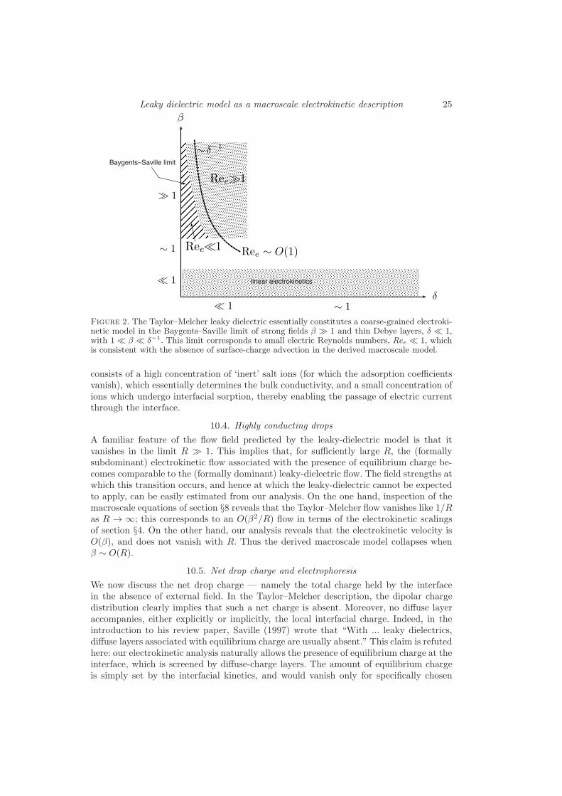
The linearity of the electrostatic problem, which enables analytic solution of the macroscalemodel, follows from the absence of surface convection of charge. In our macroscale model,this absence automatically follows from the Baygents–Saville limit (1.1). Indeed, for theeffective O(δβ2) surface current associated with the leading O(β2) flow to enter the ionconservation equations (4.26) at the O(β) leading-order, β must be O(δ−1). Such largevalues of the applied field do not satisfy the restriction (5.2).In fact, the surface current associated with the leading O(β2) flow is asymptotically

smaller than O(δβ2). Indeed, as the O(β2) tangential velocity is transversely uniform(see (6.16)), the O(δβ2) surface current is simply provided by its product with the ap-parent O(1) Debye-layer charge; the latter, however, vanishes by screening: see (6.32). Itmay therefore appear that the leading-order surface current is due to the leading O(δβ)apparent charge, and is accordingly O(δ2β3). Note however that another source for asurface current is the O(β) electro-osmotic flow, which we did not bother to calculate.As this flow is transversely nonuniform, it results through advection of the O(1) ionicdensities in an O(δβ) surface current. The Baygents–Saville restriction (5.2) does not de-termine which of these two effects dominates. The corrections implied by these currentsto the charge-conservation condition (7.5), where the Ohmic currents are O(β), are ofrelative orders (δβ)2 and δ, respectively.In the electrohydrodynamic literature, the neglect of charge convection is convention-

ally associated with the assumption of small electric Reynolds number (see Melcher &Taylor 1969). Consider indeed the typical dimensional magnitude of the respective chargeconduction and convection terms in a surface-charge balance (e.g. Eq. Il in Melcher &


Taylor (1969)). The former is of order σ∗E∗, σ∗ being a typical conductivity, while thelatter, represented by a surface-divergence term, is of order Λ∗v∗/a∗, where Λ∗ is the ap-parent surface-charge density; in the leaky dielectric description, that density is of orderǫ∗E∗. It follows that the ratio of charge convection to conduction is of order ǫ∗v∗/σ∗a∗.This is the electric Reynolds number Ree.Following our derivation of the electrohydrodynamic Taylor–Melcher model as a coarse-

grained description, this number is easily estimated. Consider the simple case of equaldiffusivities D±

∗ = D∗, where α± are identical, = α say (see (4.4)). The bulk conductivity

σ∗ is then given by 2ze∗C∗D∗/ϕ∗, see (7.21). Using the leaky dielectric velocity scaleǫ∗a∗E

2∗/µ∗ we readily find using definitions (4.1), (4.4), (4.6) and (4.35) that

Ree = αδ2β2. (10.1)

Since α is typically O(1) (see (4.4) et seq.), the electric Reynolds number is asymptoticallysmall in the Baygents–Saville limit (1.1) underlying our electrokinetic description: seefigure 2.In the classical paper of Melcher & Taylor (1969), charge convection is presented in

the electrohydrodynamic model (see their Table I). It is then neglected throughout whenperforming steady analyses of specific configurations — in particular, in the analysis ofthe flow about a leaky dielectric drop. This neglect is introduced as an additional as-sumption. As Melcher & Taylor (1969) had no underlying electrokinetic model to providethe magnitude of the bulk conductivity, they could not have obtained the estimate (10.1).Note that the parts of the analysis of Melcher & Taylor (1969) which deal with insta-

bilities and fluid motion driven by alternating currents allow for finite electric Reynoldsnumber. Moreover, charge convection was incorporated in several electrohydrodynamicmodels (see Xu & Homsy 2006; Feng & Scott 1996; Salipante & Vlahovska 2010) in an at-tempt to improve upon Taylor’s initial analysis. In view of estimate (10.1), these studiesfall outside the Baygents and Saville regime, and hence their electrokinetic interpretationremains unclear.

10.3. The conductivity ratio: a material property?

The macroscale equations depend upon the permittivity ratio S, the viscosity ratio M ,and the conductivity ratio R, just as in the model outlined by Melcher & Taylor (1969).Melcher & Taylor (1969) consider these parameters as given material ratios. In our schemethere is however a conceptual difference between the permittivity and viscosity ratios SandM and the conductivity ratio R: while the former two represent (ratios between) truematerial properties (and actually appear in the microscope formulation), the latter is aderivedmacroscale quantity, which does not appear in the original formulation. In view ofexpression (8.12), moreover, R depends upon the adsorption coefficients (K±, K±) (nor-malised by 2/κ∗), and accordingly cannot be considered a material property. Puttingit differently, while the conductivity of the suspending liquid can be conceptually mea-sured in an experiment, independently of the drop, the same does not hold for the dropconductivity.This difference with the Taylor–Melcher model should be viewed with caution, however,

given our simplistic modelling of charge transfer across the interface and our simplifyingassumption of a strong binary electrolyte. A more realistic description of ionic transportwould incorporate bulk reactions (see e.g. Saville 1997) and allow only some of the ionicspecies to pass through the interface. Within the framework of such a general model, onecan envisage two scenarios where the drop-phase conductivity is effectively a propertyof the drop, unaffected by the passage of currents. The first is realized in the limit offast reactions, while the second occurs when the ionic composition in the two liquids


β

δ

≪ 1

∼ 1

≫ 1

∼ 1≪ 1

linear electrokinetics

∼δ−1

Baygents–Saville limit

Ree≪1

Ree≫1

Ree ∼ O(1)

Figure 2. The Taylor–Melcher leaky dielectric essentially constitutes a coarse-grained electroki-netic model in the Baygents–Saville limit of strong fields β ≫ 1 and thin Debye layers, δ ≪ 1,with 1 ≪ β ≪ δ−1. This limit corresponds to small electric Reynolds numbers, Ree ≪ 1, whichis consistent with the absence of surface-charge advection in the derived macroscale model.

consists of a high concentration of ‘inert’ salt ions (for which the adsorption coefficientsvanish), which essentially determines the bulk conductivity, and a small concentration ofions which undergo interfacial sorption, thereby enabling the passage of electric currentthrough the interface.

10.4. Highly conducting drops

A familiar feature of the flow field predicted by the leaky-dielectric model is that itvanishes in the limit R ≫ 1. This implies that, for sufficiently large R, the (formallysubdominant) electrokinetic flow associated with the presence of equilibrium charge be-comes comparable to the (formally dominant) leaky-dielectric flow. The field strengths atwhich this transition occurs, and hence at which the leaky-dielectric cannot be expectedto apply, can be easily estimated from our analysis. On the one hand, inspection of themacroscale equations of section §8 reveals that the Taylor–Melcher flow vanishes like 1/Ras R → ∞; this corresponds to an O(β2/R) flow in terms of the electrokinetic scalingsof section §4. On the other hand, our analysis reveals that the electrokinetic velocity isO(β), and does not vanish with R. Thus the derived macroscale model collapses whenβ ∼ O(R).

10.5. Net drop charge and electrophoresis

We now discuss the net drop charge — namely the total charge held by the interfacein the absence of external field. In the Taylor–Melcher description, the dipolar chargedistribution clearly implies that such a net charge is absent. Moreover, no diffuse layeraccompanies, either explicitly or implicitly, the local interfacial charge. Indeed, in theintroduction to his review paper, Saville (1997) wrote that “With ... leaky dielectrics,diffuse layers associated with equilibrium charge are usually absent.” This claim is refutedhere: our electrokinetic analysis naturally allows the presence of equilibrium charge at theinterface, which is screened by diffuse-charge layers. The amount of equilibrium chargeis simply set by the interfacial kinetics, and would vanish only for specifically chosen


combinations of the respective coefficients. In the physicochemical model (4.32), zerodrop charge is realized for K+ = K− = K+ = K− and S = 1 — see (6.27) and(6.29). In the general case, then, the charge on the genuine interface is nonzero. In fact,the presence of nonzero interfacial charge is actually necessary for the validity of ourasymptotic scheme, which hinges upon the induced charge being a small perturbation.Our analysis reveals that, remarkably, the electrophoretic motion engendered by the

net drop charge constitutes an asymptotic correction to the Taylor–Melcher flow, itselfanimated by a perturbation to that equilibrium charge. The appearance of electrophore-sis at a higher order might be consistent with existing experiments, where the dropindeed tends to move under the electric field. (Such motion was considered as an in-evitable inconvenience that interferes with the convenient observation and measurementof electrohydrodynamic drop deformation, see Taylor 1966 and Vizika & Saville 1992.)Our unified approach provides the means for understating this inevitable motion, which

apparently goes hand in hand with the Taylor–Melcher flow. The calculation of drop elec-trophoresis in our scheme requires continuing the asymptotic analysis towards derivinga higher-order macroscale model. Such an analysis reveals that drop electrophoresis isanimated by both shear and a two-sided electro-osmotic slip mechanism. While the latteris already implied in our analysis (see (7.13)), the calculation of the shear contributionentails a complicated calculation, including the resolution of the two diffusive boundarylayers. In the limit of a highly-viscous drop, one can show that the shear contributionbecomes trivial. The drop thus migrates according to a Smoluchowski-type formula, withthe zeta potential appearing therein being that of the external Debye layer. Interest-ingly then, the equilibrium charge in that case cannot be straightforwardly inferred fromelectrophoretic measurements.The compatibility of nonzero net charge with the absence of electrophoresis at leading

order is clearly a manifestation of the delicate limit process (1.1), representing the strongfields characterising Taylor–Melcher flows. This compatibility casts doubts regarding theapplicability of the scheme developed by Zholkovskij, Masliyah & Czarnecki (2002). Inthat paper, which proposes a different approach to model the transition from electrokinet-ics to electrohydrodynamics, the Taylor–Melcher description is developed for an arbitraryDebye length. In sharp contrast to Baygents & Saville (1989), this is accomplished viaa weak-field approximation. Putting aside the validity of such an approximation in de-scribing Taylor–Melcher flows, it appears that the main shortcoming in the analysis ofZholkovskij et al. (2002) is the necessity of assuming zero net charge; as the authorsexplain, this corresponds to artificially specifying appropriate ratios of the kinetic pa-rameters. Similarly, the recent stability analysis of Gambhire & Thaokar (2014) alsomakes use of an effective weak-field linearisation. In that paper the authors avoid thearbitrariness in the kinetic approach of Zholkovskij et al. (2002) by focusing upon inertsolute which does not adsorb to the genuine interface. While this gives rise to a consistentphysical model, the absence of ionic transport through the interface renders it insufficientwhen attempting to describe the electrokinetics underlying the leaky–dielectric model.

This research was supported by the Israel Science Foundation (grant no. 184/12).

Appendix A. Salt uniformity

Since the flow fields u−2 and u−2 are steady in the co-moving reference frame weemploy, equations (5.11) state that c0 and c0 are constant along the respective streamlinesof these fields. For open streamlines which originate at infinity such constancy wouldreadily provide the values of c0 using its far-field distribution (given here by (4.33a)),


thus leading to the uniform salt distribution (5.12). We now show that c0 is uniform aswell. We follow a method devised by Batchelor (1956) in the different context of vorticitydynamics at large-Reynolds-number flow.

The proof makes use of (i) the fact that the streamlines of the steady flow u−2 arebounded by the drop boundary and are accordingly all closed; and (ii) the axial symmetryof the leading order flow, which is justified a posteriori. We employ the integral form ofthe salt balance equation (4.21),

∮

S

dA n ·

{

j +

(

α+ + α−

2c+

α+ − α−

2q

)

u

}

= 0, (A 1)

wherein S is the boundary of an arbitrary domain lying entirely within the drop phaseand n is a unit vector normal to S. Specifically, consider a streamline of u and imaginethe torus-like surface S formed by rotating it about the symmetry axis. As n · u = 0 onthat surface, (A 1) reads

∮

S

dA n · j = 0. (A 2)

We now consider the limit δ → 0, where u → u−2. Because of axial symmetry, u−2 isderived from a Stokes streamfunction, say ψ−2. Since c0 is constant on the streamlines ofu−2, it follows that it is a function of ψ−2. As δ → 0, then, S is given by a constant-ψ−2

surface, while j → j0:∮

ψ−2=const

dA n · j0 = 0. (A 3)

Use of (5.8b) then yields:∮

ψ−2=const

dA∂c0∂n

= 0. (A 4)

At this point we conceptually construct a system of (ξ, η) orthogonal coordinates inthe meridian plain with ξ = ψ−2 and the level curves of η orthogonal to those of ψ−2.The fluid domain is therefore described via a curvilinear (ξ, η,) coordinate system, being the azimuthal angle already defined in §4.3. In these coordinates, c0 is a functionof ξ alone, independent of η and . Moreover, since the integration domain in (4.3) is aconsent-ξ surface, it is evident (tacitly choosing n pointing in the direction of increasingψ−2) that on that surface ∂c0/∂n = (1/hξ)dc0/dξ, where hξ is the metric coefficientassociated with the curvilinear coordinate ξ (in general a function of both ξ and η).Since dc0/dξ, a function of ξ, is constant on the integration surface, it may be takenoutside the integral. Equation (A 4) becomes

dc0dξ

∮

ξ=const

dA

hξ= 0. (A 5)

Since hξ > 0, this implies that

dc0dξ

= 0. (A 6)

Since the integration domain is an arbitrary stream surface, (A 6) holds for all values ofξ(= ψ−2). It follows that c0 is independent of ψ−2 and hence uniform.


Appendix B. Normal-stress jump

Expressed in terms of the Debye-layer variables, the microscale normal-stress jumpacross the interface is provided by the expression:

−P−P+2

(

∂U

∂Z−M−1∂U

∂Z

)

δ−1+1

2δ2

[

(

∂Φ

∂Z

)2

− S−1

(

∂Φ

∂Z

)2]

−1

2

(

1− S−1)

(

∂Φ

∂θ

)2

.

(B 1)In what follows we express this quantity in terms of the macroscale variables.Inspection of the radial momentum balance in the Debye layer suggests the pressure

expansion

P = δ−2P−2,0 + δ−1βP−1,−1 + δ−1P−1,0 + β2P0,−2 + · · · . (B 2)

The radial momentum balance at leading O(δ−3) reads

∂P−2,0

∂Z=∂2Φ0,0

∂Z2

∂Φ0,0

∂Z. (B 3)

Since the bulk pressure is only O(β2), and given the exponential decay of Φ0,0 as Z → ∞,integration of (B 3) simply yields

P−2,0 =1

2

(

∂Φ0,0

∂Z

)2

. (B 4)

A similar expression is obtained for P−2,0:

P−2,0 =1

2S

(

∂Φ0,0

∂Z

)2

. (B 5)

Substitution into (B 1) thus reveals that the stress jump at O(δ−2) trivially vanishes.Continuing on, the radial momentum balance at O(δ−2β) reads

∂P−1,−1

∂Z=∂2Φ0,0

∂Z2

∂Φ1,−1

∂Z+∂2Φ1,−1

∂Z2

∂Φ0,0

∂Z. (B 6)

Noting again the rapid decay of Φ0,0 and the absence of O(δ−1β) bulk pressure, we obtain

P−1,−1 =∂Φ0,0

∂Z

∂Φ1,−1

∂Z, (B 7)

with a similar expression in the drop phase,

P−1,−1 = S−1 ∂Φ0,0

∂Z

∂Φ1,−1

∂Z. (B 8)

Substitution into (B 1) reveals that the stress jump at O(δ−1β) vanishes as well.Returning to the radial momentum balance, this time at O(δ−2), we find

∂P−1,0

∂Z= 2

(

∂Φ0,0

∂Z

)2

, (B 9)

representing the effect of drop curvature. Integrating with respect to Z from 0 to ∞,where P−1,0 must vanish due to the absence of O(δ−1) pressure term in the bulk, wefind that P−1,0(Z = 0) is provided by a quadrature of ∂Φ0,0/∂Z. Since this derivativein independent of θ (see §6.3), so must be P−1,0(Z = 0). A similar argument applies forP−1,0(Z = 0). Since a uniform normal-stress jump does not contribute to a deformationfrom sphericity, it may be disregarded.


Finally, the radial momentum balance at O(δ−1β2) reads

∂P0,−2

∂Z=∂2U1,−2

∂Z2+∂2Φ1,−1

∂Z2

∂Φ1,−1

∂Z. (B 10)

Integrating, and using the matching conditions

P0,−2 → p0,−2,∂U1,−2

∂Z→

∂u0,−2

∂r,

∂Φ1,−1

∂Z→

∂ϕ0,−1

∂r, (B 11)

we find that

P0,−2 −∂U1,−2

∂Z= p0,−2 −

∂u0,−2

∂r−

1

2

(

∂ϕ0,−1

∂r

)2

+1

2

(

∂Φ1,−1

∂Z

)2

. (B 12)

Repeating the calculation for the drop-phase pressure at this order, we find that the firstnon-vanishing (and non-constant) normal-pressure jump is O(β2), namely

β2

{

−p0,−2 + p0,−2 + 2

(

∂u0,−2

∂r−M−1 ∂u0,−2

∂r

)

+1

2

[

(

∂ϕ0,−1

∂r

)2

− S−1

(

∂ϕ0,−1

∂r

)2]

−1

2

(

1− S−1)

(

∂ϕ0,−1

∂θ

)2}

. (B 13)

This however is the expression which would be provided using the effective macroscalemodel.

REFERENCES

Acrivos, A. & Goddard, J. D. 1965 Asymptotic expansions for laminar forced-convectionheat and mass transfer. Part 1. Low speed flows. J. Fluid Mech. 23 (02), 273–291.

Anderson, J. L. 1989 Colloid transport by interfacial forces. Annu. Rev. Fluid Mech. 30,139–165.

Batchelor, G. 1956 On steady laminar flow with closed streamlines at large reynolds number.J. Fluid Mech 1 (2), 177–190.

Baygents, J. C. & Saville, D. A. 1989 The circulation produced in a drop by an electricfield: a high field strength electrokinetic model. In Drops & Bubbles, Third InternationalColloquium, Monterey 1988 (ed. T. Wang), vol. 7, pp. 7–17. AIP Conference Proceedings,New York: Am. Inst. Physics.

Baygents, J. C. & Saville, D. A. 1991 Electrophoresis of drops and bubbles. J. Chem. Soc.,Faraday Trans. 87 (12), 1883–1898.

Ben, Y., Demekhin, E. A. & Chang, H.-C. 2004 Nonlinear electrokinetics and “superfast”electrophoresis. J. Colloid Interface Sci. 276, 483–497.

Chu, K. T. & Bazant, M. Z. 2006 Nonlinear electrochemical relaxation around conductors.Phys. Rev. E 74 (1), 011501.

Craster, R. V. & Matar, O. K. 2005 Electrically induced pattern formation in thin leakydielectric films. Phys. Fluids 17 (3), 032104.

Derjaguin, B. V. & Dukhin, S. S. 1974 Nonequilibrium double layer and electrokinetic phe-nomena. In Electrokinetic phenomena (ed. E. Matijevic), Surface and Colloid Science,vol. 7, pp. 273–336. New York: John Wiley.

Feng, J. Q. 1999 Electrohydrodynamic behaviour of a drop subjected to a steady uniformelectric field at finite electric reynolds number. Proc. Roy. Soc. London. A 455 (1986),2245.

Feng, J. Q. & Scott, T. C. 1996 A computational analysis of electrohydrodynamics of a leakydielectric drop in an electric field. J. Fluid Mech. 311, 289–326.

Gambhire, P. & Thaokar, R. 2014 Electrokinetic model for electric-field-induced interfacialinstabilities. Phys. Rev. E 89 (3), 032409.

Leal, L. G. 2007 Advanced Transport Phenomena: Fluid Mechanics and Convective TransportProcesses. New York: Cambridge University Press.


Mani, A. & Bazant, M. Z. 2011 Deionization shocks in microstructures. Phys. Rev. E 84 (6),061504.

Melcher, J. R. & Taylor, G. I. 1969 Electrohydrodynamics: a review of the role of interfacialshear stresses. Ann. Rev. Fluid Mech. 1 (1), 111–146.

Monroe, C. W., Daikhin, L. I., Urbakh, M. & Kornyshev, A. A. 2006 Electrowetting withelectrolytes. Phys. Rev. Lett. 97 (13), 136102.

Morrison, F. A. 1970 Electrophoresis of a particle of arbitrary shape. J. Colloid Interface Sci.34, 210–214.

O’Brien, R. W. 1983 The solution of the electrokinetic equations for colloidal particles withthin double layers. J. Colloid Interface Sci. 92 (1), 204–216.

Ohshima, H., Healy, T. W. & White, L. R. 1984 Electrokinetic phenomena in a dilutesuspension of charged mercury drops. J. Chem. Soc., Faraday Trans. 2 80 (12), 1643–1667.

Rivette, N. J. & Baygents, J. C. 1996 A note on the electrostatic force and torque actingon an isolated body in an electric field. Chem. Engng Sci. 51 (23), 5205–5211.

Salipante, P. F. & Vlahovska, P. M. 2010 Electrohydrodynamics of drops in strong uniformdc electric fields. Phys. Fluids 22, 112110.

Salipante, P. F. & Vlahovska, P. M. 2014 Vesicle deformation in DC electric pulses. Softmatter 10 (19), 3386–3393.

Saville, D. A. 1977 Electrokinetic effects with small particles. Annu. Rev. Fluid Mech. 9,321–337.

Saville, D. A. 1997 Electrohydrodynamics: the Taylor–Melcher leaky dielectric model. Ann.Rev. Fluid Mech. 29 (1), 27–64.

Schnitzer, O., Frankel, I. & Yariv, E. 2013a Electrokinetic flows about conducting drops.J. Fluid Mech. 722, 394–423.

Schnitzer, O., Frankel, I. & Yariv, E. 2014 Electrophoresis of bubbles. J. Fluid Mech. 753,49–79.

Schnitzer, O. & Yariv, E. 2012a Macroscale description of electrokinetic flows at large zetapotentials: Nonlinear surface conduction. Phys. Rev. E 86, 021503.

Schnitzer, O. & Yariv, E. 2012b Strong-field electrophoresis. J. Fluid Mech. 701, 333–351.Schnitzer, O. & Yariv, E. 2013 Nonlinear electrokinetic flow about a polarized conducting

drop. Phys. Rev. E 87, 041002R.Schnitzer, O., Zeyde, R., Yavneh, I. & Yariv, E. 2013b Nonlinear electrophoresis of a

highly charged colloidal particle. Phys. Fluids 25, 052004.Taylor, G. 1966 Studies in electrohydrodynamics. I. The circulation produced in a drop by

electrical field. Proc. Roy. Soc. London A 291 (1425), 159–166.Torza, S., Cox, R. G. & Mason, S. G. 1971 Electrohydrodynamic deformation and burst of

liquid drop. Philos. Tr. R. Soc. S-A 269 (1198), 295–319.Vizika, O. & Saville, D. A. 1992 The electrohydrodynamic deformation of drops suspended

in liquids in steady and oscillatory electric fields. J. Fluid Mech. 239 (1), 1–21.Xu, X. & Homsy, G. M. 2006 The settling velocity and shape distortion of drops in a uniform

electric field. J. Fluid Mech. 564, 395–414.Yariv, E. 2009 An asymptotic derivation of the thin-Debye-layer limit for electrokinetic phe-

nomena. Chem. Engng Commun. 197, 3–17.Yariv, E. 2010 Migration of ion-exchange particles driven by a uniform electric field. J. Fluid

Mech. 655, 105–121.Yariv, E., Schnitzer, O. & Frankel, I. 2011 Streaming-potential phenomena in the thin-

Debye-layer limit. Part 1. General theory. J. Fluid Mech. 685, 306–334.Zholkovskij, E. K., Masliyah, J. H. & Czarnecki, J. 2002 An electrokinetic model of drop

deformation in an electric field. J. Fluid Mech. 472 (1), 1–27.

The Taylor–Melcher leaky dielectric model as a macroscale ...

Documents

Transcript of The Taylor–Melcher leaky dielectric model as a macroscale ...