This article appeared in a journal published by Elsevier. The attachedcopy is furnished to the author for internal non-commercial researchand education use, including for instruction at the authors institution

and sharing with colleagues.

Other uses, including reproduction and distribution, or selling orlicensing copies, or posting to personal, institutional or third party

websites are prohibited.

In most cases authors are permitted to post their version of thearticle (e.g. in Word or Tex form) to their personal website orinstitutional repository. Authors requiring further information

regarding Elsevier’s archiving and manuscript policies areencouraged to visit:

http://www.elsevier.com/copyright

Author's personal copy

Tidal and residual circulations in coupled restricted and leaky lagoons

Thomas Guyondet*, Vladimir G. Koutitonsky

Institut des Sciences de la Mer de Rimouski (ISMER), Universite du Quebec a Rimouski, 310 Allee des Ursulines, Rimouski, QC G5L 3A1, Canada

Received 18 July 2007; accepted 2 October 2007

Available online 30 October 2007

Abstract

Finite element numerical modelling based on field data is used to study the tidal and tidally induced residual circulation dynamics of a cou-pled ‘‘restricted’’ and ‘‘leaky’’ coastal lagoon system located in the Magdalen Islands, Gulf of Saint-Lawrence. Havre-aux-Maisons Lagoon(HML) is of a ‘‘restricted’’ nature with a neutral inlet in terms of tidal asymmetry. Grande-Entree Lagoon (GEL) is of a ‘‘leaky’’ naturewith a marked ebb dominance at the inlet due to direct interactions between the main astronomical tidal constituents. The imbalance causedby the different tidal filtering characteristics of both inlets combines with the internal morphological asymmetries of the system to producea residual throughflow from HML to GEL. The residual circulation is also characterized by strongest values at both inlets, very weak residualcurrents in HML deep basin and a dipole of residual eddies over the deeper areas of GEL. Further investigations including numerical tracerexperiments will be necessary to achieve a full understanding of the long term circulation of this lagoonal system.� 2007 Elsevier Ltd. All rights reserved.

Keywords: coastal lagoons; hydrodynamics; residual flow; inlet morphology; tidal asymmetry; Canada; Gulf of Saint-Lawrence; Magdalen Islands; 47�300N61�400W

1. Introduction

Lagoons are highly attractive places owing to their abun-dant natural and recreational resources, sheltered areas and/or beautiful landscapes. However, due to their narrow connec-tion to the open ocean, they are, among other coastal systems,the most sensitive to human disturbances. Their restricted con-nections to the open sea often reduce their ability to flushexogenous substances leading to poor water renewal, eutrophi-cation and other water quality problems. Hence, understandingwater circulation within lagoons and their exchanges with theopen sea becomes a prerequisite for sustainable managementof these systems.

Several studies have addressed the exchange and transportprocesses between lagoons and oceans (Longuet-Higgins, 1969;van de Kreeke, 1976; Dronkers and Zimmerman, 1982). Themethods used are either based on tidal asymmetry (Aubrey

and Speer, 1985; Fry and Aubrey, 1990; van Maren et al.,2004) or on residual flow determination (Longuet-Higgins,1969; Feng et al., 1986a,b; Tee and Lefaivre, 1990; Ridderink-hof and Loder, 1994; Loder et al., 1997; Janzen and Wong,1998; Wei et al., 2004), with the latter giving a detailed spatialrepresentation of transport processes. Residual circulation incoastal areas may be generated either by non-linear interac-tions between tidal constituents and topography and bathyme-try (tide-induced), wind stress, density gradients, fresh waterinflows or external water level gradients for multiple inlet sys-tems (Uncles, 1982; Feng et al., 1986b; Smith, 1990; LeBlond,1991; Prandle, 1991; Aubrey et al., 1993). Given the numberof processes involved, recent studies have ultimately reliedon numerical models. Particular attention must be given toforcing functions in the coastal area as they set the spatialand temporal variability of the system. In the absence of freshwater input, tides and meteorological conditions are usually themost influencing forcings. Even though meteorological forcingis important at times (Smith, 1990), tides will remain the dom-inant periodic forcing in most cases. Finally, inlet morphology,topography and bathymetry play a major role in the dynamics

* Corresponding author.

E-mail addresses: thomas_guyondet@uqar.qc.ca (T. Guyondet), vgk@

uqar.qc.ca (V.G. Koutitonsky).

0272-7714/$ - see front matter � 2007 Elsevier Ltd. All rights reserved.

doi:10.1016/j.ecss.2007.10.009

Available online at www.sciencedirect.com

Estuarine, Coastal and Shelf Science 77 (2008) 396e408www.elsevier.com/locate/ecss

Author's personal copy

of coastal lagoons and other semi-enclosed coastal systems(Keulegan, 1967; Zimmerman, 1981; DiLorenzo, 1988; vande Kreeke, 1988; Shetye and Gouveia, 1992; Aubrey et al.,1993; Fortunato and Oliveira, 2005). Therefore, the knowledgeof external forcing alone is not sufficient as the response ofeach coastal lagoon depends on its tidal inlet geomorphologyand, as such, is unique. In fact, coastal lagoons have beensubdivided according to their tidal and morphological chara-teristics into ‘‘choked’’, ‘‘restricted’’ and ‘‘leaky’’ systems(Kjerfve, 1986). This classification confirms the tight link be-tween the inlet characteristics and the ability of the lagoon toexchange water with the open sea (Kjerfve and Knoppers,1991).

The objective of the present work is to investigate the tidaldynamics and the tide-induced residual circulation of a coupledtwo-lagoon system and reach a better understanding of howtheir inlet characteristics affect the transport and exchangeprocesses between them and the open sea. A numerical modelis set up to accurately represent the dynamics of this systemunder the influence of natural forcings. The finite elementmethod was chosen for its ability to accurately representcomplex coastlines (Legrand et al., 2006). The tidal residualsare known to be highly influenced by the topography of thesystem. Hence, an unstructured grid that allows an additional

refinement close to the shore helps to avoid unrealistic resid-uals in coastal areas (Jones and Davies, 2007). This numericalstudy of residual circulation and the development of the 3Dhydrodynamic model is a first step towards a more comprehen-sive study of the long-term circulation of this lagoonal systemand the three-dimensional ecosystem dynamics of one of thelagoons.

2. Material and methods

2.1. Study area

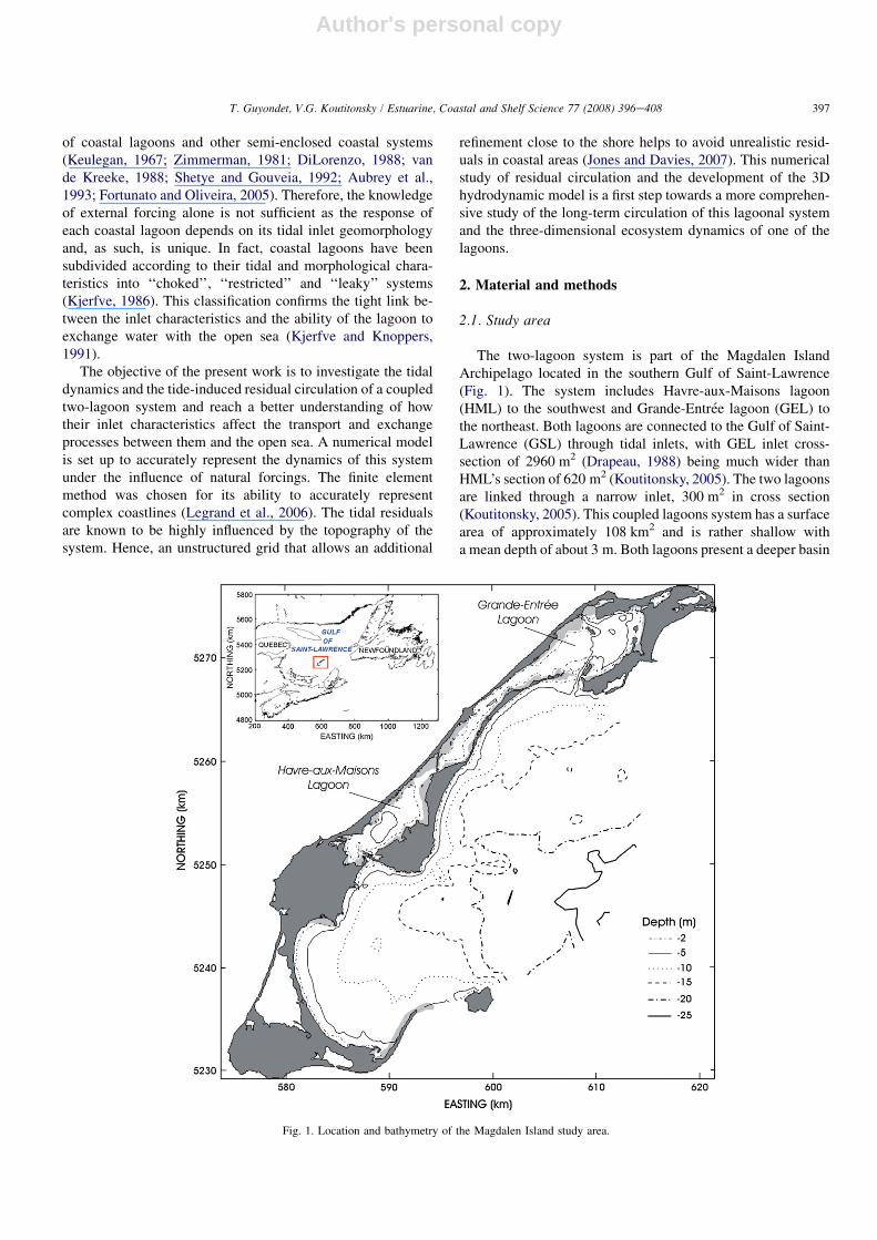
The two-lagoon system is part of the Magdalen IslandArchipelago located in the southern Gulf of Saint-Lawrence(Fig. 1). The system includes Havre-aux-Maisons lagoon(HML) to the southwest and Grande-Entree lagoon (GEL) tothe northeast. Both lagoons are connected to the Gulf of Saint-Lawrence (GSL) through tidal inlets, with GEL inlet cross-section of 2960 m2 (Drapeau, 1988) being much wider thanHML’s section of 620 m2 (Koutitonsky, 2005). The two lagoonsare linked through a narrow inlet, 300 m2 in cross section(Koutitonsky, 2005). This coupled lagoons system has a surfacearea of approximately 108 km2 and is rather shallow witha mean depth of about 3 m. Both lagoons present a deeper basin

Fig. 1. Location and bathymetry of the Magdalen Island study area.

397T. Guyondet, V.G. Koutitonsky / Estuarine, Coastal and Shelf Science 77 (2008) 396e408

Author's personal copy

on their eastern side where depths vary between 5 and 6 m. Acharacteristic for GEL is the presence of a dredged 8 m deepnavigation channel going from the entrance up to the northernshore (Fig. 1).

This coupled system is mainly forced by tides and meteoro-logical processes as there is no river discharge into the lagoons.Tides on the shallow (ca. 50 m) Magdalenian bank surroundingthe islands are of small amplitude (0.5 m during spring tides)and of mixed but mainly semi-diurnal type (Koutitonskyet al., 2002). Stations shown in Fig. 2 were used in summer2001 (MayeJuly) to monitor water levels and/or currents atdifferent points of interest in the system (tide gauges and cur-rent meters moored at 1 m above the bottom). Hourly timeseries of wind speed and direction and atmospheric pressurewere recorded at station M (Fig. 2) and were considered tobe constant over the whole model domain. Water levels re-corded at external stations L10 and L11 served as boundaryconditions for the model simulations while stations inside thelagoons were used for model calibrations (see next section).

Regional atmospheric forcings are known to affect low fre-quency water level fluctuations through an inverse barometereffect of the atmospheric pressure and a non-local wind setup/down effect at the scale of the GSL (Koutitonsky et al.,2002). Local winds are predominantly blowing from the west-ern sector and calm conditions are scarce (Drapeau, 1988).Moreover a predominant orientation of the wind along thelongitudinal axis of the lagoonal system has been noticed(Koutitonsky et al., 2002). Another characteristic of this sys-tem is the presence of an ice cover from January to mid-Aprilin average conditions (Drapeau, 1988). The present work fo-cuses only on the deterministic effects of tidal forcing aloneduring the ice-free season.

In this context, both lagoon-inlet systems set the way exter-nal forcings are transmitted to the inner parts of the system(DiLorenzo, 1988). GEL and HML inlets may be broadlycharacterized using the repletion coefficient (K ) defined as(Keulegan, 1967; van de Kreeke, 1988; Kjerfve and Knoppers,1991):

K ¼ T

2pa0

AC

AB

ffiffiffiffiffiffiffiffiffiffiffiffiffiffiffiffiffiffiffiffiffiffiffiffiffiffiffiffiffiffiffiffiffiffiffiffiffiffiffiffiffiffi2gRa0

ðaþ bþ gÞRþ 2FLC

sð1Þ

with the semi-diurnal tidal period T ¼ 12.42 h, the semi-diurnal tidal amplitude a0 ¼ 0.2 m, the inlet cross-sectionsAC mentioned above, the lagoon surface areas AB ¼ 34 and74 km2 for HML and GEL respectively, the hydraulic radiiat the entrance R ¼ 4.1 and 3.8 m, respectively, and the accel-eration due to gravity g. As the friction factors F (0.002 to0.006) were not known a priori for HML and GEL inletsand as the repletion coefficient only varies of 0.3 (HML)and 0.5 (GEL) over the whole range of F values, the medianvalue of 0.004 was used for both inlets. The length of the inletsLC was set to 700 and 2000 m for HML and GEL respectively.The parameter a accounting for the velocity distribution overthe inlet cross-section was set to 0.3 for GEL where the flow isconcentrated by the navigation channel over a small part of thecross-section and to 0.2 for HML which exhibits a narrowerinlet with uniform dephts. The coefficient b corresponds tothe fraction of kinetic energy dissipated in the transition be-tween the entrance and the inlet channel. Both inlets presentrelatively smooth transitions due to the slowly convergentcoastlines for HML and due to the navigation channel extend-ing offshore for GEL. Hence, the same value b ¼ 0.3 was usedfor both. Finally, g represents the fraction of remaining kineticenergy lost at the lagoon side of the inlet. In the absence of anymajor channel and due to the rapidly divergent coastlinesHML’s inlet presents a much more abrupt transition thanGEL’s leading to a larger dissipation of kinetic energy. Toreflect this g was given a value of 0.7 for HML and 0.3 forGEL (van de Kreeke, 1988). According to the classificationintroduced by Kjerfve (1986) and values of K ¼ 1.2 andK ¼ 0.7 for GEL and HML respectively this system is a cou-pled ‘‘leaky’’ (GEL) and ‘‘restricted’’ (HML) lagoonal system.

It is now possible to assess the conditions set inside bothlagoons by these dynamically different inlets and examinehow these conditions interact through the tight connexion be-tween HML and GEL to have a complete picture of the systemcirculation behaviour.

2.2. Model description

2.2.1. General characteristicsThe model used for the present work is RMA-10 (King,

1982). It is a three-dimensional (3D) finite element hydrody-namic model developped for coastal and estuarine systems.It uses the NewtoneRaphson iterative approach with theGalerkin weighted residuals to solve a 3D set of non linearequations. These basic equations are the Reynolds form of

Fig. 2. Location of the summer 2001 sampling stations (L: tidal gauge; C: cur-

rent meter; M: meteorological station) and calculation grid of the numerical

model RMA-10 with its two open boundaries (OBD1 and OBD2).

398 T. Guyondet, V.G. Koutitonsky / Estuarine, Coastal and Shelf Science 77 (2008) 396e408

Author's personal copy

the NaviereStokes equations for motion, the continuity equa-tion, a convection-diffusion equation for transport of heat and/or salinity and the equation of state for density (see AppendixA). The momentum equation in the vertical direction is simpli-fied using the hydrostatic assumption. In the vertical, themodel uses a modified sigma transformation that preservesthe original bottom profile or a Z-level coordinate (King,1985). Another feature of RMA-10 is the possibility to mixdifferent levels of spatial representation in the same applica-tion. For instance, the model domain may be represented byareas where 3D equations are solved, next to shallower areaswhere the depth-averaged 2D equations are solved. This im-proves the calculation cost as compared to a full 3D applica-tion (King, 1985). RMA-10 also offers different options forturbulence closure methods. In this study, the Smagorinskyclosure scheme (Smagorinsky, 1963) was used in the horizon-tal. In the vertical, the original RMA-10 scheme was used. Inthis scheme, the vertical eddy viscosity coefficients are onlyvarying with depth and are given a quadratic distributionover the water column with a mid-depth maximum value de-termined during the calibration process. A constant verticaleddy viscosity wich is a too rough parametrization is improvedhere by this parabolic profile. As shown by Lee and Davies(1999) such a vertical eddy viscosity may be sufficient to rep-resent the overall tidal dynamics of a coastal system but a crit-ical point in assessing the quality of model results lies in thecomparison of observed and simulated near-bed currents.Despite near-bed current data are scarce, this comparison ispresented in the calibration section (Section 3.1) for twocritical areas of the system, namely HML’s and GEL’s inlets.Finally, RMA-10 uses a modified semi-implicit CrankeNicolson time stepping scheme for unsteady flows whichallows the use of rather long time steps, reducing the calcula-tion time (King, 1993).

2.2.2. Application to the Magdalen Island systemThe RMA-10 model was employed for the HML-GEL la-

goonal system based on data collected in summer 2001. Thehorizontal finite element grid structure used for this study isshown on Fig. 2. Considering subsequent ecosystem modellingrequirements and CTD profiles showing only slight thermalstratification during calm summer conditions (Booth, 1994),the vertical structure of the 3D model consisted of two verticallayers (3 nodes) of equal thickness. Most of the elements areof a quadrangular shape and a few triangles complete thegrid in less regular regions. A poor representation of the coast-line may lead to the generation of unrealistic tidal residuals(Jones and Davies, 2007). The refinement strategy hence con-sisted in maximizing the grid resolution in shallow nearshoreareas. The grid was also refined along the navigation channelinside GEL to better represent this deep and narrow feature ex-pected to play an important role in the lagoon hydrodynamics.The elements have typical side lengths varying between 80 min the most refined areas inside the lagoons to 2000 m for thecoarser part in the GSL. The 3D grid is composed of 6587 qua-dratic elements for a total of 19,333 nodes. The model domainhas two open boundaries (OBD1 and OBD2) where water

levels have been specified. The positions of OBD1 andOBD2 were set as far as possible from the actual entrancesof the lagoonal system in order not to bias the dynamics ofthe inlet areas. Water levels at station 11 were imposed alongOBD1, while a linear interpolation between water levels atstations 11 and 10 was imposed along OBD2. Finally, atmo-spheric pressure and wind friction were imposed on the freesurface during the calbration process. Given the lack of riverdischarge and the observed small density gradients either inhorizontal or vertical direction during the summer period, allsimulations were done with a constant density distribution(barotropic conditions). A time step Dt ¼ 360 s was used forall simulations leading to a maximum CFL number of approx-imately 4.5 in the most refined areas of the grid. All dataneeded for initial conditions, boundary conditions and forcingswere collected simultaneously during the 2001 field samplingmentioned above.

Two types of simulations, both covering the same 31-day-long period (from May 25 to June 25, 2001), were carriedout. These simulations differ by the set of forcings used:

(a) ‘‘REAL’’ simulation: The model is forced by observed wa-ter level fluctuations at the open boundaries and meteoro-logical forcing at the surface. This represents conditionsclosest to reality and this simulation was used for calibra-tion purposes only.

(b) ‘‘TIDAL’’ simulation: the model is forced by pure tidaloscillations at the open boundaries (obtained from the har-monic analysis of observed water level fluctuations; Fore-man, 1977). This simulation was used for the study of thetidally induced residual circulation described in the nextsections.

2.3. Residual flows and water levels

Model results from the ‘‘Tidal’’ simulation were analyzedfor residuals using the harmonic analysis of water levels (Z0)and currents (U0, V0) at each node of the grid. This simulationbeing forced by tidal oscillations only the residuals obtainedare internally generated by the dynamical behaviour of thelagoonal system.

A two day spin up period was allowed for the model tostabilize, then the residual flows and water levels in HMLand GEL were evaluated over the period corresponding tothe last 29 diurnal cycles of the simulation.

3. Results

3.1. Model calibration

Results of the ‘‘Real’’ simulation were used for tuning themodel. The calibration was based on two parameters, thebottom friction scaled by a unique Manning coefficient (n)over the whole area and the maximum value of the verticaleddy coefficient (3Z). The process relied on the comparisonof observed and simulated water levels (stations 1, 3, 4, 5, 6,7 and 9) and bottom currents (stations 2 and 8). The best

399T. Guyondet, V.G. Koutitonsky / Estuarine, Coastal and Shelf Science 77 (2008) 396e408

Author's personal copy

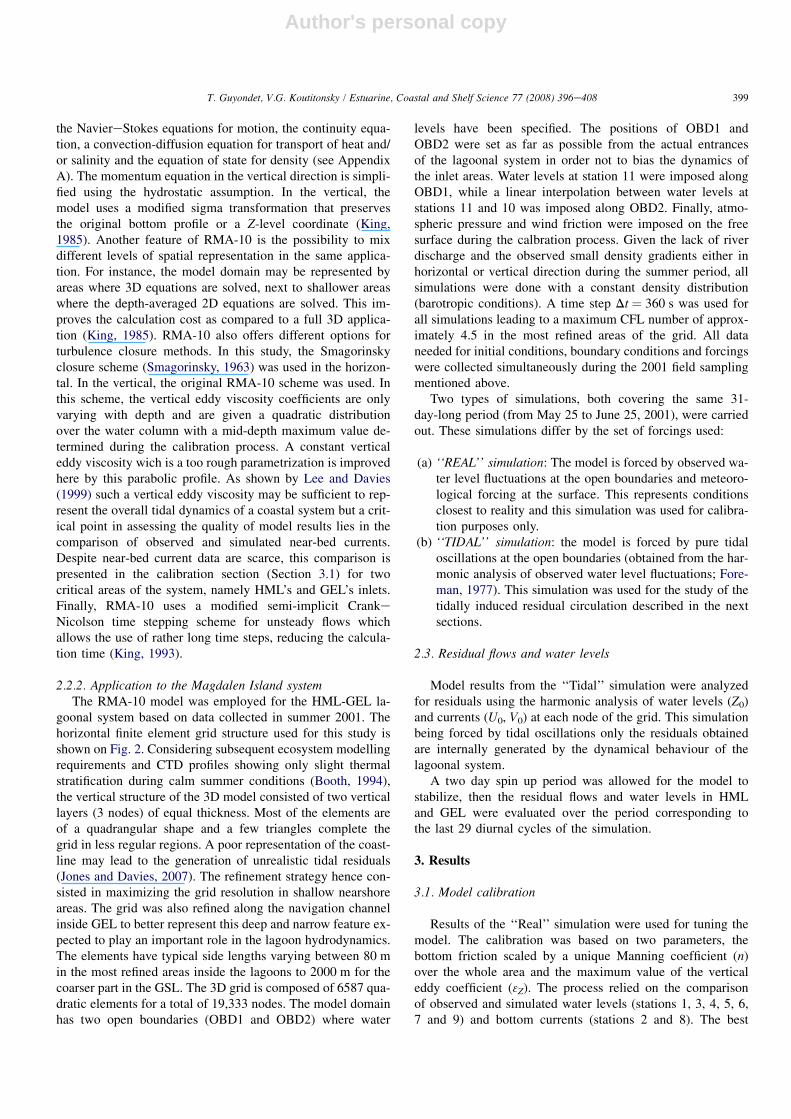
results were obtained for n ¼ 0.031 and 3Z ¼ 1 Pa s. Fig. 3a,bshows the comparison between observed and simulated waterlevels inside each lagoon at stations 4 and 6 respectively. Bothphase and amplitude of the water level fluctuations are well re-produced by the model. Harmonic analysis of observed andsimulated water levels was also made for all sampling stationslocated inside the model domain. Results for the main tidalcomponents O1, K1, M2 and S2 are presented in Table 1. Ex-cept for station 5 located at the junction of HML and GELwhere the phase of the semi-diurnal constituants is slightlyoff, model results are in close agreement with observations.This indicates that the tidal part of the water level fluctuationsis well described by the model in most of the system. TheMO3 constituent is also included in Table 1 to representshallow water waves generated by non-linear processes insidethe system. Model results are in fairly good agreement withobserved values of amplitude and phase of this compoundtide. This indicates a rather good representation of non-linearprocesses by the model. Stations 5 and 7 present the greatestdeviation as for the main tidal components. Moreover, morethan 92% of the total variance of the water level fluctuationsis reproduced by the model (Table 1) at all stations except sta-tions 5 and 7 where the poorer representation of the tidal sig-nal already impairs the model behaviour. Comparison betweenobserved and simulated bottom currents along their principalaxis at both entrances (stations 2 and 8) were also made andare presented on Fig. 3c,d. It appears that flows through theseinlets are generally well reproduced by the model. Phase and

amplitude of the currents are correctly simulated at GEL’smouth. The discrepancy between the observed and simulatedorientation of the current principal axis (Table 2) may bedue to local bathymetric features not resolved by the model.At HML’s entrance the phase and orientation are correctlyrepresented but the amplitude of the current is slightly under-estimated. More detailed and recent bathymetric data in this en-ergetic area would probably lead to a better representation ofthe flow. Rapid spatial variation in current speed in such anarea may also lead to the discrepancy between single point ob-servations and model outputs. Nevertheless, at both entrancesmore than 91% of the variance contained in the current signalis reproduced by the model (Table 2).

3.2. Tidal dynamics

Figs. 4 gives an overview of the current velocity field dur-ing spring tides at maximum flood (Fig. 4a,b) and maximumebb (Fig. 4c,d), as computed from the ‘‘Tidal’’ simulation. Itcan be seen that both inlets are the most dynamic areas withcurrents reaching about 0.8 m s�1. The maximum tidal fluxeshence reach values of 2500 m3 s�1 and 500 m3 s�1 at GEL andHML’s entrance respectively. In HML, the current speedquickly decreases to about 5 cm s�1 in the deeper area. GELis marked by the presence of the navigation channel whichconcentrate the flow both at flood and ebb. In the deeper basin,east of the channel current speeds drop fairly quickly to typicalvalues of 5 cm s�1 whereas the western part of the lagoon is

Fig. 3. Comparison of observed (Obs) and simulated (Sim) water levels (a, b) and currents (c, d) at four different stations in HML and GEL.

400 T. Guyondet, V.G. Koutitonsky / Estuarine, Coastal and Shelf Science 77 (2008) 396e408

Author's personal copy

more dynamic with currents of 20 cm s�1. This situation maybe explained by the shallower depths and the convergent coast-lines that make the western part of the lagoon significantlynarrower and by phase differences beween the tide in bothlagoons.

Harmonic analysis of levels at each surface node of thenumerical grid gives a spatially detailed description of tidalamplitude and phase (Fig. 5). The constituents S2 and K1 hav-ing similar propagation patterns as M2 and O1 respectively,they are not included in Fig. 5. These results show that all ma-jor tidal constituents (O1, K1, M2 and S2) are attenuated atboth entrances and as the tide travels further inside thelagoons. Together with this amplitude attenuation there is anincrease in phase lag. This indicates a system dominated byfriction as a mechanism for energy dissipation and tidal signalmodulation (Aubrey and Speer, 1985; Salles et al., 2005). Thisresult is confirmed by the harmonic analysis of observed water

level time series at inner stations (Table 1). Fig. 5 also ex-plicitly shows the difference between HML and GEL inletsforeseen by the discrepancy of their repletion coefficients(Section 2.1). HML is more of a restricted nature than GELwhere a greater part of the incoming energy reaches the lagooninterior and the phase lag introduced at the entrance is muchsmaller, despite similar tidal signals just outside both entrances(Table 1, stations 1 and 9). Moreover, once inside HML thetidal wave is almost neither damped nor delayed anymoredue to the rather large and deep basin forming its easternside. Conversely, GEL’s internal morphology, especially thethroat section leading to HML, further acts to damp andslow the tidal wave down. These results are of major impor-tance for the dynamics of the system as a whole. Whereas tidalforcings are of similar amplitude and almost in phase just offHML and GEL entrances, the characteristics just mentionedintroduce an asymmetry in the system. Using stations 4 and6 as representative of HML and GEL respectively, it can beseen that the tide in GEL is of stronger amplitude and leadingthat in HML (Table 1). This leads to a pressure gradient beingestablished from GEL to HML during the flood and in the op-posite direction during the ebb causing the flow to reversefrom ebb to flood at the junction between the two lagoons(Fig. 4a,c).

In addition to the first order effect of friction just mentioned,several non-linear mechanisms come to play in the propagationof tidal waves in shallow-water regions. A common feature ofthese non-linear mechanisms is to allow the tidal consitutents

Table 1

Harmonic analysis (amplitude in m and phase in degrees) of observed (Obs) and simulated (Sim) water levels with 95% confidence intervals at all sampled stations

inside the model domain. Total variance of the observed water level time series explained by the model simulation

Amplitude Phase Amplitude Phase

Obs Sim Obs Sim Obs Sim Obs Sim

O1 K1

St. 1 0.12 � 0.01 0.12 � 0.01 220.1 � 5 226.1 � 4 0.12 � 0.01 0.11 � 0.01 247.0 � 4 248.3 � 4

St. 3 0.08 � 0.01 0.09 � 0.01 263.8 � 7 267.5 � 7 0.09 � 0.01 0.09 � 0.01 291.3 � 6 294.6 � 6

St. 4 0.08 � 0.01 0.09 � 0.01 266.4 � 6 267.7 � 6 0.09 � 0.01 0.09 � 0.01 295.7 � 6 294.7 � 6

St. 5 0.09 � 0.01 0.10 � 0.01 274.8 � 7 264.7 � 6 0.10 � 0.01 0.10 � 0.01 301.9 � 7 290.5 � 5

St. 6 0.09 � 0.01 0.11 � 0.01 254.0 � 7 254.8 � 5 0.10 � 0.01 0.11 � 0.01 280.0 � 6 279.4 � 6

St. 7 0.10 � 0.01 0.10 � 0.01 254.2 � 6 254.8 � 5 0.10 � 0.01 0.10 � 0.01 280.4 � 6 280.2 � 5

St. 9 0.12 � 0.01 0.12 � 0.01 224.3 � 5 227.1 � 4 0.12 � 0.01 0.11 � 0.01 247.7 � 4 249.3 � 4

M2 S2

St. 1 0.19 � 0.003 0.19 � 0.01 285.9 � 1 286.0 � 2 0.06 � 0.003 0.06 � 0.01 329.4 � 3 331.0 � 6

St. 3 0.10 � 0.004 0.11 � 0.01 349.6 � 2 348.4 � 4 0.02 � 0.004 0.02 � 0.01 36.4 � 11 39.6 � 20

St. 4 0.10 � 0.004 0.11 � 0.01 351.8 � 2 348.4 � 4 0.02 � 0.003 0.02 � 0.01 46.2 � 10 39.9 � 21

St. 5 0.12 � 0.01 0.13 � 0.01 5.9 � 2 343.6 � 4 0.03 � 0.005 0.03 � 0.01 65.4 � 12 39.6 � 18

St. 6 0.14 � 0.003 0.15 � 0.01 328.9 � 1 326.96 � 3 0.03 � 0.003 0.04 � 0.01 25.7 � 4 21.3 � 13

St. 7 0.13 � 0.004 0.13 � 0.01 321.9 � 2 324.2 � 3 0.03 � 0.004 0.03 � 0.01 11.3 � 7 14.9 � 15

St. 9 0.19 � 0.004 0.18 � 0.005 282.7 � 1 281.6 � 2 0.06 � 0.004 0.06 � 0.005 329.2 � 4 327.5 � 4

MO3 Total variance explained, %

St. 1 0.009 � 0.003 0.007 � 0.002 55.1 � 14 45.7 � 21 97.7

St. 3 0.009 � 0.002 0.013 � 0.004 184.9 � 10 198.7 � 15 92.3

St. 4 0.010 � 0.003 0.014 � 0.004 188.8 � 13 197.1 � 16 96.7

St. 5 0.019 � 0.004 0.018 � 0.004 209.4 � 14 180.1 � 14 73.6

St. 6 0.013 � 0.003 0.016 � 0.004 153.7 � 12 155.3 � 13 97.4

St. 7 0.010 � 0.003 0.014 � 0.003 165.1 � 18 162.7 � 14 77.6

St. 9 0.007 � 0.002 0.006 � 0.002 70.8 � 17 51.1 � 19 98.9

Table 2

Comparison of observed (Obs) and simualted (Sim) orientation of current prin-

cipal axis at HML’s (St. 2) and GEL’s inlet (St. 8) and total variance of the

observed current time series explained by the model simulation at these

same stations

Principal axis direction Total variance explained

Obs Sim %

St. 2 94.4 93.0 94.1

St. 8 69.5 77.5 91.6

401T. Guyondet, V.G. Koutitonsky / Estuarine, Coastal and Shelf Science 77 (2008) 396e408

Author's personal copy

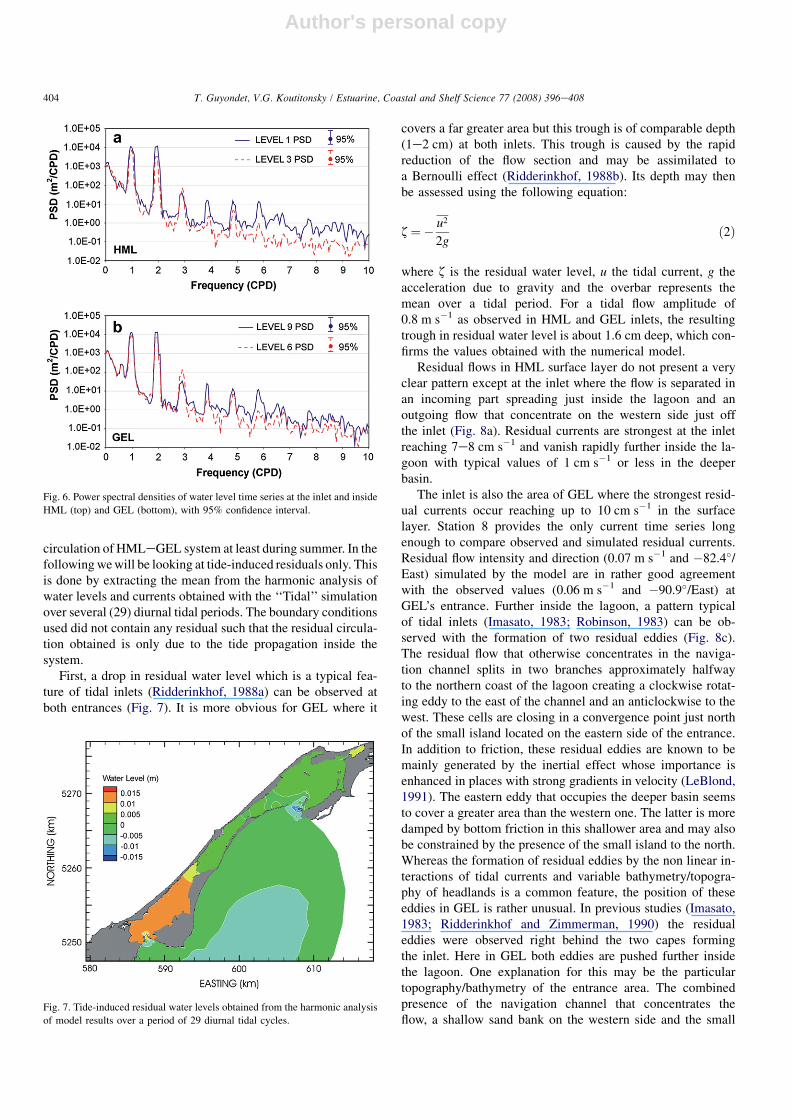
to interact either with themselves to create residuals and/orovertides or with each other to generate compound tides(Parker, 1991). Residuals will be addressed in later sections.Concerning over- and compound tides, in such a system dom-inated by M2 the first harmonic expected is the overtide M4(Aubrey and Speer, 1985). But here surprisingly the amplituderatio M4/M2 never exceeds 4%. However as mentioned aboveO1 and K1 being important constituents as well, their interac-tions with M2 lead to the generation of the compound tidesMO3 and MK3, the only harmonics reaching a noticeablemagnitude (Fig. 5e,f; MO3 not shown as very similar toMK3). Here a small fraction of the energy of the major constit-uents seems to be transferred to compound tides (MO3 andMK3). These components see a slight increase in amplitudeas the tide propagates inside both lagoons (Fig. 5e). This trans-fer of energy induced by non-linear processes such as bed fric-tion and/or tide/bathymetry interactions is slightly stronger inGEL as the tidal wave travels over the shallow internal throatsection. Comparison of power spectral density (PSD) of waterlevel fluctuations (Percival and Walden, 1993) between en-trances and inner stations (Fig. 6) confirms the overall energydecrease of the signal due to friction and also shows explicitlythe transfer of part of the energy lost by diurnal and semi-diurnal constituents to ter-diurnal species. This transfer ismaximum at the junction between both lagoons (as seen in

harmonic analysis results, Table 1) where the signal is themost affected by non-linear shalow water processes and tidalconstituent interactions.

The model seems to reproduce this non-linear generationquite accurately as amplitude and phase of MK3 observed atstation 5 (0.026 m and 233�) compare reasonably well withthe ones obtained with the model in this area (0.02e0.03 mand 210e220�). Other interactions between O1 and K1, M2and O1 and M2 and K1 may generate compound tides of thesame frequency as M2, K1 and O1 respectively. Each of thesecompound tides would then be masked by the astronomicalconstituent of same frequency which possess a much largeramplitude.

To complete this overview of the system’s tidal dynamics itcan be noticed from the time series of Fig. 3c,d that HML’s en-trance exhibits maximum ebb and flood currents of approxi-mately the same strength whereas GEL’s mouth encountersan asymmetrical pattern,with maximum currents being consis-tently stronger at ebb. This tidal asymmetry and the absence ofthe M4 constituent noticed above could seem paradoxal. Butas mentioned in previous studies (Ranasinghe and Pattiaratchi,2000; Hoitink et al., 2003; van Maren et al., 2004) in systemswhere semi-diurnal and diurnal signals are of the same orderof magnitude a tidal asymmetry may arise from the direct in-teraction between M2, O1 and K1 rather than from overtides

Fig. 4. Model results for the surface layer tidal currents in maximum flood (a, b) and ebb conditions (c, d). The vector colour represents the velocity magnitude

following the colour scale shown.

402 T. Guyondet, V.G. Koutitonsky / Estuarine, Coastal and Shelf Science 77 (2008) 396e408

Author's personal copy

generated by shallow water processes and friction, a morecommon mechanism in systems dominated by semi-diurnalspecies (Aubrey and Speer, 1985; Speer and Aubrey, 1985;Fry and Aubrey, 1990).

3.3. Residual flows and water levels

Residual flows are of greater interest than tidal currents forthe transport of dissolved or suspended matter as they inform

about long term circulation patterns and fate of the transportedmatter. Residual flows in coastal systems are mainly generatedby non-linear interactions between tidal constituents and coastaltopography and bathymetry (tide-induced), wind stress, densitygradients, fresh water inflows and external water level gradientsfor multiple inlet systems (Uncles, 1982; Feng et al., 1986b;Smith, 1990 and others). As mentioned earlier, fresh waterinflows are not an issue here and the assumption was madethat density gradients do not play a major role in the water

Fig. 5. Results of the harmonic analysis of water level time series over the whole domain area for the main constituents M2, O1 and the compound tide MK3.

403T. Guyondet, V.G. Koutitonsky / Estuarine, Coastal and Shelf Science 77 (2008) 396e408

Author's personal copy

circulation of HMLeGEL system at least during summer. In thefollowing we will be looking at tide-induced residuals only. Thisis done by extracting the mean from the harmonic analysis ofwater levels and currents obtained with the ‘‘Tidal’’ simulationover several (29) diurnal tidal periods. The boundary conditionsused did not contain any residual such that the residual circula-tion obtained is only due to the tide propagation inside thesystem.

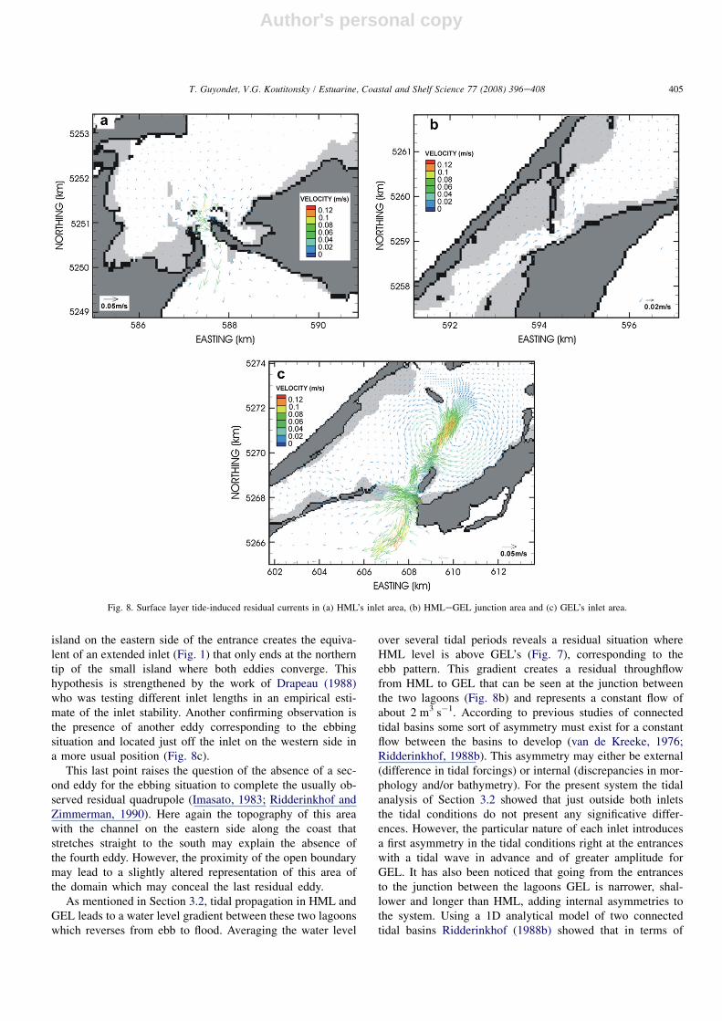
First, a drop in residual water level which is a typical fea-ture of tidal inlets (Ridderinkhof, 1988a) can be observed atboth entrances (Fig. 7). It is more obvious for GEL where it

covers a far greater area but this trough is of comparable depth(1e2 cm) at both inlets. This trough is caused by the rapidreduction of the flow section and may be assimilated toa Bernoulli effect (Ridderinkhof, 1988b). Its depth may thenbe assessed using the following equation:

z¼� u2

2gð2Þ

where z is the residual water level, u the tidal current, g theacceleration due to gravity and the overbar represents themean over a tidal period. For a tidal flow amplitude of0.8 m s�1 as observed in HML and GEL inlets, the resultingtrough in residual water level is about 1.6 cm deep, which con-firms the values obtained with the numerical model.

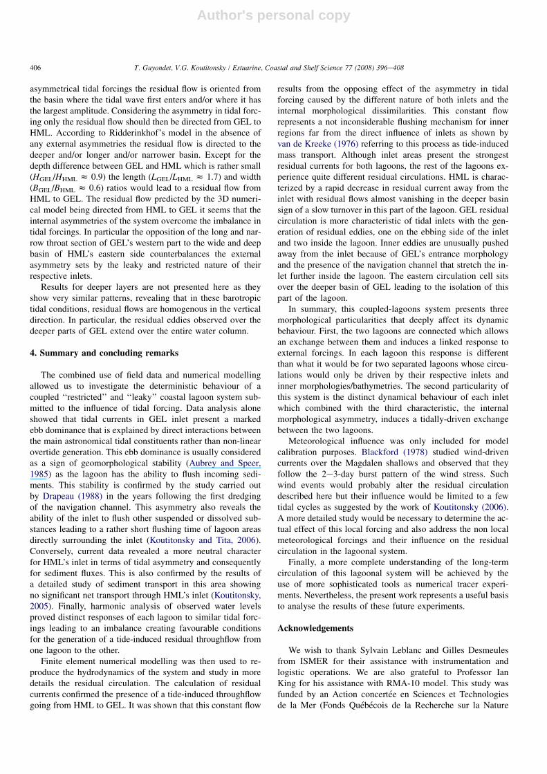
Residual flows in HML surface layer do not present a veryclear pattern except at the inlet where the flow is separated inan incoming part spreading just inside the lagoon and anoutgoing flow that concentrate on the western side just offthe inlet (Fig. 8a). Residual currents are strongest at the inletreaching 7e8 cm s�1 and vanish rapidly further inside the la-goon with typical values of 1 cm s�1 or less in the deeperbasin.

The inlet is also the area of GEL where the strongest resid-ual currents occur reaching up to 10 cm s�1 in the surfacelayer. Station 8 provides the only current time series longenough to compare observed and simulated residual currents.Residual flow intensity and direction (0.07 m s�1 and �82.4�/East) simulated by the model are in rather good agreementwith the observed values (0.06 m s�1 and �90.9�/East) atGEL’s entrance. Further inside the lagoon, a pattern typicalof tidal inlets (Imasato, 1983; Robinson, 1983) can be ob-served with the formation of two residual eddies (Fig. 8c).The residual flow that otherwise concentrates in the naviga-tion channel splits in two branches approximately halfwayto the northern coast of the lagoon creating a clockwise rotat-ing eddy to the east of the channel and an anticlockwise to thewest. These cells are closing in a convergence point just northof the small island located on the eastern side of the entrance.In addition to friction, these residual eddies are known to bemainly generated by the inertial effect whose importance isenhanced in places with strong gradients in velocity (LeBlond,1991). The eastern eddy that occupies the deeper basin seemsto cover a greater area than the western one. The latter is moredamped by bottom friction in this shallower area and may alsobe constrained by the presence of the small island to the north.Whereas the formation of residual eddies by the non linear in-teractions of tidal currents and variable bathymetry/topogra-phy of headlands is a common feature, the position of theseeddies in GEL is rather unusual. In previous studies (Imasato,1983; Ridderinkhof and Zimmerman, 1990) the residualeddies were observed right behind the two capes formingthe inlet. Here in GEL both eddies are pushed further insidethe lagoon. One explanation for this may be the particulartopography/bathymetry of the entrance area. The combinedpresence of the navigation channel that concentrates theflow, a shallow sand bank on the western side and the small

Fig. 6. Power spectral densities of water level time series at the inlet and inside

HML (top) and GEL (bottom), with 95% confidence interval.

Fig. 7. Tide-induced residual water levels obtained from the harmonic analysis

of model results over a period of 29 diurnal tidal cycles.

404 T. Guyondet, V.G. Koutitonsky / Estuarine, Coastal and Shelf Science 77 (2008) 396e408

Author's personal copy

island on the eastern side of the entrance creates the equiva-lent of an extended inlet (Fig. 1) that only ends at the northerntip of the small island where both eddies converge. Thishypothesis is strengthened by the work of Drapeau (1988)who was testing different inlet lengths in an empirical esti-mate of the inlet stability. Another confirming observation isthe presence of another eddy corresponding to the ebbingsituation and located just off the inlet on the western side ina more usual position (Fig. 8c).

This last point raises the question of the absence of a sec-ond eddy for the ebbing situation to complete the usually ob-served residual quadrupole (Imasato, 1983; Ridderinkhof andZimmerman, 1990). Here again the topography of this areawith the channel on the eastern side along the coast thatstretches straight to the south may explain the absence ofthe fourth eddy. However, the proximity of the open boundarymay lead to a slightly altered representation of this area ofthe domain which may conceal the last residual eddy.

As mentioned in Section 3.2, tidal propagation in HML andGEL leads to a water level gradient between these two lagoonswhich reverses from ebb to flood. Averaging the water level

over several tidal periods reveals a residual situation whereHML level is above GEL’s (Fig. 7), corresponding to theebb pattern. This gradient creates a residual throughflowfrom HML to GEL that can be seen at the junction betweenthe two lagoons (Fig. 8b) and represents a constant flow ofabout 2 m3 s�1. According to previous studies of connectedtidal basins some sort of asymmetry must exist for a constantflow between the basins to develop (van de Kreeke, 1976;Ridderinkhof, 1988b). This asymmetry may either be external(difference in tidal forcings) or internal (discrepancies in mor-phology and/or bathymetry). For the present system the tidalanalysis of Section 3.2 showed that just outside both inletsthe tidal conditions do not present any significative differ-ences. However, the particular nature of each inlet introducesa first asymmetry in the tidal conditions right at the entranceswith a tidal wave in advance and of greater amplitude forGEL. It has also been noticed that going from the entrancesto the junction between the lagoons GEL is narrower, shal-lower and longer than HML, adding internal asymmetries tothe system. Using a 1D analytical model of two connectedtidal basins Ridderinkhof (1988b) showed that in terms of

Fig. 8. Surface layer tide-induced residual currents in (a) HML’s inlet area, (b) HMLeGEL junction area and (c) GEL’s inlet area.

405T. Guyondet, V.G. Koutitonsky / Estuarine, Coastal and Shelf Science 77 (2008) 396e408

Author's personal copy

asymmetrical tidal forcings the residual flow is oriented fromthe basin where the tidal wave first enters and/or where it hasthe largest amplitude. Considering the asymmetry in tidal forc-ing only the residual flow should then be directed from GEL toHML. According to Ridderinkhof’s model in the absence ofany external asymmetries the residual flow is directed to thedeeper and/or longer and/or narrower basin. Except for thedepth difference between GEL and HML which is rather small(HGEL/HHML z 0.9) the length (LGEL/LHML z 1.7) and width(BGEL/BHML z 0.6) ratios would lead to a residual flow fromHML to GEL. The residual flow predicted by the 3D numeri-cal model being directed from HML to GEL it seems that theinternal asymmetries of the system overcome the imbalance intidal forcings. In particular the opposition of the long and nar-row throat section of GEL’s western part to the wide and deepbasin of HML’s eastern side counterbalances the externalasymmetry sets by the leaky and restricted nature of theirrespective inlets.

Results for deeper layers are not presented here as theyshow very similar patterns, revealing that in these barotropictidal conditions, residual flows are homogenous in the verticaldirection. In particular, the residual eddies observed over thedeeper parts of GEL extend over the entire water column.

4. Summary and concluding remarks

The combined use of field data and numerical modellingallowed us to investigate the deterministic behaviour of acoupled ‘‘restricted’’ and ‘‘leaky’’ coastal lagoon system sub-mitted to the influence of tidal forcing. Data analysis aloneshowed that tidal currents in GEL inlet present a markedebb dominance that is explained by direct interactions betweenthe main astronomical tidal constituents rather than non-linearovertide generation. This ebb dominance is usually consideredas a sign of geomorphological stability (Aubrey and Speer,1985) as the lagoon has the ability to flush incoming sedi-ments. This stability is confirmed by the study carried outby Drapeau (1988) in the years following the first dredgingof the navigation channel. This asymmetry also reveals theability of the inlet to flush other suspended or dissolved sub-stances leading to a rather short flushing time of lagoon areasdirectly surrounding the inlet (Koutitonsky and Tita, 2006).Conversely, current data revealed a more neutral characterfor HML’s inlet in terms of tidal asymmetry and consequentlyfor sediment fluxes. This is also confirmed by the results ofa detailed study of sediment transport in this area showingno significant net transport through HML’s inlet (Koutitonsky,2005). Finally, harmonic analysis of observed water levelsproved distinct responses of each lagoon to similar tidal forc-ings leading to an imbalance creating favourable conditionsfor the generation of a tide-induced residual throughflow fromone lagoon to the other.

Finite element numerical modelling was then used to re-produce the hydrodynamics of the system and study in moredetails the residual circulation. The calculation of residualcurrents confirmed the presence of a tide-induced throughflowgoing from HML to GEL. It was shown that this constant flow

results from the opposing effect of the asymmetry in tidalforcing caused by the different nature of both inlets and theinternal morphological dissimilarities. This constant flowrepresents a not inconsiderable flushing mechanism for innerregions far from the direct influence of inlets as shown byvan de Kreeke (1976) referring to this process as tide-inducedmass transport. Although inlet areas present the strongestresidual currents for both lagoons, the rest of the lagoons ex-perience quite different residual circulations. HML is charac-terized by a rapid decrease in residual current away from theinlet with residual flows almost vanishing in the deeper basinsign of a slow turnover in this part of the lagoon. GEL residualcirculation is more characteristic of tidal inlets with the gen-eration of residual eddies, one on the ebbing side of the inletand two inside the lagoon. Inner eddies are unusually pushedaway from the inlet because of GEL’s entrance morphologyand the presence of the navigation channel that stretch the in-let further inside the lagoon. The eastern circulation cell sitsover the deeper basin of GEL leading to the isolation of thispart of the lagoon.

In summary, this coupled-lagoons system presents threemorphological particularities that deeply affect its dynamicbehaviour. First, the two lagoons are connected which allowsan exchange between them and induces a linked response toexternal forcings. In each lagoon this response is differentthan what it would be for two separated lagoons whose circu-lations would only be driven by their respective inlets andinner morphologies/bathymetries. The second particularity ofthis system is the distinct dynamical behaviour of each inletwhich combined with the third characteristic, the internalmorphological asymmetry, induces a tidally-driven exchangebetween the two lagoons.

Meteorological influence was only included for modelcalibration purposes. Blackford (1978) studied wind-drivencurrents over the Magdalen shallows and observed that theyfollow the 2e3-day burst pattern of the wind stress. Suchwind events would probably alter the residual circulationdescribed here but their influence would be limited to a fewtidal cycles as suggested by the work of Koutitonsky (2006).A more detailed study would be necessary to determine the ac-tual effect of this local forcing and also address the non localmeteorological forcings and their influence on the residualcirculation in the lagoonal system.

Finally, a more complete understanding of the long-termcirculation of this lagoonal system will be achieved by theuse of more sophisticated tools as numerical tracer experi-ments. Nevertheless, the present work represents a useful basisto analyse the results of these future experiments.

Acknowledgements

We wish to thank Sylvain Leblanc and Gilles Desmeulesfrom ISMER for their assistance with instrumentation andlogistic operations. We are also grateful to Professor IanKing for his assistance with RMA-10 model. This study wasfunded by an Action concertee en Sciences et Technologiesde la Mer (Fonds Quebecois de la Recherche sur la Nature

406 T. Guyondet, V.G. Koutitonsky / Estuarine, Coastal and Shelf Science 77 (2008) 396e408

Author's personal copy

et les Technologies) grant to V.K. et al., by ISMER, by RAQ(Reseau Aquaculture Quebec) and by SODIM (Societe deDeveloppement de l’Industrie Maricole). The 2001 field mea-surements were part of a contract study by V.K. for GenivarLtd. and funded by the Quebec Ministry of Transport.

Appendix. RMA-10 numerical model equations

Momentum:

r

�vu

vtþ u

vu

vxþ v

vu

vyþw

vu

vz

�� v

vx

�3xx

vu

vx

�� v

vy

�3xy

vu

vy

�

� v

vz

�3xz

vu

vz

�þ vp

vx�Gx ¼ 0

r

�vv

vtþ u

vv

vxþ v

vv

vyþw

vv

vz

�� v

vx

�3yx

vv

vx

�� v

vy

�3yy

vv

vy

�

� v

vz

�3yz

vv

vz

�þ vp

vy�Gy ¼ 0

r

�vw

vtþ u

vw

vxþ v

vw

vyþw

vw

vz

�� v

vx

�3zx

vw

vx

�� v

vy

�3zy

vw

vy

�

� v

vz

�3zz

vw

vz

�þ vp

vzþ rg�Gz ¼ 0

using the hydrostatic approximation the momentum equationin the vertical direction is reduced to:

vp

vzþ rg¼ 0

Continuity:

vu

vxþ vv

vyþ vw

vz¼ 0

Transport of heat and/or salinity (salinity used as an example):

vs

vtþ u

vs

vxþ v

vs

vyþw

vs

vz� v

vx

�Dx

vs

vx

�� v

vy

�Dy

vs

vy

�

� v

vz

�Dz

vs

vz

�� qs ¼ 0

Equation of state:

r¼ FðSÞ

with: x, y, z: cartesian coordinates, z being the ascendant ver-tical; u, v, w: velocities in the cartesian directions; r: waterdensity; g: acceleration due to gravity; p: water pressure;3xx.: turbulent eddy coefficients; G: external tractions thatoperate on the boundaries or on the interior; S: salinity;Dx.: eddy diffusion coefficients; qs: source/sink for the trans-ported variable.

References

Aubrey, D.G., Speer, P.E., 1985. A Study of Non-linear Tidal Propagation in

shallow Inlet/Estuarine Systems. Part I: Observations. Estuarine, Coastal

and Shelf Science 21, 185e205.

Aubrey, D.G., McSherry, T.R., Eliet, P.P., 1993. Effects of multiple inlet mor-

phology on tidal exchange: Waquoit Bay, Massachusetts. In: Aubrey, D.G.,

Giese, G.S. (Eds.), Formation and Evolution of Multiple Tidal Inlets.

Coastal and Estuarine Studies, vol. 44. American Geophysical Union,

Washington, pp. 213e235.

Blackford, B.L., 1978. Wind-driven inertial currents in the Magdalen

Shallows, Gulf of St. Lawrence. Journal of Physical Oceanography

8, 653e664.

Booth, D., 1994. Tidal flushing of semi-enclosed bays. In: Beven, K.,

Chatwin, P., Millbank, J. (Eds.), Mixing and Transport in the Environment.

John Wiley & Sons, New York, pp. 203e219.

DiLorenzo, J.L., 1988. The overtide and filtering response of small inlet/bay

systems. In: Aubrey, D.G., Weishar, L. (Eds.), Hydrodynamics and Sedi-

ment Dynamics of Tidal Inlets. Lecture Notes on Coastal and Estuarine

Studies, vol. 29. Springer, New York, pp. 24e53.

Drapeau, G., 1988. Stability of tidal inlet navigation channels and adjacent

dredge spoil islands. In: Aubrey, D.G., Weishar, L. (Eds.), Hydrodynamics

and Sediment Dynamics of Tidal Inlets. Lecture Notes on Coastal and

Estuarine Studies, vol. 29. Springer, New York, pp. 226e244.

Dronkers, J., Zimmerman, J.T.F., 1982. Some principles of mixing in tidal

lagoons. Oceanologica Acta SP, 107e117.

Feng, S., Cheng, R.T., Xi, P., 1986a. On tide-induced lagrangian residual

current and residual transport. 1. Lagrangian residual Current. Water

Resources Research 22, 1623e1634.

Feng, S., Cheng, R.T., Xi, P., 1986b. On tide-induced lagrangian residual

current and residual transport. 2. Residual transport with application in

South San Francisco Bay, California. Water Resources Research 22,

1635e1646.

Foreman, M.G., 1977. Manual for tidal heights analysis and previsions. Pacific

Marine Science Report 77-10.

Fortunato, A.B., Oliveira, A., 2005. Influence of intertidal flats on tidal

asymmetry. Journal of Coastal Research 21, 1062e1067.

Fry, V.A., Aubrey, D.G., 1990. Tidal velocity asymmetries and bedload

transport in shallow embayments. Estuarine, Coastal and Shelf Science

30, 453e473.

Hoitink, A.J.F., Hoekstra, P., van Maren, D.S., 2003. Flow asymmetry

associated with astronomical tides: Implications for the residual transport

of sediment. Journal of Geophysical Research 108 (13), 1e8.

Imasato, N., 1983. What is tide-induced residual current? Journal of Physical

Oceanography 13, 1307e1317.

Janzen, C.D., Wong, K.-C., 1998. On the low-frequency transport processes in

a shallow coastal lagoon. Estuaries 21, 754e766.

Jones, J.E., Davies, A.M., 2007. On the sensitivity of tidal residuals off the

west coast of Britain to mesh resolution. Continental Shelf Research 27,

64e81.

Keulegan, G.H., 1967. Tidal Flow in Entrances, Water-Level Fluctuations of

Basins in Communication with Seas, Committee on Tidal Hydraulics,

Corps of Engineers, U.S. Army, Vicksburg, Mississippi.

King, I.P., 1982. A Finite Element Model for Three Dimensional Flow, report

prepared by Resource Management Associates, Lafayette California, for

U.S. Army Corps of Engineers, Waterways Experiment Station, Vicksburg,

Mississippi.

King, I.P., 1985. Strategies for finite element modeling of three dimensional

hydrodynamic systems. Advances in Water Resources 8, 69e76.

King, I., 1993. RMA-10. A Finite Element Model for Three-Dimensional Den-

sity Stratified Flow. Department of Civil and Environmental Engineering.

University of California, Davis.

Kjerfve, B., 1986. Comparative oceanography of coastal lagoons. In: Wolfe, D.A.

(Ed.), Estuarine Variability. Academic Press, New York, pp. 63e81.

Kjerfve, B., Knoppers, B.A., 1991. Tidal choking in a coastal lagoon.

In: Parker, B.B. (Ed.), Tidal Hydrodynamics. Wiley, New York, pp.

169e181.

407T. Guyondet, V.G. Koutitonsky / Estuarine, Coastal and Shelf Science 77 (2008) 396e408

Author's personal copy

Koutitonsky, V.G., 2005. Modelisation numerique integree des courants, des

vagues et du transport des sediments a l’entree de la lagune de Havre-

aux-Maisons, Rapport de recherche LHE-05-2. Laboratoire d’hydraulique

environnementale. ISMER, Rimouski, Qc. 151 p.

Koutitonsky, V.G., 2006. Three-dimensional structure of wind-driven currents

in coastal lagoons. In: Gonenc, I.E., Wolfin, J.P. (Eds.), Coastal Lagoons:

Ecosystem Processes and Modeling for Sustainable Use and Development.

CRC Press, pp. 376e391.

Koutitonsky, V.G., Tita, G., 2006. Temps de renouvellement des eaux dans

la lagune de Grande-Entree aux Iles-de-la-Madeleine., Ministere de

l’Agriculture, des Pecheries et de l’Alimentation du Quebec. Cahier

d’information no. 151. 73 pp.

Koutitonsky, V.G., Navarro, N., Booth, D., 2002. Descriptive physical ocean-

ography of Great-Entry Lagoon, Gulf of St. Lawrence. Estuarine, Coastal

and Shelf Science 54, 833e847.

van de Kreeke, J., 1976. Tide-induced mass transport: A flushing mechanism

for shallow lagoons. Journal of Hydraulic Research 14, 61e67.

van de Kreeke, J., 1988. Hydrodynamics of tidal inlets. In: Aubrey, D.G.,

Weishar, L. (Eds.), Hydrodynamics and Sediment Dynamics of Tidal

Inlets. Lecture Notes on Coastal and Estuarine Studies, vol. 29. Springer,

New York, pp. 1e23.

LeBlond, P.H., 1991. Tides and their interactions with other oceanographic

phenomena in shallow water (Review). In: Parker, B.B. (Ed.), Tidal

Hydrodynamics. Wiley, New York, pp. 125e152.

Lee, J.C., Davies, A.M., 1999. Open boundary and frictional influences in 3D

tidal models. Journal of Hydraulic Engineering 125, 1084e1096.

Legrand, S., Deleersnijder, E., Hanert, E., Legat, V., Wolanski, E., 2006. High-

resolution, unstructured meshes for hydrodynamic models of the Great

Barrier Reef, Australia. Estuarine, Coastal and Shelf Science 68, 36e46.

Loder, J.W., Shen, Y., Ridderinkhof, H., 1997. Characterization of three-

dimensional Lagrangian circulation associated with tidal rectification over

a submarine bank. Journal of Physical Oceanography 27, 1729e1742.

Longuet-Higgins, M.S., 1969. On the transport of mass by time-varying ocean

currents. Deep-Sea Research 16, 431e447.

van Maren, D.S., Hoekstra, P., Hoitink, A.J.F., 2004. Tidal flow asymmetry in

the diurnal regime: bed-load transport and morphologic changes around

the Red River Delta. Ocean Dynamics 54, 424e434.

Parker, B.B., 1991. The relative importance of the various nonlinear mecha-

nisms in a wide range of tidal interactions (Review). In: Parker, B.B.

(Ed.), Tidal Hydrodynamics. Wiley, New York, pp. 237e268.

Percival, D.B., Walden, A.T., 1993. Spectral Analysis for Physical Applica-

tions: Multitaper and Conventional Univariate Techniques. Cambridge

University Press, Cambridge.

Prandle, D., 1991. Tides in estuaries and embayments (Review). In: Parker, B.B.

(Ed.), Tidal Hydrodynamics. Wiley, New York, pp. 125e152.

Ranasinghe, R., Pattiaratchi, C., 2000. Tidal inlet velocity asymmetry in

diurnal regimes. Continental Shelf Research 20, 2347e2366.

Ridderinkhof, H., 1988a. Tidal and residual flows in the western Dutch Wad-

den Sea. I: Numerical model results. Netherlands Journal of Sea Research

22, 1e21.

Ridderinkhof, H., 1988b. Tidal and residual flows in the western Dutch

Wadden Sea. II: An analytical model to study the constant flow be-

tween connected tidal basins. Netherlands Journal of Sea Research

22, 185e198.

Ridderinkhof, H., Loder, J.W., 1994. Lagrangian characterization of circula-

tion over submarine banks with application to the outer Gulf of Maine.

Journal of Physical Oceanography 24, 1184e1200.

Ridderinkhof, H., Zimmerman, J.T.F., 1990. Residual currents in the Western

Dutch Wadden Sea. In: Cheng, R.T. (Ed.), Residual Currents and Long-

Term Transport. Coastal and Estuarine Studies, vol. 38. Springer, New

York, pp. 93e104.

Robinson, I.S., 1983. Tidally induced residual flows. In: Johns, B. (Ed.),

Physical Oceanography of Coastal and Shelf Seas. Elsevier Oceanography

Series, Amsterdam.

Salles, P., Voulgaris, G., Aubrey, D.G., 2005. Contribution of nonlinear mech-

anisms in the persistence of multiple tidal inlet systems. Estuarine, Coastal

and Shelf Science 65, 475e491.

Shetye, S.R., Gouveia, A.D., 1992. On the role of geometry of cross-section in

generating flood-dominance in shallow estuaries. Estuarine, Coastal and

Shelf Science 35, 113e126.

Smagorinsky, J., 1963. General circulation experiment with the primitive

equations. Monthly Weather Review 91, 99e164.

Smith, N.P., 1990. Wind domination of residual tidal transport in a coastal

lagoon. In: Cheng, R.T. (Ed.), Residual Currents and Long-Term Trans-

port. Coastal and Estuarine Studies, vol. 38. Springer, New York, pp.

121e133.

Speer, P.E., Aubrey, D.G., 1985. A study of non-linear tidal propagation in

shallow inlet/estuarine systems. Part II: Theory. Estuarine, Coastal and

Shelf Science 21, 207e224.

Tee, K.-T., Lefaivre, D., 1990. Three-dimensional modeling of the tidally

induced residual circulation off Southwest Nova Scotia. In: Cheng, R.T.

(Ed.), Residual Currents and Long-Term Transport. Coastal and Estuarine

Studies, vol. 38. Springer, New York, pp. 79e92.

Uncles, R.J., 1982. Computed and observed residual currents in the Bristol

Channel. Oceanologica Acta 5, 11e20.

Wei, H., Hainbucher, D., Pohlmann, T., Feng, S., Suendermann, J., 2004.

Tidal-induced Lagrangian and Eulerian mean circulation in the Bohai

Sea. Journal of Marine Systems 44, 141e151.

Zimmerman, J.T.F., 1981. Dynamics, diffusion and geomorphological signifi-

cance of tidal residual eddies. Nature 290, 549e555.

408 T. Guyondet, V.G. Koutitonsky / Estuarine, Coastal and Shelf Science 77 (2008) 396e408