An Overview of the Usefulness and Strategic Value of Rare Earth ...
Upload
independentCategory
view
0download
0
Ta
MJa
b
a
ARRA
KCMsM2ML
1
igbmDm
1h
Ecological Indicators 29 (2013) 48–61
Contents lists available at SciVerse ScienceDirect
Ecological Indicators
jo ur n al homep ag e: www.elsev ier .com/ locate /eco l ind
he usefulness of large body-size macroinvertebrates in the rapid ecologicalssessment of Mediterranean lagoons
aurizio Pinnaa,∗, Gabriele Marinia, Ilaria Rosati a, João M. Netob, Joana Patríciob,oão Carlos Marquesb, Alberto Basseta
Department of Biological and Environmental Sciences and Technologies, University of the Salento, S.P. Lecce-Monteroni, 73100 Lecce, ItalyIMAR – Institute of Marine Research, Department of Life Sciences, University of Coimbra, Largo Marquês de Pombal, 3004-517 Coimbra, Portugal
r t i c l e i n f o
rticle history:eceived 19 March 2012eceived in revised form 3 December 2012ccepted 6 December 2012
eywords:ost-effectiveness biomonitoringacroinvertebrates body-size based
ample selectionanual sorting time
mm mesh size sieveediterranean transitional waters
esina lagoon
a b s t r a c t
The success of a monitoring programme depends on the precision and accuracy of assessment tools, on thecosts of sampling and laboratory procedures, on the time lag between sampling and the availability of theresults. Aquatic ecosystem monitoring programmes using macroinvertebrates, developed in compliancewith the EC Water Framework Directive, are constrained by assessment tools which require economicallyexpensive activities and long time lags. This research investigates the adequacy of simplified samplingprocedures, based on the selection of large body-size macroinvertebrates, retained by a 2 mm mesh sizesieve, to detect the ecological status of a Mediterranean lagoon. To this aim, various tools for assess-ment of lagoon ecological status were compared, using three macroinvertebrate datasets obtained byfield sieving with 2 mm, 1 mm and 0.5 mm sizes of mesh sieves. Simple community descriptors (numer-ical density, taxonomic richness, biomass density and individual body-size), taxonomic diversity indices(Shannon–Weaver, Margalef, Pielou, Average Taxonomic Distinctness) and ecological indicators sensuWFD (AMBI, BENTIX, BITS, M-AMBI) were used as assessment tools. In September 2009, three soft bot-tom samples of 0.1 m2 were collected, sieved through the column of sieves, at seven study sites locatedalong a Total Pressure gradient of Lesina lagoon (Italy). Three datasets were obtained with the macroin-vertebrates retained by the 2 mm mesh sieve (2mm), the 1 mm and 2 mm sieves (1mm) and the 0.5 mm,1 mm and 2 mm sieves (0.5mm). The manual sorting time was also recorded for each sample and com-pared across the three datasets. Taxonomic richness, numerical and biomass densities were significantlyhigher in the 0.5mm than the 1mm and 2mm datasets, as expected. Nevertheless, the ecological indicatorsclassified the study sites in the same EQS class with all datasets in 64% of cases; comparing the 2mm and0.5mm datasets, the 2mm and 1mm datasets and the 0.5mm and 1mm datasets, the percentages were 64%,
80% and 86%, respectively. Individual body-size, AMBI, BENTIX were significantly correlated with TotalPressure at each dataset, M-AMBI at 1mm and 2mm and biomass density only at 2mm. The manual sor-ting time was 56% shorter for the large body-size macroinvertebrate fraction than for the 1mm, and 72%shorter than for the 0.5mm. Finally, the larger body-size macroinvertebrates seem to be advantageousand useful for accurate, rapid and cost effective biomonitoring. Further investigations to define referenceare s
conditions for each mesh. Introduction
The environmental policy of the European Union concern-ng the management and protection of water bodies attributes areater role in ecological quality assessment to aquatic ecosystemiological components than to physical, chemical and hydro-
orphological approaches. The Water Framework Directive (WFD,irective 2000/60/EC) cites biological quality elements such as theain ecosystem components and requires the development and∗ Corresponding author. Tel.: +39 0832298604; fax: +39 0832298626.E-mail address: [email protected] (M. Pinna).
470-160X/$ – see front matter © 2012 Elsevier Ltd. All rights reserved.ttp://dx.doi.org/10.1016/j.ecolind.2012.12.011
till needed, mainly for body-size based ecological indicators.© 2012 Elsevier Ltd. All rights reserved.
validation of assessment tools to determine the ecological qual-ity status of European aquatic ecosystems. The ecological qualitystatus (EQS) of water bodies can be assessed by the application ofspecific metrics, simple and/or multiple, based on the abundance,taxonomic composition and body-size based descriptors, in oneor more biological quality elements (phytoplankton, zooplankton,macrophytes, macroinvertebrates and fish) (Pinto et al., 2009; Pontiet al., 2009). Alternative and/or combined metrics, traits and abi-otic parameters are required for the calculation of assessment tools.
Assessment tools are based on: (1) taxonomic composition, abun-dance and species sensitivity (Shannon and Weaver, 1963; Clarkeand Warwick, 1998; Borja et al., 2000; Simboura and Zenetos, 2002;Basset et al., 2008; Orfanidis et al., 2008); (2) body-size based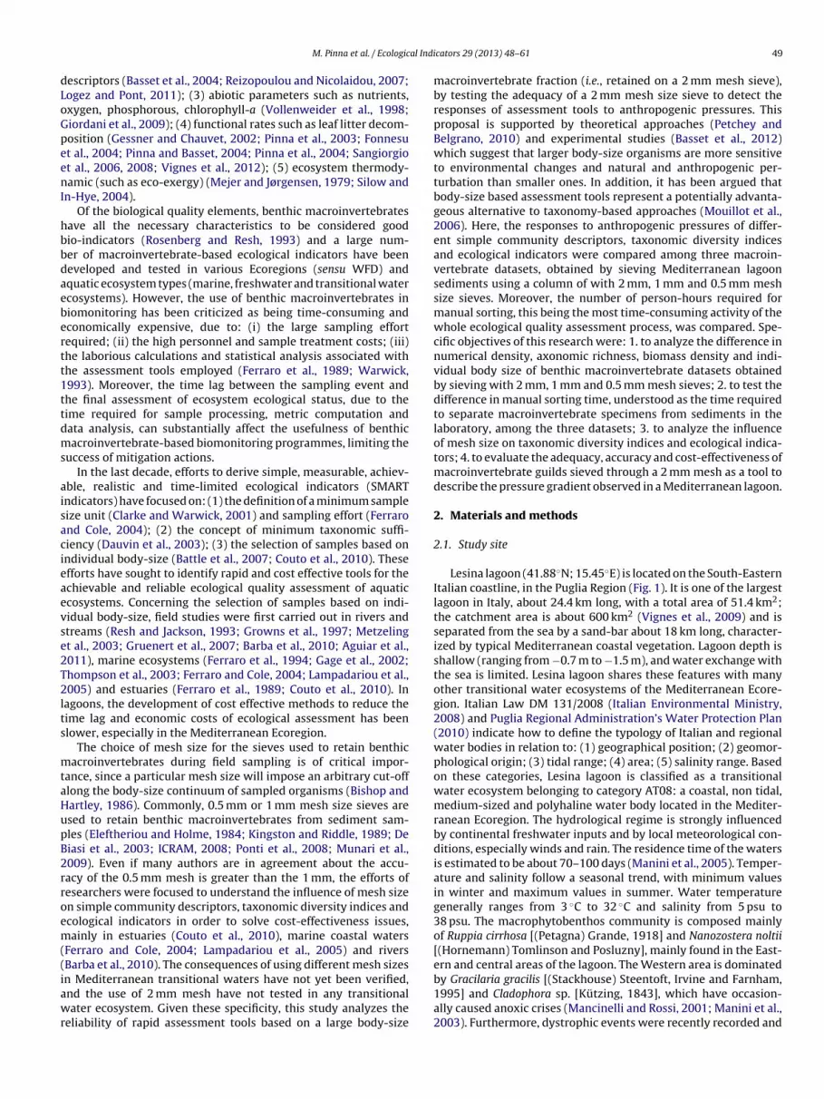
al Indi
dLoGpeenI
hbbdaebertt1ttdms
aisacieaevse2T2lts
mtaHupB2rroem((iawr
M. Pinna et al. / Ecologic
escriptors (Basset et al., 2004; Reizopoulou and Nicolaidou, 2007;ogez and Pont, 2011); (3) abiotic parameters such as nutrients,xygen, phosphorous, chlorophyll-a (Vollenweider et al., 1998;iordani et al., 2009); (4) functional rates such as leaf litter decom-osition (Gessner and Chauvet, 2002; Pinna et al., 2003; Fonnesut al., 2004; Pinna and Basset, 2004; Pinna et al., 2004; Sangiorgiot al., 2006, 2008; Vignes et al., 2012); (5) ecosystem thermody-amic (such as eco-exergy) (Mejer and Jørgensen, 1979; Silow and
n-Hye, 2004).Of the biological quality elements, benthic macroinvertebrates
ave all the necessary characteristics to be considered goodio-indicators (Rosenberg and Resh, 1993) and a large num-er of macroinvertebrate-based ecological indicators have beeneveloped and tested in various Ecoregions (sensu WFD) andquatic ecosystem types (marine, freshwater and transitional watercosystems). However, the use of benthic macroinvertebrates iniomonitoring has been criticized as being time-consuming andconomically expensive, due to: (i) the large sampling effortequired; (ii) the high personnel and sample treatment costs; (iii)he laborious calculations and statistical analysis associated withhe assessment tools employed (Ferraro et al., 1989; Warwick,993). Moreover, the time lag between the sampling event andhe final assessment of ecosystem ecological status, due to theime required for sample processing, metric computation andata analysis, can substantially affect the usefulness of benthicacroinvertebrate-based biomonitoring programmes, limiting the
uccess of mitigation actions.In the last decade, efforts to derive simple, measurable, achiev-
ble, realistic and time-limited ecological indicators (SMARTndicators) have focused on: (1) the definition of a minimum sampleize unit (Clarke and Warwick, 2001) and sampling effort (Ferrarond Cole, 2004); (2) the concept of minimum taxonomic suffi-iency (Dauvin et al., 2003); (3) the selection of samples based onndividual body-size (Battle et al., 2007; Couto et al., 2010). Thesefforts have sought to identify rapid and cost effective tools for thechievable and reliable ecological quality assessment of aquaticcosystems. Concerning the selection of samples based on indi-idual body-size, field studies were first carried out in rivers andtreams (Resh and Jackson, 1993; Growns et al., 1997; Metzelingt al., 2003; Gruenert et al., 2007; Barba et al., 2010; Aguiar et al.,011), marine ecosystems (Ferraro et al., 1994; Gage et al., 2002;hompson et al., 2003; Ferraro and Cole, 2004; Lampadariou et al.,005) and estuaries (Ferraro et al., 1989; Couto et al., 2010). In
agoons, the development of cost effective methods to reduce theime lag and economic costs of ecological assessment has beenlower, especially in the Mediterranean Ecoregion.
The choice of mesh size for the sieves used to retain benthicacroinvertebrates during field sampling is of critical impor-
ance, since a particular mesh size will impose an arbitrary cut-offlong the body-size continuum of sampled organisms (Bishop andartley, 1986). Commonly, 0.5 mm or 1 mm mesh size sieves aresed to retain benthic macroinvertebrates from sediment sam-les (Eleftheriou and Holme, 1984; Kingston and Riddle, 1989; Deiasi et al., 2003; ICRAM, 2008; Ponti et al., 2008; Munari et al.,009). Even if many authors are in agreement about the accu-acy of the 0.5 mm mesh is greater than the 1 mm, the efforts ofesearchers were focused to understand the influence of mesh sizen simple community descriptors, taxonomic diversity indices andcological indicators in order to solve cost-effectiveness issues,ainly in estuaries (Couto et al., 2010), marine coastal waters
Ferraro and Cole, 2004; Lampadariou et al., 2005) and riversBarba et al., 2010). The consequences of using different mesh sizes
n Mediterranean transitional waters have not yet been verified,nd the use of 2 mm mesh have not tested in any transitionalater ecosystem. Given these specificity, this study analyzes theeliability of rapid assessment tools based on a large body-size
cators 29 (2013) 48–61 49
macroinvertebrate fraction (i.e., retained on a 2 mm mesh sieve),by testing the adequacy of a 2 mm mesh size sieve to detect theresponses of assessment tools to anthropogenic pressures. Thisproposal is supported by theoretical approaches (Petchey andBelgrano, 2010) and experimental studies (Basset et al., 2012)which suggest that larger body-size organisms are more sensitiveto environmental changes and natural and anthropogenic per-turbation than smaller ones. In addition, it has been argued thatbody-size based assessment tools represent a potentially advanta-geous alternative to taxonomy-based approaches (Mouillot et al.,2006). Here, the responses to anthropogenic pressures of differ-ent simple community descriptors, taxonomic diversity indicesand ecological indicators were compared among three macroin-vertebrate datasets, obtained by sieving Mediterranean lagoonsediments using a column of with 2 mm, 1 mm and 0.5 mm meshsize sieves. Moreover, the number of person-hours required formanual sorting, this being the most time-consuming activity of thewhole ecological quality assessment process, was compared. Spe-cific objectives of this research were: 1. to analyze the difference innumerical density, axonomic richness, biomass density and indi-vidual body size of benthic macroinvertebrate datasets obtainedby sieving with 2 mm, 1 mm and 0.5 mm mesh sieves; 2. to test thedifference in manual sorting time, understood as the time requiredto separate macroinvertebrate specimens from sediments in thelaboratory, among the three datasets; 3. to analyze the influenceof mesh size on taxonomic diversity indices and ecological indica-tors; 4. to evaluate the adequacy, accuracy and cost-effectiveness ofmacroinvertebrate guilds sieved through a 2 mm mesh as a tool todescribe the pressure gradient observed in a Mediterranean lagoon.
2. Materials and methods
2.1. Study site
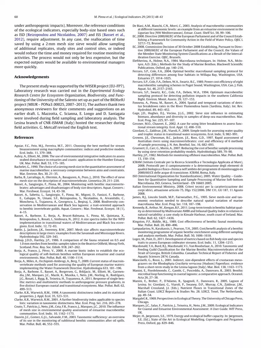
Lesina lagoon (41.88◦N; 15.45◦E) is located on the South-EasternItalian coastline, in the Puglia Region (Fig. 1). It is one of the largestlagoon in Italy, about 24.4 km long, with a total area of 51.4 km2;the catchment area is about 600 km2 (Vignes et al., 2009) and isseparated from the sea by a sand-bar about 18 km long, character-ized by typical Mediterranean coastal vegetation. Lagoon depth isshallow (ranging from −0.7 m to −1.5 m), and water exchange withthe sea is limited. Lesina lagoon shares these features with manyother transitional water ecosystems of the Mediterranean Ecore-gion. Italian Law DM 131/2008 (Italian Environmental Ministry,2008) and Puglia Regional Administration’s Water Protection Plan(2010) indicate how to define the typology of Italian and regionalwater bodies in relation to: (1) geographical position; (2) geomor-phological origin; (3) tidal range; (4) area; (5) salinity range. Basedon these categories, Lesina lagoon is classified as a transitionalwater ecosystem belonging to category AT08: a coastal, non tidal,medium-sized and polyhaline water body located in the Mediter-ranean Ecoregion. The hydrological regime is strongly influencedby continental freshwater inputs and by local meteorological con-ditions, especially winds and rain. The residence time of the watersis estimated to be about 70–100 days (Manini et al., 2005). Temper-ature and salinity follow a seasonal trend, with minimum valuesin winter and maximum values in summer. Water temperaturegenerally ranges from 3 ◦C to 32 ◦C and salinity from 5 psu to38 psu. The macrophytobenthos community is composed mainlyof Ruppia cirrhosa [(Petagna) Grande, 1918] and Nanozostera noltii[(Hornemann) Tomlinson and Posluzny], mainly found in the East-ern and central areas of the lagoon. The Western area is dominated
by Gracilaria gracilis [(Stackhouse) Steentoft, Irvine and Farnham,1995] and Cladophora sp. [Kützing, 1843], which have occasion-ally caused anoxic crises (Mancinelli and Rossi, 2001; Manini et al.,2003). Furthermore, dystrophic events were recently recorded and
50 M. Pinna et al. / Ecological Indicators 29 (2013) 48–61
an coa
s2p
2
c(tsstte0autslftd2fi(Owsdqbsp
TGi
Fig. 1. Map of Lesina lagoon (South-Eastern Itali
tudied in the south-western part of the lagoon (Specchiulli et al.,009; Vignes et al., 2009), which is therefore considered the mosterturbed part of the lagoon (Borja et al., 2011).
.2. Sampling and laboratory procedures
Sediment samples containing benthic macroinvertebrates wereollected in September 2009 at seven study sites in Lesina lagoonFig. 1); sampling campaign was carried out in the framework ofhe WISER project, funded by the FP7 programme. Lesina is a veryhallow lagoon, only small boats are available and only relativelymall grabs can be used to collect sediment samples. Sampling washerefore carried out using a 15 cm × 15 cm Ekman-Birge grab fourimes per replicate. Three replicates per study site were collected;ach replicate covered a sampling surface area of approximately.1 m2, as suggested by ISO (2005). The study sites were locatedlong the main axis of the lagoon and were the same as thosesed in the study by Borja et al. (2011). The main abiotic fea-ures and pressures of the study sites are shown in Table 1. Amongtudy sites, WSL01 is located in the south-western part of theagoon and was considered the most perturbed site due to dif-use agricultural inputs, domestic and industrial discharges, andhe inputs of aquiculture; these are the main causes of periodicystrophic phenomena observed in the summer (Specchiulli et al.,009; Vignes et al., 2009; Borja et al., 2011). After collection in theeld, each replicate was sieved through a column of three sieves
®Retsch, Germany) with mesh sizes of 2 mm, 1 mm and 0.5 mm.smotic stress and related body-shape variation of the organismsas avoided by using field pre-filtered water (0.125 mm mesh
ieve) to remove fine sediments from the replicates. Sieves had aiameter of 40 cm and a mesh that conformed to the DIN ISO 3310/1
uality standard. The benthic macroinvertebrate samples retainedy each sieve were separately fixed in 4% buffered formalin. At eachtudy site, physical and chemical parameters (depth [cm], tem-erature [◦C], conductivity [�S/cm], salinity [psu], oxygen [mg/l],able 1eographical position and physical and chemical parameters of Lesina lagoon study site
ncreasing Total Pressure.
Study sites
WSL03 WSL04 WSL05
Latitude (N) 41◦53′09.8′′ 41◦53′20.1′′ 41◦53′32.5′′
Longitude (E) 15◦26′25.5′′ 15◦27′33.6′′ 15◦28′56.5′′
Depth (cm) −110 −110 −120
Temperature (◦C) 25.8 24.6 24.4
Conductivity (�S/cm) 20,500 19,970 20,450
Salinity (psu) 17.36 17.02 17.28
Oxygen (mg/l) 6.92 9.77 6.24
Transparency (cm) −110 −110 −120
Organic content (%) 10.4 9.4 14.0
*Total Pressure 4 4 4
stline) and geographical position of study sites.
transparency [cm] and organic content [%]) were recorded using ahand-held multiprobe (YSI 556) and a Secchi disk, organic matterwas determined in laboratory (Table 1). In the laboratory, sampleswere washed to remove formalin and benthic macroinvertebrateswere hand-separated from organic and inorganic residual sedi-ments using a stereo-microscope (Leica MZ6). The sample washingwater was stored in plastic tanks and sent for disposal. Given thatmanual sorting is a time-consuming procedure, we recorded thetime and the number of experts and non-experts needed to com-plete the sorting of each sample. Manual sorting is the laboratoryprocedure by which the macroinvertebrates are separated fromresidual sediments (after field sieving). These data were subse-quently used in the cost/benefit analysis, comparing data from2 mm, 1 mm and 0.5 mm mesh size samples. To complete the labo-ratory procedures, including taxonomic identification at the lowestpossible level, measures of total length and dry weight were madefor each specimen. Dry weight was obtained after desiccation in astove at 60 ◦C for 72 h; subsequently, the ash content was obtainedby pooling specimens of the same taxon and placing them in a muf-fle furnace at 450 ◦C for 12 h. The body-size of each specimen wasexpressed as ash free dry weight (AFDW, mg), excluding the ashcontent percentage from each specimen’s dry weight.
2.3. Anthropogenic pressures
In this research, the anthropogenic pressures of study sites werederived by Borja et al. (2011); they treated type of pressures suchas non-point pollution sources, point pollution sources, habitatloss, industry, ports and fisheries. Borja et al. (2011) quantifiedthe pressures following an approach based on “expert judgment”(Aubry and Elliott, 2006), with reference to the following levels: 1
for low; 2 for medium; 3 for high. “Total Pressure” at each study sitewas calculated as the sum of partial pressures (Borja et al., 2011).Based on the “Total Pressure” values, the relative position of thestudy sites along the pressure gradient (from low to high pressure)s. (*) Total Pressure derived by Borja et al. (2011). Study sites are listed based on
WSL07 WSL06 WSL02 WSL01
41◦54′00.3′′ 41◦53′43.2′′ 41◦52′05.8′′ 41◦51′56.6′′
15◦32′13.9′′ 15◦30′01.3′′ 15◦21′43.0′′ 15◦20′35.3′′
−60 −105 −100 −10024.4 24.4 25.0 24.016,010 19,880 22,130 22,23113.60 16.55 18.46 18.0611.15 9.59 7.59 7.59−60 −105 −100 −709.8 8.7 5.6 4.75 7 9 10
al Indi
w(stlmm
2i
ifi“b“bfiltwse(sMelaT
2
1rsttbtirwLbds
2
DAcBr(hdLtswo
M. Pinna et al. / Ecologic
as: WSL03 = WSL04 = WSL05 < WSL07 < WSL06 < WSL02 < WSL01Table 1). The Spearman rank correlations between the “Total Pres-ure” values of each study site and simple community descriptors,axonomic diversity indices and ecological indicators were ana-yzed, comparing the results obtained using the three benthic
acroinvertebrate datasets derived from 0.5 mm, 1 mm and 2 mmesh size sieves.
.4. Datasets, simple community descriptors, taxonomic diversityndices and ecological indicators
Three datasets were built up: (1) the first was called “2mm”, andncluded all specimens retained by the 2 mm mesh size sieve – therst sieve in the column used in the field; (2) the second was called1mm”, and included the 2mm dataset plus all specimens retainedy the 1 mm mesh size sieve of the column; (3) the third was called0.5mm”, and included the 1mm dataset plus all specimens retainedy the 0.5 mm mesh size sieve, which was the finest used duringeld sieving. For each specimen, taxonomic identification to the
owest possible level (LPT), functional feeding group (FFG), ash con-ent percentage and individual body-size (Ash Free Dry Weight)ere included in the relevant datasets. The FFG was assigned to
pecimens based on available literature and experts (Macdonaldt al., 2010). Simple community descriptors [numerical densityN), taxonomic richness (S), biomass density (B), individual body-ize (IBS)], taxonomic diversity indices [Shannon–Weaver (H′),argalef (D), Pielou (J′), Average Taxonomic Distinctness (AvTD)],
cological indicators (AMBI, BENTIX, BITS, M-AMBI) were calcu-ated for each replicate and mesh size, and averaged for study sitesnd mesh size. Specific formulas and descriptions are shown inable 2.
.5. Manual sorting time
The manual sorting time per sample was recorded for the 2 mm, mm and 0.5 mm mesh sieve replicates, separately. For the 2 mmeplicates, the manual sorting time was recorded directly; the 1 mmorting time was obtained as the sum of the 2 mm sorting time andhe 1 mm time; the 0.5 mm manual sorting time was obtained ashe sum of the 2 mm, 1 mm and 0.5 mm sorting times. The num-er of person hours required per sample was normalized accordingo the experience of the persons using expert evaluations, allocat-ng a correction factor of 1 to expert researchers and 0.5 to youngesearchers still in training. The efficiency and accuracy of all stepsere validated by a control group made up of expert researchers.
inear regressions were performed to analyze the relationshipetween manual sorting time per sample with simple communityescriptors. Differences among 0.5 mm, 1 mm and 2 mm manualorting time per sample were tested using one-way ANOVA.
.6. Computation and statistical analysis
The taxonomic diversity indices were calculated using theIVERSE tool from PRIMER 6 software, using loge to compute H′.MBI (Borja et al., 2000) and M-AMBI (Muxika et al., 2007) werealculated using AMBI index software 4.1 (http://ambi.azti.es).ENTIX (Simboura and Zenetos, 2002) was calculated witheference to http://www.hcmr.gr/listview3.php?id=1195. BITSMistri and Munari, 2008) was calculated with reference tottp://www.bits.unife.it. For this index, reference EQR values wereefined using the classes corresponding to sand habitats, since inesina lagoon the percentage of sand in the sediment is higher than
hat of mud (Borja et al., 2011) (Table 2). The ecological qualitytatus (EQS) of the seven study sites was derived in accordanceith the WFD for all ecological indicators to compare the responsesf the three datasets. Here, the results of the simple community
cators 29 (2013) 48–61 51
descriptors, taxonomic diversity indices and ecological indicatorsobtained at replicate level in the 2mm, 1mm and 0.5mm datasetsand averaged for study site/mesh size were compared. Differencesin simple community descriptors, taxonomic diversity indices andecological indicators among mesh sizes and among study sites wereanalyzed using a one-way ANOVA, followed by a post hoc test. Posthoc tests were carried out using the Turkey (HSD) test. Moreover,to take into account the type I error (rejected H0 when it is true)due to multiple tests, p-values were adjusted according to Bonfer-roni correction. It was carried out after data exploration accordingto Zuur et al. (2010) and transforming data as X1/3, in order toreach the normality assumptions. The normality was tested usingKolmogorov–Smirnov test. Significant values were considered forp < 0.05. Hereafter, study sites were ordered in an increasing pres-sure gradient according to preliminary classification (Borja et al.,2011). The variation of simple community descriptors, taxonomicdiversity indices and ecological indicators with Total Pressure ineach study site were analyzed within each dataset using Spear-man rank correlation. All statistical analyses were performed usingthe software STATISTICA 8. Bray–Curtis coefficient was calculatedto test taxonomic similarity among study sites for 0.5mm, 1mmand 2mm datasets using PRIMER software, and the differenceswere tested by means of one-way ANOVA. It was calculated takenthe average of pairwise dissimilarity percentage values betweenstudy sites. Finally, the performance of each sieve mesh size wasestablished as the efficiency percentage obtained by pairwise com-parison of the results obtained for all assessment tools using the0.5mm, 1mm and 2mm datasets.
3. Results
3.1. Description of benthic macroinvertebrate guilds
In total (0.5mm dataset), 47,127 benthic macroinvertebrateswere sampled from the seven study sites; 22 taxa were identi-fied, including 15 to species level, 3 to genus level, 2 to familylevel and 2 to subclass level (Table 3). The 1mm dataset contained23,324 benthic macroinvertebrates; 21 taxa were identified, 15 ofwhich to species level (Table 3). The specimens retained by the2 mm mesh sieve during field sieving procedures (2mm dataset)included 5,200 benthic macroinvertebrates; 17 taxa were iden-tified to the lowest possible level (with 14 identified to specieslevel) (Table 3). In the 2mm dataset, total abundance amounted to23% of what was observed in the 1mm dataset and 11% of whatwas observed in the 0.5mm dataset. The number of taxa sam-pled with the 2 mm mesh was 81% of the figure observed withthe 1mm dataset, and 77% of the figure observed with the 0.5mmdataset. Most taxa were found in all three datasets; only Hirudinea,Oligochaeta, Spionidae and Capitella capitata were restricted tothe 1mm and 0.5mm datasets, and Corophium sp. was restrictedto the 0.5mm dataset (with a single specimen). These taxa seemto be retained specifically by 1 mm or 0.5 mm meshes, but theywere extremely rare in terms of numerical density (Table 3), andtheir spatial distribution was extremely restricted (being found in1, 3, 1, 1 and 1 study sites, respectively). In the 0.5mm dataset,Ecrobia ventrosa accounted for about 84% of specimens, while 16taxa collectively accounted for less than 1% (Fig. 2A; Table 3).In this dataset, E. ventrosa was the smallest species in terms ofaverage individual body-size and was the dominant species at allstudy sites, among which the taxonomic Bray–Curtis similaritycoefficient was relatively high (65.07 ± 2.773). In the 1mm dataset,approximately 85% of benthic macroinvertebrates belonged to
only three taxa; specifically, 72% were E. ventrosa, 7.7% were Abrasegmentum and 5.3% were Mytilaster minimus, while 12 taxa collec-tively accounted for less than 1% (Fig. 2A; Table 3). E. ventrosa wasthe dominant species at each study site, as with the 0.5mm dataset,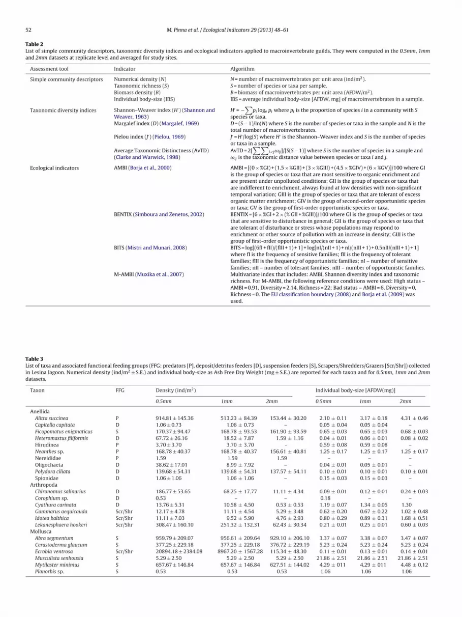
52 M. Pinna et al. / Ecological Indicators 29 (2013) 48–61
Table 2List of simple community descriptors, taxonomic diversity indices and ecological indicators applied to macroinvertebrate guilds. They were computed in the 0.5mm, 1mmand 2mm datasets at replicate level and averaged for study sites.
Assessment tool Indicator Algorithm
Simple community descriptors Numerical density (N) N = number of macroinvertebrates per unit area (ind/m2).Taxonomic richness (S) S = number of species or taxa per sample.Biomass density (B) B = biomass of macroinvertebrates per unit area (AFDW/m2).Individual body-size (IBS) IBS = average individual body-size [AFDW, mg] of macroinvertebrates in a sample.
Taxonomic diversity indices Shannon–Weaver index (H′) (Shannon andWeaver, 1963)
H′ = −∑
pi loge pi where pi is the proportion of species i in a community with Sspecies or taxa.
Margalef index (D) (Margalef, 1969) D = (S − 1)/ln(N) where S is the number of species or taxa in the sample and N is thetotal number of macroinvertebrates.
Pielou index (J′) (Pielou, 1969) J′ = H′/log(S) where H′ is the Shannon–Weaver index and S is the number of speciesor taxa in a sample.
Average Taxonomic Distinctness (AvTD)(Clarke and Warwick, 1998)
AvTD = 2[∑∑
i<jωij]/[S(S − 1)] where S is the number of species in a sample andωij is the taxonomic distance value between species or taxa i and j.
Ecological indicators AMBI (Borja et al., 2000) AMBI = [(0 × %GI) + (1.5 × %GII) + (3 × %GIII) + (4.5 × %GIV) + (6 × %GV)]/100 where GIis the group of species or taxa that are most sensitive to organic enrichment andare present under unpolluted conditions; GII is the group of species or taxa thatare indifferent to enrichment, always found at low densities with non-significanttemporal variation; GIII is the group of species or taxa that are tolerant of excessorganic matter enrichment; GIV is the group of second-order opportunistic speciesor taxa; GV is the group of first-order opportunistic species or taxa.
BENTIX (Simboura and Zenetos, 2002) BENTIX = [6 × %GI + 2 × (% GII + %GIII)]/100 where GI is the group of species or taxathat are sensitive to disturbance in general; GII is the group of species or taxa thatare tolerant of disturbance or stress whose populations may respond toenrichment or other source of pollution with an increase in density; GIII is thegroup of first-order opportunistic species or taxa.
BITS (Mistri and Munari, 2008) BITS = log[(6fI + fII)/(fIII + 1) + 1] + log[nI/(nII + 1) + nI/(nIII + 1) + 0.5nII/(nIII + 1) + 1]where fI is the frequency of sensitive families; fII is the frequency of tolerantfamilies; fIII is the frequency of opportunistic families; nI – number of sensitivefamilies; nII – number of tolerant families; nIII – number of opportunistic families.
M-AMBI (Muxika et al., 2007) Multivariate index that includes: AMBI, Shannon diversity index and taxonomicrichness. For M-AMBI, the following reference conditions were used: High status –AMBI = 0.91, Diversity = 2.14, Richness = 22; Bad status – AMBI = 6, Diversity = 0,Richness = 0. The EU classification boundary (2008) and Borja et al. (2009) wasused.
Table 3List of taxa and associated functional feeding groups (FFG: predators [P], deposit/detritus feeders [D], suspension feeders [S], Scrapers/Shredders/Grazers [Scr/Shr]) collectedin Lesina lagoon. Numerical density (ind/m2 ± S.E.) and individual body-size as Ash Free Dry Weight (mg ± S.E.) are reported for each taxon and for 0.5mm, 1mm and 2mmdatasets.
Taxon FFG Density (ind/m2) Individual body-size [AFDW(mg)]
0.5mm 1mm 2mm 0.5mm 1mm 2mm
AnellidaAlitta succinea P 914.81 ± 145.36 513.23 ± 84.39 153.44 ± 30.20 2.10 ± 0.11 3.17 ± 0.18 4.31 ± 0.46Capitella capitata D 1.06 ± 0.73 1.06 ± 0.73 – 0.05 ± 0.04 0.05 ± 0.04 –Ficopomatus enigmaticus S 170.37 ± 94.47 168.78 ± 93.53 161.90 ± 93.59 0.65 ± 0.03 0.65 ± 0.03 0.68 ± 0.03Heteromastus filiformis D 67.72 ± 26.16 18.52 ± 7.87 1.59 ± 1.16 0.04 ± 0.01 0.06 ± 0.01 0.08 ± 0.02Hirudinea P 3.70 ± 3.70 3.70 ± 3.70 - 0.59 ± 0.08 0.59 ± 0.08 –Neanthes sp. P 168.78 ± 40.37 168.78 ± 40.37 156.61 ± 40.81 1.25 ± 0.17 1.25 ± 0.17 1.25 ± 0.17Nereididae P 1.59 1.59 1.59 – – –Oligochaeta D 38.62 ± 17.01 8.99 ± 7.92 – 0.04 ± 0.01 0.05 ± 0.01 –Polydora ciliata D 139.68 ± 54.31 139.68 ± 54.31 137.57 ± 54.11 0.10 ± 0.01 0.10 ± 0.01 0.10 ± 0.01Spionidae D 1.06 ± 1.06 1.06 ± 1.06 – 0.15 ± 0.03 0.15 ± 0.03 –
ArthropodaChironomus salinarius D 186.77 ± 53.65 68.25 ± 17.77 11.11 ± 4.34 0.09 ± 0.01 0.12 ± 0.01 0.24 ± 0.03Corophium sp. D 0.53 – – 0.18 – –Cyathura carinata D 13.76 ± 5.31 10.58 ± 4.50 0.53 ± 0.53 1.19 ± 0.07 1.34 ± 0.05 1.30Gammarus aequicauda Scr/Shr 12.17 ± 4.78 11.11 ± 4.54 5.29 ± 3.48 0.62 ± 0.20 0.67 ± 0.22 1.02 ± 0.48Idotea balthica Scr/Shr 11.11 ± 7.03 9.52 ± 5.90 4.76 ± 2.93 0.80 ± 0.29 0.89 ± 0.31 1.68 ± 0.51Lekanesphaera hookeri Scr/Shr 308.47 ± 160.10 251.32 ± 132.31 62.43 ± 30.34 0.21 ± 0.01 0.25 ± 0.01 0.60 ± 0.03
MolluscaAbra segmentum S 959.79 ± 209.07 956.61 ± 209.64 929.10 ± 206.10 3.37 ± 0.07 3.38 ± 0.07 3.47 ± 0.07Cerastoderma glaucum S 377.25 ± 229.18 377.25 ± 229.18 376.72 ± 229.19 5.23 ± 0.24 5.23 ± 0.24 5.23 ± 0.24Ecrobia ventrosa Scr/Shr 20894.18 ± 2384.08 8967.20 ± 1567.28 115.34 ± 48.30 0.11 ± 0.01 0.13 ± 0.01 0.14 ± 0.01Musculista senhousia S 5.29 ± 2.50 5.29 ± 2.50 5.29 ± 2.50 21.86 ± 2.51 21.86 ± 2.51 21.86 ± 2.51Mytilaster minimus S 657.67 ± 146.84 657.67 ± 146.84 627.51 ± 144.02 4.29 ± 011 4.29 ± 011 4.48 ± 0.12Planorbis sp. S 0.53 0.53 0.53 1.06 1.06 1.06
M. Pinna et al. / Ecological Indicators 29 (2013) 48–61 53
0
10
20
30
40
50
60
70
80
90
100
0.5mm 1mm 2mm
Rel
ativ
e ab
unda
nce
(%)
Others
Cerastoderma glaucum
Mytilaster minimus
Alitta succinea
Abra segmentum
Ecrobia ventrosa
A
0
10
20
30
40
50
60
70
80
90
100
0.5mm 1mm 2mm
Rel
ativ
e ab
unda
nce
(%)
Mesh size
Others
Cerastoderma glaucum
Mytilaster minimus
Musculista senhousia
B
Fs
asoltvcBtFdlo
fdsseawed1(fewso
3d
rd(
2%
4%9%
85%
0.5mm
Deposit/Detrit us fee ders
Predators
Suspension fee ders
Scrapers/Shredders/G raze rs
2%
6%
17%
75%
1mm
Deposit/Detrit us fee ders
Predators
Suspension fee ders
Scrapers/Shredders/G raze rs
6%
11%
76%
7%
2 mm
Deposit/Detrit us fee ders
Predators
Suspension fee ders
Scrapers/Shredders/G raze rs
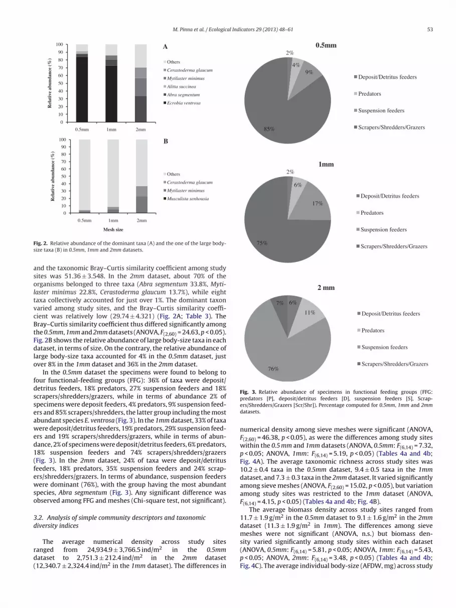
Fig. 3. Relative abundance of specimens in functional feeding groups (FFG:
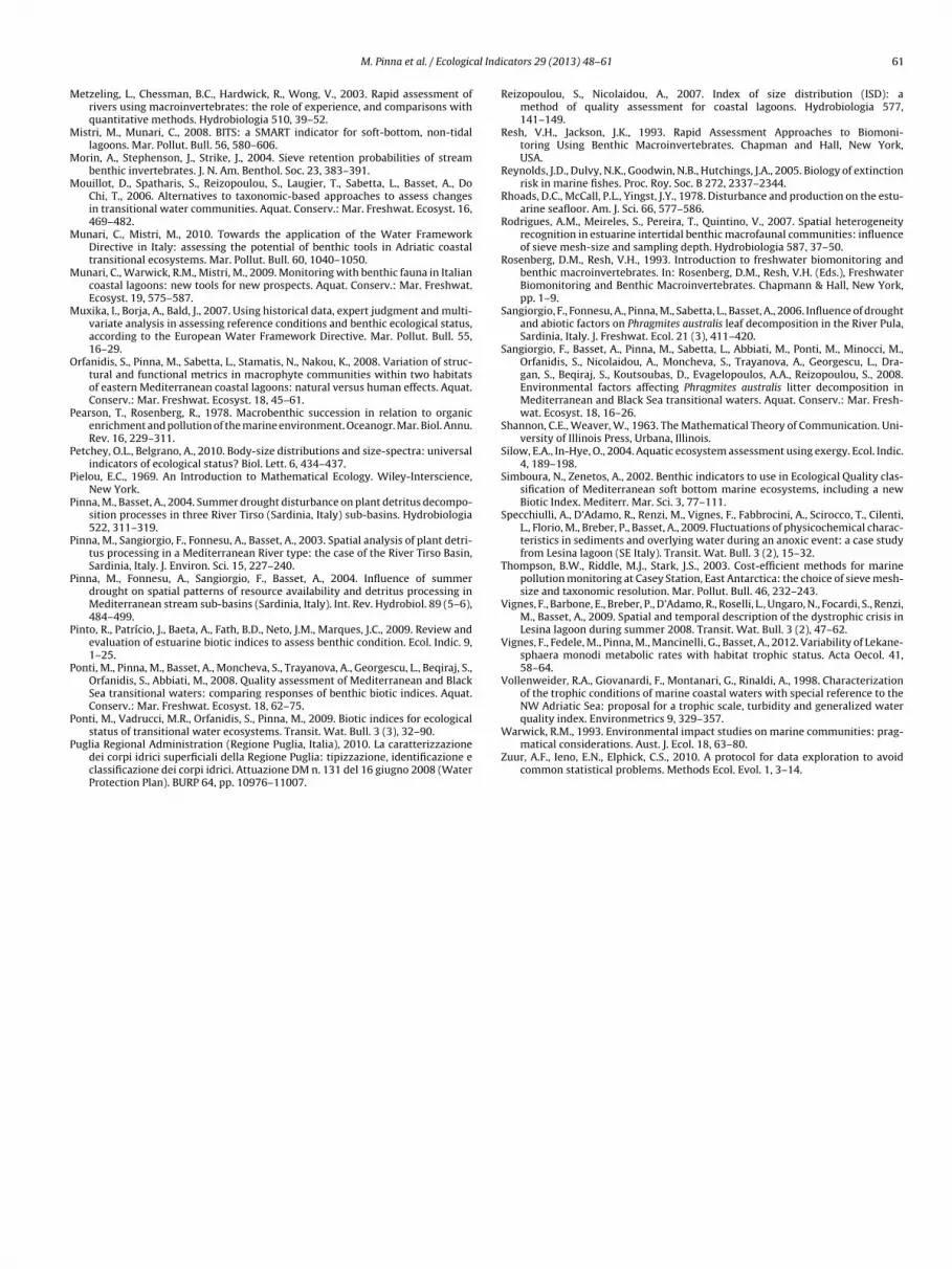
ig. 2. Relative abundance of the dominant taxa (A) and the one of the large body-ize taxa (B) in 0.5mm, 1mm and 2mm datasets.
nd the taxonomic Bray–Curtis similarity coefficient among studyites was 51.36 ± 3.548. In the 2mm dataset, about 70% of therganisms belonged to three taxa (Abra segmentum 33.8%, Myti-
aster minimus 22.8%, Cerastoderma glaucum 13.7%), while eightaxa collectively accounted for just over 1%. The dominant taxonaried among study sites, and the Bray–Curtis similarity coeffi-ient was relatively low (29.74 ± 4.321) (Fig. 2A; Table 3). Theray–Curtis similarity coefficient thus differed significantly amonghe 0.5mm, 1mm and 2mm datasets (ANOVA, F(2,60) = 24.63, p < 0.05).ig. 2B shows the relative abundance of large body-size taxa in eachataset, in terms of size. On the contrary, the relative abundance of
arge body-size taxa accounted for 4% in the 0.5mm dataset, justver 8% in the 1mm dataset and 36% in the 2mm dataset.
In the 0.5mm dataset the specimens were found to belong toour functional-feeding groups (FFG): 36% of taxa were deposit/etritus feeders, 18% predators, 27% suspension feeders and 18%crapers/shredders/grazers, while in terms of abundance 2% ofpecimens were deposit feeders, 4% predators, 9% suspension feed-rs and 85% scrapers/shredders, the latter group including the mostbundant species E. ventrosa (Fig. 3). In the 1mm dataset, 33% of taxaere deposit/detritus feeders, 19% predators, 29% suspension feed-
rs and 19% scrapers/shredders/grazers, while in terms of abun-ance, 2% of specimens were deposit/detritus feeders, 6% predators,8% suspension feeders and 74% scrapers/shredders/grazersFig. 3). In the 2mm dataset, 24% of taxa were deposit/detrituseeders, 18% predators, 35% suspension feeders and 24% scrap-rs/shredders/grazers. In terms of abundance, suspension feedersere dominant (76%), with the group having the most abundant
pecies, Abra segmentum (Fig. 3). Any significant difference wasbserved among FFG and meshes (Chi-square test, not significant).
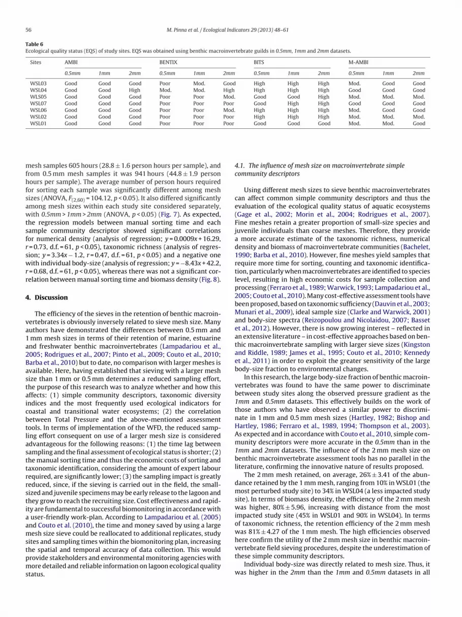
.2. Analysis of simple community descriptors and taxonomiciversity indices
The average numerical density across study sitesanged from 24,934.9 ± 3,766.5 ind/m2 in the 0.5mmataset to 2,751.3 ± 212.4 ind/m2 in the 2mm dataset12,340.7 ± 2,324.4 ind/m2 in the 1mm dataset). The differences in
predators [P], deposit/detritus feeders [D], suspension feeders [S], Scrap-ers/Shredders/Grazers [Scr/Shr]). Percentage computed for 0.5mm, 1mm and 2mmdatasets.
numerical density among sieve meshes were significant (ANOVA,F(2,60) = 46.38, p < 0.05), as were the differences among study siteswithin the 0.5 mm and 1mm datasets (ANOVA, 0.5mm: F(6,14) = 7.32,p < 0.05; ANOVA, 1mm: F(6,14) = 5.19, p < 0.05) (Tables 4a and 4b;Fig. 4A). The average taxonomic richness across study sites was10.2 ± 0.4 taxa in the 0.5mm dataset, 9.4 ± 0.5 taxa in the 1mmdataset, and 7.3 ± 0.3 taxa in the 2mm dataset. It varied significantlyamong sieve meshes (ANOVA, F(2,60) = 15.02, p < 0.05), but variationamong study sites was restricted to the 1mm dataset (ANOVA,F(6,14) = 4.15, p < 0.05) (Tables 4a and 4b; Fig. 4B).
The average biomass density across study sites ranged from11.7 ± 1.9 g/m2 in the 0.5mm dataset to 9.1 ± 1.6 g/m2 in the 2mmdataset (11.3 ± 1.9 g/m2 in 1mm). The differences among sievemeshes were not significant (ANOVA, n.s.) but biomass den-
sity varied significantly among study sites within each dataset(ANOVA, 0.5mm: F(6,14) = 5.81, p < 0.05; ANOVA, 1mm: F(6,14) = 5.43,p < 0.05; ANOVA, 2mm: F(6,14) = 3.48, p < 0.05) (Tables 4a and 4b;Fig. 4C). The average individual body-size (AFDW, mg) across study
54 M. Pinna et al. / Ecological Indicators 29 (2013) 48–61
Table 4aOne-way ANOVA and Turkey post hoc tests were carried out for simple community descriptors, taxonomic diversity indices and ecological indicators. Differences amongmesh sizes were analyzed for each study site and were supported by post hoc; p < 0.05 indicates significant tests, n.s. indicates non-significant tests. In post hoc significanttests (p < 0.05) are reported using the higher mesh size.
Site Post hoc Simple community descriptors Diversity indices Ecological indicators
N S B IBS H′ D J′ AvTD AMBI BENTIX BITS M-AMBI
WSL01 p < 0.05 n.s. p < 0.05 p < 0.05 p < 0.05 n.s. p < 0.05 n.s. n.s. n.s. n.s. n.s.0.5 mm vs 1 mm n.s. n.s. n.s. n.s. n.s.0.5 mm vs 2 mm 0.5 mm 0.5 mm 2 mm 2 mm 2 mm1 mm vs 2 mm 1 mm 1 mm 2 mm 2 mm 2 mm
WSL02 p < 0.05 p < 0.05 n.s. p < 0.05 n.s. n.s. n.s. n.s. p < 0.05 p < 0.05 p < 0.05 n.s.0.5 mm vs 1 mm n.s. 0.5 mm n.s. n.s. n.s. 1 mm0.5 mm vs 2 mm 0.5 mm 0.5 mm n.s. 0.5 mm 2 mm 0.5 mm1 mm vs 2 mm 1 mm n.s. 2 mm n.s. n.s. n.s.
WSL03 p < 0.05 n.s. p < 0.05 p < 0.05 p < 0.05 n.s. p < 0.05 n.s. p < 0.05 p < 0.05 n.s. n.s.0.5 mm vs 1 mm 0.5 mm n.s. n.s. 1 mm 1 mm n.s. n.s.0.5 mm vs 2 mm 0.5 mm 0.5 mm 2 mm 2 mm 2 mm 0.5 mm 2 mm1 mm vs 2 mm 1 mm 1 mm 2 mm n.s. 2 mm 1 mm 2 mm
WSL04 p < 0.05 p < 0.05 n.s. p < 0.05 p < 0.05 p < 0.05 p < 0.05 n.s. p < 0.05 p < 0.05 n.s. p < 0.050.5 mm vs 1 mm 0.5 mm n.s. n.s. 1 mm n.s. 1 mm n.s. 1 mm 1 mm0.5 mm vs 2 mm 0.5 mm 0.5 mm 2 mm n.s. 0.5 mm 2 mm 0.5 mm 2 mm 2 mm1 mm vs 2 mm 1 mm n.s. 2 mm n.s. 1 mm n.s. 1 mm 2 mm n.s.
WSL05 p < 0.05 n.s. n.s. p < 0.05 p < 0.05 n.s. p < 0.05 n.s. p < 0.05 p < 0.05 n.s. n.s.0.5 mm vs 1 mm 0.5 mm n.s. 1 mm 1 mm n.s. n.s.0.5 mm vs 2 mm 0.5 mm 2 mm 2 mm 2 mm 0.5 mm 2 mm1 mm vs 2 mm 1 mm 2 mm n.s. n.s. 1 mm 2 mm
WSL06 p < 0.05 n.s. n.s. p < 0.05 p < 0.05 n.s. p < 0.05 n.s. n.s. p < 0.05 n.s. n.s.0.5 mm vs 1 mm 0.5 mm n.s. 1 mm 1 mm n.s.0.5 mm vs 2 mm 0.5 mm 2 mm 2 mm 2 mm 2 mm1 mm vs 2 mm 1 mm 2 mm n.s. n.s. 2 mm
WSL07 p < 0.05 p < 0.05 n.s. p < 0.05 n.s. p < 0.05 n.s. p < 0.05 p < 0.05 n.s. p < 0.05 p < 0.05
si(sst(Tdi
STdsaiedss0aicfd
3
F
0.5 mm vs 1 mm 0.5 mm n.s. n.s.
0.5 mm vs 2 mm 0.5 mm 0.5 mm 2 mm1 mm vs 2 mm 1 mm 1 mm 2 mm
ites was 0.68 ± 0.012 mg in the 0.5mm dataset, 0.91 ± 0.017 mgn the 1mm dataset and 3.38 ± 0.062 mg in the 2mm datasetTables 4a and 4b; Fig. 4D). Overall, the average individual body-ize for each taxon varied between 21.9 ± 2.5 mg for Musculistaenhousia and 0.05 ± 0.004 mg for Oligochaeta. In the 2mm datasethe smallest taxon was Heteromastus filiformis (0.08 ± 0.023 mg)Table 3). Moreover, this estimate was significantly correlated withotal Pressure in each dataset; biomass density only in the 2mmataset, whereas taxonomic richness only in 1mm dataset. Numer-
cal density was never correlated with Total Pressure (Table 5).The spatial variability among study sites of the
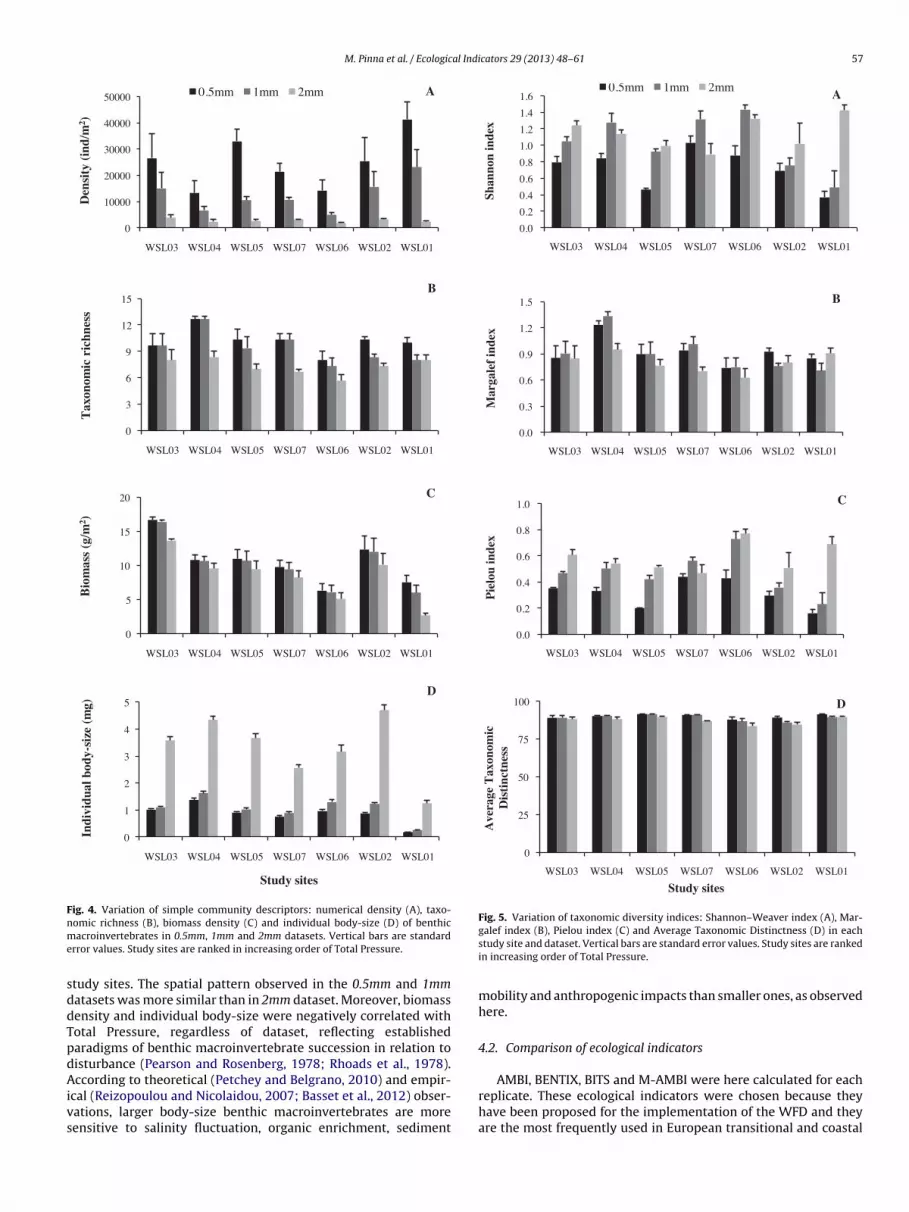
hannon–Weaver (H′), Margalef (D), Pielou (J′), and Averageaxonomic Distinctness (AvTD) taxonomic diversity indices wasescribed in the 0.5mm, 1mm and 2mm datasets (Fig. 5A–D). Thetatistical differences among study sites and among sieve meshesre shown in Tables 4a and 4b. Shannon–Weaver and Pieloundices varied significantly among sieve meshes in all study sites,xcept for WSL02 and WSL07. Margalef index was significantlyifferent only for WSL04 and WSL07, whereas AvTD was neverignificant in all study sites. Within each mesh and among studyites, Shannon–Weaver and Pielou indices varied significantly in.5 mm and 1 mm meshes, except for 2 mm mesh (Table 4b; Fig. 5And C). Margalef and AvTD indices were significantly different onlyn 1 mm mesh (Table 4b; Fig. 5B and D). Total Pressure was neverorrelated with taxonomic diversity indices in all datasets, exceptor Margalef index and Average Taxonomic Distinctness in 1mmataset (Table 5).
.3. Response of ecological indicators to pressures
AMBI values varied significantly among datasets (ANOVA,(2,60) = 10.22, p < 0.05), and were higher in the 0.5 mm than the
n.s. n.s. n.s. n.s. n.s.n.s. 0.5 mm 0.5 mm 2 mm n.s.1 mm 1 mm n.s. 2 mm 1 mm
1mm and 2mm datasets. AMBI values also varied among datasetsat all study sites considered separately except WSL01 and WSL06(Table 4a). AMBI values differed significantly among study sites,independently by mesh size used (Table 4b; Fig. 6A). They weresignificantly correlated with Total Pressure values in each dataset(Table 5). In accordance with the WFD, five EQS classes wereassigned. With AMBI, all study sites were classified as Good usingboth the 0.5mm and 1mm datasets, while using the 2mm datasetall study sites were Good except for WLS04, which was classified asHigh. The EQS results are shown in Table 6.
In contrast, the BENTIX values were significantly lower in the0.5 mm than in the 1mm and 2mm datasets (ANOVA, F(2,60) = 12.28,p < 0.05). BENTIX values also varied among datasets at all study sitesconsidered separately except for WSL01 and WSL07 (Table 4a). Sig-nificant differences among study sites were observed within eachdataset (Table 4b; Fig. 6B). BENTIX values were significantly corre-lated with Total Pressure in each dataset (Table 5). Using the 0.5mmdataset, the EQS was Poor for all sites, except for WSL04, which wasclassified as Moderate. The 1mm dataset gave the same results asthe 0.5mm dataset except for WSL03, which was classified as Mod-erate; the results obtained with the 2mm dataset provided a betterassessment for WSL03, WSL04, WLS05 and WLS06 (Table 6).
BITS values are shown in Fig. 6C. They were not correlated withTotal Pressure in any dataset (Table 5). Using the 0.5mm and 1mmdatasets, the EQS was the same in all study sites except for WSL07,which was one class better in the 1mm dataset than in the 0.5mmdataset. The 1mm and 2mm datasets classified the study sites inthe same way, except for WSL05, which was one class better in the
latter (Table 6).Finally, overall M-AMBI values did not vary significantly amongdatasets (ANOVA, n.s.). However, they did vary significantly atsites WSL01, WSL04 and WSL07 considered separately (Table 4a;
M. Pinna et al. / Ecological Indicators 29 (2013) 48–61 55
Table 4bOne-way ANOVA and Turkey post hoc tests were carried out for simple community descriptors, taxonomic diversity indices and ecological indicators. Differences amongstudy sites were analyzed for each mesh size and were supported by post hoc; p < 0.05 indicates significant tests, n.s. indicates non-significant tests. In the table, only thesignificant comparisons between study sites are reported; the first figure in each comparison indicates the higher study site.
Mesh Simple community descriptors Diversity indices Ecological indicators
N S B IBS H′ D J′ AvTD AMBI BENTIX BITS M-AMBI
0.5 mm p < 0.05 n.s. p < 0.05 p < 0.05 p < 0.05 n.s. p < 0.05 n.s. p < 0.05 p < 0.05 p < 0.05 p < 0.05Post hoc 1 4 2 1 2 1 2 1 2 1 1 3 3 1 3 1 4 1
1 6 3 1 3 1 3 1 3 1 1 4 4 1 7 15 4 2 6 4 1 4 1 4 1 2 3 3 2 4 55 6 2 7 5 1 6 1 6 1 2 4 4 2
3 6 6 1 7 1 7 1 5 3 4 37 1 4 5 3 5 6 3 3 54 2 6 5 6 5 7 3 3 64 7 7 5 7 5 5 4 3 7
6 4 4 57 4 4 6
4 7
1 mm p < 0.05 p < 0.05 p < 0.05 p < 0.05 p < 0.05 p < 0.05 p < 0.05 p < 0.05 p < 0.05 p < 0.05 p < 0.05 p < 0.05Post hoc 1 4 4 6 2 1 4 1 3 1 4 1 3 1 5 2 1 3 3 1 2 1 3 1
1 6 3 1 6 1 4 1 4 2 4 1 7 2 1 4 4 1 3 1 4 12 4 2 6 5 1 6 1 5 6 2 3 5 1 2 5 6 12 6 3 6 6 1 7 1 2 4 6 1 3 5 7 13 6 7 1 6 2 3 4 3 2 4 2
5 3 4 2 4 56 3 5 27 3 6 25 4 4 36 4 3 57 4 3 7
4 54 64 75 76 7
2 mm n.s. n.s. p < 0.05 p < 0.05 n.s. n.s. n.s. n.s. p < 0.05 p < 0.05 p < 0.05 p < 0.05Post hoc 2 1 2 1 1 3 3 1 2 1 3 2
3 1 3 1 1 4 4 1 3 1 4 24 1 4 1 2 3 6 1 6 1 3 75 1 5 1 2 4 3 2 7 1 4 77 1 6 1 3 4 4 22 6 7 1 6 3 5 2
4 7 7 3 6 25 4 4 36 4 3 57 4 3 6
3 74 54 6
FwcwAWG
TSa
ig. 6D). Significant differences were observed among study sitesithin each dataset (Table 4b). M-AMBI values were significantly
orrelated with Total Pressure in 1mm dataset and 2mm dataset,
hereas they were not correlated with 0.5mm dataset (Table 5). M-MBI-based EQS using the 0.5mm dataset was Moderate in WSL02,SL04, WSL05 and WSL07, whereas in WSL04 and WSL07 it wasood. All study sites were classified as Good in the 1mm and 2mm
able 5pearman rank correlation coefficients between Total Pressure and simple community dre reported; p < 0.05 indicates significant tests, n.s. indicates not significant tests.
Datasets Sample community descriptors Taxonomic diversity in
N S B IBS H′ D
0.5mm 0.23n.s.
−0.39n.s.
−0.33n.s.
−0.61p < 0.05
−0.24n.s.
−0.38n.s.
1mm 0.33n.s.
−0.50p < 0.05
−0.37n.s.
−0.44p < 0.05
−0.38n.s.
−0.55p < 0.05
2mm −0.25n.s.
−0.09n.s.
−0.58p < 0.05
−0.53p < 0.05
0.38n.s.
−0.08n.s.
4 75 76 7
datasets except for WSL02 and WSL05, which were classified asModerate, while WSL01 obtained a better class in the 2mm dataset.
3.4. Manual sorting time
The time to sort macroinvertebrates from all 2 mm mesh sam-ples was 264 h (12.6 ± 1.2 person hours per sample), from 1 mm
escriptors, taxonomic diversity indices and ecological indicators. The r coefficients
dices Ecological indicators
J′ AvTD AMBI BENTIX BITS M-AMBI
−0.16n.s.
0.01n.s.
0.70p < 0.05
−0.67p < 0.05
−0.25n.s.
−0.42n.s.
−0.33n.s.
−0.47p < 0.05
0.69p < 0.05
−0.68p < 0.05
0.10n.s.
−0.65p < 0.05
0.34n.s.
−0.24n.s.
0.63p < 0.05
−0.64p < 0.05
−0.16n.s.
−0.44p < 0.05
56 M. Pinna et al. / Ecological Indicators 29 (2013) 48–61
Table 6Ecological quality status (EQS) of study sites. EQS was obtained using benthic macroinvertebrate guilds in 0.5mm, 1mm and 2mm datasets.
Sites AMBI BENTIX BITS M-AMBI
0.5mm 1mm 2mm 0.5mm 1mm 2mm 0.5mm 1mm 2mm 0.5mm 1mm 2mm
WSL03 Good Good Good Poor Mod. Good High High High Mod. Good GoodWSL04 Good Good High Mod. Mod. High High High High Good Good GoodWLS05 Good Good Good Poor Poor Mod. Good Good High Mod. Mod. Mod.WSL07 Good Good Good Poor Poor Poor Good High High Good Good GoodWSL06 Good Good Good Poor Poor Mod. High High High Mod. Good GoodWSL02 Good Good Good Poor Poor Poor High High High Mod. Mod. Mod.WSL01 Good Good Good Poor Poor Poor Good Good Good Mod. Mod. Good
mfhfsawtsfrswrr
4
va1a2Bastaicbtlasttrrstiaamstpms
esh samples 605 hours (28.8 ± 1.6 person hours per sample), androm 0.5 mm mesh samples it was 941 hours (44.8 ± 1.9 personours per sample). The average number of person hours required
or sorting each sample was significantly different among meshizes (ANOVA, F(2,60) = 104.12, p < 0.05). It also differed significantlymong mesh sizes within each study site considered separately,ith 0.5mm > 1mm > 2mm (ANOVA, p < 0.05) (Fig. 7). As expected,
he regression models between manual sorting time and eachample community descriptor showed significant correlationsor numerical density (analysis of regression; y = 0.0009x + 16.29,
= 0.73, d.f. = 61, p < 0.05), taxonomic richness (analysis of regres-ion; y = 3.34x − 1.2, r = 0.47, d.f. = 61, p < 0.05) and a negative oneith individual body-size (analysis of regression; y = −8.43x + 42.2,
= 0.68, d.f. = 61, p < 0.05), whereas there was not a significant cor-elation between manual sorting time and biomass density (Fig. 8).
. Discussion
The efficiency of the sieves in the retention of benthic macroin-ertebrates is obviously inversely related to sieve mesh size. Manyuthors have demonstrated the differences between 0.5 mm and
mm mesh sizes in terms of their retention of marine, estuarinend freshwater benthic macroinvertebrates (Lampadariou et al.,005; Rodrigues et al., 2007; Pinto et al., 2009; Couto et al., 2010;arba et al., 2010) but to date, no comparison with larger meshes isvailable. Here, having established that sieving with a larger meshize than 1 mm or 0.5 mm determines a reduced sampling effort,he purpose of this research was to analyze whether and how thisffects: (1) simple community descriptors, taxonomic diversityndices and the most frequently used ecological indicators foroastal and transitional water ecosystems; (2) the correlationetween Total Pressure and the above-mentioned assessmentools. In terms of implementation of the WFD, the reduced samp-ing effort consequent on use of a larger mesh size is considereddvantageous for the following reasons: (1) the time lag betweenampling and the final assessment of ecological status is shorter; (2)he manual sorting time and thus the economic costs of sorting andaxonomic identification, considering the amount of expert labourequired, are significantly lower; (3) the sampling impact is greatlyeduced, since, if the sieving is carried out in the field, the small-ized and juvenile specimens may be early release to the lagoon andhey grow to reach the recruiting size. Cost effectiveness and rapid-ty are fundamental to successful biomonitoring in accordance with
user-friendly work-plan. According to Lampadariou et al. (2005)nd Couto et al. (2010), the time and money saved by using a largeesh size sieve could be reallocated to additional replicates, study
ites and sampling times within the biomonitoring plan, increasing
he spatial and temporal accuracy of data collection. This wouldrovide stakeholders and environmental monitoring agencies withore detailed and reliable information on lagoon ecological qualitytatus.
4.1. The influence of mesh size on macroinvertebrate simplecommunity descriptors
Using different mesh sizes to sieve benthic macroinvertebratescan affect common simple community descriptors and thus theevaluation of the ecological quality status of aquatic ecosystems(Gage et al., 2002; Morin et al., 2004; Rodrigues et al., 2007).Fine meshes retain a greater proportion of small-size species andjuvenile individuals than coarse meshes. Therefore, they providea more accurate estimate of the taxonomic richness, numericaldensity and biomass of macroinvertebrate communities (Bachelet,1990; Barba et al., 2010). However, fine meshes yield samples thatrequire more time for sorting, counting and taxonomic identifica-tion, particularly when macroinvertebrates are identified to specieslevel, resulting in high economic costs for sample collection andprocessing (Ferraro et al., 1989; Warwick, 1993; Lampadariou et al.,2005; Couto et al., 2010). Many cost-effective assessment tools havebeen proposed, based on taxonomic sufficiency (Dauvin et al., 2003;Munari et al., 2009), ideal sample size (Clarke and Warwick, 2001)and body-size spectra (Reizopoulou and Nicolaidou, 2007; Bassetet al., 2012). However, there is now growing interest – reflected inan extensive literature – in cost-effective approaches based on ben-thic macroinvertebrate sampling with larger sieve sizes (Kingstonand Riddle, 1989; James et al., 1995; Couto et al., 2010; Kennedyet al., 2011) in order to exploit the greater sensitivity of the largebody-size fraction to environmental changes.
In this research, the large body-size fraction of benthic macroin-vertebrates was found to have the same power to discriminatebetween study sites along the observed pressure gradient as the1mm and 0.5mm datasets. This effectively builds on the work ofthose authors who have observed a similar power to discrimi-nate in 1 mm and 0.5 mm mesh sizes (Hartley, 1982; Bishop andHartley, 1986; Ferraro et al., 1989, 1994; Thompson et al., 2003).As expected and in accordance with Couto et al., 2010, simple com-munity descriptors were more accurate in the 0.5mm than in the1mm and 2mm datasets. The influence of the 2 mm mesh size onbenthic macroinvertebrate assessment tools has no parallel in theliterature, confirming the innovative nature of results proposed.
The 2 mm mesh retained, on average, 26% ± 3.41 of the abun-dance retained by the 1 mm mesh, ranging from 10% in WSL01 (themost perturbed study site) to 34% in WSL04 (a less impacted studysite). In terms of biomass density, the efficiency of the 2 mm meshwas higher, 80% ± 5.96, increasing with distance from the mostimpacted study site (45% in WSL01 and 90% in WSL04). In termsof taxonomic richness, the retention efficiency of the 2 mm meshwas 81% ± 4.27 of the 1 mm mesh. The high efficiencies observedhere confirm the utility of the 2 mm mesh size in benthic macroin-
vertebrate field sieving procedures, despite the underestimation ofthese simple community descriptors.Individual body-size was directly related to mesh size. Thus, itwas higher in the 2mm than the 1mm and 0.5mm datasets in all
M. Pinna et al. / Ecological Indicators 29 (2013) 48–61 57
0
10000
20000
30000
40000
50000
WSL03 WSL04 WSL05 WSL07 WSL06 WSL02 WSL01
Den
sity
(in
d/m
2 )0.5mm 1mm 2mm A
0
3
6
9
12
15
WSL03 WSL04 WSL05 WSL07 WSL06 WSL02 WSL01
Tax
onom
ic r
ichn
ess
B
0
5
10
15
20
WSL03 WSL04 WSL05 WSL07 WSL06 WSL02 WSL01
Bio
mas
s (g
/m2 )
C
0
1
2
3
4
5
WSL03 WSL04 WSL05 WSL07 WSL06 WSL02 WSL01
Indi
vidu
al b
ody-
size
(m
g)
Stud y sites
D
Fig. 4. Variation of simple community descriptors: numerical density (A), taxo-nme
sddTpdAivs
0.0
0.2
0.4
0.6
0.8
1.0
1.2
1.4
1.6
WSL03 WSL04 WSL05 WSL07 WSL06 WSL02 WSL01
Shan
non
inde
x
A
0.0
0.3
0.6
0.9
1.2
1.5
WSL03 WSL04 WSL05 WSL07 WSL06 WSL02 WSL01
Mar
gale
f in
dex
0.5mm 1mm 2mm
B
0.0
0.2
0.4
0.6
0.8
1.0
WSL03 WSL04 WSL05 WSL07 WSL06 WSL02 WSL01
Pie
lou
inde
x C
0
25
50
75
100
WSL03 WSL04 WSL05 WSL07 WSL06 WSL02 WSL01
Ave
rage
Tax
onom
ic
Dis
tinc
tnes
s
Study sites
D
Fig. 5. Variation of taxonomic diversity indices: Shannon–Weaver index (A), Mar-
omic richness (B), biomass density (C) and individual body-size (D) of benthicacroinvertebrates in 0.5mm, 1mm and 2mm datasets. Vertical bars are standardrror values. Study sites are ranked in increasing order of Total Pressure.
tudy sites. The spatial pattern observed in the 0.5mm and 1mmatasets was more similar than in 2mm dataset. Moreover, biomassensity and individual body-size were negatively correlated withotal Pressure, regardless of dataset, reflecting establishedaradigms of benthic macroinvertebrate succession in relation toisturbance (Pearson and Rosenberg, 1978; Rhoads et al., 1978).
ccording to theoretical (Petchey and Belgrano, 2010) and empir-cal (Reizopoulou and Nicolaidou, 2007; Basset et al., 2012) obser-ations, larger body-size benthic macroinvertebrates are moreensitive to salinity fluctuation, organic enrichment, sediment
galef index (B), Pielou index (C) and Average Taxonomic Distinctness (D) in eachstudy site and dataset. Vertical bars are standard error values. Study sites are rankedin increasing order of Total Pressure.
mobility and anthropogenic impacts than smaller ones, as observedhere.
4.2. Comparison of ecological indicators
AMBI, BENTIX, BITS and M-AMBI were here calculated for eachreplicate. These ecological indicators were chosen because theyhave been proposed for the implementation of the WFD and theyare the most frequently used in European transitional and coastal
58 M. Pinna et al. / Ecological Indicators 29 (2013) 48–61
0
1
2
3
4
5
6
WSL03 WSL04 WSL05 WSL07 WSL06 WSL02 WSL01
AM
BI
0.5mm 1mm 2mmA
0
1
2
3
4
5
6
WSL03 WSL04 WSL05 WSL07 WSL06 WSL02 WSL01
BE
NT
IX
B
0
1
2
3
WSL03 WSL04 WSL05 WSL07 WSL06 WSL02 WSL01
BIT
S
C
0.0
0.2
0.4
0.6
0.8
1.0
WSL03 WSL04 WSL05 WSL07 WSL06 WSL02 WSL01
M-A
MB
I
Study sites
D
F(S
wcaott2
o
0
20
40
60
80
WSL03 WSL04 WSL05 WSL07 WSL06 WSL02 WSL01
Man
ual s
orti
ng t
ime
(per
son
hour
s)
Study sites
0.5mm 1mm 2mm
ig. 6. Variation of ecological indicators: AMBI (A), BENTIX (B), BITS (C) and M-AMBID) computed for each study site and dataset. Vertical bars are standard error values.tudy sites are ranked in increasing order of Total Pressure.
ater ecosystems. Although three out of the four ecological indi-ators (AMBI, M-AMBI, BENTIX) were originally developed forssessment of marine coastal waters ecosystem quality status andnly BITS was developed specifically for transitional water ecosys-ems in the Mediterranean Ecoregion, they are commonly applied
o estuaries and lagoons (Borja et al., 2000; Simboura and Zenetos,002; Mistri and Munari, 2008).Although the aim of this research was not to evaluate the EQSf Lesina lagoon, the response of the ecological indicators was not
Fig. 7. Variation among study sites of manual sorting time per sample for 0.5 mm,1 mm and 2 mm mesh size samples. Vertical bars are standard error values. Studysites are ranked in increasing order of Total Pressure.
always concordant within each study site. AMBI and BITS assignedvalues of Good or High to all study sites; M-AMBI values rangedbetween Moderate and Good, and BENTIX was the most severe,assigning degraded EQS to the majority of study sites. Discrepan-cies between the EQS values assigned by ecological indicators werealso observed by Munari and Mistri (2010). In any case, using thelarge body-size macroinvertebrates fraction, all ecological indica-tors showed either the same EQS as the 1mm and 0.5mm datasets orone class higher. For AMBI, the same pattern was observed by Coutoet al. (2010) in a comparison of 0.5 mm and 1 mm macroinverte-brate fractions. Again, EQS variations among smaller and largerbody-size macroinvertebrate fractions are not comparable withbibliographic data.
Nevertheless, comparing the four ecological indicator valuesin the 2mm, 1mm and 0.5mm datasets, the EQS of the study siteswas the same in 64% of cases. The 0.5mm and 1mm datasets gavethe same EQS in 86% of cases, the 0.5mm and 2mm datasets in 64%of cases, and the 1mm and 2mm datasets in 80% of cases. Wherethe 2mm and 1mm datasets gave differing EQS values, in 86% ofcases the former were just one class higher. Where the 2mm and0.5mm datasets gave differing EQS values, the former were oneclass higher in 80% of cases. This substantial similarity of EQSvalues across datasets, with limited and predictable differences,shows the high performance of 2 mm mesh size sieves, which donot appear to reduce the validity of the ecological indicators andcan therefore be used for effective assessment of quality status inMediterranean lagoons.
AMBI, M-AMBI and BENTIX were all significantly correlated withTotal Pressure, highlighting the gradient among study sites regard-less of the mesh size used. This was also partially shown by Borjaet al. (2011), BITS was not significantly correlated with Total Pres-sure. These results confirm the need for a combination of ecologicalindicators to assess quality status in coastal and transitional waters(Marques et al., 2009; Borja et al., 2011).
4.3. Influence of mesh size on manual sorting time
This study demonstrates that mesh size significantly influencesmanual sorting time. The time required to sort the macroinverte-brates from sediments retained by a 0.5 mm sieve was, on average,45 person hours per sample. For 1 mm samples, the sorting timeper sample was 16 person hours shorter (a saving of 36%), and for2 mm samples it was 32 person hours shorter (a saving of 72%). Thesorting time of 2 mm samples was 56% shorter than 1 mm samples.
Comparing the 0.5 mm and 1 mm mesh sizes, the resultsobtained were in accordance with Couto et al. (2010), James et al.(1995), Lampadariou et al. (2005) and Thompson et al. (2003). Nobibliographic data is available to compare the 2 mm mesh size
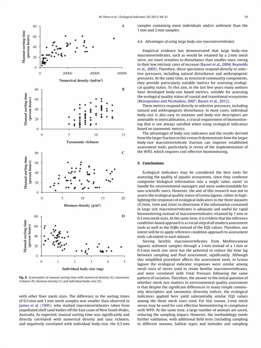
M. Pinna et al. / Ecological Indi
0
20
40
60
80
0 2000 0 4000 0 6000 0
Man
ual s
orti
ng t
ime
(per
son
hour
s)
Numer ical density (ind/m2)
A
0
20
40
60
80
0 5 10 15
Man
ual s
orti
ng t
ime
(per
son
hour
s)
Taxonomic richn ess
B
0
20
40
60
80
0 5 10 15 20
Man
ual s
orti
ng t
ime
(per
son
hour
s)
Biomass density (g/m2)
C
0
20
40
60
80
0 1 2 3 4 5
Man
ual s
orti
ng t
ime
(per
son
hour
s)
Ind ividu al body-size (mg)
D
Fr
woJuAda
with WFD. At the same time, a large number of animals are saved,
ig. 8. Scatterplots of manual sorting time with numerical density (A), taxonomicichness (B), biomass density (C) and individual body-size (D).
ith other finer mesh sizes. The difference in the sorting timesf 0.5 mm and 1 mm mesh samples was smaller than observed inames et al. (1995), who studied macroinvertebrates taken fromnpolluted shelf sand bodies off the East coast of New South Wales,
ustralia. As expected, manual sorting time was significantly andirectly correlated with numerical density and taxa richness,nd negatively correlated with individual body-size, the 0.5 mmcators 29 (2013) 48–61 59
samples containing more individuals and/or sediment than the1 mm and 2 mm samples.
4.4. Advantages of using large body-size macroinvertebrates
Empirical evidence has demonstrated that large body-sizemacroinvertebrates, such as would be retained by a 2 mm meshsieve, are more sensitive to disturbance than smaller ones, owingto their low intrinsic rates of increase (Basset et al., 2004; Reynoldset al., 2005). Therefore, these specimens respond directly to selec-tive pressures, including natural disturbance and anthropogenicpressures. At the same time, as structural community components,they provide particularly suitable metrics for assessing ecologi-cal quality status. To this aim, in the last few years many authorshave developed body-size based metrics, suitable for assessingthe ecological quality status of coastal and transitional ecosystems(Reizopoulou and Nicolaidou, 2007; Basset et al., 2012).
These metrics respond directly to selective pressures, includingnatural and anthropogenic disturbance. In most cases, individualbody-size is also easy to measure and body-size descriptors areamenable to intercalibration, a crucial requirement of biomonitor-ing that is not always satisfied when using ecological indicatorsbased on taxonomic metrics.
The advantages of body-size indicators and the results derivedfrom the larger fraction in this research demonstrate how the largerbody-size macroinvertebrate fraction can improve establishedassessment tools, particularly in terms of the implementation ofthe WFD, which requires cost-effective biomonitoring.
5. Conclusions
Ecological indicators may be considered the best tools forassessing the quality of aquatic ecosystems, since they condensecomposite biological information into a single value, easier tohandle for environmental managers and more understandable fornon-scientific users. However, the aim of this research was not toassess the ecological quality status of Lesina lagoon, rather to high-lighting the responses of ecological indicators in the three datasets(0.5mm, 1mm and 2mm) to determine if the information containedin large size macroinvertebrates is adequate and useful for rapidbiomonitoring instead of macroinvertebrates retained by 1 mm or0.5 mm mesh sizes. At the same time, it is evident that the referencecondition-based approach is a crucial step of all modern assessmenttools as well as the EQRs instead of the EQS values. Therefore, ourintent will be to apply reference condition approach to assessmenttools calculated in each dataset.
Sieving benthic macroinvertebrates from Mediterraneanlagoons sediment samples through a 2 mm instead of a 1 mm or0.5 mm mesh size sieve has the potential to reduce the time lagbetween sampling and final assessment, significantly. Althoughthis simplified procedure affects the assessment tools, in Lesinalagoon the ecological indicator responses were similar amongmesh sizes of sieves used to retain benthic macroinvertebrates,and were correlated with Total Pressure following the samepattern of variation. Therefore, the answer to the initial question ofwhether mesh size matters in environmental quality assessmentis that despite the significant differences in many simple commu-nity descriptors and taxonomic diversity indices, the ecologicalindicators applied here yield substantially similar EQS valuesamong the three mesh sizes used. For this reason, 2 mm meshsieves may be used for cost effective biomonitoring in compliance
reducing the sampling impact. However, the methodology needsfurther validation, with additional field tests (including samplingin different seasons, habitat types and latitudes and sampling
6 al Indi
uoa2sowaem
A
LRtpaewLfi
R
A
A
B
B
B
B
B
B
B
B
B
B
C
C
C
D
0 M. Pinna et al. / Ecologic
nder anthropogenic impacts). Moreover, the reference conditionsf the ecological indicators, especially body-size based ones suchs ISD (Reizopoulou and Nicolaidou, 2007) and ISS (Basset et al.,012), require adjustment. In any case, the reallocation of timeaved by using a 2 mm mesh size sieve would allow samplingf additional replicates, study sites and control sites, or indeedould reduce the time and money required for routine monitoring
ctivities. The process would not only be less expensive, but thexpected outputs would be available to environmental managersore quickly.
cknowledgements
The present study was supported by the WISER project (EU-FP7).aboratory research was carried out in the Experimental Ecologyesearch Centre for Ecosystem Organization, Biodiversity, and Func-ioning of the University of the Salento set up as part of the BIOforIUroject (MIUR – PONa3 00025, 2007–2013). The authors thank twononymous reviewers for their comments and suggestions on anarlier draft. L. Mazzotta, C. Scianna, E. Longo and D. Santagataere involved during field sampling and laboratory analysis. The
esina branch of CNR-ISMAR (Italy) hosted the researcher duringeld activities. G. Metcalf revised the English text.
eferences
guiar, F.C., Feio, M.J., Ferreira, M.T., 2011. Choosing the best method for streambioassessment using macrophyte communities: indices and predictive models.Ecol. Indic. 11, 379–388.
ubry, A., Elliott, M., 2006. The use of environmental integrative indicators to assessseabed disturbance in estuaries and coasts: application to the Humber Estuary,UK. Mar. Pollut. Bull. 53, 175–185.
achelet, G., 1990. The choice of a sieving mesh size in the quantitative assessment ofmarine macrobenthos: a necessary compromise between aims and constraints.Mar. Environ. Res. 30, 21–35.
arba, B., Larranaga, A., Otermin, A., Basaguren, A., Pozo, J., 2010. The effect of sievemesh size on the description of macroinvertebrate. Limnetica 29, 211–220.
asset, A., Sangiorgio, F., Pinna, M., 2004. Monitoring with benthic macroinverte-brates: advantages and disadvantages of body size descriptors. Aquat. Conserv.:Mar. Freshwat. Ecosyst. 14, 43–58.
asset, A., Sabetta, L., Sangiorgio, F., Pinna, M., Migoni, D., Fanizzi, F., Barbone,E., Galuppo, N., Umani, S.F., Reizopoulou, S., Nicolaidou, A., Arvanitidis, C.,Moncheva, S., Trajanova, A., Georgescu, L., Beqiraj, S., 2008. Biodiversity con-servation in Mediterranean and Black Sea lagoons: a trait-oriented approachto benthic invertebrate guilds. Aquat. Conserv.: Mar. Freshwat. Ecosyst. 18 (1),4–15.
asset, A., Barbone, E., Borja, A., Brucet-Balmana, S., Pinna, M., Quintana, X.,Reizopoulou, S., Rosati, I., Simboura, N., 2012. A size spectra index for the WFDimplementation in transitional waters of Mediterranean and Black Sea ecore-gions. Ecol. Indic. 12, 72–83.
attle, J., Jackson, J.K., Sweeney, B.W., 2007. Mesh size affects macroinvertebratedescriptions in large rivers: examples from the Savannah and Mississippi Rivers.Hydrobiologia 592, 329–343.
ishop, J.D.D., Hartley, J.P., 1986. A comparison of the fauna retained on 0.5 and1.0 mm meshes from benthic samples taken in the Beatrice Oilfield, Moray Firth,Scotland. Proc. Roy. Soc. Edinb. 91B, 247–262.
orja, A., Franco, J., Pérez, V., 2000. A marine biotic index to establish the eco-logical quality of soft-bottom benthos within European estuarine and coastalenvironments. Mar. Pollut. Bull. 40, 1100–1114.
orja, A., Miles, A., Occhipinti-Ambrogi, A., Berg, T., 2009. Current status of macroin-vertebrate methods used for assessing the quality of European marine waters:implementing the Water Framework Directive. Hydrobiologia 633, 181–196.
orja, A., Barbone, E., Basset, A., Borgersen, G., Brkljacic, M., Elliott, M., Garmen-dia, J.M., Marques, J.C., Mazik, K., Muxika, I., Neto, J.M., Norling, K., Rodríguez,J.G., Rosati, I., Rygg, B., Teixeira, H., Trayanova, A., 2011. Response of single ben-thic metrics and multimetric methods to anthropogenic pressure gradients, infive distinct European coastal and transitional ecosystems. Mar. Pollut. Bull. 62,499–513.
larke, K.R., Warwick, R.M., 1998. A taxonomic distinctness index and its statisticalproperties. J. Appl. Ecol. 35, 523–531.
larke, K.R., Warwick, R.M., 2001. A further biodiversity index applicable to specieslists: variation in taxonomic distinctness. Mar. Ecol. Prog. Ser. 216, 265–278.
outo, T., Patrício, J., Neto, J.M., Ceia, F.R., Franco, J., Marques, J.C., 2010. The influence
of mesh size in environmental quality assessment of estuarine macrobenthiccommunities. Ecol. Indic. 10, 1162–1173.auvin, J.C., Gomez, G.J.L., Salvande, F.M., 2003. Taxonomic sufficiency: an overviewof its use in the monitoring of sublittoral benthic communities after oil spills.Mar. Pollut. Bull. 46, 552–555.
cators 29 (2013) 48–61
De Biasi, A.M., Bianchi, C.N., Morri, C., 2003. Analysis of macrobenthic communitiesat different taxonomic levels: an example from an estuarine environment in theLigurian Sea (NW Mediterranean). Estuar. Coast. Shelf Sci. 58, 99–106.
EC, 2000. Directive 2000/60/EC of the European Parliament and of the Council Estab-lishing a Framework for Community Action in the Field of Water Policy. OJEC L327/1-72, Brussels.
EC, 2008. Commission Decision of 30 October 2008 Establishing, Pursuant to Direc-tive 2000/60/EC of the European Parliament and of the Council, the Values ofthe Member State Monitoring System Classifications as a Result of the Intercal-ibration Exercise. OJEC, Brussels.
Eleftheriou, A., Holme, N.A., 1984. Macrofauna techniques. In: Holme, N.A., McIn-tyre, A.D. (Eds.), Methods for the Study of Marine Benthos. Blackwell ScientificPublications, Oxford, pp. 140–216.
Ferraro, S.P., Cole, F.A., 2004. Optimal benthic macrofaunal sampling protocol fordetecting differences among four habitats in Willapa Bay, Washington, USA.Estuaries 27, 1014–1025.
Ferraro, S.P., Cole, F.A., Deben, W.A., Swartz, R.C., 1989. Power cost efficiency of eightmacrobenthic sampling schemes in Puget Sound, Washington, USA. Can. J. Fish.Aquat. Sci. 46, 2157–2165.
Ferraro, S.P., Swartz, R.C., Cole, F.A., Deben, W.A., 1994. Optimum macrobenthicsampling protocol for detecting pollution impacts in the southern CaliforniaBight. Environ. Monit. Assess. 29, 127–153.
Fonnesu, A., Pinna, M., Basset, A., 2004. Spatial and temporal variations of detri-tus breakdown rates in the River Flumendosa basin (Sardinia, Italy). Int. Rev.Hydrobiol. 89, 443–452.
Gage, J.D., Hughes, D.J., Vecino, J.L.G., 2002. Sieve size influence in estimatingbiomass, abundance and diversity in samples of deep-sea macrobenthos. Mar.Ecol. Prog. Ser. 225, 97–107.
Gessner, M.O., Chauvet, E., 2002. A case for using litter breakdown to assess func-tional stream integrity. Ecol. Appl. 12, 498–510.
Giordani, G., Zaldivar, J.M., Viaroli, P., 2009. Simple tools for assessing water qualityand trophic status in transitional water ecosystems. Ecol. Indic. 9, 982–991.
Growns, J.E., Chessman, B.C., Jackson, J.E., Ross, G.D., 1997. Rapid assessment ofAustralian rivers using macroinvertebrates: cost and efficiency of 6 methodsof sample processing. J. N. Am. Benthol. Soc. 16, 682–693.
Gruenert, U., Carr, G., Morin, A., 2007. Reducing the cost of benthic sample processingby using sieve retention probability models. Hydrobiologia 589, 79–90.
Hartley, J.P., 1982. Methods for monitoring offshore macrobenthos. Mar. Pollut. Bull.13, 150–154.
ICRAM (Istituto Centrale per la Ricerca Scientifica e Tecnologia Applicata al Mare),2008. Protocolli per il campionamento e la determinazione degli elementi diqualità biologica e fisico-chimica nell’ambito dei programmi di monitoraggio ex2000/60/CE delle acque di transizione. ICRAM, Roma, Italy.
ISO (International Organization for Standardization), 2005. Water Quality – Guide-lines for Quantitative Sampling and Sample Processing of Marine Soft-bottomMacrofauna. ISO, Geneva, Switzerland - EN 16665 2005.
Italian Environmental Ministry, 2008. Criteri tecnici per la caratterizzazione deicorpi idrici, attuazione articolo 75, Dlgs 152/2006. DM 131, GU 187, 11 Agosto2008.
James, R.J., Lincoln Smith, M.P., Fairweather, P.G., 1995. Sieve mesh-size and tax-onomic resolution needed to describe natural spatial variation of marinemacrofauna. Mar. Ecol. Prog. Ser. 118, 187–198.
Kennedy, R., Arthur, W., Keegan, B.F., 2011. Long-term trends in benthic habitat qual-ity as determined by Multivariate AMBI and Infaunal Quality Index in relation tonatural variability: a case study in Kinsale Harbour, south coast of Ireland. Mar.Pollut. Bull. 62, 1427–1436.
Kingston, P.F., Riddle, M.J., 1989. Cost effectiveness of benthic faunal monitoring.Mar. Pollut. Bull. 20, 490–496.
Lampadariou, N., Karakassis, I., Pearson, T.H., 2005. Cost/benefit analysis of a benthicmonitoring programme of organic benthic enrichment using different samplingand analysis methods. Mar. Pollut. Bull. 50, 1606–1618.
Logez, M., Pont, D., 2011. Development of metrics based on fish body size and speciestraits to assess European coldwater streams. Ecol. Indic. 11, 1204–1215.
Macdonald, T.A., Burd, B.J., Macdonald, V.I., Van Roodselaar, A., 2010. Taxonomic andFeeding Guild Classification for the Marine Benthic Macroinvertebrates of theStrait of Georgia, British Columbia. Canadian Technical Report of Fisheries andAquatic Sciences 2874. Canada.
Mancinelli, G., Rossi, L., 2001. Indirect, size-dipendent effects of crustacean meso-grazers on the Rhodophyta Gracilaria verrucosa (Hudson) Papenfuss: evidencefrom a short-term study in the Lesina lagoon (Italy). Mar. Biol. 138, 1163–1173.
Manini, E., Fiordelmondo, C., Gambi, C., Pusceddu, A., Danovaro, R., 2003. Benthicmicrobial loop functioning in coastal lagoons: a comparative approach. Oceanol.Acta 26, 27–38.
Manini, E., Breber, P., D’Adamo, R., Spagnoli, F., Danovaro, R., 2005. Lagoon ofLesina. In: Giordani, G., Viaroli, P., Swaney, D.P., Murray, C.N., Zaldıvar, J.M.,Marshall Crossland, J.I. (Eds.), Nutrient Fluxes in Transitional Zones of theItalian Coast. LOICZ Reports & Studies No. 28. LOICZ, Texel, The Netherlands,pp. 49–54.
Margalef, R., 1969. Perspectives in Ecological Theory. The University of Chicago Press,Chicago.
Marques, J.C., Salas, F., Patrício, J., Teixeira, H., Neto, J.M., 2009. Ecological Indicators
for Coastal and Estuarine Environmental Assessment: A User Guide. WIT Press,UK.Mejer, H., Jørgensen, S.E., 1979. Exergy and ecological buffer capacity. In: Jørgensen,S.E. (Ed.), State of the Art in Ecological Modelling. Copenhagen and PergamonPress, Oxford, pp. 829–846.
al Indi
M
M
M
M
M
M
M
O
P
P
P
P
P
P
P
P
P
P
quality index. Environmetrics 9, 329–357.
M. Pinna et al. / Ecologic
etzeling, L., Chessman, B.C., Hardwick, R., Wong, V., 2003. Rapid assessment ofrivers using macroinvertebrates: the role of experience, and comparisons withquantitative methods. Hydrobiologia 510, 39–52.
istri, M., Munari, C., 2008. BITS: a SMART indicator for soft-bottom, non-tidallagoons. Mar. Pollut. Bull. 56, 580–606.
orin, A., Stephenson, J., Strike, J., 2004. Sieve retention probabilities of streambenthic invertebrates. J. N. Am. Benthol. Soc. 23, 383–391.
ouillot, D., Spatharis, S., Reizopoulou, S., Laugier, T., Sabetta, L., Basset, A., DoChi, T., 2006. Alternatives to taxonomic-based approaches to assess changesin transitional water communities. Aquat. Conserv.: Mar. Freshwat. Ecosyst. 16,469–482.
unari, C., Mistri, M., 2010. Towards the application of the Water FrameworkDirective in Italy: assessing the potential of benthic tools in Adriatic coastaltransitional ecosystems. Mar. Pollut. Bull. 60, 1040–1050.
unari, C., Warwick, R.M., Mistri, M., 2009. Monitoring with benthic fauna in Italiancoastal lagoons: new tools for new prospects. Aquat. Conserv.: Mar. Freshwat.Ecosyst. 19, 575–587.
uxika, I., Borja, A., Bald, J., 2007. Using historical data, expert judgment and multi-variate analysis in assessing reference conditions and benthic ecological status,according to the European Water Framework Directive. Mar. Pollut. Bull. 55,16–29.
rfanidis, S., Pinna, M., Sabetta, L., Stamatis, N., Nakou, K., 2008. Variation of struc-tural and functional metrics in macrophyte communities within two habitatsof eastern Mediterranean coastal lagoons: natural versus human effects. Aquat.Conserv.: Mar. Freshwat. Ecosyst. 18, 45–61.
earson, T., Rosenberg, R., 1978. Macrobenthic succession in relation to organicenrichment and pollution of the marine environment. Oceanogr. Mar. Biol. Annu.Rev. 16, 229–311.
etchey, O.L., Belgrano, A., 2010. Body-size distributions and size-spectra: universalindicators of ecological status? Biol. Lett. 6, 434–437.
ielou, E.C., 1969. An Introduction to Mathematical Ecology. Wiley-Interscience,New York.
inna, M., Basset, A., 2004. Summer drought disturbance on plant detritus decompo-sition processes in three River Tirso (Sardinia, Italy) sub-basins. Hydrobiologia522, 311–319.
inna, M., Sangiorgio, F., Fonnesu, A., Basset, A., 2003. Spatial analysis of plant detri-tus processing in a Mediterranean River type: the case of the River Tirso Basin,Sardinia, Italy. J. Environ. Sci. 15, 227–240.
inna, M., Fonnesu, A., Sangiorgio, F., Basset, A., 2004. Influence of summerdrought on spatial patterns of resource availability and detritus processing inMediterranean stream sub-basins (Sardinia, Italy). Int. Rev. Hydrobiol. 89 (5–6),484–499.
into, R., Patrício, J., Baeta, A., Fath, B.D., Neto, J.M., Marques, J.C., 2009. Review andevaluation of estuarine biotic indices to assess benthic condition. Ecol. Indic. 9,1–25.
onti, M., Pinna, M., Basset, A., Moncheva, S., Trayanova, A., Georgescu, L., Beqiraj, S.,Orfanidis, S., Abbiati, M., 2008. Quality assessment of Mediterranean and BlackSea transitional waters: comparing responses of benthic biotic indices. Aquat.Conserv.: Mar. Freshwat. Ecosyst. 18, 62–75.
onti, M., Vadrucci, M.R., Orfanidis, S., Pinna, M., 2009. Biotic indices for ecological
status of transitional water ecosystems. Transit. Wat. Bull. 3 (3), 32–90.uglia Regional Administration (Regione Puglia, Italia), 2010. La caratterizzazionedei corpi idrici superficiali della Regione Puglia: tipizzazione, identificazione eclassificazione dei corpi idrici. Attuazione DM n. 131 del 16 giugno 2008 (WaterProtection Plan). BURP 64, pp. 10976–11007.
cators 29 (2013) 48–61 61
Reizopoulou, S., Nicolaidou, A., 2007. Index of size distribution (ISD): amethod of quality assessment for coastal lagoons. Hydrobiologia 577,141–149.
Resh, V.H., Jackson, J.K., 1993. Rapid Assessment Approaches to Biomoni-toring Using Benthic Macroinvertebrates. Chapman and Hall, New York,USA.
Reynolds, J.D., Dulvy, N.K., Goodwin, N.B., Hutchings, J.A., 2005. Biology of extinctionrisk in marine fishes. Proc. Roy. Soc. B 272, 2337–2344.
Rhoads, D.C., McCall, P.L., Yingst, J.Y., 1978. Disturbance and production on the estu-arine seafloor. Am. J. Sci. 66, 577–586.
Rodrigues, A.M., Meireles, S., Pereira, T., Quintino, V., 2007. Spatial heterogeneityrecognition in estuarine intertidal benthic macrofaunal communities: influenceof sieve mesh-size and sampling depth. Hydrobiologia 587, 37–50.
Rosenberg, D.M., Resh, V.H., 1993. Introduction to freshwater biomonitoring andbenthic macroinvertebrates. In: Rosenberg, D.M., Resh, V.H. (Eds.), FreshwaterBiomonitoring and Benthic Macroinvertebrates. Chapmann & Hall, New York,pp. 1–9.
Sangiorgio, F., Fonnesu, A., Pinna, M., Sabetta, L., Basset, A., 2006. Influence of droughtand abiotic factors on Phragmites australis leaf decomposition in the River Pula,Sardinia, Italy. J. Freshwat. Ecol. 21 (3), 411–420.
Sangiorgio, F., Basset, A., Pinna, M., Sabetta, L., Abbiati, M., Ponti, M., Minocci, M.,Orfanidis, S., Nicolaidou, A., Moncheva, S., Trayanova, A., Georgescu, L., Dra-gan, S., Beqiraj, S., Koutsoubas, D., Evagelopoulos, A.A., Reizopoulou, S., 2008.Environmental factors affecting Phragmites australis litter decomposition inMediterranean and Black Sea transitional waters. Aquat. Conserv.: Mar. Fresh-wat. Ecosyst. 18, 16–26.
Shannon, C.E., Weaver, W., 1963. The Mathematical Theory of Communication. Uni-versity of Illinois Press, Urbana, Illinois.
Silow, E.A., In-Hye, O., 2004. Aquatic ecosystem assessment using exergy. Ecol. Indic.4, 189–198.
Simboura, N., Zenetos, A., 2002. Benthic indicators to use in Ecological Quality clas-sification of Mediterranean soft bottom marine ecosystems, including a newBiotic Index. Mediterr. Mar. Sci. 3, 77–111.
Specchiulli, A., D’Adamo, R., Renzi, M., Vignes, F., Fabbrocini, A., Scirocco, T., Cilenti,L., Florio, M., Breber, P., Basset, A., 2009. Fluctuations of physicochemical charac-teristics in sediments and overlying water during an anoxic event: a case studyfrom Lesina lagoon (SE Italy). Transit. Wat. Bull. 3 (2), 15–32.
Thompson, B.W., Riddle, M.J., Stark, J.S., 2003. Cost-efficient methods for marinepollution monitoring at Casey Station, East Antarctica: the choice of sieve mesh-size and taxonomic resolution. Mar. Pollut. Bull. 46, 232–243.
Vignes, F., Barbone, E., Breber, P., D’Adamo, R., Roselli, L., Ungaro, N., Focardi, S., Renzi,M., Basset, A., 2009. Spatial and temporal description of the dystrophic crisis inLesina lagoon during summer 2008. Transit. Wat. Bull. 3 (2), 47–62.
Vignes, F., Fedele, M., Pinna, M., Mancinelli, G., Basset, A., 2012. Variability of Lekane-sphaera monodi metabolic rates with habitat trophic status. Acta Oecol. 41,58–64.
Vollenweider, R.A., Giovanardi, F., Montanari, G., Rinaldi, A., 1998. Characterizationof the trophic conditions of marine coastal waters with special reference to theNW Adriatic Sea: proposal for a trophic scale, turbidity and generalized water
Warwick, R.M., 1993. Environmental impact studies on marine communities: prag-matical considerations. Aust. J. Ecol. 18, 63–80.
Zuur, A.F., Ieno, E.N., Elphick, C.S., 2010. A protocol for data exploration to avoidcommon statistical problems. Methods Ecol. Evol. 1, 3–14.
Copyright © 2022 FDOKUMEN