COMPARISON BETWEEN DIFFERENT MODELLING APPROACHES FOR

COASTAL LAGOONS

Annie Chapelle1, Pedro Duarte2, Miguel Angel Esteve3, Annie Fiandrino1, Lorenzo Galbiati4, Dimitar Marinov4, Julia Martinez3, Alain Norro5, Martin Plus1, Christian Salles6, Francesca Somma4, Marie-George

Tournoud6, George Tsirtsis7, José-Manuel Zaldívar4

1 Ifremer, France 2 Centre for Modelling and Analysis of Environmental Systems, Fernando Pessoa

University, Portugal 3 Department of Ecology and Hydrology, University of Murcia, Murcia, Spain 4 European Commission, Joint Research Centre, Institute for Environment and

Sustainability, Ispra, Italy 5 Management Unit of the North Sea, Royal Belgian Institute for Natural Sciences,

Brussels, Belgium 6 Maison des Sciences de l'EAU, Hydrosciences (UMII/CNRS/IRD), Montpellier, France 7 School of Environmental Sciences, Department of Marine Sciences, Aegean

University, Mytilini, Greece

2005 EUR 21817 EN

DITTY PROJECT (Development of an information technology tool for the management

of Southern European lagoons under the influence of river-basin runoff)

D15. COMPARISON BETWEEN DIFFERENT MODELLING APPROACHES FOR COASTAL LAGOONS

(European Commission FP5 EESD Project EVK3-CT-2002-00084)

Annie Chapelle1, Pedro Duarte2, Miguel Angel Esteve3, Annie Fiandrino1, Lorenzo Galbiati4, Dimitar Marinov4,

Julia Martinez3, Alain Norro5, Martin Plus1, Christian Salles6, Francesca Somma4, Marie-George Tournoud6,

George Tsirtsis7, José-Manuel Zaldívar4

1 Ifremer, France 2 Centre for Modelling and Analysis of Environmental Systems, Fernando Pessoa University,

Portugal 3 Department of Ecology and Hydrology, University of Murcia, Murcia, Spain 4 European Commission, Joint Research Centre, Institute for Environment and Sustainability,

Ispra, Italy 5 Management Unit of the North Sea, Royal Belgian Institute for Natural Sciences, Brussels,

Belgium 6 Maison des Sciences de l'EAU, Hydrosciences (UMII/CNRS/IRD), Montpellier, France 7 School of Environmental Sciences, Department of Marine Sciences, Aegean University,

Mytilini, Greece

2005 EUR 21817 EN

LEGAL NOTICE

Neither the European Commission nor any person

acting on behalf of the Commission is responsible for

the use which might be made of the following information.

A great deal of additional information on the

European Union is available on the Internet.

It can be accessed through the Europa server

(http://europa.eu.int)

EUR 21817 EN

© European Communities, 2005

Reproduction is authorised provided the source is acknowledged

Printed in Italy

i

CONTENTS 1. INTRODUCTION 1 2. WATERSHED MODELLING 3

2.1. Presentation of the tools employed 4 2.1.1. SWAT 4 2.1.2. POL 8 2.1.3. AGWFL 10 2.1.4. MODFLOW with MT3DMS 12 2.1.5. QUAL2E 16 2.1.6. MTGera 18 2.1.7. MMHydrological 20 2.1.8. MMWatershed 22 2.1.9. ISSM 25

2.2. Summarizing tables 27 2.3. Model intercomparison analysis 32

3. HYDRODINAMIC MODELLING 35 3.1. Presentation of the tools employed 36

3.1.1. COHERENS 36 3.1.2. POM 36 3.1.3. MARS3D 37 3.1.4. RF2D Hydrodynamics-EcoDynamo 38

3.2. Summarizing tables 41 3.3. Model intercomparison analysis 45

4. BIOGEOCHEMICAL MODELLING 47 4.1. Presentation of the tools employed 48

4.1.1. RF2D Biochemistry-EcoDynamo 48 4.1.2. Mar Menor 52 4.1.3. Etang de Thau 55 4.1.4. Sacca di Goro 58 4.1.5. Gera 60

4.2. Summarizing tables 62 4.3. Model intercomparison analysis 68

5. CONCLUSIONS 70 6. REFERENCES 71

ii

1

1. INTRODUCTION To promote reliable, real-time management of coastal lagoons, increasingly sophisticated numerical models have been developed within the DITTY project (WP4). While models are diverse in design and scope, i.e. watershed, fluid-dynamics, biogeochemical, all have the same fundamental goal, i.e. to account realistically for the processes that drive the dynamic behaviour in coastal lagoons so that their status may ultimately be predicted and the effects of mitigation actions be properly evaluated, resulting on a series of good management practices that increase the sustainability of these fragile ecosystems. The intent, which is also the final goal of D16, is to establish a standard set of input parameters and numerical “experiments” to be performed by various existing models so that independent results could be meaningfully compared and evaluated, having in mind the diversity of approach and systems (watershed, lagoon, adjacent coastal area). Furthermore, though comparison, conceptual weakness could be identified and targeted for further exploration by the DITTY partners as a whole. In this Deliverable a first attempt to describe, summarise and analyse the used models have been made. Model intercomparison techniques have been developing over the years in a number of environmental research communities (Røed et al., 1995; Hackett et al., 1995; Proctor, 1997 and 2002; Cramer and Field, 1999; Denning et al., 1999; Orr, 1999; Skogen and Moll, 2000; Beckers et al., 2002; Davies et al., 2002; Caputo et al., 2003; Smith et al., 2004; Delhez et al., 2004). For example, Smith et al. (2002) developed a distributed model intercomparison project (DMIP) to compare simulation of distributed hydrologic models to investigate several issues, such as: nature and impact of spatial variability of basin physical characteristics and forcings, optimal level of basin disaggregation to captures essential spatial variability, nature of error propagation through distributed models. Concerning hydrodynamic models, Beckers et al. (2002) carried out an intercomparison exercise on several water circulation models applied to the Mediterranean Sea using the same forcing. The results show that no model performed better than the others and that there was a similar correlation between model characteristics and modeller’s skill in terms of results. Intercomparison analysis concerning biogeochemical models are more scarce, for example a limited exercise was carried out by Skogen and Moll (2000) concerning the primary production of the North Sea using two ecological models. Both models gave similar results on the annual mean primary production, its variability and the influence of the river inputs. As already stated, the goals of an intercomparison exercise are always the same. However, the processes we are interested in assess through the developed models are quite different and the requests in terms of data input, forcing variables, validation data, as well as calibration and sensitivity analysis are not completely similar. As we are concerned with three fundamentally different realms of modelling (watershed, hydrodynamic, biogeochemical modelling), we have decided to structure the document in three separate sections. The analysis will serve as a preliminary screening mechanism to select which techniques/tools can (realistically) be implemented in the Decision Support System (DSS). Furthermore, it has the objective of assessing the confidence in the model outputs/predictions from the defined scenario analysis which in turn will support

2

decision making in coastal lagoons. The final outcome of the analysis will be a guide for coastal lagoon modellers that may help the implementation of similar tools to other coastal lagoons.

3

2. WATERSHED MODELLING Watershed modelling refers to a class of tools able to describe the movement of water in a river basin, both in terms of hydrological cycle and hydraulic routing. Often times such models, other than the movement of water, include the transport of constituents, thus accounting for their decay, precipitation, dissolving, dispersion and chemical reactions, all changing the concentration of the constituents as water flows along. Many of them can realistically account for detailed watershed morphology; land use and land cover distribution; point sources and water protection/water management infrastructures (levees, canals, artificial impoundments, etc.). Simulation models are used extensively in water quantity and quality planning and pollution control, and are applied to answer a variety of questions: provide real-time hydrologic forecasting, support watershed analysis and planning, develop total maximum daily loads (TMDL). Many models of such type are available in the literature, each of them with a different emphasis, depending on the scope for which it was created. Some models are highly specialized to simulate environmental phenomena and components of pollution problems; others incorporate more comprehensive assessment techniques. For example, there are specialized models to predict localized pollutant transport, at field scale, and comprehensive watershed-scale models that simulate pollutant loading, transport and transformation. Watershed-scale models can be classified according to a number of classification criteria. For example, EPA (1997) distinguishes three major categories of models: watershed loading, receiving water and ecological models. In particular, the first ones simulate the generation and movement of pollutants from land surface (point or diffuse source) to water bodies, while the second and third ones deal with movement and transformation within a water body (lakes, estuaries, coastal waters), including eutrophication and simulation of biological communities, respectively. Other types of classifications relate to: - the temporal scale dealt by the model (event based versus annual or continuous); - the approach used to describe the various processes (empirical, physically based); - the spatial scale (lumped, where the watershed is treated as a box with input and

output, versus distributed, were transport is simulated taking into account the spatial variability of the physical characteristics of the watershed and its land cover).

Moreover, depending on the level of complexity, some of such models are actually “super-models”, or integrated models, linking several models together, each describing fully only one of the processes contributing to transport. Following the increasing computing capabilities and the mounting wealth of data collected though the monitoring networks, along with the recent development of geographic information system (GIS) tools, researchers have poured considerable effort into developing distributed models. Such class of model is more apt to the exploration of research oriented issues and to detailed description of the movement of pollutants and the effects of land use change. However, with computational and modelling advances, a new realm of questions has raised to prominence. For example, as complexity in modelling represents a cost, in terms of data requirement, model calibration and validation, and computational effort, an important issue of discussion is the definition of the level of complexity necessary to achieve the desired accuracy in process simulation. Other questions relate to the impact of spatial variability of basin physical

4

characteristics and forcings, dominancy and representativeness of scales to parametric uncertainty, error propagation though the models, and last but not least, calibration at the watershed outlet and, where necessary, at interior points. Several studies have been reported in the literature as trying to shed some light on these issues (see references in Smith et al., 2004). However, often times the focus was on model performance (one model being applied to several basins) rather that basin response. A distributed model intercomparison project (DMIP) has been set up (Smith et al., 2004) as a broad base for comparison of distributed models against a lumped model used for operational river forecasting in US. Project participants applied a variety of models, ranging from complex, physically based distributed models to sub-basin approaches using lumped conceptual models, to three selected US watersheds. One of the aims of DMIP researchers was to assess the sensitivity of the models to spatial and temporal variability of rainfall. In particular, research evidence prior to the start of the DMIP, hinted to the possibility of improving lumped hydrological models by using semi-distributed or distributed modelling approaches using the so-called physically based or conceptual rainfall-runoff mechanisms. Other questions addresses regarded the capability of identifying which basins would benefit from distributed versus lumped models, to which extent it was beneficial to increase complexity of the model itself, and to what extent to increase the level of effort required for model calibration. Results from the project are not entirely conclusive due to restricted number of test locations; however, preliminary findings suggest, for example, that distributed models will over lumped models when there is the necessity of producing accurate estimates at un-gauged locations. Spatial and temporal scales at which distributed models can give more accurate results than lumped model is still not clear. Within the Ditty project several modelling approaches were tested at the various study sites. The characteristics of these models (conceptual approach, space and time scale, data requirements, output characteristics) will be illustrated in the following paragraphs, and similarities and diversities highlighted. The adaptability of each model as a tool integrated within a decision support system will also be commented upon. 2.1. Presentation of the tools employed 2.1.1. SWAT Introduction/Brief description. The model SWAT - Soil and Water Assessment Tool - is a fully distributed, physically based, three-dimensional, continuous time watershed model that operates on a daily time step at watershed scale. The major objective of the model is to predict the long-term impacts in large basins of management and also timing of agricultural practices within a year (i.e., crop rotations, planting and harvest dates, irrigation, fertiliser, and pesticide application rates and timing). It can be used to simulate water and nutrient cycles at the basin scale in landscapes where the dominant land use is agriculture. It can also help in assessing the environmental efficiency of best management practices and alternative management policies. The chemicals considered in the model include nutrients (N-based, P-based, O-based and algae) and pesticides. The model is not designed to simulate detailed, single-event flood routing. A complete description of the theory behind the SWAT model can be found in Neitsch et al. (2002a).

5

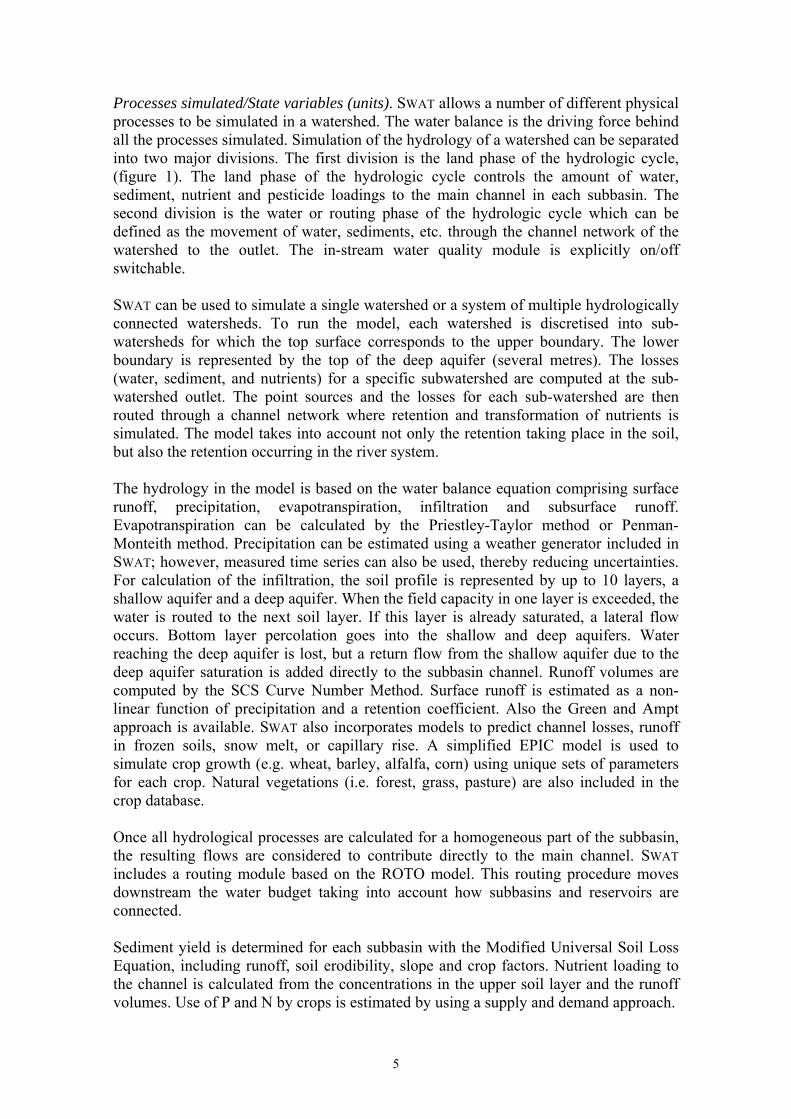
Processes simulated/State variables (units). SWAT allows a number of different physical processes to be simulated in a watershed. The water balance is the driving force behind all the processes simulated. Simulation of the hydrology of a watershed can be separated into two major divisions. The first division is the land phase of the hydrologic cycle, (figure 1). The land phase of the hydrologic cycle controls the amount of water, sediment, nutrient and pesticide loadings to the main channel in each subbasin. The second division is the water or routing phase of the hydrologic cycle which can be defined as the movement of water, sediments, etc. through the channel network of the watershed to the outlet. The in-stream water quality module is explicitly on/off switchable. SWAT can be used to simulate a single watershed or a system of multiple hydrologically connected watersheds. To run the model, each watershed is discretised into sub-watersheds for which the top surface corresponds to the upper boundary. The lower boundary is represented by the top of the deep aquifer (several metres). The losses (water, sediment, and nutrients) for a specific subwatershed are computed at the sub-watershed outlet. The point sources and the losses for each sub-watershed are then routed through a channel network where retention and transformation of nutrients is simulated. The model takes into account not only the retention taking place in the soil, but also the retention occurring in the river system. The hydrology in the model is based on the water balance equation comprising surface runoff, precipitation, evapotranspiration, infiltration and subsurface runoff. Evapotranspiration can be calculated by the Priestley-Taylor method or Penman-Monteith method. Precipitation can be estimated using a weather generator included in SWAT; however, measured time series can also be used, thereby reducing uncertainties. For calculation of the infiltration, the soil profile is represented by up to 10 layers, a shallow aquifer and a deep aquifer. When the field capacity in one layer is exceeded, the water is routed to the next soil layer. If this layer is already saturated, a lateral flow occurs. Bottom layer percolation goes into the shallow and deep aquifers. Water reaching the deep aquifer is lost, but a return flow from the shallow aquifer due to the deep aquifer saturation is added directly to the subbasin channel. Runoff volumes are computed by the SCS Curve Number Method. Surface runoff is estimated as a non-linear function of precipitation and a retention coefficient. Also the Green and Ampt approach is available. SWAT also incorporates models to predict channel losses, runoff in frozen soils, snow melt, or capillary rise. A simplified EPIC model is used to simulate crop growth (e.g. wheat, barley, alfalfa, corn) using unique sets of parameters for each crop. Natural vegetations (i.e. forest, grass, pasture) are also included in the crop database. Once all hydrological processes are calculated for a homogeneous part of the subbasin, the resulting flows are considered to contribute directly to the main channel. SWAT includes a routing module based on the ROTO model. This routing procedure moves downstream the water budget taking into account how subbasins and reservoirs are connected. Sediment yield is determined for each subbasin with the Modified Universal Soil Loss Equation, including runoff, soil erodibility, slope and crop factors. Nutrient loading to the channel is calculated from the concentrations in the upper soil layer and the runoff volumes. Use of P and N by crops is estimated by using a supply and demand approach.

6

Figure 1. Hydrologic cycle components developed in SWAT (from Neitsch et al., 2002b). The nitrogen module also includes processes like mineralization, denitrification, and volatilisation. Phosphorus association with the sediment phase is also considered in the phosphorus module. Both modules are based on the CREAMS model. After considering the N and P dynamics (see figure 2), the chemicals are also routed into the subbasin channels. Main state variable for SWAT can be considered the soil moisture. All variables are expressed in SI units. A complete list of variables (meteo, soil, crop, etc) and units can be found in the SWAT user manual Neitsch et al. (2002b). Input requirements/Data preprocessing. SWAT is a comprehensive model that requires a diversity of information in order to run. As a rough estimate, 3-4 months are requested to setup the necessary databases (starting from available data) and run, calibrate and validate the model. It is important to run the model for a number of years before the period of interest, for model processes “warm-up”. Basic GIS/ArcView knowledge is also required to set up the relevant ArcView map themes and data files in the model. Minimum input requirements (to generate simulated flow series) are: a DEM of the studied area; meteorological station coverage; meteorological series at one or more stations representative of the area of interest (SWAT has a weather generator for the calculation of missing data or to generate meteorological series); soil properties; land use/cover; agricultural management practices. Additional input (fertilizer/pesticide application schedule, point source, reservoir information, etc.) is required only on a case to case basis (again see Neitsch et al., 2002b). After having appropriately prepared the required input files, all in dbf format, preprocessing through the ArcView interface results in the identification of all parcels with unique soil/land use combination (hydrologic response unit, HRU) and the compilation of the input files actually used by the model.

7

Figure 2. Partitioning of Nitrogen and Phosphorus in SWAT (from Neitsch et al., 2002b). Output/postprocessing/scenario analysis. Output from SWAT is very involved and results in a large number of files, where variables are aggregated at different levels (HRU, subbasin, basin). Some general, synthetic output is generated at watershed level in terms of water flow, sediment, nutrient, and pesticide loads at the watershed outlet. All time dependent output is generated at daily scale. No sub-daily output is generated, as SWAT does not deal with event based simulations. All output is expressed in SI units. For a comprehensive description of output consult Neitsch et al. (2002b). SWAT is a river basin, or catchment scale model developed to predict the impact of land management practices on water, sediment and agricultural chemical yields in large, complex catchments with varying soils, land use and management conditions over long periods of time. Different scenarios can refer to changing climate, land use, agricultural management, water management and structural BMP implementation. The model is physically based and computationally efficient, uses readily available inputs and enables the users to study long term impacts. Limits of application. Some hidden bugs in the interface however, require some experience or the assistance of experienced users. Also the interface relays heavily on dbf files that are easily corrupted by Microsoft Excel. Accessibility/Portability/Manuals/References. SWAT is a public domain model developed by the USDA Agricultural Research Service at the Grassland, Soil and Water Research Laboratory in Temple, Texas, USA. SWAT code is available, free of charge, at the following website: http://www.brc.tamus.edu/swat/soft_model.html. The model can be run “as is” on PC (DOS/Windows) and Unix (Solaris) environments. However, a GIS interface is available for easy handling of spatial input and output. AVSWAT (ArcView SWAT) is a complete preprocessor, interface and post processor of the

8

hydrological model SWAT providing the user with a complete set of tools for the watershed delineation, definition and editing of the hydrological and agricultural management inputs, running and calibration of the model. The extension and the model constitute a comprehensive and user friendly tool for the watershed scale assessment and control of the agricultural and urban sources of water pollution. SWAT theory and user manuals have been referenced in the previous paragraphs. 2.1.2. POL Introduction/Brief description. The water quality model POL has been especially developed for small Mediterranean catchments (Payraudeau et al., 2004). This model simulates directly pollutant loads produced during flood events: it does not run separately flows and concentrations. The model is able to simulate dissolved nitrogen and phosphorus loads. It follows a simple conceptual semi-distributed approach. The POL model is an event-based model: it runs on an hourly time step. The catchment is delineated into hydrological units (sub-catchments and river-reaches) for which geomorphologic characteristics (area, slopes, length) and land use properties are defined. So the model permits to consider the spatial variability of human activities. DEM data, land use map, agricultural practices, pollutant point sources (such as location of sewage treatment plants) are required. Pollutant point sources are defined as direct inputs in the river. First the river network is divided into river reaches according to point source and main tributaries locations. Then the catchment is delineated into hydrological units (Rodriguez-Iturbe and Gupta, 1983), according to the topography. For each unit (sub-catchment or river reach), geomorphologic characteristics (area, slopes, length) and land use properties are processed (Payraudeau et al., 2001). Two processes are considered in the model: (i) the production of dissolved pollutant loads by the hydrological units during the rainfall event and (ii) the routing of these loads along the river reaches. Two hypotheses are assumed: (i) rainfall drives pollutant mobilisation on the sub-catchment surfaces; (ii) pollutant loads are conservative along the river reaches during the event. The production process on a given sub-catchment is represented by a simple linear reservoir (Figure 4a). At the beginning of the rainfall event, the reservoir content is calculated as a proportion � of the initial pollutant stock N on the whole catchment, which is set by calibration. The proportion � depends on agricultural practises and land uses of the sub catchment related to those of the catchment. The Lag-time of the reservoir is considered as uniform over the catchment. It is related, through a filter function, to the rainfall event in which the coefficient F is the second parameter of the model (Figure 4b).

9

Figure 3. TN flux variables definition.

The routing process along a river reach is represented by a series of linear reservoirs. At the beginning of the rainfall event, the routing reservoirs are all empty. The lag-time T of the river reservoirs is assumed to be uniform over the whole river. It is the third parameter of the model (Figure 4). The number of reservoirs for a given reach depends on its length of the reach. The model has three parameters: one initial value (N), a production parameter (F) and a routing parameter (T). The initial pollutant stock N ranges from 0 to 2; values higher than 2 gave unrealistic loads. Theoretical range of F parameter is from 0 to 1. T parameter ranges from 0 to 4; these values match mean routing velocity around 1 m/s.

Figure 4. Formalization of dissolved nutrients production process.

10

Figure 5. Formalization of dissolved nutrients transport process.

2.1.3. AGWFL Introduction/Brief description. The core watershed simulation model for this GIS-based application is the GWLF (Generalized Watershed Loading Function) model developed by Haith and Shoemaker (1987). GWLF is considered to be a combined distributed/lumped parameter watershed model. For surface loading, it is distributed in the sense that it allows multiple land use/cover scenarios, but each area is assumed to be homogenous in regard to various attributes considered by the model. Additionally, the model does not spatially distribute the source areas, but simply aggregates the loads from each area into a watershed total; thus, no spatial routing is considered. For sub-surface loading, the model acts as a lumped parameter model using a water balance approach. No distinctly separate areas are considered for sub-surface flow contributions. Daily water balances are computed for an unsaturated zone as well as a saturated sub-surface zone, where infiltration is simply computed as the difference between precipitation and snowmelt minus surface runoff plus evapotranspiration. Processes simulated/State variables (units). The GWLF model provides the ability to simulate runoff, sediment, and nutrient (N and P) loadings from a watershed given variable-size source areas (i.e., agricultural, forested, and developed land). It also has algorithms for calculating septic system loads, and allows for the inclusion of point source discharge data. It is a continuous simulation model that uses daily time steps for weather data and water balance calculations. Monthly calculations are made for sediment and nutrient loads, based on the daily water balance accumulated to monthly values. With respect to the major processes simulated, GWLF models surface runoff using the SCS-CN approach with daily weather (temperature and precipitation) inputs. Erosion and sediment yield are estimated using monthly erosion calculations based on the USLE algorithm (with monthly rainfall-runoff coefficients) and a monthly composite of KLSCP values for each source area (i.e., land cover/soil type combination). A sediment delivery ratio based on watershed size, and a transport capacity based on average daily runoff, are then applied to the calculated erosion to determine sediment yield for each source area. Surface nutrient losses are determined by applying dissolved N and P coefficients to surface runoff and a sediment coefficient to

11

the yield portion for each agricultural source area. Point source discharges can also contribute to dissolved losses and are specified in terms of kilograms per month. Manured areas, as well as septic systems, can also be considered. Urban nutrient inputs are all assumed to be solid-phase, and the model uses an exponential accumulation and wash-off function for these loadings. Sub-surface losses are calculated using dissolved N and P coefficients for shallow groundwater contributions to stream nutrient loads, and the sub-surface sub-model only considers a single, lumped-parameter contributing area. Evapotranspiration is determined using daily weather data and a cover factor dependent upon land-use/cover type; the user has the choice of selecting the Hammond or the Blaney-Criddle method for computations. Finally, a water balance is performed daily using supplied or computed precipitation, snowmelt, initial unsaturated zone storage, maximum available zone storage, and evapotranspiration values. In addition to the routines present in the original GWLF, a stream bank erosion routine is implemented in AVGWLF, based on an approach often used in the field of geomorphology in which monthly stream bank erosion is estimated by first calculating a watershed-specific lateral erosion rate using the equation of the form:

LER = aq0.6 (1)

where LER is an estimated lateral erosion rate; a is an empirically-derived constant related to the mass of soil eroded from the stream bank depending upon various watershed conditions, and; q is the monthly stream flow (m3/s). After a value for LER has been computed, the total sediment load generated via stream bank erosion is then calculated by multiplying the above erosion rate by the total length of streams in the watershed (in meters), the average stream bank height (m), and the average soil bulk density (kg/m3). Input requirements/Data preprocessing. For execution, the model requires three separate input files containing transport, nutrient, and weather related data. The transport (TRANSPORT.DAT) file defines the necessary parameters for each source area to be considered (i.e., area size, curve number, etc.) as well as global parameters (i.e., initial storage, sediment delivery ratio, etc.) that apply to all source areas. The nutrient (NUTRIENT.DAT) file specifies the various loading parameters for the different source areas identified (i.e., number of septic systems, urban source area accumulation rates, manure concentrations, etc.). The weather (WEATHER.DAT) file contains daily average temperature and total precipitation values for each year simulated. All such files can be prepared using the ArcView preprocessing interface included in the model. Information for compilation of the necessary input files is derived by both processing all the required GIS layers (DEM, meteorological station location, stream network, soil, land use/cover, point sources, manure, N and P loads, animal density, erodibility, etc.), by automatic loading (rainfall, minimum and maximum temperature series) and by manual input though the interface. Watershed delineation is also achieved through the interface during preprocessing. After being generated the input files can also be manually modified for model calibration and validation. Output / postprocessing / scenario analysis. Typical standard AVGWLF output (precipitation, water flow, sediment load, N and P loads) can be viewed in two formats: average output, comprising a summary of the model output results; monthly results for each individual year simulated. Results can be viewed either in tabular or graphical

12

form. All of the model output, both tabular and graphical, can be printed directly or exported as a JPEG image file. AVGWLF has not built-in scenario analysis, although scenario analysis can be performed by varying the appropriate parameters (land use, agricultural management, point-source load) and comparing output. However, a software application is available for evaluating the implementation of both agricultural and non-agricultural pollution reduction strategies at the watershed level. PRedICT (Pollution Reduction Impact Comparison Tool) allows the user to create various “scenarios” in which current landscape conditions and pollutant loads (both point and non-point) can be compared against “future” conditions that reflect the use of different pollution reduction strategies (best management practices) such as agricultural and urban BMPs, the conversion of septic systems to centralized wastewater treatment, and upgrading of treatment plants from primary to secondary to tertiary. The software includes pollutant reduction coefficients for nitrogen, phosphorus and sediment; cost information for an assortment of BMPs and wastewater upgrades are also built-in. However, it must be noted that most of the BMPs are analyzed through emission reduction coefficient linked to cost functions, rather that though a full simulation. Limits of application. AVGWLF is designed to produce output in SI units, but much of the model is still coded to receive input in English units, thus confusing the user as to how to prepare the appropriate file. This is often times confusing, and thorough check of precipitation and flow output is required to ascertain that variables have been input in the correct units. As most continuous models, AVGWLF requires a period of warm-up before simulation output can be produced without the bias of initial conditions. No single event simulation can be produced. Finally, while the model produces daily water flow output, sediment and nutrient loads are only computed at monthly scale, so that result validation is difficult in those areas where only scattered measurements are available. Accessibility/Portability/Manuals/References. AVGWLF is available free of charge at www.avgwlf.psu.edu. At the same site, user manuals, reference publications and contacts for reference people can be found. Running the model requires the installation of ArcView 3.2. 2.1.4. MODFLOW with MT3DMS Introduction/Brief description. MODFLOW is a program that numerically solves the three-dimensional ground-water flow equation for a porous medium by using a finite-difference method. The code was first published in 1984, and then it has been updated several times with the additions of new capabilities. The latest version of the code is called MODFLOW-2000. The model simulates steady and non-steady flow in an irregularly shaped flow system in which aquifer layers can be confined, unconfined, or a combination of those two typologies and unconfined. Model layers can have varying thickness. The flow region is subdivided into cells in which the medium properties are assumed to be uniform. The Darcy’s law governs the flow rate, which is solved using the finite-difference approximation. For each cells the model calculates the unknown head, referenced to a point allocated at the centroid of the cell itself. Thus, a flow

13

equation is written for each cell. The mathematical solution of the resulting matrix is carried out using the finite-difference method (figure 6). To solve the resulting matrix problem the user can choose the best solver for the particular problem out of the several available in the model. Flow from external stresses, such as flow to wells, areal recharge, evapotranspiration, flow to drains, and flow through river beds, can be simulated. Hydraulic conductivities or transmissivities for any layer may differ spatially and be anisotropic (restricted to having the principal directions aligned with the grid axes), and the storage coefficient may be heterogeneous. Specified head and specified flux boundaries can be simulated as can a head dependent flux across the model's outer boundary that allows water to be supplied to a boundary block in the modelled area at a rate proportional to the current head difference between a "source" of water outside the modelled area and the boundary block. Flow-rate and cumulative-volume balances from each type of inflow and outflow are computed for each time steps.

Figure 6. Example of a finite difference grid used by MODFLOW.

The Finite difference method

In the finite difference method applied to an

aquifer system consist in dividing the

groundwater tables in different layers. Each

layers is then discretised in a grid of

rectangular blocks. The modelled area is

subdivided in cells in which one assumes

that the properties of the aquifer are

uniform. The resulting 3D grid is composed

by cells, group of cells are composing lines

and columns.

Processes simulated/State variables. MODFLOW-2000 has a conceptual-modular structure, which can be summarized in four modularisation entities: packages, procedures, modules and processes. The module is the most fundamental entity. Modules can be grouped according to packages or procedures in order to match the user needs and perspective. Packages take care to simulate each hydrologic capability, such as leakage to rivers, recharge, and evapotranspiration. Procedures are the pieces of the code composing the high-complex MODFLOW programming source code. Each package is composed by a combination of procedures. To make it possible to divide easily the program into both packages and procedures as desired, the program code is broken into smaller pieces called modules. Each module contains the program code within a single procedure for a single package. A process is a part of the code that solves a fundamental equation by a specified numerical method. For example, the solution of the ground-water flow

14

equation using the finite-difference method is called in MODFLOW-2000 Ground-Water Flow (GWF) process. Depending on what processes are included along with the Ground-Water Flow Process, MODFLOW-2000’s structure can be significantly more complex than it was originally designed. For example, when the Observation, Sensitivity, and Parameter-Estimation Processes are added, a new parameter estimation loop is added to the structure, which allows the Ground-Water Flow Process to be executed multiple times, and a new parameter sensitivity loop is added. Due its modular structure, it is not really easy to highlight state variables of MODFLOW-2000. As above mention the number of state variables and the complexity of the simulation is strongly related with the number and/or combination of packages activated by the user during the simulation. For example, the DITTY application of MODFLOW-2000 includes the MT3DMS package. MT3DMS is a modular three-dimensional multi-species transport model for simulation of advection-dispersion and chemical reaction of contaminants in the ground-water system. It uses either mixed Eulerian-Lagrangian approach or the finite difference method to solve the three-dimensional advective-dispersive-reactive equation. MT3DMS uses a modular structure similar to that implemented in MODFLOW 2000. It can be used to simulate changes in concentrations of miscible contaminants in groundwater considering advection, dispersion, diffusion, and some basic chemical reactions, with various types of boundary conditions and external sources or sinks. The chemical reactions included in the model are equilibrium-controlled or rate-limited linear or nonlinear sorption and first-order irreversible or reversible kinetic reactions. It should be noted that the basic chemical reaction package included in MT3DMS is intended for single-species systems. - Governing Equations: The fate and transport of contaminants of species k in 3-D,

transient groundwater flow systems is described by a partial differential equation which takes into account the advection, dispersion, chemical reactions and sorption terms.

- Advection: The advection term of the transport equation describes the transport of miscible contaminants at the same velocity as the groundwater. For many field-scale contaminant transport problems, the advection term dominates over other terms.

- Dispersion: Dispersion in porous media refers to the spreading of contaminants over a greater region than would be predicted solely from the average groundwater velocity vectors. Dispersion is caused by mechanical dispersion, a result of deviations of actual velocity on a microscale from the average groundwater velocity, and by molecular diffusion driven by concentration gradients. Molecular diffusion is generally secondary and negligible, compared with the effects of mechanical dispersion, and only becomes important when groundwater velocity is very low. The sum of mechanical dispersion and molecular diffusion is termed hydrodynamic dispersion, or simply dispersion. Although the dispersion mechanism is generally understood, the representation of dispersion phenomena in a transport model is the subject of intense continuing research.

- Chemical Reactions: The MT3DMS code is capable of handling equilibrium-controlled linear or nonlinear sorption, non-equilibrium (rate-limited) sorption, and first-order reaction that can represent radioactive decay or provide an approximate representation of biodegradation. The general formulation designed to model rate-limited sorption can also be used to model kinetic mass transfer between the mobile

15

and immobile domains in a dual-domain advection-diffusion model. More sophisticated chemical reactions can be modelled through add-on reaction packages.

- Equilibrium-controlled linear or nonlinear sorption: Sorption refers to the mass transfer process between the contaminants dissolved in groundwater (aqueous phase) and the contaminants sorbed on the porous medium (solid phase). It is generally assumed that equilibrium conditions exist between the aqueous-phase and solid-phase concentrations and that the sorption reaction is fast enough, relative to groundwater velocity, to be treated as instantaneous. The functional relationship between the dissolved and sorbed concentrations under a constant temperature is referred to as the sorption isotherm. Equilibrium-controlled sorption isotherms are generally incorporated into the transport model through the use of the retardation factor. Three types of equilibrium-controlled sorption isotherms (linear, Freundlich, and Langmuir) are considered in the MT3DMS transport model. Additional details are given by Zheng et al. (1999). Detailed information about the packages is available in McDonald and Harbaugh (1988) and Harbaugh and McDonald (1996).

Input requirements/Data preprocessing. A large amount of information and a complete description of the flow system are required to make the most efficient use of MODFLOW-2000. In situations where only rough estimates of the flow system are needed, the use of MODFLOW-2000 may not be justified because of the extensive input requirements. To use MODFLOW-2000, the region to be simulated must be divided into cells with a rectilinear grid resulting in layers, rows and columns. Files must then be prepared that contain hydraulic parameters (hydraulic conductivity, transmissivity, specific yield, etc.), boundary conditions (location of impermeable boundaries and constant heads), and stresses (pumping wells, recharge from surface). Several user interfaces are available to assist in setting up input data set, most of which developed in Visual Basic (i.e., GMS - Groundwater Modelling System and Visual MODFLOW). There are also interfaces developed for windows environment, such as PMwin and GIS interfaces. Output/postprocessing/scenario analysis. The MODFLOW-2000 outputs are related with the groundwater trends and the content of water of the cell belonging to the matrix built for the simulation. The model reports the time series only for those cells selected at the beginning of the simulation as calibration cells. This means that if no calibration cells are chosen, no time series on groundwater trends will be available at the end of the simulation. Implementing the Zone Budget packages, MODFLOW-2000 calculates sub-regional water budgets derivate from the finite difference solution of the Darcy law. It uses cell-by-cell flow data saved by the model in order to calculate the budgets. The user assigns a zone number for each cell in the model. Composite zones can also be defined as combinations of the numeric zones. Choosing a stress period (in days) at the beginning of the simulation, the user establishes both the time step for the simulation and the time step for reporting the output. Most common time steps are 30 days or, in case of smaller areas, 5 or 10 days. Due to the high complexity of the calculation carried out by MODFLOW-2000, it is important to highlight that smaller stress period will make the simulation exceedingly time consuming. Limits of application/Accessibility/Portability/Manuals/References. MODFLOW-2000 is most appropriate in those situations requiring the achievement of accurate description of the flow system. MODFLOW-2000 was developed using the finite-difference method.

16

The finite-difference method allows a physical explanation of the concepts used in construction of the model. Therefore, MODFLOW-2000 is easily learned and modified to represent more complex features of the flow system. On the other hand, the set-up of the model is really complex, therefore its use can be very time consuming. Complete documentation, manual and references of MODFLOW-2000 are available under the USGS (U.S. Geological Survey) web site: http://water.usgs.gov/ 2.1.5. QUAL2E Introduction/Brief description. The Enhanced Stream Water Quality Model (QUAL2E) is a comprehensive one-dimensional stream water quality model. It simulates the major reactions of nutrient cycles, algal production, benthic and carbonaceous demand, atmospheric re-aeration and their effects on the dissolved oxygen balance. The model also includes a heat balance for the computation of temperature and mass balances for conservative minerals, Coliform bacteria, and non-conservative constituents such as radioactive substances. QUAL2E has been explicitly developed for steady flow and steady waste-load conditions and is therefore a “steady state model”, although temperature and algae functions can vary on a diurnal basis. The core of the models has been established in 1987 (Brown and Barnwell, 1987). Since then, several interfaces and the integration of the model with other codes (i.e. SWAT) have been developed. Processes simulated/State variables. The conceptual representation of a stream used in the QUAL2E formulation is a stream reach that has been divided into a number of sub-reaches or computational elements equivalent to finite difference elements. For each computational element, a hydrologic balance in terms of flow, a heat balance in terms of temperature, and a materials balance in terms of concentration is written. Both advective and dispersive transports are considered in the materials balance. The model uses a finite-difference solution of the advective-dispersive mass transport and reaction equations and it specifically uses a special steady-state implementation of an implicit backward difference numerical scheme which gives the model an unconditional stability (Walton and Webb, 1994). In each compartment, the model computes the major interactions between up to 15 state variables.

• BOD - Ultimate carbonaceous biochemical oxygen demand (BOD) is modelled as a first-order degradation process in QUAL2E, which also takes into account removal by settling and does not affect the oxygen balance.

• DO - The process discussed above represents the primary internal sink of dissolved oxygen in the QUAL2E computer program. Other sinks include sediment oxygen demand (SOD), modelled as a zero-order reaction, respiration by algae, and nitrification, which includes the oxidation of both ammonia and nitrite. The major source of dissolved oxygen, in addition to that supplied from algal photosynthesis, is atmospheric re-aeration. Nine methods are available to calculate the re-aeration coefficient in case of free water surface. Re-aeration under ice cover and above dams is also considered. All sources and sinks (but SOD) are modelled as first order reactions.

• The nitrogen cycle is composed of four compartments: organic nitrogen, ammonia nitrogen, nitrite nitrogen, and nitrate nitrogen. The nitrogen balance considers mineralization and settling of the organic nitrogen, nitrification which is divided into the oxidation of ammonia in nitrite and then the oxidation of nitrite into

17

nitrate, uptake by the algae, regeneration from the sediment and from algal respiration. Both nitrification reaction rates can be corrected to take into account inhibition at low DO concentrations.

• The phosphorus cycle is similar to, but simpler than the nitrogen cycle, having only two compartments. The phosphorus balance considers the settling and the mineralization of the organic phosphorus into inorganic phosphorus, regeneration from the sediment, uptake and respiration from the algae.

• Algae – QUAL2E uses chlorophyll a as the indicator of planktonic algae biomass. The model assumes a first-order reaction to describe the accumulation of algal biomass. The accumulation of biomass is calculated as a balance between growth, respiration and settling of the algae. Maximum growth rate is light and nutrient limited. There are three mathematical options to estimate nitrogen and phosphorus limitations. For nitrogen uptake, the model favours ammonia uptake by algae over nitrate uptake by an algal preference factor. Three light functions are available to calculate the light limitation factor. They express light limitation due to: (1) the diurnal and climatic changes of radiation; (2) the light extinction in the water column due to turbidity and/or self-shading. It should be noted that the term respiration is used in a rather general meaning since the same coefficient is used to describe oxygen uptake by the algae and the release of organic nitrogen and phosphorus as a result of algae degradation.

• Temperature – All reactions between all state variables expressed above are temperature dependent and QUAL2E calculates a correction factor for all coefficients in the source/sink terms using a Streeter-Phelps type formulation. The model automatically calculates water temperature. On each compartment, a full heat balance at the air-water interface is computed between the total incoming short-wave radiation, the total incoming atmospheric radiation, the back radiation from the water surface, the heat loss by evaporation and the heat loss by conduction to the atmosphere.

• Coliforms are used as an indicator of pathogen contamination in surface waters. A simple first-order decay function is used, which only take into account coliform die-off.

• One non-conservative constituent concentration can be modelled with QUAL2E. Three reactions are considered: first-order decay, first-order settling and zero-order regeneration from the sediment. Three conservative constituents can also be traced along the modelled river or stream.

Input requirements/Data preprocessing. There are several user interface programs available to assist in setting up input data set, either DOS-based or Windows based. QUAL2E requires some degree of modelling sophistication and expertise on the part of a user. The user must supply more than 100 individual inputs, some of which require considerable judgment to estimate. The input data can be grouped into three categories:

- a stream/river system, - global variables and - forcing functions.

The first group, input data for the stream/river system, describes the stream system into a format the model can read. The general variable group describes the general simulation variables such as units, simulation type, water quality constituents and some physical characteristics of the basin. The forcing functions are user-specified inputs that drive the system being modelled. The input data values depend on the type of simulation and the number of state variables used. Since 1998 QUAL2E has been

18

integrated in the source code of SWAT, therefore the ARCGIS interface of these model allow the preparation of the QUAL2E inputs files for dynamics simulation (daily time step). Output/postprocessing/scenario analysis. QUAL2E produces three types of tables in the output file: hydraulics, reaction coefficient, and water quality. The outputs can be easily imported into other application such as spreadsheets for analysis. Some version of the model integrated with Windows-compatible interfaces, includes some graphic analysis of the model results. State variables can be plotted at defined distances along the reaches. In addition, the user can input field observations for dissolved oxygen with minimum, average and maximum values. The model uses those values to plot the observed data versus the estimated ones. In case of dynamic simulations, the model produces temperature and algae values on the defined time step. Limits of application and Accessibility/Portability/Manuals/References. QUAL2E formulation derives directly from the U.S. regulatory framework. (Shanahan et al., 1998). More specifically, QUAL2E is very well suited for waste load allocation studies and other planning activities (Brown and Barnwell, 1987). Waste load allocations are performed for conditions of constant low flow and maximum permitted effluent discharge rate. QUAL2E is intended specifically for the steady-streamflow, steady-effluent-discharge conditions specified in the water quality regulations for waste load allocation. As a result, QUAL2E has been widely used by consultants and regulatory agencies and is considered as the standard for water quality models (Chapra, 1997; Shanahan et al., 1998). Dissolved oxygen is the main state variable, especially during waste allocation studies. However, the model can be used for non-point source studies, where DO and CBOD do not have to be simulated jointly with the nitrogen and phosphorus cycles. Diurnal responses of temperature and DO can also be simulated QUAL2E. 2.1.6. MTGera Introduction/Brief description. The model applied on the Gera watershed (MTGera) calculates the nutrient and organic matter input to the sea in dissolved and particulate forms on a daily basis, taking into account both point and non-point sources. Soil erosion processes are modelled using the algorithm of the Revised Universal Soil Loss Equation (RUSLE), whereas surface runoff is estimated according to the Curve Number Equation (CNE) (Haith and Tubbs, 1981). The amounts of nutrients and organic matter transported to the gulf due to soil erosion and surface runoff are determined using special loading functions. In the current application the concentrations of nitrate, ammonium, phosphate and organic nitrogen, were estimated.

Processes simulated/State variables (units). Two mathematical models are applied in order to calculate the nutrient and organic matter input to the sea from the watershed. Methodological details about the models have been given in previous papers (Arhonditsis et al., 2000; 2002). The quantitative assessment of the soil erosion processes was achieved using the RUSLE algorithm and the surface runoff the CNE equation. In order to apply the models, the three parts of the Gera watershed (eastern, western and northern) were further divided into 234 cells, each one of them considered homogenous according to its main characteristics (inclination, land use, hydrological

19

conditions, agricultural practices). The calibration of the models was based on field data collected from a network of stations spaced out in the watershed of the Gulf of Gera.

The contribution of anthropogenic activities in the watershed including sewerage and factory by products is also quantified by the model using data from the literature.

Soil erosion is calculated in each unit area in tons/km2 taking into account: (a) the effectiveness of soil and crop management practices in preventing soil erosion; (b) soil erodibility, quantifying the cohesive or bonding character of a soil type and the susceptibility of soil particles to detachment and transport by rainfall and runoff; (c) slope steepness and length; (d) the effects of practices that reduce the amount and rate of water runoff and consequently reduce the erosion amount including contouring, strip cropping and terracing; (e) rainfall height and intensity in 15-minute intervals.

The calculation of soil-phase nutrient losses in kg/km2 due to soil erosion after a precipitation that happens in each unit area is based: (a) on the nutrient concentration in solid-phase; (b) a transport factor (unitless) that specifies the fraction of nutrient in particle form that moves from the edge of the individual area through the catchment to the gulf and; (c) the soil erosion. The total solid nutrient amount for a specific time period is computed by multiplying the losses of each individual region by its respective area and summing over all regions and days in the time period. This algorithm requires estimates of soil erosion and concentrations of solid-phase pollutants during the precipitation from the source areas of the watershed, that were estimated from field data.

Surface runoff in cm was estimated applying the Curve Number Equation (CNE). This equation is based on rainfall height, surface retention factor and curve number, in turn depending on soil, slope, land use, management, hydrologic condition and soil moisture. The calculation of dissolved nutrient losses due to surface runoff after a precipitation that happens in a unit area was based on: (a) the nutrient concentration in dissolved-phase; (b) a transport factor (unitless) that specifies the fraction of nutrient in dissolved form (unitless) that moves from the edge of the individual area through the catchment to the gulf and; (c) the rainfall height. The total dissolved nutrient amount for a specific time period is computed by multiplying the losses of each individual region by its respective area and summing over all regions and days in the time period. This algorithm requires estimates of surface runoff and concentrations of dissolved-phase pollutants during the precipitation from the source areas of the watershed.

Input requirements/Data preprocessing. The application of the models for erosion and runoff is based on the division of the area under consideration in unit areas or fundamental cells. In the present work, the watershed of Gera was divided into 234 cells, each one of them considered homogenous according to its main characteristics. These characteristics are given in the form of matrices, one matrix for each characteristic property. The values were found in the literature or after calibration based on field data. The information required for each unit area to run the model for erosion and runoff includes a number of factors related to geomorphological characteristics (e.g. soil erodibility, inclination) and management practices (e.g. crop management, application of fertilizers). The daily rainfall height and the rainfall intensity are also needed. The quantification of the contribution of anthropogenic activities in the watershed is carried out using existing data about the number of inhabitants, tourists and the production of the main product of the area (olive

20

oil). These numbers are calculated by factors from the literature and the concentration of nutrients and organic matter flowing out in the sea from these sources is estimated. Output/postprocessing/scenario analysis. Text files are produced as an output estimating daily total erosion, runoff and the input of nutrients and organic matter from the parts of the watershed under consideration. The contribution of each fundamental cell (unit area) is also included in the results in the form of several matrices. In the current application (watershed of Gera), the watershed was divided in three sub-basins with a total of 234 cells. Limits of application. The models can be applied according to the availability of the data needed. Accessibility/Portability/Manuals/References. The model is written in FORTRAN code and can be run on any machine (PC or Unix) running Standard FORTRAN 77. There is no user’s manual but detailed description can be found in the literature (Arhonditsis et al., 2000; 2002; Tamvaki and Tsirtsis, 2005). 2.1.7. MMHydrological Introduction/Brief description. The Mar Menor hydrological model is a physically based, spatially distributed (2D) model. It runs on hourly and daily time steps, depending on the process. A 25-m grid resolution is used to perform calculations whereas final outputs are provided with a semi-distributed resolution (sub-basins). It has been specifically developed to fit several objectives. Firstly, it was necessary to simulate the hydrological behaviour of a large watershed such as the Mar Menor basin over long time periods (several years) and taking into account processes which run in a continuous fashion, such as irrigation and evapotranspiration. All this requires a daily time step. Secondly, it was necessary to adequately cope with the rainfall patterns in Mediterranean arid areas, as the Mar Menor site. This requires simulating brief, high intensity rainfall events requiring an hourly time step. Therefore, the developed model integrates an event-based approach (in case of rainfall episodes) within a continuous time approach which constitute the general frame for the model. Processes simulated/State variables (units). The model calculates daily maps of radiation, temperature, rainfall and relative humidity through the appropriate queries to the climatic database and simulates the water balance. Potential evapotranspiration is determined using the Turc model. Infiltration is calculated using the curve number (CN) model. Effective rainfall per sub-basin is provided by the GRASS modules. The hydrological modelling is performed using the GUH (Geomorphological Unit Hydrograph) model obtained for each of the sub-basins. The erosion model is implemented using the MUSLE (Modified Universal Soil Loss Equation) model, for which soil variables are calculated and interpolated from the soil database while total runoff is provided by the GUH model. Specific modules of GRASS were developed to: arrange the drainage network (vector format) following the Strahler or Shreve criteria; transform an arranged network following the Strahler criteria into an arranged network following the Horton criteria; calculate the soil CN; calculate the potential evapotranspiration following the Turc

21

method; calculate the actual evapotranspiration; determine the infiltration capacity of soil and split non-evapotranspired water into infiltration and runoff and; determine the amount of water in soil which is lost due to deep percolation. The developed R modules derive the Geomorphologic Unit Hydrograph using hourly time steps; generate daily rainfall, temperature, relative humidity, potential evapotranspiration and radiation maps for the whole period; generate daily (if there is not rainfall) or hourly (under rainfall events) data series of soil moisture, effective rainfall and percolation; the provide data series on effective rainfall per sub-basin; generate hydrographs at sub-basin scale from the effective rainfall series and the Geomorphological Unit Hydrograph and provide time series on water input to the aquifer making use of the percolation maps. The Geomorphological Unit Hydrograph (GUH) uses a set of geomorphological parameters to calibrate the Unit Hydrograph of Rodríguez Iturbe model (Rodríguez Iturbe, 1993), so actual data on water volumes are not required. This is an advantage in this case, since practically there are not data on discharges at watershed scale. The GUH and rainfall data are used in the convolution process to generate the final hydrogram. The GUH model allows the estimation of the Horton bifurcation index, areas index, length index, main channel length index and the velocity in the main channel. Water balance and infiltration are executed as GRASS modules integrated as R scripts. Actual evapotranspiration (ETR) uses the algorithm of SWAT model. Infiltration is calculated daily calculated unless a rainfall event occurs, in which case it is calculated at hourly time steps. Infiltration is determined following the Green and Ampt equation. Percolation is modelled assuming that water content in excess of field capacity moves towards the deeper soil layers. Non-infiltrated water generates hourly maps of runoff. Several R scripts transform such runoff maps in total water per sub-basin and, in combination with the GUH, generate the hourly data series of water volumes in the main channel. Using the Olivera and Maidment equation (Olivera and Maidment, 1999), the Rosso formulation of parameter k of GUH (Rosso, 1984) and the original formulation of such parameter, the water velocity in the channel can be estimated. The water velocity, joined to the morphological parameters of the channel, allows the estimation of overland flow, which takes non-zero values in case of big rainfall events. Hourly runoff data are then integrated to obtain daily data series. Input requirements/Data preprocessing. A detailed DEM is required to obtain a high resolution for the drainage network and to properly distribute total flow per sub-basin between water flow inside watercourses and overland flow outside the channels. Data series with climatic data are required in the form of ASCII tables to be managed in the PostgresSQL environment and containing station information (data ownership, x, y and z co-ordinates), rainfall (hourly time series), temperature (daily time series), radiation (daily time series) and relative humidity (daily time series). The above data are used to generate daily rainfall, temperature and relative humidity maps with 100 m resolution through a combination of regression and interpolation procedures. Geo-referenced soil data (raster or vector maps, data tables with x-y coordinates) are also required. Soil texture is needed to calculate a set of parameters such as field capacity, saturated water content and saturated hydraulic conductivity. A land-use map, differentiating between

22

the main types of natural vegetation, drylands and irrigated lands is also required, as a basis to estimate LAI and biomass, to be used in the evapotranspiration and soil water balance calculations. Output/postprocessing/scenario analysis. Model outputs are constituted by long (5-10 years) daily series with a semi-distributed resolution. The outputs are sub-basin daily series of water flow in each main channel, overland flow (in case of big rainfall events) and deep percolation. These series have the proper spatial (semi-distributed) and temporal (daily) resolution to feed the integrated watershed model. Limits of application. Model documentation is not still available. Since a user-friendly interface is not still developed, some experience on R, Grass and the Linux environment is required. Accessibility/Portability/Manuals/References. The model program has been coded using R language (http://cran.R-project.org). The GIS capabilities are provided by GRASS (http://grass.itc.it/statsgrass/index.html), which are integrated with the base program. The database capabilities are provided by PostgreSQL (www.postgresql.org). All programs and languages (R, GRSS, PostgreSQL, GSTAT) are open-source and free software running on the Linux environment. Model development has been completed in 2005, and documentation is not still available. 2.1.8. MMWatershed Introduction/Brief description. The Mar Menor watershed model is a dynamic system model developed to simulate the main socio-economic and environmental factors driving the dynamics of export of nutrients in the Mar Menor watershed. It has been developed using the Vensim software (Ventana Systems, 1998). It focuses on a long-term time horizon, allowing a simulation time span of twenty years on a daily basis. The simulation time steps are kept small enough to adequately reproduce those processes requiring a short temporal resolution. The model has a spatially semi-distributed structure, with 12 units corresponding to the sub-basins of the hydrological model. For each unit, the basic model sectors (land-use, nutrients etc) are replicated. The structure of these model sectors is common to all units while parameters are specific for each one of the units. Processes simulated/State variables (units). Several sectors have been considered. The nitrogen sector considers the dynamics and flows of nitrogen. The phosphorous sector considers the dynamics of phosphorous. The land-use sector simulates the main land-uses and their changes along time. The wetlands sector takes into account the partial retention and removal of nutrients in the wetlands associated to the Mar Menor shore. The urban sector focuses in the generation of wastewater and loading of nutrients coming from the urban areas. The land-use sector (figure 7) considers the following state variables: Natural vegetation, Dryland, Irrigated tree-crops, Open-air horticultural crops, Greenhouses. These state variables represent the area covered by the corresponding land-use (in hectares) in the Mar Menor watershed.

23

There are seven rate variables, corresponding to the land use changes. These land use changes are simulated as a function of the existence or not of new water resources coming from the Tagus-Segura water transfer and the differential profitability between land-uses. The nitrogen and phosphorous sectors are largely based on the SWAT approach. The considered state variables in the nitrogen sector are: N-NH4, N solution, N contained in vegetal residuals and litterfall, N as organic nitrogen in live vegetal material, N amount in the stock of active humus and N amount in the stock of stable humus. In the case of phosphorous the state variables are the following: P as organic phosphorous in live vegetal material, P in plant residuals, P in the stock of active humus, P in the soil solution, P in the active inorganic soil pool and P in the stable inorganic soil pool.

nat area dry area

tree area

open area

green area

dry open

nat green

dry green

open greennat open

nat tree dry tree

Min nat areaMin dry area

prof tree prof dry

diff prof tree dry

base prof

av dry

ratio tree

brtrexpec

transfer

actual transf

expectrans

brtrenoex

tinexpec tree

prof open

diff prof open dry

<prof dry><base prof>

ratio openbropenoex

tinexpec open

bropenxpec

diff prof green dry

prof green

ratio green

tinexpec green

brgreenoex

brgreenexpec

prof nat

diff prof tree nat

av nat

diff prof opennat

diff prof green open

diff prof green nat

Figure 7. Diagram of the land use sector. State variables are represented in boxes. Most of variables of the nitrogen and phosphorous sectors adopt an array structure depending on land use, so they take specific values for each land use: natural vegetation, dryland, irrigated tree crops, open-air horticultural crops and greenhouses. While equations remain the same, parameters and initial conditions are specific for each land use. The final flows (such as the daily load of nitrogen inside the watercourse, the daily load of nitrogen as overland flow and the nitrogen deep percolation) aggregate de nitrogen content over all uses for the whole unit. The wetlands sector contains two major subsystems: the subsystem of the watercourses crossing the wetlands and the wetland subsystem itself, constituted by the active wetland area, this is, the total area occupied by the saltmarsh and reedbed habitats. In the watercourse subsystem, the distance along the active wetland constitutes the main driving factor. According to field data obtained in 2004, specific linear regression models have been used to establish the removal ratio of nutrients in water flow of watercourses as a function of the distance along the active wetland. In the active wetland subsystem, field data were used to estimate the nutrient removal efficiency of the wetland on sub-surface flow in absence of rainfall. Under rainfall events, the variation of nutrient retention efficiency with water flow is considered using the

24

equations 2 and 3) proposed by Dortch and Gerald (1995) and the detention time using equation (4) proposed by Thacktson.

RE=(1-e -Kt)100 (2) K=(NO3/TN)Kdn (3) t=0'84 V/Q (1-e-0'59(L/W)) (4)

where RE is the retention of total nitrogen (%), K the total nitrogen removal rate, t is the detention time, Kdn is the denitrification rate, V and Q are the mean annual values for wetland volume and flow, respectively and L/W is the ratio of wetland length to width. The urban model sector takes into account the following factors: the growth along time of total population; the growth along time of tourist (summer) population; the proportion of total wastewater which is connected to a wastewater treatment plant and its changes along time; the cleaning efficiency and actual performance of the wastewater treatment plants; the seasonal changes in cleaning efficiency of wastewater treatment plants due to the summer overload; the proportion of cleaned wastewater which is re-used in agriculture for irrigation; the amount of direct spillage of wastewater flowing into the lagoon and the average concentration of nitrogen and phosphorous in wastewater before and after the cleaning process. The final output of the urban sector is the estimated loading of nitrogen and phosphorous into the lagoon coming from the urban and tourist areas. Inputs requirements/Data preprocessing. The model requires the following seven forcing inputs: water flow in the water-course, overland flow, deep percolation, amount of water transfer, wastewater purification ratio, water-reuse-for-irrigation ratio and drainage ratio. Initial values for each type of land use are also needed. It is also required to provide site-specific values of a number of parameters regarding land-use, irrigation schedule, crops and management of wastewater. Output/postprocessing/scenario analysis. The model outputs are constituted by long (10-20 years) daily series of nitrogen and phosphorous load into the Mar Menor lagoon per sub-basin and for the whole watershed. Data series with nutrient loads coming from agricultural and from urban areas can be obtained separately. Simulation results for all variables (state, flow and intermediate variables) are possible. Model outputs may be obtained as tables, figures and ASCII data series. The software allows several quantitative and graphical analysis of simulation results, automatic calibration of specified parameters and sensitivity analysis through Montecarlo simulation. The simulation of complex built-in scenarios is possible through the land use and urban sectors. Limits of application. In his current state, the model is very specific for the existing conditions in the Mar Menor site (for example, regarding the Tagus water transfer and its influence on the dynamics of land use change). However, the model can be easily modified and adapted to different situations. Accessibility/Portability/Manuals/References. Since model development has finished in 2005, documentation is not still available. The model can be executed using free software (available at http://www.vensim.com), which also allows quantitative and graphical analysis of model results.

25

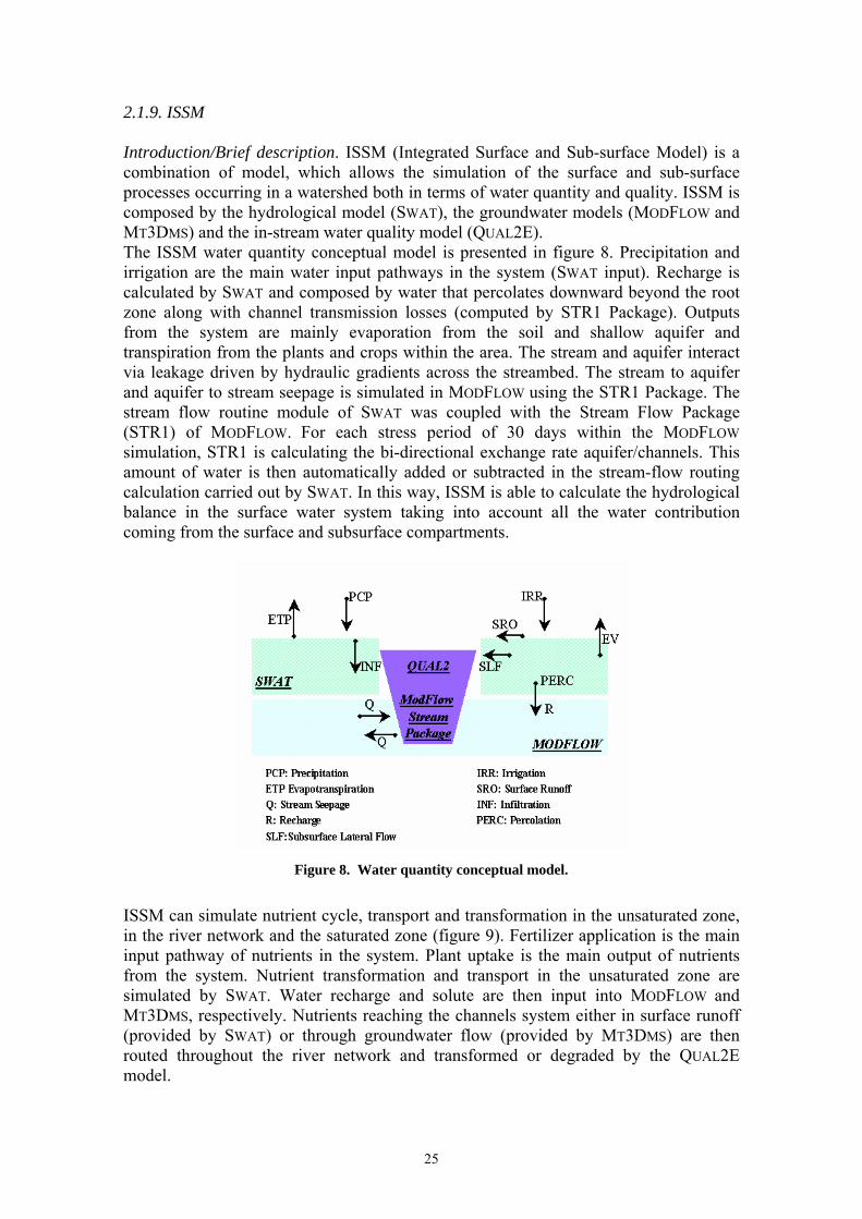
2.1.9. ISSM Introduction/Brief description. ISSM (Integrated Surface and Sub-surface Model) is a combination of model, which allows the simulation of the surface and sub-surface processes occurring in a watershed both in terms of water quantity and quality. ISSM is composed by the hydrological model (SWAT), the groundwater models (MODFLOW and MT3DMS) and the in-stream water quality model (QUAL2E). The ISSM water quantity conceptual model is presented in figure 8. Precipitation and irrigation are the main water input pathways in the system (SWAT input). Recharge is calculated by SWAT and composed by water that percolates downward beyond the root zone along with channel transmission losses (computed by STR1 Package). Outputs from the system are mainly evaporation from the soil and shallow aquifer and transpiration from the plants and crops within the area. The stream and aquifer interact via leakage driven by hydraulic gradients across the streambed. The stream to aquifer and aquifer to stream seepage is simulated in MODFLOW using the STR1 Package. The stream flow routine module of SWAT was coupled with the Stream Flow Package (STR1) of MODFLOW. For each stress period of 30 days within the MODFLOW simulation, STR1 is calculating the bi-directional exchange rate aquifer/channels. This amount of water is then automatically added or subtracted in the stream-flow routing calculation carried out by SWAT. In this way, ISSM is able to calculate the hydrological balance in the surface water system taking into account all the water contribution coming from the surface and subsurface compartments.

Figure 8. Water quantity conceptual model.

ISSM can simulate nutrient cycle, transport and transformation in the unsaturated zone, in the river network and the saturated zone (figure 9). Fertilizer application is the main input pathway of nutrients in the system. Plant uptake is the main output of nutrients from the system. Nutrient transformation and transport in the unsaturated zone are simulated by SWAT. Water recharge and solute are then input into MODFLOW and MT3DMS, respectively. Nutrients reaching the channels system either in surface runoff (provided by SWAT) or through groundwater flow (provided by MT3DMS) are then routed throughout the river network and transformed or degraded by the QUAL2E model.

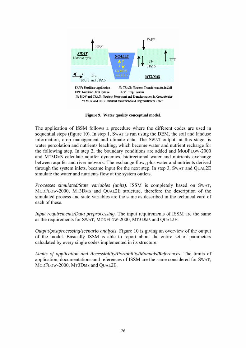
26

Figure 9. Water quality conceptual model.

The application of ISSM follows a procedure where the different codes are used in sequential steps (figure 10). In step 1, SWAT is run using the DEM, the soil and landuse information, crop management and climate data. The SWAT output, at this stage, is water percolation and nutrients leaching, which become water and nutrient recharge for the following step. In step 2, the boundary conditions are added and MODFLOW-2000 and MT3DMS calculate aquifer dynamics, bidirectional water and nutrients exchange between aquifer and river network. The exchange flow, plus water and nutrients derived through the system inlets, became input for the next step. In step 3, SWAT and QUAL2E simulate the water and nutrients flow at the system outlets. Processes simulated/State variables (units). ISSM is completely based on SWAT, MODFLOW-2000, MT3DMS and QUAL2E structure, therefore the description of the simulated process and state variables are the same as described in the technical card of each of these. Input requirements/Data preprocessing. The input requirements of ISSM are the same as the requirements for SWAT, MODFLOW-2000, MT3DMS and QUAL2E. Output/postprocessing/scenario analysis. Figure 10 is giving an overview of the output of the model. Basically ISSM is able to report about the entire set of parameters calculated by every single codes implemented in its structure. Limits of application and Accessibility/Portability/Manuals/References. The limits of application, documentations and references of ISSM are the same considered for SWAT, MODFLOW-2000, MT3DMS and QUAL2E.

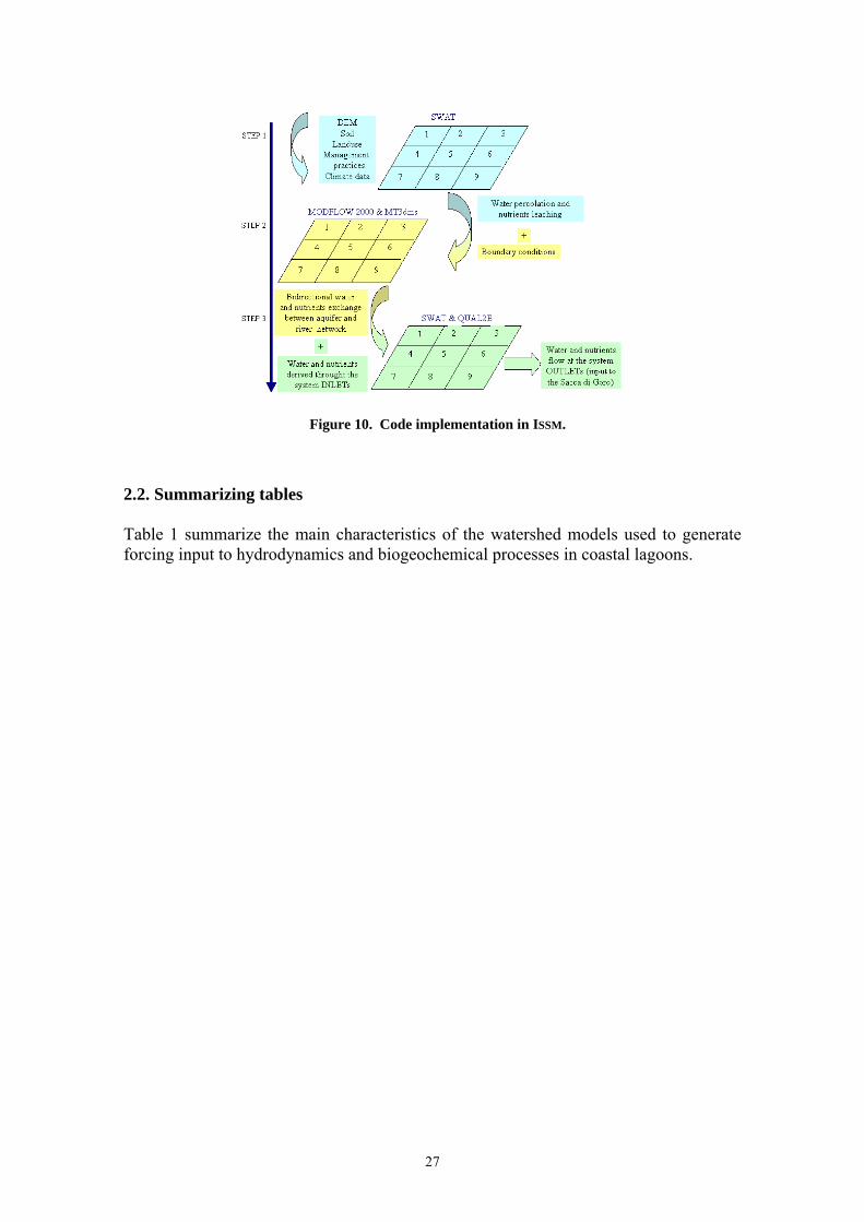
27

Figure 10. Code implementation in ISSM.

2.2. Summarizing tables Table 1 summarize the main characteristics of the watershed models used to generate forcing input to hydrodynamics and biogeochemical processes in coastal lagoons.

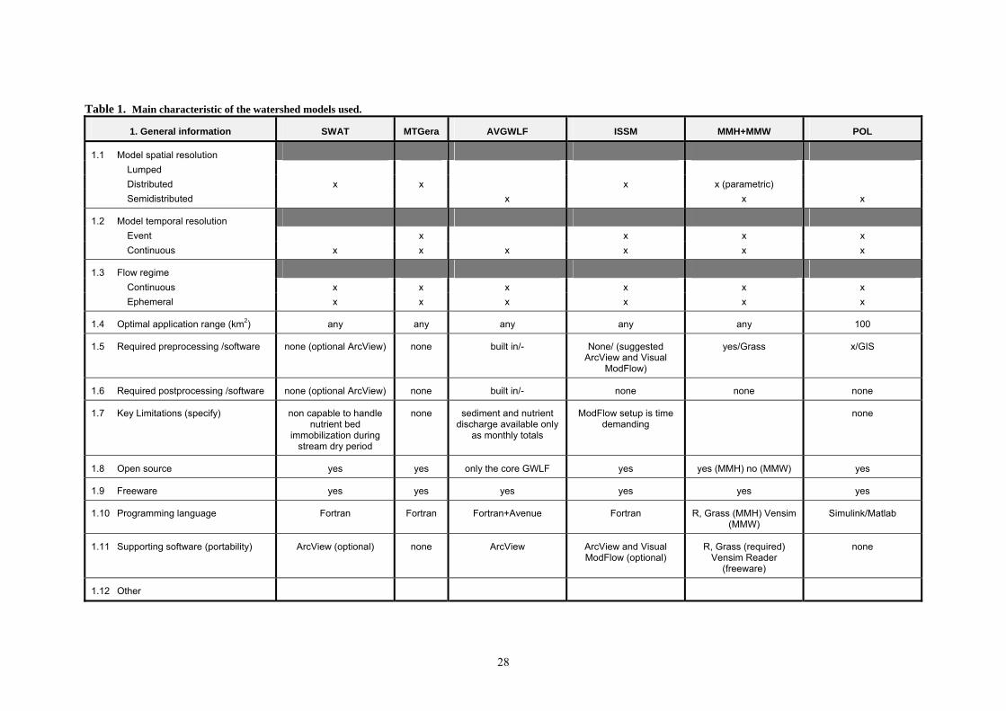
28

Table 1. Main characteristic of the watershed models used.

1. General information SWAT MTGera AVGWLF ISSM MMH+MMW POL

1.1 Model spatial resolution Lumped Distributed x x x x (parametric) Semidistributed x x x

1.2 Model temporal resolution Event x x x x Continuous x x x x x x

1.3 Flow regime Continuous x x x x x x Ephemeral x x x x x x

1.4 Optimal application range (km2) any any any any any 100

1.5 Required preprocessing /software none (optional ArcView) none built in/- None/ (suggested ArcView and Visual

ModFlow)

yes/Grass x/GIS

1.6 Required postprocessing /software none (optional ArcView) none built in/- none none none

1.7 Key Limitations (specify) non capable to handle nutrient bed

immobilization during stream dry period

none sediment and nutrient discharge available only

as monthly totals

ModFlow setup is time demanding

none

1.8 Open source yes yes only the core GWLF yes yes (MMH) no (MMW) yes

1.9 Freeware yes yes yes yes yes yes

1.10 Programming language Fortran Fortran Fortran+Avenue Fortran R, Grass (MMH) Vensim (MMW)

Simulink/Matlab

1.11 Supporting software (portability) ArcView (optional) none ArcView ArcView and Visual ModFlow (optional)

R, Grass (required) Vensim Reader

(freeware)

none

1.12 Other

29

Table 1 (contd). Main characteristic of the watershed models used.

2. Model Components SWAT MTGera AVGWLF ISSM MMH+MMW POL

2.1 Hydrological components

Rainfall / runoff x x x x x x Erosion /sediment x x x x x - Evapotranspiration x x x x x - Infiltration x x x x x - Deep percolation x - x x x - Soil water x - x x x - Groundwater x - x x - -

2.2 Pollution N/full cycle x/x x/- x/- x/x x/x x/- P/full cycle x/x x/- x/- x/x x/x x/- Pesticides/ full cycle

x/x -/- -/- x/x -/- -/-

Bacteria/ full cycle

x/x -/- -/- x/x -/- x/-

2.3 Diffuse source x x x x x x

2.4 Point source x x x x x x

2.5 Water quality analysis Runoff/subsurface x - x - - In-stream x - x x - Groundwater - - x - -

2.6 Crop growth Simple model - - - - - Detailed model x - x - -

2.7 Built-in scenario analysis

- - Predict (separate tool but interfaced)

x x (land use changes) -

2.9 Other

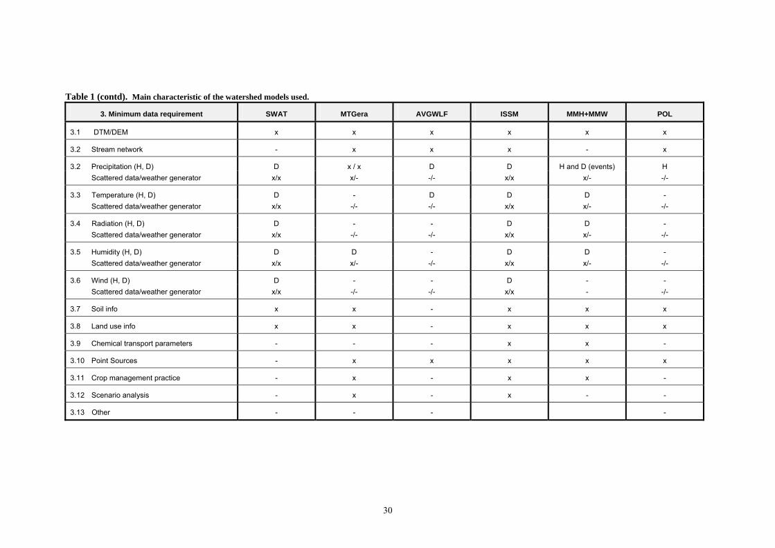
30

Table 1 (contd). Main characteristic of the watershed models used.

3. Minimum data requirement SWAT MTGera AVGWLF ISSM MMH+MMW POL

3.1 DTM/DEM x x x x x x

3.2 Stream network - x x x - x

3.2 Precipitation (H, D) D x / x D D H and D (events) H Scattered data/weather generator x/x x/- -/- x/x x/- -/-

3.3 Temperature (H, D) D - D D D - Scattered data/weather generator x/x -/- -/- x/x x/- -/-

3.4 Radiation (H, D) D - - D D - Scattered data/weather generator x/x -/- -/- x/x x/- -/-

3.5 Humidity (H, D) D D - D D - Scattered data/weather generator x/x x/- -/- x/x x/- -/-

3.6 Wind (H, D) D - - D - - Scattered data/weather generator x/x -/- -/- x/x - -/-

3.7 Soil info x x - x x x

3.8 Land use info x x - x x x

3.9 Chemical transport parameters - - - x x -

3.10 Point Sources - x x x x x

3.11 Crop management practice - x - x x -

3.12 Scenario analysis - x - x - -

3.13 Other - - - -

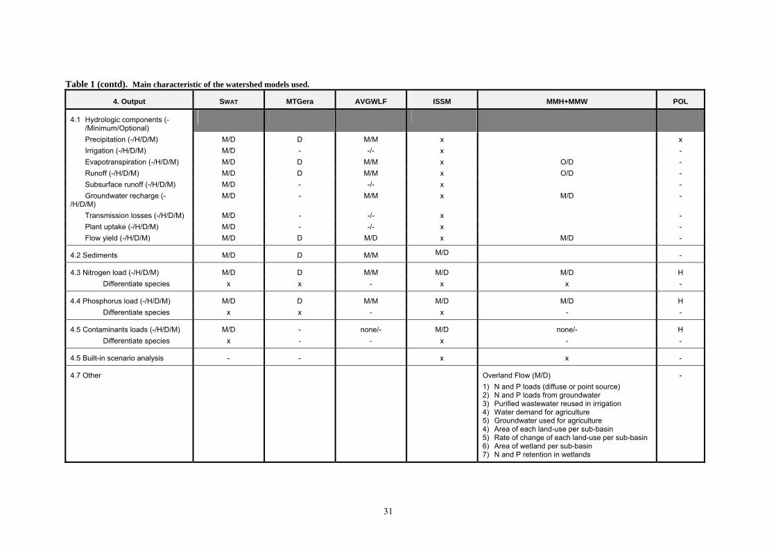
31

Table 1 (contd). Main characteristic of the watershed models used.

4. Output SWAT MTGera AVGWLF ISSM MMH+MMW POL

4.1 Hydrologic components (-/Minimum/Optional)

Precipitation (-/H/D/M) M/D D M/M x x Irrigation (-/H/D/M) M/D - -/- x - Evapotranspiration (-/H/D/M) M/D D M/M x O/D - Runoff (-/H/D/M) M/D D M/M x O/D - Subsurface runoff (-/H/D/M) M/D - -/- x - Groundwater recharge (-/H/D/M)

M/D - M/M x M/D -

Transmission losses (-/H/D/M) M/D - -/- x - Plant uptake (-/H/D/M) M/D - -/- x - Flow yield (-/H/D/M) M/D D M/D x M/D -

4.2 Sediments M/D D M/M M/D -

4.3 Nitrogen load (-/H/D/M) M/D D M/M M/D M/D H Differentiate species x x - x x -

4.4 Phosphorus load (-/H/D/M) M/D D M/M M/D M/D H Differentiate species x x - x - -

4.5 Contaminants loads (-/H/D/M) M/D - none/- M/D none/- H Differentiate species x - - x - -

4.5 Built-in scenario analysis - - x x -

4.7 Other Overland Flow (M/D) 1) N and P loads (diffuse or point source) 2) N and P loads from groundwater 3) Purified wastewater reused in irrigation 4) Water demand for agriculture 5) Groundwater used for agriculture 4) Area of each land-use per sub-basin 5) Rate of change of each land-use per sub-basin 6) Area of wetland per sub-basin 7) N and P retention in wetlands

-

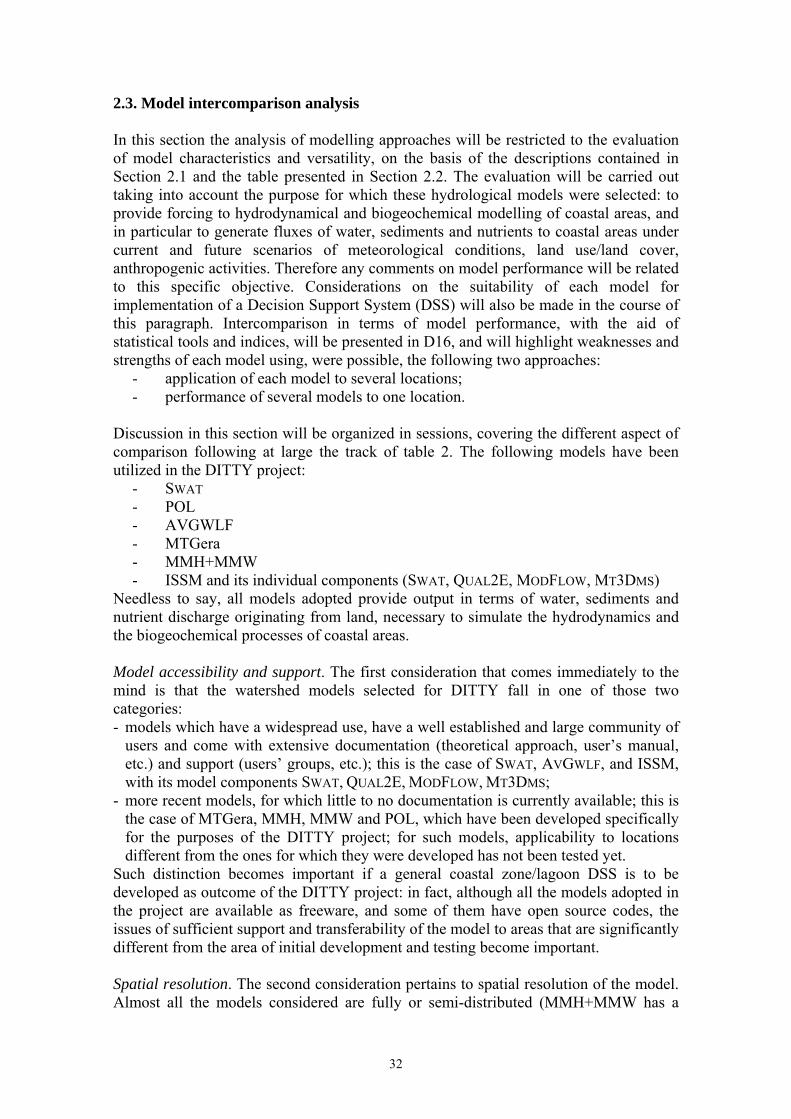
32

2.3. Model intercomparison analysis In this section the analysis of modelling approaches will be restricted to the evaluation of model characteristics and versatility, on the basis of the descriptions contained in Section 2.1 and the table presented in Section 2.2. The evaluation will be carried out taking into account the purpose for which these hydrological models were selected: to provide forcing to hydrodynamical and biogeochemical modelling of coastal areas, and in particular to generate fluxes of water, sediments and nutrients to coastal areas under current and future scenarios of meteorological conditions, land use/land cover, anthropogenic activities. Therefore any comments on model performance will be related to this specific objective. Considerations on the suitability of each model for implementation of a Decision Support System (DSS) will also be made in the course of this paragraph. Intercomparison in terms of model performance, with the aid of statistical tools and indices, will be presented in D16, and will highlight weaknesses and strengths of each model using, were possible, the following two approaches:

- application of each model to several locations; - performance of several models to one location.

Discussion in this section will be organized in sessions, covering the different aspect of comparison following at large the track of table 2. The following models have been utilized in the DITTY project:

- SWAT - POL - AVGWLF - MTGera - MMH+MMW - ISSM and its individual components (SWAT, QUAL2E, MODFLOW, MT3DMS)

Needless to say, all models adopted provide output in terms of water, sediments and nutrient discharge originating from land, necessary to simulate the hydrodynamics and the biogeochemical processes of coastal areas. Model accessibility and support. The first consideration that comes immediately to the mind is that the watershed models selected for DITTY fall in one of those two categories: - models which have a widespread use, have a well established and large community of

users and come with extensive documentation (theoretical approach, user’s manual, etc.) and support (users’ groups, etc.); this is the case of SWAT, AVGWLF, and ISSM, with its model components SWAT, QUAL2E, MODFLOW, MT3DMS;

- more recent models, for which little to no documentation is currently available; this is the case of MTGera, MMH, MMW and POL, which have been developed specifically for the purposes of the DITTY project; for such models, applicability to locations different from the ones for which they were developed has not been tested yet.

Such distinction becomes important if a general coastal zone/lagoon DSS is to be developed as outcome of the DITTY project: in fact, although all the models adopted in the project are available as freeware, and some of them have open source codes, the issues of sufficient support and transferability of the model to areas that are significantly different from the area of initial development and testing become important. Spatial resolution. The second consideration pertains to spatial resolution of the model. Almost all the models considered are fully or semi-distributed (MMH+MMW has a

33

semi-distributed/parametric approach). Therefore, spatial variability of morphological characteristics, land use/land cover, soil, characteristics, etc. are taken into account, either in detail by subdividing the study area in sub-catchments and hydrological response units, or by somehow computing a separate response for each main combination of watershed characteristics, or simply by discretising the modelling domain into cells. Such feature is extremely essential to an effective performance of scenario analysis including source apportionment, as possibly embedded in the DSS under development. Theoretical approach. As it is apparent from the descriptions presented in the previous sections, the theoretical approaches adopted in all the models to describe the hydrological and transport processes that participate in the formation of water, sediment and nutrient discharge to coastal areas, are sometimes quite similar and other times quite different. POL approach is quite different. As it does not run separately flows and concentration it does not simulate runoff. It simulates dissolved nitrogen and phosphorus load. Excepting POL, all models apply the SCS CN method for calculation of runoff and the some form of the USLE method for calculation of the rainfall erosion. All models simulate all components of the hydrological cycle except for MTGera which uses the CN-MUSLE approach for rainfall/runoff transformation and couples it with some specifically tailored functions for calculation of sediment and nutrient concentrations, and MMH, which uses the approach of the Unit Hydrograph (parametric approach) to generate discharges. Calculation of evapotranspiration is performed using the any of the following equation: Turc (MMH), Blaney and Criddle or Hammon (AVGWLF), Penman-Monteith, Priestley-Taylor or Hargreaves (SWAT). All models calculate N and P discharge, but only SWAT, ISSM and MMH-MMW include simulation of the full N and P cycles. Only SWAT (and ISSM) include a detailed crop-growth model and allows to select land and crop management operations. AVGWLF is equipped with the Predict tool, a user-friendly scenario-analysis tool which allows preliminary assessment of pre-set and custom-made best management practices using some simple parametric expression for cost/benefit analysis. Only MMH-MMW has built-in functions for scenario analysis, while in the case of the other models scenario analysis can be performed by running the full model repeatedly under different set of input parameters. All the theoretical approaches adopted have a long standing acceptance within the scientific community and the choice of one approach over another one depends on the characteristics of the study area and on the availability of data. As already stated, applicability of MTGera and MMH+MMW at large has not been tested. Therefore their suitability for use within a general DSS needs to be verified. Pre- and postprocessing and input and output requirements. The availability of a user-friendly interface for model input, run and, where possible, postprocessing, is an issue that needs careful consideration where inclusion of the model in a DSS is concerned. Fully distributed models, such as SWAT and ISMM, require a very detailed description of the modelling domain, including extensive meteorological series, soil composition and hydrological properties, space and time description of point and diffuse source, land and crop management practices, just to name the essential ones; furthermore, for some of these models, the data input interfaces are not always user-friendly and involve the use of specific GIS software for handling of databases and spatially distributed data. The requirement of broad expertise and large availability of data can make such models largely unsuitable for application within the frame of a DSS. Compared to SWAT and ISSM, AVGWLF and POL have a relatively simpler input requirement and data handling

34

interface, and it could be more suitable for the frame of a DSS. All models produce daily outputs of water, sediment and nutrient discharges to the coast, in some instances with some form of source or area apportionment. Only in the case of AVGWLF, nutrient and sediment loads are delivered as monthly loads. In light of the issues discussed above, selection of the most appropriate model is difficult. All models have a strong an dwell established scientific basis. The main concerns in the choice are data requirement and handling, easiness of use, output characteristics. Another issue, not covered here, is the easiness of coupling with the hydrodynamic and biogeochemical modules within the frame of a DSS. Selection of the most appropriate model should follow comparative assessment of model performance, as presented in Deliverable 16.

35

3. HYDRODYNAMIC MODELLING Hydrodynamic models are tools built to describe and/or forecast fluid flow and related variables (T, S, TKE, etc.) for a given environment (ocean, continental shelf, lagoon, etc.). The well known Navier-Stokes’ equations are the base for mathematical modelling of geophysical fluid dynamics. Unfortunately such kind of non-linear partial differential equations are very difficult to solve. Instead, a simplified form of the equations, known as Boussinesq equations, are often used in the field of oceanography to build mathematical models. That system of equation (Nihoul, 1975) derived from classical mechanics theory needs a turbulent closure (Mellor and Yamada, 1982) and a state equation for sea water (Gill, 1982) in order to be solved. Present mathematics fails to provide solutions to that system of equations but numerical techniques can be applied with success in this case. Of course initial and boundaries conditions need to be specified. Example of such a model can be found in Luyten et al. (1999) while application to the North Sea is presented in Luyten et al. (2003). Hydrodynamic processes are present at all time and space scale in the ocean and models setups need to take such scale parameter into consideration. For the purposes of the DITTY project, the hydrodynamic modelling has to work in the so-called meso-scale domain. The support of the model or its dimension in the physical space is also a feature of the model. Saying all this, one can understand why all hydrodynamic models presented here are based on the same systems of equations. This is probably one of the main differences between hydrodynamic and biogeochemical models. The former are all based on same equations, while the latter use different equations derived from different parameterisation of concepts and/or observed processes. The modelling philosophy of DITTY was from one hand to use existing models for given site and from the other hand to develop common modelling tools. Following that philosophy, we present here three different hydrodynamical three-dimensional models. Even though they are all based on same equations, they use different turbulent closures, different kinds of boundary condition, or numerics: - MARS from IFREMER is applied to the Thau lagoon (FR). - COHERENS from MUMM is applied to Sacca di Goro site (IT) - POM-Gera from AEGEAN University is applied on Gera Bay (GR). One two-dimensional model is also presented by UFP for its application to Ria Formosa. Hydrodynamic models solve generally advection and diffusion phenomena on momentum, buoyancy and turbulent kinetic energy. Some models include also the possibility to add local production or destructions terms for biogeochemical processes in a passive tracer equation. That is the way followed when coupling biogeochemistry to hydrodynamics (see the example of Sacca di Goro). A brief presentation of the different models is given in the following paragraphs, illustrating in particular required input data and parameter to start a run of the given model. The description is followed by a table where each of the four models is compared to the others in terms of their different features and requirements.

36

Deliverable D16 will include inter-comparison study between MARS and COHERENS on Thau lagoon and the inter-comparison between POM and COHERENS on gulf of Gera. 3.1. Presentation of the tools employed 3.1.1. COHERENS COHERENS is a three-dimensional multi-purposes model dedicated to coastal and shelf seas (Luyten et al.,1999). The spectral window of this model is open to meso-scale and synoptic phenomena. Boussinesq equations are solved using hydrostatic assumption on a vertically transformed sigma space. Free surface elevation is considered. Horizontal diffusion is treated as Fick’s law while on the vertical a complete turbulent closure scheme is proposed including several different parameterizations. Horizontal sub-grid scales phenomenon are treated as turbulent process. Numerical includes mode splitting technique to separate external 2D from internal 3D modes. The model can be forced at the air-sea boundary by different parameterizations of wind stress and heat flux a number of data are needed for each case. At all open boundaries (open sea, rivers) several conditions can be applied as well. Some data are also required depending of the choice of the user. The model has been used on numerous different sites with good success and is available free of charge for scientific purposes. As a general matter, COHERENS solves an advection-diffusion equation such as:

(5) where Y is a given scalar that can be temperature, salinity, or biogeochemical state variable, u being the velocity vector, SY the specific movement of Y and ν the parameter for the diffusion. P(Y) and D(Y) are any biogeochemical productions or destructions terms respectively. In his actual form COHERENS include also a biological model characterizing primary production for a North Sea application. A particle tracking and a contaminant module exist as well as a sediment transport routine. The available code (version 8.4) is written in FORTRAN. The code is in the form of a collection of subroutines called by a main program. A makefile used for compilation is also provided. Information and orders (COHERENS is free of charge for scientific use) can be requested through the web site http://www.mumm.ac.be/COHERENS/. A complete documentation of almost 1000 pages is available on the COHERENS CDROM (pdf format). That documentation describes all aspect of the physics and the code, including requirements for boundary conditions, as well as few examples of uses; it also includes input and outputs files to run these examples. Even if the code is highly portable, a specific version for UNIX and WINDOWS is available from the COHERENS CDROM. 3.1.2. POM POM is a general circulation model that solves the equations of motion and mass and heat conservation (the so-called primitive equations) with finite differences on an

Y .( Y) .( Y) [ P(Y) - D(Y) ] . ( Y)t

υ∂+ ∇ + ∇ = + ∇ ∇

∂ Yu S

37

Aracawa C grid (Blumberg and Mellor, 1987). The code is written in FORTRAN 77. It is suitable for coastal seas, as it employs the sigma-coordinate (terrain-following) system for the discretisation of the vertical dimension. Besides the free sea surface elevation that is treated as a prognostic variable, the model calculates the temperature, salinity, the average and the 3D velocity fields and the turbulent kinetic energy.

Forcing requirements. The major circulation-forcing physical mechanisms (exchange of momentum, heat and water with the atmosphere, freshwater from rivers, tides) need to be taken into account for a meaningful simulation study: the model is driven by realistic daily wind stresses, calculated from meteorological observations of wind speed and direction (momentum fluxes); the tide (semi-diurnal for the study area with max amplitude of 0.6m) is applied at the south open boundaries. The tidal signal is simulated as the sum of four simple harmonic (sine or cosine wave) constituents, each of which has its own characteristic period, phase and amplitude and corresponds to the four most important constituent forces (Arhonditsis et al., 2000; 2002). Boundary conditions. The modelling domain is defined by the bathymetry, the open boundary in the south connecting the gulf to the Aegean and the sea surface. The temperature and salinity distributions on a daily basis are required to run the application (a) on the sea surface and (b) on a vertical plane separating the gulf with the open sea. These distributions are calculated by spatial and temporal interpolation using field data collected from a network of seven stations on a monthly basis. Numerical aspects. POM solves the so-called primitive equations with finite differences on an Aracawa C grid. It uses a time splitting technique in order to save computation time: different time step for the solution of the 2D (barotropic) and the 3D (baroclinic) equations. The horizontal turbulent (eddy) viscosity and diffusivity is parameterized through the Smagorinsky formulation, thus the horizontal mixing depends on the grid size and the horizontal velocity fields. The vertical turbulent viscosity/diffusivity parameter is calculated by the Mellor and Yamada turbulence closure scheme. Input/Output. Input and output is in the form of matrices (text files). The presentation of the results in the current application is being carried out using MATLAB. Limits of application. The limits of application depend on the availability of data. Accessibility/Portability/Manuals/References. The POM code is accessible through the POM website. It can be run on any machine (PC, Unix, Linux) running Standard FORTRAN 77. Model details such as equations involved, solution techniques, relative references can be found in Mellor (1996) and at www.aos.princeton.edu/WWWPUBLIC/htdocs.pom. For the current application, details have been given by Kolovoyiannis et al. (2005). 3.1.3. MARS3D The MARS3D hydrodynamic model was developed at Ifremer about ten years ago (Lazure and Jégou, 1998). Initially for studying the Atlantic seaboard, the model has been applied to other regions, notably the Mediterranean sea. Its application to the Thau lagoon was done as part of the ‘Mediterranean lagoons’ case study by the PNEC (Lazure, 1992). This three dimensional model is designed to represent, as faithfully as

38

possible, the transportation and mixing of bodies of water on time scale varying from an hour to a day (at least). Forcing requirements. The lagoon dynamics cover two closely linked aspects. These are the water movements within the lagoon and the exchanges with the sea via the Sete channels. The wind is the principal generator of currents within the lagoon. Density currents (due to fresh water inputs by the rivers in rainy periods) are considered as much weaker or highly localised because of the small volumes of water involved. The dynamics of exchanges with the sea are controlled by three fundamental factors whose influences are mutually superimposed. These are the tide, the atmospheric pressure and the wind. The exchanges have a special importance because they maintain the marine character of the Thau lagoon. Fresh water inputs are generally small, but can occasionally be very great because of the climate. This occurs when the many rivers in the Thau catchment area flood. The bathymetric data used to define the calculation grid were collected between 1984 and 1987 (SHOM Data). The wind and pressure data are from Meteo France recorded at the Station météorologique de Sète and where possible measured on the lagoon from 2002 (Data Université de Montpellier II). Boundary conditions. Requirements at the open boundaries of the domain are the knowledge of sea surface position, salinity and temperature, at any time step. As this model is more and more used coupled with biogeochemical models over coastal areas, it must be able to account for river discharge. Numerical aspects. As COHERENS and POM, MARS belongs to the “3D model in sigma coordinates” class of hydrodynamic models. The model uses a numerical scheme with finite differences to resolve the primitive equations of fluid mechanics under hydrostatic and Boussinesq approximations. The model uses a barotropic-baroclinic mode splitting approach. The equations are solved using the technique of internal and external surface modes separation. The external mode solves equations integrated on the vertical, which reproduce gravity waves. The internal mode collects information from the external mode (surface free, integrated currents) and resolves equations on the vertical (three-dimensional current structure). Accessibility/Portability/Manuals/References. The model runs on Unix/Linux platforms. Publication describing the hydrodynamic model and its application on a French Bay are in preparation. 3.1.4 RF2D Hydrodynamics - EcoDynamo The model was implemented with EcoDynamo (Pereira and Duarte, 2005) - an object-oriented modelling software written in C++. There are different objects to simulate hydrodynamic, thermodynamic and biogeochemical processes and variables. The shell interface allows the user to choose among different models and to define the respective setups – time steps, output formats (file, graphic and tables), objects to be used and variables to be visualised. The list of objects, variables and parameters of model equations are stored in specific files. Objects may communicate among them for data exchange.

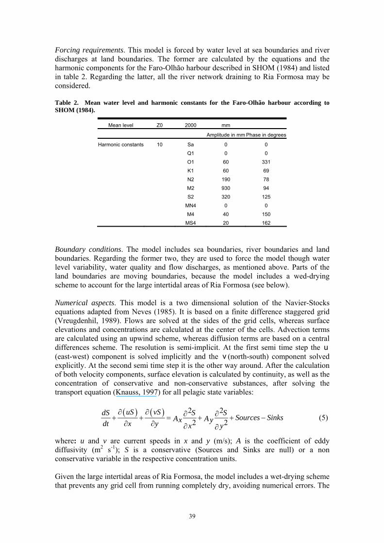
39

Forcing requirements. This model is forced by water level at sea boundaries and river discharges at land boundaries. The former are calculated by the equations and the harmonic components for the Faro-Olhão harbour described in SHOM (1984) and listed in table 2. Regarding the latter, all the river network draining to Ria Formosa may be considered. Table 2. Mean water level and harmonic constants for the Faro-Olhão harbour according to SHOM (1984).

Mean level Z0 2000 mm

Amplitude in mm Phase in degrees

Harmonic constants 10 Sa 0 0

Q1 0 0

O1 60 331

K1 60 69

N2 190 78

M2 930 94

S2 320 125

MN4 0 0

M4 40 150

MS4 20 162

Boundary conditions. The model includes sea boundaries, river boundaries and land boundaries. Regarding the former two, they are used to force the model though water level variability, water quality and flow discharges, as mentioned above. Parts of the land boundaries are moving boundaries, because the model includes a wed-drying scheme to account for the large intertidal areas of Ria Formosa (see below). Numerical aspects. This model is a two dimensional solution of the Navier-Stocks equations adapted from Neves (1985). It is based on a finite difference staggered grid (Vreugdenhil, 1989). Flows are solved at the sides of the grid cells, whereas surface elevations and concentrations are calculated at the center of the cells. Advection terms are calculated using an upwind scheme, whereas diffusion terms are based on a central differences scheme. The resolution is semi-implicit. At the first semi time step the u (east-west) component is solved implicitly and the v (north-south) component solved explicitly. At the second semi time step it is the other way around. After the calculation of both velocity components, surface elevation is calculated by continuity, as well as the concentration of conservative and non-conservative substances, after solving the transport equation (Knauss, 1997) for all pelagic state variables:

( ) ( ) 2 22 2

uS vSdS S S Sources SinksA Ax ydt x y x y

∂ ∂ ∂ ∂+ + = + + −∂ ∂ ∂ ∂

(5)

where: u and v are current speeds in x and y (m/s); A is the coefficient of eddy diffusivity (m2 s-1); S is a conservative (Sources and Sinks are null) or a non conservative variable in the respective concentration units. Given the large intertidal areas of Ria Formosa, the model includes a wet-drying scheme that prevents any grid cell from running completely dry, avoiding numerical errors. The

40

general approach is to stop using the advection term when depth is lower than a threshold value (0.1 m in the present case) to avoid numerical instabilities. Below this threshold and until a minimum limit of 0.05 m, the model computes all remaining terms. When this limit is reached, computations do not take place in a given cell until a neighbour cell has a higher water level, allowing then the pressure term to start “filling” the “dry” cell. The wet-drying scheme requires a relatively high spatial and temporal resolution. In the present case, the former is 100 m and the latter 3 s. A lower temporal resolution leads to numerical errors, in spite of the semi-implicit numerical scheme of the hydrodynamic model. Problems arise when there is a relatively large depth difference between two extremes of an intertidal grid cell. In this case, cell volume may be relatively small and advection through the deeper side may produce a negative volume, unless the proper time step is chosen. Therefore, the model requires a large computing time. Input/Output. The mandatory input files needed to initialise and run the model are:

1. Morphology File - describes the morphology of the ecosystem, including the number of cells, localisation, geometry and boundary types.

2. Classes File - lists all classes/objects that can be used by the simulation. 3. Variables File - lists the variables treated by each class/object and their initial

values. 4. Parameters File - lists the parameters used by each class and their initial,

minimum, maximum and increment values. The next files are not mandatory but can be useful in some ecosystems or simulations:

5. Loads File - requested when loads are considered. 6. Points File – to define subdomains. 7. Rivers Files – to define river locations and daily river flows 8. Sediments File – to define sediment types and locations within the model grid

All these files are saved in text format, with tab-separated values, and can be accessed and modified by any text editor or commercial application (Excel, Word, Wordpad, Notepad, etc.). The name of the first five files must have a common prefix; the suffix distinguishes the file type. The results can be saved in a General Output File or Mean Values Files. The General Output File has, by default, 3 formats: "xls", "hdf" or "txt". The "xls" and "txt" formats are text files saved with tabs separating values. The "xls" format is used for Excel application quick view with Tab Separated Values. The first five columns are fixed for all registers: time (in hours), model time step, column (east-west grid coordinate), line (north-south grid coordinate) and cell numbers. The next columns contain the results for the selected variables. The "hdf" format follows the HDF specifications - see NCSA http server (http://hdf.ncsa.uiuc.edu/). Generating Mean Values Files enables the user to run the model with a minor time step (normally only the hydrodynamic part of the model) and save the mean flow and velocity values in files, integrated over a time period under the choice of the user. The Mean Values Files are formatted as "xls" files and their names follow a special order. The first three columns are fixed for all registers: time (in seconds from January 1, 1970 00:00), register step and cell number. The next columns are filled with time-averaged results.

41

Apart from file output, graphical output using a MatLab server application is also available. More details on input/output may be found in Pereira and Duarte (2005). Limits of application. The hydrodynamic model is generally applicable to shallow-water coastal ecosystems. Accessibility/Portability/Manuals/References. Accessibility: The model is generally available for research purposes. The model runs on Windows platforms. Reports describing the hydrodynamic model and the software EcoDynamo are available from the authors upon request - Duarte et al. (2005a); Pereira and Duarte (2005) – and from http://www.dittyproject.org/reports.asp. 3.2. Summarizing tables The following table summarizes the main characteristics of the four hydrodynamic models using for simulating the hydrodynamics in coastal lagoons.

42

Table 3. Main characteristic of the hydrodynamic models used.

Characteristics COHERENS (Sacca di Goro, IT) MARS (Thau lagoon, FR) POM (Gulf of Gera, GR) Ecodyn (Ria Formosa, PT)

Dimensions 0D/1D/2D/3D 3D 3D 2D

Grid type Orthogonal/curvilinear Orthogonal Orthogonal (56 x 151 gridpoints, 100m cell) Orthogonal

Vertical geometry Sigma Sigma Sigma , σ = (z - η) / (Η + η), H:bathymetry, η: sea surface elevation

Z

Time scale Meso-scale hourly, daily, monthly Two modes: Barotropic mode 1s, Baroclinic mode 30 s. Time simulated: annual cycle (14 months)

Time step 3 s, Simulated periods - from seconds to months

Boussinesq approximation Yes Yes Yes -

Mode splitting Yes Yes Yes No

Hydrostatic assumption Yes Yes Yes -

State variables Velocity (3 components), T, S, Surface elevation, Turbulent model components

T, S, V, free surface elevation

Temperature (potential), Salinity, Velocity (3 components U,V,W), Sea-surface elevation, Turbulent Kinetic Energy, Turbulent macroscale (mixing length)

Horizontal velocity components, Water level, Salinity and derived variables such as flow.

Input format ASCII for bathymetry and forcing (meteorological, open sea, watershed)

ASCII (Meteorological forcing data); Netcdf (bathymetry)

Txt or .dat files in the form of matrices Text

Output format COHERENS format or Netcdf Netcdf Txt or .dat files in the form of matrices Text, Hierarchical Data Format (*.hdf files), Graphical output using MATLAB graphical functions.

Graph software used IDL, MATLAB, Ferret MATLAB MATLAB MATLAB

Turbulence closure schemes

Algebraic formula, one or two equations Mellor & Yamada (1982), k-ε Rodi (1984), Luyten et al (1996)

k-kl turbulence closure Model. (Mellor and Yamada 1982)

k, l Mellor-Yamada submodel Mellor and Yamada (1982)

Constant dispersion coefficient

State equation for seawater Linearised equation or UNESCO general formula for sea water state (Fofonoff, 1985)

rho = F(S,T,p) with either F linearised around a point (T0,S0,p=0) or F fully developed in the Mellor (1991).

The UNESCO equation of state, as adapted by Mellor (1991).

Cox et al (1970) for Salinity > 10 and Knudsen (1901) for Salinity <= 10.

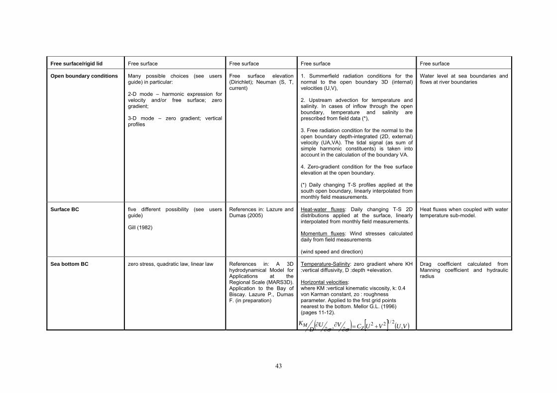
43

Free surface/rigid lid Free surface Free surface Free surface Free surface

Open boundary conditions Many possible choices (see users guide) in particular:

2-D mode – harmonic expression for velocity and/or free surface; zero gradient;

3-D mode – zero gradient; vertical profiles

Free surface elevation (Dirichlet); Neuman (S, T, current)

1. Summerfield radiation conditions for the normal to the open boundary 3D (internal) velocities (U,V),

2. Upstream advection for temperature and salinity. In cases of inflow through the open boundary, temperature and salinity are prescribed from field data (*),

3. Free radiation condition for the normal to the open boundary depth-integrated (2D, external) velocity (UA,VA). The tidal signal (as sum of simple harmonic constituents) is taken into account in the calculation of the boundary VA.

4. Zero-gradient condition for the free surface elevation at the open boundary.

(*) Daily changing T-S profiles applied at the south open boundary, linearly interpolated from monthly field measurements.

Water level at sea boundaries and flows at river boundaries

Surface BC five different possibility (see users guide)

Gill (1982)

References in: Lazure and Dumas (2005)

Heat-water fluxes: Daily changing T-S 2D distributions applied at the surface, linearly interpolated from monthly field measurements.

Momentum fluxes: Wind stresses calculated daily from field measurements

(wind speed and direction)

Heat fluxes when coupled with water temperature sub-model.

Sea bottom BC zero stress, quadratic law, linear law References in: A 3D hydrodynamical Model for Applications at the Regional Scale (MARS3D). Application to the Bay of Biscay. Lazure P., Dumas F. (in preparation)

Temperature-Salinity: zero gradient where KH :vertical diffusivity, D :depth +elevation.

Horizontal velocities: where KM :vertical kinematic viscosity, k: 0.4 von Karman constant, zo : roughness parameter. Applied to the first grid points nearest to the bottom. Mellor G.L. (1996) (pages 11-12).

Drag coefficient calculated from Manning coefficient and hydraulic radius

( ) [ ] ( )VUVUCVUD

KZM ,,

2/122 +=∂∂

∂∂

σσ

44

Vertical velocity ω : ω (-1) = 0

Other modules available all available see users guide for details Particle tracking/biology (primary production, bacteria contamination, oysters), Oxygen (anoxic crisis)/passive tracers

1. A 7-state variable, pelagic, ecological submodel coupled

2. A watershed submodel, evaluating point and non-point nutrient and organic matter loading from terrestrial sources.

Biological and sediment transport sub-models

Data requirements bathymetry, atmospheric forcing, initial and boundaries conditions

Input files of : bathymetry, initial T-S 3D distributions, surface, distributions of T-S used as surface BC, vertical profiles of T-S used as open BC, wind speed-direction (analyzed to x- and y- components)

Bathymetry, Tidal harmonics, River flows

References to the users guide of the model

Luyten et al., 1999. Lazure and Dumas, 2005. Lazure and Salomon, 1991.

Mellor, 1996. http://www.aos.princeton.edu/WWWPUBLIC/htdocs.pom/userinfo.htm

Pereira and Duarte, 2005.

Other http://www.mumm.ac.be/coherens/ Lazure (1992) http://www.aos.princeton.edu/WWWPUBLIC/htdocs.pom

Duarte et al., 2005.

{ }[ ] ⎥⎥⎦

⎤

⎢⎢⎣

⎡

+=

−0025.0,

/)1(ln 21

2

okbZ

zHkMAXC

σ

45

3.3. Model intercomparison analysis In this part of the work the model intercomparison analysis will be restricted to the evaluation of basic hydrodynamic model characteristics given in the summarizing table (Section 3.2) and also on the information provided into summaries and abstracts for performances of the employed modelling tools (Section 3.1). A detailed intercomparison analysis based on statistical estimation of differences between numerical results obtained with different models as in Beckers et al. (2002) will be the object to D16 report and it will be limited to the sites were two hydrodynamic models have been developed and implemented using the same initial and forcing conditions, i.e. Thau lagoon and gulf of Gera. In DITTY project four hydrodynamic/physical models have been applied as follow:

• COHERENS for Sacca di Goro lagoon • MARS3D for Etang de Thau lagoon • POM for Gera gulf • EcoDynamo for Ria Formosa lagoon.

For the fifth project test site (Mar Menor) actually hydrodynamic model has been not developed and only a 0D ecological model has been used. For that reason the above mentioned hydrodynamic models will be taken into consideration in the analysis below. The first conclusion which arises after comparison of model characteristics is that EcoDynamo model, as only 2D vertically integrated model, completely differs from the other 3D models. However, the EcoDynamo is the best choice for Ria Formosa case because this lagoon in fact presents a complicated system of connected channels with altered width. Further, in between the applied models, only the EcoDynamo model comprises at present an option to switch wet/dry computation cells which is an important and absolutely needed procedure for modelling of water bodies as Ria Formosa lagoon affected by severe flooding and ebb tides. Then, our further conclusions concerning intercomparison analysis will be more focus on the 3D models but also will consider the EcoDynamo model in some specific model aspects as model boundary conditions, input, output and visualisation of model results. Further, all the 3D hydrodynamic models used in DITTY (COHERENS, MARS3D and POM) are developed under nowadays commonly accepted and quite similar oceanographical assumptions. As consequence these models differ slightly, have analogous characteristics and could be thought as almost compatible. For example the three models are build under Boussinesq approximation and vertical hydrostatic equilibrium assumption, include 3 velocity components, temperature, salinity, UNESCO equation for seawater state, identical turbulence closure scheme (equation for turbulent kinetic energy) and count for free surface changes. Additionally, the models use sigma transformed vertical space, orthogonal horizontal grid, mode splitting technique and resolve seasonal and meso-scale time processes. In respect of model data requirements (bathymetry, atmospheric forcing, watershed impact, etc.), sea surface and bottom boundary conditions, initial conditions and coupling with additional modules (ecological, biological, sediment etc.) one can conclude that all models (including EcoDynamo) demonstrate quite similar potential and they altogether have flexible and open structure which allow user define modifications, additions, changes etc. to be easily incorporated into the model code platform/configuration. None of the models has build inside user friendly input/output

46

procedure or software (something really very difficult for oceanographic models) but all models have wide spectra of input/output options based on ASCII or BINARY files and in this sense provide good opportunity for later on using graphical software as MATLAB, IDL or FERRET. Furthermore, the entire set of hydrodynamic models used in DITTY is relatively well documented, for some of them Internet sites and discussion forum are available (COHERENS and POM). All original model versions are tested, calibrated and verified by each model development team and last but not least some of the models (COHERENS and POM) have the advantage to be freely distributed for scientific purposes. Finally, in the group of considered models COHERENS demonstrates some theoretical and structural advantages as: possibility of using curvilinear coordinate system, availability of few turbulence schemes (algebraic or with one and two equations), a larger variety of open boundary conditions, more options for surface and bottom boundary conditions and few numerical engines. Nevertheless, the performances of all intercompared models are good and it is not possible to state that one of the models could be favoured or prioritized. However, we believe that COHERENS with an option to switch wet/dry computation cells and with an object oriented approach to include ecological modules could become a standard for coastal lagoons. In summary, the intercomparison analysis about simulations of coastal water bodies studied in DITTY show that all of the applied hydrodynamic models have sound and common theoretical background, flexible and well organize structure, well reproduce spatial and temporal dynamics of coastal zone systems and none of the models could be favoured or prioritized because the models altogether produce almost compatible results.

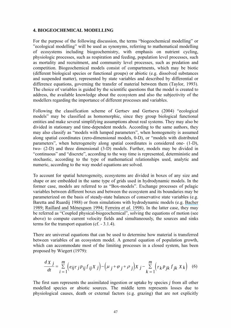
47

4. BIOGEOCHEMICAL MODELLING For the purpose of the following discussion, the terms “biogeochemical modelling” or ”ecological modelling” will be used as synonyms, referring to mathematical modelling of ecosystems including biogeochemistry, with emphasis on nutrient cycling, physiologic processes, such as respiration and feeding, population level processes, such as mortality and recruitment, and community level processes, such as predation and competition. Biogeochemical models consist of compartments, which may be biotic (different biological species or functional groups) or abiotic (e.g. dissolved substances and suspended matter), represented by state variables and described by differential or difference equations, governing the transfer of material between them (Taylor, 1993). The choice of variables is guided by the scientific questions that the model is created to address, the available knowledge about the ecosystem and also the subjectivity of the modellers regarding the importance of different processes and variables. Following the classification scheme of Gertsev and Gertseva (2004) “ecological models” may be classified as homomorphic, since they group biological functional entities and make several simplifying assumptions about real systems. They may also be divided in stationary and time-dependent models. According to the same authors, they may also classify as “models with lumped parameters”, when homogeneity is assumed along spatial coordinates (zero-dimensional models, 0-D), or “models with distributed parameters”, when heterogeneity along spatial coordinates is considered one- (1-D), two- (2-D) and three dimensional (3-D) models. Further, models may be divided in “continuous” and “discrete”, according to the way time is represented, deterministic and stochastic, according to the type of mathematical relationships used, analytic and numeric, according to the way model equations are solved. To account for spatial heterogeneity, ecosystems are divided in boxes of any size and shape or are embedded in the same type of grids used in hydrodynamic models. In the former case, models are referred to as “Box-models”. Exchange processes of pelagic variables between different boxes and between the ecosystem and its boundaries may be parameterized on the basis of steady-state balances of conservative state variables (e.g. Baretta and Ruardij 1988) or from simulations with hydrodynamic models (e.g. Bacher 1989; Raillard and Ménesguen 1994; Ferreira et al. 1998). In the latter case, they may be referred as “Coupled physical-biogeochemical”, solving the equations of motion (see above) to compute current velocity fields and simultaneously, the sources and sinks terms for the transport equation (cf. - 3.1.4). There are universal equations that can be used to determine how material is transferred between variables of an ecosystem model. A general equation of population growth, which can accommodate most of the limiting processes in a closed system, has been proposed by Wiegert (1979):

( ) ( ) ( )1 1

m md X j p f p fe X X Xj j kij j ij ij j j j jk jkkdt i kμ ϕ ρτ τ= − + + −∑ ∑

= = (6)

The first sum represents the assimilated ingestion or uptake by species j from all other modelled species or abiotic sources. The middle term represents losses due to physiological causes, death or external factors (e.g. grazing) that are not explicitly

48

included in the model. The last summation represents the predation on species j by other species. The coefficients are defined as follows: eij is the assimilation efficiency of species j using resource i; τij is the maximum specific ingestion / uptake rate of species j; pij is the preference of species j for resource i; fijn is the limitation of ingestion / uptake of resource i by species j; μj is the specific loss rate due to natural or externally imposed mortality; φj is the specific loss rate due to excretion; ρj is the specific loss rate due to respiration. These coefficients may depend on a variety of physiological and behavioural interactions making them non-linear functions of the species or abiotic sources. The equations are as not well-defined as the physical equations of motion, because they are not based on known quantitative laws, as those available in physics. It is common to simplify most of these coefficients to either constant values, functions of time or space, or functions of the physical forcing (Taylor, 1993). In a distributed model, the above equation must be solved for each model box providing the “sources-sinks” term of the transport equation (cf. § 3.1.4). The type, quality and quantity of data available for a particular ecosystem, as well as some of its structural and functional characteristics, limit the number of processes that are represented in models, as well as the degree of detail used. For example, in shallow-water ecosystems the relative importance of benthic processes tends to be larger that in deeper-water ones. This may be one of the reasons why, usually, there are more studies on benthic ecology in shallow-water ecosystems, and benthic species or species groups are generally included in models, with particular relevance to macroalgae, macrophytes and bivalve species. Moreover, since larger species and among them, those with commercial importance, are generally studied with more detail, equations governing their growth include a lot of physiologic detail and, most of the times, there is a set of equations and parameters for each species, whereas with other organisms, such as phyto- and zooplankton, typically, several species are lumped into one variable. The examples below reflect this heterogeneity. However, in spite of the diverse approaches employed in the DITTY project, some common features emerge among models presented, regarding several biological variables and processes, and these will be discussed below. 4.1. Presentation of the tools employed 4.1.1 RF2D Biogeochemistry – EcoDynamo Introduction/Brief description. The biogeochemical model implemented in this work is a two dimensional model based on a finite difference staggered grid, as described previously for the hydrodynamic model (cf. Duarte et al, 2005). The biogeochemical model provides the values for the Sources and Sinks terms of the transport equation at each grid cell (equation 5). This model is forced by water level at sea boundaries, river discharges at land boundaries, light intensity and water temperature. The former are calculated by the equations and the harmonic components for the Faro-Olhão harbour described in SHOM (1984) and listed in a previous report (Duarte et al., 2005). Light intensity and

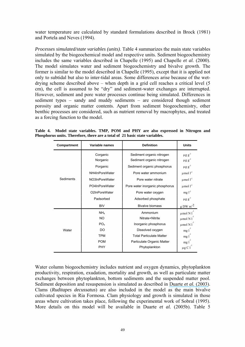
49

water temperature are calculated by standard formulations described in Brock (1981) and Portela and Neves (1994). Processes simulated/state variables (units). Table 4 summarizes the main state variables simulated by the biogeochemical model and respective units. Sediment biogeochemistry includes the same variables described in Chapelle (1995) and Chapelle et al. (2000). The model simulates water and sediment biogeochemistry and bivalve growth. The former is similar to the model described in Chapelle (1995), except that it is applied not only to subtidal but also to inter-tidal areas. Some differences arise because of the wet-drying scheme described above – when depth in a grid cell reaches a critical level (5 cm), the cell is assumed to be “dry” and sediment-water exchanges are interrupted. However, sediment and pore water processes continue being simulated. Differences in sediment types – sandy and muddy sediments – are considered though sediment porosity and organic matter contents. Apart from sediment biogeochemistry, other benthic processes are considered, such as nutrient removal by macrophytes, and treated as a forcing function to the model. Table 4. Model state variables. TMP, POM and PHY are also expressed in Nitrogen and Phosphorus units. Therefore, there are a total of 21 basic state variables.

Compartment Variable names Definition Units

Corganic Sediment organic nitrogen μg g-1

Norganic Sediment organic nitrogen μg g-1

Porganic Sediment organic phosphorus μg g-1

NH4InPoreWater Pore water ammonium μmol l-1

NO3InPoreWater Pore water nitrate μmol l-1

PO4InPoreWater Pore water inorganic phosphorus μmol l-1

O2InPoreWater Pore water oxygen mg l-1

Padsorbed Adsorbed phosphate μg g-1

Sediments

BIV Bivalve biomass g DW m-2

NH4 Ammonium μmol N l-1

NO Nitrate+Nitrite μmol N l

-1

PO4 Inorganic phosphorus μmol N l-1

DO Dissolved oxygen mg l

-1

TPM Total Particulate Matter mg l-1

POM Particulate Organic Matter mg l

-1

Water

PHY Phytoplankton μg C l-1

Water column biogeochemistry includes nutrient and oxygen dynamics, phytoplankton productivity, respiration, exudation, mortality and growth, as well as particulate matter exchanges between phytoplankton, bottom sediments and the suspended matter pool. Sediment deposition and resuspension is simulated as described in Duarte et al. (2003). Clams (Ruditapes decussatus) are also included in the model as the main bivalve cultivated species in Ria Formosa. Clam physiology and growth is simulated in those areas where cultivation takes place, following the experimental work of Sobral (1995). More details on this model will be available in Duarte et al. (2005b). Table 5

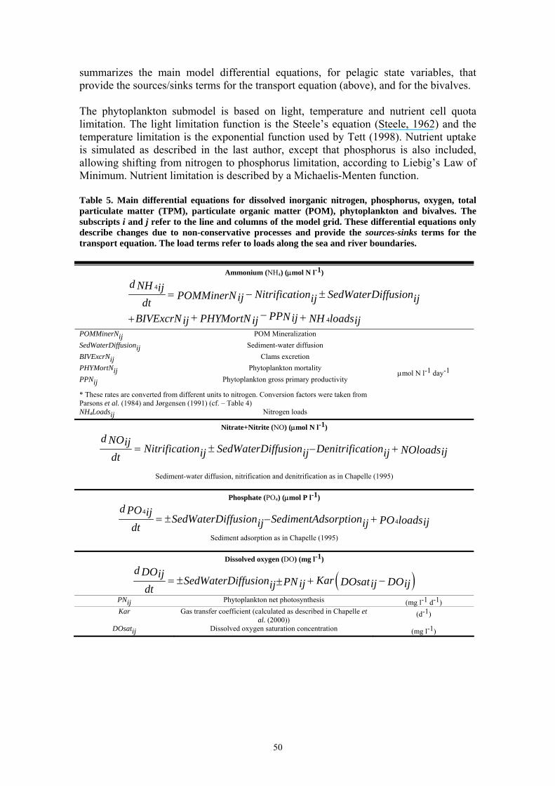
50

summarizes the main model differential equations, for pelagic state variables, that provide the sources/sinks terms for the transport equation (above), and for the bivalves. The phytoplankton submodel is based on light, temperature and nutrient cell quota limitation. The light limitation function is the Steele’s equation (Steele, 1962) and the temperature limitation is the exponential function used by Tett (1998). Nutrient uptake is simulated as described in the last author, except that phosphorus is also included, allowing shifting from nitrogen to phosphorus limitation, according to Liebig’s Law of Minimum. Nutrient limitation is described by a Michaelis-Menten function. Table 5. Main differential equations for dissolved inorganic nitrogen, phosphorus, oxygen, total particulate matter (TPM), particulate organic matter (POM), phytoplankton and bivalves. The subscripts i and j refer to the line and columns of the model grid. These differential equations only describe changes due to non-conservative processes and provide the sources-sinks terms for the transport equation. The load terms refer to loads along the sea and river boundaries.

Ammonium (NH4) (μmol N l-1)

4

4

d NH ij Nitrification SedWaterDiffusionPOMMinerNij ij ijdtPPNijBIVExcrN PHYMortN NH loadsij ij ij

= − ±

−+ ++

POMMinerNij POM Mineralization SedWaterDiffusionij Sediment-water diffusion BIVExcrNij Clams excretion PHYMortNij Phytoplankton mortality PPNij Phytoplankton gross primary productivity

* These rates are converted from different units to nitrogen. Conversion factors were taken from Parsons et al. (1984) and Jørgensen (1991) (cf. – Table 4) NH4Loadsij Nitrogen loads

μmol N l-1 day-1

Nitrate+Nitrite (NO) (μmol N l-1)

d NOij Nitrification SedWaterDiffusion Denitrification NOloadsijij ij ijdt= ± +−

Sediment-water diffusion, nitrification and denitrification as in Chapelle (1995)

Phosphate (PO4) (μmol P l-1)

44

d PO ij SedWaterDiffusion SedimentAdsorption PO loadsijij ijdt= ± +−

Sediment adsorption as in Chapelle (1995)

Dissolved oxygen (DO) (mg l-1)

( )d DOij KarSedWaterDiffusion PN DOsat DOij ij ijijdt= ± + −±

PNij Phytoplankton net photosynthesis (mg l-1 d-1) Kar Gas transfer coefficient (calculated as described in Chapelle et

al. (2000)) (d-1)

DOsatij Dissolved oxygen saturation concentration (mg l-1)

51

Total (TPM) and organic (POM) particulate matter (mg l-1)

dd PHYTOTTPM ij ijTPMDep TPMResus POMMiner TPMLoadsij ij ijijdt dt= − + − + (6)

d dPOM PHYORGij ijPOMDep POMResus POMMiner POMLoadsij ij ijijdt dt= − + − + *

(following Duarte et al. (2003)) TPMDepij TPM Deposition rate TPMResusij TPM Resuspension rate

d PHYTOT ijdt

Net variation on phytoplankton Biomass converted from carbon units

TPMLoadsij TPM loads POMDepij POM Deposition rate POMResusij POM Resuspension rate

d PHYORGijdt

Net variation on phytoplankton Organics

POMMinerij POM mineralization POMLoadsij POM loads

mg l-1 day-1

* - POM and POM fluxes are expressed in POM mass, Carbon, Nitrogen and Phosphorus units

Phytoplankton (μg C l-1)*

( ) -d PHY ij PHYRespPHYGPP PHYExud PHYMortPHY ij ij ij ijijdt

convBIVGb PHYLoadsij BIV ijij

= − − −

+

*For output phytoplankton biomass is converted to Chlorophyll, assuming a Chlrophyll / Carbon ratio of 0.02 (Jørgensen et al., 1991)

Phytoplankton is also expressed in nitrogen and phosphorus units. PHYGPPij Gross primary productivity PHYExudij Exudation rate PHYRespij Respiration rate PHYMortij Mortality rate

Gbij Bivalve grazing rate

day-1

BIVijconvBIV Bivalve biomass converted to carbon

PHYLoadsij Phytoplankton loads

μg C l-1day-1

Bivalves (g DW m-2)

( )d BIV ij BIVRespBIVDens BIVAbsor BIVExcr BIVMortij ij ij ijijdt

BIVSeed BIVHarvij ij

= − − −

+ −

BIVDesnij Density ind. m-2 BIVAbsorij Absorption rate BIVRespij Respiration rate BIVExcrij Excretion rate BIVMortij Mortality rate

g DW ind-1 day-1

BIVSeedij Seeding rate BIVHarvij Harvest rate

g DW m-2 day-1

The model uses simultaneously three currencies: carbon, nitrogen and phosphorus. Therefore, mass transfers between phytoplankton, suspended matter and bottom sediments are “tracked” for these three different elements. It was decided not to assume only one limiting nutrient, to allow for more flexibility in scenario analysis. In fact,

52

some anthropogenic actions that take place in Ria Formosa, such as sediment reworking for mollusc harvest, may have important impacts on sediment biogeochemistry, with important changes in stoichiometry and potential shifts in limiting nutrients (Falcão, personal communication). Input requirements/data preprocessing. The data files needed to run the model were described above (cf. - 3.1.4 RF2D – EcoDynamo). Air temperature, cloud cover and wind velocity time series are necessary with a daily frequency for light intensity and water temperature calculation. Output/postprocessing/scenario analysis. Output data files and graphical outputs using MatLab were described above (cf. - 3.1.4 RF2D – EcoDynamo). Time series for all state variables may be produced for a posteriori calculation of indicators, such as exergy and specific exergy, and also to feedback socio-economic analysis. Limits of application. The biogeochemical model is generally applicable to shallow-water coastal ecosystems. In the case of Ria Formosa, due to the very small time step (see above) there is an important limitation regarding the time span of model simulations. Simulating periods of over two-three months is highly impractical, unless a multi-processing model version is implemented. Accessibility/Portability/Manuals/References. Accessibility: The model is generally available for research purposes. It has been written in C++, but the objects have been compiled as general purpose Dynamic Link Libraries (DLLs), that may be interfaced with Fortran code. In fact, within the scope of the present project some of the EcoDynamo DLLs were already interfaced with COHERENS (Pereira et al., in prep). The model runs on Windows platforms. A report describing the biogeochemical model will be available before the end of June 2005 from http://www.dittyproject.org/reports.asp. 4.1.2. Mar Menor Introduction/Brief description. The Mar Menor lagoon model is a 0D biogeochemical model considering the main processes occurring in the water column and in the sediments, the inflows received from the watershed and the exchange with the Mediterranean sea. The model pays special attention to the inclusion of a jellyfish compartment composed of three species, which are modelled separately. The energy flow through the food web has been described in nitrogen terms, since it was found that this element was the limiting factor for primary production in the Mar Menor lagoon. The model runs on a daily basis, while the simulation time step is kept short enough (less than an hour) to properly simulate all processes considered in the model. The model can perform long term simulations (10-20 years). Figure 11 presents a simplified diagram with the conceptual model of the Mar Menor lagoon.

53

watertemperature

NH4NO3O2

NH4sNO3s O2s

DOM

DOMs

BDs

ZooplanktonPhytoplankton

Rhizostomapulmo

Cotylorhizatuberculata

Aureliaaurita

WatershedExchange

Caulerpaprolifera

Cymodoceanodosa

Figure 11. Simplified diagram of the conceptual model for the Mar Menor lagoon. Processes simulated/State variables (units). The model considers the following fifteen state variables: phytoplankton, zooplankton, Aurelia aurita, Cotylorhiza tuberculata, Rhizostoma pulmo, dissolved organic matter in the water column, dissolved organic matter in the sediment, biodeposits in the sediment, N-NO3 in the water column, N-NO3 in the sediment, N-NH4 in the water column, N-NH4 in the sediment, oxygen in the water column oxygen in the sediment and water temperature. In table 6 are presented the model equations and units for the state variables of the Mar Menor lagoon model. The model includes 5 forcing functions and 54 parameters. The equations of Lancelot (2002) for Aurelia aurita, the native jellyfish species in the Mar Menor, have been adapted to consider only one state variable for phytoplankton and one for zooplankton. The equations from Lancelot (2003) for the omnivorous Pelagia noctiluca were simplified and adapted for the two omnivorous alloctonous jellyfish species Rhizostoma pulmo and Cotylorhiza tuberculata. The modifications are related to some feeding differences between P. noctiluca and the species of the Mar Menor lagoon since, differently from Pelagia noctiluca, neither R. pulmo nor C. tuberculata seem to feed on particulate organic matter. There are additional differences in the case of C. tuberculata, since this species has endosymbiotic zooxantelas which are capable of directly use the dissolved nutrients (nitrate and ammonium in the water column). The endosymbiotic dinoflagellates of Cotylorhiza tuberculata play a key role in the proliferation of this scyphomedusan through the direct assimilation of the dissolved nutrients in the water column and the translocation of the carbon fixed to the host. The picophytoplancton equations from Chapelle et al. (2000) were used to simulate the nutrients assimilation by the endosymbiotic dinoflagellates of C. tuberculata.

54

Table 6. Model equations and units of the state variables in the Mar Menor lagoon model.

Inputs requirements/Data preprocessing. The lagoon model has the following five forcing functions: biomass of Caulerpa prolifera; Cymodocea nodosa, NO3 inputs from watershed, NO3 inputs from the Mediterranean sea, NO3 outputs to the Mediterranean sea. Forcing functions can be directly loaded into the Mar Menor model as ASCII data series. Output/postprocessing/scenario analysis. Simulation results for all variables (state, flow and intermediate variables) are possible. Model outputs may be obtained as tables, figures and ASCII data series The software allows several quantitative and graphical analysis of simulation results, automatic calibration of specified parameters and sensitivity analysis through Montecarlo simulation. The simulation of built-in scenarios is also possible. Limits of application. The model has been calibrated using 1996-1997 data. Additional data are required to carry out an extended calibration of the model. Accessibility/Portability/Manuals/References. The presented model has been largely based on Chapelle et al. (2000) and Plus et al. (2003) for the geochemical cycles and a majority of the biological part. The jellyfish submodel has been adapted from Lancelot et al. (2002), whereas the sediment and oxygen submodels, as well as the nitrogen exchange at the seawater-sediment interface, have been adapted from Chapelle (1995).

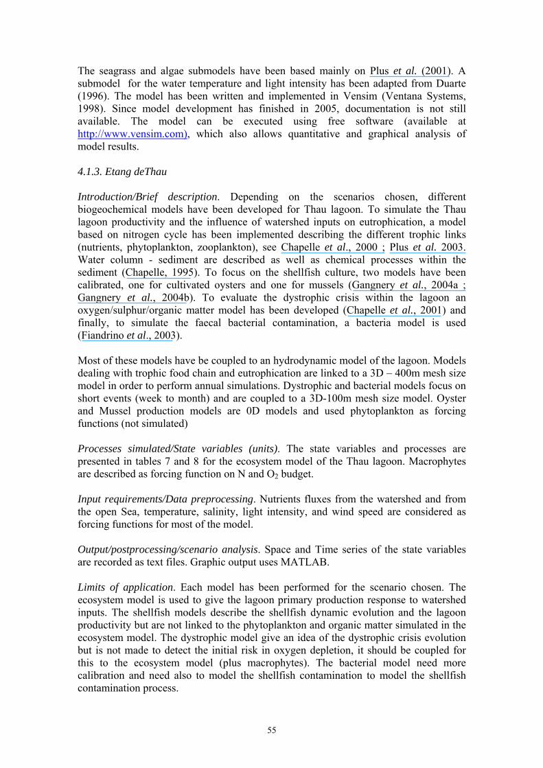
55

The seagrass and algae submodels have been based mainly on Plus et al. (2001). A submodel for the water temperature and light intensity has been adapted from Duarte (1996). The model has been written and implemented in Vensim (Ventana Systems, 1998). Since model development has finished in 2005, documentation is not still available. The model can be executed using free software (available at http://www.vensim.com), which also allows quantitative and graphical analysis of model results. 4.1.3. Etang deThau Introduction/Brief description. Depending on the scenarios chosen, different biogeochemical models have been developed for Thau lagoon. To simulate the Thau lagoon productivity and the influence of watershed inputs on eutrophication, a model based on nitrogen cycle has been implemented describing the different trophic links (nutrients, phytoplankton, zooplankton), see Chapelle et al., 2000 ; Plus et al. 2003. Water column - sediment are described as well as chemical processes within the sediment (Chapelle, 1995). To focus on the shellfish culture, two models have been calibrated, one for cultivated oysters and one for mussels (Gangnery et al., 2004a ; Gangnery et al., 2004b). To evaluate the dystrophic crisis within the lagoon an oxygen/sulphur/organic matter model has been developed (Chapelle et al., 2001) and finally, to simulate the faecal bacterial contamination, a bacteria model is used (Fiandrino et al., 2003). Most of these models have be coupled to an hydrodynamic model of the lagoon. Models dealing with trophic food chain and eutrophication are linked to a 3D – 400m mesh size model in order to perform annual simulations. Dystrophic and bacterial models focus on short events (week to month) and are coupled to a 3D-100m mesh size model. Oyster and Mussel production models are 0D models and used phytoplankton as forcing functions (not simulated) Processes simulated/State variables (units). The state variables and processes are presented in tables 7 and 8 for the ecosystem model of the Thau lagoon. Macrophytes are described as forcing function on N and O2 budget. Input requirements/Data preprocessing. Nutrients fluxes from the watershed and from the open Sea, temperature, salinity, light intensity, and wind speed are considered as forcing functions for most of the model. Output/postprocessing/scenario analysis. Space and Time series of the state variables are recorded as text files. Graphic output uses MATLAB. Limits of application. Each model has been performed for the scenario chosen. The ecosystem model is used to give the lagoon primary production response to watershed inputs. The shellfish models describe the shellfish dynamic evolution and the lagoon productivity but are not linked to the phytoplankton and organic matter simulated in the ecosystem model. The dystrophic model give an idea of the dystrophic crisis evolution but is not made to detect the initial risk in oxygen depletion, it should be coupled for this to the ecosystem model (plus macrophytes). The bacterial model need more calibration and need also to model the shellfish contamination to model the shellfish contamination process.

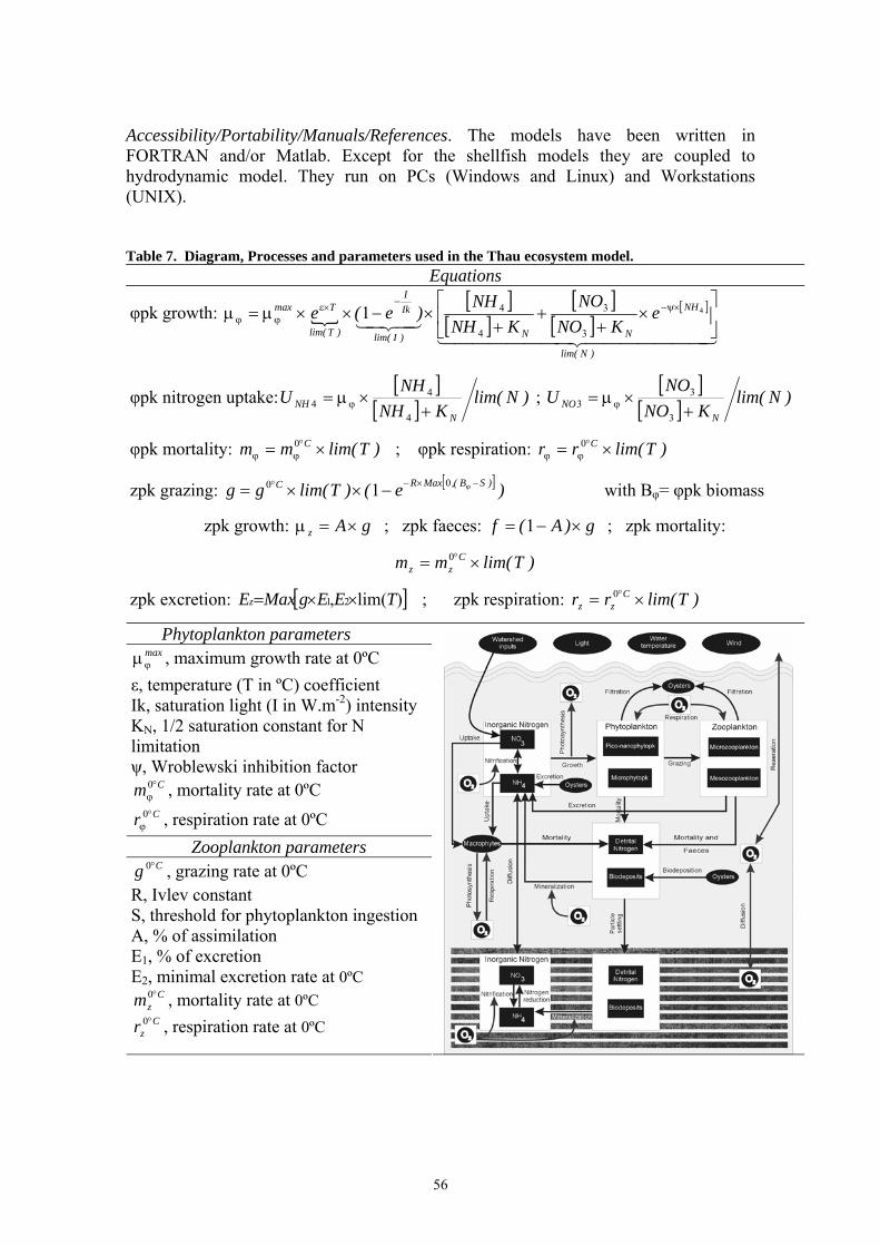
56

Accessibility/Portability/Manuals/References. The models have been written in FORTRAN and/or Matlab. Except for the shellfish models they are coupled to hydrodynamic model. They run on PCs (Windows and Linux) and Workstations (UNIX). Table 7. Diagram, Processes and parameters used in the Thau ecosystem model.

Equations

φpk growth: {[ ]

[ ][ ]

[ ][ ]

4444444 34444444 2143421

)Nlim(

NH

NN)Ilim(

IkI

)Tlim(

Tmax eKNO

NOKNH

NH)e(e ⎥⎦

⎤⎢⎣

⎡×

++

+×−××μ=μ ×ψ−−×ε

ϕϕ4

3

3

4

41

φpk nitrogen uptake:[ ]

[ ] )Nlim(KNH

NHUN

NH +×μ= ϕ

4

44 ;

[ ][ ] )Nlim(

KNONO

UN

NO +×μ= ϕ

3

33

φpk mortality: )Tlim(mm C ×= °ϕϕ0 ; φpk respiration: )Tlim(rr C ×= °

ϕϕ0

zpk grazing: [ ] )e()Tlim(gg )SB(,MaxRC −×−° ϕ−××= 00 1 with Bφ= φpk biomass

zpk growth: gAz ×=μ ; zpk faeces: g)A(f ×−= 1 ; zpk mortality:

)Tlim(mm Czz ×= °0

zpk excretion: [ ])lim(, 21 TEEgMaxEz ××= ; zpk respiration: )Tlim(rr Czz ×= °0

Phytoplankton parameters maxϕμ , maximum growth rate at 0ºC

ε, temperature (T in ºC) coefficient Ik, saturation light (I in W.m-2) intensity KN, 1/2 saturation constant for N limitation ψ, Wroblewski inhibition factor

Cm °ϕ0 , mortality rate at 0ºC Cr °

ϕ0 , respiration rate at 0ºC

Zooplankton parameters Cg °0 , grazing rate at 0ºC

R, Ivlev constant S, threshold for phytoplankton ingestion A, % of assimilation E1, % of excretion E2, minimal excretion rate at 0ºC

Czm °0 , mortality rate at 0ºC C

zr °0 , respiration rate at 0ºC

57

Table 8. State variables and processes in the different Thau models. Dystrophic model

Variable name

Definition Units

MO Organic matter mmol N/m3 O2 Dissolved oxygen g O2/m

3 S2- Sulfur mmol /m3

Aerobic mineralisation : miner= tauxmin*exp(0,07*temp)*[MO]* [O2]/([ O2]+KO2)

Anaerobic mineralisation : minera= tauxmina*exp(0,7*temp)*[MO]*(1-[O2]/([ O2]+KO2))

Sulfur oxydation : tauxoxys*exp(0,7*temp)*limo2*[S2-]

Sea-air exchanges : Oreaeration = (0.641+0.0256*[(wind/0.447)2)/depth ]*(osat - [O2])

Sreaeration = cteair*[S2-]

Faecal Bacterial model The work by Martin et al. [Martin et al. 1998], which served as a basis for the biological model used here, supposes that viable cultivable bacteria (VCB) can modulate to a physiological state where they are viable but non-cultivable (VNCB) when the environmental conditions become unfavourable (nutrient deficit, salinity gradient, insolation…). The model separates each of these two categories of bacteria into two size classes, those of more than or less than 3 μm. The first group, qualified as free, do not settle, while the second group, attached, fall through the water column.

Enterobacterial flow

Hydrodynamique modelMARS-3D

Biological module fateof enterobacteria in the watercolumn

Environmentalstress

- substrate deficency- hyperosmotic shock- insolation- hypothermic shock

VCB : Viablecultivable bacteria(mesurable)VNCB Viablenon cultivable bacteriaVCB

free/attachedVNCB

free/attached

Lysedbacteria

Variable

name Definition Units (inputs of the model)

In water column

VCB-free free viable cultivable bacteria

cell/100ml VCB-

attached attached viable cultivable bacteria

VNCB-free

free viable non-cultivable bacteria

VNCB-attached

attached viable non-cultivable bacteria

In shellfish VCB-

attached attached viable cultivable bacteria cells /100gr-1 of wet weight shellfish flesh

VNCB-attached

attached viable non-cultivable bacteria

In sediment

VCB-attached

attached viable cultivable bacteria (Cell/m2)

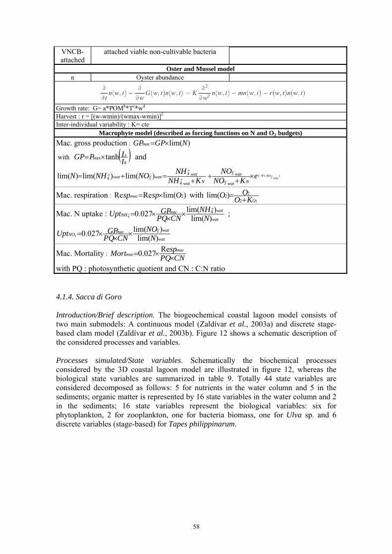
58

VNCB-attached

attached viable non-cultivable bacteria

Oster and Mussel model n Oyster abundance

Growth rate: G= a*POMb*Tc*wd Harvest : r = [(w-wmin)/(wmax-wmin)]2 Inter-individual variability : K= cte

Macrophyte model (described as forcing functions on N and O2 budgets) Mac. gross production : )lim(NGPGPmac ×=

with ( ) tanhmaxkz

IIPGP ×= and

)3(

3

3

4

434 )lim()lim()lim( wat

NOeKNONO

KNHNHNONHN

Nwat

wat

Nwat

watwatwat −×Ψ−×+++=+=−

−

+

+−+

Mac. respiration : )lim(ReRe 2Ospspmac ×= with 22

22)lim(OKO

OO +=

Mac. N uptake : wat

watmacNH NNH

CNPQGPUpt )lim(

)lim(027.0 44

+×××=+ ;

wat

watmacNO NNO

CNPQGPUpt )lim(

)lim(027.0 33

−×××=−

Mac. Mortality : CNPQspMort mac

mac ××= Re027.0

with PQ : photosynthetic quotient and CN : C:N ratio

4.1.4. Sacca di Goro Introduction/Brief description. The biogeochemical coastal lagoon model consists of two main submodels: A continuous model (Zaldívar et al., 2003a) and discrete stage-based clam model (Zaldívar et al., 2003b). Figure 12 shows a schematic description of the considered processes and variables. Processes simulated/State variables. Schematically the biochemical processes considered by the 3D coastal lagoon model are illustrated in figure 12, whereas the biological state variables are summarized in table 9. Totally 44 state variables are considered decomposed as follows: 5 for nutrients in the water column and 5 in the sediments; organic matter is represented by 16 state variables in the water column and 2 in the sediments; 16 state variables represent the biological variables: six for phytoplankton, 2 for zooplankton, one for bacteria biomass, one for Ulva sp. and 6 discrete variables (stage-based) for Tapes philippinarum.

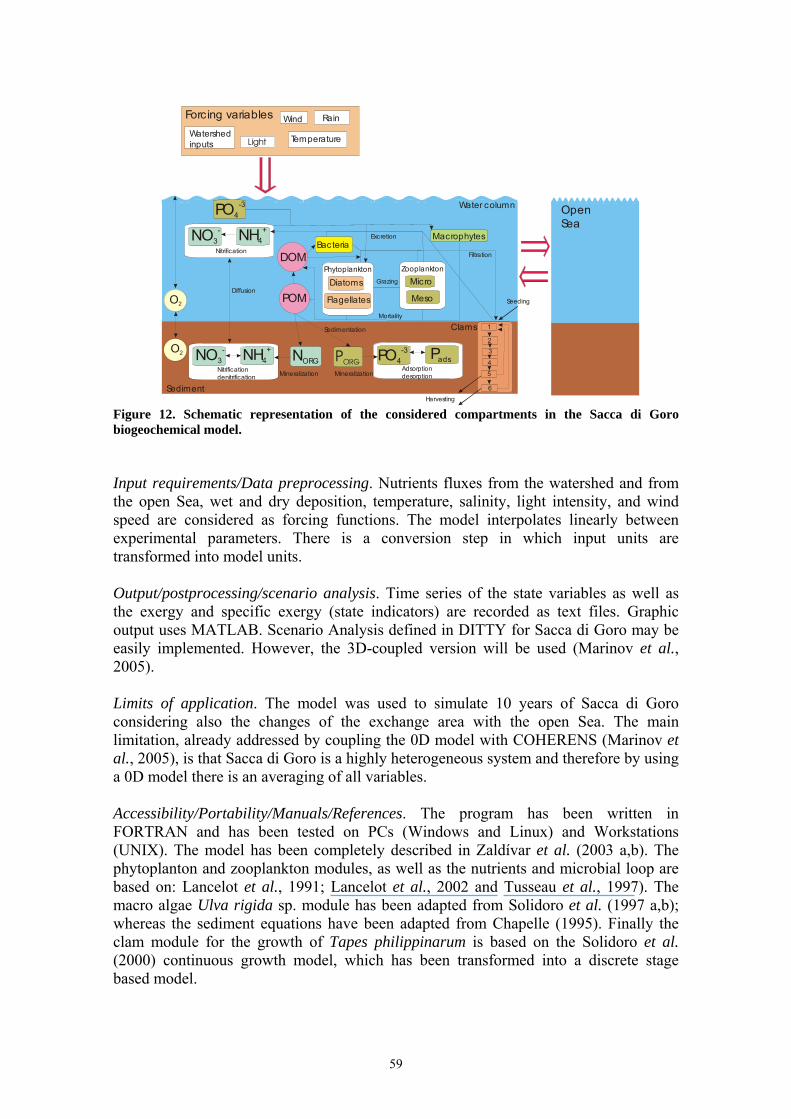
59

Figure 12. Schematic representation of the considered compartments in the Sacca di Goro biogeochemical model. Input requirements/Data preprocessing. Nutrients fluxes from the watershed and from the open Sea, wet and dry deposition, temperature, salinity, light intensity, and wind speed are considered as forcing functions. The model interpolates linearly between experimental parameters. There is a conversion step in which input units are transformed into model units. Output/postprocessing/scenario analysis. Time series of the state variables as well as the exergy and specific exergy (state indicators) are recorded as text files. Graphic output uses MATLAB. Scenario Analysis defined in DITTY for Sacca di Goro may be easily implemented. However, the 3D-coupled version will be used (Marinov et al., 2005). Limits of application. The model was used to simulate 10 years of Sacca di Goro considering also the changes of the exchange area with the open Sea. The main limitation, already addressed by coupling the 0D model with COHERENS (Marinov et al., 2005), is that Sacca di Goro is a highly heterogeneous system and therefore by using a 0D model there is an averaging of all variables. Accessibility/Portability/Manuals/References. The program has been written in FORTRAN and has been tested on PCs (Windows and Linux) and Workstations (UNIX). The model has been completely described in Zaldívar et al. (2003 a,b). The phytoplanton and zooplankton modules, as well as the nutrients and microbial loop are based on: Lancelot et al., 1991; Lancelot et al., 2002 and Tusseau et al., 1997). The macro algae Ulva rigida sp. module has been adapted from Solidoro et al. (1997 a,b); whereas the sediment equations have been adapted from Chapelle (1995). Finally the clam module for the growth of Tapes philippinarum is based on the Solidoro et al. (2000) continuous growth model, which has been transformed into a discrete stage based model.

Forcing variables Wind

TemperatureWatershedinputs

Rain

Sediment

O2

O2

Water column

Diatoms

Flagellates

PhytoplanktonMicro

Meso

Zooplankton

Macrophytes

NO3- NH4

+

Clams

Nitrificationdenitrification

NORG PO4-3 PadsAdsorptiondesorptionMineralization Mineralization

NO3- NH4

+

Nitrification

Grazing

FiltrationDOM

POM

Bacteria

PO4-3

Excretion

Mortality

OpenSea

Diffusion

Sedimentation

Seeding

Harvesting

1

2

3

4

5

6

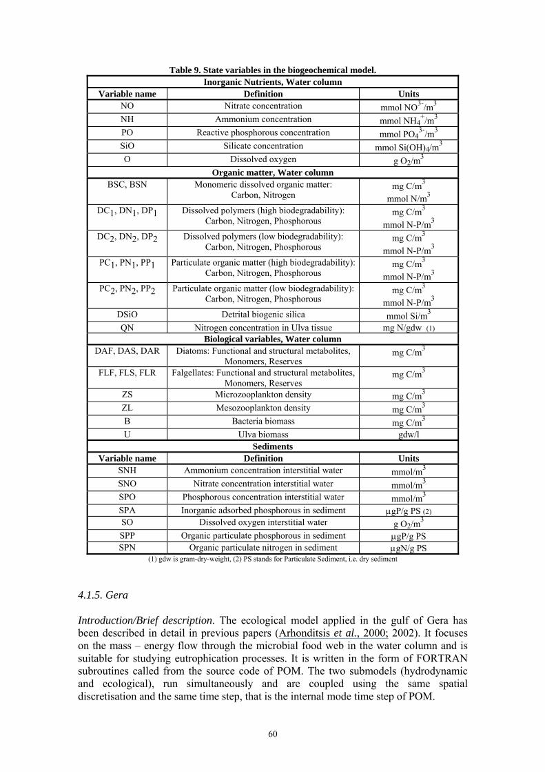
60

Table 9. State variables in the biogeochemical model. Inorganic Nutrients, Water column

Variable name Definition Units NO Nitrate concentration mmol NO3-/m3 NH Ammonium concentration mmol NH4

+/m3 PO Reactive phosphorous concentration mmol PO4

3-/m3 SiO Silicate concentration mmol Si(OH)4/m3 O Dissolved oxygen g O2/m3

Organic matter, Water column BSC, BSN Monomeric dissolved organic matter:

Carbon, Nitrogen mg C/m3

mmol N/m3 DC1, DN1, DP1 Dissolved polymers (high biodegradability):

Carbon, Nitrogen, Phosphorous mg C/m3

mmol N-P/m3 DC2, DN2, DP2 Dissolved polymers (low biodegradability):

Carbon, Nitrogen, Phosphorous mg C/m3

mmol N-P/m3 PC1, PN1, PP1 Particulate organic matter (high biodegradability):

Carbon, Nitrogen, Phosphorous mg C/m3

mmol N-P/m3 PC2, PN2, PP2 Particulate organic matter (low biodegradability):

Carbon, Nitrogen, Phosphorous mg C/m3

mmol N-P/m3 DSiO Detrital biogenic silica mmol Si/m3 QN Nitrogen concentration in Ulva tissue mg N/gdw (1)

Biological variables, Water column DAF, DAS, DAR Diatoms: Functional and structural metabolites,

Monomers, Reserves mg C/m3

FLF, FLS, FLR Falgellates: Functional and structural metabolites, Monomers, Reserves

mg C/m3

ZS Microzooplankton density mg C/m3 ZL Mesozooplankton density mg C/m3 B Bacteria biomass mg C/m3 U Ulva biomass gdw/l

Sediments Variable name Definition Units

SNH Ammonium concentration interstitial water mmol/m3 SNO Nitrate concentration interstitial water mmol/m3 SPO Phosphorous concentration interstitial water mmol/m3 SPA Inorganic adsorbed phosphorous in sediment μgP/g PS (2) SO Dissolved oxygen interstitial water g O2/m3 SPP Organic particulate phosphorous in sediment μgP/g PS SPN Organic particulate nitrogen in sediment μgN/g PS

(1) gdw is gram-dry-weight, (2) PS stands for Particulate Sediment, i.e. dry sediment 4.1.5. Gera Introduction/Brief description. The ecological model applied in the gulf of Gera has been described in detail in previous papers (Arhonditsis et al., 2000; 2002). It focuses on the mass – energy flow through the microbial food web in the water column and is suitable for studying eutrophication processes. It is written in the form of FORTRAN subroutines called from the source code of POM. The two submodels (hydrodynamic and ecological), run simultaneously and are coupled using the same spatial discretisation and the same time step, that is the internal mode time step of POM.

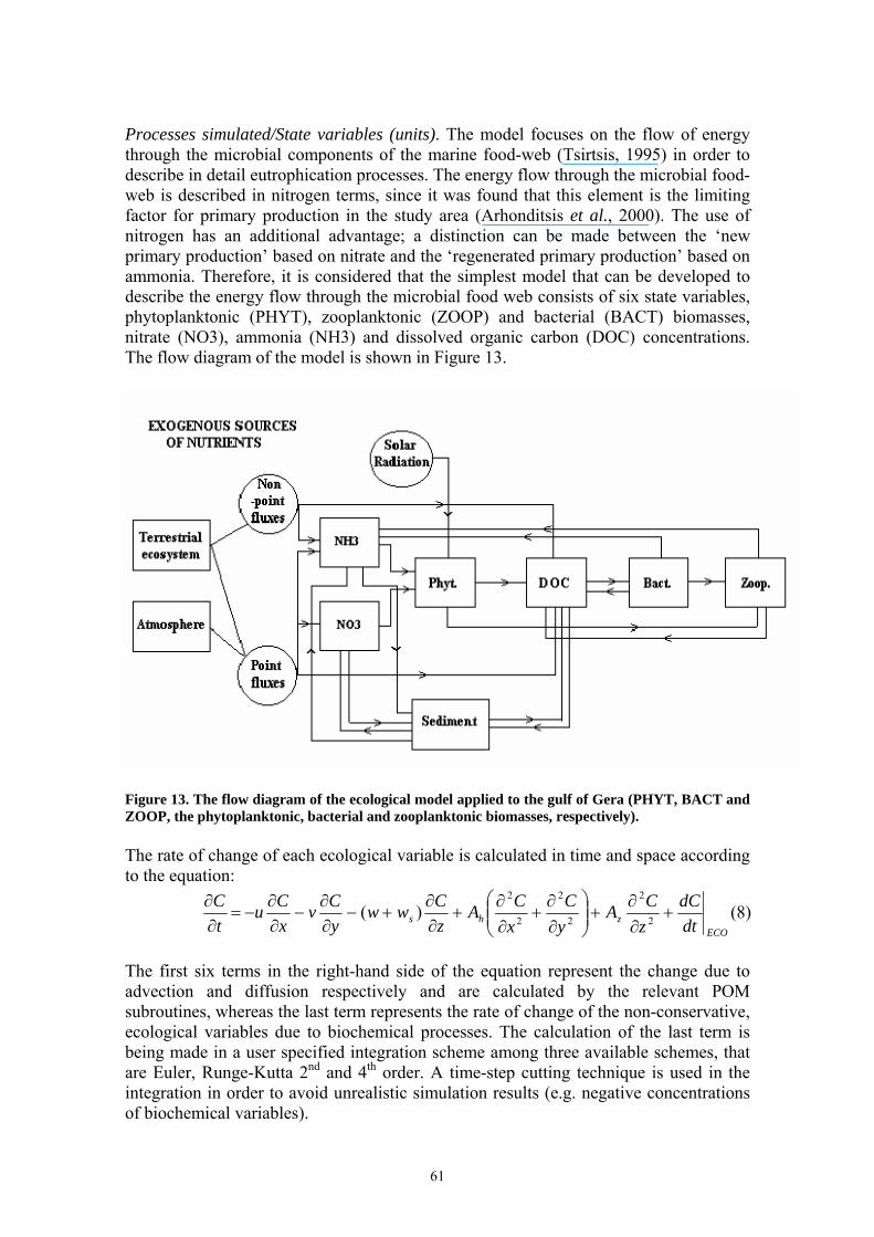
61

Processes simulated/State variables (units). The model focuses on the flow of energy through the microbial components of the marine food-web (Tsirtsis, 1995) in order to describe in detail eutrophication processes. The energy flow through the microbial food-web is described in nitrogen terms, since it was found that this element is the limiting factor for primary production in the study area (Arhonditsis et al., 2000). The use of nitrogen has an additional advantage; a distinction can be made between the ‘new primary production’ based on nitrate and the ‘regenerated primary production’ based on ammonia. Therefore, it is considered that the simplest model that can be developed to describe the energy flow through the microbial food web consists of six state variables, phytoplanktonic (PHYT), zooplanktonic (ZOOP) and bacterial (BACT) biomasses, nitrate (NO3), ammonia (NH3) and dissolved organic carbon (DOC) concentrations. The flow diagram of the model is shown in Figure 13.

Figure 13. The flow diagram of the ecological model applied to the gulf of Gera (PHYT, BACT and ZOOP, the phytoplanktonic, bacterial and zooplanktonic biomasses, respectively).

The rate of change of each ecological variable is calculated in time and space according to the equation:

ECO

zhs dtdC

zCA

yC

xCA

zCww

yCv

xCu

tC

+∂∂

+⎟⎟⎠

⎞⎜⎜⎝

⎛∂∂

+∂∂

+∂∂

+−∂∂

−∂∂

−=∂∂

2

2

2

2

2

2

)( (8)

The first six terms in the right-hand side of the equation represent the change due to advection and diffusion respectively and are calculated by the relevant POM subroutines, whereas the last term represents the rate of change of the non-conservative, ecological variables due to biochemical processes. The calculation of the last term is being made in a user specified integration scheme among three available schemes, that are Euler, Runge-Kutta 2nd and 4th order. A time-step cutting technique is used in the integration in order to avoid unrealistic simulation results (e.g. negative concentrations of biochemical variables).

62

Input requirements/Data preprocessing. The ecological model is called as a subroutine from the POM code and uses the same temporal and spatial resolution, that has been described before, for POM. Therefore, initial and boundary conditions must be defined for the six state variables. Initial values are defined on a 3-d grid through spatial interpolation based on existing data from a network of seven stations spaced out in the study area. Boundary conditions are also defined for the open boundaries for each time step using spatial and temporal interpolation. Two boundaries exist in the current application. Sea surface and the vertical plane separating the gulf from the open sea. The nutrient and organic matter fluxes from the watershed are incorporated through the distributions of these materials at the sea surface. Output/postprocessing/scenario analysis. The output of the model is in the form of matrices (text files). The visualization of the results is being carried out with MATLAB. Scenario analyses can be carried out by altering the inputs from the watershed model. Limits of application. The model can be applied in order to test scientific questions related to the dynamics of plankton and its relationships with environmental factors. There are no limitations, provided that information is available to define initial and boundary conditions. Accessibility/Portability/Manuals/References. The model has been written in Standard FORTRAN 77 and can be run on any machine (PC, Linux, Unix) running FORTRAN. Methodological details about the model and the coupling procedure are available (Arhonditsis et al., 2000; 2002; Kolovoyiannis et al., 2005). 4.2. Summarizing tables

63

Table 10. Main characteristic of the biogeochemical models used.

1. General information Menor lagoon Thau lagoon Goro Lagoon Ria Formosa Gera gulf

1.1 State variables - Water column

10: phytoplankton, zooplankton, Aurelia aurita, Cotylorhyza tuberculata, Rhyzostoma pulmo, DOM, N-NO3, N-NH4, O2, water temperature

8: Phytoplankton (2 groups), zooplankton (2 groups), DOM, biodeposits, N-NO3, N-NH4, O2;

31: inorganic matter (N-NO3, N-NH4, phosphorus, silica) and O2; organic matter (monomeric C and N, dissolved polymers -C,N,P- of high and low biodegrability, particulate C,N,P of high and low biodegrability; detrital silica and N in Ulva tissue; biological (phytoplankton, metabolites, monomers, reserves of diatoms and flagellates, zooplankton (micro and meso), bacteria, Ulva sp.)

7: Ammonium, N-NO3+ N-NO2, Inorganic phosphorus, DO, Total Particulate Matter, Particulate Organic Matter, Phytoplankton

6: N-NO3, N-NH4, DOC, Phytoplankton, Zooplankton, Bacteria

- Sediments

5: DOMs, biodeposits, N-NO3s, N-NH4s, O2s

5: DOMs, biodeposits, N-NO3s, N-NH4s, O2s

7: inorganic matter in interstitial water (N-NO3, N-NH4, P, O2), adsorbed inorganic P and particulate organic N and P; bivalves (6 discrete variables = 6 classes of shellfish development

11: Organic C, Organic N, Organic P, Pore water ammonium, Pore water nitrate, Pore water inorganic P, Pore water O, Adsorbed phosphate, Bivalve biomass, Zostera biomass and numerical density

1.2 Processes advection, diffusion, nitrification, denitrification, mineralization, adsorption, desorption, sedimentation, respiration, sea-surface exchange, nutrients uptake, growth, mortality, photosynthesis, lysis, grazing, egestion, storage, catabolism, exudation, filtration, seeding, harvesting.

sediment water exchanges of nutrients and oxygen, deposition and resuspension of detritus and algal cells, mineralization, nitrification, denitrification, phosphorus adsorption-desorption, air-water oxygen exchanges, bivalve and zostera physiology and population dynamics

nutrient uptake, Phytoplankton growth, mortality and exudation, Zooplankton grazing, DOC production, Bacterial growth and mortality, Bacterial mineralization

1.3 Time scale day - year day - year hour - day - month - year hour-day-month day - year

64

1.4 Forcing functions Caulerpa prolifera, Cymodocea nodosa, NO3 watershed input, NO3 Mediterranean input, NO3 output to Mediterranean

nutrients fluxes from watershed and open sea, wet and dry deposition, surface and bottom exchange, heat flux, salinity, light intensity and wind speed.

air temperature, wind speed, solar radiation, river flows and loads, sea boundary conditions and tidal height at sea boundaries

solar radiation, Terrestrial inputs, Water circulation

1.5 Software Vensim

Runge Kutta 4 Fortran, Mat lab Elise, Mars3D

Runge-Kutta 4 Remark: the coupled model uses numerical techniques of COHERENS model. FORTRAN and MATLAB for Windows and UNIX

Object oriented C++, MATLAB

Runge-Kutta 4 FORTRAN, MATLAB

1.6 Hardware PC PC and/or Workstation PC PC, Unix 1.7 Stand alone/coupling - Coupling procedure

stand alone yes the 3D model has been coupled with hydrodynamic part of COHERENS and with the Burano-Volano watershed model.

Embedded in 2D; the model may run coupled with hydrodynamics or using hydrodynamic simulations as forcing for the transport processes

coupling with POM

1.8 Calibration/Validation - Methodology

preliminary calibration /the software includes specific modules for structural validation visual and automatic (the software includes calibration and optimization modules) Montecarlo simulation

yes, visual fitting yes based on visual comparisons with real data and a posteriori statistical tests

preliminary calibration of a 0-d version

1.9 Sensitivity Analysis The 0D biogeochemical model was checked especially about sensitivity of optimal and interval temperature parameters for different species.

sensitivity to model parameters, by changing their values in a parameter file

visual and automatic

1.10 Limitations SG is a highly heterogeneous system therefore using of a 0D model with averaged variables is not suitable for this case and a 3D version has been developed. Further bettering of data about watershed input and open sea exchange will give superior results.

large computing time due to the small time step required by the wet-drying scheme of the model

1.11 Public/Proprietary proprietary software. Freeware model code is freely distributed for proprietary software, proprietary software

65

available for model execution scientific purposes. available for research purposes upon request

1.12 References Chapelle A., Plus M., Fiandrino A., Bacher C. Ifremer

Zaldivar et al., 2003 a; Zaldivar et al., 2003 b; Marinov et al., 2005

Duarte et al., 2005a; 2005b

Tsirtsis, 1995; Arhonditsis et al., 2000; 2002

1.13 Contact point Julia Martínez. Univ. Murcia. J.M. Zaldivar, EC, JRC, IES, Italy jose.zaldivar-comenges@jrc.it

P. Duarte, UFP, Portugal

George Tsirtsis, Univ. of the Aegean, Greece

2. Data requirement

2.1 Forcing functions - 2.1.1.Meteorological variables

- Frequency

none

temperature, wind speed and direction, solar intensity

wind (speed and direction), air temperature, humidity, cloud covering, precipitation hourly frequency

air temperature, wind speed and solar radiation

solar radiation on a daily basis, temperature and velocity fields from POM

- 2.1.2. External inputs - Watershed - Open Sea - Others

NO3 input NO3 input and output to Mediterranean biomass of Caulerpa prolifera, biomass of Cymodocea nodosa

NH4, NO3 input NH4, NO3 , O2, phytoplankton by data interpolation

discharge, temperature, salinity, nitrates, ammonium, phosphate, total P, silica, oxygen; temperature, salinity, oxygen, DIN, phosphate, total N, total P, chl a; PAR, atmospheric dry and wet deposition (airshed nutrient flux)

watershed: flows and loads for all water columns state variables described above; open sea: concentrations for all water columns state variables at the sea boundaries; others: flows and loads for all water columns state variables, from Waste Water Treatment Plants

NO3, NH3, DOC NO3, NH3, DOC exchange with the open sea

2.2 Calibration/validation - Water column - Sediments

yes The biogeochemical part of 3D lagoon model was calibrated/verified only by visual fitting (Marinov et al., 2005).

ongoing

3. Output

3.1 State variables 3.2 Flows

all 66 flows affecting the 15 state variables

all state variables + accessory variables which can be flows - Time series

standard output of all state variables or user-defined output. Time series

all state variables + accessory variables flows affecting state variables

specified above Specified above

66

3.3 Output Format 3.4 Graphics

Data series in ASCII and xls yes

yes

ASCII and BINARY Graphical interface is not directly included in the code but output information can be visualized by MATLAB, EXCEL or other software

ASCII and Hierarchical data format files MatLab graphics

Matrices in text files MATLAB

4. Processes in Water Column

4.1 Nutrients full nitrogen cycle including NH4 diffusion, NO3 diffusion, NO3 uptake, NH4 uptake

full nitrogen cycle including NH4 diffusion, NO3 diffusion, NO3 uptake, NH4 uptake

N, P and Si cycles N,P cycles, mineralization, denitrification, nitrification, NH4 diffusion, NO3 diffusion, NO3 uptake, NH4 uptake

full nitrogen cycle including NH4 diffusion, NO3 diffusion, NO3 uptake, NH4 uptake

4.2.Oxygen - mineralization - nitrification - denitrification - diffusion - uptake - ammonification

O2 diffusion Exchange at sea surface O2 used in the mineralization process

O2 diffusion Exchange at sea surface O2 used in the mineralization process Organisms Respiration

Yes Yes Yes (phytoplankton - Ulva) Yes (phytoplankton - Ulva) Yes (zooplankton - bacteria - shellfish) Yes

O2 diffusion; exchange at sea surface, O2 used in the mineralization process, organisms respiration

4.3 Organic matter /microbial loop - Organic matter production - Organic matter degradation - Bacteria growth - Bacteria respiration - Bacteria degradation

production and degradation of dissolved and particulate organic matter

production of POM by mortality and faeces. mineralisation function of O2 . No bacterial loop

monomeric organic matter (C,N), DOM and POM (C,N,P) of low and high degradability. Yes Yes Yes Yes Yes Yes

Production of POM by mortality and faeces. Mineralisation function of O2 . No bacterial loop

production of dissolved organic matter degradation of dissolved organic matter bacterial loop

4.4 Planktonic components - Photosynthesis - Phytopklankton growth - Phytoplankton respiration - Phytoplankton degradation - Phytoplankton sed. rate - Zooplankton grazing - Zooplankton respiration - Zooplankton degradation

yes yes yes yes no yes yes yes

yes yes yes yes yes yes yes yes

Yes Yes Yes Yes Yes Yes Yes Yes

yes yes yes yes yes no no no

yes yes yes yes no yes yes yes

4.5 Macrophytes Biomass as forcing input Biomass as forcing input Yes

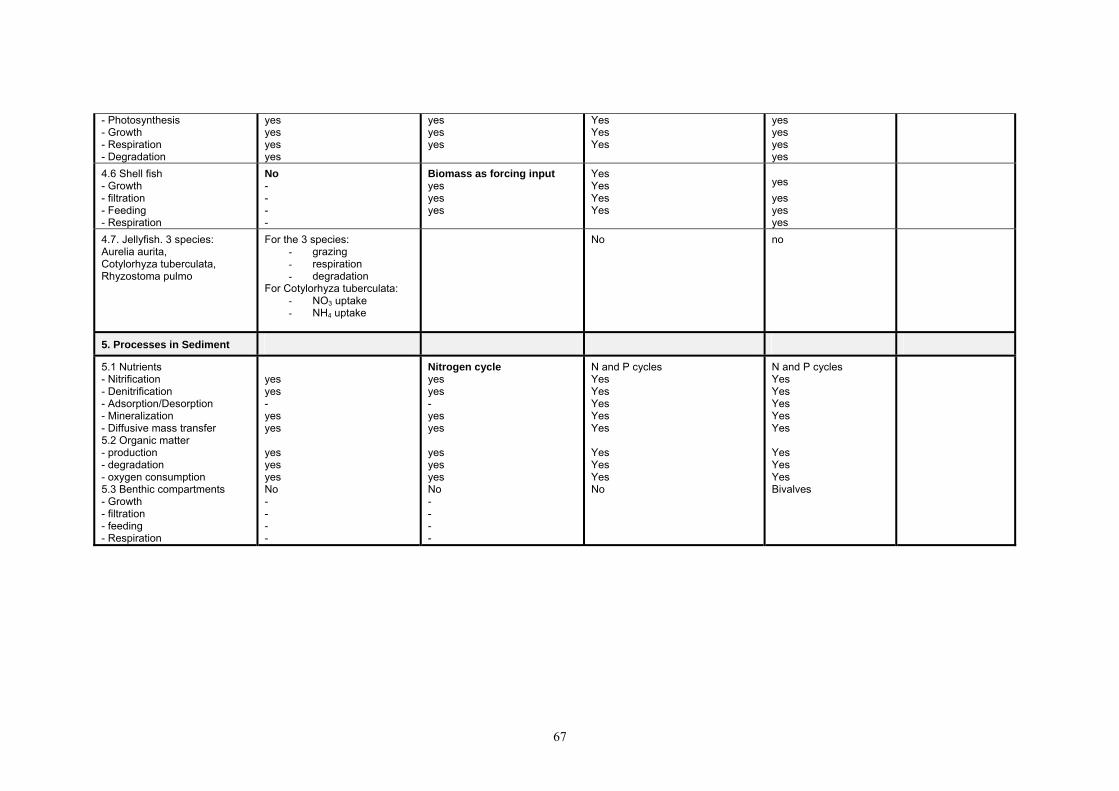
67

- Photosynthesis - Growth - Respiration - Degradation

yes yes yes yes

yes yes yes

Yes Yes Yes

yes yes yes yes

4.6 Shell fish - Growth - filtration - Feeding - Respiration

No - - - -

Biomass as forcing input yes yes yes

Yes Yes Yes Yes

yes yes yes yes

4.7. Jellyfish. 3 species: Aurelia aurita, Cotylorhyza tuberculata, Rhyzostoma pulmo

For the 3 species: - grazing - respiration - degradation

For Cotylorhyza tuberculata: - NO3 uptake - NH4 uptake

No no

5. Processes in Sediment

5.1 Nutrients - Nitrification - Denitrification - Adsorption/Desorption - Mineralization - Diffusive mass transfer

yes yes - yes yes

Nitrogen cycle yes yes - yes yes

N and P cycles Yes Yes Yes Yes Yes

N and P cycles Yes Yes Yes Yes Yes

5.2 Organic matter - production - degradation - oxygen consumption

yes yes yes

yes yes yes

Yes Yes Yes

Yes Yes Yes

5.3 Benthic compartments - Growth - filtration - feeding - Respiration

No - - - -

No - - - -

No Bivalves

68

4.2. Model intercomparison analysis Intercomparison for the models presented in the previous pages will be limited to the processes writing as it is described in the 4.1 section. No comparison based on statistical analysis of results can be performed, as each lagoon has been modelled with a different biogeochemical model, in turn coupled to a different hydrodynamics model. A quantitative intercomparison process would require testing of the different models, all coupled to the same hydrodynamic model, in the same lagoon. However, such endeavour is difficult to achieve, as several possibilities exist and as each model is parameterized for the specific area of concern. Biological models are defined for each case study in function of the model objectives, i.e. fish and/or shellfish farming, macroalgae blooms, dynamics of bacteria of sanitary concern, jellyfish. Thus, even when the structure is very similar, models are different from one site to another and have specially tailored biogeochemical writing for the food chain, differing from one case to the next in the complexity chosen and the knowledge of the processes described. However, in all cases a basic representation of the food chain related to nutrient cycling can be found. The Goro and Ria Formosa models describe the N and P cycles, as both elements could be involved in primary production limitation; Mar Menor, Thau and Gulf of Gera models only consider the N cycle, as this is the limiting factor for primary production. The latter is modelled with the state variable phytoplankton, which can be a general variable (Mar Menor, Ria Formosa, Gera) or composed of 2 functional groups (piconanoplankton and microplankton for Thau, flagellates and diatoms for Goro). Splitting the phytoplankton in different groups allows to reproduce different features of primary production, such as the regenerated production due to the small algae in Thau, the new production due to microplankton as diatoms and the impact of silicium on primary production needed by the diatoms in Goro. If time series of phytoplankton species concentration are not available, it is possible to simulate primary production using a general variable. Seasonal primary production is in fact the main dependent variable, and a simple growth function is sufficient to model it, having light, temperature and nutrient availability as independent variables (Mar Menor, Thau, Gera). However, with increasing model complexity, and a greater wealth of processes and parameters knowledge, more accurate processes could also be described: for example phytoplankton cell quota, decoupling the assimilation to the phytoplankton growth (Ria Formosa) or 3 phytoplankton compartments (monomers, reserves and structural) in Goro model (Lancelot et al., 1991). . Zooplankton cycle can be modelled indirectly by including in a phytoplankton mortality process (Ria Formosa); alternatively, it is modelled as one functional group as to simulate the grazing impact on phytoplankton and the food supply for jellyfish, shellfish, etc, or split in different functional groups (2 size groups, grazing differently on the phytoplanktonic groups - Thau and Goro). The organic matter compartment representation varies between the models: only one general compartment in the Ria Formosa, Thau, Gera, Mar Menor case studies, or three groups in Sacca di Goro: monomeres, divided in N and C content, and dissolved polymers and particulate, divided in high and low degradability (6 state variables).

69

Organic matter mineralization is described simply by a mineralization rate depending on oxygen concentration (Thau, Ria Formosa, Mar Menor), or by bacterial lysis activity (Goro and Gera models, which include a bacteria state variable). Shellfish production (clams for Ria Formosa and Sacca di Goro, mussels and oysters for Thau) is modelled using a discrete stage based model. The shellfish model is coupled to the primary production model for the Goro case study, and runs separately for the Thau lagoon. Other site-specific developments have been undertook, such as the jellyfish sub-model for Mar Menor, or bacterial decay and anoxic crisis for Thau lagoon, or Ulva development for Sacca di Goro. Sediment interactions are simulated in each lagoon following almost the same procedure, adapted from Chapelle (1995), describing organic matter mineralization, nitrification, and phosphorus adsorption-desorption. In the Ria Formosa model, sediment processes are modelled also during the dry period while sediment–water exchanges are stopped. Biogeochemical models have been developed on a 0D physical description (Mar Menor, Goro) or a box model (Thau, Gera), and then coupled to the 2D (Ria Formosa) or 3D hydrodynamic model (Thau, Goro, Gera). Increasing run-times are associated to increasing model complexity, especially when coupled with 3D hydrodynamics. Thus, depending on the specific questions to be answered by the model run, biogeochemical models are not always coupled to 3D models (like shellfish production in Thau, Ulva and anoxic crisis in Goro) or coupled to less precise 3D models (400 m mesh in Thau lagoon for running the ecosystem evolution on several years and 100m for running the bacterial contamination for a month).

70

5. CONCLUSIONS The main objective of this work was to provide a coherent and homogeneous representation of all the modelling tools developed, implemented and/or applied within the DITTY project. From this analysis, it is possible to extract relevant information concerning the modelling of coastal lagoons. The first conclusions are: - Hydrodynamic models of the watershed are essential for the management of coastal lagoons. This is even more important for Southern European lagoons where extreme events may account for a high percentage of nutrient inputs. - Standard hydrodynamic models have to be tailored for this shallow environments by adding a sediment module and in some cases a dry/wet scheme. - Ecological models may be developed by coupling several modules according to the main characteristics of each lagoon. Afterwards, a calibration of the main parameters is necessary. An object-oriented approach with a library of modules and a common coupling mechanism would be a useful tool to develop a new model in a less resources consuming way. In general, the models developed in WP4 are highly sophisticated and require a trained operator to run them. Therefore, their introduction in a DSS for management use is not the adequate option. The models are useful tools to understand the behaviour of the coastal lagoons for the Scenario analysis. Afterwards, a summary of the main features can be extracted and incorporated in the DSS in form of 0D model with different forcing outputs from watershed. A detailed comparison between the different models using the same input data and forcing functions is the objective of D16.

71

6. REFERENCES Arhonditsis, G., Tsirtsis, G., Angelidis, M., Karydis, M. 2000. Quantification of the

effects of non-point nutrient sources to coastal marine eutrophication: applications to a semi-enclosed gulf in the Mediterranean Sea. Ecological Modelling 129, 209-227.

Arhonditsis, G., Tsirtsis, G., Karydis, M. 2002. The effects of episodic rainfall events to the dynamics of coastal marine ecosystems: Applications to a semi-enclosed gulf in the Mediterranean Sea. Journal of Marine Systems, 35, 183-205.

Bacher, C. 1989. Capacité trophique du bassin de Marennes-Oléron : couplage d’un modèle de transport particulaire et d’un modèle de croissance de l’huître Crassostrea gigas. Aquat. Living Resour. 2: 199-214.

Baretta, J., Ruardij, P. (eds), 1988. Tidal flat estuaries. Simulation and analysis of the Ems Estuary. Springer-Verlag, Berlin.

Beckers, J.M., Rixen, M., Brasseur, P., Brankart, J.M., Elmoussaoui, A., Crepon, M., Herbaut, Ch., Martel, F., Van den Berghe, F., Mortier, L., Lascaratos, A., Drakopoulos, P., Korres, G., Nittis, K., Pinardi, N., Masetti, E., Castellari, S., Carini, P., Tintore, J., Alvarez, A., Monserrat, S., Parrilla, D., Vautard, R., Speich, S. 2002. Model intercomparison in the Mediterranean: MEDMEX simulations of the seasonal cycle. J. of Marine Systems 33-34, 215-251.

Brock, T.D. 1981. Calculating solar radiation for ecological studies. Ecol Modelling 14, 1 - 9.

Caputo, M., Gimenez, M., Schlamp, M. 2003. Intercomparison of atmospheric dispersion models. Atmospheric Environment 37, 2435-2449.

Chapelle, A. 1995. A preliminary model of nutrient cycling in sediments of a Mediterranean lagoon. Ecol. Model. 80, 131-147.

Chapelle A. Ménesguen A., Deslous-Paoli J.M., Souchu P., Mazouni N., Vaquer A., Millet, B. 2000. Modelling nitrogen primary production and oxygen in a Mediterranean lagoon. Ecological Modelling, 127, 161-181.

Chapelle A., Lazure P., Souchu, P. 2001. Modélisation numérique des crises anoxiques (malaïgues) dans la lagune de Thau (France). Oceanologica Acta 24 S, 87-97.

Cramer, W., Field, C.B. (Eds.) 1999. The Postdam NPP Model Intercomparison. Global Change Biology, vol. 5, 76 pp.

Davies, A.G., van Rijn, L.C., Damgaard, J.S., van de Graaff, J., Ribberink, J.S. 2002. Intercomparison of research and practical sand transport models. Coastal Engineering 46, 1-23.

Delhez, E.J.M., Damm, P., de Goede, E., de Kok, J.M., Dumas, F., Gerritsen, H., Jones, J.E., Ozer, J., Pohlmann, T., Rasch, P.S., Skogen, M., Proctor, R. 2004. Variability of shelf-seas hydrodynamic models: lessons from the NOMADS2 Project. Journal of Marine System, Vol 45 (1-2), 39-54.

Denning, A.S. et al., 1999. Three-dimensional transport and concentration of SF6: a model intercomparison study (Trans-Com 2). Tellus 51B, 266-297.

Dortch, Gerald. 1995. Screening-level model for estimating pollutant removal by wetlands. Technical Report WRP-9. U.S. Army Engineer Waterways Experiment Station. Vicksburg, M.S.

Duarte, P., Ferreira, J.G. 1996. Dynamic modelling of photosynthesis in marine and estuarine ecosystems. Environmental Modelling and Assessment, 3, 83-93.

Duarte, P., Azevedo, B., Pereira, A. 2005a. Hydrodynamic Modelling of Ria Formosa (South Coast of Portugal) with EcoDynamo. University Fernando Pessoa, CEMAS - Centre for Modelling and Analysis of Environmental Systems.

72

Duarte, P., Azevedo, B., Pereira, A. 2005b. Biogeochemical Modelling of Ria Formosa (South Coast of Portugal) with EcoDynamo, Part 1. Model description.

Duarte, P., Meneses, R., Hawkins, A.J.S., Zhu, M., Fang, J., Grant, J. 2003. Mathematical modelling to assess the carrying capacity for multi-species culture within coastal water. Ecological Modelling 168: 109-143.

Fiandrino, A., Martin, Y., Got, P., Bonnefont, J.L., Troussellier, M. 2003. Bacterial contamination of Mediterranean coastal seawater as affected by riverine inputs: simulation approach applied to a shellfish breeding area (Thau lagoon, France). Water Research 37, 1711-1722.

Ferreira, J.G., Duarte, P., Ball, B. 1998. Trophic capacity of Carlingford Lough for oyster culture – analysis by ecological modelling. Aquatic Ecology 31: 361 – 378.

Fofonoff, N.P. 1985. Physical properties of seawater: a new salinity scale and equation of state for seawater, Journal of Geophysical Research 90 (C2), 3332-3343.

Gangnery, A., Bacher, C., Buestel, D. 2004a. Application of a population dynamics model to the Mediterranean mussel, Mytilus galloprovincialis, reared in the Thau lagoon (France). Aquaculture 229, 289-313.

Gangnery, A., Bacher, C., Buestel, D. 2004b. Modelling oyster population dynamics in a Mediterranean coastal lagoon (Thau, France): sensitivity of marketable production to environmental conditions. Aquaculture 230, 323-347.Gertsev, V.I., Gertseva, V.V. 2004. Classification of mathematical models in ecology. Ecological Modelling, 178: 329-334.

Hackett, B., Røed, L.P., Gjevik, B., Martinsen, E.A. 1995. A Review of the Metocean Modelling Porject (MOMOP), Part 2: Model Validation Study. In: D.R. Lynch and A.M. Dvies (Eds.), Quantitative Skill assessment for Coastal Oceans Models, AGU, Washington DC, pp. 307-328.

Haith, D.A., Tubbs, L.J. 1981. Watershed loading functions for non-point sources. Journal of the Environmental Engineering Division, Vol. (107), No EE1: 121-137.

Jørgensen, S.E., Nielsen, S., Jørgensen, L. 1991. Handbook of Ecological Parameters and Ecotoxicology. Elsevier, Amsterdam, 1263 pp.

Knauss, J.A. 1997. Introduction to physical oceanography. Prentice-Hall.

Lancelot, C., Le Roy, D., Billen, G. (Eds.) 1991. The dynamics of Phaeocystis blooms in nutrient enriched coastal zones of the channel and the North Sea. 3rd annual progress report.

Lancelot, C., Staneva, J., Van Eeckhout, D., Beckers, J.M., Stanev, E. 2002. Modelling the Danube-influenced north-western continental shelf of the Black Sea. II. Ecosystem response to changes in nutrient delivery by the Danube river after its damming in 1972. Est. Coast. Shelf Sci. 54, 473-499.

Lazure, P., Salomon 1991.Coupled 2D and 3D modelling of coastal hydrodynamics. Oceanologica Acta 14 (2), 173-180.

Lazure, P., Dumas, F. 2005. A 3D hydrodynamical Model for Applications at the Regional Scale (MARS3D). Application to the Bay of Biscay. (in preparation).

Lazure, P. 1992. Etude de la dynamique de l'étang de Thau par modèle numerique tridimensionnel. Vie & Milieu 42, 137-145.

Luyten, P.J., Jones, J.E., Proctor, R., Tabor, A., Tett, P., Wild-Allen, K. 1999. COHERENS- A coupled Hydrodynamical-ecological Model for Regional and Shelf Seas: Users Documentation. MUMM Report, Management Unit of the Mathematical Models of the North Sea, 911 pp.

Marinov, D., Zaldívar, J.M., Norro, A., Giordani, G., Viaroli, P. 2005. Integrated modelling in coastal lagoons; Part B: Lagoon Model; Sacca di Goro case study (Italian Adriatic Sea shoreline). EUR Report n° 21558/2 EN, EC, JRC, pp. 90.

73

Mellor, G.L. 1996. A three-dimensional, primitive equation, numerical ocean model. Users guide, Princeton University, Princeton.

Mellor, G.L., Yamada, T. 1982. Development of a turbulence closure model for geophysical fluid problems. Rev. Geophy. and Space Phys. 20, 851-875.

Mellor, G.L. 1991. An equation of state for numerical models of oceans and estuaries. J. Atmos. Oceanic Tech. 8, 609-611.

Neitsch, S.L., Arnold, J.G., Kiniry, J.R., , Williams, J.R. 2002a. Soil and Water Assessment Tool: Theoretical Documentation, Version 2000. Texas Water Resources Institute report TR-191, 506 p.

Neitsch, S.L., Arnold, J.G., Kiniry, J.R., , Williams, J.R. 2002b. Soil and Water Assessment Tool: User’s Manual, Version 2000. Texas Water Resources Institute report TR-192, 472 p.

Neves, R.J.J. 1985. Étude expérimentale et modélisation mathématique des circulations transitoire et rédiduelle dans l’estuaire du Sado. Ph.D. Thesis, Université de Liège.

Olivera, F., Maidment, D.R. 1999. GIS Tools for HMS Modelling Support. in D.Maidment and D.Djokic (Eds.), Hydrologic and Hydraulic modelling support with Geographic Information Systems. ESRI press. 85-112.

Orr, J.C. 1999. On Ocean carbon-cycle model comparison. Tellus 51B, 509-510. Payraudeau, S., Tournoud, M.G., Cernesson, F., Picot, B. 2001. Annual nutrients export

modelling by analysis of landuse and topographic information: case of a small Mediterranean catchment. Wat. Sci. Tech. 44, 321-327.

Pereira, A., Duarte, P. 2005. Ecodynamo - Ecological Dynamics Model Application. University Fernando Pessoa, CEMAS - Centre for Modelling and Analysis of Environmental Systems.

Pereira, A., Duarte, P., Norro, A.. Different modelling tools of aquatic ecosystems: A proposal for a unified approach. In preparation.

Plus, M., Chapelle, A., Lazure, P., Auby, I., Levavasseur, G., Verlaque, M., Belsher, T., Deslous-Paoli, J.M., Zaldívar, J.M., Murray, C.N. 2003. Modelling of oxygen and nitrogen cycling as a function of macrophyte community in the Thau lagoon. Continental Shelf Research, 23, 1877-1898.

Plus, M., Deslous-Paoli, J.M., Auby, I., Dagault, F. 2001. Factors influencing primary production of seagrass beds (Zostera noltii Hornem) in the Thau lagoon (French Mediterranean Coast). Journal of Experimental Marine Biology and Ecology, 259. 63-84.

Portela, L.I., Neves, R. 1994. Modelling temperature distribution in the shallow Tejo estuary. In: Tsakiris and Santos (Editors), Advances in Water Resources Technology and Management, Balkema, Rotterdam, pp. 457 – 463.

Proctor, R. (Ed.), Baart, A., Berg, P., Boon, J., Deleersnijder, E., Delhez, E., Garreau, P., Gerritsen, H., Jones, J.E., de Kok, J., Lazure, P., Luyten, P., Ozer, J., Pohlmann, T., Ruddick, K., Salden, R., Salomon, J.C., Skogen, M., Tartinville, B., Vested, H.J. 1997. NOMADS North sea Model Advection-Dispersion Study. Final report. POL Internal Document No. 108.

Proctor, R. (ed), P. Damm, E. Delhez, F. Dumas, H. Gerritsen, E. de Goede, J.E. Jones, J. de Kok, J. Ozer, T. Polhmann, P. Rasch, M. Skogen and J.T. Sorensen, 2002. North Sea Model Advection Dispersion Study 2: Assessments of model variability. Final Report. POL Internal Document No. 144, 235 pp.

Raillard, O., Ménesguen, A. 1994. An ecosystem model for the estimating the carrying capacity of a macrotidal shellfish system. Mar. Ecol. Prog. Ser., 115: 117 – 130.

Rodríguez Iturbe, I. 1993. The Geomorphological Unit Hydrograph in K. Beven and M.J. Kirkby: Channel Network Hydrology John Wiley & sons. 43-68.

74

Røed, L.P., Hackett, B., Gjevik, B., Martinsen, E.A. 1995. A Review of the Metocean Modelling Project (MOMOP), Part 1: Model Comparison Study. In: D.R. Lynch and A.M. Dvies (Eds.), Quantitative Skill assessment for Coastal Oceans Models, AGU, Washington DC, pp. 285-305.

Rosso, R. 1984. Nash model relation to Horton order ratios. Water Resources Research. 20(7), 914-920.

Service Hydrographique et Océanographique de la Marine (SHOM), 1984. Table des marées des grands ports du Monde. Service Hydrographique et Océanographique de la Marine, 188 pp.

Skogen, M.D., Moll, A. 2000. Interannual variability of the North Sea primary production: comparison from two model studies. Continental Shelf Research 20, 129-151.

Smith, M.B., Seo, D.J., Koren, V.I., Reed, S.M., Zhang, Z., Duan, Q., Moreda, F., Cong, S. 2004. The distributed model intercomparison project (DMIP): motivation and experiment design. J. of Hydrology 298, 4-26.

Sobral, M.P.O. 1995. Ecophysiology of Ruditapes decussatus L. (Bivalvia, Veneridae). Tese de Doutoramento, Universidade Nova de Lisboa.

Solidoro, C., Brando, V. E., Dejak, C., Franco, D., Pastres, R., Pecenik, G. 1997. Long term simulations of population dynamics of Ulva r. in the lagoon of Venice. Ecol. Model. 102, 259-272.

Solidoro, C., Pecenik, G., Pastres, R., Franco, D., Dejak, C. 1997. Modelling macroalgae (Ulva rigida) in the Venice lagoon: Model structure identification and first parameters estimation. Ecol. Model. 94, 191-206.

Solidoro, C., Pastres, R., Melaku Canu, D., Pellizzato, M., Rossi, R. 2000. Modelling the growth of Tapes philippinarum in Northern Adriatic lagoons. Mar. Ecol. Prog. Ser. 199, 137-148.

Steele, J.H. 1962. Environmental control of photosynthesis in the sea. Limnol. Oceanogr. 7: 137-150.

Tamvaki, N., Tsirtsis, G. 2005. Integrated modelling in coastal lagoons: Watershed modelling, Gulf of Gera case study. Univ. of the Aegean, DITTY Report, EVK3-CT-20022-00084.

Taylor, A.H. 1993. Modelling climatic interactions of the marine biota. In: Willebrand, J., Anderson, D.L.T. (eds.) Modelling oceanic climate interactions, NATO ASI Series, Series I: Global Environmental Change, Vol. I, Springer-Verlag, p. 373-413.

Tett, P. 1998. Parameterising a microplankton model. Department of Biological Sciences, Napier University, Edimburgh.

Tsirtsis, G.E. 1995. A simulation model for the description of a eutrophic system with emphasis on the microbial processes. Water Science Technology, Vol. 32, No 9-10, 189-196.

Tusseau, M.H., Lancelot, C., Martin, J.M., Tassin, B. 1997. 1-D coupled physical-biological model of the northwestern Mediterranean Sea, Deep-Sea Research II 44, 851-880.

Ventana Systems Inc. 1998. VENSIM®. Ventana Simulation Environment. Reference Manual. Harward.

Vreugdenhil, C.B. 1989. Computational hydraulics, An introduction. Springer-Verlag, 183 pp.

Wiegert, R.G. 1979. Population models: experimental tools for the analysis of ecosystems. In: Horn D.J., Mitchell, R., Stairs, G.R. (eds.) Proceeding of colloquium on analysis of ecosystems, Ohio State University Press, p. 239-275.

75

Zaldívar, J.M., Plus, M., Giordani, G., Viaroli, P. 2003. Modelling the impact of clams in the biogeochemical cycles of a Mediterranean lagoon. MEDCOAST 03, E. Ozhan (Editor), 7-11 October 2003, Ravenna, Italy. pp 1291-1302.

Zaldívar, J.M., Cattaneo, E., Plus, M., Murray, C.N., Giordani, G., Viaroli, P. 2003. Long-term simulation of main biogeochemical events in a coastal lagoon: Sacca di Goro (Northern Adriatic Coast, Italy). Continental Shelf Research, 23, pp. 1847-1875.

MISSION OF THE JRC The mission of the JRC is to provide scientific and technical support for the conception, development, implementation and monitoring of EU policies. As a service of the European Commission, the JRC functions as a reference centre of science and technology for the Union. Close to the policy-making process, it serves the common interest of Member States, while being independent of special interest, whether private or national.