Salinity Distribution in Heterogeneous Coastal Aquifers Mapped by Airborne Electromagnetics

www.VadoseZoneJournal.org | 1252011, Vol. 10

Salinity Distribu on in Heterogeneous Coastal Aquifers Mapped by Airborne Electromagne csUnderstanding the hydrologic se ng of any given area is a challenging task, especially considering that the amount of available informa on is o en very sparse rela ve to the size of the area and the complexity of the problem. We used geophysical transient elec-tromagne c (TEM) data from an airborne SkyTEM instrument to inves gate discharge of freshwater from a river catchment into a coastal lagoon area, in support of large-scale hydrologic mapping of the HOBE hydrology research center. Exis ng hydrologic data indi-cate possible ou low from the catchment underneath the survey area, a hypothesis that was indeed backed up by our geophysical results. The results revealed a stra fi ed geologic se ng frequently incised by buried valleys beneath the lagoon. They also showed that the valleys are saturated with sea water, unlike the layers at the same depth that are prob-ably saturated with brackish water. The salinity decreases with depth in large parts of the lagoon. The salinity distribu on in the se ng indicates the presence of intricate fl ow sys-tems beneath the coastal area and the lagoon, and we propose that it is governed by the heterogeneity in the geologic se ng. We also demonstrated how water depth as well as salinity can be accurately mapped using SkyTEM in combina on with a robust and fl exible inversion scheme.

Abbrevia ons: LCI, laterally constrained inversion; mbsl, meters below sea level; SCI, spa ally constrained inversion; SGD, submarine groundwater discharge; TEM, transient electromagne c.

Mapping the subsurface of the ground below shallow saline water using airborne

electromagnetic methods is a challenging task and a topic that does not oft en appear in the

literature. Th e relatively high conductivity of salt water tends to shield structures beneath

it, oft en limiting geophysical information that can be extracted from the data. Airborne

frequency domain methods have been widely used (e.g., Siemon et al., 2007; Fitterman

and Deszcz-Pan, 1998; Siemon et al., 2009) but only for mapping the fresh–saltwater

boundary, not to map below it. Ground-based TEM instruments have been used for salt-

water boundary mappings by, e.g., Kafri and Goldman (2005), Nielsen et al. (2007), and

Sørensen et al. (2001), and similar studies were done by d’Ozouville et al. (2008) using

airborne TEM. Recent studies by Vrbancich (2009) revealed certain geological structures

underneath seawater, using a specialized SeaTEM instrument.

Mapping of fresh water below the saltwater boundary has been done in a recent study in

the Venice lagoon, Italy (Viezzoli et al., 2010). In this study, we used the same airborne

system, SkyTEM (Sørensen and Auken, 2004) but confi gured for an even greater depth

of investigation. We also used a more sophisticated regionally tuned starting model in the

inversion, allowing shallow water to be accurately resolved. A byproduct of the mapping

is a map of water salinity and a bathymetry map accurate to within a few meters, which is

close to what was reported from more specialized bathymetry studies by, e.g., Vrbancich

and Fullagar (2007) and Vrbancich (2009, 2010).

In this study, we performed a SkyTEM survey over the very shallow Ringkøbing fj ord, a

lagoon in western Denmark (Fig. 1). Along with important technical results, the geophysi-

cal results of the survey were related to the large-scale geologic and hydrologic setting of the

area. Th e study was motivated by the need to assess the water budget of the HOBE catch-

ment (Jensen and Illangasekare, 2011). Submarine groundwater discharge (SGD) to the

sea (Burnett et al., 2006) was expected to be a relatively small part of the total freshwater

outfl ow from the catchment; however, its contribution may be important when closing

Understanding hydrogeologic processes in coastal areas is very important for, e.g., groundwater management and can be a very complicated task. Such se ngs are o en governed by complex processes that can be very difficult to map. We demonstrated how airborne electromagnetic methods can be used to map the salinity distribu on in such an area.

C. Kirkegaard and E. Auken, Dep. of Earth Sciences, Aarhus Univ., Hoegh-Guldbergs Gade 2, DK-8000 Aarhus, Denmark; T.O. Sonnenborg, Geological Survey of Denmark and Greenland, Oester Voldgade 10, DK-1350 Koebenhavn K, Denmark; and F. Jørgensen, Geological Sur-vey of Denmark and Greenland, Lyseng Allé 1, DK-8270 Hoejbjerg, Denmark. *Corresponding author ([email protected]).

Vadose Zone J. 10:125–135doi:10.2136/vzj2010.0038Received 3 Mar. 2010. Published online 20 Jan. 2011.Open Access Ar cle

© Soil Science Society of America5585 Guilford Rd., Madison, WI 53711 USA.All rights reserved. No part of this periodical may be reproduced or transmi ed in any form or by any means, electronic or mechanical, including photo-copying, recording, or any informa on storage and retrieval system, without permission in wri ng from the publisher.

Special Section: HOBE

Casper Kirkegaard*Torben O. SonnenborgEsben AukenFlemming Jørgensen

www.VadoseZoneJournal.org | 126

the water balance. Our objective was to map the large-scale salin-

ity distribution of the coastal aquifers and, in combination with

hydrogeologic information, to localize areas prone to high SGD

and to estimate the most important drivers of SGD that should

be taken into account in subsequent analyses of groundwater dis-

charge rates in the area.

Applied Methods and SurveyGeophysical MethodologyTh e survey was fl own using a state of the art SkyTEM system (Fig.

2). SkyTEM is a helicopter-borne time domain electromagnetic

system specifi cally designed for hydrogeophysical and environ-

mental investigation purposes. During operation, the system

continuously records raw data soundings, laser altitude readings,

geographic positioning system positions, and instrument pitch

and roll for further processing and inversion. Th e TEM sound-

ings are acquired alternating between two transmitter magnetic

moments: a low moment for resolving near-surface structures and

a high moment for resolving deeper layers.

An implicit assumption when working with TEM data is that the

resistivity of the ground is isotropic. Because the TEM method

provides a resistivity measure based on only horizontal fl owing

currents, we cannot estimate the coeffi cient of vertical/horizon-

tal anisotropy. Based on the investigation of a larger number of

Ellog drillings (Sørensen and Larsen, 1999), however, we know

that the coeffi cient of anisotropy is typically between 1.0 and 1.3

for Danish sediments (Christensen, 2000; Christensen, personal

communication, 2010). A factor of this size is not signifi cant for

the overall conclusions drawn in this study.

Processing of the data was done in the Aarhus Workbench (Auken

et al., 2009b), a modular soft ware suite for processing, inverting,

and visualizing geophysical data in a geographic information

system (GIS) environment. Th e SkyTEM module used for pro-

cessing includes application of instrument calibration parameters,

correction for pitch and roll of the instrument, as well as fi ltering

of the altitude readings. Th e details of the processing workfl ow

were described in Auken et al. (2009a).

Fig. 1. Survey area overview: (a) topographical map, with red markers indicating deep boreholes used for the interpretation and olive lines marking the positions of the SkyTEM soundings; and (b) hydraulic head map, with black markers indicating positions of the head measurements, red markers indicating positions of salinity profi le measurements, and olive lines marking the streams in the area.

Fig. 2. Th e SkyTEM instrument in operation.


For inversion of the processed data, the code em1dinv (Christiansen

and Auken, 2008) was used, which is the inversion kernel in the

Aarhus Workbench. Th e code is based on a local, one-dimensional,

forward response and the idea of constraining neighboring model

parameters to each other by covariance and roughness matrices.

When model parameters are constrained between neighboring

models along the fl ight lines, it is termed laterally constrained inversion (LCI) (Auken et al., 2005); when model parameters are

further constrained to the neighboring models of adjacent lines,

it is termed spatially constrained inversion (SCI) (Viezzoli et al.,

2008). Adding constraints to the inversion makes it possible to

resolve features that would not be seen in an independent inversion,

i.e., LCI and SCI can be seen as quasi-two- and -three-dimensional

schemes, improving lateral and spatial resolution, respectively. Th e

code is able to invert for instrument altitude in both LCI and SCI

modes and provides means for carefully controlling the change in

this parameter during inversion iterations.

One particularly appealing reason for choosing the combination

of the Aarhus Workbench SCI module and em1dinv as an inver-

sion tool is its ability to properly invert data collected in areas with

very widely and rapidly varying target resistivities. For such data

sets, convergence issues are common when using a simple uniform

starting model and when the change of, for example, altitude is not

carefully controlled during the iterations of the inversion. When

inverting data acquired in an area with large resistivity variations,

e.g., partly onshore and partly off shore, choosing a good uniform

starting model for the entire survey can be diffi cult. To accom-

modate both highly resistive and highly conductive structures, the

only viable choice of starting model is one of medium resistivity if

convergence is to be assured. Choosing such a compromise start-

ing model can work well; however, if additional parameters such

as instrument altitude are included in the inversion, it can cause

equivalence-like problems. When the initial resistivity of the top

layer is much higher than the actual resistivity, and altitude is

included in the inversion, there is a common tendency for the top

model layer to be artifi cially included in the highly resistive air

layer between the instrument and the ground. Th e result is that

the top layer resistivity becomes very high and the instrument alti-

tude is lowered, eff ectively extending the air layer into the ground.

Such problems can be resolved by modifying the starting model

to better match the distinct areas of a survey and controlling the

change in model parameters during the inversion. For this study,

we used Aarhus Workbench for producing a nonuniform starting

model directly from a GIS map and kept the altitude constant in

em1dinv for the fi rst 10 iterations. Th is approach ensured that the

actual resistivity structure was determined reasonably well before

the instrument altitude was allowed to change, thereby solving

the problem.

Th e investigation area is seen in Fig. 1 and is located on the western

coast of Denmark. Th e survey consisted of 350 line kilometers

fl own in an east–west direction over the Ringkøbing lagoon with

a fl ight line spacing of around 300 m. Th is spacing was chosen

to maximize the spatial coverage of the survey while at the same

time maintaining the ability to resolve the extent of relatively small

geologic features. In this particular survey, the helicopter fl ew at

an average speed of around 13 m/s. Th e transmitter was set up for

low and high transmitter moments of 5000 and 179,000 A m2,

respectively, allowing measurement of 20 unbiased, logarithmi-

cally spaced gates in the interval 11.7 to 450 μs for the low moment

and 21 gates in the interval 94 μs to 8 ms for the high moment. To

assure consistent data quality, the instrument was calibrated to a

reference model at the Danish national test site before the survey

and the calibration was routinely validated throughout the survey.

During data processing, couplings to artifi cial conductors were

manually removed from the raw data before averaging, for a result-

ing sounding approximately every 30 m. Th e resulting data were

inverted using the LCI and SCI schemes for both variable and

fi xed layer boundary models. Th e results presented here are two

SCI inversions: a 19-layer inversion using fi xed layer boundaries

and a fi ve-layer result with variable layer boundaries. Th ese two

types of inversions produced the same overall resistivity pattern

and were used complementarily. For a fi xed boundary inversion

with many layers, a smoothly varying resistivity model is obtained,

whereas a discrete inversion using fewer layers and variable layer

boundaries allows sharp layer boundaries to be resolved. Th e start-

ing model of the inversions was set up to be locally uniform in the

three geologically distinct areas of the survey, i.e., over the sea, over

the lagoon, and over land.

General Survey Area Descrip onRingkøbing lagoon is situated between the Skjern River system to

the east and the Holmsland Barrier to the west. It has a coastline of

approximately 110 km and an area of approximately 300 km2. Th e

shallow lagoon is connected to the North Sea through a sluice at

Hvide Sande on the Holmsland Barrier and has an average depth

of 1.9 m (Ringkøbing Amt, 2004). Th e deepest point is 5 m but

more than 25% of the area is characterized by a depth <0.5 m. Th e

total water volume is approximately 560 million m3 and the resi-

dence time is on the order of 3 to 4 mo. Th e sluice is operated such

that the water level in the lagoon is below 0.25 m above mean sea

level. In situations when high water levels in the North Sea are

combined with high river fl ow, however, this target level may be

exceeded. Th e area surrounding the lagoon is relatively fl at, with a

land surface elevation generally below 30 m above sea level (Fig. 1).

During the Late Weichselian, the eastern part of Denmark was cov-

ered by glaciers while large outwash plains were formed in large parts

of the ice-free western part of Jutland. Th e area was subsequently

covered by the sea during the Holocene Transgression (Anthony and

Møller, 2002). Approximately 5000 yr ago, the relative sea level in

the area reached the present conditions. At that time, the coastline

was situated at the outlet of Skjern River and the Ringkøbing lagoon

area was a part of the North Sea. Since then, the Holmsland Barrier


was created by strong sediment transport processes parallel to the

west coast of Jutland. It is estimated that the lagoon became isolated

from the North Sea in the 17th or 18th century, resulting in a signifi -

cant reduction in its salinity. Since then, it has been characterized as

a lagoon with brackish water.

GeologyTh e sedimentary setting is composed of three major sequences. A

deep marine Paleogene clay with very low resistivities (1–5 Ω m;

Jørgensen et al., 2005) constitutes the lower sequence. Th is is situ-

ated at depths of around 300 m in the area (Friborg and Th omsen,

1999). The Paleogene clay is followed by alternating layers of

Miocene sand, silt, and clay (Rasmussen, 2004; Scharling et al.,

2009) with resistivities above 20 to 30 Ω m, provided that the pore

water is not saline (Jørgensen and Sandersen, 2009a). Th e Miocene

sequence is covered by a relatively thin sheet of glacial sediments

(10–20 m), but in places where tunnel valleys incise the Miocene,

the glacial sediments can be considerably thicker (Jørgensen and

Sandersen, 2006). Th e glacial setting is mainly composed of coarse

meltwater sediments with resistivities above 100 to 200 Ω m (fresh

pore water) (Jørgensen and Sandersen, 2009a). Occasionally, clayey

tills and glaciolacustrine clay also occur within the glacial sequence.

Hydrology and HydrogeologyTh e Ringkøbing lagoon is recharged by the Skjern River and two

smaller streams covering a total catchment area of 3500 km2. Th e

annual mean river outflow to the lagoon amounts to approxi-

mately 50 m3/s. Average precipitation and evaporation from the

lagoon amounts to approximately 10 and 6 m3/s, respectively,

with evaporation ranging from approximately 16 m3/s during the

summer to insignifi cant values during the winter. It is expected

that the lagoon is recharged by groundwater from the upstream

catchment; however, the quantity of this component is not known.

Unfortunately, no measurements are available on the quantity of

water discharging through the sluice and it is therefore not possible

to estimate the groundwater infl ow by mass balance.

Hydraulic head measurements sampling the unconfi ned aquifer in

shallow wells are available from the area and, based on a contour

map of the heads (Fig. 1b), it was found that groundwater fl ows

toward the lagoon. Th e hydraulic gradients are perpendicular to

the coast both north and south of the Skjern River, with relatively

small gradients close to and in the lagoon area. Only a few mea-

surements of hydraulic head from fi lters located deeper than 30 m

below mean sea level (mbsl) are available and do not support the

construction of a potential head map. A measurement from a deep

fi lter located at 150 mbsl in a new deep well installed at the east

side of the lagoon (Jupiter archive no. 93.1125, jupiter.geus.dk/

cgi-bin/svgrapport.dll?borid=431901&format=pdf, verifi ed 28

Nov. 2010) (see Fig. 1a), however, shows a head value of 6.2 m above

sea level (1.2 m above ground level). At this point, the hydraulic

head of the shallow groundwater is between 3 and 5 m above sea

level, indicating that vertical gradients between the deeper aquifers

and the shallow groundwater exist. Hence, upward groundwater

seepage from the deep-seated aquifers toward the lagoon may take

place. Neither the geology nor the hydrogeology in the area is well

mapped, however, and there is therefore a substantial degree of

uncertainty with respect to the exchange between deep and shal-

low groundwater.

Th e exchange of water between the lagoon and the North Sea is

controlled by the sluice at Hvide Sande, established in 1931. Th e

sluice is operated such that the salinity in the lagoon is within pre-

defi ned levels. Because of eutrophication problems caused by high

inputs of nutrients from the upstream agricultural catchment, it

was decided to increase the salinity in the lagoon in the late 1980s.

Since then the sluice has been operated such that the salinity is kept

between 6 and 15 g/L. To accurately control the salinity in the

lagoon by sluice operation, a salinity observation network has been

established (Nielsen et al., 2005). Weekly measurements of the

Cl− concentration using chlorine, temperature, and depth (CTD)

instruments are performed according to the Helsinki Commission

(2010). Th e salinity is monitored by collecting vertical salinity

profi les at four diff erent locations distributed within the lagoon

(Petersen et al., 2008) and one by the sluice (see Fig. 1b). Signifi cant

seasonal variation in salinity has been observed, with low values, 6

to 7 g/L, during winter (January–April) and relatively high values,

10 to 13 g/L, during summer and autumn (June–October). Th e

lagoon is exposed to strong westerly winds that ensure the water in

the lagoon is generally well mixed; however, situations with vertical

stratifi cation are found when the sea water with a salinity of 33 g/L

is let in from the North Sea through the sluice. Th is condition only

exists at wind speeds below 8 m/s, beyond which full mixing takes

place. At the time of the survey the average salinity in the lagoon

was measured at 13.2 g/L. Th is value was obtained by a weighted

average of samples from both deep and shallow water from the

observation network stations.

ResultsGeophysical ResultsTh e outline of the resulting resistivity distribution in the survey

area obtained by SCI inversion can generally be divided into three

main areas: (i) the western part of the lagoon, where thick con-

ductive layers cover the setting; (ii) the eastern part of the lagoon,

where the setting is covered by thin conductive layers; and (iii)

the onshore areas, where high resistivities generally prevail. When

working with electromagnetic data, it is very important to consider

the depth of investigation over the survey area, i.e., how deep the

models provide useful information. In this particular survey area,

the depth of investigation is strongly determined by the thickness

of conductive layers shielding the lower lying structures. Based on

a sensitivity analysis (Christiansen and Auken, 2010), we estimate

that the models are generally trustful down to a depth of around

150 m in the western part of the lagoon, 200 m in the eastern part

of the lagoon, and 300 m for onshore areas.


When working with TEM data, it is implicitly assumed that the

resistivity of the ground is isotropic. Th e TEM method provides

a resistivity measure based on horizontal fl owing currents only

and cannot estimate the coeffi cient of anisotropy. Based on the

investigation of a larger number of Ellog drillings (Sørensen and

Larsen, 1999), we know that the coeffi cient of anisotropy typically

is between 1.0 and 1.3 in Danish sediments (Christensen, 2000;

Christensen, personal communication, 2010); however, a factor of

this size is not signifi cant for the overall conclusion drawn from

this study.

Apart from mapping the substratum, the SkyTEM data provided

information on both water depth and resistivity or salinity of the

lagoon water (Fig. 3). Th e water depth map in Fig. 3 is based on

the depth to the top of the fi rst layer with a resistivity >0.7 Ω m.

Th is map compares well to another water depth map by Nielsen

et al. (2005) even though our depth generally tended to be a little

greater. We estimate the depth map to be accurate within 2 m.

Th e salinity map (Fig. 3) shows the salinity of the water in areas

with a water depth of >2 m. In parts of the lagoon where the water

layer is very thin, its exact properties could not be properly resolved

and all we got from the inversion is that the top layer is very thin

with a low, undefi ned resistivity. Th e salinity map was created by

converting the resistivity of the top low-resistive layer into salin-

ity. Th e conversion was based on a resistivity–salinity curve for

water at 20°C by Keller and Frischknecht (1966). Th is curve is

almost linear on a log–log plot for relevant salinity levels, making

it a good approximation to extract the functional behavior from

two data points (50 Ω m at 0.1 g/L and 0.65 Ω m at 10 g/L). Th e

salinity levels found in the fj ord area typically range from 10 to 15

g/L, with a tendency toward slightly increasing salinity levels in

the western part of the fj ord closest to the sluice to the North Sea.

Th is range compares very well to the actual salinity level, which

was measured at an average value of 13.2 g/L at the time of the

campaign. In the survey area over the North Sea, the salinity levels

are typically found between 25 and 32 g/L, which is also consistent

with the known salinity level: an average salinity of 33 g/L with a

tendency toward slightly lower levels near the coast.

Geologic and Hydrologic Interpreta onA high-resolution refl ection seismic profi le along the eastern coast

of the Ringkøbing lagoon shows that the Miocene setting is rela-

tively homogeneous in its structural appearance and that its setting

is strongly stratifi ed (Fig. 4). According to a couple of deep drill-

ings in the northeastern part of the survey area (Jupiter archive

no. 93.1125 and 93.786, jupiter.geus.dk/cgi-bin/svgrapport.

dll?borid=74049&format=pdf, verifi ed 28 Nov. 2010) (see Fig. 1),

the setting is mainly composed by clay layers frequently intervened

between silt and sand layers. In Fig. 5 it can be further seen through

logs how resistivity relates to lithology in Borehole 93.1125 in the

onshore part of the survey. In this borehole, the resistivity was found

to be >20 Ω m for all types of sediments. For the quaternary sand

and clays, the normal log shows resistivities around 100 to 200 Ω m,

whereas the Miocene clay was found to have a resistivity around 20

to 50 Ω m and for Miocene sand >100 Ω m.

Figure 6 shows the average resistivities across four selected eleva-

tion intervals as extracted from the 19-layer models. It can be

seen that the Miocene sequence in the area around the seismic

line is imaged by a mixture of resistivities in all four intervals,

with resistivities typically ranging from 30 to 100 Ω m. Th is is

consistent with the resistivity levels expected for the Miocene

Fig. 3. Maps extracted from the fi ve-layer spatially constrained inversion: (a) bathymetry map with an estimated accuracy of around 2 m; and (b) salinity map derived from resistivity.


Fig. 4. High-resolution refl ection seismic pro-fi le, showing a generally stratifi ed Miocene setting incised by a buried tunnel valley (a).

Fig. 5. Log information from Borehole 93.1125. Th e resistivity ranges found in the normal log are expected to be characteristic for freshwater-saturated sediments in the area.


sediments (Jørgensen and Sandersen, 2009a). Th e slight verti-

cal changes are probably the result of a shift ing dominance of

clayey over sandy or silty sediments, whereas the lateral changes

may be a result of facies variations within some of the thickest

layers. It also can be seen in the seismic line that the Miocene

setting is interrupted by a large incision from above. Th is is seen

in the northern part of the section (denoted a in Fig. 4). Here, the

Miocene setting appears to be incised down to at least 200-ms

two-way time and, if a velocity of 1800 to 2000 m/s (Nielsen

and Japsen, 1991) is used for depth conversion, the depth of the

incision is at least 180 m. Th e appearance of the incision is typical

for a buried tunnel valley in the area (Jørgensen and Sandersen,

2006, 2009a). Th e valley is situated in the northern part of the

survey area denoted a in Fig. 6. It correlates with a low-resistive

unit found in the TEM data along the two north– south-oriented

fl ight lines. Th e low-resistive unit, which is oriented perpendicu-

lar to the coastline, was therefore assumed to be the response of

the buried tunnel valley as seen in the seismic section. Buried

tunnel valleys in Denmark are oft en fi lled with glaciolacustrine

clay, which in freshwater-saturated environments can produce

resistivities as low as about 20 Ω m (Jørgensen and Sandersen,

2009a); but the resistivities in the core of the unit (at depths of

about 75 mbsl) were as low as 1 to 3 Ω m. Such conductive sedi-

ments are not found elsewhere in buried tunnel valleys unless the

valley infi ll sediments are infi ltrated by saline pore water. Th us,

the very conductive response was, at least partly, caused by saline

groundwater captured in the valley infi ll sediments.

Th e same reasoning was applied to the main part of the off shore

survey area, where low to very low (typically <<15 Ω m) resistivities

were seen from sea level and, in large parts of the area, down to the

maximum penetration depth of the SkyTEM soundings. Especially

at shallow depths, where resistivities showed mean resistivity levels

of about 3.5 Ω m (Fig. 6, 10–20 mbsl), saline groundwater was

expected to be present. Resistivity values at this low level may also

represent Paleogene clay but this is situated at considerably greater

depths (about 300 m). Freshwater-saturated glacial or Miocene

sediments with a resistivity level like this have never been found

in Denmark, despite the fact that >11,000 km2 have been mapped

by the TEM method and >1475 boreholes have been logged with

resistivity tools (Møller et al., 2009). Th is is also supported by the

resistivities presented in Fig. 5, where values above 20 Ω m are

shown for the entire Miocene sequence.

In the 10 to 20 mbsl resistivity map, large parts of the shoreline

along the eastern coast of the lagoon are seen to match exactly

with the occurrence of saline groundwater. In some places, how-

ever, saline groundwater occurs behind the shoreline in a few

low-lying areas that probably have been inundated during the

Holocene transgression.

Moving further downward, a characteristic pattern becomes

present within the expected low-resistive saltwater-saturated

sediments. A series of conspicuous elongate structures are found

with resistivities lower than their surroundings. Th ese structures

are generally between 1 and 2 km wide and are followed for at

least 6 km in length. Th e overall pattern of the structures is

very similar to the buried tunnel valleys described in the close

vicinity of the survey area and elsewhere in Denmark and the

North Sea (Jørgensen and Sandersen, 2006, 2009b; Huuse and

Lykke-Andersen, 2000). Th ey were therefore also interpreted

as buried tunnel valleys. One tunnel valley striking southwest

to northeast may be the correlating counterpart to the tunnel

valley found onshore (a). In the 60 to 70 mbsl resistivity map, the

valleys appear with very low resistivities. Apparently, they have

conductive cores with resistivities around 1.75 Ω m. According

to a 90-m-deep borehole (Jupiter archive no. 92.81, jupiter.geus.

dk/cgi-bin/svgrapport.dll?borid=233818&format=pdf, verifi ed

28 Nov. 2010) that penetrates the core of the northwesternmost

tunnel valley, the core is composed of glacial sand. Th us, if the

valley infi ll is composed of sand and a formation factor of 6 is

expected to be valid for the sand (Kirsch, 2006), the specifi c resis-

tivity of the groundwater must be 0.30 Ω m (Archie, 1942), close

to that of the North Sea salt water. Th e valleys may therefore

contain saline sea water rather than infi ltrated brackish water

from the lagoon. Miocene sediments between the valleys show

resistivities of about 4 Ω m at the same level. Th is is a considerably

higher resistivity than that measured in the tunnel valleys, and

the Miocene sediments are therefore not expected to be infi l-

trated with seawater of the same salinity as that in the valleys.

Furthermore, some of the electrical conductivity measured in

the Miocene sediments originated from the clay layers within

the Miocene, leaving a smaller contribution to originate from the

ion content of the groundwater. Th is indicates that the salinity

within the valleys is greater than that of the Miocene sequence,

and a laterally diff erentiated distribution of the groundwater

salinity appears throughout the area.

Further downward, the setting gradually becomes more resistive.

Th e resistivity here is generally between 10 and 15 Ω m, but it is

uncertain to what depth the SkyTEM soundings actually pene-

trated. Th e conductive setting acted as a prominent shield in areas

where this setting is thickest. Th ere is no doubt, however, that the

resistivity generally increases at around 100 to 150 mbsl. Th is indi-

cates a decrease in groundwater salinity.

Especially one area in the lagoon diff ers from the above description.

Th is is found just off the shoreline in the northeastern part of the

area, denoted b in Fig. 6 and 7. It gradually appears as a resistive

area from around 30 mbsl. Th e resistivity patterns and values in

the area below 30 m are comparable to those onshore; the sedi-

ments here were therefore interpreted to be freshwater saturated. A

buried tunnel valley was interpreted to cross-cut the area, showing

high resistivities corresponding to sandy infi ll sediments—here

without saline groundwater.


Fig. 6. Average resistivity maps across selected inter-vals. Buried tunnel valleys are outlined on each map. An incision in the Mio-cene setting is seen in area a, b indicates freshwater-saturated sediments, and c is an area of fresh and saline water mixing. Th e red line indicates the position of the seismic profi le and the green lines the positions of the cross-sections.

Fig. 7. Two vertical cross-sections oriented west–east across the survey area; b and c denote sub-lagoon layers infi ltrated by fresh or brackish groundwa-ter from the upstream catchment, and bv denotes the position of buried tunnel valleys saturated by groundwater with a high salinity. Interpretations and tentative interpretations are marked with broken lines. Th e deeper part of the substratum that is not or is only poorly resolved is shaded.


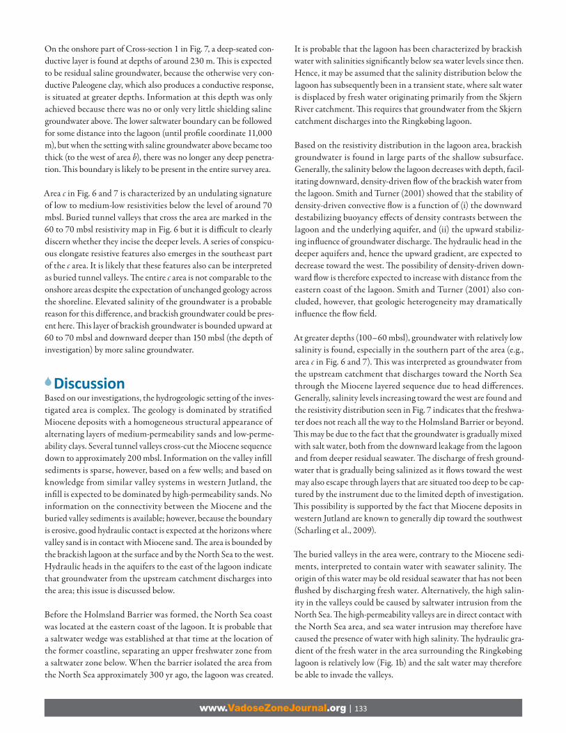
On the onshore part of Cross-section 1 in Fig. 7, a deep-seated con-

ductive layer is found at depths of around 230 m. Th is is expected

to be residual saline groundwater, because the otherwise very con-

ductive Paleogene clay, which also produces a conductive response,

is situated at greater depths. Information at this depth was only

achieved because there was no or only very little shielding saline

groundwater above. Th e lower saltwater boundary can be followed

for some distance into the lagoon (until profi le coordinate 11,000

m), but when the setting with saline groundwater above became too

thick (to the west of area b), there was no longer any deep penetra-

tion. Th is boundary is likely to be present in the entire survey area.

Area c in Fig. 6 and 7 is characterized by an undulating signature

of low to medium-low resistivities below the level of around 70

mbsl. Buried tunnel valleys that cross the area are marked in the

60 to 70 mbsl resistivity map in Fig. 6 but it is diffi cult to clearly

discern whether they incise the deeper levels. A series of conspicu-

ous elongate resistive features also emerges in the southeast part

of the c area. It is likely that these features also can be interpreted

as buried tunnel valleys. Th e entire c area is not comparable to the

onshore areas despite the expectation of unchanged geology across

the shoreline. Elevated salinity of the groundwater is a probable

reason for this diff erence, and brackish groundwater could be pres-

ent here. Th is layer of brackish groundwater is bounded upward at

60 to 70 mbsl and downward deeper than 150 mbsl (the depth of

investigation) by more saline groundwater.

DiscussionBased on our investigations, the hydrogeologic setting of the inves-

tigated area is complex. Th e geology is dominated by stratifi ed

Miocene deposits with a homogeneous structural appearance of

alternating layers of medium-permeability sands and low-perme-

ability clays. Several tunnel valleys cross-cut the Miocene sequence

down to approximately 200 mbsl. Information on the valley infi ll

sediments is sparse, however, based on a few wells; and based on

knowledge from similar valley systems in western Jutland, the

infi ll is expected to be dominated by high-permeability sands. No

information on the connectivity between the Miocene and the

buried valley sediments is available; however, because the boundary

is erosive, good hydraulic contact is expected at the horizons where

valley sand is in contact with Miocene sand. Th e area is bounded by

the brackish lagoon at the surface and by the North Sea to the west.

Hydraulic heads in the aquifers to the east of the lagoon indicate

that groundwater from the upstream catchment discharges into

the area; this issue is discussed below.

Before the Holmsland Barrier was formed, the North Sea coast

was located at the eastern coast of the lagoon. It is probable that

a saltwater wedge was established at that time at the location of

the former coastline, separating an upper freshwater zone from

a saltwater zone below. When the barrier isolated the area from

the North Sea approximately 300 yr ago, the lagoon was created.

It is probable that the lagoon has been characterized by brackish

water with salinities signifi cantly below sea water levels since then.

Hence, it may be assumed that the salinity distribution below the

lagoon has subsequently been in a transient state, where salt water

is displaced by fresh water originating primarily from the Skjern

River catchment. Th is requires that groundwater from the Skjern

catchment discharges into the Ringkøbing lagoon.

Based on the resistivity distribution in the lagoon area, brackish

groundwater is found in large parts of the shallow subsurface.

Generally, the salinity below the lagoon decreases with depth, facil-

itating downward, density-driven fl ow of the brackish water from

the lagoon. Smith and Turner (2001) showed that the stability of

density-driven convective fl ow is a function of (i) the downward

destabilizing buoyancy eff ects of density contrasts between the

lagoon and the underlying aquifer, and (ii) the upward stabiliz-

ing infl uence of groundwater discharge. Th e hydraulic head in the

deeper aquifers and, hence the upward gradient, are expected to

decrease toward the west. Th e possibility of density-driven down-

ward fl ow is therefore expected to increase with distance from the

eastern coast of the lagoon. Smith and Turner (2001) also con-

cluded, however, that geologic heterogeneity may dramatically

infl uence the fl ow fi eld.

At greater depths (100–60 mbsl), groundwater with relatively low

salinity is found, especially in the southern part of the area (e.g.,

area c in Fig. 6 and 7). Th is was interpreted as groundwater from

the upstream catchment that discharges toward the North Sea

through the Miocene layered sequence due to head diff erences.

Generally, salinity levels increasing toward the west are found and

the resistivity distribution seen in Fig. 7 indicates that the freshwa-

ter does not reach all the way to the Holmsland Barrier or beyond.

Th is may be due to the fact that the groundwater is gradually mixed

with salt water, both from the downward leakage from the lagoon

and from deeper residual seawater. Th e discharge of fresh ground-

water that is gradually being salinized as it fl ows toward the west

may also escape through layers that are situated too deep to be cap-

tured by the instrument due to the limited depth of investigation.

Th is possibility is supported by the fact that Miocene deposits in

western Jutland are known to generally dip toward the southwest

(Scharling et al., 2009).

Th e buried valleys in the area were, contrary to the Miocene sedi-

ments, interpreted to contain water with seawater salinity. Th e

origin of this water may be old residual seawater that has not been

fl ushed by discharging fresh water. Alternatively, the high salin-

ity in the valleys could be caused by saltwater intrusion from the

North Sea. Th e high-permeability valleys are in direct contact with

the North Sea area, and sea water intrusion may therefore have

caused the presence of water with high salinity. Th e hydraulic gra-

dient of the fresh water in the area surrounding the Ringkøbing

lagoon is relatively low (Fig. 1b) and the salt water may therefore

be able to invade the valleys.


Interpretation of the fl ow system in the area is complicated by the

historical changes in sea level and location of the coastline. During

the Litorina transgression approximately 7000 yr BP, the sea level

reached higher levels than presently with a coastline located to

the east of Ringkøbing fj ord. During the following regression

that resulted in present-day sea levels approximately 5000 yr BP,

displacement of salt water from especially the high-permeability

sediments is assumed to have taken place. Subsequently, the

Holmsland Barrier was generated about 300 yr ago, resulting in a

further withdrawal of the coastline to its present position. Hence,

the system is expected to be in a transient state where salt water

is displaced by fresh water. It is not possible, based on current

information, to give an unambiguous explanation of the current

distribution of salt water and fresh water in the area.

Th e knowledge obtained from this study suggests that SGD is

driven by both head gradients and convection, whereas drivers

such as the tide, waves, and currents are expected to be of minor

importance since the lagoon is protected by the Holmsland Barrier

and has a limited horizontal extent.

Apart from the geologic and hydrogeologic results, our studies

included an important technical result: SkyTEM data can pro-

duce accurate maps of bathymetry and salinity (Fig. 3) in areas of

shallow saline water, as long as the water depth is greater than a

few meters. To resolve such shallow layering at the very surface, we

used a regionally tuned starting model for the inversion over the

three distinct areas of the survey. It is important to note that we

did not include any constraints from prior information and that

the starting model did not include any regional variations, i.e., the

extracted information was actually resolved by the instrument and

cannot be considered an inversion artifact resulting from a perfect

starting model.

From the results in Fig. 3 and 6, it is evident that very small varia-

tions in resistivity can be resolved in the inversion, particularly

when the target resistivity is within the levels characteristic for

saline water. Th e ability to resolve such subtle diff erences suggests

that the method could potentially be used for resolving layering

within a water column, e.g., haloclines.

ConclusionsTh e presented models obtained from inversion of SkyTEM data

give a detailed description of the groundwater salinity distribu-

tion below the lagoon survey area. Based on these models, the area

is characterized by complicated and tightly coupled geologic and

hydrologic settings, combining into a spatially complex ground-

water salinity distribution including areas of fresh water, brackish

water, and seawater.

Buried tunnel valleys are found beneath the lagoon with a resistiv-

ity signature indicating saturation by seawater. Th e water fi lling

the buried valleys could be either residual seawater from before

the lagoon was formed or could come from a direct connection to

the North Sea.

A hypothesis of fl ow from the Skjern River catchment toward

the North Sea through both shallow and deeper lying aquifers is

supported by the geophysical results. Our results indicate outfl ow

from a shallow aquifer in the eastern part of the lagoon and also

reveal a deeper lying brackish aquifer for which the point of dis-

charge is more uncertain because it is located near the detection

limits of the instrument.

Additionally, it was demonstrated that accurate maps of both

bathymetry and seawater salinity can be produced from data

acquired with a calibrated SkyTEM instrument. Subtle diff erences

in resistivity were resolved by the inversion, suggesting that the

method could be used for mapping layered features within a water

column, such as haloclines.

AcknowledgmentsWe thank Anne-Sophie Christensen for seismic data processing and Jens Würgler Hansen, Environmental Centre of Ringkøbing, for supplying salinity data from the Ringkøbing lagoon. We also thank Bjarke Roth for assisting with the SkyTEM data processing, Grethe Storgaard for her help with making the fi gures, and Aaron Davis and Anders Vest Christiansen for proofreading. Th is study was funded by the Villum Foundation.

ReferencesAnthony, D., and I. Møller. 2002. The geological architecture and develop-

ment of the Holmsland Barrier and Ringkøbing Fjord area, Danish North Sea coast. Geogr. Tidsskr. 101:27–36.

Archie, G.E. 1942. The electrical resis vity log as an aid in determining some reservoir characteris cs. Trans. Am. Inst. Min. Metall. Pet. Eng. 146:54–62.

Auken, E., A.V. Chris ansen, B.H. Jacobsen, N. Foged, and K.I. Sørensen. 2005. Piecewise 1D laterally constrained inversion of resis vity data. Geophys. Prospect. 53:497–506.

Auken, E., A.V. Chris ansen, J.A. Westergaard, C. Kirkegaard, N. Foged, and A. Viezzoli. 2009a. An integrated processing scheme for high-resolu on airborne electromagne c surveys: The SkyTEM system. Explor. Geophys. 40:184–192.

Auken, E., A. Viezzoli, and A.V. Chris ansen. 2009b. A single so ware for pro-cessing, inversion, and presenta on of AEM data of diff erent systems. In Int. Geophys. Conf., 20th, Adelaide, SA, Australia [CD-ROM]. 22–25 Feb. 2009. Aust. Soc. Explor. Geophys., Perth, WA, Australia.

Burne , W.C., P.K. Aggarwal, A. Aureli, H. Bokuniewicz, J.E. Cable, M.A. Cha-re e, et al. 2006. Quan fying submarine groundwater discharge in the coastal zone via mul ple methods. Sci. Total Environ. 367:498–543.

Chris ansen, A.V., and E. Auken. 2008. Presen ng a free, highly fl exible inver-sion code. p. 1228–1232. In Expanded Abstr., Society of Explora on Geo-physics Annu. Meet., 78th, Las Vegas, NV. 9–14 Nov. 2008. SEG, Tulsa, OK.

Chris ansen, A.V., and E. Auken. 2010. A global measure for depth of inves- ga on in EM and DC modeling. In ASEG Ext. Abstr., Int. Geophys. Conf.,

21st, Sydney, NSW, Australia [CD-ROM]. 22–26 Aug. 2010. Aust. Soc. Ex-plor. Geophys., Perth, WA, Australia.

Christensen, N.B. 2000. Diffi cul es in determining electrical anisotropy in subsurface inves ga ons. Geophys. Prospect. 48:1–19.

d’Ozouville, N., E. Auken, K.I. Sørensen, S. Viole e, G. de Marsily, B. Deff on-taines, and G. Merlen. 2008. Extensive perched aquifer and structural implica ons revealed by 3D resis vity mapping in a Galapagos volcano. Earth Planet. Sci. Le . 269:518–522.

Fi erman, D.V., and M. Deszcz-Pan. 1998. Helicopter EM mapping of salt-water intrusion in Everglades Na onal Park, Florida. Explor. Geophys. 29:240–243.

Friborg, R., and S. Thomsen. 1999. Kortlægning af Ribe forma onen. Et fællesjysk grundvandssamarbejde. Tech. Rep. Ribe Amt, Ringkøbing Amt, Viborg Amt, Århus Amt, Vejle Amt, Sønderjyllands Amt.


Helsinki Commission. 2010. Manual for marine monitoring in the COMBINE Programme of HELCOM. Available at www.helcom.fi /groups/monas/CombineManual/en_GB/main (verifi ed 12 Nov. 2010). Helsinki Commis-sion, Helsinki, Finland.

Huuse, M., and H. Lykke-Andersen. 2000. Overdeepened Quaternary valleys in the eastern Danish North Sea: Morphology and origin. Quat. Sci. Rev. 19:1233–1253.

Jensen, K.H., and T.H. Illangasekare. 2011. HOBE: A hydrological observatory. Vadose Zone J. 10:1–7 (this issue).

Jørgensen, F., and P.B.E. Sandersen. 2006. Buried and open tunnel val-leys in Denmark: Erosion beneath mul ple ice sheets. Quat. Sci. Rev. 25:1339–1363.

Jørgensen, F., and P.B.E. Sandersen. 2009a. Buried valley mapping in Den-mark: Evalua ng mapping method constraints and the importance of data density. Z. Dtsch. Ges. Geowiss. 160:211–223.

Jørgensen, F., and P.B.E. Sandersen. 2009b. Kortlægning af begravede dale i Danmark, opdatering 2007–2009. Geol. Surv. of Denmark and Green-land, Copenhagen.

Jørgensen, F., P. Sandersen, E. Auken, H. Lykke-Andersen, and K.I. Sørensen. 2005. Contribu ons to the geological mapping of Mors, Denmark: A study based on a large-scale TEM survey. Bull. Geol. Soc. Den. 52:53–75.

Kafri, U., and M. Goldman. 2005. The use of the me domain electromag-ne c method to delineate saline groundwater in granular and carbonate aquifers and to evaluate their porosity. J. Appl. Geophys. 57:167–178.

Keller, G.V., and F.C. Frischknecht. 1966. Electrical methods in geophysical prospec ng. Pergamon Press, Oxford, UK.

Kirsch, R. 2006. Groundwater geophysics: A tool for hydrogeology. Springer-Verlag, Berlin.

Møller, I., H. Verner, V.H. Søndergaard, J. Flemming, E. Auken, and A.V. Chris- ansen. 2009. Integrated management and u liza on of hydrogeophysi-

cal data on a na onal scale. Near Surface Geophys. 7:647–659.Nielsen, L.H., and P. Japsen. 1991. Deep wells in Denmark 1935–1990:

Lithostratigraphic subdivision. Ser. A, Vol. 31. Geol Surv. Denmark, Copenhagen.

Nielsen, L., N.O. Jørgensen, and P. Gel ng. 2007. Mapping of the freshwater lens in a coastal aquifer on the Keta Barrier (Ghana) by transient electro-magne c soundings. J. Appl. Geophys. 62:1–15.

Nielsen, M.H., B. Rasmussen, and F. Gertz. 2005. A simple model for water level and stra fi ca on in Ringkøbing Fjord, a shallow, ar fi cial estuary. Estuarine Coastal Shelf Sci. 63:235–248.

Petersen, J.K., J.W. Hansen, M.B. Laursen, P. Clausen, J. Carstensen, and D.J. Conley. 2008. Regime shi in a coastal marine ecosystem. Ecol. Appl. 18:497–510.

Rasmussen, E.S. 2004. Stra graphy and deposi onal evolu on of the up-permost Oligocene–Miocene succession in western Denmark. Bull. Geol. Soc. Den. 51:89–109.

Ringkøbing Amt. 2004. Basisanalyse del I: Karakterisering af vandforekom-ster og opgørelse af påvirkninger.

Scharling, P.B., E.S. Rasmussen, T.O. Sonnenborg, P. Engesgaard, and K. Hinsby. 2009. Three-dimensional regional-scale hydrostra graphical modeling based on sequence stra graphical methods. Hydrogeol. J. 17:1913–1933.

Siemon, B., A.V. Chris ansen, and E. Auken. 2009. A review of helicopter-borne electromagne c methods for groundwater explora on. Near Surf. Geophys. 7:629–646.

Siemon, B., A. Steuer, U. Meyer, and H.-J. Rehli. 2007. HELP ACEH: A post-tsunami helicopter-borne groundwater project along the coasts of Aceh, northern Sumatra. Near Surf. Geophys. 5:231–240.

Smith, A.J., and J.V. Turner. 2001. Density-dependent surface water–ground-water interac on and nutrient discharge in the Swan–Canning estuary. Hydrol. Processes 15:2595–2616.

Sørensen, K.I., and E. Auken. 2004. SkyTEM: A new high-resolu on helicop-ter transient electromagne c system. Explor. Geophys. 35:191–199.

Sørensen, K.I., F. Eff ersø, and E. Auken. 2001. A hydrogeophysical inves ga- on of the Island of Drejø. Eur. J. Environ. Eng. Geophys. 6:109–124.

Sørensen, K.I., and F. Larsen. 1999. Ellog auger drilling: Three-in-one method for hydrogeological data collec on. Ground Water Monit. Rem. 19:97–101.

Viezzoli, A., A.V. Chris ansen, E. Auken, and K.I. Sørensen. 2008. Quasi-3D modeling of airborne TEM data by spa ally constrained inversion. Geo-physics 73:F105–F113.

Viezzoli, A., L. Tosi, P. Tea ni, and S. Silvestri. 2010. Surface water–ground-water exchange in transi onal coastal environments by airborne electro-magne cs: The Venice Lagoon example. Geophys. Res. Le . 37:L01402, doi:10.1029/2009GL041572.

Vrbancich, J. 2009. An inves ga on of seawater and sediment depth using a prototype airborne electromagne c instrument system: A case study in Broken Bay, Australia. Geophys. Prospect. 57:633–651.

Vrbancich, J. 2010. Preliminary inves ga ons using a helicopter me-do-main system for bathymetric measurements in shallow coastal waters? Port Lincoln and Broken Bay, NSW, Australia. In ASEG Ext. Abstr., Int. Geo-phys. Conf., 21st, Sydney, NSW, Australia [CD-ROM]. 22–26 Aug. 2010. Aust. Soc. Explor. Geophys., Perth, WA, Australia.

Vrbancich, J., and P.K. Fullagar. 2007. Improved seawater depth determina- on using corrected helicopter me-domain electromagne c data. Geo-

phys. Prospect. 55:407–420.

Salinity Distribution in Heterogeneous Coastal Aquifers Mapped by Airborne Electromagnetics

Documents

Transcript of Salinity Distribution in Heterogeneous Coastal Aquifers Mapped by Airborne Electromagnetics