CMTC 151042

Flow Simulation of CO2 Storage in Saline Aquifers Using a Black Oil Simulator Seyed Mohammad Shariatipour, SPE, G.E. Pickup, SPE, E.J. Mackay, SPE, Heriot-Watt University and N. Heinemann, University of Edinburgh

Copyright 2012, Carbon Management Technology Conference This paper was prepared for presentation at the Carbon Management Technology Conference held in Orlando, Florida, USA, 7–9 February 2012. This paper was selected for presentation by a CMTC program committee following review of information contained in an abstract submitted by the author(s). Contents of the paper have not been reviewed and are subject to correction by the author(s). The material does not necessarily reflect any position of the Carbon Management Technology Conference, its officers, or members. Electronic reproduction, distribution, or storage of any part of this paper without the written consent of the Carbon Management Technology Conference is prohibited. Permission to reproduce in print is restricted to an abstract of not more than 300 words; illustrations may not be copied. The abstract must contain conspi cuous acknowledgment of CMTC copyright..

Abstract Sequestration of carbon dioxide in geological formations has drawn increasing consideration as a potential method to reduce

the level of CO2 in the atmosphere, and therefore mitigate climate change. In particular, saline aquifers can potentially provide

a large storage volume world-wide. It is essential to assess the risk involved in storing CO2 in the subsurface, and simulations

of CO2 injection play an important role. Detailed simulations using a compositional simulator, which solves the equation of

state for the fluids and calculates the partitioning of fluids between phases, is time consuming. It is therefore advantageous to

use a simpler method for simulation, such as a modification of a black-oil simulator (designed for use in the oil industry),

where fluid properties are input using look-up tables.

In this study, we have tested the accuracy of flow simulations of CO2 storage in saline aquifers using a black-oil simulator

(BOS) compared with a compositional simulator (CS). A range of models was investigated: 2D, 3D and radial models,

horizontal and tilted, and homogeneous and heterogeneous. On the whole the results compared well, although accuracy of the

BOS depended on the type of grid used, being less accurate for radial models, where discretisation effects were evident.

In agreement with other studies, we found that the black-oil simulations were, on average, a factor of four faster than

compositional simulations.

Introduction CO2 capture and storage has attracted much attention in recent years as a method to reduce the greenhouse gas emissions to the

atmosphere and thus meeting the requirements of the Kyoto protocol (December, 1997). Mechanisms to trap large amounts of

CO2 include dissolution into the oceans, sorption by vegetation and geological sequestration. Several geological settings are

envisaged as potentials storage sites which can be accomplished by the aid of oil and gas reservoirs, either reservoirs in

production giving enhanced oil recovery, or abandoned reservoirs, non mineable coal seems, and deep saline aquifers. It

should be noted that in all cases the CO2 should be stored as a supercritical fluid. The critical point of CO2 is 31.1°C and 73.9

bars, above which CO2 has a high density, like a liquid, but it still acts as a gas (IPCC, 2005). This is achieved by storing the

CO2 at a depth of more than 800 meters. This study focused on CO2 storage in saline aquifers. It is important to be aware of

the factors affecting CO2 migration in the saline aquifers, such as advection, buoyancy and thermal effects and the influence of

reservoir heterogeneity (e.g. Ukaegbu et al, 2009). CO2 is retained in situ through four basic trapping mechanisms:

stratigraphic and structural, solubility, residual trapping at the pore scale and mineral trapping.

Compositional simulation was originally developed for modeling enhanced oil recovery processes, such as miscible gas

injection. More recently, compositional simulation packages have been extended to model CO2 injection into saline aquifers,

including the mutual solubility of CO2 and brine and the increase of the density of brine with dissolved CO2 (e.g. CO2STORE

module, Schlumberger, 2010). However, assuming the CO2 is pure and is always in a supercritical state, the simulation of CO2

storage is a simpler procedure than miscible gas injection. In this case, fully compositional simulation is unnecessary, and the

PVT properties can be input using pre-calculated tables. One method of doing this is to adapt black-oil simulators for CO2

storage. In this case, oil is used to represent brine and hydrocarbon gas represents supercritical CO2.

Spycher et al. (2003) developed a method for calculating the phase equilibrium and the mutual solubilities of CO2 from 12

to 110 °C and pure H2O from 15 to 100 °C and up to 600 bar. They used the modified Redlich-Kwong equation of state to

2 CMTC 151042

express departure from ideal behavior. They concluded that the solubility of CO2 rises dramatically with increasing pressure

up to saturation pressure, but decreases with rising temperature. In this work there is, on the whole, a good match between

experimental and calculated solubilities from 12 up to 50 °C and up to pressure 600 bars, which is important for geological

sequestration purposes.

Spycher and Pruess (2005) describe a continuation of the work of the previous study on mutual solubilities of CO2 and

H2O (Spycher et al, 2003) to include the partitioning in chloride brines, at the same pressures and temperatures as the previous

study. They presented an extended formulation which accounted for the effect of dissolved salts for solutions up to 6 molal

NaCl and 4 molal CaCl2. The water mole fraction in the CO2 rich phase (2

H Oy ) and the CO2 mole fractions in the aqueous

phase (2

COx ) are respectively expressed as:

2

2 2

2

2

0

0

1exp

55.508

COCO H O tot

CO

x CO g

y P P P Vx

K RT

(1)

22 2

2

2

0 0

expH OH O H O

H O

H O tot

K a P P Vy

P RT

(2)

where P is pressure, K is the equilibrium ratio, V is average molar volume, is the fugacity coefficient, T is temperature, R is

the gas constant and x is the ratio of the mole fraction of CO2 dissolved in pure water divided by the mole fraction dissolved

in brine. The subscript tot stands for total and superscript 0 for a reference value.

Hassanzadeh et al. (2008) developed an efficient algorithm to convert compositional data from an equation of state to black

oil PVT data. Their algorithm is capable of generating CO2-brine density, solubility and formation volume factor which are

necessary for use in black-oil flow simulations of CO2 storage in geological formations. Hassanzadeh et al. (2008) used those

equations which were presented by Spycher et al. (2003) and Spycher and Pruess (2005) to generate their algorithm and finally

to generate PVT data for a black-oil model. In their calculation, they used constant mole fraction for salt as they believe that

CO2 solubility in aqueous phase is fairly low for the pressure and temperature range of CO2 storage in the saline aquifers. The

final equations which they used for the calculation of dissolved gas-brine ratio, Rs, and the brine formation volume factor, Bb,

are as follows:

2

2 2

,

,1

b SC CO

s

CO SC CO

xR

x

, (3)

where ,b SC

and 2

,CO SC are the formation brine and CO2 molar density at standard conditions, and

2CO

x is the CO2 mole

fraction in aqueous phase.

,

, 21

b SC

b

b res

Bco

, (4)

Where ,b SC

and ,b res

are the formation brine mass density at standard and at reservoir conditions, respectively. 2

co is the

CO2 mass fraction in the aqueous phase.

Hassanzadeh et al (2008) used the Computer Modeling Group software to investigate the run times for the simulation of

CO2 storage in a saline aquifer using both a black oil simulator (IMEX, 2004) and a compositional one (GEM, 2004). The

results showed that the black oil simulator performed three to four times faster than the compositional model.

Methodology

Model Specification

In this study, CO2 was injected into 2D homogeneous and heterogeneous models, both horizontal and tilted. The results of

these simulations were evaluated by comparing the average pressure (FPR), the average gas saturation value (FGSAT), the

well bottom hole pressure (WBHP) and gas in place in the gas phase (GIPG). Then 3D homogeneous and heterogeneous

models, and a radial model were also tested (Table 1). As can be seen from Table 1, similar properties were used for all the

models, so that the focus was on the PVT properties of the fluids in the black-oil and compositional simulations. In addition,

all the models had the same volume, so that the pressure increase was the same.

CMTC 151042 3

There are two phases present in this model: CO2 represents the gaseous phase and the formation water (brine) is treated as

oil, so we used brine and CO2 PVT data instead of oil and gas in black oil simulator. In all cases, a single CO2 injection well

was placed in the centre of each model. The simulations ran over a period of 120 years altogether, with CO2 injection taking

place during the first 20 years, followed by a period of shut-in lasting 100 years. The injection was controlled by rate. In all

the models cases the injection rate was the same.

Table 1 Models used in this study Two Dimensions Three Dimensions Radial Grid

Model Properties Homogeneous Heterogeneous Homogeneous Heterogeneous Homogeneous

Total size, m 2000*100*100 2000*100*100 2000*100*100 2000*100*100 252*252*100

No. of cells 81*1*81 81*1*81 81*20*40 81*20*40 81*2*81

Porosity, Fraction 0.2 0.05 - 0.2 0.2 0.05 - 0.2 0.2

Permeability, mD 100 1 - 100 100 1 - 100 100

The following additional assumptions were made:

The processes during injection and after shut-in were isothermal (35°C).

The mineral trapping mechanism was ignored.

Solid precipitation is negligible.

CO2 is injected as supercritical fluid phase; no impurities were present.

The models initially contained 100% brine. The initial model properties were based on Birkholzer et al. (2008), who described the large-scale impact of CO2 storage in

deep saline aquifers. Figure 1 illustrates the initial conditions which Birkholzer et al. (2008) used for their model, and indicates

the values used in this study.

Figure 1 initial conditions, Birkholzer et al. (2008).

The simulators which were used for this study were the black oil simulator, Eclipse 100 (Schlumberger, 2010) and the

compositional simulator, Eclipse 300 with the CO2STORE module (Schlumberger, 2010). The PVT data used in this project

were generated using the ECO2N module of the TOUGH2 software package (Pruess, 2005). In the results below, we refer to

black-oil simulation as "BOS" and compositional simulation as "CS". There are differences in the way in which fluid

properties are calculated in the ECO2N and the Eclipse 300 software packages. For example, the Eclipse 300 CO2STORE

module uses the method of Pruess and Spycher (2005) to calculate the mole fraction of CO2 dissolved in brine. However, the

EOC2N software uses a modification of the method (Pruess 2005). Also, these package use different formulae for calculating

the densities and viscosities of the fluids.

Results

2D Models

2D Homogeneous Models

Average pressure

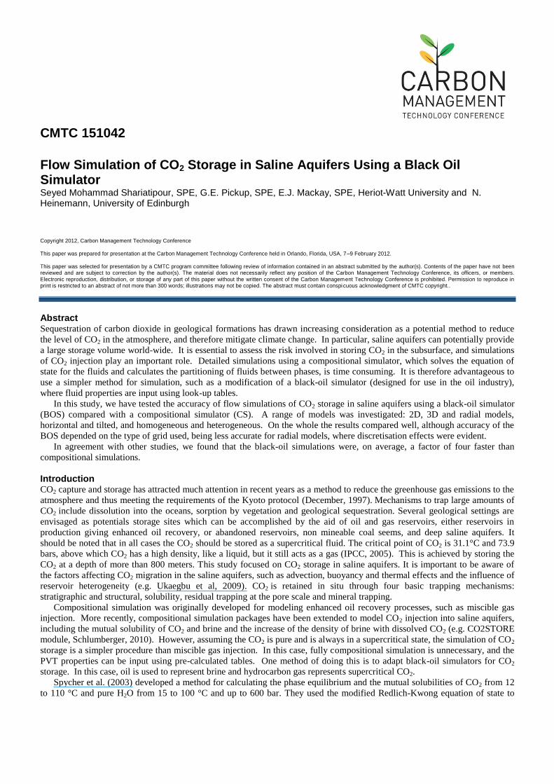
Figure 2 shows the average model pressure values (FPR) for the horizontal and tilted 2D homogeneous models. The

results show reasonable agreement. The pressure rises dramatically as CO2 is injected into the aquifer from 2010 to 2030, and

4 CMTC 151042

then subsequently decreases slowly, as CO2 dissolves. In the post injection period, the pressure in the black oil simulations

decreases at a slightly slower rate than the in the compositional simulations, indicating that there is less dissolution in the black

oil simulations. The difference in pressure is 1.5 bars in the horizontal case and 1.4 bars in the tilted case.

Gas saturation average value

Figure 3 reveals that both simulators (black oil and compositional) provided close results for the average gas saturation.

The results for the homogeneous models show that the use of Eclipse 100 with the PVT properties calculated using TOUGH2

and ECO2N are compatible with Eclipse 300.

Figure 2 Average pressure values for 2D homogeneous models in BOS and CS models

Figure 3 Gas saturation average values for 2D homogeneous models

2D Heterogeneous Models

Average pressure

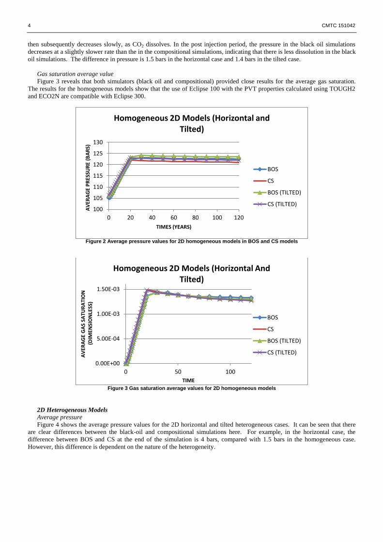
Figure 4 shows the average pressure values for the 2D horizontal and tilted heterogeneous cases. It can be seen that there

are clear differences between the black-oil and compositional simulations here. For example, in the horizontal case, the

difference between BOS and CS at the end of the simulation is 4 bars, compared with 1.5 bars in the homogeneous case.

However, this difference is dependent on the nature of the heterogeneity.

100

105

110

115

120

125

130

0 20 40 60 80 100 120

AV

ERA

GE

PR

ESSU

RE

(BA

RS)

TIMES (YEARS)

Homogeneous 2D Models (Horizontal and Tilted)

BOS

CS

BOS (TILTED)

CS (TILTED)

0.00E+00

5.00E-04

1.00E-03

1.50E-03

0 50 100

AV

ERA

GE

GA

S SA

TUR

ATI

ON

(

DIM

ENSI

ON

LESS

)

TIME

Homogeneous 2D Models (Horizontal And Tilted)

BOS

CS

BOS (TILTED)

CS (TILTED)

CMTC 151042 5

Gas saturation

Figure 5 demonstrates that both simulators (black oil and compositional) provided close results for gas saturation

distribution.

Figure 4 Average Pressure values For 2D Heterogeneous Models.

Figure 5 Gas Saturation For 2D Heterogeneous Models.

3D Models

3D Homogeneous Models

Average pressure

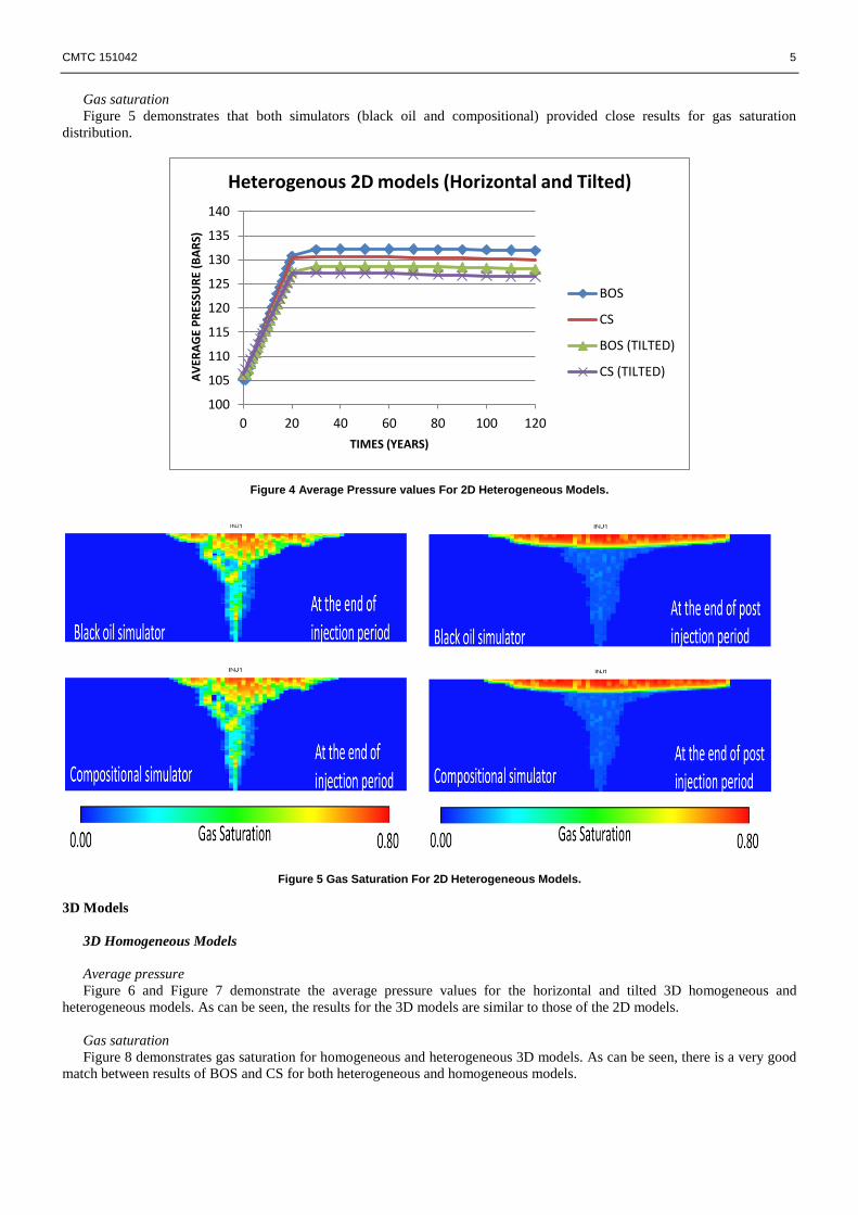
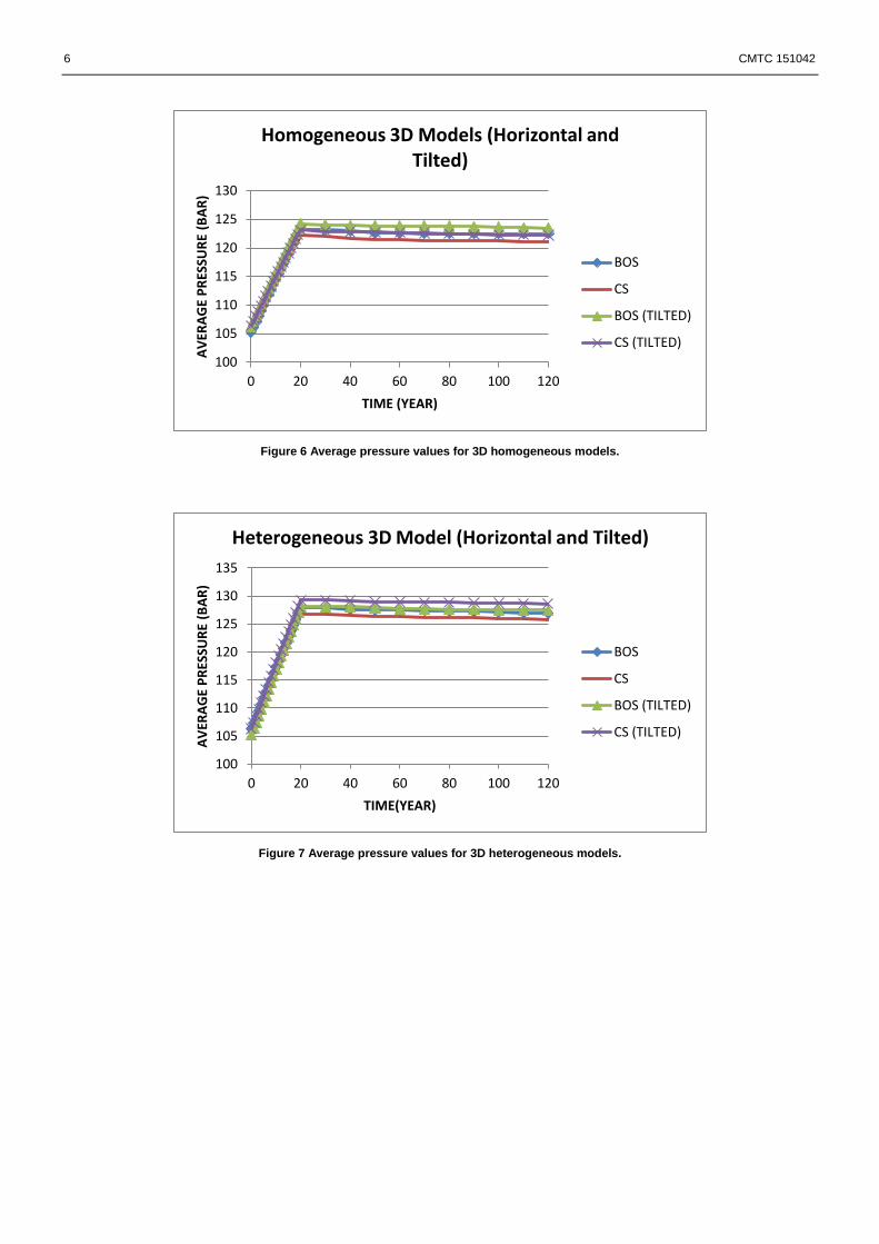
Figure 6 and Figure 7 demonstrate the average pressure values for the horizontal and tilted 3D homogeneous and

heterogeneous models. As can be seen, the results for the 3D models are similar to those of the 2D models.

Gas saturation

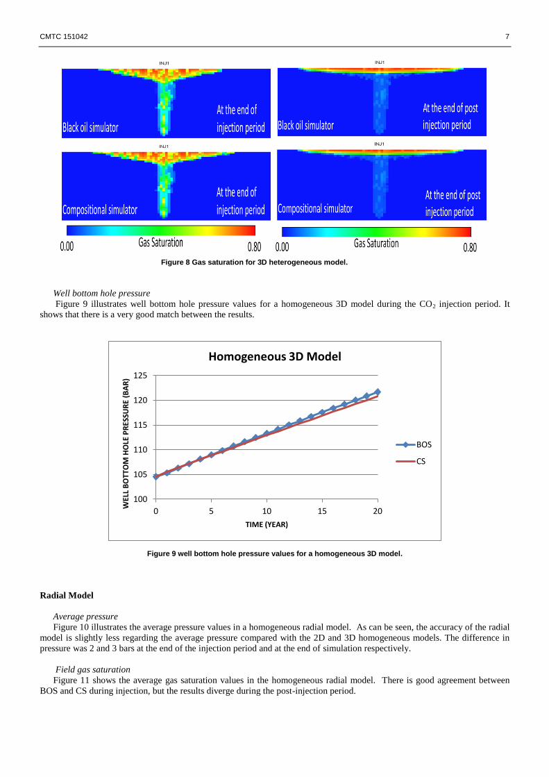
Figure 8 demonstrates gas saturation for homogeneous and heterogeneous 3D models. As can be seen, there is a very good

match between results of BOS and CS for both heterogeneous and homogeneous models.

100

105

110

115

120

125

130

135

140

0 20 40 60 80 100 120

AV

ERA

GE

PR

ESSU

RE

(BA

RS)

TIMES (YEARS)

Heterogenous 2D models (Horizontal and Tilted)

BOS

CS

BOS (TILTED)

CS (TILTED)

6 CMTC 151042

Figure 6 Average pressure values for 3D homogeneous models.

Figure 7 Average pressure values for 3D heterogeneous models.

100

105

110

115

120

125

130

0 20 40 60 80 100 120

AV

ERA

GE

PR

ESSU

RE

(BA

R)

TIME (YEAR)

Homogeneous 3D Models (Horizontal and Tilted)

BOS

CS

BOS (TILTED)

CS (TILTED)

100

105

110

115

120

125

130

135

0 20 40 60 80 100 120

AV

ERA

GE

PR

ESSU

RE

(BA

R)

TIME(YEAR)

Heterogeneous 3D Model (Horizontal and Tilted)

BOS

CS

BOS (TILTED)

CS (TILTED)

CMTC 151042 7

Figure 8 Gas saturation for 3D heterogeneous model.

Well bottom hole pressure

Figure 9 illustrates well bottom hole pressure values for a homogeneous 3D model during the CO2 injection period. It

shows that there is a very good match between the results.

Figure 9 well bottom hole pressure values for a homogeneous 3D model.

Radial Model

Average pressure

Figure 10 illustrates the average pressure values in a homogeneous radial model. As can be seen, the accuracy of the radial

model is slightly less regarding the average pressure compared with the 2D and 3D homogeneous models. The difference in

pressure was 2 and 3 bars at the end of the injection period and at the end of simulation respectively.

Field gas saturation

Figure 11 shows the average gas saturation values in the homogeneous radial model. There is good agreement between

BOS and CS during injection, but the results diverge during the post-injection period.

100

105

110

115

120

125

0 5 10 15 20

WEL

L B

OTT

OM

HO

LE P

RES

SUR

E (B

AR

)

TIME (YEAR)

Homogeneous 3D Model

BOS

CS

8 CMTC 151042

Well bottom hole pressure

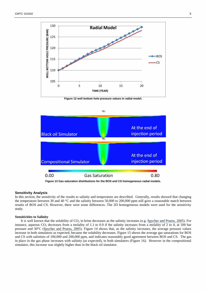
As can be seen from Figure 12 the well bottom hole pressure values in the BOS are slightly greater than the CS values. The

absolute difference in pressure reached 2.5 bars at the end of the CO2 injection period.

The above results show that the BOS results for the radial model were less accurate than for the rectangular models. Further

investigation of the radial simulation results showed that the gas saturation distributions were very similar, the only difference

being slightly higher saturation levels in the BOS model (hence the higher pressures). Figure 13 illustrates the saturation

distribution for the BOS and CS radial models at the end of the injection period and demonstrates that BOS adequately

simulates the migration of the plume.

Radial models are useful for simulating injection due to the high grid resolution around the well. However, these small

grid cells are a disadvantage in the post-injection period. In the case considered here, small differences in the solubility of CO2

in the two simulations led to a significant difference in the average saturation.

Figure 10 Average pressure values in a homogeneous radial model.

Figure 11 Gas saturation average values in a homogeneous radial model.

100

105

110

115

120

125

130

0 20 40 60 80 100 120

AV

ERA

GE

PR

ESSU

RE

(BA

R)

TIME (YEAR)

Radial Model

BOS

CS

0

0.0002

0.0004

0.0006

0.0008

0.001

0.0012

0.0014

0.0016

0.0018

0 20 40 60 80 100 120

GA

S SA

TUR

ATI

ON

AV

ERA

GE

(DIM

ENSI

ON

LESS

)

TIME (YEAR)

Radial Model

BOS

CS

CMTC 151042 9

Figure 12 well bottom hole pressure values in radial model.

Figure 13 Gas saturation distributions for the BOS and CS homogeneous radial models.

Sensitivity Analysis In this section, the sensitivity of the results to salinity and temperature are described. Generally, results showed that changing

the temperature between 30 and 40 °C and the salinity between 50,000 to 200,000 ppm still gave a reasonable match between

results of BOS and CS. However, there were some differences. The 2D homogeneous models were used for the sensitivity

study.

Sensitivities to Salinity

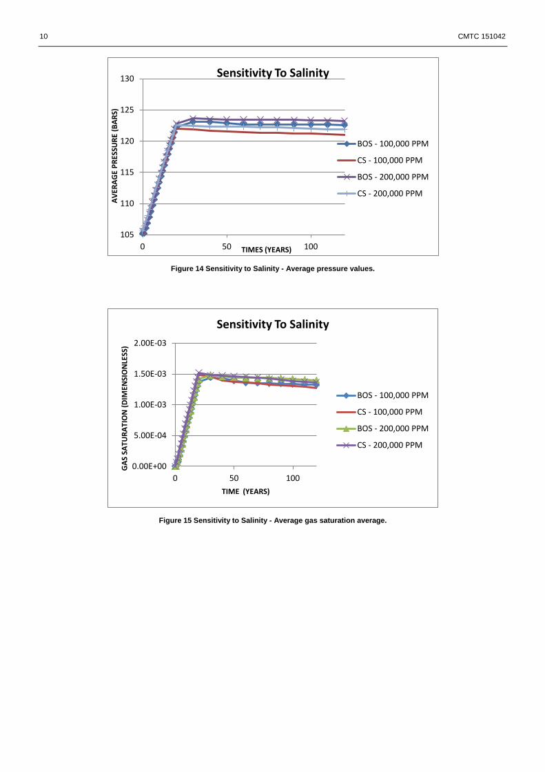
It is well known that the solubility of CO2 in brine decreases as the salinity increases (e.g. Spycher and Pruess, 2005). For

instance, aqueous CO2 decreases from a molality of 1.1 to 0.9 if the salinity increases from a molality of 2 to 4, at 100 bar

pressure and 30°C (Spycher and Pruess, 2005). Figure 14 shows that, as the salinity increases, the average pressure values

increase in both simulators as expected, because the solubility decreases. Figure 15 shows the average gas saturations for BOS

and CS with salinities of 100,000 and 200,000 ppm, and indicates reasonably good agreement between BOS and CS. The gas

in place in the gas phase increases with salinity (as expected), in both simulators (Figure 16). However in the compositional

simulator, this increase was slightly higher than in the black oil simulator.

105

110

115

120

125

130

0 5 10 15 20

WEL

L B

OTT

OM

HO

LE P

RES

SUR

E (B

AR

)

TIME (YEAR)

Radial Model

BOS

CS

10 CMTC 151042

Figure 14 Sensitivity to Salinity - Average pressure values.

Figure 15 Sensitivity to Salinity - Average gas saturation average.

105

110

115

120

125

130

0 50 100

AV

ERA

GE

PR

ESSU

RE

(BA

RS)

TIMES (YEARS)

Sensitivity To Salinity

BOS - 100,000 PPM

CS - 100,000 PPM

BOS - 200,000 PPM

CS - 200,000 PPM

0.00E+00

5.00E-04

1.00E-03

1.50E-03

2.00E-03

0 50 100

GA

S SA

TUR

ATI

ON

(D

IMEN

SIO

NLE

SS)

TIME (YEARS)

Sensitivity To Salinity

BOS - 100,000 PPM

CS - 100,000 PPM

BOS - 200,000 PPM

CS - 200,000 PPM

CMTC 151042 11

Figure 16 Sensitivity to Salinity - Gas in place in gas phase

Sensitivity to temperature

As the temperature increases, the solubility of CO2 in brine decreases. For instance: an increase in temperature from 30 oC

to 60 oC at 100 bar for a solvent with 1 molal NaCl, causes the solubility of CO2 to decrease from a molality of 1.1 to 0.85

(Spycher and Pruess, 2005).

The average pressure increased as the temperature increased from 30 to 40 oC, as expected (Figure 17). For both

temperatures, the pressure was 2 bars higher in the BOS case than in the CS case. Figure 18 demonstrates that the gas

saturation increases as the temperature increases, due to the lower dissolution. The well bottom hole pressure values increase

with increasing temperature as expected (Figure 19).

Figure 17 Sensitivity to temperature - Average pressure values

0

1

2

3

4

5

6

BOS CS

GA

S IN

PLA

CE

IN G

AS

PH

ASE

(SM

3)

x 1

00

00

00

0 Sensitivity To Salinity

Sum Of Absolute Value Of Diffference Between Model With 200000 PPM And 100000 PPM Salinity

105

110

115

120

125

130

135

140

0 20 40 60 80 100 120

AV

ERA

GE

PR

ESSU

RE

(BA

RS)

TIMES (YEARS)

Sensitivity To Temperature

BOS - 40 C

CS - 40 C

BOS - 30 C

12 CMTC 151042

Figure 18 Sensitivity to temperature - Gas saturation average value.

Figure 19 Sensitivity to temperature - Well bottom hole pressure values.

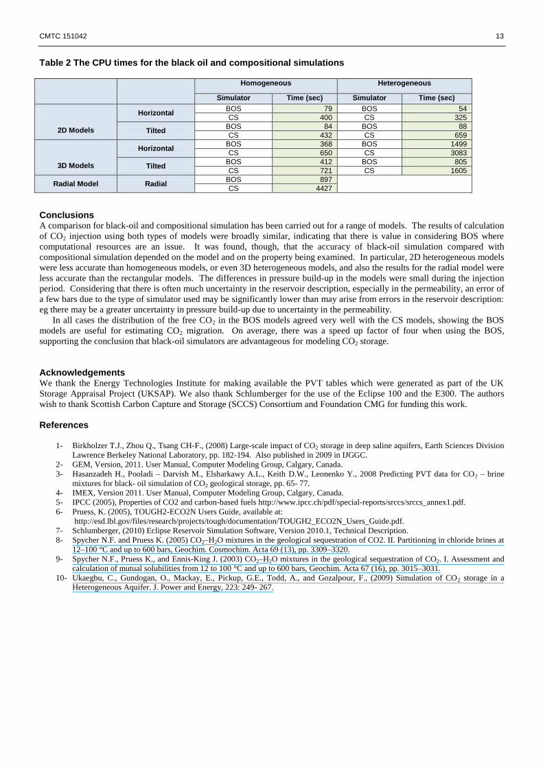
Simulations Run Times Table 2 illustrates the CPU times for the different models using both simulators. The minimum and maximum time steps were

set to the same values in both types of simulation. In the simulation study performed here, it was found that the CPU times

depend on the number of cells in each model and the heterogeneity of the models. The speed up factor when using the BOS

ranged from approximately 2 (for the 3D models - homogeneous and heterogeneous) to 7.5 (2D tilted heterogeneous model),

with an average speed up factor of 4.

0.00E+00

5.00E-04

1.00E-03

1.50E-03

2.00E-03

2.50E-03

0 20 40 60 80 100 120

GA

S SA

TUR

ATI

ON

(D

IMEN

SIO

NLE

SS)

TIME (YEARS)

Sensitivity To Temperature

BOS - 40 C

CS - 40 C

CS - 30 C

BOS - 30 C

100

105

110

115

120

125

130

135

140

0 5 10 15 20 WEL

L B

OTT

OM

HO

LE P

RES

SUR

E (B

AR

S)

TIME (YEARS)

Sensitivity To Temperature

BOS - 4O C

CS - 40 C

BOS - 30 C

CS - 30 C

CMTC 151042 13

Table 2 The CPU times for the black oil and compositional simulations Homogeneous Heterogeneous

Simulator Time (sec) Simulator Time (sec)

2D Models

Horizontal BOS 79 BOS 54

CS 400 CS 325

Tilted BOS 84 BOS 88

CS 432 CS 659

3D Models

Horizontal BOS 368 BOS 1499

CS 650 CS 3083

Tilted BOS 412 BOS 805

CS 721 CS 1605

Radial Model Radial BOS 897

CS 4427

Conclusions A comparison for black-oil and compositional simulation has been carried out for a range of models. The results of calculation

of CO2 injection using both types of models were broadly similar, indicating that there is value in considering BOS where

computational resources are an issue. It was found, though, that the accuracy of black-oil simulation compared with

compositional simulation depended on the model and on the property being examined. In particular, 2D heterogeneous models

were less accurate than homogeneous models, or even 3D heterogeneous models, and also the results for the radial model were

less accurate than the rectangular models. The differences in pressure build-up in the models were small during the injection

period. Considering that there is often much uncertainty in the reservoir description, especially in the permeability, an error of

a few bars due to the type of simulator used may be significantly lower than may arise from errors in the reservoir description:

eg there may be a greater uncertainty in pressure build-up due to uncertainty in the permeability.

In all cases the distribution of the free CO2 in the BOS models agreed very well with the CS models, showing the BOS

models are useful for estimating CO2 migration. On average, there was a speed up factor of four when using the BOS,

supporting the conclusion that black-oil simulators are advantageous for modeling CO2 storage.

Acknowledgements We thank the Energy Technologies Institute for making available the PVT tables which were generated as part of the UK

Storage Appraisal Project (UKSAP). We also thank Schlumberger for the use of the Eclipse 100 and the E300. The authors

wish to thank Scottish Carbon Capture and Storage (SCCS) Consortium and Foundation CMG for funding this work. References

1- Birkholzer T.J., Zhou Q., Tsang CH-F., (2008) Large-scale impact of CO2 storage in deep saline aquifers, Earth Sciences Division

Lawrence Berkeley National Laboratory, pp. 182-194. Also published in 2009 in IJGGC.

2- GEM, Version, 2011. User Manual, Computer Modeling Group, Calgary, Canada.

3- Hasanzadeh H., Pooladi – Darvish M., Elsharkawy A.L., Keith D.W., Leonenko Y., 2008 Predicting PVT data for CO2 – brine

mixtures for black- oil simulation of CO2 geological storage, pp. 65- 77.

4- IMEX, Version 2011. User Manual, Computer Modeling Group, Calgary, Canada.

5- IPCC (2005), Properties of CO2 and carbon-based fuels http://www.ipcc.ch/pdf/special-reports/srccs/srccs_annex1.pdf.

6- Pruess, K. (2005), TOUGH2-ECO2N Users Guide, available at:

http://esd.lbl.gov/files/research/projects/tough/documentation/TOUGH2_ECO2N_Users_Guide.pdf.

7- Schlumberger, (2010) Eclipse Reservoir Simulation Software, Version 2010.1, Technical Description.

8- Spycher N.F. and Pruess K. (2005) CO2–H2O mixtures in the geological sequestration of CO2. II. Partitioning in chloride brines at

12–100 °C and up to 600 bars, Geochim. Cosmochim. Acta 69 (13), pp. 3309–3320.

9- Spycher N.F., Pruess K., and Ennis-King J. (2003) CO2–H2O mixtures in the geological sequestration of CO2. I. Assessment and

calculation of mutual solubilities from 12 to 100 °C and up to 600 bars, Geochim. Acta 67 (16), pp. 3015–3031.

10- Ukaegbu, C., Gundogan, O., Mackay, E., Pickup, G.E., Todd, A., and Gozalpour, F., (2009) Simulation of CO2 storage in a

Heterogeneous Aquifer. J. Power and Energy, 223: 249- 267.