Texas Water Development Board

Report 365

Aquifers of the Gulf Coast of Texas

edited by Robert E. Mace, Sarah C. Davidson, Edward S. Angle, and William F. Mullican, III February 2006

ii

This page intentionally blank.

iii

Texas Water Development Board

E. G. Rod Pittman, Chairman, Lufkin Thomas Weir Labatt, III, Member, San Antonio

Jack Hunt, Vice Chairman, Houston James E. Herring, Member, Amarillo

Dario Vidal Guerra, Jr., Member, Edinburg William W. Meadows, Member, Fort Worth

J. Kevin Ward, Executive Administrator

Authorization for use or reproduction of any original material contained in this publication, i.e., not obtained from other sources, is freely granted. The Board would appreciate acknowledgment. The use of brand names in this publication does not indicate an endorsement by the Texas Water Development Board or the State of Texas.

With the exception of papers written by Texas Water Development Board staff, views expressed in this report are of the authors and do not necessarily reflect the views of the Texas Water Development Board.

Published and distributed by the

Texas Water Development Board P.O. Box 13231, Capitol Station

Austin, Texas 78711-3231

February 2006 Report 365

(Printed on recycled paper)

iv

This page intentionally blank.

v

Note from the Editors: The Gulf Coast is prominent in the history of Texas. The first sight of Texas by western explorers was our Gulf Coast. Texans defeated Santa Anna to earn their independence from Mexico amid the swamps at San Jacinto. And the oil that erupted from Spindletop, south of Beaumont, propelled Texas into the oil and gas industry. Groundwater from the Gulf Coast area has also played an important, although perhaps quieter, part of Texas’ history as well. As Texas and its communities grew, Texans looked below the land surface for water and found a plentiful source in the Gulf Coast aquifer as well as other aquifers. With a fickle climate, farmers tapped into the aquifer to supplement rainfall and grow more profitable crops. Industries relied on the aquifer to support their manufacturing. The Gulf Coast aquifer will likely be quietly prominent in the future as well, as Texas continues to grow. Inland cities, regional water planning groups, and river authorities are considering conjunctive use projects—the coordinated use of different sources of water to optimize water use and minimize the adverse effects that can come from relying on a single source—that include the Gulf Coast aquifer. With improvements in desalination technologies, even poor quality water from the aquifer in the Lower Rio Grande Valley and close to the coast is proving to be a valuable resource. Water continues to fuel the growth and prosperity of Texas.

Our hope is that this report will be useful to those attempting to better understand and manage the aquifers of the Gulf Coast region of Texas. This report, the third in a series of reports that will summarize the groundwater resources of Texas, represents the proceedings of a conference held on February 16, 2006, at the Texas A&M University—Corpus Christi campus. Similar to the previous two reports in the “Aquifers of Texas” series, we identified topics we wanted addressed and then identified potential contributors to write chapters and give a presentation at the conference. This document is meant to be a stand alone document—a book about the Gulf Coast aquifer in Texas—as well as a proceedings of the conference held in Corpus Christi.

This conference and this report are the result of the hard work and cooperation of many people, and we are thankful for everyone’s patience, assistance, and generosity. First, we thank our speakers and authors for their contributions to the conference and their willingness to share their knowledge. We also thank Rick Hay, Jennifer Smith-Engle, and the staff at the Harte Research Institute—all at Texas A&M University–Corpus Christi—for providing space for the conference and assistance in running the conference. We are grateful to many at the Texas Water Development Board for their assistance and support, including Mike Parcher for his assistance in preparing and printing the report and Dr. Ali Chowdhury for providing us needed papers and topics on short notice. Finally, we thank our Board and our Executive Administrator, J. Kevin Ward, for their continued support of these conferences to inform Texans about their groundwater.

Robert E. Mace Sarah Davidson Edward S. Angle William F. Mullican, III

vi

Table of Contents

Note from the Editors...................................................................................................... v

1. Aquifers of the Gulf Coast of Texas: An Overview by Sarah C. Davidson and Robert E. Mace .................................................................... 1

2. Geology of the Gulf Coast Aquifer, Texas by Ali H. Chowdhury and Mike J. Turco ...................................................................... 23

3. The Yegua-Jackson Aquifer by Richard D. Preston................................................................................................... 51

4. Conjunctive Use of the Brazos River Alluvium Aquifer by David O’Rourke ....................................................................................................... 61

5. Hydrogeochemistry, Salinity Distribution, and Trace Constituents: Implications for Salinity Sources, Geochemical Evolution, and Flow Systems Characterization, Gulf Coast Aquifer, Texas by Ali H. Chowdhury, Radu Boghici, and Janie Hopkins ............................................. 81

6. Stratigraphy, Lithology, and Hydraulic Properties of the Chicot and Evangeline Aquifers in the LSWP Study Area, Central Texas Coast by Steven C. Young, Paul R. Knox, Van Kelley, Trevor Budge, Neil Deeds, William E. Galloway, and Ernest T. Baker ................................................................. 129

7. 100 Years of Groundwater Use and Subsidence in the Upper Texas Gulf Coast by Thomas A. Michel................................................................................................... 139

8. Dry Periods and Drought Events of the Gulf Coastal Region by Robert G. Bradley .................................................................................................. 149

9. The Impact of Groundwater Flows on Estuaries by John A. Breier ........................................................................................................ 165

10. Groundwater Models of the Gulf Coast Aquifer of Texas by Ali H. Chowdhury and Robert E. Mace ................................................................. 173

11. Optimization-Based Approaches for Groundwater Management by Venkatesh Uddameri, Muthukumar Kuchanur, and Naresh Balija ....................... 205

12. Salt Domes in the Gulf Coast Aquifer by H. Scott Hamlin ...................................................................................................... 217

13. Status Report on Brackish Groundwater and Desalination in the Gulf Coast Aquifer of Texas by Sanjeev Kalaswad and Jorge Arroyo ..................................................................... 231

vii

14. Brackish Water Desalination in South Texas: An Alternative to the Rio Grande by Joseph W. (Bill) Norris .......................................................................................... 241

15. Effects of Oil and Gas Production on Groundwater by John James Tintera and Leslie Savage .................................................................. 255

16. History of Production and Potential Future Production of the Gulf Coast Aquifer by W. John Siefert, Jr. and Chris Drabek ................................................................... 261

17. The Challenge of Managing Groundwater in the Gulf Coast Aquifer: Recognizing and Incorporating Divergent Value Systems Regarding Groundwater as a Resource by James A. Dodson .................................................................................................... 273

18. Assessment of Shallow Recharge and Groundwater-Surface Water Interactions for the LSWP Study Region, Central Texas Coast by Niel Deeds, Van Kelley, Steven C. Young, and Geoffrey P. Saunders ................... 287

19. Low Flow Gain-Loss Study of the Colorado River in Texas by Geoffrey P. Saunders ............................................................................................. 293

20. Groundwater Management through Groundwater Conservation Districts by the Texas Alliance of Groundwater Districts ......................................................... 299

viii

This page intentionally blank.

1

Chapter 1

Aquifers of the Gulf Coast of Texas: An Overview

Sarah C. Davidson1 and Robert E. Mace, Ph.D., P.G.1

Introduction The Gulf Coast region of Texas is located along the Gulf of Mexico in the southeastern part of the state. It includes the lower Rio Grande valley on the border with Mexico in the southwest, the Sabine River basin on the Louisiana border in the northeast, the Houston-Galveston and Corpus Christi metropolitan areas, and many other smaller communities. The Gulf Coast aquifer is the largest aquifer in the region and the area’s main source of groundwater. In addition, the Yegua-Jackson and the Brazos River Alluvium aquifers are an important source of water in parts of the Gulf Coast area. There are many issues of concern within the region regarding groundwater that are currently being studied, including drought, land subsidence, salt domes, water quality, groundwater flow to estuaries, whether brackish water desalination technology can be used to meet water needs, and the effects of oil and gas production on water quality. In order to address these concerns, it is important to understand how the aquifers work and how they change in response to human activities. This paper provides a general overview of the area, the aquifers in the region, and recent research and planning that has focused on the groundwater in the area, and serves as an introduction to this report.

Location, Physiography, and Climate For our purposes, the Gulf Coast region consists of the 73 counties that overlie the Gulf Coast, Yegua-Jackson, and Brazos River Alluvium aquifers (Figure 1-1). These counties include: Angelina, Aransas, Atascosa, Austin, Bastrop, Bee, Bosque, Brazoria, Brazos, Brooks, Burleson, Calhoun, Cameron, Chambers, Colorado, De Witt, Duval, Fayette, Fort Bend, Frio, Galveston, Goliad, Gonzales, Grimes, Hardin, Harris, Hidalgo, Hill, Houston, Jackson, Jasper, Jefferson, Jim Hogg, Jim Wells, Karnes, Kenedy, Kleberg, La Salle, Lavaca, Lee, Leon, Liberty, Live Oak, Madison, Matagorda, McLennan, McMullen, Milam, Montgomery, Nacogdoches, Newton,

1 Texas Water Development Board

2

Figure 1-1. Location of the Gulf Coast region, showing counties and population centers.

Nueces, Orange, Polk, Refugio, Sabine, San Augustine, San Jacinto, San Patricio, Starr, Trinity, Tyler, Victoria, Walker, Waller, Washington, Webb, Wharton, Willacy, Wilson, and Zapata.∗

∗ For those counties furthest from the Gulf of Mexico that only partially overlie the Yegua-Jackson or Brazos River Alluvium aquifers, the main topics of this report may only marginally apply.

3

Most of the Gulf Coast region is located within the West Gulf Coastal Plain, part of the Coastal Plain physiographic province. This province consists of marine sedimentary rocks that tilt gently seaward towards the Atlantic Ocean and the Gulf of Mexico (Fenneman, 1938). The elevation ranges from sea level at the coast to over 800 feet in the southwestern part of the region (BEG, 1992).

Of the sixteen major rivers of Texas that are recognized by the Texas Water Development Board (TWDB), eleven flow to the southeast through the Gulf Coast area and into the Gulf of Mexico. These are the Brazos, Colorado, Guadelupe, Lavaca, Neches, Nueces, Sabine, San Antonio, San Jacinto and Trinity rivers, as well as the Rio Grande (Figure 1-2).

Figure 1-2. Location of major rivers in the region and the Gulf of Mexico coastline.

4

The climate of the region is subtropical and influenced primarily by the Gulf of Mexico. Winters are mild and summers are hot, with high humidity in the northeast and semi-arid to arid conditions in the southwest (Larkin and Bomar, 1983). Average annual precipitation ranges from 28 inches in the southwest to 58 inches in the northeast (Figure 1-3; Daly, 1998), and average annual gross lake-surface evaporation ranges from 85 inches in the southwest to 45 inches in the northeast (Figure 1-4; Larkin and Bomar, 1983).

Figure 1-3. Contours showing average annual precipitation (in inches) in the Gulf Coast region from 1961 to 1990 (data from Daly, 1998).

5

Figure 1-4. Contours showing average annual gross lake evaporation (in inches) in the Gulf Coast region from 1950 to 1979 (data from Larkin and Bomar, 1983).

Population and Groundwater Use In 2000, more than 8 million people—nearly 40 percent of Texans—lived in the Gulf Coast region (U.S. Census Bureau, 2003). The population increased over 180 percent from 1950 to 2000 (Table 1-1). Despite this overall increase, 15 counties experienced a decline in population over this period. As of 2000, 26 counties had populations under 20,000, while 11 counties had populations over 100,000. Harris County had by far the highest population with 3.4 million people (Table 1-1).

6

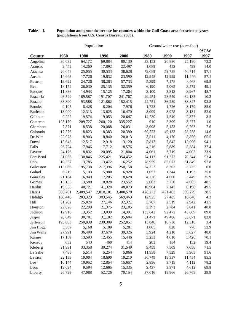
Table 1-1. Population and groundwater use for counties within the Gulf Coast area for selected years (populations from U.S. Census Bureau, 2003).

Population Groundwater use (acre-feet)

County 1950 1980 1990 2000 1980 1990 1997 %GW 1997

Angelina 36,032 64,172 69,884 80,130 33,152 26,886 25,186 73.2 Aransas 2,452 14,260 17,892 22,497 1,089 452 499 14.0 Atacosa 20,048 25,055 30,533 38,628 79,089 59,738 50,714 97.1 Austin 14,663 17,726 19,832 23,590 12,948 12,999 11,446 87.1 Bastrop 19,622 24,726 38,263 57,733 5,399 7,178 8,468 69.8 Bee 18,174 26,030 25,135 32,359 6,190 5,065 3,572 49.1 Bosque 11,836 14,943 15,125 17,204 3,100 3,813 3,967 48.7 Brazoria 46,549 169,587 191,707 241,767 49,454 28,559 32,133 10.2 Brazos 38,390 93,588 121,862 152,415 24,751 36,239 33,847 93.8 Brooks 9,195 8,428 8,204 7,976 1,723 1,726 3,179 85.0 Burleson 13,000 12,313 13,625 16,470 8,099 8,975 3,134 52.0 Calhoun 9,222 19,574 19,053 20,647 14,730 4,549 2,377 3.5 Cameron 125,170 209,727 260,120 335,227 910 2,309 3,277 1.0 Chambers 7,871 18,538 20,088 26,031 3,998 5,153 9,763 7.6 Colorado 17,576 18,823 18,383 20,390 69,522 49,133 28,258 14.6 De Witt 22,973 18,903 18,840 20,013 3,511 4,170 3,856 65.5 Duval 15,643 12,517 12,918 13,120 5,812 7,842 15,096 94.1 Falls 26,724 17,946 17,712 18,576 4,216 5,889 3,384 37.4 Fayette 24,176 18,832 20,095 21,804 4,061 3,719 4,002 23.9 Fort Bend 31,056 130,846 225,421 354,452 74,113 91,373 70,344 53.4 Frio 10,357 13,785 13,472 16,252 78,959 85,073 61,849 97.8 Galveston 113,066 195,738 217,396 250,158 24,322 8,203 5,735 6.0 Goliad 6,219 5,193 5,980 6,928 1,057 1,344 1,193 25.0 Gonzales 21,164 16,949 17,205 18,628 4,226 4,660 3,449 35.9 Grimes 15,135 13,580 18,828 23,552 2,662 3,750 4,665 48.5 Hardin 19,535 40,721 41,320 48,073 10,904 7,145 6,198 49.5 Harris 806,701 2,409,547 2,818,101 3,400,578 428,272 421,463 339,279 38.5 Hidalgo 160,446 283,323 383,545 569,463 12,925 27,485 16,840 4.3 Hill 31,282 25,024 27,146 32,321 3,767 2,519 2,942 41.5 Houston 22,825 22,299 21,375 23,185 2,393 2,784 3,041 48.8 Jackson 12,916 13,352 13,039 14,391 135,642 92,472 43,609 89.8 Jasper 20,049 30,781 31,102 35,604 51,471 49,486 53,071 82.8 Jefferson 195,083 250,938 239,389 252,051 15,046 10,736 12,318 3.4 Jim Hogg 5,389 5,168 5,109 5,281 1,065 828 770 52.9 Jim Wells 27,991 36,498 37,679 39,326 5,924 4,210 3,627 48.0 Karnes 17,139 13,593 12,455 15,446 3,233 4,610 3,426 70.1 Kenedy 632 543 460 414 283 154 132 19.4 Kleberg 21,991 33,358 30,274 31,549 9,459 7,509 7,058 71.5 La Salle 7,485 5,514 5,254 5,866 11,938 7,529 5,965 91.6 Lavaca 22,159 19,004 18,690 19,210 30,749 19,337 11,454 85.5 Lee 10,144 10,952 12,854 15,657 2,856 3,719 4,112 78.2 Leon 12,024 9,594 12,665 15,335 2,437 3,571 4,612 69.8 Liberty 26,729 47,088 52,726 70,154 37,016 19,966 26,765 29.9

7

Table 1-1. Continued.

Population Groundwater use (acre-feet)

County 1950 1980 1990 2000 1980 1990 1997 %GW 1997

Live Oak 9,054 9,606 9,556 12,309 4,526 5,997 6,845 75.0 Madison 7,996 10,649 10,931 12,940 2,199 2,672 2,836 80.7 Matagorda 21,559 37,828 36,928 37,957 38,554 37,537 14,413 9.4 McLennan 130,194 170,755 189,123 213,517 13,017 12,588 15,091 25.7 McMullen 1,187 789 817 851 624 396 858 65.2 Milam 23,585 22,732 22,946 24,238 4,376 18,382 34,405 68.0 Montgomery 24,504 127,222 182,201 293,768 20,828 28,198 40,925 92.1 Nacogdoches 30,326 46,786 54,753 59,203 7,411 8,370 9,389 75.8 Newton 10,832 13,254 13,569 15,072 2,850 3,486 3,072 81.8 Nueces 165,471 268,215 291,145 313,645 2,862 842 3,180 3.4 Orange 40,567 83,838 80,509 84,966 20,638 18,603 17,954 23.9 Polk 16,194 24,407 30,687 41,133 4,306 4,434 5,158 71.3 Refugio 10,113 9,289 7,976 7,828 1,821 1,360 1,271 79.0 Robertson 19,908 14,653 15,511 16,000 20,613 21,364 19,084 87.3 Sabine 8,568 8,702 9,586 10,469 1,061 1,030 909 40.6 San Augustine 8,837 8,785 7,999 8,946 864 651 620 31.6 San Jacinto 7,172 11,434 16,372 22,246 1,512 2,013 2,453 89.7 San Patricio 35,842 58,013 58,749 67,138 4,091 3,163 2,328 11.5 Starr 13,948 27,266 40,518 53,597 677 1,515 1,393 2.4 Trinity 10,040 9,450 11,445 13,779 1,461 1,201 1,430 51.3 Tyler 11,292 16,223 16,646 20,871 2,383 2,193 2,645 95.2 Victoria 31,241 68,807 74,361 84,088 39,933 29,222 27,339 48.5 Walker 20,163 41,789 50,917 61,758 9,867 5,499 6,624 56.3 Waller 11,961 19,798 23,389 32,663 30,692 32,645 27,723 94.6 Washington 20,542 21,998 26,154 30,373 1,848 2,469 2,620 40.0 Webb 56,141 99,258 133,239 193,117 857 1,158 1,526 3.4 Wharton 36,077 40,242 39,955 41,188 175,210 162,820 178,219 53.7 Willacy 20,920 17,495 17,705 20,082 573 17 18 0.1 Wilson 14,672 16,756 22,650 32,408 9,663 15,898 16,585 81.2 Zapata 4,405 6,628 9,279 12,182 242 80 51 0.7 Total 2,920,144 5,751,743 6,706,372 8,268,783 1,708,032 1,580,123 1,385,576 29.7

%GW = percent of total water use in 1997 that was met with groundwater. Groundwater use includes use from all aquifers, including those not discussed in this paper.

In 1997, about one-third of the region’s water supply came from groundwater, and 31 counties obtained more than 60 percent of their water supply from groundwater (Table 1-1). The region withdrew about 1.7 million acre-feet in 1980 and about 1.4 million acre-feet in 1997.

8

Aquifers of the Gulf Coast The Gulf Coast area includes the Gulf Coast, Yegua-Jackson, and Brazos River Alluvium aquifers (Figure 1-5). The boundaries of these aquifers have been defined by the TWDB. Based on the quantity of water supplied by each aquifer, the TWDB has designated the Gulf Coast aquifer as a major aquifer and the Yegua-Jackson and Brazos River Alluvium aquifers as minor aquifers (Ashworth and Hopkins, 1995; TWDB, 2002). Additional water may be produced in smaller, localized aquifers not recognized by the TWDB.

Figure 1-5. Location of major and minor aquifers recognized by the TWDB in the Gulf Coast region that are discussed in this paper and report (delineations from TWDB; this map does not show all aquifers in the upland areas).

9

Groundwater studies have focused primarily on the major aquifers, but additional research has also addressed the minor aquifers. Below are brief descriptions of each of the three recognized aquifers in the Gulf Coast area—more detailed information on these aquifers is available throughout this report.

Gulf Coast Aquifer

The Gulf Coast aquifer is located along the Gulf of Mexico coast throughout all or parts of Aransas, Austin, Bee, Brazoria, Brazos, Brooks, Calhoun, Cameron, Chambers, Colorado, De Witt, Duval, Fayette, Fort Bend, Galveston, Gonzales, Goliad, Grimes, Hardin, Harris, Hidalgo, Jim Hogg, Jim Wells, Jackson, Jasper, Jefferson, Karnes, Kenedy, Kleberg, Lavaca, Liberty, Live Oak, Matagorda, McMullen, Montgomery, Newton, Nueces, Orange, Polk, Refugio, San Jacinto, Sabine, San Patricio, Starr, Trinity, Tyler, Victoria, Walker, Waller, Washington, Webb, Wharton, Willacy, and Zapata counties.

The aquifer has been divided into four units, each of which can be generally correlated to different sedimentary formations (Baker, 1979) and has different hydraulic properties (Chowdhury and Mace, 2003; Chowdhury and others, 2004; Kasmarek and Robinson, 2004). The deepest of these is the Catahoula confining system, which includes the Frio Formation, the Anahuac Formation, and the Catahoula Tuff or Sandstone. The Catahoula is overlain by the Jasper aquifer, which consists of the Oakville Sandstone and Fleming Formation. The upper part of the Fleming Formation forms the Burkeville confining system. This separates the Jasper aquifer from the Evangeline aquifer, which is made up of water within the Goliad Sand. The shallowest unit, the Chicot aquifer, is made up of the Willis Sand, the Bentley and Montgomery formations, the Beaumont Clay, and alluvial deposits at the surface (Baker, 1979). The total sand thickness in all four units ranges from 700 feet in the south to 1,300 feet in the north (Ashworth and Hopkins, 1995).

Groundwater quality in the Gulf Coast aquifer is generally good northeast of the San Antonio River but declines to the southwest due to increased chloride concentrations and saltwater encroachment near the coast. In addition, heavy pumpage has caused saltwater intrusion to occur along the coast as far north as Orange County (Ashworth and Hopkins, 1995). Pumping from the Gulf Coast aquifer between 1985 and 2000 ranged from around 1 million to 1.3 million acre-feet per year. Water level declines of up to 350 feet in Harris, Galveston, Fort Bend, Jasper, and Wharton counties have led to land-surface subsidence (Kasmarek and Robinson, 2004), which is discussed in Chapter 7 of this report. For further information on the Gulf Coast aquifer, see chapters 2, 5, 6, 10, 12, and 16 of this report.

Yegua-Jackson Aquifer

The Yegua-Jackson aquifer runs approximately parallel to the Gulf of Mexico coastline, approximately 100 miles inland, and is located in all or parts of Angelina, Atascosa, Bastrop, Brazos, Burleson, Duval, Fayette, Frio, Gonzales, Grimes, Houston, Jasper, Jim Hogg, Karnes, LaSalle, Lavaca, Lee, Leon, Live Oak, Madison, McMullen, Nacogdoches, Newton, Polk, Sabine, San Augustine, Starr, Trinity, Tyler, Walker, Washington, Webb, Wilson, and Zapata

10

counties. It includes water contained in Tertiary deposits of sand, silt and clay that form the Yegua Formation and the Jackson Group (TWDB, 2002). The aquifer is separated from the overlying Gulf Coast aquifer by the Catahoula Sandstone and divided from the underlying Sparta aquifer by the clay-rich Cook Mountain Formation. The aquifer is approximately 15 to 40 miles wide and is found between the Gulf Coast aquifer to the southeast and the Sparta aquifer to the northwest.

From 1980 to 1997, between approximately 11,000 and 14,000 acre-feet of water was withdrawn from the Yegua-Jackson aquifer. Most withdrawals take place where other aquifers are not present or where the cost of pumping from other aquifers is comparatively high. To learn more about this aquifer, see Chapter 3 of this report.

Brazos River Alluvium

The Brazos River Alluvium aquifer is located in parts of Austin, Bosque, Brazos, Burleson, Falls, Fort Bend, Grimes, Hill, McLennan, Milam, Robertson, Waller, and Washington counties. It consists of water-bearing sediments, primarily gravel and sand, within the floodplain and terrace deposits of the Brazos River. The deposits reach up to 100 feet thick in some places and up to 8 miles wide, with the thickness generally widening and thickening towards the coast. Water quality in the aquifer is typically hard, and the concentration of dissolved solids in the water varies and can reach more than 1,500 milligrams per liter. The Brazos River Alluvium aquifer is hydraulically connected to the Brazos River as well as to underlying bedrock aquifers, including the Yegua-Jackson and Gulf Coast aquifers (Cronin and Wilson, 1967).

Most water is found in the alluvium within the floodplain. The primary use of water pumped from the aquifer is for irrigation. Between 1980 and 1997, withdrawals from the aquifer typically ranged between 20,000 and 40,000 acre-feet per year. Chapter 4 provides a more detailed description of the Brazos River Alluvium aquifer and discusses a model created to simulate the conjunctive use water stored in the aquifer with surface water in the Brazos River.

Groundwater Issues in the Gulf Coast Region The people of the Texas Gulf Coast have to consider a wide variety of issues that can affect their groundwater. Some of these are common throughout the state, and some are unique to the region. Below are brief descriptions of topics related to groundwater in the region that are addressed in more detail in other chapters of this report.

Groundwater Quality

Water quality often determines whether or not water can be used for drinking, industry, irrigation, or other uses. The salinity—or amount of dissolved solids—of groundwater in the aquifer increases naturally in deep parts of the Gulf Coast aquifer, toward the coast. In addition, the southern part of the aquifer contains significantly higher amounts of chloride, sulfate, and sodium than the northern part. The presence of arsenic, radium, and many other constituents that

11

are found in the Gulf Coast aquifer and that affect water quality is described and analyzed in detail in Chapter 5.

Subsidence

Land-surface subsidence has been a persistent problem in the Harris, Galveston, and Fort Bend counties for several decades. As water is withdrawn from deep, confined portions of the Gulf Coast aquifer, the hydraulic pressure on the sediments decreases. This causes the de-watered sediments to compact due to the weight of overlying sediments. If pumping rates are low, this will have little effect, because sand layers are dewatered first and these compact only slightly. However, if pumping continues, water will start to be drawn from less transmissive clay layers. While sand grains are fairly round, clay grains are sheet-like. As they become de-watered and compacted, they align perpendicular to the load applied by overlying sediments. As clay grains line up in the same direction, the porosity and thickness of the clay layer decreases. (For a very rough comparison, imagine the difference in thickness between a house of cards—with cards balanced and aligned at different directions—and the same cards aligned flat on the ground.) Even if the layer is saturated with water again, about 90 percent of this compaction is permanent (Kasmarek and Robinson, 2004). To read more about how land-surface subsidence has affected the northern Gulf Coast region of Texas and how Texans have worked to combat the problem, see Chapter 7 of this report.

Drought

Drought can affect groundwater supplies in many ways—low precipitation levels can lead to reduced recharge to the aquifer and increased pumping by users. Records of precipitation in the Gulf Coast region go back as far as the mid-1800s in some places, allowing a long-term look at the frequency and duration of drought in the area.

The Palmer Drought Severity Index, which is the most commonly used drought index in Texas and the rest of the U.S., and the Standardized Precipitation Index, which can measure drought over time scales varying from three months to four years, are two systems that have been created to quantify drought. Using these indexes, Chapter 8 describes historical drought events in different parts of the Gulf Coast region.

Groundwater Flow and Estuaries

Estuaries, or coastal bays that are influenced by tides and freshwater inputs, often have high biological productivity and are of environmental and economic importance. Estuarine ecosystems cover more than 2.6 million acres along the Gulf Coast of Texas. The economy of the region depends on these areas for navigation, minerals, fisheries, recreation, and natural waste treatment. The total value of these services to the residents of the region is in the billions of dollars (TWDB, 2005).

Surface water discharge at the coast has long been known to affect the chemistry and ecology of estuaries. In the Gulf Coast region of Texas, TWDB and Texas Parks and Wildlife Department

12

have been studying freshwater inflows from surface water into estuaries for over twenty years. Groundwater discharge to the ocean, on the other hand, is much more difficult to see or measure and has undergone much less study in Texas and in much of the world. Researchers are starting to find that groundwater can constitute a significant amount of freshwater flow to coastal areas and may have important impacts on coastal areas, including estuaries. See Chapter 9 of this report for a discussion of how groundwater discharge to coasts is currently understood and being studied.

Salt Domes

As the sediments that now make up the Gulf Coast aquifer were being deposited, underlying evaporite (salt-rich) deposits were deformed. In some areas, this deformation resulted in the upwelling of salt domes into the overlying sediments. These domes are one to three miles in diameter and are composed almost entirely of crystalline rock salt covered by a cap rock of sulfate and carbonate minerals.

The 38 salt domes that are found within the Gulf Coast aquifer in Texas provide natural resources such as oil, gas, salt, and sulfur, and have been used for storing petroleum products. However, the development of salt domes can lead to the formation of sinkholes and creates a potential for groundwater contamination. Despite these risks, there has been little data collection or research over the past twenty years to address how salt dome development may affect the Gulf Coast aquifer. Chapter 12 of this report describes salt domes in more detail and summarizes what is known about salt domes and hydrogeology.

Brackish Groundwater Desalination

As demand for water in Texas grows, additional sources of water are being sought, in particular to provide adequate supplies in times of drought. Desalination technology offers a way to use the large amounts of water that are available in aquifers but are too saline for normal use. Brackish desalination plants remove dissolved solids from groundwater using processes such as filtration, reverse osmosis, and electrodialysis reversal.

Brackish groundwater desalination offers a promising water resource option for the Gulf Coast region. The Gulf Coast aquifer contains about one-fifth of the estimated quantity of brackish groundwater that is suitable for desalination in Texas. As desalination is becoming more cost effective, plants are being built, planned, and incorporated into the water management strategies of regional water planning groups in the area. For more information, see Chapters 13 and 14.

Oil and Gas Production

For over 150 years, oil and gas development in Texas has co-existed with groundwater use. As these resources were developed, so too did the risk that hydrocarbon extraction would lead to the contamination of groundwater resources. For example, products used in and created by production can contaminate groundwater through pipeline leaks, accidental spills, or produced water of poor quality.

13

The Railroad Commission of Texas is the state agency with the authority and responsibility to regulate oil and gas operations, in part to protect groundwater resources. More information about the regulation of oil and gas production to protect groundwater supplies can be found in Chapter 15 of this report.

Historical and Future Production of the Gulf Coast Aquifer

One-third of the state’s population lives in counties where the Gulf Coast aquifer is found. More water is pumped from the Gulf Coast aquifer in Texas than from any of the state’s other aquifers except for the Ogallala. Thus, production in the Gulf Coast aquifer is a topic of interest for many people who are concerned with the quality of life and the economy in the state. Chapter 16 describes the history and future of groundwater development from the Gulf Coast aquifer, including information on past pumping statistics and development projects currently under consideration.

Groundwater Management

Several chapters of this report discuss various aspects of groundwater management in the Gulf Coast region of Texas. Chapter 11 describes optimization models, which can be used by decision-makers to maximize or minimize specific constraints, such as maintaining a certain level of springflow, based on their goals. It then considers how the groundwater availability models (GAMs) developed by the TWDB can be used along with optimization models to help make groundwater management decisions. Chapter 17 provides one perspective on how the scientific and legal framework for groundwater management in the Texas Gulf Coast relates to the values held by individuals that shape the state’s localized form of groundwater management. It then gives some ideas for how to promote understanding and cooperation between stakeholders. Chapter 20 gives information on groundwater management through groundwater conservation districts.

Local Studies

As demand for water increases and new groundwater development projects are considered, public and private groups are conducting detailed local studies of the hydrogeology in the Gulf Coast region. The results of these studies help to predict whether a project will meet its goals and maximize the success of the project.

Several chapters in this report discuss the results of such studies. Chapter 4 describes a groundwater model of the Brazos River Alluvium aquifer that was created to help assess the possibility of temporarily storing extra water in the aquifer during wet periods to use during times of low precipitation and river flow. Chapter 6 and the extended abstracts in chapters 18 and 19 describe several studies that are being done to plan for the Lower Colorado River Authority-San Antonio Water System Water Project. These studies look at the geology and hydraulic properties of the Gulf Coast aquifer, recharge to the Gulf Coast aquifer, and interactions between the Gulf Coast aquifer and the rivers that cross it.

14

Regional Water Planning In 1997, the Texas Legislature enacted Senate Bill 1, a comprehensive water legislation created to plan for managing water resources as the population and water demand of Texas grows. This bill calls for a “bottom up” planning process, creating sixteen regional water planning areas and corresponding regional water planning groups. Each regional water planning group is formed by members representing 11 different interest groups, including agriculture, counties, the environment, industries, municipalities, the public, river authorities, small business, steam-electric generating facilities, water districts, and water utilities located within the regional water planning area, as well as additional entities chosen by the regional water planning groups.

It is the responsibility of each of the regional water planning groups to create a regional water plan for its region that defines current and projected water supplies and water demand and shows how the region plans to meet future water supply needs and respond to drought. These regional water plans were submitted to the TWDB in January of 2001 for the first round of regional water planning. The TWDB used these individual plans to create a comprehensive state water plan, which it released in January of 2002. Most of the regional water plans for 2006 were submitted to TWDB in January of 2006 for the second round of regional water plans. The next state water plan will be released in January of 2007. These regional and state plans are available on the TWDB website at www.twdb.state.tx.us. In order to respond to changes in the regional water planning areas, the water plans will be updated every five years. Financial assistance from the TWDB and water right permits from the Texas Commission on Environmental Quality will only be provided if the purpose of the project or permit is consistent with the state water plan.

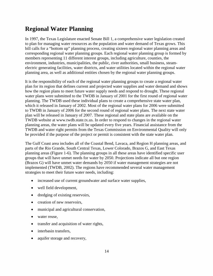
The Gulf Coast area includes all of the Coastal Bend, Lavaca, and Region H planning areas, and parts of the Rio Grande, South Central Texas, Lower Colorado, Brazos G, and East Texas planning areas (Figure 1-6). The planning groups in all these areas have identified specific user groups that will have unmet needs for water by 2050. Projections indicate all but one region (Brazos G) will have unmet water demands by 2050 if water management strategies are not implemented (TWDB, 2002). The regions have recommended several water management strategies to meet their future water needs, including:

• increased use of current groundwater and surface water supplies,

• well field development,

• dredging of existing reservoirs,

• creation of new reservoirs,

• municipal and agricultural conservation,

• water reuse,

• transfer and acquisition of water rights,

• interbasin transfers,

• aquifer storage and recovery,

15

• desalination,

• rainwater harvesting,

• brush management, and

• weather modification (TWDB, 2002).

Figure 1-6. Location of regional water planning areas in the Gulf Coast region.

16

Groundwater Conservation Districts Since 1904, Texas has governed groundwater use through the Rule of Capture. This rule allows landowners to pump as much groundwater as they like, so long as the purpose of pumping is not “malice or willful waste” and not be held liable if neighbors complain that their wells have been depleted by pumping. In order to allow the option of locally controlled groundwater regulation, the Legislature authorized the creation of groundwater conservation districts in 1949 (Mace and others, 2004). Today these districts are recognized by the Legislature as the state’s preferred method of managing groundwater resources. Each groundwater conservation district has the authority to regulate groundwater pumping within its boundaries and must complete a ten-year groundwater management plan every five years, describing how it plans to address relevant groundwater issues such as changes in water use, drought, and water quality.

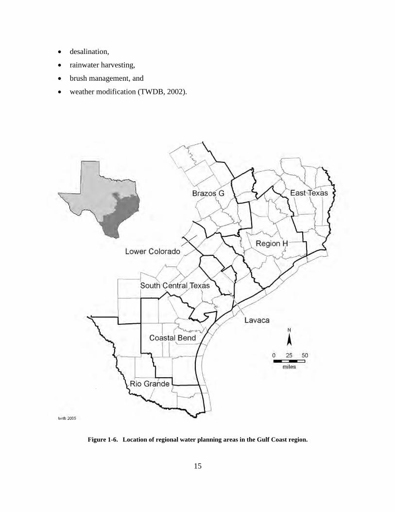
House Bill 1763, passed by the Texas Legislature in 2005, will change the way that groundwater conservation districts manage groundwater. The bill requires that all groundwater conservation districts coordinate their planning efforts with other districts that are located within the same groundwater management area. There are 16 groundwater management areas in Texas, and the Gulf Coast region includes all or part of 7 of them (Figure 1-7).

By the year 2010, the groundwater conservation districts in each groundwater management area will need to establish desired future conditions for aquifers within their groundwater management area boundaries. After this time, the groundwater conservation districts will need to ensure that their management plans are designed to meet the newly decided conditions. The role of the TWDB in this process will be to provide each groundwater conservation district with the estimated amount of managed available groundwater that will be available based on the desired future conditions that are agreed upon within the groundwater management areas. The TWDB will only provide these numbers—the agency will not approve or disapprove of the conditions that the groundwater conservation districts give to them unless the conditions are hydrologically unreasonable.

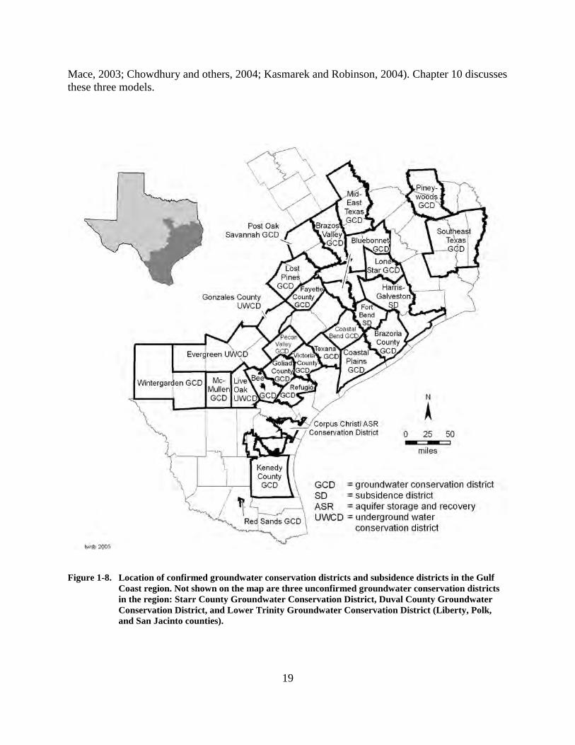
The Gulf Coast area is home to 25 confirmed groundwater conservation districts, as well as 1 aquifer storage and recovery conservation district and 2 subsidence districts (Figure 1-8):

1. Bee Groundwater Conservation District,

2. Bluebonnet Groundwater Conservation District,

3. Brazoria County Groundwater Conservation District,

4. Brazos Valley Groundwater Conservation District,

5. Coastal Bend Groundwater Conservation District,

6. Coastal Plains Groundwater Conservation District,

7. Corpus Christi Aquifer Storage and Recovery Conservation District,

8. Evergreen Underground Water Conservation District,

9. Fayette County Groundwater Conservation District,

17

10. Fort Bend Subsidence District,

11. Goliad County Groundwater Conservation District,

12. Gonzales County Underground Water Conservation District,

13. Harris-Galveston Subsidence District,

14. Kenedy County Groundwater Conservation District,

15. Live Oak Underground Water Conservation District,

16. Lone Star Groundwater Conservation District,

17. Lost Pines Groundwater Conservation District,

18. McMullen Groundwater Conservation District,

19. Mid-East Texas Groundwater Conservation District,

20. Pecan Valley Groundwater Conservation District,

21. Pineywoods Groundwater Conservation District,

22. Post Oak Savannah Groundwater Conservation District,

23. Red Sands Groundwater Conservation District,

24. Refugio Groundwater Conservation District,

25. Southeast Texas Groundwater Conservation District,

26. Texana Groundwater Conservation District,

27. Victoria County Groundwater Conservation District, and

28. Wintergarden Groundwater Conservation District.

At the time of publication, there were three unconfirmed groundwater conservation districts in the region: Starr County Groundwater Conservation District, Duval County Groundwater Conservation District, and Lower Trinity Groundwater Conservation District (Liberty, Polk, and San Jacinto counties).

Groundwater Availability Modeling The development of state-of-the-art, publicly available computer models of groundwater resources in Texas began in 1999, when the Legislature provided initial funding for the TWDB to create groundwater availability models (GAMs) for the major aquifers of Texas. In 2001, the Legislature enacted Senate Bill 2, which directed the TWDB to complete groundwater availability models for the minor aquifers.

A main purpose of these models is to provide regional water planning groups and groundwater conservation districts with information to use in assessing the availability of groundwater in their regions or areas. With information from the models, they can evaluate their social and economic demand for water in relation to the effects of groundwater use on the quantity and quality of groundwater, groundwater flow to springs, land surface subsidence, and other aquifer

18

Figure 1-7. Location of groundwater management areas in the Gulf Coast region.

characteristics. This can help them make more informed decisions on how to manage their groundwater supplies and to meet their current and future demands for water.

Three GAMs have been completed for the Gulf Coast aquifer. In addition, the TWDB will be creating GAMs for the Brazos River Alluvium aquifer and the Yegua Jackson aquifer; however, the schedule is not yet set for their development. Because of the large size of the Gulf Coast aquifer, separate models were created for different portions of the aquifer. A GAM on the lower Rio Grande valley region was completed in October of 2003. The second GAM, covering the central part of the aquifer, was completed in September of 2004. The third GAM, which models the northern part of the aquifer, was also completed in September of 2004. Reports describing these models and how they were developed are available on the TWDB website (Chowdhury and

19

Mace, 2003; Chowdhury and others, 2004; Kasmarek and Robinson, 2004). Chapter 10 discusses these three models.

Figure 1-8. Location of confirmed groundwater conservation districts and subsidence districts in the Gulf Coast region. Not shown on the map are three unconfirmed groundwater conservation districts in the region: Starr County Groundwater Conservation District, Duval County Groundwater Conservation District, and Lower Trinity Groundwater Conservation District (Liberty, Polk, and San Jacinto counties).

20

Summary More than a third of all Texans live in the Gulf Coast region, an area that runs from the Rio Grande Valley in the south to the Sabine River basin in the north. The population has increased dramatically over the last 50 years and with it the demand for water. Many people in the region depend partly or entirely on groundwater to meet their needs. As water users, groundwater conservation districts, and regional water planning groups work to meet their groundwater needs today and plan for the future, a diverse range of issues must be addressed. Among these are the quantity and quality of water in the region’s aquifers, the threat of drought, impacts of pumping such as land subsidence and reduced flow to estuaries, and possible effects of oil and gas production on groundwater supplies. We continue to improve our understanding of these issues through the development of groundwater availability models and through regional studies carried out by public and private groups. In the following chapters, experts from a variety of disciplines and industries offer more detailed information and ideas about all of these topics.

References Ashworth, J. B., and Hopkins, J., 1995, Aquifers of Texas: Texas Water Development Board

Report 345, 69 p.

Baker, E. T., 1979, Stratigraphic and hydrogeologic framework of part of the coastal plain of Texas: Texas Water Development Board Report 236, 43 p.

BEG, 1992, Geologic map of Texas, 1992: Austin, TX, Bureau of Economic Geology, scale 1:500,000.

Chowdhury, A. H., and Mace, R. E., 2003, A groundwater availability model of the Gulf Coast aquifer in the Lower Rio Grande Valley, Texas—Numerical simulations through 2050: Texas Water Development Board Report 171 p.

Chowdhury, A. H., Wade, S., Mace, R. E., and Ridgeway, C., 2004, Groundwater availability model of the central Gulf Coast aquifer system—Numerical simulations through 1999: Texas Water Development Board Report, 163 p.

Cronin, J. G., and Wilson, C. A., 1967, Ground water in the flood-plain alluvium of the Brazos River, Whitney Dam to vicinity of Richmond, Texas: Texas Water Development Board Report 41, 80 p.

Daly, C., 1998, Annual Texas precipitation: Portland, OR, Water and Climate Center of the Natural Resources Conservation Service, GIS shapefile data.

Fenneman, N. M., 1938, Physiography of the eastern United States: New York, NY, McGraw-Hill Book Company, Incorporated, 714 p.

21

Kasmarek, M. C., and Robinson, J. L., 2004, Hydrogeology and simulation of groundwater flow and land-surface subsidence in the northern part of the Gulf Coast aquifer system, Texas: United States Geological Survey Scientific Investigations Report 2004-5102, 111 p.

Larkin, T. J., and Bomar, G. W., 1983, Climatic Atlas of Texas: Texas Department of Water Resources LP-192, 151 p.

Mace, R. E., Ridgeway, C., and Sharp, J. M., Jr., 2004, Groundwater is no longer secret and occult—A historical and hydrogeologic analysis of the East case: in Mullican, W. F., III, and Schwartz, S., eds., 100 years of rule of capture: From East to groundwater management, Texas Water Development Board Report 361, p. 63–88.

TWDB, 2002, Water for Texas—2002: Texas Water Development Board Document GP-7-1, 155 p.

TWDB, 2005, Texas Bays and Estuaries Program: program overview at (http://www.twdb.state. tx.us/data/bays_estuaries/bays_estuary_toc.asp).

U.S. Census Bureau, 2003, Population and housing unit counts, PHC-3-45, Texas: 2000 census of population and housing, Washington, DC, 184 p. Available at (http://www.census.gov/ prod/cen2000/phc-3-45.pdf).

22

This page intentionally blank.

23

Chapter 2

Geology of the Gulf Coast Aquifer, Texas Ali H. Chowdhury, Ph.D., P.G.1 and Mike J. Turco2

Introduction The Gulf Coast aquifer in Texas extends over 430 miles from the Texas-Louisiana border in the northeast to the Texas-Mexico border in the south (Figure 2-1). Over 1.1 million acre-feet of groundwater are annually pumped from this aquifer in Texas. A large portion of this water supply is used for irrigation and drinking water purposes by the fast growing communities along the Texas Gulf Coast.

The geology of the Gulf Coast aquifer in Texas is complex due to cyclic deposition of sedimentary facies. Sediments of the Gulf Coast aquifer were mainly deposited in the coastal plains of the Gulf of Mexico Basin. These sediments were deposited under a fluvial-deltaic to shallow-marine environments during the Miocene to the Pleistocene periods. Repeated sea-level changes and natural basin subsidence produced discontinuous beds of sand, silt, clay, and gravel. Six major sediment dispersal systems that sourced large deltas distributed sediments from erosion of the Laramide Uplift along the Central and southern Rockies and Sierra Madre Oriental (Galloway and others, 2000; Galloway, 2005). Geographic locations of the various fluvial systems remained relatively persistent, but the locations of the depocenters where the thickest sediment accumulations occurred shifted at different times (Solis, 1981). Stratigraphic classification of the Gulf Coast aquifer in Texas is complex and controversial, with more than seven classifications proposed. However, Baker’s (1979) classification based on fauna, electric logs, facies associations, and hydraulic properties of the sediments has received widespread acceptance. Baker (1979) classified the Gulf Coast aquifer into five hydrostratigraphic units. From oldest to youngest, these are: (1) the Catahoula Confining System, (2) the Jasper aquifer, (3) the Burkeville Confining System, (4) the Evangeline aquifer, and (5) the Chicot aquifer.

Numerous growth faults (curved faults that are syndepositional and grow with depth of burial) parallel the Gulf Coast and controlled sediment accumulation and dispersal patterns during deposition. Salt domes are more common in the northern than the southern parts of the Texas Gulf Coast. These salt domes locally penetrate shallow areas of the Gulf Coast aquifer. Rapid burial of the fluvio-deltaic sediments in the Texas Gulf Coast caused the development of overpressure zones in the subsurface. In this paper, we will describe: (1) the evolution of the Gulf of Mexico basin and associated sediments of the Texas Gulf Coast aquifer; (2) structural

1 Texas Water Development Board 2 U.S. Geological Survey Texas Water Science Center

24

Figure 2-1. Extent of the Gulf Coast aquifer, major rivers, and cities along the Texas Gulf Coast.

features including faults, salt domes, and overpressure zones; (3) depositional environments; and (4) the stratigraphy of the Gulf Coast aquifer in Texas. We briefly describe geologic relationships to the occurrences of groundwater and petroleum resources in the Texas Gulf Coast.

Physiography The Gulf Coast aquifer in Texas is mainly covered by a smooth, low-lying coastal plain that gradually rises from sea level in the east to as much as 900 feet in the north and the west (Figure 2-2). The coastal uplands end at the contact of the Cretaceous clay and limestone where elevations rise sharply (Figure 2-2). The surficial geology of the Texas Gulf Coast is complex,

25

Figure 2-2. Land surface elevation of the area directly overlying the Gulf Coast aquifer in Texas (from Texas General Land Office, http://www.glo.state.tx.us/gisdata/jpgs/elev.jpg).

consisting of a mosaic of lithofacies with the Pleistocene and Holocene sediments covering most of the outcrop areas (Figure 2-3). The Coastal Plain is underlain by a massive thickness of sediments that form a homocline sloping gently towards the Gulf of Mexico. Several major rivers dissect the Gulf Coast aquifer and flow nearly perpendicular to the Gulf of Mexico. These rivers include the Sabine, Trinity, Colorado, Guadalupe, Brazos, San Antonio, and Rio Grande (Figure 2-1). Between the valleys of the major rivers crossing the coastal plains, differential erosion of the softer and harder beds led to the formation of parallel low ridges and escarpments. These features provided the lowlands with a distinctive topographic belt. This “belted”

26

Figure 2-3. Surficial geology of the Gulf Coast aquifer in Texas (Aronow and Barnes, 1968; Shelby and others, 1968; Proctor and others, 1974; Aronow and others, 1975; Aronow and Barnes, 1975; Brewton and others, 1976a; Brewton and others, 1976b).

topography is better developed in East Texas and is less evident in South Texas due to increased aridity and the influence of the Sierra Madre Oriental in Mexico (Bryant and others, 1991). Most of the major rivers that arise farther away from the coastal plains have broad alluvial valleys and deltaic plains and empty sediment loads directly into the Gulf of Mexico. The smaller rivers have narrow valleys and drain into estuaries or lagoons that are disconnected from the Gulf by onshore barrier islands or offshore bars. Long barrier islands with few tidal inlets and adjoining lagoons parallel part of the Texas Gulf Coast. Padre Island, with a length of about 130 miles, is the longest barrier island adjacent to the Gulf of Mexico.

27

The Gulf Coast aquifer in Texas outcrops over a large geographic area located between 18°N and 31°N latitudes. Therefore, the climate varies widely, from humid in the north to semi-tropical to semi-arid in the south. Annual rainfall ranges from about 56 inches in the north to about 18 inches in the south. The mean annual temperature ranges from about 60° F in the north to about 70° F in the south. Annual pan evaporation rates range from about 60 inches in the north to 100 inches in the south (Williamson and Grubb, 2001).

Basin evolution and structural features Sediments of the Texas Gulf Coast aquifer were deposited in the coastal plains of the Gulf of Mexico Basin (Figure 2-4) during the Tertiary and Quaternary periods. The Gulf of Mexico Basin was formed by the downfaulting and downwarping of Paleozoic basement rocks during the break-up of the Paleozoic megacontinent Pangaea and the opening of the North Atlantic Ocean in the Late Triassic (Byerly, 1991; Hosman and Weiss, 1991). Igneous processes played a significant part in the evolution of the Gulf of Mexico basin, as observed from the presence of

Figure 2-4. Geographic extent of the Gulf of Mexico Basin (from Salvador, 1991).

28

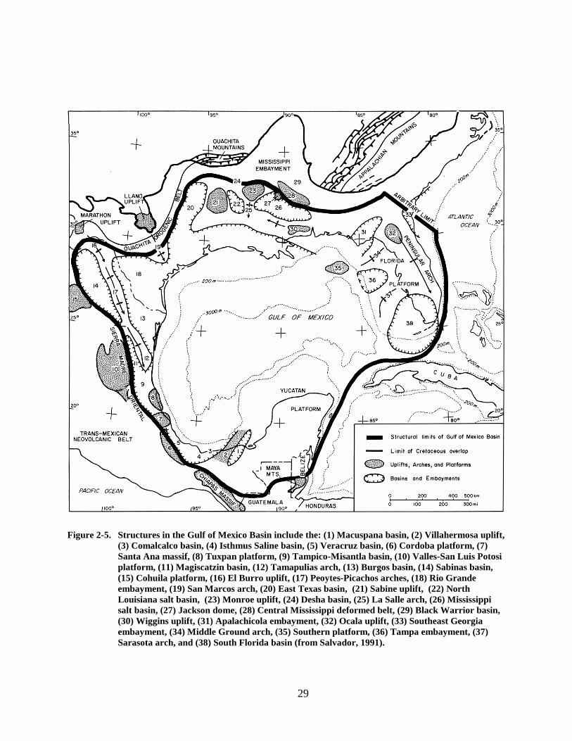
basaltic rocks in rift basins around the Gulf of Mexico margins. Igneous processes may have partly controlled thermal and uplift history of the Gulf of Mexico basin (Byerly, 1991). Most of the igneous activity occurred in the Late Cretaceous and Oligocene-Miocene periods, although activity continues today in the western part of the Gulf of Mexico basin in Mexico (Byerly, 1991). Local structures that rim the Gulf of Mexico basin are primarily formed by gravity acting on thick sedimentary sections deposited on abnormally pressured shale or salt that sole out above the basement to produce salt-flow structures and growth faults (Figure 2-5) (Nelson, 1991).

The Balcones and Luling-Mexia-Talco fault zones rim the basin and form a divide between Upper Cretaceous and Eocene strata (Figure 2-6) (McCoy, 1990). The Balcones fault zone is dominated by normal faults that run parallel to the trend of the Ouachita orogenic belt. Along these faults, sediments have been displaced up to 1,500 feet, shifting downward toward the Gulf of Mexico. Where the faults juxtapose against the resistant Lower Cretaceous and more resistant Upper Cretaceous sediments, it forms the Balcones Escarpment (Ewing, 1991). The Luling-Mexia-Talco fault system consists of three segments of symmetric grabens linked by deep en-echelon normal faults and extends from Central Texas to the Arkansas border (Ewing, 1991). Movement along the faults began in the Jurassic, as evidenced by thick sediment piles in the grabens, and continued later movement is supported by offsets of Paleocene beds. Many of the local structures, including the Sabine Arch, Houston Embayment, San Marcos Arch, Rio Grande Embayment, salt domes, and numerous northeast-southwest trending growth faults, began to form prior to the Tertiary period (Figure 2-5). The growth faults have an extensional component and are often referred to as listric-normal faults (listric from Greek for “shovel” to describe curved fault planes) (Figures 2-7 and 2-8) (Nelson, 1991). Bornhauser (1958) suggested that most of the regional structures, embayments, arches, and flexures were created by a combination of differential subsidence of the basin floor and thick sediments that flowed as viscous fluids on sloping surfaces. Others suggested that deep-seated vertical intrusions of salt in the form of narrow ridges pushed up the gulf-ward dipping beds to form deep-seated anticlines (Quarles, 1952; Cloos, 1962). These structural features controlled sediment accumulation patterns, as supported by the observation that bedding commonly thins towards and over the arches and thickens in the embayments (Grubb, 1998). All regional and local structures in the Texas Gulf Coast were developed by shallow tectonics in rapidly subsiding basins, which caused sediments to be buried to considerable depths (Bornhauser, 1958) while still preserving most of their initial porosity. If the sediments were affected by deeper tectonic events, a higher temperature associated with metamorphic processes would have destroyed most of the transmissive capacities of the sandstone.

The Sabine Arch lies between the East Texas and North Louisiana basins (Figure 2-5), and its boundaries are gentle homoclines into the surrounding basins. The uplifted area contains a thin layer of Jurassic salt that forms low amplitude swells (Ewing, 1991). In the mid-Cretaceous, the Sabine Uplift area was uplifted and subsequently eroded to form the clastic sediments of the Woodbine Formation. The Woodbine Formation was uplifted again and the sediments were subsequently eroded and deposited before the formation of the Austin Chalk (Halbouty and Halbouty, 1982). A third episode of uplift during the Eocene provided the current outcrop pattern around the Sabine arch (Ewing, 1991).

The San Marcos arch is a broad area of lesser subsidence and is a subsurface extension of the Llano Uplift, which contains exposed Precambrian Rocks. The arch is located between the Rio

29

Figure 2-5. Structures in the Gulf of Mexico Basin include the: (1) Macuspana basin, (2) Villahermosa uplift, (3) Comalcalco basin, (4) Isthmus Saline basin, (5) Veracruz basin, (6) Cordoba platform, (7) Santa Ana massif, (8) Tuxpan platform, (9) Tampico-Misantla basin, (10) Valles-San Luis Potosi platform, (11) Magiscatzin basin, (12) Tamapulias arch, (13) Burgos basin, (14) Sabinas basin, (15) Cohuila platform, (16) El Burro uplift, (17) Peoytes-Picachos arches, (18) Rio Grande embayment, (19) San Marcos arch, (20) East Texas basin, (21) Sabine uplift, (22) North Louisiana salt basin, (23) Monroe uplift, (24) Desha basin, (25) La Salle arch, (26) Mississippi salt basin, (27) Jackson dome, (28) Central Mississippi deformed belt, (29) Black Warrior basin, (30) Wiggins uplift, (31) Apalachicola embayment, (32) Ocala uplift, (33) Southeast Georgia embayment, (34) Middle Ground arch, (35) Southern platform, (36) Tampa embayment, (37) Sarasota arch, and (38) South Florida basin (from Salvador, 1991).

30

Figure 2-6. Map showing locations of faults in the Gulf Coast aquifer in Texas. Note that most of the faults have extensional components and occur parallel to the coast. Only structural features for Texas are shown (modified from Murray, 1961 and Hosman, 1996).

Grande Embayment and East Texas Basin (Figure 2-5). The arch is crossed by the basement involved normal faults of the Balcones-Lulling fault zone that parallels the buried Ouachita Orogenic Belt (Ewing, 1991).

The Rio Grande embayment is a small deformed basin showing signs of compression during the Laramide orogeny in the Late Cretaceous–Paleogene. The embayment lies between El Burro uplift in Northeast Mexico and the south of the basin-marginal Balcones fault zone (Figure 2-5) (Ewing, 1991). It contains few Jurassic salt domes, but salt tectonics is a minor component of the basin history. Jurassic and Cretaceous sedimentation were continuous and recorded a general subsidence and transgression in the Early Cretaceous (Ewing, 1991).

31

Figure 2-7. Diagrammatic cross-section along the central part of the Texas Gulf Coast and northern Gulf of Mexico basin showing depositional and structural styles exhibited by fluvial-deltas (from Bruce, 1973 and Solis, 1981).

Figure 2-8. An example of a growth fault in the Gulf Coast across Corsair fault trend, offshore Texas. This seismic section shows a listric segment of the fault (A), a bedding parallel slide surface that rests on overpressured shale (B), and a deep ramp that changes orientation of the slide surface (from Vogler and Robinson, 1987). Reprinted by permission of the AAPG whose permission is required for further use.

32

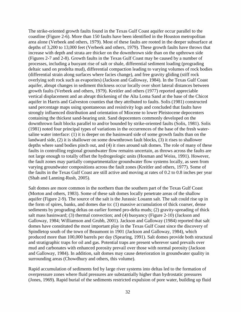
The strike-oriented growth faults found in the Texas Gulf Coast aquifer occur parallel to the coastline (Figure 2-6). More than 150 faults have been identified in the Houston metropolitan area alone (Verbeek and others, 1979). Most of these faults are rooted in the deeper subsurface at depths of 3,200 to 13,000 feet (Verbeek and others, 1979). These growth faults have throws that increase with depth and strata are thicker on the downthrown side than on the upthrown side (Figures 2-7 and 2-8). Growth faults in the Texas Gulf Coast may be caused by a number of processes, including a buoyant rise of salt or shale, differential sediment loading (prograding deltaic sand on prodelta mud), differential compaction leading to varying volumes of rock bodies (differential strain along surfaces where facies change), and free gravity gliding (stiff rock overlying soft rock such as evaporites) (Jackson and Galloway, 1984). In the Texas Gulf Coast aquifer, abrupt changes in sediment thickness occur locally over short lateral distances between growth faults (Verbeek and others, 1979). Kreitler and others (1977) reported appreciable vertical displacement and an abrupt thickening of the Alta Loma Sand at the base of the Chicot aquifer in Harris and Galveston counties that they attributed to faults. Solis (1981) constructed sand percentage maps using spontaneous and resistivity logs and concluded that faults have strongly influenced distribution and orientation of Miocene to lower Pleistocene depocenters containing the thickest sand-bearing unit. Sand depocenters commonly developed on the downthrown fault blocks parallel to and/or bounded by strike-oriented faults (Solis, 1981). Solis (1981) noted four principal types of variations in the occurrences of the base of the fresh water-saline water interface: (1) it is deeper on the basinward side of some growth faults than on the landward side, (2) it is shallower on some downthrown fault blocks, (3) it rises to shallower depths where sand bodies pinch out, and (4) it rises around salt domes. The role of many of these faults in controlling regional groundwater flow remains uncertain, as throws across the faults are not large enough to totally offset the hydrogeologic units (Hosman and Weiss, 1991). However, the fault zones may partially compartmentalize groundwater flow systems locally, as seen from varying groundwater compositions across the fault zones (Kreitler and others, 1977). Some of the faults in the Texas Gulf Coast are still active and moving at rates of 0.2 to 0.8 inches per year (Shah and Lanning-Rush, 2005).

Salt domes are more common in the northern than the southern part of the Texas Gulf Coast (Morton and others, 1983). Some of these salt domes locally penetrate areas of the shallow aquifer (Figure 2-9). The source of the salt is the Jurassic Louann salt. The salt could rise up in the form of spires, banks, and domes due to: (1) massive accumulation of thick coarser, dense sediments by prograding deltas on earlier formed pro-delta muds; (2) gravity-spreading of thick salt mass basinward; (3) thermal convection; and (4) buoyancy (Figure 2-10) (Jackson and Galloway, 1984; Williamson and Grubb, 2001). Jackson and Galloway (1984) reported that salt domes have constituted the most important play in the Texas Gulf Coast since the discovery of Spindletop south of the town of Beaumont in 1901 (Jackson and Galloway, 1984), which produced more than 100,000 barrels per day (Spearing, 1991). Salt domes provide both structural and stratigraphic traps for oil and gas. Potential traps are present wherever sand prevails over mud and carbonates with enhanced porosity prevail over those with normal porosity (Jackson and Galloway, 1984). In addition, salt domes may cause deterioration in groundwater quality in surrounding areas (Chowdhury and others, this volume).

Rapid accumulation of sediments fed by large river systems into deltas led to the formation of overpressure zones where fluid pressures are substantially higher than hydrostatic pressures (Jones, 1969). Rapid burial of the sediments restricted expulsion of pore water, building up fluid

33

Figure 2-9. Map showing locations of salt deposits in the Gulf of Mexico basin (from Ewing, 1991). Note distribution of salt in the Rio Grande embayment, northeastern part of the Texas Gulf Coast including Houston area, and East Texas. Salt deposits occupy a much wider area in the offshore, in the northwest slope and Texas-Louisiana slope of the Gulf of Mexico basin.

pressures and undercompacting the sediments (Williamson and Grubb, 2001). Under overpressure conditions, shale layers act as detachment planes for faults and often provide habitat for significant hydrocarbon accumulations (Mukherji and others, 2002). For example, nearly half of the gas production in the Tertiary units from southern part of Louisiana come from the approximately 1,800 foot section around the top of overpressure zones (Leach, 1994). In addition, groundwater flow in the Gulf Coast aquifer is further complicated by numerous clay lenses less than six feet thick contained within the water-bearing units of the sand beds that retard vertical movement locally and may provide different hydraulic heads to each sand bed (Gabrysch, 1984).

34

Figure 2-10. Seismic section across the updip limits of a thin salt sheet. Deformation caused by gravity spreading of the salt and listric-normal faults developed in the overlying section as a result of movement of the salt (from Ewing, 1991).

Depositional Environment Deposition in the Gulf of Mexico basin was affected by crustal subsidence, sediment dispersal from areas as far away as Trans-Pecos Texas beyond the Gulf Coastal Plain, and eustatic changes in sea level (Figure 2-11) (Galloway, 1989). Most of the early Cenozoic depositional episodes were derived from erosion of the Laramide uplift along the central and southern Rockies and Sierra Madre Oriental in northern Mexico. Late Eocene through to early Oligocene crustal heating, volcanism, and subsequent erosion of much of central Mexico and the southwestern United States nourished Oligocene through early Miocene depositional episodes (Galloway and others, 2000; Galloway, 2005). Pliocene uplift and tilting of the western High Plains further rejuvenated northwestern sediment sources from the Rocky Mountains (Galloway, 2005). Galloway (2005) identified the predominant sediment source areas for the fluvial-deltaic and shore-zone depositional systems in the Coastal Plains and the northern part of the Gulf of Mexico Basin (Figure 2-11).

Sediments of the Gulf Coast aquifer were deposited in a fluvial-deltaic or shallow-marine environment (Sellards and others, 1932). Repeated sea-level changes and basin subsidence

35

Figure 2-11. Principal sediment dispersal systems for the Cenozoic sediments of the Gulf of Mexico basin. Contours (in feet) indicate modern elevations of the uplands. Fluvial axes no=Norias, RF=Rio Grande, cz=Carrizo, cr=Corsair, HN=Houston, RD=Red River, MS=Mississippi, TN=Tennesse (after Galloway, 2005).

caused the development of cyclic sedimentary deposits composed of discontinuous sand, silt, clay, and gravel (Sellards and others, 1932; Kasmarek and Robinson, 2004). Changes in sea level and sediment source areas gave rise to a heterogeneous assemblage of river, windblown, and lake sediments onto a delta (Galloway, 1977). Inland, closer to sediment source areas, coarser fluvial and deltaic sand, silt, and clay sediments predominate, while offshore they grade into mainly finer brackish and marine sediments. Isostatic adjustment caused subsidence of the basin and a simultaneous rise of the land surface, which resulted in a progressive thickening of the stratigraphic units towards the gulf. Progressively younger sediments outcrop towards the coast. The older Eocene- to Miocene-aged sediments in the western portion of the study area are comprised of thickly-bedded fluvial sands. These sands are occasionally interbedded with tuffaceous ash that was probably derived from source areas in the Davis Mountains and other volcanic centers in Trans-Pecos Texas (Sellards and others, 1932).

Galloway and others (2000) compiled eighteen major depositional episodes in the Gulf of Mexico basin using lithofacies, thickness, stratigraphic architecture, and facies association maps. For the northern and central portion of the Texas Gulf Coast, they identified six sediment

36

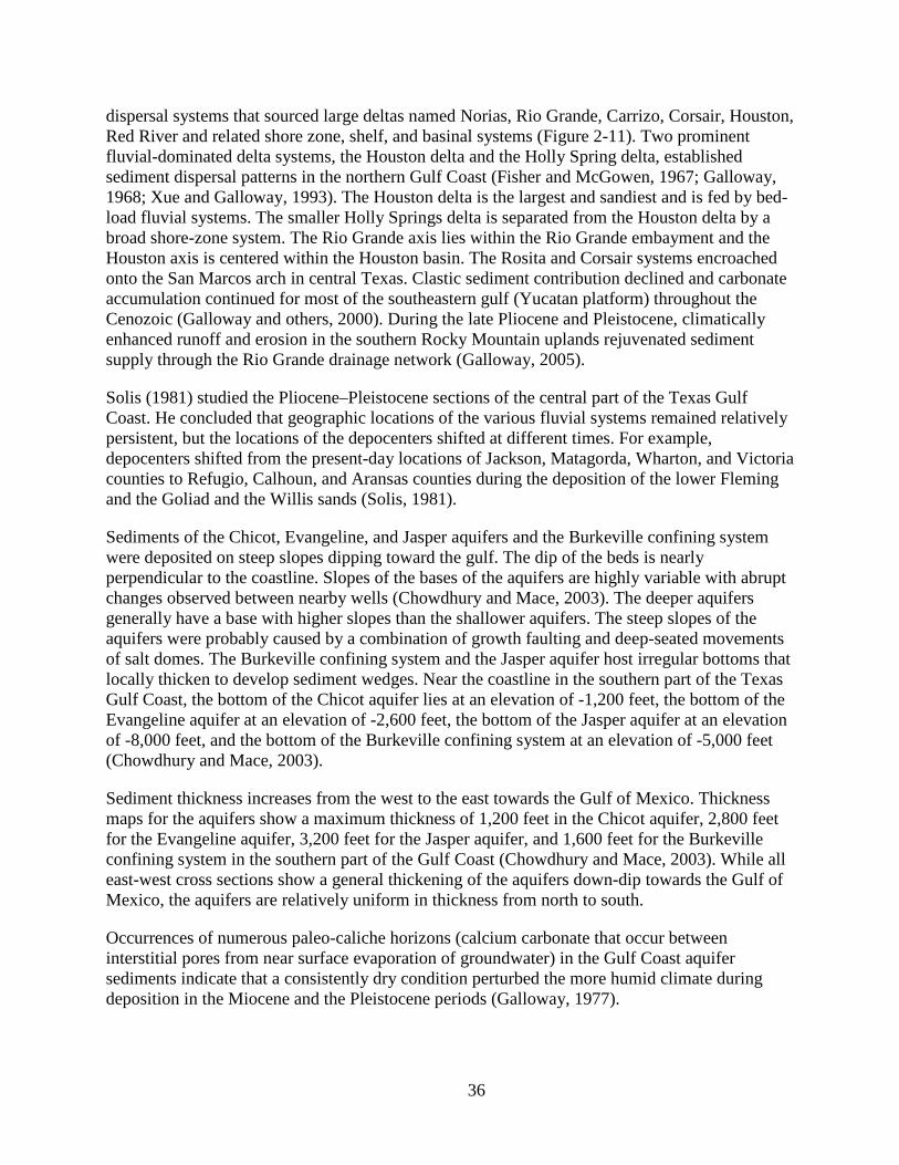
dispersal systems that sourced large deltas named Norias, Rio Grande, Carrizo, Corsair, Houston, Red River and related shore zone, shelf, and basinal systems (Figure 2-11). Two prominent fluvial-dominated delta systems, the Houston delta and the Holly Spring delta, established sediment dispersal patterns in the northern Gulf Coast (Fisher and McGowen, 1967; Galloway, 1968; Xue and Galloway, 1993). The Houston delta is the largest and sandiest and is fed by bed-load fluvial systems. The smaller Holly Springs delta is separated from the Houston delta by a broad shore-zone system. The Rio Grande axis lies within the Rio Grande embayment and the Houston axis is centered within the Houston basin. The Rosita and Corsair systems encroached onto the San Marcos arch in central Texas. Clastic sediment contribution declined and carbonate accumulation continued for most of the southeastern gulf (Yucatan platform) throughout the Cenozoic (Galloway and others, 2000). During the late Pliocene and Pleistocene, climatically enhanced runoff and erosion in the southern Rocky Mountain uplands rejuvenated sediment supply through the Rio Grande drainage network (Galloway, 2005).

Solis (1981) studied the Pliocene–Pleistocene sections of the central part of the Texas Gulf Coast. He concluded that geographic locations of the various fluvial systems remained relatively persistent, but the locations of the depocenters shifted at different times. For example, depocenters shifted from the present-day locations of Jackson, Matagorda, Wharton, and Victoria counties to Refugio, Calhoun, and Aransas counties during the deposition of the lower Fleming and the Goliad and the Willis sands (Solis, 1981).

Sediments of the Chicot, Evangeline, and Jasper aquifers and the Burkeville confining system were deposited on steep slopes dipping toward the gulf. The dip of the beds is nearly perpendicular to the coastline. Slopes of the bases of the aquifers are highly variable with abrupt changes observed between nearby wells (Chowdhury and Mace, 2003). The deeper aquifers generally have a base with higher slopes than the shallower aquifers. The steep slopes of the aquifers were probably caused by a combination of growth faulting and deep-seated movements of salt domes. The Burkeville confining system and the Jasper aquifer host irregular bottoms that locally thicken to develop sediment wedges. Near the coastline in the southern part of the Texas Gulf Coast, the bottom of the Chicot aquifer lies at an elevation of -1,200 feet, the bottom of the Evangeline aquifer at an elevation of -2,600 feet, the bottom of the Jasper aquifer at an elevation of -8,000 feet, and the bottom of the Burkeville confining system at an elevation of -5,000 feet (Chowdhury and Mace, 2003).

Sediment thickness increases from the west to the east towards the Gulf of Mexico. Thickness maps for the aquifers show a maximum thickness of 1,200 feet in the Chicot aquifer, 2,800 feet for the Evangeline aquifer, 3,200 feet for the Jasper aquifer, and 1,600 feet for the Burkeville confining system in the southern part of the Gulf Coast (Chowdhury and Mace, 2003). While all east-west cross sections show a general thickening of the aquifers down-dip towards the Gulf of Mexico, the aquifers are relatively uniform in thickness from north to south.

Occurrences of numerous paleo-caliche horizons (calcium carbonate that occur between interstitial pores from near surface evaporation of groundwater) in the Gulf Coast aquifer sediments indicate that a consistently dry condition perturbed the more humid climate during deposition in the Miocene and the Pleistocene periods (Galloway, 1977).

37

Stratigraphy In the Texas Gulf Coast, considerable heterogeneity of the sediments, discontinuity of the beds, and a general absence of index fossils and diagnostic electric log signatures in the subsurface often make correlation of the lithologic units difficult. Since 1903, at least seven stratigraphic classifications have been proposed (Kreitler and others, 1977). Guevera-Sanchez (1974) identified only the Beaumont and undifferentiated Lissie-Willis sands in the subsurface. Rose (1943a) classified the upper Miocene and Pliocene-Pleistocene sediments into seven zones based on permeability and sand percentage. The most permeable and heavily pumped Alta Loma Sand lies within zone 7 (Rose, 1943b). Wood and others (1963) considered the Beaumont Clay as a confining unit that extends from the land surface to the top of the Alta Loma Sand. Jorgensen (1975) classified Rose’s zones into the Chicot aquifer, with the Alta Loma Sand at its base, and defined the underlying units as the Evangeline aquifer.

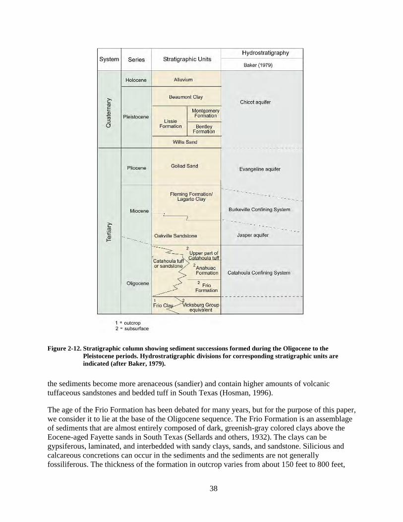
From oldest to youngest, he classified the Tertiary rocks into the Frio Formation, the Anahuac Formation, and the Catahoula Tuff or Sandstone (early Miocene); the Oakville Sandstone and the Fleming Formation (mid- to late-Miocene); the Goliad Sand (Pliocene); the Willis Sand, Bentley Formation, Montgomery Formation, and Beaumont Clay (Pleistocene); and alluvium (Holocene) (Baker, 1979) (Figure 2-12). The Catahoula Tuff or Sandstone, Goliad Sand, Willis Sand, and Beaumont Clay are often interchangeably referred to in the literature as formations (Sellards and others, 1932; Baker, 1979). Given the complexity of identifying the base of the Pleistocene from electric logs, several nomenclatures have been used to characterize these sediments. For example, Solis (1981) defined the base of the Pleistocene to be represented by the Lissie Formation. The undifferentiated Lissie Formation has also been considered equivalent in age to the Montgomery and the Bentley formations with the bottom of the latter being considered the base of the Pleistocene (Dutton and Richter, 1990). The Montgomery Formation is also occasionally included within the Beaumont Clay (Baker and Dale, 1961). In place of the Montgomery and the Bentley formations, the undifferentiated Lissie Formation of equivalent age occurs in the Lower Rio Grande Valley (Baker and Dale, 1961; Bureau of Economic Geology, 1976). The stratigraphic section of Baker (1979) is the basis for the summary information that follows.

Oligocene Series

Although some controversy exists in the literature, the Oligocene-aged sediments constitute the base of the Gulf Coast aquifer in Texas. The contact between the Oligocene-aged sediments and the underlying Eocene-aged sediments is mostly indistinguishable based solely on lithology. Paleontological differences associated with the Oligocene and Eocene Series are more commonly used to identify the difference between the two units. Throughout the entire extent of the Gulf Coast aquifer, most of the marine deposits in the lower part of the Oligocene belong to the Vicksburg Group or equivalent strata (Hosman, 1996). The Vicksburg Group is a regional confining unit that separates the Coastal Uplands aquifer system from the Coastal Lowlands aquifer system and consists primarily of marine clays and thin-bedded sandstones of the Eocene-aged Jackson Group and the Oligocene-aged Frio Clay, or Frio Formation, in the subsurface. Above this predominantly marine sequence that lies in the lower part of the Oligocene deposits,

38

Figure 2-12. Stratigraphic column showing sediment successions formed during the Oligocene to the Pleistocene periods. Hydrostratigraphic divisions for corresponding stratigraphic units are indicated (after Baker, 1979).

the sediments become more arenaceous (sandier) and contain higher amounts of volcanic tuffaceous sandstones and bedded tuff in South Texas (Hosman, 1996).

The age of the Frio Formation has been debated for many years, but for the purpose of this paper, we consider it to lie at the base of the Oligocene sequence. The Frio Formation is an assemblage of sediments that are almost entirely composed of dark, greenish-gray colored clays above the Eocene-aged Fayette sands in South Texas (Sellards and others, 1932). The clays can be gypsiferous, laminated, and interbedded with sandy clays, sands, and sandstone. Silicious and calcareous concretions can occur in the sediments and the sediments are not generally fossiliferous. The thickness of the formation in outcrop varies from about 150 feet to 800 feet,

39

whereas beneath the surface the thickness ranges from 250 feet to 600 feet (Sellards and others, 1932). The lack of sand and fossils in the sediments suggest that the adjoining land masses were low and near sea level during deposition and that the clays may have had a fresh-water origin.

The Catahoula Formation unconformably overlies the Frio Formation, which is unconformably overlain by the Oakville Formation (Figures 2-12, 2-13, and 12-14) (Baker, 1979). The basal contact of the Catahoula Formation is delineated by the presence of coarse-grained sand and conglomerate and the underlying Jackson Sandstone in East Texas or the Frio Formation in South Texas. Specific information on the stratigraphy of the Catahoula Formation members can be found in Sellards and others (1932). The Catahoula Formation is composed of non-marine sands and clays and volcano-clastic deposits interbedded with fluviatile sediments. Surface hydrology dictated the degree of coarseness of the sediments, with larger sand grains deposited in the larger East Texas rivers and the finer sediments deposited in the smaller, lower-energy rivers of South Texas. All types and sizes of volcanic deposits are found in the Catahoula Formation, which suggests multiple source locations. The Catahoula Formation consists of approximately 60 percent volcanic material and 30 percent sandstone. The average thickness of the Catahoula Formation in the Texas Gulf Coast ranges from 200 to 600 feet in East Texas, thins to about 150 to 200 feet in Central Texas, and then thickens to about 800 to 1000 feet in South Texas. Downdip, the Catahoula Formation rapidly thickens and, at about 2,000 feet below sea level, a gulfward thickening accretionary wedge of fossiliferous marine clay appears in the upper section. This clay, called the Anahuac Formation,is overlain by the upper part of the Catahoula Formation and overlies the Frio Formation (Hosman, 1996).

Miocene Series

The Miocene sediments comprise the Jasper aquifer and the Burkeville confining system (Baker, 1979), with the Jasper being the deepest confined water-bearing unit in the Gulf Coast aquifer system in Texas (Figures 2-12, 2-13, and 12-14). The depositional environment during the Miocene in the Gulf of Mexico Coastal Plain was essentially regressive. Intermittent sea-level reversals at various locations along the Gulf Coast produced minor transgressive cycles within the overall depositional pattern, resulting in fossiliferous marine strata ideal for correlations (Hosman, 1996). Typically, the sediments are complexly interbedded sands, silts, and clays with intermixed volcano-clastic and tuffaceous material.

The Oakville Sandstone and the Fleming Formation are composed almost entirely of terrigenous clastic sediments containing interbedded sand and clays (Baker, 1979). The Oakville Sandstone unconformably overlies the Catahoula Formation and is unconformably overlain by the Lagarto Clay of the Fleming Formation. The Oakville Sandstone generally extends in outcrop from the Brazos River basin to the Rio Grande, with the exception of areas south of Duvall County, where it is overlain by Pliocene deposits. North of the Brazos River, it is lithologically indistinguishable from the Fleming Formation but can be correlated by using vertebrate fossils (Sellards and others, 1954). The thickness of the Oakville Sandstone increases southward and gulfward to more than 500 feet in some areas (Sellards and others, 1954). Unique marine fossils found in the sediments of the Oakville Formation are used to distinguish it from adjacent geologic units.

The Fleming Formation extends throughout the Gulf Coast aquifer system in Texas and eastern Louisiana. In South Texas, the Fleming Formation is primarily composed of clays, with the

40

(a)

Figure 2-13a. Cross-section showing thicknesses of the aquifers along strike (north-south) in the central and southern parts of the Gulf Coast. Cross-section lines are shown in inset map (from Solis, 1981). Formations thicken downdip but remain relatively uniform in thickness along strike. Note sediment thickness varies considerably across faults, suggesting fault involvement during deposition. Depositional environment for each sediment facies and fresh water contact at depth are indicated.

percentage of sand increasing eastward towards the Sabine River. The clay beds can be many different colors and the strata can contain a thin layer of chalky sandstone as well as finely crossbedded sands in some locations (Hosman, 1996). Although the Fleming Formation is lithologically similar to the Oakville Sandstone, it is easily differentiated from the Oakville Sandstone in some places by its greater percentage of clay (Baker, 1979). While it is only about 200 feet thick in the outcrop, the Fleming Formation is thousands of feet thick downdip along the coast (Hosman, 1996). The Fleming Formation contains the Burkeville confining system and may include portions of both the Jasper aquifer at depth and the Evangeline aquifer towards up-dip areas. The Fleming Formation defines the most up-dip extent of the Miocene-aged water-bearing units in the Gulf Coast aquifer system in Texas.

41

(b)

Figure 2-13b. Cross-section showing thicknesses of the aquifers down-dip (east-west) in the central and southern parts of the Gulf Coast (from Solis, 1981).

Pliocene Series

The Pliocene-aged sediments are for the most part very similar to the Miocene-aged sediments, but may differ somewhat lithologically (Hosman, 1996). Pliocene-aged sediments can be more arenaceous and interbedded than those of the Miocene-aged sediments; the clays are less calcareous and the sands more lignitic. However, considering these differences, the Pliocene sediments are difficult to distinguish from the underlying Miocene sediments. Additionally, distinguishing between the Pliocene-aged sediments and the overlying Pleistocene-aged sediments is difficult and has resulted in similar degrees of controversy amongst geologists.

The Goliad Formation overlies the Fleming Formation and consists of coarse-grained sediments, including cobbles, clay balls, and wood fragments at the base of the formation (Hosman, 1996). The upper part of the Goliad Formation consists of finer-grained sands that are cemented with calcium carbonate called caliche (Hosman, 1996). Caliche is a surface deposit formed in semi-arid climates by the evaporation of surface waters carrying calcium bicarbonate in solution,

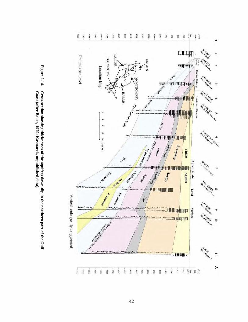
42

Figure 2-14. Cross-section show

ing thicknesses of the aquifers down-dip in the northern part of the G

ulf C

oast (after Baker, 1979; Kasm

arek, unpublished data).

43

leaving the calcium carbonate precipitated in the pore spaces within the sand and gravel beds (Sellards and others, 1954). The irregular bedding, presence of gravel, and presence of some caliche in the Goliad Formation suggest a high-energy riverine depositional environment early in the Pliocene with shorter duration of semi-aridity throughout the Pliocene. The sands of the Goliad Formation are interbedded with grayish clays that are locally marly (Hosman, 1996). The sands in the Goliad Formation are typically whitish gray or pinkish grey, but in areas of increased amounts of chert it can have a salt-and-pepper appearance (Sellards and others, 1932). The Goliad Formation is entirely within the Evangeline aquifer and the upper boundary of the Evangeline aquifer probably follows closely with the top of the Goliad Formation where present (Baker, 1979).

Pleistocene and Holocene Series

The depositional environment of the Pleistocene-aged sediments is consistent with the erosional and sedimentary cycles associated with periods of glaciation and coincident sea-level variations. Coastal terrace deposits and a fining upward sequence are typical of glacial cycling (Hosman, 1996). The Lissie Formation and Beaumont Clay are the two dominant subdivisions of the Pleistocene system. The Alta Loma Sand and the Willis Formation are locally extensive, occur over a small geographic area, and represent part of the Pleistocene system. The Holocene system consists of river alluvium and coastal deposits. The Chicot aquifer is contained entirely within the Pleistocene- and Holocene-aged sediments.

The Alta Loma and Willis sands are complexly faulted. These fluvial-deltaic sediments have been identified in the subsurface in Harris, Galveston, Chambers, and Brazoria counties (Kreitler and others, 1977). Evaluation of electric logs shows a coarsening-upward sequence, commonly indicative of delta-front facies (Kreitler and others, 1977). The Alta Loma Sand doubles in thickness from 200 feet in Harris County to 400 feet in Brazoria and Galveston counties due to fault-induced displacement of the sand.

The Willis Sand was used to describe a sequence of unfossiliferous sand and gravelly sand beds overlying the Fleming Formation in Southeast Texas (Doering, 1935; Solis, 1981). Plummer (1933) described these sediments as reddish, coarse, and gravelly sands with subordinate clays that grade into the Goliad Formation in the southwest of the Gulf Coast (Doering, 1935). In the Rio Grande region, the Willis Sand has not been identified (Weeks, 1937).

The Lissie Formation is unconformably contained between the Goliad Sand and the overlying Beaumont Clay. The Lissie Formation crops out in a band parallel to the coast and is about 30 miles wide from the Sabine River to the Rio Grande. The sediments of the Lissie Formation in the outcrop are partly continental deposits laid down on flood plains and partly as delta sands, silts, and mud at the mouth of rivers (Sellards and others, 1932). The Lissie Formation hosts flatter, gently undulating topography, and has much lower-dipping beds than the Goliad Sand. Lissie Formation sediments consist of reddish, orange, and gray fine- to coarse-grained, cross-bedded sands. Over most of Brooks and Hidalgo counties to the south, the Lissie Formation is either eroded or covered by sand dunes. Thin beds of the Lissie Formation crop out over a small area in southern Hidalgo and northern Willacy counties. The sands in the Lissie Formation are fine-grained and the formation contains relatively less conglomerates than the underlying Goliad Sand. Caliche beds often mark the base of the Lissie Formation (Price, 1934).

44

The Beaumont Clay is contained between the underlying Lissie Formation and overlying Holocene-aged stream deposits and wind blown sands. It outcrops from the Sabine River in the east to Kleberg County in the south. The Beaumont Clay is made up of poorly bedded, marly clay and is interbedded with lenses of sand in the north (Figure 2-15) (Sellards and others, 1932). In South Texas, the Beaumont Clay forms a thin mantle that extends eastward from Rio Grande City in Starr County to Hidalgo County (Weeks, 1937). In Starr and western Hidalgo counties, the Beaumont Clay is sandy but is composed of reddish-brown clay and some sand beds farther east (Weeks, 1937). The Beaumont Clay is contemporaneous with the Beaumont Sand, which can be generally continuous on a local scale. The Beaumont sediments were deposited largely by rivers in the form of natural levees and deltas that coalesced as river mouths shifted along the coast and, to a lesser extent, by marine and lagoonal water in the bays and embayments between stream ridges and delta banks (Sellards and others, 1932).

The Holocene-aged alluvial systems in the Texas Gulf Coast are local in scale and typically are included within the Chicot aquifer. The Brazos, Trinity, Nueces, and Rio Grande alluvial basins consist of terrace gravels, buried sand deposits, and point bar deposits with grain sizes ranging from clay to gravel. The flat-lying floodplain deposits typically consist of sand and gravel in the lower part and silt and clay in the upper part. This surficial system exhibits the largest outcrop area of all the units in the Texas Gulf Coast and provides a direct hydraulic connection in some cases between the surface water and groundwater systems.

Figure 2-15. Photograph of a core of the Beaumont Clay at a depth of about 30 feet from a well near Houston. Whitish areas are carbonates, darker areas are organic matter, and pinkish (gray) areas are clay. Note tightness of the clay that retards any significant infiltration of recharge.

45

Conclusions 1. The Gulf of Mexico Basin was formed by downfaulting and downwarping of the

Paleozoic basement rocks during the breakup of the Paleozoic megacontinent Pangaea and opening of the North Atlantic Ocean in the Late Triassic. Sediments of the Gulf Coast aquifer in Texas were deposited in the costal plains of the Gulf of Mexico Basin during the Tertiary and the Quaternary periods.

2. Structures in the Gulf Coast aquifer in Texas include the Balcones fault zone, Texas-Mexia fault zone, San Marcos arch, Sabine arch, Rio Grande embayment, numerous growth faults, and salt domes. These structural features controlled the accumulation and distribution of sediments, as supported by the observation that bedding commonly thins towards and over the arches and thickens in the embayments. Most of the growth faults and salt domes are mainly caused by gravity acting on thick sedimentary sections deposited on abnormally pressured shale or salt that sole out above the basement to produce salt-flow structures and growth faults. Salt domes and growth faults provide structural and stratigraphic traps for oil and gas fields in the prolific hydrocarbon-bearing Gulf of Mexico basin.

3. Sediments of the Gulf Coast aquifer in Texas were deposited under fluvial-deltaic to shallow-marine environments. Repeated sea-level changes and natural basin subsidence produced discontinuous beds of sand, silt, clay, and gravel. Six major sediment dispersal systems that sourced large deltas distributed sediments eroding from the Laramide Uplift along the central and southern Rockies and the Sierra Madre Oriental in northern Mexico. Geographic locations of the various fluvial-dominated systems remained relatively persistent, but the locations of the depocenters where thickest sediment accumulations occurred shifted at different times.

4. Rapid sediment loading in fluvial deltas caused overpressure zones to develop in the subsurface. Overpressure developed as connate water trapped during deposition was unable to escape during rapid burial of the sediments, giving rise to high fluid pressure.

5. The stratigraphic framework of the Gulf Coast aquifer sediments is complex and controversial, with disagreement over which units are equivalent in age and how they correlate with each other in the outcrop or the subsurface. The considerable heterogeneity of the sediments, discontinuity of the beds over short distances, a general absence of index fossils or marker beds, and an absence of diagnostic electric log signatures in the subsurface often make correlation of the lithologic units difficult.

6. The Gulf Coast aquifer in Texas consists of five hydrostratigraphic units, from oldest to youngest: the Catahoula Confining System, the Jasper aquifer, the Burkeville confining system, the Evangeline aquifer, and the Chicot aquifer. Although several stratigraphic classifications have been proposed, this classification scheme, based on detailed faunal information, lithology and electric log signatures, and hydraulic characteristics of the sediments can be successfully used for facies correlations over most of the Texas Gulf Coast. Therefore, this classification is widely accepted by the geologic community.

46

References Aronow S. and Barnes. V. E., 1968, Geologic atlas of Texas, Houston Sheet, Paul Weaver

Memorial Edition.

Aronow S. and Barnes. V. E., 1975, Geologic atlas of Texas, Corpus Christi Sheet, Alva Christine Ellisor Memorial Edition.

Aronow, S., Brown, T. E., Brewton, J. L., Eargle, D. H. and Barnes, V. E., 1975, Geologic atlas of Texas, Beeville-Bay City Sheet, Alexander Deussen Memorial Edition.

Baker, R. C., and Dale, O. C., 1961, Groundwater resources of the Lower Rio Grande Valley area, Texas: Texas Board of Water Engineers, Bulletin 6014, 81 p.

Baker, E. T., Jr., 1979, Stratigraphic and hydrogeologic framework of part of the coastal plain of Texas: Texas Department of Water Resources Report 236, 43 p.

Bornhauser, M., 1958, Gulf Coast tectonics: American Association of Petroleum Geologists Bulletin, v. 42, p. 339–370.

Brewton, J. L., Owen, F., Aronow , S., and Barnes, V. E., 1976a, Geologic atlas of Texas, McAllen-Brownsville Sheet, Arthur Carleton Trowbridge Memorial Edition.

Brewton, J. L., Owens, F., Aronow, S., and Barnes, V. E., 1976b, Geologic atlas of Texas, Laredo Sheet, Julia Gardner Memorial Edition.

Bruce, C. H., 1973, Pressured shale and related sedimentary deformation—Mechanism for development of regional contemporaneous faults: American Association of Petroleum Geologists Bulletin, v. 57, p. 878–886.

Bryant, W. R., Lugo, J., Cordova, C., and Salvador, A., 1991, Physiography and bathymetry, in Salvador, A., editor, The Gulf of Mexico Basin: Boulder, Colorado, Geological Society of America, The Geology of North America, v. J., p. 13–30.

Bureau of Economic Geology, 1976, Geologic atlas of Texas, McAllen-Brownsville sheet: The University of Texas at Austin, Bureau of Economic Geology.

Byerly, G. R., 1991, Igneous activity, in Salvador, A., editor, The Gulf of Mexico Basin: Boulder, Colorado, Geological Society of America, The Geology of North America, v. J., p. 91–108.

Chowdhury, A. H., Bogichi, R. and Hopkins, J., this volume, Hydrochemistry, salinity distribution, and trace constituents—Implications for salinity sources, geochemical evolution, and flow system characterization: Proceedings of the Gulf Coast Aquifer Conference, Corpus Christi, Texas Water Development Board Report 365, p 81–128.

Chowdhury, A. H., and Mace, R. E., 2003, A groundwater availability model for the Gulf Coast aquifer in the Lower Rio Grande Valley, Texas—Numerical simulations through 2050: Texas Water Development Board, unpublished report, 171 p.

Cloos, E., 1962, Experimental analysis of Gulf Coast fracture patterns: American Association of Petroleum Geologists Bulletin, v. 52, p. 420–444.

Doering, J., 1935, Post-Fleming surface formations of coastal Southeast Texas and South Louisiana: Bulletin American Association of Petroleum Geologists, v. 19, p. 651–688.

47

Dutton, A. R. and Richter, B. C., 1990, Regional hydrogeology of the gulf coast aquifer in Matagorda and Wharton counties, Texas – Development of a numerical flow model to estimate the impact of water management strategies: Report prepared for the Lower Colorado River Authority under contract (88-89) 0910, Bureau of Economic Geology, University of Texas at Austin, 118 p.

Ewing, T. E., 1991, Structural framework, in Salvador, A., editor, The Gulf of Mexico Basin: Booulder, Colorado, Geological Society of America, The Geology of North America, v. J., p. 31–52.

Fisher, W. L., and McGowen, J. H., 1967, Depositional systems in the Wilcox Group of Texas and their relationship to the occurrence of oil and gas: Gulf Coast Association of Geological Societies Transactions, v. 17, p. 105–125.

Gabrysch, R. K., 1984, Case history no. 9.12. The Houston-Galveston region, Texas, USA, in Poland, J. F., editor, Guidebook to studies of land subsidence due to groundwater withdrawal: UNESCO Studies and Reports in Hydrology 20, p. 253–262.

Galloway, W. E., 1968, Depositional systems of the Lower Wilcox Group, North-Central Gulf Coast Basin: Gulf Coast Association of Geological Societies Transactions, v. 18, p. 275–289.

Galloway, W. E., 1977, Catahoula Formation of the Texas Coastal Plain, depositional systems, composition, structural development, groundwater flow, history and uranium distribution: The University of Texas at Austin, Bureau of Economic Geology, Report of Investigation no. 87, 59 p.

Galloway, W. E., 1989, Genetic sequences in basin analysis II—Application to northwest Gulf of Mexico Cenozoic basin: Bulletin American Association of Petroleum Geologists, v. 73, p. 143–154.

Galloway, W. E., 2005, Gulf of Mexico Basin depositional record of Cenozoic North American drainage basin evolution: International Association of Sedimentologists Special Publication 35, p. 409–423.

Galloway, W. E., Ganey-Curry, P. E., Li, X., and Buffler, R., 2000, Cenozoic depositional history of the Gulf of Mexico Basin: American Association of Petroleum Geologists Bulletin, v. 84, p. 1743–1774.

Grubb, H. F., 1998, Summary of hydrology of the regional aquifer systems, Gulf Coastal plain, South-Central United States—Regional aquifer system analysis—Gulf Coastal Plain: U.S. Geological Survey Professional paper 1416-A, p. 61 p.

Guevara-Sanchez, E. H., 1974, Pleistocene facies in the subsurface of the southeast Texas Coastal Plain: The University of Texas at Austin, unpublished Ph.D. dissertation, 133 p.

Halbouty, M. T., and Halbouty, J. J., 1982, Relationships between East Texas Field region and the Sabine uplift in Texas: American Association of Petroleum Geologists Bulletin, v. 66, p. 1042–1054.

Hamlin, S., this volume, Salt domes in the Gulf Coast aquifer: Texas Water Development Board Report 365, p. 217–230.

48

Hosman, R. L., 1996, Regional stratigraphy and subsurface geology of Cenozoic deposits, Gulf Coastal Plain, South-Central United States—Regional aquifer system analysis—Gulf Coastal Plain: U.S. Geological Survey Professional Paper 1416-G, 35 p.

Hosman, R. L. and Weiss, J. S., 1991, Geohydrologic units of the Mississippi Embayment and Texas Coastal Uplands Aquifer Systems, South-Central United States—Regional aquifer system analysis—Gulf Coastal Plain: U.S. Geological Survey Professional Paper 1416-B, 19 p.

Jackson, M. P. A., and Galloway, W. E., 1984, Structural and depositional styles of Gulf Coast Tertiary continental margins—Applications to hydrocarbon exploration: Continuing Education Course Notes Number 25, American Association of Petroleum Geologists, 225 p.

Jones, P. H., 1969, Hydrology of Neogene deposits in the northern Gulf of Mexico basin: Louisiana State University, Louisiana Water Resources Research Institute Bulletin GT-2, 105 p.

Jorgensen, D. G., 1975, Analog-model studies of groundwater hydrology in the Houston district, Texas: Texas Water Development Board Report 190, 84 p.

Kasmarek, M. C., and Robinson, J. L., 2004, Hydrogeology and simulation of groundwater flow and land-surface subsidence in the northern part of the Gulf Coast aquifer system: U.S. Geological Survey, Scientific Investigations Report 2004-5102, 111 p.

Kreitler, C. W., Guevera, E., Granata, G., and McKalips, D., 1977, Hydrogeology of the Gulf Coast aquifers, Houston-Galveston area, Texas: Transactions—Gulf Coast Association of Geological Societies, v. XXVII, p. 72–89.

Leach, W. G., 1994, Distribution of hydrocarbons in abnormal pressure in South Louisiana, USA, in Fertl, W. H., Chapman, R. E., and Holtz, R. F., editors, Studies in Abnormal Pressures: Elsevier.

Leach, W. G., and Fertl, W. H., 1990, The relationship of formation pressure and temperature to lithology and hydrocarbon distribution in Tertiary sandstones: Tranactions of the International Well Logging Symposium, section E, Beijing, China.

McCoy, T. W., 1990, Evaluation of groundwater resources in the Lower Rio Grande Valley, Texas: Texas Water Development Report 316, 47 p.

Morton, R. A., Han, J. H., and Posey, J. S., 1983, Variations in chemical composition of Tertiary formation waters, Texas Gulf Coast, in Morton, R. A., and others, editors, Consolidation of geologic studies of geopressured geothermal resources in Texas, 1982 Annual Report: The University of Texas at Austin, Bureau of Economic Geology, report prepared for the U.S. Department of Energy under contract no. DE-AC08-79ET27111, p. 63–135.

Mukherji, T., Dutta, N., Prasad, M., and Dvorkin, J., 2002, Seismic detection and estimation of overpressures, Part I: the Rock Physics Basics, Canadian Society of Exploration Geophysicists Recorder, p. 36–57.

Murray, G. E., 1961, Geology of the Atlantic and Gulf Coastal Province of North America: New York, Harper and Brothers, 692 p.

49

Nelson, T. H., 1991, Salt tectonics and listric-normal faulting, in Salvador, A., editor, The Gulf of Mexico basin: Geological Society of America, The Geology of North America, v. J., p. 73–89.

Plummer, F. B., 1933, Cenozoic Systems in Texas: Geology of Texas, vol. 1, Stratigraphy, University of Texas Bulletin 3232, p. 519–818.

Price, W. A., 1934, Lissie Formation and Beaumont Clay in South Texas: Bulletin of the American Association of Petroleum Geologists, v.18, no. 7, p.948–959.

Proctor, C. V., Brown, T. E., Waechter, N. B., Aronow, S., and Barnes, V. E., 1974, Geologic atlas of Texas, Seguin Sheet, Donald Clinton Barton Memorial Edition.

Quarles, M., 1952, Salt-ridge hypothesis of Texas Gulf Coast type of faulting: American Association of Petroleum Geologists Bulletin, v. 37, p. 489–508.

Rose, N. A., 1943a, Groundwater and relationship of geology to its occurrence in Houston district, Texas: Bulletin of the American Association of Petroleum Geologists, v. 27, p. 1081–1101.

Rose, N. A., 1943b, Progress report on the groundwater resources of the Texas City area, Texas: U.S. Geological Survey Open-file report, 45 p.

Salvador, A., 1991, Introduction, in Salvador, A., editor, The Gulf of Mexico Basin: Geological Society of America, The Geology of North America, v. J., p. 1–12.

Sellards, E. H., Adkins, W. S., and Plummer, F. B., 1932, The Geology of Texas, Volume I, Stratigraphy: The University of Texas at Austin, Bureau of Economic Geology, 1007 p.

Shah, S. D., and Lanning-Rush, J., 2005, Principal faults in the Houston, Texas, Metropolitan Area: U.S. Geological Survey Scientific Investigations Map 2874, 4 p.

Shelby, C. A., Pieper, M. K., Aronow, S., and Barnes, V. E., 1968, Geologic atlas of Texas, Beaumont Sheet, Harold Norman Fisk Memorial Edition.

Solis, R. F., 1981, Upper Tertiary and Quaternary depositional systems, central Coastal Plain, Texas—Regional geology of the coastal aquifer and potential liquid-waste repositories: The University of Texas at Austin, Bureau of Economic Geology Report of Investigations 108, 89 p.

Spearing, D., 1991, Roadside geology of Texas: Mountain Press Publishing Company, Missoula, Montana, 418 p.

Strom, E. W., Houston, N. A., and Garcia, C. A., 2003a, Selected hydrologic data sets for the Chicot aquifer: U.S. Geological Survey, Open File Report.03-297, 1 CD-ROM.

Strom, E. W., Houston, N. A., and Garcia, C. A., 2003b, Selected hydrologic data sets for the Evangeline aquifer: U.S. Geological Survey, Open File Report 03-298, 1 CD-ROM.

Strom, E. W., Houston, N. A., and Garcia, C. A., 2003c, Selected hydrologic data sets for the Jasper aquifer: U. S. Geological Survey, Open File Report 03-299, 1 CD-ROM.

Verbeek, E. R., Ratzlaff, K. W., and Clanton, U. S., 1979, Faults in parts of north-central and western Houston metropolitan area, Texas: U.S. Geological Survey Miscellaneous Field Studies Map MF-1136, 1 sheet.

50

Vogler, H. A., and Robinson, B. A., 1987, Exploration for deep geopressured gas, Corsair trend, offshore Texas: American Association of Petroleum Geologists Bulletin, v. 71, p. 777–787.

Weeks, A. W., 1937, Miocene, Pliocene and Pleistocene formations in Rio Grande region, Starr and Hidalgo counties, Texas: Bulletin of the American Association of Petroleum Geologists, v. 21, no. 4, p. 491–499.

Williamson, A. K. and Grubb, H. F., 2001, Groundwater flow in the Gulf Coast aquifer systems, Regional aquifer system analysis—Gulf Coastal Plain, U.S. Geological Survey Professional Paper 1416-F, 173 p.

Wood, L. A., Gabrysch, R. K., and Marvin, R., 1963, Reconnaissance investigation of the groundwater resources of the Gulf Coast region, Texas: Texas Water Commission, Bulletin 6305, 114 p.

Xue, L., and Galloway, W. E., 1993, Sequence stratigraphy and depositional framework of the Paleocene Lower Wilcox strata, Northwest Gulf of Mexico Basin: Gulf Coast Association of Geological Societies Transactions v. 43, p. 453–464.

51

Chapter 3

The Yegua-Jackson Aquifer Richard D. Preston, P.G.1

Introduction The occurrence of usable quality water is very erratic through most of the extent of the Yegua-Jackson aquifer. However, over much of this area, few other economically viable sources of groundwater are available. In some of the area, water-bearing sediments of the Carrizo-Wilcox, Queen City, and Sparta aquifers dip beneath the Yegua-Jackson aquifer, but the expense and depth of required wells and/or possible treatment of poorer water quality complicates possible use. The aquifer is located north of the Gulf Coast aquifer and south of the Carrizo-Wilcox, Queen City, and Sparta aquifers. Total water use from the aquifer is relatively high and the Yegua-Jackson aquifer is currently providing water for most purposes. Historically, the Jackson Group and the Yegua Formation were considered under the umbrella term “other aquifer” by the U.S. Geological Survey (USGS) and the Texas Water Development Board (TWDB) (Ashworth and Hopkins, 1995). The aquifer was delineated in the preparation of the TWDB’s 2002 Water Plan as a minor aquifer to be called the Yegua-Jackson aquifer. The delineation was deemed necessary because of the large number of wells in the TWDB files and the relatively large use of water from this source.

Location and Extent The Yegua-Jackson aquifer extends in a narrow band (15 to 40 miles wide) from the Rio Grande and Mexico across the state to the Sabine River and Louisiana. This band is from 70 to 120 miles inland and of generally parallels the Gulf of Mexico coast. The extent of the Yegua-Jackson aquifer is shown on Figure 3-1. The aquifer as currently delineated extends over parts of 35 counties (Texas Water Development Board, 2002).

Climate and Geography The climate of the area of Texas covered by the Yegua-Jackson aquifer is sub-tropical and is humid in the eastern and central part, subhumid in the western part, and steppe along the Rio Grande. Rainfall varies greatly across the extent of the aquifer, from an average of over 50 inches per year in Sabine County on the Louisiana border in East Texas to about 20 inches per

1 Private consultant, formerly with Texas Water Development Board

52

Figure 3-1. Extent of the Yegua-Jackson aquifer in Texas.

year in Starr County on the Mexican border in the Lower Rio Grande Valley in far South Texas. Gross lake-surface evaporation ranges from about 31 inches per year on the Sabine River in East Texas to about 51 inches per year on the Rio Grande in West Texas (Larkin and Bomar, 1983). From east to west, the aquifer is crossed by the Sabine, Trinity, Angelina, Brazos, Colorado, Guadalupe, San Antonio, and Nueces rivers and the Rio Grande. The area is part of the upper coastal plain of the Gulf of Mexico, and local relief is generally a few tens of feet, with the land surface sloping gently to the south and east toward the coast (Larkin and Bomar, 1983). Some of the rare, isolated, indurated sandstones within the section hold up a few low, strike-oriented hills and questas with slightly greater relief.

53

Previous Investigations Little previous detailed work has been completed on the Yegua-Jackson aquifer in Texas. Despite the fact that the Yegua Formation and the Jackson Group are represented in USGS and TWDB by more than 1,600 wells in TWDB and USGS databases, these aquifers were not recognized as a named aquifer until the 2002 state water plan. Since the surface areas of the two aquifers are contiguous and sometimes overlap, they were delineated as one aquifer, the Yegua-Jackson.

Significant studies of oil and gas, lignite, and uranium occurrence and mining from the Yegua Formation and Jackson Group rocks are included in the References section of this report and are the source of much of the geologic information available. TWDB and USGS reports have been completed for several of the 35 counties that are at least partially underlain by this aquifer. Again, these have been listed in the References section.

The database of the TWDB contains records of more than 1,600 wells completed at least partially in the rocks of the Yegua-Jackson aquifer, along with many chemical analyses, water levels, driller’s logs, and other information. This data is available in the TWDB offices or on the TWDB web site (www.twdb.state.tx.us).

Hydrogeology The Yegua Formation (part of the upper Claiborne Group) and the Jackson Group (made up of the Whitsett, Manning, Wellborn, and Caddell formations) are part of the upper Eocene–Pleistocene series of cyclic progradational sedimentation (Figure 3-2). These cycles were controlled by land subsidence along the coast as a part of the Gulf Coast geosyncline and coastline migration in response to periodic glaciation, which reduced the area of the gulf and oceans. They consist of complexly interbedded sands, silts, and clays that are fluvial and deltaic

Figure 3-2. A simplified stratigraphic column of the Upper Claiborne and Jackson groups (modified from Jackson and Garner, 1982).

54

in origin (Galloway and others, 1979). A few thin clays and shales are probably of marine origin, representing minor transgressive pulses. These sequences thicken greatly into the subsurface toward to coast and into the gulf geosyncline (Hamilton, 1994). The source of much of these sediments is volcanic. In some areas, significant amounts of lignite occur within both the Yegua Formation and the Jackson Group. They are thought to have been deposited in swampy areas along the rivers and along the coastal flatlands (Jackson and Garner, 1982). The rocks of the Cook Mountain Formation, which underlie the Yegua Formation, are mostly marine (Jackson and Garner, 1982). The sediments of the Catahoula Formation, which overlie the Jackson Group, are thought to be fluvial. The Catahoula Formation is overlain by sediments that represent the start of a major transgressive cycle (Galloway and others, 1979).

Groundwater occurs within the sand units of the aquifer, with the more significant amounts of water occurring within areas of more extensive fluvial channel sands and thick deltaic sands. Thus many of the more productive existing wells are found within the trends of the ancestors of such rivers as the Trinity, Colorado, and Brazos (Jackson and Garner, 1982). Usable quality groundwater is generally limited to sands in the outcrop or slightly downdip.

Strike within these sediments generally parallels the present Texas gulf coast. Dip varies from about 20 to 360 feet per mile, steepening toward the coast and into the gulf basin. Within the area delineated as the Yegua-Jackson aquifer, the steeper dips are often associated with salt domes that partially penetrate the underlying sediments (Jackson and Garner, 1982).

The main source of recharge to the Yegua-Jackson aquifer is from rainfall and runoff on the outcrop of the sandy, more permeable part of the aquifer. Significant additional recharge is derived from the rivers and their tributaries crossing the outcrop area. Within the floodplains of some of the rivers, recent alluvial deposits overlie some of the permeable sands and provide another source of additional recharge. Remnants of older Tertiary alluvial deposits of sand and gravel occur erratically at higher elevations and also provide recharge to the Yegua-Jackson aquifer (Jackson and Garner, 1982). As indicated by springs and seeps in parts of the lower topographic areas, a significant part of the water recharged to the aquifer is rejected back to the streams as spring and return flow. Additional discharge is through wells.

Known well yields range from a few gallons per minute (gpm) to over 300 gpm. Properly located, designed, and constructed wells sited in the most productive areas might produce up to 500 to 600 gpm. Figure 3-3 shows long-term water level changes in several wells located in different parts of the aquifer. Numerous TWDB reports discussing the occurrence and chemical quality of groundwater for individual counties contain information on the Yegua-Jackson aquifer. Well data for over 1,600 wells is available in the data files of the TWDB.

Water Quality The chemical quality of groundwater produced from wells and springs completed in the rocks of the Yegua-Jackson aquifer is extremely erratic (Jackson and Garner, 1982). It is affected by the composition of the mostly volcanic sediments that make up the aquifer and by the lignite and radioactive compounds that have been deposited and/or emplaced within these rocks. This has led to the occurrence of relatively high concentrations of chloride and sulfate even within quite

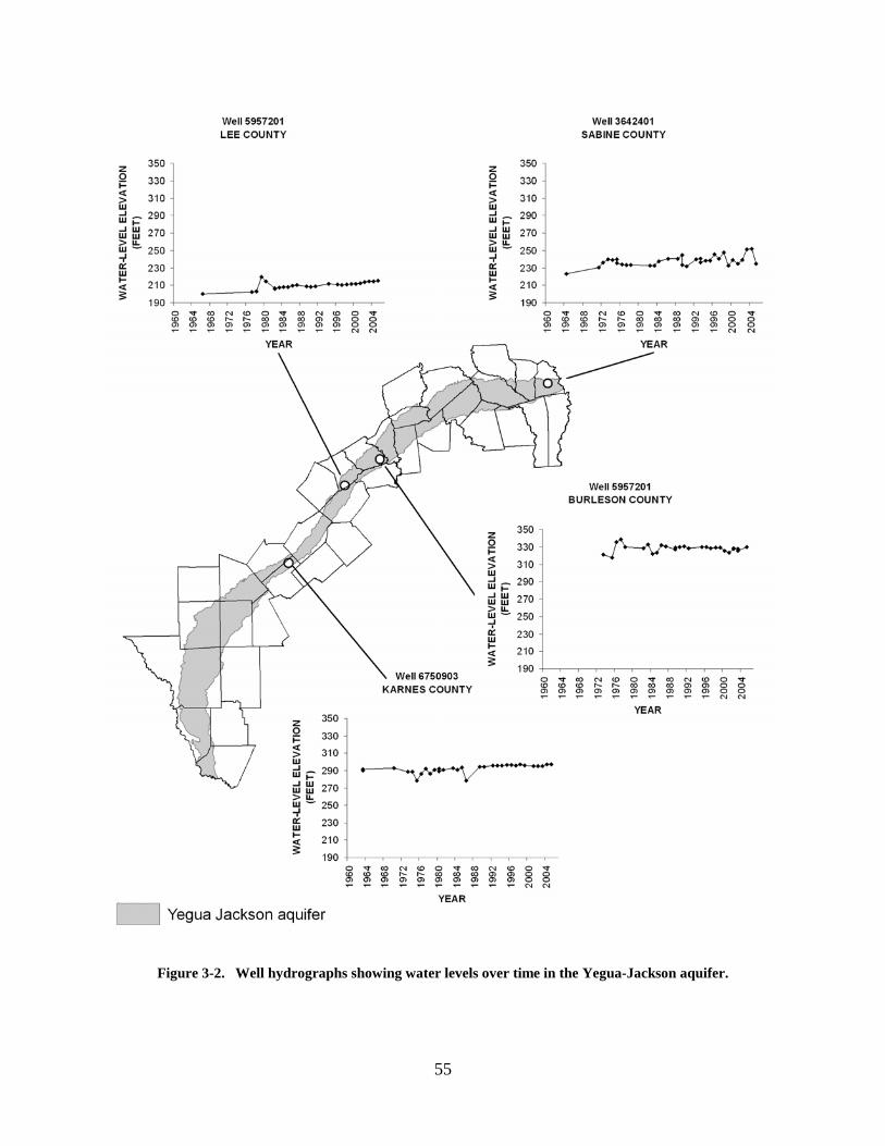
55

Figure 3-2. Well hydrographs showing water levels over time in the Yegua-Jackson aquifer.

56

shallow sands near these minerals. Numerous instances of high radioactivity have been found in water produced in and near the areas of uranium occurrence and mining.

Where the thicker, more extensive sands of fluvial and deltaic origin occur on the outcrop and slightly down dip, significant amounts of fresh-to slightly-saline water are available from the Yegua-Jackson aquifer. Much of this water meets the requirements for most uses, including public supply. In some cases, even when limits are exceeded, no other economically viable source is available. As reported before, several TWDB groundwater reports with tabulations of chemical analyses and discussions of ground-water quality within individual counties are listed in the Reference section. Chemical analysis data for many Yegua-Jackson wells are available in the files of the TWDB.

Conclusions The Yegua Formation and the Jackson Group have been delineated as an aquifer that extends across the inner coastal plain of Texas from the Sabine River to the Rio Grande. Wells drilled on the outcrop or slightly downdip can produce significant amounts of water for domestic, livestock, irrigation, public, and industrial supplies. Yields of most existing wells are usually small, but a few range up to over 300 gpm. Chemical quality of much of the water produced from this aquifer is generally fresh to slightly saline (less than 3,000 milligrams per liter total dissolved solids). No detailed groundwater studies have been completed for the aquifer. The only groundwater-specific studies are older one- or two-county reports completed by the staffs of the USGS and the TWDB (and its predecessor agencies). No estimate of annual recharge, water in storage, and future groundwater availability has been made for the Yegua-Jackson aquifer. A comprehensive regional study of the entire extent of the Yegua-Jackson is needed, especially for the purpose of making a realistic estimate of the availability of groundwater from the aquifer.

Cited References and References of Interest Anders, R. B. and Baker, E. T., 1961, Ground-water geology of Live Oak County, Texas: Texas

Water Commission Bulletin 6105, 93 p.

Anders, R. B., 1957, Ground-water geology of Wilson County, Texas: Texas Water Commission Bulletin 5710, 62 p.

Anders, R. B., 1967, Ground-water resources of Sabine and San Augustine counties, Texas: Texas Water Development Report 37, 115 p.

Ashworth, J. B., and Hopkins, J., 1995, Aquifers of Texas, Texas Water Development Board Report 345, 63 p.

Baker, E. T., Follett, C. R., McAdoo, G. D., and Bonnet, C. W., 1974, Ground-water resources of Grimes County, Texas: Texas Water Development Board Report 186, 109 p.

Barnes, V. E., 1981, project director, Austin sheet—Geologic Atlas of Texas: The University of Texas at Austin, Bureau of Economic Geology, scale 1:250,000.

Barnes, V. E., 1974, project director, Seguin sheet—Geologic Atlas of Texas: The University of Texas at Austin, Bureau of Economic Geology, scale 1:250,000.

57

Barnes, V. E., 1976, project director, Crystal City-Eagle Pass sheet—Geologic Atlas of Texas: The University of Texas at Austin, Bureau of Economic Geology, scale 1:250,000.

Barnes, V. E., 1976, project director, Laredo sheet—Geologic Atlas of Texas: The University of Texas at Austin, Bureau of Economic Geology, scale 1:250,000.

Barnes, V. E., 1976, project director, McAllen-Brownsville—Geologic Atlas of Texas: The University of Texas at Austin, Bureau of Economic Geology, scale 1:250,000.

Barnes, V. E., 1983, project director, San Antonio sheet—Geologic Atlas of Texas: The University of Texas at Austin, Bureau of Economic Geology, scale 1:250,000.

Barnes, V. E., 1987, project director, Beeville-Bay City sheet—Geologic Atlas of Texas: The University of Texas at Austin, Bureau of Economic Geology, scale 1:250,000.

Barnes, V. E., 1992, project director, Beaumont sheet—Geologic Atlas of Texas: The University of Texas at Austin, Bureau of Economic Geology, scale 1:250,000.

Dale, O. C., 1952, Ground-water resources of Starr County, Texas: Texas Board of Water Engineers Bulletin 5209, 47 p.

Deussen, A., 1930, Geology of the Coastal Plain of Texas west of the Brazos River: U.S. Geological Survey Professional Paper 126, p. 66–104.

Dickinson, K. A., 1976, Sedimentary depositional environment of uranium and petroleum host rocks of the Jackson Group, South Texas: Journal of Research, U.S. Geological Survey, v. 4, no. 5, p. 615–629.

Eargle, D. H., 1972, Revised classification and nomenclature of the Jackson Group (Eocene), South Central Texas: American Association of Petroleum Geologists Bulletin 56, p. 561–566.

Eargle, D. H., and Weeks, A. M., 1973, Geologic relations among uranium deposits, South Texas Coastal Plain region, U.S.A., in Amstutz, G. C., and Barnard, A. J., editors, Ores in sediments: International Union of Geological Scientists, p. 101–113.

Fisher, W. L., 1963, Lignites of the Texas Gulf Coastal Plain: University of Texas at Austin, Bureau of Economic Geology Report of Investigations no. 50, 164 p.

Fisher, W. L., Proctor, C. V., Jr., Galloway, W. E., and Nagle, J. S., 1970, Depositional systems in the Jackson Group of Texas—Their relationship to oil, gas, and uranium: The University of Texas at Austin, Bureau of Economic Geology, Geologic Circular 70-4, 27 p., reprinted from Gulf Coast Association of Geological Societies Transactions, v. 20, p. 234–261.

Follett, C. R., 1970, Ground-water resources of Bastrop County, Texas: Texas Water Development Board Report 109, 138 p.

Follett, C. R., 1974, Ground-water resources of Brazos and Burleson Counties, Texas: Texas Water Development Board Report 185, 194 p.

Galloway, W. E., Finley, R. J., and Henry, C. D., 1979, South Texas Uranium Province—Geologic perspective, Guidebook 18: The University of Texas at Austin, Bureau of Economic Geology, 87 p.

Guyton, W. F., and associates, 1970, Ground-water conditions in Angelina and Nacogdoches counties, Texas: Texas Water Development Board Report 110, 125 p.

58

Hamilton, D. S., 1994, Increased oil recovery potential from barrier/standplain reservoirs, Jackson-Yegua trend, by geologically targeted infill drilling—Examples from seventy-six West and Colmena-Cedro Hill fields, South Texas: Bureau of Economic Geology Oil Research Publication 0217, 52 p.

Harris, H. B., 1965, Ground-water resources of LaSalle and McMullen counties, Texas: Texas Water Commission Bulletin 6520, 59 p.

Jackson, M. L. W., Garner, L. E., 1982, Environmental geology of the Yegua-Jackson lignite belt, southeast Texas: The University of Texas at Austin, Bureau of Economic Geology Report of Investigations no. 129, 40 p.

Kaiser, W. R., Johnston, J. E., and Bach, W. N., 1978, Sandbody geometry and the occurrence of lignite in the Eocene of Texas: The University of Texas at Austin, Bureau of Economic Geology Geological Circular 78-4, 19 p.

Kaiser, W. R., Ayers, W. B., Jr., and LaBrie, L. W., 1980, Lignite resources in Texas: The University of Texas at Austin, Bureau of Economic Geology Report of Investigations no. 104, 52 p.

Larkin, T. J., and Bomar, G. W., 1983, Climatic Atlas of Texas: Texas Department of Water Resources Report LP-152, 151 p.

Peckham, R. C., 1965, Availability and quality of ground water in Leon County, Texas: Texas Water Commission Bulletin 6513, 43 p.

Renick, B. C., 1926, The Jackson Group and the Catahoula and Oakville formations in a part of the Texas Gulf Coastal Plain: The University of Texas at Austin, Bureau of Economic Geology Bulletin 2645, 187 p.

Renick, B. C., 1936, The Jackson Group and the Catahoula and Oakville formations in a part of the Texas Gulf Coastal Plain: The University of Texas at Austin, Bureau of Economic Geology Bulletin 3619, 104 p.

Rogers, L. T., 1967, Availability and quality of ground water in Fayette County, Texas: Texas Water Development Board Report 56, 117 p.

Sandeen, W. M., 1972, Ground-water Resources of Washington County, Texas: Texas Water Development Board Report 162, 105 p.

Sellards, E. H., Adkins, W. S., and Plummer, F. B., 1932, The geology of Texas, Volume 1 Statigraphy: The University of Texas at Austin, Bureau of Economic Geology Bulletin 3232, 818 p.

Shafer, G. H., 1965, Ground-water resources of Gonzales County, Texas: Texas Water Development Board Report 4, 89 p.

Tarver, G. R., 1966, Ground-water resources of Houston County, Texas: Texas Water Development Board Report 18, 86 p.

Tarver, G. R., 1968, Ground-water resources of Polk County, Texas: Texas Water Development Board Report 82, 109 p.

Tarver, G. R., 1968, Ground-water resources of Tyler County, Texas: Texas Water Development Board Report 74, 91 p.

59

Thompson, G. L., 1966, Ground-water resources of Lee County, Texas: Texas Water Development Board Report 20, 131 p.

TWDB, 2002, Water for Texas—2002: Texas Water Development Board Document GP-7-1, 155 p.

Wesselmann, J. B., 1967, Ground-water resources of Jasper and Newton counties, Texas: Texas Water Development Board Report 59, 167 p.

White, W. A., and Galloway, W. E., 1977, Guide to modern barrier environments of Mustang and North Padre islands and Jackson (Eocene) barrier/lagoon facies of the South Texas Uranium district: The University of Texas at Austin, Bureau of Economic Geology, Research Note 7, 51 p.

Wilson, C. A., 1967, Ground-water resources of Austin and Waller counties, Texas: Texas Water Development Board Report 68, 231 p.

Winslow, A. G., 1950, Geology and ground-water resources of Walker County, Texas: TexasBoard of Water Engineers Bulletin 5003, 48 p.

60

This page intentionally blank.

61

Chapter 4

Conjunctive Use of the Brazos River Alluvium Aquifer

David O’Rourke, P.G., P.E.1

Introduction This paper presents some basic hydrogeologic data describing the Brazos River Alluvium aquifer, culled from various published sources. This paper also presents the results of a groundwater model of a section of the Brazos River Alluvium that was developed to examine the conceptual feasibility of a managed enhanced recharge project. Much of this work was done for the Brazos G Regional Water Planning Group during the preparation of the 2002 State Water Plan.

Hydrogeologic Data The Brazos River Alluvium is identified by the Texas Water Development Board (TWDB) as a minor aquifer in the State of Texas. The aquifer extends from Whitney Dam in the northwest to Fort Bend County in the southeast (Figure 4-1). The deposits of the Brazos River Alluvium are comprised of Quaternary-aged unconsolidated clay, silt, sand, and gravel deposited by flooding of the Brazos River and Little Brazos River. Older alluvial terrace deposits also occur contiguous with the alluvium. The thickness of the Brazos River Alluvium exceeds 100 feet in some isolated downstream areas but averages approximately 45 to 50 feet throughout its extent.

Within the model area, thickness of the aquifer is approximately 50 to 60 feet. The Brazos River Alluvium in the model area is underlain by older Cretaceous and Eocene-aged deposits (Figure 4-2), some of which comprise major or minor aquifers. In general, the piezometric heads in the underlying water-bearing formations are greater than the piezometric head in the Brazos River Alluvium, which indicates an unquantified amount of recharge to the alluvium from the underlying formations.

Groundwater in the aquifer occurs under water table conditions (that is, there is no contiguous confining layer located above the aquifer). Water table elevations slope toward the Brazos River, indicating that the Brazos is gaining flow supplied by aquifer discharge. It is unclear from published data whether the Little Brazos River is a gaining reach.

1 HDR Engineering, Incorporated

62

Figure 4-1. Brazos River Alluvium and Gulf Coast aquifers.

63

Figure 4-2. Geologic map with Brazos River Alluvium aquifer.

64

Recharge to the aquifer occurs primarily through direct precipitation onto the aquifer surface and subsequent percolation of a portion of this precipitation to the saturated zone of the alluvium. A minor amount of recharge may be supplied to the aquifer from upward vertical leakance from the underlying bedrock formations that are crossed by the alluvium. Discharge from the aquifer occurs through seepage into the Brazos River, evapotranspiration, and wells. The primary use of groundwater from the aquifer is for local irrigation. Recent estimates of groundwater use from the aquifer are approximately 25,000 acre-feet per year.

Following is a summary of reported data describing the hydrogeologic properties of the Brazos Alluvium aquifer from Cronin and Wilson (1967):

• Reported transmissivity estimates in the Brazos River Alluvium range from 50,000 gallons per day per foot (gpd/ft) to 300,000 gpd/ft.

• Reported laboratory permeability (hydraulic conductivity) values range from less than 1 foot per day up to 2,400 feet per day, with an average value of about 290 feet per day for 19 samples collected.

• Reported specific yield estimates range from 4 to 35 percent and average approximately 24 percent. A conservative estimate is probably 15 percent.

• Well yields from large irrigation supply wells located in thick portions of the alluvium are typically between 250 and 500 gallons per minute.

• Water quality varies widely throughout the aquifer, with total dissolved solids concentrations reported from less than 500 milligrams per liter to greater than 3,000 milligrams per liter (Figure 4-3).

• On the basis of reported saturated thickness and a storage value of 15 percent, it is estimated that nearly 3,000,000 acre-feet of water is in storage in the aquifer.

Groundwater Model Development

Background

During analysis of water management strategies for the 2001 State Water Plan, the feasibility of a conceptual conjunctive use project utilizing the Brazos River Alluvium was evaluated for Region G. Conjunctive use is proposed to be accomplished through enhanced recharge to the aquifer for temporary storage during times of adequate precipitation and river flow and subsequent recovery from the aquifer during times of low precipitation and reduced river flow. It should be noted that this project is conceptual in nature: no actual project is being pursued on the ground at present. As part of the analysis, a groundwater model was developed to evaluate hydrologic conditions associated with operation of the project. The purpose of this model is to assess the potential for conjunctive use of surface water from the Brazos River and groundwater from the alluvial aquifer. The model is used to examine the response of the aquifer system to enhanced recharge, to monitor the movement of this recharge water through the system, to evaluate potential water losses from the system, and to determine an appropriate operational cycle for recharge and recovery (that is, long-term drought-proofing vs. fixed seasonal operation

65

Figu

re 4

-3.

Gro

undw

ater

qua

lity

in th

e Br

azos

Riv

er a

lluvi

um a

quife

r.

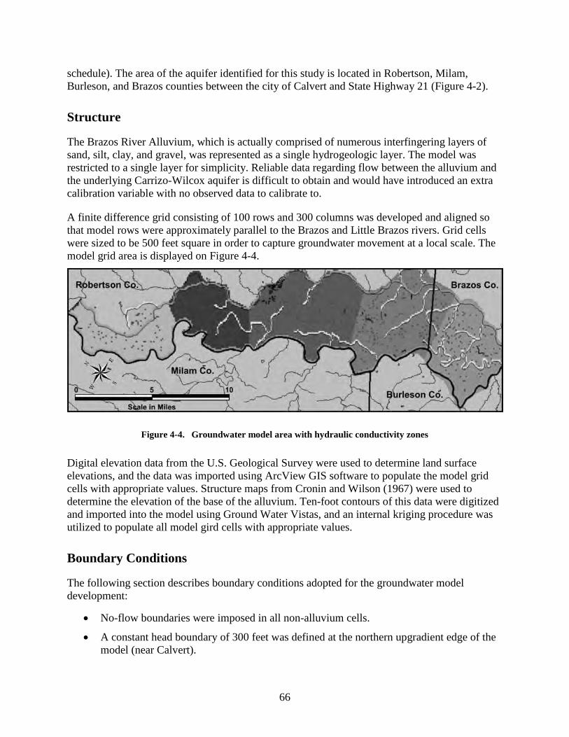
66

schedule). The area of the aquifer identified for this study is located in Robertson, Milam, Burleson, and Brazos counties between the city of Calvert and State Highway 21 (Figure 4-2).

Structure

The Brazos River Alluvium, which is actually comprised of numerous interfingering layers of sand, silt, clay, and gravel, was represented as a single hydrogeologic layer. The model was restricted to a single layer for simplicity. Reliable data regarding flow between the alluvium and the underlying Carrizo-Wilcox aquifer is difficult to obtain and would have introduced an extra calibration variable with no observed data to calibrate to.

A finite difference grid consisting of 100 rows and 300 columns was developed and aligned so that model rows were approximately parallel to the Brazos and Little Brazos rivers. Grid cells were sized to be 500 feet square in order to capture groundwater movement at a local scale. The model grid area is displayed on Figure 4-4.

Figure 4-4. Groundwater model area with hydraulic conductivity zones

Digital elevation data from the U.S. Geological Survey were used to determine land surface elevations, and the data was imported using ArcView GIS software to populate the model grid cells with appropriate values. Structure maps from Cronin and Wilson (1967) were used to determine the elevation of the base of the alluvium. Ten-foot contours of this data were digitized and imported into the model using Ground Water Vistas, and an internal kriging procedure was utilized to populate all model gird cells with appropriate values.

Boundary Conditions

The following section describes boundary conditions adopted for the groundwater model development:

• No-flow boundaries were imposed in all non-alluvium cells.

• A constant head boundary of 300 feet was defined at the northern upgradient edge of the model (near Calvert).

67

• The MODFLOW General Head Boundary (GHB) package was used to simulate the southeastern downgradient edge of the model (near Highway 21) with an assigned head of approximately 205 feet above mean sea level.

• The Brazos River and the Little Brazos River were represented using MODFLOW’s River Package. A free water surface two feet higher than the stream bed surface elevation was assigned in both rivers.

• MODFLOW’s Drain Package was used to simulate small ephemeral creeks on the alluvium surface that might be supplied by discharge from the alluvium under high water table conditions.

• MODFLOW’s Well Package was used to simulate existing irrigation wells within the model area as well as the enhanced recharge and recovery operations.

• MODFLOW’s Recharge package was used to simulate direct recharge to the aquifer surface from precipitation. An initial estimate of eight percent of precipitation based on Cronin and Wilson (1967) was reduced to four percent of precipitation during model calibration.

• Evapotranspiration was simulated using MODFLOW’s ET Package.

Aquifer Parameters

Hydraulic conductivity was represented using five different zones, varying from 100 to 200 feet per day, based on examination of well test data available in Cronin and Wilson (1967) (Figure 4-4).

A storage coefficient (specific yield) of 0.15 was used for the model. This is a typical storage coefficient used to represent water table conditions and is corroborated by Cronin and Wilson (1967).

Well pumpage values for the irrigation supply wells in the model were generated by evaluating aquifer use totals by county and then applying a typical irrigation use pattern with adjustments made for unusual precipitation conditions. A basic monthly water use distribution for the Brazos River Basin was modified to take into account rainfall totals during the calibration period. In months where the actual rainfall received was significantly less than the average rainfall for that month, the pumpage distribution factor for that month was increased to allow for greater pumpage. Conversely, in months where the actual rainfall received was significantly greater than the average rainfall for that month, the pumpage distribution factor for that month was decreased.

As mentioned previously, recharge was initially assigned a value of eight percent of precipitation measured at the College Station rain gage. This value was adjusted downward to four percent of precipitation during calibration.

Evapotranspiration rates used for the model area were derived from the Priestly-Taylor method, and an annual time series of twelve monthly values was applied to the model for the runs. Evaporation rates varied from approximately 5.2×10-3 feet per day (1.6 millimeters per day) to 2.6×10-2 feet per day (8 millimeters per day). The extinction depth was set at 15 feet.

68

The river package in MODFLOW simulates hydrologic interaction between rivers and the surrounding aquifer. Flow to and from the rivers is based on head differences between the river stage and the groundwater level in the model cell containing the river. Data required are the elevation of the stream bed, the stage elevation of the stream, the thickness of the river bed, and hydraulic conductivity of the stream bed sediments. River bed conductance is a calculated parameter which controls the flux rate of water between the river and the aquifer. The Brazos and Little Brazos rivers were represented as having a river stage of two feet during the course of the model runs. Initial estimates of conductance ranged from 2.0×104 to 2.0×105 square feet per day and were adjusted during calibration.

The drain package in MODFLOW allows water to be drained from the model through other mechanisms. This package may be used to represent a variety of physical situations. For this model, the drain package was used to represent the occurrence of high groundwater table conditions recharging ephemeral stream beds, whereupon the water lost from the aquifer would flow from these stream beds into the larger river system.

Model Calibration Once the basic data sets were assembled, a steady state version of the model was run. Average data values were used for all packages which had annual time series (well, recharge, and evapotranspiration). The purpose of this model run was to develop “average” starting heads for use in transient simulations and to perform initial calibration prior to the start of the transient calibration runs.

After the steady-state model had been successfully run, a transient model was developed which utilized monthly stress periods so that the seasonal irrigation patterns of groundwater pumpage and recharge could be simulated. The calibration period selected for this model was from January 1987 to December 1992. This period was selected because groundwater pumpage data, well water level data, precipitation data, and streamflow data were readily obtainable. In addition, during this time period, a majority of the wells within the study area displayed a decreasing water level from the period 1987 to 1990 and then an increasing water level from 1990 to 1992. It was determined that this cycle (a decreasing water level rebounding in the latter part of the calibration period) would provide an opportunity to calibrate the model to both rising and falling water level conditions.

Eleven wells in the model area, which are regularly monitored for water levels by the TWDB, were selected as calibration targets. Water-level data were obtained from the database available on the TWDB Web page. These wells are broadly spaced and represent a reasonably homogeneous spatial distribution within the model area. Calibration target well locations are shown in Figure 4-5. Each of these wells had between four and seven recorded water levels during the calibration period for a total of 121 separate calibration target water levels.

During calibration, the initial recharge estimate was reduced from eight percent to four percent of precipitation. The initial estimate of 8 feet for evapotranspiration extinction depth was increased to 15 feet, which is consistent for values used in sandy soils in other Central Texas

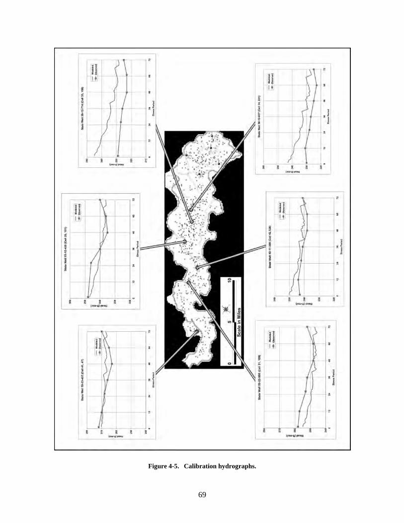
69

Figure 4-5. Calibration hydrographs.

70

Figure 4-5. Continued.

71

groundwater models. The values for river bed conductance, which originally ranged from 2.0×104 to 2.0×105 square feet per day, were adjusted upward during calibration.

Calibration is often guided by examination of the total residuals of the model run. A residual is the difference between the field measurement and the model-computed value. A summary of the residual statistics for the Brazos River Alluvium model calibration is presented in Table 4-1. The mean residual for all 121 calibration targets was -3.4 feet. A plot of observed versus simulated heads is displayed in the upper plot of Figure 4-6. For reference, the diagonal line drawn across the graph represents a perfect match between observed and computed head values. This graph displays a reasonable correspondence between the observed and model-computed values. The lower plot in Figure 4-6 presents another representation of the calibration results, plotting observed head values versus the corresponding residual value. This graph makes it apparent that most of the calibration residuals are negative, indicating that, for the most part, the computed values are higher than field-measured values.

Table 4-1. Residual statistics for the Brazos River Alluvium model calibration.

Residual Mean -3.43 Res. Std. Dev. 4.65 Sum of Squares 2301 Abs. Res. Mean 4.57 Min. Residual -15.98 Max. Residual 5.01 Head Range 67.00 Std/Head Range 6.94%

Conjunctive Use Testing Applications Once the model was sufficiently calibrated to represent observed groundwater levels, model simulations were set up to test the feasibility of a conjunctive use project in the aquifer system. The conjunctive use project that was simulated was designed to be consistent with the water supply project outlined in Chapter 5.19 of the 2001 Brazos G Regional Water Plan, “Conjunctive use of the Brazos River alluvium” (HDR Engineering and others, 2001). The referenced chapter summarizes the project description, design calculations, cost estimates, and environmental implications of a project that would divert high river flows from the Brazos River to a series of infiltration basins or injection wells on the alluvium surface.

A note should be made regarding the semantics of the following discussion. The project as proposed recommends using infiltration basins to enhance recharge to the aquifer. In the model, however, the enhanced recharge is simulated using injection wells in the well package. This was done simply because it is easier to use the well package than the recharge package to create and manipulate the necessary MODFLOW data files. It is irrelevant to the model whether the well package or recharge package is used—the water is delivered either way. For the purposes of this report, however, enhanced recharge will heretofore be referred to as “injection” and recovery will be referred to as “extraction”.

72

Figure 4-6. Observed water levels versus residuals.

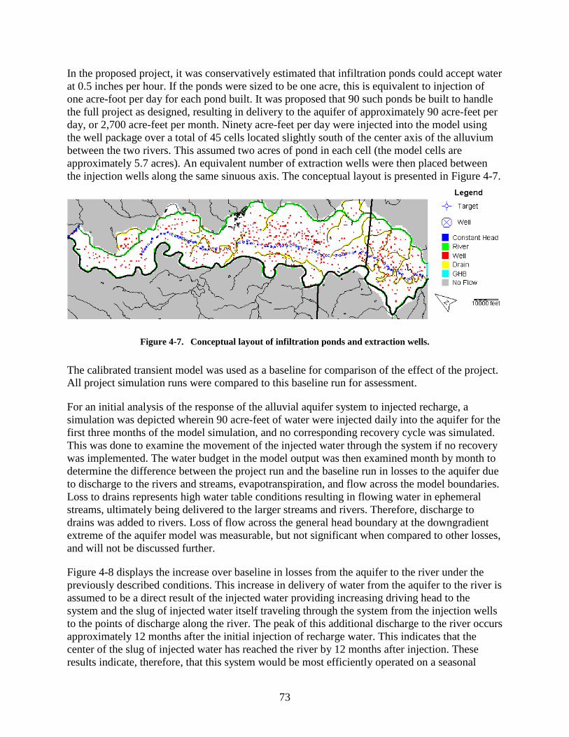
73

In the proposed project, it was conservatively estimated that infiltration ponds could accept water at 0.5 inches per hour. If the ponds were sized to be one acre, this is equivalent to injection of one acre-foot per day for each pond built. It was proposed that 90 such ponds be built to handle the full project as designed, resulting in delivery to the aquifer of approximately 90 acre-feet per day, or 2,700 acre-feet per month. Ninety acre-feet per day were injected into the model using the well package over a total of 45 cells located slightly south of the center axis of the alluvium between the two rivers. This assumed two acres of pond in each cell (the model cells are approximately 5.7 acres). An equivalent number of extraction wells were then placed between the injection wells along the same sinuous axis. The conceptual layout is presented in Figure 4-7.

Figure 4-7. Conceptual layout of infiltration ponds and extraction wells.

The calibrated transient model was used as a baseline for comparison of the effect of the project. All project simulation runs were compared to this baseline run for assessment.

For an initial analysis of the response of the alluvial aquifer system to injected recharge, a simulation was depicted wherein 90 acre-feet of water were injected daily into the aquifer for the first three months of the model simulation, and no corresponding recovery cycle was simulated. This was done to examine the movement of the injected water through the system if no recovery was implemented. The water budget in the model output was then examined month by month to determine the difference between the project run and the baseline run in losses to the aquifer due to discharge to the rivers and streams, evapotranspiration, and flow across the model boundaries. Loss to drains represents high water table conditions resulting in flowing water in ephemeral streams, ultimately being delivered to the larger streams and rivers. Therefore, discharge to drains was added to rivers. Loss of flow across the general head boundary at the downgradient extreme of the aquifer model was measurable, but not significant when compared to other losses, and will not be discussed further.

Figure 4-8 displays the increase over baseline in losses from the aquifer to the river under the previously described conditions. This increase in delivery of water from the aquifer to the river is assumed to be a direct result of the injected water providing increasing driving head to the system and the slug of injected water itself traveling through the system from the injection wells to the points of discharge along the river. The peak of this additional discharge to the river occurs approximately 12 months after the initial injection of recharge water. This indicates that the center of the slug of injected water has reached the river by 12 months after injection. These results indicate, therefore, that this system would be most efficiently operated on a seasonal

74

Figure 4-8. Increased river losses due to enhanced recharge slug.

basis, injecting water during the spring and extracting it for delivery during the summer of the same year. If the injected water were not recovered in this time frame, it would gradually be lost to the surrounding natural system. This finding indicates that this conjunctive use project would not be appropriate for long-term storage to be recovered during periodic drought conditions.

Figure 4-9 displays the increase over baseline in losses from the aquifer to evapotranspiration. The injected water raises the water table locally, subjecting it to greater losses from evapotranspiration than would otherwise occur. Note that evapotranspiration losses are cyclical, peaking in the hot summer months and becoming less during the winter. An interesting result that was encountered during initial evapotranspiration tracking runs concerned the location of the injection/extraction well system. Initially the injection/extraction wells were placed in the approximate center of the widest area of the alluvium with the expectation that maximizing the distance from the rivers would be most efficient for preventing losses to the river. However, this resulted in evapotranspiration losses five to six times greater than those represented in Figure 4-9. Upon further inspection of the model graphics and underlying geologic data, it was noted that although the initial well placement maximized distance from the rivers, depth to water was shallower in this area than it was further southwest, closer to the Brazos River. In many instances the initial depth to water prior to injection was fifteen feet or less. Since the depth of influence of evapotranspiration in the model is fifteen feet, this resulted in essentially all of the injection

75

Figure 4-9. Increased evapotranspiration losses due to enhanced recharge slug.

being immediately subject to evapotranspiration losses. In fact, the thickness of the alluvial deposits in the valley is asymmetric, with the deposits considerably thicker near the Brazos River than the Little Brazos River. By moving the injection wells just a little closer to the Brazos River, where there was more “freeboard” between the land surface and the water table, evapotranspiration losses were significantly reduced. Another significant finding is implied in Figure 4-9. As mentioned previously, the evapotranspiration losses from the conjunctive use system are highest during the summer months. However, these are the same months when the extraction wells would be recovering water from the aquifer for delivery to the river. Extraction cycles would reduce the water table in the area, thus reducing evapotranspiration losses during these months.

Conjunctive Use Operational Simulations To test the effect of operating a conjunctive use project of the Brazos River and the Brazos River Authority, a test case was set up in which the same amount of water (90 acre-feet per day) was injected in the first three months of each year. Extractions were scheduled to take place during June, July, and August of each year. Considering the supply of water in the Brazos River Alluvium and the conjunctive use project, potentially more water may be recovered from the

76

system than was initially injected, due to the presence of pre-existing groundwater reserves at the project site and to the dynamic nature of the natural recharge processes. To evaluate the behavior of the system under different extraction schedules, four test runs were made in which 90 percent, 100 percent, 110 percent, and 125 percent of the amount injected was extracted. These runs are referred to as Tests 1, 2, 3, and 4.

To demonstrate the general effect of the conjunctive use storage and recovery cycles on water levels within the model area, water levels were monitored in two wells during the baseline simulation and with the four test projects. Test 3, where extractions were 110 percent of injections, was chosen as being representative of the general response of the aquifer to a conjunctive use project. The comparative hydrographs for the two wells (59-20-820 and 59-11-308) are displayed in Figure 4-10. In both cases, the results indicate that the cyclical operations would cause short-term water level fluctuations above and below the baseline levels by no more than one to two feet in most cases. Water levels which are elevated above the baseline during the injection cycle are routinely pulled below the baseline levels during the extraction cycle.

Figure 4-11 demonstrates the change in losses to the aquifer over time as compared to the baseline conditions. It is analogous to Figure 4-8, except that the model run simulated six successive years of recharge and recovery cycles. The primary y-axis represents the change over the baseline run in losses to the aquifer system expressed as a percentage of the quantity of water injected. The cycles of injection and extraction are depicted on the secondary y-axis for a time reference. The primary message of this figure is that the greatest losses of this system, and thus the peak inefficiency, occur in the first year of operation when the change in losses over the baseline are over 13 percent of the total quantity injected. This occurs when the project is introducing a large amount of water to an aquifer system that was previously in relative equilibrium and when the water levels were relatively high. With each succeeding year, the losses are reduced as the system moves toward a new stable equilibrium until losses stabilize at approximately two percent of the quantity injected at the end of the 6-year simulation. This “equilibrium efficiency” was lower for the model runs with greater extraction quantities, ranging from five percent for the Test 1 scenario to nearly zero percent for the Test 4 scenario. In other words, the losses form the most aggressive extraction schedule were the closest to the losses calculated in the baseline run. Of course, in the test runs that extracted greater amounts of water, a greater amount of groundwater is removed from storage, and resulting water levels are slightly lower. However, all achieved approximate equilibrium by the end of the six-year run.

Table 4-2 compares the effect of the various test scenarios on cumulative water budget values in comparison to the baseline calculated losses. Note that as the volume of water extracted in the test runs increases, the losses to evapotranspiration and river leakage decrease. This is indicative of the fact that the extraction wells are capturing a quantity of water that otherwise would be lost from the system and is a partial explanation of the phenomenon previously described, wherein higher extraction rates lead to lesser losses from the aquifer in comparison to the baseline.

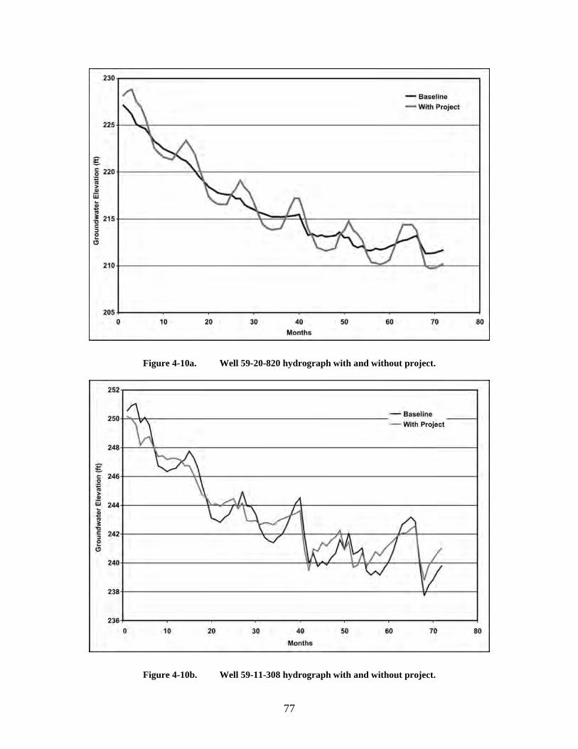
77

Figure 4-10a. Well 59-20-820 hydrograph with and without project.

Figure 4-10b. Well 59-11-308 hydrograph with and without project.

78

Figure 4-11. Operational losses of enhanced recharge water to natural system.

Table 4-2. A comparison of cumulative water budget values from model test scenarios to baseline calculated values.

Baseline Test 1 Test 2 Test3 Test 4 Injection 0 48600 48600 48600 48600 Extraction 0 43740 48600 53460 60750 Evapotranspiration 193414 1136 900 707 528 River Leakage 39851 1570 843 280 -234 Drains 323 17 10 4 -2 Upgradient Boundary 1570 0 0 0 0 Downgradient Boundary 2729 -19 -58 -98 -157 Notes: All values in acre-feet, and values are cumulative at end of six-year test period. + indicates greater than baseline. - indicates less than baseline.

79

Conclusions The modeling analysis of conjunctive use projects in the Brazos River Alluvium aquifer conducted for this report indicates that the groundwater system studied appears to be suitable for use as a site for a conjunctive use water supply project in the future. Specific findings produced by the model are:

• The travel time for water placed into aquifer storage at the locations indicated in this report is on the order of one year. Thus, the storage/recovery operational cycles should be timed to recover water on a seasonal basis (that is, perform recovery operations less than one year after the storage injection takes place). This will prevent unnecessary losses from the system through leakage to the river.

• Evapotranspiration losses were significantly greater if the infiltration ponds and supply wells were located over areas with shallow water table than a deeper water table. Greater efficiency is obtained from the system by placing wells in areas which maximize “freeboard,” or unsaturated zone thickness, rather than by placing them in areas which maximize distance between infiltration ponds and the zones of discharge along the river.

• If extraction and recovery are performed on a seasonal basis, there is little long-term effect on water levels. Temporary fluctuations of water levels due to injection/extraction cycles were only a few feet above and below baseline conditions, even when extraction rates exceeded injection rates.

• The system tends toward greater stability and efficiency with repeated operation. The initial flux of injection water induces a condition of disequilibrium on an aquifer system that was previously in equilibrium. Within the six-year period, the system re-achieves stable equilibrium efficiency. In fact, this efficiency is higher for the recovery schedules which extracted greater quantities of water than were injected, partly due to the capture of water that otherwise would be lost to evapotranspiration and river leakage during the summer months.

References Cronin, J., and Wilson, C., 1967, Ground water in the flood plain alluvium of the Brazos River,

Whitney Dam to the vicinity of Richmond, Texas: Texas Water Development Board Report 41.

HDR Engineering, 2001, Brazos River alluvium groundwater model and conjunctive use analysis—Final report: prepared for the Texas Water Development Board.

HDR Engineering, Freese and Nichols, R.W. Harden & Associates, Hicks and company, Capital City Consulting, Texas Agricultural Experiment Station, and Texas Rural Water Association, January 2001, Brazos G Regional Water Planning Area Regional Water Plan: prepared for Brazos G Regional Water Planning Group, with administration by Brazos River Authority.

Texas Water Development Board Groundwater Database, 1999, available at (http://www.twdb.state.tx.us/GwRD/waterwell/well_info.asp).

80

This page intentionally blank.

81

Chapter 5

Hydrochemistry, Salinity Distribution, and Trace Constituents: Implications for Salinity Sources,

Geochemical Evolution, and Flow Systems Characterization, Gulf Coast Aquifer, Texas

Ali H. Chowdhury1, Radu Boghici1, and Janie Hopkins1

Introduction Groundwater is a valuable resource to the fast growing communities along the Texas Gulf Coast. Recurrent drought conditions, historical and current overpumping of the aquifer in excess of natural replenishment through recharge, and limited availability place an ever increasing demand on this resource. Over 1.1 million acre-feet of groundwater are annually used from the Gulf Coast aquifer in Texas. The Gulf Coast aquifer extends over 430 miles from the Texas-Louisiana border in the northeast to Texas-Mexico border in the south. The Gulf Coast aquifer is comprised of fluvial-deltaic sediments that thin in the outcrop areas and progressively thicken to several thousand feet near the coast. Repeated sea-level changes and natural subsidence of the basin due to sediment loading produced a complex set of discontinuous bodies of sand, silt, clay, and gravel in the Gulf Coast. Lateral and vertical discontinuity and interfingering of these sand and clay bodies compartmentalize the flow systems with potential for little hydraulic interconnection between them. Furthermore, numerous growth faults that occur parallel to the coast exert additional complexity to the groundwater flow system. Significant quantities of groundwater occur in the Gulf Coast aquifer in sections where sands are dominant. However, some of this resource is not directly usable due to its moderate to high salinity. In most of the outcrop, groundwater is generally fresh. Groundwater increases in salinity at depth and along flow paths towards the coast. Groundwater salinity also increases from the northern humid areas to the southern semi-tropical and semi-arid areas of the Texas Gulf Coast.

Groundwater pumping in the Gulf Coast aquifer caused water-level declines of more than 350 feet in some areas, produced compaction of clay and shale beds contained within the aquifer materials, and subsequently caused land-surface subsidence in or near the cones of depression. Salt domes that pierce through the aquifer at different depths affect groundwater salinity in their vicinity. In addition, formation brines from the deeper subsurface may flow upward along faults or due to an increase in hydraulic pressure gradients affecting groundwater composition in

1 Texas Water Development Board

82

shallow aquifers. A lowering of the hydraulic gradient due to over-pumping in areas near the coast may locally cause saltwater intrusion. In this paper, we will (1) describe spatial and depth distributions of salinity; (2) identify sources and geochemical processes that gave rise to this salinity; (3) describe spatial and depth distributions of arsenic and identify its origin; (4) describe spatial and depth distributions of alpha, beta, and radon-222 activities and identify their origin; and (5) evaluate changes in groundwater salinity with water-level declines in or near the cones of depression. We discuss each of the above topics under separate sections.

Stratigraphy and Mineralogy The Gulf Coast aquifer in Texas consists of five hydrostratigraphic units (from oldest to youngest): (1) the Catahoula Tuff or Sandstone, (2) the Jasper aquifer, (3) the Burkeville confining system, (4) the Evangeline aquifer, and (5) the Chicot aquifer (Baker, 1979). The Catahoula Tuff or Sandstone mainly consists of pyroclastic and tuffaceous sandstone; the Jasper aquifer mainly contains the Fleming and the Oakville formations, consisting of interbedded sand and clay; the Burkeville confining system consists mainly of silt and clay; the Evangeline aquifer has a high sand-clay ratio and contains sand beds tens of feet thick; and the Chicot aquifer contains sand, clay, and gravel (Baker, 1979).

Sediments of the Gulf Coast aquifer were deposited in a fluvial-deltaic or shallow marine environment (Sellards and others, 1932). Repeated sea-level transgression and regression and basin subsidence caused development of cyclic sedimentary deposits composed of discontinuous sand, silt, clay, and gravel (Sellards and others, 1932; Kasmarek and Robinson, 2004). Most of the sediments of the Gulf Coast aquifer thicken towards the Gulf of Mexico. Faults that remained active during sedimentation (growth faults) contributed to additional sediment thickness over short lateral distances (Verbeek and others, 1979). Kreitler and others (1977) observed appreciable vertical displacement and abrupt thickening of the Alta Loma Sand, placed at the base of the Chicot aquifer in Harris and Galveston counties, which they attributed to faults. They suggested that the fault zone that occurs between Harris and Galveston counties acts as a partial hydrologic barrier separating the two partially independent flow systems and controlling groundwater composition between these two counties. In addition, complexity of the Gulf Coast aquifer is further advanced by numerous clay layers less than six feet thick contained within the water-bearing units of the sand beds that retard vertical movement locally and may provide different hydraulic heads to each sand bed (Gabrysch, 1984).

Numerous salt domes occur in the Gulf Coast aquifer (Beckman and Williamson, 1990), some of which pierce through the shallow aquifers and reach near the land surface (Hamlin, this volume). Morton and others (1983) reported that salt domes are abundant along the northern part and nearly absent along the southern part of the Texas Gulf Coast.

In order to explain geochemical conditions for paragenesis of diagenetic minerals in the Oakville Formation sand, Galloway (1982) postulated three hydrogeologic regimes: (1) the meteoric regime that surrounds the basin margins where surface water infiltrates into the permeable strata and moves in response to gravitation heads; (2) the elisian or compactional regime that expels upward to outward connate water contained within the fine-grained sediments caused by compressible or lithostatic stresses; and (3) the abyssal regime in the deep core of the basin fill

83

that provides significant volumes of water due to permeability reduction by compaction, cementation, and mineral dehydration reactions. Of these three regimes, the meteoric regime is most dynamic, with several geochemical trends observed along flow paths: bicarbonate increases moderately, chloride and total dissolved solids increase markedly, sodium to calcium ratios increase with a reduction in calcium concentrations, pH decreases gradually, and Eh commonly decreases abruptly. Galloway (1982) suggested that uranium mineralization in the Oakville Formation and underlying Catahoula aquifers was caused by migration of compactional fluids along deep-seated growth faults.

Mineralogical compositions of the Miocene-Pliocene sandstones that form the Gulf Coast aquifers in Texas are poorly known. However, numerous investigations have been carried out to determine mineralogical compositions of the Oligocene sandstones from the Frio and the Catahoula formations (Loucks and others, 1979; Galloway, 1982). Quartz percentage in these sandstones increases from 20 to 60 percent at the southern part of the Texas Gulf Coast to 50 to 85 percent at the northern part of the Texas Gulf Coast (Lindquist, 1977; Loucks and others, 1981). Feldspar decreases from 20 to 50 percent to 10 to 30 percent in the same direction. Sandstones along the lower coast are rich in volcanic and carbonate rocks occasionally containing caliche fragments (Lindquist, 1977). Carbonate rock fragments decrease and metamorphic rock fragments increase towards the middle coast. Volcanic rocks dominate again in the upper coast (Lindquist, 1977). McBride and others (1968) suggest that the lower Catahoula Formation in northern Fayette County contains mainly tuff, with volcanic conglomerate and sandstones dominant in the mid-section. Bentonite and alteration products of volcanic glass (zeolite, calcium-montmorrilonite, and chalcedony) are widespread throughout the formation. Caliches are common near the surface, which suggests that the land surface was occasionally exposed to soil forming processes (McBride and others, 1968). Hoel (1982) observed that the Goliad Formation is genetically and compositionally similar to the Catahoula and the Oakville sandstones and contains a large proportion of orthoclase and plagioclase feldspars and volcanic rock fragments, particularly south of the San Patricio-Refugio county line. Sellards and others (1932) report that the Goliad Sand in South Texas is cemented by caliche containing more than 30 percent calcium carbonate. Gabrysch and Bonnet (1975) analyzed the mineralogical composition of the clay beds and observed montmorillonite to be the main constituent of the clay with minor amounts of illite, chlorite, and kaolinite.

Water Levels and Regional Groundwater Flow A water table is generally a subdued replica of the land surface. Under topographic highs where recharge occurs, water levels occur at shallow depths under unconfined conditions. Recharge waters in the outcrop are typically fresh and reflect composition of the rainwater, except in arid and semi-arid areas, where rainwater dissolves salts from the soils and percolates to the groundwater in the outcrop. As the aquifer dips beneath lower permeability sediments, groundwater becomes confined under increasing hydrostatic pressure due to the presence of impermeable fine-grained clays and silts. In topographic lows (discharge areas), groundwater flow is directed upward as a result of artesian pressure exceeding local hydrostatic pressure. Groundwater becomes more saline in the deeper subsurface and in discharge areas due to its long residence time and continued reaction with the aquifer minerals.

84

Water-level maps for the Chicot, Evangeline, and the Jasper aquifers show that regional groundwater flow is directed east towards the Gulf of Mexico (Figures 5-1, 5-2, and 5-3). We note that groundwater pumping has caused significant water-level decline in parts of the Gulf Coast aquifer (Figures 5-1 and 5-2). For example, water-level measurements from 2001 to 2005 show the presence of large cones of depression in Harris and Kleberg counties (Figure 5-2). Major cones of depression change regional groundwater flow direction wherein groundwater from the outcrop is diverted towards the center of the cone as opposed to allowing it to flow towards the Gulf of Mexico (Figures 5-1 and 5-2). Hydrographs of selected wells from areas

Figure 5-1. Water-level elevations and regional groundwater flow directions in the Chicot aquifer (includes water-level measurements from 2001 to 2005).

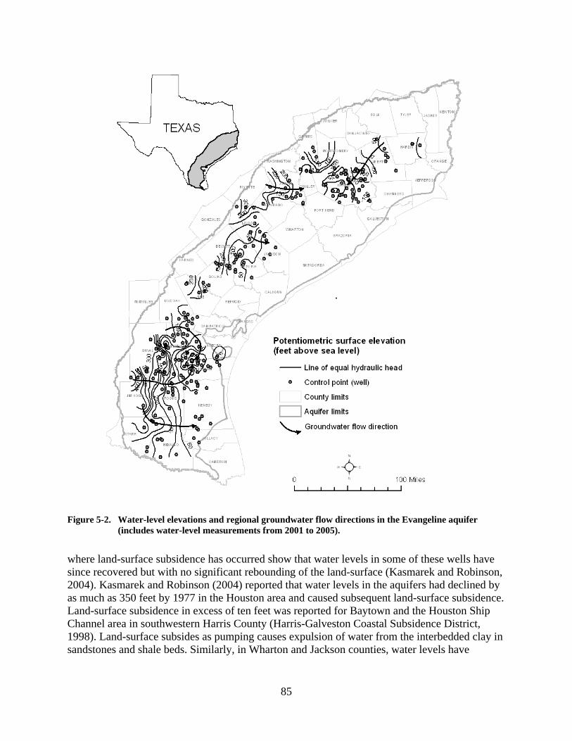
85

Figure 5-2. Water-level elevations and regional groundwater flow directions in the Evangeline aquifer (includes water-level measurements from 2001 to 2005).

where land-surface subsidence has occurred show that water levels in some of these wells have since recovered but with no significant rebounding of the land-surface (Kasmarek and Robinson, 2004). Kasmarek and Robinson (2004) reported that water levels in the aquifers had declined by as much as 350 feet by 1977 in the Houston area and caused subsequent land-surface subsidence. Land-surface subsidence in excess of ten feet was reported for Baytown and the Houston Ship Channel area in southwestern Harris County (Harris-Galveston Coastal Subsidence District, 1998). Land-surface subsides as pumping causes expulsion of water from the interbedded clay in sandstones and shale beds. Similarly, in Wharton and Jackson counties, water levels have

86

Figure 5-3. Water-level elevations and regional groundwater flow directions in the Jasper aquifer (includes water-level measurements from 2001 to 2005).

declined by more than 50 feet (Chowdhury and others, 2004). Farther south in Kleberg County, water levels have declined historically by as much as 200 feet (Shafer and Baker, 1973).

Groundwater Composition Groundwater composition commonly retains unique chemical signatures of a flow system. These diagnostic signatures help define groundwater flow behavior as groundwater moves from the recharge areas in the outcrop, downward to the deeper subsurface, and upward to the discharge

87

areas near the coast. Differences in groundwater composition along flow paths help us interpret and verify flow systems, identify water sourced under various recharge conditions, and understand geochemical evolution of the water. Final groundwater composition ultimately depends on a multitude of factors that may include hydraulic characteristics and mineralogy of the aquifer materials, relative rates of mineral dissolution and precipitation reactions, cation exchanges, mixing of waters of various origins, redox reactions, and groundwater residence times in the aquifer.

Major Elements

Major elements consisting of calcium, sodium, potassium, magnesium, bicarbonate, chloride, and sulfate typically comprise more than ninety-five percent of the groundwater composition. These elements are non-conservative as they participate in and are subject to changes in concentrations due to geochemical reactions. Major elements in groundwater are derived from solute concentrations in the precipitation, water-rock interactions in the soil zone above the water table, and mineral reactions in the saturated zone below the water table. Progress or extent of chemical reactions along flow paths can therefore be identified by observing changes in absolute concentrations or relative element ratios from their initial compositions in the outcrop. In most cases, groundwater movement down flow paths follows a sequence of geochemical reactions that may provide information on chemical maturity and relative residence times of the ground water (Herczeg and Edmunds, 2000). Molar ratios of several elements including Na/Cl, SO4/Cl, Mg/Ca, K/Na, Ca/Na, and Ca+Mg/SO4 ratios are used to determine geochemical evolution of groundwater (Richter and Kreitler, 1991; Herczeg and Edmunds, 2000; Cartwright and others, 2004).

Methods

We analyzed chemical compositions of about six hundred groundwater samples from the Texas Water Development Board’s (TWDB) groundwater database. For this study, we considered samples collected during 2001 through 2005. This time period was chosen because extensive sampling of the Gulf Coast aquifer was undertaken during this period and this dataset should adequately represent current groundwater compositions in the Gulf Coast aquifer. However, adequate sample coverage was missing for Harris County during 2001 through 2005. Therefore, we included additional samples analyzed during 1997 to increase sample coverage for Harris County. All groundwater samples were analyzed by ion chromatography-mass spectrometry (ICP-MS) for major and trace elements at the Lower Colorado River Authority’s Environmental Laboratory.

We described groundwater salinity based on total dissolved solids (TDS) concentration of the waters: fresh (less than 1,000 milligrams per liter [mg/l]), slightly saline (1,000 to 3,000 mg/l), moderately saline (3,000 to 10,000 mg/l), very saline (10,000 to 35,000 mg/l), and brine (greater than 35,000 mg/l) (Winslow and Kister, 1956). TDS represents the total amount of solids that remain in water after the sample is evaporated to dryness. Salinity essentially means the same as total dissolved solids. We plotted the major elements and their ratios for identifying geochemical processes and identify sources of salinity. We plotted groundwater compositions into Piper diagrams to group groundwater into distinct water types or chemical facies (Piper, 1944).

88

Results

Groundwater composition in the Gulf Coast aquifer in Texas is highly variable. Groundwater composition is generally fresh in the outcrop and becomes more saline near the coast. Of the six hundred samples that we analyzed, we observed that about seventy percent of the samples in the Chicot and the Evangeline aquifers and eighty-five percent of the samples in the Jasper aquifer have fresh water. Nearly all of the remaining samples are slightly saline (Table 5-1).

Table 5-1. Water quality types in the Chicot, Evangeline, and Jasper aquifers.

Aquifer Water quality (percent total)Fresh Slightly saline Moderately saline

Chicot 72 26 2Evangeline 70 28 2Jasper 85 13 1

Groundwater is relatively more saline in the central and southern parts compared to the northern part of the Gulf Coast aquifer (Figures 5-4, 5-5, and 5-6).

In order to better understand geochemical processes that gave rise to groundwater salinity, we examined spatial distribution of the major elements across the Gulf Coast aquifer. Details on this distribution are presented elsewhere (Chowdhury and others, in prep.). We observed that bicarbonate concentrations generally increase along flow paths with an abrupt increase in their concentration along the coast in Matagorda and Brazoria counties (Figure 5-7). To the south, bicarbonate shows a decrease along flow paths in Kenedy and Cameron counties. Sulfate concentrations do not vary significantly along flowpaths, but higher concentrations of sulfate occur in the south than the northern part of the Gulf Coast aquifer (Figure 5-8). Sodium and chloride concentrations increase along flow paths, and their concentrations significantly increase in the southern part of the Gulf Coast aquifer (Figures 5-9 and 5-10).

We used molar ratios of Na/Cl to determine sources of Na ions and identify geochemical processes that affect Na concentrations. Halite contains Na and Cl in equal concentrations. Therefore, groundwater affected by halite dissolution should typically contain molar Na/Cl ratios equal to 1 unless the ratio is affected by cation exchange reactions. Molar Na/Cl ratios in sea water is about 0.85 and the ratio in deep-basin brines is less than 0.5 (Richter and Kreitler, 1991). In the Gulf Coast aquifer, we observe that the molar Na/Cl ratios range from 0.49 to 5.98 (1.77 ± 0.94), 0.4 to 10.95 (2.03 ± 1.57), and 0.6 to 41.94 (3.58 ± 5.48) for the Chicot, Evangeline, and Jasper aquifers, respectively. Molar ratios of Na/Cl increase from the shallower to the deeper aquifers which is probably caused by progressive cation exchanges and/or mixing of saline water from the deeper subsurface (Table 5-2). Variability in the Na/Cl ratios increases with depth, as reflected by increases in standard deviations from the Chicot to the Jasper aquifers. Spatial distributions of molar Na/Cl ratios indicate that several samples, particularly in the northern part of the Gulf Coast aquifer in the vicinity of the salt diapers, have molar Na/Cl ratios close to 1 (Figure 5-11). Most of the groundwater in the Gulf Coast aquifer has molar Na/Cl ratios that vary from 1 to 4 (Figure 5-11).

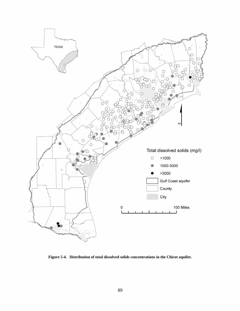
89

Figure 5-4. Distribution of total dissolved solids concentrations in the Chicot aquifer.

90

Figure 5-5. Distribution of total dissolved solids concentrations in the Evangeline aquifer.

91

Figure 5-6. Distribution of total dissolved solids concentrations in the Jasper aquifer.

92

Figure 5-7. Distribution of bicarbonate concentrations in the Chicot aquifer.

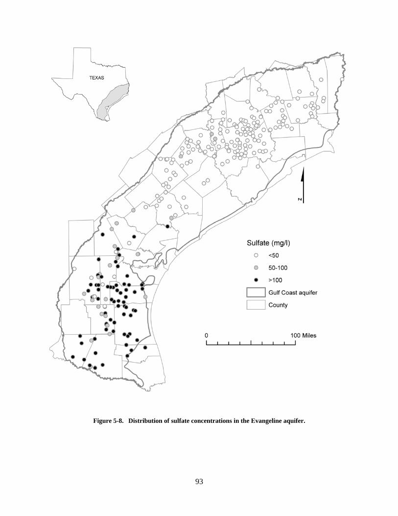
93

Figure 5-8. Distribution of sulfate concentrations in the Evangeline aquifer.

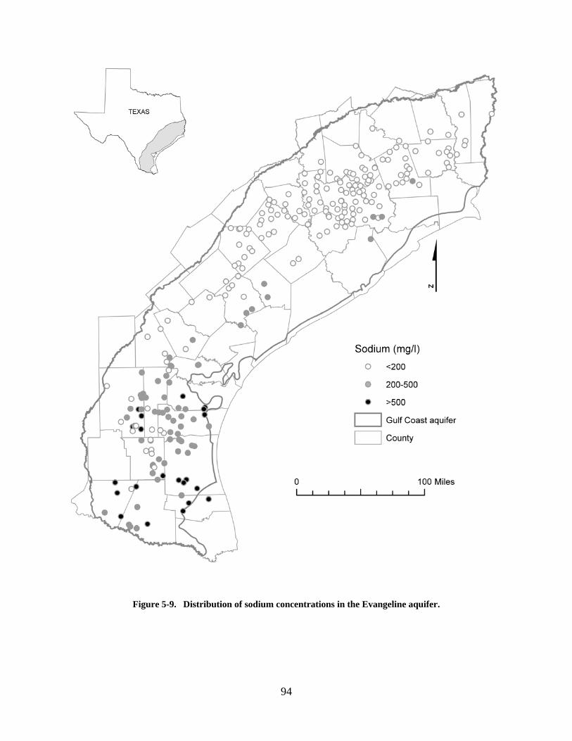
94

Figure 5-9. Distribution of sodium concentrations in the Evangeline aquifer.

95

Figure 5-10. Distribution of chloride concentrations in the Evangeline aquifer.

96

Figure 5-11. Distribution of Na/Cl molar ratios in the Gulf Coast aquifer of Texas.

Table 5-2. Concentrations of Na/Cl ratios in the Chicot, Evangeline, and Jasper aquifers.

Aquifer Molar Na/Cl ratios Range Mean Median Standard deviation Number of samples

ChicotEvangelineJasper

0.49 - 5.980.4 - 10.950.6 - 41.94

1.772.033.58

1.561.612.23

0.941.575.48

24025898

97

We used Piper diagrams to group groundwater from the Chicot, Evangeline, and Jasper aquifers into distinct chemical types. We observed that the analyzed samples in the Gulf Coast aquifer are mainly composed of Ca-HCO3, Ca-Na-HCO3-Cl, and Na-HCO3 type waters (Figure 5-12). Numerous samples fall along a straight line from the calcium to the sodium end of the cation triangle (Figure 5-9). Groundwater in the outcrop areas in the northern part are more commonly Ca-HCO3 types that evolve into mixed Ca-Na-HCO3-Cl water along regional flow paths and to Na-HCO3 water in the discharge areas near the coast. Groundwater composition in the central and the southern parts of the Gulf Coast aquifer changes to Na-Cl-HCO3 or Na-Cl-SO4 water along regional flow paths (Figures, 5-7, 5-8, 5-9, and 5-10). Relatively more samples from the Evangeline aquifer have higher concentrations of sulfate, sodium, and chloride (Figure 5-12b).

We used cross-plots of various ions to identify their sources. Plots of sodium and bicarbonate and sodium and calcium for 17 groundwater samples from Harris and Galveston counties show a correlation coefficient of 0.82 between sodium and bicarbonate and a correlation coefficient of -0.66 between sodium and calcium (Figures 5-13a and 5-13b). Bivariate plots of Na and Cl show good correlation coefficients of 0.85 and 0.87 for the Chicot and Jasper aquifers, respectively, and a moderate correlation coefficient of 0.59 for the Evangeline aquifer (Figures 5-14b, 5-15b, and 5-16b). Plots of Na/Cl ratios versus Cl show a decrease in Na/Cl ratios at higher Cl concentrations in a small number of samples (Figures 5-14c, 5-15c, and 5-16c). Plots of excess sodium from sources other than halite (Na-Cl) and excess calcium and magnesium (Ca+Mg-0.5HCO3-SO4) from sources other than carbonate and gypsum show near perfect correlation coefficients (r2 = 0.95, r2 = 0.98, and r2 = 0.98 for the Chicot, Evangeline, and Jasper aquifers, respectively; Figures 5-14d, 5-15d, and 5-16d).

Groundwater composition shows no trends in salinity changes with well depths (Figures 5-14a, 5-15a, and 5-16a). Many wells in the Chicot, Evangeline, and Jasper aquifers have groundwater compositions containing low dissolved solids (less than 300 mg/l) at depths of more than 2,000 feet.

Discussion

Salinity differences from the northern to the southern parts of the Gulf Coast aquifer are probably caused by several processes including recharge under different climatic conditions, variation in lithologic composition, ion-exchange reactions, saltwater intrusion, and retention of residual connate water. For example, annual average rainfall in the northern part of the Gulf Coast aquifer is about 56 inches, while in the central and the southern parts of the Gulf Coast aquifer annual rainfall gradually decreases to about 18 inches (Chowdhury and Mace, 2004). A higher evaporation rate in the central and southern parts of the aquifer, frequent occurrences of caliches, and salt accumulation in the soils further reduce potential for fresh rainwater infiltration into the groundwater. Therefore, it is no coincidence that the groundwater in the southern parts of the Gulf Coast aquifer has higher concentrations of sodium, chloride, and sulfate. In addition, differences in mineralogical compositions of the aquifer materials between the northern and the southern parts of the Gulf Coast contributed to varying groundwater composition. For example, sandstone compositions in the northern part are more commonly quartz arenite, while to the south, sandstone compositions are more likely arkosic and greywackes containing abundant feldspar and rock fragments. Varying chemical stability of the aquifer minerals will produce

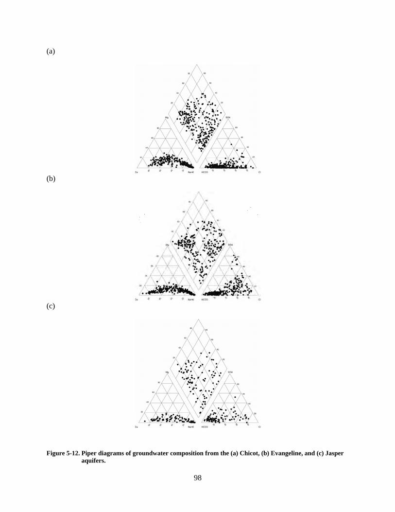
98

(a)

(b)

(c)

Figure 5-12. Piper diagrams of groundwater composition from the (a) Chicot, (b) Evangeline, and (c) Jasper aquifers.

99

Figure 5-13. Relationships between (a) Na and HCO3 and (b) Na and Ca in the Chicot aquifer in Harris and Galveston counties.

Figure 5-14. Relationships between (a) total dissolved solids and well depth, (b) Na and Cl, (c) Na/Cl and Cl, (d) Na-Cl and Ca+Mg-SO4-0.5HCO3, (e) Br and Cl, and (f) Br/Cl and Cl for the Chicot aquifer.

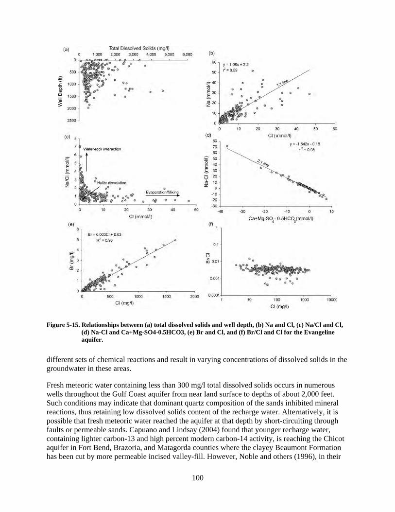
100

Figure 5-15. Relationships between (a) total dissolved solids and well depth, (b) Na and Cl, (c) Na/Cl and Cl, (d) Na-Cl and Ca+Mg-SO4-0.5HCO3, (e) Br and Cl, and (f) Br/Cl and Cl for the Evangeline aquifer.

different sets of chemical reactions and result in varying concentrations of dissolved solids in the groundwater in these areas.

Fresh meteoric water containing less than 300 mg/l total dissolved solids occurs in numerous wells throughout the Gulf Coast aquifer from near land surface to depths of about 2,000 feet. Such conditions may indicate that dominant quartz composition of the sands inhibited mineral reactions, thus retaining low dissolved solids content of the recharge water. Alternatively, it is possible that fresh meteoric water reached the aquifer at that depth by short-circuiting through faults or permeable sands. Capuano and Lindsay (2004) found that younger recharge water, containing lighter carbon-13 and high percent modern carbon-14 activity, is reaching the Chicot aquifer in Fort Bend, Brazoria, and Matagorda counties where the clayey Beaumont Formation has been cut by more permeable incised valley-fill. However, Noble and others (1996), in their

101

Figure 5-16. Relationships between (a) total dissolved solids and well depth, (b) Na and Cl, (c) Na/Cl and Cl, (d) Na-Cl and Ca+Mg-SO4-0.5HCO3, (e) Br and Cl, and (f) Br/Cl and Cl for the Jasper aquifer.

investigation on recharge over a small section of the Gulf Coast aquifer in Harris County, observed essentially no tritium at depths greater than 80 feet. Therefore, modern recharge was perhaps not reaching the aquifer beyond that depth in that area. Complex aquifer geometry, heterogeneity of sand bodies, interfingering of clays contained within the sands, and discontinuity of shale beds suggest that younger recharge water may reach to varying depths in the various parts of the Gulf Coast aquifer.

The increased salinity observed in groundwater along regional flow paths in Harris and Galveston counties is partly related to cation-exchange reactions in which sodium attached on clay minerals replaces calcium ions dissolved in groundwater. Modification of groundwater by cation exchange is a well documented process (Kreitler and others, 1977; Appello, 1994). This is supported by an inverse correlation between sodium and calcium (r2 = -0.66) and a positive

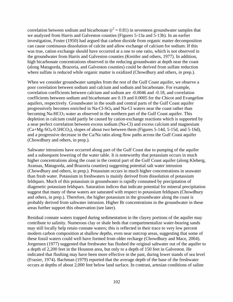
102

correlation between sodium and bicarbonate (r2 = 0.81) in seventeen groundwater samples that we analyzed from Harris and Galveston counties (Figures 5-13a and 5-13b). In an earlier investigation, Foster (1950) had argued that carbon dioxide from organic matter decomposition can cause continuous dissolution of calcite and allow exchange of calcium for sodium. If this was true, cation exchange should have occurred at a one to one ratio, which is not observed in the groundwater from Harris and Galveston counties (Kreitler and others, 1977). In addition, high bicarbonate concentrations observed in the reducing groundwater at depth near the coast (along Matagorda, Brazoria, and Galveston counties) could be derived from sulfate reduction where sulfate is reduced while organic matter is oxidized (Chowdhury and others, in prep.).

When we consider groundwater samples from the rest of the Gulf Coast aquifer, we observe a poor correlation between sodium and calcium and sodium and bicarbonate. For example, correlation coefficients between calcium and sodium are -0.0046 and -0.18, and correlation coefficients between sodium and bicarbonate are 0.19 and 0.0005 for the Chicot and Evangeline aquifers, respectively. Groundwater in the south and central parts of the Gulf Coast aquifer progressively becomes enriched in Na-Cl-SO4 and Na-Cl waters near the coast rather than becoming Na-HCO3 water as observed in the northern part of the Gulf Coast aquifer. This depletion in calcium could partly be caused by cation-exchange reactions which is supported by a near perfect correlation between excess sodium (Na-Cl) and excess calcium and magnesium (Ca+Mg-SO4-0.5HCO3), slopes of about two between them (Figures 5-14d, 5-15d, and 5-16d), and a progressive decrease in the Ca/Na ratio along flow paths across the Gulf Coast aquifer (Chowdhury and others, in prep.).

Saltwater intrusions have occurred along part of the Gulf Coast due to pumping of the aquifer and a subsequent lowering of the water table. It is noteworthy that potassium occurs in much higher concentrations along the coast in the central part of the Gulf Coast aquifer (along Kleberg, Aransas, Matagorda, and Brazoria counties) suggesting potential salt water intrusion (Chowdhury and others, in prep.). Potassium occurs in much higher concentrations in seawater than fresh water. Potassium in freshwaters is mainly derived from dissolution of potassium feldspars. Much of this potassium in groundwater is rapidly consumed by precipitation of diagenetic potassium feldspars. Saturation indices that indicate potential for mineral precipitation suggest that many of these waters are saturated with respect to potassium feldspars (Chowdhury and others, in prep.). Therefore, the higher potassium in the groundwater along the coast is probably derived from saltwater intrusion. Higher Br concentrations in the groundwater in these areas further support this observation (see later).

Residual connate waters trapped during sedimentation in the clayey portions of the aquifer may contribute to salinity. Numerous clay or shale beds that compartmentalize water-bearing sands may still locally help retain connate waters; this is reflected in their trace to very low percent modern carbon composition at shallow depths, even near outcrop areas, suggesting that some of these fossil waters could well have formed from older recharge (Chowdhury and Mace, 2004). Jorgensen (1977) suggested that freshwater has flushed the original saltwater out of the aquifer to a depth of 2,200 feet in the Houston area, but only to a depth of 150 feet in Galveston. He indicated that flushing may have been more effective in the past, during lower stands of sea level (Frazier, 1974). Bachman (1979) reported that the average depth of the base of the freshwater occurs at depths of about 2,000 feet below land surface. In contrast, artesian conditions of saline

103

aquifers underlying Duval County make the base of the saline water appear near land surface (Wood and others, 1963).

Trace Elements Trace elements generally occur in groundwater at concentrations of less than 1 mg/l. Like the major elements, trace elements in groundwater are derived from weathering of minerals and/or human activities. Trace element concentrations in groundwater largely depend on intensity of chemical weathering and their presence in minerals that are subjected to weathering (Drever, 1988). For example, many of the trace elements do not substitute readily in feldspar and other ferromagnesian minerals that are common sources of major elements but may be present in chemically resistant accessory minerals such as zircon, apatite, or zircon or as sulfides. In addition, burning of fossil fuels, smelting of ores, mining activities, and sewage disposal may introduce trace elements in groundwater (Drever, 1988).

Bromide and Iodide

The main source of chloride and bromide in groundwater is derived from atmospherically transported material that falls as wet precipitation and particulate matter (Davis and others, 1998). Near the coast this material is dominated by sea salt entrained in the air from the sea surface (Davis and others, 1998). Dry lake beds can contribute enough dust locally to overwhelm other sources of chloride and bromide (Wood and Sanford, 1995). Dissolution of evaporite and salt deposits, clay compaction, recrystallization of minerals, connate water, and saltwater intrusion may contribute additional bromide. Oil and gas activities, irrigation, and sewage disposal are some of the many human activities that can alter the natural concentrations of chloride (Cl-) and bromide (Br-). Ratios of bromide to chloride have been extensively used in the determination of sources of salinity. For example, these ratios have been successfully utilized to (1) make distinction between salinity originating from oil-field brine and salinity related to natural dissolution of halite, (2) identify mixing of brine derived from dissolution of halite and precipitation, (3) determine origin and fate of chloride in regional flow systems, and (4) assess effects of irrigation and sewage disposal on ambient chloride concentrations (Stevens, 1990; Fabryka-Martin and others, 1991; Whittemore, 1993).

Iodide behaves similar to bromide and chloride. These halides, along with their isotopes, are the most conservative constituents of groundwater and therefore may help in determining the origins of the water and subsurface geochemical processes (Fabryka-Martin and others, 1991). The presence of iodide is considered a good indicator of groundwater residence time, since more iodide leaches out of the sediments over time (Lloyd and others, 1982). Ratios of iodide to chloride have been effectively used to differentiate saltwater intrusion from fresh waters (Richter and Kreitler, 1991).

Methods We collected bromide and chloride concentration data for 2005 from the TWDB’s Groundwater Database. We plotted bromide/chloride ratios along with elevations of salt domes on a map to observe any association between them. We cross plotted both bromide and chloride and their

104

ratios against chloride to observe any trend that might exist between the two parameters, determine any potential mixing between various source waters, and identify sources of these ions.

Only a limited number of samples in the TWDB’s groundwater database have iodide values. We observed spatial distribution of iodide and evaluated any relationship that might exist between iodide concentrations and flow systems.

Results We analyzed bromide (Br-) concentrations from the Chicot, Evangeline, and Jasper aquifers (Tables 5-3 and 5-4). Concentrations of Br- range from 0.02 to 5.7 mg/l, 0.02 to 4.94 mg/l, and 0.02 to 4.04 mg/l in the Chicot, Evangeline, and Jasper aquifers, respectively. We observed a higher median value of bromide at shallower depths and a decrease in their concentrations with an increase in well depth (Table 5-3).

Table 5-3. Concentrations of bromide (Br-) in the Chicot, Evangeline, and Jasper aquifers.

Aquifer Range of Br concentration (mg/l) Median Br (mg/l) Standard deviation Number of analysesChicot aquiferEvangeline aquiferJasper aquifer

0.02 - 5.70.02 - 4.940.02 - 4.04

0.310.270.22

0.870.830.78

23925697

Table 5-4. Cl-/Br- ratios in the Chicot, Evangeline, and Jasper aquifers.

Aquifer Br/Cl (weight ratios)Range Mean Median Standard deviation Number of samples

ChicotEvangelineJasper

0.0051 - 0.0129 0.003254 0.00304 0.001585 2390.00004 - 0.01457 0.003413 0.003292 0.001398 2560.00072 - 0.10742 0.00534 0.003853 0.10688 97

Ratios of bromide to chloride have median values of 3.04×10-3, 3.29×10-3, and 3.85×10-3 in the Chicot, Evangeline, and Jasper aquifers, respectively (Table 5-4). Both mean and median ratios of bromide to chloride increase from the shallower to the deeper aquifers (Table 5-4). Ratios of bromide to chloride are most variable in the Jasper aquifer as indicated by their large standard deviations (Table 5-4). Plots of bromide versus chloride indicate correlation coefficients of 0.79, 0.93, and 0.95 for the Chicot, Evangeline, and Jasper aquifers, respectively (Figures 5-14e, 5-15e, and 5-16e). Plots of bromide to chloride ratio versus chloride show a general increase with an increase in chloride levels in a few wells (Figures 5-14f, 5-15f, and 5-16f). However, a large majority of the samples in the Chicot, Evangeline, and Jasper aquifers show a near constant bromide to chloride ratio with an increase in chloride concentration (Figures 5-14f, 5-15f, and 5-16f).

When we evaluated iodide concentrations, we observed that iodide exhibits poor correlation with chloride for the Chicot aquifer (r2 = 0.05, n = 17, where n is the number of samples) and a slightly better correlation for the Evangeline aquifer (r2 = 0.31, n = 20). Iodide and bromide similarly show a poor correlation for the Chicot aquifer (r2 = 0.07, n = 17) and a better correlation (r2 = 0.28, n = 20) for the Evangeline aquifer. Iodide is present in relatively small concentrations that range from 0.10 to 0.66 mg/l, with most samples containing less than 0.2 mg/l iodide.

105

Discussion

Concentrations of bromide and chloride in the Chicot, Evangeline, and the Jasper aquifers show good correlation coefficients suggesting a common source to the salinity (Figures 5-17 and 5-18). Salinity in the groundwater must be caused in part by dissolution of halite from salt domes that penetrate the aquifers at different stratigraphic intervals. This is supported by (1) low bromide and low bromide to chloride weight ratios (~10-4) in close proximity to salt domes particularly along Brazoria through Harris to Orange counties (Figures 5-17 and 5-18) and (2) molar Na/Cl ratios close to 1 in samples close to the salt domes, which would be expected if dissolution of halite was the source of this salinity. However, the effects of halite dissolution are not observed in groundwater across the aquifers, because the higher density of salt-laden groundwater near the domes causes groundwater to sink (Evans and others, 1991). Effects of

Figure 5-17. Distribution of Br/Cl molar ratios, location of salt domes, and top elevations of salt domes in the Gulf Coast aquifer in Texas (locations and elevations of salt domes after Hamlin, this volume).

106

Figure 5-18. Distribution of bromide concentrations in the Gulf Coast aquifer in Texas.

halite dissolution are more commonly observed in groundwater in close proximity to salt domes (Evans and others, 1991). Evans and others (1991) further contend that in salt dome environments groundwater is driven upward by density gradients that are associated with advective transport of dissolved salts and manifested in salinity plumes extending from the top of some salt domes.

When we considered Br/Cl ratios from across the Gulf Coast aquifer, we observed that most of the ratios are an order of magnitude higher than what would be expected if groundwater was mainly affected by halite-dissolution. For example, the median Br/Cl weight ratios are 3.04×10-3, 3.29×10-3, and 3.85×10-3 for the Chicot, Evangeline, and Jasper aquifers, respectively (Table 5-

107

4). Ratio of Br/Cl for seawater is about 3.3×10-3, which is close to connate formation water (Richter and Kreitler, 1991, Davis and others, 1998) and not significantly different from fresh waters (3.2×10-3 to 3.1×10-3; CB-DP, 2000). Therefore, the Br/Cl ratios suggest that a large number of groundwater samples are dominated by fresh meteoric recharge, with some contributions of residual connate water that escaped flushing during low stands of sea level, particularly in the central and the southern parts of the Gulf Coast aquifer. These groundwater samples have Na/Cl ratios close to 1, which suggests additional mixing of water derived from dissolution of halite and associated evaporites. We recognize that some of these ratios were affected by cation-exchange reactions. The relative importance of the cation-exchange reactions, halite-dissolution, and sea-water intrusion processes are discussed in greater detail elsewhere (Chowdhury and others, in prep.). Several samples along the coast (Kleberg, Nueces, Aransas, Matagorda and Brazoria counties) have higher concentrations of bromide that suggest modern saltwater intrusions have occurred (Figure 5-18).

Numerous groundwater samples across the Gulf Coast aquifer have bromide to chloride ratios that range from 4×10-3 to 1×10-1 (Figure 5-17). These ratios are typical of formation brines (Kreitler and Richter, 1986). Morton and others (1983) reported that bromide to chloride ratios in Tertiary brines of the underlying formations along the Texas Gulf Coast occur at less than 5×10-3 in the northern part, between 5×10-3 to 1×10-2 in the central and the southern part, and greater than 1×10-2 along a narrow band from Kleberg to Jackson counties (Morton and others, 1983). Occurrences of bromide to chloride ratios in groundwater similar to Tertiary brines in different areas of the Texas Gulf Coast aquifer may suggest that upward migration of formation brines may have locally altered their initial bromide to chloride ratios. Upward migration of deeper fluids to shallower depth has been proposed based on similar carbon isotope signatures in methane gas sampled from deep reservoirs and near land surface (Stahl and others, 1981). Others have postulated upward migration of deeper fluids to shallow depths along faults where uranium deposits were formed from mixing of reducing brine and oxidizing meteoric water (Galloway and others, 1982; Goldhaber and others, 1983; Kreitler and Richter, 1986). Therefore, salinity in groundwater in different parts of the Texas Gulf Coast aquifers could be derived from one or more sources, including halite dissolution, residual connate water trapped in the pore spaces during sedimentation, and upward migration of formation brines depending on the geographic area and local hydrogeologic conditions (Chowdhury and others, in prep.).

Slow diffusion of ions from fine-grained clay, silt, and sandstones may partly contribute chloride, bromide, and iodide (Fabryka-Martin and others, 1991). Slow diffusion of bromide and chloride from interstitial water may be facilitated as groundwater movement is hindered through the subsurface by the complex geometry of the aquifer materials and the abundance of fine-grained clays. In the Milk River Formation of Alberta, Fabryka-Martin and others (1991) showed that high concentrations of iodide and bromide in the groundwater down hydraulic gradients are related to organic matter diagenesis. They observed that both bromide and chloride concentrations increase down hydraulic gradients and that chloride, iodide, and bromide show near perfect correlations between them. In the Gulf Coast aquifer, from the limited data on iodide available, we note that iodide is present at less than 0.2 mg/l in most of the analyzed samples. Correlation coefficients between chloride and iodide and iodide and bromide are considerably low (r2 = 0.06 and 0.07, respectively, for the Chicot aquifer and r2 = 0.31 and 0.28, respectively, for the Evangeline aquifer). Moreover, neither iodide nor bromide shows any preferential enrichment along regional flow paths. Therefore, while it is possible that some bromide,

108

chloride, and iodide could be derived from shale contained in the sandstones and shale beds, their contribution, if any, is likely to be small. Additional information on iodide and chloride isotopes may further assist identifying sources of these halogens.

Arsenic

Arsenic (As) is introduced in water through dissolution of minerals and ores. Arsenic concentrations in groundwater increase as a result of erosion of local rocks containing iron oxides, iron sulfides, and from geothermal sources (WHO, 2001, Smedley and Kinniburgh, 2002; Scanlon and others, 2005). Anthropogenic sources such as industrial effluents, alloying agents, wood preservatives, defoliants, herbicides, insecticides, and combustion of fossil fuels also contribute arsenic to atmospheric deposition (Stollenwerk, 2003; Scanlon and others, 2005)Inorganic arsenic can occur in several forms, but it commonly occurs as trivalent arsenite (As[III]) or pentavalent arsenate (As[V]) in natural waters. Arsenic is a human health concern because it can contribute to skin, bladder, and other cancers (NRC, 1999).

Methods

We collected all available arsenic data on the Gulf Coast aquifer from TWDB’s groundwater database for 1995. However, as only a few samples were collected in 1995 for the Catahoula Formation, we included arsenic data for 1986 to 2005 to provide a better spatial distribution. Wanalyzed spatial distribution of arsenic in the Gulf Coast aquifer. We plotted several element parameters versus arsenic in order to identify sources of arsenic in the groundwater. We evaluated arsenic concentrations in light of oxidizing-reducing potential of a limited number of groundwater samples from the Evangeline aquifer.

Results

We analyzed arsenic concentrations in the groundwater from the Chicot, Evangeline, and Jasperaquifers (Table 5-5). We observed that arsenic concentrations range from 2 to 26.8 micrograms per liter (µg/l), 2.03 to 75 µg/l, and 2 to 569 µg/l in the Chicot, Evangeline, and the Jasper aquifers, respectively (Table 5-5). About 7.5, 11.5, and 30 percent of groundwater samples fromthe Chicot, Evangeline, and Jasper aquifers, respectively, have more than 10 µg/l arsenic, the recommended limit for drinking water purposes (U.S. EPA, 2001). The highest concentrations oarsenic occur in the Jasper aquifer. Samples with high concentrations of arsenic commonly occuin the southwestern part of the Evangeline and the Jasper aquifers in the areas of Duval, Webb, Live Oak, Karnes, and Jim Wells counties (Figures 5-19, 5-20 and 5-21). We observed no preferential occurrence of arsenic with depth and no significant relationship at depth with molybdenum or manganese (Figures 5-22a, 5-22c, and 5-22g). On bivariate plots, arsenic and

.

f r

e

Table 5-5. Arsenic concentrations in the Chicot, Evangeline, and Jasper aquifers.

Aquifer Concentrations of arsenic (As) (µg/l)Range of arsenic concentration Mean Median Percent exceedance Standar

4.2210.1743.40

319355295

d deviation Number of samplesChicotEvangelineJasper

2 - 26.82.03 - 75

2 - 569

3.858.0318.85

2.044.74

5

7.511.54

30

109

Figure 5-19. Distribution of arsenic concentrations in the Chicot aquifer.

vanadium show strong correlation coefficients (r2 = 0.74; Figure 5-22b), but poor correlations were observed between arsenic and manganese (r2 = 0.05; Figure 5-22c) and arsenic and molybdenum (r2 = 0.04; Figure 5-22g). Arsenic is also poorly correlated with sulfate (r2 = 0.03; Figure 5-22d), chloride (r2 = 0.22; Figure 5-22e), and Br/Cl ratios (r2 = 0.02; Figure 5-22f). Comparison of arsenic concentrations with oxidation-reduction potential of a few samples from the Evangeline aquifer suggest that arsenic concentrations decline slightly under highly reducing (<-300 mV) and oxidizing conditions (>+250 mV; Figure 5-22h). At slightly-oxidizing to slightly-reducing conditions, maximum concentrations of arsenic were observed (Figure 5-22h).

Discussion

Arsenic, molybdenum, selenium, and vanadium in the Gulf Coast aquifer could be derived from weathering of interstratified volcaniclastic debris derived from Sierra Madre Occidental of Mexico and the Trans-Pecos Region of West Texas (Galloway and others, 1982). Smedley and

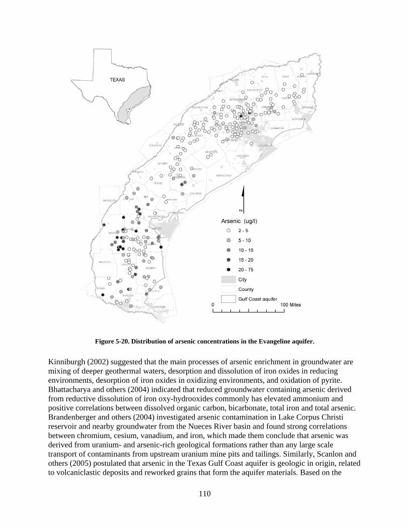
110

Figure 5-20. Distribution of arsenic concentrations in the Evangeline aquifer.

Kinniburgh (2002) suggested that the main processes of arsenic enrichment in groundwater are mixing of deeper geothermal waters, desorption and dissolution of iron oxides in reducing environments, desorption of iron oxides in oxidizing environments, and oxidation of pyrite. Bhattacharya and others (2004) indicated that reduced groundwater containing arsenic derived from reductive dissolution of iron oxy-hydrooxides commonly has elevated ammonium and positive correlations between dissolved organic carbon, bicarbonate, total iron and total arsenic. Brandenberger and others (2004) investigated arsenic contamination in Lake Corpus Christi reservoir and nearby groundwater from the Nueces River basin and found strong correlations between chromium, cesium, vanadium, and iron, which made them conclude that arsenic was derived from uranium- and arsenic-rich geological formations rather than any large scale transport of contaminants from upstream uranium mine pits and tailings. Similarly, Scanlon and others (2005) postulated that arsenic in the Texas Gulf Coast aquifer is geologic in origin, related to volcaniclastic deposits and reworked grains that form the aquifer materials. Based on the

111

Figure 5-21. Distribution of arsenic concentrations in the Jasper aquifer. Note color codes refer to higher values than the Chicot and the Evangeline aquifers due to higher concentrations of arsenic in the Jasper aquifer.

results from unsaturated zone studies, Scanlon and others (2005) suggested that cotton production in the southern part of the Gulf Coast aquifer was probably not responsible for arsenic pollution of the groundwater except locally.

We observed that arsenic concentrations become enriched at depth, progressing from the Chicot to the Evangeline and to the Jasper aquifers (Table 5-5).There is a large degree of variability in arsenic concentrations within each aquifer, as evident from their significant standard deviations (Table 5-5). For example, in the Goliad Sand and the Catahoula Formation, arsenic occurs at random with depth and shows a wide scatter in concentrations. This irregularity in arsenic occurrence may partly be attributed to the depositional facies with finer-grained materials containing more arsenic. Brandenberger and others (2004) suggested that arsenic enrichment in

112

Figure 5-22. Relationships in the Evangeline aquifer between: (a) arsenic concentration and well depth, (b) concentrations of arsenic and vanadium, (c) concentrations of arsenic and manganese, (d) concentrations of arsenic and sulfate, (e) concentrations of arsenic and chloride, (f) Br/Cl weight ratios and arsenic concentrations, (g) concentrations of arsenic and molybdenum, and (h) arsenic concentrations and oxidation-reduction potential.

113

the groundwater and the surface water in the Nueces River Basin is caused by iron-rich detrital clay minerals and not reactive iron oxy-hydroxides.We observed a spatial bias to the occurrence of higher concentrations of arsenic in south Texas (in Duval, Webb, Live Oak, Karnes, and Jim Wells counties) following the outcrop of the Jasper aquifer (Oakville and Catahoula formations) that host most of the uranium deposits (Figures 5-20 and 5-21). Therefore, in addition to the reworked volcanoclastic materials, arsenic may source from dissolution of arsenic-rich sulfides and/or desorption of iron oxides present in uranium deposits. These sulfide-rich waters may flow upward to move dissolved arsenic farther from the source in the Catahoula Formation to the Evangeline and the Chicot aquifers. Reductive dissolution of iron hydroxides may cause development of arsenic in the reducing parts of the aquifer.

Low concentrations of dissolved iron and manganese in the groundwater suggest that most of these waters are probably under slightly reducing to slightly oxidizing conditions. For example, dissolved median values of iron concentrations in the Chicot and the Evangeline aquifers are about 0.1 mg/l (n = 1,700). Similarly, dissolved median values of manganese concentrations in the Chicot and the Evangeline aquifers are about 0.01 mg/l (n = 442) and 0.02 mg/l (n = 622), respectively. Henry and others (1982) used Eh measurements to illustrate that groundwater is under oxidizing conditions near the outcrop and progressively becomes more reducing down flow paths in the Oakville sand. We observed a poor correlation between arsenic and molybdenum (r2 = 0.04) and arsenic and manganese (r2 = 0.05) and a strong correlation between arsenic and vanadium (r2 = 0.74) (Figures 5-22b, 5-22c, and 5-22g). A strong association between arsenic and vanadium indicate their derivation from similar mineral sources, probably from desorption under high pH conditions (Lee and Herbert, 2002; Smedley and Kinniburgh, 2002). Poor correlations between arsenic and sulfate (r2 = 0.03) (Figure 5-22d), arsenic and chloride (r2 = 0.22) (Figure 5-22e), and arsenic and Br/Cl ratios (r2 = 0.02) (Figure 5-22f) suggest that arsenic was less likely to have directly derived from the upwelling of deeper formation brines. Additional data on redox and nutrient conditions in the groundwater is required to further constrain processes responsible for mobilization of arsenic (Chowdhury and others, in prep.).

Comparison of oxidation-reduction potential to arsenic concentrations in several groundwater samples from the Evangeline aquifer indicate that arsenic concentration is higher in slightly-reducing to slightly-oxidizing (-100 to +100 mV) conditions, perhaps due to preferential dissolution of iron sulfides and iron oxides in this environment (Figure 5-22h). A decrease in arsenic concentrations under highly oxidizing and highly reducing conditions could probably be attributed to arsenic co-precipitation and adsorption by interaction with Fe- and Mn-oxides, as well as precipitation of sulfidic minerals containing co-precipitated arsenic in these environments (Smedley and Kinniburgh, 2002).

Radioactivity

High levels of radioactivity in drinking water are a potential carcinogen to humans (Cech and others, 1987b; Hudak, 2005). An association between radioactivity in groundwater and cancer has been documented in numerous epidemiological studies (Lyman and others, 1985). Radium-226 and radon-222, products of the uranium-238 decay series, are the precursors to radioactivity observed in groundwater samples. Radium-226 has a half-life of 1,602 years and radium-228 has a half-life of 5.7 years (Cech and others, 1987a). Radon-222 has a half-life of 3.82 days.

114

Sediments formed under reducing conditions generally contain high levels of trace metals, including uranium and thorium (Langmuir, 1997). The U.S. Environmental Protection Agency recommends maximum contaminant levels (MCL) of 15 picocuries per liter (pCi/l) for alpha activity or 50 pCi/l for beta activity (U.S. EPA, 1976).

Methods

We collected all available radioactivity data on the Gulf Coast aquifer from TWDB’s Groundwater Database. We analyzed spatial distributions of radioactivity in the Gulf Coast aquifer. We plotted alpha versus beta activities to observe whether any genetic relationship exists between them. We also evaluated radium-225 and radon concentrations on a few samples.

Results

We analyzed radioactivity levels in samples from the Chicot, Evangeline, and Jasper aquifers (Figures 5-20, 5-21, and 5-22). Groundwater from the Evangeline aquifer in Harris County and groundwater from the Evangeline aquifer in areas south of Bee County have high concentrations of alpha activity relative to the rest of the aquifer system. Radioactivity generally increases from the northern part to the southern part of the Gulf Coast aquifer (Figures 5-23, 5-24, and 5-25). Radioactivity occurs irregularly with depth and shows no trend in composition (Figures 5-26a, 5-26c, and 5-26e). Radioactivity in the TWDB’s Groundwater Database is mainly expressed as gross-alpha and gross-beta. A small portion of the samples that we examined exceed in alpha activity (Table 5-6). Only about one percent of samples from the Chicot aquifer, six percent of samples from the Evangeline aquifer, and three percent of samples from the Jasper aquifer have more than the MCL for alpha activity (Table 5-6). Nearly all samples that we analyzed are below the MCL for beta activity (Table 5-7). We observed low positive correlations between alpha and beta activities (r2 = 0.47, r2 = 0.05, and r2 = 0.55 for the Chicot, Evangeline, and Jasper aquifers, respectively; Figures 5-26d, 5-26e, and 5-26f). About a dozen samples have radium-226 and radon-222 concentrations and corresponding alpha activity in the TWDB’s Groundwater Database for the Gulf Coast aquifer. We found that radium-226 concentrations range from 0.6 to 2.1 pCi/l. Radon-222 concentrations range from 101 to 203 pCi/l with 2 to 21 µg/l of uranium-238. We observed only a low positive correlation between radon-222 and alpha activity (Figure 5-26g).

Discussion

Several authors have sought to determine the origin of high concentrations of radium-226 in groundwater from the Gulf Coast aquifer of Texas (Kraemer and Reid, 1984; Cech and others, 1987b; Hudak, 2005). They reported that high concentrations of radium in groundwater from the Gulf Coast aquifer could probably be related to uranium occurrences in the aquifer materials (Cech and others, 1987b). In deeper formation brines of the Texas Gulf Coast, the presence of higher concentrations of radium-226 was attributed to formation water and mineral matrix reactions and preferential retention of radium-226 ions in solution; at higher salinity, the abundant positive ions compete with radium ions for adsorption sites (Tanner, 1964; Kraemer and Reid, 1984).

Cech and others (1987a) observed up to 22.5 pCi/l of radium-226 in groundwater in Harris County. They found high concentrations of radium-226 near salt domes, especially in wells located at depths between 180 to 350 meters. Due to limited data (n = 7), we were unable to

115

Figure 5-23. Distribution of alpha activity in the Chicot aquifer.

evaluate any relationship that might exist between radium-226 and alpha activity. Radium-226 concentrations in the analyzed groundwater are small and range from 0.1 to 0.6 pCi/l. Radon-22and alpha activity show moderate correlation (r2 = 0.42; Figure 5-26g). A small portion of the samples that we examined exceed the MCL of alpha activity (Table 5-6). Only about one percenof samples from the Chicot aquifer, six percent of samples from the Evangeline aquifer, and three percent of samples from the Jasper aquifer have alpha activity that exceeds the MCL (Tabl5-6). No preferential enrichment in alpha activity with depth was noted in the Chicot, Evangeline, or Jasper aquifers. However, there appears to be a spatial bias, with higher alpha activity in the southern and central parts than in the northern part of the Gulf Coast aquifer. Thisenrichment in higher alpha activity may likely be related to higher concentrations of uranium deposits, relative abundance of volcaniclastics in the aquifer materials, and wider influx of formation brines in the area.

2

t

e

116

Figure 5-24. Distribution of alpha activity in the Evangeline aquifer.

Most of the groundwater analyzed from the Chicot, Evangeline, and Jasper aquifers has low beta activity (Table 5-7). Beta activity is moderately to poorly correlated to alpha activity in the Chicot (r2 = 0.47), Evangeline (r2 = 0.05), and Jasper aquifers (r2 = 0.55; Figures 5-23b, 5-23d, and 5-23e). Primary sources of beta activity in groundwater include radiation from 40K and 228Ra (Welch and others, 1995). Ingrowth of beta-emitting radionuclide can contribute to gross-beta activity during sample holding times, particularly in groundwater exceeding gross-beta activities of 10 pCi/L (Welch and others, 1995). It is believed that both alpha and beta activities are sourced from parent uranium activity in groundwater (Hudak, 2005). Therefore, both these parameters should be well correlated. However, we observe that some samples containing the highest concentrations of alpha activity have the lowest concentrations of beta activity (Table 5-7; Figures 5-26d, 5-26e, and 5-26f). Additional information is needed to better constrain the sources of alpha and beta activity. The radioactivity in the groundwater is discussed in more detail in Chowdhury and others (in prep.).

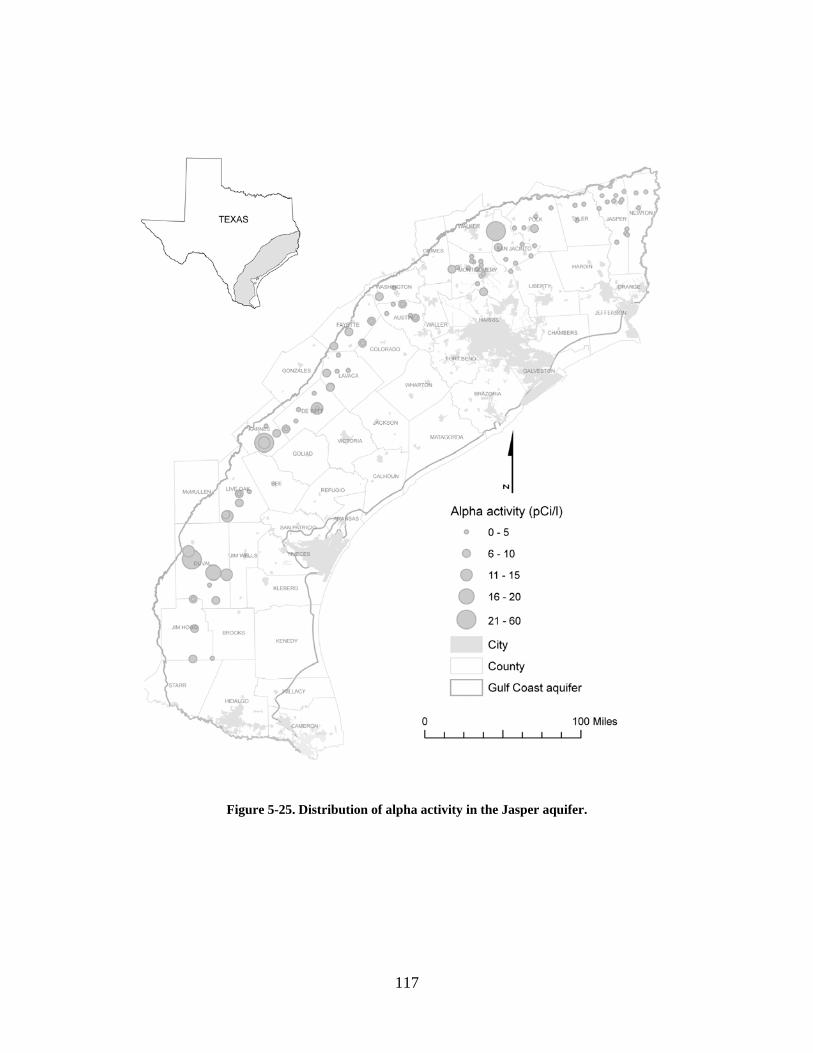
117

Figure 5-25. Distribution of alpha activity in the Jasper aquifer.

118

Figure 5-26. Relationships between alpha activity and well depth in the (a) Chicot aquifer, (b) Evangeline aquifer, and (c) Jasper aquifer; relationships between alpha versus beta activities in the (d) Chicot aquifer, (e) Evangeline aquifer, and (f) Jasper aquifer; and (g) relationship between alpha and radon-222 activities in the Evangeline aquifer.

119

Table 5-6. Alpha activity in the Chicot, Evangeline, and Jasper aquifers.

AquiferMinimum Maximum Mean Median Percent exceedance Number of samples

Chicot aquifer 0 60 2.90 1.90 1.03 289Evangeline aquifer 0 208 6.05 2.60 6.27 272Jasper aquifer 0.20 39 4.45 2.65 3.41 117

Alpha activity (pCi/l)

Table 5-7. Beta activity in the Chicot, Evangeline, and Jasper aquifers.

AquiferMinimum Maximum Mean Median Percent exceedance Number of samples

Chicot aquifer 0.00 80.00 4.96 3.60 0.34 289Evangeline aquifer 0.60 33.00 6.72 4.65 0.00 272Jasper aquifer 1.20 43.00 9.39 7.70 0.00 117

Beta activity (pCi/l)

Relationships between Water-level Decline and Groundwater Composition Groundwater composition in interbedded sand and shale aquifers are commonly affected by decline in water levels in wells. Initial pumping removes water from the sandier portions of the aquifer that are readily removed due to higher hydraulic conductivity of the aquifer materials. Continued pumping removes water from the more finer-grained clay beds that commonly host more saline water. Under natural conditions, recharge to and discharge from an aquifer are in equilibrium (Theis, 1940). In order to maintain a dynamic equilibrium in an aquifer, recharge must equal to discharge. With continued groundwater pumping, natural discharge areas may decrease, recharge areas may increase, and/or aquifer storage may decline.

Water levels in the Gulf Coast aquifer have declined by several hundred feet due to groundwater pumping (Chowdhury and others, 2004; Kasmarek and Robinson, 2004). Water-level decline causes expulsion of water from interbedded clays due to compaction and rearrangement of the clays (Kasmarek and Robinson, 2004). Continued water-level decline may result in subsidence of the land surface.

Methods

We developed hydrographs for selected wells using historical information from various parts of the Gulf Coast aquifer in areas with large drawdown and/or land-surface subsidence (Harris and Wharton counties) to document effects of water-level decline on groundwater composition. To investigate the possible relationship between groundwater compositions and water-level decline, we plotted TDS, Na, Cl, HCO3, and specific conductance values with water-level decline. Relationships between groundwater composition and water-level decline as observed in three wells are presented below.

Results

We selected a few wells from areas where water levels have declined historically and caused land-surface subsidence (Figures 5-27a, 5-27b, and 5-27c). We compared changes in

120

Figure 5-27. Changes in groundwater composition with water-level declines during the historical record from selected wells in Harris and Wharton counties.

121

groundwater composition in some of these wells with water-level declines through time. We observed that groundwater composition does not appear to significantly change with water-level declines (Figures 5-24b and 5-24c). In some cases, a slight but gradual increase in salinity was observed (Figure 5-24a). However, in a few shallow wells, water-level decline is associated with a freshening of the aquifer probably due to changes in the hydraulic regime that captures fresher water from the outcrop.

Discussion

Groundwater quality commonly deteriorates with residence time in the aquifer. Therefore, in the presence of unstable minerals in the aquifer, progressive water-rock interaction makes groundwater more saline. Clays and shale beds contained within the aquifer are inefficient to flush out connate water due to their low effective porosities. In the northern part of the Gulf Coast aquifer in Texas, excessive groundwater pumping leads to clay compaction that causes expulsion of water contained within the pore spaces of the clays (Kasmarek and Robinson, 2004). More than 25 percent of the groundwater in the northern part of the Gulf Coast aquifer is believed to have been derived from clay compaction (Jorgensen, 1975; Kasmarek and Robinson, 2004). We attempted to evaluate to what extent groundwater becomes saline due to water-level decline in wells.

In several wells, we observed that there are no significant changes in groundwater composition, even though water levels declined by hundreds of feet (Figure 5-27b). Composition may not change because water that is expelled due to clay compaction occurs through slow diffusive processes, as compaction and subsidence is small over time. For example, Gabrysch (1984) noted that land-surface subsidence was 0.5 feet from 1964 to 1973. Therefore, a small volume of water that is expelled from the clays mixes and become diluted in the larger freshwater reservoir in the aquifer. However, in some wells this deterioration in groundwater composition is more pronounced where the groundwater becomes more saline with progressive water-level decline (Figure 5-27a). This increase in salinity could occur if there is no significant mixing of the water expelled from the clays or if the clays had relatively fresher connate water. Jorgensen (1977) analyzed groundwater composition from clays at depths of 2 to 24 feet from Harris County. He found that groundwater composition is highly variable, generally increases in salinity with depth, and has specific conductance values that range from 586 to 2,120 micro-mhos (µmhos). In some wells that we analyzed, we note a freshening of the groundwater with water-level decline, possibly because pumping alters the natural hydraulic gradient and captures more fresh water from the outcrop. Relationships between water-level decline and changes in groundwater composition are discussed in more detail elsewhere (Chowdhury and others in prep.).

Conclusions Fresh meteoric water containing less than 300 mg/l total dissolved solids occurs in numerous wells throughout the Gulf Coast aquifer in Texas from near land surface to depths of about 2,000 feet. Sandstone compositions in the northern part of the Gulf Coast are more commonly quartz arenite while to the south, sandstone compositions are more likely arkosic and greywackes containing abundant feldspar and rock fragments. A dominant quartz composition of the aquifer materials may have inhibited mineral reactions, thus retaining low dissolved solids content of the

122

recharge water. Groundwater in the central and southern parts of the Gulf Coast aquifer contains significantly more chloride, sulfate, and sodium than in the northern part of the Gulf Coast aquifer. These differences in composition from north to south are related to varying lithologies, rainfall levels, evaporation rates, and mineral reactions across the Gulf Coast aquifer. Cation exchange that removes dissolved calcium from the water and replaces it with sodium ions adsorbed on clay surfaces is a dominant process. This is supported from a gradual decrease in Ca/Na ratio along flow paths from the outcrop towards the coast.

Local enrichment in groundwater salinity around salt domes was probably caused by dissolution of halite that penetrates the aquifers at different stratigraphic intervals. This is supported by (1) low bromide and low bromide to chloride weight ratios (~10-4) in close proximity to salt domes, particularly in Brazoria, Harris, and Orange counties and (2) molar Na/Cl ratios close to 1 in samples close to the salt domes, as would be expected if dissolution of halite was the source of this salinity. When we considered Br/Cl ratios from across the Gulf Coast aquifer in Texas, we observed that most of the ratios are an order of magnitude higher than what would otherwise be expected if groundwater was mainly affected by halite dissolution. These ratios are more typical of seawater or connate formation water. Therefore, these Br/Cl ratios may suggest that some of this groundwater is a mixture of fresh meteoric water and connate formation water that escaped flushing during low sea-level stands, particularly in the central and the southern parts of the Gulf Coast aquifer. Some of this water has very low modern carbon activity indicating their origin from older recharge events. Local saltwater intrusion has occurred along the coast in Kleberg, Aransas, Matagorda, and Brazoria counties as indicated by higher bromide and potassium concentrations in these areas.

We observed that arsenic concentrations become enriched in progressing from the Chicot to the Evangeline to the Jasper aquifers. More arsenic occurs in proximity to the uranium deposits contained in the Catahoula Formation. Therefore, arsenic occurrence appears to be related to possible dissolution of sulfides and/or desorption of iron oxides from uranium deposits and their transport upwards into the Evangeline and the Chicot aquifers. However, arsenic is spatially distributed at random suggesting a possible role of iron oxides and sulfides available locally in the aquifer materials. Poor correlations between arsenic and Br/Cl ratios, chloride, and sulfate suggest that arsenic was less likely to have been directly derived from upwelling of deeper saline fluids. Comparison of oxidation-reduction potential with arsenic concentrations in several groundwater samples from the Evangeline aquifer indicate that arsenic mobilization is highest under slightly-reducing to slightly-oxidizing conditions, perhaps due to preferential dissolution of iron sulfides and iron oxides in this environment.

A small portion of the samples that we examined exceed maximum contaminant levels in alpha activity. Only about one percent of samples from the Chicot aquifer, six percent of samples from the Evangeline aquifer, and three percent of samples from the Jasper aquifer exceed maximum contaminant levels for alpha activity. We did not note preferential enrichment in alpha activity with depth in the Chicot, Evangeline, or Jasper aquifers. However, there appears to be a spatial bias with higher alpha activity in the southern and central parts than in the northern part of the Gulf Coast aquifer. Higher alpha activity may be associated with higher concentrations of uranium, relative abundance of volcaniclastics in the aquifer materials, and wider influx of deeper formation brines in the area. Most of the groundwater analyzed from the Chicot, Evangeline, and Jasper aquifers has low beta activity.

123

Groundwater composition may or may not change with water-level decline, depending on local hydrogeologic conditions. In several wells, we observed no significant changes in groundwater composition, even though water levels declined by hundreds of feet. This may be due to expulsion of connate water from the clays through diffusion and subsequent mixing and dilution with the larger freshwater reservoir in the aquifer. In a few wells, groundwater becomes more saline with water-level decline. This increase in salinity could occur due to an absence of mixing of the connate water with the fresher water in the aquifer. Other wells show a freshening of the aquifer with water-level decline, possibly because pumping alters the natural flow system, capturing more fresh water from the outcrop.

References Appello, C. A. J., 1994, Cation and proton exchange, pH variations, and carbonate reactions in a

freshening aquifer: Water Resources Research, v. 30, p. 2795–2805.

Bachman, A. L., 1979, Subsurface disposal of geopressured fluids—Potential geologic and operational problems with recommendations for disposal system testing, in Dorfman, M. H., and Fisher, W. L., Proceedings, 4th U.S. Gulf Coast geopressured-geothermal energy conference—Research and development: The University of Texas at Austin, Center for Energy Studies, v. 2, p. 972–999.

Baker, E. T., Jr., 1979, Stratigraphic and hydrogeologic framework of part of the coastal plain of Texas: Texas Department of Water Resources Report 236, 43 p.

Beckman, J. D., and Williamson, A. K., 1990, Salt-dome locations in the Gulf Coastal Plain, south-central United States: U. S. Geological Survey Water Resources Investigations Report 90-4060, 19 p.

Bhattacharya, P., Jacks, G., Valero, A., Tandukar, N., and Mukherjee, A., 2004, Mobilization of arsenic from the alluvial aquifers in Terai region of Nepal, in Sing, V. P., and Yadava, R. N., editors, Groundwater pollution: Bhopal, India, p. 303–312.

Brandenberger, J., Louchouran, P., Herbert, P., and Tissot, P., 2004, Geochemical and hydrodynamic controls on arsenic and trace metal cycling in seasonally stratified US sub-tropical reservoir: Applied Geochemistry, v. 19, p. 1601–1623.

Capuano, R. M, and Lindsay, S. V., 2004, Chicot/Evangeline aquifers of the Texas Gulf Coast, groundwater age and pathways for salt water contamination: Environmental Institute of Houston, 2004 Annual Report, 4 p.

Cartwright, I., Weaver, T. R., Fulton, S., Nichol, C., Reid, M., and Cheng, X., 2004, Hydrogeochemical and isotopic constraints on the origins of dryland salinity, Murray Basin, Victoria, Australia, Applied Geochemistry, v. 19, p. 1233-1254.

CB-DP, 2000, Water Quality Program Plan: Calfed Bay-Delta Program, p. 3-40–3-48.

Cech, I., Lemma, M., Prichard, H. M., and Kreitler, C. W., 1987a, Radium-226 and radon-222 in domestic water of Houston-Harris County, Texas in Graves, B., editor, Radon, radium, and other radioactivity in groundwater—Hydrogeologic impact and application to indoor airborne contamination: Chelsea, Michigan, Lewis Publishers, 546 p.

124

Cech, I. M., Howard, M. P., Mayerson, A., and Lemma, M., 1987b, Pattern of distribution of Radium 226 in drinking water of Texas: Water Resources Research, v. 23, p. 1987–1995.

Chowdhury, A. H, Bogichi, R., and Hopkins, J., in preparation, Hydrogeology, hydrochemistry, and trace constituents, Texas Gulf Coast aquifer: Texas Water Development Board Report.

Chowdhury, A. H., and Mace, R. E., 2004, Geochemical evolution of the groundwater in the Gulf Coast aquifer of South Texas, in Proceedings of groundwater flow understanding from local to the regional scales, XXXIII Congress International Association of Hydrogeologists and 7th Asociación Latinoamericana de Hidrologia Subterránea para el Desarrollo, Zacatecas City, Mexico, 4 p., CD-ROM, ISBN: 970-32-149-4.

Chowdhury, A. H., Wade, S., Mace, R., and Ridgeway, C., 2004, Groundwater availability model of the central Gulf Coast Aquifer System—Numerical simulations through 1999: Texas Water Development Board Report, 162 p.

Davis, S. N., Whittemore, D. O., and Fabryka-Martin, J., 1998, Uses of chloride/bromide ratios in studies of potable water: Groundwater, v. 36, no. 2, p. 338–350.

Drever, J. I., 1988, The geochemistry of natural waters: Englewood Cliffs, New Jersey, Prentice Hall, 437 p.

Evans, D. G., Nunn, J. A., and Hanor, J. S., 1991, Mechanisms driving groundwater flow near salt domes: Geophysical Research Letters, v. 18, no. 5, p. 927–930.

Fabryka-Martin, J., Whittemore, D. O., Davis, S. N., Kubik, P. O., and Sharma, P., 1991, Geochemistry of halogens in the Milk River aquifer, Alberta, Canada: Applied Geochemistry, v. 6, p. 447–464.

Foster, M. D., 1950, The origin of high sodium bicarbonate waters in the Atlantic and Gulf Coastal Plains: Geochimica et Cosmochimica Acta, v. 1, p. 33–48.

Frazier, D. E., 1974, Depositional episodes—Their relationship to stratigraphic framework in the northwestern portion of the Gulf Basin: University of Texas at Austin, Bureau of Economic Geology Circular 74–1, 28 p.

Gabrysch, R. K, 1984, Case history no. 9.12—The Houston-Galveston region, Texas, USA, in Poland, J. F., editor, Guidebook to studies of land subsidence due to groundwater withdrawal: UNESCO Studies and Reports in Hydrology, v. 20, p. 253–262.

Gabrysch, R. K. and Bonnet, C. W., 1975, Land-surface subsidence in the Houston-Galveston region, Texas: Texas Water Development Board Report 188, 19 p.

Galloway, W. E., 1982, Epigenetic zonation and fluid flow history of uranium-bearing fluvial aquifer systems, south Texas uranium province: The University of Texas at Austin, Bureau of Economic Geology Report of Investigations 119, 79 p.

Galloway, W. E., Hobday, D. K., and Magara, K., 1982, Frio Formation of the Texas Gulf Coast Basin—Depositional systems, structural framework, and hydrocarbon origin, migration, distribution and exploration potential: The University of Texas at Austin, Bureau of Economic Geology Report of Investigations 122, 78 p.

125

Goldhaber, M. B., Reynolds, R. L., and Rye, R. O., 1983, Role of fluid mixing and fault related sulfide in the origin of the Ray Point Uranium District, South Texas: Economic Geology, v. 78, p. 1043–1063.

Hamlin, S., this volume, Salt domes in the Gulf Coast aquifer: Texas Water Development Board Report 365, p. 217–230.

Harris-Galveston Coastal Subsidence District, 1998, Groundwater management plan: Friendswood, Texas, 72 p.

Henry, C. D., Galloway, W. E., Smith, G. E., Ho, C. L., Morton, J. P., and Gluck, J. K., 1982, Geochemistry of groundwater in the Miocene Oakville sandstone—A major aquifer and uranium host of the Texas Coastal Plain: The University of Texas at Austin, Bureau of Economic Geology Report of Investigations No. 118, 63 p.

Herczeg, A. L., and Edmunds, W. M., 2000, Inorganic ions as tracers, in Cook, P. G., and Herczeg, A. L., editors, Environmental tracers in subsurface hydrology: Boston, Massachusetts, Kluwer Academic Press, p. 31–79.

Hoel, H. D., 1982, Goliad Formation of the south Texas Gulf Coastal Plain—Regional genetic stratigraphy and uranium mineralization: The University of Texas at Austin, Masters’ thesis, 173 p.

Hudak, P. F., 2005, Radioactivity in the Ogallala and Dockum aquifers, northwest Texas: Environmental Geology, v. 47, p. 283–289.

Jorgensen, D. G., 1975, Analog model studies of groundwater hydrology in the Houston district, Texas, Texas Water Development Board Report 190, 84 p.

Jorgensen, D. G., 1977, Salt-water encroachment in aquifers near the Houston Ship Channel, Texas: U. S. Geological Survey Open File Report 76-781, 45 p.

Kasmarek, M. C., and Robinson, J. L., 2004, Hydrogeology and simulation of groundwater flow and land-surface subsidence in the northern part of the Gulf Coast aquifer system, Texas: U.S. Geological Survey Scientific Investigations Report 2004-1502, 111 p.

Kraemer, T. F., and Reid, D. F., 1984, The occurrence and behavior of radium in saline formation water of the US Gulf Coast region: Isotope Geoscience, v. 2, p. 153–174.

Kreitler, C. W., Guevara, E., Granata, G., McKalips, D., 1977, Hydrogeology of Gulf Coast aquifers, Houston-Galveston area, Texas: Transactions Gulf Coast Association of Geological Societies, v. 27, p. 72–89.

Kreitler, C. W., and Richter, B. C., 1986, Hydrochemical characterization of saline aquifers of the Texas Gulf Coast used for disposal of industrial waste: Prepared for the U.S. Environmental Protection Agency, Contract No. R-812785-01-0, The University of Texas at Austin, Bureau of Economic Geology, 114 p.

Langmuir, D., 1997, Aqueous environmental chemistry: Prentice-Hall, Englewood Cliffs, New Jersey, 600 p.

Lee, L., and Herbert, B. E., 2002, Arsenic and associated trace metals in Texas groundwater: American Geophysical Union Fall National Meeting, San Francisco, California.

126

Lindquist, S. J., 1977, Secondary porosity development and subsequent reduction, over-pressured Frio Formation sandstone (Oligocene), South Texas: Gulf Coast Association of Geological Societies Transactions, v. 27, p. 99–107.

Lloyd, J. W., Howards, K. W. F., Pacey, N. R., and Tellam, J. H., 1982, The value of iodide as a parameter in the chemical characterization of groundwater: Journal of Hydrology, v. 57, p. 247–265.

Loucks, R. G., Dodge, M. M., and Galloway, W. E., 1979, Sandstone consolidation analyses to delineate area of high-quality reservoirs suitable for production of geopressured geothermal energy along the Texas Gulf Coast: The University of Texas at Austin, Bureau of Economic Geology, report prepared for the U.S. Department of Energy, Division of Geothermal Energy, under contract number EG-77-5-05-5554, 98 p.

Loucks, R. G., Richmann, D. L., and Milliken, K. L., 1981, Factors controlling reservoir quality in Tertiary sandstones and their significance to geopressured geothermal production: The University of Texas at Austin, Bureau of Economic Geology Report of Investigations No. 111, 48 p.

Lyman, G. H., Lyman, C. G., and Johnson, W., 1985, Association of leukemia with radium groundwater contamination: Journal of the American Medical Association, v. 254, p. 621–626.

McBride, E. F., Lindemann, W. L., and Freeman, P. S., 1968, Lithology and petrology of the Gueydan (Catahoula) Formation in South Texas: The University of Texas at Austin, Bureau of Economic Geology Report of Investigations Report No. 63, 122 p.

Morton, R. A., Han, J. H., and Posey, J. S., 1983, Variations in chemical composition of Tertiary formation waters, Texas Gulf Coast, in Ewing, T. E., Tyler, N., Morton, R. A., and Light, M. P. R., Consolidation of geologic studies of geopressured geothermal resources in Texas—1982 annual report: The University of Texas at Austin, Bureau of Economic Geology, report prepared for the U.S. Department of Energy under contract no. DE-AC08-79ET27111, p. 63–135.

Noble, J. E., Bush P. W., Kasmarek, M. C. and Barbie, D. L., 1996, Estimated depth to the water table and estimated rate of recharge in outcrops of the Chicot and Evangeline aquifers near Houston, Texas: U.S. Geological Survey Water Resources Investigations Report 96-4018, 19 p.

NRC, 1999, Arsenic in drinking water: Washington, D.C., National Research Council, National Academy Press, 273 p.

Piper, A. M., 1944, A graphic procedure in the geochemical interpretation of water analyses: American Geophysical Union Transactions, v. 25, p. 914–923.

Richter, B. C. and Kreitler, C. W., 1991, Identification of sources of groundwater salinization using geochemical techniques: U.S. Environmental Protection Agency document number 600/2-91/064, 259 p.

Scanlon, B. R., Nicot, J. P., Reedy, R. C., Tachovsky, J. A., Nance, S., Smyth, R. C., Keese, K., Ashburn, R., and Christian, L., 2005, Evaluation of arsenic contamination in Texas: Contract report prepared for the Texas Commission on Environmental Quality, Contract 582-4-56385, The University of Texas at Austin, Bureau of Economic Geology, 167 p.

127

Sellards, E. H., Adkins, W. S., and Plummer, F. B., 1932, The Geology of Texas—Volume I, Stratigraphy: The University of Texas at Austin, Bureau of Economic Geology, 1007 p.

Shafer, G. H. and Baker, E. T., 1973, Groundwater resources of Kleberg, Kenedy and southern Jim Wells counties, Texas: Report 173, Texas Water Development Board, 153 p.

Smedley, P. L, and Kinniburgh, D. G., 2002, A review of the source, behavior and distribution of arsenic in natural waters: Applied Geochemistry, v. 17, p. 517–568.

Stahl, W., Faber, E., Carey, B. D., and Kirksey, D. L., 1981, Near-surface evidence of migration of natural gas from deep reservoirs and source rocks: American Association of Petroleum Geologists Bulletin, v. 65, p. 1543–1550.

Stevens, C. R., 1990, Variations of Cl/Br ratios in groundwater of the Tucson basin and Avra Valley, Arizona, M. S. report, Department of Geosciences, University of Arizona, Tucson, Arizona.

Stollenwerk, K. G., 2003, Geochemical processes controlling transport of arsenic in groundwater—A review of absorption, in Welch, A. H., and Stollenwerk, K. G., editors, Arsenic in groundwater: Boston, Massachusetts, Kluwer Publishers, p. 1–26.

Tanner, A. B., 1964, Physical and chemical controls on distribution of radium-226 and radon-222 in groundwater near Great Salt Lakes, Utah, in Adams, J. C., and Lowder, W. M., editors, Proceedings on the natural radiation environment: Chicago, Illinois, University of Chicago Press.

Theis, C. V., 1940, The source of water derived from wells – essential factors controlling the response of an aquifer to development: American Society of Civil Engineers, p. 277-280.

U.S. EPA, 2001, Drinking water standard for arsenic—Part VIII: Federal Register, 92 p.

U.S. EPA, 1976, National primary drinking water regulations: Washington, D.C., Office of Water Supply, U.S. Environmental Protection Agency Agency Report, EPA-570/9-76-003.

Verbeek, E. R., Ratzlaff, K. W., and Clanton, U. S., 1979, Faults in parts of north-central and western Houston metropolitan area, Texas: U.S. Geological Survey Miscellaneous Field Studies Map MF-1136, 1 sheet.

Welch, A. H., Szabo, Z., Parkhurst, D. L., Van Metre, P. C., and Mullin, A. H., 1995, Gross-beta activity in groundwater: nature sources and artifacts of sampling and laboratory analysis, Applied Geochemistry, v. 10, p. 491-503.

Whittemore, D. O., 1993, Groundwater geochemistry in the mineral intrusion area of Groundwater Management District No. 5, south-central Kansas, Kansas Geological Survey Open File Report 93-2, Lawrence, Kansas, Kansas Geological Survey.

WHO, 2001, Arsenic in drinking water: World Health Organization, Fact sheet No. 210, 5 p.

Winslow, A. G. and Kister, I. R., 1956, Saline-water resources of Texas: U.S. Geological Survey Water-Supply Paper 1365, 105 p.

Wood, L. A., Gabrysch, R. K., and Marvin, R., 1963, Reconnaissance investigation of the groundwater resources of the Gulf Coast region, Texas: Texas Water Commission Bulletin 6305, 114 p.

128

Wood, W. W., and Sanford, W. E., 1995, Eolian transport, saline lake basins and groundwater solutes: Water Resources Research, v. 31, p. 3121–3129.

129

Chapter 6

Stratigraphy, Lithology, and Hydraulic Properties of the Chicot and Evangeline Aquifers

in the LSWP Study Area, Central Texas Coast Steve C. Young1, Paul R. Knox2, Trevor Budge1, Van Kelley, P.G.3, Neil Deeds3,

William E. Galloway4, and Ernest T. Baker1

Introduction A numerical groundwater model of the Chicot and Evangeline aquifers is under construction for the Lower Colorado River Authority-San Antonio Water System Water Project (LSWP) in Colorado, Wharton, and Matagorda counties along the Texas Gulf Coast, south of Houston. Because the hydraulic properties of the aquifer should correlate with lithology and depositional origin, a study defining the comprising formations, their juxtapositional relationships, dominant lithologies, and depositional environments was undertaken.

Previous geologic and hydrogeologic studies and numerical models of the Gulf Coast aquifer in the study area are summarized by Young and Kelley (2005). These studies, though of varying scope and differing geographic area and stratigraphic interval, have established a general framework for the Gulf Coast aquifer, but they can differ appreciably in their details. Our study uses the Chicot formations established by Baker (1979) and the formation ages established by BEG (1992). This Gulf Coast aquifer framework includes the shallower Chicot aquifer, which is composed of the Pleistocene-age Lissie Formation and Pliocene-age Willis Formation, and the deeper Evangeline aquifer, which includes the upper and lower Goliad (Miocene-age) formations. The goal of this study (Young and Kelly, 2005) is to create a unified and well-documented geologic and hydrogeologic framework for the Chicot and Evangeline aquifers defined at the scale of the geologic formations that compose them.

1 URS Corporation 2 Baer Engineering and Environmental Services, Incorporated 3 INTERA Incorporated 4 Institute for Geophysics, The University of Texas at Austin

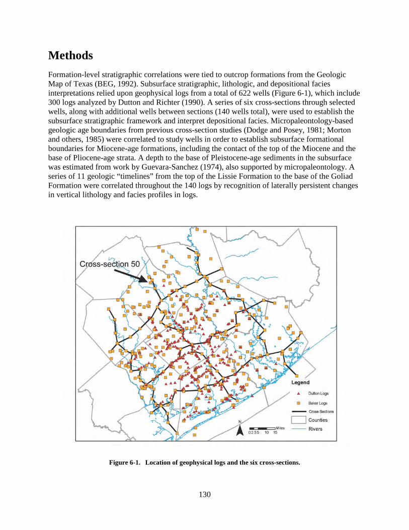
130

Methods Formation-level stratigraphic correlations were tied to outcrop formations from the Geologic Map of Texas (BEG, 1992). Subsurface stratigraphic, lithologic, and depositional facies interpretations relied upon geophysical logs from a total of 622 wells (Figure 6-1), which include 300 logs analyzed by Dutton and Richter (1990). A series of six cross-sections through selected wells, along with additional wells between sections (140 wells total), were used to establish the subsurface stratigraphic framework and interpret depositional facies. Micropaleontology-based geologic age boundaries from previous cross-section studies (Dodge and Posey, 1981; Morton and others, 1985) were correlated to study wells in order to establish subsurface formational boundaries for Miocene-age formations, including the contact of the top of the Miocene and the base of Pliocene-age strata. A depth to the base of Pleistocene-age sediments in the subsurface was estimated from work by Guevara-Sanchez (1974), also supported by micropaleontology. A series of 11 geologic “timelines” from the top of the Lissie Formation to the base of the Goliad Formation were correlated throughout the 140 logs by recognition of laterally persistent changes in vertical lithology and facies profiles in logs.

Figure 6-1. Location of geophysical logs and the six cross-sections.

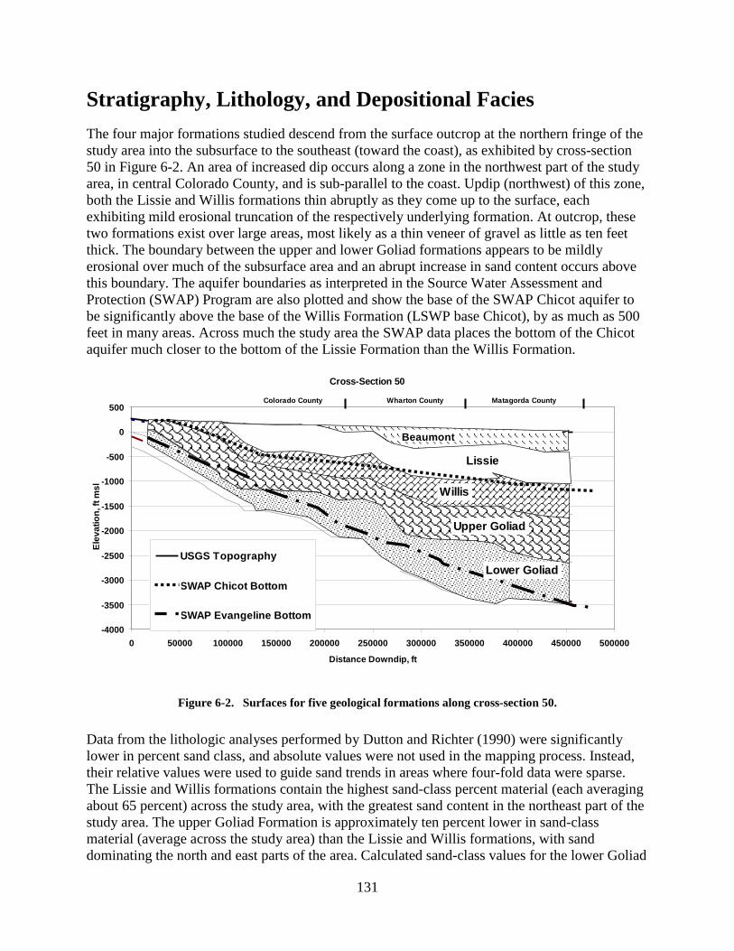
131

Stratigraphy, Lithology, and Depositional Facies The four major formations studied descend from the surface outcrop at the northern fringe of the study area into the subsurface to the southeast (toward the coast), as exhibited by cross-section 50 in Figure 6-2. An area of increased dip occurs along a zone in the northwest part of the study area, in central Colorado County, and is sub-parallel to the coast. Updip (northwest) of this zone, both the Lissie and Willis formations thin abruptly as they come up to the surface, each exhibiting mild erosional truncation of the respectively underlying formation. At outcrop, these two formations exist over large areas, most likely as a thin veneer of gravel as little as ten feet thick. The boundary between the upper and lower Goliad formations appears to be mildly erosional over much of the subsurface area and an abrupt increase in sand content occurs above this boundary. The aquifer boundaries as interpreted in the Source Water Assessment and Protection (SWAP) Program are also plotted and show the base of the SWAP Chicot aquifer to be significantly above the base of the Willis Formation (LSWP base Chicot), by as much as 500 feet in many areas. Across much the study area the SWAP data places the bottom of the Chicot aquifer much closer to the bottom of the Lissie Formation than the Willis Formation.

Cross-Section 50

-4000

-3500

-3000

-2500

-2000

-1500

-1000

-500

0

500

0 50000 100000 150000 200000 250000 300000 350000 400000 450000 500000

Distance Downdip, ft

Elev

atio

n, ft

msl

USGS Topography

SWAP Chicot Bottom

SWAP Evangeline Bottom

Colorado County Wharton County Matagorda County

Beaumont

Lissie

Willis

Upper Goliad

Lower Goliad

Figure 6-2. Surfaces for five geological formations along cross-section 50.

Data from the lithologic analyses performed by Dutton and Richter (1990) were significantly lower in percent sand class, and absolute values were not used in the mapping process. Instead, their relative values were used to guide sand trends in areas where four-fold data were sparse. The Lissie and Willis formations contain the highest sand-class percent material (each averaging about 65 percent) across the study area, with the greatest sand content in the northeast part of the study area. The upper Goliad Formation is approximately ten percent lower in sand-class material (average across the study area) than the Lissie and Willis formations, with sand dominating the north and east parts of the area. Calculated sand-class values for the lower Goliad

132

Formation are about seven percent lower than those for the upper Goliad Formation, with a series of distinctly sandier areas trending northwest to southeast across the study area. The differences in the sand-class distributions produced for the Willis and upper Goliad formations are shown in Figure 6-3. The sand-class data provide potentially pertinent information regarding the discrepancy between the base of the Chicot aquifer in this study and that in the SWAP dataset. Sand-class values were tabulated for the Chicot and Evangeline aquifers using the aquifer boundaries from the SWAP dataset and those from this study (Table 6-1). As noted by Baker (1979), Jorgensen (1975), and Carr and others (1985), the Chicot aquifer is conceptually distinguished from the Evangeline aquifer by its distinctly greater hydraulic conductivity, which equates to greater sand percent. Table 6-1 was created to help quantify the difference in the sand-class distributions between the Chicot and Evangeline aquifers in order to provide a framework for deciding whether or not our representation of the boundary of the base of the Chicot aquifer is reasonable. In Table 6-1, the “LSWP-SWAP” interval is the aquifer volume sandwiched between the two approximations of the base of the Chicot aquifer across the study area. Logs used by Dutton and Richter (1990) the “LSWP-SWAP” interval have nearly the same sand-class distribution as the Chicot aquifer for both sets of boundaries. For the LSWP logs, the “LSWP-SWAP” interval’s sand-class distribution is intermediate to the distributions for the two aquifers but is significantly closer to the distributions for the Chicot aquifer than for the Evangeline aquifer. Hence, it would appear that, if the two aquifers are differentiated based on permeability, our base for Chicot aquifer is justified and defensible.

Geophysical log profiles for each of the formations were interpreted as reflecting a regional depositional transition from fluvial channel and intervening floodplain facies updip (northwestward) to a mixture of bayfill, coastal, incised valley, and shelf facies downdip (toward the current shoreline). Fluvial channel facies vary from broad, sand-dominated regions, such as in the northwest area of the Lissie Formation (Figure 6-4a), to a series of narrow northwest-southeast trending areas, such as in the northwest part of the Willis Formation (Figure 6-3a).

Figure 6-3. Sand-class distribution maps for the Willis and upper Goliad formations.

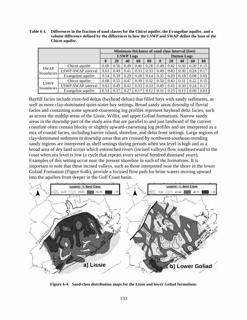
133

Table 6-1. Differences in the fraction of sand classes for the Chicot aquifer, the Evangeline aquifer, and a volume difference defined by the differences in how the LSWP and SWAP define the base of the Chicot aquifer.

Minimum thickness of sand class interval (feet) LSWP Logs Dutton Logs

0 20 40 60 80 0 20 40 60 80

SWAP boundaries

Chicot aquifer 0.69 0.56 0.49 0.40 0.28 0.49 0.42 0.30 0.20 0.15 LSWP-SWAP interval 0.63 0.49 0.41 0.33 0.33 0.49 0.43 0.30 0.24 0.17

Evangeline aquifer 0.54 0.39 0.29 0.20 0.14 0.35 0.29 0.18 0.08 0.05

LSWP boundaries

Chicot aquifer 0.68 0.55 0.47 0.39 0.32 0.50 0.43 0.31 0.22 0.15 LSWP-SWAP interval 0.63 0.49 0.41 0.33 0.33 0.49 0.43 0.30 0.24 0.17

Evangeline aquifer 0.52 0.37 0.27 0.17 0.12 0.31 0.25 0.13 0.06 0.03

Bayfill facies include river-fed deltas (bayhead deltas) that filled bays with sandy sediments, as well as more clay-dominated quiet-water bay settings. Broad sandy areas downdip of fluvial facies and containing some upward-coarsening log profiles represent bayhead delta facies, such as across the middip areas of the Lissie, Willis, and upper Goliad formations. Narrow sandy areas in the downdip part of the study area that are parallel to and just landward of the current coastline often contain blocky or slightly upward-coarsening log profiles and are interpreted as a mix of coastal facies, including barrier island, shoreline, and delta front settings. Large regions of clay-dominated sediment in downdip areas that are crossed by northwest-southeast-trending sandy regions are interpreted as shelf settings during periods when sea level is high and as a broad area of dry land across which entrenched rivers (incised valleys) flow southeastward to the coast when sea level is low (a cycle that repeats every several hundred thousand years). Examples of this setting occur near the present shoreline in each of the formations. It is important to note that these incised valleys, such as those interpreted near the shore in the lower Goliad Formation (Figure 6-4b), provide a focused flow path for brine waters moving upward into the aquifers from deeper in the Gulf Coast basin.

a) Lissie b) Lower Goliada) Lissiea) Lissie b) Lower Goliadb) Lower Goliad

Figure 6-4. Sand-class distribution maps for the Lissie and lower Goliad formations.

134

Aquifer Summary The Chicot and Evangeline aquifers in the LSWP study area have been subdivided into the upper Chicot (Lissie Formation), lower Chicot (Willis Formation), upper Evangeline (upper Goliad Formation), and lower Evangeline (lower Goliad Formation), using formation boundaries and geologic timelines established by outcrop geology and micropaleontologic evidence from the subsurface. The upper and lower Chicot aquifers are distinctly sandier than the upper Evangeline aquifer, which in turn is sandier than the lower Evangeline aquifer. Sand content of the Chicot and upper Evangeline aquifers is greatest in the updip half of the study area, whereas no specific area of sandiness is seen in the lower Evangeline aquifer. The sandiest areas in both aquifers may be narrow, on the order of ten miles wide, and strongly northeast-southwest trending. This trend reflects a series of sedimentary depositional settings from fluvial in the updip (northwest) area to bayfill in the middip, and a mix of coastal, incised valley, and shelf in the downdip (southeast) area.

The Chicot-Evangeline aquifer boundary interpreted here is above that established in the SWAP dataset over much of the study area by amounts up to 500 feet. Although analysis of lithologic data tends to support the LSWP boundary, more study may be needed to understand this discrepancy and to evaluate it in a broader geographic context.

Data Sources Related to Hydraulic Conductivity Values To estimate the spatial variability in the hydraulic conductivity field across the study area, we used transmissivity values, specific capacity values, sand distribution maps, and depositional facies maps. Transmissivity values were collected from two sources. One source consisted of tabulated transmissivity values from U.S. Geological Survey and Texas Water Development Board reports. The other source consisted of transmissivity values calculated from pumping test data obtained from the Texas Commission on Environmental Quality’s Division of Water Supply. The specific capacity values were calculated from information collected from water driller logs at the Texas Ccommission on Environmental Quality. The sand distribution and facies maps were developed from analyses of geophysical logs.

Screen Length Effect on Hydraulic Conductivity Estimates

The method of Meyers (1969) was used to calculate hydraulic conductivity from approximately 400 pumping tests. Figure 6-5 shows how the mean calculated hydraulic conductivity values change as a function of screen length. The figure shows a nearly exponential decrease of hydraulic conductivity with increases in screen length. Relative changes in normalized specific capacity values (specific capacity divided by screen length) can be used to approximate relative changes in hydraulic conductivity values. Figure 6-6 shows the average normalized specific capacity as a function of well screen length. In general, the trends are consistent with the trends obtained with the hydraulic conductivity data set shown in Figure 6-5.

We attribute the observed trends in Figures 6-5 and 6-6 to three causes. The first cause is that the process involved with locating a well screen is not a random process, but rather a very biased and

135

Figure 6-5. Relationship between hydraulic Figure 6-6. Relationship between normalized conductivity and well screen length. specific capacity and well screen length.

systematic process aimed at placing the well screen into one of the aquifer’s more permeable intervals. Typically, drillers install well screens across the first reliable producing zone that will meet the needs of a client. As the well screen length becomes large with respect to the average thickness of the aquifer, the opportunity for the well screen to intersect moderate to low permeability deposits increases. Consequently, hydraulic conductivity values calculated from pumping wells with small well screens will likely be higher than the average hydraulic conductivity of the aquifer. In addition, the calculated hydraulic conductivity is likely to be more representative of the aquifer as a whole as the length of the well screen approaches the thickness of the aquifer. The second cause for the observed trends in Figures 6-5 and 6-6 is that smaller well screens tend to promote non-lateral flow toward a well, which violates the assumption of the Meyers (1969) method and thereby leads to overestimation of the hydraulic conductivity. The third cause is that a decreasing trend in hydraulic conductivity with depth may be contributing to the asymptotic behavior at large screen lengths. One of the factors that could lead to a decrease trend in hydraulic conductivity with depth is increased compaction of sediments with depth.

Hydraulic Conductivity Values

Hydraulic conductivity values used to constrain a model’s calibration should be representative of a scale that is consistent with the volume and size of the numerical model’s grid. Most of the model grids in the LSWP groundwater model will be greater than 300 feet thick. In order to account for the well screen length bias shown in Figures 6-5 and 6-6, we used a minimum cut-off well screen length of 150 feet to develop a set of values for the model calibration (Table 6-2). The results in the table demonstrate that the selection criteria have a significant impact on both the magnitudes of the averages as well as the relative differences in the averages among the different counties. One of the effects of the filtering is to change the location of the highest averages from Brazoria and Galveston counties to Wharton and Fort Bend counties.

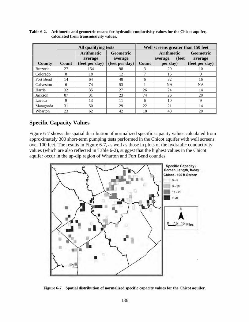
136

Table 6-2. Arithmetic and geometric means for hydraulic conductivity values for the Chicot aquifer, calculated from transmissivity values.

County

All qualifying tests Well screens greater than 150 feet

Count

Arithmetic average

(feet per day)

Geometric average

(feet per day) Count

Arithmetic average (feet

per day)

Geometric average

(feet per day) Brazoria 27 154 98 3 20 10 Colorado 8 18 12 7 15 9 Fort Bend 14 64 48 6 32 16 Galveston 6 74 53 1 NA NA Harris 32 35 27 26 24 14 Jackson 87 31 23 74 26 20 Lavaca 9 13 11 6 10 9 Matagorda 31 50 29 22 21 14 Wharton 23 62 42 18 48 20

Specific Capacity Values

Figure 6-7 shows the spatial distribution of normalized specific capacity values calculated from approximately 300 short-term pumping tests performed in the Chicot aquifer with well screens over 100 feet. The results in Figure 6-7, as well as those in plots of the hydraulic conductivity values (which are also reflected in Table 6-2), suggest that the highest values in the Chicot aquifer occur in the up-dip region of Wharton and Fort Bend counties.

Figure 6-7. Spatial distribution of normalized specific capacity values for the Chicot aquifer.

137

Correlation between Lithology and Hydraulic Conductivity

To investigate correlations between lithology and hydraulic conductivity in the Chicot aquifer, we assembled data for 48 wells with reliable pumping test data and lithologic information. Using data from these 48 wells, we developed an equation for predicting average hydraulic conductivity based primarily on the percent sands in the deposit that the well screen intersects. Minor adjustments existed in the equation to account for the thicknesses of the clay and sand beds. Based on the lithologic logs of these wells, the average sand content in the Chicot aquifer is 53 percent and an approximate average hydraulic conductivity for sand is approximately 32 feet per day. As designed, the equation matches the average hydraulic conductivity of the 48 pumping tests, which is 19 feet per day. The regression analysis indicates that for most of the Chicot aquifer, the percent sand coverage is a reasonable indicator of average hydraulic conductivity.

The analysis of the geophysical logs for lithology involved categorizing the interpreted lithology into sand and clay classes. Our sand class, for instance, indicates that a deposit is composed of 50 to 100 percent sands. Figure 6-8 shows the distribution of the thicknesses associated with the sand class coverage by county. These results, in combination with results from our regression analysis, indicate the highest hydraulic conductivity values should occur within Wharton and Fort Bend counties.

Analysis of the geophysical logs also involved developing chronostratigraphy surfaces and maps of depositional facies. Within the Chicot aquifer, there are significant differences among the counties regarding the depositional facies associated with the Chicot aquifer. The two counties having a distribution of facies most conducive to producing permeable deposits are Wharton and Fort Bend counties.

0%

10%

20%

30%

40%

50%

60%

70%

80%

Colorado Fort Bend Wharton Jackson Matagorda Brazoria

% C

over

age

20-4040-6060-80>80

Bed Thickness

(ft)

Figure 6-8. Distribution of the bed thicknesses of sand class beds in the Chicot aquifer.

138

Hydraulic Conductivity Summary Multiple data sources and analysis approaches were investigated for developing estimates of spatial variability in the hydraulic conductivity field of the Chicot aquifer in the study area for the LSWP. All of the methods produced valuable information, most of which is consistent and useful for guiding the development of the groundwater flow model. All methods indicate that the highest average hydraulic conductivity values in the Chicot aquifer exist in Wharton and Fort Bend counties. Young and Kelley (2005) provide additional details regarding the results.

References Baker, E. T., Jr., 1979, Stratigraphic and hydrogeologic framework of part of the Coastal Plain of

Texas: Texas Department of Water Resources Report 236, 43 p.

BEG, 1992, Geologic Map of Texas: compiled by V. E. Barnes, the University of Texas at Austin, Bureau of Economic Geology, State map No. 3, Scale 1:500,000.

Carr, J. E., Meyer, W. R., Sandeen, W. M., and McLane, I. R., 1985, Digital models for simulation of ground-water hydrology of the Chicot and Evangeline aquifers along the Gulf Coast of Texas: Texas Department of Water Resources Report 289, 101 p.

Dodge, M. M., and Posey, J. S., 1981, Structural cross sections, Tertiary formations, Texas Gulf Coast: The University of Texas at Austin, Bureau of Economic Geology Cross Section Series No. 2, 6 p.

Dutton, A. R., and Richter, B. C., 1990, Regional geohydrology of the Gulf Coast aquifer in Matagorda and Wharton counties—Development of a numerical model to estimate the impact of water-management strategies: Contract report prepared for Lower Colorado River Authority, Austin, Texas, under Contract IAC (88-89)0910, 116 p.

Guevara-Sanchez, E. H., 1974, Pleistocene facies in the subsurface of the Southeast Texas Coastal Plain: Ph.D. dissertation, The University of Texas at Austin, 133 p.

Jorgensen, D. G., 1975, Analog-model studies of ground-water hydrology in the Houston District, Texas: Texas Water Development Board Report 190, 84 p.

Morton, R. A., Jirik, L. A., and Foote, R. Q., 1985, Structural cross sections, Miocene series, Texas continental shelf: The University of Texas at Austin, Bureau of Economic Geology Cross Section Series No. 5, 8 p.

Meyers, B. N., 1969, Compilation of results of aquifer tests in Texas: U.S. Geological Survey Report 98, 147 p.

Young, S. C., and Kelly, V., editors, 2005, Draft—A site conceptual model to support the development of a detailed groundwater model for Colorado, Wharton, and Matagorda counties: prepared for the Lower Colorado River Authority, Austin, Texas.

139

Chapter 7

100 Years of Groundwater Use and Subsidence in the Upper Texas Gulf Coast

Thomas A. Michel1

Introduction Imagine yourself more than a hundred years ago, living in southeastern Texas. You would have faced many challenges, among others: 100 degree temperatures and 80 percent humidity in the summers, ruthless mosquitoes, roaming alligators, and a whole host of other challenges of the early 20th century that we do not worry about today. One challenge that residents of Galveston, Houston, and the surrounding area did not have to face was water. Water was already distributed throughout the area, underground, in what is today referred to as the Gulf Coast Aquifer System. It was only necessary to drill a shallow well and clean groundwater would flow from the well, even without a pump to withdraw it. Water was abundant.

Today, in the early 21st century, we have air conditioners that counteract the heat and humidity of the summer months, government trucks that spray pesticides to greatly reduce the mosquito population, and for whatever reasons the alligators don’t seem to roam the streets of downtown Houston as they once did. Oh, how the times have changed. As the population grew throughout the last century and industries blossomed, the demand for water increased greatly. Unlike 100 years ago, one of our greatest challenges today is our water supply. You can’t just drill a shallow well today in your backyard anymore and expect clean, fresh water to come bubbling up.

In today’s greater Houston area, groundwater still is utilized by many people, but surface water is the predominant supply. Years of increasing demand for groundwater caused irreversible harm to the area and measures were taken to combat the problems caused by the over-reliance of groundwater. So far, the efforts have been a great success story for the area and residents of yesterday should be appreciated for their foresight in developing surface water supplies such as Lakes Conroe, Houston, and Livingston. Residents of today’s greater Houston area should be thanked for their continued efforts to provide for a reliable and sustainable water supply. Those residents yet to arrive to the area need to be reminded of the challenges faced and overcome, but also reminded that we will always need to protect our environment from our insatiable thirst for water.

1 Harris-Galveston Subsidence District

140

The Rise and Fall of Groundwater Pumpage At the beginning of the 20th Century, the rather small City of Houston was primarily an agricultural area with a population of only 45,000 people. The area gained national recognition due largely to the devastation of the Great Storm of 1900 and the many lives that were lost. The City of Galveston lost about one-sixth of its population in the storm, but the misfortunes of Galveston led to the beginnings of a boom in population that Houston has sustained even to today.

Water from underground in the Gulf Coast Aquifer System was utilized as the predominant water supply. The system is made up of layers of clays and sands with no stable rock within the primary pumping strata. Groundwater from the Chicot and Evangeline aquifers, within the aquifer system, provided the necessary water for developing industries and the population necessary to support those industries. The Chicot aquifer is the shallower aquifer within the Gulf Coast Aquifer System, with the Evangeline aquifer beneath the Chicot (Figure 7-1). Generally, the Chicot aquifer has served the water needs of the southeastern portion of Harris County and Galveston County while the deeper Evangeline served the needs of central, north, and west Harris County.

Municipal and industrial water needs began to rise with the oil boom in the early 1900s and the development of the Houston Ship Channel. The Port of Houston Authority was created in 1927 by the Texas Legislature, thus beginning the real boom in industry around the Houston Ship Channel. Post-World War II, Houston’s economy had almost entirely switched from agriculture to the oil and gas industries and other emerging industries such as plastics. Historically, all of these industries and the surrounding municipal use were supplied with water from the Chicot and Evangeline aquifers.

Figure 7-1. Illustrated cross-section of the Gulf Coast Aquifer System.

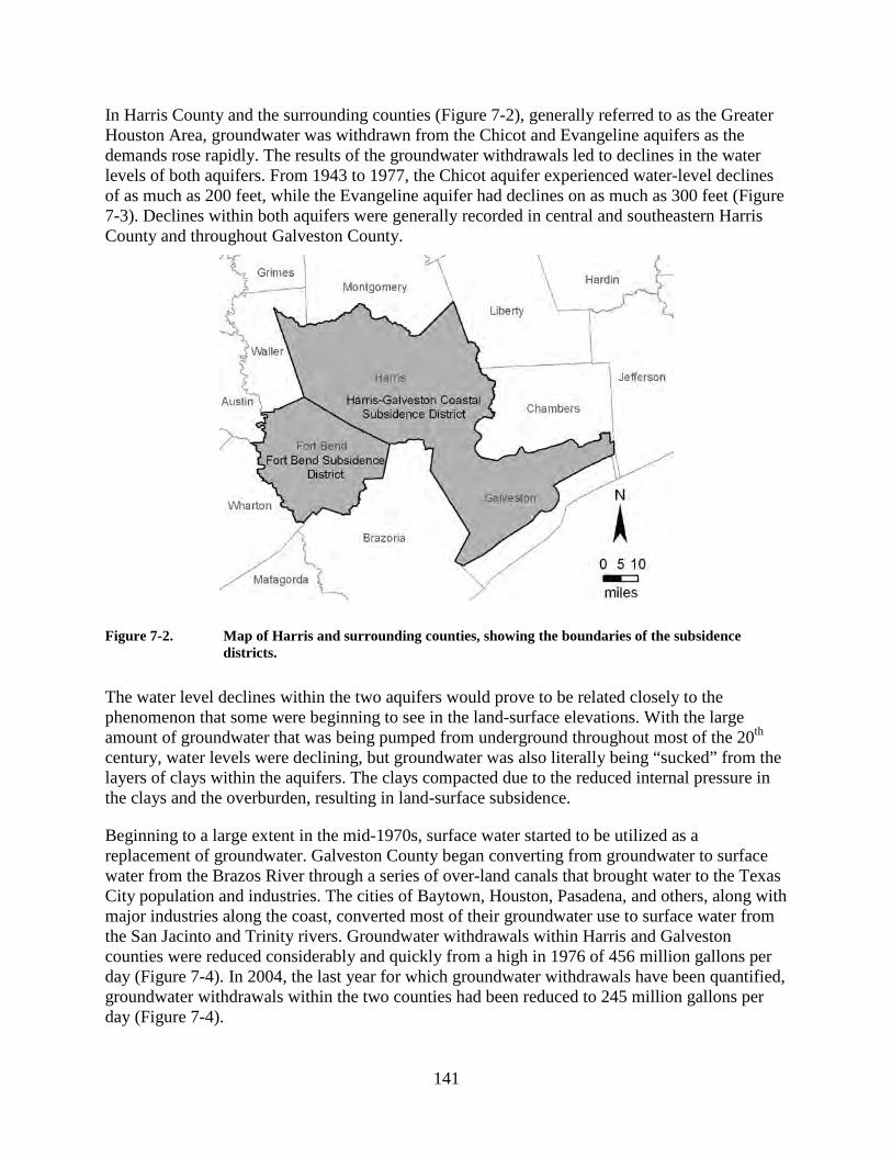
141

In Harris County and the surrounding counties (Figure 7-2), generally referred to as the Greater Houston Area, groundwater was withdrawn from the Chicot and Evangeline aquifers as the demands rose rapidly. The results of the groundwater withdrawals led to declines in the water levels of both aquifers. From 1943 to 1977, the Chicot aquifer experienced water-level declines of as much as 200 feet, while the Evangeline aquifer had declines on as much as 300 feet (Figure 7-3). Declines within both aquifers were generally recorded in central and southeastern Harris County and throughout Galveston County.

Figure 7-2. Map of Harris and surrounding counties, showing the boundaries of the subsidence districts.

The water level declines within the two aquifers would prove to be related closely to the phenomenon that some were beginning to see in the land-surface elevations. With the large amount of groundwater that was being pumped from underground throughout most of the 20th century, water levels were declining, but groundwater was also literally being “sucked” from the layers of clays within the aquifers. The clays compacted due to the reduced internal pressure in the clays and the overburden, resulting in land-surface subsidence.

Beginning to a large extent in the mid-1970s, surface water started to be utilized as a replacement of groundwater. Galveston County began converting from groundwater to surface water from the Brazos River through a series of over-land canals that brought water to the Texas City population and industries. The cities of Baytown, Houston, Pasadena, and others, along with major industries along the coast, converted most of their groundwater use to surface water from the San Jacinto and Trinity rivers. Groundwater withdrawals within Harris and Galveston counties were reduced considerably and quickly from a high in 1976 of 456 million gallons per day (Figure 7-4). In 2004, the last year for which groundwater withdrawals have been quantified, groundwater withdrawals within the two counties had been reduced to 245 million gallons per day (Figure 7-4).

142

Figure 7-3. Evangeline aquifer, water-level declines 1943–1977 (Kasmarek, 2005).

As the population in the greater Houston area exploded and overtook historically agricultural lands, agricultural use diminished to only five percent of the total groundwater usage (light grey bars—Figure 7-4). Industrial groundwater usage (dark grey bars—Figure 7-4) decreased rapidly with the introduction of surface water in the mid-1970s and makes up only six percent of the 2004 total groundwater produced. While municipal groundwater use in Galveston County and the central and southeastern portions of Harris County decreased dramatically from the mid-1970s, the northern and western portions of Harris County continued to grow on groundwater. In 2004 municipal groundwater use (black bars—Figure 7-4) made up nearly 90 percent of the total groundwater production in Harris and Galveston counties, with about 220 million gallons per day being pumped from the unconverted northern and western Harris County.

Hopefully, groundwater usage in Harris and Galveston counties has seen its high point. With the groundwater regulations that face the area, more conversions from groundwater to surface water are just around the corner. By the year 2010, north and west Harris County will join the others within the greater area with a 30 percent reduction in groundwater use. By the year 2030, total groundwater usage within Harris and Galveston County should be far less than 20 percent of total water demand.

Tale of the Subsidence District Around 1920, in the Goose Creek Oil Field in Baytown, Texas, on the Gaillard Peninsula, oil and gas was beginning to be rapidly withdrawn from relatively shallow wells. In 1926, Wallace Pratt

143

Figure 7-4. Groundwater pumpage 1976 to 2004, Harris and Galveston counties.

and Douglas Johnson published the first known documentation of subsidence (Pratt and Johnson, 1926). Pratt and Johnson documented roughly three feet of subsidence in a very localized area over an eight year period from 1917 to 1925. The oil and gas was being withdrawn from a depth about twice that from which water would eventually be pumped.

Pratt and Johnson were the first authors of a subject that would unfortunately lie dormant in the area for roughly 50 years. Again, the Baytown area took center-stage. The Brownwood Subdivision is a very nice subdivision on a peninsula along the San Jacinto River within about five miles of the Goose Creek Oil Field. In the late 1950s and early 1960s, residents of Brownwood had a sinking feeling. They noticed that the water was rising. In reality the water wasn’t rising—the land was sinking. It would take Hurricane Carla in 1961 to bring serious attention to the problem of subsidence in Baytown and other areas around Houston. Texas City, which was just a little higher than sea level in some areas in the 1960s, began noticing that elevations were changing. Industries along the Houston Ship Channel were finding that the ships they were servicing in the Ship Channel were increasingly higher than the docks and loading facilities.

Pratt and Johnson had touched on a cause and effect. When fluids were withdrawn from the compactable subsurface, compaction would result and the land surface would subside. The trouble with their work in the late 1920s was that it was focused on oil and gas production and not water. Excessive groundwater withdrawals would be found to be the culprit of the vast majority subsidence throughout the greater Houston area. By the late 1970s, subsidence had surpassed nine feet along the Houston Ship Channel and as much as five feet in the Texas City area, with a large part of Harris County experiencing at least one foot of subsidence (Figure 7-5).

In 1975, the 64th Texas Legislature created the Harris-Galveston Coastal Subsidence District (the District). In 2005, the Legislature modified the District’s enabling act, removing the word

144

“coastal” from the name and placing the District within Chapter 8801 of the Special Districts Code. The purpose of the District has always remained as the need to regulate groundwater withdrawals as they relate to land-surface subsidence in Harris and Galveston counties. In 1990,

Figure 7-5. Subsidence, 1906 to 1978.

the Legislature created the Fort Bend Subsidence District, and the two Districts cooperate on an annual basis to halt subsidence within Fort Bend, Galveston, and Harris counties. The District immediately began a permitting effort to require permits for non-private household water wells and called for the installation of meters on virtually all permitted wells.

The District then set out on the task of understanding all of the technical factors associated with groundwater withdrawal. They began studies to determine the relationships between withdrawals, water-level declines, compaction of the subsurface clay layers, and the land-surface elevations. The District started a wide area water-level monitoring network with the U.S. Geological Survey in 1977 for the Chicot and Evangeline aquifers. The District also established a strong relationship with the National Geodetic Survey to conduct accurate first-order benchmark re-levelings throughout the area.

The District’s first major regulatory effort was the adoption of the 1976 Regulatory Plan. Due to the infancy of the District, the 1976 Plan was not a “mandate” but rather a suggestion or plea to the major permittees along the coast. The 1976 Plan mapped out an area that a storm surge of 15 feet would inundate and labeled it the Area of Concentrated Emphasis (ACE). Within the ACE, the District called upon permittees to voluntarily do whatever they could to reduce groundwater withdrawals. Cities and industries had already begun to realize the effects of their groundwater withdrawals and started to convert to alternative water supplies.

In 1985, after a number of years of collecting data and studying the relationship between groundwater and subsidence, the District adopted the first mandated groundwater reductions. The 1985 Regulatory Plan borrowed upon the ACE and mapped out what is still referred to as Regulatory Areas 1 and 2. There were eight regulatory areas in total, all with groundwater

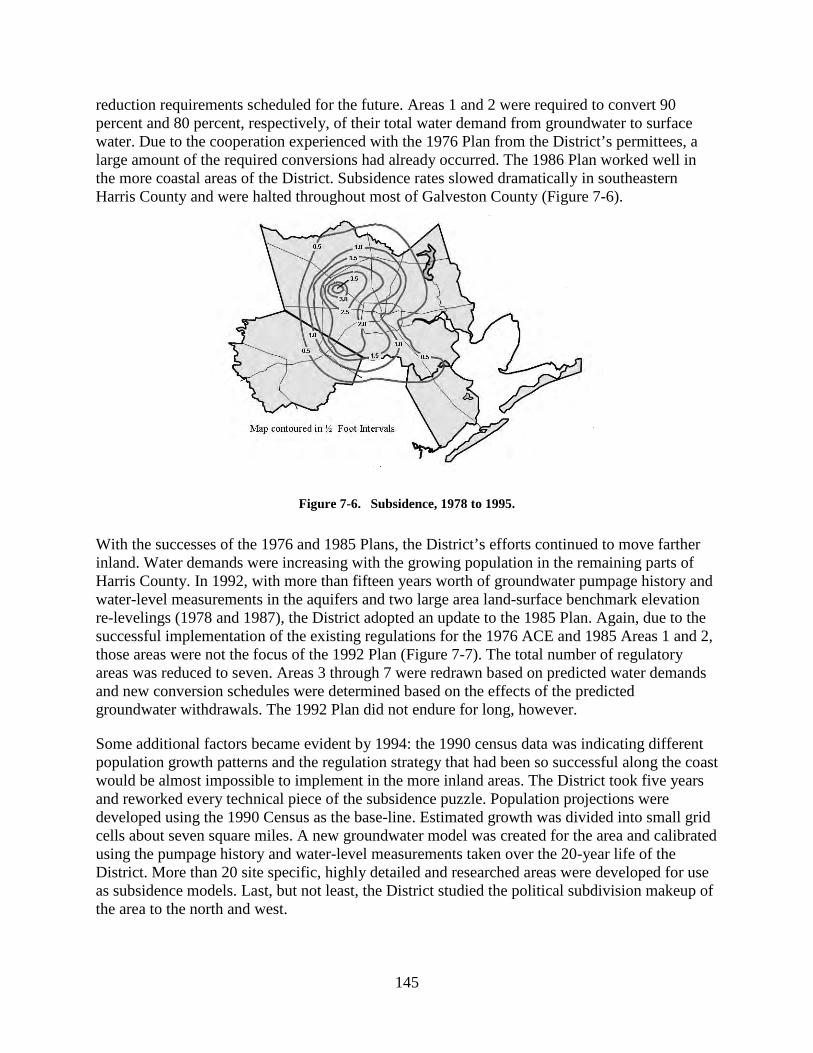
145

reduction requirements scheduled for the future. Areas 1 and 2 were required to convert 90 percent and 80 percent, respectively, of their total water demand from groundwater to surface water. Due to the cooperation experienced with the 1976 Plan from the District’s permittees, a large amount of the required conversions had already occurred. The 1986 Plan worked well in the more coastal areas of the District. Subsidence rates slowed dramatically in southeastern Harris County and were halted throughout most of Galveston County (Figure 7-6).

Figure 7-6. Subsidence, 1978 to 1995.

With the successes of the 1976 and 1985 Plans, the District’s efforts continued to move farther inland. Water demands were increasing with the growing population in the remaining parts of Harris County. In 1992, with more than fifteen years worth of groundwater pumpage history and water-level measurements in the aquifers and two large area land-surface benchmark elevation re-levelings (1978 and 1987), the District adopted an update to the 1985 Plan. Again, due to the successful implementation of the existing regulations for the 1976 ACE and 1985 Areas 1 and 2, those areas were not the focus of the 1992 Plan (Figure 7-7). The total number of regulatory areas was reduced to seven. Areas 3 through 7 were redrawn based on predicted water demands and new conversion schedules were determined based on the effects of the predicted groundwater withdrawals. The 1992 Plan did not endure for long, however.

Some additional factors became evident by 1994: the 1990 census data was indicating different population growth patterns and the regulation strategy that had been so successful along the coast would be almost impossible to implement in the more inland areas. The District took five years and reworked every technical piece of the subsidence puzzle. Population projections were developed using the 1990 Census as the base-line. Estimated growth was divided into small grid cells about seven square miles. A new groundwater model was created for the area and calibrated using the pumpage history and water-level measurements taken over the 20-year life of the District. More than 20 site specific, highly detailed and researched areas were developed for use as subsidence models. Last, but not least, the District studied the political subdivision makeup of the area to the north and west.

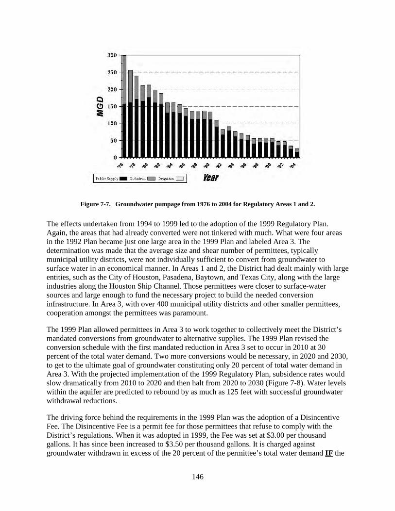
146

Figure 7-7. Groundwater pumpage from 1976 to 2004 for Regulatory Areas 1 and 2.

The effects undertaken from 1994 to 1999 led to the adoption of the 1999 Regulatory Plan. Again, the areas that had already converted were not tinkered with much. What were four areas in the 1992 Plan became just one large area in the 1999 Plan and labeled Area 3. The determination was made that the average size and shear number of permittees, typically municipal utility districts, were not individually sufficient to convert from groundwater to surface water in an economical manner. In Areas 1 and 2, the District had dealt mainly with large entities, such as the City of Houston, Pasadena, Baytown, and Texas City, along with the large industries along the Houston Ship Channel. Those permittees were closer to surface-water sources and large enough to fund the necessary project to build the needed conversion infrastructure. In Area 3, with over 400 municipal utility districts and other smaller permittees, cooperation amongst the permittees was paramount.

The 1999 Plan allowed permittees in Area 3 to work together to collectively meet the District’s mandated conversions from groundwater to alternative supplies. The 1999 Plan revised the conversion schedule with the first mandated reduction in Area 3 set to occur in 2010 at 30 percent of the total water demand. Two more conversions would be necessary, in 2020 and 2030, to get to the ultimate goal of groundwater constituting only 20 percent of total water demand in Area 3. With the projected implementation of the 1999 Regulatory Plan, subsidence rates would slow dramatically from 2010 to 2020 and then halt from 2020 to 2030 (Figure 7-8). Water levels within the aquifer are predicted to rebound by as much as 125 feet with successful groundwater withdrawal reductions.

The driving force behind the requirements in the 1999 Plan was the adoption of a Disincentive Fee. The Disincentive Fee is a permit fee for those permittees that refuse to comply with the District’s regulations. When it was adopted in 1999, the Fee was set at $3.00 per thousand gallons. It has since been increased to $3.50 per thousand gallons. It is charged against groundwater withdrawn in excess of the 20 percent of the permittee’s total water demand IF the

147

Figure 7-8. Predicted subsidence assuming implementation of the 1999 Regulatory Plan.

permittee has not complied with the District’s regulations. The Disincentive Fee went into effect for Areas 1 and 2 in 2001 and for Area 3 in 2003. To avoid the Disincentive Fee, a permittee could remain at or below the allowable limit of groundwater: 10 percent for Area 1, 20 percent for Area 2, and 20 percent for Area 3. In Area 3, permittees could also avoid the Disincentive Fee between 2003 and 2010 by developing and implementing a Groundwater Reduction Plan that outlined how the permittee would meet the 2010, 2002, and 2030 reduction requirements.

The District’s 1999 Regulatory Plan has been very successful. Groundwater withdrawals have already begun to decline in Area 3, more than five years ahead of schedule. Permittees have worked together to form collective Groundwater Reduction Plans, most notably the North Harris County Regional Water Authority, the West Harris County Regional Water Authority, the City of Houston and the permittees that have joined with Houston, and other smaller individual and combinations of permittees. To the District’s delight, very few Disincentive Fees have had to be issued. Since 2001, only about $500,000 in Disincentive Fees have had to be billed and collected in total out of a potential for $60 million annually.

Conclusion The Harris-Galveston Subsidence District is celebrating its 30th Anniversary in 2005. In thirty years, the District has permitted over 10,000 water wells within its two counties, aided in the creation and operation of the Fort Bend Subsidence District, assisted in the monitoring of more than 500 water wells annually, conducted three major first-order benchmark re-levelings from stable inland elevations, led in the development of new technologies such as GPS to measure subsidence, been involved with six generations of groundwater models, and worked and reworked four major regulatory plans. The District has been responsible for the development of the regulations which required the conversion of millions of gallons daily from groundwater sources to surface water sources. The historical cost of the District’s regulations in today’s dollars would surely be in the billions. The cost of the District’s regulations to the residents of

148

today and tomorrow will be even greater. The District has never taken its mission lightly and certainly understands the magnitude of the impacts of its regulations. The real successes are the motivating factors.

Due to the successes of the past, some would believe subsidence is something to read about in history books. One only needs to look at places such as Baytown, Texas City, and the Houston Ship Channel to see the effects of subsidence. While subsidence has been halted in those areas, new generations must be reminded of the problems of over-relying on groundwater as a source of water. The residents of the greater Houston area have accepted the challenge of combating subsidence and are moving forward. Nothing can be done about the subsidence that has already occurred. The mission of the Subsidence District is to prevent future subsidence. The risks of failing are too great to sit back and admire previous accomplishments. More data is being collected today than ever before. A greater understanding of the relationships between groundwater pumpage and subsidence has never existed before. The tools of today, necessary to predict future water-level changes and subsidence, have never been more accurate. The District’s policy makers of tomorrow will have the best data and tools available to them to make the difficult decisions about groundwater management in the greater Houston area. They will have to always be looking to the past to understand how the future will unfold, but looking to the future to see how they can understand the past better.

Cited References and References of Interest Pratt, W. E., and Johnson, D. W., 1926, Local subsidence of the Goose Creek oil field: Journal of

Geology, v. 34, no. 7, p. 577–590.

Kasmarek, M. C., 2005, U.S. Geological Survey, Open File Report 2005-1128.

Harris-Galveston Coastal Subsidence District, 2005, Annual Groundwater Report, 2005.

Harris-Galveston Coastal Subsidence District, 2003, District Regulatory Plan—1999, revised.

Harris-Galveston Coastal Subsidence District, 1998, Groundwater Management Plan.

Texas Special Districts Code Ann. Ch. 8801.

Prince, K. R., and Galloway, D. L., editors, 2003, U.S. Geological Survey subsidence interest group conference: Galveston, Texas, November 27–29, 2001.

Kasmarek, M. C., and Robinson, J. L., 2004, Hydrology and simulation of ground-water flow and land-surface subsidence in the northern part of the Gulf Coast Aquifer System, Texas: U.S. Geological Survey Scientific Investigations Report 2004–5102, 111 p.

Gabrysch, R. K., and Coplin, L. S., 1990, Land-surface subsidence resulting from ground-water withdrawals in the Houston-Galveston region, Texas, through 1987: Harris–Galveston Coastal Subsidence District and U.S. Geological Survey.

149

Chapter 8

Dry Periods and Drought Events of the Gulf Coastal Region

Robert G. Bradley, P.G.1

Introduction The purpose of this chapter is to describe the dry periods that have occurred and to identify the major drought events along the Gulf Coast of Texas. The Palmer Drought Severity Index and Standardized Precipitation Index will be used to identify major events. A tabulation of dry periods is included as a reference.

The study area is roughly the area coved by the Gulf Coastal plain of Texas (Figure 8-1). Because of the large study area, it covers parts of five climatic divisions (Figure 8-1) as defined by the National Oceanic and Atmospheric Administration. Climatic divisions are reporting regions within a state that are generally climatically homogeneous and are used to report climatic data such as drought indices (NCDC, 1983).

The climate of the study area varies. Average annual precipitation varies from less than 20 inches along the Rio Grande to more than 60 inches along the Sabine River (NCDC, 2002). The eastern two-thirds of the study area have a subtropical humid climate that has warm summers, while the southern third of the area has a subtropical subhumid climate characterized by hot summers and dry winters (Larkin and Bomar, 1983).

Palmer Drought Severity Index Discussions about agricultural, meteorological, or hydrological drought typically look at parts of the hydrological cycle. One misconception is that a specific drought index is the only technique to characterize a drought event. For example, the Palmer Drought Severity Index (PDSI) and most other indices use a single number representing the general dryness conditions at a measurement location.

The PDSI is the most commonly used drought index in the United States. In Texas, it is the standard “Drought Index” for determining dry or drought conditions. Yet, due to the spatial scale

1 Texas Water Development Board

150

Figure 8-1. Study area showing the National Oceanic and Atmospheric Administration climatic divisions and Historical Climatology Network weather stations used in this chapter (NCDC, 1983; Williams and others, 2005).

at which the PDSI is calculated, the index is not suitable for determining local drought conditions.

The PDSI series ranges roughly from -6.0 to +6.0. The base index of the Palmer Index series is called the “Z” index, which is assumed to represent moisture conditions. Palmer (1965) selected the classification scale of moisture conditions based on study areas in Iowa, Kansas, and Texas. A listing of the PDSI classifications is in Table 8-1.

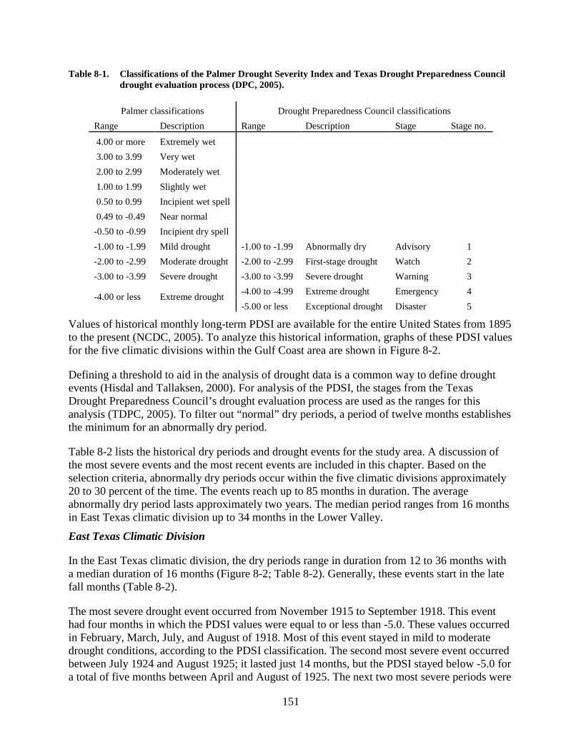
151

Table 8-1. Classifications of the Palmer Drought Severity Index and Texas Drought Preparedness Council drought evaluation process (DPC, 2005).

Palmer classifications Drought Preparedness Council classifications Range Description Range Description Stage Stage no.

4.00 or more Extremely wet 3.00 to 3.99 Very wet 2.00 to 2.99 Moderately wet 1.00 to 1.99 Slightly wet 0.50 to 0.99 Incipient wet spell 0.49 to -0.49 Near normal -0.50 to -0.99 Incipient dry spell -1.00 to -1.99 Mild drought -1.00 to -1.99 Abnormally dry Advisory 1 -2.00 to -2.99 Moderate drought -2.00 to -2.99 First-stage drought Watch 2 -3.00 to -3.99 Severe drought -3.00 to -3.99 Severe drought Warning 3

-4.00 or less Extreme drought -4.00 to -4.99 Extreme drought Emergency 4 -5.00 or less Exceptional drought Disaster 5

Values of historical monthly long-term PDSI are available for the entire United States from 1895 to the present (NCDC, 2005). To analyze this historical information, graphs of these PDSI values for the five climatic divisions within the Gulf Coast area are shown in Figure 8-2.

Defining a threshold to aid in the analysis of drought data is a common way to define drought events (Hisdal and Tallaksen, 2000). For analysis of the PDSI, the stages from the Texas Drought Preparedness Council’s drought evaluation process are used as the ranges for this analysis (TDPC, 2005). To filter out “normal” dry periods, a period of twelve months establishes the minimum for an abnormally dry period.

Table 8-2 lists the historical dry periods and drought events for the study area. A discussion of the most severe events and the most recent events are included in this chapter. Based on the selection criteria, abnormally dry periods occur within the five climatic divisions approximately 20 to 30 percent of the time. The events reach up to 85 months in duration. The average abnormally dry period lasts approximately two years. The median period ranges from 16 months in East Texas climatic division up to 34 months in the Lower Valley.

East Texas Climatic Division

In the East Texas climatic division, the dry periods range in duration from 12 to 36 months with a median duration of 16 months (Figure 8-2; Table 8-2). Generally, these events start in the late fall months (Table 8-2).

The most severe drought event occurred from November 1915 to September 1918. This event had four months in which the PDSI values were equal to or less than -5.0. These values occurred in February, March, July, and August of 1918. Most of this event stayed in mild to moderate drought conditions, according to the PDSI classification. The second most severe event occurred between July 1924 and August 1925; it lasted just 14 months, but the PDSI stayed below -5.0 for a total of five months between April and August of 1925. The next two most severe periods were

152

Figure 8-2. Long-term Palmer Drought Severity Index by climatic division (NCDC, 2005).

153

Table 8-2. East Texas dry periods and drought events based on the long-term Palmer Drought Severity Index (NCDC, 2005).

Period Months in DPC stage Total months Start End 1 2 3 4 5

East

Tex

as

May 1896 May 1898 6 15 4 25 May 1901 August 1902 1 7 8 16

December 1908 November 1909 7 5 12 November 1915 September 1918 8 13 4 6 4 35

July 1924 August 1925 1 2 4 2 5 14 April 1939 March 1940 4 6 2 12

November 1942 December 1943 3 11 14 November 1950 October 1952 5 8 10 1 24 November 1955 February 1957 1 7 2 6 16 December 1962 November 1965 9 16 11 36 December 1966 November 1967 5 6 1 12 December 1970 December 1972 6 6 1 13

June 1977 October 1978 9 4 4 17 August 1999 October 2000 5 6 4 15

Upp

er C

oast

May 1896 May 1898 13 12 25 January 1909 April 1910 12 4 16 August 1910 November 1911 8 7 1 16

June 1915 September 1918 6 7 13 11 3 40 July 1924 August 1925 2 2 4 4 2 14

August 1937 September 1940 4 10 14 September 1950 April 1953 10 8 12 2 32

February 1954 February 1957 4 6 16 6 5 37 February 1962 November 1965 8 25 11 2 46

August 1999 October 2000 2 2 5 6 15

Sout

h C

entra

l

August 1924

May 1896 May 1897 10 3 13 August 1901 June 1902 6 4 3 13 January 1909 November 1911 1 12 18 4 35

September 1915 September 1918 4 5 8 4 16 37 August 1925 3 3 4 2 1 13

June 1927 October 1928 4 14 18 September 1938 May 1940 6 3 12 21

October 1950 February 1957 10 8 23 22 14 77 February 1963 December 1964 3 18 7 6 1 35

August 1977 August 1978 10 3 13 August 1988 December 1990 6 17 10 33

October 1999 September 2000 2 7 2 1 12

Sout

hern

June 1901 June 1902 9 4 13 January 1909 August 1913 22 22 11 1 56 January 1916 October 1918 4 9 13 8 34

May 1927 April 1929 16 8 24 February 1937 March 1938 8 3 3 14

September 1938 February 1940 10 8 18 February 1950 February 1957 8 20 36 19 2 85

December 1961 February 1965 7 17 15 39 December 1987 January 1990 4 12 7 3 26

154

Table 8-2. Continued.

DPC = Texas Drought Preparedness Council

November 1950 to October 1952 and November 1955 to February 1957. Severe drought conditions dominated both of these periods. The most recent event occurred from August 1999 to October 2000 and lasted 15 months. This event reached severe drought conditions (greater than -3.0 PDSI) but did not go into the extreme drought conditions.

Upper Coast Climatic Division

In the upper coast climatic division, the periods range in duration from 14 to 46 months, with a median period of 16 months (Figure 8-2; Table 8-2).

Two events of similar duration are the most severe for this area. The longer of these two events was between June 1915 and September 1918, lasting for 40 months. This event had three months, January to March of 1918, in which the PDSI values were less than -5.0, or exceptional drought conditions. During most of this period, the PDSI was between -5.0 and -3.0. The shorter episode occurred between February 1954 and February 1957. This event lasted 37 months. For five months, September to November of 1956 and January and February of 1957, the PDSI showed exceptional drought conditions. Throughout this event, the PDSI stayed between -3.00 and -3.99 for 16 months.

Preceding this event was a 32-month event between September 1950 and April 1953. Combining this with the 1954 to 1957 event would make this the most severe drought event for the upper coast climate division.

A short-term severe event occurred from July 1924 to August 1925; although only lasting 14 months, the PDSI stayed in extreme drought conditions for 6 months.

The longest event recorded lasted 43 months, from February 1962 to November 1965. It was less severe than the 1915 to 1918 event because the PDSI values are not as severe.

Period Months in DPC stage Total months Start End 1 2 3 4 5

February 1996 February 1997 3 8 2 13 Lo

wer

Val

ley

January 1909 February 1912 20 17 1 38 October 1915 October 1918 12 17 8 37

June 1927 April 1929 17 7 24 October 1938 February 1940 8 6 3 17

May 1945 July 1947 17 10 27 June 1949 October 1954 7 30 22 6 65

January 1955 October 1957 13 12 9 34 February 1962 September 1965 14 22 8 44

November 1988 March 1991 4 17 8 29 April 1994 July 1995 9 7 16

November 1999 August 2002 3 16 13 2 34

155

The most recent event occurred from August 1999 to October 2000 and lasted 15 months. This event reached extreme drought conditions (under -4.0 PDSI), but did not go into exceptional drought conditions.

South Central Climatic Division

In the south central climatic division, the twelve periods identified range in duration from 12 to 77 months, with a median period of 18 months. One-third of the events in this area lasted greater than two years in duration (Figure 8-2; Table 8-2).

The period from October 1950 to February 1957 was the most severe event for the south central climatic division and the second largest duration event for the entire study area, based on the selection criteria. This event lasted for 77 months, remained between -5.0 to -4.0 PDSI for 22 months, and was below -5.0 for 14 months. This period is approximately twice the duration of any other event in the south central climatic division.

The second most severe event occurred between September 1915 and September 1918. This event lasted 37 months and remained in the exceptional drought category for 16 months, or approximately one-third of the time.

The most recent event occurred between October 1999 and September 2000 and lasted for 12 months. This was a mild event, with the PDSI only reaching extreme drought conditions for one month.

Southern Climatic Division

The southern climatic division had 10 events ranging from 13 to 85 months in duration, with a median event of 26 months (Figure 8-2; Table 8-2).

The longest event in the study area and worst event in the southern climatic division occurred from October 1950 to February 1957, lasting 85 months. This event remained in extreme drought conditions (PDSI less than -4.0) for 21 months.

The second longest event occurred over 56 months from January 1909 to August 1913. For most of this dry period, the PDSI remained between -1.0 and -4.0 (extreme drought) for 55 months, with one month—September of 1911—reaching -4.0.

The latest event occurred between February 1996 and February 1997. This was one of the mildest events to occur within the southern climatic division. The PDSI remained between -1.0 and -4.0 for its duration.

Lower Valley Climatic Division

Drought events in the lower valley climatic division ranged from 16 to 65 months in duration, with a median period of 34 months. The duration of 9 out of the 11 events for the lower valley are 2 years or longer (Figure 8-2; Table 8-2). The events in this area start and end at any time of year (Table 8-2).

156

The most severe event in this climatic division was during the period between June 1949 and October 1954. This episode lasted for 65 months. The PDSI shows that the area was under extreme drought conditions for six months but was in mild to severe drought the rest of the period.

Subsequent to this event was a 34-month event between January 1955 and October 1957. Combining this with the 1949 to 1954 event would make this the most severe drought event for the lower valley climatic division. Also, prior to the 1949 to 1954 event, a mildly dry period of 27 months between May 1945 and July 1947 exacerbated to the severity of the subsequent events.

The second most severe event lasted 44 months, from February 1962 to September 1965. The event was dominated by mild to moderate drought conditions.

Standardized Precipitation Index To quantify precipitation deficits, the Standardized Precipitation Index (SPI) is used to show dry periods within the study area. McKee and others (1993) developed the SPI to show precipitation deficits at different time scales. For example, soil moisture responds to precipitation deficits on a short time scale, while groundwater and surface water respond to precipitation deficits on a longer time scale. Because of this, McKee and others (1993) originally calculated the SPI for 3-, 6-, 12-, 24-, and 48-month time scales, which indicate different types of drought events based on precipitation deficits.

To compute the SPI, precipitation stations with long-term records (more than 30 years) are used. The data set is put into a probability distribution appropriate for the data set and transformed into a normal distribution. The result is that the mean SPI for the station and desired period is zero (Edwards and McKee, 1997). Positive SPI values show above mean precipitation, whereas negative values signify below mean precipitation. Additionally, values of SPI between -1.0 and 1.0 represent the “normal” precipitation range. Because the SPI is normalized, wet and dry periods can be represented in similar ways. The SPI can also be used to monitor wet periods. The National Drought Mitigation Center categorized SPI Values with descriptive terms—these are in Table 8-3.

Table 8-3. SPI values classification (NCDC, 2005).

SPI values 2.00 and more extremely wet 1.50 to 1.99 very wet 1.00 to 1.49 moderately wet -0.99 to 0.99 near normal -1.00 to -1.49 moderately dry -1.50 to -1.99 severely dry -2.00 and less extremely dry

SPI = Standardized Precipitation Index

157

The SPI can be calculated on any time scale, but the number associated with the SPI value represents the period used for analysis. For example, a six-month SPI for January 2001 would use the precipitation for August 2000 to January 2001 to calculate the SPI. A comparison of similar periods (August to January) throughout the data set is possible.

SPI values were calculated by using the SPI_SL_6 program provided by the National Drought Mitigation Center (2005). Eight stations were selected from the U. S. Historical Climatology Network Monthly Temperature and Precipitation Data (USHCN) from the National Climatic Data Center (Williams and others, 2005), which is a long-term historical data set used for climatic studies.

Because the SPI requires long-term data sets, there are gaps within the selected station records at the beginning and ends of the records. Only three stations, Brenham, Corpus Christi, and Danevang have records from the late 1800s through 2002, the last year available from the USHCN.

The 12-month SPI is used to filter out short-term dry periods and to provide a good measure of intermediate drought conditions (Edwards and McKee, 1997; d Ó, 2005). In addition, the analysis includes a minimum duration of 12 months. A list of events at each station within the Gulf Coast region is in Table 8-4. The selected stations fall within the upper coast, south central, and southern climatic divisions.

According to McKee and others (1993), a drought event for any time scale is defined as a period in which the SPI is constantly negative and the SPI reaches a value of -1.0 or less. The drought event starts when the SPI first becomes negative and ends with the next positive value of SPI following a value of -1.0 or less. D Ó (2005) discusses methods to identify drought events using the SPI. Each event has a start, an end, a duration (in months), an intensity, and a severity ranking. The intensity equals the individual SPI monthly values; severity is the positive sum of the SPI values within an event. The frequency of events is the ratio of duration to the number of events. For all the stations, the average length of drought events is 25 months and most events occur every 5 to 6 years.

Upper Coast Climatic Division

The Danevang station (Wharton County) (Figures 8-1 and 8-3) shows 19 drought events (Table 8-4), with a median duration of 18 months. The 12-month SPI shows the longest and most severe event occurred from October 1915 to June 1919. This event lasted for 45 months.

The Liberty station (Liberty County) (Figures 8-1 and 8-3; Table 8-4) data period is from 1934 to 1999. Eleven events are identified for this station, which have median duration of 24 months. The SPI evaluation shows the longest duration event lasted 49 months, from January 1962 to January 1966. It is the second most severe event for this station. The most severe event, lasting 41 months, occurred between November 1975 and March 1979. The highest magnitude event lasted 24 months between June 1947 and May 1949.

South Central Climatic Division

The Brenham SPI values (Washington County) (Figures 8-1 and 8-3) show 18 drought events (Table 8-4) with a median duration of 23 months. The SPI shows the longest duration event

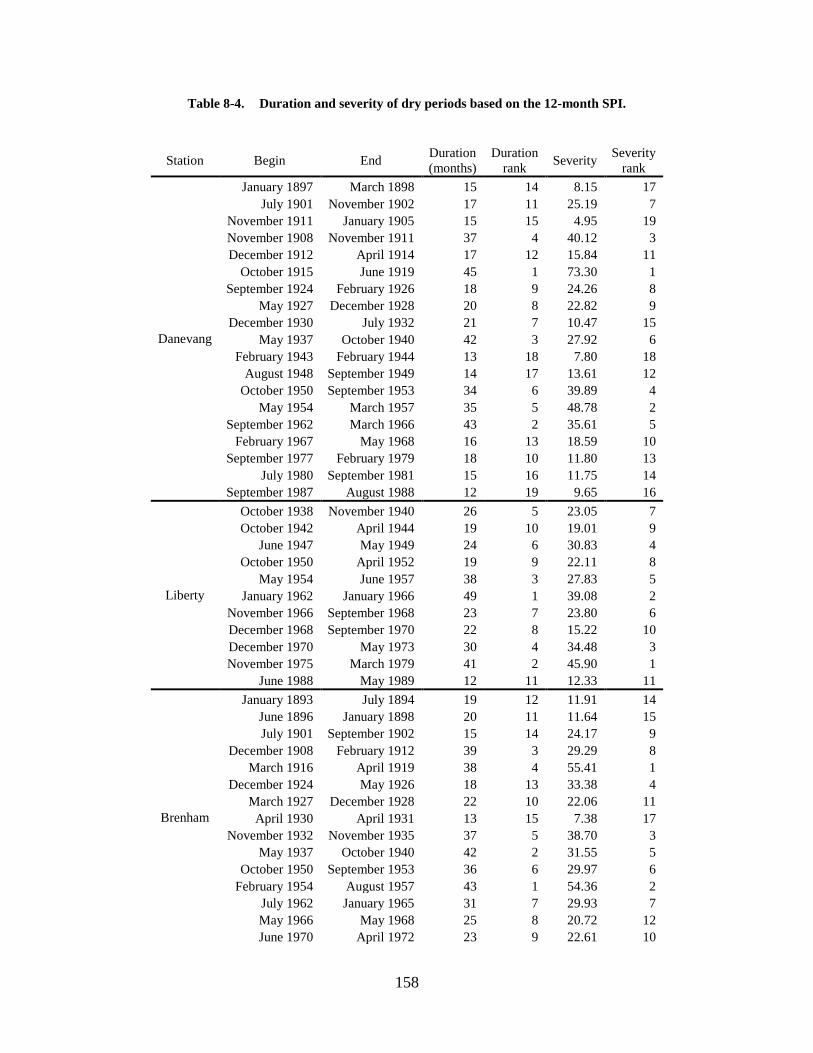
158

Table 8-4. Duration and severity of dry periods based on the 12-month SPI.

Station Begin End Duration

(months) Duration

rank Severity Severity rank

Danevang

January 1897 March 1898 15 14 8.15 17 July 1901 November 1902 17 11 25.19 7

November 1911 January 1905 15 15 4.95 19 November 1908 November 1911 37 4 40.12 3 December 1912 April 1914 17 12 15.84 11

October 1915 June 1919 45 1 73.30 1 September 1924 February 1926 18 9 24.26 8

May 1927 December 1928 20 8 22.82 9 December 1930 July 1932 21 7 10.47 15

May 1937 October 1940 42 3 27.92 6 February 1943 February 1944 13 18 7.80 18

August 1948 September 1949 14 17 13.61 12 October 1950 September 1953 34 6 39.89 4

May 1954 March 1957 35 5 48.78 2 September 1962 March 1966 43 2 35.61 5

February 1967 May 1968 16 13 18.59 10 September 1977 February 1979 18 10 11.80 13

July 1980 September 1981 15 16 11.75 14 September 1987 August 1988 12 19 9.65 16

Liberty

October 1938 November 1940 26 5 23.05 7 October 1942 April 1944 19 10 19.01 9

June 1947 May 1949 24 6 30.83 4 October 1950 April 1952 19 9 22.11 8

May 1954 June 1957 38 3 27.83 5 January 1962 January 1966 49 1 39.08 2

November 1966 September 1968 23 7 23.80 6 December 1968 September 1970 22 8 15.22 10 December 1970 May 1973 30 4 34.48 3 November 1975 March 1979 41 2 45.90 1

June 1988 May 1989 12 11 12.33 11

Brenham

January 1893 July 1894 19 12 11.91 14 June 1896 January 1898 20 11 11.64 15 July 1901 September 1902 15 14 24.17 9

December 1908 February 1912 39 3 29.29 8 March 1916 April 1919 38 4 55.41 1

December 1924 May 1926 18 13 33.38 4 March 1927 December 1928 22 10 22.06 11

April 1930 April 1931 13 15 7.38 17 November 1932 November 1935 37 5 38.70 3

May 1937 October 1940 42 2 31.55 5 October 1950 September 1953 36 6 29.97 6

February 1954 August 1957 43 1 54.36 2 July 1962 January 1965 31 7 29.93 7 May 1966 May 1968 25 8 20.72 12 June 1970 April 1972 23 9 22.61 10

159

Table 8-4. Continued.

Station Begin End Duration (months)

Duration rank Severity Severity

rank

Brenham

June 1970 April 1972 23 9 22.61 10 June 1990 May 1991 12 17 8.28 16

January 1996 December 1996 12 18 7.12 18 October 1999 October 2000 13 16 16.13 13

Luling

December 1864 December 1895 13 15 11.06 16 May 1896 May 1898 25 7 20.73 8

October 1898 March 1900 18 11 17.02 11 April 1904 October 1902 19 9 22.98 7 May 1905 April 1907 12 18 6.17 18

February 1909 November 1912 46 1 41.04 2 October 1915 November 1911 38 4 32.49 5

December 1924 February 1926 15 13 19.41 9 December 1932 November 1934 24 8 14.68 14

July 1937 February 1941 44 2 38.37 4 July 1943 July 1944 13 16 14.69 13

September 1947 March 1949 19 10 18.21 10 April 1954 August 1957 41 3 50.42 1

October 1961 August 1964 35 5 30.82 6 November 1970 December 1971 14 14 10.01 17

May 1984 May 1985 13 17 13.70 15 June 1988 August 1990 27 6 40.65 3

October 1995 January 1997 16 12 16.65 12

Beeville

May 1898 June 1890 50 1 63.85 1 April 1891 November 1892 20 10 19.77 7 June 1896 July 1898 26 7 15.96 9 June 1906 May 1902 12 15 5.88 16

August 1905 November 1908 40 4 57.00 2 September 1910 February 1912 18 12 9.33 14

January 1917 October 1918 22 9 12.42 13 May 1927 September 1928 17 13 15.21 11

December 1928 October 1930 23 8 17.68 8 September 1937 March 1939 19 11 15.53 10

April 1940 June 1942 27 6 27.38 6 July 1943 April 1947 46 2 53.54 4

December 1951 September 1955 46 3 30.85 5 May 1961 April 1962 12 16 9.19 15 June 1972 July 1973 13 14 14.47 12

September 1977 April 1980 32 5 54.51 3

Corpus Christi

September 1890 August 1891 12 17 9.66 15 January 1892 January 1892 13 15 7.73 17 October 1893 April 1895 19 11 17.84 11

July 1895 September 1899 51 2 36.96 5 April 1901 February 1903 23 8 18.42 10 June 1906 May 1912 72 1 75.36 1

November 1915 October 1918 36 6 58.49 2 July 1920 June 1921 12 18 6.56 18

160

Table 8-4. Continued.

Station Begin End Duration (months)

Duration rank Severity Severity

rank

Corpus Christi

August 1924 April 1926 21 10 34.50 6 September 1926 August 1928 24 7 19.51 8

July 1932 December 1933 18 13 10.75 14 April 1950 October 1951 19 12 18.64 9

September 1952 September 1953 13 16 9.44 16 August 1954 August 1957 37 5 44.98 3

October 1961 July 1965 46 3 42.94 4 September 1974 June 1976 22 9 14.18 13

February 1988 May 1991 40 4 32.64 7 June 2000 July 2001 14 14 14.81 12

Encinal

May 1927 September 1930 41 1 38.43 2 November 1938 May 1940 19 6 21.28 5

April 1943 April 1944 13 10 7.33 10 May 1945 August 1946 16 9 9.13 9 May 1951 September 1953 29 4 30.11 4

April 1955 October 1957 31 3 33.75 3 November 1961 August 1964 34 2 40.93 1 September 1968 February 1970 18 7 13.65 7 December 1970 April 1972 17 8 10.17 8 November 1973 June 1975 20 5 15.18 6

Rio Grande

City

March 1952 September 1953 19 4 16.52 4 April 1955 December 1957 33 1 26.32 1

September 1959 November 1960 15 6 14.03 5 December 1961 March 1964 28 2 21.98 2 September 1977 August 1979 24 3 19.94 3

October 1979 April 1981 19 5 11.25 6 SPI = Standardized Precipitation Index

occurred between February 1954 and August 1957 and lasted 43 months (Table 8-4; Figure 8-3). This is also the second most severe event for this station. The most severe event occurred between March 1916 and April of 1919 and lasted 38 months.

The Luling station (Caldwell County) (Figures 8-1 and 8-3) shows 18 events identified that have a median duration of 19 months (Table 8-4). The longest event lasted 46 months, between February 1909 and November 1912. This is also the second most severe event. The most severe event was between April 1954 and August 1957 and ranks as the third longest event.

The Beeville station (Bee County) (Figures 8-1 and 8-3) has 16 identified events (Table 8-4), with a median length of 23 months. The longest duration and most severe event occurred between May 1898 and June 1890, lasting 50 months.

The Corpus Christi station (Nueces County) (Figures 8-1 and 8-3) shows 18 events with a median duration of 22 months (Table 8-4). The longest duration and most severe event at this station occurred between June 1906 and May 1912 and lasted 72 months. The next longest event lasted 51 months, from July 1895 to September 1899. The second most severe event occurred between November 1915 and October 1918, lasting for 36 months.

161

Figure 8-3. Standardized Precipitation Index graphs.

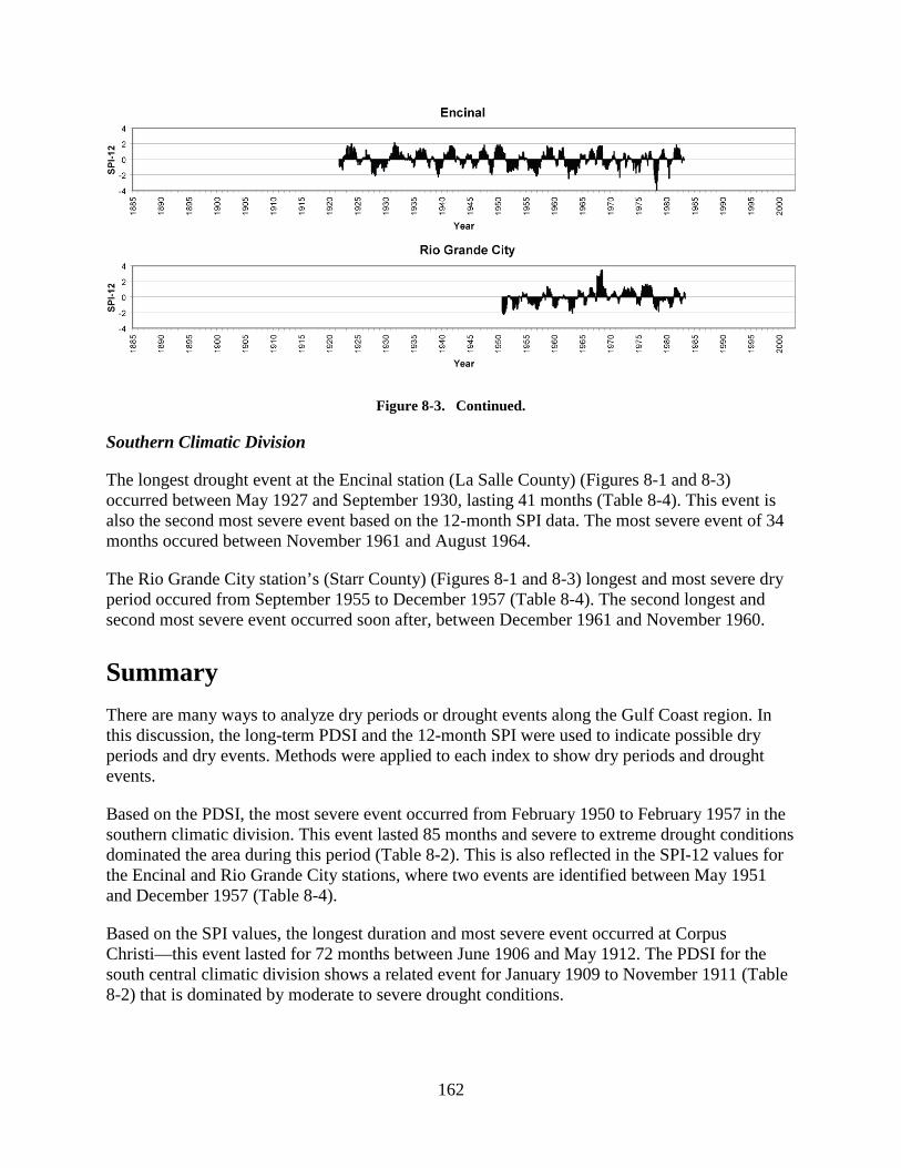
162

Figure 8-3. Continued.

Southern Climatic Division

The longest drought event at the Encinal station (La Salle County) (Figures 8-1 and 8-3) occurred between May 1927 and September 1930, lasting 41 months (Table 8-4). This event is also the second most severe event based on the 12-month SPI data. The most severe event of 34 months occured between November 1961 and August 1964.

The Rio Grande City station’s (Starr County) (Figures 8-1 and 8-3) longest and most severe dry period occured from September 1955 to December 1957 (Table 8-4). The second longest and second most severe event occurred soon after, between December 1961 and November 1960.

Summary There are many ways to analyze dry periods or drought events along the Gulf Coast region. In this discussion, the long-term PDSI and the 12-month SPI were used to indicate possible dry periods and dry events. Methods were applied to each index to show dry periods and drought events.

Based on the PDSI, the most severe event occurred from February 1950 to February 1957 in the southern climatic division. This event lasted 85 months and severe to extreme drought conditions dominated the area during this period (Table 8-2). This is also reflected in the SPI-12 values for the Encinal and Rio Grande City stations, where two events are identified between May 1951 and December 1957 (Table 8-4).

Based on the SPI values, the longest duration and most severe event occurred at Corpus Christi—this event lasted for 72 months between June 1906 and May 1912. The PDSI for the south central climatic division shows a related event for January 1909 to November 1911 (Table 8-2) that is dominated by moderate to severe drought conditions.

163

Dry periods and drought events are common throughout the Gulf Coast region. They can occur every 5 to 6 years and have typical durations of 18 to 24 months.

References d Ó, A., 2005, Regional drought analysis and mitigation using the SPI: International Commission

on Irrigation and Drainage, 21st European Regional Conference proceedings, 9 p.

Edwards, D. C., and McKee, T. B., 1997, Characteristics of 20th century drought in the United States at multiple time scales: Department of Atmospheric Science Colorado State University, 155 p.

Hisdal, H., and Tallaksen, L. M., eds., 2000, Drought event definition: Assessment of the regional impact of droughts in Europe Technical Report No. 6, University of Oslo, Oslo, Norway, 41 p.

Larkin, T. J., and Bomar, G. W., 1983, Climatic atlas of Texas: Texas Department of Water Resources, 152 p.

McKee, T. B., Doesken, N. J., and Kleist, J., 1993, The relationship of drought frequency and duration to time scales: Preprints, 8th Conference on Applied Climatology, p. 179–184.

NCDC, 2005, Time bias corrected divisional temperature-precipitation-drought index (TD-9640): National Climatic Data Center, National Atmospheric and Oceanographic Administration.

NCDC, 2002, Monthly station normals of temperature, precipitation, and heating and cooling degree days 1971-2000: National Climatic Data Center, National Atmospheric and Oceanographic Administration, 88 p.

NCDC, 1983, Statewide average climatic history, Texas 1888-1982: National Climatic Data Center, National Atmospheric and Oceanographic Administration, 39 p.

National Drought Mitigation Center, 2005, SP SPI 6 [computer program].

Palmer, W. C., 1965, Meteorological drought: U.S. Weather Bureau Research Paper No. 45, 58 p.

Texas Drought Preparedness Council, 2005, State of Texas drought preparedness plan: Texas Department of Public Safety, Division of Emergency Management, 24 p.

Williams, C. N., Jr., Menne, M. J., Vose, R. S., and Easterling, D. R., 2005, United States historical climatology network monthly temperature and precipitation data: Oak Ridge National Laboratory/Carbon Dioxide Information Analysis Center 118, NDP-019, Carbon Dioxide Information Analysis Center, Oak Ridge National Laboratory, U.S. Department of Energy, Oak Ridge, Tennessee.

164

This page intentionally blank.

165

Chapter 9

The Impact of Groundwater Flows on Estuaries John A. Breier1

Introduction Direct groundwater discharge to the coastal ocean occurs as submarine seeps and occasionally springs. These discharges occur most frequently along or near the shoreline but are also known to occur quite far offshore on the continental shelf (Moore, 1999; Karpen and others, 2004). These discharges (Figure 9-1) are largely unseen and difficult to quantify because their specific discharge rates are typically low (for example, 1–27 cm per day) (Burnett and others, 2003). Consequently this submarine component of the hydrologic cycle has received historically little attention. However, recent concerns about coastal water quality have prompted increased interest in characterizing and quantifying this submarine groundwater discharge (SGD) and its biogeochemical implications (Moore, 1999). Numerous studies based on direct and indirect measurements have now provided evidence that the exchange of water between coastal sediments and surface waters can be a substantial fraction of surface freshwater inflow (for example, Sewell, 1982; Cable and others, 1996; Moore, 1997; Charette and others, 2001). Because the seepage areas involved are large, the total discharge can be high even where the specific discharge rates are low (Burnett and others, 2003). The chemical implications are even more significant because groundwater is typically enriched relative to surface water in many dissolved constituents such as nutrients and metals. Though our understanding of these processes is still incomplete, there is already evidence that these chemical and water fluxes may have important ecological consequences. The following is a review of our current state of understanding of the scope and processes involved in SGD; the methods used to investigate SGD, their current limitations, and some of the ways researchers are trying to overcome them; and the chemical and ecological consequences of SGD on estuaries.

Submarine Groundwater Discharge SGD refers to the mixture of terrestrial advecting groundwater and saline recirculated seawater that discharges directly to the coastal ocean (Moore, 1999). Estimates of the terrestrial advecting fraction of SGD are between six and ten percent of surface water inputs; however, total SGD discharge can be much greater due to the recirculated seawater component (Burnett and others, 2003). While municipal water managers have historically been interested in the discharge of

1 The University of Texas at Austin—Marine Science Institute

166

Figure 9-1. Though in many ways difficult to observe, submarine groundwater discharge can be imaged by a) infrared photography (image provided by Ann Mulligan and Matt Charette) and b) ‘schlieren’ photographic techniques sensitive to the density differences between saline and fresh or brackish groundwater (reprinted from Karpen and others, 2004, copyright 2003, with permission from Elsevier). In this a) thermal infrared aerial photograph of a tidal pond near Waquoit Bay, MA, the cooler (lighter) groundwater discharge can be seen mixing with the warmer (darker) bay water (Mulligan and Charette 2005). In b) a specially designed underwater ‘schlieren’ photographic system images submarine seepage several kilometers offshore in the Baltic Sea (Karpen and others, 2004).

terrestrial groundwater to the ocean, the total SGD must be quantified when considering the biogeochemical effects on estuaries.

A variety of driving forces are involved in controlling the discharge of this terrestrial and seawater mixture (see Burnett and others, 2003 for a detailed review). The terrestrial hydraulic gradient and the permeability and thickness of aquifer materials and bay bottom sediments control the discharge and spatial heterogeneity of both terrestrial and entrained recirculated seawater. Tidal and wind driven changes in sea level influence the hydraulic gradient as well as induce wave and tidal pumping of bay bottom and shoreline sediments (Burnett and others, 2003). Density differences between fresh groundwater and more saline or even hypersaline surface waters in salt marshes and tidal flats can result in buoyant forces and density driven convection (Simmons and others, 1991). A consequence of this complex mixture of fluids and driving forces is that SGD varies temporally and spatially even at relatively small scales, making it difficult to locate areas of significant submarine discharge difficult and relate the results of large and small scale SGD investigations (Breier and others, in review).

Quantifying Submarine Groundwater Discharge There are three basic approaches to quantifying SGD including hydrogeologic modeling, direct seepage measurements, and chemical tracer mixing models (Burnett and Dulaiova, 2003; Oberdorfer, 2003). However, these methods do not all measure the same components of SGD and are not necessarily directly comparable. Hydrogeologic modeling has typically been used to

167

estimate the advecting terrestrial component of SGD. More recently, variable density groundwater transport algorithms have been used to include the recirculated seawater component (Oberdorfer, 2003). Seepage meters are used in relatively small areas and are especially useful in areas where SGD is already known to occur. Seepage meter measurements reflect total SGD; if discharge salinity is also measured, then the advecting groundwater and recirculated seawater components can be also be estimated. Chemical tracers are the most common approach because they can be used to estimate SGD to large areas such as entire bays or regions. Chemical tracer estimates generally reflect some combination of advecting groundwater and recirculated seawater discharge, depending on the specific tracer.

Estimates of total SGD are theoretically possible if the nearshore hydraulic gradient and sediment permeability are well known. In practice, obtaining the necessary data in other than the first few meters of sediment requires extensive drilling, geophysical surveying, or extrapolation of sparse data. Langevin (2001) used the U.S. Geological Survey’s SEAWAT variable density groundwater transport code to model total SGD to Biscayne Bay, Florida, with mixed results. Both regional three-dimensional and local-scale two-dimensional vertical models were developed assuming steady-state conditions and homogeneous aquifer characteristics. While the variable density transport code was capable of estimating both the advecting groundwater and recirculated seawater components of SGD, it was not able to accurately simulate the groundwater salinities beneath Biscayne Bay as observed in monitoring wells. Additionally, surface aquifer recharge rate and the terrestrial boundary groundwater flux must be estimated and the aquifer hydraulic parameters adjusted to calibrate the modeled water-table elevations to monitoring well levels (Langevin, 2001). Similar boundary conditions and calibrations are necessary in most if not all hydrogeologic models and introduce considerable uncertainty in their results.

SGD can be directly measured at the sediment/water interface using a seepage meter (for example, Cable and others, 1997; Michael and others, 2003) which collects seepage through a small area of the sediment surface. In addition to being labor intensive, seepage meters have an inherent bias which underestimates discharge due to the increased hydraulic friction associated with the meter (Cable and others, 1997). Further, because SGD is frequently heterogeneous, seepage meter results exhibit large variability (Michael and others, 2003) and only limited extrapolation of results to larger areas is possible.

Chemical tracers such as radium, radon, and methane provide an integrated spatial signal allowing quantification of SGD throughout entire bay systems (for example, Rama and Moore, 1996; Krest and others, 1999; Charette and others, 2003; Breier and others, 2004). The ideal chemical tracer of SGD is a dissolved constituent which (1) exhibits a substantial enrichment in groundwater relative to other potential end-member waters (for example, seawater, river water, rain, and runoff) and (2) behaves conservatively within the coastal zone (Charette and others, 2001). Radon is perhaps closest to the ideal; it is highly enriched in groundwater, as a noble gas exhibits very conservative behavior, and is relatively straightforward to measure (Cable and others, 1996; Burnet and Dulaiova, 2003). Radium isotopes are also powerful tracers of SGD because they behave conservatively in brackish and marine waters and are enriched in groundwater (Krest and others, 1999). They also provide a means of estimating bay residence time and tidal transport which is essential to properly modeling tracer mixing within a study area (Charette and others, 2001). Methane is a product of anaerobic decay and is found in high concentrations in anoxic groundwaters with sufficient organic matter for methanogenesis but is

168

subject to microbial uptake and production and is not strictly conservative (Bugna and others, 1996). Regardless of the trace, SGD is estimated from a mixing model for the chemical species in question (for example, Breier and Edmonds, in review).

While the techniques just mentioned can provide valuable data, they can also involve substantial uncertainty. In particular, determining the spatial distribution of SGD in a study area can be very challenging. While natural chemical tracers are useful at estimating total discharge to an area, they cannot be used to pinpoint the source of discharge because water column mixing weakens and spatially integrates the signal. Conversely, while direct measurements with seepage meters can be used to measure discharge at a point, they do not capture spatial variation in the system and can miss significant localized discharges altogether. In fact, only in a few well studied areas is the spatial distribution of SGD understood at a scale approaching that at which organisms experience its effects. This has hampered attempts at studying the ecological consequences of SGD. Recently, the use of simultaneous geochemical and geophysical surveying (Figure 9-2) and thermal infrared aerial photography have demonstrated that there are ways to acquire more detailed spatial data on SGD (Bratton and others, 2004; Breier and others, in review; Mulligan and Charette, 2005). Data from techniques will help plan future field studies which more directly test the biogeochemical and ecological hypotheses concerning SGD.

Chemical and Ecological Consequences of Submarine Groundwater Discharge Johannes (1980) was one of the first to seriously discuss groundwater as a potential pathway for nutrients to coastal estuaries. Because groundwater is often enriched in natural and anthropogenic nutrients, SGD may be ecologically important even where discharge rates are small compared to surface water inputs. If SGD does represent an important control on estuarine salinity and chemical cycling, particularly nutrients, then it is reasonable to suspect that SGD dynamics and distribution may also affect ecosystem processes (Johannes, 1980). Two widely expressed concerns are that (1) fluctuations in SGD rates are related to the initiation of nuisance algal blooms (Sewell, 1982; Laroche and others, 1997) and (2) anthropogenic increases in groundwater nutrient concentrations are partially responsible for the increasing eutrophication of coastal waters (for example, Johannes, 1980; Laroche and others, 1997).

Perhaps the most widely discussed hypothesis related to SGD is that changes in the associated nutrient flux may initiate algal blooms. Evidence supporting this comes from a study by Laroche and others (1997) of 11 years of well levels, coastal salinities, nutrient concentrations, and cell counts of the brown tide species Aureococcus anophagefferens in Peconic Bay, Long Island. Laroche and others (1997) showed that bloom intensity was inversely proportional to well levels and directly proportional to bay salinities. However, bay salinity does not itself appear to be the direct initiator of A. anophagefferens blooms. The salinity of Peconic Bay during the study years was within the optimal growth range of A. anophagefferens growth 98 percent of the time. Instead, high bay salinity is a result of low SGD, and when SGD is low, the ratio of organic to inorganic nitrogen in the bay increases. A. anophagefferens is believed to have a competitive advantage in utilizing organic nitrogen compared to other algal species and increased inorganic nitrogen has been shown to inhibit A. anophagefferens growth. Local groundwater in the Peconic

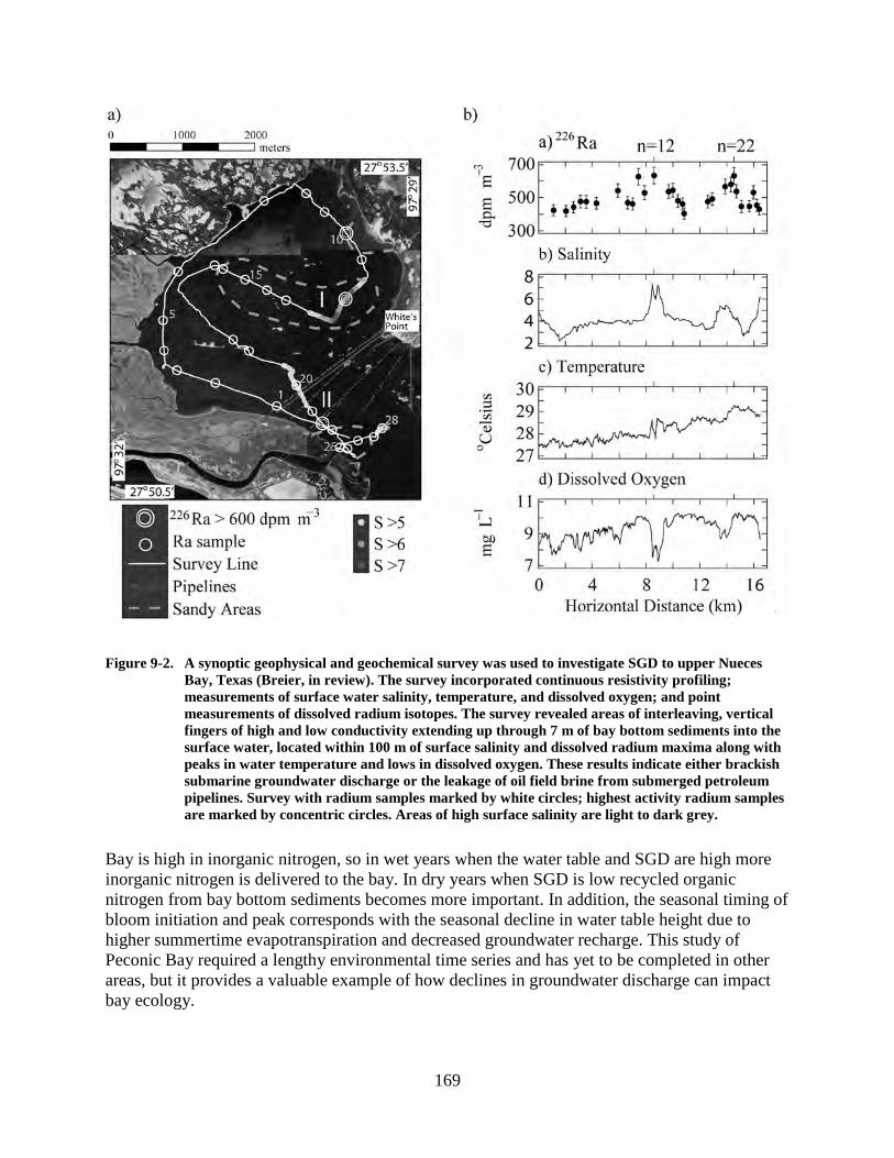
169

Figure 9-2. A synoptic geophysical and geochemical survey was used to investigate SGD to upper Nueces Bay, Texas (Breier, in review). The survey incorporated continuous resistivity profiling; measurements of surface water salinity, temperature, and dissolved oxygen; and point measurements of dissolved radium isotopes. The survey revealed areas of interleaving, vertical fingers of high and low conductivity extending up through 7 m of bay bottom sediments into the surface water, located within 100 m of surface salinity and dissolved radium maxima along with peaks in water temperature and lows in dissolved oxygen. These results indicate either brackish submarine groundwater discharge or the leakage of oil field brine from submerged petroleum pipelines. Survey with radium samples marked by white circles; highest activity radium samples are marked by concentric circles. Areas of high surface salinity are light to dark grey.

Bay is high in inorganic nitrogen, so in wet years when the water table and SGD are high more inorganic nitrogen is delivered to the bay. In dry years when SGD is low recycled organic nitrogen from bay bottom sediments becomes more important. In addition, the seasonal timing of bloom initiation and peak corresponds with the seasonal decline in water table height due to higher summertime evapotranspiration and decreased groundwater recharge. This study of Peconic Bay required a lengthy environmental time series and has yet to be completed in other areas, but it provides a valuable example of how declines in groundwater discharge can impact bay ecology.

170

Increases in SGD and/or the associated nitrogen flux can also impact bay and coastal ecology. Increases in SGD-delivered inorganic nitrogen can stimulate aquatic plant growth. Maier and Pregnall (1990) showed that the growth of the eelgrass Zostera Marina and the macroalgae Sargassum filipendula and Enteromorpha intestinalis are all stimulated by nitrate enrichment. Typically eelgrass utilizes ammonium for growth; however, in sandy beaches around Woods Hole, Massachusetts, eelgrass growing in areas of SGD were shown to have elevated nitrate reductase enzyme activity, indicating that they were utilizing SGD-derived nitrate for growth. The macroalgal species growing in the same area exhibited even higher nitrate reductase activity, indicating that they are more successful at utilizing nitrate for growth. Maier and Pregnall (1990) suggest that at certain levels groundwater nitrate flux may influence and stimulate the growth of marine plants like the eelgrass Z. Marina, but when the groundwater nitrate flux is higher the growth of macroalgae takes over and can ultimately smother the bottom plants. A similar process has been observed in Jamaican and Floridian coral reefs where an increase in dissolved inorganic nitrogen in near bottom waters has stimulated the growth of epilithic macroalgae at the expense of the corals on which they grow (Lapointe, 1997). This process has been going on for some time and in the case of the Jamaican coral reefs the macroalgae now dominates. The elevated nitrate and low salinity in near bottom waters of these reefs indicates that the nitrate is being delivered by groundwater. In addition, analysis of macroalgae tissue shows elevated d15N which suggests that the nitrate is ultimately coming from groundwater contaminated by wastewater (Lapointe, 1997).

SGD may also influence estuarine ecology in ways other than modifying nutrient supply. First, the spatial distribution of SGD within an embayment may create environmental refugia for some organisms (for example, Nielsen and Lisle, 1994). Freshwater fish such as steelhead trout use pools influenced by groundwater discharge as thermal refuge (Nielsen and Lisle, 1994). Aquatic biota may also use such areas to escape chronic hypoxia particularly in times of drought or low river discharge (Magoulick and Kobza, 2003). Second, since the dissolved O2 concentration of groundwater varies, suboxic or anoxic SGD may be a mechanism for the remobilization of redox sensitive transition metals in bay sediments (Liu and others, 2001).

Conclusions Evidence of significant submarine groundwater fluxes has been growing in recent years. SGD investigations to date have largely focused on locating and quantifying the amounts of SGD to different areas. Limited but provocative evidence of the ecological effects of these discharges on harmful algal bloom initiation and eutrophication have already been found. Other ecological impacts are suspected but remain to be tested. Methods and techniques are just now reaching the point that we can identify and investigate these fluxes on the very small scales at which organisms experience them.

References Bratton, J. F., Crusiu, J. F., Meunier, J. K., Spruill, T. B., and Wrege, B. M., 2004, Use of

continuous resistivity profiling to detect low-salinity ground water beneath the Upper Neuse

171

River Estuary, North Carolina: EOS Transactions, American Geophysical Union, v. 85, no. 47, Fall Meeting Supplement, Abstract H24A-04.

Breier, J. A., and Edmonds, H. N., in review, High 226Ra and 228Ra activities in Nueces Bay, Texas indicate submarine saline discharges: submitted to Marine Chemistry.

Breier, J. A., Breier, C. F., and Edmonds, H. N., in review, Detecting submarine groundwater discharge with synoptic surveys of sediment resistivity, radium, and salinity: submitted to Geophysical Research Letters.

Breier, J. A., Edmonds, H. N., and Villareal, T. A., 2004, Submarine groundwater discharge and associated nutrient fluxes to the Corpus Christi Bay system: Texas Water Development Board Contract Report 2002-483-416, 50 p.

Bugna, G. C., Chanton, J. P., Cable, J. E., Burnett, W. C., and Cable, P. H., 1996, The importance of groundwater discharge to the methane budgets of nearshore and continental shelf waters of the northeastern Gulf of Mexico: Geochimica et Cosmochimica Acta, v. 60, p. 4735–4746.

Burnett, W. C., Bokuniewicz, H., Huettel, M., Moore, W. S., and Taniguchi, M., 2003, Groundwater and pore water inputs to the coastal zone: Biogeochemistry, v. 66, p. 3–33.

Burnett, W. C., and Dulaiova, H., 2003, Estimating the dynamics of groundwater input into the coastal zone via continuous radon-222 measurements: Journal of Environmental Radioactivity, v. 69, p. 21–35.

Cable, J. E., Bugna, G. C., Burnett, W. C., and Chanton, J. P., 1996, Application of 222Rn and CH4 for assessment of groundwater discharge to the coastal ocean: Limnology and Oceanography, v. 41, p. 1347–1353.

Cable, J. E., Burnett, W. C., and Chanton, J. P., 1997, Magnitude and variation of groundwater seepage along a Florida marine shoreline: Limnology and Oceanography, v. 38, p. 189–205.

Charette, M. A., Buesseler, K. O., and Andrews, J. E., 2001, Utility of radium isotopes for evaluating the input and transport of groundwater-derived nitrogen to a Cape Cod estuary: Limnology and Oceanography, v. 46, p. 465–470.

Charette, M. A., Splivallo, R., Herbold, C., Bollinger, M. S., and Moore, W. S., 2003, Salt marsh submarine groundwater discharge as traced by radium isotopes: Marine Chemistry, v. 84, p. 113–121.

Johannes, R. E., 1980, The ecological significance of the submarine discharge of groundwater: Marine Ecology Progress Series, v. 3, p. 365–373.

Karpen, V., Thomsen, L., and Suess, E., 2004, A new 'schlieren' technique application for fluid flow visualization at cold seep sites: Marine Geology, v. 204, p. 145–159.

Krest, J. M., Moore, W. S., and Rama, 1999, 226Ra and 228Ra in the mixing zones of the Mississippi and Atchafalaya Rivers—Indicators of groundwater input: Marine Chemistry, v. 64, no. 3, p. 129–152.

Langevin, C. D., 2001, Simulation of ground-water discharge to Biscayne Bay, southeastern Florida: Water Resources Investigation Report 00-4251, U.S. Geological Survey, 127 p.

172

Lapointe, B., 1997, Nutrient thresholds for bottom-up control of macroalgal blooms on coral reefs in Jamaica and southeast Florida: Limnology and Oceanography v. 42, p. 1119–1131.

Laroche, J., Nuzzi, R., Waters, R., Wyman, K., Falkowski, P. G., and Wallace, D. W. R., 1997, Brown tide blooms in Long Island's coastal waters linked to interannual variability in groundwater flow: Global Change Biology, v. 3, p. 397–410.

Liu, C., Jay, J. A., Ika, R., Shine, J. P., and Ford, T. E., 2001, Capping efficiency for metal-contaminated marine sediment under conditions of submarine groundwater discharge: Environmental Science and Technology, v. 35, p. 2334–2340.

Magoulick, D. D. and Kobza, R. M., 2003, The roles of refugia for fishes during drought—A review and synthesis: Freshwater Biology, v. 48, p. 1186–1198.

Maier, C. M. and Pregnall, A. M., 1990, Increased macrophyte nitrate reductase activity as a consequence of groundwater input of nitrate through sandy beaches: Marine Biology, v. 107, p. 263–271.

Michael, H. A., Lubetsky, J. S., and Harvey, C. F., 2003, Characterizing submarine groundwater discharge—A seepage meter study in Waquoit Bay, Massachusetts: Geophysical Research Letters, v. 30, p. 1–4.

Moore, W. S., 1997, High fluxes of radium and barium from the mouth of the Ganges-Brahmaputra River during low river discharge suggest a large groundwater source: Earth and Planetary Science Letters, 150, p. 141–150.

Moore, W. S., 1999, The subterranean estuary—A reaction zone of ground water and sea water: Marine Chemistry, v. 65, no. 1-2, p. 111–125.

Mulligan, A., and Charette, M., 2005, Intercomparison of submarine groundwater discharge estimates from a sandy unconfined aquifer: The Geological Society of America, v. 37, Fall Meeting, Abstracts with Programs, Abstract 191-5.

Nielsen, J. L., and Lisle, T. E., 1994, Thermally stratified pools and their use by steelhead in Northern California streams: Transactions of the American Fisheries Society, v. 123, p. 613–626.

Oberdorfer, J. A., 2003, Hydrogeologic modeling of submarine groundwater discharge—Comparison to other quantitative methods: Biogeochemistry, v. 66, p. 159–169.

Rama, and Moore, W. S., 1996, Using the radium quartet for evaluating groundwater input and water exchange in salt marshes: Geochimica et Cosmochimica Acta, v. 60, p. 4645–4652.

Sewell, P. L., 1982, Urban groundwater as a possible nutrient source for an estuarine benthic algal bloom: Estuarine Coastal Shelf Science, v. 13, p. 569–576.

Simmons, C. T., Fenstemaker, T. R., and Sharp, J. M., Jr., 1991, Variable-density groundwater flow and solute transport in heterogeneous porous media—Approaches, resolutions and future challenges: Journal of Contaminant Hydrology, v. 52, p. 245–275.

173

Chapter 10

Groundwater Models of the Gulf Coast Aquifer of Texas Ali H. Chowdhury, Ph.D., P.G.1, and Robert E. Mace, Ph.D., P.G.1

Introduction

Models of groundwater flow are useful for better understanding aquifers and, ultimately, for better managing groundwater resources. Groundwater models allow hydrogeologists and engineers to bring available information and estimates on aquifers together to see how this information interacts with itself. Once a model is developed, it can be used to predict how water levels in the aquifer might respond to pumping and drought. For the Gulf Coast area, land subsidence, where the sediments compress in response to pumping groundwater, is another concern that groundwater models can be used to predict.

Groundwater modeling in Texas has had a long history (Mace, 2001) that starts with an electric analog model developed for the Gulf Coast aquifer in the Houston area in 1965 and continues today as our understanding of the aquifer and the development of modeling tools improve. The Texas Legislature approved funding for the Groundwater Availability Modeling (GAM) program at the Texas Water Development Board (TWDB) in recognition of the importance of obtaining accurate estimations of groundwater availability. The goal of the GAM program is to provide useful and timely information on groundwater availability to the citizens of Texas. In order to achieve this, the TWDB developed or acquired models of all the major aquifers in Texas, including the Gulf Coast aquifer. The TWDB continues work to develop groundwater models for the minor aquifers of Texas.

Groundwater models are useful tools for entities charged with managing groundwater resources. Groundwater in the Gulf Coast aquifer of Texas is managed by several groundwater conservation districts and two subsidence districts (Figure 10-1). Outside the districts, groundwater is managed by the rule of capture (Mace and others, 2004). With the passage of House Bill 1763 in 2005, groundwater conservation districts in each groundwater management area are required to meet to determine the desired future conditions for each of their aquifers. The TWDB is then charged with providing estimates of managed available groundwater to groundwater conservation districts and regional water planning groups for use in their plans. It is likely that

1 Texas Water Development Board

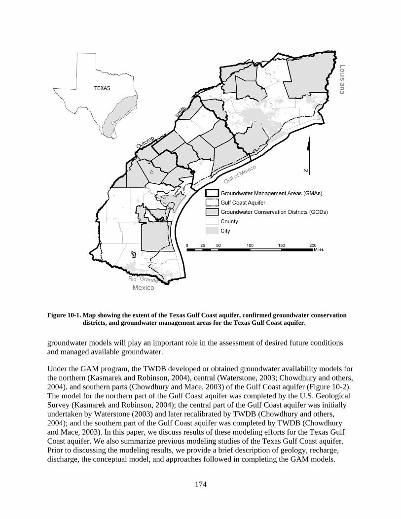
174

Figure 10-1. Map showing the extent of the Texas Gulf Coast aquifer, confirmed groundwater conservation districts, and groundwater management areas for the Texas Gulf Coast aquifer.

groundwater models will play an important role in the assessment of desired future conditions and managed available groundwater.

Under the GAM program, the TWDB developed or obtained groundwater availability models for the northern (Kasmarek and Robinson, 2004), central (Waterstone, 2003; Chowdhury and others, 2004), and southern parts (Chowdhury and Mace, 2003) of the Gulf Coast aquifer (Figure 10-2). The model for the northern part of the Gulf Coast aquifer was completed by the U.S. Geological Survey (Kasmarek and Robinson, 2004); the central part of the Gulf Coast aquifer was initially undertaken by Waterstone (2003) and later recalibrated by TWDB (Chowdhury and others, 2004); and the southern part of the Gulf Coast aquifer was completed by TWDB (Chowdhury and Mace, 2003). In this paper, we discuss results of these modeling efforts for the Texas Gulf Coast aquifer. We also summarize previous modeling studies of the Texas Gulf Coast aquifer. Prior to discussing the modeling results, we provide a brief description of geology, recharge, discharge, the conceptual model, and approaches followed in completing the GAM models.

175

Figure 10-2. Map showing groundwater model areas for the northern, central, and southern parts of the Gulf Coast aquifer. Types of model boundaries for each model area are also indicated.

Following this, we discuss model calibration results for steady-state and transient conditions and present the amount of groundwater flowing through the aquifer in respective model areas.

Past and Present Models of the Gulf Coast of Texas

Several state and federal agencies have conducted studies on the geology and hydrogeology of the Texas Gulf Coast aquifer (for example, Wood and Gabrysch, 1965; Jorgensen, 1975; Baker and Wall, 1976; Baker, 1979; Meyer and Carr, 1979; Carr and others, 1985; Groschen, 1985; Baker, 1986; Ryder, 1988; Dutton and Richter, 1990; McCoy, 1990; Hay, 1999; Harden and Associates, 2002; Kasmarek and Strom, 2002). Most of these studies involved characterizing the

176

hydrogeology of the aquifers in support of groundwater model development with emphasis on major pumping centers in the Houston area.

Modeling efforts in the Gulf Coast aquifer of Texas have evolved from the construction of simplistic electric-analog model covering a small area to more complex numerical models covering large areas and multiple aquifers (for example, Wood and Gabrysch, 1965; Jorgensen, 1975; Meyer and Carr, 1979). With the advancement of computer technology, more complex, regional, groundwater flow models were constructed for the Gulf Coast aquifer (Carr and others, 1985; Groschen, 1985; Ryder, 1988; Hay, 1999; Harden and Associates, 2002). We present a brief description of these models below.

Wood and Gabrysch (1965) developed an electric-analog model containing the Evangeline aquifer and part of the Chicot aquifer (Alta Loma Sand) to simulate transmissivities and storativities over an area covering about 5,000 square miles in the northern part of the Gulf Coast aquifer. The model used five stress periods to simulate drawdown from 1890 to 1960 in response to groundwater pumping. The model was limited by its inability to simultaneously stress the aquifers and its inability to reproduce effects of groundwater pumping (Kasmarek and Robinson, 2004).

Jorgensen (1975) used an updated electric analog model and allowed vertical communication between the Chicot and Evangeline aquifers and expulsion of water into the aquifer from clay compaction. However, the model was unable to reproduce land-surface subsidence.

Meyer and Carr (1979) used a finite-difference method to simulate groundwater flow in the Chicot and the Evangeline aquifers with model boundaries extended out from major pumping centers. Their model consisted of five layers: layer 1 consisted of total thickness of sand beds in the Evangeline aquifer; layer 2 consisted of clay thickness from the centerline of the Chicot and the centerline of the Evangeline aquifers; layer 3 consisted of the Alta Loma Sand or the total sand thickness of the Chicot aquifer; layer 4 included clay thickness from between the land surface and the centerline of the Chicot aquifer; and layer 5 represented the top layer as an upper boundary to allow infiltration of recharge and irrigation return flow.

Carr and others (1985) constructed and calibrated a numerical groundwater flow model of the Chicot and Evangeline aquifers extending from the Texas-Louisiana border to the northern half of Jim Hogg, Brooks, and Kenedy counties. This model had four layers that incorporated hydraulic properties of distinct horizons of clay and sand beds of the Chicot and the Evangeline aquifers. Vertical leakage through clays into the Chicot aquifer was found to be significant in the upper part of the Gulf Coast aquifer, but it decreased considerably in the southern portions of the Lower Rio Grande Valley. Model calibration was most sensitive to transmissivity and unconfined storage.

Groschen (1985) constructed a groundwater flow and solute transport model to assess saline water movement in the Evangeline aquifer using projected pumping through 2020. The model covered an area of 4,680 square miles from San Patricio County in the north to northern parts of Jim Hogg, Brooks, and Kenedy counties to the south. The model included the Chicot, Evangeline, and Jasper aquifers and the Burkeville confining system; had 38 square grids with each cell 2 miles long; and used constant heads in the outcrop to simulate recharge. The model

177

suggested that the saline water-fresh water interface would not be affected by increased pumping and that most of the salinity in the Evangeline aquifer was due to leakage from the overlying Chicot aquifer.

Ryder (1988) developed a three-dimensional variable-density model covering the entire Texas Gulf Coast and parts of Louisiana and Mexico. All fourteen geologic units contained within the Gulf Coast and the Carrizo-Wilcox aquifers above the geo-pressure zone (fluid pressure in excess of hydrostatic pressure) were included in the model to simulate flow under predevelopment conditions. Recharge was simulated using constant heads at the outcrop representing water levels in the top 100 feet of the aquifer. The model did a better job of matching the water levels in the outcrop than in the deeper parts of the aquifers.

Hay (1999) developed a three-dimensional steady-state model for Region N as part of regional water planning in Texas. This model included the Chicot, Evangeline, and Jasper aquifers and the Burkeville Confining System. Constant heads were assigned in the outcrop to simulate recharge into the aquifers.

Harden and Associates (2002) developed a model covering an area of about 90 miles by 60 miles to evaluate water availability and drawdown in the Rio Grande alluvium near Brownsville. Rather than using actual structure surfaces for the model layers, the model used average thickness of the Rio Grande alluvium and included four layers based on levels of groundwater production (a surface zone, a primary zone, a separation zone, and a secondary zone).

Kasmarek and Strom (2002) developed a model for simulating groundwater flow and land- surface subsidence with a focus on Harris and Galveston counties. The model consisted of three layers: layer 1 represents the water table using a specified head, layer 2 represents the Chicot aquifer, and layer 3 represents the Evangeline aquifer. Groundwater flow simulations were conducted for 1891 through 1996, and 1977 and 1996 water levels were chosen for calibration. Simulation results indicated that about 19 percent of the water in the Chicot aquifer and about 10 percent of the water in the Evangeline aquifer are drawn from clay storage.

As part of the GAM program, TWDB staff and TWDB contractors developed three new regional models of the Gulf Coast of Texas: (1) Kasmarek and Robinson (2004) developed a model of the northern part of the Gulf Coast aquifer in cooperation with TWDB and the Harris-Galveston Subsidence District; (2) Waterstone (2003) and Chowdhury and others (2004) developed a model of the central part of the Gulf Coast aquifer, and (3) Chowdhury and Mace (2003) developed a model of the southern part of the Gulf Coast aquifer. Other modeling work continues in the area, including a model of the central part of the Gulf Coast aquifer by Texas A&M—Kingsville (Venki Uddanmeri, personal communication, 2005) and a model of the Gulf Coast aquifer in the vicinity of the Colorado River by the Lower Colorado River Authority (Steve Young, personal communication, 2005). The focus of this chapter is on the work done for the GAM program.

Hydrogeologic Setting

We adopted Baker's (1979) hydrostratigraphy for the development of the GAMs for the Gulf Coast aquifer because it included: (1) detailed faunal occurrences, lithologies, and electric log

178

signatures along with several cross-sections; (2) hydraulic characteristics of the sediments; and (3) water-level information. From oldest to youngest, the Tertiary rocks have been classified into the Frio Formation, the Anahuac Formation, and the Catahoula Tuff or Sandstone (Early Miocene); the Oakville Sandstone and the Fleming Formation (Mid- to Late-Miocene); the Goliad Sand (Pliocene); the Willis Sand, Bentley Formation, Montgomery Formation, Beaumont Clay (Pleistocene); and alluvium (Holocene) (Baker, 1979).

Excessive groundwater pumping has caused water-level declines in various parts of the Gulf Coast aquifer (Chowdhury and others, 2004; Kasmarek and Robinson, 2004). Major cones of depression occur in Harris-Galveston, Wharton-Jackson-Matagorda, and Kleberg counties, where water levels have historically declined by up to 350, 50, and 200 feet, respectively (Chowdhury and others, 2004; Kasmarek and Robinson, 2004). Excessive pumping of the aquifer caused subsequent land-surface subsidence due to compaction and expulsion of water from the clays contained in the aquifer materials and shale beds (Gabrysch, 1984). For example, in the Houston area, the land surface has subsided up to ten feet locally (Kasmarek and Robinson, 2004).

Groundwater in the Texas Gulf Coast aquifer generally flows from the outcrop areas in the west towards the Gulf of Mexico in the east. Most of the water-level contours parallel the coastline except near major pumping centers where natural flow system is altered and water is diverted toward major cones of depression (Chowdhury and others, this volume). Water levels in wells vary widely depending on their locations with respect to the groundwater flow system. In the unconfined parts of the outcrop, most of the wells respond quickly to precipitation events. In the confined parts of the aquifer away from the outcrop, groundwater movement is slow and water levels in wells do not respond to precipitation, due to the long travel time through the subsurface. Groundwater pumping perhaps is probably the most important control in shaping water-level changes in wells. For example, many wells in the confined parts of the aquifer that record historical decline in water levels display significant recovery over time due to reduction in pumping.

Recharge

Recharge mainly occurs from rainfall that falls on the outcrop areas. Only a small portion of the rainfall reaches the water table. Water also drains into the aquifer from some reaches of the numerous streams that cross the Gulf Coast. In other reaches of the streams, groundwater discharges into streams as baseflow. In addition, major pumping centers that form large cones of depression may capture recharged water that was naturally discharging to local streams, thereby increasing downdip recharge. Recharge through the unconfined, permeable, sandy portions of the Gulf Coast aquifer may be relatively fast, while recharge to the confined portions of the aquifer may be considerably slow. Recharge through the Beaumont Clay that outcrops along the coast is generally small except in areas where valleys have been cut into the formation. Water not evaporated, consumed by plants through transpiration, or drained by streams from surface runoff infiltrates into the subsurface and eventually reaches the water table.

Several investigators have estimated recharge rates for the Gulf Coast aquifer (Groschen, 1985; Ryder, 1988; Dutton and Richter, 1990; Ryder and Ardis, 2002; Kasmarek and Robinson, 2004) (Table 10-1). Recharge rates derived from most of the model simulations are generally similar

179

(Table 10-1). Some variations observed in recharge estimates are probably due to local variations in (1) hydraulic conductivity, (2) rainfall distribution, (3) evapotranspiration, (4) groundwater-surface water interactions, (5) model grid sizes, and (6) surface geology. More importantly, it is notable that recharge rates reported in these studies are for different time periods. Noble and others (1996) estimated a higher recharge rate of about six inches per year using a tritium isotope method. However, this recharge estimate is an upper limit, includes a shallow flow system that locally discharges to streams, and may contribute little or no recharge to the deep regional flow system. Pumping from the aquifer and a subsequent lowering of the water table induced additional recharge in parts of the Gulf Coast aquifer (Ryder and Ardis, 2002; Kasmarek and Robinson, 2004).

Table 10-1. Recharge rates from previous studies of the Gulf Coast aquifer (after Chowdhury and Mace, 2003).

Groschen (1985) 0.06 San Patricio to Jim Hogg counties

Constant head

Ryder (1988) 0 to 6 Texas Gulf Coast Specified head, top layer of the modelDutton and Richter (1990) 0.1 to 0.4 Matagorda and Wharton

countiesHead-dependent flux boundary, top layer of

the modelNoble and others (1996) 6 Harris, Montgomery and

Walker countiesIsotopes

Hay (1999) 0.078 Navidad River to Willacy County

Constant head

Harden and Associates (2001)

0.1 to 0.2 Brownsville and vicinity Used maximum potential recharge (3 inches) and MODFLOW’s River Package

Ryder and Ardis (2002) 0.121-0.252 Texas Gulf Coast Specified head, top layer of the modelKasmarek and Strom (2004) 0.323-0.434 Northern Gulf Coast GAM Specified head, top layer of the model

Chowdhury and Mace (2004) 0.09 to 0.15 Southern Gulf Coast GAM Calibrated recharge as a percent of distributed rainfall

1 = average recharge for the predevelopment model, 2 = average

recharge for 1982

3 = average recharge for 1977, 4 = average recharge for 2000

Source Study Area Recharge MethodRecharge Rate (in/yr)

Discharge

Natural discharge in the Gulf Coast aquifer occurs through springs, evapotranspiration, baseflow, and upward leakage of groundwater from deeper into shallower aquifers. Under pre-development conditions, average discharge across the Gulf Coast aquifer ranges from zero to one inch per year (Ryder and Ardis, 2002). Excessive groundwater pumping in the Gulf Coast aquifer has resulted in a decrease of the discharge area under pumping conditions compared to non-pumping conditions (Dutton and Richter, 1990; Ryder and Ardis, 2002; Kasmarek and Robinson, 2004).

Most of the groundwater pumping in the Gulf Coast aquifer in Texas occurs in the Chicot and Evangeline aquifers. Pumping in the Burkeville confining system and the Jasper aquifer occurs only near the outcrop areas where sands dominate, because water quality deteriorates at depth and in confined, downdip portions of the aquifer.

Groundwater pumping records for the Gulf Coast aquifer were collected from TWDB’s water use survey database. The primary categories of pumping in the database are (1) municipal, (2) manufacturing, (3) power, (4) mining, (5) rural domestic, (6) livestock, and (7) irrigation. Pumping for municipal, manufacturing, power and mining uses have location information, while

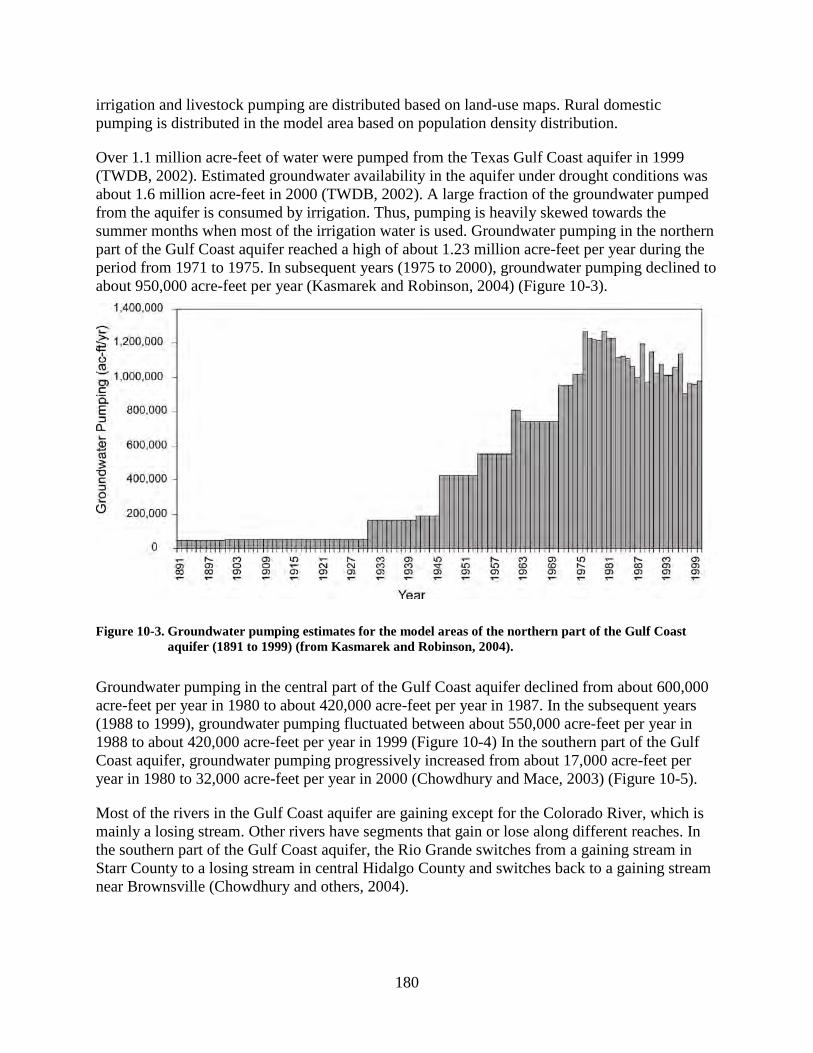
180

irrigation and livestock pumping are distributed based on land-use maps. Rural domestic pumping is distributed in the model area based on population density distribution.

Over 1.1 million acre-feet of water were pumped from the Texas Gulf Coast aquifer in 1999 (TWDB, 2002). Estimated groundwater availability in the aquifer under drought conditions was about 1.6 million acre-feet in 2000 (TWDB, 2002). A large fraction of the groundwater pumped from the aquifer is consumed by irrigation. Thus, pumping is heavily skewed towards the summer months when most of the irrigation water is used. Groundwater pumping in the northern part of the Gulf Coast aquifer reached a high of about 1.23 million acre-feet per year during the period from 1971 to 1975. In subsequent years (1975 to 2000), groundwater pumping declined to about 950,000 acre-feet per year (Kasmarek and Robinson, 2004) (Figure 10-3).

Figure 10-3. Groundwater pumping estimates for the model areas of the northern part of the Gulf Coast aquifer (1891 to 1999) (from Kasmarek and Robinson, 2004).

Groundwater pumping in the central part of the Gulf Coast aquifer declined from about 600,000 acre-feet per year in 1980 to about 420,000 acre-feet per year in 1987. In the subsequent years (1988 to 1999), groundwater pumping fluctuated between about 550,000 acre-feet per year in 1988 to about 420,000 acre-feet per year in 1999 (Figure 10-4) In the southern part of the Gulf Coast aquifer, groundwater pumping progressively increased from about 17,000 acre-feet per year in 1980 to 32,000 acre-feet per year in 2000 (Chowdhury and Mace, 2003) (Figure 10-5).

Most of the rivers in the Gulf Coast aquifer are gaining except for the Colorado River, which is mainly a losing stream. Other rivers have segments that gain or lose along different reaches. In the southern part of the Gulf Coast aquifer, the Rio Grande switches from a gaining stream in Starr County to a losing stream in central Hidalgo County and switches back to a gaining stream near Brownsville (Chowdhury and others, 2004).

181

Figure 10-4. Groundwater pumping estimates for the model areas of the central part of the Gulf Coast aquifer (1980 to 1999) (from Chowdhury and others, 2004).

Figure 10-5. Groundwater pumping estimates for the model areas of the southern part of the Gulf Coast aquifer (1980 to 1999) (from Chowdhury and Mace, 2003).

Conceptual Model

A conceptual model is our best understanding of the natural groundwater flow system. It describes how recharge, discharge, groundwater-surface water interactions, and cross-formational flow take place through the aquifers and the confining units of a flow system (Figure 10-6). When rain falls on the outcrop areas, much of it runs off to the rivers, a portion of it is lost through evaporation and transpiration, and less than about one percent reaches the saturated groundwater zone of the Gulf Coast aquifer. A portion of the water that reaches the saturated

182

Figure 10-6. A conceptual model of the Gulf Coast aquifer flow system, showing (a) groundwater flow components overlain on a cross-section through the middle of Jim Hogg, Brooks, and Kenedy counties; and (b) a numerical translation of the conceptual model (from Chowdhury and Mace, 2003).

groundwater zone flows laterally over small distances and discharges locally to streams. A small portion of the flow reaches the intermediate flow system at depth and a much smaller amount joins the deeper regional flow system, traveling considerable distances from the outcrop areas towards the Gulf of Mexico. As the flow reaches the saltwater-fresh water boundary near the coast, density differences between the fresh water and the salt water cause the regional groundwater flow to shift direction and move vertically upward toward coastal areas at lower elevations.

183

In general, groundwater flows from areas of higher topography towards lower topography. In this case, groundwater flows from the west towards the Gulf of Mexico in the east. However, considerable groundwater pumping in parts of the model area has greatly changed groundwater flow directions. For example, decades of extensive groundwater pumping in Harris-Galveston, Wharton, Victoria, and Kleberg counties has altered the natural flow system (Chowdhury and others, this volume). In these areas, a decline in the potentiometric (or water-level) surface and an increase in the hydraulic gradient are inducing greater flow into the deeper parts of the aquifer than would have otherwise occurred under natural conditions. The increase in the hydraulic gradient due to groundwater pumping also allows more interaction between the aquifers and their confining units.

Model Boundaries and Grid Design

The boundaries for the GAMs of the Gulf Coast aquifer are defined by (1) the limits of the outcrop in the west, (2) the Gulf of Mexico in the east or downdip limit of the freshwater (location where the total dissolved solids concentration reaches 10,000 milligrams per liter), (3) hydrologic divides along major rivers, and (4) groundwater divides away from major pumping centers. The model area for the northern part of the Gulf Coast aquifer extends from across the Louisiana border at the Sabine River to the Lavaca River in the south. The model area for the central part of the Gulf Coast aquifer extends along a groundwater divide through Colorado-Fort Bend-Brazoria counties to the north to a groundwater divide through Jim Hogg, Brooks, and Kenedy counties in the south. The model area for the southern part of the Gulf Coast aquifer extends from a groundwater divide through Jim Hogg, Brooks, and Kenedy counties to the north to the Rio Grande along the Texas-Mexico border in the south (Figure 10-2).

Modelers designed the models such that they can reproduce the groundwater flow system. We used MODFLOW-96 (Harbaugh and McDonald, 1996) to model groundwater flow in the Gulf Coast aquifer. All the cells have a uniform area of one square mile. TWDB staff chose this cell size to be small enough to reflect the density of input data and the desired output detail and large enough for the model to be manageable. Model layer 1 represents the Chicot aquifer; model layer 2 represents the Evangeline aquifer; model layer 3 represents the Burkeville Confining System; and model layer 4 represents the Jasper aquifer.

Model cells were made inactive when they fell outside the model area or when they were thin, because they were found to cause convergence problems during calibration. For the model of the northern part of the Gulf Coast aquifer, each model layer consisted of 137 rows and 245 columns for a total of 134,260 cells and 61,082 active cells. For the model of the central part of the Gulf Coast aquifer, each model layer consisted of 177 rows and 269 columns for a total of 190,452 cells and 56,736 active cells. For the model of the southern part of the Gulf Coast, each model layer consisted of 125 rows and 135 columns for a total of 67,500 cells and 27,000 active cells.

Modeling Approach

The modeling approach included: (1) calibrating a steady-state model to reproduce pre-development conditions and (2) calibrating a transient model to reproduce seasonal fluctuations

184

in water levels and flows in streams. Modelers first calibrated the steady-state model to determine stable boundary conditions and to simulate static water levels under pre-pumping or near equilibrium conditions. This time period ranges from 1890 to the 1940s for the northern part of the Gulf Coast aquifer, 1910 to 1940 for the central part of the Gulf Coast aquifer, and 1930 to 1980 for the southern part of the Gulf Coast aquifer. Modelers calibrated the steady-state models separately to reproduce water levels during these time periods.

The approach for calibrating the model was to reproduce water levels under steady-state conditions and reproduce seasonal water-level changes under transient conditions. Modelers focused their calibration on the Chicot and the Evangeline aquifers that are more widely used and contain numerous wells with water-level measurements.

Modelers quantified the calibration, or goodness of fit, between the simulated and measured water-level values using root mean square error (RMSE):

RMSE = 5.0

2)(/1

−∑ i

n

ism hhn

where n is the number of calibration points, hm is the measured hydraulic head at any point i, and hs is the simulated hydraulic head at the same point i.

Once the modelers completed calibrating the steady-state model, they used the model as a starting point for transient calibration. The TWDB requested the years 1981 to 2000 because this period contained the most accurate and recent water-use and water-level information.

There are considerable similarities in the modeling approaches used for the northern, central, and southern parts of the Gulf Coast aquifer. For example: (1) the conceptual model for all three models is the same in that groundwater recharges in the outcrop mainly from rainfall and discharges in the downdip areas near the coast; (2) the Chicot, Evangeline, and Jasper aquifers and Burkeville confining system form four model layers providing a uniform lateral extent and thickness to each model layer; (3) model cells have uniform one mile dimensions; and (4) models use the U.S. Geological Survey’s MODFLOW-96 code to simulate the groundwater flow system.

The main differences between the models lie in the MODFLOW packages used for simulation:

• MODFLOW’s Interbed Storage package was only used in the northern part of the Gulf Coast aquifer to simulate land-surface subsidence. There is a lack of documented information on land-surface subsidence in the central and southern parts of the aquifer.

• Recharge was simulated in the model for the northern part of the Gulf Coast aquifer using a General Head Boundary package; recharge was simulated in the central part of the Gulf Coast aquifer using MODFLOW’s Recharge package and applying a percent of spatially distributed rainfall according to soil characteristics; and recharge was calibrated in the southern part of the Gulf Coast aquifer using MODFLOW’s Recharge package and applying a percent of the spatially distributed rainfall.

185

• MODFLOW’s Evapotranspiration package was used in the models for the central and the southern parts of the Gulf Coast aquifer but not for the model in the northern part.

• MODFLOW’s General Head Boundary package, used in the northern part of the Gulf Coast aquifer for recharge simulations, was considered inclusive of the groundwater-surface water interaction; MODFLOW’s Streamflow Routing package was used in simulating groundwater-surface water interaction in the central part of the Gulf Coast aquifer; and MODFLOW’s River package was used in simulating groundwater-surface water interaction in the southern part of the Gulf Coast aquifer.

Northern Part of the Gulf Coast Aquifer

The MODFLOW’s General Head Boundary package was used to simulate recharge and discharge in the outcrops of the model area. The General Head Boundary package acts as a head-dependent flux boundary and flow depends on the head differences and vertical conductance between the water table and adjacent deeper zones. Application of the General Head Boundary as a constant-head source of water requires that the groundwater flow system does not show any long term trends in water-level change, which is probably valid for most of the model area except for in areas with excessive groundwater pumping (Kasmarek and Robinson, 2004).

Water-table altitudes were constructed using topography and subtracting a “trend surface” (a dataset of measured depths to water supplemented by interpolated depths to water). Flow between the streams and the aquifer system was not explicitly simulated, with the understanding that the General Head Boundary would account for the stream discharges to the level of accuracy at which such discharges are known (Kasmarek and Robinson, 2004). Initial transmissivity distributions were constructed with data from Wesselman (1967), Carr and others (1985), Baker (1986), and Kasmarek and Strom (2002). For outcrop areas, the initial vertical hydraulic conductivity was computed by dividing a constant vertical hydraulic conductivity by the cumulative clay thickness from land surface to the centerline of the outcropping hydrogeologic unit. For the subcrop areas, vertical hydraulic conductivity is computed internally by MODFLOW by multiplying a leakance by the grid-block area. Initial storativities of the sands are from Kasmarek and Strom (2002).

Land-surface subsidence and compaction of clays were simulated using MODFLOW’s Interbed-Storage package (Leake and Prudic, 1991). Initial values of elastic and inelastic clay storativity (specific storage multiplied by clay thickness) are taken from Kasmarek and Strom (2002), Gabrysch (1982), and Strom and others (2003a, 2003b, 2003c).

Central Part of the Gulf Coast Aquifer

To calibrate the model for the central part of the Gulf Coast aquifer, Chowdhury and others (2004) adjusted several parameters to observe which parameter had the greatest effect on simulated water levels. Through this initial sensitivity analysis, it was observed that the horizontal hydraulic conductivity of the Evangeline aquifer, recharge rate, and vertical leakance of the Chicot aquifer affected the model results. Calibration efforts revealed that the model calibration was non-unique, particularly with respect to the use of hydraulic conductivity and

186

leakance values. Application of increased recharge has no significant bearing on the water levels, because excess recharge discharges to the streams as baseflow.

An initial attempt was made to calibrate the model using distributed horizontal hydraulic conductivity. However, when Chowdhury and others (2004) assigned pumpage values in the model layers, they were unable to reproduce the water levels, particularly in the Evangeline and Jasper aquifers. The best-fit simulated water levels that they were able to produce use zoned horizontal hydraulic conductivity for the Evangeline aquifer. Chowdhury and others (2004) zoned the hydraulic conductivity into three smaller sub-zones and adjusted the values following the median of the distributed hydraulic conductivity. The vertical leakance values that they used are similar to other Gulf Coast models (Chowdhury and Mace, 2003; Kasmarek and Robinson, 2004).

Southern Part of the Gulf Coast Aquifer

To calibrate the model for the southern part of the Gulf Coast aquifer, Chowdhury and Mace (2003) assigned recharge as a percent of distributed mean annual rainfall from 1930 to 1980. They used MODFLOW’s Evapotranspiration package to simulate transpiration. They used vegetation coverage maps to locate vegetation types and density and observed that mesquite is the dominant vegetation in the model area, with the highest density occurring in central Kenedy and Jim Hogg counties. Chowdhury and Mace (2003) applied three sets of multipliers (0.001, 0.0012, and 0.0015) to the distributed rainfall grid to account for varying evapotranspiration rates due to differences in the density of mesquite. Using these multipliers, they obtained evapotranspiration rates that range from 4.14×10-6 to 9.11×10-6 feet per day.

Chowdhury and Mace (2003) used MODFLOW’s River package to simulate flow between the Chicot aquifer and the Rio Grande. Surface elevations for different segments of the river were estimated from topographic maps and the U.S. Geological Survey’s digital elevation model. River bottom elevation was set at ten feet below the river head elevation. River bed conductance was estimated using the formulation (K×L×W)/M where K is the hydraulic conductivity, L is the length of the river cell, W is the width of the river cell, and M is the sediment thickness. In the final calibration, Chowdhury and Mace (2003) used a river bed conductance of 100,000 feet per day, a sediment thickness of 1 foot, an average width of 10 feet, and a length of 5,280 feet. They assigned layer 1 as unconfined and layers 2, 3, and 4 as unconfined/confined. They allowed the model to calculate transmissivity and storativity based on saturated thickness. To simulate the movement of water out of the model and into the Gulf of Mexico, Chowdhury and Mace (2003) assigned constant heads across 10 miles of an area offshore, including the area of Matagorda Bay in layer 1. In the subsequent layers, they assigned a no-flow boundary in the east to allow upward vertical flow of water towards the discharge areas of the coastline.

To calibrate the model, Chowdhury and Mace (2003) adjusted the various parameters to observe which parameter had the most effect on simulated water levels. Through this initial sensitivity analysis, they observed that the recharge rate, evapotranspiration rate, and horizontal hydraulic conductivity of layers 1 and 2 had the greatest effect on the model results.

187

Calibration Results

Each of the modeling teams calibrated each of the GAMs for the Gulf Coast aquifer. We summarized below the steady state and transient calibration results of each effort.

Northern Part of the Gulf Coast Aquifer

The simulated water levels of the Chicot, Evangeline, and Jasper aquifers for the steady-state model show a general agreement with the measured water levels and conform to the conceptual model of a flow system where recharge enters in the outcrop and flows relatively short distances to discharge into streams or longer distances through deeper zones where it is discharged by upward leakage in topographically low areas near the coast (Kasmarek and Robinson, 2004). Transmissivities used for the calibration of the northern parts of the Gulf Coast aquifer are of the same orders of magnitude as those reported in previous studies (Wesselman, 1967; Jorgensen, 1975; Carr and others, 1985; Baker, 1986; Kasmarek and Strom, 2002; Ryder and Ardis, 2002). However, it was noted that higher transmissivity areas were coincident with larger drawdowns, which the authors considered an artifact of the model (Kasmarek and Robinson, 2004).

The simulated and measured cones of depression were nearly coincident. However, the simulations for 1977 and 2000 were unable to reproduce maximum depth of the cones of depression. In most cases, the simulated cones were about 100 feet smaller than the measured cones. The simulated cones of depression for 2000 match better to measured cones of depression than in 1977, which the authors attributed to an underestimation of groundwater pumping in 1977. Storativities used to simulate water level changes in the Chicot and Evangeline aquifers range from 1×10-4 to 0.2 and 4×10-5 to 0.2, respectively, reflecting aquifer conditions from water table to semi-confined to confined conditions (Kasmarek and Robinson, 2004).

The root mean square error for 1977 were 34 feet for the Chicot aquifer, 43 feet for the Evangeline aquifer, and 47 feet for the Jasper aquifer which corresponds to 7, 8, and 17 percent of the hydraulic head drop across the model area (Figure 10-7). The root mean square error for 2000 was about 31 feet for the Chicot aquifer, about 40 feet for the Evangeline aquifer, and about 34 feet for the Jasper aquifer (Figure 10-8).

Simulated land-surface subsidence closely matches measured subsidence in the Harris-Galveston-Fort Bend county area (Kasmarek and Robinson, 2004). Land-surface subsidence measuring up to ten feet has been measured in southeastern Harris County. Land surface has subsided by at least six feet over a larger area covering central to southeastern Harris County. Land surface has subsided by up to three feet in southeastern Jasper County (Kasmarek and Robinson, 2004).

188

Figure 10-7. Comparison of simulated to measured water levels for 1977 for the northern part of the Gulf Coast aquifer (from Kasmarek and Robinson, 2004).

Figure 10-8. Comparison of simulated to measured water levels for 2000 for the northern part of the Gulf Coast aquifer (from Kasmarek and Robinson, 2004).

189

Central Part of the Gulf Coast Aquifer

The calibrated model reasonably reproduces the spatial distribution of water levels in the Chicot, Evangeline, and Jasper aquifers and the Burkeville confining system for the steady-state conditions of 1910 to 1940. The root mean square error is about 21 feet (Figure 10-9). The root mean square error that we obtained from calibration is about five percent of the hydraulic head-drop across the model area and is well within the ten percent error usually sought for model calibration. The model accurately replicates the interpreted flow directions towards the Gulf of Mexico and the streams. The spatial distribution of water-level residuals (differences between simulated and measured water levels) appears unbiased towards any specific location in the model area.

Figure 10-9. Comparison of simulated to measured water levels for the steady-state calibration model for the southern part of the Gulf Coast aquifer (from Chowdhury and Mace, 2003).

Chowdhury and others (2004) compared simulated net gain-loss values produced by the model through some of the stream reaches with the measured streamflow values. The three stations that they examined included the Guadalupe River at Victoria, the San Bernard River near Boling, and the San Antonio River near Goliad. Historical stream-flow data from 1910 to 1940 were compared with steady-state simulated baseflow from the model. Their simulated values are somewhat lower than the baseflow. After they calibrated the steady-state model to water levels in the 1940s, they calibrated the model to transient water levels for 1980 to 1990.

An initial attempt to calibrate the transient model by adjusting specific storage and specific yield values within an acceptable range failed. When Chowdhury and others (2004) only adjusted storage values, they were unable to reproduce the drawdowns in Wharton, Victoria, and Kleberg counties. Therefore, they developed three sub-zones of hydraulic conductivity based on the median of the distributed hydraulic conductivity values. They assigned a vertical leakance of

190

1×10-9 feet per day over a small area near Kingsville to represent local beds and lenses of silt and fine sand.

Chowdhury and others (2004) reproduced seasonal water-level changes in the transient model using recharge based on climate changes. They used specific storage values of 0.000008, 0.000001, 0.00001, and 0.000008 for layers 1, 2, 3 and 4, respectively, and specific yield values of 0.05, 0.01, 0.005, and 0.05 for layers 1, 2, 3, and 4, respectively. The specific yield values of 0.01 to 0.005 that they used in the transient calibration may seem low for the unconfined portions of the aquifer. Typical specific yields of sedimentary materials in unconfined aquifers range from 0.14 to 0.38 (Freeze and Cherry, 1979). Chowdhury and others (2004) attempted to calibrate the model using higher specific yields, but they were unable to reproduce the required fluctuations to match the measured water levels. The lower specific yield that they used is more typical of semi-confined aquifers. They felt that the lower specific yields are appropriate for the Chicot, Evangeline, and the Jasper aquifers as they contain numerous interbedded silt and clay lenses.

The root mean squared error for calibration is 46 feet for 1989 and 36 feet for 1999 (Figure 10-10). Improvement in the root mean squared error for the 1999 transient calibration period was probably caused by (1) a much lower drawdown observed in 1999 than in 1989, which absorbed the effects of underestimated drawdown, and (2) fewer observations wells available with water-level measurements. The root mean squared error for the 1989 and 1999 calibration periods are 5.1 percent and 4.8 percent, respectively, of the hydraulic head drop across the model area.

Simulated distribution of the water-level surfaces for all model layers in 1989 and 1999 reasonably reproduces the measured values. Spatial distribution of the water-level residuals (measured water-levels at calibration well points subtracted from the simulated water-levels) appear unbiased across the model area (Chowdhury and others, 2004). In some areas, they were more successful in minimizing errors. For example, most of the central portion of the model has errors close to zero, while in parts of the southern portion of the model area near Kingsville where they have underestimated the drawdown, the errors are as large as 100 feet. When they compared the distribution of the residuals and their magnitudes for 1989 and 1999, we observe that there is an improvement in the water-level residuals because of a general recovery of the water levels in 1999.

The transient model does a reasonable job in matching the measured monthly and annual water-level trends throughout most of the model area, with the exception of a shift between simulated and measured water levels in some wells. In many wells, however, there is a good match between measured and simulated water levels throughout the model area (Figures 10-11 and 10-12).

Chowdhury and others (2004) compared simulated net gain-loss values on several stream reaches. Their simulated values were somewhat lower than the baseflow that would be expected from the streamflow hydrographs. However, the trend in the simulated net gain-loss follows the

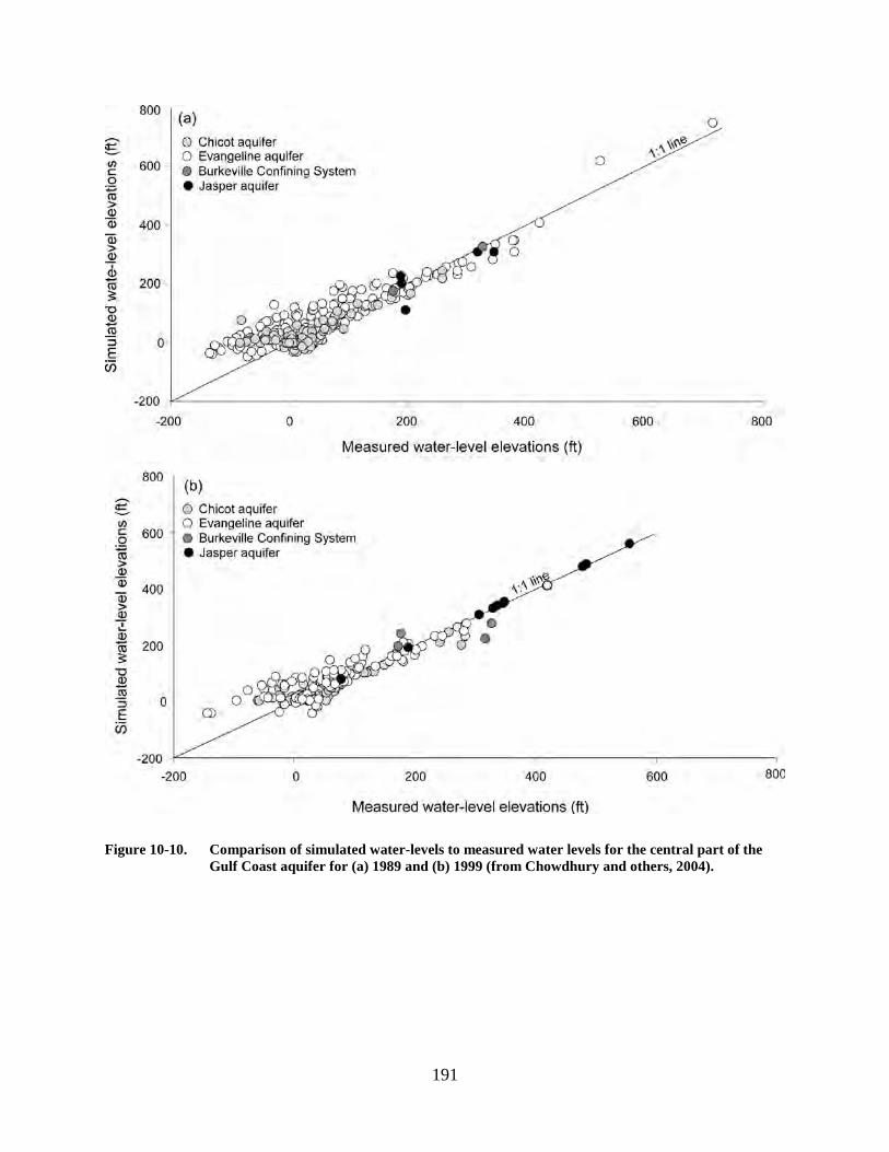
191

Figure 10-10. Comparison of simulated water-levels to measured water levels for the central part of the Gulf Coast aquifer for (a) 1989 and (b) 1999 (from Chowdhury and others, 2004).

192

(a) (b)

Figure 10-11. Comparison of simulated and measured water-level fluctuations in several wells for 1980 through 1999 for (a) well 7942702, (b) well 8011401, (c) well 8431201, and (d) well 8322801 for the GAM of the central part of the Gulf Coast aquifer (from Chowdhury and others, 2004).

(c)

(d)

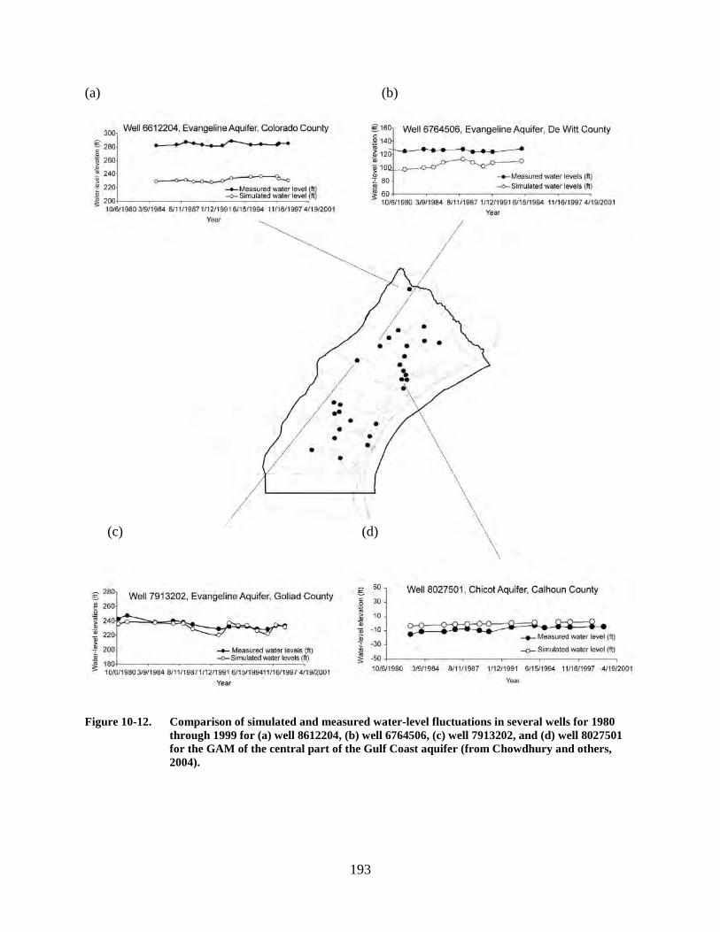
193

(a) (b)

Figure 10-12. Comparison of simulated and measured water-level fluctuations in several wells for 1980 through 1999 for (a) well 8612204, (b) well 6764506, (c) well 7913202, and (d) well 8027501 for the GAM of the central part of the Gulf Coast aquifer (from Chowdhury and others, 2004).

(c)

(d)

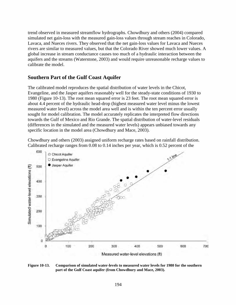
194

trend observed in measured streamflow hydrographs. Chowdhury and others (2004) compared simulated net gain-loss with the measured gain-loss values through stream reaches in Colorado, Lavaca, and Nueces rivers. They observed that the net gain-loss values for Lavaca and Nueces rivers are similar to measured values, but that the Colorado River showed much lower values. A global increase in stream conductance causes too much of a hydraulic interaction between the aquifers and the streams (Waterstone, 2003) and would require unreasonable recharge values to calibrate the model.

Southern Part of the Gulf Coast Aquifer

The calibrated model reproduces the spatial distribution of water levels in the Chicot, Evangeline, and the Jasper aquifers reasonably well for the steady-state conditions of 1930 to 1980 (Figure 10-13). The root mean squared error is 23 feet. The root mean squared error is about 4.4 percent of the hydraulic head-drop (highest measured water level minus the lowest measured water level) across the model area well and is within the ten percent error usually sought for model calibration. The model accurately replicates the interpreted flow directions towards the Gulf of Mexico and Rio Grande. The spatial distribution of water-level residuals (differences in the simulated and the measured water levels) appears unbiased towards any specific location in the model area (Chowdhury and Mace, 2003).

Chowdhury and others (2003) assigned uniform recharge rates based on rainfall distribution. Calibrated recharge ranges from 0.08 to 0.14 inches per year, which is 0.52 percent of the

Figure 10-13. Comparison of simulated water-levels to measured water levels for 1980 for the southern part of the Gulf Coast aquifer (from Chowdhury and Mace, 2003).

195

average annual rainfall for the years 1930 through 1980. A slightly lower recharge rate in the southern part of the Gulf Coast aquifer is more realistic, due to higher evaporation and lower rainfall than the rest of the Gulf Coast aquifer.

The maximum evapotranspiration rate was determined by trial and error during calibration. Groundwater extraction through evapotranspiration was assigned locally in areas where mesquite occurs. Given that the mean recharge is close to 0.5 percent of the mean annual rainfall, evapotranspiration could locally amount to as much as 19 to 29 percent of the recharge applied to calibrate the steady-state model.

The model has annual stress periods for 1980 to 2000 except for the drought years in each decade when monthly stress periods were assigned (1988, 1989, 1990 and 1994, 1995, and 1996). Chowdhury and others (2003) reproduced the water levels using recharge that reflects rainfall distribution for the time period and corresponding groundwater pumpage during that period. They reproduced the seasonal changes in the water levels by calibrating the specific storage and the specific yield values. They were able to best reproduce water-level changes using specific storage values of 0.000001, 0.000001, 0.00001, and 0.00001 for layers 1, 2, 3 and 4, respectively, and specific yield values of 0.001, 0.0005, 0.0001, and 0.001 for layers 1, 2, 3, and 4, respectively. The root mean squared error is 17 feet for 1980-1990 and 18 feet for 1990-2000 (Figures 10-14 and 10-15). The slight improvement in the root mean squared error for the transient calibration could simply be due to considering fewer wells than in the steady-state calibration.

The transient model does a reasonably good job of matching the measured monthly and annual water-level trends throughout most of the model area, with the exception of a shift between simulated and measured water levels (Figure 10-16). This shift in water levels has been carried over to the transient model from the steady-state model. In some wells, the shift was more pronounced than in others. This discrepancy is probably due to local-scale heterogeneity in the aquifer materials that we were unable to capture at the scale of the regional model as we averaged the aquifer properties within a model cell. Chowdhury and others (2003) also observed that, in some wells, simulated water levels for 1991 and 1992 were underestimated when there was considerable pumping. It is possible that the measured water levels for these years were taken during the winter months when the water level was high or that the wells had screen intervals in more than one aquifer. It is also possible that the shift in water levels could be caused by the calibration values that should coincide with the nodes of the model cells but in most cases they do not.

The specific yield values of 0.001 to 0.0005 that Chowdhury and others (2003) used in the transient calibration may appear low for the unconfined portions of the aquifer. Typical specific yields of sedimentary materials in unconfined aquifers range from 0.14 to 0.38 (Freeze and Cherry, 1979). They attempted to calibrate the model using higher specific yields but were unable to reproduce the required fluctuations to match the measured water levels. The lower specific yield that they used is more typical of semi-confined aquifers. They felt that the lower specific yields were appropriate for the Chicot, Evangeline, and the Jasper aquifers as the aquifers contain numerous clay beds and silt and clay lenses within the sands.

196

Figure 10-14. Comparison of simulated to measured water levels for 1990 for the southern part of the Gulf Coast aquifer (from Chowdhury and Mace, 2003).

Figure 10-15. Comparison of simulated to measured water levels for 2000 for the southern part of the Gulf Coast aquifer (from Chowdhury and Mace, 2003).

197

Figure 10-16. Comparison of simulated and measured water-level fluctuations in several wells for 1980 through 1999 for (a) well 8860701, (b) well 8756701, and (c) well 8763601 for the GAM of the southern part of the Gulf Coast aquifer (from Chowdhury and Mace, 2003).

198

Water Budget

A useful result of groundwater modeling is the ability to account for water budget on various components of flow in the aquifer. Water budgets provide information on where the water is coming from and where it is going. We summarize the results of the water budgets for each of the modeling projects below.

Northern Part of the Gulf Coast Aquifer

Simulation results indicate that total recharge through the outcrop areas in the steady-state was about 220,000 acre-feet per year (0.17 inches per year). Recharge mainly occurs through the outcrop of the Chicot aquifer (about 140,000 acre-feet per year); smaller quantities recharge through the Evangeline (about 49,000 acre-feet per year) and the Jasper aquifers (about 33,000 acre-feet per year); and negligible quantities recharge through the Burkeville Confining System (Kasmarek and Robinson, 2004). There are considerable differences between the pre-development and post-development recharge. Post-development recharge more than doubles to about 550,000 acre-feet per year in 1977 and 700,000 acre-feet per year in 2000 (Kasmarek and Robinson, 2004). Similarly, post-development discharge decreases from about 220,000 acre-feet per year to about 120,000 acre-feet per year in 1977 and to about 120,000 acre-feet per year in 2000. Therefore, much of the rejected recharge under pre-development condition is captured by the groundwater flow system to sustain groundwater pumping. It is notable that most of the recharge naturally discharges in the respective outcrops with only small fractions joining deeper, downdip parts of the aquifer.

Central Part of the Gulf Coast Aquifer

Chowdhury and others (2004) estimated the total volume of water that enters or leaves the system using the calibrated steady-state model. They found that about 540,000 acre-feet of water flows annually through the aquifer system. Of this total flow, 33 percent sources from rainfall that directly falls on the land surface in the outcrop areas of the model and 65 percent seeps into the aquifers from the numerous streams that cross the model area. When recharge values from rainfall alone are considered, they observed that about 66 percent of the recharge from rainfall infiltrates through the outcrops of the Chicot aquifer; about 21 percent infiltrates through the outcrops of the Evangeline aquifer; about 5 percent infiltrates through the outcrops of the Burkeville confining system; and about 8 percent through the outcrops of the Jasper aquifer.

Cross-formational flow between the different aquifers and the confining units are (1) about 20,000 acre-feet per year from the Evangeline aquifer to the overlying Chicot aquifer, (2) about 6,000 acre-feet per year from the Burkeville confining system to the overlying Evangeline aquifer, and (3) about 1,400 acre-feet per year from the Jasper aquifer to the Burkeville confining system.

Of the total annual flow of about 540,000 acre-feet, about 81 percent discharges into the streams and about 19 percent discharges into the Gulf of Mexico. Net loss of water from the aquifers

199

(baseflow discharge minus water inflow from the river) is about 46,500 acre-feet per year through the Chicot outcrop, about 24,000 acre-feet per year through the Evangeline outcrop, about 5,500 acre-feet per year through the Burkeville Confining System, and about 13,000 acre-feet per year through the Jasper outcrop. Both the reservoirs/lakes and the drains used to simulate the wetlands near the coast have only small volumes of water flowing through them.

The estimated water budget for the 1989 and 1999 calibration years are presented in Chowdhury and others (2004). They observed that stream discharge in 1989 is much lower than the pre-development model. The reduction in stream discharge in the transient model could presumably be attributed to groundwater pumping. Groundwater pumping is likely to capture groundwater flow that would have otherwise discharged naturally, causing reduced flow into and out of the streams. Discharge to the Gulf of Mexico is reduced in 1989 compared to the pre-development model. This observation is consistent with the findings from other recently developed models on the Gulf Coast aquifer system (Dutton and Richter, 1990; Ryder and Ardis, 2002; Kasmarek and Robinson, 2004).

Total recharge was considerably higher in 1989 than in the pre-development model probably due to capture of natural discharge (Chowdhury and others, 2004). Under natural conditions, groundwater recharge is balanced by discharge (Theis, 1940; Domenico and Schwartz, 1998). However, with continued decline in water level, a dynamic equilibrium is achieved either by increasing recharge and/or decreasing natural discharge. Recharge decreases again in 1999, coincident with the recovery of the water levels in the aquifer. Recovery of the water levels in 1999 occurs despite the fact that groundwater pumping in 1999 is at the same level as in 1989. Pumping in 1989 and 1999 are, however, considerably lower (by about 33 percent) compared to pumping of the early 1980s. This is probably why there is more recovery of the water levels in 1999. With the recovery of water levels in 1999, there is also a sharp decline in the amount of water movement out of storage into the flow system. This recovery in the water levels also results in an increase in stream discharge.

Southern Part of the Gulf Coast Aquifer

Chowdhury and Mace (2003) estimated the total volume of water that enters or leaves the system using the calibrated steady-state model. They found that about 87,000 acre-feet per year of water flows through the aquifer system. Of this total flow, 47 percent comes from rainfall that directly falls on the land surface in the outcrop areas of the model and 53 percent seeps into the aquifers from the Rio Grande. Nearly 62 percent of the total recharge from rainfall percolates through the Chicot outcrop; 32 percent percolates through the Evangeline outcrop; and the remainder (6 percent) percolates through the thin sliver of the Jasper outcrop. Of the total flow of about 87,000 acre-feet per year, 3 percent is lost through evapotranspiration, 15 percent discharges through pumping that existed during the 1980s, 32 percent flows into the Rio Grande and Arroyo Colorado, and 50 percent discharges to the Matagorda Bay and Gulf of Mexico. The amount of groundwater lost through evapotranspiration may appear low at the regional scale, but evapotranspiration may locally comprise up to 30 percent of recharge under steady-state conditions.

200

Conclusions

The Gulf Coast aquifer of Texas has had a number of models developed to better understand its flow characteristics and to provide management tools. The most recent models have been developed under the GAM program. Conclusions resulting from these modeling efforts are described below.

Northern Part of the Gulf Coast Aquifer

The calibrated model shows general agreement between simulated and measured water levels. The model reproduces the cones of depression in areas with excessive groundwater pumping. However, the model was unable to reproduce maximum depths of the cones of depression in some drawdown areas. The root mean squared errors that measure differences between simulated and measured water levels for 1977 are 34 feet for the Chicot aquifer, 43 feet for the Evangeline aquifer, and 47 feet for the Jasper aquifer. The root mean squared error for 2000 was 31 feet for the Chicot aquifer, 40 feet for the Evangeline aquifer, and 34 feet for the Jasper aquifer. Simulated hydrographs recording water level changes through the calibration period matches closely to measured hydrographs. Simulation results indicate that total recharge through the outcrop areas in the steady-state was about 220,000 acre-feet per year (0.17 inches per year). There are considerable differences between the pre-development and post-development recharge. Post-development recharge more than doubles to 550,000 acre-feet per year in 1977 and 700,000 acre-feet per year in 2000. Post-development discharge similarly decreases from about 220,000 acre-feet per year to about 120,000 acre-feet per year in 1977, and about 120,000 acre-feet per year in 2000. Therefore, much of the rejected recharge under pre-development conditions is captured by the groundwater flow system to sustain groundwater pumping. Most of the recharge naturally discharges in the respective outcrops, with only small fractions joining deeper, downdip parts of the aquifer. Simulated land-surface subsidence closely matches measured subsidence in the Harris-Galveston-Fort Bend county area.

Central Part of the Gulf Coast Aquifer

The calibrated model does a reasonable job of matching spatial distributions of water levels and water-level changes in well hydrographs with our data. The model reproduces the drawdown cones observed in Wharton, Victoria, and Kleberg counties in 1989 and 1999. The root mean squared error for calibration is about 21 feet for the pre-development period, 46 feet for 1989, and 36 feet for 1999.

About 540,000 acre-ft of water flows annually through the central Gulf Coast aquifer system in the pre-development model. Of this flow, 33 percent comes from rainfall and 65 percent seeps into the aquifers from the streams. Of the total annual flow of about 540,000 acre-feet, about 81 percent discharges into the streams, and about 18 percent discharges through the general head boundary into the Gulf of Mexico. Net loss of water from the aquifers (baseflow discharge minus water inflow from the river) is about 46,500 acre-feet per year through the Chicot outcrop, about 24,000 acre-feet per year through the Evangeline outcrop, about 5,500 acre-feet per year through

201

the Burkeville Confining System outcrop, and about 13,000 acre-feet per year through the Jasper outcrop.

Southern Part of the Gulf Coast Aquifer

The calibrated model generally replicates the spatial distribution of the water levels, maintaining the interpreted groundwater flow direction towards Gulf of Mexico and Rio Grande. The root mean squared error of the calibrated steady-state model is 23 feet—about 4.4 percent of the hydraulic head drop across the model area. The modelers used about 0.52 percent of the average annual rainfall for 1930 to 1980 to calibrate the steady-state model. They found that about 87,000 acre-feet per year of water flows through the aquifer system. Of the total flow, 47 percent comes from rainfall and 53 percent seeps into the aquifers from the Rio Grande. Cross-formational flow is a significant component of the total flow, with deeper groundwater from the Evangeline aquifer reaching upwards into the down-dip areas of the Chicot aquifer.

Acknowledgments

The U.S. Geological Survey developed the model for the northern part of the Gulf Coast aquifer with financial support from the Texas Water Development Board and the Harris-Galveston Subsidence District. Mr. Mark Kasmarek of the U.S. Geological Survey graciously provided figures and information for the northern part of the Gulf Coast aquifer.

References

Anderson, M. P., and Woessner, W. W., 1992, Applied groundwater modeling—Simulation of flow and advective transport: Academic Press, San Diego, 381 p.

Baker, Jr., E. T., and Wall, J. R., 1976, Summary appraisals of the nation’s groundwater resources—Texas Gulf region: U.S. Geological Survey Open-File Report, 61 p.

Baker, Jr., E. T., 1979, Stratigraphic and hydrogeologic framework of part of the coastal plain of Texas: Texas Department of Water Resources, Report 236, 43 p.

Baker, Jr., E. T., 1986, Hydrogeology of the Jasper aquifer in the southeast coastal plain: Texas Water Development Board Report 295, 64 p.

Carr, J. E., Sandeen, W. M., and McLane, I. R., 1985, Digital models for simulation of groundwater hydrology of the Chicot and Evangeline aquifers along the Gulf Coast of Texas: Texas Department of Water Resources Report 289, 101 p.

Chowdhury, A. H., and Mace, R. E., 2003, A groundwater availability model of the Gulf Coast aquifer in the Lower Rio Grande Valley, Texas—Numerical simulations through 2050: Texas Water Development Board Report, 171 p.

Chowdhury, A. H., Wade, S., Mace, R. E., and Ridgeway, C., 2004, Groundwater availability model for the central part of the Gulf Coast aquifer—Numerical simulations through 1999: Texas Water Development Board Report, 163 p.

202

Chowdhury, A. H., Bogichi, R., and Hopkins, J., this volume, Hydrochemistry, salinity distribution, and trace constituents—Implications for salinity sources, geochemical evolution, and flow system characterization, Texas Gulf Coast aquifer: Texas Water Development Board Report 365, p. 81–128.

Domenico, P. A. and Schwartz, F. W., 1998, Physical and chemical hydrogeology, New York, Wiley, 506 p.

Dutton, A. R., and Richter, B. C., 1990, Regional hydrogeology of the gulf coast aquifer in Matagorda and Wharton counties, Texas—Development of a numerical flow model to estimate the impact of water management strategies: Report prepared for the Lower Colorado River Authority under contract (88-89) 0910, Bureau of Economic Geology, The University of Texas at Austin, 118 p.

Freeze, R. A., and Cherry, J. A., 1979, Groundwater: Prentice Hall, Englewood Cliffs, New Jersey, 604 p.

Gabrysch, R. K., 1982, Groundwater withdrawals and land-surface subsidence in the Houston-Galveston region, Texas, 1906-80: U.S. Geological Survey Open-File Report 82-571, 58 p.

Gabrysch, R. K., 1984, Case history no. 9.12. The Houston-Galveston region, Texas, USA. in Poland, J. F., editor, Guidebook to studies of land subsidence due to groundwater withdrawal: UNESCO Studies and Reports in Hydrology 20, p. 253–262.

Groschen, G. E., 1985, Simulated effects of projected pumping on the availability of freshwater in the Evangeline aquifer in an area southwest of Corpus Christi, Texas: U.S. Geological Survey Water Resources Investigation Report 85-4182, 103 p.

Harbaugh, A. W., and McDonald, M. G., 1996, User’s documentation for MODFLOW-96, an update to the U.S. Geological Survey modular finite-difference ground-water flow model: U.S. Geological Survey Open-File Report 96-485, 56 p.

Harden and Associates, 2002, Availability of brackish groundwater from the Rio Grande alluvium, Cameron County, Texas: consultant report for the Southmost Regional Water Authority, 23 p.

Hay, R., 1999, A numerical groundwater flow model of the Gulf Coast aquifer along the South Texas Gulf Coast: M. S. Thesis, Texas A&M University—Corpus Christi, 47 p.

Jorgensen, D. G., 1975, Analog model studies of groundwater hydrology in the Houston district, Texas: Texas Water Development Board Report 190, 84 p.

Kasmarek, M. C., and Strom, E. W., 2002, Hydrogeology and simulation of ground-water flow and land surface subsidence in the Chicot and Evangeline aquifers, Houston area, Texas: U.S. Geological Survey, Water Resources Investigation Report 02-4022, 62 p.

Kasmarek, M. C., and Robinson, J. L., 2004, Hydrogeology and simulation of groundwater flow and land surface subsidence in the northern part of the Gulf Coast Aquifer System: U.S. Geological Survey Scientific Investigations Report, 2004-5102, 111 p.

Leake, S. A., and Prudic, D. E., 1991, Documentation of a computer program to simulate aquifer-system compaction using the modular finite-difference groundwater flow model:

203

U.S. Geological Survey Techniques of Water-Resources Investigations, Book 6, chapter A 2, 68 p.

Mace, R. E., 2001, Regional groundwater flow modeling in Texas: Texas Water Development Board (http://www.twdb.state.tx.us/gam/GAM_documents/texas_modeling.pdf).

Mace, R. E., Ridgeway, C., and Sharp, J., 2004, Groundwater is no longer secret and occult—A historical and hydrological analysis of the East case: Texas Water Development Board Report 361, Conference Proceedings 100 Years of Rule of Capture: From East to Groundwater Management, 26 p.

McCoy, T. W., 1990, Evaluation of groundwater resources in the Lower Rio Grande Valley, Texas: Texas Water Development Board Report 316, 47 p.

Meyer, W. R., and Carr, J. E., 1979, A digital model for simulation of groundwater hydrology in the Houston area, Texas: Texas Department of Water Resources LP-103, 27 p.

Noble, J. E., Bush, P. W., Kasmarek, M. C., and Barbie, D. L., 1996, Estimated depth to the water table and estimated rate of recharge in outcrops of the Chicot and Evangeline aquifers near Houston, Texas: U.S. Geological Survey Water Resources Investigations Report 96-4018, 19 p.

Ryder, P. D., 1988, Hydrogeology and pre-development flow in the Texas Gulf Coast aquifer systems: U.S. Geological Survey Water Resources Investigation report 87-4248, 109 p.

Ryder , P. D., and Ardis, A. F., 2002, Hydrology of the Texas Gulf Coast aquifer systems: U. S. Geological Survey Professional Paper 1416-E, 77 p.

Strom, E. W., Houston, N. A., and Garcia, C.A., 2003a, Selected hydrogeologic datasets for the Chicot aquifer, Texas: U.S. Geological Survey Open file Report 03-297, 1 CD-ROM.

Strom, E. W., Houston, N. A., and Garcia, C.A., 2003b, Selected hydrogeologic datasets for the Evangeline aquifer, Texas: U.S. Geological Survey Open file Report 03-298, 1 CD-ROM.

Strom, E. W., Houston, N. A., and Garcia, C. A., 2003c, Selected hydrologic data sets for the Jasper aquifer: U.S. Geological Survey Open File Report 03-299, 1 CD-ROM.

Theis, C. V., 1940, The source of water derived from wells—Essential factors controlling the response of an aquifer to development: Civil Engineering, American Society of Civil Engineers, p. 277-280.

TWDB, 2002, Water for Texas 2002: Texas Water Development Board Report, variously paginated.

Waterstone, 2003, Groundwater availability of the central Gulf Coast aquifer—Numerical simulations to 2050, Central Gulf Coast, Texas: Draft contract report submitted to Texas Water Development Board, Austin, Texas, variously paginated.

Wesselman, J. B., 1967, Groundwater resources of Jasper and Newton counties, Texas: Texas Water Development Board Report 59, 167 p.

Wood, L. A., and Gabrysch, R. K., 1965, Analog model study of groundwater in the Houston district, Texas: Texas Water Commission Bulletin 6503, 103 p.

204

This page intentionally blank.

205

Chapter 11

Optimization-Based Approaches for Groundwater Management

Venkatesh Uddameri1, Muthukumar Kuchanur1, and Naresh Balija1

Introduction Sustainable management of groundwater resources has gained increased attention in recent times, especially in the arid and semi-arid regions of Texas. The threat of large-scale unregulated pumping has spurred the creation of groundwater conservation districts in order to regulate the underlying aquifer resources in an efficient manner. Chapter 36 of the Texas Water Code and the more recent House Bill 1763 provide the legislative framework under which Groundwater Conservation Districts (GCDs) have to operate. In particular, GCDs have to develop a comprehensive management plan that addresses a variety of groundwater-related issues, including but not limited to: identifying efficient use of groundwater resources, addressing drought conditions, and characterizing surface water-groundwater interactions.

Obtaining reliable estimates for how much groundwater is available within a district is fundamental to its proper management. The available groundwater is a function of both aquifer hydrogeologic characteristics as well as the risk preferences of the decision makers’ involved. While a significant quantity of water is held in the subsurface, it is not practical or advisable to remove all of it over a short duration. The concept of safe yield suggests that the total withdrawals from the aquifer in a given time period should not exceed the recharge occurring over the same time period. While this approach is conceptually appealing, it is increasingly being considered inadequate as it does not account for the ecological demands on groundwater. In certain other areas, the anthropogenic demands on groundwater are large and exceed the amounts being recharged. In such instances, the depletion of groundwater is taken for granted, and the rate of depletion is managed to ensure that sufficient quantities of groundwater are available until alternative supplies are identified or water use is shifted to reduce the demand.

Groundwater management is a multi-stakeholder process wherein competing objectives and differing sets of values and perceptions have to be effectively reconciled. From a practical standpoint, consensus-based water management strategies and solutions are likely to succeed and lead to efficient use of groundwater (Mace and others, 2001). The challenge is to adequately capture the subjective preferences and concerns of the stakeholders and characterize them in terms of aquifer stimulus-response behavior.

1 Department of Environmental Engineering, Texas A&M University—Kingsville

206

The Texas Water Development Board (TWDB) has recently completed the development of groundwater availability models (GAMs) for major aquifers in Texas (for example, Chowdhury and others, 2004). These models utilize the conservation of mass and energy (Darcy’s law) to predict the response of the aquifer to various natural and anthropogenic stimuli such as recharge, pumping, and evapotranspiration. The response of the aquifer is characterized as the total hydraulic head (well water levels measured from a pre-specified datum). As stated previously, the available groundwater within a GCD is a function of both hydrogeology and public policy. GAMs only address the hydrogeologic part of the water availability equation. Hence, an additional instrument that combines GAM with the policy preferences of the stakeholders within a GCD is required to derive scientifically-credible, risk-informed, and consensus-based groundwater availability estimates.

The overall goal of this paper is to demonstrate how optimization tools developed in the field of operations research can be integrated with simulation models (GAMs) to objectively estimate groundwater availability by incorporating appropriate stakeholder preferences. The basic concepts required to set up the management model (optimization model) is presented next and is followed by illustrative case studies that combine optimization modeling with GAMs to develop decision support tools for estimating groundwater availability.

Optimization-Based Groundwater Management Models Optimization-based models for management are comprised of three parts: (1) the objectives that form the basis of management; (2) the constraints that limit the realization of the management objectives, and (3) the decision variables that control the management process. In optimization-based approaches, the decision variables are adjusted with the goal to maximize (or minimize) the objectives subject to meeting the constraints.

In the context of groundwater availability estimation, the objective functions could be maximizing the withdrawal of groundwater for economic gains and/or minimizing the withdrawal of groundwater to promote conservation. Multiple objectives such as maximizing pumping for economic gains and minimizing pumping for conservation or subsidence control can be simultaneously considered and such models are referred to as multiobjective optimization models. For groundwater availability estimation, constraints indicate the preferences and concerns of the stakeholders. Constraints could cover a gamut of issues, including: (1) ensuring that the pumping does not cause saltwater intrusion along the coast, (2) preventing subsidence from occurring, (3) protecting shallow wells from going dry, (4) making sure ecological requirements such as baseflows to streams and creeks are maintained, and (5) requiring that groundwater be equitably available to all stakeholders within the district. The decision variables could be point sources such as pumping at wells in different locations and areal sources/sinks like recharge rates indicating additional artificial recharge facilities or land use/land cover alterations that control evapotranspiration rates.

Both the objective and the constraints have to be the functions of the decision variable. If these functions are all linear, then the optimization model is called the linear programming model; otherwise, it is called a non-linear programming model. GAMs simulate the response of the aquifer to different imposed stresses. The state variable (total hydraulic head) at any location in

207

the model domain is a function of imposed stresses—pumping or alterations to recharge and evapotranspiration. Hence, if the constraints are specified in terms of the state variable, the relationship provided by the GAM could be used to establish the relationship between the constraints and the objective function.

For example, the management goal—“Large-scale pumping projects should not cause shallow domestic and livestock wells to go dry”—could be quantified as “the drawdown at a monitoring well due to any proposed large-scale pumping should not cause the water levels to drop more than 20 feet from their long-term average values.” The GAM can then be used to simulate the response of the aquifer when a new project is proposed and to establish a relationship between the pumping and the response at the monitoring well of interest. This relationship is then fed into the optimization model as a constraint to characterize the policy of GCD.

There are two approaches by which the responses from the simulation models such as GAMs can be incorporated into an optimization framework (Gorelick, 1983). In the embedded approach, the entire simulation model is included within the optimization framework. Alternatively, in the response function approach, the relationship between the stimulus (pumping at a well) and the response at a specified monitoring well is expressed as an algebraic relationship in the optimization model. GAM runs are carried out prior to the development of the management model to establish the necessary relationship between stimulus (pumping) and response (monitoring well heads). The embedded approach offers greater flexibility in terms of changing pumping and monitoring well locations during optimization exercises as the entire GAM is embedded within the optimization framework. However, development of such models requires considerable programming effort. In addition, the developed optimization models will be cumbersome and hard to interpret. As such, the response function approach is better suited for groundwater availability estimation and often employed in groundwater optimization studies (for example, Zhou and others, 2003).

The algebraic equation linking groundwater pumping to aquifer drawdown is noted to be linear for confined aquifers (Ahlfeld and Mulligan, 2000). As such, the total response at the monitoring well due to simultaneous pumping at different locations is equal to the sum of individual responses caused due to pumping at each well. Therefore, if the total number of new wells in a proposed project is N, a minimum of N+1 model runs will be required to obtain the necessary response at different monitoring wells for a given time-step. The stimulus-response relationship is nonlinear when the transmissivity of the aquifer changes with drawdown, as is the case in unconfined formations. However, if the pumping is not excessive, the assumption of linearity is noted to reasonably hold true in unconfined formations as well (Uddameri and Kuchanur, 2005). Suitable nonlinear formulations have been suggested in the literature (Maddock III, 1974) and can be employed when the assumption of linearity is not reasonable. While nonlinear optimization models are not difficult to conceptualize, certain computational complexities have to be dealt with in their implementation. Also, the number of GAM runs required to establish the nonlinear relationship can be substantial and adds to the modeling effort.

Groundwater practitioners and consultants often employ sensitivity studies to evaluate impacts of potential projects or altered situations on water levels in aquifers. At a mechanistic level, the optimization approach effectively automates this procedure and searches for all possible solutions (Ahlfeld and Mulligan, 2000). The optimization approach is also valuable from the

208

policy standpoint, as it requires relevant stakeholders and decision makers to identify and characterize goals, objectives, and constraints. Using optimization models in an interactive mode is helpful to foster sustainability debate and reach consensus-based groundwater management policies as envisioned by the state legislature.

The literature is replete with applications of combined simulation optimization approaches to groundwater management (for example, Willis and Finney, 1988; Finney and others, 1992; Emch and Yeh., 1998; Zhou and others, 2003; Uddameri and Kuchanur, 2005). Additional information about this approach can be obtained in Gorelick (1983) and Ahlfeld and Mulligan (2000). Case studies illustrating the application of optimization schemes for groundwater management in the Gulf Coast aquifer of Texas are discussed next.

Case Study I: Coupling Optimization with Steady-State Central Gulf Coast GAM The steady-state Central Gulf Coast aquifer Groundwater Availability Model (SS-CGC-GAM) described by Chowdhury and others (2004) was used to develop estimates for how much water is available for use in Refugio County, Texas. This county is predominantly rural and is experiencing very little growth. The water demands are estimated to be less than 3,000 acre-feet per year and projected to stay constant over the next several decades (TWDB, 2002). As such, the use of a steady-state model was deemed reasonable to obtain preliminary water availability estimates.

The groundwater in Refugio County, Texas, is mostly extracted from the unconfined Chicot and semi-confined Evangeline aquifers of the Gulf Coast aquifer. Hydrogeologic studies carried out by Mason (1963) indicate that the Evangeline Formation is more prolific and consists of considerable sand thicknesses. Hence, it is likely that future large-scale development of groundwater resources are likely to occur in this formation. Being a coastal county, concerns with regards to potential saltwater intrusion under large-scale pumping were expressed by many stakeholders and decision makers. In addition, many ranchers and farmers use windmills to extract groundwater for their livestock, especially in remote ranch locations where electricity is not readily available. Hence, regional-scale drawdowns incurred due to any proposed large-scale project were to be kept at a minimum to avoid negative economic externalities. Refugio County has three perennial rivers: the Aransas River in the south, the Mission River in the central part, and the San Antonio River in the north. Surface water-groundwater interactions near these rivers were deemed important to sustain low summer flows and for aquifer recharge during precipitation events. In addition, as the aquifer is shared by other adjoining counties, the impacts of any groundwater withdrawals in Refugio County on water levels in adjacent counties were to be assessed as well.

Based on the above considerations, a management scenario consisting of several pumping and monitoring wells was developed and is depicted in Figures 11-1 and 11-2. The monitoring wells labeled B are used to monitor water levels in adjoining counties. Similarly, the monitoring wells labeled R, C, and M were used to monitor heads near the rivers, within the county (to maintain regional groundwater gradients), and along the coast to monitor for saltwater intrusion, respectively. The objective then was to identify how much surplus groundwater is available in

209

Figure 11-1. Pumping and monitoring wells in the Chicot aquifer—Case Study I.

Figure 11-2. Pumping and monitoring wells in Evangeline aquifer—Case Study I.

210

the district, subject to constraints on saltwater intrusion, sustaining baseflows, and maintaining regional gradients. Mathematically, these constraints can be stated as (Uddameri and Kuchanur, 2005):

∑=

=

50

1:

i

iiQMax (1)

Subject to:

( ) 1012,1,, ,..., k andjMSLH kjMW ==∀∆−≥

(2)

(3) }6,5{};4,3{};2,1{},{2,10,,,, ==∀≥− kjandiHH kiCjiC

}8,7{};6,5{};4,3{};2,1{},{2,10,,,, ==∀≥− kjandiHH kiRjiR (4)

(5) 4,3,2,1,2,1)( ,,0,, ==∀−≥ kjHH kjBWkjBW φ

50,...,1

min,=∀≥ iQQ ii (6)

Equation (1) represents the objective of maximizing the amount of groundwater that can be safely pumped (Q) from the aquifer. The prevention of saltwater intrusion is captured in Equation (2) where hydraulic heads (H) monitored at ten locations along the coast (MW1, … , MW10) in both Chicot and Evangeline aquifers (j = 1, 2) are assumed to be below specified head (MSL - )∆ . Where MSL is the height of the mean sea level from a pre-specified datum (equal to zero when mean sea level is used as the datum) and ∆ is the magnitude of the depth below the sea level that can be tolerated. The value of ∆ was taken to be equal to zero in the baseline case.

The groundwater flow in the aquifers is from west to east. One important management objective was to ensure that any future groundwater development should not cause an alteration to this regional flow direction. Three well couplets each in Chicot and Evangeline formations (i = 1, 2) were selected at different locations, (C1, C2, C3, C4, C5, C6) as depicted in Figures 11-1 and 11-2, in order to enforce the constraint that the heads in the western section (at C1, C3, C5) were greater than the corresponding wells on the eastern side (at C2, C3, C5) as mathematically stated in Equation (3). Along the same lines, another management objective was to maintain groundwater flows towards streams to sustain baseflows during dry periods. A set of four well couplets each in Chicot and Evangeline aquifers (R1-R2, R3-R4, R5-R6, R7-R8) were used for this purpose and the management objective was mathematically stated using Equation (4).

The hydraulic heads in the adjoining counties could not fall below a pre-specified level (∆ ). This constraint is mathematically captured using Equation (5). Equation (6) implies that the flow rate (Q) in any management well should not be less than a pre-specified flow rate (Qmin) specific to that well. A nominal minimum flow rate of 100 acre-feet per year was assigned to ensure at least a certain degree of pumping at each well without rendering the linear programming result infeasible. The necessary response coefficients were generated by carrying out appropriate GAM runs and the management model was coded in an MS-EXCEL spreadsheet and solved using the WHATSBEST add-in (Lindo Systems Inc., 2005).

211

The results of the optimization model are summarized in Table 11-1. The illustrative results indicate that how much groundwater is available in Refugio County depends upon how much drawdown is deemed acceptable in adjoining districts, suggesting the need for cooperation and joint planning among neighboring districts.

Table 11-1. Estimated groundwater availability under various drawdown conditions at the Refugio County boundaries.

No. Saltwater intrusion

constraint (feet)

Boundary drawdown constraint

(feet)

Available groundwater

(acre-feet per year) 1 0 5 12409

2 0 25 30481

3 0 50 37247

4 0 100 39630

5 0 150 39650

Case Study II: Coupling Optimization with Transient Central Gulf Coast GAM The transient version of the Central Gulf Coast aquifer GAM (T-CGC-GAM) was coupled with optimization routines to evaluate the impacts of proposed large-scale pumping projects along the western sections of the Refugio County. Two potential well fields, one in the southwestern section and the other in the northwestern section, were simulated by placing ten production wells in the Evangeline Formation. A suite of monitoring wells similar to the ones used in the previous study was also employed in this scenario evaluation. The locations of the monitoring and pumping wells are schematically depicted in Figure 11-3. The management model can be mathematically stated as follows:

∑ ∑= =2000 1

,:t i

tiQMax (7)

Subject to:

2009,.....,200010,.....,1,2,1)(,,, ===∀∆−≥ tandkjMSLH tkjMW (8)

{ } { }{ }{ } 2009,.....,20006,5;4,3;2,1,,2,10,,,,,, ===∀≥− tandkjiHH tkictjic (9)

{ } { }{ }{ }{ } 2009,.....,20008,7;6,5;4,3;2,1,,2,10,,,,,, ===∀≥− tandkjiHH tkirtjiR (10)

2009,.....,20004,3,2,1,2,1)( 2000,,,,,, ===∀−≥ tandkjHH kjBWtkjBW φ (11)

2009200010,...,1

min,totiwhereQQ ti

=∀=≥ (12)

= =2009 10t i

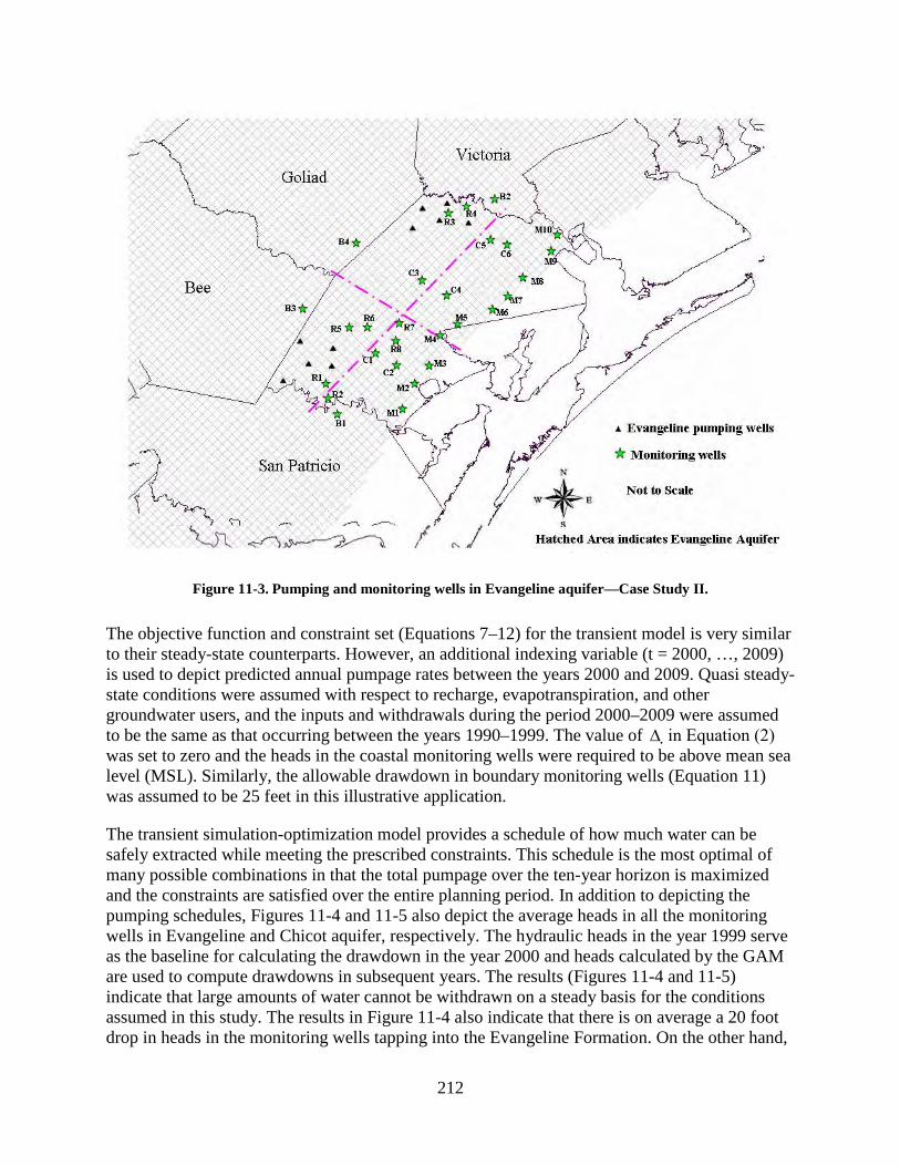
212

Figure 11-3. Pumping and monitoring wells in Evangeline aquifer—Case Study II.

The objective function and constraint set (Equations 7–12) for the transient model is very similar to their steady-state counterparts. However, an additional indexing variable (t = 2000, …, 2009) is used to depict predicted annual pumpage rates between the years 2000 and 2009. Quasi steady-state conditions were assumed with respect to recharge, evapotranspiration, and other groundwater users, and the inputs and withdrawals during the period 2000–2009 were assumed to be the same as that occurring between the years 1990–1999. The value of ∆ in Equation (2) was set to zero and the heads in the coastal monitoring wells were required to be above mean sea level (MSL). Similarly, the allowable drawdown in boundary monitoring wells (Equation 11) was assumed to be 25 feet in this illustrative application.

The transient simulation-optimization model provides a schedule of how much water can be safely extracted while meeting the prescribed constraints. This schedule is the most optimal of many possible combinations in that the total pumpage over the ten-year horizon is maximized and the constraints are satisfied over the entire planning period. In addition to depicting the pumping schedules, Figures 11-4 and 11-5 also depict the average heads in all the monitoring wells in Evangeline and Chicot aquifer, respectively. The hydraulic heads in the year 1999 serve as the baseline for calculating the drawdown in the year 2000 and heads calculated by the GAM are used to compute drawdowns in subsequent years. The results (Figures 11-4 and 11-5) indicate that large amounts of water cannot be withdrawn on a steady basis for the conditions assumed in this study. The results in Figure 11-4 also indicate that there is on average a 20 foot drop in heads in the monitoring wells tapping into the Evangeline Formation. On the other hand,

213

0

2000

4000

6000

8000

10000

12000

14000

1999 2000 2001 2002 2003 2004 2005 2006 2007 2008 2009

Year

Tot

al p

umpa

ge (a

cre-

feet

per

yea

r)

10.0

15.0

20.0

25.0

30.0

35.0

40.0

45.0

50.0

Hea

ds (f

eet)

Pumping ScheduleHeads in Evangeline

100Qmin (ac-ft/yr)

25.00Boundary Drawdown Constraint (ft)

0.00Saltwater Constraint (ft below MSL)

100Qmin (ac-ft/yr)

25.00Boundary Drawdown Constraint (ft)

0.00Saltwater Constraint (ft below MSL) φ

∆

Figure 11-4. Total pumpage versus average heads in the Evangeline aquifer for Case Study II.

0

2000

4000

6000

8000

10000

12000

14000

1999 2000 2001 2002 2003 2004 2005 2006 2007 2008 2009

Year

Tot

al p

umpa

ge (a

cre-

feet

per

yea

r)

0.05.010.015.020.025.030.035.040.045.050.055.060.065.070.075.0

Hea

ds (f

eet)

Pumping ScheduleHeads in Chicot

100Qmin (ac-ft/yr)

25.00Boundary Drawdown Constraint (ft)

0.00Saltwater Constraint (ft below MSL)

100Qmin (ac-ft/yr)

25.00Boundary Drawdown Constraint (ft)

0.00Saltwater Constraint (ft below MSL) φ

∆

Figure 11-5. Total pumpage versus average heads in the Chicot aquifer for Case Study II.

214

the hydraulic heads in the Chicot Formation are not affected by pumping in the Evangeline Formation, suggesting that the cross-formational flow in the TWDB GAM is not significant between the Chicot and Evangeline formations at the optimally derived pumping rates.

Sensitivity of the estimated water availability to the drawdown constraint at the county boundaries is schematically depicted in Figure 11-6. The results indicate that the specified drawdown at the boundary wells is significant if the acceptable drawdown is less than ten feet. Other constraints, notably the need to preserve regional groundwater gradients (Equation 9), affected the estimated water availability when the acceptable drawdown at the county boundaries was greater than ten feet.

0

5000

10000

15000

20000

25000

30000

2 5 10 25 50Boundary constraint (feet)

Tot

al p

umpa

ge o

ver

ten

year

s(a

cre-

feet

per

yea

r)

Figure 11-6. Sensitivity of the estimated water availability to the boundary drawdown constraint.

Summary and Conclusions Obtaining reliable estimates for groundwater availability is vital for efficient management of groundwater resources. The managed available groundwater in an aquifer is a function of both aquifer characteristics and public policy. GAMs developed by the Texas Water Development Board utilize conservation laws of physics to simulate the aquifer response characterized as hydraulic heads to various stresses (pumping, recharge, evapotranspiration, and other energy gradients). Optimization models can be established with specific management objectives (such as maximize groundwater extraction for economic gains) subject to environmental, ecological, and social constraints. The response from the GAMs can be used to characterize these constraints, and the combined simulation optimization models can be used to estimate groundwater availability and evaluate other policies.

The general simulation optimization approach has been discussed in this paper and two case studies demonstrating the utility of integrating GAMs with optimization schemes have been

215

illustrated. These real-world case studies demonstrate the utility of optimization schemes in groundwater management. The optimization approach effectively automates this procedure and searches for all possible solutions and as such is superior to conventional sensitivity analysis. The optimization approach is also valuable from the policy standpoint, as it requires relevant stakeholders and decision makers to identify and characterize goals, objectives, and constraints. Optimization models abstract the essential features of GAMs that are pertinent to the specific problems and therefore are more intuitive to understand. Application of these models in an interactive mode could help stakeholders understand the economic, environmental and ecological implications of proposed policies and help reach consensus-based groundwater management objectives as envisioned by the state legislature.

Acknowledgments The financial support from the National Science Foundation as well as from the Refugio Groundwater Conservation District is gratefully acknowledged.

References Ahlfeld, David P. and Mulligan, A. E., 2000, Optimal management of flow in groundwater

systems: San Diego, CA, Academic Press, 181 p.

Chowdhury, A. H., Wade, S., Mace, R. E., and Ridgeway, C., 2004, Groundwater availability model of the Central Gulf Coast Aquifer System—Numerical simulations through 1999: Texas Water Development Board draft report, 108 p.

Emch, P. G., and Yeh W. W.-G., 1998, Management model for conjunctive use of coastal and surface water and groundwater: Journal of Water Resources Planning and Management, v. 124, no. 3, p. 129–139.

Finney, B. A., Samsuhadi, S., and Willis, R., 1992, Quasi-three-dimensional optimization model of Jakarta basin: Journal of Water Resources Planning and management, v. 118, no. 1, p. 18-31.

Gorelick, S. M., 1983, A review of distributed parameter groundwater management modeling methods: Water Resources Research, v. 19, no. 2, p. 305–319.

Lindo Systems, Inc., NY , 2005, Online access: www.lindo.com.

Mace, R. E, Mullican, W. F., and Shao-Chih, 2001, Estimating groundwater availability in Texas, in Proceedings of the Texas Rural Water Association and Texas Water Conservation Association Water Law Seminar, 1st—Water allocation in Texas—The legal issues, Austin, Texas, January 25–26, 2001.

Maddock III, T., 1974, The operation of a stream-aquifer system under stochastic demands: Water Resources Research, v. 10, no. 1, p. 1–10.

Mason, C., 1963, Ground water resources of Refugio County, Texas: Texas Water Commission Bulletin 6312, Austin, Texas, 115 p.

Texas Water Development Board, 2002, Water for Texas—2002: TWDB, Austin, Texas, 156 p.

216

Uddameri, V., and Kuchanur, M., 2005, Simulation-optimization approach to assess groundwater availability in Refugio County, Texas: to be submitted to Environmental Geology.

Willis, R., and Finney, B. A., 1988, Planning model for control of salt water intrusion: Journal of Water Resources Planning and Management, v. 114, no. 3, p. 333–347.

Zhou X., Chen M., and Liang C., 2003, Optimal schemes of groundwater exploitation for prevention of seawater intrusion in the Leizhou peninsula in southern China: Environmental Geology, v. 43, no. 8, p. 978–985.

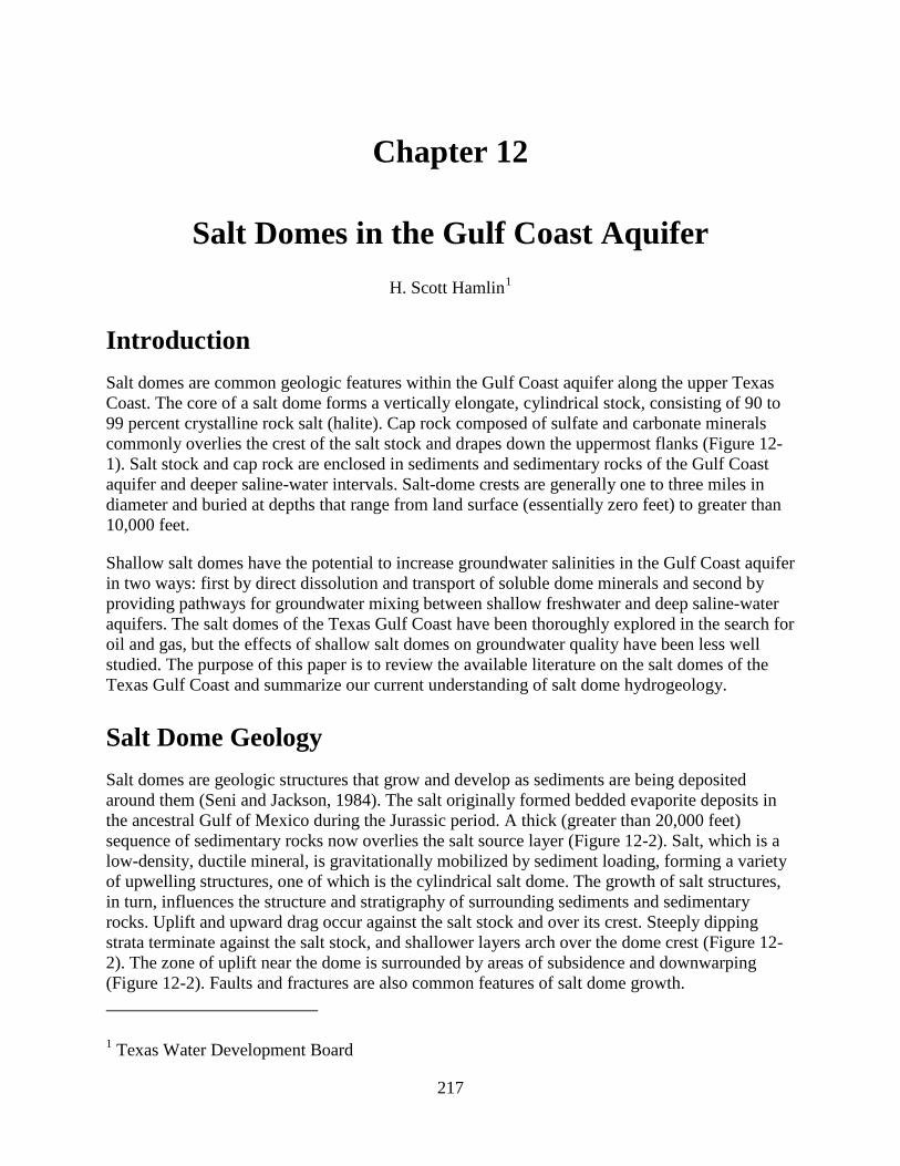
217

Chapter 12

Salt Domes in the Gulf Coast Aquifer H. Scott Hamlin1

Introduction Salt domes are common geologic features within the Gulf Coast aquifer along the upper Texas Coast. The core of a salt dome forms a vertically elongate, cylindrical stock, consisting of 90 to 99 percent crystalline rock salt (halite). Cap rock composed of sulfate and carbonate minerals commonly overlies the crest of the salt stock and drapes down the uppermost flanks (Figure 12-1). Salt stock and cap rock are enclosed in sediments and sedimentary rocks of the Gulf Coast aquifer and deeper saline-water intervals. Salt-dome crests are generally one to three miles in diameter and buried at depths that range from land surface (essentially zero feet) to greater than 10,000 feet.

Shallow salt domes have the potential to increase groundwater salinities in the Gulf Coast aquifer in two ways: first by direct dissolution and transport of soluble dome minerals and second by providing pathways for groundwater mixing between shallow freshwater and deep saline-water aquifers. The salt domes of the Texas Gulf Coast have been thoroughly explored in the search for oil and gas, but the effects of shallow salt domes on groundwater quality have been less well studied. The purpose of this paper is to review the available literature on the salt domes of the Texas Gulf Coast and summarize our current understanding of salt dome hydrogeology.

Salt Dome Geology Salt domes are geologic structures that grow and develop as sediments are being deposited around them (Seni and Jackson, 1984). The salt originally formed bedded evaporite deposits in the ancestral Gulf of Mexico during the Jurassic period. A thick (greater than 20,000 feet) sequence of sedimentary rocks now overlies the salt source layer (Figure 12-2). Salt, which is a low-density, ductile mineral, is gravitationally mobilized by sediment loading, forming a variety of upwelling structures, one of which is the cylindrical salt dome. The growth of salt structures, in turn, influences the structure and stratigraphy of surrounding sediments and sedimentary rocks. Uplift and upward drag occur against the salt stock and over its crest. Steeply dipping strata terminate against the salt stock, and shallower layers arch over the dome crest (Figure 12-2). The zone of uplift near the dome is surrounded by areas of subsidence and downwarping (Figure 12-2). Faults and fractures are also common features of salt dome growth. 1 Texas Water Development Board

218

Figure 12-1. Generalized cross section of a salt dome showing salt stock and cap rock mineralogical zones (modified from Halbouty, 1979).

Salt dome growth also influences the topography of the overlying land surface. Positive topographic relief is linked to uplift, whereas subsidence of the topographic surface is linked to dissolution of the dome crest (Seni and Mullican, 1986; Mullican, 1988). Of the shallow domes along the upper Texas Gulf Coast, 63 percent have positive topographic relief over their crests (Seni and others, 1984d). Warping of the depositional surface, either on the coastal plain or in the shallow marine environment, influences sedimentation patterns. Muddy sediments tend to be deposited over dome crests, and sandy sediments tend to be deposited in surrounding downwarped areas.

Salt dome cap rock is composed mainly of anhydrite, gypsum, and calcite arranged in heterogeneous layers (Figure 12-1). Cap rock formation results from salt dissolution. Anhydrite (calcium sulfate), the main impurity in the salt stock, forms a residual accumulation at the dome crest. Other geochemical processes convert the anhydrite to gypsum (hydrous calcium sulfate),

219

Figu

re 1

2-2.

Reg

iona

l dip

-ori

ente

d cr

oss s

ectio

n th

roug

h th

e G

ulf C

oast

Bas

in so

uthw

est o

f Hou

ston

in

ters

ectin

g a

num

ber

of sa

lt do

mes

(mod

ified

from

Ham

lin, 1

986)

. Lin

e of

sect

ion

show

n in

Fi

gure

12-

3.

220

calcite (calcium carbonate), and to a lesser extent, native sulfur and metallic sulfides (Bodenlos, 1970; Kyle and Price, 1986). Cap rock layering is irregular and varies greatly from dome to dome. Structural deformation and fracturing are common, as are cavernous voids. Gulf Coast cap rocks range in thickness from 0 to 2,000 feet. Cap rocks are direct evidence for dissolution of salt by groundwater.

Most of the salt domes along the Gulf Coast of Texas occur in the northeast (Figure 12-3). The base of fresh to slightly saline water (less than 3,000 mg/L of total dissolved solids [TDS]) in the Gulf Coast aquifer varies but is generally less than 3,000 feet (Baker, 1979); therefore, shallow salt domes whose crests are less than 3,000 feet deep are the ones that could affect fresh groundwater quality. There are 3 shallow salt domes in South Texas southwest of Corpus Christi and 35 along the upper coast (Figure 12-3). Because there is a gap in depth distribution between shallow and deep salt domes, the maximum depth of shallow domes is only 1,500 feet. The average depth is 565 feet. Average cap rock thickness is 481 feet (Figure 12-4).

Natural Resources Salt domes provide a variety of natural resources (Seni, 1986). Structural deformation and cap rock formation have created prolific petroleum reservoirs. Oil and gas are trapped in uplifted strata surrounding or overlying salt domes and in the cap rock itself. In addition to petroleum, salt from the salt stock and sulfur from the cap rock are the main commodities derived from Gulf Coast salt domes in Texas (Figure 12-5). Salt domes also provide space for storage and disposal (Seni and others, 1985). Solution-mined caverns in the salt stock have been created both for brine production and for storage of various petroleum products, most commonly liquid petroleum gas. The volume of some storage caverns exceeds ten million barrels. Crude oil for the Strategic Petroleum Reserve is stored in caverns at several Texas Gulf Coast salt domes. Cavernous zones in cap rocks have been used for brine disposal (Seni and others, 1984c), and the potential for disposal of chemical wastes in salt caverns has been evaluated (Seni and others, 1984a).

Resource development and production can create geologic and hydrologic instabilities around salt domes (Seni and others, 1985). Land-surface subsidence, sometimes involving catastrophic collapse and sinkhole formation, is common where large amounts of sulfur, salt, and/or petroleum have been extracted from the salt dome (Mullican, 1988). High-volume brine disposal elevates cap rock fluid pressures in shallow intervals laterally adjacent to freshwater sands, reversing pre-development hydraulic gradients and creating the potential for aquifer contamination (Hamlin and others, 1988). Petroleum storage caverns in the salt stock have failed and leaked product into surrounding freshwater sands (Seni and others, 1984b, 1985).

Hydrogeologic Units A salt dome in the Gulf Coast aquifer forms a complex system of hydrogeologic units. The salt stock is a cylindrical vertical aquiclude. The cap rock rests on the salt stock like an inverted cup. Cap rocks are essentially karstic aquifers whose hydrodynamic properties are controlled by fracturing and dissolution. Irregularly distributed networks of vuggy to cavernous porosity are

221

Figure 12-3. Map of shallow salt domes in the Gulf Coast aquifer in Texas. Also showing line of cross section in Figure 12-2 (compiled from Seni and others, 1984b-d, 1985).

222

Figure 12-4. Map of shallow salt domes in the Gulf Coast aquifer showing relative depths and cap rock thicknesses. The salt domes are shown schematically extending above a datum at 3,000 feet below sea level. Depth and thickness statistics also shown (Compiled from Beckman and Williamson, 1990, and Seni and others, 1984b-d, 1985).

223

Figure 12-5. Maps of shallow salt domes in the Gulf Coast aquifer showing natural resources. Petroleum resources (not shown) have been developed at most Gulf Coast salt domes (compiled from Seni and others, 1984b-d, 1985).

common in cap rock. Drillers name these networks “lost-circulation zones” because of the difficulty of establishing drilling-fluid circulation in wells penetrating cavernous intervals. These are also the intervals favored for brine disposal because they readily accept high injection rates. However, cap rock also includes areas composed of dense calcite and anhydrite, which have low hydraulic conductivity.

The salt stock and cap rock are encased in interbedded sandy aquifers and muddy aquitards. In these interbedded sand and mud layers, hydraulic conductivity in the horizontal direction is typically many times greater than it is in the vertical direction. However, the potential for high

224

vertical hydraulic conductivity exists within the zone of structural deformation around the salt dome. Gulf Coast salt domes contact freshwater sands in the Chicot, Evangeline, and Jasper aquifers, as well as saline-water sands in more deeply buried intervals (Figure 12-2).

Salt Domes and Groundwater Flow The arrangement and physical properties of aquifers and aquitards in the salt dome environment delineate possible pathways for groundwater flow, but additional evidence is needed to document actual groundwater flow. Fluid-pressure gradients must be known to establish hydraulic driving forces for flow, and groundwater chemical compositions must be known to trace groundwater sources and mixing. Ideally, all available geologic and hydrologic data should be assembled in a conceptual model of the system that can then be translated into a numerical model of three-dimensional, density dependant groundwater flow around the salt dome. This section reviews the available hydrodynamic and hydrochemical evidence for groundwater flow around salt domes along the Texas Gulf Coast.

Evidence from Hydraulic Heads

In the salt-dome environment, groundwater flow is driven not only by hydraulic-head gradients but also by density gradients. The density gradients arise from the high thermal conductivity of salt and from groundwater salinity variations due to dissolution of the salt itself (Evans and others, 1991). Few studies have reported head and density distributions in the vicinity of Texas coastal salt domes. Work done in East Texas, where salt domes penetrate the Carrizo-Wilcox aquifer, suggests that dome-related uplift creates local recharge areas over some salt-dome crests, but in general regional flow patterns are not affected by the presence of salt domes (Fogg and others, 1983). Studies in Louisiana, where salt domes penetrate the Gulf Coast aquifer, document upward groundwater flow around deeper dome flanks but downward flow at shallower levels (Evans and others, 1991), although the focus of the Louisiana studies was the interval below the base of freshwater.

At Barbers Hill salt dome, which penetrates Evangeline and Chicot freshwater sands in Chambers County, head measurements and pumping tests were conducted in the cap rock aquifer, which is saturated with dense brine (Hamlin and others, 1988). Barbers Hill salt dome has a history of intense development, including oil production, salt-cavern storage, and cap rock brine disposal. Water-level data are available from cap rock disposal wells. When the effects of density variations were normalized, a hydraulic gradient directed radially outward and upward from the cap rock was revealed. The present magnitude and direction of this hydraulic gradient is attributable both to lowering of fluid pressures in the Chicot and the Evangeline aquifers by long-term pumping in the Houston area and to elevation of fluid pressures in the cap rock by high-volume brine disposal.

Controlled brine injection tests at Barbers Hill salt dome indicated that the cap rock is a single integrated aquifer with leaky vertical and lateral boundaries. Because of the arched shape of the cap rock (Figure 12-1), the vertical boundary corresponds to vertical and lateral contacts with freshwater sands, and the lateral boundary is the lower edge down the dome flanks that is in contact with deeper saline-water sands. Within the cap rock, water levels stabilized in

225

observation wells during a long-term (29 days) brine injection test, showing that groundwater must be exiting the cap rock (Figure 12-6). During the brine injection test, however, water levels were not monitored in nearby Chicot and Evangeline water wells, so the exact destination of leaking cap rock brines was not documented.

Figure 12-6. Hydrograph of a long-term cap rock injection test at Barbers Hill salt dome showing brine-level changes in a cap rock observation well during controlled brine disposal in two other cap rock wells. Water levels in nearby Chicot and Evangeline wells are around 100 feet below sea level or similar to cap rock brine levels when no disposal is occurring (modified from Hamlin and others, 1988).

Evidence from Groundwater Chemistry

Hydrochemical patterns in groundwater near salt domes provide information about flow of dome-related fluids into surrounding freshwater aquifers. The most commonly available data for measuring groundwater salinities in the near-dome environment are geophysical logs from oil and gas wells, because an empirical relationship can be established between groundwater salinity and electrical conductivity (Jones and Buford, 1951) and because most salt domes have been densely drilled in the quest for oil. Using geophysical logs, anomalously high salinities in shallow sands were documented near salt domes in Chambers, Fort Bend, and Jefferson counties (Wesselman, 1971, 1972).

At Barbers Hill salt dome, Hamlin and others (1988) used closely spaced well logs to map individual sand bodies and groundwater salinities near the dome, revealing a complicated pattern of vertical and lateral salinity variation (Figure 12-7). In one Chicot sand, a plume of high-salinity groundwater extends away from the salt dome in the direction of regional groundwater flow (Figure 12-8). Similar saline plumes extending away from salt domes in the direction of groundwater flow have been documented in the Carrizo-Wilcox aquifer in East Texas (Fogg and others, 1983) and in Germany (Klinge and others, 2002).

Chemical and isotopic analyses of groundwater are less abundantly available than are geophysical logs but can be used to reveal both fluid sources and flow patterns. Banga and others

226

Figure 12-7. North-south cross section across Barbers Hill salt dome showing Chicot and Evangeline sands and groundwater salinities near and in contact with the cap rock. Groundwater salinities were interpreted from geophysical logs. Individual sand bodies were correlated and mapped using closely spaced geophysical and drillers logs. A map of salinity in the lower Chicot sand is shown in Figure 12-8 (modified from Hamlin and others, 1988).

(2002) used multi-element chemistry and isotopic tracers to document vertical flow patterns in deep sandstones (below freshwater) around South Liberty salt dome in Liberty County, showing that oil field brines near the salt dome are a mixture of shallow meteoric waters and deep formation waters. The presence of a meteoric component in deep brines indicates downward flow along the flanks of the salt dome. The implication of the South Liberty salt dome study is that shallow fresh groundwater flows across the top of the salt dome, dissolves salt, becomes increasingly dense, and then flows downward along the dome flanks driven by a density gradient.

227

Figure 12-8. Map of groundwater salinity in a lower Chicot sand at Barbers Hill salt dome. Salinities were measured in water wells and calculated from geophysical logs. Anomalously high salinities on the southwest side of the dome outline a plume of saline water extending away from the salt dome in the down-flow direction (modified from Hamlin and others, 1988).

Evidence from Numerical Modeling

Numerical modeling of groundwater flow systems around salt domes has proved challenging owing to the complications of extreme salinity and density variations and complex boundary conditions (Konikow and others, 1997). Fogg and others (1983) modeled groundwater flow in the Carrizo-Wilcox aquifer around a salt dome but without explicitly including the dome itself or salinity variations. Their model helped identify recharge and discharge areas and flow paths in freshwater aquifer sands relative to the position of the salt dome, so that the movement of potential dome-related contaminants might be predicted. Their model also showed the importance of sand-body distribution and interconnection as controls on flow near salt domes. Hamlin and others (1988) modeled the cap rock aquifer at Barbers Hill salt dome, using the results of controlled brine injections tests, but did not include the surrounding Chicot and Evangeline sands or salinity/density variations. Nevertheless, their model accurately reproduced water-level measurements and demonstrated that the cap rock boundaries are leaking. Models of groundwater flow around Gulf Coast salt domes in Louisiana, which explicitly include both the

228

salt dome and salinity/density variations, emphasize the importance of density-driven flow (Evans and others, 1991). The Louisiana models show that salt dissolved at the dome crest is carried down the dome flanks below the zone of freshwater.

Discussion The evidence for dissolution of salt dome minerals in shallow groundwater is conclusive. Shallow salt domes extend well into the zone of freshwater and are surrounded laterally and vertically by Gulf Coast aquifer sands. As salt dissolves at the dome crest, an insoluble residue accumulates, forming the cap rock. Within the cap rock itself, chemical reactions occur that require the presence of low-temperature, low-salinity groundwaters (Kyle and Price, 1986). Geophysical logs have been used to identify high-salinity plumes within otherwise freshwater sands near several Gulf Coast salt domes and to map actual sand/dome contacts (Figure 12-7). Indeed, dissolution of salt domes by groundwater has been documented, and the amount of salt removed has been quantified (Seni and Jackson, 1984; Bruno and Hanor, 2003).

Although salt actively goes into solution at the crests of shallow salt domes, most of the high-salinity groundwater thus formed flows downward driven by density gradients. Recent studies document downward flow along salt-dome flanks and the control of faults and sand distribution on flow paths (Banga and others, 2002; Bruno and Hanor, 2003). Although upward flow occurs in deep zones below the base of freshwater (Evans and others, 1991), upward movement and mixing of dense saline groundwater from deep zones into the low-density freshwater zones appears unlikely.

Development of both fresh groundwater and salt-dome resources has increased the potential for contamination of shallow aquifers. In pre-development steady-state groundwater flow systems, salt-dome related contamination remained localized by high freshwater heads in surrounding sands and the tendency for high-density brines to flow downward. The combination of lowered heads in the Gulf Coast aquifer and increased heads in cap rocks has created hydraulic gradients directed outward from the salt dome toward adjacent freshwater sands. Resource extraction and leakage of stored petroleum product have further perturbed the natural system. Most of the available evidence for salt-dome-related contamination of the Gulf Coast aquifer is at least 20 years old. More recent hydraulic and hydrochemical data, including data collected periodically through time, are needed for proper risk analysis and for a more comprehensive understanding of groundwater flow near salt domes.

Acknowledgments This review of salt dome hydrogeology is based primarily on research supported by the Texas Department of Water Resources and the Texas Water Commission during 1984 and 1985. Steven J. Seni, William F. Mullican, III, and I were the primary researchers. Since that time relatively little has been published on the effects of salt domes on Gulf Coast groundwater resources. Thanks to Steve and Bill for allowing me to mine their work for material for this paper, which I hope may generate renewed interest in the subject. Thanks also to Sarah Davidson for making the Gulf Coast aquifer conference and publication happen.

229

References Baker, E. T., Jr., 1979, Stratigraphic and hydrogeologic framework of part of the Coastal Plain of

Texas: Texas Department of Water Resources Report 236, 43 p.

Banga, T., Capuano, R. M., and van Nieuwenhuise, D. S., 2002, Fluid flow, stratigraphy and structure in the vicinity of the South Liberty salt dome, Texas: Gulf Coast Association of Geological Societies Transactions, v. 52, p. 25–36.

Beckman, J. D., and Williamson, A. K., 1990, Salt-dome locations in the Gulf Coastal Plain, south-central United States: U.S. Geological Survey Water-Resources Investigations Report 90-4060, 44 p.

Bodenlos, A. J., 1970, Cap-rock development and salt-stock movement, in Kupfer, D. H., editor, Geology and technology of Gulf Coast salt domes: Baton Rouge, Louisiana, School of Geosciences, Louisiana State University, p. 73–86.

Bruno, R. S., and Hanor, J. S., 2003, Large-scale fluid migration driven by salt dissolution, Bay Marchand Dome, offshore Louisiana: Gulf Coast Association of Geological Societies Transactions, v. 53, p. 97–107.

Evans, D. G., Nunn, J. A., and Hanor, J. S., 1991, Mechanisms driving groundwater flow near salt domes: Geophysical Research Letters, v. 18, n. 5, p. 927–930.

Fogg, G. E., Seni, S. J., and Kreitler, C. W., 1983, Three-dimensional ground-water modeling in depositional systems, Wilcox Group, Oakwood salt dome area, East Texas: The University of Texas at Austin, Bureau of Economic Geology, Report of Investigations No. 133, 55 p.

Hamlin, H. S., 1986, Texas coastal salt domes—Stratigraphic and structural interrelationships, in Seni, S. J., and Kyle, J. R., editors, Comparison of cap rocks, mineral resources, and surface features of salt domes in the Houston diapir province: Geological Society of America, Field Trip Guidebook, p. 27–42.

Hamlin, H. S., Smith, D. A., and Akhter, M. S., 1988, Hydrogeology of Barbers Hill salt dome, Texas coastal plain: The University of Texas at Austin, Bureau of Economic Geology, Report of Investigations No. 176, 41 p.

Halbouty, M. T., 1979, Salt domes—Gulf region, United States and Mexico, 2nd edition: Houston, Texas, Gulf Publishing, 561 p.

Jones, P. H. and Buford, T. B., 1951, Electric logging applied to ground-water exploration: Geophysics, v. 16, no. 1, p. 115–139.

Klinge, H., Schelkes, K., Rubel, A., Suckow, A., Schildknecht, F., and Ludwig, R., 2002, The saltwater/freshwater regime in the sedimentary cover of the Gorleben salt dome: Transport in Porous Media, v. 47, p. 125–148.

Konikow, L. F., Sanford, W. E., and Campbell, P. J., 1997, Constant-concentration boundary condition—Lessons from the HYDROCOIN variable-density groundwater benchmark problem: Water Resources Research, v. 33. no. 10, p. 2253–2261.

Kyle, R. J., and Price, P. E., 1986, Sulfide mineralization in salt dome cap rocks, in Seni, S. J., and Kyle, J. R., editors, Comparison of cap rocks, mineral resources, and surface features of

230

salt domes in the Houston diapir province: Geological Society of America, Field Trip Guidebook, p. 43–63.

Mullican, W. F., III, 1988, Subsidence and collapse at Texas salt domes: The University of Texas at Austin, Bureau of Economic Geology, Geological Circular 88-2, 35 p.

Seni, S. J., 1986, Texas coastal salt domes—Introduction and overview, in Seni, S. J., and Kyle, J. R., editors, Comparison of cap rocks, mineral resources, and surface features of salt domes in the Houston diapir province: Geological Society of America, Field Trip Guidebook, p. 3–24.

Seni, S. J., Collins, E. W., Hamlin, H. S., Mullican, W. F., III, and Smith, D. A., 1985, Phase III—Examination of Texas salt domes as potential sites for permanent storage of toxic chemical waste: The University of Texas at Austin, Bureau of Economic Geology, report prepared for Texas Water Commission under interagency contract no. IAC (84-85)-2203, 310 p.

Seni, S. J., Hamlin, H. S., and Mullican, W. F., III, 1984a, Technical issues for chemical waste isolation in solution-mined caverns in salt domes: The University of Texas at Austin, Bureau of Economic Geology, report prepared for Texas Department of Water Resources under interagency contract no. IAC (84-85)-1019, 8 p.

Seni, S. J., Kreitler, C. W., Mullican, W. F., III, and Hamlin, H. S., 1984b, Utilization of salt domes for chemical-waste disposal: The University of Texas at Austin, Bureau of Economic Geology, report prepared for Texas Department of Water Resources under interagency contract no. IAC (84-85)-1019, 161 p.

Seni, S. J., Mullican, W. F., III, and Hamlin, H. S., 1984c, Texas salt domes—Aspects affecting disposal of toxic-chemical waste in solution-mined caverns: The University of Texas at Austin, Bureau of Economic Geology, report prepared for Texas Department of Water Resources under interagency contract no. IAC (84-85)-1019, 94 p.

Seni, S. J., Mullican, W. F., III, and Hamlin, H. S., 1984d, Texas salt domes—Natural resources, storage caverns, and extraction technology: The University of Texas at Austin, Bureau of Economic Geology, report prepared for Texas Department of Water Resources under interagency contract no. IAC (84-85)-1019, 161 p.

Seni, S. J., and Jackson, M. P. A., 1984, Sedimentary record of Cretaceous and Tertiary salt movement, East Texas basin—Times, rates, and volume of salt flow and their implications for nuclear waste isolation and petroleum exploration: The University of Texas at Austin, Bureau of Economic Geology, Report of Investigations No. 139, 89 p.

Seni, S. J. and Mullican, W. F., III, 1986, Topography over domes—Implications for dome growth and dissolution, in Seni, S. J., and Kyle, J. R., editors, Comparison of cap rocks, mineral resources, and surface features of salt domes in the Houston diapir province: Geological Society of America, Field Trip Guidebook, p. 89–100.

Wesselman, J. B., 1971, Ground-water resources of Chambers and Jefferson counties, Texas: Texas Water Development Board Report 133, 173 p.

Wesselman, J. B., 1972, Ground-water resources of Fort Bend County, Texas: Texas Water Development Board Report 155, 176 p.

231

Chapter 13

Status Report on Brackish Groundwater and Desalination in the Gulf Coast Aquifer of Texas

Sanjeev Kalaswad, Ph.D., P.G.,1 and Jorge Arroyo, P.E.1

Introduction As the population of Texas grows and the demand for water increases, access to adequate supplies of fresh water will become a critical issue in many areas of the state. The 2002 State Water Plan projects that by the year 2050, the population of Texas will double and demand for fresh water will increase by about 20 percent (13 million acre-feet). The 2002 State Water Plan further suggests that by 2050 almost 900 water user groups will either need to reduce demand or develop additional water sources beyond those currently available to meet shortages during periods of drought (TWDB, 2002). One potential additional source that is available is brackish groundwater. Texas has a large reserve of brackish groundwater in its aquifers. A study funded by the Texas Water Development Board (TWDB) and completed by LBG-Guyton (2003) estimates that there is almost 2.7 billion acre-feet of brackish groundwater that may be available for use in the state. About one-fifth of this volume is present in the Gulf Coast aquifer (Table 13-1). However, to be usable, brackish groundwater needs to be desalinated.

Table 13-1. Volumetric estimates and characteristics summary of brackish groundwater in the Gulf Coast aquifer (Modified from LBG-Guyton, 2003; Kalaswad and others, 2004).

Region

Volume of Brackish Groundwater (acre-feet) Availability

(low to high) Productivity (low to high)

Production Costs

(low to high) 1,000 - 3,000 mg/l TDS

3,000 - 10,000 mg/l TDS

G None Reported None Reported Not Applicable Not Applicable Not Applicable H 60,814,000 25,018,000 High High Low to Moderate I 26,203,000 13,487,000 High High Low to Moderate K 11,574,000 20,543,000 Moderate to High High Low to Moderate L 34,721,000 11,574,000 Moderate High Low M 105,031,000 33,244,000 Moderate Moderate Low to Moderate N 116,086,000 64,198,000 Moderate Moderate to High Low P None Reported None Reported Not Applicable Not Applicable Not Applicable

1 Texas Water Development Board

232

Our paper is a status report on the characteristics of brackish groundwater in the Gulf Coast aquifer and the desalination facilities (existing and planned) that use, or plan to use, this source. Brackish groundwater is defined as water containing total dissolved solids (TDS) between 1,000 and 10,000 milligrams per liter (mg/l). This definition includes slightly saline (1,000 to 3,000 mg/l TDS) and moderately saline (3,000 to 10,000 mg/l TDS) water as defined by the Texas Water Development Board (Ashworth and Hopkins, 1995).

Brackish Groundwater in the Gulf Coast Aquifer The approximately 100-mile-wide Gulf Coast aquifer in Texas extends along the Gulf of Mexico from the Rio Grande in the south to the Louisiana border in the north. The aquifer is made up of four connected, individual aquifers formed in Tertiary and Quaternary sediments with a collective maximum thickness ranging from 700 feet in the southern portion of the aquifer to 1,300 feet in the northern portion of the aquifer. The Gulf Coast aquifer provides water to all or parts of 54 counties, with municipal and irrigation use accounting for almost 90 percent of the total pumpage from the aquifer (Ashworth and Hopkins, 1995). Parts or all of eight regional water planning areas (G, H, I, K, L, M, N, and P) and three groundwater management areas (14, 15, and 16) overlie the Gulf Coast aquifer (Figures 13-1 and 13-2, respectively).

Water quality in the Gulf Coast aquifer varies with depth and location. It is generally fresh (containing less than 1,000 mg/l TDS) in the northern half of the aquifer and brackish (containing 1,000 to 10,000 mg/l TDS) in the southern half (Figure 13-1) and generally tends to deteriorate with depth throughout the extent of the aquifer. The Gulf Coast aquifer has a large volume of brackish water (about 522 million acre-feet)—the largest of any aquifer in Texas (LBG-Guyton, 2003). Of this volume, approximately 354 million acre-feet is water with a TDS concentration of between 1,000 and 3,000 mg/l and approximately 168 million acre-feet is water between 3,000 and 10,000 mg/l TDS (Kalaswad and others, 2004).

The volume of brackish groundwater that is available to the regional water planning areas that overlie the Gulf Coast aquifer varies. Regions G and P are not known to have brackish groundwater, but the other regions have fairly substantial volumes (Table 13-1 and Figure 13-1). The largest volume of water is present in Region N (Coastal Bend region), where approximately 180 million acre-feet of brackish groundwater in the 1,000 to 10,000 mg/l TDS range is estimated to be available. Region M (the Rio Grande Regional Water Planning Area) also has a fairly large volume of brackish groundwater, estimated at approximately 138 million acre-feet. Availability of brackish groundwater in the other regions ranges from approximately 32 million acre-feet in Region K to 85 million acre-feet in Region H (Table 13-1 and Figure 13-1).

LBG-Guyton (2003) assessed the characteristics of brackish aquifers in terms of the availability of brackish water in the aquifer, the productivity of the aquifer, and source water production costs. Availability is defined as a general measure of the volume of brackish groundwater in an aquifer, productivity as a measure of the ease of production from an aquifer based on the transmissivity of the aquifer, and production costs as an indication of the relative costs that would be incurred to produce the brackish groundwater (excluding treatment and disposal costs). An ideal aquifer would have the characteristics of high availability, high productivity, and low production costs. It is important to note that this methodology of scoring the merits of an aquifer

233

Figure 13-1. Distribution and volumetric estimates of brackish groundwater in the regional water planning areas overlying the Gulf Coast aquifer (modified from LBG-Guyton, 2003).

234

Figure 13-2. Distribution of brackish groundwater in the groundwater management areas overlying the Gulf Coast aquifer (modified from LBG-Guyton, 2003).

was developed only as a guide to regional water planning and was not intended to be used for siting facilities. Furthermore, the favorability of a brackish aquifer as a source of supply will depend to a large extent on the needs of a water user group and local conditions.

Generally, availability is estimated to be high to moderate in all regional water planning areas (except in Region P where it is estimated to be low), while productivity is estimated to be high

235

(except in Regions M and N in the southern part of the aquifer where it is moderate to high). Production costs throughout the aquifer are estimated to be generally low to moderate (Table 13-1).

Desalination Activities To be usable, brackish groundwater needs to be treated (desalinated). Without treatment, brackish water can cause scaling and corrosion problems in water wells and piping and cannot be used in many industrial processes (Warner, 2001). The Texas Commission on Environmental Quality has established a secondary standard of 1,000 mg/l TDS for public water supply systems (TCEQ, 2004). Groundwater with TDS concentrations greater than 3,000 mg/l is not usable for irrigation without dilution or desalination and, although considered satisfactory for most poultry and livestock watering, can cause health problems at increasingly higher concentrations (Warner, 2001).

A recently completed desalination facility study by Nicot and others (2005) for the TWDB indicates that there are 38 public water systems with desalination facilities with design capacities of approximately about 0.025 million gallons per day (mgd) or more in the state. Although the study did not attempt to gather information on the source of brackish groundwater (that is, the aquifer), we tentatively identified ten facilities (Figure 13-3) that use brackish groundwater from the Gulf Coast aquifer based on the geographical location of the facility and the source of groundwater supply within the county as listed in the 2002 State Water Plan database. A list of the ten facilities and their characteristics is presented in Table 13-2.

The ten desalination facilities have a combined design capacity of 11.76 mgd, use reverse osmosis to desalinate the water for drinking water purposes, and all of them—with the exception of the DS Waters of America, LP desalination plant in Waller County—are located in the southern half of the Gulf Coast aquifer (Table 13-2). This is an area that LBG-Guyton (2003) has identified as having the most favorable characteristics for producing brackish groundwater.

Nicot and others (2005) also identified other public water systems with desalination capacities of less than 0.025 mgd and industrial and non-public water system facilities, but detailed information for these facilities was not easily available and is not listed in their report. Therefore, it is difficult to identify such facilities that are using brackish groundwater from the Gulf Coast aquifer and consequently these are not discussed in our paper.

In addition to the existing facilities mentioned above, there are other facilities that are being considered by the regional water planning groups to meet anticipated future shortages. Also, two TWDB-funded brackish groundwater desalination demonstration projects over the Gulf Coast aquifer are scheduled to be implemented in 2006. A brief description of these projects is presented below.

The 79th Texas Legislature, 2005, considered and approved a TWDB Legislative Appropriations Request that included $600,000 for implementing a proposed Brackish Groundwater Desalination Initiative. The goal of the initiative is to continue facilitating the development of brackish groundwater desalination supplies in Texas by assisting in the creation of engineering

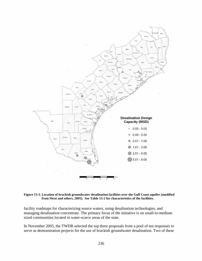
236

Figure 13-3. Location of brackish groundwater desalination facilities over the Gulf Coast aquifer (modified from Nicot and others, 2005). See Table 13-2 for characteristics of the facilities.

facility roadmaps for characterizing source waters, using desalination technologies, and managing desalination concentrate. The primary focus of the initiative is on small-to-medium sized communities located in water-scarce areas of the state.

In November 2005, the TWDB selected the top three proposals from a pool of ten responses to serve as demonstration projects for the use of brackish groundwater desalination. Two of these

237

Table 13-2. Characteristic summary of Texas desalination facilities with capacity ≥0.025 mgd (Modified from Nicot and others, 2005).

Plant Name County

Design Capacity

(mgd) Use Source Startup

Year Process Blending? Disposal Method

SWRA Cameron 6.75 DW GW 2004 RO Yes SWD City of Primera Cameron 2 DW GW 2005 RO Yes SWD City of Raymondville Hidalgo 1 DW GW 2004 RO No SWD

City of Kenedy Karnes 0.72 DW GW 1995 RO Yes SWD City of Seadrift Calhoun 0.52 DW GW 1998 RO Yes SWD Valley MUD #2 Cameron 0.5 DW GW 2000 RO Yes SWD/LA Holiday Beach WSC Aransas 0.15 DW GW 1998 RO Yes SWD

DS Waters of America, LP Waller 0.09 DW GW 1997 RO No SWR

City of Bayside Refugio 0.029 DW GW 1990 RO No EP North Cameron /Hidalgo WA Hidalgo NA DW GW 2005 RO Yes SWD

Total Design Capacity (mgd)

11.76

Notes: DW = drinking water; GW = groundwater; RO = reverse osmosis; SWD = discharge to surface water

body; LA = land application; SWR = discharge to sewer; EP = discharge to evaporation pond; NA = information not available.

projects (North Cameron Regional Water Supply Corporation and City of Kenedy) will be located over the Gulf Coast aquifer. The North Cameron Regional Water Supply Corporation is constructing a brackish groundwater desalination plant that is scheduled to be completed by May 2006. The facility will treat 3.2 mgd of brackish groundwater from the Gulf Coast aquifer and produce a blended output of 5 mgd. The project proponents offer to develop a comprehensive engineering facility roadmap to track the development of the project from start to finish. The City of Kenedy is in the process of retrofitting and modernizing an existing reverse-osmosis groundwater desalination facility and proposes to conduct a feasibility study to add another such facility to meet the city’s projected water needs. The project will allow for a factual comparison of the performance of a new system with the older reverse-osmosis filtration system currently in place. This will result in useful information (cost-benefit) for assessing replacement of similar facilities in other areas of the state.

In anticipation of expected future shortages, four regional water planning groups (regions K, L, M, and N) are recommending brackish groundwater desalination from the Gulf Coast aquifer as a water management strategy to meet these shortages. A short description of these projects follows. All information for the desalination projects within a regional water planning group was obtained from the region’s initially prepared plan submitted to the TWDB for review. The reference to these is cited at the end of the description for each region. It is important to note that these initially prepared plans are still under review by the TWDB and have not yet been approved for inclusion in the 2007 State Water Plan.

238

Region K: The Lower Colorado Regional Water Planning Group (Region K) is recommending a brackish groundwater desalination facility for the STP Nuclear Operating Company in Matagorda County to meet expected shortages in steam electric usage starting in decade 2030. Region K has determined that the Gulf Coast aquifer has a significant volume of brackish water at the STP Nuclear Operating Company location with a TDS concentration of approximately 2,500 mg/l. The brackish groundwater desalination strategy would require the drilling of wells capable of supplying between 40 and 50 mgd (44,800 and 56,000 acre-feet) of brackish groundwater. A plant that is sized to provide 26.4 mgd (29,568 acre-feet) annually will be required. Region K estimates that water from this strategy can be produced for about $430 per acre foot. This is slightly less than one half of the cost of water from a seawater desalination facility (LCRWPG, 2005).

Region L: The South Texas Regional Water Planning Group (Region L) recommends Gulf Coast aquifer brackish groundwater desalination as a water management strategy in Refugio County to provide up to 9.07 mgd (10,160 acre-feet) of additional water annually to the Lower Guadalupe Water Supply Project. The desalination facilities will be located adjacent to the well field and will treat half the brackish water to produce a finished blended water supply that meets all potable water regulatory requirements. After desalination treatment and blending, the finished water from the brackish well field will be delivered to the Lower Guadalupe Water Supply Project transmission system for blending with surface water and other non-brackish groundwater from the Gulf Coast aquifer for delivery to Bexar County. The estimated incremental unit cost to add this supply to the Lower Guadalupe Water Supply Project is $796 acre-feet per year (STRWPG, 2005).

Region M: Based on the success of previous pilot studies and implementation of several projects, the Rio Grande Regional Water Planning Group (Region M) is recommending brackish groundwater desalination as a water management strategy for domestic, municipal, and industrial users in several areas of the region. The proposed desalination projects are expected to have design capacities of between 0.25 and 0.75 mgd (280 and 840 acre-feet). The volume of brackish groundwater required for these projects is expected to total approximately 62,000 acre-feet annually. The annual cost per acre-feet to implement this strategy is estimated to be $506 (RGRWPG, 2005).

Region N: Brackish groundwater desalination is one of 18 water management strategies recommended by the Coastal Bend Regional Water Planning Group (Region N) to meet anticipated shortages in municipal use. The region is recommending this strategy for several cities in Duval County (the cities of Benavides, Freer, and San Diego) and for other water user groups in Live Oak, Jim Wells, Kleberg, and San Patricio counties where brackish groundwater from the Gulf Coast aquifer is readily available. The recommended desalination facilities are relatively small, ranging from 0.6 to 1.2 mgd (672 to 1,344 acre-feet; CBRWPG, 2005).

Conclusions There is an abundance of brackish groundwater in the Gulf Coast aquifer of Texas that is available for desalination. There are, however, difficulties associated with implementing such projects that can be particularly challenging for smaller communities. Chief among them are

239

managing the desalination waste and predicting the long-term performance of brackish groundwater aquifers. Progress is being made on these fronts (for example, work presently being pursued to ease the regulatory burden of desalination waste permitting and modeling the performance of brackish aquifers under pumping conditions) and we are optimistic that, with greater efficiencies offered by modern desalination technologies and continued support from the State, brackish groundwater desalination will play an important role as a source of water supply in the future.

References Ashworth, J. B., and Hopkins, J., 1995, Aquifers of Texas: Texas Water Development Board

Report 345, 69 p.

CBRWPG, 2005, Initially prepared regional water plan: Coastal Bend Regional Water Planning Group, Available at (http://www.twdb.state.tx.us/rwpg/2005_1PP/Region%20N/ Volume%20I/Section%204B.pdf).

Kalaswad, S., Christian, B., and Petrossian, R., 2004, Brackish groundwater in Texas, in Arroyo, J., editor, The Future of Desalination in Texas, Volume II: Texas Water Development Board Report 363, p. 9–21.

LBG-Guyton Associates, 2003, Brackish groundwater manual for Texas regional water planning groups: Contract report prepared for the Texas Water Development Board, Austin, Texas, 188 p. Available at (http://www.twdb.state.tx.us/RWPG/rpgm_rpts/2001483395.pdf).

LCRWPG, 2005, Initially prepared Region “K” water plan for the Lower Colorado Water Planning Group: Lower Colorado Regional Water Planning Group. Available at (http://www.twdb.state.tx.us/rwpg/2005_1PP/Region%20K/Chapter%204.pdf).

Nicot, J.-P., Walden, S., Greenlee, L., and Els, J., 2005, A desalination database for Texas: Report prepared for the Texas Water Development Board, Austin, Texas, 35 p. Available at (http://www.twdb.state.tx.us/RWPG/rpgm_rpts/2004483021_Desal_Database_Texas.pdf).

RGRWPG, 2005, Initially prepared plan: Rio Grande Regional Water Planning Group Available at (http://www.twdb.state.tx.us/rwpg/2005_1PP/Region%20M/Chapter%204%20IPP.pdf).

SCTRWPG, 2005, Initially prepared 2006 regional water plan: South Central Texas Regional Water Planning Group Available at (http://www.twdb.state.tx.us/rwpg/2005_1PP/Region%20L/Volume%20II/ Summary%20Sheets/Summary%20Sheet%204C.21%20Gulf%20Coast.pdf).

TCEQ, 2004, Drinking water standards governing drinking water quality and reporting requirements for public water systems: Texas Commission on Environmental Quality, 30 TAC Chapter 290, Subchapter F: TCEQ RG-346, 99 p.

TWDB, 2002, Water for Texas—2002 State Water Plan: Texas Water Development Board, v. 1, 155 p. Available at (http://www.twdb.state.tx.us/publications/reports/State_Water_Plan/ 2002/FinalWaterPlan2002.asp).

Warner, D. L., 2001, Technical and economic evaluations of the protection of saline ground water under the safe drinking water act and the UIC Regulations: Report submitted to the

240

Ground Water Protection Research Foundation, 44 p. Available at (http://www.gwpc.org/uic/ State_App3.pdf).

241

Chapter 14

Brackish Groundwater Desalination in South Texas: An Alternative to the Rio Grande

Joseph W. (Bill) Norris, P.E.1

Growing Concerns In the mid-1980s, this author began looking at the potential for utilizing brackish groundwater to supplement the over allocated Rio Grande. It has been done for years in Florida. Why can it not be done in the Rio Grande Valley? In 1988, a trip to look at existing brackish groundwater facilities was made by the Brownsville Public Utilities Board to see what was involved to construct and operate this type of facility. While this process had merit, the mild drought was relieved later in the decade. In the mid-1990s, the Rio Grande Valley was experiencing what would ultimately end up as the drought of record, ending in 2004. Brownsville was yet again interested in pursing this option a little closer, since Brownsville is the last to take water from the Rio Grande after release from the Falcon Reservoir. Much of this water is lost to evaporation, seepage and theft, especially in times of drought. There was some concern, but not desperation, to pursue the alternative to desalinate brackish water.

In 1984, a matching grant was awarded to the Brownsville Public Utilities Board to study the feasibility of providing desalinated brackish groundwater to Brownsville, thus beginning what has been a rapidly growing industry in South Texas.

Regional Planning Efforts

Brackish Groundwater Resources

What was once an unusable supply is now becoming a cost effective means of providing alternative water resources to water user groups. In the Rio Grande regional water planning area (Region M), there are two main aquifers that can yield sufficient quantities of brackish groundwater. Of course, additional treatment will be required, such as reverse osmosis or electrodialysis reversal, to remove total dissolved solids. The aquifers that would supply this brackish water are the Gulf Coast aquifer and the Carrizo-Wilcox aquifer.

1 NRS Consulting Engineers

242

The Gulf Coast aquifer system may be an excellent source of brackish groundwater in many areas. The southern/western portion of the aquifer system is the best brackish groundwater resource because of the dominance of groundwater high in total dissolved solids. In addition, the aquifer system may be an excellent brackish groundwater resource in other areas, in particular in several areas at or near the coast where poor water quality is common.

Brackish Desalination Demand

Based on responses to a survey sent to 63 water user groups in the Rio Grande regional water planning area, the use of brackish groundwater desalination is a strategy that they will be using now and into the future. Thirty of the 44 respondents indicated that they would be pursuing this water management strategy within the next 2 years. They could not wait until the next planning cycle to be included. Over 56,000 acre-feet of brackish ground water is expected to be used over the next 50 years.

Demand for this strategy can be attributed to the reduction of costs, education on desalination, cost of surface water rights, security, and reduction of surface water availability. Projections for this strategy are to be implemented by 2010 but are only projected to remain constant through 2050. Further water supply availability will be studied during the current planning cycle to evaluate increases from the year 2010.

Description of Brackish Desalination Desalination of brackish groundwater is most commonly accomplished through reverse osmosis. A full-scale reverse osmosis system to treat brackish groundwater would require pretreatment, which would include a cartridge filtration system to remove minimal suspended solids. Acid and a silica scale inhibitor would also be added to prevent scale formation. A full-scale system would be expected to have a membrane life of approximately five years. Chemical cleaning of the membrane would be required approximately one to four times per year. The results of the Valley Municipal Utility District plant indicate that larger reverse osmosis systems treating brackish groundwater successfully meet all state and federal primary and secondary drinking water standards.

Concentrate from the reverse osmosis system must be disposed of in an environmentally acceptable manner. Most of the current or proposed systems will utilize drainage ditch discharge, which ultimately will discharge into the Laguna Madre or the Gulf of Mexico. Other options include disposal to a sewer system and deep well injection.

History of Desalination in South Texas After the Brownsville Public Utilities Board’s initial review of the potential of treating desalinated water in 1988, a dedicated interest was not present until 1994, when the Brownsville Public Utilities Board pursued the joint feasibility project with the Texas Water Development Board (TWDB). There was, however, a major desalination project that did not include brackish groundwater but utilized wastewater effluent as the source water. Since the initial Valley

243

Municipal Utility District Plant, there has been substantial development of brackish groundwater treatment plant in the Rio Grande Valley. These developments are listed and described further below:

• 1990 Harlingen wastewater desalination plant

• 1995 Brownsville/Texas Water Development Board brackish desalination feasibility/pilot study

• 1996 LMWD/ Texas Water Development Board sea-water feasibility/pilot study

• 1999 Valley Municipal Utility District first potable brackish desalination plant constructed

• 2001 Southmost Regional Water Authority feasibility study

• 2003 Regional Water Planning Group plan amendment

• 2003 Multiple facilities in planning/design

• 2004 Southmost Regional Water Authority and North Alamo Water Supply Corporation/La Sara regional desalination plant in production

• 2005 North Cameron Regional Desalination Plant under construction

• 2005 North Alamo Water Supply Corporation /Edinburg North and South Plant in design phase

Harlingen Fruit of the Loom

While this project does not utilize brackish groundwater, it highlighted the use of reverse osmosis treatment to desalinate the wastewater into high quality water to be utilized in the manufacturing process to produce textiles. This highly recognized project brought to light the use of the reverse osmosis process as a feasible alternative to conventional treatment methods. It is this author’s opinion that this project was the catalyst to develop the desalination of brackish water to come in subsequent years.

When this project was initiated, Fruit of the Loom was considering Harlingen as a viable location for their bleaching and dying operation and the creation of 2,000 jobs. Obstacles included the quality of the water to be provided and the cost. The drinking water was too high in total dissolved solids, mainly carbonate hardness. If the company were to take this water, further treatment would be required, and thus additional costs added, to what was considered an already high cost of water (over $1.20 per 1,000 gallons). This cost did not include wastewater service.

Another alternative was to consider the use of water from the Arroyo Colorado and water from the Rio Grande via the Harlingen Irrigation District. These two alternatives proved to be too costly due to the level of treatment required.

The idea of utilizing wastewater was evaluated as a viable option. The initial cost of water was free from the wastewater plant and was not used for any other purpose. The water was of good quality compared to Rio Grande or Arroyo Colorado water sources. Considering the cost of treatment, it was less costly to treat to the level needed using wastewater effluent than any other

244

source available at the time. The initial cost charged to Fruit of the Loom was $1.20 per 1,000 gallons for both water and wastewater service. The City of Harlingen also constructed a separate facility to treat the industrial wastewater returned to the wastewater plant. The industry shut down operations in Harlingen in 2003. At that time the use of effluent reuse was no longer utilized for this or any other purpose due to lack of demand.

Feasibility Studies

During the initial stage of the drought of record in the Rio Grande Valley, a great deal of interest was given to alternative sources of water, mainly brackish and seawater desalination. In 1985, the Brownsville Public Utility Board and Texas Water Development Board teamed together and authorized NRS Consulting Engineers (NRS) to prepare a feasibility study to take brackish groundwater in the Brownville area and treat it through reverse osmosis or electrodialysis reversal. Results of this study indicated a very good possibility of treating up to 20 million gallons per day (mgd) of brackish well water to serve the Brownsville area. Much was dependent upon subsequent well testing to firm up the supply numbers from previous well drilling in the area. The data from well drilling in the area was quite sparse, as very few entities utilize groundwater for their sources of water in this area.

Results of this study, completed in 1996, are shown in Table 14-1.

Valley Municipal Utility District No. 2 Desalination Plant

The Valley Municipal Utility District No. 2 made a large step in securing its future water supply by utilizing brackish water wells. The district, which provides water service to Rancho Viejo and River Bend Resorts, completed the valley’s first municipal reverse osmosis treatment plant in 1999. This 250,000-gallon per day facility provides bottle quality water to its customers while preserving their water supply.

The project was completed utilizing NRS to provide the pilot testing, permitting, design, and construction management. By utilizing the construction management procedure, the district realized over 30 percent savings over conventional construction procedures. The total project costs for construction were $715,000, as compared to the conventional bid price of $940,000. Detailed costs are shown in Table 14-2.

Southmost Regional Water Authority

The Southmost Regional Water Authority (Authority) is a conservation and reclamation district created in 1981 and organized pursuant to Article XVI, Section 59 of the Texas Constitution. Its mission is to provide the most cost-effective and reliable alternative water supply to its members. The Southmost Regional Water Authority’s operating history began in 2000, when it was activated to address long-term regional water supply issues in the southern Cameron County region. The project provides for a blended output of 7.5 mgd and is allocated as shown in Table 14-3.

245

Table 14-1. Brownsville feasibility study projection of costs (1996 dollars).

Demonstration of tangible success

The key to successful completion of this project was a direct result of communication. The following is a list of items that were implemented to complete the project.

Regional approach—A regional approach brings difficulties in coordination between political bodies. The only negative aspect to this approach is the feeling of losing control of the entity’s destiny. This happened to the Laguna Madre Water District, an original project participant. They opted out of participation in the final project. For the most part, if a feeling of cooperation can be maintained through Authority leadership, the regional process has great advantages to all members, including capital and operation cost benefit economies of scale. Leadership of the Authority was instrumental through two chairmen, Robert H. Lackner and Billy R. Bradford, Jr.

246

Table 14-2. Valley Municipal Utility District construction costs (1999 dollars).

Table 14-3. Southmost Regioanl Water Authority water allocation.

Allocation of water sales (Based on 2001 annual water sales) Available capacity from Authority 7.5 mgd Water supply,

mgd Entity Water Sales Percent Brownsville Public Utilities Board 5,869,000,000 92.91% 6.9681 Valley MUD No. 2 158,545,873 2.51% 0.1882 City of Los Fresnos 143,981,700 2.28% 0.1709 Brownsville Navigation District 132,536,000 2.10% 0.1574 Town of Indian Lake 12,935,000 0.20% 0.0154

Mr. Lackner pushed for the planning and construction of the facility, and Mr. Bradford lead through the construction and start-up of the facility.

Construction management—Construction management of the design and construction of the plant has great advantages for control and cost savings of the facility. It is expected that over $4,000,000 was saved with this approach. Drawbacks include additional coordination efforts and potential for “finger pointing” of any problems. Proper contract by construction discipline (such as civil, mechanical, electrical, etc.) and communications minimized these potential difficulties. For time management, change orders were issued to contractors on site to accomplish additional work. Actual bidding of every aspect would not have accomplished the time and cost goals of the project. Typically with this process change, orders are not for errors or omissions but for additional work required to finalize the project.

Weekly planning, design, and operation meetings—The single most important aspect to the success of this project was a result of communications from the beginning of the project development. The owner’s representatives were involved in planning, design, construction, and operations of the plant. This provided for valuable input and pride of ownership of the team.

Timeline—An aggressive timeline was established early in the project. At the time of design, there was a desire to have treated water within 18 months. Major portions of the project design and bidding were completed in the summer of 2002. Funding was not in place until December

Building $64,039 Reverse Osmosis System, Chlorination, Electrical and Instrumentation

$450,000

Offsite Utilities $89,800 Well/Pumps $100,498 Site Work $9,987 Total $714,324 Plant Capacity, gallons 250,000 Value of Water Rights Saved @ $1,500/acre-feet

$409,500

247

2002. Contracts initiation could not be issued until January 2003. Additional delays for property acquisition delayed the well field completion and subsequent projects. Heavier than normal spring and summer rains helped to delay some of the well completions. In spite of external difficulties, initial project start-up was approximately 14 months after initiating construction. Final start-up and operation took an additional six months. Realistic timelines should be communicated with the owner to eliminate unrealistic expectations and disappointments.

Project layout—The plant site is situated on a 17-acre site, suitable for multiple cost effective expansions. A smaller site plan could be used if conventional methods of construction were used. Facilities were laid out to allow construction room for multiple contracts. Inside the plant building, additional room for expansion and maneuverability were keys to the current and future ease of operation.

State permitting—Permitting through the Texas Commission on Environmental Quality took about eighteen months. Delays were due to the inexperience of the Texas Commission on Environmental Quality in reviewing permits of this type. Continuous communication and education helped to move the process along. Objections to the permit by non-affected parties added several months to the process. The permitting process is the longest lead-time item to consider. Another issue is that this is considered an industrial wastewater discharge and all that it implies. Work should take place to properly classify this as a water treatment by-product. Permitting steps should be one of the first things to start in the planning process.

Land and rights of way—Land acquisition can be both expensive and time intensive. Once the word gets out of a public entity in pursuit of property, cost escalates. Negotiations were completed for this project successfully, but took substantial time. This, along with the permitting process, should proceed as soon as possible. Options should be pursued in case well testing does not prove suitable sites.

Partial start-up—Due to large lines sized for full start-up and future supplies, low velocities on partial start up create certain opportunities not present under full operations. There do not seem to be many ways around this problem if partial supply is needed. Perhaps better timing of bringing all facilities on line simultaneously could be a goal, but for the most part this would have to be an ideal situation, considering multiple contractors each having their own construction issues.

Construction meetings—Even though there were 15 construction contracts, monthly meetings were held to discuss accomplishments, schedules, and issues related to construction. The project provided for an on-site professional engineer, three project representatives, a part time technician, and graduate engineers. This procedure of monthly meetings should be implemented for all projects of this type.

Local permitting—Overlooked as a requirement, the local ordinance required that the Authority apply for an industrial waste discharge permit to dispose of the backwash cleaning solution to the Brownsville Public Utility Board’s wastewater treatment facilities. This minor amount of water, meeting all quality requirements, was subject to an application process that rivaled that of the state’s concentrate disposal application. Developers of future projects should be aware of local permitting conditions, even though they are the beneficiaries.

248

Goals—At the onset of a project of this type and magnitude, set realistic goals for completion with proper projections of costs. This project set high goals to complete in 14 months but certain delays should be expected. These include funding, rights of way, permitting, weather, and construction difficulties. Six to 12 months should be allowed for start-up and the development of operational standards, especially if this is the first facility of this type for an organization.

Conclusions—The project is a huge success. This does not mean there is no room for improvements on issues that arise. Accomplished was a regional desalination plant that provides each entity with over 40 percent of their current water supply, supplementing the water from the Rio Grande. This is done to diversify resources for dependability. The newfound source of water is of highest quality and is provided at costs comparable to those of conventional surface water treatment. Oversized facilities will provide cost effective expansions in the future.

North Alamo Water Supply Corporation—La Sara Project

The North Alamo Water Supply Corporation provides water service to rural areas in Hidalgo, Willacy, and Cameron counties. The La Sara project, planned in 2003 to replace the original surface water plant nearby, was completed in 2004. This 1.0 mgd (blended 1.25 mgd) facility services the northeast portion of Willacy County, including La Sara, Port Mansfield, and San Perlita.

Construction of this facility was completed using multiple contracts and managed by NRS. In-kind services provided by North Alamo Water Supply Corporation aided in making this project highly cost effective, especially considering its size. Existing ground storage and pumping facilities were utilized, reducing the cost of this facility. Total construction cost was less than $2.2 million and is described further in Table 14-4.

By utilizing brackish groundwater, the North Alamo Water Supply Corporation realized a surface water savings of over 1,120 acre-feet. Current value of surface water rights is $2,000 per acre-foot. The value to North Alamo Water Supply Corporation is over $2.2 million, or an amount equal to the project cost of the facility.

North Cameron Regional Water Project

The entities of North Alamo Water Supply Corporation, East Rio Hondo Water Supply Corporation, and the City of Primera teamed together to plan and construct a regional shared brackish groundwater treatment plant. The group initiated testing of the groundwater conditions for this project in 2003. Results indicated that a good supply of brackish water was available from the Gulf Coast aquifer located in Northwest Cameron County, west of the City of Primera. The project is currently under construction, with projected completion in May 2006. Table 14-5 further describes the cost of the project.

The projected final construction cost for this 2.0 mgd (2.5 mgd blended) brackish desalination plant is $5.9 million. Unlike the La Sara project, this project is not located near existing ground storage and pumping facilities or offsite distribution. These are included in the project cost. Upon completion, this project will save the regional participants over 2,800 acre-feet of water rights

249

Table 14-4. La Sara Project costs.

North Alamo Water Supply Corporation Reverse osmosis process (two trains of 0.5 mgd each)

Description Contractor Cost Land purchase NAWSC $50,000 Test wells J&S Water Wells $40,000 R.O. building and concrete containment Haraway Cont. $169,393 R.O. system AES $957,148 Electrical Metro Electric $340,443 SCADA Trac & Trol $5,000 Well development J&S Water Wells $377,063 Fencing Kanaf $7,000 Site work NAWSC $5,000 Paving $18,500 Concentrate line (415 L.F. @ $15/L.F.) NAWSC $6,225 Well line (146 L.F. @ $15/L.F.) NAWSC $2,190 Ditch crossing casing and installation NAWSC $5,000 Ditch crossing piling Oden Contractors $9,500 Product water line to ground storage (200 L.F. @ $15/L.F.)

NAWSC $3,000

Subtotal Project Construction $1,995,462 Engineering/Const Mgmt Preliminary engineering/permitting/pilot testing $26,500 Laboratory testing $5,000 Design engineering $82,500 Construction management $75,000 Start up/training $8,250 Subtotal Engineering/Const Mgmt $197,250 Total Project Costs $2,192,712

annually at a capital value of $5.6 million. Each participant is contracted for an equal share of the output of the plant.

North Alamo Water Supply Corporation/Edinburg

North Alamo Water Supply Corporation has two surface water treatment plants, located northeast and southeast of Edinburg, and provides wholesale treated water to the City of Edinburg. Currently under design with projections for construction in Spring 2006 are two 3.0 mgd (3.5 mgd blended) brackish desalination plants located at each of these existing surface water plants. Test wells were drilled in the Gulf Coast aquifer to confirm the supply source of brackish water. Total projected cost for each plant is $5.9, million for a total of $11.8 million for 7.0 mgd blended capacity. This yields 7,840 acre-feet of surface water rights savings at capital value of over $15.6 million.

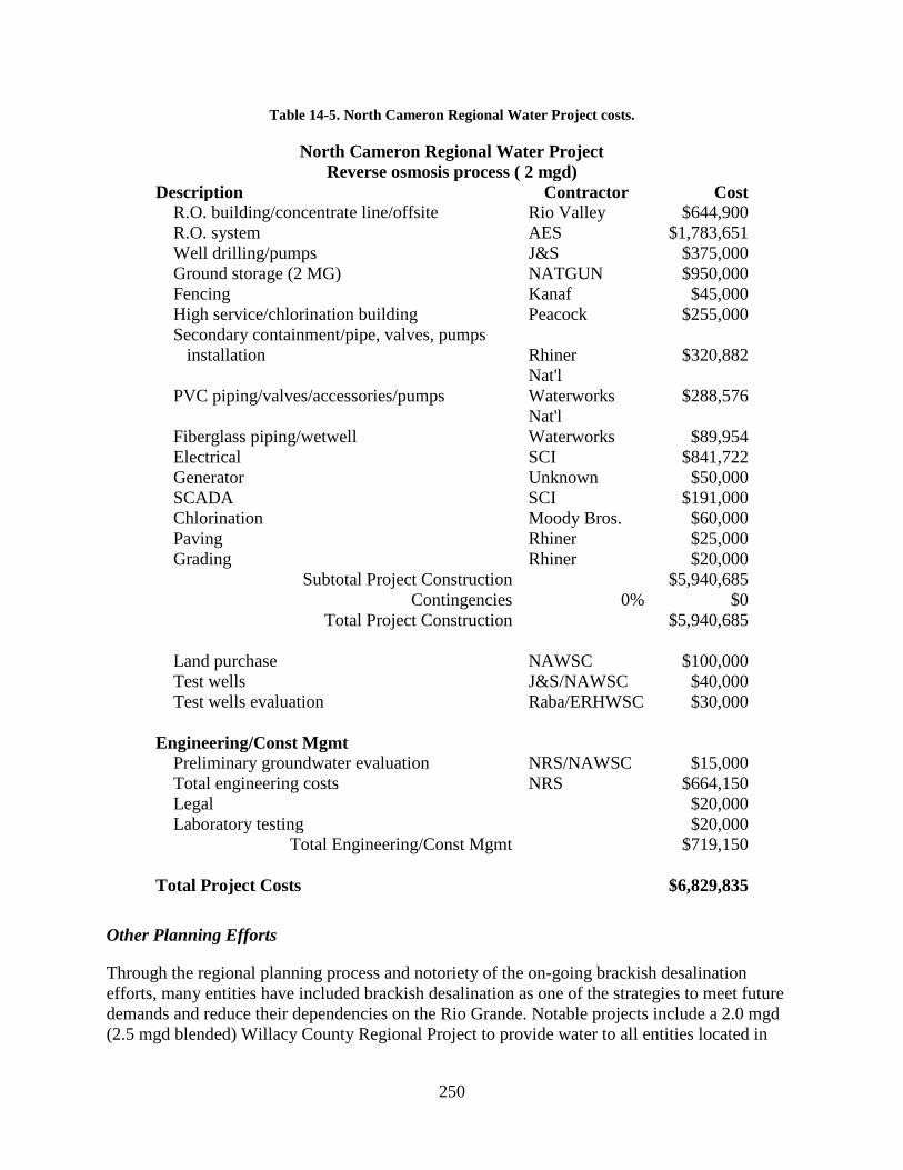
250

Table 14-5. North Cameron Regional Water Project costs.

North Cameron Regional Water Project Reverse osmosis process ( 2 mgd)

Description Contractor Cost R.O. building/concentrate line/offsite Rio Valley $644,900 R.O. system AES $1,783,651 Well drilling/pumps J&S $375,000 Ground storage (2 MG) NATGUN $950,000 Fencing Kanaf $45,000 High service/chlorination building Peacock $255,000 Secondary containment/pipe, valves, pumps installation Rhiner $320,882

PVC piping/valves/accessories/pumps Nat'l Waterworks $288,576

Fiberglass piping/wetwell Nat'l Waterworks $89,954

Electrical SCI $841,722 Generator Unknown $50,000 SCADA SCI $191,000 Chlorination Moody Bros. $60,000 Paving Rhiner $25,000 Grading Rhiner $20,000

Subtotal Project Construction $5,940,685 Contingencies 0% $0

Total Project Construction $5,940,685

Land purchase NAWSC $100,000 Test wells J&S/NAWSC $40,000 Test wells evaluation Raba/ERHWSC $30,000

Engineering/Const Mgmt Preliminary groundwater evaluation NRS/NAWSC $15,000 Total engineering costs NRS $664,150 Legal $20,000 Laboratory testing $20,000

Total Engineering/Const Mgmt $719,150 Total Project Costs $6,829,835

Other Planning Efforts

Through the regional planning process and notoriety of the on-going brackish desalination efforts, many entities have included brackish desalination as one of the strategies to meet future demands and reduce their dependencies on the Rio Grande. Notable projects include a 2.0 mgd (2.5 mgd blended) Willacy County Regional Project to provide water to all entities located in

251

Willacy County. Discussions have taken place for desalination possibilities with the City of McAllen also. If an entity has a choice between a surface water supply and brackish groundwater supply, it behooves them to evaluate the alternatives.

Cost Factors in Desalination

Total Dissolved Solids

The degree of TDS is a good general indication of what it will cost to remove TDS to meet drinking water standards. The higher the TDS, the higher capital, operation, and maintenance costs. For example, a 3,000-TDS feed water could yield 80 percent (8 out of 10 gallons supplied) where as a seawater plant at 35,000 TDS feed water would only yield around 45 percent, thus increasing the size of the units. Pressures to remove the lower TDS level is only 180 psi, compared to upwards of 900 psi for the seawater, an obvious increase in power costs.

Power Costs

Power cost account for around 40 percent of the operational costs of a facility. Work is being implemented to recover excess pressures during the process. Investigation into off-peak power contracts would be helpful in controlling the ultimate cost of the facility.

Location

Not all locations will be of equal cost. One of the major factors is the ability to discharge the concentrate generated at the plant. Coastal communities have a great advantage over inland communities. The location of the facility near the well field and distribution system will also enhance the attractiveness of this alternative.

Economies of Scale

If entities can work together to construct regional facilities, they can reap the rewards of lower unit cost for construction and lower operational costs by building less facilities with less manpower.

Construction Method

Construction management of multiple contracts in South Texas has resulted in as much as 30 percent savings over convention construction methods. General construction contracts will normally be higher, due to the lack of local experience in this field.

252

Water Treatment Trends Based on our experience, there has been a downward trend in costs to construct brackish and seawater desalination plants, due to technology advances in the industry over the years. Conversely, with increasing regulations in drinking water standards, the cost to treat surface waters has been increasing. The degree of contaminant removal through RO compared to conventional filtration is much greater with RO. Consideration should be given to these alternative methods when evaluating additional treatment capacity needs.

Replicating Success The success of an initial concept or project is the ability of the project build to support and provide for a model for subsequent projects that continue to improve. The concept of brackish desalination started conceptually in the mid-1990s. Over the last 5 years, projects have been designed and/or implemented to provide over 17 mgd of additional high quality treated water, or over 19,000 acre-feet of additional water supply. This equates to a water rights cost savings of over $47 million. Educating the public on the cost effectiveness is a key to further the completion of similar facilities.

Innovation The use of brackish groundwater is innovative in South Texas, as it is using a water supply that was once deemed useless and quite uncommon in Texas, even though Florida has been treating water this way for many years. State-of-the-art technology is used to treat and monitor project components.

The implementations of the projects have been innovative, beginning with the Valley Municipal Utility District project. The use of multiple projects by construction discipline has been used successfully on all projects completed in South Texas. In these cases, the engineer acts somewhat as a general contractor, but bids as many as 20 contracts per project and controls the coordination between contractors without the markup normally placed on the purchase of equipment and subcontractors. Because of the nature of the construction, there are very few local or state contractors familiar with the construction of these types of facilities. This method has yielded savings upward of 30 percent over conventional methods of construction. Owners should understand that the savings gained increases the shared responsibility of project success between the owner and the engineer.

All projects have been implemented with one or more partners, thus creating an economy of scale and saving additional construction and operation dollars for each participant.

Water Supply Only recently has there been substantial well testing and monitoring in South Texas. With the implementation of several projects, we will be able to better monitor and define aquifer

253

characteristics. This is important in determining the ultimate yield of the aquifer. Most wells were drilled in the 1950s, during a major drought, but have not been used due to their brackish nature. Brackish groundwater cannot be used for irrigation, so demand would be only for municipal use.

Issues to be Addressed We need to continue working in several areas to improve the success of brackish desalination. The growing concern of concentrate disposal is primary on the list and more important to inland communities without the ability to discharge into a salt water body along the coastal areas.

Because power accounts for 30 to 50 percent of operational costs, technology advances in power savings through energy recovery, fuel cell development, and renewable sources should be pursued.

Conclusions We must realize that all sources of water are limited and we must use them wisely and efficiently. Seawater provides the most unlimited source of water but most often carries the highest cost to implement. Brackish water has shown to be a viable alternative to the limited surface water supplies in South Texas. From the initial feasibility studies starting in 1995 to the largest brackish groundwater facility in Texas to date, this is a growing industry and is expected to grow into many areas of the state to account for increasing demands and decreasing supplies.

The use of brackish desalination is not for everyone and will not take the place of surface water. What it will be is an opportunity for entities to provide a reliable water alternative and diversify the supplies while improving water quality in the process.

254

This page intentionally blank.

255

Chapter 15

Effects of Oil and Gas Production on Groundwater

John James Tintera, P.G.1 and Leslie Savage, P.G.1

Introduction The Railroad Commission of Texas (RRC) has the statutory authority and duty to regulate a wide range of oil and gas operations for the purpose of conserving resources, protecting correlative rights, and protecting the state’s water resources.

Section 91.101 of the Texas Natural Resources Code provides the RRC with jurisdiction over the full scope of oil and gas exploration, development, and production operations and activities, including the drilling of wells associated with oil and gas activities, gas plants, natural gas or natural gas liquids processing plants, pressure maintenance plants, underground hydrocarbon storage facilities, and activities associated with the storage, handling, reclamation, gathering, transportation, or distribution of oil or gas. In addition, under Section 26.131 of the Texas Water Code, the RRC is solely responsible for the control and disposition of waste and the abatement and prevention of pollution of surface and subsurface water resulting from oil and gas activities.

To meet its statutory responsibilities, the RRC has adopted regulations to prevent contamination of surface water and groundwater from oilfield activities and has established programs to abate such contamination when it does occur.

Regulatory History Texas has been producing oil for more than 100 years and has had regulations applicable to oilfield pollution prevention since 1899.i Such regulations include requirements and standards for well construction, integrity testing, and plugging, as well as pollution prevention, spill response, and oil and gas waste management. The RRC’s pollution regulations have evolved significantly since those early days, even before the elevation of our national environmental conscience, which some say began with the 1962 publication of Rachel Carson’s Silent Spring.

For example, Texas once allowed disposal of produced water in earthen evaporation pits and surface waters. The State recognized this as a potential problem back in the 1950s, and the RRC

1 Railroad Commission of Texas

256

began prohibiting such pits and discharges on an area-wide basis starting in 1955.ii In 1969, the RRC prohibited such pits and discharges statewide.iii

Another example of the RRC’s evolving environmental regulations is the history of the RRC’s well plugging requirements and programs. Although legislation was passed in 1899 concerning the plugging of oil and gas wells, the Texas Legislature gave no agency specific responsibility for enforcing the plugging of inactive oil and gas wells until 1919, when it authorized the RRC to enforce the laws.iv Since 1919, the RRC has had rules on plugging abandoned wells to confine oil, gas, and associated saltwater to the strata in which they originated. The drought of the 1950s focused Texas’ attention on the need to better protect clean water. In 1957, with more knowledge of the nature of subsurface water, standards for plugging were revised to ensure greater protection of groundwater.v

Today, the RRC has even greater control of the proper plugging of abandoned wells and waste management practices through enhanced inspection and enforcement mechanisms and personnel, an ability to administer administrative penalties of up to $10,000 per day per violation, a greater ability to track the status of wells and other operations through computer databases, and financial security requirements for operators.vi

Additional RRC programs serve to ensure protection of groundwater. In 1982, the U.S. Environmental Protection Agency (EPA) delegated to the RRC the Underground Injection Control program under the federal Safe Drinking Water Act for that portion of activities under the RRC’s jurisdiction. Currently, there are approximately 49,911 Class II permitted and active injection and disposal wells, 359 active hydrocarbon storage wells, and 84 Class III active brine mining wells in Texas. The RRC tracks injection pressures and volumes for each of these wells annually. The RRC also receives and reviews approximately 17,000 mechanical integrity pressure tests annually from oilfield operators.

In 1984, the RRC further strengthened its environmental regulations by adopting major amendments to its regulations concerning pit and surface waste management standards (Rule 8), including standards for short-term pits such as drilling pits and completion/workover pits.vii The rule authorizes some short-term, relatively low risk waste management practices and requires permits for other waste management practices. The rule prohibits a person conducting activities subject to RRC regulation from causing or allowing pollution of surface or subsurface water in the state.

The RRC has an extensive monitoring and enforcement program, which acts to detect and correct problems in the field. The RRC’s Field Operations section is responsible for ensuring statewide compliance by oil and gas operators of the regulations of the RRC. The state is divided into nine districts, with an office located in a key city in each district. The RRC’s district personnel are the first responders to spills, blowouts, fires, sour gas releases, and other oilfield-related emergency operations. Approximately 88 field inspectors and lead technicians are responsible for a total of 358,746 wells. Field Operations performs inspections based on a priority system that places an emphasis on jobs and activities that pose the greatest risk to public safety or the environment. In fiscal year 2005, Field Operations performed over 115,000 jobs consisting of inspections and/or monitoring of oilfield activities.

257

Oil Field Cleanup Program Review However, as in any industrial activity, equipment can fail and employees may err, and groundwater pollution may result. Under the Oil Field Cleanup Program, the RRC has established multiple pollution abatement programs that complement each other. These programs include a Well Plugging Program to plug abandoned wells, a State Managed Cleanup Program to assess and clean up abandoned oil and gas sites, an Operator Cleanup Program to oversee responsible operator cleanup, and a Voluntary Cleanup Program designed to encourage developers, landowners, or other innocent parties to identify and clean up oilfield pollution. Details about these programs are available on the RRC web site at http://www.rrc.state.tx.us/. The programs are funded through a variety of mechanisms, including operator filing fees, regulatory fees on oil and gas production, penalties, and collections on financial security instruments.viii In addition, the RRC has leveraged these funds with millions of dollars of other state and federal grant funds.

Funding In 1965, the Texas Legislature created a Well Plugging Fund to assist in the plugging of a polluting well for which no operator could be found; however, biennial appropriations were required, and appropriated funds were less than what was needed to fully address the problem.ix In 1983, the Legislature provided the RRC with administrative penalty authority and application fees to fund the Well Plugging Fund as well as an increased budget for additional legal, administrative, and field staffing.x The RRC also imposed plugging deadlines and financial security requirements on oil and gas operators.

In 1991, the Legislature replaced the Well Plugging Fund with an expanded Oil Field Cleanup Fund to plug abandoned wells as well as to clean up pits and other sites associated with oil and gas operations. This fund, the legislation for which was supported by the Texas oil and gas industry, is supported by fees, penalties, and other payments collected from the oil and gas industry.xi The RRC leverages this fund with various state and federal grants. Since the RRC implemented the Well Plugging Program in 1984, the RRC has plugged over 24,000 abandoned wells. Since the initiation of the Oil Field Cleanup Program in 1992, the RRC has completed over 3,000 clean up activities at abandoned sites with state-managed funds. The abandoned wells to be plugged and sites to be cleaned up are prioritized based on the risk to public safety or the environment.

Pollution Cleanup RRC regulations require that responsible operators clean up pollution caused by oil and gas activities. The RRC considers groundwater pollution cleanup requirements on a site specific, case-by-case basis. The RRC allows the responsible operator to select the remediation technique as long as clean up is effective and timely. Currently-accepted federal or state remediation protocols are applicable, and acceptable cleanup standards are consistent with federal and state drinking water standards unless aquifer characteristics and land use controls allow for alternate cleanup levels.

258

Pollution Sources A variety of oilfield materials can impact groundwater. These include produced saltwater, drilling fluids, and associated wastes such as well treatment chemicals, crude oil, and hydrocarbon condensate. Produced water constitutes about 98 percent of all oil and gas waste; however, in Texas over 99 percent of all produced water is injected in wells regulated under the RRC’s Underground Injection Control program. Drilling fluids and associated oil and gas wastes make up about 1.6 percent and 0.4 percent by volume of oil and gas waste, respectively.xii

Groundwater quality has been impacted by past practices (now prohibited), accidental spills, pipeline leaks, blowouts, and situations that are noncompliant with current RRC regulations. Contaminants released as a result of these situations can include dissolved salts from produced water; barium from drilling fluids; hydrocarbons from crude oil and natural gas condensate, as well as other heavy metals; and refined hydrocarbons and chemicals from well treatment fluids.

Interagency Cooperation The RRC is one of ten members of the Texas Groundwater Protection Committee (TGPC), which was established in 1989 by the Texas Water Code, Chapter 26, Subchapter J, relating to Groundwater Protection.xiii The purpose of the TGPC is to coordinate groundwater protection activities across Texas. TGPC duties include publishing an annual groundwater monitoring and contamination report, updating the state groundwater protection strategy, and reporting to the Texas Legislature on groundwater protection activities and recommendations for groundwater legislation. The TGPC’s annual report for 2004, entitled “Joint Groundwater Monitoring and Contamination Report for 2004,” lists a total of 6,746 active documented groundwater contamination cases from all sources. Of those 6,746 cases, 241, or approximately 3.6 percent of all active, documented cases, were related to oilfield activities. Over 230 cases in which the probable source of contamination was related to oilfield activities have been closed since the RRC began reporting such cases in 1989.

It is interesting to note that of the closed documented groundwater contamination cases related to oilfield activities under the RRC’s jurisdiction, the contaminant was salt and/or hydrocarbons in 222, or approximately 97 percent, of the cases. The remaining eight cases included other contaminants, such as metals (barium, mercury, and chromium), hydrochloric acid (HCl), glycol, polychlorinated biphenyls (PCBs), and sulfates.

Conclusion There has been oil and gas activity in Texas since 1866, when Lynis T. Barrett drilled the first producing Texas well in Nacogdoches County.xiv From the beginning, the RRC has exercised its statutory authority to enact regulations to protect surface and subsurface water and has vigorously enforced those regulations to ensure compliance. In the last few years, the RRC has broadened and enhanced its ability to prevent pollution through strengthening its regulations and enforcement and to abate pollution of groundwater with numerous complementary programs that are funded by the oil and gas industry. As oil and gas exploration and development

259

methodologies become more sophisticated, so too does the concomitant need for environmental protection, assuring that, as new plays and higher prices drive additional oilfield development, groundwater and other resources of Texas are preserved and protected.

References i Texas House, 1899, House Bill 542, 26th Texas Legislature, regular session. Ch. 49, Tex Gen Laws 68.

ii Special Order Pertaining to Disposal of Salt and Sulphur Water Produced Incident to the Production of Oil and Gas In the Rodman-Noel (Grayburg) Field, Upton County, Texas, Oil and Gas Docket No. 7-32,629, December 19, 1955.

iii Special Order Amending Rule 8 of the General Conservation Rules of Statewide Application, Oil and Gas Docket No. 20-56,841, April 3, 1967 (effective January 1, 1969).

iv Rule 20, Oil and Gas Circular No. 7, June 18, 1919, (available) at the Railroad Commission Library and the University of Texas Center for American History.

v Memorandum to District Supervisors, May 30, 1957 (available) at the Railroad Commission Library, (codified as Rule 15, effective June 1, 1964).

vi Railroad Commission of Texas, Statewide Rules, 16 Tex. Admin. Code, Chapter 3, Oil and Gas Division.

vii 16 Texas Administrative Code §3.8, relating to Water Protection, amended effective March 1, 1984.

viii Texas Natural Resources Code, §91.111, relating to the Oil Field Cleanup Fund, 1991.

ix Texas Natural Resources Code Annotated, 89.001, 89.003, 89.011-89.013, 89.081-89.084, 89.041-89.045, 89.121, 89.122 (Vernon 1978) [original version at 1965 Tex. Gen. Laws, Ch. 355, Tex. Rev. Civ, Stat. Art. 6005, 6005 note, 6032c-2 note (Vernon Supp. 1979-1980)].

x Texas Natural Resources Code, §85.2021 (Vernon Supp. 1985)(Original version at 1983 Tex. Gen Laws, ch. 967).

xi Texas Senate, 1991, Senate Bill 1103, 72nd Texas Legislature, regular session, Ch. 603, effective September 1, 1991.

xii U.S. Environmental Protection Agency, Report to Congress: Management of Wastes from the Exploration, Development, and Production of Crude Oil, Natural Gas, and Geothermal Energy II-28 and -29 (1987).

260

xiii Texas House, 1989, House Bill 1458, 71st Texas Legislature, regular session, Ch. 768, § 1, effective September 1, 1989.

xiv Handbook of Texas Online, s.v. "OIL AND GAS INDUSTRY," (http://www.tsha.utexas.edu/handbook/online/articles/OO/doogz.html).

261

Chapter 16

History of Production and Potential Future Production of the Gulf Coast Aquifer

W. John Seifert, Jr., P.E.1, and Christopher Drabek, P.G.

Introduction The Gulf Coast aquifer system is an expansive aquifer providing water to approximately 50 Texas counties. Groundwater use from the system ranks second in the state behind the Ogallala aquifer of the Texas High Plains. Groundwater development began initially with the construction of shallow wells and increased with the development of deeper well drilling equipment and the vertical turbine pump. The aquifer has been an important source of water for centuries and will continue to be an important source of water for various uses. It is estimated that overall Gulf Coast aquifer pumping was about 1.2 million acre-feet in 1985 and about 1.05 million acre-feet in 2000 with a decrease in pumping attributable to lower usage for industrial and irrigation in the Gulf Coast region.

In the future, utilization of groundwater from the aquifer system will include development of fresh water and also the development of brackish water that will be treated to provide a product acceptable for municipal, industrial, and other uses.

History of Groundwater Development The Gulf Coast aquifer system, composed of the Chicot, Evangeline, and Jasper aquifers, encompasses an area from the Rio Grande in the south to the Sabine River to the east and also extends to the south and east outside the borders of Texas. An illustration showing counties that can obtain groundwater from the Gulf Coast aquifer system is provided as Figure 16-1. The illustration further is shaded to show counties in the southern part of the state where groundwater is an important resource for municipal, industrial, and irrigation uses, but where the quantity of water available is lower than in other areas further to the northeast. The central counties are principally an area where the primary use of groundwater is for irrigation. In the northern counties, groundwater is used principally for municipal purposes followed by industrial and irrigation uses.

1 LBG-Guyton Associates

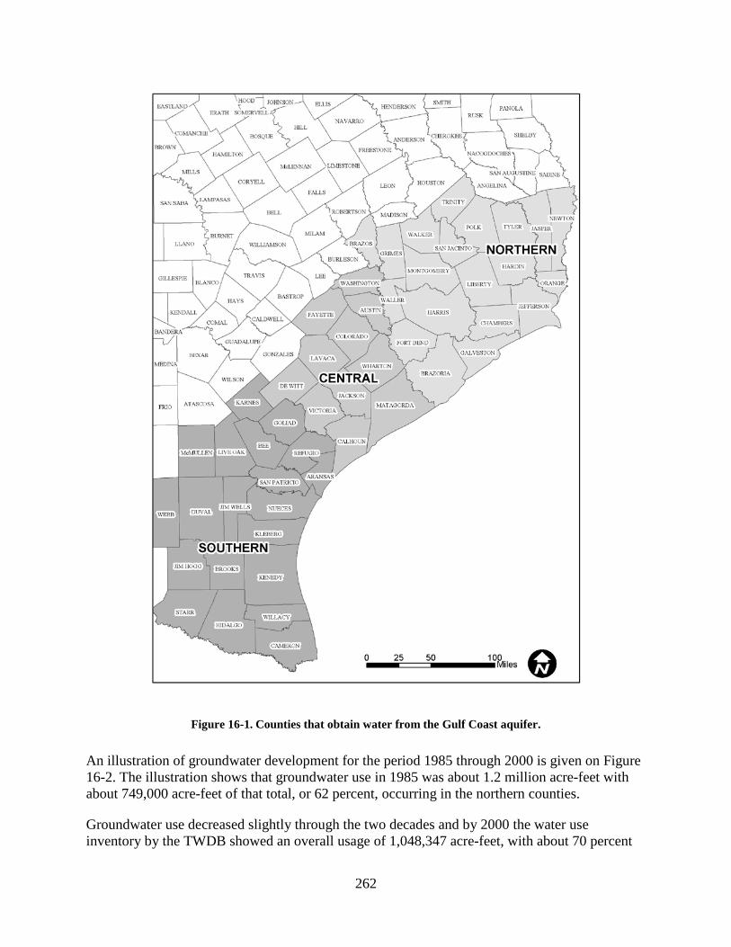
262

Figure 16-1. Counties that obtain water from the Gulf Coast aquifer.

An illustration of groundwater development for the period 1985 through 2000 is given on Figure 16-2. The illustration shows that groundwater use in 1985 was about 1.2 million acre-feet with about 749,000 acre-feet of that total, or 62 percent, occurring in the northern counties.

Groundwater use decreased slightly through the two decades and by 2000 the water use inventory by the TWDB showed an overall usage of 1,048,347 acre-feet, with about 70 percent

263

0

200,000

400,000

600,000

800,000

1,000,000

1,200,000

1,400,000

1985 1986 1987 1988 1989 1990 1991 1992 1993 1994 1995 1996 1997 1998 1999 2000

Year

Pum

ping

Am

ount

(acr

e-fe

et)

Southern Counties

Central Counties

Northern Counties

Figure 16-2. Groundwater pumpage by area from the Texas Gulf Coast aquifer for 1985 to 2000.

of that total usage occurring in the northern counties. The decrease in usage is attributable to a reduction in the quantity of water pumped for irrigation and industrial uses.

Pumpage in the southern counties ranged from about 41,000 to 67,000 acre-feet per year between 1985 and 2000. The development of groundwater in the southern counties is an essential part of the municipal supply for many of the cities and towns. Pumpage in Duval, Kleberg, Hidalgo, San Patricio, and Jim Wells counties constituted about 64 percent, or 37,890 acre-feet per year, of the total pumpage in the southern counties in 2000. The development of brackish groundwater is occurring in the Rio Grande Valley to provide water for municipal and industrial uses.

The groundwater pumpage by use category is shown on Figure 16-3. The data show that the vast majority of groundwater is pumped for municipal and irrigation uses, followed by industrial use. In 1985, approximately 47 percent of the groundwater pumped from the Gulf Coast aquifer was for municipal use and 42 percent was for irrigation. By 1999, approximately 52 percent of the groundwater pumped was for municipal use and 37 percent for irrigation. This shows the value of groundwater for municipal use and a reduction in irrigation demand due to higher fuel prices and lower relative commodity prices. A review of the data for the past 15 years shows that pumping for municipal use has fluctuated and increased gradually from 562,922 to 591,088 to 624,334 acre-feet per year in 1985, 1999, and 2000, respectively. Additional surface water supplies being routed to the Houston area probably will result in a reduction in the overall

264

0

200,000

400,000

600,000

800,000

1,000,000

1,200,000

1,400,000

1985 1986 1987 1988 1989 1990 1991 1992 1993 1994 1995 1996 1997 1998 1999 2000

Year

Pum

ping

Am

ount

(acr

e-fe

et)

Livestock

Industrial

Irrigation

Municipal

Figure 16-3. Total Gulf Coast aquifer pumpage by use for 1985 to 2000.

amount of groundwater pumped for municipal needs in that part of the state. A vast majority of the overall pumping for irrigation occurs in the central counties of the Gulf Coast aquifer region. Within these counties, irrigation constituted approximately 87 and 86 percent of the total groundwater pumped in 1985 and 1999, respectively. The groundwater withdrawal for irrigation in the central counties in 1985 and 1999 was 344,277 and 312,037 acre-feet per year, respectively. The use of groundwater for irrigation in this area is estimated to continue in the future as long as commodity prices are sufficient for continued irrigation of crops, principally rice, and as long as energy costs are not so high that they preclude the pumping of groundwater. Further reductions in groundwater withdrawals in the central counties could allow for the pumping of the water for other uses.

Houston-Galveston Area Groundwater use in the area began probably with the arrival of American Indians. As settlers came in the 1800s, shallow wells were dug, which provided water for domestic and livestock uses. Organized records of groundwater development in terms of pumping amounts began in the late 1880s. In 1890, based on records obtained from the U.S. Geological Survey, pumping was about 2.5 million gallons per day, or 2,800 acre-feet per year. An illustration of historical pumping is included as Figure 16-4 and the Houston-Galveston area is shown on Figure 16-5. As

265

0

100

200

300

400

500

60018

9018

9519

0019

0519

1019

1519

2019

2519

3019

3519

4019

4519

5019

5519

6019

6519

7019

7519

8019

8419

8519

8619

8719

8819

8919

9019

9119

9219

9319

9419

9519

9619

9719

9819

9920

0020

0120

0220

0320

04

Year

Ave

rage

Pum

ping

Am

ount

, Mill

ion

Gal

lons

Per

Day

Average Pumpage, MGDHGCSD Established Additional Distrubution

of Surface Water

Industrial and Public Supply Increases and IncreasedIrrigation

Industrial Growth and Increased Irrigation

Lake Houston SurfaceWater Supply Introduced

Figure 16-1. Historical groundwater pumpage for the Houston-Galveston area for 1890 to 2004.

the population of the area increased and industrialization was occurring, groundwater pumping reached about 90 million gallons per day, or 100,818 acre-feet per year, by 1930 and was somewhat stable through the years of the Great Depression. From 1935 to 1950, overall pumping increased dramatically from about 90 million gallons per day, or 100,818 acre-feet per year, to 300 million gallons per day, or 336,060 acre-feet per year, as industrialization occurred in the area bordering Galveston Bay, the population of the area grew dramatically, and irrigation increased in the area west of Houston. Large-capacity wells were constructed to obtain the ever-increasing amount of water.

In 1953–1954, Lake Houston was constructed and began providing a supply of surface water, which resulted in a reduction of the rate of growth of groundwater usage from 1950 to 1960. Lake Houston continues to be a major source of water for the Harris-Galveston area. Groundwater pumping peaked in the area in 1975 at just over 500 million gallons per day, or 560,100 acre-feet per year. A pumping rate of one million gallons per day for a year is equivalent to about 1,120 acre-feet of pumping per year. The pumping of large quantities of groundwater caused significant artesian head declines in the Gulf Coast aquifer that reached about 400 feet in the Houston Ship Channel area by 1975. After about 1976, pumping along the Houston Ship Channel began to decrease as the result of the introduction of surface water from the Coastal Industrial Water Authority. Overall pumping in the Houston-Galveston area decreased significantly from 1975 to 1980 and has decreased gradually from 1980 to 2004. By 2004,

266

Figure 16-5. The Houston-Galveston area.

pumping in the area was about 339 million gallons per day, or 379,747 acre-feet per year. Artesian heads have rebounded about 200 to 240 feet in the Evangeline aquifer in the Ship Channel area since 1977 as the result of reductions in pumpage in that area and in surrounding areas.

Since the establishment of the Harris-Galveston Subsidence District, groundwater usage has decreased in the continuing effort to address land surface subsidence. Surface water usage has increased and is planned to continue to increase in the future as the demand for water in Harris, Galveston, Fort Bend, and Montgomery counties is estimated to be 1,524 million gallons per day (1,707,184 acre-feet per year) and 1,841 million gallons per day (2,062,288 acre-feet per year) by 2020 and 2040, respectively, based on the Region H regional water plan completed in 2005.

267

Future Groundwater Development Groundwater supplies will continue to provide an important source of water for the Gulf Coast area. The aquifer system is capable of supplying large quantities of good quality water and has a greater potential for providing water in the area from about Victoria County northeastward toward the border with Louisiana. This same aquifer system is a prolific source of water in Louisiana.

In a high population growth area such as the Houston metropolitan region, groundwater will continue providing part of the supply with surface water from the Brazos, San Jacinto, and Trinity rivers being a larger water source. Development of groundwater resources in this region should be accomplished while being mindful of land surface subsidence constraints. The Harris-Galveston and Fort Bend subsidence districts have been instrumental in developing regulatory plans that include limits on the amount of groundwater pumping that can occur.

To the east of Harris County in Liberty, Hardin, Tyler, Jasper, and Newton counties, the Gulf Coast aquifer system is capable of providing large quantities of good quality water. In these counties groundwater usage is somewhat limited because of the lower population, availability of surface water, and generally small industrial groundwater demand. The City of Beaumont pumps groundwater in the south part of Hardin County and a paper mill in Jasper County pumps about 30,000 to 35,000 acre feet per year to supplement a supply of surface water for its paper production operations. Additional supplies of groundwater could be developed in the five counties (see Figure 16-6) if needed for local use or for transport to an area with a water need. Whether this will occur is not known, but the water resource would be a replenishable supply with abundant precipitation in the area serving as a source of recharge to the aquifer system.

Potential Groundwater Development Projects

There have been a few projects proposed that would involve development of groundwater from the Gulf Coast aquifer for use in other areas of the state or for use during times of limited surface water availability. Two projects in this category include the Lower Guadalupe Water Supply Project and the Lower Colorado River Authority-San Antonio Water System Water Project.

Lower Guadalupe Water Supply Project

This project was proposed in 2002 and included the conjunctive use of surface water and groundwater with the surface water coming from the Guadalupe River and the groundwater potentially coming from well fields in Refugio, Goliad, and Victoria counties. Objectives of the project were to develop groundwater from deeper depths of the Evangeline aquifer of the Gulf Coast aquifer system. The project would comply with the requirements of groundwater conservation district rules regarding well permitting, pumping, and the monitoring of the aquifer response to pumping. Within the last few months, the groundwater component of the project was removed. Prior to its removal, the project included the development of an average of about 14,000 acre-feet per year of groundwater to supplement surface water. There would be years when groundwater would be pumped at higher rates and years when groundwater would be pumped at lower rates to help firm up the overall yield of the project of about 80,000 to 90,000 acre-feet per year. The water was destined for use in the Bexar County area and potentially at

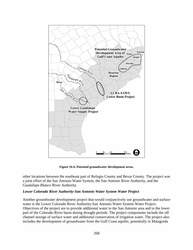
268

Figure 16-6. Potential groundwater development areas.

other locations between the southeast part of Refugio County and Bexar County. The project was a joint effort of the San Antonio Water System, the San Antonio River Authority, and the Guadalupe-Blanco River Authority.

Lower Colorado River Authority-San Antonio Water System Water Project

Another groundwater development project that would conjunctively use groundwater and surface water is the Lower Colorado River Authority-San Antonio Water System Water Project. Objectives of the project are to provide additional water to the San Antonio area and to the lower part of the Colorado River basin during drought periods. The project components include the off channel storage of surface water and additional conservation of irrigation water. The project also includes the development of groundwater from the Gulf Coast aquifer, potentially in Matagorda

269

and Wharton counties (Figure 16-6) to supply local irrigation needs during drought years so that surface water from the Colorado River can be used upstream. Potentially about 62,000 acre-feet of groundwater could be pumped during drought years for local irrigation needs. Studies are currently being performed regarding the project and, if results are favorable, water from the project could be delivered by the next decade.

Potential Brackish Groundwater Development

In addition to providing large quantities of good quality water, the Gulf Coast aquifer system also contains a substantial quantity of brackish groundwater. For this paper, brackish groundwater is defined as water containing more than 1,000 milligrams per liter total dissolved solids and less than 10,000 milligrams per liter of total dissolved solids. Areas that have been outlined as containing brackish groundwater are shown on Figure 16-7. In general, the aquifer system contains groundwater of good quality from its outcrop area to within 10 to 30 miles of the coast. In the area south of Victoria County brackish groundwater extends further inland from the coast than in the area northeast of Victoria County. Some of the same sands that contain good quality water away from the coast contain brackish water closer to the coast.

There is the potential to develop supplies of brackish groundwater and, through a total dissolved solids reduction process, normally reverse osmosis, improve the quality of the water so that it can be used for public supply, industrial, and other uses. Issues to address with this type of development include the cost of developing and treating the water and then transporting it from areas of supply to areas of use. Other issues include maintaining a reasonably stable quality of brackish water through the duration of a project, disposal of the concentrate that is a product of the reverse osmosis treatment, and potential land surface subsidence. These issues can be addressed, and the cost of addressing them affects the viability of a project.

Supplies of brackish water are being successfully developed in the Rio Grande Valley in Cameron County for the Southmost Regional Water Authority with facilities that provide about 7.5 million gallons per day, or 8,401 acre-feet per year, of desalinated water. Another desalination project was developed by the North Cameron Regional Water Authority to treat brackish groundwater and provide a supply of about 2 million gallons per day, or 2,240 acre-feet per year. These projects are examples of developing the important brackish groundwater resources that exist in the Gulf Coast aquifer system. The potential exists to develop larger desalination projects in areas along the coast and this will occur in the coming decades.

Conclusions The Gulf Coast aquifer system is an important source of water for the Gulf Coast region. The unconsolidated sediments provide a structure and medium for drilling small and large-capacity production wells that provide water for a range of uses. The aquifer system helps sustain the economic viability of the Gulf Coast region and provides the largest supplies of good quality groundwater in the area northeast of Victoria County where the aquifer system is composed of greater thicknesses of sand containing water with low levels of total dissolved solids. The aquifer system is an important source of water in the area south of Victoria County where it is still

270

Figure 16-7. Brackish groundwater areas.

capable of providing significant quantities of groundwater ranging in quality from fresh to brackish. Total pumping from the aquifer system was about 1,046,000 acre-feet in 2000.

In the future the aquifer system will continue providing large quantities of groundwater with the three main use categories being irrigation, public supply and industry. There is the potential that groundwater will be developed from the aquifer for use in other areas of the state or for transport from one part of the Gulf Coast to another. Undeveloped Gulf Coast aquifer resources occur in the east Texas area where abundant precipitation provides replenishment to the aquifer. The Gulf Coast aquifer can also provide large quantities of brackish water that can be treated to provide additional supplies for public supply, industry, and other uses. The desalination of brackish groundwater is occurring in the Rio Grande Valley and providing an additional water source to an area with an increasing water demand that relies heavily on surface water from the Rio Grande River.

271

References of Interest Epsey, Huston & Associates, Inc., 1979, Water Resource Management Program Phase I: Harris-

Galveston Coastal Subsidence District.

Fort Bend Subsidence District, 2005, 15th Annual Groundwater Report Year Ending December 31, 2004.

Harris-Galveston Coastal Subsidence District, 2005, 28th Annual Groundwater Report Year Ending December 31, 2004.

Kellogg Brown & Root/Turner Collie & Braden, Inc., 2005, Initially Prepared 2006 Regional Water Plan: Region H Water Planning Group.

Lower Colorado River Authority and San Antonio Water Supply, March 2005, LCRA-SAWS Water Project Presentation, http://www.lcra.org/docs/lswp/Project_Overview.pdf.

LBG-Guyton Associates, 2002, Brackish Groundwater Manual for Texas Regional Water Planning Groups: Texas Water Development Board.

NRS Consulting Engineers, 2005, Desalination: http://www.nrsengineers.com/desalination.htm.

Schaumburg & Polk, Inc., 2005, Initially prepared East Texas Region Plan (Region I): East Texas Regional Water Planning Group.

Weynand, P. A., 2004, San Antonio River Authority, Personal communication.

272

This page intentionally blank.

273

Chapter 17

The Challenge of Managing Groundwater in the Gulf Coast Aquifer: Recognizing and

Incorporating Divergent Value Systems Regarding Groundwater as a Resource

James A. Dodson1

Introduction People need water. A simple statement of fact, but also a good starting point for exploring how water management, particularly the management of groundwater in the Gulf Coast aquifer, is subject to the influence of personal preferences about how water should be allocated to meet these needs—preferences which are revealed in individual perspectives, or value systems, regarding groundwater as a resource. Effective groundwater management depends, in part, on understanding and accommodating the many, often divergent, value systems exhibited by those elected officials, citizens, landowners, and other stakeholders involved in the process, while still adhering to principles of sound science and state law.

This paper explores the factors involved in the development of individual value systems regarding groundwater resources, how these values are sometimes expressed, and the effect they have on the decentralized process of groundwater management in the Gulf Coast aquifer of Texas. It suggests a few elements of what could be a new framework for groundwater resource management that is designed to better enable the State to protect the resource base, promote people’s rights and interests in the use of the resource, and achieve statewide goals regarding water policy.

The content of this paper is based on the author’s experiences during a decade and a half of professional activity spent developing regional solutions to water resource management challenges in the South Texas area. While the author’s early role in this water management arena took place in the public sector, dealing primarily with surface water issues, later experiences have been in the private sector, working with landowners to develop public-private partnerships

1 President, Goliad Sands, Limited

274

that facilitate a conjunctive management approach to the more effective use of water resources. The observations and opinions contained in this paper are solely those of the author.

The Use Value of Water The human use of water ranges from the essential to the optional. Water is required to support life-sustaining biological functions, and it is used in a myriad of human endeavors that benefit the health and well being of individuals, economies, and societies. Some uses of water are more, as parents might point out to their children, in the nature of wants, rather than basic needs—but many of these less essential uses of water contribute to a quality of life that is important to the users.

Individuals inherently assign some relative value to each of these uses. These personal ideas about the role water plays in our lives, the relative value it has in various uses, who “owns” it, and the way it should be allocated among competing uses, may or may not reflect the more objectively derived management principles that have been used in traditional resource management. This is particularly evident when the decision-making process regarding groundwater management has been delegated to the local level, where stakeholders and voters, through their elected officials, can more directly express their views and preferences stemming from these personal value systems.

Where there has been little opportunity for those involved in this new, de-centralized groundwater management process to become well-versed with the legal and technical aspects of groundwater management, the value systems that seem to operate most often are those based on an individual’s subjective experience (opinions and feelings) regarding their own access to their preferred uses of water, rather than objective scientific, economic and policy analysis.

Based on observation, it appears that in many cases, fear is the underlying emotion shaping personal value systems regarding water resources—fear based on past experiences. Many people in Texas still recall the hardships experienced during the “Great Drought” of the 1950s. In the introduction to “The Time It Never Rained,” a novel about a family in West Texas during the drought of the 1950’s, writer Elmer Kelton keenly observed about Texans that:

“Each new generation tends to forget—until it confronts the sobering reality—that dryness has always been the normal condition in the western half of the state. Wet years have been the exceptions” (Kelton, 1984).

This realization, and the fear that it invokes, burns deep into the psyche of Texans who still depend on water supplies that are subject to the effects of this natural drought cycle. Although droughts affect surface water sources more immediately and directly, some aquifer systems are still vulnerable to long periods of diminished recharge and/or excessive use during droughts.

While this fear may lead to greater stakeholder involvement in the groundwater management process, it can also result in an emotionally charged atmosphere that is not particularly conducive to either building consensus on appropriate groundwater management policies or protecting the rights of stakeholders with legitimate, but minority, viewpoints. The challenge is to find ways to

275

appropriately address the subjective—even emotional—content of the value systems being expressed and to incorporate those values into an equitable, inclusive, legally defensible, and scientifically sound framework for effective groundwater resource management.

The Characteristics of Groundwater as a Resource The first task may be to demonstrate how groundwater fits in the category of a resource. The Merriam-Webster Online Dictionary defines resource as “a natural source of wealth or revenue—often used in plural” (that is, resources). Another definition of resource, found in Webster’s II New Riverside University dictionary, is: “an accessible supply that can be withdrawn from when necessary” (Soukhanov and others, 1994). Groundwater, especially groundwater in the Gulf Coast aquifer, appears to fit the definition of a resource or, more specifically, a natural resource. Implicit in the concept of a natural resource is the idea that, while existing in nature, the resource is withdrawn to meet human needs. (Although, as described later, groundwater is a natural resource that is also used to meet environmental needs.)

Setting aside for the moment the question of “to whom, if anyone, does the groundwater belong?” one might imagine an aquifer system as being somewhat analogous to a financial trust established for a diverse group of beneficiaries. In this case, the trust (the aquifer) contains an initially funded principal amount (aquifer storage) and also receives periodic additions from earnings or “cash flow” generated by processes outside the trust’s savings account (aquifer recharge). By the terms of the trust (aquifer characteristics and parameters), there is a maximum amount of principal that can to be held in the trust (total aquifer storage). Amounts in excess of this cap (discharge) may be distributed to the beneficiaries under the terms of the trust.

Professional trust officers (water resource managers) direct the trust, with input from members of a board representing the beneficiaries (those using the aquifer). The trust officers must abide by the terms of the trust (certain well-known aquifer parameters), their financial institution’s asset management policies (a local groundwater management plan), and state and federal laws governing financial institutions (that is, the Texas Water Code).

Obviously, there are many differences between managing and allocating natural resource “accounts,” like groundwater, and managing a financial trust. Exploring some of these differences may provide a few insights into the issues facing those involved in the efforts to manage groundwater resources in the Gulf Coast aquifer of Texas:

• The analogy assumes there is active management of the “trust assets,” or the groundwater in the aquifer. This is the case in those areas within the Gulf Coast aquifer in Texas where there are groundwater conservation districts (GCDs) established by the Texas Legislature to provide for “local” management of groundwater resources. The exceptions are those areas where there are no GCDs.

• Unlike financial accounts such as trusts, where performance data is readily available to facilitate decision-making, usable data on aquifer parameters and conditions may not be available except where development has already occurred and monitoring is taking place. Where development is only anticipated—the areas most in need of good information to

276

support decisions on the allocation of groundwater resources—data is scarce, at best. This often leads to decisions being made on the basis of more subjective criteria, especially criteria that reflect the value systems prevailing within the decision-making body.

• While it may be assumed that the assets of the financial trust are used to generate economic benefit, at least to certain designated groups or individuals, not all groundwater uses are for the purpose of creating pure economic benefit. Some uses are environmental in nature—supporting populations of endangered species in the springs of the Edwards aquifer, for example—and may have little directly measurable economic benefit. In the context of groundwater management and allocation, however, these uses are generally recognized as having important “non-market” values and, in some cases, have been given higher priority than other, more traditionally valued uses of groundwater.2

• In managing a financial trust, the professional trust officers often find themselves dealing with beneficiaries who have conflicting views of how the trust should be managed. While the trust officers may understand the different points of view among the beneficiaries, they don’t necessarily have the means, or an obligation, to make all the beneficiaries

2 In attempting to incorporate more of the subjective values at work among stakeholders, water planners and economists have had to address the non-market value of water resources. In fact, the non-use, or passive use, value of surface-water resources is now recognized as a legitimate economic parameter in evaluating the benefits of proposed water projects—although, because it is related to personal, aesthetic preferences, it is difficult to quantify objectively and incorporate in most economic analyses (see Hanemann, 2005 for a discussion of non-market valuation of water).

Someone once remarked—after trying unsuccessfully to generate income from a tract of rural land—that “the highest and best use of the property is just looking at it.” It may be hard to “see,” and accept, that groundwater has some inherently greater value being left in the aquifer, rather than being withdrawn for use, simply because an appreciation exists of the fact that “it’s there.” However, there are certain other values associated with non-use that may be held by some stakeholders and need to be considered: that is, the bequest value—the desire to leave it there for future generations—or, the option value—a desire to protect the resource, through current non-use, in order to have the option of potential use in the future.

Both of these two types of non-use values have, as an underlying element, some anticipated future economic benefit to be derived by actual use, albeit the use may occur at such an indeterminate time in the future that it is difficult to discount these back to a present value. In any case, the perceived value is real and appreciable to those holding these views.

Unfortunately, the allocation of groundwater under many current regulatory approaches tends to favor immediate withdrawal and actual use. For example, regulatory policies that reward use by basing permits on historic use—especially where there has been no significant prior development within an aquifer system—may penalize those who, in the past, wished to reserve the option to use groundwater in the future. Even policies based on identifying some sustainable quantity of “water available for permitting,” and then issuing permits on a “first-come, first-served” basis up to that amount, reward those who apply for and receive the “rights” to use groundwater before the permit limit is reached, and penalize those who would prefer to “bequest” that right to subsequent generations.

277

happy with their actions. The comfort the trust officers have is that, under the terms of the trust, they are responsible for making investment and distribution decisions within a strictly defined set of legal and institutional policies. In contrast, groundwater resource management in Texas has largely been delegated to local GCDs, where elected board members and the professional staff they employ are operating in an “evolving” area of state law and public policy. These local officials often must make decisions without the benefit of adequate, accurate technical information on the aquifer system they are charged with managing. As a result, they may be heavily influenced by the value systems being expressed by particular stakeholders—especially those stakeholders who can vote in or influence the next local election.

Ownership Rights in Groundwater Resources If groundwater can be considered a resource that lends itself to being used for some individual or collective benefit, then the question remains: “To whom, if anyone, does the groundwater belong?” Differing views on the ownership of groundwater, stemming from divergent value systems, create disagreement on which uses should be allowed and to whom the benefits should accrue.

It can be argued that some system of private ownership rights in water, including groundwater, is essential to encouraging investment in the infrastructure necessary to develop water supplies and make them available for use. Without such investment, whether from public or private sources, water will not be available to meet even the basic human needs. When the prospect exists of there being some means of realizing a return on investment, via, at minimum, the right to charge fees to recover the expense involved in making the water available for use, there tends to be a greater availability of water for most uses.

It is important to note that while the debate is not necessarily over the issue of ownership rights in water, there are widely diverging philosophical and legal opinions relating to whether “access to a basic water requirement is a fundamental human right implicitly and explicitly supported by international laws, declarations, and State practice” (Gleick, 1999).

Texas water law recognizes certain private ownership rights in groundwater—rights that are usually derived from ownership of the surface estate—including the right to receive whatever economic benefits accrue with the beneficial use of groundwater developed from beneath that surface estate. Historically, Texas law has provided that landowners could install wells on their property and withdraw groundwater, which they owned and could put to a recognized beneficial, non-wasteful use. Under Texas’ version of the absolute “Rule of Capture,” withdrawal of groundwater is relatively unconstrained—there is no liability involved even if a landowner’s withdrawal and use of groundwater impairs another landowner’s ability to withdraw and use groundwater from wells on his or her property.

Although there is a history of repeated rulings by the Texas Supreme Court upholding the Rule of Capture, the most recent rulings began to direct the attention of the Texas Legislature to the shortcomings of this legal doctrine as a basis for effective, equitable groundwater management (Potter, 2004). Gradually acknowledging the Texas Supreme Court’s message that the Rule of

278

Capture was no longer an effective, or equitable, method of managing groundwater usage and avoiding conflicts between landowners, the Texas Legislature has more recently authorized and encouraged the creation of groundwater conservation districts (GCDs) as the “state’s preferred method of groundwater management” (Texas Water Code, Chapter 36, Section 36.0015).

Chapter 36 of the Texas Water Code provides a detailed statement of legislative policy regarding the purpose of GCDs and establishes the legal framework for the management of groundwater under the authority of a GCD. Section 36.002 of the Texas Water Code states that:

The ownership and rights of the owners of the land and their lessees and assigns in groundwater are hereby recognized, and nothing in this code shall be construed as depriving or divesting the owners or their lessees and assigns of the ownership or rights, except as those rights may be limited or altered by rules promulgated by a district” (Texas Water Code, Section 36.002—emphasis added).

Thus, while landowners still have certain “ownership or rights” in the groundwater resources associated with the surface estate, the reality is that, where GCDs exist and have adopted rules regulating groundwater withdrawals, there are significant constraints on a landowner’s ability to fully exercise his or her “ownership or rights.”

Ideally, such constraints are based on a legitimate effort to protect, and quantify, each landowner’s respective rights to withdraw and use some amount of groundwater that does not interfere with the similar right of another landowner. If crafted properly and equitably applied, GCD management plans and rules function to provide landowners with a much greater degree of certainty regarding their rights and ownership in groundwater than what is available under the Rule of Capture.

How Groundwater Science, or the Lack Thereof, Shapes Views on Groundwater Resources People develop different perspectives on the availability and sustainability of certain resources depending on the kind of information they have access to and how that information is presented. Even though the science of hydrogeology might be able to provide ever-increasing amounts of information on the characteristics and behavior of certain aquifer systems, much of that technical information will be useless in the context of de-centralized groundwater management unless it can be communicated to the non-technical audience in simple, understandable terms.

As a scientific discipline, hydrogeology is still grappling with how to create groundwater models and other tools that are equally technically sophisticated and usable by both the stakeholders and the professionals involved in the process at the local level. Unfortunately, as the tools tend to become more complex—by necessity—the level of understanding, outside of a select group of groundwater science practitioners, diminishes in a corresponding fashion.

The situation remains that most people develop their perspectives on local groundwater resources from information that is not very well founded in science, or from information that is less than

279

ideal in its accuracy and coverage. Unfortunately, even when a good amount of scientifically valid data is available on local and regional aquifer systems, it is hard to disseminate the information in a format that is quickly and easily understood by the vast majority of the stakeholders involved in the groundwater management process.3

Misapplication of “global” information to local problems—Faced with a lack of accurate, locally relevant, and easily accessible information, people often adopt views on groundwater resources that are derived from more general information on the availability and sustainability of groundwater. Lacking locally specific information on critical aquifer characteristics such as recharge rates, quantity of water in storage, transmissivity values, and other factors which dictate an aquifer’s response to stresses, there is tendency to adopt and apply information gleaned from articles and information about conditions that may exist in other, perhaps completely different, aquifer systems. Unfortunately, news articles and other information readily available to the general public tend to focus on the problems of water scarcity and conflicts over limited water supplies—problems that may not exist in the local area.

Misinterpretation of limited data on groundwater resources—Even where there is an attempt by stakeholders to acquire and interpret technical data on local groundwater conditions, the limited amounts of data that are available, or mistakes in the way the data is analyzed, may lead to erroneous conclusions. An example might be where only a short period of record is available for measured water levels. Aquifer systems with significant storage tend to operate as temporal buffers of short-term processes that affect water levels. Where a few years of monitoring data may reveal some decreasing trend in water levels, without a long period of record, there may be no way to determine if that trend is a response to recent pumping stresses, or just a part of the normal, longer-term cycle of fluctuations in water levels. If a longer period of record were available, it might reveal that there were prior periods of both increases and decreases in water levels even during “pre-development” conditions.

Another common misinterpretation of limited hydrogeologic data is failing to consider and account for the effects of other stresses besides groundwater pumping on water levels in aquifers. In some areas overlying the Gulf Coast aquifer there has been a succession of changes in land use and vegetative cover. Changes such as an increase in impermeable cover due to urbanization or an increase in the amount of brush coverage affect the net recharge rates.4

3 The one major advance that has created some hope of bridging this communication gap is the use of computer-generated graphical displays of groundwater resources. These amazingly good visual representations of aquifer structure, characteristics, and response can be particularly effective in getting some broad base understanding of the hydrogeologic processes at work in a particular aquifer system. Unfortunately, computer-generated graphics are only as good as the information on which they are based, and data scarcity remains a seriously limiting factor in their development and deployment.

4 Mesquite, huisache, and some other invasive brush are in a category of plants called “phreatophytes”—a deep-rooted plant that obtains water from the water table. The origin of the word is Greek: phrear or phreat, meaning “well” or “spring.” It may help to picture a pasture infested with mesquite as being covered with thousands of “little

280

In some areas, where there has been little groundwater development, these factors may be more important determinants of water levels than pumping stresses. However, because precipitation and pumping data may be easier to obtain and correlate with whatever data is available on water levels, changes in water levels are sometimes associated only with variations in rainfall and/or pumping.

A Clash of Values Although Chapter 36 of the Texas Water Code sets out the broader policy goals and the legal framework for groundwater management in Texas, GCDs operate in a climate where certain value systems give rise to strongly held views that may not correspond to either the reality of the hydrogeologic conditions or existing state law on the ownership, management, and allocation of groundwater. GCDs are local governmental bodies controlled by board members chosen in local elections—elections where non-resident landowners and other legitimate stakeholders may have no voice.

This situation sets the stage for a conflict between those concerned with the business of realizing the broader state water policy goals and those concerned simply with “local control” of groundwater resources. Most often this is manifested in the area of permits for projects that are proposed to develop and “export” groundwater out of a GCD’s jurisdictional area. Since the majority of such proposed projects would involve a transfer of groundwater from rural areas to urban areas, the resulting conflict over the permits for these projects is often portrayed as a rural vs. urban “clash of values” (Kaiser, 1994).

While this may be true in some broad sense, explaining conflicts over groundwater projects like these as simply a fight between rural and urban interests ignores the fact that the permits for groundwater withdrawals are being sought by, or on behalf of, landowners in the GCD. If there were no landowners interested in exercising their rights and ownership in groundwater for the purpose of providing water for these types of projects, then there would not be a venue within which the broader rural vs. urban argument might arise.

The source of the current conflict over these proposed projects, then, would appear to originate in a clash between the value systems of the various “local” stakeholders—between the resident landowners and non-resident landowners, between large landowners and small landowners, between the “environmental community” and the “development community,” or between any of the many other categories of stakeholders having divergent interests and views on how and where groundwater resources should be used.

pumping wells” extracting stored water out of the ground and discharging it, as water vapor, through their leaves and into the atmosphere (http://www.answers.com/phreatophytes&r=67).

281

Managing Groundwater Resources—Responding to Need or Responding to Fear Under the Rule of Capture, groundwater in Texas, or at least a large part of the state, was virtually “unmanageable.” But where groundwater use was largely a matter of widely dispersed agricultural, domestic, and livestock wells, there was not a pressing need to establish a new regulatory scheme to replace the Rule of Capture.

The exceptions were aquifer systems with specifically identified problems resulting from excessive withdrawals—areas in need of groundwater management. Some special districts have been established and given authority by the Texas Legislature to address these real problems (for example, the GCDs in the Texas Panhandle over the Ogallala aquifer, the Harris-Galveston Subsidence District; and the Edwards Aquifer Authority). In these instances, the problems were well known to landowners and stakeholders within these districts, and the nature and extent of the regulatory authority provided to address the problems was clearly defined in the enabling legislation and subsequent district rules.

Chapter 35 of the Texas Water Code allows the state to designate Priority Groundwater Management Areas (also known as PGMAs) where certain problems exist and groundwater management is a high priority. The Legislature has provided that the state may create GCDs in these PGMAs, with or without local initiative, to address these problems (see Texas Water Code, Chapter 35, Sections 35.007–35.013).

More recently, however, many local GCDs have been established on the initiative of local interests because of a general concern that, lacking local control, some outside entity—usually the “water marketers” or big cities—could over-pump and “export” the groundwater in the area. It is an understandable reaction, based in the fear that a traditional way of life might be threatened by some new, large use of the groundwater resources in an area. However, it can create unrealistically high expectations about the role and the effectiveness of the resulting GCD in addressing these concerns.

Many voters, when considering the confirmation of a proposed GCD, do not realize either how little, or how much, authority is truly being granted by the state to affect “local control.” Some of the confusion may be due to a lack of familiarity with the provisions of Chapter 36 of the Texas Water Code, which governs most GCDs. Even among the legal community there is a wide range of opinion regarding the authority state law grants to these districts to carry out their mission of managing groundwater resources.

State law, however, is relatively clear that GCDs must treat all applications for pumping permits on an equitable basis, including applications for wells that would export water. GCDs have no authority to deny permits for these projects simply because they may be unpopular. As a result, GCDs often have difficulty in fulfilling some of the local expectations that gave rise to their creation.

282

A New Framework is Necessary Each of the divergent viewpoints evident among stakeholders probably has some basis in legitimate interests or concerns, but the result is that there are many different “horses” pulling the “water wagons” around Texas. It is unlikely that the Texas Legislature, having decided to de-centralize groundwater management and empower GCDs with some degree of local control over groundwater resources, will be able to herd all the horses into one corral. The challenge, and perhaps the key to success, is getting all the horses to realize the benefits of pulling their wagons in the same direction.

The goal is an effective and inclusive groundwater management process that recognizes and respects the diversity of stakeholder value systems regarding groundwater resources but also has a foundation on sound scientific principles and established state laws that govern groundwater management in Texas. Such a policy and management framework should:

• recognize and protect landowners’ rights and ownership in groundwater resources and promote the role landowners can play in facilitating the sustainable, conjunctive management of water resources;

• minimize, as far as possible, well interference so that each and every landowner can fully exercise their respective right to develop their available groundwater resources and put those resources to a beneficial use of their choice;

• recognize and help realize both the broader state water management goals and the desires of local landowners in utilizing groundwater on a sustainable basis;

• incorporate and honor uses with “non-market” values, such as environmental flows and “non-use,” including protection of the option to reserve the right of use of groundwater resources for some future generations; and

• minimize litigation over decisions made at the “local” management level.

How could this possibly be accomplished? First, it entails recognizing that there are a large number of stakeholders involved in the groundwater management process and that their level of knowledge and understanding of the hydrogeologic basis for groundwater management varies widely. The interests of all stakeholders would be well served if there were much more emphasis put on developing and implementing educational programs aimed at providing stakeholders with at least some amount of accurate, usable information about their respective aquifer systems. While there is a requirement that this be included in the approved management plan for a GCD, it may simply be beyond the ability of many local GCDs to fund and execute this task. It may be a more appropriate role for a state resource agency, like the Texas Water Development Board (TWDB), to develop and disseminate these basic educational resources. In fact, where good data exists in the Groundwater Availability Models (GAMs) developed by TWDB, it may not involve too much effort to take some of the graphical representations of aquifer system properties and use them to prepare regionally specific educational materials.

The state has already established what may be an appropriate venue for these efforts. The 79th Texas Legislature passed HB 1763, which requires local GCDs to engage in a joint planning and

283

coordination process aimed at establishing, by consensus, the “desired future conditions for the relevant aquifers in the management area.” (In this case, the “management area” for each aquifer system is a specifically delineated “Groundwater Management Area,” or GMA. GMAs were previously defined by TWDB in a rulemaking process responding to a legislative mandate contained in SB2, enacted by the 77th Texas Legislature (see SB2, Sections 2.21, 2.22, & 2.48).

Local groundwater management efforts do not operate in a vacuum. There needs to be greater effort made to communicate the importance of the broader policy goals that the Legislature has established for local groundwater management efforts and to highlight the benefits for all Texans.

It appears that the over-arching state policy with respect to groundwater management is to continue to recognize private property rights in groundwater, but to subject those rights to some limitations—based on locally specific groundwater conditions—so as to prevent well interference, waste, subsidence, and other manifestations of overuse of locally, or regionally, available groundwater resources (see Section 36.1071 of the Texas Water Code pertaining to those management goals required to be included in a GCD’s management plan).

State law also appears to recognize that groundwater resources should be available for development and use as part of the larger need to assure a long-term, dependable, affordable supply of water for regions across the state. These statewide policy goals need to be more clearly and effectively communicated to local stakeholders so they can put their individual interests and value systems in perspective with the goal of providing for the broader interests and good of the state as a whole.

One way to encourage the internalization and adoption of the statewide policy goals is to provide incentives for local GCDs and stakeholders to participate in the process of groundwater management on a more regional basis. While the state, under the provisions of HB1763, appears to be heading in the direction of requiring more regional coordination among GCDs on certain basic issues, like identifying the “desired future condition” of an aquifer or portion of an aquifer, and using this information to determine the amount of “water available for permitting,” there still remains the need to steer the de-centralized management process in more of a uniform direction.

Some stakeholders may have less fear about certain uses of groundwater if they can be assured that those uses generate identifiable benefits for the local area, in addition to achieving the goals of the landowner(s) involved and the broader goals of statewide water policy. This is where local incentives come into play. One example of an incentive may be to change state law so as to allow GCDs to use the revenues generated by export fees towards efforts designed to meet local economic development needs, rather than only for purposes of supporting the GCD’s operating budget.

A Final Thought In almost every gathering on the subject of water resources, someone will trot out the line “Whiskey is for drinking and water is for fighting.” It is always attributed to Mark Twain,

284

although one researcher scoured everything Mark Twain wrote and couldn’t find it in print. However, it certainly sounds like something Mark Twain might have said.

The truth may be that, while whiskey has probably started more fights than water, whiskey tends to fuel barroom brawls and riots, while water tends to ignite feuds, civil wars, and international conflicts. Disputes like these over water are usually rooted in divergent value systems that have not been properly identified or addressed before it is too late.

Perhaps a better paradigm would be that “whiskey is for drinking, and water is for sharing.” Getting to this new framework for groundwater management might start with the various groups involved sitting down, over a drink—water, or whiskey, depending on your value system.

References Answers.Com, 2005, http://www.answers.com/phreatophytes&r=67 (accessed November 1,

2005).

Gleick, P., 1999, The human right to water: Water Policy, v. 1, no. 5, p. 487–503.

Hanemann, M., 2005, The economic conception of water: CUDARE Working Papers, Paper 105, Department of Agricultural & Resource Economics, University of California, Berkeley, 30 p.

Kaiser, R. A., 1994, Legal and institutional barriers to water marketing in Texas: Texas Water Resources Institute Technical Report No. 67, 129 p.

Kelton, E., 1984, The time it never rained: Fort Worth, Texas, Texas Christian University Press, 378 p.

Merriam-Webster Online Dictionary, 2005, http://www.m-w.com/dictionary/resource, (accessed November 1, 2005).

Potter, H. G., III, 2004, History and evolution of the right of capture, in Mullican, W. F., III, and Schwartz, S., editors, 100 Years of the Rule of Capture—From East to Groundwater Management: Texas Water Development Board Report 361, p. 1–17.

Soukhanov and others, editors, 1994, Webster’s II New Riverside University Dictionary: Boston, Massachusetts., The Houghton Mifflin Company, 1,536 p.

Texas House, 2005, House Bill 1763, Acts 2005, 79th Texas Legislature, regular session. Vernon’s Texas Session Laws, Ch. 970.

Texas Senate, 2001, Senate Bill 2, Acts 2001, 77th Texas Legislature, regular session, Vernon’s Texas Session Laws, Ch. 966.

Texas Water Code, Chapter 35, Sections 35.007–35.013.

Texas Water Code, Chapter 36, Section 36.0015.

285

Texas Water Code, Chapter 36, Section 36.002.

Texas Water Code, Chapter 36, Section 36.1071.

286

This page intentionally blank.

287

Chapter 18

Assessment of Shallow Recharge and Groundwater-Surface Water Interactions for the

LSWP Study Region, Central Texas Coast Neil Deeds1, Van Kelley, P.G.1, Steven C. Young2, and Geoffrey P. Saunders, P.G., C.G.W.P.3

Introduction The LCRA-SAWS Water Project (LSWP) represents a partnership between the Lower Colorado River Authority (LCRA) and San Antonio Water System (SAWS) with the goal of conserving and developing water for the San Antonio region and the Lower Colorado River Basin in the 21st century. This project includes the development of a groundwater model of the Chicot and Evangeline aquifers in the study region. The study region includes Colorado, Wharton, and Matagorda counties, as well as adjacent counties, including Lavaca, Jackson, Austin, Fort Bend, and Brazoria counties.

As part of the development of a conceptual groundwater model of the study region, an analysis of shallow recharge and baseflow discharge was completed. In dipping aquifers, like the Chicot and Evangeline, recharge occurs in the outcrops where the aquifers are unconfined. The groundwater system in the outcrop can often act as a classical topographically-driven recharge/discharge system, where recharge primary occurs in the areas of higher elevation, and discharge occurs in the areas of lower elevation through streams, seeps, and groundwater evapotranspiration. The recharge to the water table that discharges relatively quickly in the surficial groundwater system does not have a significant impact on the deeper, confined aquifer system. Therefore, recharge can be conceptually divided into two different types, “shallow” recharge, which discharges relatively quickly through baseflow and other surficial discharge components, and “deep” recharge, which moves into the confined system and exits, under predevelopment conditions, through cross-formational flow. This paper discusses the analysis of the shallow recharge that discharges primarily to streams through baseflow. Understanding this part of the hydrologic system allows for the development of baseflow targets for the groundwater model as well as improving the implementation of recharge in the model.

1 INTERA Incorporated 2 URS Corporation 3 Lower Colorado River Authority

288

Hydrograph Separation Analyses Hydrograph separation is a methodology whereby streamflow hydrograph data is analyzed and surface runoff is partitioned from the stream baseflow component. The basic premise is that in the streamflow hydrograph, sharp peaks represent surface runoff events, whereas the smooth, constant portion of the streamflow hydrograph represents baseflow.

Baseflow separation studies were performed on 15 stream gages in the study area that had some historical unregulated period. The code BFI (Wahl and Wahl, 1995) was used to perform the automated separation analysis. Figure 18-1 shows the subwatersheds analyzed in the study area, along with the corresponding gages. Only data from unregulated years were analyzed, based on Slade and others (2002). An attempt was made to perform an analysis on at least one gage in each subwatershed. However, unregulated gages were not available in all subwatersheds.

!.

!.

!.

!.

!.

!.

!.

!.!.!.

!.!.!.

!.

!.

Brazos S

Lavaca E

Lavaca W

Colorado - Lavaca

Colorado S

Colorado N

Brazos - Colorado E

Brazos N

San Jacinto - Brazos E

Brazos - Colorado W

Lavaca - Guadalupe

San Jacinto - Brazos W

Harris

Brazoria

Lee

LavacaWharton

Fayette

Victoria

Liberty

Colorado

Austin

JacksonMatagorda

Fort Bend

Waller

Refugio

Montgomery

Washington

Calhoun

De Witt

Bastrop

GrimesBurleson

Goliad

Galveston

Brazos

Aransas

Chambers

Gonzales

San JacintoWilliamson

8164800

8164600

81645048164503

81645008162600

8161000

8117500

8114000

8111500

8079000

8078000

8077000

81640008162500

0 10 205Miles

­StreamsCountiesModel BoundaryEvangelineChicot

Subwatersheds

Figure 18-1. Location of gages for hydrograph separation analyses.

Four of the subwatersheds shown in Figure 18-1 do not originate in the study region. These are the northern and southern portions of the Colorado and Brazos river basins. In practice, even with an upstream gage, it is difficult to determine what portion of the baseflow originates in the study area for these rivers, since the incremental addition of baseflow in the study area may be

289

small compared to the overall inflow. Also, in some subwatersheds, the results from gages representing only a portion of the overall drainage area had to be upscaled based on the ratio of the partial to overall catchment area.

The analysis of gage data was done with the understanding that the hydrographs are affected by diversions. Some estimate of the total diversions for a particular subwatershed was known, but an accurate history of the timing of the diversions was unknown. The analysis approach weighted the total diversion amount by the fraction of time that most of the streamflow is considered baseflow, thus crudely approximating the portion of the diversion that might affect the baseflow estimate.

Table 18-1 shows the long-term average annual results of the baseflow analyses. In general, baseflow estimates were in the range of one to two inches per year when averaged over the gage drainage area. Not all subwatershed results are reported, due to problems with some analyses. For example, the Colorado and Brazos subwatersheds were affected strongly by inflows from outside the region. Also, the Colorado River has the highest diversions, which also affected the results.

Table 18-1. Hydrograph separation results.

Basin Area (mi2)

Upscaled baseflow

(afy)

Diversion adjusted baseflow

(in/yr) Lavaca W 896 45,193 0.95 Lavaca E 1,424 64,286 0.85

Lavaca - Guadalupe 905 18,635 0.39 Colorado - Lavaca 1,271 106,622 1.57

Brazos - Colorado E 1,029 106,942 1.95 San Jacinto - Brazos E 1,109 140,311 2.37

mi = mile afy = acre-feet per year in/yr = inches per year

Correlation of Baseflow with Precipitation We attempted to derive a relationship between baseflow and precipitation, mostly as a surrogate to predicting shallow recharge as a function of precipitation. For each subwatershed, the annual estimates of baseflow were converted to fluxes by dividing by the catchment area and then plotted against historical annual precipitation. Equation (1) provides a relationship derived from semi-log plots, with baseflow on the log scale. The final estimated relationship for the study area was valid between approximately 20 inches per year and 60 inches per year, yielding baseflow (or minimum shallow recharge) estimates of between 0.25 and 2.0 inches per year.

log(baseflow) = 0.05(precipitation) – 2.46 (1)

where baseflow and precipitation have units of inches per year.

290

Low Flow Study Low-flow studies have traditionally been used to estimate gaining or losing conditions in a stream. These methods basically perform a flow balance between two stream control points. The net gain, or loss, of flow between the two control points is considered to be a result of stream-aquifer gain or loss, depending upon the sign. The key to this method is the assumption that surface runoff is negligible, and that is why the studies are performed at low-flow conditions. The study was performed based upon a historical analysis the first six months of water year 2000 with emphasis on the month of November 1999 which was found to have the most stable low flow conditions since 1992.

There are a significant number of tributaries, diversions, and return flows related to wastewater treatment plants (WWTPs) along the 257.8 mile river stretch. As a result, the study attempted to add and subtract these effects accordingly. Tributary inflows were estimated where not gaged. Inflows and discharge data for WWTPs were obtained from the TCEQ. In November 1999, diversions for irrigation or other uses that would provide return flows were negligible. River water pumping for industrial use, basically isolated to power plants, was minimal as estimated from LCRA records. It was determined that for the month of November 1999, tributary inflows, daily return flow, and daily diversions were insignificant compared to mainstream streamflow rates. Evapotranspiration was also found to be at least an order of magnitude below gain/loss estimates. Table 18-2 provides the November 1999 Colorado River median gain/loss estimates for the river reach between the cities of Austin and Bay City.

Table 18-2. Low flow study results.

Reach Length

(mi) Gain/loss

(afy) Gain/loss (afy/mi)

Austin-Bastrop 53.5 -4,347 -81 Bastrop-Smithville 24 42,742 799 Smithville-LaGrange 36 -15,938 -664 LaGrange-Columbus 40.9 58,680 1,630 Columbus-Wharton 68.5 7,244 177 Wharton-Bay City 34.1 70,996 1,036 159,378 mi = mile afy = acre-feet per year afy/mi = acre-feet per year per mile of river

Results and Conclusions Hydrograph separation analyses provided estimates of long-term average baseflows for several watersheds adjacent to the lower Colorado River. Hydrograph separation in the Lower Colorado River was unsuccessful due to significant inflow from outside the study area combined with large diversions in the study area. In general, the streams in the region are gaining, with an average shallow recharge return flow of one or two inches per year.

291

Annual estimates of baseflow from the hydrograph separation analyses correlated positively with annual precipitation. A semi-log relationship was derived from this correlation that can be used to vary predicted shallow recharge based on precipitation. This study also provided an estimated baseflow for the lower Colorado River through a low-flow analysis. The lower Colorado River was found to gain about 160,000 acre-feet per year (afy) over the reaches between Austin and Bay City. This is a measurement for a single point in time, and may vary somewhat from the long-term average.

In general, the study provided a good conceptual foundation for shallow recharge and discharge in the model region and also provided guidance for surface water/groundwater calibration targets for model calibration.

References Slade, R. M., Jr., Bentley, J. T., and Michaud, D., 2002, Results of stream flow gain-loss studies

in Texas, with emphasis on gains from and losses to major and minor aquifers: U.S. Geological Survey Open-File Report 02-068, 136 p.

Wahl, K. L., and Wahl, T. L., 1995, Determining the flow of Comal Springs at New Braunfels, Texas: Texas Water '95, American Society of Civil Engineers, August 16–17, 1995, San Antonio, Texas, p. 77–86.

292

This page intentionally blank.

293

Chapter 19

Low Flow Gain-Loss Study of the Colorado River in Texas

Geoffrey P. Saunders, P.G., C.G.W.P.1

Introduction Most natural rivers gain or lose water as they interact with underlying groundwater aquifers. Lower Colorado River Authority (LCRA) and San Antonio Water Systems (SAWS) are working together on a project to benefit areas served by both agencies. Low flow gains and losses are relevant to the LCRA-SAWS Water Project, because surface water availability and water quality are most sensitive to impacts during low flow conditions such as drought. This study is designed to provide information on the base flow rate of the lower Colorado River at key locations and the gain-loss of flow in reaches between those locations. After accounting for all known additions and subtractions from measured streamflow, the net gain-loss is attributed to interaction with groundwater aquifers.

Study Area The study area, located in South-central Texas, contains several major and minor aquifers designated by the Texas Water Development Board (Ashworth and Hopkins, 1995; TWDB, 2002) as shown in Figure 19-1. Some of the aquifers designated by the TWDB, such as the Carrizo-Wilcox and Gulf Coast aquifers, are subdivided on the study area map using geologic mapping of producing zones (Bureau of Economic Geology, 1974). Also shown are locations of streamflow gauging stations and reaches between these stations.

Methodology Earlier gain-loss studies were reviewed (Slade and others, 2002). In recent years since the record flood in 1991–1992, after which LCRA’s Water Management Plan has been used as a guide in regulating low flows, the driest and lowest flow period occurred during the winter of 1999–2000.

1 Lower Colorado River Authority

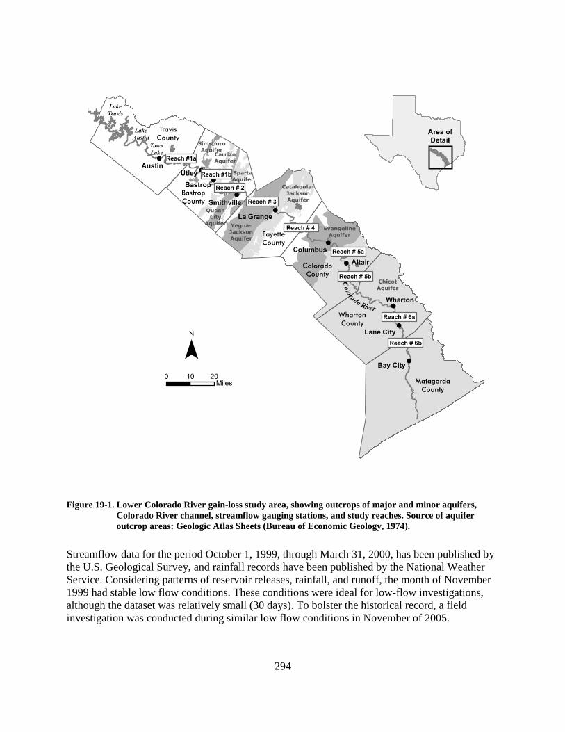
294

Figure 19-1. Lower Colorado River gain-loss study area, showing outcrops of major and minor aquifers, Colorado River channel, streamflow gauging stations, and study reaches. Source of aquifer outcrop areas: Geologic Atlas Sheets (Bureau of Economic Geology, 1974).

Streamflow data for the period October 1, 1999, through March 31, 2000, has been published by the U.S. Geological Survey, and rainfall records have been published by the National Weather Service. Considering patterns of reservoir releases, rainfall, and runoff, the month of November 1999 had stable low flow conditions. These conditions were ideal for low-flow investigations, although the dataset was relatively small (30 days). To bolster the historical record, a field investigation was conducted during similar low flow conditions in November of 2005.

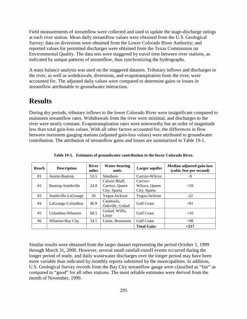
295

Field measurements of streamflow were collected and used to update the stage-discharge ratings at each river station. Mean daily streamflow values were obtained from the U.S. Geological Survey; data on diversions were obtained from the Lower Colorado River Authority; and reported values for permitted discharges were obtained from the Texas Commission on Environmental Quality. The data sets were staggered by travel time between river stations, as indicated by unique patterns of streamflow, thus synchronizing the hydrographs.

A mass balance analysis was used on the staggered datasets. Tributary inflows and discharges to the river, as well as withdrawals, diversions, and evapotranspiration from the river, were accounted for. The adjusted daily values were compared to determine gains or losses in streamflow attributable to groundwater interaction.

Results During dry periods, tributary inflows to the lower Colorado River were insignificant compared to mainstem streamflow rates. Withdrawals from the river were minimal, and discharges to the river were nearly constant. Evapotranspiration rates were noteworthy but an order of magnitude less than total gain-loss values. With all other factors accounted for, the differences in flow between mainstem gauging stations (adjusted gain-loss values) were attributed to groundwater contribution. The attribution of streamflow gains and losses are summarized in Table 19-1.

Table 19-1. Estimates of groundwater contribution to the lower Colorado River.

Reach Description River miles

Water-bearing units Larger aquifer Median adjusted gain-loss

(cubic feet per second) #1 Austin-Bastrop 53.5 Simsboro Carrizo-Wilcox -9

#2 Bastrop-Smithville 24.8 Calvert Bluff, Carrizo, Queen City, Sparta

Carrizo-Wilcox, Queen City, Sparta

+59

#3 Smithville-LaGrange 36 Yegua-Jackson Yegua-Jackson -22

#4 LaGrange-Columbus 40.9 Catahoula, Oakville, Goliad Gulf Coast +81

#5 Columbus-Wharton 68.5 Goliad, Willis, Lissie Gulf Coast +10

#6 Wharton-Bay City 34.1 Lissie, Beaumont Gulf Coast +98 Total Gain: +217

Similar results were obtained from the larger dataset representing the period October 1, 1999 through March 31, 2000. However, several small rainfall-runoff events occurred during the longer period of study, and daily wastewater discharges over the longer period may have been more variable than indicated by monthly reports submitted by the municipalities. In addition, U.S. Geological Survey records from the Bay City streamflow gauge were classified as “fair” as compared to “good” for all other stations. The most reliable estimates were derived from the month of November, 1999.

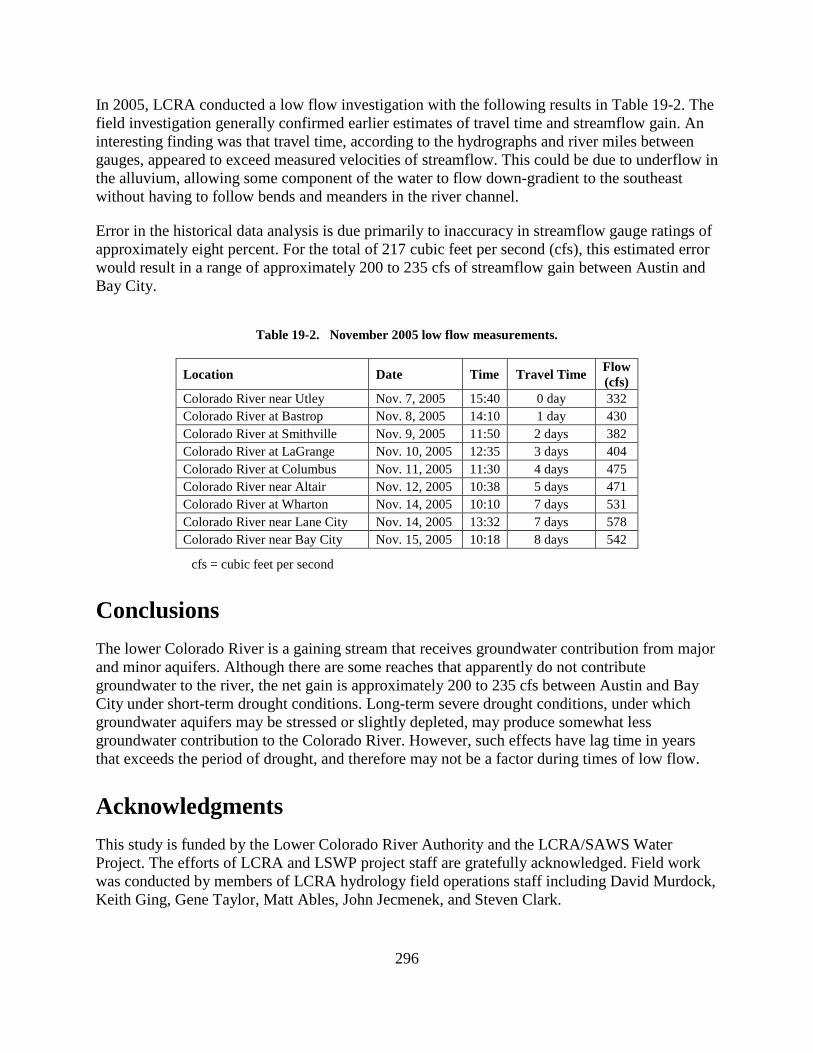
296

In 2005, LCRA conducted a low flow investigation with the following results in Table 19-2. The field investigation generally confirmed earlier estimates of travel time and streamflow gain. An interesting finding was that travel time, according to the hydrographs and river miles between gauges, appeared to exceed measured velocities of streamflow. This could be due to underflow in the alluvium, allowing some component of the water to flow down-gradient to the southeast without having to follow bends and meanders in the river channel.

Error in the historical data analysis is due primarily to inaccuracy in streamflow gauge ratings of approximately eight percent. For the total of 217 cubic feet per second (cfs), this estimated error would result in a range of approximately 200 to 235 cfs of streamflow gain between Austin and Bay City.

Table 19-2. November 2005 low flow measurements.

Location Date Time Travel Time Flow (cfs)

Colorado River near Utley Nov. 7, 2005 15:40 0 day 332 Colorado River at Bastrop Nov. 8, 2005 14:10 1 day 430 Colorado River at Smithville Nov. 9, 2005 11:50 2 days 382 Colorado River at LaGrange Nov. 10, 2005 12:35 3 days 404 Colorado River at Columbus Nov. 11, 2005 11:30 4 days 475 Colorado River near Altair Nov. 12, 2005 10:38 5 days 471 Colorado River at Wharton Nov. 14, 2005 10:10 7 days 531 Colorado River near Lane City Nov. 14, 2005 13:32 7 days 578 Colorado River near Bay City Nov. 15, 2005 10:18 8 days 542

cfs = cubic feet per second

Conclusions The lower Colorado River is a gaining stream that receives groundwater contribution from major and minor aquifers. Although there are some reaches that apparently do not contribute groundwater to the river, the net gain is approximately 200 to 235 cfs between Austin and Bay City under short-term drought conditions. Long-term severe drought conditions, under which groundwater aquifers may be stressed or slightly depleted, may produce somewhat less groundwater contribution to the Colorado River. However, such effects have lag time in years that exceeds the period of drought, and therefore may not be a factor during times of low flow.

Acknowledgments This study is funded by the Lower Colorado River Authority and the LCRA/SAWS Water Project. The efforts of LCRA and LSWP project staff are gratefully acknowledged. Field work was conducted by members of LCRA hydrology field operations staff including David Murdock, Keith Ging, Gene Taylor, Matt Ables, John Jecmenek, and Steven Clark.

297

References Ashworth, J. B., and Hopkins, J., 1995, Aquifers of Texas: Texas Water Development Board

Report 345, 69 p.

Bureau of Economic Geology, 1974, Geologic atlas of Texas, Austin sheet, Sequin sheet and Beeville–Bay City sheet: The University of Texas at Austin, 1 plate plus explanation pamphlet per sheet.

Slade, F. M., Jr., Bentley, J. T., and Michaud, A., 2002, Results of streamflow gain-loss studies in Texas, with emphasis on gains from and losses to major and minor aquifers: U.S. Geological Survey Open-File Report 02-068, published on CD-ROM.

Texas Water Development Board, 2002, Water for Texas—2002: Texas Water Development Board Document No. GP-7-1, 155 p. plus appendices.

298

This page intentionally blank.

299

Chapter 20

Groundwater Management through Groundwater Conservation Districts

Texas Alliance of Groundwater Districts

New Frontiers in Texas Water Policy In 1997, the Texas Legislature enacted Senate Bill 1, landmark legislation that instituted a bottom-up approach to state water planning through 16 regional groups representing the diversity of stakeholders. Senate Bill 1 confirmed that groundwater conservation districts “are the state’s preferred method of groundwater management” but prevented districts from prohibiting the export of groundwater. Senate Bill 1 also placed additional restrictions on exporting surface water from one river basin to another.

As a result, there is new interest in potential profit to be made from “water ranching” or groundwater marketing. Developments on this front raise the question of how to balance the private property rights of all landowners, ensuring that all benefit equitably from the groundwater resources beneath their land.

The first groundwater conservation district in Texas was established in 1951. Over the next 50 years, another 49 districts were created. Currently, 84 groundwater conservation districts have been created and confirmed by local voters and 5 districts are pending confirmation. With the new groundwater conservation districts formed in the last few years, some 89 percent of Texas’ groundwater resources are now being managed by districts (Figure 20-1). However, many of the newer districts are still in the process of developing and implementing their management plans. At the same time, most carry out their responsibilities with limited financial resources. In addition, they face real challenges in communicating their roles and responsibilities to landowners. In a November 2003 survey, members of the Texas Alliance of Groundwater Districts almost unanimously singled out “misinformation” as one of the largest problems facing new groundwater conservation districts.

In that same survey, members overwhelmingly agreed that “water marketing is one of the most serious issues facing Texas today” and that groundwater conservation districts offer a number of different management options that create a balance to the Rule of Capture. The critical issues surrounding the use and sale of groundwater in Texas demand careful and thorough attention.

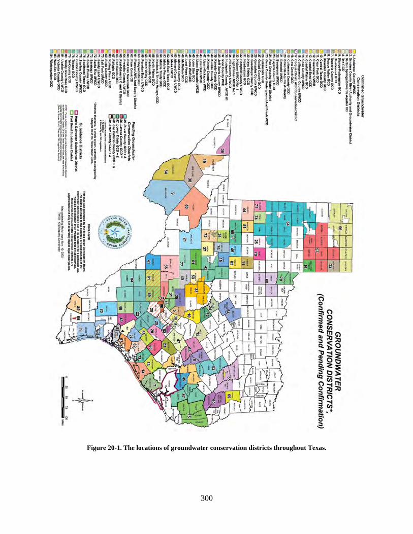
300

Figure 20-1. The locations of groundwater conservation districts throughout Texas.

301

Local Management of Local Groundwater Resources Texas is unique in the diversity of its aquifers. Recharge rates and features, depth of water tables, storage capacity, and water quality differ widely across this great state. Because of this, Texas has chosen to put management of groundwater resources in the hands of local stakeholders through groundwater conservation districts. The laws governing groundwater conservation districts are properly constructed to provide districts with flexibility to respond to the unique conditions of their particular geology and local circumstances.

Local groundwater conservation districts can set well-spacing requirements and pumping limits to ensure that pumping on one property minimizes draw-down of the water table on another. These rules can be modified as needed due to changes in population, water demand, and water table. Through these rules, districts help protect private water rights.

In areas where there is no groundwater conservation district, the “Rule of Capture” prevails. In such areas, groundwater pumping is basically unregulated. Landowners can pump as much water as they choose, without liability or regard for wells on adjacent properties.

Groundwater Conservation Districts Form Regional Alliances to Better Manage Groundwater Resources The geological formations that contain aquifers stretch beyond the political boundaries that frame individual groundwater conservation districts. A single aquifer may supply users who are separated by hundreds of miles and represented by distinct districts.

Groundwater conservation districts have recognized the real need for coordinating activities of districts that rely on the same aquifer. Many have teamed up to share staff and other resources.

In a major initiative, groundwater conservation districts are establishing alliances that help coordinate a regional approach to groundwater management strategies.

The West Texas Regional Groundwater Alliance was among the first such regional partnerships. The forerunner of the alliance was created in 1988 by Coke County Underground Water Conservation District, Glasscock County Groundwater Conservation District, Irion County Water Conservation District, and Sterling County Underground Water Conservation District. As new districts were created in adjacent counties, they too adopted the “Cooperative Agreement” providing for continuity of groundwater monitoring and protection in the region. In 1996, the agreement was redrafted, and the West Texas Regional Groundwater Alliance formed. Currently, the alliance includes 12 districts that encompass some 17,800 square miles of West Texas that overlie the Edwards-Trinity (Plateau) aquifer, one of the state’s major aquifers. Joining the four original members are Emerald Underground Water Conservation District, Hickory Underground Water Conservation District #1, Lipan-Kickapoo Water Conservation District, Lone Wolf Groundwater Conservation District, Menard County Underground Water Conservation District, Plateau Underground Water Conservation and Supply District, Santa Rita Underground Water Conservation District, and Sutton County Underground Water Conservation District.

302

The West Texas Regional Groundwater Alliance coordinates activities among member districts to promote their common objective of conserving, preserving, and providing for the beneficial use of groundwater resources. Members enjoy economies of scale by collaborating on planning, educational activities, workshops, model rules, well plugging, and legal services. Districts coordinate services, such as water quality analyses, mapping needs, computer training, and field equipment.

Other districts have formed similar regional partnerships:

• The Carrizo-Wilcox Aquifer Alliance was established in 1999 to provide for coordinated management of groundwater in South Texas. Members include Medina County Groundwater Conservation District, Evergreen Underground Water Conservation District, Bee Groundwater Conservation District, Live Oak Underground Water Conservation District, Gonzales County Underground Water Conservation District, and Wintergarden Groundwater Conservation District.

• The Hill Country Groundwater Conservation District Alliance, also formed in 1999, includes the Hays Trinity Groundwater Conservation District, Barton Springs-Edwards Aquifer Conservation District, Blanco-Pedernales Groundwater Conservation District, Hill Country Underground Water Conservation District, Cow Creek Groundwater Conservation District, Trinity Glen Rose Groundwater Conservation District, Headwaters Groundwater Conservation District, Bandera County River Authority and Groundwater District, and Medina County Groundwater Conservation District.

• The Far West Texas Alliance of Groundwater Districts, established in January 2004, encompasses Brewster County Groundwater Conservation District, Culberson County Groundwater Conservation District, Hudspeth County Underground Water Conservation District #1, Jeff Davis County Underground Water Conservation District, Middle Pecos GCD, and Presidio County Underground Water Conservation District. These districts cover two major aquifers and eight minor aquifers.

• The South Texas Regional Groundwater Alliance also was formed in early 2004. Its members include Live Oak Underground Water Conservation District, Bee Groundwater Conservation District, Goliad County Groundwater Conservation District, Evergreen Underground Water Conservation District, Refugio Groundwater Conservation District, Pecan Valley Groundwater Conservation District, and Crossroads Groundwater Conservation District.

Groundwater Conservation District Roles & Responsibilities Most groundwater conservation districts are created through legislation, usually introduced by the local state senator or representative at the request of landowners or other stockholders. Landowners can petition the Texas Commission on Environmental Quality to form a groundwater conservation district or request annexation into an existing adjacent groundwater conservation district. The Texas Commission on Environmental Quality can also create a groundwater conservation district where there is proven need for a district.

303

Most groundwater conservation districts must be confirmed by local voters. Texas law guarantees local control by requiring that all districts be managed by locally elected or appointed directors who live within district boundaries. Districts may be funded by different mechanisms, including pumping fees, administrative fees, and ad valorem taxes.

Groundwater conservation districts are required by law to develop and submit a groundwater management plan for state certification. The plan must provide for the most efficient use of local groundwater resources, control of land subsidence, and prevention of water waste. In addition, the plan must include provisions related to drought, conservation, natural resource issues, and conjunctive surface water issues.

Each district also must:

• adopt rules needed to implement the plan,

• keep records on water wells and the production and use of groundwater,

• permit and register certain wells, and

• adopt and follow administrative and financial procedures.

304

This page intentionally blank.