LIDS Report 2778 1

On Distributed Averaging Algorithms andQuantization Effects∗

Angelia Nedic†, Alex Olshevsky, Asuman Ozdaglar, and John N. Tsitsiklis‡

November 26, 2007

Abstract

We consider distributed iterative algorithms for the averaging problem over time-varying topologies. Our focus is on the convergence time of such algorithms whencomplete (unquantized) information is available, and on the degradation of perfor-mance when only quantized information is available. We study a large and naturalclass of averaging algorithms, which includes the vast majority of algorithms pro-posed to date, and provide tight polynomial bounds on their convergence time. Wethen propose and analyze distributed averaging algorithms under the additionalconstraint that agents can only store and communicate quantized information.We show that these algorithms converge to the average of the initial values of theagents within some error. We establish bounds on the error and tight bounds onthe convergence time, as a function of the number of quantization levels.

∗This research was partially supported by the National Science Foundation under grants ECCS-0701623 and DMI-0545910, and by DARPA ITMANET program

†A. Nedic is with the Industrial and Enterprise Systems Engineering Department, University ofIllinois at Urbana-Champaign, Urbana IL 61801 (e-mail:angelia@uiuc.edu)

‡A. Olshevsky, A. Ozdaglar, and J. N. Tsitsiklis are with the Laboratory for Information and De-cision Systems, Electrical Engineering and Computer Science Department, Massachusetts Institute ofTechnology, Cambridge MA, 02139 (e-mails: alex o@mit.edu, asuman@mit.edu, jnt@mit.edu)

1 Introduction

There has been much recent interest in distributed control and coordination of networksconsisting of multiple, potentially mobile, agents. This is motivated mainly by theemergence of large scale networks, characterized by the lack of centralized access to in-formation and time-varying connectivity. Control and optimization algorithms deployedin such networks should be completely distributed, relying only on local observationsand information, and robust against unexpected changes in topology such as link ornode failures.

A canonical problem in distributed control is the consensus problem. The objective inthe consensus problem is to develop distributed algorithms that can be used by a groupof agents in order to reach agreement (consensus) on a common decision (representedby a scalar or a vector value). The agents start with some different initial decisionsand communicate them locally under some constraints on connectivity and inter-agentinformation exchange. The consensus problem arises in a number of applications includ-ing coordination of UAVs (e.g., aligning the agents’ directions of motion), informationprocessing in sensor networks, and distributed optimization (e.g., agreeing on the esti-mates of some unknown parameters). The averaging problem is a special case in whichthe goal is to compute the exact average of the initial values of the agents. A naturaland widely studied consensus algorithm, proposed and analyzed by Tsitsiklis [17] andTsitsiklis et al. [18], involves, at each time step, every agent taking a weighted averageof its own value with values received from some of the other agents. Similar algorithmshave been studied in the load-balancing literature (see for example [7]). Motivated byobserved group behavior in biological and dynamical systems, the recent literature incooperative control has studied similar algorithms and proved convergence results undervarious assumptions on agent connectivity and information exchange (see [19], [14], [16],[13], [12]).

In this paper, our goal is to provide tight bounds on the convergence time (defined asthe number of iterations required to reduce a suitable Lyapunov function by a constantfactor) of a general class of consensus algorithms, as a function of the number n ofagents. We focus on algorithms that are designed to solve the averaging problem. Weconsider both problems where agents have access to exact values and problems whereagents only have access to quantized values of the other agents. Our contributions canbe summarized as follows.

In the first part of the paper, we consider the case where agents can exchange andstore continuous values, which is a widely adopted assumption in the previous literature.We consider a large class of averaging algorithms defined by the condition that theweight matrix is a possibly nonsymmetric, doubly stochastic matrix. For this class ofalgorithms, we prove that the convergence time is O(n2/η), where n is the number ofagents and η is a lower bound on the nonzero weights used in the algorithm. To thebest of our knowledge, this is the best polynomial-time bound on the convergence time ofsuch algorithms. We also show that this bound is tight. Since in the worst case, we mayhave η = Θ(1/n), this result implies an O(n3) bound on convergence time. In Section4, we present a distributed algorithm that selects the weights dynamically, using three-hop neighborhood information. Under the assumption that the underlying connectivity

2

graph at each iteration is undirected, we establish an improved O(n2) upper bound onconvergence time. This matches the best currently available convergence time guaranteefor the much simpler case of static connectivity graphs.

In the second part of the paper, we impose the additional constraint that agents canonly store and transmit quantized values. This model provides a good approximationfor communication networks that are subject to communication bandwidth or storageconstraints. We focus on a particular quantization rule, which rounds down the values tothe nearest quantization level. We propose a distributed algorithm that uses quantizedvalues and, using a slightly different Lyapunov function, we show that the algorithmguarantees the convergence of the values of the agents to a common value. In particular,we prove that all agents have the same value after O((n2/η) log(nQ)) time steps, whereQ is the number of quantization levels per unit value. Due to the rounding-down featureof the quantizer, this algorithm does not preserve the average of the values at eachiteration. However, we provide bounds on the error between the final consensus valueand the initial average, as a function of the number Q of available quantization levels.In particular, we show that the error goes to 0 at a rate of (logQ)/Q, as the number Qof quantization levels increases to infinity.

Other than the papers cited above, our work is also related to [10] and [5, 4], whichstudied the effects of quantization on the performance of averaging algorithms. In [10],Kashyap et al. proposed randomized gossip-type quantized averaging algorithms underthe assumption that each agent value is an integer. They showed that these algorithmspreserve the average of the values at each iteration and converge to approximate consen-sus. They also provided bounds on the convergence time of these algorithms for specificstatic topologies (fully connected and linear networks). In the recent work [4], Carli et al.proposed a distributed algorithm that uses quantized values and preserves the average ateach iteration. They showed favorable convergence properties using simulations on somestatic topologies, and provided performance bounds for the limit points of the generatediterates. Our results on quantized averaging algorithms differ from these works in thatwe study a more general case of time-varying topologies, and provide tight polynomialbounds on both the convergence time and the discrepancy from the initial average, interms of the number of quantization levels.

The paper is organized as follows. In Section 2, we introduce a general class ofaveraging algorithms, and present our assumptions on the algorithm parameters and onthe information exchange among the agents. In Section 3, we present our main resulton the convergence time of the averaging algorithms under consideration. In Section 4,we present a distributed averaging algorithm for the case of undirected graphs, whichpicks the weights dynamically, resulting in an improved bound on the convergence time.In Section 5, we propose and analyze a quantized version of the averaging algorithm. Inparticular, we establish bounds on the convergence time of the iterates, and on the errorbetween the final value and the average of the initial values of the agents. Finally, wegive our concluding remarks in Section 6.

3

2 A Class of Averaging Algorithms

We consider a set N = {1, 2, . . . , n} of agents, which will henceforth be referred to as“nodes.” Each node i starts with a scalar value xi(0). At each nonnegative integer timek, node i receives from some of the other nodes j a message with the value of xj(k), andupdates its value according to:

xi(k + 1) =n∑

j=1

aij(k)xj(k), (1)

where the aij(k) are nonnegative weights with the property that aij(k) > 0 only if nodei receives information from node j at time k. We use the notation A(k) to denotethe weight matrix [aij(k)]i,j=1,...,n. Given a matrix A, we use E(A) to denote the set ofdirected edges (j, i), including self-edges (i, i), such that aij > 0. At each time k, thenodes’ connectivity can be represented by the directed graph G(k) = (N, E(A(k))).

Our goal is to study the convergence of the iterates xi(k) to the average of the initialvalues, (1/n)

∑ni=1 xi(0), as k approaches infinity. In order to establish such convergence,

we impose some assumptions on the weights aij(k) and the graph sequence G(k).

Assumption 1 For each k, the weight matrix A(k) is a doubly stochastic matrix withpositive diagonal. Additionally, there exists a constant η > 0 such that if aij(k) > 0,then aij(k) ≥ η.

The double stochasticity assumption on the weight matrix guarantees that the av-erage of the node values remains the same at each iteration (cf. the proof of Lemma1 below). The second part of this assumption states that each node gives significantweight to its values and to the values of its neighbors at each time k.

Our next assumption ensures that the graph sequence G(k) is sufficiently connectedfor the nodes to repeatedly influence each other’s values.

Assumption 2 There exists an integer B ≥ 1 such that the directed graph(N, E(A(kB))

⋃E(A(kB + 1))

⋃· · ·

⋃E(A((k + 1)B − 1))

)is strongly connected for all nonnegative integers k.

Any algorithm of the form given in Eq. (1) with the sequence of weights aij(k)satisfying Assumptions 1 and 2 solves the averaging problem. This is formalized in thefollowing theorem.

Theorem 1 Let Assumptions 1 and 2 hold. Let {x(k)} be generated by the algorithm(1). Then, for all i, we have

limk→∞

xi(k) =1

n

n∑j=1

xj(0).

4

This theorem is a minor modification of known results in [17, 18, 9, 3], where theconvergence of each xi(k) to the same value is established under weaker versions ofAssumptions 1 and 2. The fact that the limit is the average of the entries of the vectorx(0) follows from the fact that multiplication of a vector by a doubly stochastic matrixpreserves the average of the vector’s components.

Recent research has focused on methods of choosing weights aij(k) that satisfy As-sumptions 1 and 2, and minimize the convergence time of the resulting averaging algo-rithm (see [20] for the case of static graphs, see [14] and [2] for the case of symmetricweights, i.e., weights satisfying aij(k) = aji(k), and also see [6]). For static graphs, somerecent results on optimal time-invariant algorithms may be found in [15].

3 Convergence time

In this section, we give an analysis of the convergence time of averaging algorithmsof the form (1). Our goal is to obtain tight estimates of the convergence time, underAssumptions 1 and 2.

As a convergence measure, we use the “sample variance” of a vector x ∈ Rn, defined

as

V (x) =n∑

i=1

(xi − x)2,

where x is the average of the entries of x:

x =1

n

n∑i=1

xi.

Let x(k) denote the vector of node values at time k [i.e., the vector of iteratesgenerated by algorithm (1) at time k]. We are interested in providing an upper boundon the number of iterations it takes for the “sample variance” V (x(k)) to decrease to asmall fraction of its initial value V (x(0)). We first establish some technical preliminariesthat will be key in the subsequent analysis. In particular, in the next subsection, weexplore several implications of the double stochasticity assumption on the weight matrixA(k).

3.1 Preliminaries on Doubly Stochastic Matrices

We begin by analyzing how the sample variance V (x) changes when the vector x ismultiplied by a doubly stochastic matrix A. The next lemma shows that V (Ax) ≤ V (x).Thus, under Assumption 1, the sample variance V (x(k)) is nonincreasing in k, andV (x(k)) can be used as a Lyapunov function.

Lemma 1 Let A be a doubly stochastic matrix. Then,1 for all x ∈ Rn,

V (Ax) = V (x)−∑i<j

wij(xi − xj)2,

1In the sequel, the notation∑

i<j will be used to denote the double sum∑n

j=1

∑j−1i=1 .

5

where wij is the (i, j)-th entry of the matrix AT A.

Proof. Let 1 denote the vector in Rn with all entries equal to 1. The double stochasticity

of A impliesA1 = 1, 1T A = 1T .

Note that multiplication by a doubly stochastic matrix A preserves the average of theentries of a vector, i.e., for any x ∈ R

n, there holds

Ax =1

n1T Ax =

1

n1T x = x.

We now write the quadratic form V (x)− V (Ax) explicitly, as follows:

V (x)− V (Ax) = (x− x1)T (x− x1)− (Ax−Ax1)T (Ax− Ax1)

= (x− x1)T (x− x1)− (Ax− xA1)T (Ax− xA1)

= (x− x1)T (I −AT A)(x− x1). (2)

Let wij be the (i, j)-th entry of AT A. Note that AT A is symmetric and stochastic,so that wij = wji and wii = 1−∑

j �=i wij. Then, it can be verified that

AT A = I −∑i<j

wij(ei − ej)(ei − ej)T , (3)

where ei is a unit vector with the i-th entry equal to 1, and all other entries equal to 0(see also [21] where a similar decomposition was used).

By combining Eqs. (2) and (3), we obtain

V (x)− V (Ax) = (x− x1)T(∑

i<j

wij(ei − ej)(ei − ej)T)(x− x1)

=∑i<j

wij(xi − xj)2.

Note that the entries wij(k) of A(k)T A(k) are nonnegative, because the weight matrixA(k) has nonnegative entries. In view of this, Lemma 1 implies that

V (x(k + 1)) ≤ V (x(k)) for all k.

Moreover, the amount of variance decrease is given by

V (x(k))− V (x(k + 1)) =∑i<j

wij(k)(xi(k)− xj(k))2.

We will use this result to provide a lower bound on the amount of decrease of the samplevariance V (x(k)) in between iterations.

6

Since every positive entry of A(k) is at least η, it follows that every positive entry ofA(k)T A(k) is at least η2. Therefore, it is immediate that

if wij(k) > 0, then wij(k) ≥ η2.

In our next lemma, we establish a stronger lower bound. In particular, we find it usefulto focus not on an individual wij, but rather on all wij associated with edges (i, j) thatcross a particular cut in the graph (N, E(ATA)). For such groups of wij , we prove alower bound which is linear in η, as seen in the following.

Lemma 2 Let A be a stochastic matrix with positive diagonal, and assume that itssmallest positive entry is at least η. Also, let (S−, S+) be a partition of the set N ={1, . . . , n} into two disjoint sets. If ∑

i∈S−, j∈S+

wij > 0,

then ∑i∈S−, j∈S+

wij ≥ η

2.

Proof. Let∑

i∈S−, j∈S+ wij > 0. From the definition of the weights wij, we havewij =

∑k akiakj, which shows that there exist i ∈ S−, j ∈ S+, and some k such that

aki > 0 and akj > 0. For either case where k belongs to S− or S+, we see that thereexists an edge in the set E(A) that crosses the cut (S−, S+). Let (i∗, j∗) be such an edge.Without loss of generality, we assume that i∗ ∈ S− and j∗ ∈ S+.

We define

C+j∗ =

∑i∈S+

aj∗i,

C−j∗ =

∑i∈S−

aj∗i.

See Figure 1(a) for an illustration. Since A is a stochastic matrix, we have

C−j∗ + C+

j∗ = 1,

implying that at least one of the following is true:

Case (a): C−j∗ ≥

1

2,

Case (b): C+j∗ ≥

1

2.

We consider these two cases separately. In both cases, we focus on a subset of the edgesand we use the fact that the elements wij correspond to paths of length 2, with one stepin E(A) and another in E(AT ).

7

i

j

Cj

C+jS+

S

i

j

S+

S

j

S+

i

S

Figure 1: (a) Intuitively, C+j∗ measures how much weight j∗ assigns to nodes in S+ (including

itself), and C−j∗ measures how much weight j∗ assigns to nodes in S−. Note that the edge

(j∗, j∗) is also present, but not shown. (b) For the case where C−j∗ ≥ 1/2, we only focus on

two-hop paths between j∗ and elements i ∈ S− obtained by taking (i, j∗) as the first step andthe self-edge (j∗, j∗) as the second step. (c) For the case where C+

j∗ ≥ 1/2, we only focus ontwo-hop paths between i∗ and elements j ∈ S+ obtained by taking (i∗, j∗) as the first step inE(A) and (j∗, j) as the second step in E(AT ).

Case (a): C−j∗ ≥ 1/2.

We focus on those wij with i ∈ S− and j = j∗. Indeed, since all wij are nonnegative, wehave ∑

i∈S−, j∈S+

wij ≥∑i∈S−

wij∗. (4)

For each element in the sum on the right-hand side, we have

wij∗ =n∑

k=1

aki akj∗ ≥ aj∗i aj∗j∗ ≥ aj∗i η,

where the inequalities follow from the facts that A has nonnegative entries, its diagonalentries are positive, and its positive entries are at least η. Consequently,∑

i∈S−wij∗ ≥ η

∑i∈S−

aj∗i = η C−j∗ . (5)

Combining Eqs. (4) and (5), and recalling the assumption C−j∗ ≥ 1/2, the result follows.

An illustration of this argument can be found in Figure 1(b).Case (b): C+

j∗ ≥ 1/2.We focus on those wij with i = i∗ and j ∈ S+. We have∑

i∈S−, j∈S+

wij ≥∑j∈S+

wi∗j , (6)

since all wij are nonnegative. For each element in the sum on the right-hand side, wehave

wi∗j =

n∑k=1

aki∗ akj ≥ aj∗i∗ aj∗j ≥ η aj∗j ,

8

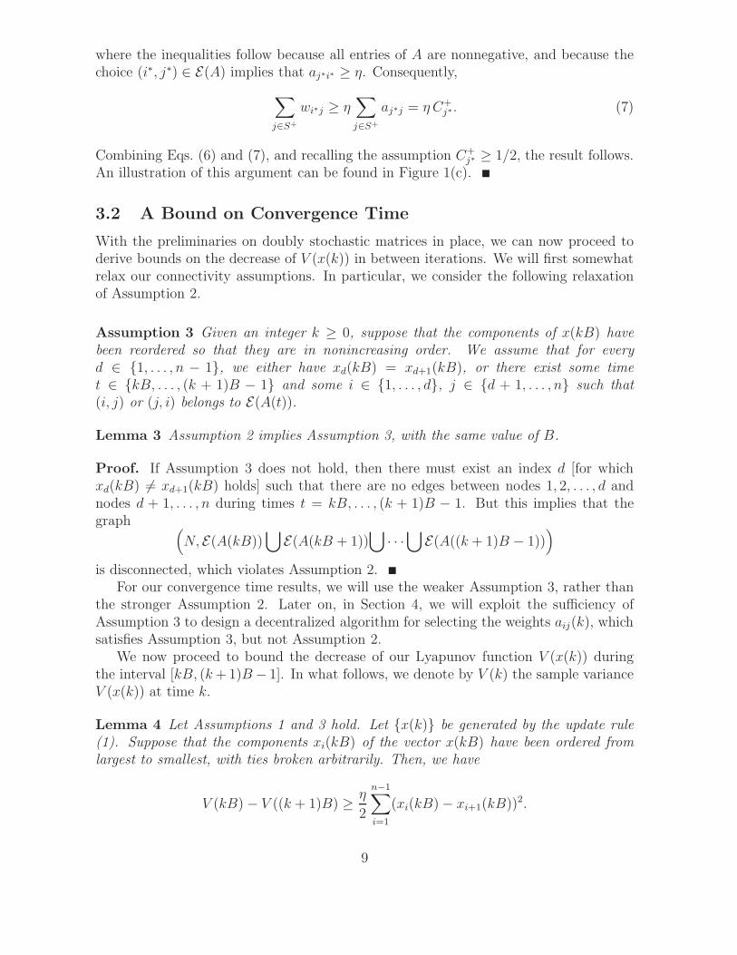
where the inequalities follow because all entries of A are nonnegative, and because thechoice (i∗, j∗) ∈ E(A) implies that aj∗i∗ ≥ η. Consequently,∑

j∈S+

wi∗j ≥ η∑j∈S+

aj∗j = η C+j∗. (7)

Combining Eqs. (6) and (7), and recalling the assumption C+j∗ ≥ 1/2, the result follows.

An illustration of this argument can be found in Figure 1(c).

3.2 A Bound on Convergence Time

With the preliminaries on doubly stochastic matrices in place, we can now proceed toderive bounds on the decrease of V (x(k)) in between iterations. We will first somewhatrelax our connectivity assumptions. In particular, we consider the following relaxationof Assumption 2.

Assumption 3 Given an integer k ≥ 0, suppose that the components of x(kB) havebeen reordered so that they are in nonincreasing order. We assume that for everyd ∈ {1, . . . , n − 1}, we either have xd(kB) = xd+1(kB), or there exist some timet ∈ {kB, . . . , (k + 1)B − 1} and some i ∈ {1, . . . , d}, j ∈ {d + 1, . . . , n} such that(i, j) or (j, i) belongs to E(A(t)).

Lemma 3 Assumption 2 implies Assumption 3, with the same value of B.

Proof. If Assumption 3 does not hold, then there must exist an index d [for whichxd(kB) �= xd+1(kB) holds] such that there are no edges between nodes 1, 2, . . . , d andnodes d + 1, . . . , n during times t = kB, . . . , (k + 1)B − 1. But this implies that thegraph (

N, E(A(kB))⋃E(A(kB + 1))

⋃· · ·

⋃E(A((k + 1)B − 1))

)is disconnected, which violates Assumption 2.

For our convergence time results, we will use the weaker Assumption 3, rather thanthe stronger Assumption 2. Later on, in Section 4, we will exploit the sufficiency ofAssumption 3 to design a decentralized algorithm for selecting the weights aij(k), whichsatisfies Assumption 3, but not Assumption 2.

We now proceed to bound the decrease of our Lyapunov function V (x(k)) duringthe interval [kB, (k + 1)B− 1]. In what follows, we denote by V (k) the sample varianceV (x(k)) at time k.

Lemma 4 Let Assumptions 1 and 3 hold. Let {x(k)} be generated by the update rule(1). Suppose that the components xi(kB) of the vector x(kB) have been ordered fromlargest to smallest, with ties broken arbitrarily. Then, we have

V (kB)− V ((k + 1)B) ≥ η

2

n−1∑i=1

(xi(kB)− xi+1(kB))2.

9

Proof. By Lemma 1, we have for all t,

V (t)− V (t + 1) =∑i<j

wij(t)(xi(t)− xj(t))2, (8)

where wij(t) is the (i, j)-th entry of A(t)T A(t). Summing up the variance differencesV (t)− V (t + 1) over different values of t, we obtain

V (kB)− V ((k + 1)B) =

(k+1)B−1∑t=kB

∑i<j

wij(t)(xi(t)− xj(t))2. (9)

We next introduce some notation.

(a) For all d ∈ {1, . . . , n − 1}, let td be the first time larger than or equal to kB (ifit exists) at which there is a communication between two nodes belonging to thetwo sets {1, . . . , d} and {d+1, . . . , n}, to be referred to as a communication acrossthe cut d.

(b) For all t ∈ {kB, . . . , (k + 1)B − 1}, let D(t) = {d | td = t}, i.e., D(t) consistsof “cuts” d ∈ {1, . . . , n − 1} such that time t is the first communication timelarger than or equal to kB between nodes in the sets {1, . . . , d} and {d+1, . . . , n}.Because of Assumption 3, the union of the sets D(t) includes all indices 1, . . . , n−1,except possibly for indices for which xd(kB) = xd+1(kB).

(c) For all d ∈ {1, . . . , n− 1}, let Cd = {(i, j) | i ≤ d, d + 1 ≤ j}.(d) For all t ∈ {kB, . . . , (k + 1)B − 1}, let Fij(t) = {d ∈ D(t) | (i, j) ∈ Cd}, i.e., Fij(t)

consists of all cuts d such that the edge (i, j) at time t is the first communicationacross the cut at a time larger than or equal to kB.

(e) To simplify notation, let yi = xi(kB). By assumption, we have y1 ≥ · · · ≥ yn.

We make two observations, as follows:

(1) Suppose that d ∈ D(t). Then, for some (i, j) ∈ Cd, we have either aij(t) > 0 oraji(t) > 0. In either case, we obtain wij(t) > 0. By Lemma 2, we obtain∑

(i,j)∈Cd

wij(t) ≥ η

2. (10)

(2) Fix some (i, j), with i < j, and time t ∈ {kB, . . . , (k + 1)B − 1}, and supposethat Fij(t) is nonempty. Let Fij(t) = {d1, . . . , dk}, where the dj are arranged inincreasing order. Since d1 ∈ Fij(t), we have d1 ∈ D(t) and therefore td1 = t. Bythe definition of td1 , this implies that there has been no communication between anode in {1, . . . , d1} and a node in {d1+1, . . . , n} during the time interval [kB, t−1].It follows that xi(t) ≥ yd1. By a symmetrical argument, we also have

xj(t) ≤ ydk+1. (11)

10

These relations imply that

xi(t)− xj(t) ≥ yd1 − ydk+1 =

k−1∑h=1

(ydh− ydh+1

) + (ydk− ydk+1)≥

∑d∈Fij(t)

(yd − yd+1),

where the last inequality follows because we have ydi− ydi+1

≥ ydi− ydi+1 for all

i = 1, . . . , k − 1. Since the components of y are sorted in nonincreasing order, wehave yd− yd+1 ≥ 0, for every d ∈ Fij(t). For any nonnegative numbers zi, we have

(z1 + · · ·+ zk)2 ≥ z2

1 + · · ·+ z2k ,

which implies that

(xi(t)− xj(t))2 ≥

∑d∈Fij(t)

(yd − yd+1)2. (12)

We now use these two observations to provide a lower bound on the expression on theright-hand side of Eq. (8) at time t. We use Eq. (12) and then Eq. (10), to obtain∑

i<j

wij(t)(xi(t)− xj(t))2 ≥

∑i<j

wij(t)∑

d∈Fij(t)

(yd − yd+1)2

=∑

d∈D(t)

∑(i,j)∈Cd

wij(t)(yd − yd+1)2

≥ η

2

∑d∈D(t)

(yd − yd+1)2.

We now sum both sides of the above inequality for different values of t, and use Eq. (9),to obtain

V (kB)− V ((k + 1)B) =

(k+1)B−1∑t=kB

∑i<j

wij(t)(xi(t)− xj(t))2

≥ η

2

(k+1)B−1∑t=kB

∑d∈D(t)

(yd − yd+1)2

=η

2

n−1∑d=1

(yd − yd+1)2,

where the last inequality follows from the fact that the union of the sets D(t) is onlymissing those d for which yd = yd+1.

We next establish a bound on the variance decrease that plays a key role in ourconvergence analysis.

Lemma 5 Let Assumptions 1 and 3 hold, and suppose that V (kB) > 0. Then,

V (kB)− V ((k + 1)B)

V (kB)≥ η

2n2for all k.

11

Proof. Without loss of generality, we assume that the components of x(kB) have beensorted in nonincreasing order. By Lemma 4, we have

V (kB)− V ((k + 1)B) ≥ η

2

n−1∑i=1

(xi(kB)− xi+1(kB))2.

This implies that

V (kB)− V ((k + 1)B)

V (kB)≥ η

2

∑n−1i=1 (xi(kB)− xi+1(kB))2∑n

i=1(xi(kB)− x(kB))2.

Observe that the right-hand side does not change when we add a constant to everyxi(kB). We can therefore assume, without loss of generality, that x(kB) = 0, so that

V (kB)− V ((k + 1)B)

V (kB)≥ η

2min

x1≥x2≥···≥xnPi xi=0

∑n−1i=1 (xi − xi+1)

2∑ni=1 x2

i

.

Note that the right-hand side is unchanged if we multiply each xi by the same constant.Therefore, we can assume, without loss of generality, that

∑ni=1 x2

i = 1, so that

V (kB)− V ((k + 1)B)

V (kB)≥ η

2min

x1≥x2≥···≥xnP

i xi=0,P

i x2i=1

n−1∑i=1

(xi − xi+1)2. (13)

The requirement∑

i x2i = 1 implies that the average value of x2

i is 1/n, which impliesthat there exists some j such that |xj | ≥ 1/

√n. Without loss of generality, let us suppose

that this xj is positive.2

The rest of the proof relies on a technique from [11] to provide a lower bound on theright-hand side of Eq. (13). Let

zi = xi − xi+1 for i < n, and zn = 0.

Note that zi ≥ 0 for all i andn∑

i=1

zi = x1 − xn.

Since xj ≥ 1/√

n for some j, we have that x1 ≥ 1/√

n; since∑n

i=1 xi = 0, it follows thatat least one xi is negative, and therefore xn < 0. This gives us

n∑i=1

zi ≥ 1√n

.

Combining with Eq. (13), we obtain

V (kB)− V ((k + 1)B)

V (kB)≥ η

2min

zi≥0,P

i zi≥1/√

n

n∑i=1

z2i .

2Otherwise, we can replace x with −x and subsequently reorder to maintain the property that thecomponents of x are in descending order. It can be seen that these operations do not affect the objectivevalue.

12

The minimization problem on the right-hand side is a symmetric convex optimizationproblem, and therefore has a symmetric optimal solution, namely zi = 1/n1.5 for all i.This results in an optimal value of 1/n2. Therefore,

V (kB)− V ((k + 1)B)

V (kB)≥ η

2n2,

which is the desired result.

We are now ready for our main result, which establishes that the convergence timeof the sequence of vectors x(k) generated by Eq. (1) is of order O(n2B/η).

Theorem 2 Let Assumptions 1 and 3 hold. Then, there exists an absolute constant3 csuch that we have

V (k) ≤ εV (0) for all k ≥ c(n2/η)B log(1/ε).

Proof. The result follows immediately from Lemma 5.

Recall that, according to Lemma 3, Assumption 2 implies Assumption 3. In viewof this, the convergence time bound of Theorem 2 holds for any n and any sequenceof weights satisfying Assumptions 1 and 2. In the next subsection, we show that thisbound is tight when the stronger Assumption 2 holds.

3.3 Tightness

The next theorem shows that the convergence time bound of Theorem 2 is tight underAssumption 2.

Theorem 3 There exist constants c and n0 with the following property. For any n ≥ n0,nonnegative integer B, η < 1/2, and ε < 1, there exist a sequence of weight matrices A(k)satisfying Assumptions 1 and 2, and an initial value x(0) such that if V (k)/V (0) ≤ ε,then

k ≥ cn2

ηB log

1

ε.

Proof. Let P be the circulant shift operator defined by Pei = ei+1, Pen = e1, where ei

is a unit vector with the i-th entry equal to 1, and all other entries equal to 0. Considerthe symmetric circulant matrix defined by

A = (1− 2η)I + ηP + ηP−1.

Let A(k) = A, when k is a multiple of B, and A(k) = I otherwise. Note that thissequence satisfies Assumptions 1 and 2.

3We say c is an absolute constant when it does not depend on any of the parameters in the problem,in this case n, B, η, ε.

13

The second largest eigenvalue of A is

λ2(A) = 1− 2η + 2η cos2π

n,

(see Eq. (3.7) of [8]). Therefore, using the inequality cosx ≥ 1− x2/2,

λ2(A) ≥ 1− 4ηπ2

n2.

For n large enough, the quantity on the right-hand side is nonnegative. Let the initialvector x(0) be the eigenvector corresponding to λ2(A). Then,

V (kB)

V (0)= λ2(A)2k ≥

(1− 8ηπ2

n2

)k

.

For the right-hand side to become less than ε, we need k = Ω((n2/η) log(1/ε)). Thisimplies that for V (k)/V (0) to become less than ε, we need k = Ω((n2/η)B log(1/ε)).

4 Saving a factor of n: faster averaging on undi-

rected graphs

In the previous section, we have shown that a large class of averaging algorithms haveO(n2B/η) convergence time. In this section, we consider decentralized ways of syn-thesizing the weights aij(k) while satisfying Assumptions 1 and 3. We assume thatthe communications of the nodes are governed by an exogenous sequence of graphsG(k) = (N, E(k)) that provides strong connectivity over time periods of length B.In particular, we require that aij(k) = 0 if (j, i) /∈ E(k). Naturally, we assume that(i, i) ∈ E(k) for every i.

Several such decentralized protocols exist. For example, each node may assign

aij(k) = ε, if (j, i) ∈ E(k) and i �= j,

aii(k) = 1− ε · deg(i),

where deg(i) is the degree of i in G(k). If ε is small enough and the graph G(k) isundirected [i.e., (i, j) ∈ E(k) if and only if (j, i) ∈ E(k)], this results in a nonnegative,doubly stochastic matrix (see [14]). However, if a node has Θ(n) neighbors, η will be oforder Θ(1/n), resulting in Θ(n3) convergence time. Moreover, this argument applies toall protocols in which nodes assign equal weights to all their neighbors; see [20] and [2]for more examples.

In this section, we examine whether it is possible to synthesize the weights aij(k) ina decentralized manner, so that aij(k) ≥ η whenever aij(k) �= 0, where η is a positiveconstant independent of n and B. We show that this is indeed possible, under theadditional assumption that the graphs G(k) are undirected. Our algorithm is data-dependent, in that aij(k) depends not only on the graph G(k), but also on the datavector x(k). Furthermore, it is a decentralized 3-hop algorithm, in that aij(k) depends

14

only on the data at nodes within a distance of at most 3 from i. Our algorithm issuch that the resulting sequences of vectors x(k) and graphs G(k) = (N, E(k)), withE(k) = {(j, i) | aij(k) > 0}, satisfy Assumptions 1 and 3. Thus, a convergence timeresult can be obtained from Theorem 2.

4.1 The algorithm

The algorithm we present here is a variation of an old load balancing algorithm (see [7]and Chapter 7.3 of [1]).4

At each step of the algorithm, each node offers some of its value to its neighbors,and accepts or rejects such offers from its neighbors. Once an offer from i to j, of sizeδ > 0, has been accepted, the updates xi ← xi − δ and xj ← xj + δ are executed.

We next describe the formal steps the nodes execute at each time k. For clarity,we refer to the node executing the steps below as node C. Moreover, the instructionsbelow sometimes refer to the neighbors of node C; this always means current neighborsat time k, when the step is being executed, as determined by the current graph G(k).We assume that at each time k, all nodes execute these steps in the order describedbelow, while the graph remains unchanged.

Balancing Algorithm:

1. Node C broadcasts its current value xC to all its neighbors.

2. Going through the values it just received from its neighbors, Node C finds thesmallest value that is less than its own. Let D be a neighbor with this value. NodeC makes an offer of (xC − xD)/3 to node D.

If no neighbor of C has a value smaller than xC , node C does nothing at this stage.

3. Node C goes through the incoming offers. It sends an acceptance to the sender ofa largest offer, and a rejection to all the other senders. It updates the value of xC

by adding the value of the accepted offer.

If node C did not receive any offers, it does nothing at this stage.

4. If an acceptance arrives for the offer made by node C, node C updates xC bysubtracting the value of the offer.

Note that the new value of each node is a linear combination of the values of itsneighbors. Furthermore, the weights aij(k) are completely determined by the data andthe graph at most 3 hops from node i in G(k). Indeed, note that the offers received bya node D depend on D’s neighbors and on its neighbors’ neighbors, i.e., on the datawithin 2 hops. Thus, whether a node D will accept an offer from node C depends ondata at most 2 hops away from D, which is at most 3 hops away from C.

4This algorithm was also considered in [15], but in the absence of a result such as Theorem 2, aweaker convergence time bound was derived.

15

4.2 Performance analysis

Theorem 4 Consider the balancing algorithm, and suppose that G(k) = (N, E(k)) is asequence of undirected graphs such that (N, E(kB) ∪ E(kB + 1) ∪ · · · ∪ E((k + 1)B − 1))is connected, for all integers k. There exists an absolute constant c such that we have

V (k) ≤ εV (0) for all k ≥ cn2B log(1/ε).

Proof. Note that with this algorithm, the new value at some node i is a convex com-bination of the previous values of itself and its neighbors. Furthermore, the algorithmkeeps the sum of the nodes’ values constant, because every accepted offer involves anincrease at the receiving node equal to the decrease at the offering node. These twoproperties imply that the algorithm can be written in the form

x(k + 1) = A(k)x(k),

where A(k) is a doubly stochastic matrix, determined by G(k) and x(k). It can be seenthat that the diagonal entries of A(k) are positive and, furthermore, all nonzero entriesof A(k) are larger than or equal to 1/3; thus, η = 1/3.

We claim that the algorithm [in particular, the sequence E(A(k))] satisfies Assump-tion 3. Indeed, suppose that at time kB, the nodes are reordered so that the val-ues xi(kB) are nonincreasing in i. Fix some d ∈ {1, . . . , n − 1}, and suppose thatxd(kB) �= xd+1(kB). Let S+ = {1, . . . , d} and S− = {d + 1, . . . , n}.

Because of our assumptions on the graphs G(k), there will be a first time t in theinterval {kB, . . . , (k + 1)B− 1}, at which there is an edge in E(t) between some i∗ ∈ S+

and j∗ ∈ S−. Note that between times kB and t, the two sets of nodes, S+ and S−,do not interact, which implies that xi(t) ≥ xd(kB), for i ∈ S+, and xj(t) < xd(kB), forj ∈ S−.

At time t, node i∗ sends an offer to a neighbor with the smallest value; let us denotethat neighbor by k∗. Since (i∗, j∗) ∈ E(t), we have xk∗(t) ≤ xj∗(t) < xd(kB), whichimplies that k∗ ∈ S−. Node k∗ will accept the largest offer it receives, which must comefrom a node with a value no smaller than xi∗(t), and therefore no smaller than xd(kB);hence the latter node belongs to S+. It follows that E(A(t)) contains an edge betweenk∗ and some node in S+, showing that Assumption 3 is satisfied.

The claimed result follows from Theorem 2, because we have shown that all of theassumptions in that theorem are satisfied.

5 Quantization Effects

In this section, we consider a quantized version of the update rule (1). This model isa good approximation for a network of nodes communicating through finite bandwidthchannels, so that at each time instant, only a finite number of bits can be transmitted.We incorporate this constraint in our algorithm by assuming that each node, uponreceiving the values of its neighbors, computes the convex combination

∑nj=1 aij(k)xj(k)

16

and quantizes it. This update rule also captures a constraint that each node can onlystore quantized values.

Unfortunately, under Assumptions 1 and 2, if the output of Eq. (1) is rounded to thenearest integer, the sequence x(k) is not guaranteed to converge to consensus; see [10].We therefore choose a quantization rule that rounds the values down, according to

xi(k + 1) =

⌊n∑

j=1

aij(k)xj(k)

⌋, (14)

where ·� represents rounding down to the nearest multiple of 1/Q, and where Q is somepositive integer.

We adopt the natural assumption that the initial values are already quantized.

Assumption 4 For all i, xi(0) is a multiple of 1/Q.

For convenience we define

U = maxi

xi(0), L = mini

xi(0).

We use K to denote the total number of relevant quantization levels, i.e.,

K = (U − L)Q,

which is an integer by Assumption 4.

5.1 A quantization level dependent bound

We first present a convergence time bound that depends on the quantization level Q.

Theorem 5 Let Assumptions 1, 2, and 4 hold. Let {x(k)} be generated by the updaterule (14). If k ≥ nBK, then all components of x(k) are equal.

Proof. Consider the nodes whose initial value is U . There are at most n of them. Aslong as not all entries of x(k) are equal, then every B iterations, at least one node mustuse a value strictly less than U in an update; such an node will have its value decreasedto U − 1/Q or less. It follows that after nB iterations, the largest node value will beat most U − 1/Q. Repeating this argument, we see that at most nBK iterations arepossible before all the nodes have the same value.

Although the above bound gives informative results for small K, it becomes weakeras Q (and, therefore, K) increases. On the other hand, as Q approaches infinity, thequantized system approaches the unquantized system; the availability of convergencetime bounds for the unquantized system suggests that similar bounds should be possiblefor the quantized one. Indeed, in the next subsection, we adopt a notion of convergencetime parallel to our notion of convergence time for the unquantized algorithm; as aresult, we obtain a bound on the convergence time which is independent of the totalnumber of quantization levels.

17

5.2 A quantization level independent bound

We adopt a slightly different measure of convergence for the analysis of the quantizedconsensus algorithm. For any x ∈ R

n, we define m(x) = mini xi and

V (x) =n∑

i=1

(xi −m(x))2.

We will also use the simpler notation m(k) and V (k) to denote m(x(k)) and V (x(k)),respectively, where it is more convenient to do so. The function V will be our Lyapunovfunction for the analysis of the quantized consensus algorithm. The reason for not usingour earlier Lyapunov function, V , is that for the quantized algorithm, V is not guaranteedto be monotonically nonincreasing in time. On the other hand, it can be verified thatfor any x, we have V (x) ≤ V (x) ≤ nV (x). As a consequence, any convergence timebounds expressed in terms of V translate to essentially the same bounds expressed interms of V , up to a logarithmic factor.

Before proceeding, we record an elementary fact which will allow us to relate thevariance decrease V (x) − V (y) to the decrease, V (x) − V (y), of our new Lyapunovfunction. The proof involves simple algebra, and is therefore omitted.

Lemma 6 Let u1, . . . , un and w1, . . . , wn be real numbers satisfying

n∑i=1

ui =n∑

i=1

wi.

Then, the expression

f(z) =

n∑i=1

(ui − z)2 −n∑

i=1

(wi − z)2

is a constant, independent of the scalar z.

Our next lemma places a bound on the decrease of the Lyapunov function V (t)between times kB and (k + 1)B − 1.

Lemma 7 Let Assumptions 1, 3, and 4 hold. Let {x(k)} be generated by the updaterule (14). Suppose that the components xi(kB) of the vector x(kB) have been orderedfrom largest to smallest, with ties broken arbitrarily. Then, we have

V (kB)− V ((k + 1)B) ≥ η

2

n−1∑i=1

(xi(kB)− xi+1(kB))2.

Proof. For all k, we view Eq. (14) as the composition of two operators:

y(k) = A(k)x(k),

where A(k) is a doubly stochastic matrix, and

x(k + 1) = y(k)�,

18

where the quantization ·� is carried out componentwise.We apply Lemma 6 with the identification ui = xi(k), wi = yi(k). Since multiplica-

tion by a doubly stochastic matrix preserves the mean, the condition∑

i ui =∑

i wi issatisfied. By considering two different choices for the scalar z, namely, z1 = x(k) = y(k)and z2 = m(k), we obtain

V (x(k))− V (y(k)) = V (x(k))−n∑

i=1

(yi(k)−m(k))2. (15)

Note that xi(k + 1)−m(k) ≤ yi(k)−m(k). Therefore,

V (x(k))−n∑

i=1

(yi(k)−m(k))2 ≤ V (x(k))−n∑

i=1

(xi(k + 1)−m(k))2. (16)

Furthermore, note that xi(k + 1)−m(k + 1) ≤ xi(k + 1)−m(k). Therefore,

V (x(k))−n∑

i=1

(xi(k + 1)−m(k))2 ≤ V (x(k))− V (x(k + 1)). (17)

By combining Eqs. (15), (16), and (17), we obtain

V (x(t))− V (y(t)) ≤ V (x(t))− V (x(t + 1)) for all t.

Summing the preceding relations over t = kB, . . . , (k + 1)B − 1, we further obtain

(k+1)B−1∑t=kB

(V (x(t))− V (y(t))

)≤ V (x(kB))− V (x((k + 1)B)).

To complete the proof, we provide a lower bound on the expression

(k+1)B−1∑t=kB

(V (x(t))− V (y(t))

).

Since y(t) = A(t)x(t) for all t, it follows from Lemma 1 that for any t,

V (x(t))− V (y(t)) =∑i<j

wij(t)(xi(t)− xj(t))2,

where wij(t) is the (i, j)-th entry of A(t)T A(t). Using this relation and following thesame line of analysis used in the proof of Lemma 4 [where the relation xj(t) ≤ ydk+1 inEq. (11) holds in view of the assumption that xi(kB) is a multiple of 1/Q for all k ≥ 0,cf. Assumption 4], we obtain the desired result.

The next theorem contains our main result on the convergence time of the quantizedalgorithm.

19

Theorem 6 Let Assumptions 1, 3, and 4 hold. Let {x(k)} be generated by the updaterule (14). Then, there exists an absolute constant c such that we have

V (k) ≤ εV (0) for all k ≥ c (n2/η)B log(1/ε).

Proof. Let us assume that V (kB) > 0. From Lemma 7, we have

V (kB)− V ((k + 1)B) ≥ η

2

n−1∑i=1

(xi(kB)− xi+1(kB))2,

where the components xi(kB) are ordered from largest to smallest. Since V (kB) =∑ni=1(xi(kB)− xn(kB))2, we have

V (kB)− V ((k + 1)B)

V (kB)≥ η

2

∑n−1i=1 (xi(kB)− xi+1(kB))2∑n

i=1(xi(kB)− xn(kB))2.

Let yi = xi(kB) − xn(kB). Clearly, yi ≥ 0 for all i, and yn = 0. Moreover, themonotonicity of xi(kB) implies the monotonicity of yi:

y1 ≥ y2 ≥ · · · ≥ yn = 0.

Thus,V (kB)− V ((k + 1)B)

V (kB)≥ η

2min

y1≥y2≥···≥ynyn=0

∑n−1i=1 (yi − yi+1)

2∑ni=1 y2

i

.

Observe that the right hand-side remains unchanged when we multiply each yi by a realnumber; therefore, we can assume, without loss of generality, that

∑ni=1 y2

i = 1:

V (kB)− V ((k + 1)B)

V (kB)≥ η

2min

y1≥y2≥···≥yn

yn=0,P

i y2i=1

n−1∑i=1

(yi − yi+1)2.

As in the proof of Lemma 5, define zi = yi − yi+1, for i < n, and zn = 0. Since atleast one yi must satisfy yi ≥ 1/

√n, and since yn = 0, it follows that

∑ni=1 zi ≥ 1/

√n.

Therefore,

η

2min

y1≥y2≥···≥ynP

i y2i=1

n−1∑i=1

(yi − yi+1)2 ≥ η

2min

zi≥0,P

i zi≥1/√

n

n∑i=1

z2i .

The minimization problem on the right-hand side has an optimal value of at least 1/n2,and the desired result follows.

5.3 Extensions and modifications

In this subsection, we comment briefly on some corollaries of Theorem 6.First, we note that the results of Section 4 immediately carry over to the quantized

case. Indeed, in Section 4, we showed how to pick the weights aij(k) in a decentralizedmanner, based only on local information, so that Assumptions 1 and 3 are satisfied, withη ≥ 1/3. When using a quantized version of the balancing algorithm, we once againimprove the convergence time by a factor of 1/η.

20

Theorem 7 For the quantized version of the balancing algorithm, and under the sameassumptions as in Theorem 4, if k ≥ c n2B log(1/ε)), then V (k) ≤ εV (0), where c is anabsolute constant.

Second, we note that Theorem 6 can be used to obtain a bound on the time until thevalues of all nodes are equal. Indeed, we observe that in the presence of quantization,once the condition V (k) < 1/Q2 is satisfied, all components of x(k) must be equal.

Theorem 8 Consider the quantized algorithm (14), and assume that Assumptions 1, 3,and 4 hold. If k ≥ c(n2/η)B[ log Q + log V (0)], then all components of x(k) are equal,where c is an absolute constant.

5.4 Tightness

We now show that the bound in Theorem 6 is tight when Assumption 3 is replaced withAssumption 2.

Theorem 9 There exists an absolute constant c with the following property. For anynonnegative integer B, η < 1/2, ε < 1, and for large enough n and Q, there exist asequence of weight matrices A(k) satisfying Assumptions 1 and 2, and an initial valuex(0) satisfying Assumption 4, such that under the dynamics of Eq. (14), if V (k)/V (0) ≤ε, then

k ≥ cn2

ηB log

1

ε.

Proof. We have demonstrated in Theorem 3 a similar result for the unquantized algo-rithm. Namely, we have shown that for n large enough and for any B, η < 1/2, andε < 1, there exists a weight sequence aij(k) and an initial vector x(0) such that the firsttime when V (t) ≤ εV (0) occurs after Ω((n2/η)B log(1/ε)) steps. Let T ∗ be this firsttime.

Consider the quantized algorithm under the exact same sequence aij(k), initialized atx(0)�. Let xi(t) refer to the value of node i at time t in the quantized algorithm underthis scenario, as opposed to xi(t) which denotes the value in the unquantized algorithm.Since quantization can only decrease an nodes value by at most 1/Q at each iteration,it is easy to show, by induction, that

xi(t) ≥ xi(t) ≥ xi(t)− t/Q

We can pick Q large enough so that, for t < T ∗, the vector x(t) is as close as desired tox(t).

Therefore, for t < T ∗ and for large enough Q, V (x(t))/V (x(0)) will be arbitrarilyclose to V (x(t))/V (x(0)). From the proof of Theorem 3, we see that x(t) is always ascalar multiple of x(0). Since V (x)/V (x) is invariant under multiplication by a constant,it follows that V (x(t))/V (x(0)) = V (x(t))/V (x(0)). Since this last quantity is above εfor t < T ∗, it follows that provided Q is large enough, V (x(t))/V (x(0)) is also above εfor t < T ∗. This proves the theorem.

21

1

0

Figure 2: Initial configuration. Each node takes the average value of its neighbors.

5.5 Quantization error

Despite favorable convergence properties of our quantized averaging algorithm (14), theupdate rule does not preserve the average of the values at each iteration. Therefore,the common limit of the sequences xi(k), denoted by xf , need not be equal to the exactaverage of the initial values. We next provide an upper bound on the error between xf

and the initial average, as a function of the number of quantization levels.

Theorem 10 There is an absolute constant c such that for the common limit xf of thevalues xi(k) generated by the quantized algorithm (14), we have∣∣∣∣∣xf − 1

n

n∑i=1

xi(0)

∣∣∣∣∣ ≤ c

Q

n2

ηB log(Qn(U − L)).

Proof. By Theorem 8, after O((n2/η)B log(QV (x(0)))

)iterations, all nodes will have

the same value. Since V (x(0))) ≤ n(U − L)2 and the average decreases by at most 1/Qat each iteration, the result follows.

Let us assume that the parameters B, η, and U−L are fixed. Theorem 10 implies thatas n increases, the number of bits used for each communication, which is proportionalto log Q, needs to grow only as O(log n) to make the error negligible. Furthermore, thisis true even if the parameters B, 1/η, and U − L grow polynomially in n.

For a converse, it can be seen that Ω(log n) bits are needed. Indeed, consider n nodes,with n/2 nodes initialized at 0, and n/2 nodes initialized at 1. Suppose that Q < n/2;we connect the nodes by forming a complete subgraph over all the nodes with value 0and exactly one node with value 1; see Figure 2 for an example with n = 6. Then, eachnode forms the average of its neighbors. This brings one of the nodes with an initialvalue of 1 down to 0, without raising the value of any other nodes. We can repeat thisprocess, to bring all of the nodes with an initial value of 1 down to 0. Since the trueaverage is 1/2, the final result is 1/2 away from the true average. Note now that Q cangrow linearly with n, and still satisfy the inequality Q < n/2. Thus, the number of bitscan grow as Ω(log n), and yet, independent of n, the error remains 1/2.

22

6 Conclusions

We studied distributed algorithms for the averaging problem over networks with time-varying topology, with a focus on tight bounds on the convergence time of a general classof averaging algorithms. We first considered algorithms for the case where agents canexchange and store continuous values, and established tight convergence time bounds.We next studied averaging algorithms under the additional constraint that agents canonly store and send quantized values. We showed that these algorithms guarantee con-vergence of the agents values to consensus within some error from the average of theinitial values. We provided a bound on the error that highlights the dependence on thenumber of quantization levels.

Our paper is a contribution to the growing literature on distributed control of multi-agent systems. Quantization effects are an integral part of such systems but, with theexception of a few recent studies, have not attracted much attention in the vast litera-ture on this subject. In this paper, we studied a quantization scheme that guaranteesconsensus at the expense of some error from the initial average value. We used thisscheme to study the effects of the number of quantization levels on the convergence timeof the algorithm and the distance from the true average.

The framework provided in this paper motivates a number of further research direc-tions:

(a) The algorithms studied in this paper assume that there is no delay in receivingthe values of the other agents, which is a restrictive assumption in network set-tings. Understanding the convergence of averaging algorithms and implications ofquantization in the presence of delays is an important topic for future research.

(b) We studied a quantization scheme with favorable convergence properties, that is,rounding down to the nearest quantization level. Investigation of other quanti-zation schemes and their impact on convergence time and error is left for futurework.

(c) The quantization algorithm we adopted implicitly assumes that the agents cancarry out computations with continuous values, but can store and transmit onlyquantized values. Another interesting area for future work is to incorporate theadditional constraint of finite precision computations into the quantization scheme.

23

References

[1] D.P. Bertsekas and J.N. Tsitsiklis, Parallel and distributed computation: Numerical meth-ods, Prentice Hall, 1989.

[2] P.A. Bliman and G. Ferrari-Trecate, Average consensus problems in networks of agentswith delayed communications, Proceedings of the Joint 44th IEEE Conference on Decisionand Control and European Control Conference, 2005.

[3] V.D. Blondel, J.M. Hendrickx, A. Olshevsky, and J.N. Tsitsiklis, Convergence in multia-gent coordination, consensus, and flocking, Proceedings of the Joint 44th IEEE Conferenceon Decision and Control and European Control Conference, 2005.

[4] R. Carli, F. Fagnani, P. Frasca, T. Taylor, and S. Zampieri, Average consensus on networkswith transmission noise or quantization, Proceedings of European Control Conference,2007.

[5] R. Carli, F. Fagnani, A. Speranzon, and S. Zampieri, Communication constraints in thestate agreement problem, Preprint, 2005.

[6] J. Cortes, Analysis and design of distributed algorithms for chi-consensus, Proceedings ofthe 45th IEEE Conference on Decision and Control, 2006.

[7] G. Cybenko, Dynamic load balancing for distributed memory multiprocessors, Journal ofParallel and Distributed Computing 7 (1989), no. 2, 279–301.

[8] R.M. Gray, Toeplitz and circulant matrices: A review, Foundations and Trends in Com-munications and Information Theory 2 (2006), no. 3, 155–239.

[9] A. Jadbabaie, J. Lin, and A.S. Morse, Coordination of groups of mobile autonomous agentsusing nearest neighbor rules, IEEE Transactions on Automatic Control 48 (2003), no. 3,988–1001.

[10] A. Kashyap, T. Basar, and R. Srikant, Quantized consensus, Proceedings of the 45th IEEEConference on Decision and Control, 2006.

[11] H.J. Landau and A.M. Odlyzko, Bounds for the eigenvalues of certain stochastic matrices,Linear Algebra and its Applications 38 (1981), 5–15.

[12] Q. Li and D. Rus, Global clock synchronization in sensor networks, IEEE Transactions onComputers 55 (2006), no. 2, 214–224.

[13] L. Moreau, Stability of multiagent systems with time-dependent communication links,IEEE Transactions on Automatic Control 50 (2005), no. 2, 169–182.

[14] R. Olfati-Saber and R.M. Murray, Consensus problems in networks of agents with switch-ing topology and time-delays, IEEE Transactions on Automatic Control 49 (2004), no. 9,1520–1533.

[15] A. Olshevsky and J.N. Tsitsiklis, Convergence rates in distributed consensus averaging,Proceedings of the 45th IEEE Conference on Decision and Control, 2006.

24

[16] W. Ren and R.W. Beard, Consensus seeking in multi-agent systems under dynamicallychanging interaction topologies, IEEE Transactions on Automatic Control 50 (2005), no. 5,655–661.

[17] J.N. Tsitsiklis, Problems in decentralized decision making and computation, Ph.D. thesis,Dept. of Electrical Engineering and Computer Science, MIT, 1984.

[18] J.N. Tsitsiklis, D.P. Bertsekas, and M. Athans, Distributed asynchronous deterministicand stochastic gradient optimization algorithms, IEEE Transactions on Automatic Control31 (1986), no. 9, 803–812.

[19] T. Vicsek, A. Czirok, E. Ben-Jacob, I. Cohen, and O. Schochet, Novel type of phasetransitions in a system of self-driven particles, Physical Review Letters 75 (1995), no. 6,1226–1229.

[20] L. Xiao and S. Boyd, Fast linear iterations for distributed averaging, Systems and ControlLetters 53 (2004), 65–78.

[21] L. Xiao, S. Boyd, and S.-J. Kim, Distributed average consensus with least-mean-squaredeviation, Journal of Parallel and Distributed Computing 67 (2007), 33–46.

25