arX

iv:m

ath/

0402

313v

2 [

mat

h.D

G]

17

Nov

200

4

Geometric Quantization, Complex Structures

and the Coherent State Transform

Carlos Florentino†, Pedro Matias‡, Jose Mourao†

and Joao P. Nunes†

February 1, 2008

Abstract

It is shown that the heat operator in the Hall coherent state trans-form for a compact Lie group K [Ha1] is related with a Hermitianconnection associated to a natural one-parameter family of complexstructures on T ∗K. The unitary parallel transport of this connectionestablishes the equivalence of (geometric) quantizations of T ∗K fordifferent choices of complex structures within the given family. Inparticular, these results establish a link between coherent state trans-forms for Lie groups and results of Hitchin [Hi] and Axelrod, DellaPietra and Witten [AdPW].

1

Contents

1 Introduction 3

2 The quantum connection and the heat equation 52.1 Complex structures and the prequantum Hilbert bundle . . . . 52.2 The prequantum connection – δprQ . . . . . . . . . . . . . . . . 82.3 The induced quantum connection – δQ . . . . . . . . . . . . . 92.4 The heat equation . . . . . . . . . . . . . . . . . . . . . . . . 17

3 The quantum connection and the CST 183.1 The CST connection - δH . . . . . . . . . . . . . . . . . . . . . 183.2 Equivalence between δH and δQ . . . . . . . . . . . . . . . . . 21

2

1 Introduction

In the present paper we relate the appearance of the heat operator in the Hallcoherent state transform (CST) for a compact connected Lie group K [Ha1]with a one-parameter family of complex structures on the cotangent bundleT ∗K, in the framework of geometric quantization. The heat equation appearsalso in the quantization of R

2n and of Chern-Simons theories [AdPW, Hi]and in the related theory of theta functions, where it is associated withthe so-called Knizhnik-Zamolodchikov-Bernard-Hitchin (KZBH) connection[Fa, Las, Ra, FMN]. The general case was studied from a cohomologicalpoint of view in [Hi].

Our main motivation is to give a differential geometric interpretation tothe appearence of the heat equation in the Kahler quantization of T ∗K, thusanswering a question raised in [Ha3], §1.3. This interpretation is based in theprojection of the prequantization connection to the quantum sub-bundle ingeometric quantization, as proposed in [AdPW]. The main advantage of thisapproach consists in the fact that it ensures that the quantum connection isHermitian. Our method is also complementary to the one of Thiemann [Th1,Th2] where he considers generalized canonical transformations generated bycomplex valued functions on the phase space. The heat equation appearsthen naturally as the Schrodinger equation for these complex Hamiltoniansor complexifiers.

As shown in [AdPW] §1a, for R2n the heat equation is associated with

independence of the quantization with respect to the choice of a complexstructure within the family of complex structures which are invariant undertranslations.

We consider on T ∗K a one-parameter family of complex structures Jss∈R+

induced by the diffeomorphisms

T ∗K ≃ K × K∗ ≃ K × K

ψs→ KC

(x, Y ) 7→ xeisY ,(1.1)

where KC is the complexification of K. Here we identify T ∗K with K×K∗ by

means of left-translation and then with K × K by means of an Ad-invariantinner product (· , ·) on K = Lie(K).

Together with the canonical symplectic structure ω, the pair (ω, Js) defineson T ∗K a Kahler structure for every s ∈ R+. Hall has shown [Ha3] that,when one considers geometric quantization of T ∗K, the CST, which has been

3

proved to be unitary in [Ha1], gives (up to a constant factor) the pairingmap between the vertically polarized Hilbert space and the Kahler polarizedHilbert space, provided that one takes into account the half-form correction.

The family of complex structures Js is generated by the flow of the vectorfield v =

∑j y

j ∂∂yj . This vector field is not Hamiltonian but it is given by v =

Js(∑

j syjXj), where we note that i

∑j y

jXj is the Hamiltonian vector field

for the complex Hamiltonian i2|Y |2. This is the complex Hamiltonian used

by Thiemann [Th1, Th2] (see also [Ha3]) to generate quantum sates in theholomorphic polarization from the vertically polarized ones. The actions ofthe vector field v and of the Hamiltonian vector field corresponding to s i

2|Y |2

coincide on Js-holomorphic functions. This explains the relation between ourformalism and the formalism of complexifiers proposed by Thiemann.

In order to associate the heat operator with an Hermitian connection, wecollect the prequantum and quantum Hilbert spaces for all s ∈ R+ in aprequantum and a quantum Hilbert bundles over R+,

HprQ → R+

andHQ → R+

and show that the natural Hermitian connection on HprQ induces on HQ aconnection given by a heat operator (Theorem 1). This connection turns outto be naturally equivalent to the connection obtained by varying ~ in theCST of Hall (Theorem 4).

Contrary to the flat R2n case, and its infinite dimensional generalizationconsidered in [AdPW], our family of complex structures is not generatedby acting on a fixed one with a family of canonical transformations. It isgenerated by the flux of a vector field which is not symplectic, but rescalesω. The symplectic structure on T ∗K however will be kept fixed throughoutthe paper.

Notice that, as could be expected from [Ha3], the use of the half-formcorrection to define the Hermitian structure on HprQ plays a decisive rolein the appearance of the heat equation for the connection induced on thequantum sub-bundle (see also remark 1).

Our approach to the heat operator and the quantum connection in thissetting, can also be related to the Blattner-Kostant-Sternberg (BKS) pairingon the quantum bundle HQ. This will be the theme of a work in preparation([FMMN]).

4

2 The quantum connection and the heat equa-

tion

Let K be a compact, connected Lie group. We will consider first the casewhen K is semisimple and will comment briefly on the case of compact tori,K = U(1)n, at the end of section 2.4.

We start by recalling from [Ha3, Wo] aspects of the geometric prequantiza-tion of T ∗K but with a natural one-parameter family of complex structuresgeneralizing the fixed complex structure considered by Hall.

The prequantum Hilbert bundle HprQ over this family is endowed witha natural Hermitian connection, δprQ. The quantum connection δQ inducedfrom δprQ by orthogonal projection on the quantum Hilbert sub-bundle is thenautomatically Hermitian. Our main result in the present section is Theorem1 in which we show that δQ corresponds in a precise sense to a family ofLaplace operators on T ∗K.

2.1 Complex structures and the prequantum Hilbertbundle

Consider an Ad-invariant inner product (· , ·) on K = Lie(K) and Xini=1,n = dimK, a corresponding orthonormal basis for K viewed as the space ofleft-invariant vector fields onK. The canonical 1-form on T ∗K is given by θ =∑n

i=1 yiwi where (y1, . . . , yn) are the global coordinates on K corresponding

to the basis Xini=1, and wini=1 is the basis of left-invariant 1-forms onK dual to Xini=1, pulled-back to T ∗K by the canonical projection. Thecanonical symplectic 2-form is defined as ω = −dθ. We let ǫ denote theLiouville volume form on T ∗K, given by

ǫ =1

n!ωn . (2.1)

Following the geometric quantization program we consider the trivial complexline bundle L over T ∗K, L = T ∗K×C, with the trivial Hermitian structure.Sections of this bundle are thus just functions on T ∗K.

Using the diffeomorphisms ψs between T ∗K and KC introduced in (1.1)we produce a family, parameterized by s ∈ R+, of complex structures Js onT ∗K by pulling back the canonical complex structure J from KC. Explicitly,

Js = ψ−1s∗ J ψs∗,

5

where ψs∗ denotes the push-forward of the map ψs.

Proposition 1. The pair (ω, Js) defines a Kahler structure on T ∗K for everys ∈ R+, whose Kahler potential is κs(x, Y ) = s|Y |2.

Proof. The family of complex structures Js can also be generated by pullingback a fixed complex structure on T ∗K with the family of diffeomorphismsϕs(x, Y ) = (x, sY ) since Js = (ψ1 ϕs)−1

∗ J (ψ1 ϕs)∗ = ϕ−1s∗ J1 ϕs∗.

Therefore (ω, Js) defines a Kahler structure on T ∗K for every s ∈ R+ if andonly if ((ϕ−1

s )∗ω = ω/s, J1) defines a Kahler structure on T ∗K. This followsfrom the fact that (T ∗K,ω, J1) is a Kahler manifold as shown in [Ha3]. In thisreference, the Kahler potential of (T ∗K,ω, J1) is computed to be κ(x, Y ) =|Y |2. Then, the Kahler potential κs for (ω, Js) is κs = (ϕ∗

sκ)/s = s|Y |2.

Let Xj, j = 1, ..., n, be the vector fields on T ∗K generating the right actionof K lifted to T ∗K and given by

Xj(x, Y ) = (Xj, [Y,Xj]). (2.2)

Therefore,ψs∗Xj(x, Y ) = Xj,C(xeisY ),

where Xj,C denotes the natural extension of Xj from a left-invariant vectorfield on K ⊂ KC to the corresponding left-invariant vector field on KC. Letwjnj=1 be the 1-forms defined by wj(Xk) = δjk and wj(JsXk) = 0, forj, k = 1, ..., n. For every s ∈ R+, consider also the frame of Js-holomorphic1-forms given by

ηjs = wj − iJswjnj=1

,

where (Jsw)(X) = w(JsX), for a vector fieldX and a 1-form w on T ∗K. Con-sider also the Js-canonical bundle on T ∗K whose sections are Js-holomorphicn-forms with natural Hermitian structure defined as follows. For a Js-holomorphic n-form αs, let |αs| be the unique non-negative C∞ functionon T ∗K such that αs ∧ αs = |αs|2bǫ, where b = (2i)n(−1)n(n−1)/2. Following[Ha3] we write

|αs|2 =αs ∧ αsbǫ

.

A global nowhere vanishing (trivializing) Js-holomorphic section of theJs-canonical bundle is given by

Ωs ≡ η1s ∧ · · · ∧ ηns .

6

Let us introduce the bundle of half-forms. Let δs denote a square root of theJs-canonical bundle with a fixed trivializing section whose square is Ωs. Asin [Ha3] we denote this section by

√Ωs. Smooth sections of L⊗ δs are of the

formσs = f

√Ωs, f ∈ C∞(T ∗K).

The Hermitian structure on the line bundle L⊗ δs is given by

〈σs, σs〉 = f f

(Ωs ∧ Ωs

bǫ

) 12

= f f |Ωs|. (2.3)

Definition 1. The prequantum bundle HprQ → R+ is the Hilbert vectorbundle with fiber over s ∈ R+ given by

HprQ

s = VprQs

where the bar denotes norm completion, VprQ

s is

VprQ

s = σs ∈ Γ∞(L⊗ δs) : ||σs||prQ

s <∞ ,

Γ∞(L⊗ δs) denotes the space of C∞ sections of the bundle L⊗ δs, and

〈σs, σs〉prQ

s =

∫

T ∗K

|σs|2ǫ.

From (2.3) it is easy to see that sections of HprQ of the form

f√|Ωs|

√Ωs, f ∈ L2(T ∗K, ǫ) (2.4)

have s-independent norm.We choose the smooth Hilbert bundle structure on HprQ as the one com-

patible with the global trivializing map

R+ × L2(T ∗K, ǫ) → HprQ (2.5)

(s, f) 7→ f√|Ωs|

√Ωs (2.6)

7

2.2 The prequantum connection – δprQ

We now introduce a natural Hermitian connection on HprQ. Before givingits precise definition we state the following proposition, which is a straight-forward consequence of [Ha2, Ha3]. Let η(Y ) be the AdK-invariant functiondefined for Y in a Cartan subalgebra by the following product over the setR+ of positive roots of K,

η(Y ) =∏

α∈R+

sinhα(Y )

α(Y ). (2.7)

Let dg be the Haar measure on KC. We then have,

Proposition 2. The following identities hold:

1. |Ωs| ≡√

Ωs∧Ωs

bǫ= s

n2 η(sY );

2. dgs := (ψs)∗(dg) = snη2(sY )ǫ = |Ωs|2ǫ,

where η is the function on T ∗K defined by equation (2.7).

Proof. In [Ha2, Ha3] it is shown that

b η2(Y )ǫ = Ω1 ∧ Ω1.

This is exactly the first identity with s = 1. Recall from Proposition 1 thatJs = ϕ−1

s∗ J1 ϕs∗. This implies the equality ϕ∗s(J1β) = Js(ϕ

∗sβ) for all

1-forms β on T ∗K. Therefore,

ϕ∗s(η

i1) = ϕ∗

s(wi) − iϕ∗

s(J1wi) = wi − iJsw

i = ηis.

Moreover ϕ∗sǫ = snǫ and this proves the first equation. For the second iden-

tity, let ηi

C= wi

C− iJwi

C

ni=1

be a basis of left KC-invariant J-holomorphic 1-forms on KC, where wiC

is thenatural extension of wi from K to KC, obtained by left translations. Then,the Haar measure on KC is given by

dg =1

bΩC ∧ ΩC,

8

where ΩC = η1C∧ · · · ∧ ηn

C. Since ψ∗

s J = Js ψ∗s for all 1-forms on KC, and

wi = ψ∗s(w

iC), we have

ψ∗s(η

iC) = ψ∗

s(wiC) − iψ∗

s(JwiC) = wi − iJsw

i = ηis.

Using the previous result we get the desired identity.

The trivializing section√

Ωs of the half-form bundle δs is canonical (up toa sign) because it is obtained from geometric quantization data (the one pa-rameter family of Kahler polarizations Js on T ∗K) with the only additionalstructure provided by a fixed Ad-invariant inner product in the Lie algebraK. This motivates the definition of the prequantum connection as the con-nection induced from the canonical connection on the trivial bundle by thetrivialization of HprQ given in (2.5).

Definition 2. The prequantum connection δprQ on HprQ is the connection forwhich sections of the form (2.4) are horizontal

δprQ

(f√|Ωs|

√Ωs

)= 0, (2.8)

for all f ∈ L2(T ∗K, ǫ).

One can also obtain the same connection using a BKS-type pairing onthe prequantum bundle HprQ. This will be explored in [FMMN]. Note thatthe prequantum connection is Hermitian, that is, it is compatible with theHermitian structure on HprQ in the following sense

d

ds〈σ, ζ〉prQ = 〈δprQ

∂∂s

σ, ζ〉prQ + 〈σ, δprQ

∂∂s

ζ〉prQ (2.9)

for all smooth sections σ, ζ of HprQ.

2.3 The induced quantum connection – δQ

The Kahler polarizations (ω, Js) enter already the definition of the prequan-tum Hilbert spaces HprQ

s through the half-form bundles δs and the Hermitianstructures (2.3). To define the fibers HQ

s of the quantum Hilbert sub-bundleHQ ⊂ HprQ, one considers polarized, or Js-holomorphic, sections of L⊗ δs.

9

Explicitly, for every s ∈ R+, consider the frame of left K-invariant vectorfields on T ∗K

Zj,s =1

2(Xj − iJsXj)

n

j=1

.

Let the polarizations be given, for every s ∈ R+, by

Ps(x,Y ) = spanC

Zj,s(x, Y )

nj=1

,

where Zj,s = 12(Xj + iJsXj). We use the notation Z ∈ Ps for Z(x,Y ) ∈ Ps

(x,Y )

for all (x, Y ) ∈ T ∗K. Note that these polarizations Pss∈R+converge, as s

tends to zero, to the vertical polarization of T ∗K, spanned at every point by ∂∂yini=1.

Definition 3. The quantum bundle HQ → R+ is the Hilbert sub-bundle ofHprQ with fiber over s > 0 given by

HQ

s = VQs

whereVQ

s =f√

Ωs ∈ VprQ

s : ∇Zf = 0, ∀ Z ∈ Ps,

and ∇Z = Z − 1i~0θ(Z) is the geometric quantization connection defined on

the trivial bundle L and ~0 is Planck’s constant. We call the solutions of∇Zf = 0 the polarized sections of L.

Proposition 3. For every s > 0, the Ps-polarized (or Js-holomorphic) sec-tions of L are the C∞ functions f on T ∗K of the form

f = F e− s|Y |2

2~0

where F is an arbitrary Js-holomorphic function on T ∗K.

Proof. From [Ha3, Proposition 2.3] the solutions of ∇Zj,sf = 0 are

f = F e−κs/2~0 ,

where F is a Js-holomorphic function on T ∗K, so that the result follows fromproposition 1.

10

Let us denote by 〈·, ·〉Q the Hermitian structure on HQ inherited from HprQ.We conclude that the fibers HQ

s of HQ are given by

HQ

s =

σs = Fe

− s|Y |2

2~0

√Ωs, F is Js-holomorphic and ||σs||Qs <∞

.

The quantum Hilbert bundle inherits from (HprQ, δprQ) a Hermitian connec-tion δQ which we call the quantum connection. The parallel transport withrespect to this connection is automatically unitary and it establishes the in-variance of the quantization of T ∗K with respect to the choice of polarizationwithin the family Pss∈R+

.

Definition 4. The quantum connection δQ is the Hermitian connection in-duced on HQ by the natural connection δprQ on HprQ

δQ = P δprQ ,

where P denotes the orthogonal projection HprQ → HQ.

Below in theorem 1 we will obtain an explicit expression for δQ. Considerthe second order differential operator ∆s

Con T ∗K given by the pull-back,

with respect to ψs, of the second order Casimir operator on KC,

∆sC

=n∑

i=1

(Xi)2 − (JsXi)

2.

Note that ∆sC

takes Js-holomorphic functions to Js-holomorphic functions.

Let ∆sC

be the (unbounded) operator on HQ

s defined on its dense domainby

∆sC

(Fe−s|Y |2/~0

√Ωs

)= ∆s

C[F ] e−s|Y |2/~0

√Ωs. (2.10)

Theorem 1. Let F be the function on R+×T ∗K obtained, for every s ∈ R+,as the pull-back of a given J-holomorphic function F on KC,

F (s, x, Y ) = F (xeisY ), (2.11)

such that F (s, ·)e−s|Y |2

2~0

√Ωs ∈ HQ

s is in the domain of the operator ∆sC. The

quantum connection δQ acts on sections of HQ of the form

F e− s|Y |2

2~0

√Ωs (2.12)

11

as

δQ

∂∂s

[F e−

s|Y |2

2~0

√Ωs] =

~0

2

(−1

2∆s

C+ |ρ|2

)[F ] e

−s|Y |2

2~0

√Ωs, (2.13)

where ρ is half the sum of the positive roots of K.

Notice that choosing the sections of HQ in the form (2.11) and (2.12) cor-responds to choosing moving frames, more precisely a class of global movingframes related by s-independent transformations. Having made such a choicethe covariant derivative in the direction of ∂/∂s is defined by a linear operatoracting on the fibers as in (2.13).

We will divide the proof of this theorem in several lemmata. Let us denoteby W the following vector field on T ∗K,

W = i

n∑

j=1

yjZj,s .

Note that, from (2.2),

W =i

2

n∑

j=1

yj(Xj − iJsXj) =i

2

n∑

j=1

yj(Xj − iJsXj).

Lemma 1. Let F be a fixed C∞ function on KC, F be the function onR+ ×T ∗K, given by F (s, ·) = ψ∗

s F , and let f ∈ C∞(T ∗K) be a function onlyof Y . We have,

i) If F is holomorphic then∂F

∂s= WF

ii) If F is right K-invariant then

∂F

∂s= 2 WF = 2 WF

iii)

Wf =1

2s

n∑

j=1

yj∂

∂yjf.

12

Proof. A direct computation gives,

∂

∂s(ψ∗

s F )(x, Y ) =∂

∂sF (xeisY ) =

n∑

j=1

yjJsXjF.

The special cases i) and ii) above follow from this equation.The identity in iii) follows from

n∑

j=1

yjJsXj =1

s

n∑

j=1

yj∂

∂yj.

Lemma 2. Let X be a smooth vector field on T ∗K, with |X(yi)| < c exp(α|Y |)for some positive constants c and α, and let φ ∈ C∞(T ∗K) be such that

|φ(x, Y )| < e−δ|Y |2,

for |Y | > R and fixed positive constants R, δ. Then,∫

T ∗K

LX(φǫ) = 0.

Proof. Using Cartan’s formula, LX = d ιX + ιX d, we have LX(φǫ) =d(φ ιXǫ), where the symplectic volume form is ǫ = w1 ∧ dy1 ∧ · · · ∧wn ∧ dyn.Since T ∗K ∼= K × K, using Stokes formula we only need to show that

limR→∞

∫

K×Sn−1R

φ ιXǫ = 0,

where Sn−1R denotes the sphere of radius R in K centered at the origin. We

have ∣∣∣∣∣

∫

K×Sn−1R

φ ιXǫ

∣∣∣∣∣ < c′e−δ2R2

,

for some positive constant c′, which proves the lemma.

Let B be the subspace of the space H(KC) of holomorphic functions onKC, spanned by the holomorphic functions

tr (π(g)A), (2.14)

13

where π is an irreducible finite-dimensional representation of K extended toan holomorphic representation of KC and A ∈ EndVπ. Let Fs denote thesubspace of HQ

s given by sections of the form (2.11) and (2.12) with F ∈ B.It follows from the Lemma 10 of [Ha1] that Fs is dense in HQ

s .

Lemma 3. Let σ, ζ ∈ Γ(HQ) with σs, ζs ∈ Fs, ∀s ∈ R+, and

σ = F e−

s|Y |2

2~0

√Ωs, ζ = Ge

−s|Y |2

2~0

√Ωs.

Then we have,∫

T ∗K

(W − |Y |2

~0+

1

2

∂ ln |Ωs|∂s

+n

4s

)[F]Ge

− s|Y |2

~0 |Ωs| ǫ = 0.

Proof. The vector field W satisfies W (yj) = 12syj and we can apply lemma 2

with 0 < δ < s~0

to the first term above. Integrating by parts we obtain

−∫

T ∗K

W[F]Ge

−s|Y |2

~0 |Ωs| ǫ =

∫

T ∗K

F G W[e−s|Y |2/~0

]|Ωs| ǫ

+

∫

T ∗K

F G e−s|Y |2/~0 W [ln |Ωs|] |Ωs| ǫ

+

∫

T ∗K

F G e−s|Y |2/~0 |Ωs| LW (ǫ). (2.15)

For the first term on the r.h.s. of (2.15) we have from iii) in lemma 1

W [e−s|Y |2/~0 ] =1

2s

n∑

j=1

yj∂

∂yje−s|Y |2/~0 = −|Y |2

~0

e−s|Y |2/~0 . (2.16)

From ii) in lemma 1, we see that

W [ln |Ωs|] =1

2

∂ ln |Ωs|∂s

− n

4s. (2.17)

For the third term in (2.15), we have

LW (ǫ) =n

n!LW (ω) ∧ ωn−1.

From ω = −dθ, Cartan’s formula LW = d ιW + ιW d and

ιW dθ =1

2sθ +

i

4d|Y |2 ,

14

we obtain LW (ω) = (1/2s)ω, which implies that

LW (ǫ) =n

2sǫ. (2.18)

Substituting (2.16), (2.17) and (2.18) into (2.15) we obtain the desired result.

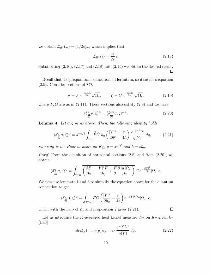
Recall that the prequantum connection is Hermitian, so it satisfies equation(2.9). Consider sections of HQ,

σ = F e−

s|Y |2

2~0

√Ωs, ζ = Ge

−s|Y |2

2~0

√Ωs, (2.19)

where F,G are as in (2.11). These sections also satisfy (2.9) and we have

〈δQ

∂∂s

σ, ζ〉Q = 〈δprQ

∂∂s

σ, ζ〉prQ. (2.20)

Lemma 4. Let σ, ζ be as above. Then, the following identity holds

〈δQ

∂∂s

σ, ζ〉Q = s−n/2∫

KC

¯FG ~0

( |Y |22~2

− n

4~

)e−|Y |2/~

η(Y )dg, (2.21)

where dg is the Haar measure on KC, g = xeiY and ~ = s~0.

Proof. From the definition of horizontal sections (2.8) and from (2.20), weobtain

〈δQ

∂∂s

σ, ζ〉Q =

∫

T ∗K

(∂F

∂s− |Y |2F

2~0+F

2

∂ ln |Ωs|∂s

)Ge

−s|Y |2

~0 |Ωs| ǫ.

We now use lemmata 1 and 3 to simplify the equation above for the quantumconnection to get,

〈δQ

∂∂s

σ, ζ〉Q =

∫

T ∗K

FG

( |Y |22~0

− n

4s

)e−s|Y |2/~0 |Ωs| ǫ,

which with the help of ψs and proposition 2 gives (2.21).

Let us introduce the K-averaged heat kernel measure dν~ on KC given by[Ha3]

dν~(g) = ν~(g) dg = c~

e−|Y |2/~

η(Y )dg, (2.22)

15

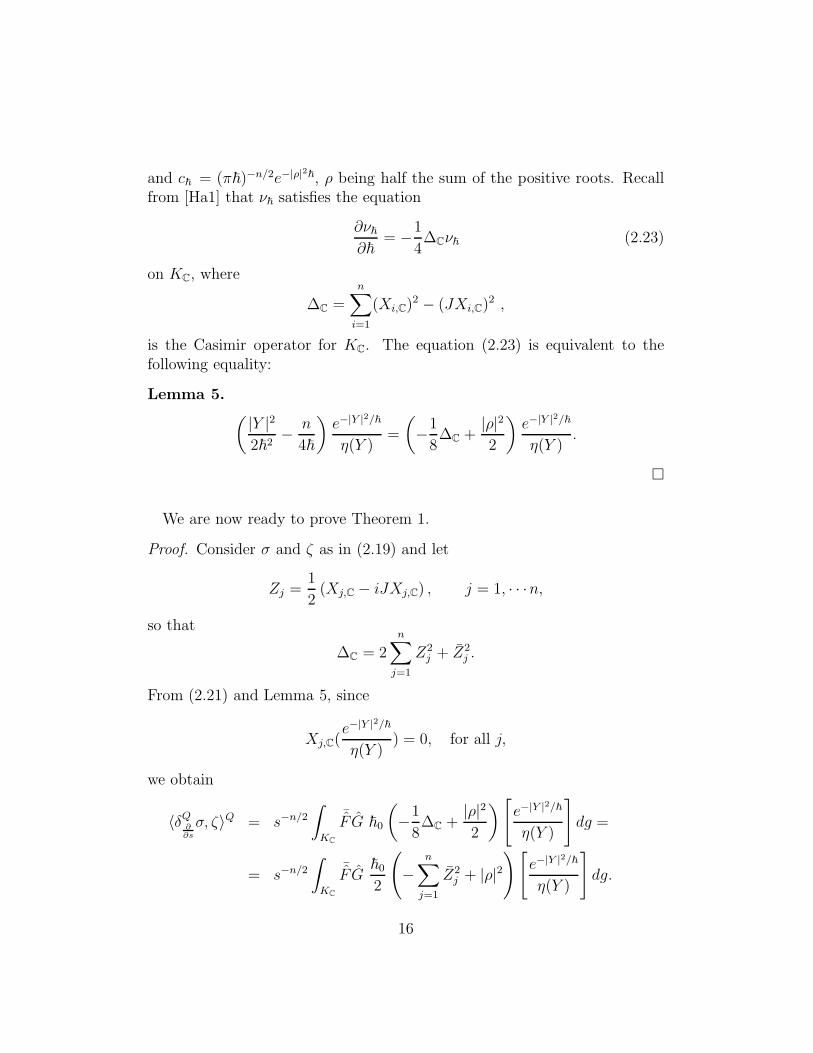
and c~ = (π~)−n/2e−|ρ|2~, ρ being half the sum of the positive roots. Recallfrom [Ha1] that ν~ satisfies the equation

∂ν~

∂~= −1

4∆Cν~ (2.23)

on KC, where

∆C =n∑

i=1

(Xi,C)2 − (JXi,C)2 ,

is the Casimir operator for KC. The equation (2.23) is equivalent to thefollowing equality:

Lemma 5.( |Y |2

2~2− n

4~

)e−|Y |2/~

η(Y )=

(−1

8∆C +

|ρ|22

)e−|Y |2/~

η(Y ).

We are now ready to prove Theorem 1.

Proof. Consider σ and ζ as in (2.19) and let

Zj =1

2(Xj,C − iJXj,C) , j = 1, · · ·n,

so that

∆C = 2

n∑

j=1

Z2j + Z2

j .

From (2.21) and Lemma 5, since

Xj,C(e−|Y |2/~

η(Y )) = 0, for all j,

we obtain

〈δQ∂∂s

σ, ζ〉Q = s−n/2∫

KC

¯FG ~0

(−1

8∆C +

|ρ|22

)[e−|Y |2/~

η(Y )

]dg =

= s−n/2∫

KC

¯FG

~0

2

(−

n∑

j=1

Z2j + |ρ|2

)[e−|Y |2/~

η(Y )

]dg.

16

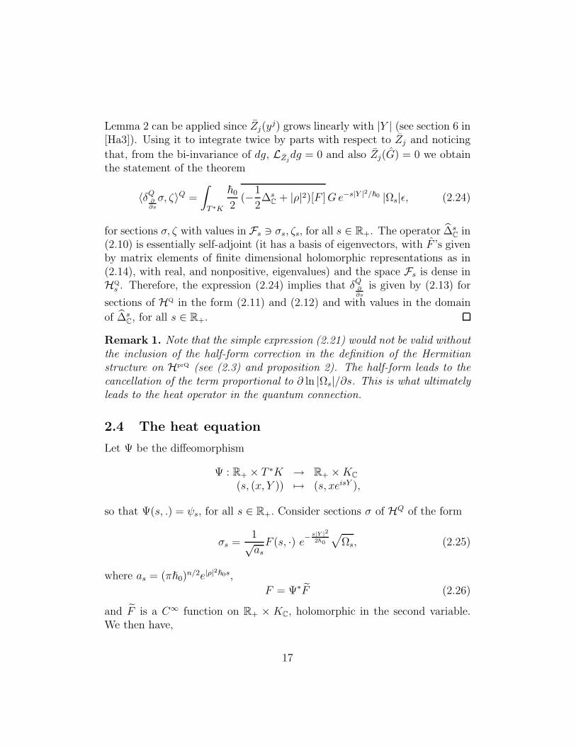
Lemma 2 can be applied since Zj(yj) grows linearly with |Y | (see section 6 in

[Ha3]). Using it to integrate twice by parts with respect to Zj and noticing

that, from the bi-invariance of dg, LZjdg = 0 and also Zj(G) = 0 we obtain

the statement of the theorem

〈δQ∂∂s

σ, ζ〉Q =

∫

T ∗K

~0

2(−1

2∆s

C+ |ρ|2)[F ]Ge−s|Y |2/~0 |Ωs|ǫ, (2.24)

for sections σ, ζ with values in Fs ∋ σs, ζs, for all s ∈ R+. The operator ∆sC

in(2.10) is essentially self-adjoint (it has a basis of eigenvectors, with F ’s givenby matrix elements of finite dimensional holomorphic representations as in(2.14), with real, and nonpositive, eigenvalues) and the space Fs is dense inHQ

s . Therefore, the expression (2.24) implies that δQ∂∂s

is given by (2.13) for

sections of HQ in the form (2.11) and (2.12) and with values in the domain

of ∆sC, for all s ∈ R+.

Remark 1. Note that the simple expression (2.21) would not be valid withoutthe inclusion of the half-form correction in the definition of the Hermitianstructure on HprQ (see (2.3) and proposition 2). The half-form leads to thecancellation of the term proportional to ∂ ln |Ωs|/∂s. This is what ultimatelyleads to the heat operator in the quantum connection.

2.4 The heat equation

Let Ψ be the diffeomorphism

Ψ : R+ × T ∗K → R+ ×KC

(s, (x, Y )) 7→ (s, xeisY ),

so that Ψ(s, .) = ψs, for all s ∈ R+. Consider sections σ of HQ of the form

σs =1√asF (s, ·) e−

s|Y |2

2ℏ0

√Ωs, (2.25)

where as = (πℏ0)n/2e|ρ|

2ℏ0s,

F = Ψ∗F (2.26)

and F is a C∞ function on R+ × KC, holomorphic in the second variable.We then have,

17

Theorem 2. A section of HQ of the form (2.25), (2.26) with σs in the

domain of ∆sC, for all s ∈ R+, is δQ-horizontal if and only if F is a solution

of the following heat equation on KC,

∂

∂sF =

ℏ0

4∆CF .

Proof. Substituting (2.25) in (2.13) we obtain

δQ∂∂s

σ = Ψ∗

(∂

∂sF − ℏ0

4∆CF

)e− s|Y |2

2ℏ0

√as

√Ωs.

Besides establishing the relation of the heat equation on complex semisim-ple Lie groups KC with the geometric quantization of T ∗K this result alsoprovides the link with the coherent state transform introduced by Hall in[Ha1].

Concerning the case K = U(1)n, note that the results in proposition 2 andequations (2.22) and (2.23) are still valid if we replace η(sY ) by 1 and theWeyl vector ρ by 0. Therefore, all the results above apply also to this case.

3 The quantum connection and the CST

The coherent state transform for K defines a parallel transport on a Hilbertbundle over R+ for an Hermitian connection that we denote by δH . In thissection we show that this parallel transport is naturally equivalent to the par-allel transport of the quantum connection δQ. This follows from propositions2 and 3, and from (2.3) and (2.22).

3.1 The CST connection - δH

Let ρ~, ~ > 0, be the heat kernel for the Laplacian ∆ on K associated tothe Ad-invariant inner product (· , ·) on K, ∆ =

∑ni=1X

2i . As proved in

[Ha1], ρ~ has a unique analytic continuation to KC, also denoted by ρ~. TheK-averaged coherent state transform (CST) is defined as the map

C~ : L2(K, dx) → H(KC)

(C~f)(g) =

∫

K

f(x)ρ~(x−1g) dx, f ∈ L2(K, dx), g ∈ KC, (3.1)

18

where dx is the normalized Haar measure on K. For each f ∈ L2(K, dx),C~f is the analytic continuation to KC of the solution of the heat equationon K,

∂u

∂~=

1

2∆u,

with initial condition given by u(0, x) = f(x). Therefore, C~f is given by

(C~f)(g) = (C ρ~ ⋆ f)(g) =(C e ~∆

2 f)

(g),

where ⋆ denotes the convolution in K and C denotes analytic continuationfrom K to KC. Recall that the K-averaged heat kernel measure dν~ on KC

is given by (2.22). Hall proves the following:

Theorem 3 (Hall). For each ~ > 0, the mapping C~ defined in (3.1) is anunitary isomorphism from L2(K, dx) onto the Hilbert space HL2(KC, dν~) :=L2(KC, dν~)

⋂H(KC).

This transformation defines a Hilbert vector bundle HH over the one-dimensional base R+ with global coordinate ~,

HH → R+

HH

~= HL2(KC, dν~).

which we call the CST bundle. The Hilbert space structure on the fibers ofHH is defined by

〈F~, G~〉H

~:=

∫

KC

F~(g)G~(g) dν~(g), F~, Gh ∈ HH

~.

From Theorem 3 we conclude that the operators

UH

~2~1= C~2

C−1~1

: HH

~1→ HH

~2(3.2)

define unitary transformations between the fibers which satisfy

UH

~3~2 UH

~2~1= UH

~3~1.

These operators correspond to the parallel transport with respect to an Her-mitian connection δH on HH. Let K denote the set of (equivalence class of)irreducible unitary representations of K. It follows from Theorem 3 that by

19

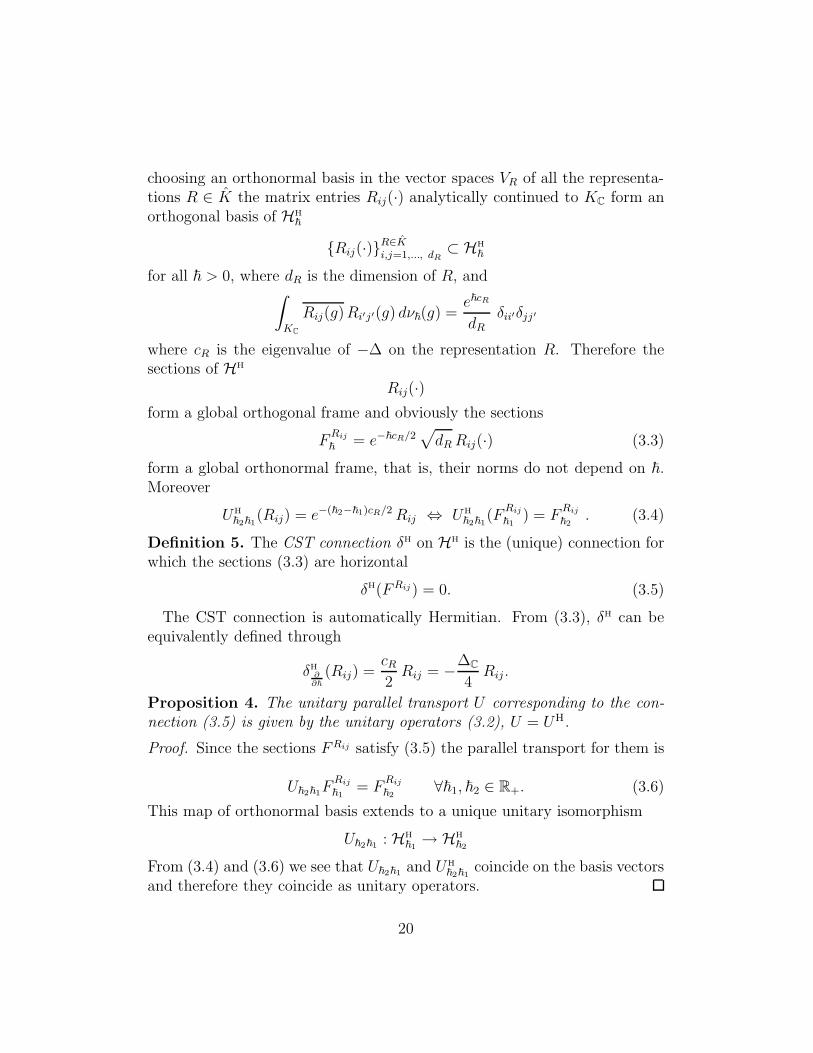
choosing an orthonormal basis in the vector spaces VR of all the representa-tions R ∈ K the matrix entries Rij(·) analytically continued to KC form anorthogonal basis of HH

~

Rij(·)R∈Ki,j=1,..., dR⊂ HH

~

for all ~ > 0, where dR is the dimension of R, and∫

KC

Rij(g)Ri′j′(g) dν~(g) =e~cR

dRδii′δjj′

where cR is the eigenvalue of −∆ on the representation R. Therefore thesections of HH

Rij(·)form a global orthogonal frame and obviously the sections

FRij

~= e−~cR/2

√dRRij(·) (3.3)

form a global orthonormal frame, that is, their norms do not depend on ~.Moreover

UH

~2~1(Rij) = e−(~2−~1)cR/2Rij ⇔ UH

~2~1(F

Rij

~1) = F

Rij

~2. (3.4)

Definition 5. The CST connection δH on HH is the (unique) connection forwhich the sections (3.3) are horizontal

δH(FRij) = 0. (3.5)

The CST connection is automatically Hermitian. From (3.3), δH can beequivalently defined through

δH∂

∂~

(Rij) =cR2Rij = −∆C

4Rij .

Proposition 4. The unitary parallel transport U corresponding to the con-nection (3.5) is given by the unitary operators (3.2), U = UH.

Proof. Since the sections FRij satisfy (3.5) the parallel transport for them is

U~2~1FRij

~1= F

Rij

~2∀~1, ~2 ∈ R+. (3.6)

This map of orthonormal basis extends to a unique unitary isomorphism

U~2~1: HH

~1→ HH

~2

From (3.4) and (3.6) we see that U~2~1and UH

~2~1coincide on the basis vectors

and therefore they coincide as unitary operators.

20

3.2 Equivalence between δH and δQ

Our main result in this section is

Theorem 4. The quantum connection δQ and the CST connection δH areequivalent in the sense that there exists a natural unitary isomorphismS : HH → HQ such that

δQ

∂∂~

S = S δH∂

∂~

. (3.7)

Proof. We start by constructing a natural unitary isomorphism between theCST bundle HH and the quantum bundle HQ. Let σ, ζ be two sections of HQ

of the form (2.11), (2.12),

σs = F (xeisY ) e− s|Y |2

2~0

√Ωs

ζs = G(xeisY ) e−

s|Y |2

2~0

√Ωs.

From proposition 2 we obtain

〈σs, ζs〉Q = as

∫

KC

F Gdν~ ,

where ~ = s~0 and as was defined in (2.25). Therefore, the bundle morphism

S~ : HH

~→ HQ

s

F 7→ ψ∗s(F ) e

−s|Y |2

2~0

√Ωs

as,

is a unitary isomorphism. To show (3.7) it is sufficient to see that the frameof horizontal sections

FRij = e−~cR/2Rij

is mapped to an horizontal frame. This follows directly from theorem 2.

Acknowledgements: We would also like to thank the referee forthe interest, the careful reading of the manuscript and useful suggestions.The authors were partially supported by the Center for Mathematics and

21

its Applications, IST (CF, PM and JM), the Multidisciplinary Center ofAstrophysics, IST (PM), the Center for Analysis, Geometry and DynamicalSystems, IST (JPN), and by the Fundacao para a Ciencia e a Tecnologia(FCT) through the programs PRAXIS XXI, POCTI, FEDER, the projectPOCTI/33943/MAT/2000, and the project CERN/FIS/43717/2001.

References

[AdPW] S.Axelrod, S.Della Pietra, E.Witten, “Geometric quantization of Chern-Simons gauge theory”, J. Diff. Geom. 33 (1991), 787-902.

[Fa] G.Faltings, “Stable G-bundles and projective connections”, J. AlgebraicGeom. 2 (1993) 507-568.

[FMMN] C.Florentino, P.Matias, J.Mourao, J.P.Nunes, “On the BKS pairing forKahler quantizations of the cotangent bundle of a Lie group”, in prepa-ration.

[FMN] C.Florentino, J.Mourao, J.P.Nunes, “Coherent state transform andabelian varieties”, J. Funct. Anal. 192 (2002) 410-424;“Coherent State Transforms and Vector Bundles on Elliptic Curves”, J.Funct. Anal. 204 (2003) 355-398.

[Ha1] B.C.Hall, “The Segal-Bargmann coherent state transform for compactLie groups”, J. Funct. Anal. 122 (1994), 103-151.

[Ha2] B.C.Hall, “Phase space bounds for quantum mechanics on a compact Liegroup”, Comm. Math. Phys. 184 (1997) 233-250;“Harmonic analysis with respect to the heat kernel measure”, Bull. Amer.Math. Soc. 38 (2001) 43-78.

[Ha3] B.C.Hall, “Geometric quantization and the generalized Segal-Bargmanntransform for Lie groups of compact type”, Comm. Math. Physics 226

(2002) 233-268;

[Hi] N.Hitchin, “Flat connections and geometric quantization”, Comm, Math.Phys. 131 (1990) 347-380.

[Las] Y. Laszlo, “Hitchin’s and WZW connections are the same”, J. DifferentialGeom. 49 (1998)547-576.

[Ra] T.R. Ramadas, “Faltings’ construction of the K-Z connection”, Comm.Math. Phys. 196 (1998) 133-143.

22

[Th1] T.Thiemann, “Reality Conditions Inducing Transforms for QuantumGauge Field Theory and Quantum Gravity”, Class. Quantum Grav. 13

(1996) 1383-1403.

[Th2] T.Thiemann, “Gauge Field Theory Coherent States I. General Proper-ties”, Class. quantum Grav. 18, 2025-2064.

[Wo] N. Woodhouse, “Geometric Quantization”, Clarendon Press, Oxford,1992.

†Department of Mathematics, Instituto Superior Tecnico, Av. Rovisco Pais, 1049-001 Lisboa, PortugalEmail: cfloren, jmourao, jpnunes@math.ist.utl.pt

‡Center for Mathematics and its Applications, Instituto Superior Tecnico, Av.Rovisco Pais, 1049-001 Lisboa, PortugalEmail: pmatias@math.ist.utl.pt

23