arX

iv:1

305.

4619

v1 [

quan

t-ph

] 2

0 M

ay 2

013

Bohmian quantum trajectories from coherent states

Bohmian quantum trajectories from coherent states

Sanjib Dey and Andreas Fring

Department of Mathematical Science, City University London,

Northampton Square, London EC1V 0HB, UK

E-mail: sanjib.dey.1@city.ac.uk, a.fring@city.ac.uk

Abstract: We find that real and complex Bohmian quantum trajectories resulting from

well-localized Klauder coherent states in the quasi-Poissonian regime possess qualitatively

the same type of trajectories as those obtained from a purely classical analysis of the corre-

sponding Hamilton-Jacobi equation. In the complex cases treated the quantum potential

results to a constant, such that the agreement is exact. For the real cases we provide

conjectures for analytical solutions for the trajectories as well as the corresponding quan-

tum potentials. The overall qualitative behaviour is governed by the Mandel parameter

determining the regime in which the wavefuntions evolve as soliton like structures. We

demonstrate these features explicitly for the harmonic oscillator and the Poschl-Teller

potential.

1. Introduction

Bohmian mechanics was originally proposed sixty years ago [1] to address some of the

difficulties present in the standard formulation of quantum mechanics based on the Copen-

hagen interpretation and its aim was to provide an alternative ontological view. Its central

purpose is to avoid the need for the collapse of the wavefunction and instead provide a

trajectory based scheme allowing for a causal interpretation. While this metaphysical dis-

cussion is still ongoing and is in parts very controversial [2, 3, 4], it needs to be stressed that

Bohmian mechanics leads to the same predictions of measurable quantities as the orthodox

framework. Here we will leave the interpretational issues aside and build on the fact that

the Bohmian formulation of quantum mechanics has undoubtedly proven to be a success-

ful technical tool for the study of some concrete physical scenarios. For instance, it has

been applied successfully to study of photodissociation problems [5], tunneling processes

[6], atom diffraction by surfaces [7, 8, 9] and high harmonic generation [10]. Whereas these

applications are mainly based on an analysis of real valued quantum trajectories, more

recently there has also been the suggestion [11, 12] for a formulation of Bohmian mechan-

ics based on complex trajectories. We will discuss here both versions, but it is this latter

Bohmian quantum trajectories from coherent states

formulation on which we will place our main focus and which will be the main subject of

our investigations in this manuscript.

Independently from the above suggestions, an alternative perspective on complex clas-

sical mechanics has recently emerged out of the study of complex quantum mechanical

Hamiltonians. It is by now well accepted that a large class of such systems constitute

well-defined self-consistent descriptions of physical systems [13, 14, 15] with real energy

eigenvalue spectra and unitary time-evolution. The dynamics of many classical models

has been investigated, for instance complex extensions of standard one particle systems

[16, 17, 18], non-Hamiltonian dynamical systems [19], chaotic systems [20] or deformations

of many-particle systems such as Calogero-Moser-Sutherland models [21, 22, 23, 24]. From

those studies conclusions were drawn for example with regard to tunneling behaviour [18]

or the existence of band structures [25]. It was also shown [26] that complex solutions to

a large class of complex quantum mechanical systems arise as special cases from the study

of Korteweg-deVries type of field equations, see [27] for a review on new models obtained

from deformations of integrable systems.

It is therefore natural to compare these two formulations and address the question

of whether they are equivalent in some regime. We will demonstrate here that this is

indeed the case, since the complex Bohmian quantum mechanics based on so-called Klauder

coherent states [28, 29, 30, 31] in the quasi-Poissonian regime is identical to a purely classical

study of the Hamilton-Jacobi equations.

Our manuscript is organized as follows: In section two we recall the basic equations

of Bohmian mechanics in the real as well as the complex case together with the main

features of Klauder coherent states. In section 3 we compare in both cases the trajectories

resulting from standard Gaussian wavepackets and those resulting from Klauder coherent

states with a purely classical treatment. For the latter case we verify the validity of a

conjectured formula for the trajectories. In section 4 we discuss the same scenario for the

Poschl-Teller potential. Our conclusions are stated in section 5

2. Real and complex Bohmian mechanics, Klauder coherent states

Let us briefly recall the key equations of Bohmian mechanics for reference purposes and

also to establish our conventions and notations. The starting point for the construction of

the Bohmian quantum trajectories is usually a solution of the time-dependent Schrodinger

equation involving a potential V (x)

i~∂ψ(x, t)

∂t= − ~

2

2m

∂2ψ(x, t)

∂x2+ V (x)ψ(x, t). (2.1)

The two variants leading either to real or complex trajectories are distinguished by different

parameterizations of the wavefunctions.

2.1 The real variant

The version based on real valued trajectories results from the WKB-polar decomposition

ψ(x, t) = R(x, t)ei/~S(x,t), with R(x, t), S(x, t) ∈ R. (2.2)

– 2 –

Bohmian quantum trajectories from coherent states

Upon the substitution of (2.2) into (2.1) the real and imaginary part are identified as

St +(Sx)

2

2m+ V (x)− ~

2

2m

Rxx

R= 0, and mRt +RxSx +

1

2RSxx = 0, (2.3)

usually referred to as the quantum Hamilton-Jacobi equation and the continuity equation,

respectively. When considering these equations from a classical point of view, the second

term in the first equation of (2.3) is interpreted as the kinetic energy such that the real

velocity v(t) and the last term, the so-called quantum potential Q(x, t), result to

mv(x, t) = Sx =~

2i

[

ψ∗ψx − ψψ∗

x

ψ∗ψ

]

, Q(x, t) = − ~2

2m

Rxx

R=

~2

4m

[

(ψ∗ψ)2x2 (ψ∗ψ)2

− (ψ∗ψ)xxψ∗ψ

]

,

(2.4)

respectively. The corresponding time-dependent effective potential is therefore Veff(x, t) =

V (x) + Q(x, t). Then one has two options to compute quantum trajectories. One can

either solve directly the first equation in (2.4) for x(t) or employ the effective potential Veffsolving mx = −∂Veff/∂x instead. Due to the different order of the differential equations

to be solved, we have then either one or two free parameter available. Thus for the two

possibilities to coincide the initial momentum is usually not free of choice, but the initial

position x(t = 0) = x0 is the only further input. The connection to the standard quantum

mechanical description is then achieved by computing expectation values from an ensemble

of n trajectories, e.g. 〈x(t)〉n = 1/n∑n

i=1xi(t).

2.2 The complex variant

In contrast, the version based on complex trajectories is computed from a parameterization

of the form

ψ(x, t) = ei/~S(x,t), with S(x, t) ∈ C. (2.5)

The substitution of (2.5) into (2.1) yields the single equation

St +(Sx)

2

2m+ V (x)− i~

2mSxx = 0. (2.6)

Interpreting this equation in a similar way as in the previous subsection, but now as a

complex quantum Hamilton-Jacobi equation, the second term in (2.6) yields a complex

velocity and the last term becomes a complex quantum potential

mv(x, t) = Sx =~

i

ψx

ψ, Q(x, t) = − i~

2mSxx = − ~

2

2m

[

ψxx

ψ− ψ2

x

ψ2

]

. (2.7)

The corresponding time-dependent effective potential is now Veff(x, t) = V (x) + Q(x, t).

Once again one has two options to compute quantum trajectories, either solving the first

equation in (2.7) for x(t), which is, however, now a complex variable. Alternatively, we

may also view the effective Hamiltonian Heff = p2/2m + Veff(x, t) = Hr + iHi in its own

right and simply compute the equations of motion directly from

xr =1

2

(

∂Hr

∂pr+∂Hi

∂pi

)

, xi =1

2

(

∂Hi

∂pr− ∂Hr

∂pi

)

, (2.8)

pr = −1

2

(

∂Hr

∂xr+∂Hi

∂xi

)

, pi =1

2

(

∂Hr

∂xi− ∂Hi

∂xr

)

, (2.9)

– 3 –

Bohmian quantum trajectories from coherent states

where we use the notations x = xr + ixi and p = pr + ipi with xr, xi, pr, pi ∈ R. For

the complex case the relation to the conventional quantum mechanical picture is less well

established although some versions have been suggested to extract real expectation values,

e.g. based on taking time-averaged mean values [32], seeking for isochrones [33, 34] or using

imaginary part of the velocity field of particles on the real axis [35].

We will here evaluate the expressions for the velocity, the quantum potential and

the resulting trajectories for two solvable potentials commencing with different choices of

solutions ψ. Our particular focus is here on commencing from coherent states and for that

reason we state their main properties.

2.3 Klauder coherent states

For Hermitian Hamiltonians H, with discrete bounded below and nondegenerate eigenspec-

trum En = ωen and orthonormal eigenstates |φn〉 the Klauder coherent states [28, 29, 30,

31] are defined in general as

ψJ(x, t) :=1

N (J)

∞∑

n=0

Jn/2 exp(−iωten)√ρn

φn(x), J ∈ R+0 . (2.10)

The probability distribution and the normalization constant are given by ρn :=∏n

k=1ek

and N 2(J) :=∑∞

k=0Jk/ρk, respectively. To allow for a more compact notation we adopt

the usual convention ρ0 = 1 throughout the manuscript. The key properties of these states

are their continuity in time and the variable J , the fact that they provide a resolution

of the identity and that they are temporarily stable satisfying the action angle identity

〈J, ωt|H |J, ωt〉 = ~ωJ .

Evidently the expression for ψJ(x, t) is only meaningful when the wave packet is

properly localized, i.e. the absolute value squared of the weighting function cn(J) =

Jn/2/N (J)√ρn needs to be peaked about some mean value 〈n〉 = 2Jd lnN (J)/dJ . The

deviation from a Poissonian distribution is captured in the so-called Mandel parameter [36]

defined as

Q :=∆n2

〈n〉 − 1 = Jd

dJln

d

dJlnN 2(J), (2.11)

with dispersion ∆n2 =⟨

n2⟩

− 〈n〉2. Here the case Q = 0 is a pure Poisson distribution

with Q < 0 and Q > 0 corresponding to sub-Poisson and super-Poisson distributions,

respectively. We refer to distributions with |Q| ≪ 1 as quasi-Poissonian.

3. The harmonic oscillator

The harmonic oscillator

Hho =p2

2m+

1

2mω2x2, (3.1)

constitutes a very instructive example on which many of the basic features can be under-

stood. We will therefore take it as a starting point. Many results may already be found

in the literature, but for completeness we also report them here together with some new

findings.

– 4 –

Bohmian quantum trajectories from coherent states

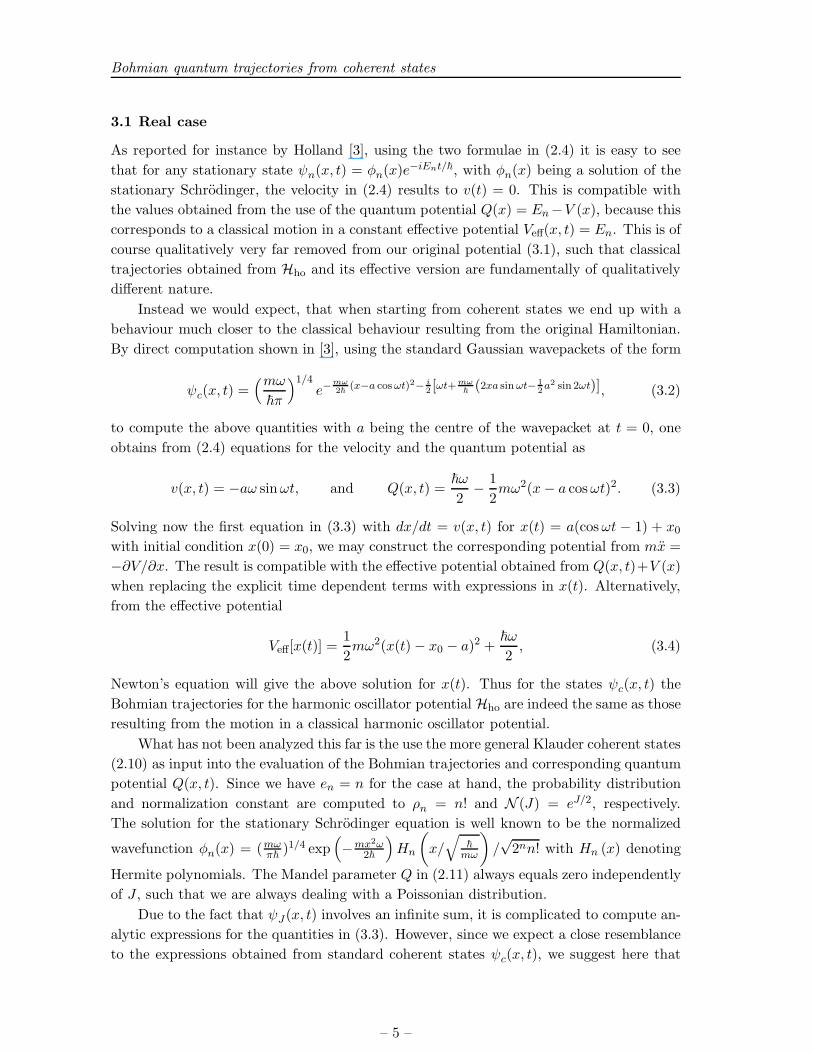
3.1 Real case

As reported for instance by Holland [3], using the two formulae in (2.4) it is easy to see

that for any stationary state ψn(x, t) = φn(x)e−iEnt/~, with φn(x) being a solution of the

stationary Schrodinger, the velocity in (2.4) results to v(t) = 0. This is compatible with

the values obtained from the use of the quantum potential Q(x) = En−V (x), because this

corresponds to a classical motion in a constant effective potential Veff(x, t) = En. This is of

course qualitatively very far removed from our original potential (3.1), such that classical

trajectories obtained from Hho and its effective version are fundamentally of qualitatively

different nature.

Instead we would expect, that when starting from coherent states we end up with a

behaviour much closer to the classical behaviour resulting from the original Hamiltonian.

By direct computation shown in [3], using the standard Gaussian wavepackets of the form

ψc(x, t) =(mω

~π

)1/4e−

mω

2~(x−a cosωt)2− i

2 [ωt+mω

~(2xa sinωt− 1

2a2 sin 2ωt)], (3.2)

to compute the above quantities with a being the centre of the wavepacket at t = 0, one

obtains from (2.4) equations for the velocity and the quantum potential as

v(x, t) = −aω sinωt, and Q(x, t) =~ω

2− 1

2mω2(x− a cosωt)2. (3.3)

Solving now the first equation in (3.3) with dx/dt = v(x, t) for x(t) = a(cosωt − 1) + x0with initial condition x(0) = x0, we may construct the corresponding potential from mx =

−∂V/∂x. The result is compatible with the effective potential obtained from Q(x, t)+V (x)

when replacing the explicit time dependent terms with expressions in x(t). Alternatively,

from the effective potential

Veff[x(t)] =1

2mω2(x(t)− x0 − a)2 +

~ω

2, (3.4)

Newton’s equation will give the above solution for x(t). Thus for the states ψc(x, t) the

Bohmian trajectories for the harmonic oscillator potential Hho are indeed the same as those

resulting from the motion in a classical harmonic oscillator potential.

What has not been analyzed this far is the use the more general Klauder coherent states

(2.10) as input into the evaluation of the Bohmian trajectories and corresponding quantum

potential Q(x, t). Since we have en = n for the case at hand, the probability distribution

and normalization constant are computed to ρn = n! and N (J) = eJ/2, respectively.

The solution for the stationary Schrodinger equation is well known to be the normalized

wavefunction φn(x) = (mωπ~ )

1/4 exp(

−mx2ω2~

)

Hn

(

x/√

~

mω

)

/√2nn! with Hn (x) denoting

Hermite polynomials. The Mandel parameter Q in (2.11) always equals zero independently

of J , such that we are always dealing with a Poissonian distribution.

Due to the fact that ψJ(x, t) involves an infinite sum, it is complicated to compute an-

alytic expressions for the quantities in (3.3). However, since we expect a close resemblance

to the expressions obtained from standard coherent states ψc(x, t), we suggest here that

– 5 –

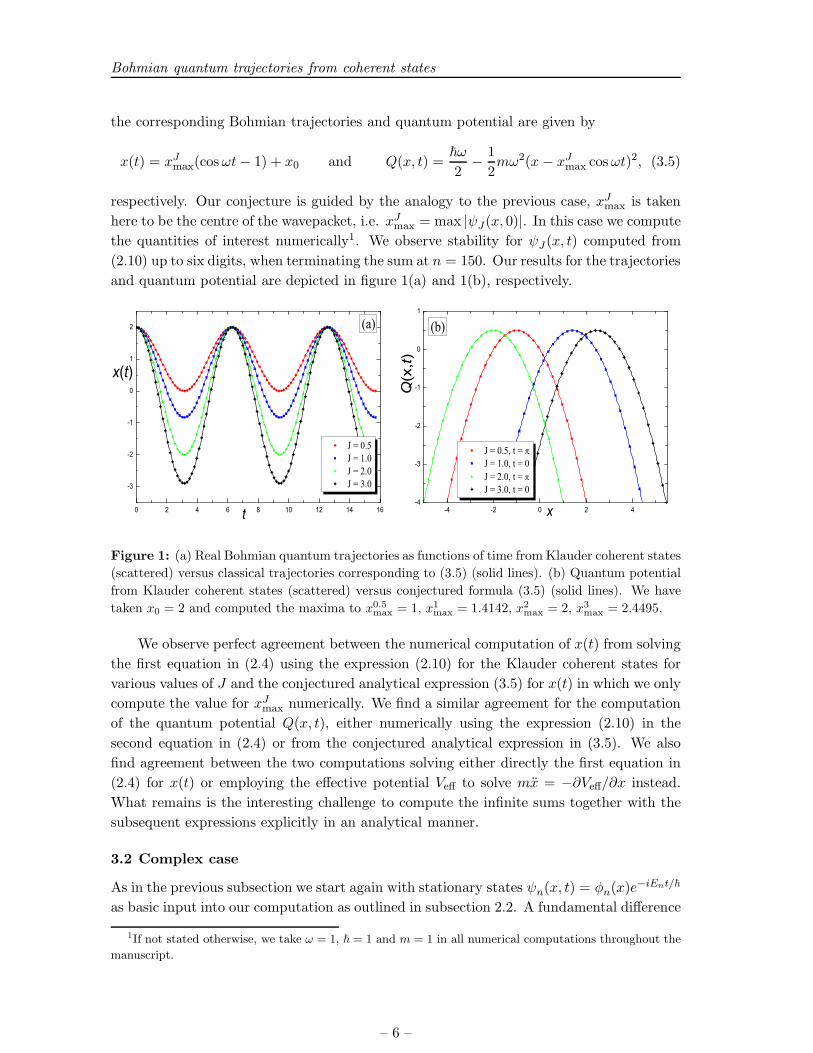
Bohmian quantum trajectories from coherent states

the corresponding Bohmian trajectories and quantum potential are given by

x(t) = xJmax(cosωt− 1) + x0 and Q(x, t) =~ω

2− 1

2mω2(x− xJmax cosωt)

2, (3.5)

respectively. Our conjecture is guided by the analogy to the previous case, xJmax is taken

here to be the centre of the wavepacket, i.e. xJmax = max |ψJ(x, 0)|. In this case we compute

the quantities of interest numerically1. We observe stability for ψJ(x, t) computed from

(2.10) up to six digits, when terminating the sum at n = 150. Our results for the trajectories

and quantum potential are depicted in figure 1(a) and 1(b), respectively.

0 2 4 6 8 10 12 14 16

-3

-2

-1

0

1

2 (a)

J = 0.5 J = 1.0 J = 2.0 J = 3.0

x(t)

t -4 -2 0 2 4-4

-3

-2

-1

0

1

(b)

J = 0.5, t = J = 1.0, t = 0 J = 2.0, t = J = 3.0, t = 0

Q(x

,t)

x

Figure 1: (a) Real Bohmian quantum trajectories as functions of time from Klauder coherent states

(scattered) versus classical trajectories corresponding to (3.5) (solid lines). (b) Quantum potential

from Klauder coherent states (scattered) versus conjectured formula (3.5) (solid lines). We have

taken x0 = 2 and computed the maxima to x0.5max = 1, x1max = 1.4142, x2max = 2, x3max = 2.4495.

We observe perfect agreement between the numerical computation of x(t) from solving

the first equation in (2.4) using the expression (2.10) for the Klauder coherent states for

various values of J and the conjectured analytical expression (3.5) for x(t) in which we only

compute the value for xJmax numerically. We find a similar agreement for the computation

of the quantum potential Q(x, t), either numerically using the expression (2.10) in the

second equation in (2.4) or from the conjectured analytical expression in (3.5). We also

find agreement between the two computations solving either directly the first equation in

(2.4) for x(t) or employing the effective potential Veff to solve mx = −∂Veff/∂x instead.

What remains is the interesting challenge to compute the infinite sums together with the

subsequent expressions explicitly in an analytical manner.

3.2 Complex case

As in the previous subsection we start again with stationary states ψn(x, t) = φn(x)e−iEnt/~

as basic input into our computation as outlined in subsection 2.2. A fundamental difference

1If not stated otherwise, we take ω = 1, ~ = 1 and m = 1 in all numerical computations throughout the

manuscript.

– 6 –

Bohmian quantum trajectories from coherent states

to the real case is that now we do not obtain a universal answer for all models. From (2.7)

we compute

v0(x, t) = iωx, Q0(x, t) =~ω

2, (3.6)

v1(x, t) = iωx− i~

mx, Q1(x, t) =

~ω

2+

~2

2mx2. (3.7)

As discussed in [37], for n = 1, 2 the explicit analytical solutions may be found in these

cases. By direct integration of the first equations in (3.6), (3.7) or from mx = −∂Veff/∂xwe compute

x0(t) = x0eiωt, and x1(t) = ±

√

~

mω+ e2itω

(

x20 −~

mω

)

. (3.8)

For larger values of n we obtain more complicated equations for the velocities and quantum

potentials, which may be solved numerically for x(t), see also [37, 38]. For instance, we

obtain from (2.7)

v5(x, t) = ixω − 5i~

mx+

60i~3 − 40i~2mx2ω

15~2mx− 20~m2x3ω + 4m3x5ω2, (3.9)

Q5(x, t) =~(

225~5 + 225~4mx2ω + 200~2m3x6ω3 − 80~m4x8ω4 + 16m5x10ω5)

2m (15~2x− 20~mx3ω + 4m2x5ω2)2(3.10)

The solutions for x1(t) and x5(t) are depicted in figure 2.

-1.5 -1.0 -0.5 0.0 0.5 1.0 1.5-0.75

-0.50

-0.25

0.00

0.25

0.50

0.75

(a) x0 = 1.5

x0 = 1.45

x0

0.1 x

00.75

x0

0.5

x1(t)

t -3 -2 -1 0 1 2 3-0.75

-0.50

-0.25

0.00

0.25

0.50

0.75

(b) x0 = 3.1

x0 = 3.04

x0

0.3 x

00.8

x0

2.5 x

01.6

x0

1.8x5(t)

t

Figure 2: Complex Bohmian quantum trajectories as functions of time for different initial values

x0 resulting from stationary states ψ1(x, t) and ψ

5(x, t) in panel (a) and (b), repectively.

In both cases we observe that the fixed points, at ±1 for v1(x, t) and at ±0.476251,

±1.47524, ±2.75624 for v5(x, t), are centres surrounded by closed limit cycles. For large

enough initial values we also observe bounded motion surrounding all fixed points.

Next we use once more the Gaussian wavepackets (3.2) as input to evaluate the velocity

and the quantum potential from (2.7)

v(x, t) = −ω(xi + a sinωt) + iω(xr − a cosωt), and Q(x, t) =~ω

2, (3.11)

– 7 –

Bohmian quantum trajectories from coherent states

The value for the constant quantum potential was also found in [34]. Solving now the

equation of motion with v(t) for xr and xi we obtain a complex trajectory

x(t) =(a

2+ c1

)

cosωt− c2 sinωt+ i[

c2 cosωt+(

c1 −a

2

)

sinωt]

, (3.12)

with integration constants c1 and c2. We compare this with the classical result computed

from the complex effective Hamiltonian

Heff =1

2m(p2r − p2i ) +

mω2

2(x2r − x2i ) + i

(

1

mprpi +mω2xrxi

)

+~ω

2. (3.13)

We may think of this Hamiltonian as being PT -symmetric, where the symmetry is induced

by the complexification and realized as PT : xr → −xr, xi → xi, pr → pr, pi → −pi,i→ −i. The equations of motion are then computed according to (2.8) and (2.9) to

xr =prm, xi =

pim, pr = −mω2xr, and pi = −mω2xi. (3.14)

As these equations decouple, they are easily solved. We find

x(t) = xr(0) cos ωt+pr(0)

mωsinωt+ i

[

xi(0) cos ωt+pi(0)

mωsinωt

]

. (3.15)

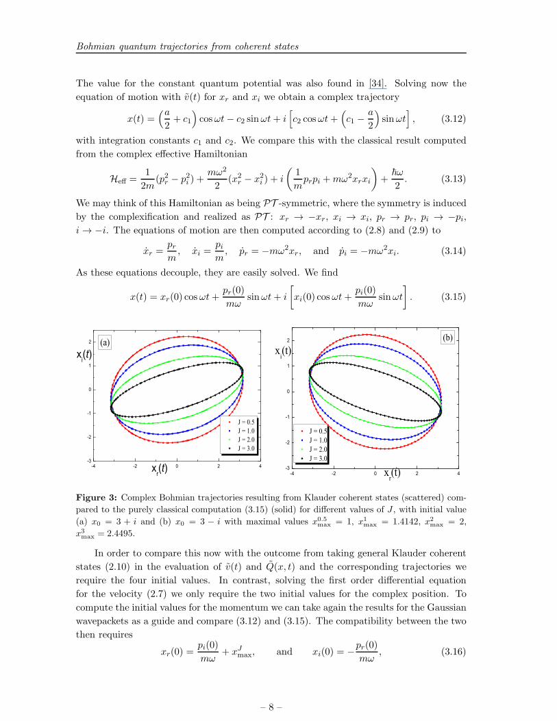
-4 -2 0 2 4-3

-2

-1

0

1

2 (a)xi(t)

xr(t)

J = 0.5 J = 1.0 J = 2.0 J = 3.0

-4 -2 0 2 4-3

-2

-1

0

1

2

xi(t)

xr(t)

J = 0.5J = 1.0J = 2.0J = 3.0

(b)

Figure 3: Complex Bohmian trajectories resulting from Klauder coherent states (scattered) com-

pared to the purely classical computation (3.15) (solid) for different values of J , with initial value

(a) x0 = 3 + i and (b) x0 = 3 − i with maximal values x0.5max = 1, x1max = 1.4142, x2max = 2,

x3max

= 2.4495.

In order to compare this now with the outcome from taking general Klauder coherent

states (2.10) in the evaluation of v(t) and Q(x, t) and the corresponding trajectories we

require the four initial values. In contrast, solving the first order differential equation

for the velocity (2.7) we only require the two initial values for the complex position. To

compute the initial values for the momentum we can take again the results for the Gaussian

wavepackets as a guide and compare (3.12) and (3.15). The compatibility between the two

then requires

xr(0) =pi(0)

mω+ xJmax, and xi(0) = −pr(0)

mω, (3.16)

– 8 –

Bohmian quantum trajectories from coherent states

where we have replaced a by xJmax. We can now either simply solve this for the initial values

for the momentum (3.16) or alternatively use directly the same initial values obtained from

the solution of (2.7). Comparing the direct parametric plot of (3.15) for the stated initial

conditions with the numerical computation of the complex Bohmian trajectories resulting

from Klauder coherent states, we find perfect agreement as depicted in figure 3.

Thus under these constraints for the initial conditions the trajectories resulting from

a classical analysis of the effective Hamiltonian (3.13) and the integration of the complex

Bohmian trajectories resulting from Klauder coherent states are identical. Notice that the

quantum nature of Heff is only visible in form of the overall constant ~ω/2, which does,

however, not play any role in the computation of the equations of motion.

4. The Poschl-Teller potential

Next we discuss the Bohmian trajectories associated with the Poschl-Teller Hamiltonian

[39] of the form

HPT =p2

2m+V02

[

λ(λ− 1)

cos2(x/2a)+

κ(κ− 1)

sin2(x/2a)

]

− V02(λ+ κ)2 for 0 ≤ x ≤ aπ, (4.1)

with V0 = ~2/(4ma2). This model has been widely discussed in the mathematical physics

literature, e.g. [40, 31], since it has the virtue of being exactly solvable, classically as well

as quantum mechanically. For a given energy E a classical solution is known to be

x(t) = a arccos

[

α− β

2+√γ cos

(

√

2E

m

t

a

)]

, (4.2)

with α = λ(λ− 1)V0/E, β = κ(κ− 1)V0/E and γ = α2/4 + β2/4− αβ/2− α− β + 1. The

time dependent Schrodinger equation is solved by discrete eigenfunctions

ψn(x, t) =1√Nn

cosλ( x

2a

)

sinκ( x

2a

)

2F1

[

−n, n+ κ+ λ; k +1

2; sin2

( x

2a

)

]

e−iEnt/~

(4.3)

with 2F1 denoting the Gauss hypergeometric function. The corresponding energy eigen-

values and the normalization factor are given by

En =~2

2ma2n(n+ κ+ λ), Nn = a2nn!

Γ(κ+ 1/2)Γ(n + λ+ 1/2)

Γ(2n + 1 + λ+ κ)

n∏

l=1

n− 1 + l + κ+ λ

2l − 1 + 2κ,

(4.4)

respectively. We will use these solutions in what follows.

4.1 Real case

As in the previous case we start with the construction of the trajectories from stationary

states (4.3). Once again for the real case the computation is unspectacular in this case

since the velocity computed from (2.4) is v(t) = 0 and the corresponding quantum potential

results again simply to Q(x) = En − VPT(x), such that classical trajectories correspond to

a motion in a constant effective potential Veff(x, t) = En.

– 9 –

Bohmian quantum trajectories from coherent states

More interesting, and qualitatively very close to the classical behaviour, are the tra-

jectories resulting from the Klauder coherent states given by the general expression (2.10).

In this case the probability distribution is computed with en = n(n + κ + λ) to ρn =

n!(n + κ + λ)n, where (x)n := Γ(x + n)/Γ(x) denotes the Pochhammer symbol. With

these expressions the normalization constant results to a confluent hypergeometric func-

tion N 2(J) = 0F1 (1 + κ+ λ;J), from which we compute the Mandel parameter (2.11)

to

Q(J, κ+ λ) =J

2 + κ+ λ0F1 (3 + κ+ λ;J)

0F1 (2 + κ+ λ;J)− J

1 + κ+ λ0F1 (2 + κ+ λ;J)

0F1 (1 + κ+ λ;J). (4.5)

Using the relation between the confluent hypergeometric function and the modified Bessel

function this is easily converted into the expression found in [31]. We agree with the

finding therein that Q is always negative, but disagree with the statement that Q tends

to zero for large J for fixed κ, λ. Instead we argue that for fixed coupling constants the

Mandel parameter Q is a monotonically decreasing function of J with Q(0, κ + λ) = 0.

Assuming that the coherent states closely resemble a classical behaviour, we conjecture

here in analogy to the classical solution (4.2) that the quantum trajectories acquire the

general form

x(t) = a arccos

[

X+

2+X−

2cos

(

2πt

T

)]

, (4.6)

with X± = cos(x0/a) ± cos(xm/a), T denoting the period and xm = x(T/2) = max[x(t)].

Our conjecture is based on an extrapolation of the analysis of the relations between α and

β and functions of x(0) and x(T/2). The effective potential computed from (4.6) is then

of Poschl-Teller type

Veff =2ma2π2

T 2

[

cos2(x0/2a) cos2(xm/2a)

cos2(x/2a)+

sin2(x0/2a) sin2(xm/2a)

sin2(x/2a)

]

. (4.7)

As in the previous case we will compute the quantum trajectories numerically2. Our

results from solving (2.4) are depicted in figure 4.

Most importantly we observe that the behaviour of the trajectories is entirely controlled

by the values of the Mandel parameter Q. Panel (a) and (b) show trajectories for different

values of J with pairwise identical values of the Mandel parameter, that is Q(2, 190) =

Q(0.0022906, 5) = −0.000054529, Q(0.5, 190) = Q(0.00057265, 5) = −0.000013634 and

Q(0.1, 190) = Q(0.000114531, 5) = −2.72691 × 10−6. We notice that the overall quali-

tative behaviour is simply rescaled in time. We further observe a small deviation from

the periodicity growing with increasing time. As a consequence the matching between the

quantum trajectories obtained from solving (2.4) and our conjectured analytical expression

(4.6) is good for small values of time, but worsens as time increases. The agreement im-

proves the closer the Mandel parameter approaches the Poissonian distribution, i.e. Q = 0.

Once the Mandel parameter becomes very negative the correlation between the classical

motion and the Bohmian trajectories is entirely lost as shown in panel (c) of figure 4 for

2We take a = 2 in all numerical computations in this section.

– 10 –

Bohmian quantum trajectories from coherent states

0.0 0.2 0.4 0.6 0.8 1.02.00

2.01

2.02

2.03

2.04

2.05 (a)

J = 2.0 J = 0.5 J = 0.1

x(t)

t 0 5 10 15 20 25 302.00

2.01

2.02

2.03

2.04

2.05

2.06 (b)

J = 0.0022906 J = 0.00057265 J = 0.000114531

x(t)

t

0 5 10 15 20 252

3

4

5

6

(c)

J = 20 J = 10 J = 2 J = 20.2846

x(t)

t 0 5 10 15 20 251

2

3

4

5(d)

x0 = 4

x0 =

x0 = 2.5

x0 = 2

x0 = 1.5

x0 = 1

x(t)

t

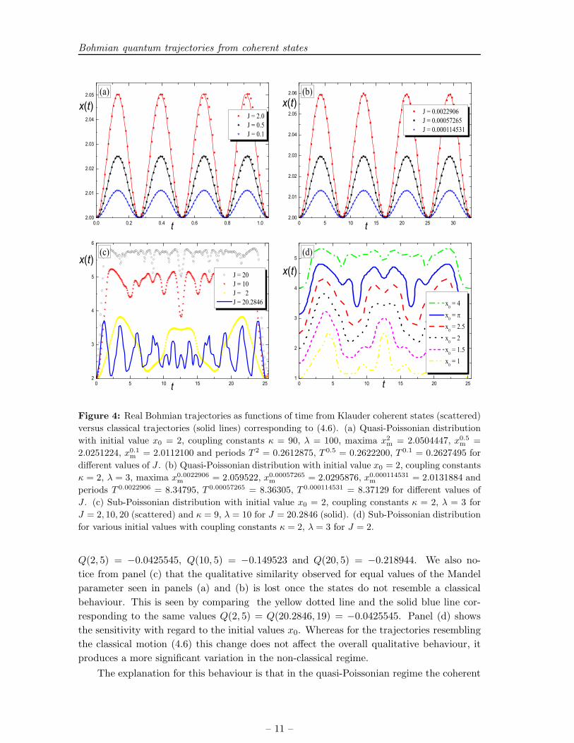
Figure 4: Real Bohmian trajectories as functions of time from Klauder coherent states (scattered)

versus classical trajectories (solid lines) corresponding to (4.6). (a) Quasi-Poissonian distribution

with initial value x0 = 2, coupling constants κ = 90, λ = 100, maxima x2m = 2.0504447, x0.5m =

2.0251224, x0.1m

= 2.0112100 and periods T 2 = 0.2612875, T 0.5 = 0.2622200, T 0.1 = 0.2627495 for

different values of J . (b) Quasi-Poissonian distribution with initial value x0 = 2, coupling constants

κ = 2, λ = 3, maxima x0.0022906m

= 2.059522, x0.00057265m

= 2.0295876, x0.000114531m

= 2.0131884 and

periods T 0.0022906 = 8.34795, T 0.00057265 = 8.36305, T 0.000114531 = 8.37129 for different values of

J . (c) Sub-Poissonian distribution with initial value x0 = 2, coupling constants κ = 2, λ = 3 for

J = 2, 10, 20 (scattered) and κ = 9, λ = 10 for J = 20.2846 (solid). (d) Sub-Poissonian distribution

for various initial values with coupling constants κ = 2, λ = 3 for J = 2.

Q(2, 5) = −0.0425545, Q(10, 5) = −0.149523 and Q(20, 5) = −0.218944. We also no-

tice from panel (c) that the qualitative similarity observed for equal values of the Mandel

parameter seen in panels (a) and (b) is lost once the states do not resemble a classical

behaviour. This is seen by comparing the yellow dotted line and the solid blue line cor-

responding to the same values Q(2, 5) = Q(20.2846, 19) = −0.0425545. Panel (d) shows

the sensitivity with regard to the initial values x0. Whereas for the trajectories resembling

the classical motion (4.6) this change does not affect the overall qualitative behaviour, it

produces a more significant variation in the non-classical regime.

The explanation for this behaviour is that in the quasi-Poissonian regime the coherent

– 11 –

Bohmian quantum trajectories from coherent states

states evolve as soliton like structures keeping their shape carrying out a periodic motion

in time. In contrast, in the sub-Poissonian regime the motion is no longer periodic and the

initial Gaussian shape of the wave is dramatically changed under the evolution of time.

These features are demonstrated in figure 5.

0 1 2 3 4 5 60

1

2

3

t = 0, J=0.0022906 t = 0.65, J=0.0022906 t = 0, J=2 t = 4, J=2

(x,t)

2

x

(a)

0 1 2 3 4 5 60.0

0.2

0.4

0.6

0.8

t = 0t = 1t = 10t = 20t = 30

|(x

,t)|2

x

(b)

Figure 5: (a) Periodic soliton like motion in the quasi-Poissonian regime for κ = 90, λ = 100

(thin) and κ = 2, λ = 3 (broad) with Q = −0.000054529 identical in both cases. (b) Spreading

wave in the sub-Poissonian regime with Q = −0.0917752 for J = 5 and κ = 2, λ = 3.

In figure 6 we plot the uncertainty relations for comparison.

0 5 10 15 20 25

0.5100

0.5103

0.5106

0.5109

0.5112

x p

t

Q= -0.000054529 Q= -0.000013634 Q= -0.000002726

(a)

0.0 0.4 0.8 1.2

0.5000055

0.5000070

0 5 10 15 20 250

1

2

3

4

5

6

7

Q= -0.307593 Q= -0.149523 Q= -0.042555

x p

t

(b)

Figure 6: Product of the position and momentum uncertainty as functions of time for different

values of the Mandel parameter Q. (a) The coupling constants are κ = 2, λ = 3, with J = 0.0022906

(red dotted), J = 0.00057265 (black dashed), J = 0.000114531 (blue solid) and J = 0.1 for the

subpanel with κ = 90, λ = 100. (b) The coupling constants are κ = 2, λ = 3 with J = 2 (red

dotted), J = 10 (black dashed) and J = 50 (blue solid).

In panel (a) we observe that in the quasi-Poissonian regime the saturation level is

almost reached with ∆x∆p being very close to ~/2, oscillating around 0.5106 with a de-

viation of ±0.0006 and in the subpanel oscillating around 0.5000065 with a deviation of

±0.0000008. This is of course compatible with the very narrow soliton like structure ob-

served in figure 5 leading to a classical type of behaviour. However, in the sub-Poissonian

– 12 –

Bohmian quantum trajectories from coherent states

regime the uncertainty becomes larger, as seen in panel (b), corresponding to a spread out

wave behaving very non-classical.

4.2 Complex case

Let us now consider the complex Bohmian trajectories starting once again with the con-

struction from stationary states ψn(x, t) = φn(x)e−iEnt/~. For the lowest states we may

compute analytical expressions from (2.7) for the velocities

v0(x, t) =~[

(κ+ λ) cos(

xa

)

+ κ− λ]

i2am sin(

xa

) , (4.8)

v1(x, t) =~[

(2κ2 + κ) cot(

x2a

)

+ (2λ2 + λ) tan(

x2a

)

− (κ+ λ+ 1)(κ+ λ+ 2) sin(

xa

)]

i2am[

(κ+ λ+ 1) cos(

xa

)

+ κ− λ] ,

and the quantum potentials

Q0(x, t) = V0

[

(κ− λ) cos(

xa

)

+ κ+ λ]

sin2(

xa

) , (4.9)

Q1(x, t) =V02

[

4(κ+ λ+ 1)(

(κ− λ) cos(

xa

)

+ κ+ λ+ 1)

[

(κ+ λ+ 1) cos(

xa

)

+ κ− λ]2 +

κ

sin2(

x2a

) +λ

cos2(

x2a

)

]

.

We note that the quantum potential Q1(x, t) resembles a Poschl-Teller potential apart from

its first term. For n = 0 we solve (2.7) analytically for the trajectories

x0(t) = ±a arccos

[

(κ+ λ) cos(

x0a

)

+ κ− λ]

eiht(κ+λ)

2a2m + λ− κ

κ+ λ

. (4.10)

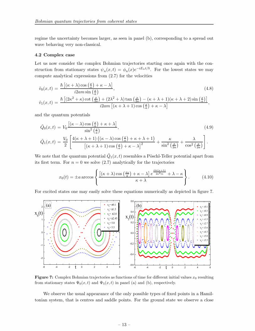
For excited states one may easily solve these equations numerically as depicted in figure 7.

-6 -4 -2 0 2 4 6

-2

-1

0

1

2x

0= ±0.1

x0= ±1.5

x0= ±2.0

x0= ±2.45

x0= 5.0

x0= 5.5

x0(t)

t

(a)

-6 -4 -2 0 2 4 6-0.6

-0.4

-0.2

0.0

0.2

0.4

0.6

x0= ±0.1x0= ±0.3x0= ±0.9x0= ±1.5x0= ±2.7x0= ±3.6x0= ±4.5x0= ±5.0x0= ±5.5

x5(t)

t

(b)

Figure 7: Complex Bohmian trajectories as functions of time for different initial values x0 resulting

from stationary states Ψ0(x, t) and Ψ5(x, t) in panel (a) and (b), respectively.

We observe the usual appearance of the only possible types of fixed points in a Hamil-

tonian system, that is centres and saddle points. For the ground state we observe a close

– 13 –

Bohmian quantum trajectories from coherent states

resemblance of the qualitative behaviour with the solution of the first excited state obtained

for the harmonic oscillator as shown in figure 2.

Unlike the trajectories resulting from coherent states those obtained from stationary

states are not expected to have a similar behaviour to the purely classical ones obtained

from solving directly the equations of motion (2.8) and (2.9). Complexifying the variables

as specified after (2.8) and (2.9), we may split the Hamiltonian into its real and imaginary

part HPT = Hr + iHi with

Hr =p2r − p2i2m

+ V0

[

(λ2 − λ)[

cosh(

xi

a

)

cos(

xr

a

)

+ 1]

[

cosh(

xi

a

)

+ cos(

xr

a

)]

2− (κ2 − κ)

[

cosh(

xi

a

)

cos(

xr

a

)

− 1]

[

cos(

xr

a

)

− cosh(

xi

a

)]

2

]

−V02(λ+ κ)2,

Hi =piprm

+ V0

[

(λ2 − λ) sinh(

xi

a

)

sin(

xr

a

)

[

cosh(

xi

a

)

+ cos(

xr

a

)]2 − (κ2 − κ) sinh(

xi

a

)

sin(

xr

a

)

[

cos(

xr

a

)

− cosh(

xi

a

)]2

]

. (4.11)

This Hamiltonian also respects the aforementioned PT -symmetry PT : xr → −xr, xi → xi,

pr → pr, pi → −pi, i → −i. Contourplots of the potential are shown in figures 9 and 10

with the colourcode convention being associated to the spectrum of light decreasing from

red to violet. The corresponding equations of motion are easily computed from (2.8) and

(2.9), albeit not reported here as they are very lengthy, and solved numerically as shown

for some parameter choices in the figures 8, 9 and 10 as solid lines.

Let us now compare them with the complex Bohmian trajectories computed from the

Klauder coherent states (2.10). A previous initial attempt to compute these trajectories

has been made in [41], however, the preliminary computations presented there do not agree

with our findings. We start by depicting a case for the quasi-Poissonian distribution in

figure 8.

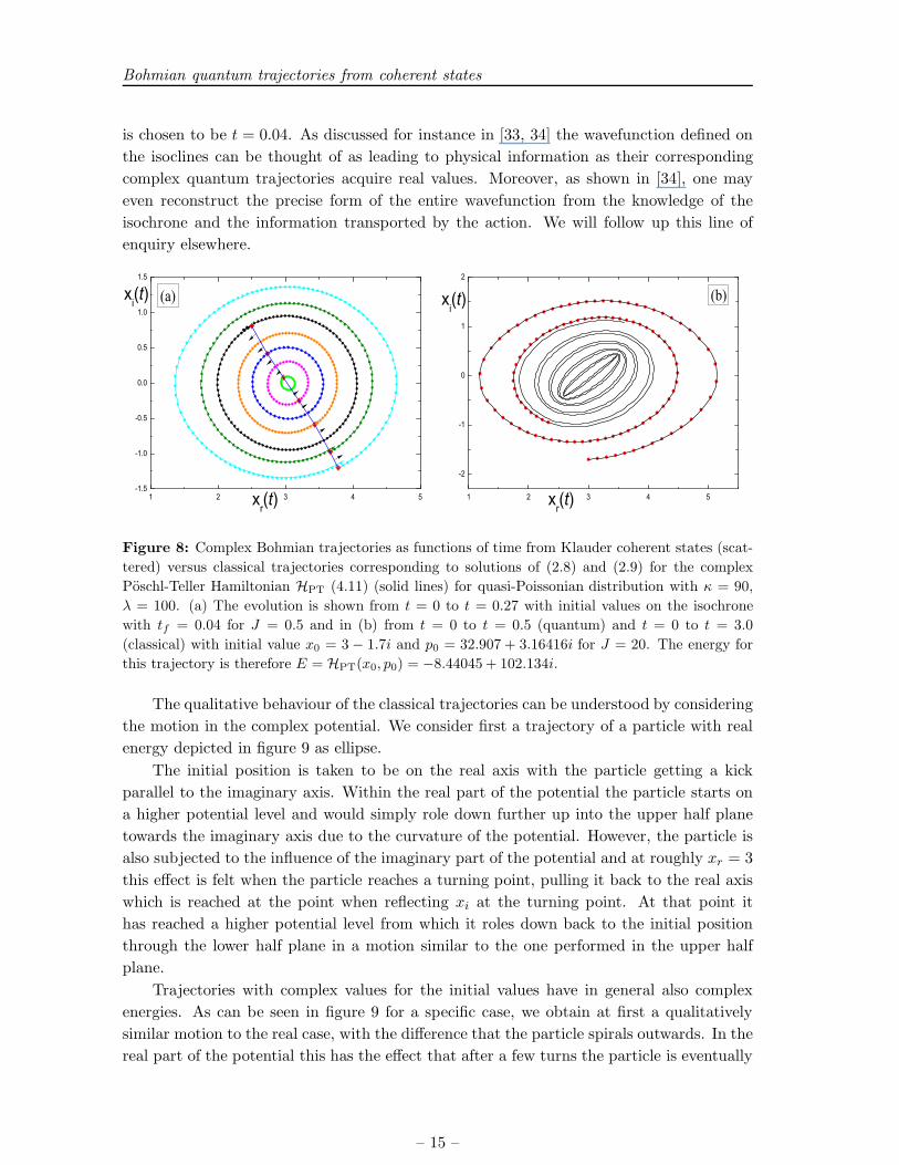
Remarkably, in that case we find a perfect match between these two entirely different

computations. We observe that unlike as for the real trajectories, for which we required an

effective potential to achieve agreement, these computations are carried out in both cases

for exactly the same coupling constants κ and λ with no adjustments made. Thus, just

as for the harmonic oscillator, this suggests that the complex quantum potential is simply

a constant such that the effective potential essentially coincides with the original one in

(4.1). From the trajectories with larger radii in panel (a) we observe that the trajectories

do not close and are not perfect ellipses. Prolonging the time beyond the cut-off time in

the panel (a) scenario we find inwardly spiralling trajectories. The coincidence between the

purely classical calculation and the quantum trajectories still persists for larger values of J

and more asymmetrical initial conditions closer to the boundary of the potential as shown

for an example in panel (b). For larger values of time we encounter numerical problems

due to the poor convergence of the series for large values of J .

Our initial values in 8(a) are chosen to lie on the isochrones, that is the set of all points

which when evolved in time will arrive all simultaneously, say at tf , on the real axis. The

isochrone is indicated in figure 8(a) by a red line and an additional arrow attached to it

pointing in the direction in which the real axis is reached. In our example the arrival time

– 14 –

Bohmian quantum trajectories from coherent states

is chosen to be t = 0.04. As discussed for instance in [33, 34] the wavefunction defined on

the isoclines can be thought of as leading to physical information as their corresponding

complex quantum trajectories acquire real values. Moreover, as shown in [34], one may

even reconstruct the precise form of the entire wavefunction from the knowledge of the

isochrone and the information transported by the action. We will follow up this line of

enquiry elsewhere.

1 2 3 4 5-1.5

-1.0

-0.5

0.0

0.5

1.0

1.5

(a)

xr(t)

xi(t)

1 2 3 4 5

-2

-1

0

1

2

(b)

xr(t)

xi(t)

Figure 8: Complex Bohmian trajectories as functions of time from Klauder coherent states (scat-

tered) versus classical trajectories corresponding to solutions of (2.8) and (2.9) for the complex

Poschl-Teller Hamiltonian HPT (4.11) (solid lines) for quasi-Poissonian distribution with κ = 90,

λ = 100. (a) The evolution is shown from t = 0 to t = 0.27 with initial values on the isochrone

with tf = 0.04 for J = 0.5 and in (b) from t = 0 to t = 0.5 (quantum) and t = 0 to t = 3.0

(classical) with initial value x0 = 3 − 1.7i and p0 = 32.907 + 3.16416i for J = 20. The energy for

this trajectory is therefore E = HPT(x0, p0) = −8.44045 + 102.134i.

The qualitative behaviour of the classical trajectories can be understood by considering

the motion in the complex potential. We consider first a trajectory of a particle with real

energy depicted in figure 9 as ellipse.

The initial position is taken to be on the real axis with the particle getting a kick

parallel to the imaginary axis. Within the real part of the potential the particle starts on

a higher potential level and would simply role down further up into the upper half plane

towards the imaginary axis due to the curvature of the potential. However, the particle is

also subjected to the influence of the imaginary part of the potential and at roughly xr = 3

this effect is felt when the particle reaches a turning point, pulling it back to the real axis

which is reached at the point when reflecting xi at the turning point. At that point it

has reached a higher potential level from which it roles down back to the initial position

through the lower half plane in a motion similar to the one performed in the upper half

plane.

Trajectories with complex values for the initial values have in general also complex

energies. As can be seen in figure 9 for a specific case, we obtain at first a qualitatively

similar motion to the real case, with the difference that the particle spirals outwards. In the

real part of the potential this has the effect that after a few turns the particle is eventually

– 15 –

Bohmian quantum trajectories from coherent states

Figure 9: Complex Bohmian quantum trajectories as functions of time from J = 0.5-Klauder

coherent states (scattered) versus classical trajectories (solid lines) corresponding to solutions of

(2.8) and (2.9) for the complex Poschl-Teller potential VPT (a) real part, (b) imaginary part for

quasi-Poissonian and localized distribution from t = 0 to t = 1.78 with κ = 90, λ = 100. The initial

values are x0 = 3 + 1.5i, p0 = −30.1922 + 0.385121i such that E = −6.55991 − 13.5182i (black

solid, red scattered) and x0 = 4.5, p0 = 41.8376i with real energy E = −31.7564 (blue solid, red

scattered).

attracted by the sink on top of the origin. The momentum it gains through this effect

propels it into the region with negative real part. Thus the particle has bypassed the infinite

potential barrier at the origin on the real axis, tunneling to the next potential minimum,

i.e. to the forbidden region in the real scenario. Similar effects have been observed in

the purely classical treatment of a complex elliptic potential in [18]. The continuation of

this trajectory and scenarios for other parameter choices can be understood in a similar

manner. For instance in figure 10 we depict a trajectory which does not spiral at first, but

the particle has instead already enough momentum that allows it to tunnel directly into

the negative region.

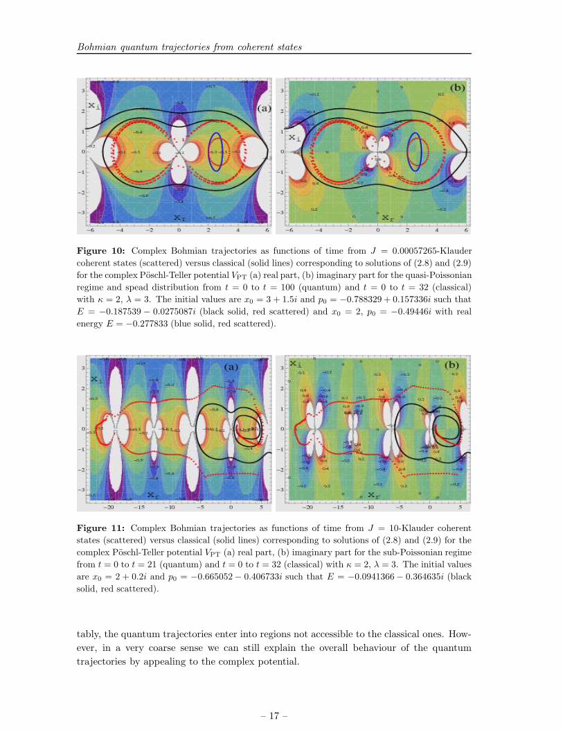
As in the real scenario the Mandel parameter controls the overall qualitative behaviour,

although in the complex case this worsens for non-real initial values that is complex ener-

gies. In quasi-Poissonian regime pictured in figure 8 and 9 we observe a complete match

between the purely classical and the quantum computation. However, this agreement ceases

to exist in figure 10, despite the fact that it is showing a quasi-Poissonian case with the

same value for Q. The difference is that in the latter case the wavefunction is less well

localized as we saw in figure 5. As can be seen in figure 10, for real energies we still have

the same qualitative behaviour, but for complex energies the less localized wave is spread

across a wide range of potential levels such that it can no longer mimic the same classical

motion. However, qualitatively we can see that in principle it is still compatible with the

motion in a complex classical Poschl-Teller potential.

As can be seen in figure 11 this resemblances ceases to exist when we enter the sub-

Poissonian regime.

We observe that the correlation between the two behaviours is now entirely lost. No-

– 16 –

Bohmian quantum trajectories from coherent states

Figure 10: Complex Bohmian trajectories as functions of time from J = 0.00057265-Klauder

coherent states (scattered) versus classical (solid lines) corresponding to solutions of (2.8) and (2.9)

for the complex Poschl-Teller potential VPT (a) real part, (b) imaginary part for the quasi-Poissonian

regime and spead distribution from t = 0 to t = 100 (quantum) and t = 0 to t = 32 (classical)

with κ = 2, λ = 3. The initial values are x0 = 3 + 1.5i and p0 = −0.788329 + 0.157336i such that

E = −0.187539 − 0.0275087i (black solid, red scattered) and x0 = 2, p0 = −0.49446i with real

energy E = −0.277833 (blue solid, red scattered).

Figure 11: Complex Bohmian trajectories as functions of time from J = 10-Klauder coherent

states (scattered) versus classical (solid lines) corresponding to solutions of (2.8) and (2.9) for the

complex Poschl-Teller potential VPT (a) real part, (b) imaginary part for the sub-Poissonian regime

from t = 0 to t = 21 (quantum) and t = 0 to t = 32 (classical) with κ = 2, λ = 3. The initial values

are x0 = 2 + 0.2i and p0 = −0.665052− 0.406733i such that E = −0.0941366− 0.364635i (black

solid, red scattered).

tably, the quantum trajectories enter into regions not accessible to the classical ones. How-

ever, in a very coarse sense we can still explain the overall behaviour of the quantum

trajectories by appealing to the complex potential.

– 17 –

Bohmian quantum trajectories from coherent states

5. Conclusions

We have computed real and complex quantum trajectories in two alternative ways, either by

solving the associated equation for the velocity or by solving the Hamilton-Jacobi equations

taking the quantum potential as a starting point. In all cases considered we found perfect

agreement for the same initial values in the position.

Our main concern in this manuscript has been to investigate the quality of the Klauder

coherent states and test how close they can mimic a purely classical description. This line

of enquiry continues our previous investigations [42, 43] for these type of states in a different

context. We have demonstrated that in the quasi-Poissonian regime well localized Klauder

coherent states produce the same qualitative behaviour as a purely classical analysis. We

found these features in the real as well as in the complex scenario. For the real trajectories

we conjectured some analytical expressions reproducing the numerically obtained results.

Whereas the real case required always some adjustments, we found for the complex analysis

of the harmonic oscillator and the Poschl-Teller potential a precise match with the purely

classical treatment.

Naturally there are a number of open problems left: Clearly it would be interesting to

produce more sample computations for different types of potentials, especially for the less

well explored complex case. In that case it would also be very interesting to explore further

how the conventional quantum mechanical description can be reproduced. Since Bohmian

quantum trajectories allow to establish that link there would be no need to guess any rules

in the classical picture mimicking some quantum behaviour as done in the literature.

Acknowledgments: SD is supported by a City University Research Fellowship. AF

thanks C. Figueira de Morisson Faria for useful discussions.

References

[1] D. Bohm, A Suggested interpretation of the quantum theory in terms of hidden variables. 1.,

Phys. Rev. 85, 166–179 (1952).

[2] B. Bohm and B. Hiley, The undivided universe: an ontological interpretation of quantum

theory, (Routledge, London) (1993).

[3] P. Holland, The Quantum Theory of Motion, An Account of the Broglie-Bohm Causal

Interpretation of Quantum Mechanics, (Cambridge University Press, Cambridge) (1993).

[4] B. J. Hiley, Bohmian Non-commutative Dynamics: History and Developments,

arXiv1303.6057 (2013).

[5] F. Sales Mayor, A. Askar, and H. Rabitz, Quantum fluid dynamics in the Lagrangian

representation and applications to photodissociation problems, J. Chem. Phys. 111, 2423(13)

(1999).

[6] C. Lopreore and R. Wyatt, Quantum Wave Packet Dynamics with Trajectories, Phys. Rev.

Lett. 82, 5190–5193 (1999).

[7] A. S. Sanz, F. Borondo, and S. Miret-Artes, Causal trajectories description of atom

diffraction by surfaces, Phys. Rev. B 61, 7743–7751 (2000).

– 18 –

Bohmian quantum trajectories from coherent states

[8] Z. Wang, G. Darling, and S. Holloway, Dissociation dynamics from a de Broglie-Bohm

perspective, J. Chem. Phys. 115, 10373(9) (2001).

[9] R. Guantes, A. Sanz, J. Margalef-Roig, and S. Miret-Artes, Atom-surface diffraction: a

trajectory description, Surface Science Reports 53, 199–330 (2004).

[10] A. Sanz, B. Augstein, J. Wu, and C. Figueira de Morisson Faria, Alternative interpretation

of high-order harmonic generation using Bohmian trajectories, arXiv:1205.529 (2012).

[11] R. Leacock and M. Padgett, Hamilton-Jacobi Theory and the Quantum Action Variable,

Phys. Rev. Lett. 50, 3–6 (1983).

[12] R. Leacock and M. Padgett, Hamilton-Jacobi/action-angle quantum mechanics, Phys. Rev.

D 28, 2491–2502 (1983).

[13] C. M. Bender and S. Boettcher, Real Spectra in Non-Hermitian Hamiltonians Having PT

Symmetry, Phys. Rev. Lett. 80, 5243–5246 (1998).

[14] C. M. Bender, Making sense of non-Hermitian Hamiltonians, Rept. Prog. Phys. 70, 947–1018

(2007).

[15] A. Mostafazadeh, Pseudo-Hermitian Representation of Quantum Mechanics, Int. J. Geom.

Meth. Mod. Phys. 7, 1191–1306 (2010).

[16] A. Nanayakkara, Classical trajectories of 1D complex non-Hermitian Hamiltonian systems,

J. Phys. A37, 4321–4334 (2004).

[17] C. M. Bender, D. D. Holm, and D. W. Hook, Complex Trajectories of a Simple Pendulum, J.

Phys. A40, F81–F90 (2007).

[18] C. M. Bender, D. W. Hook, and K. S. Kooner, Classical Particle in a Complex Elliptic

Potential, J. Phys. A43, 165201 (2010).

[19] C. M. Bender, D. D. Holm, and D. W. Hook, Complexified Dynamical Systems, J. Phys.

A40, F793–F804 (2007).

[20] C. M. Bender, J. Feinberg, D. W. Hook, and D. J. Weir, Chaotic systems in complex phase

space, Pramana J. Phys. 73, 453–470 (2009).

[21] A. Fring, A note on the integrability of non-Hermitian extensions of

Calogero-Moser-Sutherland models, Mod. Phys. Lett. 21, 691–699 (2006).

[22] A. Fring and M. Znojil, PT -Symmetric deformations of Calogero models, J. Phys. A40,

194010(17) (2008).

[23] P. E. G. Assis and A. Fring, From real fields to complex Calogero particles, J. Phys. A42,

425206(14) (2009).

[24] A. Fring and M. Smith, Antilinear deformations of Coxeter groups, an application to

Calogero models, J. Phys. A43, 325201(28) (2010).

[25] C. M. Bender and T. Arpornthip, Conduction bands in classical periodic potentials,

Pramana J. Phys. 73, 259–268 (2009).

[26] A. Cavaglia, A. Fring, and B. Bagchi, PT-symmetry breaking in complex nonlinear wave

equations and their deformations, J.Phys.A A44, 325201 (2011).

[27] A. Fring, PT-symmetric deformations of integrable models, Phil. Trans. Roy. Soc. Lond.

A371, 20120046 (2013).

– 19 –

Bohmian quantum trajectories from coherent states

[28] J. Klauder, Quantization without quantization, Annals Phys. 237, 147–160 (1995).

[29] J. Klauder, Coherent states for the hydrogen atom, J. Phys. A29, L293–L298 (1996).

[30] J.-P. Gazeau and J. R. Klauder, Coherent states for systems with discrete and continuous

spectrum, J. Phys. A 32, 123–132 (1999).

[31] J.-P. Antoine, J.-P. Gazeau, P. Monceau, J. R. Klauder, and K. A. Penson, Temporally

stable coherent states for infinite well and Poschl–Teller potentials, J. Math. Phys. 42,

2349–2387 (2001).

[32] C.-D. Yang, Trajectory interpretation of the uncertainty principle in 1D systems using

complex Bohmian mechanics, Phys.Lett. A 372, 6240–6253 (2008).

[33] Y. Goldfarb, I. Degani, and D. J. Tannor, Bohmian mechanics with complex action: A new

trajectory-based formulation of quantum mechanics, J. Chem. Phys. 125, 231103 (2006).

[34] C. Chou and R. E. Wyatt, Quantum trajectories in complex space, Phys. Rev. A 76, 012115

(2007).

[35] M. John, Probability and complex quantum trajectories, Annals of Physics 324, 220–231

(2009).

[36] L. Mandel, Sub-Poissonian photon statistics in resonance fluorescence, Opt. Lett. 4, 205–207

(1979).

[37] M. John, Modified de Broglie-Bohm approach to quantum mechanics, Found. Phys. Lett. 15,

329–343 (2002).

[38] C.-D. Yang, Modeling quantum harmonic oscillator in complex domain, Chaos, Solitons and

Fractals 30, 342–362 (2006).

[39] G. Poschl and E. Teller, Bemerkungen zur Quantenmechanik des anharmonischen

Oszillators, Z. Phys. 83, 143–151 (1933).

[40] H. Kleinert and I. Mustapic, Summing the spectral representations of Poschl–Teller and

Rosen-Morse fixed-energy amplitudes, J. Math. Phys. 33, 643(20) (1992).

[41] M. John and K. Mathew, Coherent States and Modified de Broglie-Bohm Complex Quantum

Trajectories, arXiv:1104.3197 (2011).

[42] S. Dey and A. Fring, Squeezed coherent states for noncommutative spaces with minimal

length uncertainty relations, Phys. Rev. D86, 064038 (2012).

[43] S. Dey, A. Fring, L. Gouba, and P. G. Castro, Time-dependent q-deformed coherent states

for generalized uncertainty relations, Phys. Rev. D 87, 084033 (2013).

– 20 –