arX

iv:c

ond-

mat

/040

7811

v1 [

cond

-mat

.sta

t-m

ech]

30

Jul 2

004

Quantum-Classical Limit of Quantum Correlation Functions

Alessandro Sergi1, ∗ and Raymond Kapral1, 2, †

1Chemical Physics Theory Group, Department of Chemistry,

University of Toronto, Toronto, ON M5S 3H6, Canada

2Fritz-Haber-Institut der Max-Planck-Gesellschaft, Faradayweg 4-6, 14195 Berlin, Germany

(Dated: 2nd February 2008)

A quantum-classical limit of the canonical equilibrium time correlation function for a quantum

system is derived. The quantum-classical limit for the dynamics is obtained for quantum systems

comprising a subsystem of light particles in a bath of heavy quantum particles. In this limit the

time evolution of operators is determined by a quantum-classical Liouville operator but the full equi-

librium canonical statistical description of the initial condition is retained. The quantum-classical

correlation function expressions derived here provide a way to simulate the transport properties

of quantum systems using quantum-classical surface-hopping dynamics combined with sampling

schemes for the quantum equilibrium structure of both the subsystem of interest and its environ-

ment.

I. INTRODUCTION

The dynamical properties of systems close to equilibrium may be described in terms of equilibrium time correlation

functions of dynamical variables or operators. For a quantum system with Hamiltonian H at temperature T with

volume V , linear response theory shows that the time correlation function of two operators A and B, needed to obtain

transport properties, has the Kubo transformed form [1, 2],

CAB(t; β) =1

β

∫ β

0

dλTrA(t)eλH B†e−λH ρe

=1

β

∫ β

0

dλ1

ZQTrB†e

ih

t∗1HAe−ih

t2H , (1)

where β = (kBT )−1, ρe = Z−1Q e−βH is the quantum canonical equilibrium density operator, ZQ = Tre−βH is the

canonical partition function and, in the second line, t1 = t− ih(β−λ) and t2 = t− ihλ. The evolution of the operator

∗asergi@chem.utoronto.ca

†rkapral@chem.utoronto.ca

2

A(t) is given by the solution of the Heisenberg equation of motion, dA(t)/dt = ih [H, A(t)], where the square brackets

denote the commutator.

While such correlation functions provide information on the transport properties of the system, their direct compu-

tation for condensed phase systems is not feasible due to our inability to simulate the quantum mechanical evolution

equations for systems with a large number of degrees of freedom. While approximate schemes have been devised

to treat quantum many body dynamics, for example, quantum mode coupling methods have proved useful in the

calculation of collective modes for some applications [3], we are primarily concerned with methods that approximate

the full many body evolution of the microscopic degrees of freedom. In many circumstances only a few degrees of

freedom need to be treated quantum mechanically (quantum subsystem) while the remainder of the system with which

they interact can be treated classically (classical bath) to a good approximation. Examples where such a description

is appropriate include proton and electron transfer processes occurring in solvents or other chemical environments

composed of heavy atoms. Quantum-classical methods have been reviewed by Egorov et al. [4] and one form of a

quantum-classical approximation has been assessed in the weak coupling limit where there is no feedback between the

quantum and classical subsystems. Although it is difficult to determine transport properties such as the reaction rate

constant from the full quantum time correlation function when the entire system is treated quantum mechanically,

methods are being developed to carry out such calculations. [5] Mixed quantum-classical methods also provide a route

to carry out nonadiabatic rate calculations.

A number of schemes have been proposed for carrying out quantum dynamics in classical environments. [6, 7, 8,

9, 10, 11, 12, 13] We focus on approaches where the evolution is described by a quantum-classical Liouville equation.

[14, 15, 16, 17, 18, 19, 20, 21] For a quantum system coupled to a classical environment it is possible to derive an

evolution equation for dynamical variables or operators (or the density matrix) by an expansion in a small parameter

that characterizes the mass ratio of the light and heavy particles in the system. The quantum-classical analog of the

Heisenberg equation of motion is, [21]

d

dtAW (X, t) =

i

h[HW , AW (t)] −

1

2

(

{HW , AW (t)} − {AW (t), HW })

= iLAW (X, t) . (2)

Here AW (X, t) is the partial Wigner representation [21, 22] of a quantum operator; it is still an operator in the Hilbert

space of the quantum subsystem but a function of the phase space coordinates X = (R, P ) of the classical bath. In

this equation {· · · , · · ·} is the Poisson bracket and L is the quantum-classical Liouville operator. A few features

of quantum-classical Liouville dynamics are worth noting. This equation of motion includes feedback between the

3

classical and quantum degrees of freedom. The environmental dynamics is fully classical only in the absence of

coupling to the quantum subsystem. In the presence of coupling the environmental evolution cannot be described

by Newtonian dynamics, although the simulation of the quantum-classical evolution can be formulated in terms of

classical trajectory segments. [21] For harmonic environmental potentials with bilinear coupling to the quantum

subsystem the evolution is equivalent to the fully quantum mechanical evolution of the entire system. Quantum-

classical simulations of the spin-boson model are in accord with the numerically exact quantum results [23] and have

been used to test quantum-classical simulation algorithms. [24, 25]

Equation (2) is valid in any basis and an especially convenient basis for simulating the evolution by surface-hopping

schemes is the adiabatic basis, {|α1; R >}, the set of eigenstates of the quantum subsystem Hamiltonian in the presence

of fixed classical particles. In this case the matrix elements of an operator Aα1α′

1

W (X, t) =< α1; R|AW (X, t)|α′1; R >

satisfy

d

dtA

α1α′

1

W (X, t) = i∑

β1β′

1

Lα1α′

1β1β′

1A

β1β′

1

W (X, t) , (3)

where Lα1α′

1β1β′

1denotes the representation of the quantum-classical Liouville operator in the adiabatic basis. [21]

This equation may be solved using surface-hopping schemes that combine a probabilistic description of the quantum

transitions interspersed with classical evolution trajectory segments. [24, 25, 26, 27, 28] Although further algorithm

development is needed to carry the simulations to arbitrarily long times, the quantum-classical evolution is not a

short time approximation to full quantum evolution. Rather, it is an approximation to the full quantum evolution

for arbitrary times since the quantum-classical evolution is derived at the level of the Liouville operator and not the

quantum propagator. Given the evolution equation (2) (and the corresponding quantum-classical Liouville equation

for the density matrix) one may construct a statistical mechanics of quantum-classical systems [29, 30] and compute

transport properties such as chemical rate constants [31] from the correlation functions obtained from this analysis.

In this article we consider another route to determine quantum-classical correlation functions for transport proper-

ties. We begin with the full quantum mechanical expression for the time correlation function (Eq. (1)) and take the

limit where the dynamics is determined by quantum-classical evolution equations for the spectral density that enters

the correlation function expression. While the calculations leading to our expression for the correlation function are

somewhat lengthy, the final result has a simple structure:

CAB(t; β) =∑

β′

1β1β′

2β2

∫

dX1dX2 B†β1β′

1

W (X1,t

2)

×Aβ2β′

2

W (X2,−t

2)W

β′

1β1β′

2β2(X1, X2; β) .

4

(4)

This expression for the time correlation function retains the full quantum statistical character of the initial condition

through the spectral density function W (Eq. (40) below) but the forward and backward time evolution of the

operators B†β1β′

1

W and Aβ2β′

2

W , respectively, is given by the solutions of the quantum-classical evolution equation (3).

Consequently, one may combine algorithms for determining quantum equilibrium properties with surface-hopping

algorithms for quantum-classical evolution to estimate the value of the correlation function. Quantum effects enter in

all orders in this expression for the correlation function. In addition to the fact that the initial value of the spectral

density contains the full quantum equilibrium statistics, since the quantum-classical Liouville operator appears in

the exponent in the propagator, the quantum-classical propagator contains all orders of h, albeit in an approximate

fashion.

The outline of the paper is as follows: In Sec. II we construct the partial Wigner representation of the quantum time

correlation function and obtain expressions for the spectral density and its matrix elements in an adiabatic basis. In

Sec. III we derive a quantum-classical evolution equation for the matrix elements of the spectral density and establish

a connection to quantum-classical Liouville evolution. The results of these two sections are used in Sec. IV to obtain

Eq. (4). In Sec. V we analyze the initial value of the spectral density in the high temperature limit. The conclusions

of the study are given in Sec. VI while additional details of the calculations are presented in the Appendices.

II. PARTIAL WIGNER REPRESENTATION OF QUANTUM CORRELATION FUNCTION

We consider quantum systems whose degrees of freedom can be partitioned into two subsets corresponding to light

(mass m) and heavy (mass M) particles, respectively. We use small and capital letters to denote operators for phase

points in the light and heavy mass subsystems, respectively. In this notation the Hamiltonian operator for the entire

system is the sum of the kinetic energy operators or the two subsystems and the potential energy of the entire system,

H = P 2/2M + p2/2m + V (q, Q).

We are interested in the limit where the dynamics of the heavy particle subsystem is treated classically and the light

particle subsystem retains its full quantum character. To this end it is convenient to take a partial Wigner transform

of the heavy degrees of freedom and represent the light degrees of freedom in some suitable basis.

In order to carry out this program we begin with the quantum mechanical Kubo transformed correlation function

and write the trace over the heavy subsystem degrees of freedom in the second line of Eq. (1) using a {Q} coordinate

5

representation,

CAB(t; β) =1

β

∫ β

0

dλ1

ZQTr′

∫ 4∏

i=1

dQi < Q1|B†|Q2 >< Q2|e

ih

t∗1H |Q3 >< Q3|A|Q4 >< Q4|e− i

ht2H |Q1 > . (5)

The prime in Tr′ refers to the fact that the trace is now only over the light particle subsystem degrees of freedom.

Making use of the change of variables, Q1 = R1 −Z1/2, Q2 = R1 + Z1/2, Q3 = R2 −Z2/2 and Q4 = R2 + Z2/2, this

equation may be written in the equivalent form,

CAB(t; β) =1

β

∫ β

0

dλ1

ZQTr′

∫ 2∏

i=1

dRidZi < R1 −Z1

2|B†|R1 +

Z1

2>< R1 +

Z1

2|e

ih

t∗1H |R2 −Z2

2>

× < R2 −Z2

2|A|R2 +

Z2

2>< R2 +

Z2

2|e−

ih

t2H |R1 −Z1

2> . (6)

The next step in the calculation is to replace the coordinate space matrix elements of the operators with their

representation in terms of Wigner transformed quantities. The partial Wigner transform of an operator is defined by

[21, 22]

AW (R2, P2) =

∫

dZ2eih

P2·Z2〈R2 −Z2

2|A|R2 +

Z2

2〉 , (7)

while the inverse transform is

〈R2 −Z2

2|A|R2 +

Z2

2〉 =

1

(2πh)νh

∫

dP2e− i

hP2·Z2AW (R2, P2) . (8)

Here νh is the dimension of the heavy mass subsystem. The partially Wigner transformed operator AW (X2) is

a function of the phase space coordinates X2 ≡ (R2, P2) and an operator in the Hilbert space of the quantum

subsystem. It is convenient to consider a representation of such operators in basis of eigenfunctions. In this paper

we use an adiabatic basis since, through this representation, we can make connection with surface-hopping dynamics.

The partial Wigner transform of the Hamiltonian H is HW = P 2/2M + p2/2m + VW (q, R) ≡ P 2/2M + hW (R).

The last equality defines the Hamiltonian hW (R) for the light mass subsystem in the presence of fixed particles

of the heavy mass subsystem. The adiabatic basis is determined from the solutions of the eigenvalue problem,

hW (R)|α; R >= Eα(R)|α; R >. The adiabatic representation of AW (X2) is,

AW (X2) =∑

α2α′

2

|α2; R2 > Aα2α′

2

W (X2) < α′2; R2| , (9)

where Aα2α′

2

W (X2) =< α2; R2|AW (X2)|α′2; R2 >.

By inserting Eq. (9) into Eq. (8) we can express the coordinate representation of the operator A as

< R2 −Z2

2|A|R2 +

Z2

2>=

1

(2πh)νh

∑

α2α′

2

∫

dP2 e−i2P2·Z2 |α2; R2 > A

α2α′

2

W (X2) < α′2; R2| . (10)

6

Then, substituting the result into Eq. (6) (along with a similar representation of the B† operator), we obtain,

CAB(t; β) =1

β

∫ β

0

dλ∑

α1,α′

1,α2,α′

2

∫ 2∏

i=1

dXi B†α1α′

1

W (X1)Aα2α′

2

W (X2)

× Wα′

1α1α′

2α2(X1, X2, t; β, λ) . (11)

Here we defined the matrix elements of the spectral density by

Wα′

1α1α′

2α2(X1, X2, t; β, λ) =1

ZQ

∫ 2∏

i=1

dZie− i

h(P1·Z1+P2·Z2) < α′

1; R1| < R1 +Z1

2|e

ih

t∗1H |R2 −Z2

2> |α2; R2 >

× < α′2; R2| < R2 +

Z2

2|e−

ih

t2H |R1 −Z1

2> |α1; R1 >

1

(2πh)2νh. (12)

Our task is now to find an evolution equation for Wα′

1α1α′

2α2(X1, X2, t; β, λ) in the mixed quantum-classical limit.

Before doing this we observe that the expression for the quantum correlation function in the partial Wigner represen-

tation is equivalent to an expression involving full Wigner transforms of the operators.

A. Relation to full Wigner representation

Since the correlation function is independent of the representation we choose for the light and heavy mass sub-

systems, we may also represent the light mass subsystem in terms of a Wigner transform instead of a set of basis

functions. To establish the connection between these two forms of the correlation function we note that the full

Wigner transform of the the operator A is given by

AW (x2, X2) =

∫

dz2 eih

p2·z2 < r2 −z2

2|AW (X2)|r2 +

z2

2> ,

=∑

α2α′

2

∫

dz2 eih

p2·z2φα2 (r2 −z2

2; R2)A

α2α′

2

W (X2)φα′∗

2(r2 +

z2

2; R2) , (13)

where x2 = (r2, p2) and φα2 (r2; R2) =< r2|α2; R2 >. We have used Eq. (9) to write the second line of this equation.

The inverse of this expression is

Aα2α′

2

W (X2) =1

(2πh)νℓ

∫

dp2d(r2 −z2

2)d(r2 +

z2

2) e−

ih

p2·z2AW (x2, X2)φ∗α2

(r2 −z2

2; R2)φα′

2(r2 +

z2

2; R2) , (14)

where νℓ is the dimension of the light mass subsystem. Inserting this expression for Aα2α′

2

W (X2) (and the analogous

expression for B†α1α′

1

W (X1)) into Eq. (11) we find

CAB(t, β) =1

β

∫ β

0

dλ

∫ 2∏

i=1

dxidXi B†W (x1, X1)AW (x2, X2)

×W (x1, X1, x2, X2; t, β, λ) , (15)

7

where

W (x1, x2, X1, X2, t; β, λ) =∑

α′

1α1α′

2α2

∫ 2∏

i=1

dzi e−ih

(p1·z1+p2·z2)φα′

1(r1 +

z1

2; R1)φ

∗α1

(r1 −z1

2; R1)

×φα′

2(r2 +

z2

2; R2)φ

∗α2

(r2 −z2

2; R2)W

α′

1α1α′

2α2(X1, X2, t; β, λ)1

(2πh)2νl. (16)

Using the definition of the matrix elements of W in Eq. (12) and performing the sums on states we may write this

equation in the equivalent form,

W (x1, x2, X1, X2, t; β, λ) =1

ZQ

∫ 2∏

i=1

dzidZi e−ih

(p1·z1+p2·z2)e−ih

(P1·Z1+P2·Z2)

× < r1 +z1

2| < R1 +

Z1

2|e

ih

t∗1H |R2 −Z2

2> |r2 −

z2

2>

× < r2 +z2

2| < R2 +

Z2

2|e−

ih

t2H |R1 −Z1

2> |r1 −

z1

2>

1

(2πh)2ν, (17)

where ν = νℓ + νh. Equation (17) gives the spectral density in the full Wigner representation while Eq. (16) relates

this quantity to its matrix elements in the light mass subsystem basis. In particular, letting W be a (super) matrix

whose elements are Wα′

1α1α′

2α2 , Eq. (16) may be written formally as

W = T ◦ W , (18)

where T is the transformation specified by Eq. (16).

For future use, we note that the inverse of this expression is given by

Wα′

1α1α′

2α2(X1, X2, t; β, λ) =

∫ 2∏

i=1

dxidzi eih

(p1·z1+p2·z2)φα1(r1 −z1

2; R1)φ

∗α′

1(r1 +

z1

2; R1)

×φα2(r2 −z2

2; R2)φ

∗α′

2(r2 +

z2

2; R2)W (x1, x2, X1, X2, t; β, λ) , (19)

as can be verified by substituting Eq. (17) into Eq. (19) and performing the integrals. Like Eq. (16), Eq. (19) gives

a relation between W and its matrix elements but now in the opposite direction, relating Wα′

1α1α′

2α2 to W . Using a

formal notation like that in Eq. (18), we can write Eq. (19) as

W = T−1 ◦ W , (20)

which defines T−1, the inverse of T .

III. QUANTUM-CLASSICAL EVOLUTION EQUATION FOR SPECTRAL DENSITY

The quantum-classical evolution equation for matrix elements of the spectral density Wα′

1α1α′

2α2(X1, X2, t; β, λ) can

be obtained using various routes. In this paper we first derive a quantum-classical evolution equation for the spectral

8

density W (x1, x2, X1, X2, t; β, λ) in the full Wigner representation. We then change to an adiabatic basis representation

of the quantum subsystem to obtain our final result for the evolution equation for Wα′

1α1α′

2α2(X1, X2, t; β, λ).

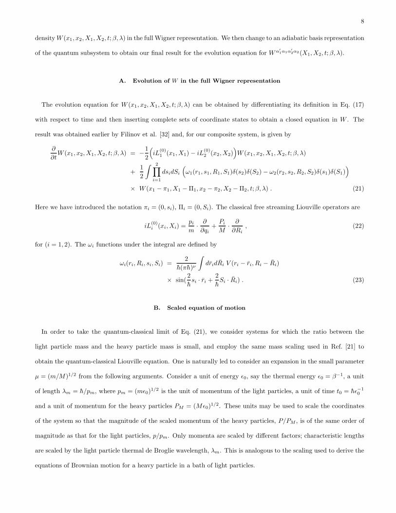
A. Evolution of W in the full Wigner representation

The evolution equation for W (x1, x2, X1, X2, t; β, λ) can be obtained by differentiating its definition in Eq. (17)

with respect to time and then inserting complete sets of coordinate states to obtain a closed equation in W . The

result was obtained earlier by Filinov et al. [32] and, for our composite system, is given by

∂

∂tW (x1, x2, X1, X2, t; β, λ) = −

1

2

(

iL(0)1 (x1, X1) − iL

(0)2 (x2, X2)

)

W (x1, x2, X1, X2, t; β, λ)

+1

2

∫ 2∏

i=1

dsidSi

(

ω1(r1, s1, R1, S1)δ(s2)δ(S2) − ω2(r2, s2, R2, S2)δ(s1)δ(S1))

× W (x1 − π1, X1 − Π1, x2 − π2, X2 − Π2, t; β, λ) . (21)

Here we have introduced the notation πi = (0, si), Πi = (0, Si). The classical free streaming Liouville operators are

iL(0)i (xi, Xi) =

pi

m·

∂

∂qi+

Pi

M·

∂

∂Ri, (22)

for (i = 1, 2). The ωi functions under the integral are defined by

ωi(ri, Ri, si, Si) =2

h(πh)ν

∫

dridRi V (ri − ri, Ri − Ri)

× sin(2

hsi · ri +

2

hSi · Ri) . (23)

B. Scaled equation of motion

In order to take the quantum-classical limit of Eq. (21), we consider systems for which the ratio between the

light particle mass and the heavy particle mass is small, and employ the same mass scaling used in Ref. [21] to

obtain the quantum-classical Liouville equation. One is naturally led to consider an expansion in the small parameter

µ = (m/M)1/2 from the following arguments. Consider a unit of energy ǫ0, say the thermal energy ǫ0 = β−1, a unit

of length λm = h/pm, where pm = (mǫ0)1/2 is the unit of momentum of the light particles, a unit of time t0 = hǫ−1

0

and a unit of momentum for the heavy particles PM = (Mǫ0)1/2. These units may be used to scale the coordinates

of the system so that the magnitude of the scaled momentum of the heavy particles, P/PM , is of the same order of

magnitude as that for the light particles, p/pm. Only momenta are scaled by different factors; characteristic lengths

are scaled by the light particle thermal de Broglie wavelength, λm. This is analogous to the scaling used to derive the

equations of Brownian motion for a heavy particle in a bath of light particles.

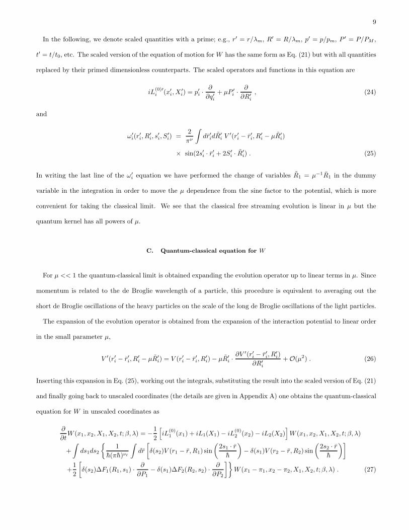
9

In the following, we denote scaled quantities with a prime; e.g., r′ = r/λm, R′ = R/λm, p′ = p/pm, P ′ = P/PM ,

t′ = t/t0, etc. The scaled version of the equation of motion for W has the same form as Eq. (21) but with all quantities

replaced by their primed dimensionless counterparts. The scaled operators and functions in this equation are

iL(0)′i (x′

i, X′i) = p′i ·

∂

∂q′i+ µP ′

i ·∂

∂R′i

, (24)

and

ω′i(r

′i, R

′i, s

′i, S

′i) =

2

πν

∫

dr′idR′i V ′(r′i − r′i, R

′i − µR′

i)

× sin(2s′i · r′i + 2S′

i · R′i) . (25)

In writing the last line of the ω′i equation we have performed the change of variables R1 = µ−1R1 in the dummy

variable in the integration in order to move the µ dependence from the sine factor to the potential, which is more

convenient for taking the classical limit. We see that the classical free streaming evolution is linear in µ but the

quantum kernel has all powers of µ.

C. Quantum-classical equation for W

For µ << 1 the quantum-classical limit is obtained expanding the evolution operator up to linear terms in µ. Since

momentum is related to the de Broglie wavelength of a particle, this procedure is equivalent to averaging out the

short de Broglie oscillations of the heavy particles on the scale of the long de Broglie oscillations of the light particles.

The expansion of the evolution operator is obtained from the expansion of the interaction potential to linear order

in the small parameter µ,

V ′(r′i − r′i, R′i − µR′

i) = V (r′i − r′i, R′i) − µR′

i ·∂V ′(r′i − r′i, R

′i)

∂R′i

+ O(µ2) . (26)

Inserting this expansion in Eq. (25), working out the integrals, substituting the result into the scaled version of Eq. (21)

and finally going back to unscaled coordinates (the details are given in Appendix A) one obtains the quantum-classical

equation for W in unscaled coordinates as

∂

∂tW (x1, x2, X1, X2, t; β, λ) = −

1

2

[

iL(0)1 (x1) + iL1(X1) − iL

(0)2 (x2) − iL2(X2)

]

W (x1, x2, X1, X2, t; β, λ)

+

∫

ds1ds2

{

1

h(πh)νℓ

∫

dr

[

δ(s2)V (r1 − r, R1) sin

(

2s1 · r

h

)

− δ(s1)V (r2 − r, R2) sin

(

2s2 · r

h

)]

+1

2

[

δ(s2)∆F1(R1, s1) ·∂

∂P1− δ(s1)∆F2(R2, s2) ·

∂

∂P2

]}

W (x1 − π1, x2 − π2, X1, X2, t; β, λ) . (27)

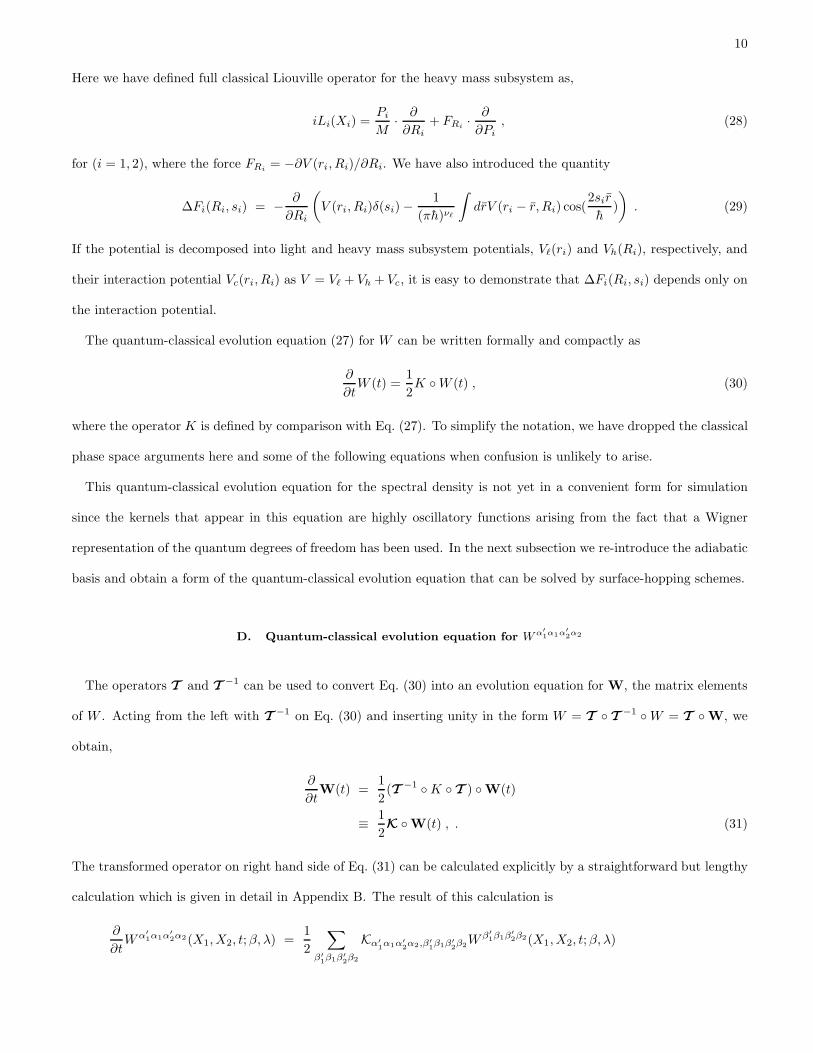
10

Here we have defined full classical Liouville operator for the heavy mass subsystem as,

iLi(Xi) =Pi

M·

∂

∂Ri+ FRi

·∂

∂Pi, (28)

for (i = 1, 2), where the force FRi= −∂V (ri, Ri)/∂Ri. We have also introduced the quantity

∆Fi(Ri, si) = −∂

∂Ri

(

V (ri, Ri)δ(si) −1

(πh)νℓ

∫

drV (ri − r, Ri) cos(2sir

h)

)

. (29)

If the potential is decomposed into light and heavy mass subsystem potentials, Vℓ(ri) and Vh(Ri), respectively, and

their interaction potential Vc(ri, Ri) as V = Vℓ + Vh + Vc, it is easy to demonstrate that ∆Fi(Ri, si) depends only on

the interaction potential.

The quantum-classical evolution equation (27) for W can be written formally and compactly as

∂

∂tW (t) =

1

2K ◦ W (t) , (30)

where the operator K is defined by comparison with Eq. (27). To simplify the notation, we have dropped the classical

phase space arguments here and some of the following equations when confusion is unlikely to arise.

This quantum-classical evolution equation for the spectral density is not yet in a convenient form for simulation

since the kernels that appear in this equation are highly oscillatory functions arising from the fact that a Wigner

representation of the quantum degrees of freedom has been used. In the next subsection we re-introduce the adiabatic

basis and obtain a form of the quantum-classical evolution equation that can be solved by surface-hopping schemes.

D. Quantum-classical evolution equation for Wα′

1α1α′

2α2

The operators T and T−1 can be used to convert Eq. (30) into an evolution equation for W, the matrix elements

of W . Acting from the left with T−1 on Eq. (30) and inserting unity in the form W = T ◦ T

−1 ◦ W = T ◦ W, we

obtain,

∂

∂tW(t) =

1

2(T −1 ◦ K ◦ T ) ◦ W(t)

≡1

2K ◦ W(t) , . (31)

The transformed operator on right hand side of Eq. (31) can be calculated explicitly by a straightforward but lengthy

calculation which is given in detail in Appendix B. The result of this calculation is

∂

∂tWα′

1α1α′

2α2(X1, X2, t; β, λ) =1

2

∑

β′

1β1β′

2β2

Kα′

1α1α′

2α2,β′

1β1β′

2β2

W β′

1β1β′

2β2(X1, X2, t; β, λ)

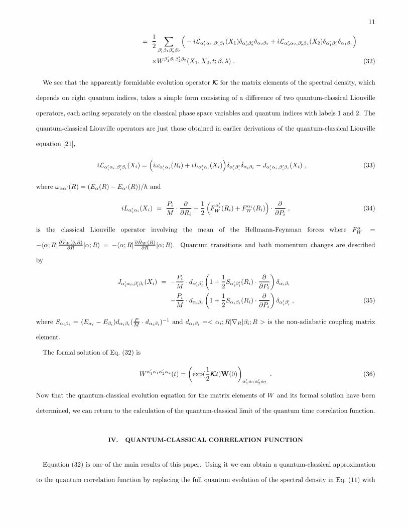
11

=1

2

∑

β′

1β1β′

2β2

(

− iLα′

1α1,β′

1β1(X1)δα′

2β′

2δα2β2 + iLα′

2α2,β′

2β2(X2)δα′

1β′

1δα1β1

)

×W β′

1β1β′

2β2(X1, X2, t; β, λ) . (32)

We see that the apparently formidable evolution operator K for the matrix elements of the spectral density, which

depends on eight quantum indices, takes a simple form consisting of a difference of two quantum-classical Liouville

operators, each acting separately on the classical phase space variables and quantum indices with labels 1 and 2. The

quantum-classical Liouville operators are just those obtained in earlier derivations of the quantum-classical Liouville

equation [21],

iLα′

iαi,β′

iβi

(Xi) =(

iωα′

iαi

(Ri) + iLα′

iαi

(Xi))

δα′

iβ′

iδαiβi

− Jα′

iαi,β′

iβi

(Xi) , (33)

where ωαα′(R) = (Eα(R) − Eα′(R))/h and

iLα′

iαi

(Xi) =Pi

M·

∂

∂Ri+

1

2

(

Fα′

i

W (Ri) + Fαi

W (Ri))

·∂

∂Pi, (34)

is the classical Liouville operator involving the mean of the Hellmann-Feynman forces where FαW =

−〈α; R|∂VW (q,R)∂R |α; R〉 = −〈α; R|∂HW (R)

∂R |α; R〉. Quantum transitions and bath momentum changes are described

by

Jα′

iαi,β′

iβi

(Xi) = −Pi

M· dα′

iβ′

i

(

1 +1

2Sα′

iβ′

i(Ri) ·

∂

∂Pi

)

δαiβi

−Pi

M· dαiβi

(

1 +1

2Sαiβi

(Ri) ·∂

∂Pi

)

δα′

iβ′

i, (35)

where Sαiβi= (Eαi

− Eβi)dαiβi

( PM · dαiβi

)−1 and dαiβi=< αi; R|∇R|βi; R > is the non-adiabatic coupling matrix

element.

The formal solution of Eq. (32) is

Wα′

1α1α′

2α2(t) =

(

exp(1

2Kt)W(0)

)

α′

1α1α′

2α2

. (36)

Now that the quantum-classical evolution equation for the matrix elements of W and its formal solution have been

determined, we can return to the calculation of the quantum-classical limit of the quantum time correlation function.

IV. QUANTUM-CLASSICAL CORRELATION FUNCTION

Equation (32) is one of the main results of this paper. Using it we can obtain a quantum-classical approximation

to the quantum correlation function by replacing the full quantum evolution of the spectral density in Eq. (11) with

12

its evolution in the quantum-classical limit given by Eq. (36), the solution of Eq. (32). We have

CAB(t; β) =1

β

∫ β

0

dλ∑

α1,α′

1,α2,α′

2

∫ 2∏

i=1

dXi B†α1α′

1

W (X1)Aα2α′

2

W (X2)

×(

exp(1

2Kt)W(X1, X2, 0; β, λ)

)

α′

1α1α′

2α2

. (37)

Since the operator K is the sum of two operators, one acting only on functions of X1 and quantum indices with

subscript 1, and the other on functions of X2 and quantum indices with subscript 2, we may integrate by parts to

have the operator act on the dynamical variables instead of W. We obtain,

CAB(t, β) =∑

β′

1β1β′

2β2

∫ 2∏

i=1

dXi B†β1β′

1

W (X1,t

2)A

β2β′

2

W (X2,−t

2)W

β′

1β1β′

2β2(X1, X2; β) , (38)

where

B†β1β′

1

W (X1,t

2) =

∑

α′

1α1

(

ei t2L(X1)

)

β1β′

1α1α′

1

B†α1α′

1

W (X1) ,

Aβ2β′

2

W (X2,−t

2) =

∑

α′

2α2

(

e−i t2L(X2)

)

β2β′

2α2α′

2

Aα2α′

2

W (X2) . (39)

In writing Eq. (38) we defined

Wβ′

1β1β′

2β2(X1, X2; β) =

1

β

∫ β

0

dλ W β′

1β1β′

2β2(X1, X2, 0; β, λ) . (40)

Equation (38) shows that the correlation function at time t can be calculated by sampling X1 and X2 from suitable

weights determined by Wβ′

1β1β′

2β2(X1, X2; β) at time zero and propagating B

†α1α′

1

W forward in time and Aα2α′

2

W backward

in time for an interval of length t/2. Note that while the time evolution in Eq. (38) is by quantum-classical dynamics,

the initial condition for Wβ′

1β1β′

2β2(X1, X2; β) is still an exact expression for the full equilibrium quantum mechanical

spectral density.

V. HIGH TEMPERATURE FORM OF W

At t = 0 W is given explicitly by

Wα′

1α1α′

2α2(X1, X2, 0; β, λ) =1

(2πh)2νhZQ

∫

dZ1dZ2e− i

h(P1Z1+P2Z2)

× 〈α′1; R1|〈R1 +

Z1

2|e−(β−λ)H |R2 −

Z2

2〉|α2; R2〉

× 〈α′2; R2|〈R2 +

Z2

2|e−λH |R1 −

Z1

2〉|α1; R1〉 . (41)

13

It can be computed using path integral techniques but its evaluation is still a difficult problem. In order to illustrate

its structure we consider its form in the high temperature limit. In this limit we may write

〈R2 +Z2

2|e−λH |R1 −

Z1

2〉 ≈ e−λh(Rc−

14 Z12)

(

M

2πλh2

)νh/2

exp

[

−M(R12 − Zc)

2

2λh2

]

, (42)

where h = p2

2m + V and we have introduced the variables Zc = (Z1 + Z2)/2, Z12 = Z1 − Z2, Rc = (R1 + R2)/2 and

R12 = R1 − R2. Taking the desired matrix element of this expression and inserting complete sets of adiabatic states

we obtain

〈α′2; R2|〈R2 +

Z2

2|e−λh|R1 −

Z1

2〉|α1; R1〉 =

∑

α

e−λEα(Rc−Z122 )〈α′

2; R2|α; Rc −Z12

4〉〈α; Rc −

Z12

4|α1; R1〉

=∑

α

e−λEα(Rc)〈α′2; R2|α; Rc〉〈α; Rc|α1; R1〉 + O(Z12) . (43)

Keeping only the zero order term in Z12, the integral over Z12 in Eq. (41) gives a factor (4πh)νhδ(P1 −P2). The other

term in Eq. (41), which arises from the combination of the gaussian on the right hand side of Eq. (42) along with the

analogous expression coming from the high temperature limit of 〈R1 + Z1

2 |e−(β−λ)H |R2 − Z2

2 〉, can be evaluated by

performing the gaussian integral on Zc to obtain

(

M

2πh2β

)νh/2

eih

2Pc2λ−β

βR12e

− 2M

h2(β)R2

12e−λ(β−λ)

β

2P2c

M =

(

M

2πh2β

)νh/2

f(R12, Pc)e−

λ(β−λ)β

2P2c

M , (44)

where Pc = (P1 + P2)/2. The function f(R12, Pc) still contains quantum information since it is composed of a

phase factor and a gaussian expressing quantum dispersion effects in the heavy mass coordinates. We can obtain a

classical bath approximation if we represent f(R12, Pc) in a multipole expansion and keep only the first order term,

f(R12, Pc) ≈ [∫

dR12f(R12, Pc)]δ(R12), we have

f(R12, Pc) ≈

(

πh2β

2M

)νh/2

e−P2

c2βM

(2λ−β)2δ(R12) (45)

Combining terms we obtain a high-temperature, classical-bath approximation to W:

Wα′

1α1α′

2α2(X1, X2, 0; β, λ) ≈1

(2πh)νhZQe−β

P21

2M e−(β−λ)Eα′

1(R1)

e−λEα′

2(R1)

δα′

1α2

δα′

2α;R1

δ(R12)δ(P12) . (46)

Thus the quantity W, defined in Eq. (40), is given in the high-temperature, classical-bath limit by

Wα′

1α1α′

2α2(X1, X2; β) =

1

(2πh)νhZQe−β

(

P21

2M+Eα′

1(R1)

)

eβ(Eα′

1(R1)−Eα′

2(R1))

− 1

β(Eα′

1(R1) − Eα′

2(R1))

× δα′

1α2δα′

2α;R1δ(R12)δ(P12) . (47)

Using similar manipulations, the high temperature limit of ZQ is

ZQ ≈1

(2πh)νh

∑

α

∫

dRdPe−β

(

P2

2M+Eα(R)

)

. (48)

14

If Eq. (47) is used in the correlation function formula, Eq. (38), the result maybe shown to correspond with the

quantum-classical linear response theory form [29] to lowest order in h.

VI. CONCLUSION

The expression for the quantum-classical limit of the quantum correlation function derived in this paper provides a

route for the calculation of quantum transport properties in condensed phase systems. Difficult many-body quantum

dynamics is replaced by quantum-classical evolution which can be carried out using surface-hopping schemes involving

probabilistic sampling of quantum transitions, with associated momentum changes in the bath, and classical trajectory

segments. The classical trajectory segments are accompanied by phase factors that account for quantum coherence

when off-diagonal matrix elements appear. [21] The full equilibrium quantum structure of the entire system is retained.

While the equilibrium calculation is still a difficult problem it is more tractable than the quantum dynamics needed

to treat the many-body system using full quantum dynamics. For example, imaginary time Feynman path integral

methods for computing equilibrium properties are far more tractable than their corresponding real time variants. Since

quantum information about the entire system is retained in the equilibrium structure, the formula for the correlation

function incorporates some aspects of nuclear bath quantum dispersion that is missing in other quantum-classical

schemes. The importance of retaining the full quantum equilibrium structure has been noted in Ref. [33].

The results also provide a framework for exploring and extending the statistical mechanics of quantum-classical

systems. The correlation functions for transport properties that result from linear response theory in quantum-classical

systems involve both quantum-classical evolution like that derived in this paper, as well as the equilibrium quantum-

classical density that is stationary under the quantum-classical evolution. [29, 30] One may construct approximations

to quantum transport properties by considering other approximate limiting forms of the equilibrium spectral density.

We also note that to establish a complete comparison with quantum-classical linear response theory requires the

retention of terms that were neglected in the calculations for W presented in Sec. V. It should be fruitful to pursue

extensions of such calculations to obtain other approximations for quantum transport properties.

Acknowledgements

This work was supported in part by a grant from the Natural Sciences and Engineering Research Council of Canada.

RK would like to thank S. Bonella and G. Ciccotti for discussions pertaining to part of the work presented here.

15

Appendix A: DERIVATION OF QUANTUM-CLASSICAL EVOLUTION EQUATION FOR W

The equation of motion for the spectral density (Eq. (21)) takes a similar form in scaled coordinates:

∂

∂tW ′(x′

1, x′2, X

′1, X

′2, t

′; β′, λ′) = −1

2

(

iL(0)′1 (x′

1, X′1) − iL

(0)′2 (x′

2, X′2)

)

W ′(x′1, x

′2, X

′1, X

′2, t

′; β′, λ′)

+1

2

∫ 2∏

i=1

ds′idS′i

(

ω′1(r

′1, s

′1, R

′1, S

′1)δ(s

′2)δ(S

′2) − ω′

2(r′2, s

′2, R

′2, S

′2)δ(s

′1)δ(S

′1)

)

× W ′(x′1 − π′

1, X′1 − Π′

1, x′2 − π′

2, X′2 − Π′

2, t′; β′, λ′) , (A1)

where the scaled free streaming Liouville operator and integral kernel are defined in Eqs. (24) and (25), respectively.

Inserting Eq. (26) into the expression for ω′1 and retaining only terms up to linear order in in µ we find

ω′1(r

′1, s

′1, R

′1, S

′1) ≈

2

(π)ν

∫

dr′1dR′1V

′(r′1 − r′1, R′1) sin

(

2s′1 · r′1 + 2S′

1 · R′1

)

−2µ

(π)ν

∫

dr′1dR′1

∂V ′(r′1 − r′1, R′1)

∂R′1

· R′1 sin

(

2s′1 · r′1 + 2S′

1 · R′1

)

+ O(µ2) . (A2)

We observe that

∫

dr′1dR′1V

′(r′1 − r′1, R′1) sin

(

2s′1 · r′1 + 2S′

1 · R′1

)

=

∫

dr′1dR′1V

′(r′1 − r′1, R′1)

[

sin(2s′1 · r′1) cos(2S′

1 · R′1)

+ cos(2s′1 · r′1) sin(2S′

1 · R′1)

]

, (A3)

using the trigonometric identity for the sine of a sum of arguments. Then, using the fact that∫

dR′1cos(2S′

1R′1) =

πνhδ(S′1) we have

∫

dr′1dR′1V

′(r′1 − r′1, R′1) sin

(

2s′1 · r′1 + 2S′

1 · R′1

)

= πνh

∫

dr′1V′(r′1 − r′1, R

′1) sin(2s′1 · r

′1)δ(S

′1) , (A4)

where we have used∫

dR′1 sin(2S′

1 · R′1) = 0. In a similar manner

∫

dr′1dR′1

∂V ′(r′1 − r′1, R′1)

∂R′1

· R′1 sin

(

2s′1 · r′1 + 2S′

1 · R′1

)

= −πνh

2

∫

dr′1∂V ′(r′1 − r′1, R

′1)

∂R′1

cos(2s′1 · r′1) ·

dδ(S′1)

dS′1

,

(A5)

where we have used the relations∫

dR′1R

′1 cos(2S′

1 · R′1) = 0 and

∫

dR′1R

′1 sin(2S′

1 · R′1) = −(πνh/2)dδ(S′

1)/dS′1. Then

to order O(µ),

ω′1(r

′1, s

′1, R

′1, S

′1) =

2

πνℓ

∫

dq′V ′(r′1 − r′1, R′1) sin(2s′1 · r

′1)δ(S

′1)

+ µ

[

1

πνℓ

∫

dr′1∂V ′(r′1 − r′1, R

′1)

∂R′1

cos(2s′1 · r′1) ·

dδ(S′1)

dS′1

]

. (A6)

Using this expression we may compute the integral on the right hand side of Eq. (A1) involving ω′1. The algebra

for the ω′2 term is similar. Given the expression (A6), the integral

∫

ds′1dS′1ω

′1(r

′1, s

′1, R

′1, S

′1)W

′(x′1 − π′

1, X′1 − Π′

1, x′2, X

′2, t

′; β, λ) , (A7)

16

has two contributions. The first is is

2

πνℓ

∫

ds′1dS′1W

′(x′1 − π′

1, X′1 − Π′

1, x′2, X

′2, t

′; β, λ)

∫

dr′1V′(r′1 − r′1, R

′1) sin(2s′1 · r

′1)δ(S

′1) =

2

πνℓ

∫

ds′1W′(x′

1 − π′1, X

′1, x

′2, X

′2; t

′, β, λ)

∫

dr′1V′(r′1 − r′1, R

′1) sin(2s′1 · r

′1) , (A8)

while the second is

µ

πνℓ

∫

ds′1dS′1W

′(x1 − π′1, X

′1 − Π′

1, x′2, X

′2, t

′; β, λ)

∫

dr′1∂

∂R′1

V ′(r′1 − r′1, R′1) cos(2s′1 · r

′1) ·

dδ(S′1)

dS′1

=

µ

πνℓ

∫

ds′1∂

∂P ′1

W ′(x′1 − π′

1, X′1, x

′2, X

′2, t

′; β, λ) ·

∫

dr′1∂

∂R′1

V ′(r′1 − r′1, R′1) cos(2s′1 · r

′1) . (A9)

Defining ∆F ′R′

1,s′

1= − ∂

∂R′

1

[

V ′(R′1)δ(s

′1) −

1πνℓ

∫

dr′1 cos(2s′1 · r′1)V

′(r′1 − r′1, R′1)

]

and returning to unscaled coordinates

we obtain Eq. (27), the desired quantum-classical evolution equation for the full Wigner representation of W . The

first term in the definition of ∆F ′ is compensated by the introduction of the full classical propagator for the heavy

mass degrees of freedom. Written in this form, ∆F ′ also depends only on the interaction potential between the light

and heavy mass particles.

Appendix B: EQUATION IN THE PARTIAL WIGNER REPRESENTATION

In this appendix we perform explicitly the calculations that, starting from Eq. (27), lead to Eq. (32). This calculation

amounts to the evaluation of (T −1 ◦ K ◦ T ) ◦ W(t). The various terms in K, defined by Eq. (27), are considered

separately.

Consider the calculation of (T −1 ◦ iL1(X1) ◦ T ) ◦ W which is composed of two terms. The force term is T −1 ◦

FR1 · ∂/∂P1T ◦ W = FR1 · ∂/∂P1W, since T and its inverse do not depend on P1. The free streaming term

(T −1 ◦ P1

M · ∂∂R1

◦ T ) ◦W requires additional calculations since T depends on R1. We have

(T −1 ◦P1

M·

∂

∂R1◦ T ) ◦ W =

P1

M·

∑

β1β′

1β2β′

2

∫ 2∏

j=1

drjdzjφ∗α′

1(r1 +

z1

2, R1)φα1 (r1 −

z1

2, R1)

× φ∗α′

2(q2 +

z2

2; R2)φα2(r2 −

z2

2; R2)φβ′

2(r2 +

z2

2; R2)φ

∗β2

(q2 −z2

2; R2)

×

{[

∂φβ′

1(r1 + z1

2 ; R1)

∂R1φ∗

β1(r1 −

z1

2; R1) + φβ′

1(r1 +

z1

2; R1)

∂φ∗β1

(r1 −z1

2 ; R1)

∂R1

]

W β′

1β1β′

2β2

+ φβ′

1(r1 +

z1

2; R1)φ

∗β1

(r1 −z1

2; R1)

∂

∂R1W β′

1β1β′

2β2

}

. (B1)

The last term where ∂W/∂R1 appears is simple to calculate and gives P1

M · ∂∂R1

Wα′

1α1α′

2α2 . To calculate the other

two terms, we make the change of variables q1 = r1 −z1

2 , q2 = r1 + z1

2 , q3 = r2 −z2

2 , q4 = r2 + z2

2 . Integrating over

17

q3 and q4 and using∫

dqφα(q, R)φ∗β(q, R) = δαβ, we obtain

P1

M·∑

β1β′

1

∫

dq1dq2φ∗α′

1(q2; R1)φα1(q1; R1)

[

∂φβ′

1(q2; R1)

∂R1φ∗

β1(q1; R1) + φβ′

1(q2; R1)

∂φ∗β1

(q1; R1)

∂R1

]

W β′

1β1α′

2α2

=P1

M·∑

β′

1

dα′

1β′

1W β′

1α1α′

2α2 −P1

M·∑

β1

dβ1α1Wα′

1β1α′

2α2 , (B2)

where we have introduced the definition of the nonadiabatic coupling vector.

Consider the calculation of (T −1 ◦ iL(0)1 (x1)◦T )◦W. In this case one integration over the momentum, arising from

the definition of T −1, gives∫

dp1(p1/m)eih

p1(z1−z3) = (2πh)νℓ(ih/m)∂δ(z1 − z3)/∂z3, while integration over p2 gives

(2πh)νℓδ(z2 − z4). One can then integrate by parts on z3 and obtain

(T −1 ◦p1

m

∂

∂r1◦ T ) ◦ W = −

ih

m

∑

β1β′

1β2β′

2

∫ 2∏

j=1

drj

3∏

k=1

dzkδ(z1 − z3)φ∗α′

1(r1 +

z1

2; R1)φα1 (r1 −

z1

2; R1)

×φ∗α′

2(r2 +

z2

2; R2)φα2(r2 −

z2

2; R2)φβ′

2(r2 +

z2

2; R2)φ

∗β2

(r2 −z2

2; R2)

×∂2

∂z3∂r1

[

φβ′

1(r1 +

z3

2; R1)φ

∗β1

(r1 −z3

2; R1)

]

W β′

1β1β′

2β2 . (B3)

Then use

∂2

∂z3∂r1

[

φβ′

1(r1 +

z3

2; R1)φ

∗β1

(r1 −z3

2; R1)

]

=1

2

[

∂2φβ′

1(r1 + z3

2 ; R1)

∂(r1 + z3

2 )2φ∗

β1(r1 −

z3

2; R1) − φβ′

1(r1 +

z3

2; R1)

∂2φ∗β1

(r1 −z3

2 ; R1)

∂(r1 −z3

2 )2

]

, (B4)

go back to the integral, perform the integration on z3 and make the change of variables previously introduced. The

integration over q3 and q4 can be performed using the completeness of the adiabatic basis and one gets

(T −1 ◦p1

m

∂

∂r1◦ T ) ◦ W =

i

h

∑

β′

1

〈α′1; R1|

p2

2m|β′

1; R1〉Wβ′

1α1α′

2α2

−i

h

∑

β1

〈β1; R1|p2

2m|α1; R1〉W

α′

1β1α′

2α2 , (B5)

where we have used the identity 〈α, R|p2/2m|β, R〉 = −(h2/2m)∫

dqφ∗α(q, R)∂φβ(q, R)/∂q2.

We consider now the transformation of the potential term in K ◦ W equal to c1

∫

ds1ds2δ(s2)∫

drV (r1 −

r) sin(

2s1·rh

)

W (x1 − π1, x2 − π2, X1, X2, t; βλ), where c1 = 2h−1(πh)−νℓ ; we may immediately perform the trivial

integrations on p1, p2, z3 and z4. We also make the change variables below Eq. (B1) so that the integrations on q3

and q4 are also trivial. One is left with the integral

c1

∑

β′

1β1

∫

dq1dq2

∫

ds1drV (q1 + q2

2− r) sin

(

2s1 · r

h

)

eih

s1·(q2−q1)

×φ∗α′

1(q2; R1)φα1(q1; R1)φβ′

1(q2; R1)φ

∗β1

(q1; R1)Wβ′

1β1α′

2α2 . (B6)

18

Using the fact that∫

ds1eih

s1·(q2−q1) sin (2s1 · r/h) = (2πh)νℓ [δ(q2 − q1 + 2r) − δ(q2 − q1 − 2r)] /2i, substituting into

Eq. (B6) and making the change of variable σ = 2r, the delta functions can be integrated out and one obtains,

1

ih

∑

β′

1β1

[∫

dq1φα1 (q1; R1)φ∗β1

(q1; R1)

] [∫

dq2φ∗α′

1(q2; R1)V (q2)φβ′

1(q2; R1)

]

W β′

1β1α′

2α2

−1

ih

∑

β′

1β1

[∫

dq1φ∗β1

(q1; R1)V (q1)φα1 (q1; R1)

] [∫

dq2φ∗α′

1(q2; R1)φβ′

1(q2; R1)

]

W β′

1β1α′

2α2

=1

ih

∑

β′

1

〈α′1; R1|V |β′

1; R1〉Wβ′

1α1α′

2α2 −1

ih

∑

β1

〈β1; R1|V |α1; R1〉Wα′

1β1α′

2α2 . (B7)

The last term that must be worked out explicitly arises from the transformation of the quantum-classical term

∫

ds1ds2δ(s2)∆F1(R1, s1) ·∂

∂P1W (x1 − π1, x2 − π2, X1, X2, t; λ, β). Recalling the expression for ∆F1 in Eq. (29) one

sees that there are two contributions to transform. The transformation of the term involving ∂V (R1)∂R1

δ(s1) is the same

as that for the force term in iL1(X1) and yields FR1 · ∂Wα′

1α1α′

2α2/∂P1. The integral term in ∆F1(R1, s1) can be

computed by integrating over p1, p2, z3 and z4, performing the change of variables below Eq. (B1) and integrating

over q3 and q4, to obtain

∑

β′

1β1

1

(πh)νℓ

∫

dq1dq2φ∗α′

1(q2; R1)φα1(q1; R1)φβ′

1(q2; R1)φ

∗β1

(q1; R1)

×

∫

ds1

∫

dr

(

∂

∂R1V (

q1 + q2

2− r, R1)

)

cos

(

2s1 · r

h

)

eih

s1·(q2−q1) ∂

∂P1W β′

1β1α′

2α2 . (B8)

Then one can use the integral∫

ds1 cos (2s1 · r/h) eih

s1·(q2−q1) = (2πh)νℓ [δ(q2 − q1 + 2r) + δ(q2 − q1 − 2r)] /2, make

the change of variable σ = 2r, and integrate out the delta functions to find

1

2

∑

β′

1

〈α′1; R1|

∂V (R1)

∂R1|β′

1; R1〉∂

∂P1W β′

1α1α′

2α2 +∑

β1

〈β1; R1|∂V (R1)

∂R1|α1; R1〉

∂

∂P1Wα′

1β1α′

2α2

. (B9)

Analogous terms (but with opposite sign) are obtained when considering the transformation of the terms depending

on x2 and X2 in Eq. (27).

Combining all terms and using the relations FαβW (R) = −〈α; R|∇RV (R)|β; R〉 = Fα

W + (Eα − Eβ)dαβ ,

−i

h

∑

β′

1

〈α′1; R1|

(

p2

2m+ V

)

|β′1; R1〉W

β′

1α1α′

2α2 +i

h

∑

β1

〈β1; R1|

(

p2

2m+ V

)

|α1; R1〉Wα′

1β1α′

2α2 =

= −i

h(Eα′

1(R1) − Eα1(R1))W

α′

1α1α′

2α2 = −iωα′

1α1

(R1)Wα′

1α1α′

2α2 , (B10)

and introducing the definition Sαiβi= (Eαi

− Eβi)dαiβi

( PM · dαiβi

)−1, we find Eq. (32).

[1] R. Kubo: J. Phys. Soc. (Japan) 12, 570 (1957); R. Kubo: Repts. Prog. Phys. 29, 255 (1966).

19

[2] H. Mori, Prog. Theor. Phys. 33, 423 (1965).

[3] E. Rabani and D. Reichman, J. Chem. Phys. 120, 1458 (2004).

[4] S. A. Egorov, E. Rabani and B. J. Berne, J. Phys. Chem. B 103, 10978 (1999).

[5] A. A. Golosov, D. R. Reichman and E. Rabani, J. Chem. Phys. 118, 457 (2003).

[6] P. Pechukas, Phys. Rev. 181, 166, 174 (1969).

[7] M. F. Herman, Annu. Rev. Phys. Chem. 45, 83 (1994).

[8] J. C. Tully, Modern Methods for Multidimensional Dynamics Computations in Chemistry, ed. D. L. Thompson, (World

Scientific, NY, 1998), p. 34.

[9] J.C. Tully, J. Chem. Phys. 93, 1061 (1990); J.C. Tully: Int. J. Quantum Chem. 25, 299 (1991); S. Hammes-Schiffer and

J.C. Tully: J. Chem. Phys. 101, 4657 (1994); D. S. Sholl and J. C. Tully, J. Chem. Phys. 109, 7702 (1998).

[10] L. Xiao and D. F. Coker, J. Chem. Phys. 100, 8646 (1994); D. F. Coker and L. Xiao: J. Chem. Phys. 102, 496 (1995);

H. S. Mei and D.F. Coker: J. Chem. Phys. 104, 4755 (1996).

[11] F. Webster, P. J. Rossky, and P. A. Friesner, Comp. Phys. Comm. 63, 494 (1991); F. Webster, E. T. Wang, P. J. Rossky,

and P. A. Friesner: J. Chem. Phys. 100, 483 (1994).

[12] T. J. Martinez, M. Ben-Nun, and R. D. Levine, J. Phys. Chem. A 101, 6389 (1997).

[13] A. Warshel and Z. T. Chu, J. Chem. Phys. 93 4003 (1990).

[14] I. V. Aleksandrov, Z. Naturforsch. 36a, 902 (1981).

[15] V. I. Gerasimenko, Repts. Ukranian Acad. Sci. 10, 65 (1981); Teo. Mat. Fiz. 150, 7 (1982).

[16] W. Boucher and J. Traschen, Phys. Rev. D 37, 3522 (1988).

[17] W. Y. Zhang and R. Balescu, J. Plasma Phys. 40, 199 (1988); R. Balescu and W. Y. Zhang, J. Plasma Phys. 40, 215

(1988).

[18] C. C. Martens and J.-Y. Fang, J. Chem. Phys. 106, 4918 (1996); A. Donoso and C. C. Martens, J. Phys. Chem. 102, 4291

(1998); D. Kohen and C. C. Martens, J. Chem. Phys. 111, 4343 (1999); 112, 7345 (2000).

[19] I. Horenko, C. Salzmann, B. Schmidt and C. Schutte, J. Chem. Phys. 117, 11075 (2002).

[20] C. Wan and J. Schofield: J. Chem. Phys. 113, 7047 (2000).

[21] R. Kapral and G. Ciccotti, J. Chem. Phys. 110, 8919 (1999).

[22] E. P. Wigner, Phys. Rev. 40, 749 (1932); K. Imre, E. Ozizmir, M. Rosenbaum and P. F. Zwiefel, J. Math. Phys. 5, 1097

(1967); M. Hillery, R. F. O’Connell, M. O. Scully and E. P. Wigner, Phys. Repts. 106, 121 (1984).

[23] K. Thompson and N. Makri, J. Chem. Phys. 110, 1343 (1999).

[24] D. Mac Kernan, G. Ciccotti and R. Kapral, J. Chem. Phys. 106, (2002).

[25] D. Mac Kernan, G. Ciccotti and R. Kapral, J. Phys. Condens. Matt. 14 9069 (2002).

[26] S. Nielsen, R. Kapral and G. Ciccotti, J. Chem. Phys. 112, 6543 (2000).

20

[27] S. Nielsen, R. Kapral and G. Ciccotti, J. Stat. Phys. 101, 225 (2000).

[28] A. Sergi, D. Mac Kernan, G. Ciccotti and R. Kapral, Theor. Chem. Acc. 110 49 (2003).

[29] S. Nielsen, R. Kapral and G. Ciccotti, J. Chem. Phys. 115, 5805 (2001).

[30] R. Kapral and G. Ciccotti, A Statistical Mechanical Theory of Quantum Dynamics in Classical Environments, in Bridging

Time Scales: Molecular Simulations for the Next Decade, 2001, eds. P. Nielaba, M. Mareschal and G. Ciccotti, (Springer,

Berlin, 2003), p. 445.

[31] A. Sergi and R. Kapral, J. Chem. Phys., 118, 8566 (2003); J. Chem. Phys. 119 12776 (2003).

[32] V. S. Filinov, Y. V. Medvedev and V. L. Kamskyi, Mol. Phys. 85 711 (1995); V. S. Filinov, Mol. Phys. 88 1517 (1996);

V. S. Filinov, Mol. Phys. 88 1529 (1996); V. S. Filinov, S. Bonella, Y. E. Lozovik, A. Filinov and I. Zacharov in Classical

and Quantum Dynamics in Condensed Phase Simulations, edited by B. J. Berne, G. Ciccotti and D. F. Coker (World

Scientific, Singapore, 1998), p. 667.

[33] S. A. Egorov, E. Rabani and B. J. Berne, J. Chem. Phys. 110, 5238 (1999).