arX

iv:q

uant

-ph/

0011

020v

2 1

2 M

ar 2

001

Characteristics of Quantum-Classical Correspondence for Two Interacting Spins

J. Emerson and L.E. BallentinePhysics Department, Simon Fraser University, Burnaby, British Columbia, Canada V5A 1S6

(February 1, 2008)

The conditions of quantum-classical correspondence for a system of two interacting spins areinvestigated. Differences between quantum expectation values and classical Liouville averages areexamined for both regular and chaotic dynamics well beyond the short-time regime of narrow states.We find that quantum-classical differences initially grow exponentially with a characteristic exponentconsistently larger than the largest Lyapunov exponent. We provide numerical evidence that thetime of the break between the quantum and classical predictions scales as log(J /h̄), where J isa characteristic system action. However, this log break-time rule applies only while the quantum-classical deviations are smaller than O(h̄). We find that the quantum observables remain wellapproximated by classical Liouville averages over long times even for the chaotic motions of afew degree-of-freedom system. To obtain this correspondence it is not necessary to introduce thedecoherence effects of a many degree-of-freedom environment.

0.365.Sq,05.45.MT,03.65.Bz

I. INTRODUCTION

There is considerable interest in the interface between quantum and classical mechanics and the conditions thatlead to the emergence of classical behaviour. In order to characterize these conditions, it is important to differentiatetwo distinct regimes of quantum-classical correspondence [1]:(i) Ehrenfest correspondence, in which the centroid of the wave packet approximately follows a classical trajectory.(ii) Liouville correspondence, in which the quantum probability distributions are in approximate agreement with thoseof an appropriately constructed classical ensemble satisfying Liouville’s equation.

Regime (i) is relevant only when the width of the quantum state is small compared to the dimensions of the system;if the initial state is not narrow, this regime may be absent. Regime (ii), which generally includes (i), applies to amuch broader class of states, and this regime of correspondence may persist well after the Ehrenfest correspondencehas broken down. The distinction between regimes (i) and (ii) has not always been made clear in the literature,though the conditions that delimit these two regimes, and in particular their scaling with system parameters, may bequite different.

The theoretical study of quantum chaos has raised the question of whether the quantum-classical break occursdifferently in chaotic states, in states of regular motion, and in mixed phase-space systems. This is well understoodonly in the case of regime (i). There it is well-known [2–4] that the time for a minimum-uncertainty wave packet toexpand beyond the Ehrenfest regime scales as log(J /h̄) for chaotic states, and as a power of J /h̄ for regular states,where J denotes a characteristic system action.

The breakdown of quantum-classical correspondence, in the case of regime (ii), is less well understood, thoughit has been argued that this regime may also be delimited by a log(J /h̄) break-time in classically chaotic states[5,6]. Some numerical evidence in support of this conjecture has been reported in a study of the kicked rotor in theanomolous diffusion regime [7]. (On the other hand, in the regime of quantum localization, the break-time for thekicked rotor seems to scale as (J /h̄)2 [8].) Since the log(J /h̄) time scale is rather short, it has been suggested thatcertain macroscopic objects would be predicted to exhibit non-classical behaviour on observable time scales [9,10].These results highlight the importance of investigating the characteristics of quantum-classical correspondence in moredetail.

In this paper we study the classical and quantum dynamics of two interacting spins. This model is convenientbecause the Hilbert space of the quantum system is finite-dimensional, and hence tractable for computations. Spinmodels have been useful in the past for exploring classical and quantum chaos [3,11–15] and our model belongs toa class of spin models which show promise of experimental realization in the near future [16]. The classical limit isapproached by taking the magnitude of both spins to be very large relative to h̄, while keeping their ratio fixed. Forour model a characteristic system action is given by J ≃ h̄l, where l is a quantum number, and the classical limit issimply the limit of large quantum numbers, i.e. the limit l → ∞.

In the case of the chaotic dynamics for our model, we first show that the widths of both the quantum and classicalstates grow exponentially at a rate given approximately by the largest Lyapunov exponent (until saturation at thesystem dimension). We then show that the initially small quantum-classical differences also grow at an exponential

1

rate, with an exponent λqc that is independent of the quantum numbers and at least twice as large as the largestLyapunov exponent. We demonstrate how this exponential growth of differences leads to a log break-time rule,tb ≃ λ−1

qc ln(lp/h̄), delimiting the regime of Liouville correspondence. The factor p, measured in units of h̄, is somepreset tolerance that defines a break between the quantum and classical expectation values. However, we also showthat this logarithmic rule holds only if the tolerance p for quantum-classical differences is chosen extremely small, inparticular p < O(h̄). For larger values of the tolerance, the break-time does not occur on this log time-scale and maynot occur until the recurrence time. In this sense, log break-time rules describing Liouville correspondence are notrobust. These results demonstrate that, for chaotic states in the classical limit, quantum observables are describedapproximately by Liouville ensemble averages well beyond the Ehrenfest time-scale, after which both quantum andclassical states have relaxed towards equilibrium distributions. This demonstration of correspondence is obtained fora few degree-of-freedom quantum system of coupled spins that is described by a pure state and subject only to unitaryevolution.

This paper is organised as follows. In section II we describe the quantum and classical versions of our model.Since the model is novel we examine the behaviours of the classical dynamics in some detail. In section III we definethe initial quantum states, which are SU(2) coherent states, and then define a corresponding classical density onthe 2-sphere which is a good analog for these states. We show in the Appendix that a perfect match is impossible:no distribution on S2 can reproduce the moments of the SU(2) coherent states exactly. In section IV we describeour numerical techniques. In section V we examine the quantum dynamics in regimes of classically chaotic andregular behaviour and demonstrate the close quantitative correspondence with the Liouville dynamics that persistswell after the Ehrenfest break-time. In section VI we characterize the growth of quantum-classical differences in thetime-domain. In section VII we characterize the scaling of the break-time for small quantum-classical differences andalso examine the scaling of the maximum quantum-classical differences in the classical limit.

II. THE MODEL

We consider the quantum and classical dynamics generated by a non-integrable model of two interacting spins,

H = a(Sz + Lz) + cSxLx

∞∑

n=−∞

δ(t− n) (1)

where S = (Sx, Sy, Sz) and L = (Lx, Ly, Lz). The first two terms in (1) correspond to simple rotation of both spinsabout the z-axis. The sum over coupling terms describes an infinite sequence of δ-function interactions at times t = nfor integer n. Each interaction term corresponds to an impulsive rotation of each spin about the x-axis by an angleproportional to the x-component of the other spin.

A. The Quantum Dynamics

To obtain the quantum dynamics we interpret the Cartesian components of the spins as operators satisfying theusual angular momentum commutation relations,

[Si, Sj ] = iǫijkSk

[Li, Lj] = iǫijkLk

[Ji, Jj ] = iǫijkJk.

In the above we have set h̄ = 1 and introduced the total angular momentum vector J = S + L.The Hamiltonian (1) possesses kinematic constants of the motion, [S2, H ] = 0 and [L2, H ] = 0, and the total state

vector |ψ〉 can be represented in a finite Hilbert space of dimension (2s+ 1)× (2l+ 1). This space is spanned by theorthonormal vectors |s,ms〉 ⊗ |l,ml〉 where ms ∈ {s, s − 1, . . . ,−s} and ml ∈ {l, l − 1, . . . ,−l}. These are the jointeigenvectors of the four spin operators

S2|s, l,ms,ml〉 = s(s+ 1)|s, l,ms,ml〉

Sz|s, l,ms,ml〉 = ms|s, l,ms,ml〉 (2)

L2|s, l,ms,ml〉 = l(l + 1)|s, l,ms,ml〉

Lz|s, l,ms,ml〉 = ml|s, l,ms,ml〉.

2

The periodic sequence of interactions introduced by the δ-function produces a quantum mapping. The time-evolution for a single iteration, from just before a kick to just before the next, is produced by the unitary transfor-mation,

|ψ(n+ 1)〉 = F |ψ(n)〉, (3)

where F is the single-step Floquet operator,

F = exp [−ia(Sz + Lz)] exp [−icSxLx] . (4)

Since a is a rotation its range is 2π radians. The quantum dynamics are thus specified by two parameters, a and c,and two quantum numbers, s and l.

An explicit representation of the single-step Floquet operator can be obtained in the basis (2) by first re-expressingthe interaction operator in (4) in terms of rotation operators,

exp [−icSx ⊗ Lx] = [R(s)(θ, φ) ⊗R(l)(θ, φ)] exp [−icSz ⊗ Lz]

×[R(s)(θ, φ) ⊗R(l)(θ, φ)]−1, (5)

using polar angle θ = π/2 and azimuthal angle φ = 0. Then the only non-diagonal terms arise in the expressions forthe rotation matrices, which take the form,

〈j,m′|R(j)(θ, φ)|j,m〉 = exp(−im′φ)d(j)m′,m(θ). (6)

The matrix elements,

d(j)m′,m(θ) = 〈j,m′| exp(−iθJy)|j,m〉 (7)

are given explicitly by Wigner’s formula [19].We are interested in studying the different time-domain characteristics of quantum observables when the cor-

responding classical system exhibits either regular or chaotic dynamics. In order to compare quantum systemswith different quantum numbers it is convenient to normalize subsystem observables by the subsystem magnitude√

〈L2〉 =√

l(l + 1). We denote such normalized observables with a tilde, where

〈L̃z(n)〉 =〈ψ(n)|Lz |ψ(n)〉

√

l(l+ 1)(8)

and the normalized variance at time n is defined as,

∆L̃2(n) =〈L2〉 − 〈L(n)〉2

l(l+ 1). (9)

We are also interested in evaluating the properties of the quantum probability distributions. The probabilitydistribution corresponding to the observable Lz is given by the trace,

Pz(ml) = Tr[

ρ(l)(n)|l,ml〉〈l,ml|]

= 〈l,ml|ρ(l)(n)|l,ml〉, (10)

where ρ(l)(n) = Tr(s) [ |ψ(n)〉〈ψ(n)| |s,ms〉〈s,ms| ] is the reduced state operator for the spin L at time n and Tr(s)

denotes a trace over the factor space corresponding to the spin S.

B. Classical Map

For the Hamiltonian (1) the corresponding classical equations of motion are obtained by interpreting the angularmomentum components as dynamical variables satisfying,

{Si, Sj} = ǫijkSk

{Li, Lj} = ǫijkLk

{Ji, Jj} = ǫijkJk,

3

with {·, ·} denoting the Poisson bracket. The periodic δ-function in the coupling term can be used to define surfacesat t = n, for integer n, on which the time-evolution reduces to a stroboscopic mapping,

S̃n+1x = S̃n

x cos(a) −[

S̃ny cos(γrL̃n

x) − S̃nz sin(γrL̃n

x)]

sin(a),

S̃n+1y =

[

S̃ny cos(γrL̃n

x) − S̃nz sin(γrL̃n

x)]

cos(a) + S̃nx sin(a),

S̃n+1z = S̃n

z cos(γrL̃nx) + S̃n

y sin(γrL̃nx), (11)

L̃n+1x = L̃n

x cos(a) −[

L̃ny cos(γS̃n

x ) − L̃nz sin(γS̃n

x )]

sin(a),

L̃n+1y =

[

L̃ny cos(γS̃n

x ) − L̃nz sin(γS̃n

x )]

cos(a) + L̃nx sin(a),

L̃n+1z = L̃n

z cos(γS̃nx ) + L̃n

y sin(γS̃nx ),

where L̃ = L/|L| , S̃ = S/|S| and we have introduced the parameters γ = c|S| and r = |L|/|S|. The mappingequations (11) describe the time-evolution of (1) from just before one kick to just before the next.

Since the magnitudes of both spins are conserved, {S2, H} = {L2, H} = 0, the motion is actually confined to thefour-dimensional manifold P = S2 ×S2, which corresponds to the surfaces of two spheres. This is manifest when themapping (11) is expressed in terms of the four canonical coordinates x = (Sz , φs, Lz, φl), where φs = tan(Sy/Sx) andφl = tan(Ly/Lx). We will refer to the mapping (11) in canonical form using the shorthand notation xn+1 = F(xn).

It is also useful to introduce a complete set of spherical coordinates ~θ = (θs, φs, θl, φl) where θs = cos−1(Sz/|S|) andθl = cos−1(Lz/|L|).

The classical flow (11) on the reduced surface P still has a rather large parameter space; the dynamics are determinedfrom three independent dimensionless parameters: a ∈ [0, 2π), γ ∈ (−∞,∞), and r ≥ 1. The first of these, a, controlsthe angle of free-field rotation about the z-axis. The parameter γ = c|S| is a dimensionless coupling strength andr = |L|/|S| corresponds to the relative magnitude of the two spins.

We are particularly interested in the effect of increasing the coupling strength γ for different fixed values of r. InFig. 1 we plot the dependence of the classical behaviour on these two parameters for the case a = 5, which producestypical results. The data in this figure was generated by randomly sampling initial conditions on P , using the canonicalmeasure,

dµ(x) = dS̃zdφsdL̃zdφl, (12)

and then calculating the largest Lyapunov exponent associated with each trajectory. Open circles correspond toregimes where at least 99% of the initial conditions were found to exhibit regular behaviour and crosses correspondto regimes where at least 99% of these randomly sampled initial conditions were found to exhibit chaotic behaviour.Circles with crosses through them (the superposition of both symbols) correspond to regimes with a mixed phasespace. For the case a = 5 and with r held constant, the scaled coupling strength γ plays the role of a perturbationparameter: the classical behaviour varies from regular, to mixed, to predominantly chaotic as |γ| is increased fromzero.

The fixed points of the classical map (11) provide useful information about the parameter dependence of the classicalbehaviour and, more importantly, in the case of mixed regimes, help locate the zones of regular behaviour in the 4-dimensional phase space. We find it sufficient to consider only the four trivial (parameter-independent) fixed pointswhich lie at the poles along the z-axis: two of these points correspond to parallel spins, (Sz, Lz) = ±(|S|, |L|), andthe remaining two points correspond to anti-parallel spins, (Sz, Lz) = (±|S|,∓|L|).

The stability around these fixed points can be determined from the eigenvalues of the tangent map matrix, M =∂F/∂x, where all derivatives are evaluated at the fixed point of interest. (It is easiest to derive M using the six non-

canonical mapping equations (11) since the tangent map for the canonical mapping equations exhibits a coordinatesystem singularity at these fixed points.) The eigenvalues corresponding to the four trivial fixed points are obtainedfrom the characteristic equation,

[ξ2 − 2ξ cos a+ 1]2 ± ξ2γ2r sin2 a = 0, (13)

with the minus (plus) sign corresponding to the parallel (anti-parallel) cases and we have suppressed the trivial factor(1 − ξ)2 which arises since the six equations (11) are not independent. For the parallel fixed points we have the foureigenvalues,

ξP1,2 = cos a±

1

2

√

rγ2 sin2 a+1

2

√

±4 cosa

√

γ2r sin2 a− sin2 a(4 − γ2r),

4

ξP3,4 = cos a±

1

2

√

rγ2 sin2 a−1

2

√

±4 cosa

√

γ2r sin2 a− sin2 a(4 − γ2r), (14)

and the eigenvalues for the anti-parallel cases, ξAP , are obtained from (14) through the substitution r → −r. A fixedpoint becomes unstable if and only if |ξ| > 1 for at least one of the four eigenvalues.

1. Mixed Phase Space: γ = 1.215

We are particularly interested in the behaviour of this model when the two spins are comparable in magnitude.Choosing the value r = 1.1 (with a = 5 as before), we determined by numerical evaluation that the anti-parallelfixed points are unstable for |γ| > 0. In the case of the parallel fixed points, all four eigenvalues remain on the unitcircle, |ξP | = 1, for |γ| < 1.42. This stability condition guarantees the presence of regular islands about the parallelfixed points [20]. In Fig. 2 we plot the trajectory corresponding to the parameters a = 5, r = 1.1, γ = 1.215 and

with initial condition ~θ(0) = (5o, 5o, 5o, 5o) which locates the trajectory near a stable fixed point of a mixed phasespace (see Fig. 1.) This trajectory clearly exhibits a periodic pattern which we have confirmed to be regular bycomputing the associated Lyapunov exponent (λL = 0). In contrast, the trajectory plotted in Fig. 3 is launched with

the same parameters but with initial condition ~θ(0) = (20o, 40o, 160o, 130o), which is close to one of the unstable anti-parallel fixed points. This trajectory explores a much larger portion of the surface of the two spheres in a seeminglyrandom manner. As expected, a computation of the largest associated Lyapunov exponent yields a positive number(λL = 0.04).

2. Global Chaos: γ = 2.835

If we increase the coupling strength to the value γ = 2.835, with a = 5 and r = 1.1 as before, then all four trivialfixed points become unstable. By randomly sampling P with 3 × 104 initial conditions we find that less than 0.1%of the kinematically accessible surface P is covered with regular islands (see Fig. 1). This set of parameters producesa connected chaotic zone with largest Lyapunov exponent λL = 0.45. We will refer to this type of regime as one of‘global chaos’ although the reader should note that our usage of this expression differs slightly from that in [20].

3. The Limit r ≫ 1

Another interesting limit of our model arises when one of the spins is much larger than the other, r ≫ 1. Weexpect that in this limit the larger spin (L) will act as a source of essentially external ‘driving’ for the smaller spin(S). Referring to the coupling terms in the mapping (11), the ‘driving’ strength, or perturbation upon S from L, isdetermined from the product γr = c|L|, which can be quite large, whereas the ‘back-reaction’ strength, or perturbationupon L from S, is governed only by the scaled coupling strength γ = c|S|, which can be quite small. It is interestingto examine whether a dynamical regime exists where the larger system might approach regular behaviour while thesmaller ‘driven’ system is still subject to chaotic motion.

In Fig. 4 we plot a chaotic trajectory for r = 100 with initial condition ~θ(0) = (27o, 27o, 27o, 27o) which is locatedin a chaotic zone (λL = 0.026) of a mixed phase space (with a = 5 and γ = 0.06). Although the small spin wanderschaotically over a large portion of its kinematically accessible shell S2, the motion of the large spin remains confinedto a ‘narrow’ band. Although the band is narrow relative to the large spin’s length, it is not small relative to thesmaller spin’s length. The trajectories are both plotted on the unit sphere, so the effective area explored by the largespin (relative to the effective area covered by the small spin) scales in proportion to r2.

C. The Liouville Dynamics

We are interested in comparing the quantum dynamics generated by (3) with the corresponding Liouville dynamicsof a classical distribution. The time-evolution of a Liouville density is generated by the partial differential equation,

∂ρc(x, t)

∂t= −{ρc, H}, (15)

5

where H stands for the Hamiltonian (1) and x = (Sz , φs, Lz, φl).The solution to (15) can be expressed in the compact form,

ρc(x, t) =

∫

P

dµ(y) δ(x − x(t,y)) ρc(y, 0), (16)

with measure dµ(y) given by (12) and each time-dependent function x(t,y) ∈ P is solution of the equations of motionfor (1) with initial conditiony ∈ P . This integral solution (16) simply expresses that Liouville’s equation (15) describesthe dynamics of a classical density ρc(x, t) of points evolving in phase space under the Hamiltonian flow. We exploitthis fact to numerically solve (15) by randomly generating initial conditions consistent with an initial phase spacedistribution ρc(x, 0) and then time-evolving each of these initial conditions using the equations of motion (11). Wethen calculate the ensemble averages of dynamical variables,

〈L̃z(n)〉c =

∫

P

dµ(x)Lz

|L|ρc(x, n). (17)

by summing over this distribution of trajectories at each time step.

D. Correspondence Between Quantum and Classical Models

For a quantum system specified by the four numbers {a, c, s, l}, the corresponding classical parameters {a, γ, r} aredetermined if we associate the magnitudes of the classical angular momenta with the quantum spin magnitudes,

|S|c =√

s(s+ 1)

|L|c =√

l(l + 1). (18)

This prescription produces the classical parameters,

r =

√

l(l + 1)

s(s+ 1)

γ = c√

s(s+ 1), (19)

with a the same number for both models.We are interested in determining the behaviour of the quantum dynamics in the limit s → ∞ and l → ∞. This

is accomplished by studying sequences of quantum models with s and l increasing though chosen such that theclassical r and γ are held fixed. Since s and l are restricted to integer (or half-integer) values, the correspondingclassical r will actually vary slightly for each member of this sequence (although γ can be matched exactly byvarying the quantum parameter c). In the limit s → ∞ and l → ∞ this variation becomes increasingly small since

r =√

l(l+ 1)/s(s+ 1) → l/s. For convenience, the classical r corresponding to each member of the sequence ofquantum models is identified by its value in this limit. We have examined the effect of the small variations in thevalue of r on the classical behaviour and found the variation to be negligible.

III. INITIAL STATES

A. Initial Quantum State

We consider initial quantum states which are pure and separable,

|ψ(0)〉 = |ψs(0)〉 ⊗ |ψl(0)〉. (20)

For the initial state of each subsystem we use one of the directed angular momentum states,

|θ, φ〉 = R(j)(θ, φ)|j, j〉, (21)

which correspond to states of maximum polarization in the direction (θ, φ). It has the properties:

6

〈θ, φ|Jz |θ, φ〉 = j cos θ

〈θ, φ|Jx ± iJy|θ, φ〉 = je±iφ sin θ, (22)

where j in this section refers to either l or s.The states (21) are the SU(2) coherent states, which, like their counterparts in the Euclidean phase space, are

minimum uncertainty states [21]; the normalized variance of the quadratic operator,

∆J̃2 =〈θ, φ|J2|θ, φ〉 − 〈θ, φ|J|θ, φ〉2

j(j + 1)=

1

(j + 1), (23)

is minimised for given j and vanishes in the limit j → ∞. The coherent states |j, j〉 and |j,−j〉 also saturate theinequality of the uncertainty relation,

〈J2x〉〈J

2y 〉 ≥

〈Jz〉2

4, (24)

although this inequality is not saturated for coherent states polarized along other axes.

B. Initial Classical State and Correspondence in the Macroscopic Limit

We compare the quantum dynamics with that of a classical Liouville density which is chosen to match the initialprobability distributions of the quantum coherent state. For quantum systems with a Euclidean phase space itis always possible to construct a classical density with marginal probability distributions that match exactly thecorresponding moments of the quantum coherent state. This follows from the fact that the marginal distributions fora coherent state are positive definite Gaussians, and therefore all of the moments can be matched exactly by choosinga Gaussian classical density. For the SU(2) coherent state, however, we show in the Appendix that no classical densityhas marginal distributions that can reproduce even the low order moments of the quantum probability distributions(except in the limit of infinite j). Thus from the outset it is clear that any choice of initial classical state will exhibitresidual discrepancy in matching some of the initial quantum moments.

We have examined the initial state and dynamical quantum-classical correspondence using several different classicaldistributions. These included the vector model distribution described in the Appendix and the Gaussian distributionused by Fox and Elston in correspondence studies of the kicked top [22]. For a state polarized along the z-axis wechose the density,

ρc(θ, φ) sin θdθdφ = C exp

[

−2 sin2( θ

2 ))

σ2

]

sin θdθdφ (25)

= C exp

[

−(1 − J̃z)

σ2

]

dJ̃zdφ,

with C =[

2πσ2(

1 − exp(−2σ−2))]−1

, instead of those previously considered, because it is periodic under 2π rotation.An initial state directed along (θo, φo) is then produced by a rigid body rotation of (25) by an angle θo about they-axis followed by rotation with angle φo about the z-axis.

The variance σ2 and the magnitude |J|c are free parameters of the classical distribution that should be chosen tofit the quantum probabilities as well as possible. It is shown in the Appendix that no classical density has marginaldistributions which can match all of the quantum moments, so we concentrate only on matching the lowest ordermoments. Since the magnitude of the spin is a kinematic constant both classically and quantum mechanically, wechoose the squared length of the classical spin to have the correct quantum value,

|J|2c = 〈J2x〉 + 〈J2

y 〉 + 〈J2z 〉 = j(j + 1). (26)

For a state polarized along the z-axis, we have 〈Jx〉 = 〈Jy〉 = 0 and 〈J2y 〉 = 〈J2

x〉 for both distributions as aconsequence of the axial symmetry. Furthermore, as a consequence of (26), we will automatically satisfy the condition,

2〈J2x〉c + 〈J2

z 〉c = j(j + 1). (27)

Therefore we only need to consider the classical moments,

7

〈Jz〉c = |J| G(σ2) (28)

〈J2x〉c = |J|2σ2 G(σ2), (29)

calculated from the density (25) in terms of the remaining free parameter, σ2, where,

G(σ2) =

[

1 + exp(−2σ−2)

1 − exp(−2σ−2)

]

− σ2. (30)

We would like to match both of these classical moments with the corresponding quantum values,

〈Jz〉 = j, (31)

〈J2x〉 = j/2, (32)

calculated for the coherent state (21). However, no choice of σ2 will satisfy both constraints.If we choose σ2 to satisfy (31) exactly then we would obtain,

σ2 =1

2j−

3

8j2+ O(j−3). (33)

If we choose σ2 to satisfy (32) exactly then we would obtain,

σ2 =1

2j+

1

4j2+ O(j−3). (34)

(These expansions are most easily derived from the approximation G(σ2) ≃ 1− σ2, which has an exponentially smallerror for large j.)

We have chosen to compromise between these values by fixing σ2 so that the ratio 〈Jz〉c/〈J2x〉c has the correct

quantum value. This leads to the choice,

σ2 =1

2√

j(j + 1)=

1

2j−

1

4j2+ O(j−3). (35)

These unavoidable initial differences between the classical and quantum moments will vanish in the “classical” limit.To see this explicitly it is convenient to introduce a measure of the quantum-classical differences,

δJz(n) = |〈Jz(n)〉 − 〈Jz(n)〉c|, (36)

defined at time n. For an initial state polarised in direction (θ, φ), the choice (35) produces the initial difference,

δJz(0) =cos(θ)

8j+ O(j−2), (37)

which vanishes as j → ∞.

IV. NUMERICAL METHODS

We have chosen to study the time-periodic spin Hamiltonian (1) because the time-dependence is then reduced to asimple mapping and the quantum state vector is confined to a finite dimensional Hilbert space. Consequently we cansolve the exact time-evolution equations (3) numerically without introducing any artificial truncation of the Hilbertspace. The principal source of numerical inaccuracy arises from the numerical evaluation of the matrix elements of the

rotation operator 〈j,m′|R(θ, φ)|j,m〉 = exp(−iφm′)d(j)m′m(θ). The rotation operator is required both for calculation of

the initial quatum coherent state, |θ, φ〉 = R(θ, φ)|j,m = j〉, and evaluation of the unitary Floquet operator. In order

to maximise the precision of our results we calculated the matrix elements d(j)m′m(θ) = 〈j,m′| exp(−iθJy|j,m〉 using the

recursion algorithm of Ref. [23] and then tested the accuracy of our results by introducing controlled numerical errors.For small quantum numbers (j < 50) we are able to confirm the correctness of our coded algorithm by comparing

these results with those obtained by direct evaluation of Wigner’s formula for the matrix elements d(j)m′m(θ).

The time evolution of the Liouville density was simulated by numerically evaluating between 108 and 109 classicaltrajectories with randomly selected initial conditions weighted according to the initial distribution (25). Such a large

8

number of trajectories was required in order to keep Monte Carlo errors small enough to resolve the initial normalizedquantum-classical differences, which scale as 1/8j2, over the range of j values we have examined.

We identified initial conditions of the classical map as chaotic by numerically calculating the largest Lyapunovexponent, λL, using the formula,

λL =1

N

N∑

n=1

ln d(n) (38)

where d(n) =∑

i |δxi(n)| , with d(0) = 1. The differential δx(n) is a difference vector between adjacent trajectoriesand thus evolves under the action of the tangent map δx(n+1) = M ·δx(n), where M is evaluated along some fiducialtrajectory [20].

Since we are interested in studying quantum states, and corresponding classical distributions which have non-zerosupport on the sphere, it is also important to get an idea of the size of these regular and chaotic zones. By comparingthe size of a given regular or chaotic zone to the variance of an initial state located within it, we can determinewhether most of the state is contained within this zone. However, we can not perform this comparison by directvisual inspection since the relevant phase space is 4-dimensional. One strategy which we used to overcome thisdifficulty was to calculate the Lyapunov exponent for a large number of randomly sampled initial conditions and thenproject only those points which are regular (or chaotic) onto the plane spanned by S̃z = cos θs and L̃z = cos θl. Ifthe variance of the initial quantum state is located within, and several times smaller than, the dimensions of a zonedevoid of any of these points, then the state in question can be safely identified as chaotic (or regular).

V. CHARACTERISTICS OF THE QUANTUM AND LIOUVILLE DYNAMICS

A. Mixed Phase Space

We consider the time-development of initial quantum coherent states (21) evolved according to the mapping (3)using quantum numbers s = 140 and l = 154 and associated classical parameters γ = 1.215, r ≃ 1.1, and a = 5,which produce a mixed phase space (see Fig. 1). The classical results are generated by evolving the the initialensemble (25) using the mapping (11). In Fig. 5 we compare the time-dependence of the normalized quantum

variance, ∆L̃2 = [〈L2〉 − 〈L〉2]/l(l+1), with its classical counterpart, ∆L̃2c = [〈L2〉c −〈L〉2c ]/|L|

2. Squares (diamonds)

correspond to the dynamics of an initial quantum (classical) state centered at ~θ(0) = (20o, 40o, 160o, 130o), whichis located in the connected chaotic zone near one of the unstable fixed points of the classical map. Crosses (plus

signs) correspond to an initial quantum (classical) state centered on the initial condition ~θ(0) = (5o, 5o, 5o, 5o), whichis located in the regular zone near one of the stable fixed points. For both initial conditions the quantum andclassical results are nearly indistinguishable on the scale of the figure. In the case of the regular initial condition, thequantum variance remains narrow over long times and, like its classical counterpart, exhibits a regular oscillation. Inthe case of the chaotic initial condition the quantum variance also exhibits a periodic oscillation but this oscillationis superposed on a very rapid, approximately exponential, growth rate. This exponential growth persists until thevariance approaches the system size, that is, when ∆L̃2 ≃ 1 . The initial exponential growth of the quantum variancein classically chaotic regimes has been observed previously in several models and appears to be a generic feature ofthe quantum dynamics; this behaviour of the quantum variance is mimicked very accurately by the variance of aninitially well-matched classical distribution [17,22,24].

For well-localized states, in the classical case, the exponential growth of the distribution variance in chaotic zones iscertainly related to the exponential divergence of the underlying trajectories, a property which characterizes classicalchaos. To examine this connection we compare the observed exponential rate of growth of the widths of the classical(and quantum) state with the exponential rate predicted from the classical Lyapunov exponent. For the coherent

states the initial variance can be calculated exactly, ∆L̃2(0) = 1/(l + 1). Then, assuming exponential growth of thisinitial variance we get,

∆L̃2(n) ≃1

lexp(2λwn) for n < tsat, (39)

where a factor of 2 is included in the exponent since ∆L̃2 corresponds to a squared length. The dotted line in Fig. 5corresponds to the prediction (39) with λw = λL = 0.04, the value of the largest classical Lyapunov exponent. As canbe seen from the figure, the actual growth rate of the classical (and quantum) variance of the chaotic initial state issignificantly larger than that predicted using the largest Lyapunov exponent. For comparison purposes we also plot a

9

solid line in Fig. 5 corresponding to (39) using λw = 0.13, which provides a much closer approximation to the actualgrowth rate. We find, for a variety of initial conditions in the chaotic zone of this mixed regime, that the actualclassical (and quantum) variance growth rate is consistently larger than the simple prediction (39) using λL for thegrowth rate. This systematic bias requires some explanation.

As pointed out in [22], the presence of some discrepancy can be expected from the fact that the Lyapunov exponentis defined as a geometric mean of the tangent map eigenvalues sampled over the entire connected chaotic zone(corresponding to the infinite time limit n → ∞) whereas the actual growth rate of a given distribution over a smallnumber of time-steps will be determined largely by a few eigenvalues of the local tangent map. In mixed regimes theselocal eigenvalues will vary considerably over the phase space manifold and the product of a few of these eigenvaluescan be quite different from the geometric mean over the entire connected zone.

However, we find that the actual growth rate is consistently larger than the Lyapunov exponent prediction. It iswell known that in mixed regimes the remnant KAM tori can be ‘sticky’; these sticky regions can have a significantdecreasing effect on a calculation of the Lyapunov exponent. In order to identify an initial condition as chaotic,we specifically choose initial states that are concentrated away from these KAM surfaces (regular islands). Suchinitial states will then be exposed mainly to the larger local expansion rates found away from these surfaces. Thisexplanation is supported by our observations that, when we choose initial conditions closer to these remnant tori, wefind that the growth rate of the variance is significantly reduced. These variance growth rates are still slightly largerthan the Lyapunov rate, but this is not surprising since our initial distributions are concentrated over a significantfraction of the phase space and the growth of the distribution is probably more sensitive to contributions from thosetrajectories subject to large eigenvalues away from the KAM boundary than those stuck near the boundary. Theseexplanations are further supported by the results of the following section, where we examine a phase space regimethat is nearly devoid of regular islands. In these regimes we find that the Lyapunov exponent serves as a much betterapproximation to the variance growth rate.

B. Regime of Global Chaos

If we increase the dimensionless coupling strength to γ = 2.835, with a = 5 and r ≃ 1.1 as before, then the classicalflow is predominantly chaotic on the surface P (see Fig. 1). Under these conditions we expect that generic initialclassical distributions (with non-zero support) will spread to cover the full surface P and then quickly relax close tomicrocanonical equilibrium. We find that the initially localised quantum states also exhibit these generic featureswhen the quantum map is governed by parameters which produce these conditions classically.

For the non-autonomous Hamiltonian system (11) the total energy is not conserved, but the two invariants of motionL2 and S2 confine the dynamics to the 4-dimensional manifold P = S2 × S2, which is the surface of two spheres.The corresponding microcanonical distribution is a constant on this surface, with measure (12), and zero elsewhere.From this distribution we can calculate microcanonical equilibrium values for low order moments, where, for example,{Lz} = (4π)−2

∫

PLzdµ = 0 and {∆L2} = {L2} − {L}2 = |L|2. The symbols {·} denote a microcanonical average.

To give a sense of the accuracy of the correspondence between the classical ensemble and the quantum dynamicsin Fig. 6 we show a direct comparison of the dynamics of the quantum expectation value 〈L̃z〉 with l = 154 and the

classical distribution average 〈L̃z〉c for an initial coherent state and corresponding classical distribution centered at~θ = (45o, 70o, 135o, 70o). To guide the eye in this figure we have drawn lines connecting the stroboscopic points of themapping equations. The quantum expectation value exhibits essentially the same dynamics as the classical Liouvilleaverage, not only at early times, that is, in the initial Ehrenfest regime [1,25], but for times well into the equilibriumregime where the classical moment 〈Lz〉 has relaxed close to the microcanonical equilibrium value {Lz} = 0. Wehave also provided results for a single trajectory launched from the same initial condition in order to emphasize thequalitatively distinct behaviour it exhibits.

In Fig. 7 we show the exponential growth of the normalized quantum and classical variances on a semilog plot for

the same set of parameters and quantum numbers. Numerical data for (a) correspond to initial condition ~θ(0) =

(20o, 40o, 160o, 130o) and those for (b) correspond to ~θ(0) = (45o, 70o, 135o, 70o). As in the mixed regime case, thequantum-classical differences are nearly imperceptible on the scale of the figure, and the differences between thequantum and classical variance growth rates are many orders of magnitude smaller than the small differences in thegrowth rate arising from the different initial conditions.

In contrast with the mixed regime case, in this regime of global chaos the prediction (39) with λw = λL = 0.45now serves as a much better approximation of the exponential growth rate of the quantum variance, and associatedrelaxation rate of the quantum and classical states. In this regime the exponent λw is also much larger than in themixed regime case due to the stronger degree of classical chaos. As a result, the initially localised quantum andclassical distributions saturate at system size much sooner.

10

It is useful to apply (39) to estimate the time-scale at which the quantum (and classical) distributions saturate at

system size. From the condition ∆L̃2(tsat) ≃ 1 and using (39) we obtain,

tsat ≃ (2λw)−1 ln(l) (40)

which serves as an estimate of this characteristic time-scale. In the regimes for which the full surface P is predominatelychaotic, we find that the actual exponential growth rate of the width of the quantum state, λw, is well approximatedby the largest Lyapunov exponent λL. For a = 5 and r = 1.1, the approximation λw ≃ λL holds for coupling strengthsγ > 2, for which more than 99% of the surface P is covered by one connected chaotic zone (see Fig. 1).

By comparing the quantum probability distribution to its classical counterpart, we can learn much more aboutthe relaxation properties of the quantum dynamics. In order to compare each ml value of the quantum distribution,Pz(ml), with a corresponding piece of the continuous classical marginal probability distribution,

Pc(Lz) =

∫ ∫ ∫

dS̃zdφsdφl ρc(θs, φs, θl, φl), (41)

we discretize the latter into 2j + 1 bins of width h̄ = 1. This procedure produces a discrete classical probabilitydistribution P c

z (ml) which prescribes the probability of finding the spin component Lz in the interval [ml+1/2,ml−1/2]along the z-axis.

To illustrate the time-development of these distributions we compare the quantum and classical probability distri-butions for three successive values of the kick number n, using the same quantum numbers and initial condition as inFig. 6. In Fig. 8 the initial quantum and classical states are both well-localised and nearly indistinguishable on thescale of the figure. At time n = 6 ≃ tsat, shown in Fig. 9, both distributions have grown to fill the accessible phasespace. It is at this time that the most significant quantum-classical discrepancies appear.

For times greater than tsat, however, these emergent quantum-classical discrepencies do not continue to grow, sinceboth distributions begin relaxing towards equilibrium distributions. Since the dynamics are confined to a compact

phase space, and in this parameter regime the remnant KAM tori fill a negligibly small fraction of the kinematicalyaccessible phase space, we might expect the classical equilibrium distribution to be very close to the microcanonicaldistribution. Indeed such relaxation close to microcanonical equilibrium is apparent for both the quantum and theclassical distribution at very early times, as demonstrated in Fig. 10, corresponding to n = 15.

Thus the signature of a classically hyperbolic flow, namely, the exponential relaxation of an arbitrary distribution(with non-zero measure) to microcanonical equilibrium [26], holds to good approximation in this model in a regime ofglobal chaos. More suprisingly, this classical signature is manifest also in the dynamics of the quantum distribution. Inthe quantum case, however, as can be seen in Fig. 10, the probability distribution is subject to small irreducible time-dependent fluctuations about the classical equilibrium. We examine these quantum fluctuations in detail elsewhere[27].

VI. TIME-DOMAIN CHARACTERISTICS OF QUANTUM-CLASSICAL DIFFERENCES

We consider the time dependence of quantum-classical differences defined along the z-axis of the spin L,

δLz(n) = |〈Lz(n)〉 − 〈Lz(n)〉c|, (42)

at the stroboscopic times t = n. In Fig. 11 we compare the time-dependence of δLz(n) on a semi-log plot for a chaotic

state (filled circles), with ~θ(0) = (20o, 40o, 160o, 130o), and a regular state (open circles), ~θ(0) = (5o, 5o, 5o, 5o), evolvedusing the same mixed regime parameters (γ = 1.215 and r ≃ 1.1) and quantum numbers (l = 154) as in Fig. 5.

We are interested in the behaviour of the upper envelope of the data in Fig. 11. For the regular case, the upperenvelope of the quantum-classical differences grows very slowly, as some polynomial function of time. For the chaoticcase, on the other hand, at early times the difference measure (42) grows exponentially until saturation around n = 15,which is well before reaching system dimension, |L| ≃ l = 154. After this time, which we denote t∗, the quantum-classical differences exhibit no definite growth, and fluctuate about the equilibrium value δLz ∼ 1 ≪ |L|. In Fig. 11we also include data for the time-dependence of the Ehrenfest difference |〈Lz〉−Lz |, which is defined as the differencebetween the quantum expectation value and the dynamical variable of a single trajectory initially centered on thequantum state. In contrast to δLz, the rapid growth of the Ehrenfest difference continues until saturation at thesystem dimension.

In Fig. 12 we compare the time-dependence of the quantum-classical differences in the case of the chaotic initial

condition ~θ(0) = (20o, 40o, 160o, 130o) for quantum numbers l = 22 (filled circles) and l = 220 (open circles), using

11

the same parameters as in Fig. 11. This demonstrates the remarkable fact that the exponential growth terminateswhen the difference measure reaches an essentially fixed magnitude (δLz ∼ 1 as for the case l = 154), although thesystem dimension differs by an order of magnitude in the two cases.

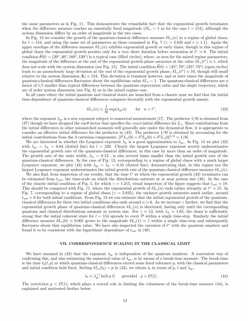
In Fig. 13 we consider the growth of the quantum-classical difference measure δLz(n) in a regime of global chaos,for l = 154, and using the same set of parameters as those examined in Fig. 7 (γ = 2.835 and r ≃ 1.1). Again theupper envelope of the difference measure δLz(n) exhibits exponential growth at early times, though in this regime ofglobal chaos the exponential growth persists only for a very short duration before saturation at t∗ ≃ 6. The initial

condition ~θ(0) = (20o, 40o, 160o, 130o) is a typical case (filled circles), where, as seen for the mixed regime parameters,the magnitude of the difference at the end of the exponential growth phase saturates at the value δLz(t

∗) ≃ 1, which

does not scale with the system dimension (see Fig. 15). The initial condition ~θ(0) = (45o, 70o, 135o, 70o) (open circles)leads to an anomolously large deviation at the end of the exponential growth phase, δLz(t

∗) ≃ 10, though still smallrelative to the system dimension |L| ≃ 154. This deviation is transient however, and at later times the magnitude ofquantum-classical differences fluctuates about the equilibrium value δLz ∼ 1. The quantum-classical differences are afactor of 1/l smaller than typical differences between the quantum expectation value and the single trajectory, whichare of order system dimension (see Fig. 6) as in the mixed regime case.

In all cases where the initial quantum and classical states are launched from a chaotic zone we find that the initialtime-dependence of quantum-classical differences compares favorably with the exponential growth ansatz,

δLz(n) ≃1

8lexp(λqcn) for n < t∗, (43)

where the exponent λqc is a new exponent subject to numerical measurement [17]. The prefactor 1/8l is obtained from(37) though we have dropped the cos θ factor that specifies the exact initial difference for Lz. Since contributions fromthe initial differences in other mismatched moments will generally mix under the dynamical flow, it is appropriate toconsider an effective initial difference for the prefactor in (43). The prefactor 1/8l is obtained by accounting for theinitial contributions from the 3 cartesian components, [δ2Lx(0) + δ2Ly(0) + δ2Lz(0]1/2 = 1/8l.

We are interested in whether the Lyapunov exponent λL is a good approximation to λqc. In Fig. 12 we plot (43)with λqc = λL = 0.04 (dotted line) for l = 220. Clearly the largest Lyapunov exponent severly underestimatesthe exponential growth rate of the quantum-classical differences, in this case by more than an order of magnitude.The growth rate of the state width, λw = 0.13 , is also several times smaller than the initial growth rate of thequantum-classical differences. In the case of Fig. 13, corresponding to a regime of global chaos with a much largerLyapunov exponent, we plot (43) with λqc = λL = 0.45 (dotted line), demonstrating that, in this regime too thelargest Lyapunov exponent underestimates the initial growth rate of the quantum-classical difference measure δLz(n).

We also find, from inspection of our results, that the time t∗ at which the exponential growth (43) terminates canbe estimated from tsat, the time-scale on which the distributions saturate at or near system size (40). In the caseof the chaotic initial condition of Fig. 5, for which γ = 1.215, visual inspection of the figure suggests that tsat ≃ 18.This should be compared with Fig. 11, where the exponential growth of δLz(n) ends rather abruptly at t∗ ≃ 15. InFig. 7, corresponding to a regime of global chaos (γ = 2.835), the variance growth saturates much earlier, aroundtsat ≃ 6 for both initial conditions. From Fig. 13 we can estimate that the initial exponential growth of the quantum-classical differences for these two initial conditions also ends around n ≃ 6. As we increase γ further, we find that theexponential growth phase of quantum-classical differences δLz(n) is shortened, lasting only until the correspondingquantum and classical distributions saturate at system size. For γ ≃ 12, with λL ≃ 1.65, the chaos is sufficientlystrong that the initial coherent state for l = 154 spreads to cover P within a single time-step. Similarly the initialdifference measure δLz(0) ≃ 0.001 grows to the magnitude δLz(1) ≃ 1 within a single time-step and subsequentlyfluctuates about that equilibrium value. We have also inspected the variation of t∗ with the quantum numbers andfound it to be consistent with the logarithmic dependence of tsat in (40).

VII. CORRESPONDENCE SCALING IN THE CLASSICAL LIMIT

We have assumed in (43) that the exponent λqc is independent of the quantum numbers. A convenient way ofconfirming this, and also estimating the numerical value of λqc, is by means of a break-time measure. The break-timeis the time tb(l, p) at which quantum-classical differences exceed some fixed tolerance p, with the classical parametersand initial condition held fixed. Setting δLz(tb) = p in (43), we obtain tb in terms of p, l and λqc,

tb ≃ λ−1qc ln(8 p l) provided p < O(1). (44)

The restriction p < O(1), which plays a crucial role in limiting the robustness of the break-time measure (44), isexplained and motivated further below.

12

The explicit form we have obtained for the argument of the logarithm in (44) is a direct result of our estimatethat the initial quantum-classical differences arising from the Cartesian components of the spin provide the dominantcontribution to the prefactor of the exponential growth ansatz (43). Differences in the mismatched higher ordermoments, as well as intrinsic differences between the quantum dynamics and classical dynamics, may also contributeto this effective prefactor. We have checked that the initial value δLz(0) ≃ 1/8l is an adequate estimate by comparingthe intercept of the quantum-classical data on a semilog plot with the prefactor of (43) for a variety of l values (seee.g. Fig. 12).

In Fig. 14 we examine the scaling of the break-time for l values ranging from 11 to 220 and with fixed tolerancep = 0.1. The break-time can assume only the integer values t = n and thus the data exhibits a step-wise behaviour. For

the mixed regime parameters, γ = 1.215 and r ≃ 1.1 (filled circles), with initial condition ~θ(0) = (20o, 40o, 160o, 130o),a non-linear least squares fit to (44) gives λqc = 0.43. This fit result is plotted in the figure as a solid line. Theclose agreement between the data and the fit provides good evidence that the quantum-classical exponent λqc isindependent of the quantum numbers. To check this result against the time-dependent δLz(n) data, we have plottedthe exponential curve (43) with λqc = 0.43 in Fig. 11 using a solid line and in Fig. 11 using a solid line for l = 22 anda dotted line for l = 220. The exponent obtained from fitting (44) serves as an excellent approximation to the initialexponential growth (43) of the quantum-classical differences in each case.

In Fig. 14 we also plot break-time results for the global chaos case γ = 2.835 and r ≃ 1.1 (open circles) with initial

condition ~θ(0) = (45o, 70o, 135o, 70o). In this regime the quantum-classical differences grow much more rapidly and,consequently, the break-time is very short and remains nearly constant over this range of computationally accessiblequantum numbers. Due to this limited variation, in this regime we can not confirm (44), although the data is consistentwith the predicted logarithmic dependence on l. Moreover, the break-time results provide an effective method forestimating λqc if we assume that (44) holds. The same fit procedure as detailed above yields the quantum-classicalexponent λqc = 1.1. This fit result is plotted in Fig. 14 as a solid line. More importantly, the exponential curve (43),plotted with fit result λqc = 1.1, can be seen to provide very good agreement with the initial growth rate of Fig. 13for either initial condition, as expected.

In the mixed regime (γ = 1.215), the quantum-classical exponent λqc = 0.43 is an order of magnitude greater thanthe largest Lyapunov exponent λL = 0.04 and about three times larger than the growth rate of the width λw = 0.13.In the regime of global chaos (γ = 2.835) the quantum-classical exponent λqc = 1.1 is a little more than twice as largeas the largest Lyapunov exponent λL = 0.45.

The condition p < O(1) is a very restrictive limitation on the domain of application of the log break-time (44) andit is worthwhile to explain the significance of this restriction. In the mixed regime case of Fig. 11, with l = 154, wehave plotted the tolerance values p = 0.1 (dotted line) and p = 15.4 (sparse dotted line). The tolerance p = 0.1 isexceeded at t = 11, while the quantum-classical differences are still growing exponentially, leading to a log break-timefor this tolerance value. For the tolerance p = 15.4 ≪ |L|, on the other hand, the break-time does not occur on ameasurable time-scale, whereas according to the logarithmic rule (44), with l = 154 and λqc = 0.43, we should expecta rather short break-time tb ≃ 23. Consequently the break-time (44), applied to delimiting the end of the Liouvilleregime, is not a robust measure of quantum-classical correspondence.

Our definition of the break-time (44) requires holding the tolerance p fixed in absolute terms (and not as fractionof system dimension as in [3]) when comparing systems with different quantum numbers. Had we chosen to comparesystems using a fixed relative tolerance, f , then the break-time would be of the form tb ≃ λ−1

qc ln(8 f l2) and subjectto the restriction f < O(1/l). Since f → 0 in the classical limit, this form emphasizes that the log break-time appliesonly to differences that are vanishing fraction of the system dimension in that limit.

Although we have provided numerical evidence (in Fig. 12) of one mixed regime case in which the largest quantum-classical differences occuring at the end of the exponential growth period remain essentially constant for varyingquantum numbers, δLz(t

∗) ∼ O(1), we find that this behaviour represents the typical case for all parameters andinitial conditions which produce chaos classically. To demonstrate this behaviour we consider the the scaling (withincreasing quantum numbers) of the maximum values attained by δLz(n) over the first 200 kicks, δLmax

z . Sincet∗ ≪ 200 over the range of l values examined, the quantity δLmax

z is a rigorous upper bound for δLz(t∗).

In Fig. 15 we compare δLmaxz for the two initial conditions of Fig. 13 and using the global chaos parameters

(γ = 2.835, r ≃ 1.1). The filled circles in Fig. 15 correspond to the initial condition ~θ(0) = (20o, 40o, 160o, 130o). Asin the mixed regime, the maximum deviations exhibit little or no scaling with increasing quantum number. This isthe typical behaviour that we have observed for a variety of different initial conditions and parameter values. Theseresults motivate the generic rule,

δL̃z(t∗) ≤ δL̃max

z ∼ O(1/l). (45)

Thus the magnitude of quantum-classical differences reached at the end of the exponential growth regime, expressedas a fraction of the system dimension, approaches zero in the classical limit.

13

However, for a few combinations of parameters and initial conditions we do observe a ‘transient’ discrepancy peakoccuring at t ≃ t∗ that exceeds O(1). This peak is quickly smoothed away by the subsequent relaxation of the quantumand classical distributions. This peak is apparent in Fig. 13 (open circles), corresponding to the most conspicuous casethat we have identified. This case is apparent as a small deviation in the normalized data of Fig. 6. The scaling of themagnitude of this peak with increasing l is plotted with open circles in Fig. 15. The magnitude of the peak initiallyincreases rapidly but appears to become asymptotically independent of l. The other case that we have observed occurs

for the classical parameters γ = 2.025, with r ≃ 1.1 and a = 5, and with initial condition ~θ(0) = (20o, 40o, 160o, 130o).We do not understand the mechanism leading to such transient peaks, although they are of considerable interest sincethey provide the most prominent examples of quantum-classical discrepancy that we have observed.

VIII. DISCUSSION

In this study of a non-integrable model of two interacting spins we have characterized the correspondence betweenquantum expectation values and classical ensemble averages for intially localised states. We have demonstrated that inchaotic states the quantum-classical differences initially grow exponentially with an exponent λqc that is consistentlylarger than the largest Lyapunov exponent. In a study of the moments of the Henon-Heiles system, Ballentine andMcRae [17,18] have also shown that quantum-classical differences in chaotic states grow at an exponential rate withan exponent larger than the largest Lyapunov exponent. This exponential behaviour appears to be a generic featureof the short-time dynamics of quantum-classical differences in chaotic states.

Since we have studied a spin system, we have been able to solve the quantum problem without truncation of theHilbert space, subject only to numerical roundoff, and thus we are able to observe the dynamics of the quantum-classical differences well beyond the Ehrenfest regime. We have shown that the exponential growth phase of thequantum-classical differences terminates well before these differences have reached system dimension. We find thatthe time-scale at which this occurs can be estimated from the time-scale at which the distribution widths approachthe system dimension, tsat ≃ (2λw)−1 ln(l) for initial minimum uncertainty states. Due to the close correspondencein the growth rates of the quantum and classical distributions, this time-scale can be estimated from the classicalphysics alone. This is useful because the computational complexity of the problem does not grow with the systemaction in the classical case. Moreover, we find that the exponent λw can be approximated by the largest Lyapunovexponent when the kinematic surface is predominantly chaotic.

We have demonstrated that the exponent λqc governing the initial growth rate of quantum-classical differencesis independent of the quantum numbers, and that the effective prefactor to this exponential growth decreases as1/l. These results imply that a log break-time rule (44) delimits the dynamical regime of Liouville correspondence.However, the exponential growth of quantum-classical differences persists only for short times and small differences,and thus this log break-time rule applies only in a similarly restricted domain. In particular, we have found that themagnitude of the differences occuring at the end of the initial exponential growth phase does not scale with the systemdimension. A typical magnitude for these differences, relative to the system dimension, is O(1/l). Therefore, log(l)break-time rules characterizing the end of the Liouville regime are not robust, since they apply to quantum-classicaldifferences only in a restricted domain, i.e. to relative differences that are smaller than O(1/l).

This restricted domain effect does not arise for the better known log break-time rules describing the end of theEhrenfest regime [1–3]. The Ehrenfest log break-time remains robust for arbitrarily large tolerances since the corre-sponding differences grow roughly exponentially until saturation at the system dimension [22,24]. Consequently, alog(l) break-time indeed implies a breakdown of Ehrenfest correspondence. However, the logarithmic break-time rulecharacterizing the end of the Liouville regime does not imply a breakdown of Liouville correspondence because itdoes not apply to the observation of quantum-classical discrepancies larger than O(1/l). The appearance of residualO(1/l) quantum-classical discrepancies in the description of a macroscopic body is, of course, consistent with quantummechanics having a proper classical limit.

We have found, however, that for certain exceptional combinations of parameters and initial conditions there arerelative quantum-classical differences occuring at the end of the exponential growth phase that can be larger thanO(1/l), though still much smaller than the system dimension. In absolute terms, these transient peaks seem togrow with the system dimension for small quantum numbers but become asymptotically independent of the systemdimension for larger quantum numbers. Therefore, even in these least favorable cases, the fractional differencesbetween quantum and classical dynamics approach zero in the limit l → ∞. This vanishing of fractional differencesis sufficient to ensure a classical limit for our model.

Finally, contrary to the results found in the present model, it has been suggested that a log break-time delimitingthe Liouville regime implies that certain isolated macroscopic bodies in chaotic motion should exhibit non-classicalbehaviour on observable time scales. However, since such non-classical behaviour is not observed in the chaotic motion

14

of macroscopic bodies, it is argued that the observed classical behaviour emerges from quantum mechanics only whenthe quantum description is expanded to include interactions with the many degrees-of-freedom of the ubiquitousenvironment [9,10]. (This effect, called decoherence, rapidly evolves a pure system state into a mixture that isessentially devoid of non-classical properties.) However, in our model classical behaviour emerges in the macroscopiclimit of a simple few degree-of-freedom quantum system that is described by a pure state and subject only to unitaryevolution. Quantum-classical correspondence at both early and late times arises in spite of the log break-time becausethis break-time rule applies only when the quantum-classical difference threshold is chosen smaller than O(h̄). In thissense we find that the decoherence effects of the environment are not necessary for correspondence in the macroscopiclimit. Of course the effect of decoherence may be experimentally significant in the quantum and mesoscopic domains,but it is not required as a matter of principle to ensure a classical limit.

IX. ACKNOWLEDGEMENTS

We wish to thank F. Haake and J. Weber for drawing our attention to the recursion algorithm for the rotationmatrix elements published in [23]. J. E. would like to thank K. Kallio for stimulating discussions.

X. APPENDIX

Ideally we would like to construct an initial classical density that reproduces all of the moments of the initialquantum coherent states. This is possible in a Euclidean phase space, in which case all Weyl-ordered moments ofthe coherent state can be matched exactly by the moments of a Gaussian classical distribution. However, below weprove that no classical density ρc(θ, φ) that describes an ensemble of spins of fixed length |J| can be constructedwith marginal distributions that match those of the SU(2) coherent states (21). Specifically, we consider the set ofdistributions on S2 with continuous independent variables θ ∈ [0, π] and φ ∈ [0, 2π), measure dµ = sin θdθdφ, andsubject to the usual normalization,

∫

S2

dµ ρc(θ, φ) = 1. (46)

For convenience we choose the coherent state to be polarized along the positive z-axis, ρ = |j, j〉〈j, j|. This state isaxially symmetric: rotations about the z-axis by an arbitrary angle φ leave the state operator invariant. Consequentlywe require axially symmetry of the corresponding classical distribution,

ρc(θ, φ) = ρc(θ). (47)

We use the expectation of the quadratic operator, 〈J2〉 = j(j + 1), to fix the length of the classical spins,

|J| =√

〈J2〉c =√

j(j + 1). (48)

Furthermore, the coherent state |j, j〉 is an eigenstate of Jz with moments along the z-axis given by 〈Jnz 〉 = jn for

integer n. Therefore we require that the classical distribution produces the moments,

〈Jnz 〉c = jn. (49)

These requirements are satisfied by the δ-function distribution,

ρv(θ) =δ(θ − θo)

2π sin θo, (50)

where cos θo = j/|J| defines θo. This distribution is the familiar vector model of the old quantum theory correspondingto the intersection of a cone with the surface of the sphere.

However, in order to derive an inconsistency between the quantum and classical moments we do not need to assumethat the classical distribution is given explicitly by (50); we only need to make use of the the azimuthal invariancecondition (47), the length condition (48), and the first two even moments of (49).

First we calculate some of the quantum coherent state moments along the x-axis (or any axis orthogonal to z),

15

〈Jmx 〉 = 0 for odd m

〈J2x〉 = j/2

〈J4x〉 = 3j2/4 − j/4.

In the classical case, these moments are of the form,

〈Jmx 〉c =

∫

dJz

∫

dφρc(θ)|J|m cosm(φ) sinm(θ). (51)

For m odd the integral over φ vanishes, as required for correspondence with the odd quantum moments. For m evenwe can evaluate (51) by expressing the r.h.s. as a linear combination of the z-axis moments (49) of equal and lowerorder. For m = 2 this requires substituting sin2(θ) = 1 − cos2(θ) into (51) and then integrating over φ to obtain

〈J2x〉c = π

∫

dJzρc(θ)|J|2 − π

∫

dJzρc(θ)|J|2 cos2(θ)

= |J|/2 − 〈J2z 〉/2.

Since 〈J2z 〉 is determined by (49) and the length is fixed from (48) we can deduce the classical value without knowing

ρ(θ),

〈J2x〉c = j/2. (52)

This agrees with the value of corresponding quantum moment. For m = 4, however, by a similar procedure we deduce

〈J4x〉c = 3j2/8, (53)

that differs from the quantum moment 〈J4x〉 by the factor,

δJ4x = |〈J4

x〉 − 〈J4x〉c| = |3j2/8 − j/4|, (54)

concluding our proof that no classical distribution on S2 can reproduce the quantum moments.

[1] L.E. Ballentine, Y. Yang, and J.P. Zibin, Phys. Rev. A 50, 2854 (1994).[2] G.P. Berman and G.M. Zaslavsky, Physica 91A, 450 (1978).[3] F. Haake, M. Kus and R. Scharf, Z. Phys. B 65, 361 (1987).[4] B.V. Chirikov, F.M. Israilev, and D.L. Shepelyansky, Physica D 33, 77 (1988).[5] W.H. Zurek and J.P. Paz, Phys. Rev. Lett. 72, 2508 (1994).[6] S. Habib, K. Shizume and W.H. Zurek, Phys. Rev. Lett. 80, 4361 (1998).[7] R. Roncaglia, L. Bonci, B.J. West, and P. Grigolini, Phys. Rev. E 51, 5524 (1995).[8] F. Haake, Quantum Signatures of Chaos (Springer-Verlag, New York, 1991).[9] W.H. Zurek and J.P. Paz, Phys. Rev. Letters 75, 351 (1995).

[10] W.H. Zurek, Physica Scripta T76, 186 (1998).[11] M. Feingold and A. Peres, Physica 9D 433 (1983).[12] L. E. Ballentine, Phys. Rev. A 44, 4126 (1991).[13] L. E. Ballentine, Phys. Rev. A 44, 4133 (1991).[14] L. E. Ballentine, Phys. Rev. A 47, 2592 (1993).[15] D. T. Robb and L. E. Reichl, Phys. Rev. E 57, 2458 (1998).[16] G.J. Milburn, quant-ph/9908037 (1999).[17] L.E. Ballentine and S.M. McRae, Phys. Rev. A 58, 1799 (1998).[18] L.E. Ballentine, Phys. Rev. A 63, 024101 (2001).[19] J.J. Sakurai, Modern Quantum Mechanics (Benjamin-Cummings, Menlo Park Calif., 1985).[20] A.J. Lichtenberg and M.A. Lieberman, Regular and Chaotic Motion (Springer-Verlag, New York, 1992).[21] A. Perelomov, Generalized Coherent States and Their Applications, (Springer-Verlag, New York , 1986).[22] R.F. Fox and T.C. Elston, Phys. Rev. E 50, 2553 (1994).[23] A. Braun, P. Gerwinski, F. Haake, H. Schomerus, Z. Phys. B 100, 115 (1996).

16

[24] R.F. Fox and T.C. Elston, Phys. Rev. E 49, 3683 (1994).[25] B.S. Helmkamp and D.A. Browne, Phys. Rev. E 49, 1831 (1994).[26] J.R. Dorfman, An Introduction to Chaos in NonEquilibrium Statistical Mechanics (Cambridge University Press, Cambridge,

1999).[27] J. Emerson and L.E. Ballentine, submitted to Phys. Rev. E, quant-ph/0103050 (2001).

17

1

10

100

0 0.5 1 1.5 2 2.5 3 3.5 4

r

γ

Regular Dynamics

c c

c c

c c

c c

cc

c c

c c

c c

c c

c c

c c

c c

c

c

c c

c c

c

c c

c

c

c c

c c c c c c c c

c c c c c c c c

c c c c c c c c

c c c

c c

c c

c c c c c c c c

c c c c c c c c

c

c

c c c c c c c c

c

c

c c c c c c

c c c c c c

c c c c c c

c c c

cc c c c c c c c c c

c c c c c c c

c c c c c c

c c c

c

c c

c c c c

c

Chaotic Dynamics

×

××××

×××

××××××××××××

×

××××××

×××××

××××××××

××××××××

××××××××××××××××

×××××××××××

××××××××××××××××

××××××

××××××××××××××××

×××××××××××××××

××××××××

××××××××

××××××××××××××××

××××××××

× ×××××××××××××××××××××××××××××××

××××××××××

××××××××××

××××××××××××××××××××

××××××××××××××××××××

××××××××××××××××××××

××××××××××

××××××××××××××××××××

××××××××××××××××××××

××××××××××

××××××××××

××××××××××××××××××××

××××××××××

××××××××××××××××××××××××××××××

××××××××××

×

××××××××××××××××××××

××××××××××××××××××××

××××××××××××××××××××

××××××××××

×××××××××××

××××××××××××××××××××

×

××××××××××

××

××××××××××

××××××××××××××××××××××××××××××

××××××××××××××××××××××××××××××

××××××××××××××××××××

××××××××××××××××××××

××××××××××

××××××××××

××××××××××××××××××××××××××××××××××××××××

×

s s

FIG. 1. Behaviour of the classical mapping for different values of r = |L|/|S| and γ = c|S| with a = 5. Circles correspond toparameter values for which at least 99% of the surface area P produces regular dynamics and crosses correspond to parametervalues for which the dynamics are at least 99% chaotic. Superpositions of circles and crosses correspond to parameter valueswhich produce a mixed phase space. We investigate quantum-classical correspondence for the parameter values γ = 1.215(mixed regime) and γ = 2.835 (global chaos), with r = 1.1, which are indicated by filled circles.

L̃z

1

0

-1

L̃y

1

0

-1L̃x1

0

-1

S̃z

1

0

-1

S̃y

1

0

-1S̃x1

0

-1

FIG. 2. Stroboscopic trajectories on the unit sphere launched from a regular zone of the mixed regime with γ = 1.215,r = 1.1, a = 5 and ~θ(0) = (5o, 5o, 5o, 5o).

18

L̃z

1

0

-1

L̃y

1

0

-1L̃x1

0

-1

S̃z

1

0

-1

S̃y

1

0

-1S̃x1

0

-1

FIG. 3. Same parameters as Fig. 2 but the trajectory is launched from a chaotic zone of the mixed regime with initialcondition ~θ(0) = (20o, 40o, 160o, 130o).

L̃z

1

0

-1

L̃y

1

0

-1L̃x1

0

-1

S̃z

1

0

-1

S̃y

1

0

-1S̃x1

0

-1

FIG. 4. A chaotic trajectory for mixed regime parameters γ = 0.06, r = 100, and a = 5 with ~θ(0) = (27o, 27o, 27o, 27o). Themotion of the larger spin appears to remain confined to a narrow band on the surface of the sphere.

19

0.01

0.1

1

0 10 20 30 40 50

∆L̃2

Kick Number

quantum (a)

3

3

3

3

3

33

3

3

3

3

3

33

3

3

33

3

33

333

3

3

33

333333

33333333333333333

3

quantum (b)

+

++++

+++

+

+++

++

++++

+++

++++

+++++++++

+++++++

++++

+++++

+

+classical (a)

2

2

2

2

2

22

2

2

2

2

2

22

2

2

22

2

22

222

2

2

22

222222

22222222222222222

2

classical (b)

×

××××

×××

×

×××

××

××××

×××

××××

×××××××××

×××××××

××××××

××××

×

FIG. 5. Growth of normalized quantum and classical variances in a chaotic zone (a) and a regular zone (b) of the mixedphase space regime γ = 1.215 and r ≃ 1.1 with l = 154. Quantum and and classical results are nearly indistinguishable onthis scale. In the chaotic case, the approximately exponential growth of both variances is governed by a much larger rate,λvar = 0.13 (solid line), than that predicted from the largest Lyapunov exponent, λL = 0.04 (dotted line).

-1

-0.8

-0.6

-0.4

-0.2

0

0.2

0.4

0.6

0.8

1

0 5 10 15 20 25 30 35

〈L̃z〉

Kick Number

Classical Averagec

cc

c

c

c

c

c

c

c

c c

c

c

c

c

c

c cc c c c c c c c c c c c c c c c c

c

Quantum Expectations

ss

s

s

s

s

s

s

s

s

s

s

s

s

s

s

s ss s

s s s s s s s s s s s s s s s

s

Single Trajectory

+

++

+

+

++

++

+

+

+

+

+++

+

+

+

+

+

+

+

+

+

++

+

++

+

++

+

+

+

+

FIG. 6. Comparison of quantum expectation value and corresponding classical average 〈Lz〉c in the regime of global chaos

γ = 2.835 and r ≃ 1.1 with l = 154 and initial condition ~θo = (45o, 70o, 135o, 70o). The points of the stroboscopic map areconnected with lines to guide the eye. The quantum expectation value and the Liouville average exhibit esentially the samerate of relaxation to microcanonical equilibrium, a behaviour which is qualitatively distinct from that of the single trajectory.

20

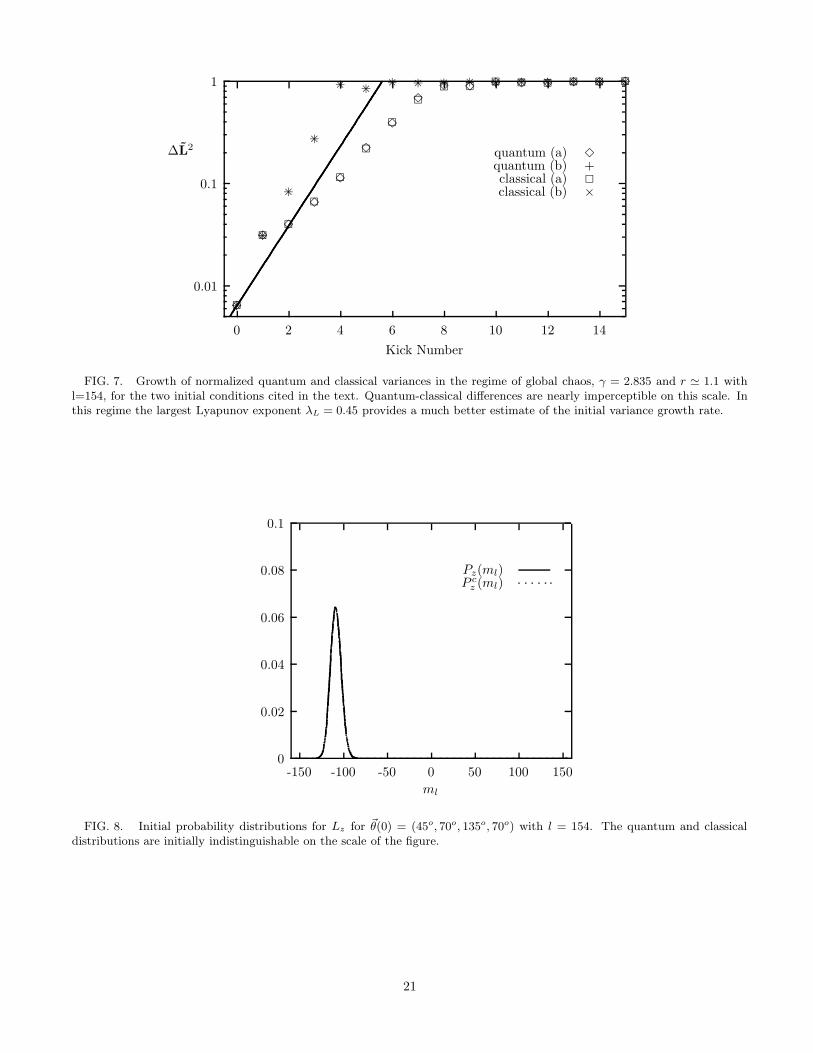
0.01

0.1

1

0 2 4 6 8 10 12 14

∆L̃2

Kick Number

quantum (a)

3

33

3

3

3

3

3

3 3 3 3 3 3 3 3

3

quantum (b)

+

+

+

+

+ + + + + + + + + + + +

+classical (a)

2

22

2

2

2

2

2

2 2 2 2 2 2 2 2

2

classical (b)

×

×

×

×

× × × × × × × × × × × ×

×

FIG. 7. Growth of normalized quantum and classical variances in the regime of global chaos, γ = 2.835 and r ≃ 1.1 withl=154, for the two initial conditions cited in the text. Quantum-classical differences are nearly imperceptible on this scale. Inthis regime the largest Lyapunov exponent λL = 0.45 provides a much better estimate of the initial variance growth rate.

0

0.02

0.04

0.06

0.08

0.1

-150 -100 -50 0 50 100 150

ml

Pz(ml)P c

z (ml)

FIG. 8. Initial probability distributions for Lz for ~θ(0) = (45o, 70o, 135o, 70o) with l = 154. The quantum and classicaldistributions are initially indistinguishable on the scale of the figure.

21

0

0.005

0.01

0.015

0.02

-150 -100 -50 0 50 100 150

ml

Pz(ml)P c

z (ml)

FIG. 9. Same as Fig. 8 but the states have evolved to n = 6 in the regime of global chaos γ = 2.835 and r ≃ 1.1. Boththe quantum and classical distribution have spread to system dimension and exhibit their largest differences on this saturationtime-scale.

0

0.005

0.01

0.015

0.02

-150 -100 -50 0 50 100 150

ml

Pz(ml)P c

z (ml)

FIG. 10. Same as Fig. 9, but for n = 15. Both quantum and classical distributions have relaxed close to the microcanonicalequilibrium.

22

0.001

0.01

0.1

1

10

100

0 50 100 150 200

δLz

Kick Number

r

r

r

r

r

r

r

r

r

rrr

r

r

rrr

r

r

r

r

rr

rr

rr

r

r

r

r

r

r

r

rr

rrr

r

r

r

rr

r

r

r

rr

r

r

rr

rr

r

rrr

rrr

r

rrrr

r

r

r

rrrrr

r

rrrrr

rr

rrrrrr

rr

rrrr

r

r

r

rrrrr

r

r

r

rrrr

r

r

r

rrrrr

r

r

rrrr

rr

r

rrrr

r

r

rrrr

r

r

rrrrr

rr

rrrr

rr

rrrrr

rr

rrrr

r

r

rrrrr

r

r

rrrr

rr

r

rrr

rr

r

rrrrr

rrrrrrr

r

r

r

bb

b

b

bbbbb

b

b

bb

b

bb

b

b

bb

b

bb

b

bb

bb

b

bb

bb

b

b

b

b

bbbbb

b

b

bb

b

b

b

b

b

bbbbb

b

bbbbb

b

b

b

b

b

b

b

b

b

bbbbb

b

b

b

b

bb

bb

b

b

b

b

b

b

bbbbbb

b

b

b

b

b

b

b

bbbb

b

b

bbbbb

b

b

b

b

b

b

b

b

b

bbbbb

b

b

b

b

b

b

bb

bb

b

b

b

b

bbbbbb

b

b

b

b

bb

b

b

b

bbbb

b

bb

b

bb

bb

b

b

b

bb

b

bb

b

bb

bb

b

b

b

bb

b

bb

b

bbbb

b

b

b

b

++

++

+

+

++

+++++

++

+++++

+

+++

+

++++++++++++++++++

+

++++++++

+

+++++++++++++

+++++++++++

+++++++

+

+++++

+

+++++++++++++++++

+++++++

++++++

+

+++++

+

+++++

+

+++++

+

++++++

++++++++++++

++++++

++++++

+

+++++++++++++++++++

++

++++

+

+

++

FIG. 11. Time-dependence of quantum-classical differences in a regular zone (open circles) and a chaotic zone (filled circles)of mixed regime (γ = 1.215 and r ≃ 1.1) with l = 154. For the chaotic state δLz = |〈Lz〉 − 〈Lz〉c| is compared with theEhrenfest difference, |〈Lz〉−Lz|, between the quantum expectation value and a single trajectory (plus signs), which grows untilsaturation at system dimension. The solid line corresponds to (43) using λqc = 0.43. The horizontal lines indicate two differentvalues of the difference tolerance p which may be used to determine the break-time; for p = 0.1 (dotted line) tb occurs on alogarithmic time-scale, but for p = 15.4 (sparse dotted line) tb is not defined over numerically accessible time-scales.

0.001

0.01

0.1

1

10

0 5 10 15 20 25 30 35

δLz

Kick Number

s s

s

s

s

s

s

s

s

s

s

s

s

ss

s

s

s

ss

s

s

s

s ss s

ss

s s

s

s

s

s

s

cc

c

c

c

c

c

c

cc

c

c

c

c

c

cc

cc

c

c

c

c

c

c

c

cc

cc

c c

c

c

c

c

FIG. 12. Growth of the quantum-classical difference δLz in the chaotic zone of a mixed regime, γ = 1.215 and r ≃ 1.1, withl = 22 (filled circles) and l = 220 (open circles). For l = 220 the exponential growth rate (43) is plotted using the classicalLyapunov exponent, λL = 0.04 (sparse dotted line), and for both l values (43) is plotted using the exponent λqc = 0.43 (solidline for l = 22, dotted line for l = 220), which is obtained from a fit of (44) to the corresponding break-time data in Fig. 14.

23

0.001

0.01

0.1

1

10

0 5 10 15 20 25 30 35

δLz

Kick Number

s

s

ss

s

s

s

s

s

s

s

s

s

s

s

s

s

s

s

s

s

s

s

ss

s

ss

s

s

s

ss

s

ss

cc

c

c

c

c

c

c

c

c

c

c

c

cc

c c

c

c

cc c

c

c c

c

c

c

c

c

cc

c

c

c

c

FIG. 13. Growth of quantum-classical differences in the regime of global chaos γ = 2.835 and r ≃ 1.1 with l = 154 forthe two initial conditions cited in text. The exponential growth rate (43) is plotted using the classical Lyapunov exponent,λL = 0.45 (dotted line), and the exponent λqc = 1.1 (solid line), which is obtained from a fit of (44) to the correspondingbreak-time data in Fig. 14.

2

4

6

8

10

12

0 50 100 150 200 250

tb

l

c

c c c c c c c c c c

s

s

s s s s

s s s s s s s

s s s s

s s s

FIG. 14. Scaling of the break-time using tolerance p = 0.1 as a function of increasing quantum number for the mixedregime parameters γ = 1.215 and r ≃ 1.1 with ~θ(0) = (20o, 40o, 160o, 130o) (filled circles) and for the global chaos parameters

γ = 2.835 and r ≃ 1.1 with ~θ(0) = (45o, 70o, 135o, 70o) (open circles). We also plot the results of fits to the log rule (44), whichproduced exponents λqc = 0.43 for γ = 1.215 and λqc = 1.1 for γ = 2.835.

24

0.1

1

10

100

0 50 100 150 200 250

δLmaxz

l

s s ss

s

s s s s

s s s s

s ss s

ss

ss

s

s s s

c

c

cc

c

c c c

cc

cc

c

cc

cc c c

c c c c c c

FIG. 15. Maximum quantum-classical difference occuring over the first 200 kicks in the regime of global chaos (γ = 2.835,r ≃ 1.1) plotted against increasing quantum number. These maximum values provide an upper bound on δLz(t

∗) for each l.

The data corresponding to the initial condition ~θ(0) = (20o, 40o, 160o, 130o) (filled circles) represent a typical case in which themaximum quantum-classical differences do not vary significantly with l. The large deviations observed for the initial condition~θ(0) = (45o, 70o, 135o, 70o) (open circles) are an exceptional case, with maximum differences growing rapidly for small quantumnumbers but tending asymptotically toward independence of l. These curves provide an upper bound on the tolerance valuesp for which the break-time measure scales logarithmicly with l.

25