
Sensing single spins with colour centres in diamond - OPARU
185
Sensing single spins with colour centres in diamond DISSERTATION zur Erlangung des Doktorgrades Dr. rer. nat. der Fakultät für Naturwissenschaften der Universität Ulm vorgelegt von Christoph Müller aus Leutkirch 2016
-
Upload
khangminh22 -
Category
Documents
-
view
2 -
download
0
Transcript of Sensing single spins with colour centres in diamond - OPARU

Sensing single spins with colourcentres in diamond
DISSERTATIONzur Erlangung des Doktorgrades Dr. rer. nat.
der Fakultät für Naturwissenschaften der Universität Ulm
vorgelegt vonChristoph Müller
aus Leutkirch
2016

Amtierender Dekan: Prof. Dr. Peter Dürre
Erstgutachter: Prof. Dr. Fedor Jelezko
Zweitgutachter: PD Dr. Boris Naydenov
Tag der Promotion: 07. 07. 2016
version of 12th July 2016
© 2016 - Christoph Müller

Abstract
This thesis reports on recent progress in magnetometry based on the negativelycharged nitrogen-vacancy colour centre in diamond. The main focus is thereby thedetection of single external nuclear spins.The nitrogen-vacancy (NV) centre is a point defect in diamond, consisting of a
substitutional nitrogen atom and an adjacent vacancy in the diamond lattice. Itselectronic spin state can be initialised and read out by means of green laser lightand coherently manipulated by microwave irradiation. Additionally, it possesseslong coherence times even at room temperature.During the last decade the NV centre attracted attention as a high-sensitivity
nanoscale NMR sensor. In this work, improvements in the sensitivity are shown,leading to detection volumes down to (2 nm)3, where the detected signal was evokedby around 20 statistically polarised hydrogen spins. In the so-called strong couplingregime, where the interaction between NV sensor and sample spins is the most dom-inant one, we located individual 29Si nuclear spins with sub-nanometre resolutionand obtained single nuclear spin sensitivity within seconds.In addition, the surface noise experienced by shallow NV centres is probed and
efficient decoupling from the noise is demonstrated, which allowed to obtain longercoherence times and therefore a better spectral resolution of the NV sensor.In a further experiment, the successful creation of a strongly coupled pair of NV
centres is shown. This is an important step towards arrays of strongly coupled NVcentres, which in the end may act as a quantum computer.
iii


Contents
List of Figures ix
List of Tables xiii
1 Introduction 1
2 The Nitrogen-Vacancy Centre in Diamond 72.1 Diamond . . . . . . . . . . . . . . . . . . . . . . . . . . . . . . . . . . 7
2.1.1 Physical properties . . . . . . . . . . . . . . . . . . . . . . . . 82.1.2 Synthetic diamonds . . . . . . . . . . . . . . . . . . . . . . . . 102.1.3 Colour centres in diamond . . . . . . . . . . . . . . . . . . . . 11
2.2 The nitrogen-vacancy centre . . . . . . . . . . . . . . . . . . . . . . . 122.2.1 Electronic structure . . . . . . . . . . . . . . . . . . . . . . . . 132.2.2 Optical properties . . . . . . . . . . . . . . . . . . . . . . . . . 142.2.3 NV centre Hamiltonian . . . . . . . . . . . . . . . . . . . . . . 172.2.4 Optically detected magnetic resonance . . . . . . . . . . . . . 21
2.3 NV centre spin dynamics . . . . . . . . . . . . . . . . . . . . . . . . . 232.3.1 Bloch sphere representation . . . . . . . . . . . . . . . . . . . 232.3.2 Rabi oscillations . . . . . . . . . . . . . . . . . . . . . . . . . . 242.3.3 T1 relaxation time . . . . . . . . . . . . . . . . . . . . . . . . . 252.3.4 T ∗2 dephasing time – free induction decay . . . . . . . . . . . . 272.3.5 T2 coherence time – the Hahn-echo sequence . . . . . . . . . . 282.3.6 Dynamical decoupling . . . . . . . . . . . . . . . . . . . . . . 29
2.4 Shallow NV centres . . . . . . . . . . . . . . . . . . . . . . . . . . . . 312.4.1 Creation of shallow NV centres . . . . . . . . . . . . . . . . . 322.4.2 Spin properties of very shallow NV centres . . . . . . . . . . . 342.4.3 Charge stability and surface treatment . . . . . . . . . . . . . 34
v

Contents
3 Nuclear Magnetic Resonance and Magnetometry 373.1 Principles of nuclear magnetic resonance . . . . . . . . . . . . . . . . 37
3.1.1 Basic theory . . . . . . . . . . . . . . . . . . . . . . . . . . . . 383.1.2 Classical NMR . . . . . . . . . . . . . . . . . . . . . . . . . . 403.1.3 Chemical shift . . . . . . . . . . . . . . . . . . . . . . . . . . . 41
3.2 Nanoscale magnetometry . . . . . . . . . . . . . . . . . . . . . . . . . 423.3 Magnetometry with nitrogen-vacancy centres . . . . . . . . . . . . . . 43
3.3.1 DC field sensing with NV centres . . . . . . . . . . . . . . . . 433.3.2 AC field sensing with NV centres . . . . . . . . . . . . . . . . 44
4 Strongly Coupled Nitrogen-Vacancy Centres 494.1 Sample preparation and characterisation . . . . . . . . . . . . . . . . 50
4.1.1 NV pair creation . . . . . . . . . . . . . . . . . . . . . . . . . 514.1.2 Creation efficiency . . . . . . . . . . . . . . . . . . . . . . . . 52
4.2 Strongly coupled NV pair . . . . . . . . . . . . . . . . . . . . . . . . 544.2.1 NV pair Hamiltonian . . . . . . . . . . . . . . . . . . . . . . . 564.2.2 Double electron-electron resonance measurements . . . . . . . 564.2.3 Alternating Ramsey measurements . . . . . . . . . . . . . . . 58
5 Sensing of External Spins 615.1 Noise spectroscopy . . . . . . . . . . . . . . . . . . . . . . . . . . . . 62
5.1.1 Statistical polarisation . . . . . . . . . . . . . . . . . . . . . . 625.1.2 XY8 sensing . . . . . . . . . . . . . . . . . . . . . . . . . . . . 645.1.3 The filter function . . . . . . . . . . . . . . . . . . . . . . . . 66
5.2 Spectral decomposition . . . . . . . . . . . . . . . . . . . . . . . . . . 675.3 Detection of external hydrogen spins . . . . . . . . . . . . . . . . . . 695.4 Identification of shallow NV centres . . . . . . . . . . . . . . . . . . . 72
5.4.1 Depth calculation . . . . . . . . . . . . . . . . . . . . . . . . . 74
6 Single Spin Sensing 796.1 Sample preparation and characterisation . . . . . . . . . . . . . . . . 80
6.1.1 Detection of external silicon spins . . . . . . . . . . . . . . . . 806.2 Strong coupling regime . . . . . . . . . . . . . . . . . . . . . . . . . . 826.3 Resolving the position of individual nuclei . . . . . . . . . . . . . . . 85
6.3.1 Basis pursuit de-noising . . . . . . . . . . . . . . . . . . . . . 86
vi

Contents
6.4 Single nuclear spin sensitivity . . . . . . . . . . . . . . . . . . . . . . 91
7 Spectroscopy of Surface-Induced Noise 937.1 Sample characterisation . . . . . . . . . . . . . . . . . . . . . . . . . 947.2 T2 scaling under CPMG dynamical decoupling . . . . . . . . . . . . . 967.3 Spectral decomposition . . . . . . . . . . . . . . . . . . . . . . . . . . 997.4 Depth dependency . . . . . . . . . . . . . . . . . . . . . . . . . . . . 1037.5 Conclusion . . . . . . . . . . . . . . . . . . . . . . . . . . . . . . . . . 104
8 Conclusion and Outlook 1078.1 Conclusion . . . . . . . . . . . . . . . . . . . . . . . . . . . . . . . . . 1078.2 Outlook . . . . . . . . . . . . . . . . . . . . . . . . . . . . . . . . . . 108
A Experimental Setup 113A.1 Confocal microscope . . . . . . . . . . . . . . . . . . . . . . . . . . . 113A.2 Microwave setup . . . . . . . . . . . . . . . . . . . . . . . . . . . . . 116A.3 Data acquisition and normalisation . . . . . . . . . . . . . . . . . . . 117
A.3.1 Data acquisition . . . . . . . . . . . . . . . . . . . . . . . . . . 117A.3.2 Data normalisation . . . . . . . . . . . . . . . . . . . . . . . . 118
A.4 Magnetic field alignment . . . . . . . . . . . . . . . . . . . . . . . . . 119A.4.1 Fluorescence alignment . . . . . . . . . . . . . . . . . . . . . . 121
B Abbreviations and Symbols 123B.1 Abbreviations . . . . . . . . . . . . . . . . . . . . . . . . . . . . . . . 123B.2 Symbols . . . . . . . . . . . . . . . . . . . . . . . . . . . . . . . . . . 124
Bibliography 127
Acknowledgements 159
List of Publications 163
Curriculum Vitae 169
Erklärung 171
vii


List of Figures
2.1 Diamond gemstone . . . . . . . . . . . . . . . . . . . . . . . . . . . . 82.2 Diamond lattice and carbon phase diagram . . . . . . . . . . . . . . . 92.3 The four possible NV centre orientations . . . . . . . . . . . . . . . . 132.4 NV centre energy level scheme . . . . . . . . . . . . . . . . . . . . . . 152.5 Spin state dependent fluorescence . . . . . . . . . . . . . . . . . . . . 162.6 Antibunching measurement . . . . . . . . . . . . . . . . . . . . . . . 172.7 NV energy level scheme with hypefine splitting . . . . . . . . . . . . . 192.8 Optically detected magnetic resonance . . . . . . . . . . . . . . . . . 222.9 Bloch sphere representation . . . . . . . . . . . . . . . . . . . . . . . 242.10 Rabi oscillations . . . . . . . . . . . . . . . . . . . . . . . . . . . . . . 252.11 Relaxation time . . . . . . . . . . . . . . . . . . . . . . . . . . . . . . 262.12 The Ramsey sequence . . . . . . . . . . . . . . . . . . . . . . . . . . 272.13 The Hahn echo sequence . . . . . . . . . . . . . . . . . . . . . . . . . 292.14 The CPMG sequence . . . . . . . . . . . . . . . . . . . . . . . . . . . 302.15 The XY8 sequence . . . . . . . . . . . . . . . . . . . . . . . . . . . . 312.16 SRIM simulations . . . . . . . . . . . . . . . . . . . . . . . . . . . . . 33
3.1 Nuclear spin in an external magnetic field . . . . . . . . . . . . . . . 393.2 Scheme of a classical NMR setup . . . . . . . . . . . . . . . . . . . . 41
4.1 Strongly coupled pair of NV centres . . . . . . . . . . . . . . . . . . . 494.2 SRIM simulations for nitrogen and carbon co-implantation . . . . . . 514.3 NV pair creation and coupling strength . . . . . . . . . . . . . . . . . 524.4 NV pair confocal images . . . . . . . . . . . . . . . . . . . . . . . . . 534.5 ODMR spectrum of the coupled NV pair . . . . . . . . . . . . . . . . 554.6 Hahn echo on the pair NV centres . . . . . . . . . . . . . . . . . . . . 564.7 DEER measurements on the coupled NV pair . . . . . . . . . . . . . 574.8 Alternating Ramsey on NVJ . . . . . . . . . . . . . . . . . . . . . . . 59
ix

List of Figures
4.9 Alternating Ramsey on NVK . . . . . . . . . . . . . . . . . . . . . . . 60
5.1 Sensing example . . . . . . . . . . . . . . . . . . . . . . . . . . . . . . 615.2 Magnetic field from statistically polarised spins . . . . . . . . . . . . 645.3 Noise spectroscopy with the XY8 sequence . . . . . . . . . . . . . . . 655.4 Typical signal for XY8 sensing . . . . . . . . . . . . . . . . . . . . . . 665.5 Filter function of the XY8 sequence . . . . . . . . . . . . . . . . . . . 675.6 Signal reconstruction by deconvolution . . . . . . . . . . . . . . . . . 685.7 Confocal image of sample 69 . . . . . . . . . . . . . . . . . . . . . . . 695.8 Magnetic field dependency of the hydrogen signal . . . . . . . . . . . 705.9 Linewidth of the hydrogen NMR signal . . . . . . . . . . . . . . . . . 715.10 Power spectral density reconstruction of the hydrogen signal . . . . . 735.11 Power spectral density reconstruction of the hydrogen signal of NV6 . 755.12 Depth and number of detected hydrogen spins of NV6 . . . . . . . . 76
6.1 Sensing silicon nuclear spins . . . . . . . . . . . . . . . . . . . . . . . 796.2 Magnetic field dependency of the silicon signal . . . . . . . . . . . . . 816.3 The three different sensing regimes . . . . . . . . . . . . . . . . . . . 836.4 Simulations of the expected echo decay . . . . . . . . . . . . . . . . . 846.5 Inhomogeneous broadening of the silicon signal . . . . . . . . . . . . . 856.6 Determination of the background noise spectrum . . . . . . . . . . . 876.7 Signal contribution of individual spins . . . . . . . . . . . . . . . . . 886.8 Contributions of the four strongest contributing spins . . . . . . . . . 896.9 Positions of the four strongest contributing spins . . . . . . . . . . . . 906.10 Single spin sensitivity . . . . . . . . . . . . . . . . . . . . . . . . . . . 91
7.1 Surface spins affecting the NV centres . . . . . . . . . . . . . . . . . . 937.2 Confocal images of sample 69 and sample 70 . . . . . . . . . . . . . . 957.3 Depth dependency of the coherence time . . . . . . . . . . . . . . . . 967.4 Scaling of the coherence time with the number of decoupling pulses . 987.5 Noise spectra for different NV centres . . . . . . . . . . . . . . . . . . 1007.6 Comparison of different fit-functions . . . . . . . . . . . . . . . . . . . 1007.7 Comparison of noise spectra for different parameters . . . . . . . . . . 1027.8 Bath coupling strengths . . . . . . . . . . . . . . . . . . . . . . . . . 104
x

List of Figures
A.1 The confocal microscope . . . . . . . . . . . . . . . . . . . . . . . . . 114A.2 Confocal images of single NV centres . . . . . . . . . . . . . . . . . . 115A.3 Pulsed Setup . . . . . . . . . . . . . . . . . . . . . . . . . . . . . . . 117A.4 Data acquisition example . . . . . . . . . . . . . . . . . . . . . . . . . 118A.5 Normalisation process . . . . . . . . . . . . . . . . . . . . . . . . . . 119A.6 Dependency of ν± on magnetic field B and misalignment θ . . . . . . 120A.7 Energy scheme of the NV electron spin ground and excited state . . . 121
xi


List of Tables
2.1 Nitrogen hyperfine parameters . . . . . . . . . . . . . . . . . . . . . . 212.2 Typical NV centre coherence times . . . . . . . . . . . . . . . . . . . 28
3.1 Gyromagnetic ratios and natural abundance of different isotopes . . . 40
4.1 NV centre creation efficiency . . . . . . . . . . . . . . . . . . . . . . . 54
5.1 Estimated NV centre depths . . . . . . . . . . . . . . . . . . . . . . . 77
7.1 Properties of the measured NV centres . . . . . . . . . . . . . . . . . 977.2 Saturated coherence times and relaxation times . . . . . . . . . . . . 997.3 Coupling strength obtained from normal fitting . . . . . . . . . . . . 1037.4 Coupling strength obtained from global fitting . . . . . . . . . . . . . 105
xiii


1 Introduction
Nuclear magnetic resonance (NMR) [1, 2] is one of the most powerful tools formeasuring the structure and chemical composition of molecules. Therefore it iswidely used as an analytical tool in the natural sciences and in medicine, whereit builds the basis for magnetic resonance imaging [3]. In theory, NMR enablessingle spin sensitivity. However, in classical NMR devices, the resolution is limitedby the sensitivity of the induction coil that measures the NMR signal. The lowsensitivity together with the low Boltzmann polarisation, on which the detection isbased restricts NMR to averaged signals from large numbers of molecules (typically1016 – 1018 spins are needed [4]) and leads to spatial resolutions that are limited toaround 10 µm in magnetic resonance imaging (MRI) [5] and are usually in the lowermillimetre range for clinical MRI machines. That means, that for achieving a betterresolution, one has to develop a different detection method.Almost ten years ago, a new detection method based on the negatively charged
nitrogen-vacancy (NV) centre was proposed as a system that is capable to detectvery small NMR signals [6, 7, 8]. The NV centre is a point defect in diamondconsisting of a substitutional nitrogen atom together with an adjacent vacancy [9].The first measurement of individual NV centres was shown by Gruber et al. [10] in
1997 and in 2000, Kurtsiefer et al. [11] performed the first experiments that proofedthat NV centres are single photon sources.Several remarkable properties are making the NV centre one of the most promising
system for sensing applications. In addition to its high sensitivity for small signals,its atomic size allows very precise positioning of the sensor. Further more, in 2004 theNV centre gained more attention, when Jelezko et al. showed coherent manipulationand optical readout of its spin state [12, 13], which paved the way for single electronspin resonance (ESR) experiments. These features come together with remarkablyhigh photostability and long spin coherence times up to the millisecond range atroom temperature [14].
1

1 Introduction
Up to now a variety of experimental realisations with NV centres as sensorshas been demonstrated, like the detection of magnetic [8, 15, 16, 17] and electricfields [18] or the measurements of pressure [19] and temperature [20, 21, 22]. Evenin biology [23, 24, 25], where possible applications are the tracking of orientationand location of fluorescent nanodiamonds with nanoscale precision [26], magneticimaging of cells with high resolution [27, 28] or the noninvasive detection of neuronactivities [29, 30] the NV centre attracts more and more attention. Further applic-ations can be found in quantum computation [31, 32], where for example Grover’salgorithm for fast searching was successfully implemented with NV centres [33]. Theheart of such an NV centre based quantum processor would be an array of coupledNV centres.
In this thesis we report on the successful creation and measurement of a stronglycoupled pair of NV centres with exceptional long coherence times. Such a stronglycoupled pair can act as the simplest form of an array of quantum bits and coupledNV centres may also be used for entanglement assisted sensing [34, 35].
Beside the measurements on the strongly coupled pair, this work mainly dealswith the NV centre being used as a nanoscale magnetometer, with the ultimate goalof the detection of single external nuclear spins. An atomic-sized magnetometeras the NV centre, together with the ability to detect individual nuclear spins caneventually enable single-molecule NMR spectroscopy [36, 37] with the ability toobtain information about the actual chemical composition and structure of a singlemolecule [38].
Different publications already demonstrated the ability to detect the position ofindividual 13C nuclear spins inside diamond [39, 40, 41], single and small ensemblesof electronic spins outside the diamond [42, 43, 44] as well as small ensembles ofexternal nuclear spins [45, 46], where 104 nuclear spins in a volume of (5 nm)3 weredetected. Spectral resolutions that are high enough to distinguish signals that areevoked by different nuclear species within one sample have been reached [47, 48].
The main focus of this work is the detection of external nuclear spins, wherefurther improvements regarding sensing volume and number of detected spins havebeen demonstrated, and single spin sensitivity is shown.
2

Thesis outline
This thesis is divided into the three main parts theory, experiments and appendices.The theory part gives an introduction into the physics of the NV centre, the pro-duction of shallow NV centres and their special properties and into the basic pulsesequences that were used for manipulating the NV centre’s spin state (chapter 2).Additionally, chapter 3 provides an insight into the basic principles of NMR.The experimental part starts with a chapter about the creation and properties
of strongly coupled pairs of NV centres (chapter 4), where the creation process isdescribed and different measurements on the coupled NV pair are performed anddiscussed.In chapter 5 the measurement scheme for the detection of external nuclear spins
is introduced and the detection of external proton spins is shown. In addition, wepresent a method to determine the depth of individual NV centres from the detectedproton signal with sub-nanometre resolution.Based on the results of the depth measurements, we used a 2.1 nm deep NV centre
as a probe to perform magnetometry on external 29Si nuclear spins. The results,including the detection of signals from less than 10 individual nuclear spins, togetherwith single spin sensitivity are presented in chapter 6.One of the main limiting factors for the sensitivity of magnetometers based on
shallow NV centres in bulk diamond is surface-induced noise. In chapter 7 we usethe shallow NV centres themselves to probe the surface noise. The obtained noisespectra are shown and possible sources of the noise and methods to reduce it arediscussed.Finally, in the appendix we briefly discuss the experimental setup (appendix A)
and the procedures for data acquisition and normalisation as well as for the align-ment of the external magnetic field.
3


Part I
Theory


2 The Nitrogen-Vacancy Centrein Diamond
The experiments presented in this work are mainly based on the outstanding prop-erties of the negatively charged nitrogen-vacancy (NV−) centre, a point defect indiamond. Therefore the first section of this chapter covers the properties and man-ufacturing of diamond (section 2.1). The second and third sections deal with theproperties of the NV− centre itself (section 2.2) as well as its spin dynamics (sec-tion 2.3), and the last section gives a short overview of the special characteristics ofNV− centres close to the diamond surface (section 2.4).
2.1 Diamond
Diamonds are well-known to most people as the beautiful gemstones they trulyare (figure 2.1). But not only does the jewellery industry need diamonds, alsoengineers and scientists make use of them due to their remarkable physical andoptical properties such as high thermal conductivity and extraordinary hardness,from which its name is derived – as the ancient Greek word adámas stands forunbreakable.The natural growth of diamond requires pressures in the range of 7 – 8GPa
in combination with temperatures between 1400 and 1600 C [49]. Those extremeconditions can usually be found in the mantle of the earth at depths of around 200 kmor in the relatively rare event of a meteor strike. At ambient conditions, diamondis only a metastable allotrope of carbon, while graphite is the stable one. However,the diamond to graphite conversion is extremely slow under these conditions, dueto a high energy barrier of about 728 kJ/mol [50]. As a result, diamond can beconsidered to be stable even on long time scales.
7

2 The Nitrogen-Vacancy Centre in Diamond
Figure 2.1: Diamond gemstone. A brilliant cut diamond gemstone. Nitrogen impurities inthe diamond lattice absorb blue and violet light, making the diamond appear yellow [51].
2.1.1 Physical properties
To gain a better understanding of diamond it is useful to have a look at its crystallinestructure. Diamond consists of sp3-hybridised carbon atoms. Each carbon atom hasfour valence electrons which establish covalent bonds with the valence electrons ofthe four neighbouring carbon atoms with a bonding angle of 109.5 and a distancebetween neighbouring atoms of 1.54Å. The unit cell arising from this conditions isa face-centred cubic (fcc) one with a two-atomic basis (0, 0, 0),(1/4, 1/4, 1/4) anda resulting lattice constant of 3.57Å (figure 2.2a).The strong covalent bonds make the lattice very rigid, and together with phonons
they lead to an extremely high thermal conductivity of 2200Wm−1K−1 [52], whichis more than five times the thermal conductivity of copper (400Wm−1K−1) [53].The strong bondings are also causing the extreme hardness of diamond, makingit the hardest naturally occurring material with a value of 10 on the Mohs scale.Diamond’s hardness is orientation dependent, reaching its maximum along the [111]direction.By investigating the optical properties, one finds even more remarkable properties.
It is known that diamond has a relatively high refractive index of 2.42 and a bandgapof 5.47 eV [54]. This large bandgap makes diamond an insulator at room temperatureand transparent for the whole range of visible light. The transparency togetherwith the high refractive index gives diamond, if polished appropriately, its specialsparkling look, that makes it that valuable as a gemstone.
8

2.1 Diamond
0 500 1,000 1,500 2,0000
2
4
6
8
temperature (C)
pres
sure
(GP
a)
a b
diamond stable
graphite stable
CVD
HPHT
natural
3.57 A
1.54 A
1Figure 2.2: Diamond lattice and carbon phase diagram. a) Schematic drawing of thediamond unit cell. The distance between neigbouring atoms is 1.54Å and the lattice constantis 3.57Å. b) Carbon phase diagram, showing the diamond and graphite stable regions, as wellas the regions for natural (green), HPHT (orange) and CVD (red) growth. Image adapted andvalues taken from [49].
Depending on the growth conditions, the diamond lattice incorporates certainimpurities. For natural diamonds, those impurities are mainly nitrogen and boronatoms, which have about the same size as carbon atoms and are therefore wellsuited to replace a carbon atom in the diamond lattice. The occurence of nitrogenand boron is also the main criterion to classify diamond into different types [55].While the most general discrimination is only between high (type I) and low (type II)nitrogen content, these two types can then subsequently be divided into more specificsub-types. This subdividing was first done in 1965 by Dyer et al. [56], leading tothe following four sub-types of diamond (the below given values are taken fromRef. [55]):
• Type Ia: high nitrogen content (500 – 3000 ppm) with aggregates of nitrogen,most natural diamonds are of type Ia
• Type Ib: high nitrogen content (typically between 40 – 100 ppm) with nitro-gen as single substitutional nitrogen atoms
• Type IIa: low nitrogen content (∼1 ppm and lower)
• Type IIb: low nitrogen content (∼1 ppm and lower), but boron impurities
Another nice feature of diamond is its mainly spin free lattice. Carbon occursnaturally in two different stable isotopes 12C and 13C. While 98.9% of carbon atoms
9

2 The Nitrogen-Vacancy Centre in Diamond
are of the spin free isotope 12C, only the remaining 1.1% 13C are carrying a nuclearspin I = 1/2.
2.1.2 Synthetic diamonds
Not only due to the special properties of diamond but also due to its beauty andvalue, there has always been effort to establish manufacturing techniques for indus-trial production. Since the middle of the 20th century this effort became more andmore successful. For this reason, in addition to naturally grown diamonds, thereare nowadays different artificially produced diamonds available. The two most com-monly used techniques are high pressure high temperature (HPHT) and chemicalvapour deposition (CVD) synthesis, which are described here briefly.
High pressure high temperature (HPHT) synthesis
The intention of the HPHT method is – as the name implies – to simulate the highpressures and high temperatures that are present during natural growth. In 1955,the first reliable method to create HPHT diamonds was presented by Bundy et al.,where they succeeded to develop pressure vessels operating at pressures up to 10GPawith temperatures higher than 2000 C [57]. Under such conditions, diamond is thethermodynamically stable allotrope of carbon, and therefore the phase transition ofgraphite to diamond is enabled. Typically used temperature and pressure values forHPHT growth can be found in figure 2.2b. HPHT growth has the disadvantage, thatduring the growth usually a high number of nitrogen impurities are incorporated,leading to mainly type Ib diamond being created [49].Due to the comparatively low production costs (retail prices are in the order of
tens of US$ per gram [54]), HPHT diamond is still the number one choice for allindustrial applications, for which purity of the diamond is a minor issue.
Chemical vapour deposition (CVD) synthesis
Another effective way to grow diamond is the CVD method, in particular the micro-wave plasma-assisted CVD (MPCVD) method [58]. Instead of simulating the ex-treme, thermodynamically stable conditions used in the HPHT method, a differentapproach is chosen, allowing growth at pressures in the order of tens of mbar along
10

2.1 Diamond
with substrate temperatures in the range of 700 – 1200 C [54], as depicted in fig-ure 2.2b. The first requirement is a diamond seed crystal that is placed inside agrowth chamber, where its surface serves as a growth substrate. Above the sub-strate a gas mixture of mainly hydrogen and a few percent of a carbon containinggas as for example methane (CH4) is heated up by microwave irradiation, eventuallyreaching temperatures at which the gas mixture turns into a plasma. The atomichydrogen in the plasma is important for two different reasons. First, it terminatesthe diamond surface and therefore prevents the formation of graphite. And second,the hydrogen atoms etch the surface, which leads to dangling carbon bonds. Thosedangling bonds can then again be terminated by hydrogen atoms, or sometimes bindto the carbon atom of a CH3 radical, which is created from the CH4 in the plasma.Due to those bondings between a dangling bond of the surface and a CH3 radical,the diamond thereby slowly grows. A more detailed description of the process canbe found in Ref. [58]. In addition, it was shown by Mizuochi et al. that replacingthe hydrogen with deuterium improves the sample quality even more [59]. Withthe CVD method it is possible to obtain high-purity crystals of type IIa, with theamount of incorporated impurities mainly depending on the quality of the sourcegas.But it is not only possible to get chemically pure diamonds, the CVD method
also provides the opportunity to perform isotopically controlled growth. Samplesconsisting of up to 99.997% 12C atoms, with nitrogen content as low as 4 ppb [60]were produced by using isotopically enriched methane. Recently, even samples withan enrichment of 12C atoms up to 99.999% became available and were used in ex-periments [47, 61].Further informations about synthesis and applications of CVD grown diamond
can be found in Ref. [49] and Ref. [62].
2.1.3 Colour centres in diamond
Besides the already mentioned nitrogen and boron impurities, there are many otherlattice defects possible. Those can be extrinsic defects like other incorporated atoms(e. g. silicon or phosphorous) but also intrinsic defects like missing carbon atoms(vacancies) or even clusters of different defects. Stable defects can add additionalenergy levels within the large 5.47 eV bandgap between the valence and the conduc-
11

2 The Nitrogen-Vacancy Centre in Diamond
tion band of diamond. With new energy levels, additional transitions are enabled.If those transitions are in the range of the frequencies of visible light, and enoughdefects are present, they may eventually change the colour of the diamond by photonabsorption. High concentrations of nitrogen, for example generate the yellow ap-pearance visible in figure 2.1.Up to now, more than 500 luminescent centres are known [63], with some of
them being very well studied, like the NV− centre, which is the centre of in-terest in this work, or in recent times the negatively charged silicon-vacancy centre(SiV−) [64, 65, 66], which has high potential as a source for indistinguishable singlephotons [67]. And still, more and more colour centres are being identified, for ex-ample the germanium-vacancy colour centre (GeV) last year [68].
2.2 The nitrogen-vacancy centre
The nitrogen-vacancy centre consists of a substitutional nitrogen atom with an ad-jacent vacancy. Together with the structure of the diamond lattice, this results in aC3v symmetry with the nitrogen atom and the vacancy both lying on the symmetryaxis (NV axis). Since each atom in the diamond lattice has four neighbours, thisleads to four different possible orientations of the NV centre, namely along the fourcrystallographic axes [111], [111], [111] and [111] (figure 2.3). For each of thoseorientations, the order of the nitrogen atom and the vacancy along the axes can bedistinguished and measured [69] but since this order does not change the spin andoptical properties of the NV it is of no importance for the results presented in thisthesis and therefore neglected. In addition it was shown that under well definedgrowth conditions a preferential orientation of more than 90% along one of the fourpossible axes can be achieved [70, 71].Back in 1976 Davies et al. were the first to propose that fluorescence at 1.945 eV
(637 nm, NV centre) is pontentially related to a “radiation damage centre trappedto a substitutional nitrogen atom” [72]. In fact, they showed a decrease of the1.673 eV (751 nm, GR1 centre) line, which was known to be a vacancy, togetherwith a simultaneous increase of the 1.945 eV line at temperatures above 600 C.Therefore they were the first to also gain information about the formation of an NVcentre. Vacancies start to become mobile at temperatures around 600 C [73] and
12

2.2 The nitrogen-vacancy centre
N
VC
[111] [111] [111] [111]
1Figure 2.3: The four possible NV centre orientations. The nitrogen(red)-vacancy(gray)centre can be orientated along one of the four crystallographic axes [111], [111], [111] and[111].
once they are trapped by a nitrogen atom, they both together form an NV centre,which remains stable up to temperatures even higher than 1400 C [74].
2.2.1 Electronic structure
The dangling bonds of the three carbon atoms surrounding the vacancy together withthe nitrogen atom itself provide five electrons for the neutral NV centre (NV0) [75].Depending on the presence of acceptors or donors in the lattice, there are also thetwo charge states NV+ (four electrons) and NV− (six electrons) possible. However,NV+ has not been observed experimentally yet, but is expected from theory. Outof these three possible configurations, only the NV− centre is magneto-opticallyactive. It has six valence electrons in total and posseses an electron spin S = 1in the ground state [76]. The easiest way to distinguish the NV0 and NV− chargestates, is by recording an emission spectrum, which reveals different features for thetwo different charge states.Especially for NV centres very close to the diamond surface (a few nanometres),
charge-state conversion between NV− and NV0 is one of the biggest challenges onehas to deal with [77]. This problem will be dicussed in more detail in section 2.4.3.All experiments in this work are performed on the negatively charged NV− andwhenever not explicitly mentioned, the abbreviation NV refers to NV−.The easiest way to describe the ground and excited state structure of the NV
centre at room temperature is by a simple three level system (figure 2.4). Fromgroup theoretical descriptions [78] one gets for the ground state |gs〉 a spin-triplet
13

2 The Nitrogen-Vacancy Centre in Diamond
with 3A2 symmetry. The exited state |es〉 is a spin triplet of 3E symmetry and theintermediate state |is〉 effectively describes the two singlet states 1A1 and 1E.Spin-spin interactions between the two unpaired electrons in the ground state
lead to a zero-field splitting (ZFS) between the ms = 0 and the ms = ±1 states [79].The ZFS in the ground state has a value of Dgs = 2.87GHz [80]. This means thattransitions are accessible by microwave frequencies [10].In the excited state there is also a ZFS observed, which plays an important role
for certain methods of magnetic field alignment (appendix A.4.1) and has a valueof Des = 1.42GHz [81, 82].
2.2.2 Optical properties
The main transition in the depicted level scheme (figure 2.4) is the 637 nm zerophonon line (ZPL) between the 3A2 ground state spin-triplet and the 3E excitedstate spin-triplet [72]. But as shown in the fluorescence spectrum, only around 4%of the emitted photons contribute to the 637 nm ZPL. This means that most ofthe fluorescence is not emitted into the ZPL, but instead lies in the broad phononsideband at wavelengths up to 800 nm with a maximum around 680 nm.The NV centre can be efficiently excited off-resonantly by laser illumination. This
leads to transitions into the phonon sideband. In our experimental realisation, greenlaser light of 532 nm was chosen for excitation.
Spin initialisation and readout
Transitions between the 3A2 and the 3E state are spin-conserving, but a seconddecay path via the intermediate single states exists, during which the spin state canchange. This is the key-feature that enables spin initialisation and readout.Starting from the NV centre’s ground state |gs〉, green laser illumination brings the
NV centre into its excited state |es〉. From the excited state, there are two possibledecay paths back to the ground state. The first one is spin-conserving relaxationfrom |es〉 directly back to |gs〉 accompanied by the emission of a photon in thered spectral range. The second decay path is an intersystem crossing (ISC) via themetastable singlet states [83, 84]. There, the ZPL has a value of 1042 nm [85, 86, 87],which is in the non visible infra-red range. The probability to undergo the ISC ismuch higher for the ms = ±1 states in the excited state than for the ms = 0 state.
14

2.2 The nitrogen-vacancy centre
3E
|±1〉|0〉
3A2
|±1〉|0〉
1E
1A1
|es〉
|gs〉
|is〉
1042
nm
532nm
637nm
strong
weak
strong
weak
1Figure 2.4: NV centre energy level scheme. The NV centre can be described as a threelevel system with a triplet ground state |gs〉, a triplet excited state |es〉, and an effectiveintermediate state |is〉. Spin conserving optical transitions are possible between |gs〉 and |es〉with a zero phonon line of 637 nm. An intersystem crossing through the intermediate stateallows optical pumping of the system into the ms = 0 ground state.
Together with the feature that the decay from the intermediate states |is〉 back tothe ground state is preferentially into the ms = 0 state, this enables optical pumpinginto the ms = 0 ground state [88].
The fluorescence lifetimes in the excited state for NV centres in bulk diamondare known to be 12 ns for the the ms = 0 state and 7.8 ns for the ms = ±1 statesrespectively [89]. However, decay via the ISC takes about 300 ns [86] and is as alreadymentioned non-radiative. Therefore, around 30% less photons are emitted, when theNV centre is irradiated with green laser, if it is in the ms = ±1 state (figure 2.5),compared to the ms = 0 state. Since laser illumination, as discussed, also pumpsthe NV centre back to the ms = 0 state, this effect can only be observed for the firstfew hundred nanoseconds of laser illumination. Thus, comparing the count rates atthe beginning of a laser pulse allows to read out the NV centre’s spin state [12] andenables electron spin resonance (ESR) experiments.
A detailed description of the procedure of data acquisition and normalisation forthe performed experiments can be found in appendix A.3.1.
15

2 The Nitrogen-Vacancy Centre in Diamond
0 1 2
0
5
10
pulse duration (µs)
flu
ores
cen
ce(a
.u.)
0 1 2
0
1
2
pulse duration (µs)
flu
ores
cen
ce(a
.u.)
I0
I±1I0 − I±1
a b
1Figure 2.5: Spin state dependent fluorescence. a) Comparison of the fluorescence responseduring a laser pulse for the NV centre being in its ms = 0 (red) and ms = ±1 (blue) state.After around 1 µs both pulses reach the same fluorescence level, due to optical pumping.b) Fluorescence difference between the ms = 0 and the ms = ±1 states.
Single photon source
NV centres are single-photon sources. The best way to confirm the single photonsource behaviour, is to measure the second order autocorrelation function [90, 91],which is defined as
g(2)(τ) = 〈IPL(t)IPL(t+ τ)〉〈IPL(t)〉2
. (2.1)
The autocorrelation function can easily be measured by using a Hanbury-Brownand Twiss setup [92], as illustrated in figure 2.6a. Photons emitted by the samplepass a 50:50 beamsplitter (BS) and are subsequently detected by two single photondetectors (APD1 and APD2). Since a single photon source can always only emitone photon at a time, there will never be a photon detection on both detectors at thesame time τ = 0. This leads to a characteristic dip in the g(2) function (figure 2.6b)and was first observed for NV centres in 2000 by Kurtsiefer et al. [11].
The g(2) measurements not only allow to prove single photon source behaviour,but also to evaluate the exact number of emitters at a certain point. Therefore thedepth of the dip at τ = 0 has to be analysed. It follows the formula [90, 91]
g(2)(τ = 0) = 1− 1n, (2.2)
16

2.2 The nitrogen-vacancy centre
PC
APD1
APD2
50:50 BS
−50 0 50
0.5
1.0
1.5
delay time τ (ns)
g(2) (τ)
a b
1Figure 2.6: Antibunching measurement. a) Schematic illustration of a typical Hanbury-Brown and Twiss setup. Each emitted photon passes a 50:50 beamsplitter and is then detectedby one of the two detectors APD1 or APD2. b) Measured data of the g(2) function of a singleNV centre. A dip below 0.5 is observed at time τ = 0.
where n corresponds to the number of emitters. This means that for a single emitter,the dip should in theory go down to 0 in an optimal measurement. However, effectslike background light or dark counts from the detectors may lead to imperfect meas-urements and non-zero values. But since for two equal emitters, according to equa-tion 2.2, the minimal value would be 0.5, all measurement showing g(2)(τ = 0) < 1/2can still assumed to be a proof for a single emitter.
2.2.3 NV centre Hamiltonian
More detailed information about the energy level scheme can be gained by having alook at the NV centre’s Hamiltonian. The Hamiltonian for the ground state of theNV centre consists of three different parts. The zero-field splitting part HZFS, theelectron Zeeman part HeZ (the much smaller nuclear Zeeman part is neglected here)and hyperfine interactions Hhf with the nuclear spin of the NV centre’s nitrogenatom:
HNV = HZFS +HeZ +Hhf (2.3)
17

2 The Nitrogen-Vacancy Centre in Diamond
Zero-field splitting
The ZFS part of the NV centre Hamiltonian can be written as
HZFS/h = ~STD~S (2.4)
with the ZFS tensor D and ~S = (Sx, Sy, Sz)T , where
Sx = h√2
0 1 01 0 10 1 0
, (2.5)
Sy = ih√2
0 −1 01 0 −10 1 0
, (2.6)
Sz = h
1 0 00 0 00 0 −1
. (2.7)
The tensor D is diagonal in its eigenframe and can also be expressed with theparameters D and E:
D =
Dx 0 00 Dy 00 0 Dz
=
−1
3D + E 0 00 −1
3D − E 00 0 2
3D
, (2.8)
where in the last matrix, the following two relations are used:
D = 32Dz and E = Dx −Dy
2 . (2.9)
It is then possible to simplify this part to
HZFS/h = DS2z + E
(S2x − S2
y
), (2.10)
where D is the already mentioned axial groundstate splitting Dgs = 2.87GHz andE is the off-axis parameter, which results from local strain and electric fields, and
18

2.2 The nitrogen-vacancy centre
±1
0
+1
−1
00
±1
0+1
−1
0−1
+1
±1/2
+1/2
−1/2
−1/2
+1/2
zero-field Zeeman 14N-hyperfine 15N-hyperfine
2.8MHz
4.6MHz
2.8MHz
4.6MHz
5.1MHz
3.1MHz
3.1MHz
1Figure 2.7: NV energy level scheme with hypefine splitting. The energy level schemeof the NV centre including zero-field splitting, electron Zeeman interaction and hyperfineinteraction with the nitrogen nuclear spin of 14N or 15N. The orange arrows indicate allowedtransitions between the energy levels. Image adopted and modified from [93] with values takenfrom [94].
is always much smaller than Dgs. The value of Dgs varies with temperature asdDgs/dT = −74.2 kHz/K [95] and with pressure p as dDgs/dp = 1.46 kHz/bar [19].
Electron Zeeman Interaction
The second part in the NV centre Hamiltonian is given by the electron Zeemaninteraction and can be written as
HeZ = γNV ~BT ~S, (2.11)
where γNV = geµB/h ≈ 2.80MHz/G is the gyromagnetic ratio of the NV centre’selectron spin and ~B is a vector describing strength and orientation of the magneticfield. Since the magnetic field is usually aligned with the NV axis, this leads toBx = By = 0 and the term simplifies to
HeZ = γNVBzSz. (2.12)
19

2 The Nitrogen-Vacancy Centre in Diamond
The electron Zeeman interaction lifts the degeneracy of the ms = ±1 states andleads to a symmetric splitting of ∆ν = 2γNVBz (figure 2.7) between the two levels.The exact frequencies ν+ for the ms = 0 ←→ ms = +1 transition and ν− for thems = 0 ←→ ms = +1 transition are given by [96]
ν± (Bz) = D ±√
(γNVBz)2 + E2. (2.13)
The formula neglects hyperfine interactions and strictly only holds for magnetic fieldswithout Bx and By components, but is still a good approximation for low magneticfields (B < 5mT) as long as H⊥ H‖. It is therefore possible to calculate themagnetic field from only one measured frequency. Nevertheless, it is still possible toget the magnetic field even if those restrictions are not fulfilled, by measuring thewhole spectrum (appendix A.4) [15].
Hyperfine Interaction
The last term in equation 2.3 finally describes the hyperfine interaction between theNV centre’s electron spin and the nitrogen’s nuclear spin as
Hhf/h = ~STA~I, (2.14)
where A is the hyperfine tensor and ~I describes the nitrogen nuclear spin, whichcan be either I = 1 for the 14N isotope or I = 1/2 for 15N. It is again possible towrite the tensor A in its diagonalised form as
A =
A⊥ 0 00 A⊥ 00 0 A‖
(2.15)
with A‖ and A⊥ being the parallel and perpendicular hyperfine parameters (valuesgiven in table 2.1). For 14N there exists an additional non-negligible quadrupoleinteraction P due to its nuclear spin I = 1. By taking the quadrupole interactioninto account the interactions can be combined to
Hhf/h = A‖SzIz + A⊥ (SxIx + SyIy) + PI2z . (2.16)
20

2.2 The nitrogen-vacancy centre
isotope A‖ (MHz) A⊥ (MHz) P (MHz)14N −2.14 −2.70 −5.0115N +3.03 +3.65 -
Table 2.1: Nitrogen hyperfine parameters. Parallel (A‖) and perpendicular (A⊥) hyperfineparameters for 14N and 15N together with the quadrupole parameter for 14N. The values aretaken from [97].
The hyperfine interaction leads to further splittings of the possible transitions.For the 14N isotope, the ms = 0 ←→ ms = ±1 transitions split into two tripletswith ∆ν = 2.2MHz and for 15N a splitting into two doublets with ∆ν = 3.1MHzoccurs [94].Further hyperfine splittings are possible, introduced mainly by 13C nuclear spins
in the diamond lattice sitting close to the NV centre. The hyperfine interactionis thereby strongly dependent on the exact position of the 13C atom [98]. Sinceall experiments in this thesis are performed on 12C enriched diamond samples, nostrongly coupled 13C spins were observed.
2.2.4 Optically detected magnetic resonance
The spin dependent fluorescence of the NV centre together with the ability to drivethe transitions with microwave radiation allows one to perform optically detectedmagnetic resonance (ODMR) [10]. During constant laser illumination, microwaveradiation of different frequencies is applied to the NV centre. If the applied frequencyis off-resonant from the NV transitions, the system stays in its high fluorescentms = 0 state. As soon as the frequency hits one of the allowed transitions, excitationof the spin state into one of the ms = ±1 states can occur, which results in a dropof the recorded fluorescence (figure 2.8a).Therefore, ODMR measurements allow verification of the NV centre’s energy
level scheme and has resulted in confirmation of the Hamiltonian just presented.If an ODMR spectrum is recorded with an applied external field parallel to theNV axis, than as described in the electron Zeeman part of the Hamiltonian, thems = ±1 states split into ms = +1 and ms = −1 with a splitting of ∆ν = 2γNVBz.According to equation 2.13 this splitting leads to the two new transition frequencies
21

2 The Nitrogen-Vacancy Centre in Diamond
2,800 2,850 2,900 2,950
0.6
0.7
0.8
0.9
frequency (MHz)
flu
ores
cen
ce(a
.u.)
2,800 2,850 2,900 2,950
0.6
0.7
0.8
0.9
frequency (MHz)
flu
ores
cen
ce(a
.u.)
2,995 3,000 3,005 3,01032
34
36
frequency (MHz)
flu
ores
cen
ce(k
cps)
data fit
2,995 3,000 3,005 3,010
30
32
34
frequency (MHz)
flu
ores
cen
ce(k
cps)
data fit
a bBz = 0G Bz ≈ 19G
∆ν = 2γNVBz
2.87GHz
c d14N 15N
2.2MHz 2.2MHz 3.1MHz
1Figure 2.8: Optically detected magnetic resonance. a) ODMR measurement at B = 0Gshows the ZFS of 2.87GHz. b) With an applied magnetic field of around B = 19G along theNV axis, splitting of the ms = ±1 state according to the electron Zeeman interaction can beobserved. c) ODMR hyperfine splitting due to 14N. d) ODMR hyperfine splitting due to 15N.Values according to [94].
ν− = 2.87GHz− γNVBz between ms = 0 and ms = −1 and ν+ = 2.87GHz + γNVBz
between ms = 0 and ms = +1. An exemplary measurement of those two transitionsat a magnetic field of around 19G is shown in figure 2.8b.
The fundamental limit of the observed linewidths is given by the dephasingtime T ∗2 (section 2.3.4) of the NV centre. However, in general they are limitedby power broadening arising from the applied laser and microwave power [99, 100].But for low enough microwave power and laser illumination, it is even possible toresolve the hyperfine splitting due to interactions with the nitrogen nuclear spin,which is shown in figure 2.8c for 14N and for 15N in figure 2.8d.
22

2.3 NV centre spin dynamics
A further reduction of the linewidth can be achieved by running a pulsed versionof ODMR (pulsed ODMR) [99] instead of the above described continuous wave (cw)ODMR. In pulsed ODMR, laser pulse and a microwave π-pulse are altered in anappropriate way, which leads to an additional reduction of the power broadeningeffect.
2.3 NV centre spin dynamics
The purpose of the following section is to give a short introduction to the charac-teristic coherence times for ESR measurements (the longitudinal relaxation time T1,the dephasing time T ∗2 and the coherence time T2) and to introduce the differentbasic pulse sequences that are of importance for understanding the results presentedin this thesis.
2.3.1 Bloch sphere representation
In most of the experiments with NV centres, a strong enough magnetic field is ap-plied, to separate the ms = ±1 states enough that one needs only to consider thems = −1 and ms = 0 states, an effective two level system is received. An easilyinterpretable representation of a two level system is the so called Bloch sphere (fig-ure 2.9). If the north pole of the Bloch sphere is chosen to be the state |0〉 and thesouth pole |−1〉, then any state of the system can be represented as
|Ψ〉 = cos(θ
2
)|0〉+ eiϕ sin
(θ
2
)|−1〉 (2.17)
with θ and ϕ being the angles marked in figure 2.9. The projection of the vectordescribing the state |Ψ〉 onto the z-axis corresponds to the population of the |0〉 and|−1〉 states, which can be read out optically. In the equator of the Bloch sphere liesthe superposition state
|Ψ〉sp = 1√2(|0〉+ eiϕ |−1〉
), (2.18)
where the angle ϕ represents the phase. Thereby, ϕ = 0 represents the x-axis andϕ = π/2 the y-axis of the Bloch sphere.
23

2 The Nitrogen-Vacancy Centre in Diamond
z
y
x
|0〉
|−1〉
|Ψ〉θ
ϕ
1Figure 2.9: Bloch sphere representation. Bloch sphere representation of the effective two-level quantum system, with the ms = 0 state on the north pole and ms = −1 on the southpole. Any pure state |Ψ〉 can be described with the two angles ϕ and θ.
2.3.2 Rabi oscillations
It is possible to drive the |−1〉 ←→ |0〉 transition by exciting the system witha resonant microwave frequency ω, which in the case of |−1〉 ←→ |0〉 transitioncorresponds to the frequency ν− obtained from the ODMR measurement. Doing soresults in an oscillation of the population between both states, an effect known asRabi oscillations [12].
The pulse scheme for measuring Rabi oscillations is shown in figure 2.10a. Thesequence starts with a laser pulse to initialise the NV centre into the ms = 0 state.After that, a microwave pulse of variable length τ is applied and in the end, thestate of the NV centre is read out by a second laser pulse. Plotting the obtainedfluorescence signal for different lengths τ enables one to see the oscillations (fig-ure 2.10b). For a certain time τ polarisation can be completely transferred intothe ms = −1 state (π-pulse), and consequently after half that time (π/2-pulse) thesystem is in the superposition state |Ψ〉sp = 1√
2 (|0〉+ |−1〉).
If the Bloch sphere is represented in the rotating frame, which means that the co-ordinate system rotates around the z-axis with frequency ω, then a driving magneticfield of the form
B(t) = B1 sin(ωt), (2.19)
24

2.3 NV centre spin dynamics
Laser
MW
detect
τ
0 20 40 60
0.90
1.00
τ (µs)
flu
ores
cen
ce(a
.u.)
data fita b
π2 π
1Figure 2.10: Rabi oscillations. a) Schematic representation of the Rabi sequence. Betweenthe initialisation and readout by means of laser pulses, a resonant microwave frequency isapplied for different lenght τ . b) Plotting the obtained data for increasing length τ one getsa signal oscillating with the Rabi frequency Ω.
that is orientated perpendicular to the z-axis, results in a constant field B1 pointingin the x-direction. On the Bloch sphere this results in a precession of the state|Ψ〉 in the yz-plane with a frequency Ω = 2πγNVB1, which is the so called Rabifrequency. If the applied microwave field has a detuning ∆, this leads to an effectiveRabi frequency [101]
Ωeff =√
Ω2 + ∆2. (2.20)
In addition, the observed amplitude A0 of the oscillations in the resonant case de-creases for non-resonant driving to [101]
A = A0
1 +(
∆Ω
)2 . (2.21)
2.3.3 T1 relaxation time
The relaxation time T1, sometimes also called spin-lattice relaxation time, is thecharacteristic time scale during which the polarised NV spin decays back to thermalequilibrium. That is the predominant condition before starting any manipulationon the NV centre. In pure diamond at room temperature, the main source forthe decay are spin-flips due to interactions with phonons, which results in a strongtemperature dependence of the T1 time.
25

2 The Nitrogen-Vacancy Centre in Diamond
Laser
MW
detect
π
τ
0 1 2 3 4
0.90
0.95
1.00
τ (ms)
flu
ores
cen
ce(a
.u.)
data fit
T1
a b
( )
1Figure 2.11: Relaxation time. a) The T1 measurement pulse sequence only needs twolaser pulses for initialisation and readout to measure the decay rate from the ms = 0 state.An optional microwave π-pulse allows to measure the decay rates from the ms = ±1 statesb) The obtained data show a characteristic decay that can be fitted with an exponentialfunction exp [− (τ/T1)].
For measuring T1, the pulse sequence depicted in figure 2.11a is used. The NV ispolarised into its ms = 0 state by a green laser pulse, and read out again by a secondlaser pulse after a certain waiting time τ which is varied. An optional microwaveπ-pulse can transfer the NV to the ms = +1 or ms = −1 state and allows oneto measure the decay from there. The measured fluorescence data C for differentvalues of τ are plotted in figure 2.11b and show a typical decay. Fitting the datawith an exponential function as
C(τ) ∝ exp [− (τ/T1)] (2.22)
gives the T1 time, which means that T1 is defined as the time after which the meas-ured fluorescence has decayed to a value of 1/e ≈ 37% of the initial fluorescence.
Typical values for the T1 time of NV centres in bulk diamond are around severalmilliseconds for single centres in isotopically enriched diamond at room temperat-ure [102], but since T1 strongly depends on the temperature, even higher values canbe obtained in low temperature experiments. For an ensemble of NV centres at atemperature of 77K, a relaxation time of T1 = 0.6 s was shown [103].
26

2.3 NV centre spin dynamics
Laser
MW
detect
π/2 π/2
τ
0 10 20 30 400.60
0.80
1.00
1.20
τ (µs)
flu
ores
cen
ce(a
.u.)
data fita b
T ∗2
1Figure 2.12: The Ramsey sequence. a) The Ramsey sequence consists of a π/2-pulse inthe beginning, to bring the NV centre spin into a superposition state, and a second π/2-pulseafter a free evolution time τ , in order to map the spin state onto the measurable z-axis. b) Theobtained data show a decay with a characteristic time scale T ∗2 due to the dephasing of differentexperimental runs.
2.3.4 T ∗2 dephasing time – free induction decay
If the NV centre is in the superposition state |Ψ〉sp = 1√2 (|0〉+ eiϕ |−1〉), then other
internal and external magnetic fields, besides the driving field produce an additionalphase ϕfid, as
ϕfid(τ) = 2π · γNV
τ∫0
B(t)dt, (2.23)
which on the Bloch sphere corresponds to a rotation in the xy-plane along theequator. If the additional field is constant in strength and orientation over time, thenthe accumulated phase is uniform and leads to a constant rotation of the NV centrespin. That means that for every measurement of a single spin, the same outcomeis expected. However, any fluctuations in B(t) change the outcome of differentmeasurements and lead to a dephasing of the averaged signal on a timescale of thedephasing time T ∗2 , which in the case of 12C enriched CVD diamond is typically inthe order of ∼ 100 µs (table 2.2).The pulse sequence to measure T ∗2 is the so called Ramsey or free induction de-
cay (FID) sequence [104] (figure 2.12a). A π/2-pulse flips the NV centre spin intoits superposition state, where it can evolve freely for a time τ . After that time,the spin is mapped back onto the z-axis by means of a second π/2-pulse and the
27

2 The Nitrogen-Vacancy Centre in Diamond
hpht CVD 12C CVDT ∗2 [96] ∼ 0.1 µs ∼ 3.0 µs ∼ 100 µsT2 [96] ∼ 1.0 µs ∼ 300 µs ∼ 2.0ms
Table 2.2: Typical NV centre coherence times. The table shows an overview for typicalT ∗2 and T2 times of single NV centres in different types of diamond.
spin state is subsequently read out by recording the fluorescence during a final laserpulse. By increasing the evolution time τ , the typical experimental data shown infigure 2.12b are obtained. In case of a perfect two level system, the obtained signalwould oscillate with a frequency of the microwave detuning ∆. The presence ofthe NV centre’s nitrogen nuclear spin and the resulting hyperfine splitting as wellas other potentially occuring coupled spins lead to additional oscillations addingup to an observed beating in the signal. From the decay of the envelope of thoseoscillations, the T ∗2 value can finally be obtained (figure 2.12b).
2.3.5 T2 coherence time – the Hahn-echo sequence
By adding an additional π-pulse in the middle of the free evolution time τ in theabove discussed Ramsey sequence, one gets the so called Hahn-echo sequence [105] (fig-ure 2.13a), or to be more precise, a variation of the Hahn-echo with the restrictionthat only symmetric sequences with equal evolution times τ/2 before and after thecentral π-pulse are considered [106]. The π-pulse thereby acts as a “refocus”-pulsethat inverts the accumulated phase in the second free evolution time compared tothe first free evolution time. The overall accumulated phase ϕhahn is then given by
ϕhahn(τ) = 2π · γNV
τ/2∫0
B(t)dt− 2π · γNV
τ∫τ/2
B(t)dt. (2.24)
As a result, dephasing effects are cancelled out by this sequence. The refocussingeffect works best for static fields and fluctuations that are much slower than thetotal free evolution time τ , but gets worse for faster fluctuations.
28

2.3 NV centre spin dynamics
Laser
MW
detect
π/2 π π/2
τ /2 τ /2
0 5 10 15
0.90
0.95
1.00
τ (µs)
flu
ores
cen
ce(a
.u.)
data fit
T2
a b
1Figure 2.13: The Hahn echo sequence. a) The Hahn echo sequence consists of the twoπ/2-pulses as in the Ramsey sequence (figure 2.12a) and an additional π-pulse in the middleof the total free evolution time τ , that acts as a refocussing pulse. b) Plotting the fluorescenceresponse for increasing values of τ gives an exponential decay from which the coherence timeT2 can be extracted.
The signal for increasing values of τ shows again an exponential decay, which canbe fitted by
C(τ) ∝ exp [− (τ/T2)p] , (2.25)
where p is a free parameter that depends on the type of noise and T2 is the coherencetime. Since with the Hahn-echo sequence the decoupling from the environmentis more effective than with the Ramsey sequence, the obtained values for T2 areconsequently longer than the ones for T ∗2 and can reach up to ∼ 2ms in 12C enrichedCVD diamond (table 2.2).
2.3.6 Dynamical decoupling
More effective decoupling from the environmental noise can be achieved by applyingmore sophisticated pulse sequences. Two of them are used in this work and thereforepresented in more detail, namely the CPMG and the XY8 sequence. Both sequencesalso have features that allow to use them for spectroscopy (section 3.3.2). However,several other decoupling sequences are known and used in the field of NV centres,as concatenated continuous driving [107], the Uhrig sequence [108, 109] or the Knilldynamical decoupling (KDD) sequence [110, 111], to name some of them.
29

2 The Nitrogen-Vacancy Centre in Diamond
Laser
MWx
MWy
detect
π/2
π π π π π π π π
π/2
τ/2 τ τ τ τ τ τ τ τ/2
CPMG-8
1Figure 2.14: The CPMG sequence. The CPMG-N sequence consists of a train of Nequally spaced refocussing π-pulses (MWy) embedded between two π/2-pulses (MWx) in thebeginning and the end that are 90 phase shifted to the π-pulses. The total free evolutiontime of the sequence is t = N · τ .
CPMG
The CPMG sequence [112, 113], named after its inventors Carr, Purcell, Meiboomand Gill is basically an extension of the Hahn-echo sequence. Instead of a singlerefocussing π-pulse in the middle of the free evolution time, a train of N equallyspaced π-pulses is used (figure 2.14). As a result, the sequence decouples the NVspin from fluctuations of higher frequency with higher efficiency and longer valuesfor T2 are obtained [114, 115]. The individual π-pulses are separated by a waitingtime τ , leading to a total free evolution time t = N · τ for the whole sequence.To distinguish between CPMG sequences with different number of pulses N , thenotation CPMG-N is used.In the first presentation of the decoupling scheme by Carr and Purcell in 1954 the
π/2 and the π-pulses were along the same direction on the Bloch sphere [112]. Withthis configuration, errors in the pulse length quickly added up to a big error. Byintroducing a phase shift of 90 between the initial π/2-pulse and the first π-pulse,Meiboom and Gill in 1958 found a way to overcome this cumulative effect [113].
The XY8 sequence
A further extension of the CPMG sequence is the XY8 sequence, invented by Gul-lion et al. in 1990 [116]. While the CPMG sequence decouples the NV spin onlyalong one axis, and therefore still quickly accumulates errors along the other axis,the XY8 sequence decouples along the x- and y-axis. This is achieved by periodically
30

2.4 Shallow NV centres
Laser
MWx
MWy
detect
π/2 π
π
π
π π
π
π
π π/2
τ/2 τ τ τ τ τ τ τ τ/2
repeated XY8 block
1Figure 2.15: The XY8 sequence. The XY8 sequence is in principal similar to the CPMGsequence with the additional feature of phase shifts between the individual π-pulses, whichallows multi-axis decoupling. In order to get a higher number of pulses, the basic XY8 block,consisting of eight pulses can be repeated multiple times.
changing the phase of the π-pulses, as shown in figure 2.15. A basic block of the XY8sequence consists of eight equally spaced π-pulses as πx−πy−πx−πy−πy−πx−πy−πx
with a waiting time τ between them. By repeating this basic block, sequences withhigher number of pulses are created. While in some references the N in the notationXY8-N stands for the number of repetitions of the basic block, we are using thenotation where N gives the total number of pulses to make it easier comparable tothe notation CPMG-N , so for example a sequence consisting of four repetitions ofthe basic block will be denoted by XY8-32 since it consists of 4 · 8 = 32 individualπ-pulses.The superiority of the XY8 sequence compared to CPMG for the preservation
of unknown initial states has been demonstrated theoretically and experiment-ally [114, 117, 118, 119]. Recently, even better decoupling for arbitrary spin stateswas demonstrated by using a concatenated version of the XY8 sequence [120].
2.4 Shallow NV centres
For magnetometry applications it is desired to bring the sensor and the sample closetogether. In the case of the NV centre magnetometry presented in this thesis, the NVcentre in bulk diamond is the sensor and nuclear spins on the diamond surface arethe sample to be measured. To increase the magnitude of the detected magnetic fieldit is important to have stable NV centres as close to the diamond surface as possible.
31

2 The Nitrogen-Vacancy Centre in Diamond
This part deals with the creation (section 2.4.1), the properties (section 2.4.2) andthe stability (section 2.4.3) of shallow NV centres in diamond.
2.4.1 Creation of shallow NV centres
The shallow NV centres in the samples used in this thesis are created by nitrogenion implantation [74, 121]. Nitrogen ions or molecules are accelerated towards thediamond surface, where they penetrate into the diamond. On their path throughthe diamond lattice, they are able to create vacancies therein, by colliding with thecarbon atoms. In this way nitrogen atoms as well as vacancies are inserted intothe diamond lattice and after subsequently annealing the diamond, NV centres arecreated. For the implantation process usually the 15N isotope, which has a naturalabundance of only 0.37% [94], is chosen. By recording an ODMR spectrum andlooking at the hyperfine splitting, it is then possible to distinguish the implantedNV centres from the ones created with 14N atoms that were already situated insidethe diamond lattice [94].During the implantation process, the implantation energy and the amount of im-
planted ions can be tuned to the desired specifications. The depth of the created NVcentres thereby depends on the implantation energy. For energies in the lower keVrange, NV centres in depths in the nanometre range are created. Simulations withthe SRIM software (Stopping and Range of Ions in Matter) [122] give the penetra-tion depth of implanted nitrogen ions in diamond (figure 2.16a). Despite the factthat this simulation does not take into account ion channeling [123, 124], the ob-tained values are close to the experimental observed depths and show that the SRIMsimulations are a valid tool for the coarse estimation of expected NV centre depths.The additional channeling effects shift the average NV centre depth to slighlty largervalues, which was experimentally validated for 5 keV implantation [125]. By differentmethods like implanting through holes in mica sheets [126], in polymethyl methac-rylate (PMMA) layers [127] or in AFM (atomic force microscope) tips [128, 129]resolutions of the implantation position down to 25 nm have been achieved.Typical implantation energies for shallow NV centres used in this thesis were 2.5
and 5.0 keV. The depth distribution of the implanted 15N ions for those two energiesare shown in figure 2.16b. It can be seen, that for an implantation energy of 2.5 keV,
32

2.4 Shallow NV centres
5 10 15 20 250
20
40
energy (keV)
depth
(nm)
0 5 10 15 200
2,000
4,000
depth (nm)
number
ofions 2.5 keV
5.0 keV
a b
1Figure 2.16: SRIM simulations. a) The depth of a 15N+ ion in nm depending on theimplanation energy. The black line indicates the mean depth, whereas the grey area gives therange that contains 80% of the ions. b) Depth distribution of 100 000 implanted ions for2.5 keV and 5.0 keV. 20% of the ions with an energy of 2.5 keV are located between 1 and3 nm (blue shaded area).
around 20% of the ions are located in a depth between 1 and 3 nm, which was thedepth of main interest for the performed experiments.
One problem with low energy implantation is the lower yield of created NV centresfrom the implanted nitrogen ions. While for high energy implantation in the MeVrange, creation yields of ∼ 50% were observed [130, 131], low energy implantationis much less efficient. Typical observed values are usually below a few percent [130,132], but also higher values up to 25% have been reported [133, 134]. Reasons forthe lower creation yield are on one hand that with lower energy less vacancies arecreated and on the other hand charge instability of the NV centres due to theirproximity to the diamond surface. The amount of vacancies can be increased bycarbon co-implantation [135] and the charge stability can be improved by differentsurface treatments (section 2.4.3).
Besides the low energy implantation method, there also exist other approachesfor the creation of shallow NV centres. One method is the so-called δ-doping [136,137], where N2 gas is introduced into the CVD growth process at a certain point,which depends on the desired depth. Electron irradiation and annealing after thegrowth process results in the formation of NV centres out of the introduces nitrogenatoms. NV centres created by δ-doping were succesfully used to detect proton NMRsignals by Mamin et al. [45]. In general, the δ-doping process leads to better NV
33

2 The Nitrogen-Vacancy Centre in Diamond
centre properties, since damages introduced by the implantation process itself areavoided [136].Another method for obtaining very shallow NV centres is to implant them at
slightly deeper depths and then remove a few nanometre of diamond from the surfaceby oxygen etching [138]. This procedure also results in shallow NV centres withproperties superior than those by the standard implantation method.
2.4.2 Spin properties of very shallow NV centres
Shallow implanted NV centres show much worse spin properties compared to NVcentres deep inside bulk diamond. While the T2 time for natural occuring NVcentres in isotopically purified CVD diamond can reach several hundreds of micro-seconds (table 2.2), the values for NV centres as close as a few nanometres to thesurface are usually in the order of ∼ 10 µs [139, 140] with strong dependence on theactual depth [141, 142, 143]. Reasons for those inferior properties might be addi-tional defects in the NV centre’s vicinity [144] or surface impurities [141, 143, 145].The effects of surface-induced noise are investigated and presented in chapter 7.Effects due to additional impurities can be reduced by high temperature anneal-
ing [144]. However, this procedure might lead to etching of several nanometres ofdiamond and is therefore not recommendable for very shallow NV centres. Anotherway to obtain an environment with less impurities is to implant the NV centresquite shallow and overgrow them with a high purity CVD layer of a few nano-metres. By doing so, an enhancement of the T2 time by an order of magnitude wasreported [139].A further approach to increase the T2 time of shallow implanted NV centres is
to intentionally etch a few layers of diamond by soft O2 plasma etching. While thereason for the improvement is not completely clear, it is assumed that there is a con-nection to modifications of the electronic configuration of the diamond surface [125].
2.4.3 Charge stability and surface treatment
The properties of the diamond surface not only affect the spin properties of shallowNV centres, but also their charge stability. It was reported by Santori et al., that forclose proximity to the surface, there are more NV centres in the NV0 state than in
34

2.4 Shallow NV centres
the NV− state, whereas deep inside bulk diamond the NV− state predominates [146].As mentioned above (section 2.2.1), the negatively charged NV−, which is the chargestate we are interested in, needs a sixth electron from a donor. The accessibility offree electrons however strongly depends on the surface termination of the diamond.For hydrogenated diamond, a layer of adsorbed water molecules acts as electronacceptors, which leads to a conversion from NV− to NV0 [147].Better stability can be achieved by oxygen termination, since it leads to an inver-
ted surface dipole moment that stabilises NV− centres [148]. Oxygen terminationcan be achieved in different ways. One way is O2 plasma treatment [132], which al-lows to get about four times more stable NV− centres compared to sample withoutany treatment in the case of very shallowly implanted NV centres (2.5 keV implant-ation energy).The second way to get an oxygen terminated surface is to boil the diamond sample
in tri-acid, which is a 1:1:1 mixture of sulfuric (H2SO4), perchloric (HClO4) and nitric(HNO3) acid, at 180C for several hours [61]. The acid boiling not only changesthe surface termination, but also removes graphitic and organic impurities from thesurface [149]. Therefore, acid-boiling was the common treatment for the samplesinvestigated in this thesis.Even better NV− stability was recently reported with fluorinated diamond sur-
faces [137, 150].
35


3 Nuclear Magnetic Resonanceand Magnetometry
The following chapter will give a short introduction into the basics of nuclear mag-netic resonance (section 3.1.1) and briefly introduce different types of magnetomet-ers (section 3.2). The last section of the chapter is dedicated to magnetometry withthe NV centre itself (section 3.3).
3.1 Principles of nuclear magnetic resonance
Nuclear magnetic resonance (NMR) spectroscopy is one of the most widely usedspectroscopic methods in chemistry [151] and is of high importance in its medicalapplication, the magnetic resonance imaging (MRI) [3].In chemistry it allows to obtain detailed information about the structure and
dynamics of molecules. Since NMR spectra are unique, NMR analysis can be used todetermine the contents of a given sample by comparing the spectra with a databaseor to gain direct information of its molecular structure. Overall, a huge amount ofthe chemical knowledge available today was gained by NMR spectroscopy.MRI in medicine is a widely spread non-invasive method that offers the ability
to gain high resolution images of the human body’s interior. It relies on the factthat hydrogen spins inside the body have different coherence times depending ontheir environmnet. This allows to distinguish different tissues in the body and alsoto differ healthy from diseased tissues [151]. Since hard structure become invisiblein MRI it is even possible to have a look inside the brain, which is enlosed by boneand therefore not accesible in techniques like X-rays.MRI is based on the effect that a nucleus with non-zero nuclear spin located in
a magnetic field can be brought into resonance with electromagnetic radiation. In
37

3 Nuclear Magnetic Resonance and Magnetometry
the 1930s, Rabi et al. already showed that is it possible to flip the spin of nuclei in amagnetic field by irradiating them with the right frequency [1]. But it took until the1940s that the first real NMR measurements were performed by Bloch et al. [2] andPurcell et al. [152]. For their work, they both received the Nobel prize in physics in1952.
3.1.1 Basic theory
In order to describe the basic theory of NMR, one can start with a classical pictureof classical magnetic moment ~µ in a magnetic field ~B. The energy E of such asystem is given by the scalar product
E = −~µ · ~B. (3.1)
Each nuclei with non-zero nuclear spin I possesses a nuclear magnetic moment,which in quantum mechanics can be expressed by
~µ = γn~I (3.2)
with the gyromagnetic ratio γn and the nuclear spin operator ~I.In general, the magnetic field ~B is chosen to be parallel to the z-direction (quan-
tisation axis). For a given magnitude B0 the energy then becomes
E = −µzB0, (3.3)
where µz = γnIz. The eigenvalues of Iz are thereby
Iz = mI~ (3.4)
with mI = −I,−I + 1, ..., I (figure 3.1a).By combining equation 3.3 and equation 3.4 one gets the different possible, quan-
tised values for the energy of a nuclear spin in a magnetic field as
E = −mI~γnB0 (3.5)
= −mIhγnB0, (3.6)
38

3.1 Principles of nuclear magnetic resonance
Iz = + 12 h
Iz = − 12 h
B0, z B0, z
νL
a b
1Figure 3.1: Nuclear spin in an external magnetic field. a) Only certain, quantised valuesfor the projection Iz are allowed, given by Iz = mI~ which is mI = ±1/2 for a spin-1/2 nuclei.b) A magnetic moment in an external magnetic field B0 starts to precess around the axis indirection of the field with a specific Larmor frequency νL.
where we define the reduced gyromagnetic ratio γn( table 3.1) as
γn = γn2π . (3.7)
For isotopes with spin I = 1/2 one gets mI = ±1/2 and the energy can thereforetake the values
E = ∓12hγnB0 (3.8)
with an energy difference
∆E = hγnB0, (3.9)
which also for nuclei with larger spin I > 1/2 is the general energy difference betweenneighbouring energy levels.
The magnetic field also exerts a torque at the magnetic moment. This torquecauses the spin to precess around the quantisation axis with its Larmor frequencyνL (figure 3.1b), which is given by
νL = γn
2πB0 = γnB0. (3.10)
39

3 Nuclear Magnetic Resonance and Magnetometry
isotope spin gyromagnetic ratio naturalγn(kHz/mT) abundance (%)
1H 1/2 42.576 99.919F 1/2 40.059 100.031P 1/2 17.235 100.013C 1/2 10.705 1.129Si 1/2 -8.465 4.67
Table 3.1: Gyromagnetic ratios and natural abundance of different isotopes. The re-duced gyromagnetic ratios γn and the natural abundance for different isotopes of spin I = 1/2.
If electromagnetic radiation with a certain frequency ν is applied, the energyseparation can be brought into resonance with the radiation. This occurs when∆E = hν, which gives
hν = hγnB0, (3.11)
and we see that the resonance occurs if the applied frequency ν matches the Larmorfrequency νL of the present nuclei.
3.1.2 Classical NMR
In classical NMR measurements, the samples usually contain a large amount ofnuclear spins (more than 1015). By bringing the sample into a strong externalmagnetic field B (figure 3.2), thermal polarisation is induced, which is thereby givenas [151]
N↓N↑
= e−∆E/kBT ≈ 1− ∆EkBT
= 1− hγnB
kBT, (3.12)
where we use the fact that e−x ≈ 1 − x for x 1, which is true for ∆E kBT .This inequality is fulfilled in the high temperature limit, which is already presentat ambient conditions. Together with the fact that the two spin states are nearlyequally populated and therefore N↑ ≈ 1
2N , we get the averaged thermal polarisationas
∆NT = N↑ −N↓ ≈ NhγnB
2kBT. (3.13)
40

3.1 Principles of nuclear magnetic resonance
N SB
signal detectorpulse generator
1Figure 3.2: Scheme of a classical NMR setup. The sample (blue) is placed inside a strongmagnetic field.Radiofrequency pulses are applied with a pulse generator and a signal detectormeasures the oscillating voltage that is induced in the coil by any precessing magnetisation inthe xy-plane.
The thermal polarisation leads to a net magnetisation of the sample, which can bedescribed as one large magnetic moment and the magnetisation can be manipulatedby applying pulses with or close to the Larmor frequency of the present nuclei.In principle, the basic pulse sequences are the same as presented in the previouschapter. The NMR signals are detected by a coil that surrounds the sample. Thisis possible since components of the magnetisation precessing in the xy-plane willinduce a measurable oscillating voltage in the coil.
3.1.3 Chemical shift
As shown in table 3.1, different nuclei can be distinguished due to their specificLarmor frequency for a given external magnetic field. But the nuclear magneticmoment not only interacts with an external field, also internal magnetic fields are ofimportance, since they may change the local field for the nuclei. Internal magneticfields are evoked by moving electrons in the molecule orbitals. This means thatthe local field of a nucleus depends on the electronic structure of its environment.By measuring this small change in the Larmor frequency one can obtain more de-tailed information about the sample. The change is called the chemical shift and iscalculated as [151]
δ = νsample − νref
νref, (3.14)
41

3 Nuclear Magnetic Resonance and Magnetometry
where νsample is the measured Larmor frequency and νref is a reference frequency,which for protons is usually taken to be the resonance frequency in tetramethylsil-ane (Si(CH3)4). Chemical shifts are typically in the range of 0 – 200 ppm and theyare independent of the applied external field.
3.2 Nanoscale magnetometry
The presented NMR detection scheme is limited to large samples due to the rel-atively low sensitivity of common induction-coils. This means that only large spinensembles are measured and only averaged data can be obtained. To overcome theselimitations, a lot of effort was made to establish new techniques that enable NMRdetection of smaller signals in the micro- and nanorange. One main goal is therebythe detection of single nuclear spins at ambient conditions.One of the most prominent high sensitivity magnetometers are superconducting
quantum interference devices (SQUID) [153, 154], which make use of the Josephsoneffect [155] occuring at a pair of Josephson junctions in a superconducting ring.By using SQUIDs, sensitivities down to several fT/
√Hz were reached [156]. But
due to the reason, that the SQUID itself needs to be at cryogenic temperaturesto keep its superconducting state, the measurements are typically restricted to lowtemperatures. Another disadvantage is that with shriking the size of a SQUID,which is desirable for measurements on the nanoscale, the sensitivity is reduced.Nevertheless, single electron spin sensitivity was shown in a scanning version of aSQUID recently [157].Another commonly used technique is a combination of MRI and atomic force
microscopy (AFM), the magnetic resonance force microscopy (MRFM) [158, 159].A ferromagnetic tip on a cantilever directly converts forces between the sample spinsand the tip itself into a measurable motion of the cantilever. Using MRFM, singleelectron spin detetction [160], as well as MRI measurements on proton spins witha resolution better than 10 nm [161] were reported. However, the drawback is therequirement of low temperatures and high vacuum.Further realisations of nanoscale magnetometers are atomic vapour cells [162, 163]
or µ-Hall sensors [164]. Atomic vapour cells have sensitivities comparable to thoseof SQUIDs [165]. However, their main disadvantage is their size, since for high
42

3.3 Magnetometry with nitrogen-vacancy centres
sensitivity vapour cells with at least millimetre dimensions are needed, which is toolarge for single spin detection [166]. µ-Hall sensors are also restricted to dimensionsin the micrometre range and together with a sensitivity in the range of nT/
√Hz [164]
they play a minor role in the part of nanoscale magnetometry that aims for singlespin detection.An overview on sensitivities and dimensions of different magnetometers, compared
to the needed sensitivity for single electron and single proton spin detetction canalso be found in [167].
3.3 Magnetometry with nitrogen-vacancy centres
One of the most promising systems for nanoscale magnetometry is the NV centre.Its two main advantages are that with their long coherence times even at roomtemperature, they can be used as sensors under ambient conditions and the fact thatthey are stable defects in the diamond lattice allows positioning in the sub-nanometrerange and thus reaching a high spatial resolution of the sensor. The combination ofhigh spatial resolution together with the ability to measure at ambient conditionscan not be achieved with other commonly used magnetometers like SQUIDs orMRFM. Due to this extraordinary combination of usefull properties, the NV centrewas proposed to be exploited as a nanoscale sensor about ten years ago [15, 7, 8].In addition, diamond nanoparticles are well suited for biological applications, since
they are non-toxic [167] and their surface chemistry can be easily tailored [168]. Thismight allow measurements of nuclear spins inside living cells, and thereby gainingnew information on the ongoing dynamics.The basic measurement schemes for static (dc) and alternating (ac) magnetic
fields are discussed here and a more sophisticated method for the case of alternatingmagnetic fields will be discussed in chapter 5.
3.3.1 DC field sensing with NV centres
The detection of external dc (and ac) magnetic fields is based on the detection ofthe additional energy shifts they induce between the two Zeeman sublevels thatare chosen for measurements. For the measurement of dc type fields, a Ramseysequence (section 2.3.4) can be used, where additional magnetic fields lead to an
43

3 Nuclear Magnetic Resonance and Magnetometry
accumulated phase ϕfid. This phase is accumulated during the measuremnt time,which is limited by T ∗2 . So the minimal measurable field is Bmin = ϕfid/(2πγNV
√T ∗2 )
and the detetctable phase shift itself is dependent on photon shot-noise due to thelimited number of detected photons and the measurement contrast. This leads to asensitivity of
ηdc ≈1
2πγNVα√T ∗2. (3.15)
for the detection of dc magnetic fields [99, 6]. Here, the parameter α ≤ 1 summariseseffects from the photon shot noise and the finite measurement contrast. For perfectsingle-shot readout α approaches unity [6].The experimental realisation of such a Ramsey based detection scheme was shown
by Balasubramanian et al. [14].
3.3.2 AC field sensing with NV centres
One of the limiting factors of the NV centre’s sensitivity is its coherence time,which for dc measurements is T ∗2 . By using the Hahn echo as detection schemeone overcomes the limit set by T ∗2 and is then limited by the longer coherence timeT2. Since the Hahn echo sequence is flipping the direction of the NV spin with therefocussing π-pulse, this detetction scheme is only sensitive to magnetic fields thatbehave accordingly. This means that the Hahn echo sequence can be used to detectac magnetic fields with a period that matches the total free evolution time of thesequence. The sensitivity of such a detection scheme is given as [6]
ηac ≈1
4γNVα√T2. (3.16)
By using Hahn echo based detection schemes, a sensitivity of a few nT/√
Hz at am-bient conditions and together with sub-nanometre spatial resolution can be reachedin isotopically purified diamond [14].With such high sensitivity, single electron spin detection [169] and the detection
of small nuclear spin ensembles [45, 46] at ambient conditions was shown. Thereby,multipulse sequences were used [170], a measurement scheme that will be explainedmore detailed in chapter 5.
44

3.3 Magnetometry with nitrogen-vacancy centres
The sensitivity can even be increased further by using an ensemble of NV centres,namely by
√N for a number of N defects. With an ensemble of around 1011 NV
centres, a subpicotesla sensitivity of 0.9 pT/√
Hz for ac signals of 20 kHz at room-temperature, only limited by the photon shot-noise, was recently shown [171]. How-ever, by going to ensembles, one loses the extraordinary spatial resolution that comesalong with a single NV centre.
45


Part II
Experiments


4 Strongly CoupledNitrogen-Vacancy Centres
1
Figure 4.1: Strongly coupled pair of NV centres. Schematic illustration of a pair of coupledNV centres. Both centres have different orientations, which allows individual addressability bymicrowave irradiation. The NV centres are coupled by dipole-dipole interaction, indicated bythe green wave.
In quantum information technology, one of the main goals is to create a quantumprocessor [172, 173]. Preferentially one that is working at room-temperature and iseasily scalable. Quantum processors have the potential to easily outperform classicalcomputers for certain problems. While classical computers are using bits, that caneither be in state 0 or state 1, a quantum computer is using quantum bits (qubits),which make use of quantum mechanics. A qubit can additionally be in a super-position of those two states, which enables to make different simultaneous calcula-tions. By exploiting these capabilities, the superiority of quantum computers havealready been shown for problems like factorisation of large numbers [174] or datasearch applications [175, 176]. They would also provide the opportunity for novelcomputational methods in quantum chemistry or for the simulation of quantumsystems [177]. In this way, quantum computers would allow to gain a deeper under-standing of various processes in nature.Creating arrays of coupled qubits in solid state is an important step on the way to
realise such quantum processors. One possible realisation is an array of NV centres
49

4 Strongly Coupled Nitrogen-Vacancy Centres
with a distance between adjacent NV centres in the lower nanometre range. Thesimplest form of an array would be a pair of coupled NV centres (figure 4.1).
Here we present a method to create strongly coupled pairs of NV centres byimplanting molecular nitrogen. The resulting NV centres were measured with aconfocal setup and the creation efficiency is determined. Thereby we showed howthe creation efficiency can be improved by co-implantation of carbon atoms, leadingto an almost doubled creation efficiency. (section 4.1). Identification of NV pairswas accomplished by taking ODMR spectra.
In addition, two different measurement schemes that allow to obtain the couplingstrength between the NV centres are introduced. The doubel electron-electron res-onance (DEER) sequence and an alternating form of the Ramsey sequence. Withthese sequences we measured a coupling strength of νdip = 55±1 kHz (section 4.2) onof the located NV pairs. At the same time, the both NV centres that formed the pairhad coherence times above 0.6ms, which are record values for shallow NV centres.Both values combined allow multiple gate operations during the coherence time andmark an important step towards the realisation of scalable quantum registers basedon NV centres.
The experiments were mainly performed together with Takashi Yamamoto andthe obtained results have previously been published in [178].
4.1 Sample preparation and characterisation
The sample used for the following experiments was a (100) diamond film, isotopicallypurified (99.998% 12C). It possessed a nitrogen content below 1 ppb and was grownby microwave plasma-assisted CVD [60]. The investigated regions of the samplewere implanted with 15N+
2 (ionized nitrogen molecules) with an acceleration voltageof 20 keV (resulting in 10 keV per atom) and an ion flux of 2.5× 10⁷ 15N+
2 /cm2.According to SRIM simulations, these energies resulted in a penetration depth ofaround 15 nm for the nitrogen atoms (figure 4.2a). The straggling in depth hada width of 11.1 nm and for the lateral straggling, a width of 8.9 nm was obtained(figure 4.2b). It should be noted that the SRIM simulations did not take into accountion channeling and therefore the real values were potentially slightly higher [123].
50

4.1 Sample preparation and characterisation
0 20 40 600
1
2
3
depth (nm)
15N
atom
s(101
3/cm
3)
15N
0 20 40 600
2
4
vacancies
(5×10
18/cm
3)
N vac.(×103) C vac.
0 10 20 30−20
−10
0
10
20
depth (nm)
lateralposition(nm)
a b
1Figure 4.2: SRIM simulations for nitrogen and carbon co-implantation. a) SRIM simu-lation for 10 keV 15N+ implantation (red) together with the created vacancies (blue) and thevacancies created by 20 keV 12C+ co-implantation (green). b) SRIM simulation on the depthand lateral straggling for 20 keV 15N+
2 implantation. The displayed results have previously beenpublished in [178].
To increase the number of vacancies, co-implantation of 12C+ ions with an ac-celeration voltage of 20 keV and an ion flux of 1.4× 10¹¹ 12C+/cm2 was performedin one of the 15N+
2 implanted regions. With this co-implantation, the number ofvacancies within the range of the implanted nitrogen molecules was more than 1000times larger compared to implanting nitrogen solely (figure 4.2a). The additionalvacancies in turn increased the NV formation rate [135] and therefore also increasedthe probability to create pairs of NV centres. After the implantation, the samplewas annealed for 2 hours in vacuum at 1000 C to allow NV centre formation.
4.1.1 NV pair creation
Implanting molecular nitrogen ions has advantages over implantation of two indi-vidual 15N atoms. Once the 15N+
2 molecule hits the diamond surface, the chemicalbond between the two atoms breaks apart, and they both penetrate into the dia-mond on distinct paths (figure 4.3a). The distance between the nitrogen atoms isthen only dependent on and limited by the ion straggling, which was simulated bySRIM. The obtained probability distribution for the distance of created NV centresis displayed in figure 4.3b, together with their corresponding dipolar coupling [179]
νdip = 32Ddip
∣∣∣3 cos2 θ − 1∣∣∣ , (4.1)
51

4 Strongly Coupled Nitrogen-Vacancy Centres
0 10 20 300
50
100
150
dipolar
coupling(kHz)
coupling
0 10 20 300
20
40
60
80
100
distance (nm)
probability
(%)
probabilitya bN2
NV
1Figure 4.3: NV pair creation and coupling strength. a) Schematic demonstration of NVpair creation by molecular implantation. b) Probability distribution for the distance between thecoupled NV centres and the resulting coupling strength. The displayed results have previouslybeen published in [178].
where
Ddip = µ0
4πγ2
NVh
r3 ≈ 5.2 × 10⁻²³/r3 kHz (4.2)
and θ is the angle between the direction of the external magnetic field and thevector ~r connecting both NV centres. The coupling strength is averaged over allpossible configurations of two NV centres with a distance r and resultant differentangles θ.This gave in theory a probability of 41% for each implanted 15N+
2 molecule toproduce a pair of NV centres closer than 11 nm, which corresponds to a couplingstrength higher than 59 kHz. However, this probability would only be reached inthe case of perfect NV centre creation and a lower creation efficiency reduces theprobability of pair creation to a lower value.
4.1.2 Creation efficiency
In order to gain information about the creation efficiency, confocal images of both,the only N2 implanted (figure 4.4a) and the carbon co-implanted region (figure 4.4c)were taken. A small magnetic field was applied and on each visible single spot anODMR spectrum was recorded. This helped to distinguish between single centres
52

4.1 Sample preparation and characterisation
15NV14NV
15NV-15NV
15NV15NV-15NV
only N2 implanted
carbon co-impanted
a b
c d
5µm
5µm
1Figure 4.4: NV pair confocal images. a) 25×25 µm2 confocal image of the region implantedonly with N2. b) Corresponding identified single NV centres and NV pairs. c) 25 × 25 µm2
confocal image of the carbon co-implanted region. d) Corresponding identified single NVcentres and NV pairs. The displayed results have previously been published in [178].
and pairs. In the case of two NV centres with different orientations, four lines werevisible in the ODMR spectrum, instead of the typical two lines for a single centre.The reason for that is, that if the two NV centres had a different orientation, theyexperienced a different component of the external magnetic field and therefore haddifferent Zeeman splitting. However, if both NV centres of a pair had the sameorientation, the Zeeman splitting was the same and again only two lines were visiblein the ODMR spectrum. Since there are four possible orientations of the NV centre’saxis, on average every fourth pair contains two NV centres of the same orientationand therefore only three quarters of the pairs were detected using this method.
Observing the hyperfine structure in the ODMR spectra gave additional informa-tion about the nitrogen isotope involved in the NV centre [94], which was either 14N(native) or 15N (implanted). The results of the ODMR measurements are shown
53

4 Strongly Coupled Nitrogen-Vacancy Centres
region only N2 implanted carbon co-implantedtype singles pairs singles pairsquantity 62 1 100 6efficiency 20± 7% 36± 9%
Table 4.1: NV centre creation efficiency. The carbon co-implantation almost doubled theNV centre creation efficiency from 20± 7% for the region implanted with only N2 to 36± 9%for the carbon co-implantated region. The displayed results have previously been publishedin [178].
in figure 4.4b for the only N2 implanted region and in figure 4.4d for the carbonco-implanted one.The confocal images had a size of 25× 25 µm2, that means that with the applied
ion flux of 2.5× 10⁷ 15N+2 /cm2 around 156 N2 molecules were implanted in the
measured region. In the carbon co-implanted area 100 15NV centres and five 15NV-15NV pairs were found. As already mentioned, the ODMR method only found pairswith different orientation, and the ones with both NV centres in the same orientationwere missing. After correcting for that factor, the number of pairs in the area wouldthen have been six. Comparing to the number of 156 implanted molecules this gavea pair creation ratio of 4± 2% and together with the counted single NV centres theoverall creation efficiency after carbon co-implantation was 36± 9%.In contrast, in the only N2 implanted region only 62 single centres and one pair
were found, leading to a creation efficieny of 20±7%. Thus, carbon co-implantationalmost doubles the NV centre creation and also increased the number of createdpairs. A summary of the numbers of counted NV centres and pairs and the resultingefficiencies is presented in table 4.1.
4.2 Strongly coupled NV pair
Different measurements on the NV pairs were performed to determine their coup-ling strengths; namely double electron-electron resonance (DEER) experiments andRamsey experiments. The measurements and results for the strongest coupled pairwe found are presented in this section.
54

4.2 Strongly coupled NV pair
2,750 2,800 2,850 2,900 2,950 3,000
55
56
57
58
59
microwave frequency (MHz)
flu
ores
cen
ce(k
cps)
NVJ NVK NVK NVJ
1Figure 4.5: ODMR spectrum of the coupled NV pair. The ODMR spectrum of the meas-ured pair showed four lines, belonging to the |−1〉 ←→ |0〉 and the |+1〉 ←→ |0〉 transitionsof the two NV centres NVJ and NVK respectively. The hyperfine spectrum of each transitionidentified the NV centres to be created by implanted 15N. The displayed results have previouslybeen published in [178].
First of all, an ODMR spectrum was taken, where four transition frequencieswere measured (figure 4.5), corresponding to the |−1〉 ←→ |0〉 and the |+1〉 ←→ |0〉transitions of the two NV centres NVJ and NVK respectively. The observed ODMRcontrast was lower than for experiments on single NV centres, beacause wheneverone spin was manipulated, the second spin stayed in the bright ms = 0 state. Fromthe additionally observable hyperfine structure, both NV centres were recognizedto be created by implanted 15N. Having a pair with two NV centres of differentorientation had the additional advantage that it was possible to adress both of themindependently by different microwave frequencies. The external magnetic field wasaligned parallel to the axis of NVJ and had a strength of about 34G for all of thefollowing experiments.
Coherence times T2 were measured for both NV centres by using a simple Hahnecho sequence (section 2.3.5). The obtained coherence times of T2 = 0.65± 0.10msfor NVJ (figure 4.6a) and T2 = 0.63 ± 0.10ms for NVK (figure 4.6b) are up todate, to our best knowledge, record values for shallow implanted NV centres. Themodulations in figure 4.6 are induced by the nuclear spin of the 15N present inthe NV centre, leading to an observable electron spin echo envelope modulation(ESEEM) [136, 180].
55

4 Strongly Coupled Nitrogen-Vacancy Centres
0.0 0.5 1.0 1.5
0.9
1.0
1.1
time t (ms)
flu
ores
cen
ce(a
.u.)
data fit
0.0 0.5 1.0 1.5
0.9
1.0
1.1
time t (ms)
flu
ores
cen
ce(a
.u.)
data fita bNVJ NVK
T2 = 0.65± 0.10ms T2 = 0.63± 0.10ms
1Figure 4.6: Hahn echo on the pair NV centres. a) The obtained Hahn echo data for NVJfitted with an exponential function exp [−(t/T2)α] gave T2 = 0.65 ± 0.10ms. b) The Hahnecho data for NVK gave T2 = 0.63 ± 0.10ms. The displayed results have previously beenpublished in [178].
4.2.1 NV pair Hamiltonian
The Hamiltonian for an NV centre coupled to a second NV centre can generally bewritten as
H/h = ~STJ D~SJ + hγNV ~BT ~SJ + ~STJ A~IJ + νdip~S
TJ~SK, (4.3)
where the first three terms describe a single NV centre, as shown in section 2.2.3 andthe last term describes the magnetic dipolar coupling to an additional NV centrewith a coupling frequency νdip (equation 4.1).The following two sections present the two different measurement schemes that
were used to reveal the value of νdip.
4.2.2 Double electron-electron resonance measurements
One basic method to resolve the magnetic coupling strength between two electronspins is to perform a double electron-electron resonance (DEER) experiment [181],which is schematically shown in figure 4.7a. Running a Hahn echo sequence on one ofthe electron spins will cancel out any effects of static magnetic fields on it. However,if the state of the second electron spin is changed after the refocusing π-pulse on thefirst one, that effect will not be refocused and can therefore be detected.
56

4.2 Strongly coupled NV pair
Laser
MWJ
MWK
detect
π/2 π
π
π/2
τ1 τ1
τ2
0 20 40 60 80 100
0.80
0.85
τ2 (µs)
flu
ores
cen
ce(a
.u.)
data fita b
νdip = 55± 1 kHz
1Figure 4.7: DEER measurements on the coupled NV pair. a) The DEER measurementsequence used to measure the dipolar coupling of the NV pair. b) Changing the time τ2 afterwhich a π-pulse on NVK was applied resulted in a modulation of the signal from NVK. Fromthis modulation, a coupling strength of νdip = 55 ± 1 kHz can be recognised. The displayedresults have previously been published in [178].
For the investigated pair, NVJ was chosen to be the sensor spin and NVK was theone to be detected. The time τ1 in the DEER sequence was set to be 100µs, givinga free evolution time of 200 µs, which was still well below the observed coherencetime T2 of around 650µs.
While on NVJ the same Hahn echo was running for each measurement point, theposition of the π-pulse on NVK was stepwise shifted towards the refocussing π-pulseof NVJ by increasing the interaction time τ2. For τ2 = 0 no influence was expected,since the spin flip of NVK occured at the very end of the Hahn echo sequence, andbefore the spin flip, NVK remained in the non-coupling ms = 0 state due to theinitialising laserpulse at the beginning of the sequence. With increasing interactiontime, more and more phase was accumulated by NVK. The accumulated phase isgiven by
ϕdeer(τ2) = 2π · νdip · τ2 (4.4)
which leads to a modulation of the fluorescence signal C as
C(τ2) ∝ cos (ϕdeer(τ2)) . (4.5)
57

4 Strongly Coupled Nitrogen-Vacancy Centres
Thus, it was possible to directly determine the coupling strength from the recordedfluorescence signal (figure 4.7b), resulting in the value of νdip = 55± 1 kHz.This high coupling strength together with the long coherence time already allows
to perform several gate operations (limited by T2× νdip) before losing coherence. Inprinciple, the gate speed could have been even further increased by not only flippingNVK from ms = 0 to ms = −1, but bringing it into the ms = +1 state right atthe beginning of the sequence and then flipping it to ms = −1. This would lead toa twice as high oscillation frequency. And by additionally using the ms = +1 andms = −1 states in the Hahn echo, the oscillation frequency would even by four timesas large as for a standard DEER sequence [182].
4.2.3 Alternating Ramsey measurements
Another method to investigate the coupled 15NV pair is to use Ramsey spectro-scopy (section 2.3.4). Again, NVJ was chosen to be the sensor spin to detect thecoupling to NVK. The sequence used, was an extension of the simple Ramsey se-quence, in a way that two Ramsey sequences were concatenated (Alternating Ram-sey, figure 4.8a). For both parts, a Ramsey sequence was running on NVJ, whileNVK was left in the ms = 0 state for the first run and flipped into its ms = −1 statefor the second run. Changing the state of NVK will result in a shift of the observeddetuning frequencies by the coupling strength between both NV centres.Before running the alternating Ramsey sequence, an ODMR spectrum was re-
corded, in order to resolve the 15N hyperfine structure (figure 4.8b). For the twostates mI = +1/2 and mI = −1/2, the two frequencies ν+ = 2748.491MHz andν− = 2751.567MHz were measured. Together with the chosen microwave frequencyν0 = 2751.727MHz, this would result in the two observable detunings
ν0 − ν+ = 3.236 MHz and (4.6)
ν0 − ν− = 0.160 MHz. (4.7)
The obtained fluorescence data after running the sequence, are plotted in fig-ure 4.8c. The blue curve shows the response for NVK staying in the ms = 0 state,while the red curve shows the fluorescence for NVK in the ms = −1 state. The offsetbetween both curves is due to the fact that NVK emitted more light if it stayed in
58

4.2 Strongly coupled NV pair
Laser
MWJ
MWK
detect
π/2 π/2
π
π/2 π/2
τ τ
2,746 2,748 2,750 2,752 2,754
26
28
30
microwave frequency (MHz)
flu
ores
cen
ce(k
cps)
data fit
0 20 40 60 80 100
0.7
0.8
0.9
1.0
time τ (µs)
flu
ores
cen
ce(a
.u.)
|0〉K |−1〉K
0.1 0.2 0.30
2
4
FF
T(a
.u.)
|0〉K |−1〉K
3.1 3.2 3.3
2
4
a b
c d
ν0
ν+ ν−
|0〉 |−1〉
νdip,1
νdip,2
relative microwave frequency (MHz)
1Figure 4.8: Alternating Ramsey on NVJ. a) The alternating Ramsey sequence consistingof two concatenated Ramsey sequences, where in the first one, the second NV stays in thems = 0 state and is flipped to the ms = −1 state for the second one. b) ODMR data ofNVJ, showing the hyperfine splitting due to 15N. c) Obtained fluorescence signal after runningthe alternating Ramsey sequence. d) FFT of Ramsey signals, revealing the frequency shiftνdip,1 = 55 ± 1 kHz and the additional splitting νdip,2 = 172 ± 1 kHz. The displayed resultshave previously been published in [178].
the ms = 0 state compared to the ms = −1 state. A fast fourier transform (FFT)of both curves then revealed the detuning frequencies (figure 4.8d). The expecteddetuning frequencies are indicated by dotted lines.
Interestingly, not only the expected frequency shift of 55± 1 kHz (νdip,1), but alsoan additional splitting of the two expected detuning frequencies, with a value of172 ± 1 kHz (νdip,2) can be seen. This additional splitting is believed to arise frommagnetic coupling of the NV centre to a third dark spin, located somewhere betweenNVJ and NVK.
59

4 Strongly Coupled Nitrogen-Vacancy Centres
2,836 2,838 2,840 2,842 2,844
26
28
30
microwave frequency (MHz)
flu
ores
cen
ce(k
cps)
data fit
0.2 0.40
2
4
FF
T(a
.u.)
|0〉J |−1〉J
3.2 3.4
2
4
a b
ν0
ν+ ν−
νdip,1
νdip,2
relative microwave frequency (MHz)
1Figure 4.9: Alternating Ramsey of NVK. a) ODMR data on NVK, showing the hyperfinesplitting due to 15N. b) FFT of Ramsey signals, revealing the frequency shift νdip,1 = 55±1 kHzand the additional splitting νdip,2 = 330 ± 2 kHz. The displayed results have previously beenpublished in [178].
To gain more information about the system, the alternating Ramsey experimentswas repeated, but this time with NVK being the sensor spin. Again, an ODMRspectrum was recorded (figure 4.9a), giving the frequencies ν+ = 2838.246MHzand ν− = 2841.388MHz. Now the microwave frequency was chosen to be ν0 =2841.598MHz and the expected detuning frequencies were
ν0 − ν+ = 3.352 MHz and (4.8)
ν0 − ν− = 0.210 MHz. (4.9)
As in the previously shown results, the FFT of the signal (figure 4.9b) clearlyshowed the 55 ± 1 kHz shift (νdip,1), but also an increased additional splitting of330 ± 2 kHz (νdip,2). This indicates that the third dark spin is stronger coupled toNVK than to NVJ, where the splitting was only 172± 1 kHz.
60

5 Sensing of External Spins
NV
2 – 5 nm
1Figure 5.1: Sensing of external spins. The detection of external nuclear spins (indicatedby grenn balls) is based on the detection of their NMR signal by using shallow implanted NVcentres.
The main focus of this thesis is the attempt to detect external nuclear spins, pref-erentially single ones or at least with single spin sensitivity. The detection of singlenuclear spins inside diamond has already been demonstrated by different groups for13C nuclear spins in close proximity to an NV centre [39, 40, 41]. This method shallnow be extended to nuclear spins located outside the diamond. Therefore shallowimplanted NV centres with depths in the nanometre range were used to detect theNMR signal of samples that were attached to the diamond surface figure 5.1.Having an atomic-sized magnetometer working at room temperature with the
possibility to detect individual nuclei placed in its proximity would have high impactin chemistry and biology. It would for example allow to examine single proteins andmolecules or to monitor macromolecular motions [36, 37].In contrary to classical NMR, where thermal polarisation of the sample spins plays
the major role, it is the statistical polarisation of the spins that is the dominatingone for the nanoscale detection schemes presented in this chapter. An introduction
61

5 Sensing of External Spins
into the measurement scheme for the detection of statistical polarisation is givenin section 5.1. The measured signals are converted into the power spectral densityexperienced by the NV centre via a decomposition process described in section 5.2.Using this method we will show the successfull detection of external proton spins,
as it was also shown by Mamin et al. [45] and Staudacher et al. [46]. However, in ourexperiments we made a further step towards single nuclear spin detection by pushingthe number of detected spins an order of magnitude smaller. The most sensitivemeasurement we achieved, resulted in the detection of a signal that corresponded to20 polarised proton spins.Starting from the power spectral density it is also possible to calculate the depth
of the NV centre. Therefore one needs to know the spin density of the measuredsample, which in our case was given by the composition of the immersion oil thatcontained the measured protons. The formula for the dependency of the measuredsignal strength on the depth of the NV centre is derived in section 5.4.1. With thepresented method it is possible to determine the depth of shallow NV centres fordepths up to 50 nm. For NV centres shallower than 5 nm, the accuracy is in thelower Ångstrom range.Parts of the results presented in this chapter have previously been published
in [61].
5.1 Noise spectroscopy
This section will give a short introduction into nanoscale noise spectroscopy basedon NV centres in diamond. The critical volume size for statistical polarisation isderived (section 5.1.1) and the spin noise sensing scheme based on the XY8 se-quence (section 5.1.2) together with the corresponding filter function (section 5.1.3)is introduced.
5.1.1 Statistical polarisation
Since classical NMR measurements are detecting signals from huge amounts of nuc-lear spins (usually N > 1015), the thermal polarisation of the nuclear spins is the
62
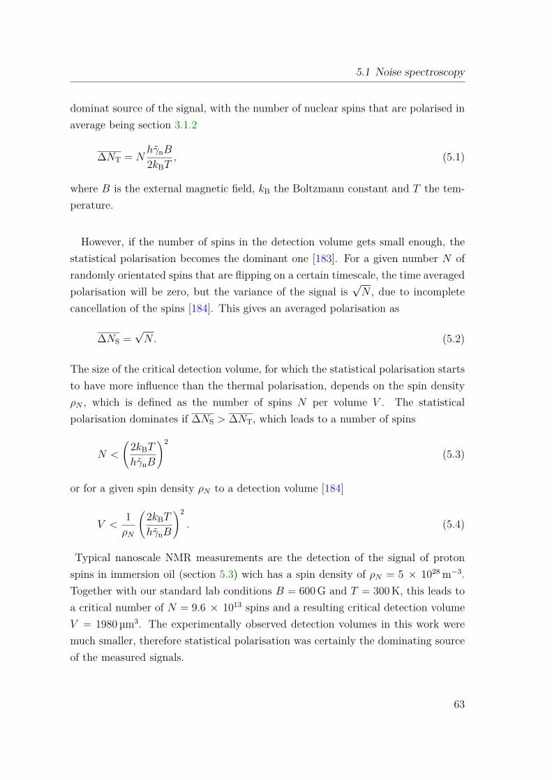
5.1 Noise spectroscopy
dominat source of the signal, with the number of nuclear spins that are polarised inaverage being section 3.1.2
∆NT = NhγnB
2kBT, (5.1)
where B is the external magnetic field, kB the Boltzmann constant and T the tem-perature.
However, if the number of spins in the detection volume gets small enough, thestatistical polarisation becomes the dominant one [183]. For a given number N ofrandomly orientated spins that are flipping on a certain timescale, the time averagedpolarisation will be zero, but the variance of the signal is
√N , due to incomplete
cancellation of the spins [184]. This gives an averaged polarisation as
∆NS =√N. (5.2)
The size of the critical detection volume, for which the statistical polarisation startsto have more influence than the thermal polarisation, depends on the spin densityρN , which is defined as the number of spins N per volume V . The statisticalpolarisation dominates if ∆NS > ∆NT, which leads to a number of spins
N <
(2kBT
hγnB
)2
(5.3)
or for a given spin density ρN to a detection volume [184]
V <1ρN
(2kBT
hγnB
)2
. (5.4)
Typical nanoscale NMR measurements are the detection of the signal of protonspins in immersion oil (section 5.3) wich has a spin density of ρN = 5 × 1028 m−3.Together with our standard lab conditions B = 600G and T = 300K, this leads toa critical number of N = 9.6 × 10¹³ spins and a resulting critical detection volumeV = 1980 µm3. The experimentally observed detection volumes in this work weremuch smaller, therefore statistical polarisation was certainly the dominating sourceof the measured signals.
63

5 Sensing of External Spins
time
noise
1Figure 5.2: Magnetic field from statistically polarised spins. The oscillating magneticfield generated by the precession of statistically polarised spins in an external magnetic field isstatistically varying in phase and amplitude with a frequency centred around the characteristicLarmor frequency.
As in conventional NMR, if there is an external magnetic field applied, the mag-netic moments of the nuclear spins will precess around the magnetic field axis withtheir Larmor frequency νL. While the phase and amplitude of the resulting ac mag-netic field will vary statistically, the frequency remains centred around the charcter-istic Larmor frequency of the respective nuclei (figure 5.2).
5.1.2 XY8 sensing
One experimental method to detect the resulting small ac magnetic fields is noisespectroscopy with the XY8 sequence. As already discussed in section 2.3.6, theperiodic refocussing pulses in the XY8 sequence are leading to an improved decoup-ling from high frequency fluctuations in the NV centre’s surrounding. This worksfor most frequencies, but becomes very inefficient for frequencies, where consecutivezero-crossings coincide with the π-pulses of the sequence. Instead of cancellation ofthe noise, it then leads to an accumulation. This effect is illustrated in figure 5.3,where the first line shows a train of π-pulses as in the case of a CPMG or XY8sequence. The second line of the figure represents an ac magnetic field Bac with afrequency ν. If the condition ν = 1/2τ is fulfilled, the flipping of the NV spin is inresonance with Bac and for an observer sitting on the NV axis, the external field isoriented into the same direction for the whole time (last line of figure 5.3). As inthis case the decoupling effect of the XY8 sequence is not working any more, thecoherence of the NV spin is lost, and for τ = 1/2ν a signal can be observed. To be
64

5.1 Noise spectroscopy
π π π π π π π π
τ τ τ τ τ τ τ
ν = 1/2τ
XY8-N
Bac
Bac @ NV
1Figure 5.3: Noise spectroscopy with the XY8 sequence. If the spacing τ between theπ-pulses of the XY8 sequence and the frequency ν of an oscillating magnetic field Bac fulfillthe condition ν = 1/2τ , this leads to an accumulation of noise rather than a cancellation. Inthis way, one can tune the XY8 sequence to be sensitive to a desired frequency by changingthe spacing τ .
more precise, not only the condition τ = 1/2ν leads to decoherence, but in generalalso higher orders are possible, with their positions given by [39]:
τk = (2k − 1)2ν , with k = 1, 2, 3, ... (5.5)
In order to use the XY8 sequence for spectroscopy one needs to have the feature tomake it sensitive for different frequencies. This is achieved by changing the spacingτ between the π-pulses. While for spacings τ that fulfill equation 5.5, the spin noiseaccumulates, it is still cancelled out for other spacings. By comparing the signal forthe different τ values, a drop in the fluorescence signal is observed for the matchingspacings (figure 5.4).
As the π-pulses in the XY8 sequence have the form of square-shaped pulses withfinite length instead of the theoretically assumed δ-peaks, the real measurementsmay show even more features than the above mentioned peaks at odd multiplesof the expected value of τ . Phase accumulation during the π-pulses itself leadsto signals even at shorter spacings τk/2, τk/4 and τk/8 [185]. This easily leads tomissinterpretation of signals, for example in the case of distinguishing 1H and 13Cnuclei, since the gyromagnetic ratio of hydrogen γ1H = 42.58 kHz/mT is roughly thesame as four times the gyromagnetic ratio of carbon 4 · γ13C = 42.82 kHz/mT [185].
65

5 Sensing of External Spins
spacing τ
flu
ores
cen
ce(n
orm
.)
τ = 1/2ν
1Figure 5.4: Typical signal for XY8 sensing. Sensing of external spin noise of statisticallypolarised spins with a given frequency ν leads to a lost of coherence for values of the spacingτ that fulfill the condition τ = 1/2ν.
5.1.3 The filter function
When applying the XY8 sequence, the detected signal, which appears as a dropin the fluorescene, is again depending on a phase that is picked up during themeasurement. In the case of statistical spin noise, the averaged random phase 〈ϕ2〉after many repetitions of the sequence is of interest. It is given by [186]
⟨ϕ2⟩
= γ2NVπ
∞∫−∞
S(ω)F (ωt)ω2 dω, (5.6)
where S(ω) is the power spectral density of the magnetic field signal [61]
S(ω) =∞∫−∞
〈B(t)B(0)〉 eiωtdt (5.7)
and F (ωt) is the filter function obtained by the application of the XY8 sequence.The filter-function has the form [186, 187]
F (ωt) = sin4(ωt
4N
)sin2
(ωt
2
)/ cos2
(ωt
2N
), (5.8)
where ω = 2πν and t = Nτ is the total length of the decoupling sequence. Whilethe frequency on which the XY8 sequence is most sensitive is given by the spacingτ between the π-pulses, it is the total length t of the decoupling sequence thatdetermines the linewidth at a given frequency ν.
66
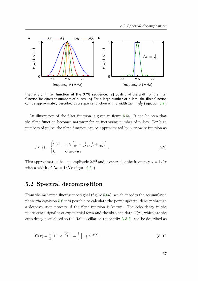
5.2 Spectral decomposition
2.4 2.5 2.60
1
frequency ν (MHz)
F(ω
)(norm.)
32 64 128 256
2.4 2.5 2.60
1
frequency ν (MHz)
F(ω
)(norm.)
a b
∆ν = 1Nτ
1Figure 5.5: Filter function of the XY8 sequence. a) Scaling of the width of the filterfunction for different numbers of pulses. b) For a large number of pulses, the filter functioncan be approximately described as a stepwise function with a width ∆ν = 1
Nτ (equation 5.9).
An illustration of the filter function is given in figure 5.5a. It can be seen thatthe filter function becomes narrower for an increasing number of pulses. For highnumbers of pulses the filter-function can be approximated by a stepwise function as
F (ωt) =
2N2, ν ∈[
12τ −
12Nτ ,
12τ + 1
2Nτ
]0, otherwise
. (5.9)
This approximation has an amplitude 2N2 and is centred at the frequency ν = 1/2τwith a width of ∆ν = 1/Nτ (figure 5.5b).
5.2 Spectral decomposition
From the measured fluorescence signal (figure 5.6a), which encodes the accumulatedphase via equation 5.6 it is possible to calculate the power spectral density througha deconvolution process, if the filter function is known. The echo decay in thefluorescence signal is of exponential form and the obtained data C(τ), which are theecho decay normalized to the Rabi oscillation (appendix A.3.2), can be described as
C(τ) = 12
[1 + e−
〈ϕ2〉2
]= 1
2[1 + e−χ(τ)
]. (5.10)
67

5 Sensing of External Spins
spacing τ
flu
ores
cen
ce(n
orm
.)
frequency ν
S(ω
)(n
orm
.)
a b
deconvolution
τ = 1/2ν ν = 1/2τ
1Figure 5.6: Signal reconstruction by deconvolution. If the filter function of the appliedsequence is known, the power spectral density S(ω) can be obtained from the measuredfluorescence data by a deconvolution process.
The function χ(t) is then connected to our measured data C by
χ(τ) = − ln(2C(τ)− 1). (5.11)
Together with equation 5.6 this leads to the following definition for χ(τ):
χ(t) = γ2NV2π
∞∫−∞
S(ω)F (ωt)ω2 dω (5.12)
= γ2NVπ
∞∫0
S(ω)F (ωt)ω2 dω. (5.13)
By using the filter function approximation (equation 5.9) the formula simplifies to
χ(τ) = γ2NV
4π2NτS(ω) (5.14)
and therefore the power spectral density (figure 5.6b) can be calculated as1
S(ω) = 1γ2
NV
π2
41Nτ
χ(τ) (5.15)
with ω = π/τ .
1While this is the correct formula for the power spectral density, in the plots presented in thisthesis, whenever S(ω) is plotted, it is multiplied by γ2
NV, to have the power spectral density inunits of Hz, which is the more common presentation.
68

5.3 Detection of external hydrogen spins
5.3 Detection of external hydrogen spins
1
2
4
5
6
7
8
10
11 12
13
1415
16
17
1818
19
205µm
1Figure 5.7: Confocal image of sample 69. The confocal map of sample 69 shows all meas-ured NV centres. All labelled NV centres have the same orientation and are implanted withan energy of 2.5 keV.
The first sensing experiments we performed were aiming for the detection of ex-ternal hydrogen spins, similar to the work done by Staudacher et al. [46]. On theone hand, these experiments were an easy check that the detection of external spinsis possible with our samples and on the other hand they enabled the calculation ofthe depth of the NV centres out of the measured data, which was of importance forthe upcoming experiments.The samples we used were two 99.999% 12C enriched isotopically purified CVD
grown diamonds with an as-grown surface with (100) orientation, provided by Ele-ment 62. They were implanted with 3× 10⁸ 15N+ ions/cm2 with acceleration voltagesof 2.5 and 5 keV. According to the SRIM simulations shown in figure 2.16b, this cor-responds to NV centre depths between 2 and 7 nm and 5 to 13 nm, respectively.Following the convention used at our institute, those two almost identical samplesare referred to as sample 69 and sample 70 within the upcoming chapters. A confocalimage of the 2.5 keV implanted region of sample 69 is given in figure 5.7, where singleNV centres can be seen.
2www.e6.com
69

5 Sensing of External Spins
0.60 0.70 0.80
0.95
1.00
1.05
1.10
frequency ν (MHz)
flu
ores
cen
ce(a
.u.)
0.40 0.50 0.60 0.70
100
150
frequency ν (MHz)
mag
net
icfi
eld
(G)
a b
129 G 148 G 171 G1H: 4.258 kHz/G
1Figure 5.8: Magnetic field dependency of the hydrogen signal. a) The fluorescencesignal shows loss of coherence at certain frequencies (corresponding to certain spacings τ) fordifferent applied magnetic fields after applying an XY8-16 sequence. b) Plotting the appliedmagnetic field over the detected frequencies confirms that the signal has a slope correspondingto the gyromagnetic ratio of 1H (black line). The gray data points correspond to additionalmeasurements that are not shown in a). The measurements were performed on NV1 ofsample 69.
After the implantation process, the samples were annealed and subsequentlyboiled in tri-acid at 180C for several hours to remove surface contaminations andto improve the NV centre properties with the resulting oxygen termination (sec-tion 2.4.3).
The sample to be detected were the hydrogen spins contained in the immersion oil(Fluka Analytical 10976) itself, which has a proton density of 50 nm−3 [46]. As wewill see later, the sensing volume and therefore the number of spins contributing tothe NMR signal is comparatively small. For the shallowest NV centres, the numberof spins is in the order of 102 – 103. While their magnetisation is zero in average,they still show the above mentioned statistical polarisation of
√N , which generates
an ac magnetic field at the NV centre with the Larmor frequency of hydrogen andwhich can be detected with the XY8 sensing scheme.
For different external magnetic fields Bext between 100 and 200G, XY8-16 se-quences were applied. The spacings τ were chosen to cover a range around the expec-ted Larmor frequency of the hydrogen spins, which can be calculated as νL = γpBext
with γp = 4.258 kHz/G. The recorded fluorescence data show clearly visible dipsat the expected frequencies (figure 5.8a), which arise from loss of coherence due to
70

5.3 Detection of external hydrogen spins
0.70 0.75 0.80 0.85
0.95
1.00
1.05
frequency ν (MHz)
flu
ores
cen
ce(a
.u.)
XY8-16 XY8-32 XY8-64
0 5 10100
101
102
103
104
depth d (nm)
linew
idth
∆ν
(kH
z)
calculated experimenta b
1Figure 5.9: Linewidth of the hydrogen NMR signal. a) The linewidth ∆ν of the 2.4 nmdeep NV1 was not limited by the spectral resolution of the applied sequence, which is indicatedby the dashed lines. b) Measured linewidths ∆ν for NV centres in different depths comparedto the expected linewidth calculated by equation 5.16. For the NV centres deeper than 5 nmthe linewidth was limited by the XY8 sequence in this measurement.
the higher noise level. Note that the x-axis of the plot is in frequencies, which arecalculated by ν = 1/2τ .
When plotting the external magnetic field over the detected frequencies, it canbe seen that the frequencies are shifting as expected for the gyromagnetic ratio ofhydrogen (figure 5.8b). A linear fit gave a value of γp = 4.20 ± 0.06 kHz/G, whichfits very well to the literature value.
Another thing that is noticeable in figure 5.8a is the linewidth of the hydrogenNMR signal, which is about 100 kHz. To examine whether this broadening is due tothe spectral resolution of the applied sequence, the behaviour of the linewidth underdifferent decoupling sequences was investigated. These measurements are presentedin figure 5.9a. Three sequences with an increasing number of pulses and a resultinghigher spectral resolution were applied to detect the hydrogen NMR signal. Whilethe expected linewidth decreased from ∆ν = 95 kHz down to ∆ν = 24 kHz when wechanged from the XY8-16 sequence to the XY8-64 sequence, the linewidth of thesignal stayed the same. Reason for this comperatively broad linewidth is diffusionof the hydrogen spins through the detection volume of the NV centre. Fast diffusionthrough a small sensing volume is reducing the interaction time between the NVcentre and the individual nuclear spins, which in turn broadens the NMR linewidth.
71

5 Sensing of External Spins
The observed value of 100 kHz linewidth for a 2.4 nm deep NV centre fits well toother reported values, like 120 kHz for 1.9 nm depth by Loretz et al. [138] or around140 kHz for an NV centre shallower than 5 nm by Ohashi et al. [102].The immersion oil we used in our experiments had a viscosity η = 437mPa·s and
a density ρ = 1.09 g/ml3. Following a derivation given in Pham et al. [188] thisleads to a diffusion coefficient Doil = 0.46 nm2/µs and an expected linewidth that isquadratically dependent on the NV centre’s depth [188]:
∆ν = Doil
d2 (5.16)
Plotting this equation shows good agreement with the experimental data (figure 5.9b).It has to be noted, that the values for the NV centres deeper than 5 nm were limitedby the spectral resoultion in this measurement. Nevertheless, the shallowest NVcentres and the overall tendency fits very well to equation 5.16.
5.4 Identification of shallow NV centres
The next step was then to perform the spectral deconvolution process on the meas-ured data, to obtain exact values for the interaction strength between NV centreand the hydrogen nuclear spins. For the data in this section, the approximation ofa stepwise filter function (equation 5.9) was used to calculate the power spectraldensity.A full data set for the depth determination process consists of the fluorescence data
of an XY8 sequence (figure 5.10a) and the corresponding Rabi measurement (fig-ure 5.10b). The Rabi measurement is thereby used to normalise the fluorescencedata of the XY8 sequence (appendix A.3.2). After doing so, one gets the normal-ised data plotted in figure 5.10c, which show the full contrast between the brightms = 0 and the dark ms = −1 state. The two different curves are two XY-32 meas-urements on NV4 in sample 69, that differ in the very last MW pulse. While thegreen curve uses a π/2-pulse for the population mapping, the blue one uses a 3π/2pulse. This leads to a population inversion compared to the green curve.
3values given by Sigma-Aldrich Co., www.sigmaaldrich.com
72
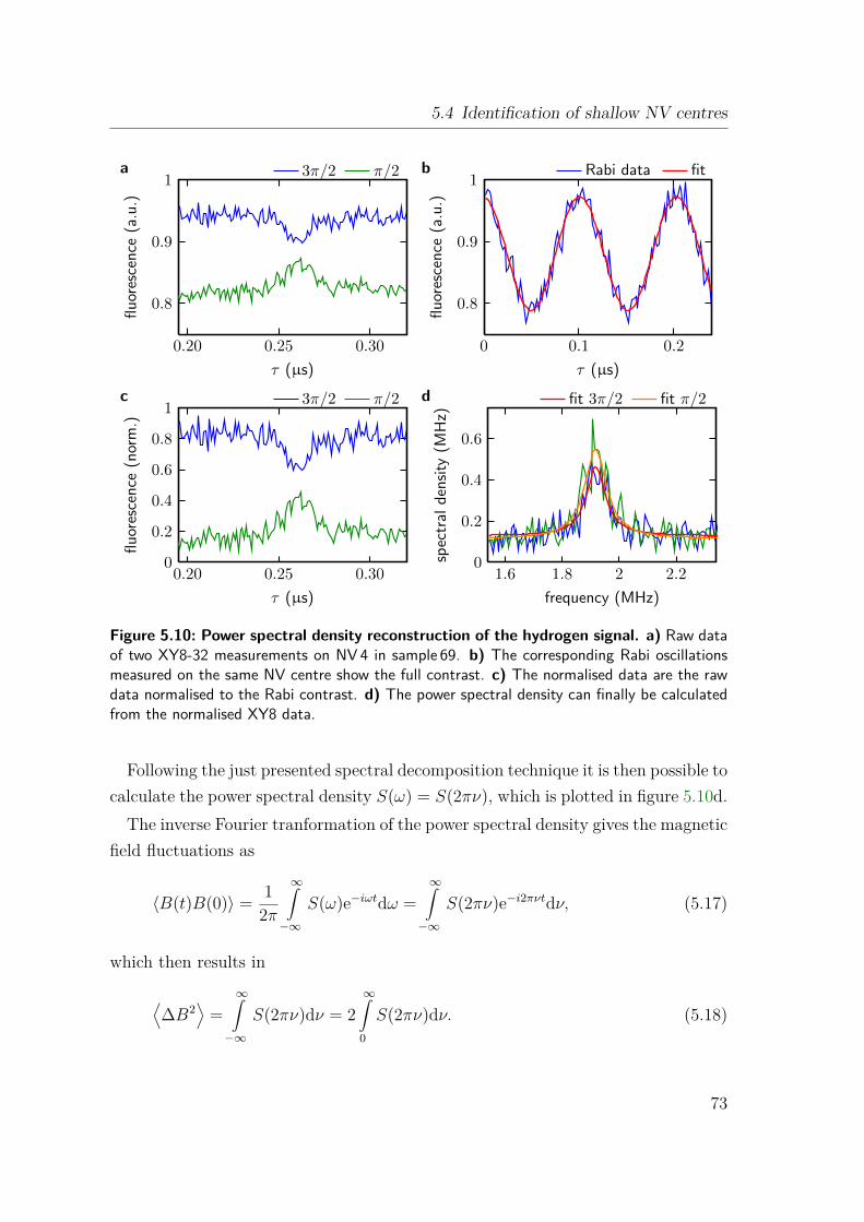
5.4 Identification of shallow NV centres
0 0.1 0.2
0.8
0.9
1
τ (µs)
flu
ores
cen
ce(a
.u.)
Rabi data fit
0.20 0.25 0.30
0.8
0.9
1
τ (µs)
flu
ores
cen
ce(a
.u.)
3π/2 π/2
0.20 0.25 0.300
0.2
0.4
0.6
0.8
1
τ (µs)
flu
ores
cen
ce(n
orm
.)
3π/2 π/2
1.6 1.8 2 2.20
0.2
0.4
0.6
frequency (MHz)
spec
tral
den
sity
(MH
z)
fit 3π/2 fit π/2
a b
c d
1Figure 5.10: Power spectral density reconstruction of the hydrogen signal. a) Raw dataof two XY8-32 measurements on NV4 in sample 69. b) The corresponding Rabi oscillationsmeasured on the same NV centre show the full contrast. c) The normalised data are the rawdata normalised to the Rabi contrast. d) The power spectral density can finally be calculatedfrom the normalised XY8 data.
Following the just presented spectral decomposition technique it is then possible tocalculate the power spectral density S(ω) = S(2πν), which is plotted in figure 5.10d.The inverse Fourier tranformation of the power spectral density gives the magnetic
field fluctuations as
〈B(t)B(0)〉 = 12π
∞∫−∞
S(ω)e−iωtdω =∞∫−∞
S(2πν)e−i2πνtdν, (5.17)
which then results in
⟨∆B2
⟩=
∞∫−∞
S(2πν)dν = 2∞∫0
S(2πν)dν. (5.18)
73

5 Sensing of External Spins
Therefore, the area below the peak centred at the Larmor frequency of the hydrogenspins corresponds to their magnetic field fluctuations. The value of the magneticfield fluctuation was then obtained by fitting a Lorentzian function of the form
L(A, ν,∆ν, ν0) = A
π
∆ν2
(ν − ν0)2 +(
∆ν2
)2 , (5.19)
where ∆ν is the linewidth, ν0 the centre of the peak and A the area below the peak.Together with equation 5.18 one gets for the magnetic field fluctuations
⟨∆B2
⟩= 2A. (5.20)
5.4.1 Depth calculation
The procedure of determining the depth of an NV centre out of the recorded XY8spectra will be shown in this section. As exemplary data set, the most shallowNV centre that was measured during our experiments is taken, which was NV6in sample 69. The normalised fluorescence data and the resulting power spectraldensity are plotted in figure 5.11a and figure 5.11b, respectively.The data were obtained by applying an XY8-16 sequence, for which the filter-
function has a linewidth of ∆ν = 312.5 kHz at ν = 2.5MHz. The Lorentzian fitgave a linewidth of ∆ν = 300 ± 30 kHz, so here the broadening results from thespectral resolution of the applied XY8 sequence.From the Lorentzian fit one gets the value of the magnetic field fluctuations,
which for this measurement was√〈∆B2〉 = 2.58 µT. By calculating the magnetic
field, that different proton spins would evoke at the position of the NV centre alongits axis and integrating that signal over the oil layer on top of the diamond, one getsa formula that connects the magnetic field fluctuations with the depth d of an NVcentre. This derivation is shown in the following.A single proton in a distance r from the NV centre, where r correspond to the
vector connecting the proton and the NV centre, evokes a magnetic field of the form
B(r) = µ0hγp
4πr3
[(3n2
z − 1)Iz + 3nz (nxIx + nyIy)
](5.21)
74

5.4 Identification of shallow NV centres
0.1 0.2 0.3
0.8
0.9
1.0
time τ (µs)
flu
ores
cen
ce(n
orm
.)
data
2.0 2.5 3.0
0.2
0.3
0.4
0.5
frequency ν (MHz)
S(ω
)(M
Hz)
data fita b
1Figure 5.11: Power spectral density reconstruction of the hydrogen signal of NV 6.a) The fluorescence data show a characteristic dip at the expected spacing τ = 1/2ν. b) Thepower spectral density is fitted by a Lorentzian function. The displayed results have previouslybeen published in [61].
with the nuclear spin operator ~I = (Ix, Iy, Iz)T , the direction cosines ni = ei · r andz-direction corresponds to the NV axis. The variance of this formula is given by
∆2B(r) =(µ0hγp
4πr3
)2 [(3n2
z − 1)2⟨(Iz)2
⟩+ 9n2
z
(n2x
⟨(Ix)2
⟩+ n2
y
⟨(Iy)2
⟩)]. (5.22)
Since the nuclear spins are randomly orientated in the sample, it can be assumedthat
⟨(Ii)2
⟩= 1
3s(s+ 1) = 14 , (5.23)
with s = 1/2 for hydrogen nuclear spins.
In the next step, the field fluctuation ∆2Bz(rk) is separated into its parts trans-versal and parallel to the NV axis, as
∆2B⊥(r) = 14
(µ0hγp
4πr3
)2 [9n2
z
(1− n2
z
)](5.24)
∆2B‖(r) = 14
(µ0hγp
4πr3
)2 [(3n2
z − 1)2]. (5.25)
75

5 Sensing of External Spins
0 5 10 15 201.8
1.9
2.0
2.1
2.2
sample thickness h (nm)
NVcentredepth
d(nm)
0 500 1,000 1,5000.0
0.5
1.0
1.5
2.0
number N of 1H spins
√〈∆
B2
(N)〉
(µT)
a b
1Figure 5.12: Depth and number of detected hydrogen spins of NV 6. a) Calculateddepth of the NV6 as a function of the sample thickness h. For thicknesses h > 10 nm thecalculated depth becomes independent from h. b) Simulation of the signal strength as afunction of hydrogen spins placed on top of the diamon surface. Around 390 – 400 spins madethe most significant contribution to the signal. This corresponds to in average 20 polarisedspins. The displayed results have previously been published in [61].
Integrating those two parts over the oil sample with its spin density ρN gives
∆2B⊥z = ρN(µ0hγp)2
64π2
π/2∫0
2π∫0
∞∫d/ cos θ
[9n2
z
(1− n2
z
)]r4 sin θdϕdrdθ (5.26)
∆2B‖z = ρN(µ0hγp)2
64π2
π/2∫0
2π∫0
∞∫d/ cos θ
[(3n2
z − 1)2]r4 sin θdϕdrdθ. (5.27)
With an NV axis tilted to the diamond surface normal by 54.7, which comes withthe (100) orientation of the sample, we have ez =
√13(1, 1, 1) and the solution of the
integrals becomes
∆2B⊥z = ρN (µ0hγp)2 51536π
[1d3 −
1(d+ h)3
](5.28)
∆2B‖z = ρN (µ0hγp)2 31536π
[1d3 −
1(d+ h)3
](5.29)
where d is the depth of the NV center and h the thickness of the sample attachedto the diamond surface.
76

5.4 Identification of shallow NV centres
NV1 NV6 NV7√〈∆B2〉 (µT) 2.39 2.58 2.23
depth (nm) 2.2 2.1 2.4
Table 5.1: Estimated NV centre depths. The estimated depths for the three shallowest NVcentres NV 1, NV6 and NV7. The results have previously been published in [61].
As only the transversal part of the field fluctuations contributes to the signalmeasured by the NV centre, the final solution is
√〈∆B2〉 =
√5
1536πµ0hγpρ1/2N
√1d3 −
1(d+ h)3 . (5.30)
In the case of the hydrogen spins in immersion oil, the thickness h is comparativelylarge and the term 1
(d+h)3 is negligible. This behaviour is shown in figure 5.12a,where the obtained value of d is plotted depending on the sample thickness h for themagnetic field fluctuation of 2.58µT measured on NV6. For thicknesses larger than10 nm the calculated depth is already independent from the thickness. Therefore,the final formula is
d =[
1〈∆B2〉
51536πµ
20h
2γ2pρN
]1/3
. (5.31)
This gave a depth of slightly more than 2.1 nm for NV6. Values for the two othermost shallow NV centres are given in table 5.1 and some more data on depths ofNV centres are presented in chapter 7.By comparing the measured signal with a simulation, where we placed proton spins
one after the other, thereby taking into account the spin density of the oil, on topof an NV centre in a depth of 2.1 nm and summed up their individual contributionsto the signal, we found that around 390 – 400 nuclei made the most significantcontribution to the signal (figure 5.12b). This means that the measured signal wasevoked by in average 20 polarised proton spins. Together with the spin densityof 50 nm−3 this led to a sensing volume of around (2 nm)3 above the diamond.Compared to the critical detection volume derived in section 5.1.1, this means thatwe are clearly in the domain of statistical polarisation.
77


6 Single Spin Sensing
NV
2.1 nm
1Figure 6.1: Sensing silicon nuclear spins. In this experiment, 29Si nuclear spins (orange andgray) were brought close to the diamond surface. For the closest nuclei (orange), the interactionbetween the NV centre and individual 29Si spins became stronger than the interactions betweenthe nuclei themselves and the strong coupling regime was reached.
While a number of only 20 polarised spins that contribute to the measured sig-nal, as presented in the previous chapter, is already close to ultimate sensitivity,the remaining goal was still to show single spin sensitivity. To achieve this goal,one needs to apply a new detetction scheme. By making use of the strong coulpingregime (section 6.2), where the interaction between the NV centre and individualnuclei dominates over all other interactions, it is possible to detect completely un-polarised nuclei. The strong coupling regime was reached by bringing 29Si nuclearspins close enough to the NV centre (figure 6.1).In the first experiment the nuclei were identified to be silicon by observing the
shift of the signal peak when the magnetic field was changed (section 6.1), as shownfor hydrogen nuclear spins in the previous chapter. This and the following measure-ments were performed in cooperation with Liam McGuinness and Xi Kong.The NV centre itself induced a magnetic field gradient at the position of the 29Si
nuclei, leading to an inhomogeneous broadening of the detected signal. By using
79

6 Single Spin Sensing
basis pursuit de-noising [189], a method closely related to compressed sensing, it waspossible to locate individual 29Si nuclei with sub-nanometre precision (section 6.3).The basis pursuit de-noising calculations were performed by Prof.Martin Plenio1
and Jianming Cai1.In the last part of the chapter it is shown that the achieved signal-to-noise ratio is
in principle sufficient to allow the detection of a single nuclear spin under ambientconditions within a few seconds (section 6.4). Thus, the presented experimentsare a further important step towards non-invasive and non-destructive imaging ofsingle nuclei and molecules under ambient conditions, overcoming the restriction onensemble averaged data.The results presented in this chapter have previously been published in [61].
6.1 Sample preparation and characterisation
The experiments were carried out on the same sample as the hydrogen sensing ex-periments presented in the previous chapter. That means on a 99.999% 12C enrichedisotopically purified CVD grown diamonds with an as-grown surface with (100) ori-entation, provided by Element 6. More precisely, we chose the previously mentionedNV6 (figure 5.7), which was implanted with an acceleration voltages of 2.5 keV andfrom which we exactly knew the depth of d = 2.1nm from the measurements of thehydrogen nuclear spin signal.After the hydrogen measurements, the diamond was cleaned in a 1:1:1 mixture of
sulfuric (H2SO4), perchloric (HClO4) and nitric (HNO3) acid at 180C for severalhours. The 29Si spins were brought to the diamond surface by dropping ∼ 10 µlof a 1:1 solution of (tetraethyl orthosilicate:ethanol) onto the diamond and sub-sequently heating it on a hotplate at 180C for 10min. After the heating process,an amorphous silica layer (SiO2) was left on the surface.
6.1.1 Detection of external silicon spins
Before performing further experiments it had to be made sure that the 29Si spinswere properly attached to the diamond’s surface. To do so, XY8 sequences withspacings τ matching to the Larmor frequency of 29Si were run. As we were working at
1Institute for Theoretical Physics, University of Ulm
80

6.1 Sample preparation and characterisation
1.60 1.65 1.70 1.75
0.65
0.70
0.75
0.80
0.85
frequency (MHz)
flu
ores
cen
ce(a
.u.)
1.60 1.65 1.70 1.75
0.19
0.20
0.21
frequency (MHz)
mag
net
icfi
eld
(T)
a b
1894 G 1951 G 1993 G 2044 G29Si: 0.847 kHz/G
1Figure 6.2: Magnetic field dependency of the silicon signal. a) Measurements of the 29Sisignal at different magnetic fields. The blue, red and orange signals were obtained by XY8-64,whereas for the green signal XY8-128 was used. It can clearly be seen how a higher numberof pulses narrows the signal. b) Plotting the Larmor frequency as a function of the magneticfield shows that the signal has a slope corresponding to the gyromagnetic ratio of 29Si (blackline). The grey data points correspond to additional measurements that are not shown in a).The displayed results have previously been published in [61].
magnetic fields around B = 2000G, the corresponding Larmor frequency was νL =|γSi|B ≈ 1.69MHz with γSi = −0.847 kHz/G. The measurements were repeatedat slightly varying magnetic fields and a matching shift of the signal peak wasobserved (figure 6.2a). For the measurements at 1894G, 1951G and 2044G anXY8-64 sequence was used and an XY8-128 sequence at 1993G. That explains thenarrower signal for 1993G, since the linewidth shrinks with longer sequences, andthe lower fluorescence level, which comes along with longer total waiting time andtherefore decreased coherence.
Again, the obtained Larmor frequencies were plotted as a function of the externalmagnetic field (figure 6.2b). A linear fit gave a value of γSi = 0.859 ± 0.012 kHz/Gwhich is in good agreement with the values reported in literature. It should benoted that for measurements without silica sample, there was no measurable signalobtained at the same spacings on the same NV centre. In this way it was verifiedthat the signal is evoked by the silicon spins and not by the 1/5 harmonic of the 1Hsignal, which would give 0.851 kHz/G [185].
81

6 Single Spin Sensing
6.2 Strong coupling regime
As already explained in chapter 3, the sensitivity in classical NMR is restrictedby low thermal polarisation and inductive detection. The interaction ΓN betweensample spins is much larger than the interaction ΓS between individual spins andthe sensor. Here, the time averaged signal 〈S〉 is proportional to the thermal polar-isation (figure 6.3a).
By going to nanoscale detection volumes, one reaches the regime of statisticalpolarisation (section 5.1.1). In this regime, the interaction between the spins itselfis still larger than the interaction between spin and sensor. However, the polarisationis not thermal any more, but statistical and the signal is proportional to
√N with
N being the number of sample spins in the detection volume (figure 6.3b).
The strong coupling regime is reached, when the interaction strength betweensensor and spins exceeds the interaction between individual spins (ΓS > ΓN). Thesensitivity is then directly proportional to the number of strongly coupled spins (fig-ure 6.3c). To reach this regime, silica was chosen as sample, because most of thesilicon atoms are free of nuclear spin. Only 4.67% of the silicon atoms are of type29Si, which is the only stable isotope of silicon carrying a nuclear spin (I = 1/2).This gave a spin density of 1 spin nm−3, which shows that the silicon spins are ratherdiluted compared to the hydrogen spins in the previous experiment and fewer spinsare present in the detection volume.
In SiO2, the shortest distance between two silicon atoms is 0.306 nm and theresulting coupling is 0.17 kHz. This coupling is smaller than the coupling betweenan NV centre and a silicon spin with a separation of 2.1 nm, which is ∼ 3 kHz. Thus,ΓS > ΓN is fulfilled and the strong coupling regime is reached in our experiments.
The hyperfine interaction between an NV centre and a 29Si nuclear spin at alocation (x,y,z) in distance r can be described by the Hamiltonian
H = νLIz + µ0γNVγSih2
4πr3 Sz (3nz [nxIx + nyIy + nzIz]− Iz) , (6.1)
where the second term can be rewritten as
µ0γNVγSih2
4πr3 Sz(Iz(3 cos2 θ − 1
)+ 3nz [nxIx + nyIy]
)(6.2)
82

6.2 Strong coupling regime
ΓS
ΓN
NV
ΓS
ΓN
NV
ΓS
ΓN
a Classical NMR b Statistical fluctuations c Strong coupling
ΓS < ΓN ΓS < ΓN ΓS > ΓN
〈S〉 ∝ N↓ −N↑ 〈S〉 ∝√N 〈S〉 ∝ N
1Figure 6.3: The three different sensing regimes. a) In classical NMR, the interaction ΓSbetween sensor and individual spins is much weaker than the interaction ΓN between individualnuclei and the time averaged signal 〈S〉 is proportional to the thermal polarisation. b) In theregime of statistical polarisation, we still have ΓS < ΓN, but the signal is now proportional to√N with N being the number of spins in the detection volume. c) In the strong coupling ΓN
is larger than ΓS and the signal is now directly proportional to the number N of spins in thedetection voulme.
with θ being the angle between the z-axis and the vector that connects the NVcentre and the nuclear spin. The first term gives the parallel and the second termthe perpendicular component of the hyperfine interaction.
Since the interaction between individual 29Si nuclear spins is much weaker than theinteraction beween NV centre and 29Si nuclear spins, we can neglect it (figure 6.4a).By defining I⊥,n ≡ (Ix, Iy) and summing over N nuclear spins, we then get
H = νL
N∑n
Iz,n + SzN∑n
(α‖,nIz,n + α⊥,n · I⊥,n
), (6.3)
where α‖,n and α⊥,n are the parallel and the perpendicular components of the hy-perfine coupling and in our experiments νL α‖,n, α⊥,n. Depending on the spinstate of the NV centre, which is either ms = 0 or ms = −1, the Hamiltonian is
H0 = νL
N∑n
Iz,n or (6.4)
H−1 = νL
N∑n
Iz,n −N∑n
(α‖,nIz,n + α⊥,n · I⊥,n
). (6.5)
83

6 Single Spin Sensing
1.725 1.730 1.735 1.740 1.745
0.4
0.6
0.8
1
Larmor frequency (MHz)
WSi
with Si-Si without Si-Si
−200 0 200
0.90
0.95
1.00
frequency (kHz)
sign
al
completely polarised unpolariseda b
XY8-512
d = 2.1 nm
4 nm deep NV
2 nm deep NV
1Figure 6.4: Simulations of the expected echo decay. a) The calculated echo decayWSi fora XY8-512 sequence on a 2.1 nm deep NV centre. The blue curve is including Si-Si interaction,whereas the red curve is not including them. It can be seen that in our experimental conditionsthe Si-Si interactions are negligible. b) Numerical simulation of the signal from 50 compeltelypolarised (red) and completely unpolarised (blue) 29Si nuclear spins for a XY8-512 sequenceon a 2 nm and on a 4 nm deep NV centre. The displayed results have previously been publishedin [61].
This means that in the case of ms = 0, there is no hyperfine interaction betweenthe NV centre and the 29Si nuclear spins, but if the NV centre is in the statems = −1,then each nuclear spin rotates around an axis defined by its local magnetic field.This local field is given by the vector sum of the external magnetic field and thelocal hyperfine field. By adjusting the NV spin repetitively, in synchrony with therotation of the nuclear spin, one can achieve a complete flip of the nuclear spintogether with a flop of the NV centre. The rotation rate is thereby given by thehyperfine component α⊥,n and the optimum timing depends on the component α‖,nand is matched with a spacing [39, 40]
τk = (2k − 1)2(νL + α‖,n/2π
) (6.6)
= (2k − 1) πω + α‖,n
, with k = 1, 2, 3, ... (6.7)
between the π-pulses of the XY8 sequence. The rotation occurs for every stronglycoupled 29Si nuclear spin, independent from its initial state (figure 6.4b) and forshort interaction times the overall signal of several nuclear spins approximates alinear sum of the individual contributions, leading to 〈S〉 ∝ N .
84

6.3 Resolving the position of individual nuclei
6.3 Resolving the position of individual nuclei
1.730 1.735 1.740 1.745
0.45
0.50
frequency (MHz)fl
uor
esce
nce
sign
al
a b
2.1 nm
1Figure 6.5: Inhomogeneous broadening of the silicon signal. a) Hyperfine interactionsbetween a shallow NV centre and nearby 29Si nuclear spins are distance dependent and areleading to an effective magnetic gradient experienced by the nuclear spins. b) Inhomogen-eous broadening of the 29Si signal. The experimental data (black) show an inhomogeneousbroadening (red, 10 kHz, obtained by basis pursuit de-noising) that is larger than the expectedlinewidth of the XY8-512 sequence (blue, 6 kHz). The displayed results have previously beenpublished in [61].
With the aim to resolve the hyperfine couplings of individual 29Si nuclei, thenumber of decoupling pulses in the XY8-N sequence was increased to N = 512pulses. This leads to a better spectral resolution. For large spin baths, as presentin the hydrogen measurements, the signal obtained by the XY8 sequence is centredaround the Larmor frequency with a width ∆ν = 1/Nτ . However, in the case ofstrong coupling, the individual nuclear spins are detuned due to the field gradientcreated by the NV centre itself (figure 6.5a, equation 6.7). At a distance of 2.1 nmfrom the NV centre, the field gradient is around 0.5G/nm. The resulting slightlydifferent fields for the individual nuclei led to an imhomogeneous broadening of thedetected signal (figure 6.5b), which offered a new opportunity for nanoscale imaging.By using advanced methods from signal processing, it was possible to exctract thefrequencies and the contributions to the signal of the individual nuclei out of theinhomogeneous broadened signal peak. This allowed to obtain the values α‖,n andα⊥,n from which further information on the position of the NV centres was gained.The chosen method for signal processing was basis pursuit de-noising [189], a methodsimilar to compressed sensing [190, 191].
85

6 Single Spin Sensing
6.3.1 Basis pursuit de-noising
To analyse the data of the silicon measurement, we first separated the contributionsto the echo decay from 29Si and from the background noise as
χ(τ) = χSi(τ) + χbg(τ) (6.8)
which gives the detected signal as
C(τ) = 12[1 + e−χSi(τ) + e−χbg(τ)
]. (6.9)
In the otained data, the background noise gives the overall decay for increasinginteraction time and the dip in the signal at the Larmor frequency is arising from thecontribution of the 29Si nuclei. The background decay was measured (figure 6.6a)and the power spectral density of the background was extracted by using the de-convolution process described in the previous chapter (figure 6.6b). Calculating anexpected decay out of the obtained power spectral density gave good agreementwith the experimental data (figure 6.6a). The measurements of the backgrounditself thereby gave us knowledge of χbg(τ).
The basis pursuit de-noising (BPDN) technique is an approximation techniquesimilar to compressed sensing, which determines a representation of the signal outof a large set of signal forms in an overcomplete dictionary [189]. The signal wewant to reproduce is the measured echo decay Cexp(τ), which depends on χ(τ). Weknow the contribution of the background χbg(τ) to the signal, and the contributionof the 29Si nuclei is actually the sum of the contributions of each individual nuclei.So we can write
χ(τ) =N∑n
χ(n)Si (τ) + χbg(τ). (6.10)
For the basis pursuit analysis it is assumed that each individual 29Si nuclei gen-erates a magentic field with a delta frequency at the effective Larmor frequency νn,
86

6.3 Resolving the position of individual nuclei
0.1 0.2 0.3 0.4 0.5
0.6
0.8
time τ (µs)
flu
ores
cen
ce(a
.u.)
data calculated
1 2 3 4 5
0.2
0.4
0.6
0.8
frequency ν (MHz)
S(ω
)(M
Hz)
dataa b
1Figure 6.6: Determination of the background noise spectrum. a) Measured signal decaydue to background noise (blue) and the calculated decay (red), which was reproduced fromthe deconvoluted power spectral density showed good agreement. b) The deconvoluted powerspectral density of the background noise. The displayed results have previously been publishedin [61].
and therefore the contribution of the individual nuclei to the signal takes the formof a normalised filter function, as
χ(n)Si (τ) = 4
K2 sin4(2πνnτ
4
)sin2
(2πνnKτ2
)/ cos2
(2πνnτ2
), (6.11)
where the number of pulses in the XY8 sequence is denoted as K, to avoid confusionwith N , which is used as the number of 29Si nuclei.
BPDN solves the problem to find a solution, that reproduces the experimentaldata Cexp(τ) up to a desired precision by using a superposition of the smallestnumber of given dictionary elements, which in our case would be the 29Si nuclearspins. To find the solution, the optimisation problem [61]
minbmax≥b≥012
∥∥∥∥∥∥∥∥12
1 + e−
J∑j=1
bjχ(j)Si
e−χbg(τ)
− Cexp
∥∥∥∥∥∥∥∥2
2
+ λJ∑j=1|bj| (6.12)
needs to be solved.
In this equation, the contribution of each basis function to the signal is quantifiedby bj, which can be identified with the perpendicular component of the hyperfinecoupling by a scaling factor. The value bmax is the maximal possible value for bj for
87

6 Single Spin Sensing
1.730 1.735 1.740 1.745
0.45
0.50
frequency (MHz)
flu
ores
cen
cesi
gnal
λ = 0.0001 λ = 0.0005 λ = 0.001
0 10 20 300
0.2
0.4
0.6
0.8
1
number of spins
sign
alco
ntr
ibu
tion
a b
1Figure 6.7: Signal contribution of individual spins. a) The fits obtained by BPDN remainedstable when changing the accuracy parameter λ. b) The contribution of up to 30 nuclear spinsto the echo signal, obtained by BPDN. Around 6 – 7 nuclear spins make the most significantcontribution (>70%). The displayed results have previously been published in [61].
an NV centre depth of 2.1 nm and λ determines how well the fitting data shouldagree with the experimental data. The number of basis functions is given by J andis set to J = 30, which means that 30 spins are taken into account to describe theexperimental signal. With the given density of the 29Si nuclei, this corresponds to asensing volume of ∼ 25 – 30 nm3. Since spins that are further away are not in thestrong coupling regime anymore, a number of 30 spins was sufficient to reproducethe signal successfully.
Good agreement with the experimental data was achieved with the BPDN tech-nique. The fit and the estimated number of contributing 29Si spins obtained fromBPDN remained stable when chanching the accuracy value λ (figure 6.7a).
Summing up the contribution of the 30 individual 29Si nuclear spins to the experi-mental signal in descending order, we find that 6 – 7 spins make the most significantcontribution (>70%) to the signal (figure 6.7b).
Not only the contribution of the individual nuclear spins, but also their effectiveLarmor frequencies were extracted from the measured data by the BPDN technique.The obtained signal contribution per nuclear spin together with the effective Larmorfrequency is plotted in figure 6.8a and the four spins with the strongest contributionto the signal are highlighted. These four spins contributed to more than 50% ofthe measured signal. BPDN thereby allows to recover frequency components with a
88

6.3 Resolving the position of individual nuclei
1.7365 1.7370 1.7375 1.73800
0.1
0.2
effective Larmor frequency (MHz)
sign
alco
ntr
ibu
tion
0 10 20 300
0.1
0.2
spin number
sign
alco
ntr
ibu
tion
a b
1Figure 6.8: Contributions of the four strongest contributing spins. a) Larmor frequencyand contribution of the 30 nuclear spins. The four spins with strongest contribution arehighlited. These four spins make already more than 50% of the total contribution. b) Thecontribution of the individual spins in descending order. The displayed results have previouslybeen published in [61].
higher resolution than the linewidth of the measured data. The stability of BPDNin presence of noise has been demonstrated mathematically [192].
With the data obtained from BPDN it was then possible to gain information aboutthe position of the 29Si nuclear spins with respect to the NV centre. As seen before,the parallel hyperfine component α‖ is causing a frequency shift of the signal andcan therefore be obtained from the value of the effective Larmor frequency and theperpendicular component α⊥ describes the coupling strength and can be obtainedfrom the signal contribution of the individual nuclear spins. By using equation 6.2together with equation 6.3 we get
α‖ = µ0γNVγSih2
4πr3
(3 cos2 θ − 1
)(6.13)
and
α⊥ = µ0γNVγSih2
4πr3 3 cos θ sin θ (6.14)
for the two components of the hyperfine interaction.
89

6 Single Spin Sensing
0
-1
-2-2
02
2 0 -2
x (nm)
y (nm)
z(nm)
silica
diamond
1Figure 6.9: Positions of the four strongest contributing spins. Best fit locations forthe four spins highlighted in figure 6.8. The displayed results have previously been publishedin [61].
Rearranging those two equations leads to [193, 194]
θ = arctan
12
−3 α‖α⊥
+
√√√√9α2‖
α2⊥
+ 8
(6.15)
and
r =[µ0γNVγSih
2
4πα‖
(3 cos2 θ − 1
)]1/3
. (6.16)
Knowing θ and r allowed to estimate the location of a nuclear spin up to onedegree of circular symmetry. The best fit locations for the four spins highlightedin figure 6.8a are indicated in figure 6.9. Uncertainties in the amplitude and fre-quency obtained from BPDN led to uncertainties in the position of the nuclei. Thesize of the balls that give the position of the nuclei in figure 6.9 corresponds tothe uncertainty in position. For the closest spin, the uncertainty was ∆x = 0.1nmand ∆z = 0.02nm and for the fourth closest spin we found ∆x = 0.15nm and∆z = 0.1nm. However, the azimuthal angle of the spins is unknown and they canbe positioned somewhere on the arcs of the same colours.Longer data acquisition times can lower down the uncertainties to below an Ång-
strom and by measuring at different orientations of the external field one can gainadditional information on the azimuthal angle. A longer acquisition time corres-ponds to a longer coherence time of the NV centres. This might be achieved by
90

6.4 Single nuclear spin sensitivity
1.718 1.722 1.726 1.730
0
0.5
1
Larmor frequency (MHz)
Eff
ecti
veN
MR
sign
al
100 s single spin
1.718 1.722 1.726 1.730
0
0.5
1
Larmor frequency (MHz)
Eff
ecti
veN
MR
sign
al
10 s single spina b
2σ
2σ
1Figure 6.10: Single spin sensitivity. a) The expected signal of a single 29Si nuclear spinpositioned at the gray surface given in figure 6.9 is compared to the noise level after 100 s ofacquisition time. The signal is well above two standard deviations. b) Even after only 10 sof acquisition time, the signal already exceeds two standard deviations. The displayed resultshave previously been published in [61].
better decoupling of unwanted noise sources. In order to find good performingdecoupling sequences, it is of importance to have a good knowledge of the noisesources in the NV centres’ environment. This noise sources for shallow NV centresare further investigated in chapter 7.
6.4 Single nuclear spin sensitivity
The obtained signal-to-noise ratio reaches single nuclear spin sensitivity – the ulti-mate sensitivity limit of NMR spectroscopy. To verify that, we measured the noiselevel after 10 s of measurement time for a single point and after 100 s and comparedthe noise level of the signal to the expected signal of a single strong coupled nuclearspin. It can be seen that the signal readily exceeds the shot noise by two standarddeviation values for the 100 s measurements (figure 6.10a) and is still well above thatvalue for only 10 s of single point measurement time (figure 6.10b).Further improvements in measurement time can be achieved by other signal pro-
cessing methods as compressed sensing that allow a reduction in the number ofrequired data points [195, 196].
91


7 Spectroscopy of Surface-InducedNoise
NV NV
1Figure 7.1: Surface spins affecting the NV centres. In this experiment, shallow NV centresin diamond are used as sensors to measure surface noise effects. The NV centres are therebyinteracting with fluctuating electronic spins (orange) on the diamond surface.
In the previous chapters we showed the exceptional capabilities of shallow NVcentres in terms of nanoscale magnetic resonance spectroscopy. New techniques,as sensing in the strong coupling regime, enable single nuclear spin sensitivity andcould have high impact in natural sciences. The main restriction on sensitivityand resolution are the coherence properties of shallow NV centres. In general theircoherence times are much worse compared to the values measured for NV centres inbulk diamond and they experience a strong dependence on the actual depth for veryshallow NV centres [142, 143]. However, the best for nanoscale NMR would be tohave a very shallow NV centre with a very long coherence time, since the minimumdetectable magnetic dipole moment µmin scales as µmin ∝ r3/
√T2 [143], where r is
the distance between the NV centre and the spin to be detected.Main noise sources for NV centres in bulk diamond are interactions with phon-
ons and internal nuclear and electronic spin baths [103, 187]. For very shallow NVcentres, there are additional noise sources on the diamond surface, that are drastic-ally shortening their coherence times (figure 7.1). Therefore, a better knowledge and
93

7 Spectroscopy of Surface-Induced Noise
understanding of these noise sources may help to improve the NV centres’ coherenceproperties. To measure the surface effects, we thereby used the shallow NV centresthemselves.First, the depths of the NV centres and their coherence times T2 were meas-
ured (section 7.1). The depth was accurately determined by detecting the protonNMR signal as shown in chapter 5. A strong dependence of the coherence time onthe depth was found for the shallowest NV centres. After that we applied differentCPMG sequences with increasing number of pulses to investigate the scaling of thecoherence time with the number of pulses for different depths and to show successfuldecoupling from the surface noise (section 7.2).Then, the noise spectra for the different NV centres were extracted out of the
measured echo decay data by spectral decomposition [197] (section 7.3), a techniquethat was also successfully used in other systems as for example in SQUIDs [198]. Theobtained noise spectra were further investigated and revealed a double-Lorentzianshape, which we interpret as a combination of a low frequency electronic spin bathand a faster noise source arising from a phonon-related relaxation mechanism (sec-tion 7.4).The experiments were performed together with Yoav Romach1 and Thomas Unden
and analysed with additional help from Nir Bar-Gill1. Parts of the results presentedin this chapter have previously been published in [141].
7.1 Sample characterisation
The measurements were carried out on several NV centres in sample 69 (figure 7.2a)and sample 70 (figure 7.2b). More NV centres were investigated and showed similarresults, but only a selection of some of the measured NV centres is presented in thischapter. More details on the additionally measured NV centres can be found in thesupplementary information of [141].On the investigated samples, the 2.5 keV implanted region was chosen, which gave
us a depth distribution of the NV centres between 2 and 10 nm. The close proximityof the NV centres to the surface, together with the high purity of the diamondsample (99.999% 12C, N < 5ppb) results in NV centres with coherence properties
1Racah Institute of Physics, Center for Nanoscience and Nanotechnology, Hebrew University ofJerusalem
94

7.1 Sample characterisation
a b
5µm
2
3
20
6 5
9
1Figure 7.2: Confocal images of sample 69 and sample 70. The confocal images show theposition of the measured NV centres within the 2.5 keV implanted regions of sample 69 (a)and sample 70 (b).
that are dominated by surface effects. Since we are particularly interested in surfaceeffects here, this makes these NV centres the ideal candidates for our experiments.In a first step, the depths of different NV centres were determined by nanoscale
NMR signal measurements of the protons in the immersion oil (section 5.4). Wethen chose five NV centres with different depths between 2.4 and 8.7 nm plus oneNV centre that was a bit deeper with a depth of around 20 nm. The numbering ofthe NV centres is chosen in a way that the number matches the depth of the NVcentre, so for example the NV centre in a depth of 8.7 nm is referred to as NV9. Tohave the basic data of the NV centre, we additionally measured the T2 time usingHahn-echo (T2,HE). Both, the values for the depths and the T2,HE coherence times,can be found in table 7.1.All sequences were run twice, with a final π/2- and a final 3π/2-pulse, respect-
ively (figure 7.3a). The data were normalised as
Cnorm = Cπ/2 − C3π/2
Cπ/2 + C3π/2. (7.1)
and then fitted with a stretched exponential function
exp [− (τ/T2)p] , (7.2)
where the free parameter p was in the range between 1 – 3. This is consistent withan electronic spin bath descibed by a Lorentzian spectrum [187].
95

7 Spectroscopy of Surface-Induced Noise
0 10 20 30
0.8
0.9
1
T2,HE (µs)
flu
ores
cen
ce(a
.u.)
3π/2 π/2
0 5 10 15 200
20
40
60
depth (nm)
T2,H
E(µ
s)
a b
1Figure 7.3: Depth dependency of the coherence time. a) Experimental data for a Hahnecho measurement on NV4. All measurements were performed twice, with a final π/2-pulse(green) and a final 3π/2-pulse (blue) b) The coherence time (T2,HE) of very shallow NVcentres is strongly dependent on the depth of the NV centres.
Plotting the coherence time T2,HE over the depth of the individual NV centres (fig-ure 7.3b) shows a strong depth dependence for the coherence time of very shallowNV centres. While the shallowest NV centres in a depth of around 2 – 4 nm showedcoherence times of around 5 – 10µs, the 20 nm deep NV20 exhibited a much longercoherence time of around 50 µs. These results are consistent with similar stud-ies [142, 143] and already indicate a noise source on the diamond’s surface.
7.2 T2 scaling under CPMG dynamical decoupling
After knowing the single pulse coherence times T2,HE, we carried out multi-pulseCPMG measurements on the same NV centres and observed the scaling of T2 withthe number of pulses N .As an example, the signals from different CPMG measurements on NV3 are
plotted in figure 7.4a and are also compared to a T1 measurement on the same NVcentre. One can clearly see how an increasing number of decoupling pulses extendedthe coherence time.For NV2 the maximum coherence time T2,sat was measured to be 42± 12 µs and
was reached after 65 ± 30 pulses and for NV3 we got T2,sat = 64 ± 10 µs after109 ± 22 pulses (table 7.1). This proved that dynamical decoupling is effective atsurpressing environmental decoherence even for shallow NV centres and the coher-
96

7.2 T2 scaling under CPMG dynamical decoupling
NV number sample number depth (nm) T2,HE (µs) scaling coefficient k2 69 2.4± 0.1 7.3± 0.5 0.42± 0.043 69 2.8± 0.1 9.6± 0.5 0.40± 0.035 70 5.3± 0.3 20± 5.0 0.37± 0.106 70 6.0± 0.3 33± 3.0 0.30± 0.069 70 8.7± 0.3 45± 10 0.45± 0.1020 69 20± 5.0 51± 10 0.53± 0.06
Table 7.1: Properties of the measured NV centres. Coherence times T2,HE, depths andthe scaling coefficient k of the investigated NV centres that are labelled in figure 7.2. Theresults have previously been published in [141].
ence times of around 50µs for NV centres between 2 and 3 nm from the surface wererecord values at the date of the publication.
We then took a closer look at the scaling of T2. The values for increasing number ofdecoupling pulses are plotted for different NV centres in figure 7.4b. Before reachingsaturation, the scaling follows a power law as
T2(N) = T2,HE ·Nk (7.3)
with a scaling coefficient k. This scaling coefficient is connected to a spectrum ofclassical noise described as
S(ω) ∝ ω−β (7.4)
via [199]
k = β
β + 1 . (7.5)
In the case of Lorentzian spectrum as present for an electronic spin bath [200]
S(ω) = ∆2τc
π
11 + (ωτc)2 (7.6)
97

7 Spectroscopy of Surface-Induced Noise
10−2 101 104
0
0.5
1
τ (µs)
sign
al(norm.)
T2(1) T2(4) T2(64) T1
100 101 102 103100
101
102
103
number of pulses N
T2(µ
s)
NV 20 NV4 NV3 NV2a b
NV3
1Figure 7.4: Scaling of the coherence time with the number of decoupling pulses.a) Signal after different decoupling sequences on NV3. b) The coherence time T2 was extendedby applying an increasing number of decoupling pulses. Before reaching saturation the scalingfollows a power law as T2(N) = T2,HE · Nk. The displayed results have previously beenpublished in [141].
with an average coupling strength ∆ of the environment to the NV spin and acorrelation time τc of the environment, the value of k would become 2/3 (in thelimit of τc T2 [187]) and we would observe a scaling as
T2(N) ∝ N2/3. (7.7)
Indeed, such a behaviour was observed experimentally for bulk NV centres in thepresence of Lorentzian noise [114, 201].
For the NV centres in our study, only NV20 with a scaling factor of k = 0.53±0.06showed a behaviour close to the one expected for a simple Lorentzian spin bath. Theshallow NV centres however had lower values of k ∼= 0.3− 0.45 (table 7.1), which isa first hint of either a different noise source or a Lorentzian spin bath with shortercorrelation times, since in the case of τc T2 the decoupling of the CPMG sequencebecomes inefficient and the scaling approaches T2(N) ∝ N0 [187].
In order to gain more information, we compared the saturated coherence times T2,sat
with the relaxation times T1 of the individual NV centres (table 7.2). Both, T2,sat
and T1 are related to high frequency noise, which can not be cancelled out by the ap-plied high order decoupling sequences. For shallow NV centres (NV2, NV3, NV4)the ratio between T2,sat and T1 was ∼ 0.1 and for the deeper NV20 a ratio of 0.3 was
98

7.3 Spectral decomposition
NV number T2,sat (µs) T1(µs) T2,sat/T1
2 42± 12 430± 225 0.0983 64± 10 860± 200 0.0744 130± 70 960± 500 0.13520 900± 300 3000± 1000 0.300
Table 7.2: Saturated coherence times and relaxation times. Comparison of the saturatedcoherence times T2,sat and the relaxation times T1 of shallow (NV2, NV3, NV4) and a deepNV centre (NV20). The ratio T2,sat/T1 differs for both types of NV centres, indicating twodifferent noise sources. The results have previously been published in [141].
obtained, which is closer to the value of 0.5 expected for bulk NV centres [103]. Thesmaller ratio for shallow NV centres indicates that they experience a strong highfrequency noise that couples to both, relaxation processes (affecting T1) and deco-herence processes (affecting T2,sat). These measurements verified the assumption ofa noise source at the diamond surface that is different to the one experienced bybulk NV centres.
7.3 Spectral decomposition
By applying several CPMG sequences with differing spacing times τ and number ofpulses N it was possible to obtain noise spectra of the NV centres’ environment bya spectral decomposition process. During the decomposition process it was assumedthat for very high frequency noise the spectral function becomes zero. Starting atthe shortest values of τ (i. e. the highest frequency noise) and going backwards infrequency, each value is then calculated by using the known filter function (equa-tion 5.8) and substracting effects of higher harmonics of the already recovered highfrequency components [202].The obtained noise spectra for two shallow NV centres (NV2 and NV3) and one
deep NV centre (NV20) are plotted in figure 7.5. Different fit-functions were appliedto the data in order to find the best fitting one. We compared a single Lorentzian,a double Lorentzian and an 1/ω fit (figure 7.6) and found that a double Lorentzianfunction of the form
S(ω) =∑i=1,2
∆2i τc,i
π
11 + (ωτc,i)2 , (7.8)
99

7 Spectroscopy of Surface-Induced Noise
105 106 107102
103
104
105
106
ω (Hz)
S(ω
)(H
z)
NV 20 NV3 NV2
1Figure 7.5: Noise spectra for different NV centres. Noise spectra for two shallow NVcentres (NV2 and NV3) and one deep NV centre (NV 20) obtained by spectral decomposition.Solid lines are fits using a double Lorentzian fit-function. The displayed results have previouslybeen published in [141].
105 106 107
103
104
105
106
ω (Hz)
S(ω
)(H
z)
data 2 Lorentzian fit 1 Lorentzian fit 1/ω fit
1Figure 7.6: Comparison of different fit-functions. Different fits to the data obtainedfrom NV3, using a double Lorentian (red), a single Lorentzian (green) and a 1/ω (blue) fit-function. Best fits are obtained by using the double Lorentian function. The displayed resultshave previously been published in [141].
100

7.3 Spectral decomposition
with a slower correlation time τc,1 ∼= 10− 20 µs and a faster correlation time τc,2 ∼=100− 250 ns, fitted best to our measurements. In a first assumption we consideredthat the origin of the slow correlation part can be attributed to spin-spin couplingsof a spin bath and the origin of the fast correlation part might be described bysurface-modified phonons that are coupled to the NV spin.Additional information was gained by repeating the measurements at varying ex-
ternal parameters as different surface coating, different magnetic fields and differenttemperatures.The first parameter we varied was the surface coating. Therefore, a 4 nm thick
layer of silicon was deposited on the diamond surface by molecular beam epitaxy.In contact to air, the top 2 nm of this layer oxidised to SiO2. We found that thenoise experienced by the NV centre increased with the silicon coating, but the shapeof the noise spectrum stayed similar (figure 7.7a). The similarity of both spectraindicated that they have the same underlying noise source, which in the case of anSi/SiO2 interface is proposed to be an electronic spin bath [203].In the next measurement, the magnetic field was changed. Changing the magnetic
field is affecting the NV centre coherence properties in two ways. First, it changesthe resonance frequency of the |0〉 ←→ |−1〉 transition, which affects T1 and second,it alters the spin bath dynamics and thereby affects T2. However, our measurementsdid not show a significant change in T1 or T2 (figure 7.7b) and we conclude that inour case there is no magnetic field dependence (at least in the range between 20 and450G).Another measurement that could reveal more information about the physics of
the system is to change the temperature (figure 7.7c). Any phonon-related processesin the surface noise would be strongly temperature dependent. We measured thenoise spectrum of another NV centre (NV7) at a temperature of 10K and indeedfound that the higher frequency noise, which we attributed to phononic processes,is strongly reduced. Further indications for phononic processes are the fact that at10K a relaxation time T1 1ms was measured, which is significantly longer thanthe T1 times of the other shallow NV centres at room temperature (T1 ∼ 0.5ms) andan observed extension of the coherence time T2 with no indication of early saturationunder an increasing number of pulses.
101

7 Spectroscopy of Surface-Induced Noise
105 106 107
104
106
ω (Hz)
S(ω
)(H
z)
105 106 107
104
106
ω (Hz)
S(ω
)(H
z)
105 106 107
104
106
ω (Hz)
S(ω
)(H
z)
a
b
c
NV6, Si coated
NV6, uncoated
NV6, B = 221G
NV6, B = 25G
NV7, 10K
NV6, 300K
1Figure 7.7: Comparison of noise spectra for different parameters. The calculated noisespectra for different NV centres and different parameters. a) NV6 with (blue) and without(red) silicon coating. b) NV6 with silicon coating at two different magnetic fields: 221G (blue)and 25G (green). c) NV6 and NV7, both silicon coated at two different temperatures: 300K(green) and 10K (orange). The displayed results have previously been published in [141].
102

7.4 Depth dependency
7.4 Depth dependency
NV depth low frequency high frequency low frequency high frequencynumber (nm) ∆1 (MHz) ∆2 (MHz) τc,1 (µs) τc,2 (ns)
2 2.4± 0.1 1.3± 0.20 0.9± 0.4 6± 3 230± 803 2.8± 0.1 1.00± 0.01 1.1± 0.4 10± 1 40± 905 5.3± 0.3 0.36± 0.02 0.4± 0.1 11± 2 620± 4006 6.0± 0.3 0.22± 0.02 0.3± 0.1 12± 3 360± 2809 8.7± 0.3 0.28± 0.01 0.6± 0.3 19± 3 90± 9020 20± 5.0 0.009± 0.003 0.56± 0.06 10± 2 10± 90
Table 7.3: Coupling strength obtained from normal fitting. This table gives the values forthe coupling strengths ∆i and the correlation times τc,i obtained by fitting a double Lorentzianfit function to each individual spectrum. The results have previously been published in [141].
We have already seen how the coherence times scale with the depth of the NVcentres (figure 7.3, table 7.1). Now, we have a look at the depth scaling of theparameters that describe the noise spectra. In the previous section we have shownthat the best fit to the obtained noise spectra is a double Lorentzian function of theform
S(ω) =∑i=1,2
∆2i τc,i
π
11 + (ωτc,i)2 . (7.9)
The four parameters that describe this double Lorentzian function are the couplingstrength ∆1 and the correlation time τc,1 of the low frequency component and thesame two parameters of the high frequency component, denoted as ∆2 and τc,2. Foreach of the NV centres, an individual fit was done. The obtained parameters aregiven in table 7.3. If we plot both correlation times over the depth (figure 7.8a), wesee that they are independent of it. Such a behaviour is expected, since the correl-ation time is an internal parameter of the noise source and therefore not dependingon the distance of the sensor.The fitting of the data was then redone with shared correlation times. That
means that a global fitting procedure was performed by fitting all spectra at thesame time and using the correlation times as a shared parameter. The results ofthis global fitting are given in table 7.4. For the low frequency correlation timewe got τc,1 = 11 ± 1 µs and for the high frequency correlation time the value was
103

7 Spectroscopy of Surface-Induced Noise
0 5 10 15 20
10−8
10−6
10−4
depth (nm)
τ c(s)
0 5 10 15 20
0
1
2
depth (nm)
∆(M
Hz)
a b
low frequency τc,1
high frequency τc,2
low frequency ∆1
high frequency ∆2
1Figure 7.8: Bath coupling strengths. a) The low and high frequency correlation times τc,1and τc,2 obtained by individual fits to each spectra are independent of the depth. The valuesobtained by a global fitting procedure are indicated by the dashed lines. b) The depth scalingof the coupling strengths after global fitting showed a power law behaviour. A fit to a/db gaveb ∼ 1.8 for the low frequency noise and b ∼ 0.8 for the high frequency noise. The displayedresults have previously been published in [141].
τc,2 = 146 ± 14. The coupling strengths ∆i that were obtained for those globalcorrelation times are plotted over the depth in figure 7.8b. Both, the low and thehigh frequency component showed an inverse scaling with the depth d, which wasthen fitted to
a/dn (7.10)
with the two free parameters a and n. For the low frequency noise, we found n ∼ 1.8,which is consistent with a 2D electronic spin bath, for which one would expectn = 2 [143] and the correlation time of 11±1 µs leads to an averaged spin spacing of2 – 3 nm for such a 2D electronic spin bath. From the fit to the depth dependency ofthe high frequency coupling strength a value of n ∼ 0.8 was obtained, which againfortified the assumption of a different mechanism for this noise component.
7.5 Conclusion
Roughly at the same time that these results were published, two other groupsdid similar work on surface-induced noise of shallown NV centres, namely My-ers et al. [143] and Rosskopf et al. [145]. We found good agreement of our correlation
104

7.5 Conclusion
NV depth low frequency high frequency low frequency high frequencynumber (nm) ∆1 (MHz) ∆2 (MHz) τc,1 (µs) τc,2 (ns)
2 2.4± 0.1 1.57± 0.07 1.15(09) 11± 1 146± 143 2.8± 0.1 1.02± 0.03 0.71(14) 11± 1 146± 145 5.3± 0.3 0.37± 0.02 0.71(14) 11± 1 146± 146 6.0± 0.3 0.22± 0.03 0.46(21) 11± 1 146± 149 8.7± 0.3 0.30± 0.04 0.40(30) 11± 1 146± 1420 20± 5.0 0.09± 0.09 0.15(15) 11± 1 146± 14
Table 7.4: Coupling strength obtained from global fitting. This table gives the couplingstrength of the high and the low frequency noise after a global fitting with shared correlationtimes. The results have previously been published in [141].
times to the ones reported in both publications and a depth scaling consistent withMyers et al. Both publications also suggest that thermally activated fluctuations area potential source for the surface-induced noise.As a conclusion we can state that the noise spectra that were obtained by applying
CPMG pulse sequences are best fitted by a double-Lorentzian function. The resultsare consistent with a model that includes an electronic spin bath as a slow noisesource and a fast noise source, which can be attributed to phonon-induced noisethat is directly coupled to the NV centre. However, the exact source of the noise isstill unknown and needs to be further investigated.The slow frequency noise was effectively decoupled by the CPMG sequences and
the thereby obtained coherence times of up to T2 ∼ 50 µs are record values for NVcentres in a depth of around 2 nm. Additionally, precisely measured noise spec-tra might allow to find better decoupling sequences that improve the NV centres’coherence times even more.
105


8 Conclusion and Outlook
8.1 Conclusion
In this thesis we successfully showed the creation of strongly coupled pairs of NVcentres in a high-purity diamond sample (chapter 4). Carbon co-implantation im-proved the efficiency of pair creation to up to 4% and half of the NV pairs areexpected to have coupling strengths larger than 45 kHz. Indeed, we found an NVpair with a coupling strenght of νdip = 55±1 kHz, which in addition had long coher-ence times T2 of above 0.6ms for both involved NV centres. Such a strongly coupledNV pair with long coherence times is the first step towards scalable arrays of NVcentres, which are of interest in terms of quantum computing.
The main focus of this thesis was the sensing of external nuclear spins. Here, wedemonstrated the detection of statistically polarised external proton spins by usingshallow NV centres in diamond as atomic-sized sensors (chapter 5). The detectedsignal was evoked by in average 20 polarised proton spins located in a sensing volumeof (2 nm)3. In addition, the signal strength together with the known density of theexternal spins allowed to determine the depth of individual NV centres with sub-nanometre resolution.
Even better sensitivity was reached by demonstrating the detection of external29Si nuclear spins with a 2.1 nm deep NV centre (chapter 6). The close proximityof the NV centre to the diamond surface together with the low spin density of the29Si nuclear spins allowed to reach the so-called strong coupling regime. In thisregime, the interaction between NV centre and individual external nuclear spinsdominates over all other interactions. This allowed to obtain signals from less than10 completely unpolarised nuclear spins and to determine the position of the fourclosest coupled spins up to one degree of circular symmetry with resolutions below
107

8 Conclusion and Outlook
0.5 nm. The obtained signal-to-noise ratio in this experiment reached single nuclearspin sensitivity under ambient condition in less than 10 seconds.
The spectral resolution of NV centre based sensors is inversely proportional totheir coherence time T2. One of the main limiting factors for long coherence timesof shallow NV centres are noise sources on the diamond surface. In chapter 7 thenoise spectrum of shallow NV centres of varying depths was investigated. We foundthat the surface noise is best described by a double-Lorentzian function, that consistsof a slow noise part, probably induceded by an electronic spin bath, and a fast noisesource, which can be attributed to phonon induced noise. By applying dynamicaldecoupling sequences, we showed effective decoupling from the surface noise andreached record coherence times T2 of around 50µs for NV centres located in a depthof 2 nm.
8.2 Outlook
There are still different possibilities to improve the presented measurement scheme.One thing that limits the sensitivity of NV centre based magnetometers is thereadout fidelity of the NV spin. It can be improved by increasing the total numberof detected photons. This can be achieved by enhanced photon collection with solidimmersion lenses [204, 205, 206] or pillar waveguides [207]. Another way to improvethe readout fidelity are repetitive readout schemes [208, 209], which use the nuclearspin of the NV centre’s nitrogen atom as a memory in a way that the spin state canbe read out repetitively without being resetted by the laser pulse.
The resolution of the magnetometer can be improved by increasing the coherencetime T2. This can be achieved by the presented dynamical decoupling sequences,but also by improved surface treatments as for example plasma etching. Combin-ing enhanced surface treatment with repetitive readout recently allowed to reach asensitivity that enables to detect individual proton spins within one second [210].
High spectral resolution can also be achieved by the correlation spectroscopy meas-urement scheme. Correlation spectroscopy can in principle extend the measurementtime to the T1 limit [211, 212], leading to observed resolutions of 470± 40Hz [211],which is sufficient to resolve chemical shifts at high magnetic fields (∼ 5T).
108

8.2 Outlook
Further improvements might be achieved by sensing schemes based on quantumerror correction [213, 214], or by coherently controlling and reading out electronicspins on the surface via a shallow NV centre [215, 216].One further interesting application of NV centre magnetometers is the combin-
ation with atomic-force microscopy (AFM). The high resolution of the NV centretogether with the ability to scan the AFM tip will open further opportunities innanoscale sensing. Different schemes of such a system have already been realized,where either the sample is scanned over a bulk diamond containing NV centres [217]or a tip is scanned over the sample. The tip can thereby be realised by diamondpillars with NV centres inside [218], or by a nanodiamond attached to a standardAFM tip.
109


Part III
Appendices


A Experimental Setup
A.1 Confocal microscope
The main part of the experimental setup was a homebuilt confocal microscope (fig-ure A.1). Starting point was a 532 nm wavelength laser (Laser Quantum gem 532),which was used to excite the NV centres. A lense focused the beam coming fromthe laser source onto a TeO2 acousto-optic modulator (AOM) (Crystal Technology3200-146), which was used as an optical switch in the pulsed experiments. Soundwaves inside the AOM-crystal are causing a modulation of its refractive index, whichacts as a diffraction grating, and switching on and off a piezoelectric transducer at-tached to the crystal results in turning on and off this diffration grating. Taking thefirst diffracted beam from the AOM allows to achieve switching of the laser withpulse lengths down to tens of ns. By using a second lense the beam was collimatedagain, and an iris arranged behind that lense blocked all the other diffraction ordersexcept for the first one.The AOM had an extinction ratio of about 30 dB (1:1000) between the laser ‘on’
and ‘off’ state. For measuring long sequences two AOMs were placed in series toincrease the extinction ratio to about 60 dB (1:1 000 000). A high extinction ratiowas important to avoid re-initialisation of the NV centre into the ms = 0 stateduring the measurement.After the AOM, the beam was reflected by a mirror, which helped to adjust height
and angle, and was then coupled into a single-mode fibre. The fibre thereby actedas a mode cleaner, since it couples only the Gaussian TEM00 mode. This modecleaning was necessary because the clean Gaussian mode produced by the laser canbe distorted while passing the AOM. An additional advantage of using a fibre wasto have the parts before and after the fibre decoupled from each other, regardingthe process of aligning the setup.
113

A Experimental Setup
S
N
APD
Laser
LensPinnholeLensBSObjective
Mirror λ/2 Filter
Mirror LensAOMLensIris
Fiber
Incoupler
OutcouplerFilter
MW-parts
(optional)
1Figure A.1: The confocal microscope. Schematic of the room-temperature confocal mi-croscope used to image single NV centres with illumination path for green laser light and thedetection path for red fluorescence (see text for a detailed description of the setup).
The outcoupled light from the fibre subsequently passed a 530 nm notch filter(Chroma Technology HQ530/30M) to filter out potential fluorescence arising fromthe fibre, and a λ/2-plate (Thorlabs WPH10M-532), which enabled polarisationadjustments. Another mirror then led the beam to a beam-sampler (BS) (ThorlabsBSF20-B), which has the property to be mainly transparent for the NV centre’sfluorescence, but still reflects some parts of the green light towards an immersion oilobjective (Olympus UPLSAPO60XO). The objective had a sixtyfold magnification,a numerical aperture of 1.35 and a working distance of 0.15mm. It was used to focusthe green light down to the diamond sample, as well as to collect the fluorescencelight and direct it back towards the beam-sampler. By means of a 3D-piezostagewith a scan range of 200×200×25 µm together with an accuracy of 0.5 nm (NPointNPXY200Z25A), scanning and positioning of the objective and therefore the focalspot was possible.
The diamond sample itself was mounted on a sample holder, which provided theadditional possibility to solder a wire on top of the diamond to ensure microwavecontrol of the NV centre (appendix A.2). It was possible to move the sample holderwith a 3D-positioning stage for coarse alignment of the sample within a range ofseveral milimetres. An optional neodynium permanent magnet, moveable in x, y, z-
114

A.1 Confocal microscope
a b
0.5µm 0.5µm
1Figure A.2: Confocal images of single NV centres. a) Confocal scan in the xy-plane ofan implanted diamond, showing six single NV centres with a lateral resolution clearly below0.5 µm. b) Confocal scan into the depth at the position indicated by the white dashed line inthe left image. An axial resolution better than 1 µm was reached.
direction (Physik Instrumente M-521) and also rotatable (Zaber T-RS60A), enabledprecise control over the strenght and orientation of the external magnetic field.Once the fluorescence light passed the beam-sampler it was focused onto a 25 µm
pinhole (Thorlabs PS25) to suppress light from outside the focal plane. In thisway the pinhole enables to get not only images from the surface of the investigatedsample, but also from the sample’s inside. After passing the pinhole, the lightwas focused onto an avalanche photodiode (APD) (Excelitas Technologies SPCM-AQRH-15), where single photons were counted. An additional 645 nm longpass filter(Chroma Technology HQ645LP) was placed right before the APD to cut off the laserlight as well as the corresponding Raman lines of first (573 nm) and second order(620 nm), and to make sure that in this way the counted light was mainly comingfrom the fluorescence of the NV centre.The lateral (∆x) and axial (∆z) resolution for confocal microscopy are given
by [219]:
∆x = 0.44λNA (A.1)
∆z = 1.5nλNA2 . (A.2)
With a numerical aperture NA = 1.35 of the used objective, and immersion oilwith a refractive index n = 1.517 (Fluka Analytical 10976), a lateral resolution
115

A Experimental Setup
∆x ≈ 170nm and an axial resolution ∆z ≈ 660 nm can be achieved for illuminationwith green laser light of 532 nm (figure A.2). High refractive index immersion oiltherefore increases the resolution, and due to the fact that its refractive index iscloser to the refractive index of diamond (n = 2.42) than to the ones of air (n = 1)or water (n = 1.33), it decreases losses that arise from internal reflection on thediamond surface.
A.2 Microwave setup
To enable control of the NV spin state, additional microwave (MW) equipment wasinstalled (figure A.3). The basic parts were a MW-source, providing the desiredfrequency, together with a suitable amplifier to reach the needed power levels. AsMW-source, three different devices with different frequency ranges were used:
• Rohde & Schwartz SMIQ03B (300 kHz – 3.3GHz)
• Gigatronics 2520A (100 kHz – 20GHz)
• Anritsu MG3690B (2GHz – 67GHz)
Between the MW-source and the amplifier (Gigatronics GT-1000B, bandwidth0.1 – 18GHz) additional optional parts were placed to enable pulsing (switches)and, if necessary, phase-shifting (90-splitter and combiner) of the MW signal. Toachieve proper pulsing of the MW-signal, a MW-switch (Mini-Circuits ZASWA-2-50DR+), which allowed pulse-lengths down to the nanosecond range, was used.For pulse sequences that required phase-shifts of the microwave signal during themeasurement (e. g. CPMG or XY8), a 90-splitter (Mini-Circuits ZX10Q-2-19-S+)was placed behind the MW-source. It splitted the microwave signal into two signals,which were 90 phase shifted to each other. Both signals were then controlled by twoindependent switches and afterwards led to a combiner (Mini-Circuits ZX10-2-20+)before going to the amplifier.After the amplifier, the microwaves were guided to a 20µm diameter copper wire
(GoodFellow CU005171), which was mounted on top of the investigated diamondsample in lateral distance of roughly 50 µm to the NV centres of interest. The wirethereby served as an antenna to apply the microwaves to the NV centres.
116

A.3 Data acquisition and normalisation
90 AmplifierMW-Source
APD
Laser
AOMAOM-Driver
PC
Counter
Pulse-Generator
Combiner
Switch A
Switch B
1Figure A.3: Pulsed Setup. Scheme of a typical setup used for pulsed measurements (seetext for a detailed description).
Controlling of the MW-switches was achieved by TTL (transistor-transistor-logic)pulses from a pulse-generator (Tektronix DTG 5274) operating at up to 2.7GS/s,which corresponds to pulse lengths or waiting times down to 370 ps. The samepulse-generator also controlled the AOM-driver to get the right laser pulse lengthand timing, and triggered the fast counting device (FAST ComTec P7887), whichrecorded the photon counting events from the APD and then forwarded the wholemeasurement timetrace to a computer for further analysis.
A.3 Data acquisition and normalisation
A.3.1 Data acquisition
The fast counter recorded a timetrace of the whole measurement sequence (fig-ure A.4a). This sequence consisted of a train of laser pulses, which were used toinitialise and read out the spin state of the NV centre. Between the laser pulsesthe actual measurement took place, so each laser pulse carried the spin state in-formation of the measurement right before. In the case of a Rabi measurement,for example, those different measurements varied from each other in the differentlenghts of the microwave-pulse, or in the case of an XY8 sequence it was the waitingtime τ between the π-pulses that changed.To obtain the spin state information out of the timetrace, each laser pulse was
analysed individually (figure A.4b). The integrated fluorescence during the first300 ns of the laserpulse (signal photoluminescence PLsig), which contains the spin
117

A Experimental Setup
0 50 100 150 2000
100
200
300
timetrace duration (µs)
flu
ores
cen
ce(a
.u.)
0 1 2 3 40
100
200
300
pulse duration (µs)
flu
ores
cen
ce(a
.u.)
PLsig PLref
a b
1Figure A.4: Data acquisition example. a) An example timetrace recorded by the fastcounting card. It consists of a train of laserpulses, where each laser pulse carries informationabout the spin state of the NV centre arisen from the preceding measurement. b) Zoominto an arbitrary single pulse. Comparing the fluorescence in the beginning (PLsig) withthe fluorescence after re-initialisation (PLref) gives information about the spin state. In thisexample, the NV centre was in the ms = −1 state at the beginning of the laser pulse.
state information (section 2.2.2), was divided by 300 ns of fluorescence during thesteady-state fluorescene (reference photoluminescence PLref), which is the countlevel as soon as re-initialisation into the ms = 0 state is reached. The obtainedfluorescence data C are therefore
C = PLsig
PLref. (A.3)
Typical count rates during our measurements were about 150 kcps. This meansthat on average only around 0.05 photons were detected within the 300 ns accumu-lation time. As the photon shot noise goes with
√N of the number N of detected
photon, many repetitions of the measurement are needed to get a signal that signi-ficantly differs from noise.
A.3.2 Data normalisation
The experimentally obtained fluorescence data from the different sequences werenormalised to the contrast of the Rabi oscillations. During a Rabi oscillation meas-urement, the upper limit Cmax of the fluorescence data corresponds to the brightms = 0 state and the lower limit Cmin to the dark ms = −1 or ms = +1 state.
118

A.4 Magnetic field alignment
0.20 0.25 0.30
0.8
0.9
1.0
time τ (µs)
flu
ores
cen
ce(a
.u.)
rabi contrast 3π/2 π/2
0.20 0.25 0.30
0.0
0.5
1.0
time τ (µs)
flu
ores
cen
ce(n
orm
.)
3π/2 π/2a b
1Figure A.5: Normalisation process. a) Fluorescence data of two XY8 sequences togetherwith the contrast of the corresponding Rabi oscillation (red dotted line, note that the depictedRabi oscillation is only given as a contrast reference on the y-axis, while the x-axis is notmatching the given values). b) The fluorescence data after normalisation to the Rabi contrast.
Thus, this values can be taken to normalise the fluorescence data Cexp from anyother sequences by
Cnorm = Cexp − Cmin
Cmax − Cmin. (A.4)
An example for this procedure is given in figure A.5, where figure A.5a shows twoXY8 measurements together with the corresponding Rabi oscillation. The differencebetween both sequences is the final pulse, which for the green curve was a π/2pulse and for the blue curve a 3π/2 pulse, which results in a population inversion.In figure A.5 the fluorescence data after the normalisation according to equation A.4is plotted. The value 1 corresponds to the bright ms = 0 state and the value 0 tothe dark state.
A.4 Magnetic field alignment
Alignment of the external magnetic field with respect to the NV axis is a crucial taskbefore performing pulsed experiments, since too strong transversal magnetic fieldscan lead to mixing of the ms = 0 state with other states; an effect that reduces theability to perform ODMR [101].
119

A Experimental Setup
z
θ
B
0 100 200 300 400 500
2
3
4
magnetic field B(G)fr
equ
ency
(GH
z)
θ = 0, θ = 45, θ = 90a b
1Figure A.6: Dependency of ν± on magnetic field B and misalignment θ. a) Orientationof magnetic field B. b) Transition frequencies ν± for three different misalignment angles θ.For each angle the upper curve corresponds to the frequency ν+ and the lower curve to ν−.For θ = 0 the splitting is symmetric and maximal and it becomes smaller and asymmetric formisaligned magnetic fields.
Precise control of the magnetic field was achieved with the afore mentioned stagethat enabled 3D transversal and rotational movements of the neodynium magnet.By recording a full ODMR spectrum, it is possible to calculate the magnetic fieldB and the angel θ between NV axis and magnetic field orientation (figure A.6a).With knowledge of the axial (D) and off-axis (E) zerofield splitting and the recordedtransition frequencies ν+ and ν− between the ms = 0 and the ms = ±1 states thecalculation is the following [15]:
β2 = 13(ν2
+ + ν2− − ν+ν− −D2
)− E2, (A.5)
∆ =7D3 + 2 (ν+ + ν−)
(2(ν2
+ + ν2−
)− 5ν+ν− − 9E2
)− 3D
(ν2
+ + ν2− − ν+ν− + 9E2
)9 (ν2
+ + ν2− − ν+ν− −D2 − 3E2) ,
(A.6)
where β = µBgB and ∆ ≈ D cos 2θ (for D E, as it is the case for NV centres),which finally leads to:
B = β
µBg, (A.7)
θ ≈ 12 cos−1 ∆
D. (A.8)
120

A.4 Magnetic field alignment
0 500 1,000 1,500
magnetic field Bz (G)
ms = +1
ms = 0
ms = −1
ms = +1
ms = 0ms = −1
esLAC
gsLAC
ener
gyD
gs
Des
→| |←
→||←
1Figure A.7: Energy scheme of the NV electron spin ground and excited state. Thems = 0 and ms = ±1 states are separated by Des = 1.42GHz [81, 82] in the excited stateand Dgs = 2.87GHz [80] in the ground state. Together with the gyromagnetic ratio ofγNV = 2.80MHz/G this leads to a crossing of the ms = 0 and ms = −1 states at around510G in the excited state (esLAC) and at around 1020G in the ground state (gsLAC).
Examples of the transition frequencies are given for three different misalignmentangles in figure A.6b. While for perfect aligned field, the splitting is symmetric,it becomes the more asymmetric the more the field is misaligned. In addition, thesplitting decreases with increasing misalignment.
A.4.1 Fluorescence alignment
The fact, that misaligned fields lead to a reduced ODMR effect, can be exploitedto align the magnetic field. For increasing magnetic fields, the ms = 0 and thems = −1 state are crossing (figure A.7). However, they only cross for perfect alignedfields [101]. If there is a misalignment, the transversal part of the magnetic fieldleads to an anti-crossing. This is the case for the excited state level anti-crossing(esLAC) at around 510G and for the ground state level anti-crossing (gsLAC) ataround 1020G. Close to those values the ms = 0 state is no eigenstate anymoreand a fast evolution from the ms = 0 state to the ms = −1 state may occur. Thisreduces the fluorescence of the NV centre. Thus, maximising the fluorescence enablesmagnetic field alignment and works best at fields close to 510 or 1020G . Detailedexperimental data on this behaviour are for example given in Epstein et al. [220].
121


B Abbreviations and Symbols
B.1 Abbreviations
ac alternating currentAFM atomic force microscopeAOM acousto-optic modulatorAPD avalanche photodiodeBS beam-samplerBPDN basis pursuit de-noisingCPMG Carr, Purcell, Meiboom, Gill sequencecps counts per secondCVD chemical vapour depositioncw continuous wavedc direct currentDEER double electron-electron resonanceDQT Double-Quantum transitionESR electron spin resonanceESEEM electron spin echo envelope modulationesLAC excited state level anti-crossingfcc face-centred cubicFFT fast fourier transformFID free induction decaygsLAC ground state level anti-crossingHPHT high pressure high temperatureISC intersystem crossingMRFM magnetic resonance force microscopyMRI magnetic resonance imaging
123

B Abbreviations and Symbols
MPCVD microwave plasma-assisted chemical vapour depositionMW microwaveNA numerical apertureNMR nuclear magnetic resonanceNSD noise spectral densityNV nitrogen-vacancyODMR optically detected magnetic resonancePL photoluminescencePMMA polymethyl methacrylateppm parts per millionSRIM Stopping and Range of Ions in MatterSQUID superconducting quantum interference devicesTEM transverse electromagneticTTL transistor-transistor-logicZFS zero-field splittingZPL zero phonon line
B.2 Symbols
∆ coupling strengthDes = 1.42GHz, zerofield splitting in the NV excited stateDgs = 2.87GHz, zerofield splitting in the NV ground stateE off-axis zerofield splittingF (ω) filter functionγe gyromagnetic ratio of an electron spinγn gyromagnetic ratio of a nuclear spinγe = γe/2πγn = γn/2πh = 6.62606957(29) × 10−34 Js, Planck constant~ = h/2π = 1.054571726(47) × 10−34 JsH Hamilton OperatorkB = 1.38064852(79) × 10−23 J/K, Boltzmann constantρN spin density
124

B.2 Symbols
σx, σy, σz =0 1
1 0
,0 −i
i 0
,1 0
0 −1
Sx, Sy, Sz = h√2
0 1 01 0 10 1 0
, ih√2
0 −1 01 0 −10 1 0
, h
1 0 00 0 00 0 −1
S(ω) noise spectral densityT1 relaxation timeT2 coherence time (after Hahn-Echo)T ∗2 dephasing timeΘD Debye temperatureτc correlation timeµ0 = 4π × 10−7 Vs/(Am), vacuum permeabilityµB = 9.27400968(20) × 10−24 J/T, Bohr magnetonµN = 5.05078324(13) × 10−27 J/T, nuclear magnetonνL Larmor frequencyωR Rabi frequency
125


Bibliography
[1] I. I. Rabi, J. R. Zacharias, S. Millman, and P. Kusch, A New Method ofMeasuring Nuclear Magnetic Moment, Physical Review 53, 318 (1938),URL: http://dx.doi.org/10.1103/PhysRev.53.318
[2] F. Bloch, Nuclear Induction, Physical Review 70, 460 (1946),URL: http://dx.doi.org/10.1103/PhysRev.70.460
[3] P. Mansfield, Snapshot Magnetic Resonance Imaging (Nobel Lecture), Ange-wandthe Chemie International Edition 43, 5456 (2004),URL: http://dx.doi.org/10.1002/anie.200460078
[4] F. Jelezko and J. Wrachtrup, Read-out of single spins by optical spectroscopy,Journal of Physics: Condensed Matter 16, R1089 (2004),URL: http://dx.doi.org/10.1088/0953-8984/16/30/R03
[5] P. Glover and P. Mansfield, Limits to magnetic resonance microscopy, Reportson Progress in Physics 65, 1489 (2002),URL: http://dx.doi.org/10.1088/0034-4885/65/10/203
[6] J. M. Taylor, P. Cappellaro, L. Childress, L. Jiang, D. Budker, P. R. Hemmer,A. Yacoby, R. Walsworth, and M. D. Lukin, High-sensitivity diamond magne-tometer with nanoscale resolution, Nature Physics 4, 810 (2008),URL: http://dx.doi.org/10.1038/nphys1075
[7] C. L. Degen, Scanning magnetic field microscope with a diamond single-spinsensor, Applied Physics Letters 92, 243111 (2008),URL: http://dx.doi.org/10.1063/1.2943282
[8] J. R. Maze, P. L. Stanwix, J. S. Hodges, S. Hong, J. M. Taylor, P. Cappellaro,L. Jiang, M. V. G. Dutt, E. Togan, A. S. Zibrov, A. Yacoby, R. Walsworth,
127

Bibliography
and M. D. Lukin, Nanoscale magnetic sensing with an individual electronicspin in diamond, Nature 455, 644 (2008),URL: http://dx.doi.org/10.1038/nature07279
[9] M. W. Doherty, N. B. Manson, P. Delaney, F. Jelezko, J. Wrachtrup, andL. C. L. Hollenberg, The nitrogen-vacancy colour centre in diamond, PhysicsReports 528, 1 (2013),URL: http://dx.doi.org/10.1016/j.physrep.2013.02.001
[10] A. Gruber, A. Dräbenstedt, C. Tietz, L. Fleury, J. Wrachtrup, and C. vonBorczyskowski, Scanning Confocal Optical Microscopy and Magnetic Reson-ance on Single Defect Centers, Science 276, 2012 (1997),URL: http://dx.doi.org/10.1126/science.276.5321.2012
[11] C. Kurtsiefer, S. Mayer, P. Zarda, and H. Weinfurter, Stable Solid-State Sourceof Single Photons, Physical Review Letters 85, 290 (2000),URL: http://dx.doi.org/10.1103/PhysRevLett.85.290
[12] F. Jelezko, T. Gaebel, I. Popa, A. Gruber, and J. Wrachtrup, Observation ofCoherent Oscillations in a Single Electron Spin, Physical Review Letters 92,076401 (2004),URL: http://dx.doi.org/10.1103/PhysRevLett.92.076401
[13] F. Jelezko, T. Gaebel, I. Popa, M. Domhan, A. Gruber, and J. Wrachtrup,Observation of Coherent Oscillation of a Single Nuclear Spin and Realizationof a Qwo-Qubit Conditional Quantum Gate, Physical Review Letters 93,130501 (2004),URL: http://dx.doi.org/10.1103/PhysRevLett.93.130501
[14] G. Balasubramanian, P. Neumann, D. Twitchen, M. Markham, R. Kolesov,N. Mizuochi, J. Isoya, J. Achard, J. Beck, J. Tissler, V. Jacques, P. Hemmer,F. Jelezko, and J. Wrachtrup, Ultralong spin coherence time in isotopicallyengineered diamond, Nature Materials 8, 383 (2009),URL: http://dx.doi.org/10.1038/NMAT2420
[15] G. Balasubramanian, I. Chan, R. Kolesov, M. Al-Hmoud, J. Tisler, C. Shin,C. Kim, A. Wojcik, P. R. Hemmer, A. Krueger, T. Hanke, A. Leitenstorfer,
128

Bibliography
R. Bratschitsch, F. Jelezko, and J. Wrachtrup, Nanoscale imaging magneto-metry with diamond spins under ambient conditions, Nature 455, 648 (2008),URL: http://dx.doi.org/10.1038/nature07278
[16] L. T. Hall, J. H. Cole, C. D. Hill, and L. C. L. Hollenberg, Sensing of Fluctuat-ing Nanoscale Magnetic Fields Using Nitrogen-Vacancy Centers in Diamond,Physical Review Letters 103, 220802 (2009),URL: http://dx.doi.org/10.1103/PhysRevLett.103.220802
[17] S. Steinert, F. Dolde, P. Neumann, A. Aird, B. Naydenov, G. Balasub-ramanian, F. Jelezko, and J. Wrachtrup, High sensitivity magnetic imagingusing an array of spins in diamond, Review of Scientific Instruments 81,043705 (2010),URL: http://dx.doi.org/10.1063/1.3385689
[18] F. Dolde, H. Fedder, M. W. Doherty, T. Nöbauer, F. Rempp, G. Balas-ubramanian, T. Wolf, F. Reinhard, L. C. L. Hollenberg, F. Jelezko, andJ. Wrachtrup, Electric-field sensing using single diamond spins, Nature Phys-ics 7, 459 (2011),URL: http://dx.doi.org/10.1038/NPHYS1969
[19] M. W. Doherty, V. V. Struzhkin, D. A. Simpson, L. P. McGuinness, Y. Meng,A. Stacey, T. J. Karle, R. J. Hemley, N. B. Manson, L. C. L. Hollenberg, andS. Prawer, Electronic properties and metrology of the diamond NV− centerunder pressure, Physical Review Letters 112, 047601 (2014),URL: http://dx.doi.org/10.1103/PhysRevLett.112.047601
[20] D. M. Toyli, C. F. de las Casas, D. J. Christle, V. V. Dobrovitski, and D. D.Awschalom, Fluorescence thermometry enhanced by the quantum coherenceof single spins in diamond, Proceedings of the National Academy of Sciences110, 8417 (2013),URL: http://dx.doi.org/10.1073/pnas.1306825110
[21] G. Kucsko, P. C. Maurer, N. Y. Yao, M. Kubo, H. J. Noh, P. K. Lo, H. Park,and M. D. Lukin, Nanometre-scale thermometry in a living cell, Nature 500,54 (2013),URL: http://dx.doi.org/10.1038/nature12373
129

Bibliography
[22] P. Neumann, I. Jakobi, F. Dolde, C. Burk, R. Reuter, G. Waldherr, J. Hon-ert, T. Wolf, A. Brunner, J. H. Shim, D. Suter, H. Sumiya, J. Isoya, andJ. Wrachtrup, High-Precision Nanoscale Temperature Sensing Using SingleDefects in Diamond, Nano Letters 13, 2738 (2013),URL: http://dx.doi.org/10.1021/nl401216y
[23] G. Balasubramanian, A. Lazariev, S. R. Arumugam, and D.-W. Duan,Nitrogen-Vacancy color center in diamond - emerging nanoscale applicationsin bioimaging and biosensing, Current Opinion in Chemical Biology 20, 69(2014),URL: http://dx.doi.org/10.1016/j.cbpa.2014.04.014
[24] R. Schirhagl, K. Chang, M. Loretz, and C. L. Degen, Nitrogen-Vacancy Cen-ters in Diamond: Nanoscale Sensors for Physics and Biology, Annual Reviewof Physical Chemistry 65, 83 (2014),URL: http://dx.doi.org/10.1146/annurev-physchem-040513-103659
[25] A. Ermakova, G. Pramanik, J.-M. Cai, G. Algara-Siller, U. Kaiser, T. Weil,Y.-K. Tzeng, H. C. Chang, L. P. McGuinness, M. B. Plenio, B. Naydenov, andF. Jelezko, Detection of a Few Metallo-Protein Molecules Using Color Centersin Nanodiamonds, Nano Letters 13, 3305 (2013),URL: http://dx.doi.org/10.1021/nl4015233
[26] L. P. McGuinness, Y. Yan, A. Stacey, D. A. Simpson, L. T. Hall, D. Maclaurin,S. Prawer, P. Mulvaney, J. Wrachtrup, F. Caruso, R. E. Scholten, and L. C. L.Hollenberg, Quantum measurement and orientation tracking of fluorescentnanodiamonds inside living cells, Nature Nanotechnology 6, 358 (2011),URL: http://dx.doi.org/10.1038/NNANO.2011.64
[27] D. Le Sage, K. Arai, D. R. Glenn, S. J. DeVience, L. M. Pham, L. Rahn-Lee,M. D. Lukin, A. Yacoby, A. Komeili, and R. L. Walsworth, Optical magneticimaging of living cells, Nature 496, 486 (2013),URL: http://dx.doi.org/10.1038/nature12072
[28] D. R. Glenn, K. Lee, H. Park, R. Weissleder, A. Yacoby, M. D. Lukin, H. Lee,R. L. Walsworth, and B. Connolly, Single-cell magnetic imaging using a
130

Bibliography
quantum diamond microscope, Nature Methods 12, 736 (2015),URL: http://dx.doi.org/10.1038/nmeth.3449
[29] L. T. Hall, G. C. G. Beart, E. A. Thomas, D. A. Simpson, L. P. McGuinness,J. H. Cole, J. H. Manton, R. E. Scholten, F. Jelezko, J. Wrachtrup, S. Petrou,and L. C. L. Hollenberg, High spatial and temporal resolution wide-field ima-ging of neuron activity using quantum NV-diamond, Scientific Reports 2, 401(2012),URL: http://dx.doi.org/10.1038/srep00401
[30] J. F. Barry, M. J. Turner, J. M. Schloss, D. R. Glenn, Y. Song, M. D. Lukin,H. Park, and R. L. Walsworth, Optical magnetic detection of single-neuronaction potentials using quantum defects in diamond, arxiv:1602.01056v1
[31] J. R. Weber, W. F. Koehl, J. B. Varley, A. Janotti, B. B. Buckley, C. G. Van deWalle, and D. D. Awschalom, Quantum computing with defects, Proceedingsof the National Academy of Sciences 107, 8513 (2010),URL: http://dx.doi.org/10.1073/pnas.1003052107
[32] J. Cai, A. Retzker, F. Jelezko, and M. B. Plenio, A large-scale quantumsimulator on a diamond surface at room temperature, Nature Physics 9, 168(2013),URL: http://dx.doi.org/10.1038/nphys2519
[33] T. van der Sar, Z. H. Wang, M. S. Blok, H. Bernien, T. H. Taminiau, D. M.Toyli, D. A. Lidar, D. D. Awschalom, R. Hanson, and V. V. Dobrovitski,Decoherence-protected quantum gates for a hybrid solid-state spin register,Nature 484, 82 (2012),URL: http://dx.doi.org/10.1038/nature10900
[34] J. A. Jones, S. D. Karlen, J. Fitzimons, A. Ardavan, S. C. Benjamin, G. A. D.Briggs, and J. J. L. Morton, Magnetic Field Sensing Beyond the StandardQuantum Limit Using 10-Spin NOON States, Science 324, 1166 (2009),URL: http://dx.doi.org/10.1126/science.1170730
[35] P. Cappellaro, J. Emerson, N. Boulant, C. Ramanathan, S. LLoyd, and D. G.Cory, Entanglement Assisted Metrology, Physical Review Letters 94, 020502
131

Bibliography
(2005),URL: http://dx.doi.org/10.1103/PhysRevLett.94.020502
[36] J. Cai, F. Jelezko, M. B. Plenio, and A. Retzker, Diamond-based single-molecule magnetic resonance spectroscopy, New Journal of Physics 15, 013020(2013),URL: http://dx.doi.org/10.1088/1367-2630/15/1/013020
[37] V. S. Perunicic, L. T. Hall, D. A. Simpson, C. D. Hill, and L. C. L. Hollenberg,Towards single-molecule NMR detection and spectroscopy using single spins indiamond, Physical Review B 89, 054432 (2014),URL: http://dx.doi.org/10.1103/PhysRevB.89.054432
[38] M. Kost, J. Cai, and M. B. Plenio, Resolving single molecule structures withNitrogen-vacancy centers in diamond, Scientific Reports 5, 11007 (2015),URL: http://dx.doi.org/10.1038/srep11007
[39] N. Zhao, J. Honert, B. Schmid, M. Klas, J. Isoya, M. Markham, D. Twitchen,F. Jelezko, R. B. Liu, H. Fedder, and J. Wrachtrup, Sensing single remotenuclear spins, Nature Nanotechnology 7, 657 (2012),URL: http://dx.doi.org/10.1038/NNANO.2012.152
[40] T. H. Taminiau, J. J. T. Wagenaar, T. van der Sar, F. Jelezko, V. V. Dobrovit-ski, and R. Hanson, Detection and Control of Individual Nuclear Spins Usinga Weakly Coupled Electron Spin, Physical Review Letters 109, 137602 (2012),URL: http://dx.doi.org/10.1103/PhysRevLett.109.137602
[41] S. Kolkowitz, Q. P. Unterreithmeier, S. D. Bennett, and M. D. Lukin, SensingDistant Nuclear Spins with a Single Electron Spin, Physical Review Letters109, 137601 (2012),URL: http://dx.doi.org/10.1103/PhysRevLett.109.137601
[42] B. Grotz, J. Beck, P. Neumann, B. Naydenov, R. Reuter, F. Reinhard,F. Jelezko, J. Wrachtrup, D. Schweinfurth, B. Sarkar, and P. Hemmer, Sens-ing external spins with nitrogen-vacancy diamond, New Journal of Physics 13,055004 (2011),URL: http://dx.doi.org/10.1088/1367-2630/13/5/055004
132

Bibliography
[43] H. J. Mamin, M. H. Sherwood, and D. Rugar, Detecting external electronspins using nitrogen-vacancy centers, Physical Review B 86, 195422 (2012),URL: http://dx.doi.org/10.1103/PhysRevB.86.195422
[44] M. S. Grinolds, M. Warner, K. De Greve, Y. Dovzhenko, L. Thiel, R. L.Walsworth, S. Hong, P. Maletinsky, and A. Yacoby, Subnanometer resolu-tion in three-dimensional magnetic resonance imaging of individual dark spins,Nature Nanotechnology 9, 279 (2014),URL: http://dx.doi.org/10.1038/nnano.2014.30
[45] H. J. Mamin, M. Kim, M. H. Sherwood, C. T. Rettner, K. Ohno, D. D.Awschalom, and D. Rugar, Nanoscale Nuclear Magnetic Resonance with aNitrogen-Vacancy Spin Sensor, Science 339, 557 (2013),URL: http://dx.doi.org/10.1126/science.1231540
[46] T. Staudacher, F. Shi, S. Pezzagna, J. Meijer, J. Du, C. A. Meriles, F. Re-inhard, and J. Wrachtrup, Nuclear Magnetic Resonance Spectroscopy on a(5-Nanometer)3 Sample Volume, Science 339, 561 (2013),URL: http://dx.doi.org/10.1126/science.1231675
[47] S. J. DeVience, L. M. Pham, I. Lovchinsky, A. O. Sushkov, N. Bar-Gill,C. Belthangady, F. Casola, M. Corbett, Y. Zhang, M. Lukin, H. Park,A. Yacoby, and R. L. Walsworth, Nanoscale NMR spectroscopy and ima-ging of multiple nuclear species, Nature Nanotechnology 10, 129 (2015),URL: http://dx.doi.org/10.1038/nnano.2014.313
[48] T. Häberle, D. Schmid-Lorch, F. Reinhard, and J. Wrachtrup, Nanoscalenuclear magnetic imaging with chemical contrast, Nature Nanotechnology 10,125 (2015),URL: http://dx.doi.org/10.1038/nnano.2014.299
[49] R. S. Balmer, J. R. Brandon, S. L. Clewes, H. K. Dhillon, J. M. Dodson,I. Friel, P. N. Inglis, M. T. D., M. L. Markham, T. P. Mollart, N. Perkins,G. A. Scarsbrook, D. J. Twitchen, A. J. Whitehead, J. J. Wilman, and S. M.Woollard, Chemical vapour deposition synthetic diamond: materials, tech-nology and applications, Journal of Physics: Condensed Matter 21, 364221
133
Bibliography
(2009),URL: http://dx.doi.org/10.1088/0953-8984/21/36/364221
[50] G. Davies and T. Evans, Graphitization of Diamond at Zero Pressure and atHigh Pressure, Proceedings of the Royal Society of London. Series A 328, 413(1972),URL: http://dx.doi.org/10.1098/rspa.1972.0086
[51] image taken from pixabay, www.pixabay.com
[52] S. Jin and H. Mavoori, Processing and Properties of CVD Diamond forThermal Management, Journal of Electronic Materials 27, 1148 (1998),URL: http://dx.doi.org/10.1007/s11664-998-0063-x
[53] K. Watari and S. L. Shinde, High Thermal Conductivity Materials, MRSBulletin 26, 440 (2001),URL: http://dx.doi.org/10.1557/mrs2001.113
[54] R. P. Mildren and J. R. Rabeau, Optical Engineering of Diamond, Wiley-VCH, (2013)
[55] A. M. Zaitsev, Optical Properties of Diamond: A Data Handbook, Springer,(2010)
[56] H. B. Dyer, F. A. Raal, L. Du Preez, and J. H. N. Loubser, Optical absorptionfeatures associated with paramagnetic nitrogen in diamond, PhoilosophicalMagazine 11, 763 (1965),URL: http://dx.doi.org/10.1080/14786436508230081
[57] F. P. Bundy, H. T. Hall, H. M. Strong, and R. H. Wentorf, Man-Made Dia-monds, Nature 176, 51 (1955),URL: http://dx.doi.org/10.1038/176051a0
[58] J. E. Butler, Y. A. Mankelevich, A. Cheesman, J. Ma, and M. N. R. Ash-fold, Understanding the chemical vapor deposition of diamond: recent pro-gress, Journal of Physics: Condensed Matter 21, 364201 (2009),URL: http://dx.doi.org/10.1088/0953-8984/21/36/364201
134

Bibliography
[59] N. Mizuochi, J. Isoya, N. J., T. Sekiguchi, H. Watanabe, H. Kato, T. Makino,H. Okushi, and S. Yamasaki, Isotope effects between hydrogen and deu-terium microwave plasmas on chemical vapor deposition homoepitaxial dia-mond growth, Journal of Applied Physics 101, 103501 (2007),URL: http://dx.doi.org/10.1063/1.2727380
[60] T. Teraji, T. Taniguchi, S. Koizumi, K. Watanabe, M. Liao, Y. Koide, andJ. Isoya, Chemical Vapor Deposition of 12C Isotopically Enriched Polycrystal-line Diamond, Japanese Journal of Applied Physics 51, 090104 (2012),URL: http://dx.doi.org/10.1143/JJAP.51.090104
[61] C. Müller, X. Kong, J.-M. Cai, K. Melentijević, A. Stacey, M. Markham,D. Twitchen, J. Isoya, S. Pezzagna, J. Meijer, J. F. Du, M. B. Plenio, B. Nay-denov, L. P. McGuinness, and F. Jelezko, Nuclear magnetic resonance spec-troscopy with single spin sensitivity, Nature Communications 5, 4703 (2014),URL: http://dx.doi.org/10.1038/ncomms5703
[62] M. L. Markham, J. M. Dodson, G. A. Scarsbrook, D. J. Twitchen, G. Balas-ubramanian, F. Jelezko, and J. Wrachtrup, CVD diamond for spintronics,Diamond & Related Materials 20, 134 (2011),URL: http://dx.doi.org/10.1016/j.diamond.2010.11.016
[63] I. Aharonovich, S. Castelletto, D. A. Simpson, C.-H. Hu, A. D. Greentree,and S. Prawer, Diamond-based single-photon emitters, Reports on Progressin Physics 74, 076501 (2011),URL: http://dx.doi.org/10.1088/0034-4885/74/7/076501
[64] L. J. Rogers, K. D. Jahnke, M. W. Doherty, A. Dietrich, L. P. McGuinness,C. Müller, T. Teraji, H. Sumiya, J. Isoya, N. B. Manson, and F. Jelezko, Elec-tronic structure of the negatively charged silicon-vacancy center in diamond,Physical Review B 89, 235101 (2014),URL: http://dx.doi.org/10.1103/PhysRevB.89.235101
[65] L. J. Rogers, K. D. Jahnke, T. Teraji, L. Marseglia, C. Müller, B. Naydenov,H. Schauffert, C. Kranz, J. Isoya, L. P. McGuinness, and F. Jelezko, Multiple
135

Bibliography
intrinsically identical single-photon emitters in the solid state, Nature Com-munications 5, 4739 (2014),URL: http://dx.doi.org/10.1038/ncomms5739
[66] L. J. Rogers, K. D. Jahnke, M. H. Metsch, A. Sipahigil, J. M. Binder, T. Teraji,H. Sumiya, J. Isoya, M. D. Lukin, P. Hemmer, and F. Jelezko, All-OpticalInitialization, Readout, and Coherent Preparation of Single Silicon-VacancySpins in Diamond, Physical Review Letters 113, 263602 (2014),URL: http://dx.doi.org/10.1103/PhysRevLett.113.263602
[67] A. Sipahigil, K. D. Jahnke, L. J. Rogers, T. Teraji, J. Isoya, A. S. Zibrov,F. Jelezko, and M. D. Lukin, Indistinguishable Photons from Separated Silicon-Vacancy Centers in Diamond, Physical Review Letters 113, 113602 (2014),URL: http://dx.doi.org/10.1103/PhysRevLett.113.113602
[68] T. Iwasaki, F. Ishibashi, Y. Miyamoto, Y. Doi, S. Kobayashi, T. Miyazaki,K. Tahara, K. D. Jahnke, L. J. Rogers, B. Naydenov, F. Jelezko, S. Yamasaki,S. Nagamchi, T. Inubushi, N. Mizuochi, and M. Hatano, Germanium-VacancySingle Color Centers in Diamond, Scientific Reports 5, 12882 (2015),URL: http://dx.doi.org/10.1038/srep12882
[69] M. W. Doherty, J. Michl, F. Dolde, I. Jakobi, P. Neumann, N. B. Manson,and J. Wrachtrup, Measuring the defect structure orientation of a single NV−
centre in diamond, New Journal of Physics 16, 063067 (2014),URL: http://dx.doi.org/10.1088/1367-2630/16/6/063067
[70] J. Michl, T. Teraji, S. Zaiser, I. Jakobi, G. Waldherr, F. Dolde, P. Neumann,M. W. Doherty, N. B. Manson, J. Isoya, and J. Wrachtrup, Perfect alignmentand preferential orientation of nitrogen-vacancy centers during chemical vapordeposition diamond growth on (111) surfaces, Applied Physics Letters 104,102407 (2014),URL: http://dx.doi.org/10.1063/1.4868128
[71] M. Lesik, J.-P. Tetienne, A. Tallaire, J. Achard, V. Mille, A. Gicquel, J.-F.Roch, and V. Jacques, Perfect preferential orientation of nitrogen-vacancydefects in a synthetic diamond sample, Applied Physics Letters 104, 113107
136

Bibliography
(2014),URL: http://dx.doi.org/10.1063/1.4869103
[72] G. Davies and M. F. Hamer, Optical Studies of the 1.945 eV Vibronic Bandin Diamond, Proceedings of the Royal Society of London. Series A 348, 285(1976),URL: http://dx.doi.org/10.1098/rspa.1976.0039
[73] G. Davies, S. C. Lawson, A. T. Collins, A. Mainwood, and S. J. Sharp,Vacancy-related centers in diamond, Physical Review B 46, 13157 (1992),URL: http://dx.doi.org/10.1103/PhysRevB.46.13157
[74] S. Pezzagna, D. Rogalla, D. Wildanger, J. Meijer, and A. Zaitsev, Creationand nature of optical centres in diamond for single-photon emission - overviewand critical remarks, New Journal of Physics 13, 035024 (2011),URL: http://dx.doi.org/10.1088/1367-2630/13/3/035024
[75] N. Aslam, G. Waldherr, P. Neumann, F. Jelezko, and J. Wrachtrup, Photo-induced ionization dynamics of the nitrogen vacancy defect in diamond invest-igated by single-shot charge state detection, New Journal of Physics 15, 013064(2013),URL: http://dx.doi.org/10.1088/1367-2630/15/1/013064
[76] N. B. Manson, J. P. Harrison, and M. J. Sellars, Nitrogen-vacancy center indiamond: Model of the electronic structure and associated dynamics, PhysicalReview B 74, 104303 (2006),URL: http://dx.doi.org/10.1103/PhysRevB.74.104303
[77] N. B. Manson and J. P. Harrison, Photo-ionization of the nitrogen-vacancycenter in diamond, Diamond and Related Materials 14, 1705 (2005),URL: http://dx.doi.org/10.1016/j.diamond.2005.06.027
[78] J. R. Maze, A. Gali, E. Togan, Y. Chu, A. Trifonov, E. Kaxiras, and M. D.Lukin, Properties of nitrogen-vacancy centers in diamond: the group theoreticapproach, New Journal of Physics 13, 025025 (2011),URL: http://dx.doi.org/10.1088/1367-2630/13/2/025025
137

Bibliography
[79] H. Haken and H. C. Wolf, Molecular Physics and Elements of Quantum Chem-istry, Springer, (2004)
[80] N. R. S. Reddy, N. B. Manson, and E. R. Krausz, Two-laser spectral holeburning in a colour centre in diamond, Journal of Luminescence 38, 46 (1987),URL: http://dx.doi.org/10.1016/0022-2313(87)90057-3
[81] G. D. Fuchs, V. V. Dobrovitski, R. Hanson, A. Batra, C. D. Weis, T. Schenkel,and D. D. Awschalom, Excited-State Spectroscopy Using Single Spin Manipu-lation in Diamond, Physical Review Letters 101, 117601 (2008),URL: http://dx.doi.org/10.1103/PhysRevLett.101.117601
[82] P. Neumann, R. Kolesov, V. Jacques, J. Beck, J. Tisler, A. Batalov, L. Rogers,N. B. Manson, G. Balasubramanian, F. Jelezko, and J. Wrachtrup, Excited-state spectroscopy of single NV defects in diamond using optically detectedmagnetic resonance, New Journal of Physics 11, 013017 (2009),URL: http://dx.doi.org/10.1088/1367-2630/11/1/013017
[83] M. L. Goldman, A. Sipahigil, M. W. Doherty, N. Y. Yao, S. D. Bennett,M. Markham, D. J. Twitchen, N. B. Manson, A. Kubanek, and M. D. Lukin,Phonon-Induced Population Dynamics and Intersystem Crossing in Nitrogen-Vacancy Centers, Physical Review Letters 114, 145502 (2015),URL: http://dx.doi.org/10.1103/PhysRevLett.114.145502
[84] M. L. Goldman, M. W. Doherty, A. Sipahigil, N. Y. Yao, S. D. Bennett, N. B.Manson, A. Kubanek, and M. D. Lukin, State-selective intersystem crossingin nitrogen-vacancy centers, Physical Review B 91, 165201 (2015),URL: http://dx.doi.org/10.1103/PhysRevB.91.165201
[85] V. M. Acosta, A. Jarmola, E. Bauch, and D. Budker, Optical properties ofthe nitrogen-vacancy singlet levels in diamond, Physical Review B 82, 201202(2010),URL: http://dx.doi.org/10.1103/PhysRevB.82.201202
[86] L. Rogers, S. Armstrong, M. J. Sellars, and N. B. Manson, Infrared emission ofthe NV centre in diamond: Zeeman and uniaxial stress studies, New Journal
138

Bibliography
of Physics 10, 103024 (2008),URL: http://dx.doi.org/10.1088/1367-2630/10/10/103024
[87] L. J. Rogers, M. W. Doherty, B. M. S. J., S. Onoda, T. Ohshima, and N. B.Manson, Singlet levels of the NV− centre in diamond, New Journal of Physics17, 013048 (2015),URL: http://dx.doi.org/10.1088/1367-2630/17/1/013048
[88] J. Harrison, M. J. Sekllars, and N. B. Manson, Optical spin poarisation of theN-V centre in diamond, Journal of Luminescence 107, 245 (2004),URL: http://dx.doi.org/10.1016/j.jlumin.2003.12.020
[89] A. Batalov, C. Zierl, T. Gaebel, P. Neumann, I.-Y. Chan, G. Balasubramanian,P. R. Hemmer, F. Jelezko, and J. Wrachtrup, Temporal Coherence of PhotonsEmitted by Single Nitrogen-Vacancy Defect Centers in Diamond Using OpticalRabi-Oscillations, Physical Review Letters 100, 077401 (2008),URL: http://dx.doi.org/10.1103/PhysRevLett.100.077401
[90] A. Beveratos, R. Brouri, T. Gacoin, J.-P. Poizat, and P. Grangier, Nonclassicalradiation from diamond nanocrystals, Physical Review A 64, 061802 (2001),URL: http://dx.doi.org/10.1103/PhysRevA.64.061802
[91] A. Beveratos, S. Kühn, R. Brouri, T. Gacoin, J.-P. Poizat, and P. Grangier,Room temperature stable single-photon source, European Physical Journal D18, 191 (2002),URL: http://dx.doi.org/10.1140/epjd/e20020023
[92] R. Hanbury Brown and R. Q. Twiss, Correlation between Photons in twoCoherent Beams of Light, Nature 177, 27 (1956),URL: http://dx.doi.org/10.1038/177027a0
[93] L. P. McGuinness, Nanoscale Quantum Sensing Using Nitrogen-VacancyCentres in Diamond, PhD thesis, The University of Melbourne, (2012)
[94] J. Rabeau, P. Reichart, G. Tamanyan, D. N. Jamieson, S. Prawer, F. Jelezko,T. Gaebel, I. Popa, M. Domhan, and J. Wrachtrup, Implantation of labelledsingle nitrogen vacancy centers in diamond using 15N, Applied Physics Letters
139

Bibliography
88, 023113 (2006),URL: http://dx.doi.org/10.1063/1.2158700
[95] V. M. Acosta, E. Bauch, M. P. Lebetter, A. Waxman, L.-S. Bouchard, andD. Budker, Temperature Dependence of the Nitrogen-Vacancy Magnetic Res-onance in Diamond, Physical Review Letters 104, 070801 (2010),URL: http://dx.doi.org/10.1103/PhysRevLett.104.070801
[96] L. Rondin, J.-P. Tetienne, T. Hingant, J.-F. Roch, P. Maletinsky, andV. Jacques, Magnetometry with nitrogen-vacancy defects in diamond, Re-ports on Progress in Physics 77, 056503 (2014),URL: http://dx.doi.org/10.1088/0034-4885/77/5/056503
[97] S. Felton, A. M. Edmonds, M. E. Newton, P. M. Martineau, D. Fisher, D. J.Twitchen, and J. M. Baker, Hyperfine interaction in the ground state of thenegatively charged nitrogen vacancy center in diamond, Physical Review B 79,075203 (2009),URL: http://dx.doi.org/10.1103/PhysRevB.79.075203
[98] B. Smeltzer, L. Childress, and A. Gali, 13C hyperfine interactions in thenitrogen-vacancy centre in diamond, New Journal of Physics 13, 025021(2011),URL: http://dx.doi.org/10.1088/1367-2630/13/2/025021
[99] A. Dréau, M. Lesik, L. Rondin, P. Spinicelli, O. Arcizet, J.-F. Roch, andV. Jacques, Avoiding power broadening in optically detected magnetic reson-ance of single NV defects for enhanced dc magnetic field sensitivity, PhysicalReview B 84, 195204 (2011),URL: http://dx.doi.org/10.1103/PhysRevB.84.195204
[100] K. Jensen, V. M. Acosta, A. Jarmola, and D. Budker, Light narrowing ofmagnetic resonances in ensembles of nitrogen-vacancy centers in diamond,Physical Review B 87, 014115 (2013),URL: http://dx.doi.org/10.1103/PhysRevB.87.014115
140

Bibliography
[101] P. Neumann, Towards a room temperature solid state quantum processor –The nitrogen-vacancy center in diamond, PhD thesis, Universität Stuttgart,(2011)
[102] K. Ohashi, T. Rosskopf, H. Watanabe, M. Loretz, Y. Tao, R. Hauert, S. Tom-izawa, T. Ishikawa, J. Ishi-Hayase, S. Shikata, C. L. Degen, and K. M. Itoh,Negatively Charged Nitrogen-Vacancy Centers in a 5 nm Thin 12C DiamondFilm, Nano Letters 13, 4733 (2013),URL: http://dx.doi.org/10.1021/nl402286v
[103] N. Bar-Gill, L. M. Pham, A. Jarmola, D. Budker, and R. Walsworth, Solid-state electronic spin coherence time approaching one second, Nature Commu-nications 4, 1743 (2013),URL: http://dx.doi.org/10.1038/ncomms2771
[104] J. R. Maze, A. Dréau, V. Waselowski, H. Duarte, J.-F. Roch, and V. Jacques,Free induction decay of single spins in diamond, New Journal of Physics 14,103041 (2012),URL: http://dx.doi.org/10.1088/1367-2630/14/10/103041
[105] E. L. Hahn, Spin Echoes, Physical Review 80, 580 (1950),URL: http://dx.doi.org/10.1103/PhysRev.80.580
[106] L. Childress, M. V. G. Dutt, J. M. Taylor, A. S. Zibrov, F. Jelezko,J. Wrachtrup, P. R. Hemmer, and M. D. Lukin, Coherent Dynamics of CoupledElectron and Nuclear Spin Qubits in Diamond, Science 318, 281 (2006),URL: http://dx.doi.org/10.1126/science.1131871
[107] J.-M. Cai, B. Naydenov, R. Pfeiffer, L. P. McGuinness, K. D. Jahnke,F. Jelezko, M. B. Plenio, and A. Retzker, Robust dynamical decoupling withconcatenated continuous driving, New Journal of Physics 14, 113023 (2012),URL: http://dx.doi.org/10.1088/1367-2630/14/11/113023
[108] G. S. Uhrig, Keeping a Quantum Bit Alive by Optimized π-Pulse Sequences,Physical Review Letters 98, 100504 (2007),URL: http://dx.doi.org/10.1103/PhysRevLett.98.100504
141

Bibliography
[109] G. S. Uhrig, Exact results on dynamical decoupling by π pulses in quantuminformation processes, New Journal of Physics 10, 083024 (2008),URL: http://dx.doi.org/10.1088/1367-2630/10/8/083024
[110] C. A. Ryan, J. S. Hodges, and D. G. Cory, Robust Decoupling Techniquesto Extend Quantum Coherence in Diamond, Physical Review Letters 105,200402 (2010),URL: http://dx.doi.org/10.1103/PhysRevLett.105.200402
[111] A. M. Souza, G. A. Álvarez, and D. Suter, Robust Dynamical Decoupling forQuantum Computing and Quantum Memory, Physical Review Letters 106,240501 (2011),URL: http://dx.doi.org/10.1103/PhysRevLett.106.240501
[112] H. Y. Carr and E. M. Purcell, Effects of Diffusion on Free Precession inNuclear Magnetic Resonance Experiments, Physical Review 94, 630 (1954),URL: http://dx.doi.org/10.1103/PhysRev.94.630
[113] S. Meiboom and D. Gill, Modified Spin-Echo Method for Measuring NuclearRelaxation Times, Review of Scientific Instruments 29, 688 (1958),URL: http://dx.doi.org/10.1063/1.1716296
[114] G. de Lange, Z. H. Wang, D. Ristè, V. V. Dobrovitski, and R. Hanson, Uni-versal Dynamicla Decoupling of a Single Solid-State Spin from a Spin Bath,Science 330, 60 (2010),URL: http://dx.doi.org/10.1126/science.1192739
[115] B. Naydenov, F. Dolde, L. T. Hall, C. Shin, H. Fedder, L. C. L. Hollenberg,F. Jelezko, and J. Wrachtrup, Dynamical decoupling of a single-electron spinat room temperature, Physical Review B 83, 081201 (2011),URL: http://dx.doi.org/10.1103/PhysRevB.83.081201
[116] T. Gullion, D. B. Baker, and M. S. Conradi, New, Compensated Carr-PurcellSequences, Journal of Magnetic Resonance 89, 479 (1990),URL: http://dx.doi.org/10.1016/0022-2364(90)90331-3
142

Bibliography
[117] M. A. A. Ahmed, G. A. Álvarez, and D. Suter, Robustness of dynamicaldecoupling sequences, Physical Review A 87, 042309 (2013),URL: http://dx.doi.org/10.1103/PhysRevA.87.042309
[118] J. H. Shim, I. Niemeyer, J. Zhang, and D. Suter, Robust dynamical decouplingfor arbitrary quantum states of a single NV center in diamond, EPL (Euro-physics Letters) 99, 40004 (2012),URL: http://dx.doi.org/10.1209/0295-5075/99/40004
[119] Z.-H. Wang, G. de Lange, D. Ristè, R. Hanson, and V. V. Dobrovitski, Com-parison of dynamical decoupling protocols for a nitrogen-vacancy center in dia-mond, Physical Review B 85, 155204 (2012),URL: http://dx.doi.org/10.1103/PhysRevB.85.155204
[120] D. Farfurnik, A. Jarmola, L. M. Pham, Z. H. Wang, V. V. Dobrovitski, R. L.Walsworth, D. Budker, and N. Bar-Gill, Optimizing a dynamical decouplingprotocol for solid-state electronic spin ensembles in diamond, Physical ReviewB 92, 060301 (2015),URL: http://dx.doi.org/10.1103/PhysRevB.92.060301
[121] J. Meijer, B. Burchard, M. Domhan, C. Wittmann, T. Gaebel, I. Popa,F. Jelezko, and J. Wrachtrup, Generation of single color centers by focusednitrogen implantation, Applied Physics Letters 87, 261909 (2005),URL: http://dx.doi.org/10.1063/1.2103389
[122] J. F. Ziegler, M. D. Ziegler, and J. P. Biersack, SRIM - The stopping andrange of ions in matter (2010), Nuclear Instruments and Methods in PhysicsResearch Section B: Beam Interactions with Materials and Atoms 268, 1818(2010),URL: http://dx.doi.org/10.1016/j.nimb.2010.02.091
[123] D. M. Toyli, C. D. Weis, G. D. Fuchs, T. Schenkel, and D. D. Awschalom,Chip-Scale Nanofabrication of Single Spins and Spin Arrays in Diamond, NanoLetters 10, 3168 (2010),URL: http://dx.doi.org/10.1021/nl102066q
143

Bibliography
[124] O. Lehtinen, B. Naydenov, P. Börner, K. Melentijević, C. Müller, L. P.McGuinness, S. Pezzagna, J. Meijer, U. Kaiser, and F. Jelezko, Moleculardynamics simulations of shallow nitrogen and silicon implantation into dia-mond, Physical Review B 93, 035202 (2016),URL: http://dx.doi.org/10.1103/PhysRevB.93.035202
[125] F. F. de Oliveira, S. A. Momenzadeh, Y. Wang, M. Konuma, M. Markham,A. M. Edmonds, A. Denisenko, and J. Wrachtrup, Effect of low-damage induct-ively coupled plasma on shallow nitrogen-vacancy centers in diamond, AppliedPhysics Letters 107, 073107 (2015),URL: http://dx.doi.org/10.1063/1.4929356
[126] S. Pezzagna, D. Rogalla, H.-W. Becker, I. Jakobi, F. Dolde, B. Naydenov,J. Wrachtrup, F. Jelezko, C. Trautmann, and J. Meijer, Creation of colourcentres in diamond by collimated ion-implantation through nano-channels inmica, physica status solidi (a) 9, 2017 (2011),URL: http://dx.doi.org/10.1002/pssa.201100455
[127] P. Spinicelli, A. Dréau, L. Rondin, F. Silva, J. Achard, S. Xavier, S. Bans-ropun, T. Debuisschert, S. Pezzagna, J. Meijer, V. Jacques, and J.-F. Roch,Engineered arrays of nitrogen-vacancy color centers in diamond based on im-plantation of CN− molecules through nanoapertures, New Journal of Physics13, 025014 (2010),URL: http://dx.doi.org/10.1088/1367-2630/13/2/025014
[128] S. Pezzagna, D. Wildanger, P. Mazarov, A. D. Wieck, Y. Sarov, I. Rangelow,B. Naydenov, F. Jelezko, S. W. Hell, and J. Meijer, Nanoscale Engineeringand Optical Addressing of Single Spins in Diamond, Small 6, 2117 (2010),URL: http://dx.doi.org/10.1002/smll.201000902
[129] J. Meijer, S. Pezzagna, T. Vogel, B. Burchard, H. H. Bukow, I. W. Rangelow,Y. Sarov, H. Wiggers, I. Plümel, F. Jelezko, J. Wrachtrup, F. Schmidt-Kaler,W. Schnitzler, and K. Singer, Towards the implanting of ions and positioningof nanoparticles with nm spatial resolution, Applied Physics A 91, 567 (2008),URL: http://dx.doi.org/10.1007/s00339-008-4515-1
144

Bibliography
[130] S. Pezzagna, B. Naydenov, F. Jelezko, J. Wrachtrup, and J. Meijer, Creationefficiency of nitrogen-vacancy centres in diamond, New Journal of Physics 12,065017 (2010),URL: http://dx.doi.org/10.1088/1367-2630/12/6/065017
[131] T. Yamamoto, S. Onoda, T. Ohshima, T. Teraji, H. Watanabe, S. Koizumi,T. Umeda, L. P. McGuinness, C. Müller, B. Naydenov, F. Dolde, H. Fedder,J. Honert, M. L. Markham, D. J. Twitchen, J. Wrachtrup, F. Jelezko, andJ. Isoya, Isotopic identification of engineered nitrogen-vacancy spin qubits inultrapure diamond, Physical Review B 90, 081117 (2014),URL: http://dx.doi.org/10.1103/PhysRevB.90.081117
[132] C. Osterkamp, J. Scharpf, S. Pezzagna, J. Meijer, T. Diemant, R. J. Behm,B. Naydenov, and F. Jelezko, Increasing the creation yield of shallow singledefects in diamond by surface plasma treatment, Applied Physics Letters 103,193118 (2013),URL: http://dx.doi.org/10.1063/1.4829875
[133] D. Antonov, T. Häußermann, A. Aird, J. Roth, H.-R. Trebin, C. Müller, L. P.McGuinness, F. Jelezko, T. Yamamoto, J. Isoya, S. Pezzagna, J. Meijer, andJ. Wrachtrup, Statistical investigations on nitrogen-vacancy centre creation,Applied Physics Letters 104, 012105 (2014),URL: http://dx.doi.org/10.1063/1.4860997
[134] S. Sangtawesin, T. O. Brundage, Z. J. Atkins, and J. R. Petta, Highly tunableformation of nitrogen-vacancy centers via ion implantation, Applied PhysicsLetters 105, 063107 (2014),URL: http://dx.doi.org/10.1063/1.4892971
[135] B. Naydenov, V. Richter, J. Beck, M. Steiner, P. Neumann, G. Balasub-ramanian, J. Achard, F. Jelezko, J. Wrachtrup, and R. Kalish, Enhancedgeneration of single optically active spins in diamond by ion implantation,Applied Physics Letters 96, 163108 (2010),URL: http://dx.doi.org/10.1063/1.3409221
[136] K. Ohno, F. J. Heremans, L. C. Bassett, B. A. Myers, D. M. Toyli, A. C.Bleszynski Jayich, C. J. Palmstrøm, and D. D. Awschalom, Engineering shal-
145

Bibliography
low spins in diamond with nitrogen delta-doping, Applied Physics Letters 101,082413 (2012),URL: http://dx.doi.org/10.1063/1.4748280
[137] C. Osterkamp, J. Lang, J. Scharpf, C. Müller, L. P. McGuinness, T. Diemant,R. J. Behm, B. Naydenov, and F. Jelezko, Stabilizing shallow color centers indiamond created by nitrogen delta-doping using SF6 plasma treatment, AppliedPhysics Letters 106, 113109 (2015),URL: http://dx.doi.org/10.1063/1.4915305
[138] M. Loretz, S. Pezzagna, J. Meijer, and C. L. Degen, Nanoscale nuclear mag-netic resonance with a 1.9-nm-deep nitrogen-vacancy sensor, Applied PhysicsLetters 104, 033102 (2014),URL: http://dx.doi.org/10.1063/1.4862749
[139] T. Staudacher, F. Ziem, L. Häussler, R. Stöhr, S. Steinert, F. Reinhard,J. Scharpf, A. Denisenko, and J. Wrachtrup, Enhancing the spin propertiesof shallow implanted nitrogen vacancy centers in diamond by epitaxial over-growth, Applied Physics Letters 101, 212401 (2012),URL: http://dx.doi.org/10.1063/1.4767144
[140] B. K. Ofori-Okai, S. Pezzagna, K. Chang, M. Loretz, R. Schirhagl, Y. Tao,B. A. Moores, K. Groot-Berning, J. Meijer, and C. L. Degen, Spin propertiesof very shallow nitrogen vacancy defects in diamond, Physical Review B 86,081406(R) (2012),URL: http://dx.doi.org/10.1103/PhysRevB.86.081406
[141] Y. Romach, C. Müller, T. Unden, L. J. Rogers, T. Isoda, K. M. Itoh,M. Markham, A. Stacey, J. Meijer, S. Pezzagna, B. Naydenov, L. P. McGuin-ness, N. Bar-Gill, and F. Jelezko, Spectroscopy of Surface-Induced Noise UsingShallow Spins in Diamond, Physical Review Letters 114, 017601 (2015),URL: http://dx.doi.org/10.1103/PhysRevLett.114.017601
[142] J. Wang, W. Zhang, J. Zhang, J. You, Y. Li, G. Guo, F. Feng, X. Song,L. Lou, W. Zhu, and G. Wang, Coherence times of precise depth controlledNV centers in diamond, Nanoscale (2016),URL: http://dx.doi.org/10.1039/C5NR08690F
146

Bibliography
[143] B. A. Myers, A. Das, M. C. Dartiailh, K. Ohno, A. Das, D. D. Awschalom,and A. C. Bleszynski Jayich, Probing Surface Noise with Depth-CalibratedSpins in Diamond, Physical Review Letters 113, 207602 (2014),URL: http://dx.doi.org/10.1103/PhysRevLett.113.027602
[144] B. Naydenov, F. Reinhard, A. Lämmle, V. Richter, R. Kalish, U. F. S.D’Haenens-Johansson, M. Newton, F. Jelezko, and J. Wrachtrup, Increas-ing the coherence time of single electron spins in diamond by high temperatureannealing, Applied Physics Letters 97, 242511 (2010),URL: http://dx.doi.org/10.1063/1.3527975
[145] T. Rosskopf, A. Dussaux, K. Ohashi, M. Loretz, R. Schirhagl, H. Watanabe,S. Shikata, K. M. Itoh, and C. L. Degen, Investigation of Surface MagneticNoise by Shallow Spins in Diamond, Physical Review Letters 112, 147602(2014),URL: http://dx.doi.org/10.1103/PhysRevLett.112.147602
[146] C. Santori, P. E. Barclay, K.-M. C. Fu, and R. G. Beausoleil, Vertical dis-tribution of nitrogen-vacancy centers in diamond formed by ion implantationand annealing, Physical Review B 79, 125313 (2009),URL: http://dx.doi.org/10.1103/PhysRevB.79.125313
[147] M. V. Hauf, B. Grotz, B. Naydenov, M. Dankerl, S. Pezzagna, J. Meijer,F. Jelezko, J. Wrachtrup, M. Stutzmann, F. Reinhard, and J. A. Garrido,Chemical control of the charge state of nitrogen-vacancy centers in diamond,Physical Review B 83, 081304(R) (2011),URL: http://dx.doi.org/10.1103/PhysRevB.83.081304
[148] J. Wrachtrup, F. Jelezko, B. Grotz, and L. P. McGuinness, Nitrogen-Vacancycenters close to surfaces, MRS Bulletin 38, 149 (2013),URL: http://dx.doi.org/10.1557/mrs.2013.22
[149] J. Tisler, G. Balasubramanian, B. Naydenov, R. Kolesov, B. Grotz, R. Reuter,J.-P. Boudou, P. A. Curmi, M. Sennour, A. Thorel, M. Börsch, K. Aulenbach,R. Erdmann, P. Hemmer, F. Jelezko, and J. Wrachtrup, Fluorescence andSpin Properties of Defects in Single Digit Nanodiamonds, ACS Nano 3, 1959
147

Bibliography
(2009),URL: http://dx.doi.org/10.1021/nn9003617
[150] S. Cui and E. L. Hu, Increased negatively charged nitrogen-vacancy centers influorinated diamond, Applied Physics Letters 103, 051603 (2013),URL: http://dx.doi.org/10.1063/1.4817651
[151] P. Atkins and J. de Paula, Physical Chemistry, Oxford University Press,(2010)
[152] E. M. Purcell, H. C. Torrey, and R. V. Pound, Resonance Absorption byNuclear Magnetic Moments in a Solid, Physical Review 69, 37 (1946),URL: http://dx.doi.org/10.1103/PhysRev.69.37
[153] R. A. Webb, New technique for improved low-temperature SQUID NMR meas-urements, Review of Scientific Instruments 48, 1585 (1977),URL: http://dx.doi.org/10.1063/1.1134950
[154] J. R. Kirtley, M. B. Ketchen, K. G. Stawiasz, J. Z. Sun, W. J. Gallagher,S. H. Blanton, and S. J. Wind, High-resolution scanning SQUID microscope,Applied Physics Letters 66, 1138 (1995),URL: http://dx.doi.org/10.1063/1.113838
[155] B. D. Josephson, Possible new effects in superconductive tunneling, PhysicsLetters 1, 251 (1962),URL: http://dx.doi.org/10.1016/0031-9163(62)91369-0
[156] D. Drung, C. Aßmann, J. Beyer, A. Kirste, M. Peters, F. Ruede, andT. Schurig, Highly Sensitive and Easy-to-Use SQUID sensors, IEEE Transac-tions on Applied Superconductivity 17, 699 (2007),URL: http://dx.doi.org/10.1109/TASC.2007.897403
[157] D. Vasyukov, Y. Anahory, L. Embon, D. Halbertal, J. Cuppens, L. Neeman,A. Finkler, Y. Segev, Y. Myasoedov, M. L. Rappaport, M. E. Huber, andE. Zeldov, A scanning superconducting quantum interference device with singleelectron spin sensitivity, Nature Nanotechnology 8, 639 (2013),URL: http://dx.doi.org/10.1038/nnano.2013.169
148
Bibliography
[158] O. Züger and D. Rugar, First images from a magnetic resonance force micro-scope, Applied Physics Letters 63, 2496 (1993),URL: http://dx.doi.org/10.1063/1.110460
[159] H. J. Mamin, M. Poggio, C. L. Degen, and D. Rugar, Nuclear magnetic res-onance imaging with 90-nm resolution, Nature Nanotechnology 2, 301 (2007),URL: http://dx.doi.org/10.1038/nnano.2007.105
[160] D. Rugar, R. Budakian, H. J. Mamin, and B. W. Chui, Single spin detectionby magnetic resonance force microscopy, Nature 430, 329 (2004),URL: http://dx.doi.org/10.1038/nature02658
[161] C. L. Degen, M. Poggio, H. J. Mamin, C. T. Rettner, and D. Rugar, Nanoscalemagnetic resonance imaging, Proceedings of the National Academy of Sciences106, 1313 (2009),URL: http://dx.doi.org/10.1073/pnas.0812068106
[162] D. Budker and M. Romalis, Optical magnetometry, Nature Physics 3, 227(2007),URL: http://dx.doi.org/10.1038/nphys566
[163] M. P. Ledbetter, I. M. Savukov, D. Budker, V. Shah, S. Knappe, J. Kitching,D. J. Michalak, S. Xu, and A. Pines, Zero-field remote detection of NMR witha microfabricated atomic magnetometer, Proceedings of the National Academyof Sciences 105, 2286 (2008),URL: http://dx.doi.org/10.1073/pnas.0711505105
[164] G. Boero, M. Demierre, P.-A. Besse, and R. S. Popovic, Micro-Hall devices:performance, technologies and applications, Sensors and Actuators A 106, 314(2003),URL: http://dx.doi.org/10.1016/S0924-4247(03)00192-4
[165] V. Shah, S. Knappe, P. D. D. Schwindt, and J. Kitching, Subpicotesla atomicmagnetometry with a microfabricated vapour cell, Nature Photonics 1, 649(2007),URL: http://dx.doi.org/10.1038/nphoton.2007.201
149

Bibliography
[166] S. Hong, M. S. Grinolds, L. M. Pham, D. Le Sage, L. Luan, R. L. Walsworth,and A. Yacoby, Nanoscale magnetometry with NV centers in diamond, MRSBulletin 38, 155 (2013),URL: http://dx.doi.org/10.1557/mrs.2013.23
[167] C. Degen, Nanoscale magnetometry: Microscopy with single spins, NatureNanotechnology 3, 643 (2008),URL: http://dx.doi.org/10.1038/nnano.2008.328
[168] A. Krüger, Y. Liang, G. Jarre, and J. Stegk, Surface functionalisation ofdetonation diamond suitable for biological applications, Journal of MaterialsChemistry 16, 2322 (2006),URL: http://dx.doi.org/10.1039/B601325B
[169] M. S. Grinolds, S. Hong, P. Maletinsky, L. Luan, M. D. Lukin, R. L. Wals-worth, and A. Yacoby, Nanoscale magnetic imaging of a single electron spinunder ambient conditions, Nature Physics 9, 215 (2013),URL: http://dx.doi.org/10.1038/NPHYS2543
[170] G. de Lange, D. Ristè, V. V. Dobrovitski, and R. Hanson, Single-Spin Mag-netometry with Multipulse Sensing Sequences, Physical Review Letters 106,080802 (2011),URL: http://dx.doi.org/10.1103/PhysRevLett.106.080802
[171] T. Wolf, P. Neumann, K. Nakamura, H. Sumiya, T. Ohshima, J. Isoya, andJ. Wrachtrup, Subpicotesla Diamond Magnetometry, Physical Review X 5,041001 (2015),URL: http://dx.doi.org/10.1103/PhysRevX.5.041001
[172] T. D. Ladd, F. Jelezko, R. Laflamme, Y. Nakamura, C. Monroe, and J. L.O’Brien, Quantum computers, Nature 464, 45 (2010),URL: http://dx.doi.org/10.1038/nature08812
[173] D. P. DiVincenzo, Quantum Computation, Science 270, 255 (1995),URL: http://dx.doi.org/10.1126/science.270.5234.255
[174] P. W. Shor, Polynomial-time algorithms for prime factorization and discretelogarithms on a quantum computer, SIAM journal on computing 26, 1484
150

Bibliography
(1997),URL: http://dx.doi.org/10.1137/S0097539795293172
[175] L. K. Grover, Quantum Mechanics Helps in Searching for a Needle in a Hay-stack, Physical Review Letters 79, 325 (1997),URL: http://dx.doi.org/10.1103/PhysRevLett.79.325
[176] J. A. Jones, M. Mosca, and R. H. Hansen, Impementation of a quantum searchalgorithm on a quantum computer, Nature 393, 344 (1998),URL: http://dx.doi.org/10.1038/30687
[177] R. P. Feynman, Simulating physics with computers, International Journal ofTheoretical Physics 21, 467 (1982),URL: http://dx.doi.org/10.1007/BF02650179
[178] T. Yamamoto, C. Müller, L. P. McGuinness, T. Teraji, B. Naydenov, S. Onoda,T. Ohshima, J. Wrachtrup, F. Jelezko, and J. Isoya, Strongly coupled diamondspin qubits by molecular nitrogen implantation, Physical Review B 88, 201201(2013),URL: http://dx.doi.org/10.1103/PhysRevB.88.201201
[179] F. Kramer, M. V. Deshmukh, H. Kessler, and S. J. Glaser, Residual dipolarcoupling constants: An elementary derivation of key equations, Concepts inMagnetic Resonance Part A 21A, 10 (2004),URL: http://dx.doi.org/10.1002/cmr.a.20003
[180] P. C. Maurer, J. R. Maze, P. L. Stanwix, L. Jiang, A. V. Gorshkov, A. A.Zibrov, B. Harke, J. S. Hodges, A. S. Zibrov, A. Yacoby, D. Twitchen, S. W.Hell, R. L. Walsworth, and M. D. Lukin, Far-Field optical imaging and ma-nipulation of individual spins with nanoscale resolution, Nature Physics 6, 912(2010),URL: http://dx.doi.org/10.1038/nphys1774
[181] R. G. Larsen and D. J. Singel, Double electron-electron resonance spin-echomodulation: Spectroscopic measurement of electron spin pair separations inorientationally disordered solids, Journal of Chemical Physics 98, 5134 (1993),URL: http://dx.doi.org/10.1063/1.464916
151

Bibliography
[182] P. Neumann, R. Kolesov, B. Naydenov, J. Beck, F. Rempp, M. Steiner,V. Jacques, G. Balasubramanian, M. L. Markham, D. J. Twitchen,S. Pezzagna, J. Meijer, J. Twamley, F. Jelezko, and J. Wrachtrup, Quantumregister based on coupled electron spins in a room-temperature solid, NaturePhysics 6, 249 (2010),URL: http://dx.doi.org/10.1038/NPHYS1536
[183] H. J. Mamin, R. Budakian, B. W. Chui, and D. Rugar, Detection and Manip-ulation of Statistical Polarization in Small Spin Ensembles, Physical ReviewLetters 91, 207604 (2003),URL: http://dx.doi.org/10.1103/PhysRevLett.91.207604
[184] C. L. Degen, M. Poggio, H. J. Mamin, and D. Rugar, Role of Spin Noisein the Detection of Nanoscale Ensembles of Nuclear Spins, Physical ReviewLetters 99, 250601 (2007),URL: http://dx.doi.org/10.1103/PhysRevLett.99.250601
[185] M. Loretz, J. M. Boss, T. Rosskopf, H. J. Mamin, D. Rugar, and C. L. De-gen, Spurious Harmonic Response of Multipulse Quantum Sensing Sequences,Physical Review X 5, 021009 (2015),URL: http://dx.doi.org/10.1103/PhysRevX.5.021009
[186] L. Cywiński, R. M. Lutchyn, C. P. Nave, and S. Das Sarma, How to en-hance dephasing time in superconducting qubits, Physical Review B 77, 174509(2008),URL: http://dx.doi.org/10.1103/PhysRevB.77.174509
[187] N. Bar-Gill, L. M. Pham, C. Belthangady, D. Le Sage, P. Cappellaro, J. R.Maze, M. D. Lukin, A. Yacoby, and R. Walsworth, Suppression of spin-bath dynamics for improved coherence of multi-spin-qubit systems, NatureCommunications 3, 858 (2012),URL: http://dx.doi.org/10.1038/ncomms1856
[188] L. M. Pham, S. J. DeVience, F. Casola, I. Lovchinsky, A. O. Sushkov, E. Ber-sin, J. Lee, E. Urbach, P. Cappellaro, H. Park, A. Yacoby, M. Lukin, and
152

Bibliography
R. Walsworth, NMR technique for determining the depth of shallow nitrogen-vacancy centers in diamond, Physical Review B 93, 045425 (2016),URL: http://dx.doi.org/10.1103/PhysRevB.93.045425
[189] S. S. Chen, D. L. Donoho, and M. A. Saunders, Atomic Decomposition byBasis Pursuit, SIAM Review 43, 129 (2001),URL: http://dx.doi.org/10.1137/S003614450037906X
[190] D. L. Donoho, Compressed sensing, IEEE Transactions on Information Theory52, 1289 (2006),URL: http://dx.doi.org/10.1109/TIT.2006.871582
[191] M. Lustig, D. Donoho, and J. M. Pauly, Sparse MRI: The Application ofCompressed Sensing for Rapid MR Imaging, Magnetic Resonance in Medicine58, 1182 (2007),URL: http://dx.doi.org/10.1002/mrm.21391
[192] D. L. Donoho and M. Elad, On the stability of the basis pursuit in the presenceof noise, Signal Processing 86, 511 (2006),URL: http://dx.doi.org/10.1016/j.sigpro.2005.05.027
[193] M. Loretz, T. Rosskopf, J. M. Boss, S. Pezzagna, J. Meijer, and C. L. Degen,Single-proton spin detection by diamond magnetometry, Science (2014),URL: http://dx.doi.org/10.1126/science.1259464
[194] G. M. Loretz, Diamond-based nanoscale nuclear magentic resonance, PhDthesis, ETH Zürich, (2015)
[195] J. Almeida, J. Prior, and M. B. Plenio, Computation of Two-DimensionalSpectra Assisted by Compressed Sampling, The Journal of Physical ChemistryLetters 3, 2692 (2012),URL: http://dx.doi.org/10.1021/jz3009369
[196] J. Scheuer, A. Stark, M. Kost, M. B. Plenio, B. Naydenov, and F. Jelezko,Accelerated 2D magnetic resonance spectroscopy of single spins using matrixcompletion, Scientific Reports 5, 17728 (2015),URL: http://dx.doi.org/10.1038/srep17728
153

Bibliography
[197] G. A. Álvarez and D. Suter, Measuring the Spectrum of Colored Noise byDynamical Decoupling, Physical Review Letters 107, 230501 (2011),URL: http://dx.doi.org/10.1103/PhysRevLett.107.230501
[198] J. Bylander, S. Gustavsson, F. Yan, F. Yoshihara, K. Harrabi, G. Fitch, D. G.Cory, N. Yasunobu, J.-S. Tsai, and W. D. Oliver, Noise spectroscopy throughdynamical decoupling with a superconducting flux qubit, Nature Physics 7, 565(2011),URL: http://dx.doi.org/10.1038/nphys1994
[199] J. Medford, L. Cywiński, C. Barthel, C. M. Marcus, M. P. Hanson, and A. C.Gossard, Scaling of Dynamical Decoupling for Spin Qubits, Physical ReviewLetters 108, 086802 (2012),URL: http://dx.doi.org/10.1103/PhysRevLett.108.086802
[200] J. R. Kauder and P. W. Anderson, Spectral Diffusion Decay in Spin ResonanceExperiments, Physical Review 125, 912 (1962),URL: http://dx.doi.org/10.1103/PhysRev.125.912
[201] L. M. Pham, N. Bar-Gill, C. Belthangady, D. Le Sage, P. Cappellaro, M. D.Lukin, A. Yacoby, and R. L. Walsworth, Enhanced solid-state multispin met-rology using dynamical decoupling, Physical Review B 86, 045214 (2012),URL: http://dx.doi.org/10.1103/PhysRevB.86.045214
[202] L. M. Pham, Magnetic Field Sensing with Nitrogen-Vacancy Color Centers inDiamond, PhD thesis, Harvard University, (2013)
[203] A. Morello, J. J. Pla, F. A. Zwanenburg, K. W. Chan, K. Y. Tan, H. Huebl,M. Möttönen, D. Nugroho, C. Yang, J. A. van Donkelaar, A. D. C. Alves,D. N. Jamieson, C. C. Escott, L. C. L. Hollenberg, R. G. Clark, and A. S.Dzurak, Single-shot readout of an electronic spin in silicon, Nature 467, 687(2010),URL: http://dx.doi.org/10.1038/nature09392
[204] J. P. Hadden, J. P. Harrison, A. C. Stanley-Clarke, L. Marseglia, Y.-L. D.Ho, B. R. Patton, J. L. O’Brien, and J. G. Rarity, Strongly enhanced photoncollection from diamond defect centers under microfabricated integrated solid
154

Bibliography
immersion lenses, Applied Physics Letters 97, 241901 (2010),URL: http://dx.doi.org/10.1063/1.3519847
[205] P. Siyushev, F. Kaiser, V. Jacques, I. Gerhardt, S. Bischof, H. Fedder, J. Dod-son, M. Markham, D. Twitchen, F. Jelezko, and J. Wrachtrup, Monolithic dia-mond optics for single photon detection, Applied Physics Letters 97, 241902(2010),URL: http://dx.doi.org/10.1063/1.3519849
[206] L. Marseglia, J. P. Hadden, A. C. Stanley-Clarke, J. P. Harrison, B. Patton,Y.-L. D. Ho, B. Naydenov, F. Jelezko, J. Meijer, P. R. Dolan, J. M. Smith, J. G.Rarity, and J. L. O’Brien, Nanofabricated solid immersion lenses registered tosingle emitters in diamond, Applied Physics Letters 98, 133107 (2011),URL: http://dx.doi.org/10.1063/1.3573870
[207] T. M. Babinec, B. J. M. Hausmann, M. Khan, Y. Zhang, J. R. Maze, P. R.Hemmer, and L. M., A diamond nanowire single-photon source, Nature Nan-otechnology 5, 195 (2010),URL: http://dx.doi.org/10.1038/nnano.2010.6
[208] L. Jiang, J. S. Hodges, J. R. Maze, P. Maurer, J. M. Taylor, D. G. Cory,P. R. Hemmer, R. L. Walsworth, A. Yacoby, A. S. Zibrov, and M. D. Lukin,Repetitive Readout of a Single Electronic Spin via Quantum Logic with NuclearSpin Ancillae, Science 326, 267 (2009),URL: http://dx.doi.org/10.1126/science.1176496
[209] P. Neumann, J. Beck, M. Steiner, F. Rempp, H. Fedder, P. R. Hemmer,J. Wrachtrup, and F. Jelezko, Single-Shot Readout of a Single Nuclear Spin,Science 329, 542 (2010),URL: http://dx.doi.org/10.1126/science.1189075
[210] I. Lovchinsky, A. O. Sushkov, E. Urbach, N. P. de Leon, S. Choi, K. De Greve,R. Evans, R. Gertner, E. Bersin, C. Müller, L. McGuinness, F. Jelezko, R. L.Walsworth, H. Park, and M. D. Lukin, Nuclear magnetic resonance detectionand spectroscopy of single proteins using quatum logic, Science 351, 836 (2016),URL: http://dx.doi.org/10.1126/science.aad8022
155
Bibliography
[211] X. Kong, A. Stark, J. Du, L. P. McGuinness, and F. Jelezko, Towards Chem-ical Structure Resolution with Nanoscale Nuclear Magnetic Resonance Spec-troscopy, Physical Review Applied 4, 024004 (2015),URL: http://dx.doi.org/10.1103/PhysRevApplied.4.024004
[212] A. Laraoui, F. Dolde, C. Burk, F. Reinhard, J. Wrachtrup, and C. A. Meriles,High-resolution correlation spectroscopy of 13C spins near a nitrogen-vacancycentre in diamond, Nature Communications 4, 1651 (2013),URL: http://dx.doi.org/10.1038/ncomms2685
[213] G. Arrad, Y. Vinkler, D. Aharonov, and A. Retzker, Increasing Sensing Res-olution with error correction, Physical Review Letters 112, 150801 (2014),URL: http://dx.doi.org/10.1103/PhysRevLett.112.150801
[214] E. M. Kessler, I. Lovchinsky, A. O. Sushkov, and M. D. Lukin, Quantum ErrorCorrection for Metrology, Physical Review Letters 112, 150802 (2014),URL: http://dx.doi.org/10.1103/PhysRevLett.112.150802
[215] M. Schaffry, E. M. Gauger, J. J. L. Morton, and S. C. Benjamin, ProposedSpin Amplification for Magnetic Sensors Employing Crystal Defects, PhysicalReview Letters 107, 207210 (2011),URL: http://dx.doi.org/10.1103/PhysRevLett.107.207210
[216] A. O. Sushkov, I. Lovchinsky, N. Chisholm, R. L. Walsworth, H. Park, andM. D. Lukin, Magnetic Resonance Detection of Individual Proton Spins UsingQuantum Reporters, Physical Review Letters 113, 197601 (2014),URL: http://dx.doi.org/10.1103/PhysRevLett.113.197601
[217] D. Rugar, H. J. Mamin, M. H. Sherwood, M. Kim, C. T. Rettner, K. Ohno,and D. D. Awschalom, Proton magnetic resonance imaging with a nitrogen-vacancy spin sensor, Nature Nanotechnology 10, 120 (2014),URL: http://dx.doi.org/10.1038/nnano.2014.288
[218] P. Maletinsky, S. Hong, M. S. Grinolds, H. B., M. D. Lukin, R. L. Wals-worth, L. M., and A. Yacoby, A robust scanning diamond sensor for nanoscaleimaging with single nitrogen-vacancy centres, Nature Nanotechnology 7, 320
156

Bibliography
(2012),URL: http://dx.doi.org/10.1038/NNANO.2012.50
[219] R. H. Webb, Confocal optical microscopy, Reports on Progress in Physics 59,427 (1996),URL: http://dx.doi.org/10.1088/0034-4885/59/3/003
[220] R. J. Epstein, F. M. Mendoza, Z. K. Kato, and D. D. Awschalom, Anisotropicinteractions of a single spin and dark-spin spectroscopy in diamond, NaturePhysics 1, 94 (2005),URL: http://dx.doi.org/10.1038/nphys141
157


Acknowledgements
Finally, after four exciting years, being at the point of almost having finished mythesis I want to take the opportunity to thank all the peolpe without whose help andsupport I wouldn’t have reached this point. This thesis is not just a single person’swork, it’s the achievement of a whole team.First of all I want to thank Prof. Fedor Jelezko who gave and still gives me the
opportunity to work in the Institute for Quantum Optics in Ulm in an extremelyexciting field of physics. He always found time to help in the lab and to discussexperiments and results. His experience and knowledge helped me a lot during thislast four years.I also want to thank PD Dr.Boris Naydenov for agreeing to be the second advisor
of this thesis and of course for all his help in the lab and explaining and discussingthe underlying physics.When I started at the institue, it was a great help to build the first setup together
with Dr. Liam McGuinness, who started as a postdoc on the same day. I learned alot about the confocal setup and all the components needed for pulsed experiments.During the whole four years he helped me on most of the experiments and was nevertired of explaining and answering all my questions.One of our most frequent visitors was Prof. Junichi Isoya. I still remember the first
time working together with him, shortly after I started my PhD, when he patientlyexplained me some basics of the experiments. Therefore, and for the inputs ondiamond growth, I want to thank.Many thanks go to Prof.Martin Plenio and Dr. Jianming Cai, who did a great job
on the theory side. Out of the nosiest data we gave them, they still were able toget as much information as possible. Especially the basis pursuit de-noising helpeda lot in the analysis of the silicon measurements. The discussions with Jinanmingwere a great help to understand experimental outcomes, especially when we startedto calculate the depths of the NV centres and on the measurements towards single
159

Acknowledgements
spin sensing. Regarding the single spin sensitivity NMR experiments I also want tothank Dr.Xi Kong who was collaborating during these experiments.
The results on the coupled NV centres were achieved together with Dr.TakashiYamamoto on one of his first visits here in Ulm. It was a great pleasure to workwith him in the lab when we achieved these nice results in a quite short time.
Another fruitful collaboration was with Prof. Nir Bar Gill, Yoav Romach andThomas Unden during the surface-noise experiments. The nice analysis of the datafrom Nir and Yoav, together with the help of Thomas on the experiments made thisa pleasant and successful time.
At this point I also want to thank Dr. Lachlan Rogers and the whole cryo-labteam, who allowed us to interrupt their experiments and to use the cryo for somelow temperature measurements on the surface noise. This helped a lot to gain somemore information on what was going on.
The presented results wouldn’t have been achieved without the well preparedsamples we had. Therefore I want to thank the people from Element 6 for the highquality diamonds they provided and Prof. Jan Meijer and Dr. Sébastien Pezzagnafor the numerous implantations they did.
Working in a lab alone would be quite boring and much less productive. That’swhy I want to thank everyone who has spent time in the lab together with me,making the time there more enjoyable and also more effective. So beside the alreadymentioned people, I also want to thank Florian Kress, Kristina Melentijević, HimadriChatterjee, Christian Osterkamp, Jochen Scheuer and Simon Schmitt.
When it comes to non-scientific assistance, there are some more people who helpedme a lot and made thing easier. Therefore I want to thank Maria Heuschmid fororganising everything, ranging from buying train tickets and booking hotels, doingpaperwork, helping on everything regarding bureaucracy, discussing with customsofficers and of course organising our wonderful ski and hiking trips. They were a lotof fun!
Two further important people that were always around to help and who I want tothank are Michael Ferner for his help on everything regarding IT and chemicals andManfred Bürzele for his technical support like producing sample mounts and fixingAOM drivers.
160

Acknowledgements
Once again I want to thank Liam McGuinness and Simon Schmitt for proofreadingthis thesis and thereby helping me to improve it and to make things clearer andbetter understandable.Furthermore I want to thank all current and former members of the institute. It
has always been a great and friendly working atmosphere and I really enjoy beingpart of this group.I also want to thank my family for always supporting and encouraging me dur-
ing my whole studies and all my friends for the fun we have together and for thedistraction after stressful weeks.And in the end I want to thank my lovely fiancée Laura, for our wonderful life
together. I am so happy and grateful to have you in my life.
161


List of Publications
1. Nuclear Magnetic Resonance Detection and Spectroscopy of Single ProteinsUsing Quantum LogicI. Lovchinsky, A. O. Sushkov, E. Urbach, N. P. de Leon, S. Choi, K. De Greve,R. Evans, R. Gertner, E. Bersin, C. Müller, L. P. McGuinness, F. Jelezko,R. L. Walsworth, H. Park, M. D. LukinScience 351, 836(2016)URL: http://dx.doi.org/10.1126/science.aad8022
2. Molecular dynamics simulations of shallow nitrogen and silicon implantationinto diamondO. Lehtinen, B. Naydenov, P. Börner, K. Melentijević, C. Müller, L. P. McGuin-ness, S. Pezzagna, J. Meijer, U. Kaiser, F. JelezkoPhysical Review B 93, 035202 (2016)URL: http://dx.doi.org/10.1103/PhysRevB.93.035202
3. Stabilizing shallow color centers in diamond created by nitrogen delta-dopingusing SF6 plasma treatmentC. Osterkamp, J. Lang, J. Scharpf, C. Müller, L. P. McGuinness, T. Diemant,R. J. Behm, B. Naydenov, F. JelezkoApplied Physics Letters 106, 113109 (2015)URL: http://dx.doi.org/10.1063/1.4915305
4. Spectroscopy of Surface-Induced Noise Using Shallow Spins in DiamondY. Romach∗, C. Müller∗, T. Unden∗, L. J. Rogers, T. Isoda, K. M. Itoh,M. Markham, A. Stacey, J. Meijer, S. Pezzagna, B. Naydenov, L. P. McGuin-ness, N. Bar-Gill, F. JelezkoPhysical Review Letters 114, 017601 (2015)URL: http://dx.doi.org/10.1103/PhysRevLett.114.017601
163

List of Publications
5. Isotopic identification of engineered diamond spin qubit in ultrapure diamondT. Yamamoto, S. Onoda, T. Ohshima, T. Teraji, K. Watanabe, S. Koizumi,T. Umeda, L. P. McGuinness, C. Müller, B. Naydenov, F. Dolde, H. Fedder,J. Honert, M. L. Markham, D. J. Twitchen, J. Wrachtrup, F. Jelezko, J. IsoyaPhysical Review B 90, 081117 (2014)URL: http://dx.doi.org/10.1103/PhysRevB.90.081117
6. Multiple intrinsically identical single-photon emitters in the solid stateL. J. Rogers, K. D. Jahnke, T. Teraji, L. Marseglia, C. Müller, B. Naydenov,H. Schauffert, C. Kranz, J. Isoya, L. P. McGuinness, F. JelezkoNature Communications 5, 4739 (2014)URL: http://dx.doi.org/10.1038/ncomms5739
7. Nuclear magnetic resonance spectroscopy with single spin sensitivityC. Müller∗, X. Kong∗, J.-M. Cai, K. Melentijević, A. Stacey, M. Markham,D. Twitchen, J. Isoya, S. Pezzagna, J. Meijer, J. F. Du, M. B. Plenio, B. Nay-denov, L. P. McGuinness, F. JelezkoNature Communications 5, 4703 (2014)URL: http://dx.doi.org/10.1038/ncomms5703
8. Electronic structure of the negatively charged silicon-vacancy center in dia-mondL. J. Rogers∗, K. D. Jahnke∗, M. W. Doherty, A. Dietrich, L. P. McGuinness,C. Müller, T. Teraji, J. Isoya, H. Sumiya, N. B. Manson, F. JelezkoPhysical Review B 89, 235101 (2014)URL: http://dx.doi.org/10.1103/PhysRevB.89.235101
9. Statistical investigations on nitrogen-vacancy center creationD. Antonov, T. Häußermann, A. Aird, J. Roth, H.-R. Trebin, C. Müller,L. P. McGuinness, F. Jelezko, T. Yamamoto, J. Isoya, S. Pezzagna, J. Meijer,J. WrachtrupApplied Physics Letters 104, 012105 (2014)URL: http://dx.doi.org/10.1063/1.4860997
164

List of Publications
10. Strongly coupled diamond spin qubits by molecular nitrogen implantationT. Yamamoto, C. Müller, L. P. McGuinness, T. Teraji, B. Naydenov, S. Onoda,T. Ohshima, J. Wrachtrup, F. Jelezko, J. IsoyaPhysical Review B 88, 201201 (2013)URL: http://dx.doi.org/10.1103/PhysRevB.88.201201
∗ these authors contributed equally to the work
165


List of Publications
Parts of this thesis have previously been published in:
• Strongly coupled diamond spin qubits by molecular nitrogen implantationT. Yamamoto, C. Müller, L. P. McGuinness, T. Teraji, B. Naydenov, S. Onoda,T. Ohshima, J. Wrachtrup, F. Jelezko, J. IsoyaPhysical Review B 88, 201201 (2013)URL: http://dx.doi.org/10.1103/PhysRevB.88.201201
• Nuclear magnetic resonance spectroscopy with single spin sensitivityC. Müller∗, X. Kong∗, J.-M. Cai, K. Melentijević, A. Stacey, M. Markham,D. Twitchen, J. Isoya, S. Pezzagna, J. Meijer, J. F. Du, M. B. Plenio, B. Nay-denov, L. P. McGuinness, F. JelezkoNature Communications 5, 4703 (2014)URL: http://dx.doi.org/10.1038/ncomms5703
• Spectroscopy of Surface-Induced Noise Using Shallow Spins in DiamondY. Romach∗, C. Müller∗, T. Unden∗, L. J. Rogers, T. Isoda, K. M. Itoh,M. Markham, A. Stacey, J. Meijer, S. Pezzagna, B. Naydenov, L. P. McGuin-ness, N. Bar-Gill, F. JelezkoPhysical Review Letters 114, 017601 (2015)URL: http://dx.doi.org/10.1103/PhysRevLett.114.017601
167


Curriculum Vitae
Personal data:
Name Christoph MüllerDate of birth: 26.03.1985Place of birth: Leutkirch, Germany
Contact information:
email: [email protected]
Education:
Ulm University, Institute for Quantum Optics 2011 – 2016doctoral thesis: Sensing single spins with colour centresin diamond
University of Stuttgart, 1st Physics Institute 2010 – 2011diploma thesis: Effektive optische Parameter dünnerMetallfilme an der Perkolationsgrenze
University of Stuttgart 2005 – 2011physics studies
Hans-Multscher-Gymnasium, Leutkirch 1995 – 2004Abitur
169


Erklärung
Ich versichere hiermit, dass ich die vorliegende Arbeit selbständig angefertigt habeund keine anderen als die angegebenen Quellen und Hilfsmittel benutzt, sowie diewörtlich und inhaltlich übernommenen Stellen als solche kenntlich gemacht habe.Weiterhin erkläre ich, dass die vorliegende Arbeit weder vollständig noch in Aus-
zügen einer anderen Fakultät mit dem Ziel einen akademischen Titel zu erwerbenvorgelegt worden ist. Ich bewerbe mich hiermit erstmalig um den Doktorgrad derNaturwissenschaften der Universität Ulm.
Ulm, den 12. Juli 2016
Christoph Müller
171