Quantum Speed Limit and optimal evolution time in a two-level system

P.M. Poggi, F.C. Lombardo, and D.A. WisniackiDepartamento de Fısica Juan Jose Giambiagi FCEyN UBA and and IFIBA - CONICET,

Facultad de Ciencias Exactas y Naturales, Ciudad Universitaria, Pabellon I,1428 Buenos Aires, Argentina. Electronic Address: ppoggi@df.uba.ar

(December 17, 2013)

Quantum mechanics establishes a fundamental bound for the minimum evolution time betweentwo states of a given system. Known as the quantum speed limit (QSL), it is a useful tool in thecontext of quantum control, where the speed of some control protocol is usually intended to be aslarge as possible. While QSL expressions for time-independent Hamiltonians have been well studied,the time-dependent regime has remained somewhat unexplored, albeit being usually the relevantproblem to be compared with when studying systems controlled by external fields. In this paperwe explore the relation between optimal times found in quantum control and the QSL bound, inthe (relevant) time-dependent regime, by discussing the ubiquitous two-level Landau-Zener typeHamiltonian.

I. INTRODUCTION

Derivation of optimal times for the evolution of a quan-tum system is an essential part of the design of quantumcontrol protocols and quantum algorithms [1–4]. There,operations have to be performed in a rapid way to avoidundesirable environmental effects which can destroy thecoherence properties of the system under consideration.The basic formulation of the time–optimal control (time–OC) problem is the following: given a quantum systemand a Hamiltonian H(u), the goal is to find a controlfunction u(t) such that the system, initially prepared instate ψ0, evolves to a target state ψ(τ) = ψtarget (withprobability close to 1) in the minimum possible time τ[5]. Usually, analytical solutions to this problem are notavailable, and so numerical estimations have to be drawnfor each particular physical setup.

Besides its practical importance, the subject of time–OC is indeed of fundamental interest, as limits to thespeed of evolution of a quantum system are imposedby the time-energy uncertainty relation, due originallyto Heisenberg and later generalized by Mandelstam andTamm [6]. Along with them, Fleming [7], Bhattacharyya[8] and later Pfeifer [9] established the formulation ofwhat is usually referred to as the Quantum Speed Limit,which states that for a quantum system subjected to atime-independent Hamiltonian H, initially prepared insome state ψ0, the evolution time τ required to reachψ(τ) satisfies the following inequality

τ ≥ ~∆E

arccos (|〈ψ0|ψ(τ)〉|) ≡ τQSL, (1)

where ∆E2 is the variance of the Hamiltonian,∆E2 = 〈(H − 〈H〉)2〉 and the expectation value can betaken either over the initial state |ψ0〉 or the evolutionedstate |ψ(τ)〉, as in this conditions energy is a constantof motion. Equation (1) is usually referred to as theMandelstam-Tamm (MT) or Bhatacharyya bound.Extensions and generalizations of this problem havealready been studied; for example, the quantum speed

limit for open quantum systems is adressed in Refs.[10–12] using different approaches; Margolus and Levitin[13] proposed a bound for passage times (i.e., the specialcase when |ψ0〉 and |ψτ 〉 are orthogonal) which dependson the mean energy rather than on the variance of H,and their work was later generalized for arbitrary initialand final states [14, 15].

When assesing quantum control protocols, the devi-ation of the evolution time from the QSL bound hasbeen proposed as a natural measure [1, 16, 17] for thetime performance of the protocol, yielding excellentperformance if the QSL bound is attained by theevolution. However, the MT bound is not suitable foradressing time-dependent Hamiltonians which are, ingeneral, the generators of the dynamics in controlledsystems. Straightforward extensions of the MT relationhave been put forward in the literature [4, 11, 12, 18].These relations are based on the concept of distance instate space of a quantum system and concur to a singleinequality for the case of unitary dynamics. For timedependent systems, this approach has been proposed tolead to implicit bounds for the evolution time [19].

In this work we study the different bounds given by theusual QSL formulation for time-dependent hamiltonians,discuss their interpretation and compare their featureswith the well-known time-independent case. For this pur-pose, we analyze a paradigmatic model of a driven two-level system, for which time-optimal control problem hasbeen analytically solved [16]. In our analysis, we com-pare the optimal evolution times with the QSL boundsand discuss at what extent those bounds are useful forassesing the time performance of a control protocol. Weshow that, in some cases, no meaningful bound can beobtained even if precise knowledge of the whole physicalevolution is available.

arX

iv:1

308.

1709

v3 [

quan

t-ph

] 2

4 D

ec 2

013

2

II. QSL FOR TIME-DEPENDENTHAMILTONIANS AND OPTIMAL QUANTUM

CONTROL

In order to explore in what way the QSL formulationallows us to derive bounds for evolution times in quantumcontrol problems, we will begin by revisiting the gener-alization of the MT bound. Consider a generic quantumsystem subjected to a time-dependent Hamiltonian H(t).The original derivation of the MT bound shows that thefollowing relation is always satisfied

2 arccos (|〈ψ0|ψ(τ)〉|) ≤ 2

∫ τ

0

∆E(t′) dt′. (2)

In the following we will restrict ourselves to unitarydynamics and set ~ = 1. It is straightforward to see thatwhen H 6= H(t), then ∆E = const. and after solvingthe integral in expression (2) we recover the MT bound,eq. (1). As has already been noted in previous works[18, 20, 21], the inequality (2) is geometric in nature, asit states the fact that the distance between two states(l.h.s.), as measured by the Fubini-Study metric

s(ψ, φ) = 2 arccos (|〈ψ|φ〉|) , (3)

is always smaller than or equal to the length of theactual path followed by the evolution in state space.This interpreation is due to Anandan and Aharonov[18] who showed that the quantity on the l.h.s. of eq.(2) is independent of the actual Hamiltonian used togenerate the evolution and is thus a purely geometricquantity. Moreover, they demonstrated that the speedof the system in space state is given by ds

dt = 2 ∆E(t).Note that ∆E(t) here has to be calculated over theevolutioned state, as now energy is not constant duringthe evolution. This means that, in general, the completesolution for the evolution operator U(t) has to be knownin order to evaluate the r.h.s. of expression (2). Weremark that this relation can be obtained as a specialcase of a more general bound in terms of the quantumFisher information [11, 22].

Note that the equality in eq. (2) holds if and onlyif the evolution of the system takes place following theshortest path between the initial and final states, that is,following a geodesic. This solution usually correspondsto the “Quantum Brachistochrone” problem [23, 24],where the goal is to find the Hamiltonian which connectstwo different states in the minimum possible time, givena set of dynamical constraints. We remark the subtledifference between this problem and time-OC, whereconstrains are imposed though specifying the structureof the Hamiltonian H(u) and optimization is achievedthrough the determination of the control field u(t). Inthis case, if H(u) is incompatible with the generatorof the geodesic path, then there will be no process for

which the equality in expression (2) holds.

We now turn to the problem of bounding evolutiontimes in a quantum control scenario. Suppose an specificcontrol field u(t) is given such that H(t) connects |ψ0〉and |ψg〉 in a time T . In order to obtain a QSL time forthis process from relation (2), we can set |ψ(τ)〉 = |ψg〉,impose the equality and solve the integral in order to ob-tain τ ≡ TA. We stress that, following this procedure, theQSL time is defined as the time required by the processto traverse a distance equal to s(ψ0, ψg) in state space,regardless of the states being actually connected in theevolution [11]. Another possibility, proposed in Ref. [19],is to replace the integral on the r.h.s. of eq. (2) by thetime-averaged energy variance

∆E(τ) =1

τ

∫ τ

0

∆E(t′) dt′, (4)

yielding

τ ≥ arccos (|〈ψ0|ψ(τ)〉|)∆E(τ)

. (5)

Evaluating this expression for τ = T , we obtain

T ≥ arccos (|〈ψ0|ψg〉|)∆E(τ)

≡ TB , (6)

which gives another version of the QSL time. In thiscase the geometrical interpretation is straightforward, asit is easy to check that TB = s

spT ≤ T , where s is the

distance between ψ0 and ψg measured by (3), sp is thelength of the actual path traversed by the system duringthe evolution and clearly sp ≥ s.

Finally, we mention that in some cases we could alsoobtain a lower bound on the time evolution from the ge-ometrical relation by again evaluating for τ = T , solvingthe integral in the r.h.s. and manipulating the result inorder to reach an inequality of the form

T ≥ TC , (7)

this is, TC is the lower bound obtained by analyticallyworking out the value of T from the inequality (2).

The three procedures we mentioned clearly give thesame result for time-independent Hamiltonians, wherethe original MT bound is recovered. However, in thegeneral time-dependent case they may differ, as we willshow in the next section. Note that complete knowledgeof the Hamiltonian at all times H(t) is not enough tocompute ∆E(t), since also the state of the system |ψ(t)〉is necessary.

3

III. DISCUSSION: DRIVEN TWO-LEVELSYSTEM

We now show a few examples that illustrate the proce-dure for evaluating the QSL. Consider a two-level systemwith Hamiltonian

H(λ) = ωσx + λσz (8)

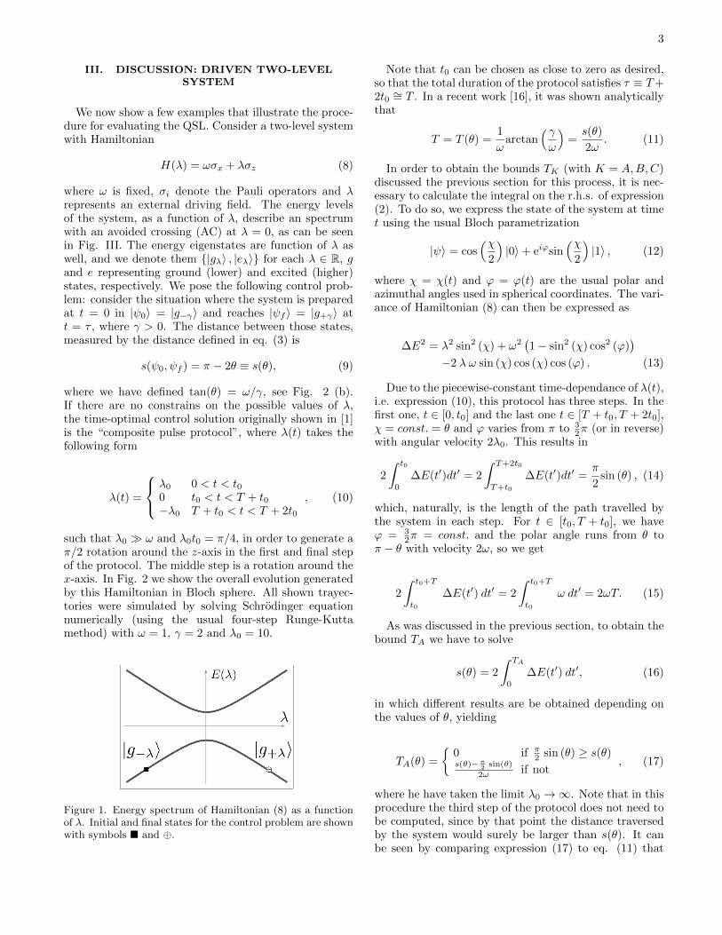
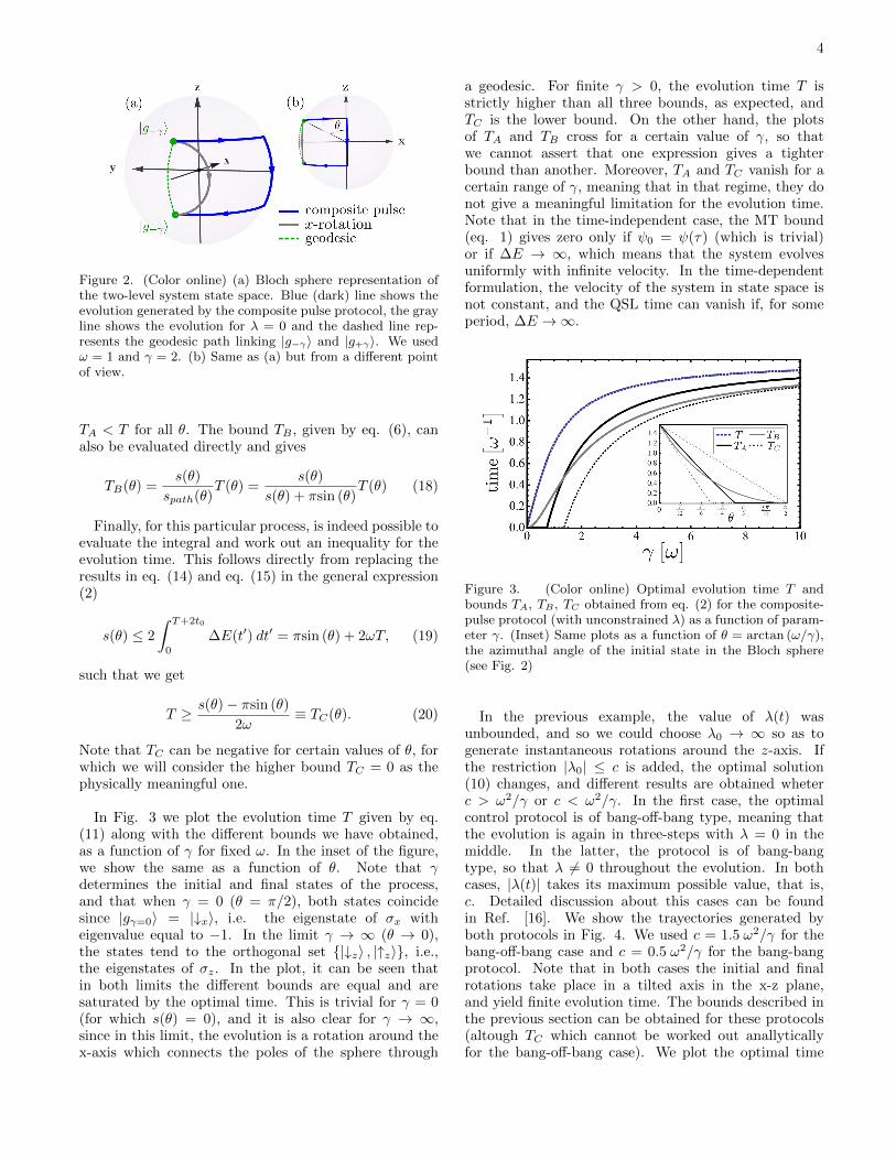
where ω is fixed, σi denote the Pauli operators and λrepresents an external driving field. The energy levelsof the system, as a function of λ, describe an spectrumwith an avoided crossing (AC) at λ = 0, as can be seenin Fig. III. The energy eigenstates are function of λ aswell, and we denote them {|gλ〉 , |eλ〉} for each λ ∈ R, gand e representing ground (lower) and excited (higher)states, respectively. We pose the following control prob-lem: consider the situation where the system is preparedat t = 0 in |ψ0〉 = |g−γ〉 and reaches |ψf 〉 = |g+γ〉 att = τ , where γ > 0. The distance between those states,measured by the distance defined in eq. (3) is

s(ψ0, ψf ) = π − 2θ ≡ s(θ), (9)

where we have defined tan(θ) = ω/γ, see Fig. 2 (b).If there are no constrains on the possible values of λ,the time-optimal control solution originally shown in [1]is the “composite pulse protocol”, where λ(t) takes thefollowing form

λ(t) =

λ0 0 < t < t00 t0 < t < T + t0−λ0 T + t0 < t < T + 2t0

, (10)

such that λ0 � ω and λ0t0 = π/4, in order to generate aπ/2 rotation around the z-axis in the first and final stepof the protocol. The middle step is a rotation around thex-axis. In Fig. 2 we show the overall evolution generatedby this Hamiltonian in Bloch sphere. All shown trayec-tories were simulated by solving Schrodinger equationnumerically (using the usual four-step Runge-Kuttamethod) with ω = 1, γ = 2 and λ0 = 10.

Figure 1. Energy spectrum of Hamiltonian (8) as a functionof λ. Initial and final states for the control problem are shownwith symbols � and ⊕.

Note that t0 can be chosen as close to zero as desired,so that the total duration of the protocol satisfies τ ≡ T+2t0 ∼= T . In a recent work [16], it was shown analyticallythat

T = T (θ) =1

ωarctan

( γω

)=s(θ)

2ω. (11)

In order to obtain the bounds TK (with K = A,B,C)discussed the previous section for this process, it is nec-essary to calculate the integral on the r.h.s. of expression(2). To do so, we express the state of the system at timet using the usual Bloch parametrization

|ψ〉 = cos(χ

2

)|0〉+ eiϕsin

(χ2

)|1〉 , (12)

where χ = χ(t) and ϕ = ϕ(t) are the usual polar andazimuthal angles used in spherical coordinates. The vari-ance of Hamiltonian (8) can then be expressed as

∆E2 = λ2 sin2 (χ) + ω2(1− sin2 (χ) cos2 (ϕ)

)−2 λ ω sin (χ) cos (χ) cos (ϕ) . (13)

Due to the piecewise-constant time-dependance of λ(t),i.e. expression (10), this protocol has three steps. In thefirst one, t ∈ [0, t0] and the last one t ∈ [T + t0, T + 2t0],χ = const. = θ and ϕ varies from π to 3

2π (or in reverse)with angular velocity 2λ0. This results in

2

∫ t0

0

∆E(t′)dt′ = 2

∫ T+2t0

T+t0

∆E(t′)dt′ =π

2sin (θ) , (14)

which, naturally, is the length of the path travelled bythe system in each step. For t ∈ [t0, T + t0], we haveϕ = 3

2π = const. and the polar angle runs from θ toπ − θ with velocity 2ω, so we get

2

∫ t0+T

t0

∆E(t′) dt′ = 2

∫ t0+T

t0

ω dt′ = 2ωT. (15)

As was discussed in the previous section, to obtain thebound TA we have to solve

s(θ) = 2

∫ TA

0

∆E(t′) dt′, (16)

in which different results are be obtained depending onthe values of θ, yielding

TA(θ) =

{0 if π

2 sin (θ) ≥ s(θ)s(θ)−π2 sin(θ)

2ω if not, (17)

where he have taken the limit λ0 →∞. Note that in thisprocedure the third step of the protocol does not need tobe computed, since by that point the distance traversedby the system would surely be larger than s(θ). It canbe seen by comparing expression (17) to eq. (11) that

4

Figure 2. (Color online) (a) Bloch sphere representation ofthe two-level system state space. Blue (dark) line shows theevolution generated by the composite pulse protocol, the grayline shows the evolution for λ = 0 and the dashed line rep-resents the geodesic path linking |g−γ〉 and |g+γ〉. We usedω = 1 and γ = 2. (b) Same as (a) but from a different pointof view.

TA < T for all θ. The bound TB , given by eq. (6), canalso be evaluated directly and gives

TB(θ) =s(θ)

spath(θ)T (θ) =

s(θ)

s(θ) + πsin (θ)T (θ) (18)

Finally, for this particular process, is indeed possible toevaluate the integral and work out an inequality for theevolution time. This follows directly from replacing theresults in eq. (14) and eq. (15) in the general expression(2)

s(θ) ≤ 2

∫ T+2t0

0

∆E(t′) dt′ = πsin (θ) + 2ωT, (19)

such that we get

T ≥ s(θ)− πsin (θ)

2ω≡ TC(θ). (20)

Note that TC can be negative for certain values of θ, forwhich we will consider the higher bound TC = 0 as thephysically meaningful one.

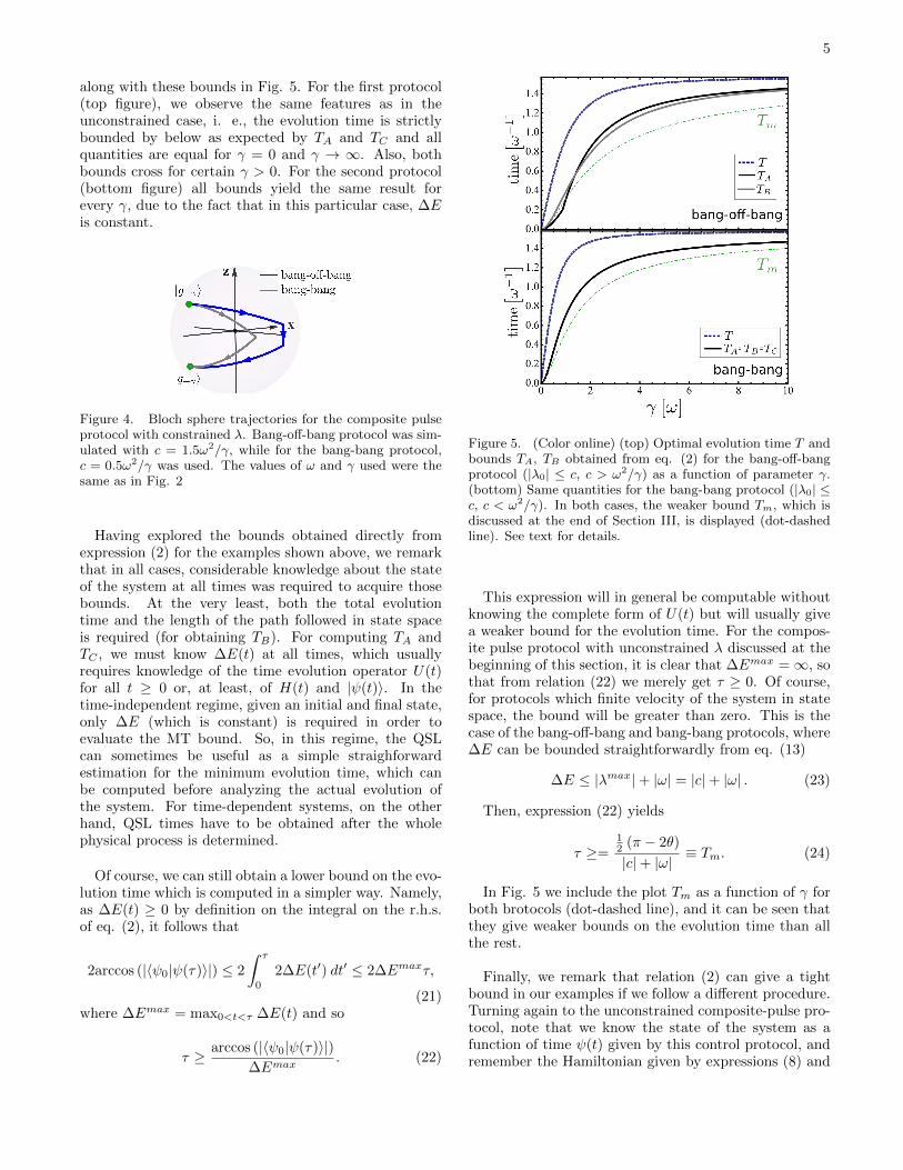
In Fig. 3 we plot the evolution time T given by eq.(11) along with the different bounds we have obtained,as a function of γ for fixed ω. In the inset of the figure,we show the same as a function of θ. Note that γdetermines the initial and final states of the process,and that when γ = 0 (θ = π/2), both states coincidesince |gγ=0〉 = |↓x〉, i.e. the eigenstate of σx witheigenvalue equal to −1. In the limit γ → ∞ (θ → 0),the states tend to the orthogonal set {|↓z〉 , |↑z〉}, i.e.,the eigenstates of σz. In the plot, it can be seen thatin both limits the different bounds are equal and aresaturated by the optimal time. This is trivial for γ = 0(for which s(θ) = 0), and it is also clear for γ → ∞,since in this limit, the evolution is a rotation around thex-axis which connects the poles of the sphere through

a geodesic. For finite γ > 0, the evolution time T isstrictly higher than all three bounds, as expected, andTC is the lower bound. On the other hand, the plotsof TA and TB cross for a certain value of γ, so thatwe cannot assert that one expression gives a tighterbound than another. Moreover, TA and TC vanish for acertain range of γ, meaning that in that regime, they donot give a meaningful limitation for the evolution time.Note that in the time-independent case, the MT bound(eq. 1) gives zero only if ψ0 = ψ(τ) (which is trivial)or if ∆E → ∞, which means that the system evolvesuniformly with infinite velocity. In the time-dependentformulation, the velocity of the system in state space isnot constant, and the QSL time can vanish if, for someperiod, ∆E →∞.

Figure 3. (Color online) Optimal evolution time T andbounds TA, TB , TC obtained from eq. (2) for the composite-pulse protocol (with unconstrained λ) as a function of param-eter γ. (Inset) Same plots as a function of θ = arctan (ω/γ),the azimuthal angle of the initial state in the Bloch sphere(see Fig. 2)

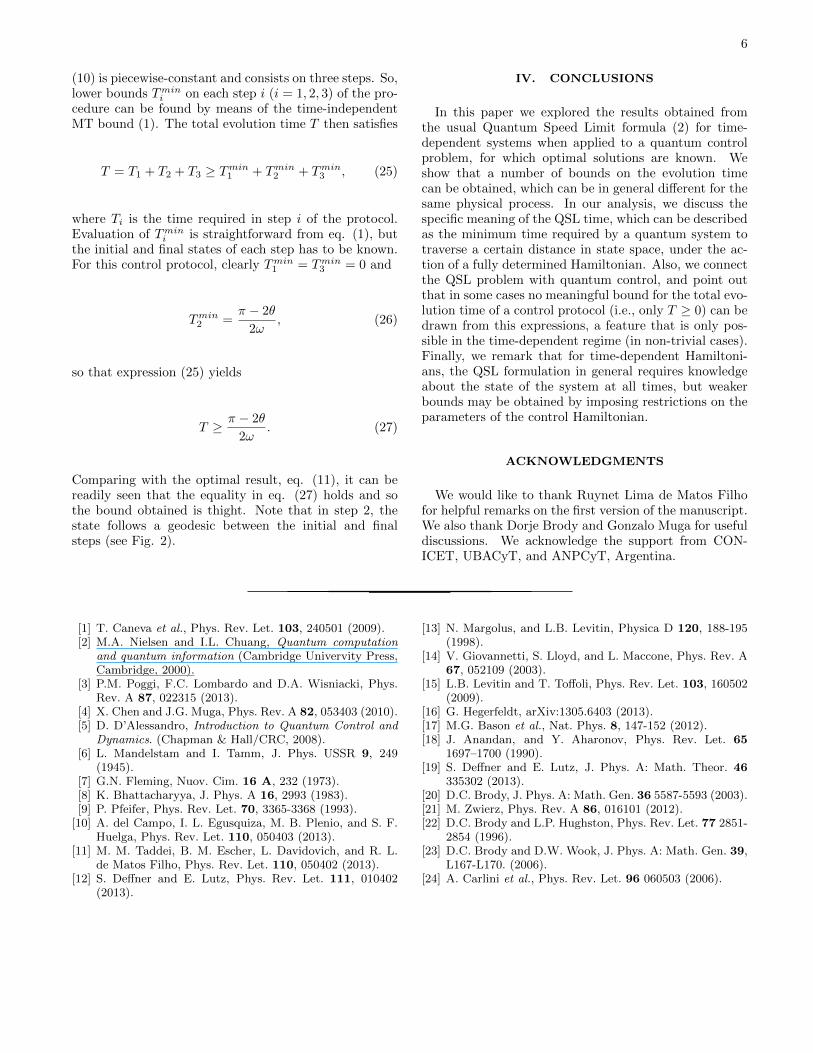
In the previous example, the value of λ(t) wasunbounded, and so we could choose λ0 → ∞ so as togenerate instantaneous rotations around the z-axis. Ifthe restriction |λ0| ≤ c is added, the optimal solution(10) changes, and different results are obtained wheterc > ω2/γ or c < ω2/γ. In the first case, the optimalcontrol protocol is of bang-off-bang type, meaning thatthe evolution is again in three-steps with λ = 0 in themiddle. In the latter, the protocol is of bang-bangtype, so that λ 6= 0 throughout the evolution. In bothcases, |λ(t)| takes its maximum possible value, that is,c. Detailed discussion about this cases can be foundin Ref. [16]. We show the trayectories generated byboth protocols in Fig. 4. We used c = 1.5 ω2/γ for thebang-off-bang case and c = 0.5 ω2/γ for the bang-bangprotocol. Note that in both cases the initial and finalrotations take place in a tilted axis in the x-z plane,and yield finite evolution time. The bounds described inthe previous section can be obtained for these protocols(altough TC which cannot be worked out anallyticallyfor the bang-off-bang case). We plot the optimal time

5

along with these bounds in Fig. 5. For the first protocol(top figure), we observe the same features as in theunconstrained case, i. e., the evolution time is strictlybounded by below as expected by TA and TC and allquantities are equal for γ = 0 and γ → ∞. Also, bothbounds cross for certain γ > 0. For the second protocol(bottom figure) all bounds yield the same result forevery γ, due to the fact that in this particular case, ∆Eis constant.

Figure 4. Bloch sphere trajectories for the composite pulseprotocol with constrained λ. Bang-off-bang protocol was sim-ulated with c = 1.5ω2/γ, while for the bang-bang protocol,c = 0.5ω2/γ was used. The values of ω and γ used were thesame as in Fig. 2

Having explored the bounds obtained directly fromexpression (2) for the examples shown above, we remarkthat in all cases, considerable knowledge about the stateof the system at all times was required to acquire thosebounds. At the very least, both the total evolutiontime and the length of the path followed in state spaceis required (for obtaining TB). For computing TA andTC , we must know ∆E(t) at all times, which usuallyrequires knowledge of the time evolution operator U(t)for all t ≥ 0 or, at least, of H(t) and |ψ(t)〉. In thetime-independent regime, given an initial and final state,only ∆E (which is constant) is required in order toevaluate the MT bound. So, in this regime, the QSLcan sometimes be useful as a simple straighforwardestimation for the minimum evolution time, which canbe computed before analyzing the actual evolution ofthe system. For time-dependent systems, on the otherhand, QSL times have to be obtained after the wholephysical process is determined.

Of course, we can still obtain a lower bound on the evo-lution time which is computed in a simpler way. Namely,as ∆E(t) ≥ 0 by definition on the integral on the r.h.s.of eq. (2), it follows that

2arccos (|〈ψ0|ψ(τ)〉|) ≤ 2

∫ τ

0

2∆E(t′) dt′ ≤ 2∆Emaxτ,

(21)where ∆Emax = max0<t<τ ∆E(t) and so

τ ≥ arccos (|〈ψ0|ψ(τ)〉|)∆Emax

. (22)

Figure 5. (Color online) (top) Optimal evolution time T andbounds TA, TB obtained from eq. (2) for the bang-off-bangprotocol (|λ0| ≤ c, c > ω2/γ) as a function of parameter γ.(bottom) Same quantities for the bang-bang protocol (|λ0| ≤c, c < ω2/γ). In both cases, the weaker bound Tm, which isdiscussed at the end of Section III, is displayed (dot-dashedline). See text for details.

This expression will in general be computable withoutknowing the complete form of U(t) but will usually givea weaker bound for the evolution time. For the compos-ite pulse protocol with unconstrained λ discussed at thebeginning of this section, it is clear that ∆Emax =∞, sothat from relation (22) we merely get τ ≥ 0. Of course,for protocols which finite velocity of the system in statespace, the bound will be greater than zero. This is thecase of the bang-off-bang and bang-bang protocols, where∆E can be bounded straightforwardly from eq. (13)

∆E ≤ |λmax|+ |ω| = |c|+ |ω| . (23)

Then, expression (22) yields

τ ≥=12 (π − 2θ)

|c|+ |ω|≡ Tm. (24)

In Fig. 5 we include the plot Tm as a function of γ forboth brotocols (dot-dashed line), and it can be seen thatthey give weaker bounds on the evolution time than allthe rest.

Finally, we remark that relation (2) can give a tightbound in our examples if we follow a different procedure.Turning again to the unconstrained composite-pulse pro-tocol, note that we know the state of the system as afunction of time ψ(t) given by this control protocol, andremember the Hamiltonian given by expressions (8) and

6

(10) is piecewise-constant and consists on three steps. So,lower bounds Tmini on each step i (i = 1, 2, 3) of the pro-cedure can be found by means of the time-independentMT bound (1). The total evolution time T then satisfies

T = T1 + T2 + T3 ≥ Tmin1 + Tmin2 + Tmin3 , (25)

where Ti is the time required in step i of the protocol.Evaluation of Tmini is straightforward from eq. (1), butthe initial and final states of each step has to be known.For this control protocol, clearly Tmin1 = Tmin3 = 0 and

Tmin2 =π − 2θ

2ω, (26)

so that expression (25) yields

T ≥ π − 2θ

2ω. (27)

Comparing with the optimal result, eq. (11), it can bereadily seen that the equality in eq. (27) holds and sothe bound obtained is thight. Note that in step 2, thestate follows a geodesic between the initial and finalsteps (see Fig. 2).

IV. CONCLUSIONS

In this paper we explored the results obtained fromthe usual Quantum Speed Limit formula (2) for time-dependent systems when applied to a quantum controlproblem, for which optimal solutions are known. Weshow that a number of bounds on the evolution timecan be obtained, which can be in general different for thesame physical process. In our analysis, we discuss thespecific meaning of the QSL time, which can be describedas the minimum time required by a quantum system totraverse a certain distance in state space, under the ac-tion of a fully determined Hamiltonian. Also, we connectthe QSL problem with quantum control, and point outthat in some cases no meaningful bound for the total evo-lution time of a control protocol (i.e., only T ≥ 0) can bedrawn from this expressions, a feature that is only pos-sible in the time-dependent regime (in non-trivial cases).Finally, we remark that for time-dependent Hamiltoni-ans, the QSL formulation in general requires knowledgeabout the state of the system at all times, but weakerbounds may be obtained by imposing restrictions on theparameters of the control Hamiltonian.

ACKNOWLEDGMENTS

We would like to thank Ruynet Lima de Matos Filhofor helpful remarks on the first version of the manuscript.We also thank Dorje Brody and Gonzalo Muga for usefuldiscussions. We acknowledge the support from CON-ICET, UBACyT, and ANPCyT, Argentina.

[1] T. Caneva et al., Phys. Rev. Let. 103, 240501 (2009).[2] M.A. Nielsen and I.L. Chuang, Quantum computation

and quantum information (Cambridge Univervity Press,Cambridge, 2000).

[3] P.M. Poggi, F.C. Lombardo and D.A. Wisniacki, Phys.Rev. A 87, 022315 (2013).

[4] X. Chen and J.G. Muga, Phys. Rev. A 82, 053403 (2010).[5] D. D’Alessandro, Introduction to Quantum Control and

Dynamics. (Chapman & Hall/CRC, 2008).[6] L. Mandelstam and I. Tamm, J. Phys. USSR 9, 249

(1945).[7] G.N. Fleming, Nuov. Cim. 16 A, 232 (1973).[8] K. Bhattacharyya, J. Phys. A 16, 2993 (1983).[9] P. Pfeifer, Phys. Rev. Let. 70, 3365-3368 (1993).

[10] A. del Campo, I. L. Egusquiza, M. B. Plenio, and S. F.Huelga, Phys. Rev. Let. 110, 050403 (2013).

[11] M. M. Taddei, B. M. Escher, L. Davidovich, and R. L.de Matos Filho, Phys. Rev. Let. 110, 050402 (2013).

[12] S. Deffner and E. Lutz, Phys. Rev. Let. 111, 010402(2013).

[13] N. Margolus, and L.B. Levitin, Physica D 120, 188-195(1998).

[14] V. Giovannetti, S. Lloyd, and L. Maccone, Phys. Rev. A67, 052109 (2003).

[15] L.B. Levitin and T. Toffoli, Phys. Rev. Let. 103, 160502(2009).

[16] G. Hegerfeldt, arXiv:1305.6403 (2013).[17] M.G. Bason et al., Nat. Phys. 8, 147-152 (2012).[18] J. Anandan, and Y. Aharonov, Phys. Rev. Let. 65

1697–1700 (1990).[19] S. Deffner and E. Lutz, J. Phys. A: Math. Theor. 46

335302 (2013).[20] D.C. Brody, J. Phys. A: Math. Gen. 36 5587-5593 (2003).[21] M. Zwierz, Phys. Rev. A 86, 016101 (2012).[22] D.C. Brody and L.P. Hughston, Phys. Rev. Let. 77 2851-

2854 (1996).[23] D.C. Brody and D.W. Wook, J. Phys. A: Math. Gen. 39,

L167-L170. (2006).[24] A. Carlini et al., Phys. Rev. Let. 96 060503 (2006).