Electronic copy available at: http://ssrn.com/abstract=1787625

The Predictive Power of Limit Order Book for Future Volatility, Trade

Price, and Speed of Trading

Pankaj Jain Associate Professor

The University of Memphis

Pawan Jain

Doctoral student The University of Memphis

Thomas H. McInish* Professor and Wunderlich Chair of Finance

The University of Memphis Voice: 901-277-9202 Fax: 901-678-3006

Email: tmcinish@memphis.edu

This Draft: 15 March, 2011

* Please address correspondence to: Professor Thomas H. McInish Department of Finance, Insurance, and Real Estate Fogelman College The University of Memphis Memphis, TN 38152

Electronic copy available at: http://ssrn.com/abstract=1787625

1

1 World Federation of Exchanges at www.world-exchanges.org.

The Predictive Power of Limit Order Book for Future Volatility, Trade Price, and Speed of Trading

Abstract

We investigate the information content of the limit order book (LOB) on the Tokyo Stock

Exchange, the world’s second largest order-driven exchange1. Microstructure parameters, such

as the current cost-to-trade 1% of average daily volume and order book slope, consistently and

significantly predict future price volatility, trade prices, and speed of trading. The shape of the

LOB on the bid side carries more predictive power than that on the ask side. Next, we document

that the average trade size is the driving force in the standard volume–volatility relationship.

Electronic copy available at: http://ssrn.com/abstract=1787625

The Predictive Power of Limit Order Book for Future Volatility, Trade

Price, and Speed of Trading

1. Introduction

The importance of electronic trading is growing and it is now the typical way of trading

equities. The heart of these modern trading systems is the limit order book (LOB), which

provides information about aggregate liquidity supply and trading interests (Naes & Skeljtorp,

2006). Beginning with the seminal work of Amihud and Mendelson (1986), many studies

document the role of liquidity as a determinant of expected returns (Brennan and Subrahmanyam

1996, Brennan, Chordia and Subrahmanyam 1998, Jacoby, Fowler and Gottesman 2000, Jones

2001 and Amihud, 2002). We investigate the relation between LOB liquidity and price volatility,

future trade prices, and speed of trading. Our findings are useful not only to understand the price

discovery process but also because volatility is a major determinant of options prices (Foucault ,

1999, Hasbrouck and Saar, 2002, Duong et al., 2008), and plays an important role in trade

execution strategies and investment decisions (Fleming et al., 2003).

Investigating the relation between the liquidity and future price volatility can also provide

insights about how information is incorporated into prices (Duong and Kalev, 2009). Placing a

limit buy (sell) order can be viewed as writing a free out-of-money put (call) option (Copeland

and Galai, 1983). The option-like characteristic of limit orders amplifies the influence of

volatility on its liquidity provision. Foucault, Moinas, and Theissen (2007) show that the

informed traders who expect high volatility, will post less aggressive limit orders, leading to a

thin book and large bid-ask spreads. Uninformed traders, who observe the large spread in the

1

book, will increase their expectation of future volatility and also be less willing to post limit

orders. As a result the overall liquidity provided by the LOB decreases when traders expect

higher future volatility. Furthermore, Foucault, Moinas, and Theissen (2007) also point out that a

thin LOB, as the result of high expected volatility, leads to future high realized volatility.

We study the informativeness of the order book on the world’s second largest fully

electronic order-driven exchange, the Tokyo Stock Exchange (TSE), where all of trading takes

place electronically without market markers. Orders are matched on price, then time priority, and

investors cannot choose their counterparties.

Our study contributes to the literature in the following ways. First, we characterize the

shape of the LOB by computing various composite measures of liquidity based on the first 5

steps of bid and ask prices and corresponding bid volume and ask volume. In addition to the

traditional liquidity measures such as spreads, we calculate new composite liquidity measures

that are more relevant in pure limit order book markets such as LOB slope, dispersion of limit

orders and cost to trade 1% of daily trading volume instantaneously by climbing up the book.

The main purpose of our paper is to conduct a horse race among these measures of liquidity to

test which one of them has the highest predictive power about future price volatility, future trade

prices, and speed of trading. As a by-product of our analyses, we contribute to the current debate

about the driving force behind the volume-volatility relationship. We also compare the predictive

power of buy and sell orders to test if buy orders have more information content for price

volatility than sell orders. Finally, we present a framework with which the basic principles of

demand and supply are incorporated in the price formation process.

We find that the cost to trade 1% of average daily volume is the dominant liquidity

measure that significantly and consistently predicts future price volatility, future trade prices and

2

speed of trading consistently across large, medium and small capitalization stocks. Order book

slope is also informative in explaining future price volatility and future trade prices for large cap

and mid cap stocks but is uninformative for small cap stocks.

To elaborate, the lower cost-to-trade on the bid (ask) side predicts that future trade price

will be higher (lower) than the previous trade price. Our interpretation of this finding is that the

higher liquidity on the bid (ask) side reflects an increased demand (supply) for the stock, which

in turn pushes the future trade prices higher (lower).

Lower cost-to-trade also predicts lower volatility of future return. Our interpretation of

this finding is that lower cost-to-trade reflects a highly liquid market that can easily

accommodate large buy or sell volumes, without affecting the prices significantly. There is an

outstanding debate in the literature whether average trade size or number of trades determine the

volume-volatility relationship. We find that the average trade size, and not the number of trades,

is the dominant determinant of the volume–volatility relationship. We also document that buy

orders are slightly more informative for predicting future return volatility than the sell orders.

Finally, trades occur more frequently when the cost to trade 1% of daily volume is lower.

Thus, lower cost-to-trade appears to attract more traders and high cost discourages frequent

trading. Traders like to wait for counter parties to arrive and fill the LOB to minimize their price

impact.

3

2. Literature Review

2.1. Liquidity and Future trade prices: Predictive power of the LOB

Although limit order book trading systems have been successful around the world, little

research has been done to address the value of the information contained in the order book. In

particular, one important question that remains unanswered is whether the demand and supply

schedules as expressed in the limit orders to buy and sell contain information about the future

trade prices.

In the traditional price discovery literature, it is a common belief that limit orders are not

as informative as market orders. Limit orders are generally viewed as non-aggressive orders that

supply liquidity to the market and market orders are viewed as aggressive orders that demand

liquidity. Glosten (1994), Rock (1996), and Seppi (1997) incorporated informed traders into their

models, assuming that they favor and actively submit market orders. This suggests that the order

book beyond the best bid and offer contains little, if any, information. Biais, Hillion, and Spatt

(1995), Grifiths et al. (2000), Hollifeld et al. (2003), and Ranaldo (2003) find that the rate of

limit order submissions increases with the size of the spread, and the depth at the top of both

sides of the book affects order choice.

Consistent with both Chakravarty and Holden (1995) and Wald and Horrigan (2005),

Kaniel and Liu (2006) provide a model based on Glosten and Milgrom (1985) that supports the

use of limit orders by informed traders. These authors emphasize the role of the informed

traders’ private information horizon as the key determinant of whether limit orders or market

orders are used. Market orders are used with short-lived information. When the expected time

4

horizon for their private information is longer, informed traders are more likely to submit limit

orders. Thus, when the probability that information is long-lived is sufficiently high, limit orders

might be more informative than market orders. Using an experimental design, Bloomfield,

O’Hara, and Saar (2005) found that in an electronic market, informed traders submit more limit

orders than market orders. Using SuperDot limit orders in the TORQ database, Harris and

Panchapagesan (2005) showed that the order book is informative, and that New York Stock

Exchange (NYSE) specialists use the book information in ways that favor them over the limit-

order traders.

This paper is part of an emerging literature about the informational content of the LOB.

We are particularly interested in the incremental informational content of the order book over

and above the best bid and offer quotes along with their respective depths

2.2. Liquidity-Volatility relation: Predictive power of the LOB

Foucault et al. (2007) develops a theoretical model for a limit order market where traders

differ in terms of their private information about future volatility. According to the model, the

LOB is a conduit for volatility information because of the option-like features of limit orders. As

prices of option depend on volatility, limit order traders should incorporate volatility information

in their limit order submissions. Therefore, the LOB should contain private volatility

information. In particular, Foucault et al. (2007) document that it is optimal for informed traders

with private information on volatility to bid less aggressively if volatility is expected to increase.

Empirical findings regarding the informativeness of the LOB for future volatility, are

presented in Ahn et al. (2001) and Pascual and Veredas (2006). Ahn et al. (2001) find a negative

relation between the market depth and future short term price volatility for the 33 component

5

stocks in the Hang Seng index of the Stock Exchange of Hong Kong. Pascual and Veredas

(2006) also provide supportive evidence for the informativeness of the LOB for the future

informational component of price volatility. Naes and Skjeltorp (2006) capture the LOB liquidity

by measuring the LOB slope and find a negative relationship between the liquidity and future

return volatility.

2.3. The volume– volatility relation: Trade size Vs. Number of trades

The volume–volatility relation is a well documented for most types of financial contracts,

including stocks, treasury bills, currencies and various futures contracts. But there is an ongoing

debate about the dominant factor behind this relationship. On the one hand, theoretical models

show that informed traders prefer to trade large amounts at any given price (Grundy and

McNichols, 1989; Holthausen and Verrecchia, 1990; Kim and Verrecchia, 1991). Trade size is

likely to be positively related to the quality of information possessed and will, therefore, be

positively correlated with price volatility (Chan and Fong, 2000). On the other hand, Kyle (1985)

and Admati and Pfleiderer (1988) indicate that a monopolist informed trader may camouflage his

trading activity by splitting one large trade into several small trades.

Jones et al. (1994) investigate, based on a sample of Nasdaq stocks, how daily price

volatility can be explained by daily number of trades and average trade size. They find that

number of trades virtually fully explains the volatility-volume relation, with average trade size

playing a trivial role. In a more recent study, Giot, et al. (2009) finds that the number of trades

remain the dominant factor behind the volume–volatility relation.

6

2.4. Informativeness of buy orders versus sell orders

Burdett and O'Hara (1987) observe that large buyers are more likely to be motivated by

information than are large sellers. Similarly, Griffiths et al. (2000) also provide evidence that

aggressive buy orders on the Toronto Stock Exchange are more informative than aggressive sell

orders. Based on these findings, we argue that the information advantage of buyers over sellers

are not limited only to market orders, but also extends to limit orders, which are less aggressive.

Therefore, we hypothesize that the limit orders on the bid side are more informative than the

limit orders on the ask side.

2.4. Liquidity and Speed of Trading

Boehmer (2005) analyzes market orders on Nasdaq and at the NYSE’s auction market.

He finds an inverse relationship between execution speed and trading costs as measured by the

effective spread. Ellul, Holdings, Jain and Jennings (2007) provide support for this finding. But,

the relationship might change when we consider liquidity beyond the best quotes. If the LOB is

thick, then the cost of walking down/up the LOB is lower as compared to when the LOB is thin.

7

3. The data

Our sample includes one year of order book data for all companies listed on the first

section of the Tokyo stock exchange (TSE). The TSE, with a total market cap of about $3

trillion, is the second largest stock exchange in the world, the largest being the NYSE Euronext

(TSE annual report, 2009). The data comprise every order and trade on the TSE. The dataset also

provides the five best bid and ask quotes, and the associated depth. The period of our analysis

begins from July 1, 2007 and ends on June 30, 2008. We obtain these data from the Nikkei

Digital Media Inc. (NEEDS) database. TSE trading takes place in two different trading sessions.

The morning session begins at 9:00 a.m. and ends at 11:00 a.m., while the afternoon session

begins at 12:30 p.m. and ends at 3 p.m. The dataset also includes data from the pre-trading and

post-trading periods; those observations are removed for the final sample. Various filters are

used to eliminate data errors. We use these data to ascertain the most recently disseminated

quotes and quote sizes on both sides of the market.

For this study, we limit our attention to the stocks included in the Tokyo Stock Price

Index (TOPIX), which is a composite index of all the domestic common stocks listed on the

exchange. The TOPIX, is considered the best indicator of the financial condition of the Japanese

stock market (TSE annual report, 2009). The TOPIX is a free-float adjusted market

capitalization-weighted index that is calculated based on all the domestic common stocks listed

on the TSE First Section. TOPIX shows the measure of current market capitalization assuming

that market capitalization as of the base date (January 4, 1968) is 100 points. Size-based Sub-

Indices consist of three indices created by dividing the component stock of the TOPIX into three

categories based on market capitalization and liquidity. The largest 100 stocks and the next

8

largest 400 stocks are in the TOPIX 100 Large-Sized Stocks Index and the TOPIX Mid400

Medium-Sized Stocks Index, respectively. The remaining stocks of the TSE first section are in

the TOPIX Small-Sized Stocks Index.

4. Measures of liquidity

Liquidity is difficult to define and even more difficult to estimate. Kyle (1985) notes that

‘‘liquidity is a slippery and elusive concept, in part because it encompasses a number of

transactional properties of markets, these include tightness, depth, and resiliency,’’ (p. 1316).

Empirical liquidity definitions span direct trading costs (tightness), measured by the bid–ask

spread (quoted or effective), to indirect trading costs (depth and resiliency), measured by price

impact. The literature provides a menu of measures and proxies to consider for estimating

liquidity.

4.1. Spread

The first class of liquidity estimators measure trading costs directly. Proportional bid-ask

spread is commonly measured as the difference between the best ask quote and best bid quote as

a percentage of bid-ask midpoint. Bollerslev and Melvin (1994) construct a microstructure model

that shows how price volatility and bid-ask spreads are linked. Expected volatility increase goes

hand in hand with an increase in the bid-ask spread (Booth and Gurun, 2008). Empirical studies

supporting this positive relationship include Hasbrouck (1999), Bollerslev and Melvin (1994)

and Kalimipalli and Warga (2002), who show that this phenomenon exists in common stocks,

9

foreign exchange rates and corporate bonds, respectively. Rahman et al. (2002) use a

GARCH(1,1) model and find that all but eight of the thirty NASDAQ stocks exhibit a positive

relationship between lagged bid-ask spread and return volatility. The significance of the positive

results indicates that “…information arrival would be expected to induce an increase in future

volatility and this would in turn have the effect of widening the contemporaneous bid-ask

spread” (Rahman et al. 2002). Recently, Higgs and Worthington (2008) document a significantly

negative relationship between the bid-ask spread and return volatility.

4.2. Order book slope

Goldstein and Kavajecz (2004) provide evidence of a negative relation between the shape

of the order book and future price volatility during an extreme market movement. More recently,

Naes and Skjeltorp (2006) and Duang and Kalev (2009) document a negative relationship

between the price volatility and order book slope in the Norwegian and Australian markets,

respectively. In this paper, we test whether the order book slope provides the information about

the future price volatility in the Japanese market.

A significant negative relationship is found between the order book slope and the

coefficient of variation in analysts’ earnings forecasts, i.e., the greater the disagreement among

analysts, the more gentle the average slope of the order book (Naes and Skjeltorp, 2006). This

result suggests that the order book slope proxies for dispersed beliefs about asset values. Applied

to the two securities in Figure 1, this would imply that investors disagree more about the value of

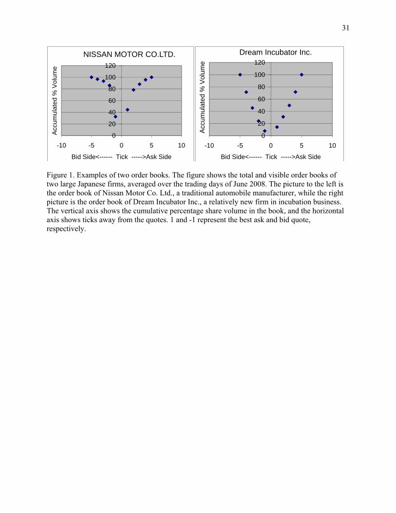
Dream Incubator Inc than Nissan Motor Co. Ltd. Looking at the main characteristics of the two

firms, this makes sense. Nissan Motor Co. Ltd. is a leading automobile manufacturer, with over

10

50,000 employees in over 50 countries worldwide, with well known operations, a long history,

and a large amount of available information, including experts’ analysis. Dream Incubator Inc,

on the other hand, is a relatively young incubator firm with fewer than 100 employees and very

uncertain future income prospects.

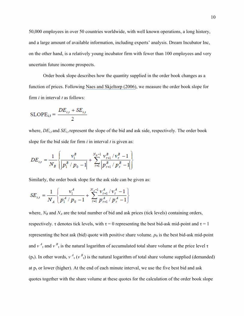
Order book slope describes how the quantity supplied in the order book changes as a

function of prices. Following Naes and Skjeltorp (2006), we measure the order book slope for

firm i in interval t as follows:

where, DEi,t and SEi,t represent the slope of the bid and ask side, respectively. The order book

slope for the bid side for firm i in interval t is given as:

Similarly, the order book slope for the ask side can be given as:

where, NB and NA are the total number of bid and ask prices (tick levels) containing orders,

respectively. τ denotes tick levels, with τ = 0 representing the best bid-ask mid-point and τ = 1

representing the best ask (bid) quote with positive share volume. p0 is the best bid-ask mid-point

and v Aτ and v Bτ is the natural logarithm of accumulated total share volume at the price level τ

(pτ). In other words, v Aτ (v Bτ) is the natural logarithm of total share volume supplied (demanded)

at pτ or lower (higher). At the end of each minute interval, we use the five best bid and ask

quotes together with the share volume at these quotes for the calculation of the order book slope

11

for that particular interval. We divide the slope measure by 100 to scale the parameter estimates

in the regressions in the next sections.

4.3. Other measures of liquidity

In addition to the above two well established liquidity measures, we also investigate

several newer measures of liquidity that are more relevant in the context of a pure limit order

book.

4.3.1. Order book dispersion

Foucault, Kaden & Kandel (2005) find that the proportion of patient traders in the

population and the order arrival rate are the key determinants of the limit order book dynamics.

Traders submit aggressive limit orders (improve upon quoted spreads by large amounts) when

the proportion of patient traders is large or when the order arrival rate is low. The order book

dispersion measure is designed to capture this idea. This measure shows how clustered or

dispersed limit orders are in the LOB. It measures how tightly the orders are placed to each other

or how closely they are to the mid-quote. The higher the dispersion, the less tight the book is,

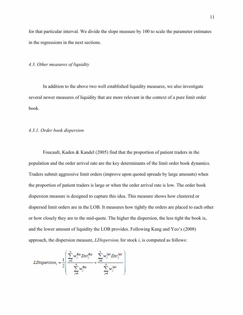
and the lower amount of liquidity the LOB provides. Following Kang and Yeo’s (2008)

approach, the dispersion measure, LDispersioni for stock i, is computed as follows:

12

Dstj is the price interval between the jth best bid or offer and its next better quote. Hence,

DstjBuy= (Bidj-Bidj-1) and Dstj

sell= (Askj-Askj-1). We weight Dstj by the size of limit orders: the

weight, wj, is the size of the corresponding bid or offer limit order. The weight is normalized by

dividing each weight by the sum of all the weights. The LDispersion measure shows the

competitiveness between the limit order traders. Under fierce competition, the limit order traders

undercut each other to gain price priority, and the LDispersion measure tends to be small (Kang

and Yeo, 2008).

4.3.2. The Cost-to-trade: an enhanced depth measure

Another measure of the liquidity provided in the LOB is based on how well high volume

orders are handled. A deep LOB can absorb a sudden surge in the demand of liquidity with

minimal price impact. Market buy (sell) orders are first executed against the limit sell (buy)

orders at the best ask (bid) and subsequently walk down (climb up) the book for execution of the

remaining volume at worse prices. Similarly, when multiple orders arrive successively, the

orders arriving later may have to walk down or climb up the book. Imagine there is a marketable

limit order of sufficient size to entirely deplete the depth at the best price. A second marketable

limit order appearing before the book is replenished will execute against the remaining best

quotes. The further that marketable limit orders walk up or down the book, the larger the

difference between the execution price and the mid-quote is, and, therefore, the more costly the

trading process will be for the marketable limit order traders (Benston, Irvine and Kandel, 2002).

To calculate our measure, we follow Kang and Yeo approach (2008). For each stock, we

estimate the impact of a sudden surge in the demand for liquidity separately on the buy and the

13

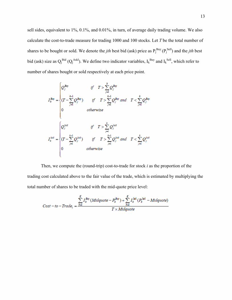
sell sides, equivalent to 1%, 0.1%, and 0.01%, in turn, of average daily trading volume. We also

calculate the cost-to-trade measure for trading 1000 and 100 stocks. Let T be the total number of

shares to be bought or sold. We denote the jth best bid (ask) price as PjBuy (Pj

Sell) and the jth best

bid (ask) size as QjBid (Qj

Askl). We define two indicator variables, IkBuy and Ik

Sell, which refer to

number of shares bought or sold respectively at each price point.

Then, we compute the (round-trip) cost-to-trade for stock i as the proportion of the

trading cost calculated above to the fair value of the trade, which is estimated by multiplying the

total number of shares to be traded with the mid-quote price level:

14

5. Results

5.1. Descriptive statistics

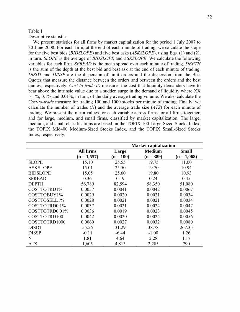
Table 1 provides summary statistics for our sample of 1,557 stocks. We average the

liquidity measures across one minute intervals for each stock and then report the measures

averaged across stocks. We present the results for the whole sample and also for large-, mid- and

small-cap stocks separately. The mean order book slope of 25.55 for large-cap stocks is more

than two times the mean of 11.00 for small-cap stocks. Thus, the typical order book slope is

steeper for large-cap stocks than for mid- and small-cap stocks. The order book on the buy side is

steeper than on the sell side. The steeper the order book slope, the higher the liquidity.

For the LOB dispersion measures based on the best five quotes, the mean of DISDT is

55.56 JPY. This measure decreases as size increases, indicating that large stocks are more liquid.

As for the cost-to-trade, it costs market-order traders 0.57% more to buy and sell 1% of the

stock’s average daily trading volume than it costs limit order traders. The cost to trade is higher

for small-cap stocks. This measure also decreases if the trader buys a lower proportion of stocks.

Hence, we see a lower cost for trading 0.1% and 0.01% of average daily trading volume. Large-

caps stocks trade 4.6 times each minute while mid-cap stocks trade 2.28 times each minute and

small-cap stocks trade 1.17 times each minute. A similar pattern appears for average trade size.

The bid-ask spread is also lower for large-cap stocks and increases as the size decreases, while,

the depth at the best quote is highest for large-cap stocks.

15

5.2. Predicting the future trade price movement

We test the predictive power of various LOB liquidity measures for predicting the future

trade price movements. For each firm in our sample, we estimate the following regression model:

PRIi,t = αi + αib BIDLIQUIDITYit-j + αia ASKLIQUIDITYit-j + µi,t

where PRIi,t is the magnitude of the trade price change. We calculate the Elasticity based

liquidity measures, slope for the five best bids (BIDSLOPE) and five best asks (ASKSLOPE) for

each firm, for every change in LOB. We also calculate cost based liquidity measures. The cost

that liquidity demanders bear to buy 1% of the daily average trading volume, CTSELLi,t-1, is the

cost that liquidity demanders bear to sell 1% of the daily average trading volume. is the change

operator. α are parameters to be estimated, and µi,t is a random error term. The subscripts i and t

indicate firm i and period t, respectively.

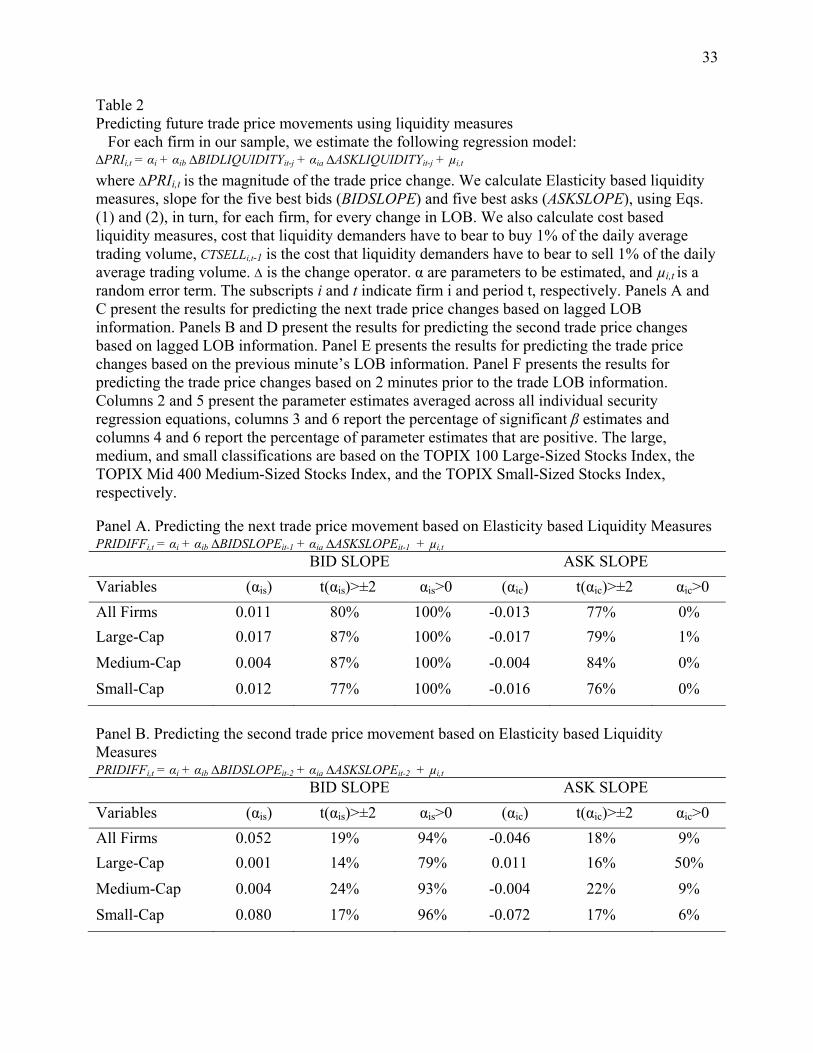
Results are summarized in Table 2. Examining Panels A and C, we find a significant

relation between bid- and ask-side liquidity and future price movements for both elasticity based

and cost based liquidity measures for 77% to 80% of our sample firms. As the bid (ask) side

liquidity increases, the next trade prices goes up (down). This result is intuitive and can be

explained by the basic principles of demand and supply. As the bid (ask) side liquidity increases,

demand (supply) for that security increases and hence, the price goes up (down). This result

might prove useful for high frequency algorithmic traders.

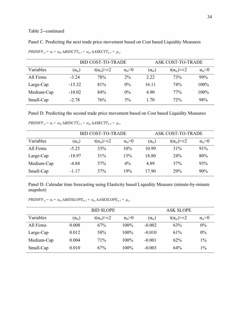
However, when we try to predict the second trade based on prior LOB information, the

predictive power of different liquidity measures drops significantly. When we compare the

results in Table 2, Panels B and D, we see that cost based liquidity measures are better predictors

than elasticity based measures.

16

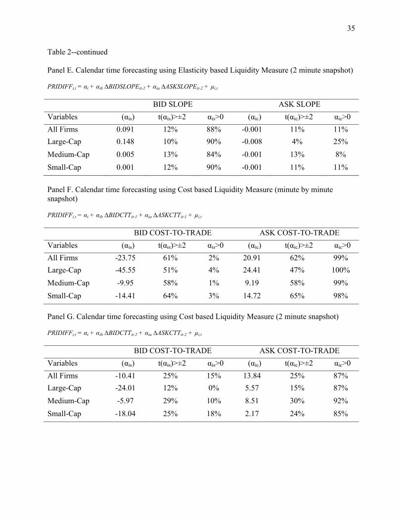
Table 2, Panel E, presents the results for predicting trade price changes based on the

previous minute’s LOB information. The prior minute’s LOB information significantly predicts

future trade price movements for about 62% of firms. The minute-by-minute results are weaker

than the trade-by-trade results, but the former may still be useful in formulating trading

strategies. Table 2, Panel F, presents the results for predicting trade price changes based on 2

minutes prior to the trade LOB information. LOB liquidity has very low predictive power

beyond the 1 minute time interval.

5.3. Volatility and bid-ask spread

Supporters of the specialist system often argue that immediacy of execution is critical for

a well-functioning capital market and that a designated market maker is necessary for

guaranteeing continuous immediacy at a reasonable cost. One of the most frequently examined

measures of liquidity is the quoted bid-ask spread, since the difference between the quotes

represents the round trip cost of immediately reversing a trade position. But on the TSE there are

no designated market maker. Hence, it is of particular interest to understand the variation in bid-

ask spread in the completely order-driven Japanese market.

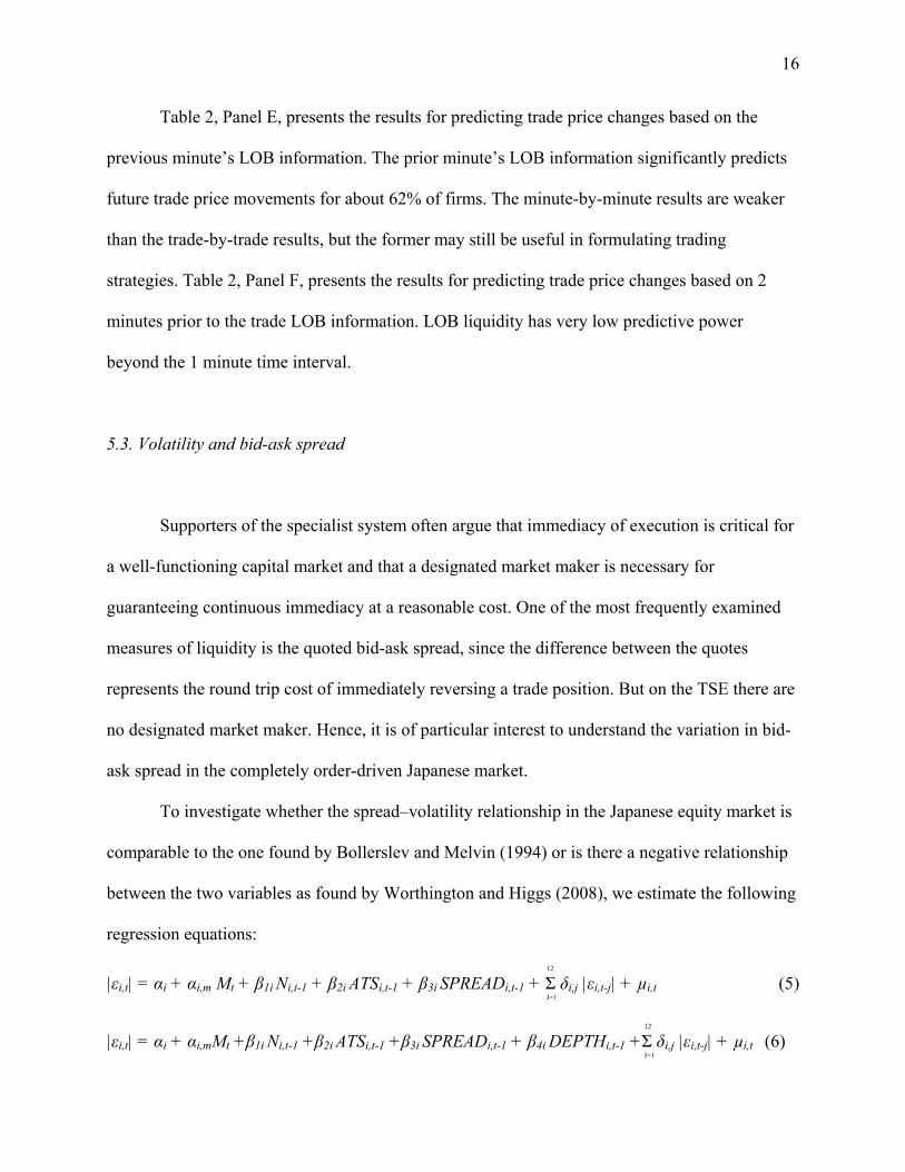
To investigate whether the spread–volatility relationship in the Japanese equity market is

comparable to the one found by Bollerslev and Melvin (1994) or is there a negative relationship

between the two variables as found by Worthington and Higgs (2008), we estimate the following

regression equations:

12

|εi,t| = αi + αi,m Mt + β1i Ni,t-1 + β2i ATSi,t-1 + β3i SPREADi,t-1 + Σ δi,j |εi,t-j| + µi,t (5) J=1

12

|εi,t| = αi + αi,mMt +β1i Ni,t-1 +β2i ATSi,t-1 +β3i SPREADi,t-1 + β4i DEPTHi,t-1 +Σ δi,j |εi,t-j| + µi,t (6) J=1

17

where, |εi,t| is the absolute value of the return on security i in period t, conditional on its own 12

lags and day-of-week dummies, Mt is a dummy variable that is equal to 1 for Mondays and 0

otherwise, ATSi,t-1 is the average trade size, Ni,t-1 is the number of transactions for security i on

period t, and the coefficients δi,j measure the persistence in volatility. The regressions are

estimated for each security and then the parameter estimates are averaged across securities.

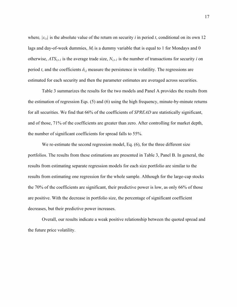
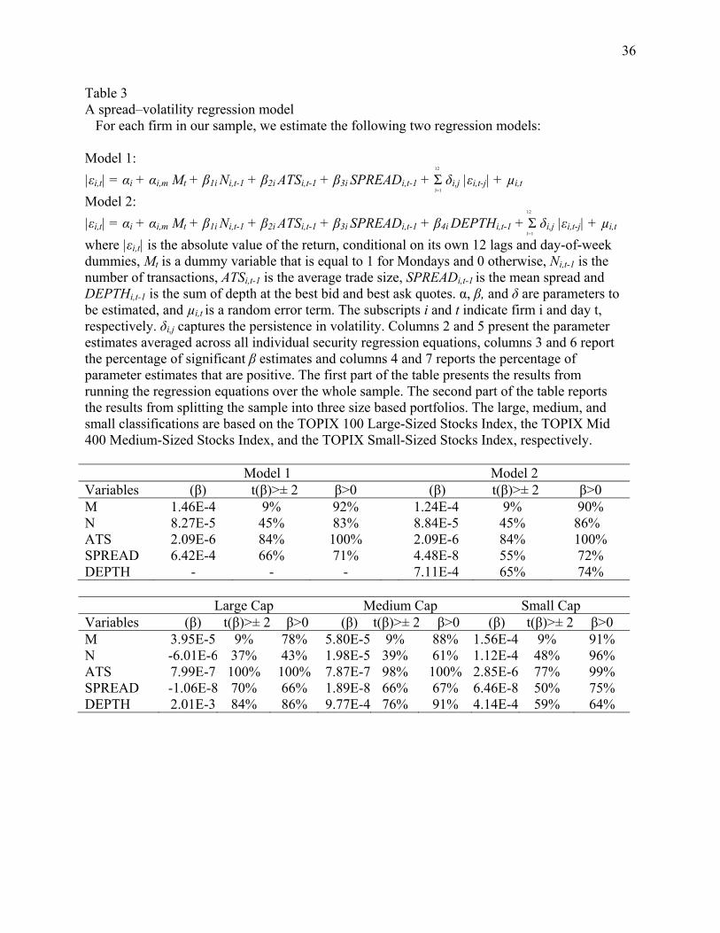
Table 3 summarizes the results for the two models and Panel A provides the results from

the estimation of regression Eqs. (5) and (6) using the high frequency, minute-by-minute returns

for all securities. We find that 66% of the coefficients of SPREAD are statistically significant,

and of those, 71% of the coefficients are greater than zero. After controlling for market depth,

the number of significant coefficients for spread falls to 55%.

We re-estimate the second regression model, Eq. (6), for the three different size

portfolios. The results from these estimations are presented in Table 3, Panel B. In general, the

results from estimating separate regression models for each size portfolio are similar to the

results from estimating one regression for the whole sample. Although for the large-cap stocks

the 70% of the coefficients are significant, their predictive power is low, as only 66% of those

are positive. With the decrease in portfolio size, the percentage of significant coefficient

decreases, but their predictive power increases.

Overall, our results indicate a weak positive relationship between the quoted spread and

the future price volatility.

18

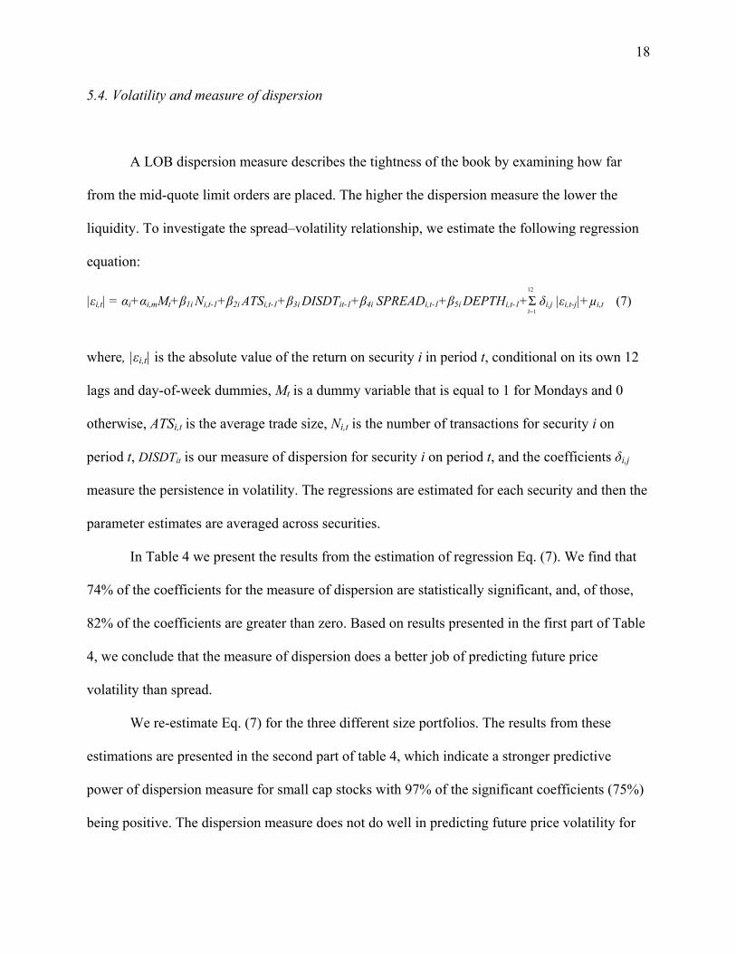
5.4. Volatility and measure of dispersion

A LOB dispersion measure describes the tightness of the book by examining how far

from the mid-quote limit orders are placed. The higher the dispersion measure the lower the

liquidity. To investigate the spread–volatility relationship, we estimate the following regression

equation:

12

|εi,t| = αi+αi,mMt+β1i Ni,t-1+β2i ATSi,t-1+β3i DISDTit-1+β4i SPREADi,t-1+β5i DEPTHi,t-1+Σ δi,j |εi,t-j|+µi,t (7) J=1

where, |εi,t| is the absolute value of the return on security i in period t, conditional on its own 12

lags and day-of-week dummies, Mt is a dummy variable that is equal to 1 for Mondays and 0

otherwise, ATSi,t is the average trade size, Ni,t is the number of transactions for security i on

period t, DISDTit is our measure of dispersion for security i on period t, and the coefficients δi,j

measure the persistence in volatility. The regressions are estimated for each security and then the

parameter estimates are averaged across securities.

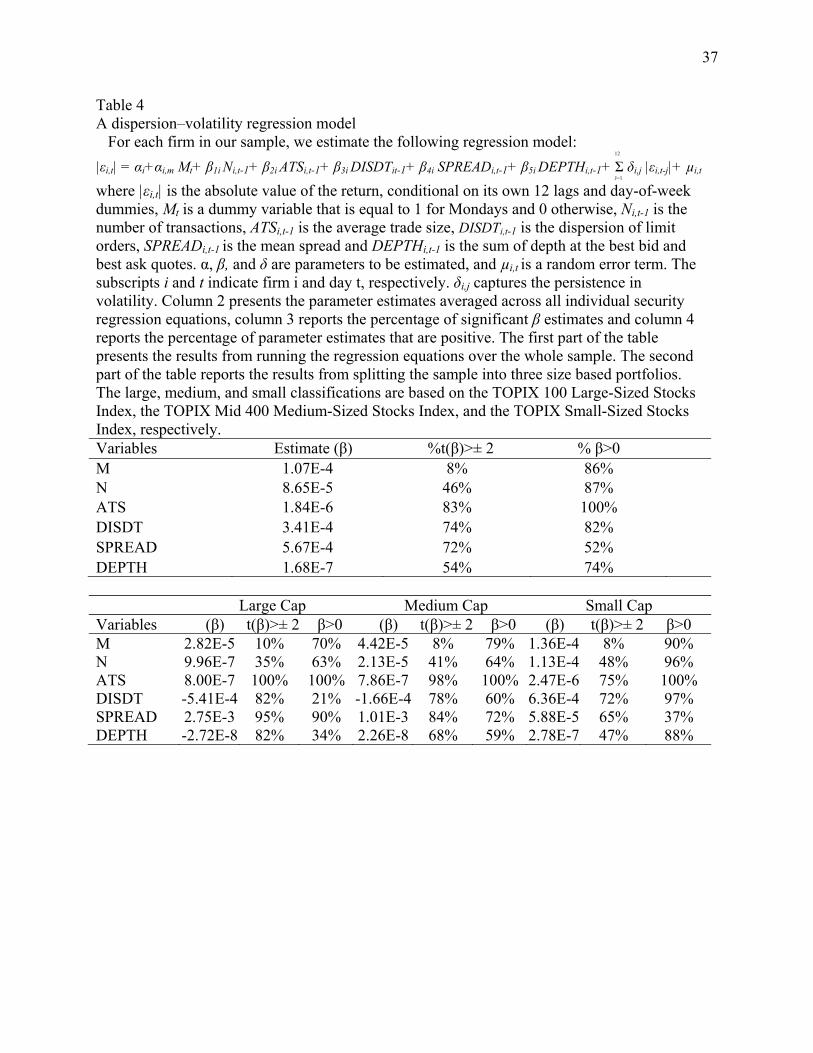
In Table 4 we present the results from the estimation of regression Eq. (7). We find that

74% of the coefficients for the measure of dispersion are statistically significant, and, of those,

82% of the coefficients are greater than zero. Based on results presented in the first part of Table

4, we conclude that the measure of dispersion does a better job of predicting future price

volatility than spread.

We re-estimate Eq. (7) for the three different size portfolios. The results from these

estimations are presented in the second part of table 4, which indicate a stronger predictive

power of dispersion measure for small cap stocks with 97% of the significant coefficients (75%)

being positive. The dispersion measure does not do well in predicting future price volatility for

19

large cap and mid cap stocks and for the large cap firms, we get counter-intuitive results with

majority (79%) of significant coefficients being negative.

5.5. Volatility and order book slope

To examine the informativeness of the order book slope, we estimate the following

regression model:

12

|εi,t| = αi+αi,mMt+β1i Ni,t-1+β2i ATSi,t-1+β3i SLOPEit-1+β4i SPREADi,t-1+β5i DEPTHi,t-1+Σ δi,j|εi,t-j|+µi,t (8) J=1

where, |εi,t| is the absolute value of the return on security i in period t, conditional on its own 12

lags and day-of-week dummies, Mt is a dummy variable that is equal to 1 for Mondays and 0

otherwise, ATSi,t-1 is the average trade size, Ni,t-1 is the number of transactions for security i on

period t, SLOPEit-1 is our measure of order book slope for security i on period t-1, and the

coefficients δi,j measure the persistence in volatility. The regressions are estimated for each

security and then the parameter estimates are averaged across securities.

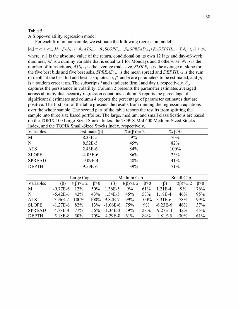
Results of the estimation of Eq. 8 are presented in Table 5. First, note that the coefficients

on the order book slope variable (SLOPE) are negative and significant for 86% of the stocks.

The gentler the slope, the higher the future volatility. Again, average trade size significantly

predicts future price volatility.

To further analyze the relationship between LOB slope and future price volatility, we re-

estimate Eq. (8) for portfolios of three different sizes and presented the results in Table 5. These

results indicate strong predictive power of order book slope for large- and mid-cap stocks. About

95% (86%) of the estimates for the slope coefficients for large cap (medium cap) are significant

at 5 % level and of those, about 87% (91%) are negatively significant. While only 63% of the

20

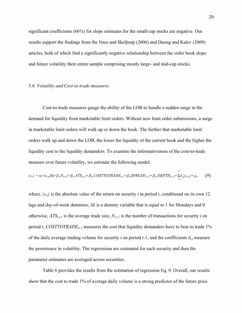
significant coefficients (66%) for slope estimates for the small-cap stocks are negative. Our

results support the findings from the Naes and Skeljtorp (2006) and Duong and Kalev (2009)

articles, both of which find a significantly negative relationship between the order book slope

and future volatility their entire sample comprising mostly large- and mid-cap stocks.

5.6. Volatility and Cost-to-trade measures

Cost-to-trade measures gauge the ability of the LOB to handle a sudden surge in the

demand for liquidity from marketable limit orders. Without new limit order submissions, a surge

in marketable limit orders will walk up or down the book. The further that marketable limit

orders walk up and down the LOB, the lower the liquidity of the current book and the higher the

liquidity cost to the liquidity demanders. To examine the informativeness of the cost-to-trade

measure over future volatility, we estimate the following model:

12

|εi,t| = αi+αi,mMt+β1iNi,t-1+β2i ATSi,t-1+β3i COSTTOTRADEit-1+β4iSPREADi,t-1+β5i DEPTHi,t-1+Σδi,j|εi,t-j|+µi,t (9) J=1

where, |εi,t| is the absolute value of the return on security i in period t, conditional on its own 12

lags and day-of-week dummies, Mt is a dummy variable that is equal to 1 for Mondays and 0

otherwise, ATSi,t-1 is the average trade size, Ni,t-1 is the number of transactions for security i on

period t, COSTTOTRADEit-1 measures the cost that liquidity demanders have to bear to trade 1%

of the daily average trading volume for security i on period t-1, and the coefficients δi,j measure

the persistence in volatility. The regressions are estimated for each security and then the

parameter estimates are averaged across securities.

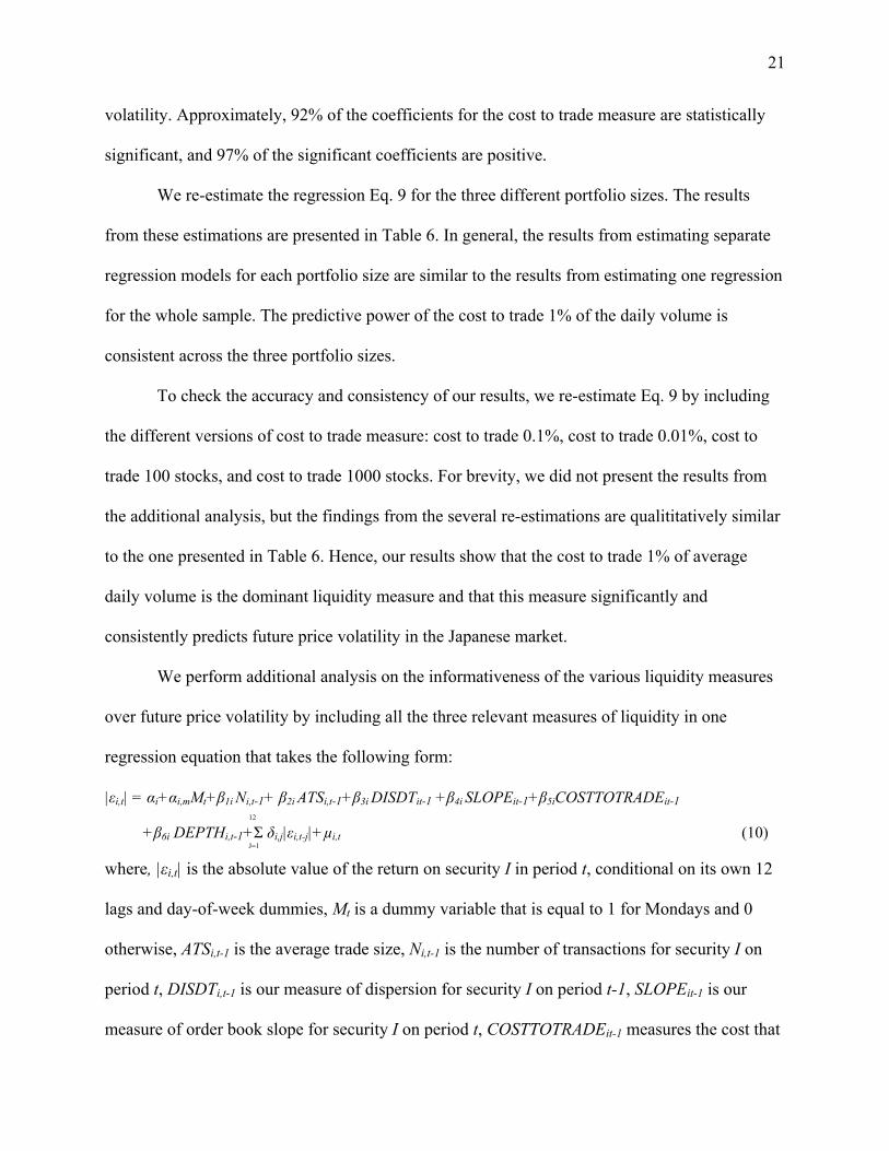
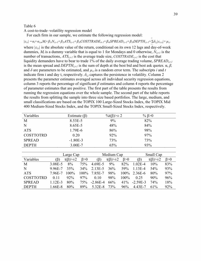
Table 6 provides the results from the estimation of regression Eq. 9. Overall, our results

show that the cost to trade 1% of average daily volume is a strong predictor of the future price

21

volatility. Approximately, 92% of the coefficients for the cost to trade measure are statistically

significant, and 97% of the significant coefficients are positive.

We re-estimate the regression Eq. 9 for the three different portfolio sizes. The results

from these estimations are presented in Table 6. In general, the results from estimating separate

regression models for each portfolio size are similar to the results from estimating one regression

for the whole sample. The predictive power of the cost to trade 1% of the daily volume is

consistent across the three portfolio sizes.

To check the accuracy and consistency of our results, we re-estimate Eq. 9 by including

the different versions of cost to trade measure: cost to trade 0.1%, cost to trade 0.01%, cost to

trade 100 stocks, and cost to trade 1000 stocks. For brevity, we did not present the results from

the additional analysis, but the findings from the several re-estimations are qualititatively similar

to the one presented in Table 6. Hence, our results show that the cost to trade 1% of average

daily volume is the dominant liquidity measure and that this measure significantly and

consistently predicts future price volatility in the Japanese market.

We perform additional analysis on the informativeness of the various liquidity measures

over future price volatility by including all the three relevant measures of liquidity in one

regression equation that takes the following form:

|εi,t| = αi+αi,mMt+β1i Ni,t-1+ β2i ATSi,t-1+β3i DISDTit-1 +β4i SLOPEit-1+β5iCOSTTOTRADEit-1 12

+β6i DEPTHi,t-1+Σ δi,j|εi,t-j|+µi,t (10) J=1

where, |εi,t| is the absolute value of the return on security I in period t, conditional on its own 12

lags and day-of-week dummies, Mt is a dummy variable that is equal to 1 for Mondays and 0

otherwise, ATSi,t-1 is the average trade size, Ni,t-1 is the number of transactions for security I on

period t, DISDTi,t-1 is our measure of dispersion for security I on period t-1, SLOPEit-1 is our

measure of order book slope for security I on period t, COSTTOTRADEit-1 measures the cost that

22

liquidity demanders have to bear to trade 1% of the daily average trading volume for security I

on period t-1, and the coefficients δi,j measure the persistence in volatility. The regressions are

estimated for each security and then the parameter estimates are averaged across securities.

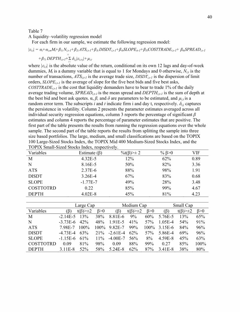
The results are summarized in Table 7. Consistent with the results obtained in Table 6,

the results of Table 7 indicate that the cost to trade measure is more informative, than the other

two liquidity measures, over future price volatility. The cost to trade 1% of average daily volume

is informative over future price volatility in 85% of stocks and is consistent across the different

size portfolios. In contrast, the predictive power of the measure of dispersion (LOB slope) is

evident in only 67% (49%) of the sample stocks. Also, neither of the two measures is consistent

across the different firm size portfolios. In general, measure of dispersion are better predictors

for small-cap stocks and LOB slope is superior for predicting future price volatility for large- and

mid-cap firms.

5.7. The volume– volatility relation in an order-driven market

In this section we investigate whether the volume–volatility relationship in the Japanese

equity market is comparable to the one found in the US market by Jones et al., (1994), in the UK

market by Huang and Masulis (2003), and in Norway\ by Naes and Skeljtorp (2006). We follow

the approachs pf Jones et al. (1994) and Naes and Skeljtorp (2006).

First, we measure daily return volatility by estimating the following regression for each

security i

23

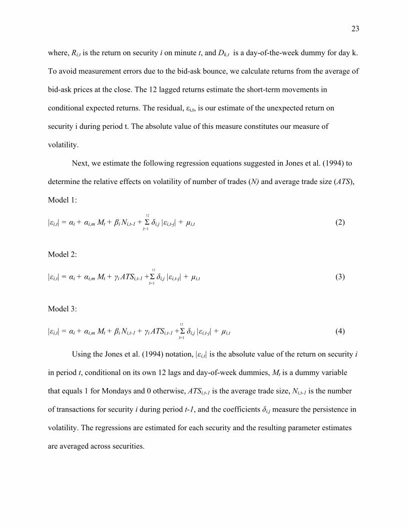
where, Ri,t is the return on security i on minute t, and Dk,t is a day-of-the-week dummy for day k.

To avoid measurement errors due to the bid-ask bounce, we calculate returns from the average of

bid-ask prices at the close. The 12 lagged returns estimate the short-term movements in

conditional expected returns. The residual, εi,t, is our estimate of the unexpected return on

security i during period t. The absolute value of this measure constitutes our measure of

volatility.

Next, we estimate the following regression equations suggested in Jones et al. (1994) to

determine the relative effects on volatility of number of trades (N) and average trade size (ATS),

Model 1:

12

|εi,t| = αi + αi,m Mt + βi Ni,t-1 + Σ δi,j |εi,t-j| + µi,t (2) J=1

Model 2:

12

|εi,t| = αi + αi,m Mt + γi ATSi,t-1 +Σ δi,j |εi,t-j| + µi,t (3) J=1

Model 3:

12 |εi,t| = αi + αi,m Mt + βi Ni,t-1 + γi ATSi,t-1 +Σ δi,j |εi,t-j| + µi,t (4) J=1

Using the Jones et al. (1994) notation, |εi,t| is the absolute value of the return on security i

in period t, conditional on its own 12 lags and day-of-week dummies, Mt is a dummy variable

that equals 1 for Mondays and 0 otherwise, ATSi,t-1 is the average trade size, Ni,t-1 is the number

of transactions for security i during period t-1, and the coefficients δi,j measure the persistence in

volatility. The regressions are estimated for each security and the resulting parameter estimates

are averaged across securities.

24

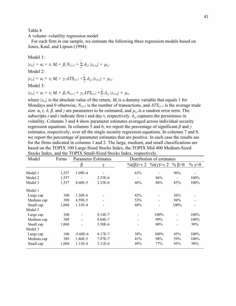
Table 8 summarizes the result for the three models. Table 8, Panel A, provides the results

from the estimation of regression Eqs. (2)– (4) using the high frequency, minute by minute

returns for all securities in our sample. Overall, our results are contrary to the results in Jones et

al. (1994). The explanatory power of Model 2, where volume is measured by the average trade

size, is stronger than the explanatory power of Model 1, where volume is measured by the

average number of trades. Moreover, the average number of trades has little marginal

explanatory power when volatility is conditioned on the average trade size in Model 3. In Model

3, 84% of the coefficients for the average trade size are statistically significant, and 100% of the

significant coefficients for the average trade size are greater than zero. Comparable results for

the number of trades are 46% and 85%, respectively.

We re-estimate the three regression models for the three different size portfolios. The

results from these estimations are presented in Table 8, Panel B. In general, the results from

estimating separate regression models for each size portfolio are similar to the results from

estimating one regression for the whole sample. However, the results are stronger for large- and

mid-cap stocks with almost 100% of the coefficients for the average trade size are statistically

positively significant at the 5% level of significance while, 77% of the coefficients for average

trade size are significantly positive for small-cap firms.

Hence, our results show that the average trade size is the dominant factor determining the

volume-volatility relation in the Japanese market, which directly contradicts the findings of

Jones et. al. (1994) for U.S. markets and Naes and skeljtorp (2006) for Norwegian markets. But

our results support the findings of Grundy and McNicholas (1989).

25

5.8. The predictive power of cost-to-buy versus cost-to-sell

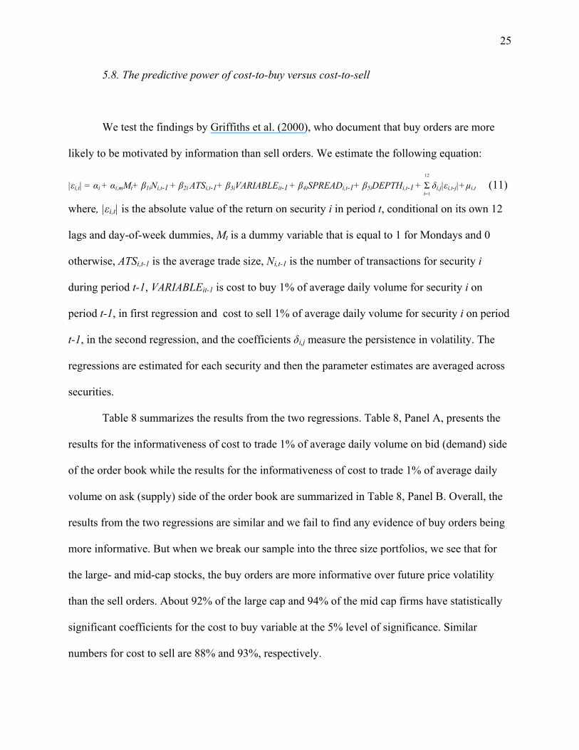
We test the findings by Griffiths et al. (2000), who document that buy orders are more

likely to be motivated by information than sell orders. We estimate the following equation:

12

|εi,t| = αi + αi,mMt+ β1iNi,t-1 + β2i ATSi,t-1+ β3iVARIABLEit-1 + β4iSPREADi,t-1+ β5iDEPTHi,t-1 + Σ δi,j|εi,t-j|+µi,t (11) J=1

where, |εi,t| is the absolute value of the return on security i in period t, conditional on its own 12

lags and day-of-week dummies, Mt is a dummy variable that is equal to 1 for Mondays and 0

otherwise, ATSi,t-1 is the average trade size, Ni,t-1 is the number of transactions for security i

during period t-1, VARIABLEit-1 is cost to buy 1% of average daily volume for security i on

period t-1, in first regression and cost to sell 1% of average daily volume for security i on period

t-1, in the second regression, and the coefficients δi,j measure the persistence in volatility. The

regressions are estimated for each security and then the parameter estimates are averaged across

securities.

Table 8 summarizes the results from the two regressions. Table 8, Panel A, presents the

results for the informativeness of cost to trade 1% of average daily volume on bid (demand) side

of the order book while the results for the informativeness of cost to trade 1% of average daily

volume on ask (supply) side of the order book are summarized in Table 8, Panel B. Overall, the

results from the two regressions are similar and we fail to find any evidence of buy orders being

more informative. But when we break our sample into the three size portfolios, we see that for

the large- and mid-cap stocks, the buy orders are more informative over future price volatility

than the sell orders. About 92% of the large cap and 94% of the mid cap firms have statistically

significant coefficients for the cost to buy variable at the 5% level of significance. Similar

numbers for cost to sell are 88% and 93%, respectively.

26

Finally, we analyze the predictive power of liquidity for predicting the trading speed.

Based on the results summarized in table 10, we find that cost based liquidity measure have

stronger predictive power than the elasticity based measure. The predictive power of cost-to-

trade is stronger for medium cap and larger cap stocks than for small cap stocks.

6. Robustness check

We perform additional robustness tests for the results presented in the above section.

Since, our sample have unequal numbers of stocks in each of the three size categories, we re-

analyze the results by selecting the top 40 firms based on market capitalization for each of the

three size portfolios. By conducting this further analysis, we find even stronger results that are

consistent with the ones presented in the above section.

We have presented the results for minute-by-minute analysis of the LOB. In unreported

results, we conducted a quote-by-quote analysis and also analyses based on 5 minutes and 30

minutes snapshot of the LOB. The results are similar to those reported for the 1 minute analysis.

However, the results based on 30 minute snapshots are not as strong for large-cap stocks as

found for the minute-by-minute analysis.

6. Conclusion

We examine the information content of the various liquidity measures in explaining

future price volatility in the TSE. We also investigate whether average trade size or number of

trades is the dominant factor in explaining the volume-volatility relationship. Finally, we analyze

27

the predictive power of LOB liquidity for predicting the future trading price movements and

trading speed.

To study different dimensions of the LOB and the liquidity, we use the dispersion and

cost-to-trade measures as the proxy of the tightness and depth of the book (Kang and Yeo, 2008).

We also analyze the informativeness of order book slope over future price volatility to determine

whether we support the Naes and Skeljtorp (2006) finding of a negative relationship between

informativeness and future price volatility. We also construct a new measure, proportion of

average daily volume executed within the 3 ticks of the mid-quote, which captures the market

depth around the mid-quote.

Analyzing the stocks included in the TOPIX index, we find that the cost to trade 1% of

average daily volume is the dominant liquidity measure that significantly and consistently

predicts future price volatility on the Tokyo Stock Exchange. The higher the cost to trade 1% of

average daily volume, the higher the future price volatility. We also find that the order book

slope is informative in explaining future price volatility for the majority of large- and mid-cap

stocks. This result supports the findings of Naes and Skeljtorp (2006) and Duong and Kalev

(2009) that the gentler the slope, the higher the price volatility. But we do not find significant

predictive power for order book slope in the case of small-cap firms.

We find a significant relation between dispersion of orders and future price volatility for

small-cap stocks, but not for large- and mid-cap stocks. The lower the dispersion of the LOB, the

lower is the future price volatility. Quoted spread failed to predict future price volatility. Hence,

our results contradict the findings of Booth & Gurun (2008), Kalimipalli & Warga (2002) and

Hasbrouck (1999), who find a significantly positive relationship between spread and future price

volatility. We find that buy orders are slightly more informative than the sell orders for the large-

28

and mid-cap firms, but not for small-cap stocks. Hence, we find support for Burdett and O'Hara’s

(1987) and Griffiths et al. (2000).

We also find support for Grundy and McNichols’s (1989) conclusion that informed

traders prefer to trade large amounts at any given price. We find that average trade size, and not

number of trades, is the dominant determinant of the volume–volatility relationship.

Finally, we document that LOB liquidity can significantly predict future trade price

movements and trading speed. Cost based liquidity measures do a better job of predicting future

price changes. These results can prove useful to traders in formulating their trading strategies.

29

References

Admati, A., Pfleiderer, P., 1988. A theory of intraday patterns: volume and price variability. Review of Financial Studies 1, 3-40.

Ahn H-J., Bae K-H. and Chan K., 2001, Limit Orders, Depth and Volatility: Evidence from the Stock Exchange of Hong Kong, Journal of Finance, 56, 767-788.

Amihud, Y. 2002. Illiquidity and Stock Returns: Cross-Section and Time-Series Effects. Journal of Financial Markets 5: 31–56.

Amihud, Y. and H. Mendelson. 1986. Asset Pricing and the Bid-ask Spread. Journal of Financial Economics 17: 223–249.

Ascioglu A, C. Comerton-Forde and T. McInish, 2007, Price clustering on the Tokyo Stock Exchange, Financial Review 42(2), 289-301.

Bollerslev, T., Melvin, M., 1994. Bid-ask spreads and the volatility in the foreign exchange market. Journal of International Economics 36, 355 – 372.

Booth, G.G., Gurun, U.G., 2008. Volatility clustering and the bid–ask spread: exchange rate behavior in early renaissance Florence. Journal of Empirical Finance 15 (1), 131–144.

Brennan, M. and A. Subrahmanyam. 1996. Market Microstructure and Asset Pricing: On the Compensation for Illiquidity in Stock Returns. Journal of Financial Economics 41: 441–464.

Brennan, M., T. Chordia and A. Subrahmanyam. 1998. Alternative Factor Specifications, Security Characteristics, and the Cross-Section of Expected Stock Returns. Journal of Financial Economics 49: 345–373.

Burdett, K., O’Hara, M., 1987. Building blocks, an introduction to block building. Journal of Banking and Finance 11, 193-212. Chakravarty, S., Holden, C., 1995. An integrated model of market and limit orders. Journal of

Financial Intermediation 4, 213-241. Chan, K., & Fong, W., 2000. Trade size, order imbalance, and the volatility–volume relation.

Journal of Financial Economics 57, 247–273. Chan, K., & Fong, W., 2006. Realized volatility and transactions. Journal of Banking and

Finance 30, 2063–2085. Chung, K., Van Ness, B., & Van Ness, R. (1999). Limit orders and the bid-ask spread. Journal of

Financial Economics, 53 (2), 255-287. Copeland, T., Galai, D., 1983. Information effects and the bid-ask spreads. Journal of Finance

38, 1457-1469. Duong, H.N., Kalev, P.S., Krishnamurti, C., 2008. Order aggressiveness of institutional and

individual investors. Working paper, Monash University. Duong, H.N., Kalev, P.S., 2009. Order Book Slope and Price Volatility. Working paper, Monash

University. Fleming, J., Kirby, C., Ostdiek, B., 2003. The economic value of volatility timing using “realized

volatility”. Journal of Financial Economics 67, 473-509. Foucault, T., Moinas, S., Theissen, E., 2007. Does anonymity matter in electronic limit order

markets? Review of Financial Studies 20, 1707-1747. Foucault, T., 1999. Price formation in a dynamic limit order market. Journal of Financial

Markets 2, 99-134. Giot, P., Laurent S., & Petitjean, M., 2009. Trading activity, realized volatility and jumps,

Journal of Empirical Finance, doi:10.1016/j.jempfin.2009.07.001

30

Glosten, L., Milgrom, P., 1985. Bid, ask and transaction prices in a specialist market with heterogeneously informed traders. Journal of Financial Economics 14, 71–100.

Goldstein, M.A., Kavajecz, K.A., 2004. Trading strategies during circuit breakers and extreme market movements. Journal of Financial Markets 7, 301–333.

Griffiths, M.D., Smith, B., Turnbull, D.A.S., White, R.W., 2000. The costs and determinants of order aggressiveness. Journal of Financial Economics 56, 65-88.

Grundy, B., McNichols, M., 1989. Trade and revelation of information through prices and direct disclosure. Review of Financial Studies 2, 495-526.

Hasbrouck, J., 1999. The dynamics of discrete bid and ask quotes. Journal of Finance 54, 2109 – 2142.

Hasbrouck, J., Saar, G., 2002. Limit orders and volatility in a hybrid market: The Island ECN. Working paper, Stern Business School, New York University.

Higgs, H., Worthington, A., 2008. Stochastic price modelling of high volatility, meanreverting, spike-prone commodities: The Australian wholesale spot electricity market. Energy Economics 30 (6), 3172–3185.

Holthausen, R., Verrecchia, R., 1990. The effect of informedness and consensus on price and volume behavior. Accounting Review 65, 191-208.

Huang, R.D., Masulis, R.W., 2003. Trading activity and stock price volatility: evidence from the London Stock Exchange. Journal of Empirical Finance 10, 249–269.

Jacoby, G., D. Fowler and A. Gottesman. 2000. The Capital Asset Pricing Model and the Liquidity Effect: A Theoretical Approach. Journal of Financial Markets 3: 69–81.

Jones, C. 2001.ACentury of Stock Market Liquidity and Trading Costs. Working Paper, Columbia University, New York.

Jones, C., Kaul, G., Lipson, M., 1994. Transactions, volume and volatility. Review of Financial Studies 7, 631–651.

Kalimipalli, M., Warga, A., 2002. Bid-ask spread, volatility, and volume in the corporate bond market. Journal of Fixed Income (March), 31 – 42.

Kaniel, R., Liu, H., 2006. So what orders do informed traders use? Journal of Business 79, 1867-1914.

Kim, O., Verrecchia, R., 1991. Market reactions to anticipated announcements. Journal of Financial Economics 30, 273-310.

Kyle, A., 1985. Continuous auctions and insider trading. Econometrica 53, 1315-1335. Naes, R., Skjeltorp, J.A., 2006. Order book characteristics and the volume-volatility relation:

Empirical evidence from a limit order market. Journal of Financial Markets 9, 408-432. Pascual, R., Veredas, D., 2006. Does the open limit order book matter in explain long run

volatility? Working paper, Universidad de las Islas Baleares. Rahman, S., Lee, C. F., & Ang, K. P. (2002). Intraday return volatility process: Evidence from

NASDAQ stocks. Review of Quantitative Finance and Accounting, 19, 155-180. TSE Annual Report, 2009. Retrieved on November 27, 2009 from

http://www.tse.or.jp/english/about/ir/financials/annual/annual_2009.pdf Wald, J.K., Horrigan, H.T., 2005. Optimal limit order choice. Journal of Business 78, 597-619.

31

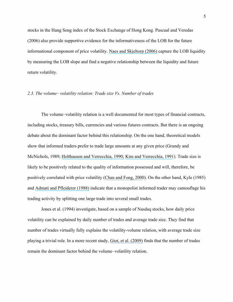
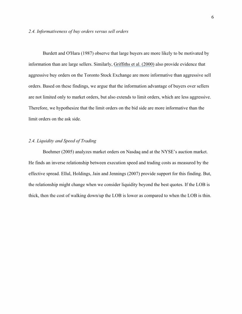
Figure 1. Examples of two order books. The figure shows the total and visible order books of two large Japanese firms, averaged over the trading days of June 2008. The picture to the left is the order book of Nissan Motor Co. Ltd., a traditional automobile manufacturer, while the right picture is the order book of Dream Incubator Inc., a relatively new firm in incubation business. The vertical axis shows the cumulative percentage share volume in the book, and the horizontal axis shows ticks away from the quotes. 1 and -1 represent the best ask and bid quote, respectively.

0

20

40

60

80

100

120

-10 -5 0 5 10

Acc

umul

ated

% V

olum

e

Bid Side<------ Tick ----->Ask Side

NISSAN MOTOR CO.LTD.

0

20

40

60

80

100

120

-10 -5 0 5 10

Acc

umul

ated

% V

olum

e

Bid Side<------ Tick ----->Ask Side

Dream Incubator Inc.

32

Table 1 Descriptive statistics We present statistics for all firms by market capitalization for the period 1 July 2007 to 30 June 2008. For each firm, at the end of each minute of trading, we calculate the slope for the five best bids (BIDSLOPE) and five best asks (ASKSLOPE), using Eqs. (1) and (2), in turn. SLOPE is the average of BIDSLOPE and ASKSLOPE. We calculate the following variables for each firm. SPREAD is the mean spread over each minute of trading. DEPTH is the sum of the depth at the best bid and best ask at the end of each minute of trading. DISDT and DISSP are the dispersion of limit orders and the dispersion from the Best Quotes that measure the distance between the orders and between the orders and the best quotes, respectively. Cost-to-tradeXX measures the cost that liquidity demanders have to bear above the intrinsic value due to a sudden surge in the demand of liquidity where XX is 1%, 0.1% and 0.01%, in turn, of the daily average trading volume. We also calculate the Cost-to-trade measure for trading 100 and 1000 stocks per minute of trading. Finally, we calculate the number of trades (N) and the average trade size (ATS) for each minute of trading. We present the mean values for each variable across firms for all firms together, and for large, medium, and small firms, classified by market capitalization. The large, medium, and small classifications are based on the TOPIX 100 Large-Sized Stocks Index, the TOPIX Mid400 Medium-Sized Stocks Index, and the TOPIX Small-Sized Stocks Index, respectively. Market capitalization All firms

(n = 1,557) Large

(n = 100) Medium (n = 389)

Small (n = 1,068)

SLOPE 15.10 25.55 19.75 11.00 ASKSLOPE 15.01 25.50 19.70 10.94 BIDSLOPE 15.05 25.60 19.80 10.93 SPREAD 0.36 0.19 0.24 0.45 DEPTH 56,789 82,594 58,350 51,080 COSTTOTRD1% 0.0057 0.0041 0.0042 0.0067 COSTTOBUY1% 0.0029 0.0020 0.0021 0.0034 COSTTOSELL1% 0.0028 0.0021 0.0021 0.0034 COSTTOTRD0.1% 0.0037 0.0021 0.0024 0.0047 COSTTOTRD0.01% 0.0036 0.0019 0.0023 0.0045 COSTTOTRD100 0.0042 0.0020 0.0024 0.0056 COSTTOTRD1000 0.0060 0.0027 0.0032 0.0080 DISDT 55.56 31.29 38.78 267.35 DISSP -0.11 -6.44 -1.00 1.26 N 1.81 4.64 2.28 1.17 ATS 1,605 4,813 2,285 790

33

Table 2 Predicting future trade price movements using liquidity measures For each firm in our sample, we estimate the following regression model: PRIi,t = αi + αib BIDLIQUIDITYit-j + αia ASKLIQUIDITYit-j + µi,t

where PRIi,t is the magnitude of the trade price change. We calculate Elasticity based liquidity measures, slope for the five best bids (BIDSLOPE) and five best asks (ASKSLOPE), using Eqs. (1) and (2), in turn, for each firm, for every change in LOB. We also calculate cost based liquidity measures, cost that liquidity demanders have to bear to buy 1% of the daily average trading volume, CTSELLi,t-1 is the cost that liquidity demanders have to bear to sell 1% of the daily average trading volume. is the change operator. α are parameters to be estimated, and µi,t is a random error term. The subscripts i and t indicate firm i and period t, respectively. Panels A and C present the results for predicting the next trade price changes based on lagged LOB information. Panels B and D present the results for predicting the second trade price changes based on lagged LOB information. Panel E presents the results for predicting the trade price changes based on the previous minute’s LOB information. Panel F presents the results for predicting the trade price changes based on 2 minutes prior to the trade LOB information. Columns 2 and 5 present the parameter estimates averaged across all individual security regression equations, columns 3 and 6 report the percentage of significant β estimates and columns 4 and 6 report the percentage of parameter estimates that are positive. The large, medium, and small classifications are based on the TOPIX 100 Large-Sized Stocks Index, the TOPIX Mid 400 Medium-Sized Stocks Index, and the TOPIX Small-Sized Stocks Index, respectively. Panel A. Predicting the next trade price movement based on Elasticity based Liquidity Measures PRIDIFFi,t = αi + αib BIDSLOPEit-1 + αia ASKSLOPEit-1 + µi,t

BID SLOPE ASK SLOPE

Variables (αis) t(αis)>±2 αis>0 (αic) t(αic)>±2 αic>0

All Firms 0.011 80% 100% -0.013 77% 0%

Large-Cap 0.017 87% 100% -0.017 79% 1%

Medium-Cap 0.004 87% 100% -0.004 84% 0%

Small-Cap 0.012 77% 100% -0.016 76% 0%

Panel B. Predicting the second trade price movement based on Elasticity based Liquidity Measures PRIDIFFi,t = αi + αib BIDSLOPEit-2 + αia ASKSLOPEit-2 + µi,t

BID SLOPE ASK SLOPE

Variables (αis) t(αis)>±2 αis>0 (αic) t(αic)>±2 αic>0

All Firms 0.052 19% 94% -0.046 18% 9%

Large-Cap 0.001 14% 79% 0.011 16% 50%

Medium-Cap 0.004 24% 93% -0.004 22% 9%

Small-Cap 0.080 17% 96% -0.072 17% 6%

34

Table 2--continued Panel C. Predicting the next trade price movement based on Cost based Liquidity Measures PRIDIFFi,t = αi + αib BIDCTTit-1 + αia ASKCTTit-1 + µi,t

BID COST-TO-TRADE ASK COST-TO-TRADE

Variables (αis) t(αis)>±2 αis>0 (αic) t(αic)>±2 αic>0

All Firms -3.24 78% 2% 2.22 73% 99%

Large-Cap -15.32 81% 0% 16.11 74% 100%

Medium-Cap -10.02 84% 0% 4.90 77% 100%

Small-Cap -2.78 76% 3% 1.70 72% 98%

Panel D. Predicting the second trade price movement based on Cost based Liquidity Measures PRIDIFFi,t = αi + αib BIDCTTit-2 + αia ASKCTTit-2 + µi,t

BID COST-TO-TRADE ASK COST-TO-TRADE

Variables (αis) t(αis)>±2 αis>0 (αic) t(αic)>±2 αic>0

All Firms -5.25 33% 10% 10.99 31% 91%

Large-Cap -18.97 31% 13% 18.80 24% 80%

Medium-Cap -4.84 37% 4% 4.89 37% 93%

Small-Cap -1.17 37% 19% 17.90 29% 90%

Panel D. Calendar time forecasting using Elasticity based Liquidity Measure (minute-by-minute snapshot) PRIDIFFi,t = αi + αib BIDSLOPEit-1 + αia ASKSLOPEit-1 + µi,t

BID SLOPE ASK SLOPE

Variables (αis) t(αis)>±2 αis>0 (αic) t(αic)>±2 αic>0

All Firms 0.008 67% 100% -0.002 63% 0%

Large-Cap 0.012 58% 100% -0.010 61% 0%

Medium-Cap 0.004 71% 100% -0.001 62% 1%

Small-Cap 0.010 67% 100% -0.003 64% 1%

35

Table 2--continued Panel E. Calendar time forecasting using Elasticity based Liquidity Measure (2 minute snapshot) PRIDIFFi,t = αi + αib BIDSLOPEit-2 + αia ASKSLOPEit-2 + µi,t

BID SLOPE ASK SLOPE

Variables (αis) t(αis)>±2 αis>0 (αic) t(αic)>±2 αic>0

All Firms 0.091 12% 88% -0.001 11% 11%

Large-Cap 0.148 10% 90% -0.008 4% 25%

Medium-Cap 0.005 13% 84% -0.001 13% 8%

Small-Cap 0.001 12% 90% -0.001 11% 11%

Panel F. Calendar time forecasting using Cost based Liquidity Measure (minute by minute snapshot) PRIDIFFi,t = αi + αib BIDCTTit-1 + αia ASKCTTit-1 + µi,t

BID COST-TO-TRADE ASK COST-TO-TRADE

Variables (αis) t(αis)>±2 αis>0 (αic) t(αic)>±2 αic>0

All Firms -23.75 61% 2% 20.91 62% 99%

Large-Cap -45.55 51% 4% 24.41 47% 100%

Medium-Cap -9.95 58% 1% 9.19 58% 99%

Small-Cap -14.41 64% 3% 14.72 65% 98%

Panel G. Calendar time forecasting using Cost based Liquidity Measure (2 minute snapshot) PRIDIFFi,t = αi + αib BIDCTTit-2 + αia ASKCTTit-2 + µi,t

BID COST-TO-TRADE ASK COST-TO-TRADE

Variables (αis) t(αis)>±2 αis>0 (αic) t(αic)>±2 αic>0

All Firms -10.41 25% 15% 13.84 25% 87%

Large-Cap -24.01 12% 0% 5.57 15% 87%

Medium-Cap -5.97 29% 10% 8.51 30% 92%

Small-Cap -18.04 25% 18% 2.17 24% 85%

36

Table 3 A spread–volatility regression model For each firm in our sample, we estimate the following two regression models: Model 1: 12 |εi,t| = αi + αi,m Mt + β1i Ni,t-1 + β2i ATSi,t-1 + β3i SPREADi,t-1 + Σ δi,j |εi,t-j| + µi,t J=1 Model 2: 12 |εi,t| = αi + αi,m Mt + β1i Ni,t-1 + β2i ATSi,t-1 + β3i SPREADi,t-1 + β4i DEPTHi,t-1 + Σ δi,j |εi,t-j| + µi,t J=1 where |εi,t| is the absolute value of the return, conditional on its own 12 lags and day-of-week dummies, Mt is a dummy variable that is equal to 1 for Mondays and 0 otherwise, Ni,t-1 is the number of transactions, ATSi,t-1 is the average trade size, SPREADi,t-1 is the mean spread and DEPTHi,t-1 is the sum of depth at the best bid and best ask quotes. α, β, and δ are parameters to be estimated, and µi,t is a random error term. The subscripts i and t indicate firm i and day t, respectively. δi,j captures the persistence in volatility. Columns 2 and 5 present the parameter estimates averaged across all individual security regression equations, columns 3 and 6 report the percentage of significant β estimates and columns 4 and 7 reports the percentage of parameter estimates that are positive. The first part of the table presents the results from running the regression equations over the whole sample. The second part of the table reports the results from splitting the sample into three size based portfolios. The large, medium, and small classifications are based on the TOPIX 100 Large-Sized Stocks Index, the TOPIX Mid 400 Medium-Sized Stocks Index, and the TOPIX Small-Sized Stocks Index, respectively.

Model 1 Model 2

Variables (β) t(β)>± 2 β>0 (β) t(β)>± 2 β>0 M 1.46E-4 9% 92% 1.24E-4 9% 90% N 8.27E-5 45% 83% 8.84E-5 45% 86% ATS 2.09E-6 84% 100% 2.09E-6 84% 100% SPREAD 6.42E-4 66% 71% 4.48E-8 55% 72% DEPTH - - - 7.11E-4 65% 74%

Large Cap Medium Cap Small Cap Variables (β) t(β)>± 2 β>0 (β) t(β)>± 2 β>0 (β) t(β)>± 2 β>0 M 3.95E-5 9% 78% 5.80E-5 9% 88% 1.56E-4 9% 91% N -6.01E-6 37% 43% 1.98E-5 39% 61% 1.12E-4 48% 96% ATS 7.99E-7 100% 100% 7.87E-7 98% 100% 2.85E-6 77% 99% SPREAD -1.06E-8 70% 66% 1.89E-8 66% 67% 6.46E-8 50% 75% DEPTH 2.01E-3 84% 86% 9.77E-4 76% 91% 4.14E-4 59% 64%

37

Table 4 A dispersion–volatility regression model For each firm in our sample, we estimate the following regression model: 12 |εi,t| = αi+αi,m Mt+ β1i Ni,t-1+ β2i ATSi,t-1+ β3i DISDTit-1+ β4i SPREADi,t-1+ β5i DEPTHi,t-1+ Σ δi,j |εi,t-j|+ µi,t J=1 where |εi,t| is the absolute value of the return, conditional on its own 12 lags and day-of-week dummies, Mt is a dummy variable that is equal to 1 for Mondays and 0 otherwise, Ni,t-1 is the number of transactions, ATSi,t-1 is the average trade size, DISDTi,t-1 is the dispersion of limit orders, SPREADi,t-1 is the mean spread and DEPTHi,t-1 is the sum of depth at the best bid and best ask quotes. α, β, and δ are parameters to be estimated, and µi,t is a random error term. The subscripts i and t indicate firm i and day t, respectively. δi,j captures the persistence in volatility. Column 2 presents the parameter estimates averaged across all individual security regression equations, column 3 reports the percentage of significant β estimates and column 4 reports the percentage of parameter estimates that are positive. The first part of the table presents the results from running the regression equations over the whole sample. The second part of the table reports the results from splitting the sample into three size based portfolios. The large, medium, and small classifications are based on the TOPIX 100 Large-Sized Stocks Index, the TOPIX Mid 400 Medium-Sized Stocks Index, and the TOPIX Small-Sized Stocks Index, respectively. Variables Estimate (β) %t(β)>± 2 % β>0 M 1.07E-4 8% 86% N 8.65E-5 46% 87% ATS 1.84E-6 83% 100% DISDT 3.41E-4 74% 82% SPREAD 5.67E-4 72% 52% DEPTH 1.68E-7 54% 74%

Large Cap Medium Cap Small Cap Variables (β) t(β)>± 2 β>0 (β) t(β)>± 2 β>0 (β) t(β)>± 2 β>0 M 2.82E-5 10% 70% 4.42E-5 8% 79% 1.36E-4 8% 90% N 9.96E-7 35% 63% 2.13E-5 41% 64% 1.13E-4 48% 96% ATS 8.00E-7 100% 100% 7.86E-7 98% 100% 2.47E-6 75% 100% DISDT -5.41E-4 82% 21% -1.66E-4 78% 60% 6.36E-4 72% 97% SPREAD 2.75E-3 95% 90% 1.01E-3 84% 72% 5.88E-5 65% 37% DEPTH -2.72E-8 82% 34% 2.26E-8 68% 59% 2.78E-7 47% 88%

38

Table 5 A Slope–volatility regression model For each firm in our sample, we estimate the following regression model: 12 |εi,t| = αi + αi,m Mt +β1i Ni,t-1+ β2i ATSi,t-1+ β3i SLOPEit-1+β4i SPREADi,t-1+β5i DEPTHi,t-1+Σ δi,j |εi,t-j| + µi,t J=1 where |εi,t| is the absolute value of the return, conditional on its own 12 lags and day-of-week dummies, Mt is a dummy variable that is equal to 1 for Mondays and 0 otherwise, Ni,t-1 is the number of transactions, ATSi,t-1 is the average trade size, SLOPEi,t-1 is the average of slope for the five best bids and five best asks, SPREADi,t-1 is the mean spread and DEPTHi,t-1 is the sum of depth at the best bid and best ask quotes. α, β, and δ are parameters to be estimated, and µi,t

is a random error term. The subscripts i and t indicate firm i and day t, respectively. δi,j captures the persistence in volatility. Column 2 presents the parameter estimates averaged across all individual security regression equations, column 3 reports the percentage of significant β estimates and column 4 reports the percentage of parameter estimates that are positive. The first part of the table presents the results from running the regression equations over the whole sample. The second part of the table reports the results from splitting the sample into three size based portfolios. The large, medium, and small classifications are based on the TOPIX 100 Large-Sized Stocks Index, the TOPIX Mid 400 Medium-Sized Stocks Index, and the TOPIX Small-Sized Stocks Index, respectively. Variables Estimate (β) %t(β)>± 2 % β>0 M 8.33E-5 9% 70% N 8.52E-5 45% 82% ATS 2.43E-6 84% 100% SLOPE -4.05E-6 86% 25% SPREAD -9.09E-4 48% 41% DEPTH 9.59E-6 39% 71%

Large Cap Medium Cap Small Cap Variables (β) t(β)>± 2 β>0 (β) t(β)>± 2 β>0 (β) t(β)>± 2 β>0 M -9.77E-6 12% 50% 1.36E-5 9% 61% 1.21E-4 9% 76% N -5.42E-6 42% 43% 1.54E-5 45% 53% 1.18E-4 46% 95% ATS 7.96E-7 100% 100% 9.82E-7 99% 100% 3.31E-6 78% 99% SLOPE -1.27E-6 82% 13% -1.06E-6 75% 9% -6.23E-6 46% 37% SPREAD 4.78E-4 77% 56% -1.34E-3 59% 28% -9.27E-4 42% 45% DEPTH 5.18E-8 50% 70% 4.29E-8 61% 84% 1.81E-5 30% 61%

39

Table 6 A cost-to-trade–volatility regression model For each firm in our sample, we estimate the following regression model: 12 |εi,t| =αi+αi,mMt+β1iNi,t-1+β2iATSi,t-1+β3iCOSTTRADEit-1+β4iSPREADi,t-1+β5iDEPTHi,t-1+Σδi,j|εi,t-j|+µi,t J=1 where |εi,t| is the absolute value of the return, conditional on its own 12 lags and day-of-week dummies, Mt is a dummy variable that is equal to 1 for Mondays and 0 otherwise, Ni,t-1 is the number of transactions, ATSi,t-1 is the average trade size, COSTTRADEi,t-1 is the cost that liquidity demanders have to bear to trade 1% of the daily average trading volume, SPREADi,t-1

is the mean spread and DEPTHi,t-1 is the sum of depth at the best bid and best ask quotes. α, β, and δ are parameters to be estimated, and µi,t is a random error term. The subscripts i and t indicate firm i and day t, respectively. δi,j captures the persistence in volatility. Column 2 presents the parameter estimates averaged across all individual security regression equations, column 3 reports the percentage of significant β estimates and column 4 reports the percentage of parameter estimates that are positive. The first part of the table presents the results from running the regression equations over the whole sample. The second part of the table reports the results from splitting the sample into three size based portfolios. The large, medium, and small classifications are based on the TOPIX 100 Large-Sized Stocks Index, the TOPIX Mid 400 Medium-Sized Stocks Index, and the TOPIX Small-Sized Stocks Index, respectively. Variables Estimate (β) %t(β)>± 2 % β>0 M 8.53E-5 9% 82% N 8.65E-5 48% 84% ATS 1.79E-6 86% 98% COSTTOTRD 0.20 92% 97% SPREAD -1.80E-3 73% 73% DEPTH 3.00E-7 65% 93%

Large Cap Medium Cap Small Cap Variables (β) t(β)>±2 β>0 (β) t(β)>±2 β>0 (β) t(β)>±2 β>0 M 3.08E-5 8% 75% 4.69E-5 9% 82% 1.02E-4 10% 83% N 9.96E-7 35% 34% 2.13E-5 36% 59% 1.13E-4 54% 93% ATS 7.96E-7 100% 100% 7.85E-7 98% 100% 2.36E-6 80% 97% COSTTOTRD 0.11 92% 97% 0.10 98% 100% 0.25 90% 96% SPREAD 1.12E-3 80% 75% -2.86E-4 66% 41% -2.59E-3 74% 18% DEPTH 1.66E-8 80% 89% 5.32E-8 73% 96% 4.43E-7 61% 92%

40

Table 7 A liquidity–volatility regression model For each firm in our sample, we estimate the following regression model:

|εi,t| = αi+αi,mMt+β1i Ni,t-1+β2i ATSi,t-1+β3i DISDTi,t-1+β4iSLOPEit-1+β5iCOSTTRADEi,t-1+ β6iSPREADi,t-1 12

+β7i DEPTHi,t-1+Σ δi,j|εi,t-j|+µi,t J=1 where |εi,t| is the absolute value of the return, conditional on its own 12 lags and day-of-week dummies, Mt is a dummy variable that is equal to 1 for Mondays and 0 otherwise, Ni,t is the number of transactions, ATSi,t-1 is the average trade size, DISDTi,t-1 is the dispersion of limit orders, SLOPEi,t-1 is the average of slope for the five best bids and five best asks, COSTTRADEi,t-1 is the cost that liquidity demanders have to bear to trade 1% of the daily average trading volume, SPREADi,t-1 is the mean spread and DEPTHi,t-1 is the sum of depth at the best bid and best ask quotes. α, β, and δ are parameters to be estimated, and µi,t is a random error term. The subscripts i and t indicate firm i and day t, respectively. δi,j captures the persistence in volatility. Column 2 presents the parameter estimates averaged across all individual security regression equations, column 3 reports the percentage of significant β estimates and column 4 reports the percentage of parameter estimates that are positive. The first part of the table presents the results from running the regression equations over the whole sample. The second part of the table reports the results from splitting the sample into three size based portfolios. The large, medium, and small classifications are based on the TOPIX 100 Large-Sized Stocks Index, the TOPIX Mid 400 Medium-Sized Stocks Index, and the TOPIX Small-Sized Stocks Index, respectively. Variables Estimate (β) %t(β)>± 2 % β>0 VIF M 4.32E-5 12% 62% 0.89 N 8.16E-5 50% 82% 3.36 ATS 2.37E-6 88% 98% 1.91 DISDT 3.26E-4 67% 83% 0.68 SLOPE -1.77E-7 49% 28% 3.48 COSTTOTRD 0.22 85% 99% 4.67 DEPTH 4.02E-8 45% 81% 4.23

Large Cap Medium Cap Small Cap Variables (β) t(β)>±2 β>0 (β) t(β)>±2 β>0 (β) t(β)>±2 β>0 M -2.14E-5 13% 38% 8.81E-6 9% 60% 5.76E-5 13% 65% N -3.73E-6 42% 48% 1.91E-5 41% 57% 1.05E-4 54% 91% ATS 7.98E-7 100% 100% 9.82E-7 99% 100% 3.15E-6 84% 96% DISDT -4.73E-4 63% 21% -2.61E-4 62% 57% 5.86E-4 69% 96% SLOPE -1.15E-6 61% 11% -4.00E-7 56% 8% 4.59E-8 45% 63% COSTTOTRD 0.09 81% 98% 0.09 88% 99% 0.27 85% 100% DEPTH 3.11E-8 52% 58% 5.24E-8 62% 87% 3.41E-8 38% 80%

41

Table 8 A volume–volatility regression model For each firm in our sample, we estimate the following three regression models based on Jones, Kaul, and Lipson (1994): Model 1: 12

|εi,t| = αi + τi Mt + βi Ni,t-1 + Σ δi,j |εi,t-j| + µi,t J=1

Model 2: 12 |εi,t| = αi + τi Mt + γi ATSi,t-1 +Σ δi,j |εi,t-j| + µi,t J=1 Model 3: 12 |εi,t| = αi + τi Mt + βi Ni,t-1 + γi ATSi,t-1 +Σ δi,j |εi,t-j| + µi,t J=1 where |εi,t| is the absolute value of the return, Mt is a dummy variable that equals 1 for Mondays and 0 otherwise, Ni,t-1 is the number of transactions, and ATSi,t-1 is the average trade size. α, τ, δ, β, and γ are parameters to be estimated, and µi,t is a random error term. The subscripts i and t indicate firm i and day t, respectively. δi,j captures the persistence in volatility. Columns 3 and 4 show parameter estimates averaged across individual security regression equations. In columns 5 and 6, we report the percentage of significant β and γ estimates, respectively, over all the single security regression equations. In columns 7 and 8, we report the percentage of parameter estimates that are positive. In each case the results are for the firms indicated in columns 1 and 2. The large, medium, and small classifications are based on the TOPIX 100 Large-Sized Stocks Index, the TOPIX Mid 400 Medium-Sized Stocks Index, and the TOPIX Small-Sized Stocks Index, respectively. Model Firms Parameter Estimates Distribution of estimates

β γ %t(β)>± 2 %t(γ)>± 2 % β>0 % γ>0

Model 1 1,557 1.09E-4 - 63% - 96% - Model 2 1,557 - 2.53E-6 - 86% - 100% Model 3 1,557 8.60E-5 2.25E-6 46% 84% 85% 100%

Model 1 Large cap 100 1.26E-6 - 42% - 36% - Medium cap 389 4.59E-5 - 53% - 94% - Small cap 1,068 1.33E-4 - 68% - 100% -

Model 2 Large cap 100 - 8.14E-7 - 100% - 100% Medium cap 389 - 8.04E-7 - 99% - 100% Small cap 1,068 - 3.50E-6 - 80% - 99%

Model 3 Large cap 100 -5.60E-6 8.17E-7 38% 100% 45% 100% Medium cap 389 1.86E-5 7.97E-7 41% 98% 59% 100% Small cap 1,068 1.13E-4 3.11E-6 49% 77% 95% 99%

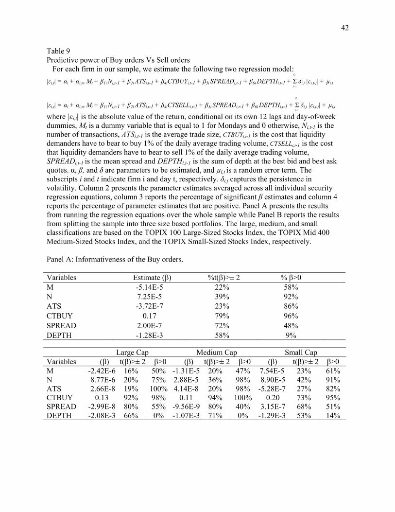
42

Table 9 Predictive power of Buy orders Vs Sell orders For each firm in our sample, we estimate the following two regression model: 12 |εi,t| = αi + αi,m Mt + β1i Ni,t-1 + β2i ATSi,t-1 + β4iCTBUYi,t-1 + β5i SPREADi,t-1 + β6i DEPTHi,t-1 + Σ δi,j |εi,t-j| + µi,t J=1 12 |εi,t| = αi + αi,m Mt + β1i Ni,t-1 + β2i ATSi,t-1 + β4iCTSELLi,t-1 + β5i SPREADi,t-1 + β6i DEPTHi,t-1 + Σ δi,j |εi,t-j| + µi,t J=1 where |εi,t| is the absolute value of the return, conditional on its own 12 lags and day-of-week dummies, Mt is a dummy variable that is equal to 1 for Mondays and 0 otherwise, Ni,t-1 is the number of transactions, ATSi,t-1 is the average trade size, CTBUYi,t-1 is the cost that liquidity demanders have to bear to buy 1% of the daily average trading volume, CTSELLi,t-1 is the cost that liquidity demanders have to bear to sell 1% of the daily average trading volume, SPREADi,t-1 is the mean spread and DEPTHi,t-1 is the sum of depth at the best bid and best ask quotes. α, β, and δ are parameters to be estimated, and µi,t is a random error term. The subscripts i and t indicate firm i and day t, respectively. δi,j captures the persistence in volatility. Column 2 presents the parameter estimates averaged across all individual security regression equations, column 3 reports the percentage of significant β estimates and column 4 reports the percentage of parameter estimates that are positive. Panel A presents the results from running the regression equations over the whole sample while Panel B reports the results from splitting the sample into three size based portfolios. The large, medium, and small classifications are based on the TOPIX 100 Large-Sized Stocks Index, the TOPIX Mid 400 Medium-Sized Stocks Index, and the TOPIX Small-Sized Stocks Index, respectively. Panel A: Informativeness of the Buy orders. Variables Estimate (β) %t(β)>± 2 % β>0 M -5.14E-5 22% 58% N 7.25E-5 39% 92% ATS -3.72E-7 23% 86% CTBUY 0.17 79% 96% SPREAD 2.00E-7 72% 48% DEPTH -1.28E-3 58% 9%

Large Cap Medium Cap Small Cap Variables (β) t(β)>± 2 β>0 (β) t(β)>± 2 β>0 (β) t(β)>± 2 β>0 M -2.42E-6 16% 50% -1.31E-5 20% 47% 7.54E-5 23% 61% N 8.77E-6 20% 75% 2.88E-5 36% 98% 8.90E-5 42% 91% ATS 2.66E-8 19% 100% 4.14E-8 20% 98% -5.28E-7 27% 82% CTBUY 0.13 92% 98% 0.11 94% 100% 0.20 73% 95% SPREAD -2.99E-8 80% 55% -9.56E-9 80% 40% 3.15E-7 68% 51% DEPTH -2.08E-3 66% 0% -1.07E-3 71% 0% -1.29E-3 53% 14%

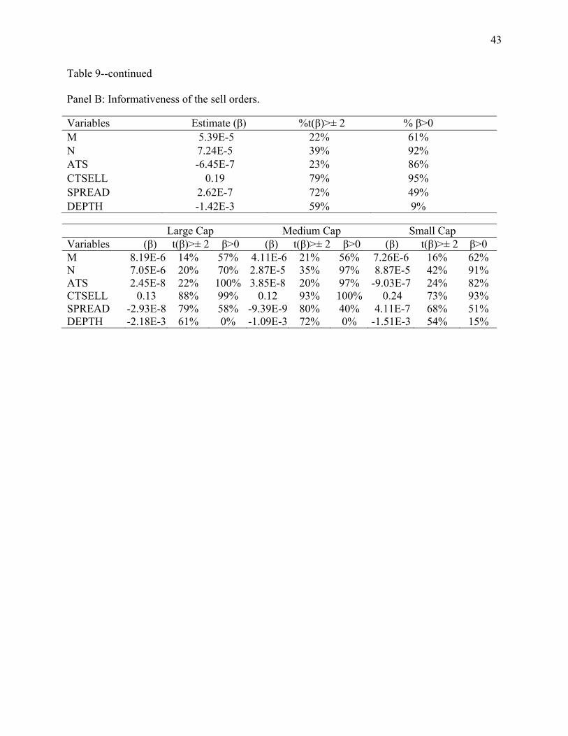
43

Table 9--continued Panel B: Informativeness of the sell orders. Variables Estimate (β) %t(β)>± 2 % β>0 M 5.39E-5 22% 61% N 7.24E-5 39% 92% ATS -6.45E-7 23% 86% CTSELL 0.19 79% 95% SPREAD 2.62E-7 72% 49% DEPTH -1.42E-3 59% 9%

Large Cap Medium Cap Small Cap Variables (β) t(β)>± 2 β>0 (β) t(β)>± 2 β>0 (β) t(β)>± 2 β>0 M 8.19E-6 14% 57% 4.11E-6 21% 56% 7.26E-6 16% 62% N 7.05E-6 20% 70% 2.87E-5 35% 97% 8.87E-5 42% 91% ATS 2.45E-8 22% 100% 3.85E-8 20% 97% -9.03E-7 24% 82% CTSELL 0.13 88% 99% 0.12 93% 100% 0.24 73% 93% SPREAD -2.93E-8 79% 58% -9.39E-9 80% 40% 4.11E-7 68% 51% DEPTH -2.18E-3 61% 0% -1.09E-3 72% 0% -1.51E-3 54% 15%

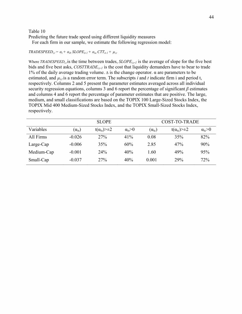
44

Table 10 Predicting the future trade speed using different liquidity measures For each firm in our sample, we estimate the following regression model: TRADESPEEDi,t = αi + αib SLOPEit-1 + αia CTTit-1 + µi,t Where TRADESPEEDi,t is the time between trades, SLOPEi,t-1 is the average of slope for the five best bids and five best asks, COSTTRADEi,t-1 is the cost that liquidity demanders have to bear to trade 1% of the daily average trading volume. is the change operator. α are parameters to be estimated, and µi,t is a random error term. The subscripts i and t indicate firm i and period t, respectively. Columns 2 and 5 present the parameter estimates averaged across all individual security regression equations, columns 3 and 6 report the percentage of significant β estimates and columns 4 and 6 report the percentage of parameter estimates that are positive. The large, medium, and small classifications are based on the TOPIX 100 Large-Sized Stocks Index, the TOPIX Mid 400 Medium-Sized Stocks Index, and the TOPIX Small-Sized Stocks Index, respectively.

SLOPE COST-TO-TRADE

Variables (αis) t(αis)>±2 αis>0 (αic) t(αic)>±2 αic>0

All Firms -0.026 27% 41% 0.08 35% 82%

Large-Cap -0.006 35% 60% 2.85 47% 90%

Medium-Cap -0.001 24% 40% 1.60 49% 95%

Small-Cap -0.037 27% 40% 0.001 29% 72%