Informed Options Trading on the Implied Volatility Surface:

A Cross-sectional Approach

Haehean Parka Baeho Kimb Dahae Kim0

Abstract

This paper investigates the cross-sectional implication of informed options trading across different

strikes and maturities. We adopt well-known option-implied volatility measures showing stock

return predictability to explore the term-structure perspective of the one-way information

transmission from options to stock markets. Using equity options data for U.S. listed stocks

covering 2000 to 2013, we find that the shape of the long-term implied volatility curve exhibits

extra predictive power for subsequent month stock returns even after orthogonalizing the short-

term components and existing predictors based on stock characteristics. Our finding indicates that

the inter-market information asymmetry rapidly disappears prior to the expiration of long-term

option contracts.

Key words: Implied volatility surface; Equity options; Stock return; Predictability; Informed

options trading;

JEL classification: G12; G13; G14

a Southwestern University of Finance and Economics (SWUFE), 55 Guanghuacun St, Chengdu, Sichuan 610074,

China; hhpark@swufe.edu.cn.

b Corresponding author: Korea University Business School, Anam-dong, Sungbuk-Gu, Seoul 136-701, Republic of

Korea; baehokim@korea.ac.kr; phone +82-2-3290-2626; fax +82-2-922-7220; http://biz.korea.ac.kr/~baehokim.

0 Department of Finance, Sungkyunkwan University, Seoul, Republic of Korea; dahea86@gmail.com; Phone

82+02+760+0951;

1

1 Introduction

The widespread use of various financial instruments across different maturities enables investors

to construct profitable strategies, as the instruments shed light on the market’s expectations for

future economic states and market conditions over different investment horizons. For example, it

is widely accepted that the shape of a yield curve extracted from short- and long-term bond prices

integrates the market’s anticipation of future interest rates and economic growth across time; see

Harvey (1988), Harvey (1991), Fama and French (1993) and Boudoukh and Richardson (1993)

among many others. Hendrik and Bessembinder (1995) examine the term structure perspective of

the futures market and find that mean reversion in asset prices occurs as an equilibrium

phenomenon in the futures markets. Han and Zhou (2011) examine the term structure of single-

name CDS spreads and show its negatively predictive power for future stock returns. Research on

the market volatility term structure has intensified as well. Merton (1973) claims in his

Intertemporal Capital Asset Pricing Model (ICAPM) that changes in the volatility term structure

should be priced in the cross-section of risky asset returns. Campbell and Viceira (2005) further

generalize the relevance of risk horizon effects on asset allocation by exploring the term-structure

of the risk–return tradeoff.

In this study, we consider the term structure of the option-implied volatility curve across

different strikes and maturities, as it reflects expected trends in the realized volatility of different

horizons in a forward-looking manner. An option-implied volatility surface is a function of both

moneyness and time-to-maturity. Thus, the time-varying implied volatility curve and term

structure are reflective of fluctuations in expectations of the risk-neutral distribution of underlying

asset returns based on the dynamics of the investment opportunity set in the market. Both

academics and practitioners have a long-standing interest in the options market, as it provides

informed investors with opportunities to capitalize on their information advantage. For example,

Jin, Livnat, and Zhang (2012) find that options traders are better able to process less-anticipated

information than are equity traders by analyzing the shape of implied volatility curves. Although

a considerable literature has grown around the theme of informed trading in the options market,

few studies have investigated stock return predictability in terms of the moneyness and maturity

2

dimensions at the same time. This paper fills this gap by examining the time-varying term structure

of option-implied volatility curves.

For the moneyness dimension, Xing, Zhang, and Zhao (2010) propose an implied volatility

smirk (IV smirk) measure by showing its significant predictability for the cross-section of future

equity returns. Jin, Livnat, and Zhang (2012) find that options traders are better able to process

less-anticipated information than are equity traders by analyzing the slope of option-implied

volatility curves. Using the spread between the ATM call and put option-implied volatilities (IV

spread) as a proxy of the average size of the jump in stock price dynamics, Yan (2011) find a

negative predictive relationship between IV spread and future stock returns. Constructing an

implied volatility convexity (IV convexity) measure, Park, Kim and Shim (2016) find that their

proposed IV convexity shows a cross-sectional predictive power for future stock returns in the

subsequent month, even after the slope of the implied volatility curve is taken out.

Remarkably, most studies examining the implied volatility curve use short-term (usually

one-month) maturity options when calculating the implied volatility shape measures. By contrast,

this paper contributes to the literature by studying the informational content of the term structure

of the options-implied volatility curve at the firm level and examining its predictive power for the

cross-section of stock returns. In the broader context, however, a considerable body of literature

has grown up around the theme of asset return predictability from the term structure perspective.

For instance, Xie (2014) finds that stocks with high sensitivities to changes in the VIX slope exhibit

high returns on average, as a downward sloping VIX term structure anticipates a potential long

disaster. Vasquez (2015) reports that the slope of the implied volatility term structure is positively

related to future option returns. Furthermore, Jones and Wang (2012) examine the relationship

between the slope of the implied volatility term structure and future option returns and find that

implied volatility slopes are positively correlated with the future returns on short-term straddles

while no clear relationship is observed for the returns on longer-term straddles. Andries, Eisenbach,

Schmalz and Wang (2015) investigate the price per unit of volatility risk at varying maturities and

find that the price per unit of volatility risk parameters are negative and decrease in absolute value

with maturity. Their finding is inconsistent with the standard asset pricing assumption of constant

risk aversion across maturities but confirms the horizon-dependent risk aversion asset pricing

3

modeling approach. Using index option data, Andries, Eisenbach and Schmalz (2014) show that

the preferences of horizon-dependent risk aversion generate a decreasing term structure of risk

premia if and only if volatility is stochastic; they argue that the price of risk depends on the horizon

and the horizon-dependent risk appetite has a meaningful impact on asset pricing. Vogt (2014)

investigates the term structures of variance risk premium using the VIX index and finds that the

term structure of the variance risk premium is dominated by compensation for bearing short-run

variance risk. Johnson (2016) finds that the changes in the shape of the VIX term structure contain

information about time-varying variance risk premia rather than expected changes in the VIX, thus

rejecting the expectation hypothesis. We notice that most studies focus on the term structure of the

option- implied volatility on the at-the-money level and overlook the importance of the changes in

the shape of the implied volatility curve across different strike prices over time.

To the best of our knowledge, this study is the first to consider both the implied volatility

smile (smirk) and its term structure at the same time in the context of informed options trading

relative to equity trading. By adopting well-known option-implied volatility measures showing

stock return predictability, we explore the term-structure perspective of informed trading in the

options market. Whereas prior studies typically measure the slope of the implied volatility term

structure, we devise our measure by orthogonalizing short-term volatility from long-term volatility

movements. Unlike with the simple difference between long- and short-term components, our

proposed measure corrects for the fact that implied volatility curves tend to flatten as time-to-

maturity increases, ceteris paribus. It is widely observed that the volatility term structure is

differently curved across different moneyness points, as the volatility implied by short-dated

option prices changes faster than that implied by longer-term options, partly because of the mean-

reversion effect of the (potentially) stochastic volatility process.

Using equity options data for U.S. listed stocks covering 2000 to 2013, we find that the

shape of the long-term implied volatility curve shows extra predictive power for subsequent

months’ stock returns even after we take out their short-term components and existing predictors

based on stock characteristics. Specifically, the average return differential between the lowest and

highest orthogonalized implied volatility spread/smirk/convexity quintile portfolios exceeds a

range of 0.38% to 0.52% per month, which is both economically and statistically significant on a

4

risk-adjusted basis. Our finding indicates that the transmission of long-term private information

from the options market to the stock market occurs prior to the expiration of the options. Thus,

informed long-term options trading contributes to the short-term price discovery process, as the

equity market updates its valuation by digesting the information prevailing in the options market

prior to the expiration of the options. Our findings are robust across different term spreads and

various holding periods.

The rest of this paper is organized as follows. Section 2 describes our dataset and variable

definitions. Section 3 presents the empirical results for the main hypotheses. Section 4 provides

additional tests as robustness checks, and Section 5 concludes the paper.

2 Data and Construction of Variables

This section describes our dataset and the methodology used to calculate the term structure of

implied volatility spread orthogonalized by one-month implied volatility spread (Ortho Spread,

hereafter), the term structure of implied volatility smirk orthogonalized by one-month implied

volatility smirk (Ortho Smirk, hereafter), and the term structure of implied volatility convexity

orthogonalized by one-month implied volatility convexity (Ortho Convexity, hereafter). We then

test whether each of Ortho Spread, Ortho Smirk, and Ortho Convexity exhibits significant

predictive power for future stock returns even if these variables are orthogonalized by one-month

component from long-term, six-month, implied volatility spread (smirk, convexity).

2.1 Data Description

The data for our study come from three primary sources: the OptionMetrics, the Center for

Research in Securities Prices (CRSP), and Compustat. We begin our sample selection with the U.S.

equity and index option data from the OptionMetrics database covering January 2000 to July 2013.

As the raw data include individual equity options in the American style, the OptionMetrics

applies the binomial tree model of Cox, Ross, and Rubinstein (1979) to estimate the option-implied

volatility curve to account for the possibility of an early exercise with discrete dividend payments

over the lives of the options, and OptionMetrics computes the interpolated implied volatility

5

surface separately for puts and calls using a kernel smoothing algorithm employing options with

various strikes and maturities.

Employing a kernel smoothing technique, OptionMetrics offers a volatility surface dataset

containing the implied volatilities for a list of standardized options for constant maturities and

deltas. Specifically, we obtain the fitted implied volatilities on a grid of fixed time-to-maturities

(30 days, 60 days, 90 days, 180 days, and 360 days) and option deltas (0.2, 0.25, …, 0.8 for calls

and -0.8, -0.75, … , -0.2 for puts), respectively. In our empirical analyses, we then select the

options with 180-day time-to-maturity as a representative value for long-term options and 30-day

time-to-maturity as a representative value for short-term options to estimate Ortho Spread, Ortho

Smirk, and Ortho Convexity.

[Insert Table 1 about here.]

Panel A of Table 1 shows the summary statistics of the fitted implied volatility and fixed

deltas of the individual equity options with one-month (30 days), two-month (60 days), three-

month (91 days), and six-month (182 days) time-to-maturity chosen at the end of each month. We

can clearly observe a positive convexity in the option-implied volatility curve as a function of the

option’s delta, in that the implied volatilities from in-the-money (ITM; calls for delta in the range

of 0.55 to 0.80, puts for delta of -0.80 to -0.55) options and OTM (calls for delta of 0.20 to 0.45,

puts for delta of -0.45 to -0.20) options are greater on average than those near the ATM options

(calls for delta of 0.50, puts for delta of -0.50). Panel B of Table 1 presents the unique number of

firms by industry each year. Each firm is placed into one of the 12 Fama–French industry (FF1-

12) classifications based on the SIC code. There are 2,900 unique firms in 2000, rising to 4,159 in

2013. We obtain daily and monthly individual common stock (shrcd of 10 or 11) returns from the

Center for Research in Security Prices (CRSP) for stocks traded on the NYSE (exchcd=1), Amex

(exchcd=2), and NASDAQ (exchcd=3). Accounting data are obtained from Compustat. We obtain

both daily and monthly data for each factor from Kenneth R. French’s website

(http://mba.tuck.dartmouth.edu/pages/faculty/ken.french/data_library.html).

6

2.2. Variable Construction

The option-implied volatility curve is a function not only of moneyness but also of time-to

expiration. The term structure of the option-implied volatility curve may convey useful

information about investors’ horizon-dependent risk aversion or expectations for asset prices.

Moreover, the slope of the option-implied volatility curve term structure contributes to the

prediction of realized higher moments of underlying assets over the life of options and delivers

crucial information about future stock prices. In contrast to the previous studies, which look into

the term structure of the options implied volatility at the ATM level and overlook the importance

of the change in implied volatility across moneyness over the life of options, we consider implied

volatility curve in an aspect of both the term structure and the moneyness characteristics and study

the informational content of the term structure of options implied volatility curve at the individual

firm level and examine their predictive power for the cross-section of stock returns.

To verify the relationship between the term structure of the option-implied volatility curve

and the expected equity return, we introduce three measures for the term-structure perspective of

the implied volatility curve—Ortho Spread, Ortho Smirk, and Ortho Convexity—representing the

change in the implied volatility curve over the life of options. We first calculate variables related

to daily long- and short-term option-implied volatility curves following Yan (2011), Xing, Zhang

and Zhao (2010), and Park, Kim and Shim (2016). We chose options with six-month time-to-

maturity as a benchmark of long-term options and options with one-month time-to-maturity as a

benchmark of short-term options. These variables are defined as follows:

𝑆𝑝𝑟𝑒𝑎𝑑6𝑚 (𝑜𝑟 1𝑚) = IVput,6𝑚 (𝑜𝑟 1𝑚)(∆= −0.5) − IVcall,6𝑚 (𝑜𝑟 1𝑚)(∆= 0.5) (1)

𝑆𝑚𝑖𝑟𝑘6𝑚 (𝑜𝑟 1𝑚) = IVput,6𝑚 (𝑜𝑟 1𝑚)(∆= −0.2) − IVcall,6𝑚 (𝑜𝑟 1𝑚)(∆= 0.5) (2)

𝐶𝑜𝑛𝑣𝑒𝑥𝑖𝑡𝑦6𝑚 (𝑜𝑟 1𝑚) = IVput,6𝑚 (𝑜𝑟 1𝑚)(∆= −0.2) + IVput,6𝑚 (𝑜𝑟 1𝑚)(∆= −0.8) − 2 ×

IVcall,6𝑚 (𝑜𝑟 1𝑚)(∆= 0.5) (3)

where 𝐼𝑉𝑝𝑢𝑡(Δ) and 𝐼𝑉𝑐𝑎𝑙𝑙(Δ) refer to the fitted put and call option-implied volatilities with six

months (or one month) to expiration, and Δ is the options’ delta. Note that using an option’s delta

is common industry practice to measure moneyness, as it is sensitive to the option’s intrinsic and

time values at the same time. As proposed by Yan (2011), 𝑆𝑝𝑟𝑒𝑎𝑑6𝑚 (𝑜𝑟 1𝑚) is the slope of the

7

option-implied volatility curve that captures the effect of the average jump size (𝜇𝐽) in the SVJ

model framework; this measure contains information about the ex-ante 3rd moment in the option-

implied distribution of the stock returns over the life (six months or one month) of the options.

Following Xing et al. (2010), 𝑆𝑚𝑖𝑟𝑘6𝑚 (𝑜𝑟 1𝑚) is defined as the OTM (∆= −0.2) put implied

volatility less the ATM (∆= 0.5) call implied volatility. This measure contains information on

both the 3rd and 4th moments of the stock return in a mixed manner. Next, 𝐶𝑜𝑛𝑣𝑒𝑥𝑖𝑡𝑦6𝑚 (𝑜𝑟 1𝑚),

proposed by Park et al. (2016), is defined as the average of the sum of OTM and ITM put implied

volatilities minus double the ATM call implied volatility. 𝐶𝑜𝑛𝑣𝑒𝑥𝑖𝑡𝑦6𝑚 (𝑜𝑟 1𝑚) is a simple proxy

for the volatility of stochastic volatility (𝜎𝑣) and jump size volatility (𝜎𝐽) in SV and SVJ framework.

The authors argue that the information delivered by 𝐶𝑜𝑛𝑣𝑒𝑥𝑖𝑡𝑦6𝑚 (𝑜𝑟 1𝑚) incorporates the

market’s expectation of the future tail-risk aversion of the underlying stock return over the lifetime

of the option.

The previous studies employ all the variables above based on one-month options and thus

capture the effect of the one-month implied volatility curve alone, not the effect of the longer-term

(six-month) implied volatility curve, on the implied distribution of the underlying stock returns.

Viewed in this vein, the main research question in this paper is whether the long-term implied

volatility spread still carries extra predictability for future stock returns even after we remove the

short-term component from it.

OptionMetrics provides the fitted implied volatilities on a grid of fixed time-to-maturities

of 30 days, 60 days, 90 days, 180 days, and 360 days. We consider 180-day (six-month) options

as long-term implied volatility and 30-day (one-month) options as short-term implied volatility.

Alternative definitions for the term structure of implied volatility curve-related variables across

different time-to-maturities do not materially change our main results.

Using daily 𝑆𝑝𝑟𝑒𝑎𝑑6𝑚 ( 𝑆𝑚𝑖𝑟𝑘6𝑚 , 𝐶𝑜𝑛𝑣𝑒𝑥𝑖𝑡𝑦6𝑚 ) and 𝑆𝑝𝑟𝑒𝑎𝑑1𝑚 ( 𝑆𝑚𝑖𝑟𝑘1𝑚 ,

𝐶𝑜𝑛𝑣𝑒𝑥𝑖𝑡𝑦1𝑚 ), we conduct time series regressions for each month to decompose 𝑆𝑝𝑟𝑒𝑎𝑑6𝑚

(𝑆𝑚𝑖𝑟𝑘6𝑚 , 𝐶𝑜𝑛𝑣𝑒𝑥𝑖𝑡𝑦6𝑚 ) into the predictive component and orthogonalized component by

𝑆𝑝𝑟𝑒𝑎𝑑1𝑚 (𝑆𝑚𝑖𝑟𝑘1𝑚, 𝐶𝑜𝑛𝑣𝑒𝑥𝑖𝑡𝑦1𝑚) to disentangle the slope of the term structure of the implied

volatility curve from the information on the long-term implied volatility curve as follows:

8

𝑆𝑝𝑟𝑒𝑎𝑑6𝑚,𝑖,𝑡−30~𝑡 = 𝛼𝑖 + 𝑏𝑖𝑆𝑝𝑟𝑒𝑎𝑑1𝑚,𝑖,𝑡−30~𝑡 + 𝜀𝑖,𝑡 (4)

𝑆𝑚𝑖𝑟𝑘6𝑚,𝑖,𝑡−30~𝑡 = 𝛼𝑖 + 𝑏𝑖𝑆𝑚𝑖𝑟𝑘1𝑚,𝑖,𝑡−30~𝑡 + 𝜀𝑖,𝑡 (5)

𝐶𝑜𝑛𝑣𝑒𝑥𝑖𝑡𝑦6𝑚,𝑖,𝑡−30~𝑡 = 𝛼𝑖 + 𝑏𝑖𝐶𝑜𝑛𝑣𝑒𝑥𝑖𝑡𝑦1𝑚,𝑖,𝑡−30~𝑡 + 𝜀𝑖,𝑡 (6)

The residual terms at the end of each month are defined as 𝑂𝑟𝑡ℎ𝑜 𝑆𝑝𝑟𝑒𝑎𝑑 6𝑚,1𝑚 ,

𝑂𝑟𝑡ℎ𝑜 𝑆𝑚𝑖𝑟𝑘6𝑚,1𝑚 , and 𝑂𝑟𝑡ℎ𝑜 𝐶𝑜𝑛𝑣𝑒𝑥𝑖𝑡𝑦6𝑚,1𝑚 , respectively. To reduce the impact of

infrequent trading on estimates, a minimum of 10 trading days in a month is required.

𝑂𝑟𝑡ℎ𝑜 𝑆𝑝𝑟𝑒𝑎𝑑 6𝑚,1𝑚 (𝑂𝑟𝑡ℎ𝑜 𝑆𝑚𝑖𝑟𝑘6𝑚,1𝑚, 𝑂𝑟𝑡ℎ𝑜 𝐶𝑜𝑛𝑣𝑒𝑥𝑖𝑡𝑦 6𝑚,1𝑚) is the term structure of the

option-implied volatility curve orthogonalized by the one-month option-implied volatility curve.

This variable contains the information about how Spread (Smirk, Convexity) will fluctuate from

long- to short-term options’ time intervals and how it will change over the life of the options. This

decomposition enables us to investigate whether the term structure of implied volatility curve-

related variables (from six- to one-month) and implied volatility curve-related variables (one-

month) has a distinct impact on a cross-section of future stock returns, which determines whether

𝑂𝑟𝑡ℎ𝑜 𝑆𝑝𝑟𝑒𝑎𝑑 6𝑚,1𝑚 ( 𝑂𝑟𝑡ℎ𝑜 𝑆𝑚𝑖𝑟𝑘6𝑚,1𝑚, 𝑂𝑟𝑡ℎ𝑜 𝐶𝑜𝑛𝑣𝑒𝑥𝑖𝑡𝑦 6𝑚,1𝑚) carries extra predictive

power for future stock returns, controlling for the return predictability of 𝑆𝑝𝑟𝑒𝑎𝑑1𝑚 (𝑆𝑚𝑖𝑟𝑘1𝑚,

𝐶𝑜𝑛𝑣𝑒𝑥𝑖𝑡𝑦1𝑚) of stock return distribution, as identified by Yan (2011), Xing et al. (2010), and

Part et al. (2016).

We define a firm’s size (Size) as the natural logarithm of market capitalization

(prc×shrout×1000), which is computed at the end of each month using CRSP data. When

computing book-to-market ratio (BTM), we match the yearly book value of equity, or BE (book

value of common equity [CEQ] plus deferred taxes and investment tax credit [txditc]) for all fiscal

years ending in June at year t to returns starting in July of year t-1, and divide this BE by the market

capitalization at month t-1. Hence, the book-to-market ratio is computed on a monthly basis.

Market betas (β) are estimated with rolling regressions using the previous 36 monthly returns

available up to month t-1 (a minimum of 12 months) given by

(Ri − Rf)𝑘 = αi

+ β i

(MKT − Rf)𝑘 + εi,k

, (7)

9

where t − 36 ≤ k ≤ t − 1 on a monthly basis. Following Jegadeesh and Titman (1993), we

compute momentum (MOM) using cumulative returns over the past six months, skipping one

month between the portfolio formation period and the computation period to exclude the reversal

effect. Momentum is also rebalanced every month and assumed to be held for the next one month.

Short-term reversal (REV) is estimated based on the past one-month return, as in Jegadeesh (1990)

and Lehmann (1990). Motivated by Amihud (2002) and Hasbrouck(2009), we define illiquidity

(ILLIQ) as the average of the absolute value of the stock return divided by the trading volume of

the stock in thousand USD using the past one-year’s daily data up to month t.

Adopting Ang, Hodrick, Xing, and Zhang (2006), we compute idiosyncratic volatility

using daily returns. The daily excess returns of individual stocks over the last 30 days are regressed

on Fama and French’s (1993, 1996) three factors daily and momentum factors monthly, where the

regression specification is given by

(Ri − Rf)𝑘 = αi

+ β1i

(MKT − Rf)k + β2i

SMBk + β3i

HMLk + β4i

WMLk + εk

, (8)

where t − 30 ≤ k ≤ t − 1 on a daily basis. Idiosyncratic volatility is computed as the standard

deviation of the regression residuals in every month. To reduce the impact of infrequent trading

on idiosyncratic volatility estimates, a minimum of 15 trading days in a month for which CRSP

reports both a daily return and non-zero trading volume is required.

We estimate systematic volatility using the method suggested by Duan and Wei (2009):

𝑣𝑠𝑦𝑠2 = 𝛽2𝑣M

2 /𝑣2 for every month. We also compute idiosyncratic implied variance as 𝑣𝑖𝑑𝑖𝑜2 =

𝑣2 − 𝛽2𝑣𝑀2 on a monthly basis, where vM is the implied volatility of the S&P500 index option,

following Dennis, Mayhew, and Stivers (2006).

[Insert Table 2 about here.]

Panel A of Table 2 shows the descriptive statistics of 𝑆𝑝𝑟𝑒𝑎𝑑6𝑚 ( 𝑆𝑚𝑖𝑟𝑘6𝑚 ,

𝐶𝑜𝑛𝑣𝑒𝑥𝑖𝑡𝑦6𝑚 ), 𝑆𝑝𝑟𝑒𝑎𝑑1𝑚 ( 𝑆𝑚𝑖𝑟𝑘1𝑚 , 𝐶𝑜𝑛𝑣𝑒𝑥𝑖𝑡𝑦1𝑚 ), and 𝑂𝑟𝑡ℎ𝑜 𝑆𝑝𝑟𝑒𝑎𝑑 6𝑚,1𝑚

(𝑂𝑟𝑡ℎ𝑜 𝑆𝑚𝑖𝑟𝑘 6𝑚,1𝑚 , 𝑂𝑟𝑡ℎ𝑜 𝐶𝑜𝑛𝑣𝑒𝑥𝑖𝑡𝑦 6𝑚,1𝑚). The average values for each variable are the

following: 𝑆𝑝𝑟𝑒𝑎𝑑1𝑚 ( 𝑆𝑝𝑟𝑒𝑎𝑑6𝑚) has 0.009(0.011), 𝑆𝑚𝑖𝑟𝑘1𝑚 ( 𝑆𝑚𝑖𝑟𝑘6𝑚 ) 0.069 (0.058) and

10

𝐶𝑜𝑛𝑣𝑒𝑥𝑖𝑡𝑦1𝑚(𝐶𝑜𝑛𝑣𝑒𝑥𝑖𝑡𝑦1𝑚) 0.095 (0.063). The standard deviation of 𝑆𝑝𝑟𝑒𝑎𝑑1𝑚 (𝑆𝑝𝑟𝑒𝑎𝑑6𝑚)

is 0.124 (0.086), that of 𝑆𝑚𝑖𝑟𝑘1𝑚 ( 𝑆𝑚𝑖𝑟𝑘6𝑚 ) is 0.142 (0.097), and that of

𝐶𝑜𝑛𝑣𝑒𝑥𝑖𝑡𝑦1𝑚 (𝐶𝑜𝑛𝑣𝑒𝑥𝑖𝑡𝑦1𝑚 ) is 0.279 (0.184). Concerning the end-of-month observations for

𝑂𝑟𝑡ℎ𝑜 𝑆𝑝𝑟𝑒𝑎𝑑 (𝑆𝑚𝑖𝑟𝑘, 𝐶𝑜𝑛𝑣𝑒𝑥𝑖𝑡𝑦)6𝑚,1𝑚 , the mean value of 𝑂𝑟𝑡ℎ𝑜 𝑆𝑝𝑟𝑒𝑎𝑑 6𝑚,1𝑚

(𝑂𝑟𝑡ℎ𝑜 𝑆𝑚𝑖𝑟𝑘6𝑚,1𝑚, 𝑂𝑟𝑡ℎ𝑜 𝐶𝑜𝑛𝑣𝑒𝑥𝑖𝑡𝑦 6𝑚,1𝑚) is 0 (0, -0.002), and the standard deviation of

𝑂𝑟𝑡ℎ𝑜 𝑆𝑝𝑟𝑒𝑎𝑑 6𝑚,1𝑚 (𝑂𝑟𝑡ℎ𝑜 𝑆𝑚𝑖𝑟𝑘 6𝑚,1𝑚, 𝑂𝑟𝑡ℎ𝑜 𝐶𝑜𝑛𝑣𝑒𝑥𝑖𝑡𝑦 6𝑚,1𝑚) is 0.041, (0.052, 0.086).

Panel B of Table 2 reports the descriptive statistics of the quintile portfolios sorted by each

firm characteristic variable (Size, BTM, Market β, MOM, REV, ILLIQ, and Coskew). The mean

and median of SIZE are 19.4607 and 19.3757, respectively, and BTM has a right-skewed

distribution, with a mean of 0.9186 and a median of 0.5472.

3 Empirical Analysis

3.1 Portfolio Analysis

The first empirical examination is whether 𝑂𝑟𝑡ℎ𝑜 𝑆𝑝𝑟𝑒𝑎𝑑 6𝑚,1𝑚 ( 𝑂𝑟𝑡ℎ𝑜 𝑆𝑚𝑖𝑟𝑘6𝑚,1𝑚,

𝑂𝑟𝑡ℎ𝑜 𝐶𝑜𝑛𝑣𝑒𝑥𝑖𝑡𝑦 6𝑚,1𝑚) can account for the cross-sectional variation of expected equity return.

To examine the relationship between 𝑂𝑟𝑡ℎ𝑜 𝑆𝑝𝑟𝑒𝑎𝑑 6𝑚,1𝑚 ( 𝑂𝑟𝑡ℎ𝑜 𝑆𝑚𝑖𝑟𝑘 6𝑚,1𝑚 ,

𝑂𝑟𝑡ℎ𝑜 𝐶𝑜𝑛𝑣𝑒𝑥𝑖𝑡𝑦 6𝑚,1𝑚) and future stock returns, we form five portfolios based on the value of

𝑂𝑟𝑡ℎ𝑜 𝑆𝑝𝑟𝑒𝑎𝑑 (𝑂𝑟𝑡ℎ𝑜 𝑆𝑚𝑖𝑟𝑘, 𝑂𝑟𝑡ℎ𝑜 𝐶𝑜𝑛𝑣𝑒𝑥𝑖𝑡𝑦)6𝑚,1𝑚 at the end of each month.

Quintile 1 is composed of stocks with the lowest 𝑂𝑟𝑡ℎ𝑜 𝑆𝑝𝑟𝑒𝑎𝑑 6𝑚,1𝑚

(𝑂𝑟𝑡ℎ𝑜 𝑆𝑚𝑖𝑟𝑘 6𝑚,1𝑚, 𝑂𝑟𝑡ℎ𝑜 𝐶𝑜𝑛𝑣𝑒𝑥𝑖𝑡𝑦 6𝑚,1𝑚) while Quintile 5 is composed of stocks with the

highest 𝑂𝑟𝑡ℎ𝑜 𝑆𝑝𝑟𝑒𝑎𝑑 6𝑚,1𝑚 (𝑂𝑟𝑡ℎ𝑜 𝑆𝑚𝑖𝑟𝑘6𝑚,1𝑚, 𝑂𝑟𝑡ℎ𝑜 𝐶𝑜𝑛𝑣𝑒𝑥𝑖𝑡𝑦 6𝑚,1𝑚). These portfolios

are equally weighted, rebalanced every month, and assumed to be held for the subsequent one-

month period.

[Insert Table 3 about here.]

Panel A presents the average number of firms, means, and standard deviations of the

𝑆𝑝𝑟𝑒𝑎𝑑6𝑚 , 𝑆𝑝𝑟𝑒𝑎𝑑1𝑚 , 𝑂𝑟𝑡ℎ𝑜 𝑆𝑝𝑟𝑒𝑎𝑑6𝑚,1𝑚 quintile portfolios and the average portfolio

monthly returns over the entire sample period. Examining the average returns across quintiles for

11

𝑆𝑝𝑟𝑒𝑎𝑑6𝑚 , the long-term implied volatility spread, reveals that stocks (Q1) with the lowest

𝑆𝑝𝑟𝑒𝑎𝑑6𝑚 provide 0.0149 of expected return per month on average and stocks (Q5) with the

highest 𝑆𝑝𝑟𝑒𝑎𝑑6𝑚 provide -0.0003, suggesting that the average returns on the quintile portfolios

sorted by 𝑆𝑝𝑟𝑒𝑎𝑑6𝑚 decrease monotonically in portfolio rank. In addition, the average monthly

return of the arbitrage portfolio buying the lowest 𝑆𝑝𝑟𝑒𝑎𝑑6𝑚 portfolio Q1 and selling highest

𝑆𝑝𝑟𝑒𝑎𝑑6𝑚 portfolio Q5 is significantly positive (0.0152, with t-statistics of 8.12).

Moreover, examining the portfolios sorted by 𝑆𝑝𝑟𝑒𝑎𝑑1𝑚 , the short-term implied

volatility spread, shows that their average returns decrease monotonically from 0.0143 for quintile

portfolio Q1 to 0.0012 for quintile portfolio Q5, and the average return difference between Q1 and

Q5 amounts to 0.013, with t-statistics of 7.44. These results confirm Yan’s (2011) empirical

finding that low 𝑆𝑝𝑟𝑒𝑎𝑑1𝑚 stocks outperform high 𝑆𝑝𝑟𝑒𝑎𝑑1𝑚 stocks. Overall, we find

significant evidence that stocks with lower quintiles have higher expected returns than do stocks

with higher quintiles for both long- and short-term implied volatility spreads. This result implies

that not only short-term implied volatility spread, 𝑆𝑝𝑟𝑒𝑎𝑑1𝑚, but also long-term implied volatility

spread, 𝑆𝑝𝑟𝑒𝑎𝑑6𝑚, has explanatory power in capturing stock return variation. As shown in Yan

(2011), there is a definitely negative predictive relationship between 𝑆𝑝𝑟𝑒𝑎𝑑1𝑚 and future stock

returns.

The main research question of this paper is whether the long-term implied volatility spread

still carries extra predictability for future stock returns even after we remove the short-term

component from it. To address it, we employ 𝑂𝑟𝑡ℎ𝑜 𝑆𝑝𝑟𝑒𝑎𝑑6𝑚,1𝑚 , the term structure of the

option-implied volatility curve orthogonalized by the one-month option-implied volatility curve,

and examine whether 𝑂𝑟𝑡ℎ𝑜 𝑆𝑝𝑟𝑒𝑎𝑑6𝑚,1𝑚 still carries extra predictability for future stock

returns beyond 𝑆𝑝𝑟𝑒𝑎𝑑1𝑚. The six right-hand columns are the results using portfolios sorted by

𝑂𝑟𝑡ℎ𝑜 𝑆𝑝𝑟𝑒𝑎𝑑6𝑚,1𝑚 . Although the arbitrage portfolio return is somewhat small (the value is

0.0044) compared to that of 𝑆𝑝𝑟𝑒𝑎𝑑6𝑚 (𝑆𝑝𝑟𝑒𝑎𝑑1𝑚), the average returns of the quintile portfolios

sorted by 𝑂𝑟𝑡ℎ𝑜 𝑆𝑝𝑟𝑒𝑎𝑑6𝑚,1𝑚 are decreasing in 𝑂𝑟𝑡ℎ𝑜 𝑆𝑝𝑟𝑒𝑎𝑑6𝑚,1𝑚 , and the returns of the

zero-investment portfolios (Q1–Q5) are all positive and statistically significant, confirming that

𝑂𝑟𝑡ℎ𝑜 𝑆𝑝𝑟𝑒𝑎𝑑6𝑚,1𝑚 , which contains information about how the ex-ante skewness of the

12

underlying stock return will fluctuate over the options’ lifetime, has additional explanatory power

for future stock returns beyond 𝑆𝑝𝑟𝑒𝑎𝑑1𝑚.

Panel B in Table 3 shows the average number of firms, means, and standard deviations of

the 𝑆𝑚𝑖𝑟𝑘6𝑚, 𝑆𝑚𝑖𝑟𝑘1𝑚, and 𝑂𝑟𝑡ℎ𝑜 𝑆𝑚𝑖𝑟𝑘6𝑚,1𝑚 quintile portfolios and the average portfolio

monthly returns over the entire sample period. Our empirical results show that the long-term smirk

measure, 𝑆𝑚𝑖𝑟𝑘6𝑚, generates a monotone decreasing pattern of the average quintile portfolio

returns, from 0.0147 per month for the bottom quintile to 0.0005 per month for the top quintile,

and that the realized returns of the arbitrage portfolio (Q1–Q5) has a positive value (0.0142) with

statistical significance (with a t-statistic of 6.92).

The average returns of the quintile portfolio sorted by short-term smirk measure,

𝑆𝑝𝑟𝑒𝑎𝑑1𝑚, also decline monotonically, going from quintile 1 to quintile 5, and the difference

between average returns on the portfolio with the highest and lowest 𝑆𝑝𝑟𝑒𝑎𝑑1𝑚 is around

0.0104, with a t-statistics of 5.16 per month. These results are consistent with Xing et al.’s (2010)

empirical findings that low 𝑆𝑚𝑖𝑟𝑘1𝑚 stocks outperform high 𝑆𝑚𝑖𝑟𝑘1𝑚 stocks. Overall, we find

significant evidence that both short-term implied volatility smirk, 𝑆𝑚𝑖𝑟𝑘1𝑚 , and long-term

implied volatility smirk, 𝑆𝑚𝑖𝑟𝑘6𝑚, have predictive power in forecasting future equity returns and

that, as shown in Xing et al. (2010), a definitely negative predictive relationship exists between

𝑆𝑚𝑖𝑟𝑘 and future stock returns.

In the case of 𝑂𝑟𝑡ℎ𝑜 𝑆𝑚𝑖𝑟𝑘6𝑚,1𝑚, the long-short zero investment portfolio of Q1–Q5 has

an average return of 0.0044 over the next month, with a t-statistics of 3.98. This long-short

portfolio return is smaller than that of 𝑆𝑝𝑟𝑒𝑎𝑑6𝑚 ( 𝑆𝑝𝑟𝑒𝑎𝑑1𝑚 ). 𝑂𝑟𝑡ℎ𝑜 𝑆𝑚𝑖𝑟𝑘6𝑚,1𝑚 is a

forward-looking measure capturing the change of higher moments in the implied distribution of

stock returns during the long- to the short-term options’ time intervals and how it changes over the

lifetime of the options. So these empirical results imply that 𝑂𝑟𝑡ℎ𝑜 𝑆𝑚𝑖𝑟𝑘6𝑚,1𝑚 delivers crucial

additional explanatory information for future stock returns beyond 𝑆𝑚𝑖𝑟𝑘1𝑚.

We next reconcile the relationship between the convexity of an option-implied volatility

curve, Convexity, and future stock returns. As Park et al. (2016) suggested, Convexity is a forward-

looking measure of excess tail-risk contribution to the perceived variance of underlying equity

13

returns. Panel C in Table 3 reports the average number of firms, means, and standard deviations

of the 𝐶𝑜𝑛𝑣𝑒𝑥𝑖𝑡𝑦6𝑚 , 𝐶𝑜𝑛𝑣𝑒𝑥𝑖𝑡𝑦1𝑚 , and 𝑂𝑟𝑡ℎ𝑜 𝐶𝑜𝑛𝑣𝑒𝑥𝑖𝑡𝑦6𝑚,1𝑚 quintile portfolios and the

average portfolio monthly returns over the entire sample. In the results for average returns across

Convexity quintile, the average returns of the quintile portfolios decline monotonically, and stocks

with the lowest 𝐶𝑜𝑛𝑣𝑒𝑥𝑖𝑡𝑦6𝑚 (𝐶𝑜𝑛𝑣𝑒𝑥𝑖𝑡𝑦1𝑚) provide 0.0149 (0.0136) of the expected average

returns, and stocks with the highest 𝐶𝑜𝑛𝑣𝑒𝑥𝑖𝑡𝑦6𝑚 (𝐶𝑜𝑛𝑣𝑒𝑥𝑖𝑡𝑦1𝑚) provide -0.0007 (0.018). In

addition, the average monthly return of the arbitrage portfolio buying the lowest

𝐶𝑜𝑛𝑣𝑒𝑥𝑖𝑡𝑦6𝑚 (𝐶𝑜𝑛𝑣𝑒𝑥𝑖𝑡𝑦1𝑚) portfolio Q1 and selling the highest 𝐶𝑜𝑛𝑣𝑒𝑥𝑖𝑡𝑦6𝑚 (𝐶𝑜𝑛𝑣𝑒𝑥𝑖𝑡𝑦1𝑚)

portfolio Q5 are significantly positive values. (0.0156, with a t-statistic of 8.56, for 𝐶𝑜𝑛𝑣𝑒𝑥𝑖𝑡𝑦6𝑚

and 0.0119, with a t-statistic of 7.07, for 𝐶𝑜𝑛𝑣𝑒𝑥𝑖𝑡𝑦1𝑚). This empirical result indicates that both

short-term implied volatility convexity, 𝐶𝑜𝑛𝑣𝑒𝑥𝑖𝑡𝑦1𝑚, and long-term implied volatility convexity,

𝐶𝑜𝑛𝑣𝑒𝑥𝑖𝑡𝑦6𝑚, have predictive ability in forecasting future equity returns, thus confirming Park et

al. (2016), who find that the average return differential between the lowest and highest convexity

quintile portfolios exceeds 1% per month, which is both economically and statistically significant

on a risk-adjusted basis.

Next, we decompose the information extracted from the six-month option-implied

volatility convexity into a predictive component and orthogonalized component by 𝐶𝑜𝑛𝑣𝑒𝑥𝑖𝑡𝑦1𝑚

and empirically verify that 𝑂𝑟𝑡ℎ𝑜 𝐶𝑜𝑛𝑣𝑒𝑥𝑖𝑡𝑦 6𝑚,1𝑚, has a significant predictive power for the

cross-section of future stock returns. The 𝐶𝑜𝑛𝑣𝑒𝑥𝑖𝑡𝑦1𝑚 measure proposed by Park et al. (2016)

captures the effect of the one-month implied volatility convexity, but not the effect of the longer-

term (six-month) implied volatility convexity, on the implied distribution of underlying stock

returns. The empirical evidence indicates that 𝑂𝑟𝑡ℎ𝑜 𝐶𝑜𝑛𝑣𝑒𝑥𝑖𝑡𝑦 6𝑚,1𝑚 carries additional

forecasting power for future stock returns even after we remove the information of short-term

component convexity from long-term convexity.

[Insert Figure 2 about here.]

The left-hand side of Panel A (Panel B, Panel C) in Figure 2 shows the monthly average

𝑂𝑟𝑡ℎ𝑜 𝑆𝑝𝑟𝑒𝑎𝑑 6𝑚,1𝑚 ( 𝑂𝑟𝑡ℎ𝑜 𝑆𝑚𝑖𝑟𝑘6𝑚,1𝑚, 𝑂𝑟𝑡ℎ𝑜 𝐶𝑜𝑛𝑣𝑒𝑥𝑖𝑡𝑦 6𝑚,1𝑚) value for each quintile

portfolio, while the right-hand side plots the monthly average return of the arbitrage portfolio

14

formed by taking a long position in the lowest quintile and a short position in the highest quintile

portfolios (Q1–Q5). The time-varying average monthly returns of the long-short portfolios based

on 𝑂𝑟𝑡ℎ𝑜 𝑆𝑝𝑟𝑒𝑎𝑑 6𝑚,1𝑚 ( 𝑂𝑟𝑡ℎ𝑜 𝑆𝑚𝑖𝑟𝑘6𝑚,1𝑚, 𝑂𝑟𝑡ℎ𝑜 𝐶𝑜𝑛𝑣𝑒𝑥𝑖𝑡𝑦 6𝑚,1𝑚) are mostly positive,

confirming the results reported in Table 3.

3.2 Time-series Analysis

In this section, we examine whether the existing risk factor models can explain the negative

relationship between 𝑂𝑟𝑡ℎ𝑜 𝑆𝑝𝑟𝑒𝑎𝑑6𝑚,1𝑚 (𝑂𝑟𝑡ℎ𝑜 𝑆𝑚𝑖𝑟𝑘6𝑚,1𝑚, 𝑂𝑟𝑡ℎ𝑜 𝐶𝑜𝑛𝑣𝑒𝑥𝑖𝑡𝑦6𝑚,1𝑚) and

stock return. If financial markets perfectly and completely function well and the mean-variance

efficiency of the market portfolio holds, market β is the only risk factor that can explain the cross-

sectional variations in expected returns, as argued in the capital asset pricing model (CAPM).

As investors cannot hold perfectly diversified portfolios, Fama and French (1996) find

that CAPM's measure of systematic risk is unreliable in practice and that firm size and book-to-

market ratio are more valid. They argue that the three-factor model in Fama and French (1993) can

capture the cross-sectional variations in equity returns better than the CAPM model. The Fama

and French (1993) model has three factors: (i) Rm − Rf (the excess return on the market), (ii)

SMB (the difference in returns between small stocks and big stocks), and (iii) HML (the difference

in returns between high book-to-market stocks and low book-to-market stocks).

To test whether the existing risk factor models can explain our result that

𝑂𝑟𝑡ℎ𝑜 𝑆𝑝𝑟𝑒𝑎𝑑6𝑚,1𝑚 (𝑂𝑟𝑡ℎ𝑜 𝑆𝑚𝑖𝑟𝑘6𝑚,1𝑚, 𝑂𝑟𝑡ℎ𝑜 𝐶𝑜𝑛𝑣𝑒𝑥𝑖𝑡𝑦6𝑚,1𝑚) provides a negative

prediction of the cross-section of future stock returns, we conduct a time-series test based on

CAPM and the Fama-French three factor model, respectively. In addition to CAPM and Fama-

French three factor model, we also conduct time-series analysis using an extended four-factor

model (Carhart, 1997) that includes a momentum factor (UMD) suggested by Jegadeesh and

Titman (1993; FF4).

[Insert Table 4 about here.]

Table 4 presents the coefficient of the CAPM, the three-factor model proposed in Fama

and French, and the four-factor model proposed in Carhart (1997), time-series regressions for

15

monthly excess returns on five portfolios sorted by 𝑂𝑟𝑡ℎ𝑜 𝑆𝑝𝑟𝑒𝑎𝑑6𝑚 ( 𝑂𝑟𝑡ℎ𝑜 𝑆𝑚𝑖𝑟𝑘1𝑚 ,

𝑂𝑟𝑡ℎ𝑜 𝐶𝑜𝑛𝑣𝑒𝑥𝑖𝑡𝑦6𝑚,1𝑚). The six left-hand columns are the results using a portfolio sorted by

𝑂𝑟𝑡ℎ𝑜 𝑆𝑝𝑟𝑒𝑎𝑑6𝑚,1𝑚 . The result shows that the estimated intercepts in the Q2 and Q3

𝑂𝑟𝑡ℎ𝑜 𝑆𝑝𝑟𝑒𝑎𝑑6𝑚,1𝑚 portfolio ( �̂�𝑄2, �̂�𝑄3 ) are statistically significant; we observe negative

patterns with respect to portfolios formed by 𝑂𝑟𝑡ℎ𝑜 𝑆𝑝𝑟𝑒𝑎𝑑6𝑚,1𝑚. A trading strategy of buying

the lowest and selling the highest (Q5) portfolio using 𝑂𝑟𝑡ℎ𝑜 𝑆𝑝𝑟𝑒𝑎𝑑6𝑚,1𝑚 ( �̂�𝑄5 − �̂�𝑄1 )

generates about 0.0037 alpha per month (t-statistic = 3.91) for CAPM, 0.0137 alpha per month (t-

statistic = 3.75) for FF3, and 0.0136 alpha per month (t-statistic =3.74) for FF4. Following Gibbons,

Ross, and Shanken (1989), we test the null hypothesis that all estimated intercepts are

simultaneously equal to zero (�̂�𝑄1 = ⋯ = �̂�𝑄5 = 0). The results show that this null hypothesis is

rejected with a p-value < 0.001 in the CAPM, FF3, and FF4 model specifications. The pattern of

alphas from the three different factor specifications implies that the abnormal returns of Q1-Q5

𝑂𝑟𝑡ℎ𝑜 𝑆𝑝𝑟𝑒𝑎𝑑6𝑚,1𝑚 portfolios are not specific to asset pricing models and confirms that the

widely accepted existing factors (Rm − 𝑅𝑓, SMB, HML, UMD) cannot fully capture and explain

the negative portfolio return patterns sorted by 𝑂𝑟𝑡ℎ𝑜 𝑆𝑝𝑟𝑒𝑎𝑑6𝑚,1𝑚. We may thus argue that the

existing systematic risk factors cannot capture the information of 𝑂𝑟𝑡ℎ𝑜 𝑆𝑝𝑟𝑒𝑎𝑑6𝑚,1𝑚. Therefore,

we argue that 𝑂𝑟𝑡ℎ𝑜 𝑆𝑝𝑟𝑒𝑎𝑑6𝑚,1𝑚 has additional explanatory power for capturing the cross-

sectional variations in equity returns that cannot be fully explained by existing models (CAPM,

FF3, and FF4).

When we conduct a time-series test using portfolios sorted by 𝑂𝑟𝑡ℎ𝑜 𝑆𝑚𝑖𝑟𝑘6𝑚,1𝑚 to see

whether the effect of 𝑂𝑟𝑡ℎ𝑜 𝑆𝑚𝑖𝑟𝑘6𝑚,1𝑚 can be explained by existing risk factors, the alphas of

the quintile port folios sorted by 𝑂𝑟𝑡ℎ𝑜 𝑆𝑚𝑖𝑟𝑘6𝑚,1𝑚 decline monotonically, from 0.0038

(0.0012, 0.0019) per month for the bot tom quintile to -0.0005 (-0.0032, -0.0025) per month for

the top quintile for the CAPM (FF3, FF4) model. The 𝑂𝑟𝑡ℎ𝑜 𝑆𝑚𝑖𝑟𝑘6𝑚,1𝑚 portfolio with

long stocks in the bottom 𝑂𝑟𝑡ℎ𝑜 𝑆𝑚𝑖𝑟𝑘6𝑚,1𝑚 quintile and short stocks in the top quintile has a

monthly alpha of 0.0043 (t-statistic = 3.62), 0.0044 (t-statistic = 3.91), and 0.0044 (t-statistic =

3.95) with respect to the CAPM, the Fama–French three-factor, and the Carhart four-factor model,

respectively. The joint tests from Gibbons, Ross, and Shanken (1989) examining whether the

model explains the average portfolio returns sorted by 𝑂𝑟𝑡ℎ𝑜 𝑆𝑚𝑖𝑟𝑘6𝑚,1𝑚 are strongly rejected

16

with a p-value < 0.001 for the CAPM, FF3, and FF4 models. This result implies that

𝑂𝑟𝑡ℎ𝑜 𝑆𝑚𝑖𝑟𝑘6𝑚,1𝑚 is not explained by existing systematic risk factors. Thus, we infer that it is

difficult to explain the decreasing pattern of portfolio returns shown in 𝑂𝑟𝑡ℎ𝑜 𝑆𝑚𝑖𝑟𝑘6𝑚,1𝑚 using

existing traditional risk-based factor models and that 𝑂𝑟𝑡ℎ𝑜 𝑆𝑚𝑖𝑟𝑘6𝑚,1𝑚 can capture the cross-

sectional variations in equity returns that cannot be fully explained by existing models (CAPM,

FF3, and FF4).

As shown in the six right-hand columns, similar economically and statistically significant

results are obtained for the monthly returns on 𝑂𝑟𝑡ℎ𝑜 𝐶𝑜𝑛𝑣𝑒𝑥𝑖𝑡𝑦6𝑚,1𝑚 portfolios. The alpha

differences between the lowest 𝑂𝑟𝑡ℎ𝑜 𝐶𝑜𝑛𝑣𝑒𝑥𝑖𝑡𝑦6𝑚,1𝑚 and highest 𝑂𝑟𝑡ℎ𝑜 𝐶𝑜𝑛𝑣𝑒𝑥𝑖𝑡𝑦6𝑚,1𝑚

portfolios are in the range of 0.0050 to 0.0052 per month, and are significant. For example, the

CAPM alpha of the Q1–Q5 𝑂𝑟𝑡ℎ𝑜 𝐶𝑜𝑛𝑣𝑒𝑥𝑖𝑡𝑦6𝑚,1𝑚 is 0.0050 per month with 4.14 t-statistics,

and the four-factor alpha is 0.0052 per month with 4.46 t-statistics.

3.3. Fama–Macbeth Regression

Having found the significance of the 𝑂𝑟𝑡ℎ𝑜 𝑆𝑝𝑟𝑒𝑎𝑑6𝑚,1𝑚 ( 𝑂𝑟𝑡ℎ𝑜 𝑆𝑚𝑖𝑟𝑘6𝑚,1𝑚 ,

𝑂𝑟𝑡ℎ𝑜 𝐶𝑜𝑛𝑣𝑒𝑥𝑖𝑡𝑦6𝑚,1𝑚) as a determinant of the expected equity returns at the portfolio level, we

turn to address additional aspect of 𝑂𝑟𝑡ℎ𝑜 𝑆𝑝𝑟𝑒𝑎𝑑6𝑚,1𝑚 ( 𝑂𝑟𝑡ℎ𝑜 𝑆𝑚𝑖𝑟𝑘6𝑚,1𝑚 ,

𝑂𝑟𝑡ℎ𝑜 𝐶𝑜𝑛𝑣𝑒𝑥𝑖𝑡𝑦6𝑚,1𝑚 ) measurements for robustness. We conduct a Fama–Macbeth (1973)

regression analysis at the firm level with various control variables to document the robustness of

the cross-sectional negative relationship between 𝑂𝑟𝑡ℎ𝑜 𝑆𝑝𝑟𝑒𝑎𝑑6𝑚,1𝑚 ( 𝑂𝑟𝑡ℎ𝑜 𝑆𝑚𝑖𝑟𝑘6𝑚,1𝑚 ,

𝑂𝑟𝑡ℎ𝑜 𝐶𝑜𝑛𝑣𝑒𝑥𝑖𝑡𝑦6𝑚,1𝑚) and the expected stock returns and investigate whether IV convexity has

sufficient explanatory power beyond others suggested in the literature. In a Fama–Macbeth

regression, the dependent variable is one-month ahead monthly returns.

We control for Market 𝛽 (estimated following Fama and French [1992]), log market

capitalization (ln_mv), book-to-market ratio (btm), momentum (MOM), reversal (REV), illiquidity

(ILLIQ), options volatility slope (IV spread and IV smirk), and idiosyncratic risk (idio_risk) as

common measures of risks that explain stock returns. We also include the measure of the option-

implied volatility-related variables, implied volatility level (IV level), systematic implied volatility

17

(𝑣𝑠𝑦𝑠2 ), and idiosyncratic implied variance (𝑣𝑖𝑑𝑖𝑜

2 ), as suggested by Duan and Wei (2009) and

Dennis, Mayhew, and Stivers (2006). We run the monthly cross-sectional regression of individual

stock returns of the subsequent month on 𝑆𝑝𝑟𝑒𝑎𝑑1𝑚 ( 𝑆𝑚𝑖𝑟𝑘1𝑚 , 𝐶𝑜𝑛𝑣𝑒𝑥𝑖𝑡𝑦1𝑚 ),

𝑂𝑟𝑡ℎ𝑜 𝑆𝑝𝑟𝑒𝑎𝑑6𝑚,1𝑚(𝑂𝑟𝑡ℎ𝑜 𝑆𝑚𝑖𝑟𝑘6𝑚,1𝑚, 𝑂𝑟𝑡ℎ𝑜 𝐶𝑜𝑛𝑣𝑒𝑥𝑖𝑡𝑦6𝑚,1𝑚) and other known measures

of risks presented above.

[Insert Table 5 about here.]

Panel A in Table 5 reports the time-series averages of the coefficients from the regressions

of expected stock returns on the 𝑆𝑝𝑟𝑒𝑎𝑑1𝑚, 𝑂𝑟𝑡ℎ𝑜 𝑆𝑝𝑟𝑒𝑎𝑑6𝑚,1𝑚, beta, size, book-to-market

ratio, momentum, short-term reversal, illiquidity, idiosyncratic risk, IV level, and 𝑣𝑠𝑦𝑠2 𝑣𝑖𝑑𝑖𝑜

2 with

the Newey–West adjusted t-statistics for the time-series average of coefficients with a lag of 3 over

the sample period of 2000 to 2013. The column of Model 1 shows that the coefficient on

𝑆𝑝𝑟𝑒𝑎𝑑1𝑚 is significantly negative, confirming Yan’s (2011) finding demonstrating the negative

predictive relationship between 𝑆𝑝𝑟𝑒𝑎𝑑1𝑚 and future stock returns. When we include both

𝑆𝑝𝑟𝑒𝑎𝑑1𝑚 and 𝑂𝑟𝑡ℎ𝑜 𝑆𝑝𝑟𝑒𝑎𝑑6𝑚,1𝑚 as shown in Model 2, the coefficients on

𝑂𝑟𝑡ℎ𝑜 𝑆𝑝𝑟𝑒𝑎𝑑6𝑚,1𝑚 are significantly negative, indicating that 𝑂𝑟𝑡ℎ𝑜 𝑆𝑝𝑟𝑒𝑎𝑑6𝑚,1𝑚 has

additional explanatory power for stock returns that 𝑆𝑝𝑟𝑒𝑎𝑑1𝑚 cannot fully capture. This result

suggests that not only 𝑆𝑝𝑟𝑒𝑎𝑑1𝑚 but 𝑂𝑟𝑡ℎ𝑜 𝑆𝑝𝑟𝑒𝑎𝑑6𝑚,1𝑚 exhibits significant predictive power

for stock returns, confirming the univariate sort ing results in Table 3. The column of Model 3

and 4 shows the Fama–Macbeth regression results using market β and other stock fundamentals

including firm-size (ln_mv), book-to-market ratio (btm), other systematic risks, MOM, REV, and

ILLIQ. These variables are widely accepted stock characteristics that can capture the cross-

sectional variation in stock returns. When the six control variables are included in the regression,

not only the coefficient on 𝑆𝑝𝑟𝑒𝑎𝑑1𝑚 but also that on 𝑂𝑟𝑡ℎ𝑜 𝑆𝑝𝑟𝑒𝑎𝑑6𝑚,1𝑚 has negative values

with negative significance. This result from cross-sectional regressions shows strong corroborating

evidence for an economically and statistically significant negative relationship between the degree

of 𝑂𝑟𝑡ℎ𝑜 𝑆𝑝𝑟𝑒𝑎𝑑6𝑚,1𝑚 and the expected stock returns.

Model 5 and Model 6 represent the Fama–Macbeth regression result using market β,

ln_mv, btm, MOM, REV, ILLIQ, and idiosyncratic risk. The estimated coefficient on idiosyncratic

18

risk suggested by Ang, Hodrick, Xing, and Zhang (2006) has a negative value and is significant.

If an ideal asset pricing model can fully captures the cross-sectional variation in stock return,

idiosyncratic risk should not be significantly priced. The relationship between idiosyncratic risk

and stock returns is inconclusive and a matter of controversy among researchers. Ang, Hodrick,

Xing, and Zhang (2006) show that stocks with low idiosyncratic risk earn higher average returns

compared to high idiosyncratic risk portfolios and that the arbitrage portfolio for long high

idiosyncratic risk and short low idiosyncratic risk earns significantly negative returns. However,

other researchers argue that this relationship does not persist when different sample periods and

equal-weighted returns are employed. Fu (2009) finds a significantly positive relationship between

idiosyncratic risk and stock returns, whereas Bali and Cakici (2008) show no significant negative

relationship but insignificant positive relationships when they form equal-weighted portfolios.

Panel A of Table 6 shows that the estimated coefficient on the idiosyncratic risk has a negative

value with statistical significance. This result implies that idiosyncratic risk is priced and that there

may be other risk factors besides Market β, ln_mv, btm, MOM, REV, and ILLIQ. When looking

at the coefficient on 𝑆𝑝𝑟𝑒𝑎𝑑1𝑚 and 𝑂𝑟𝑡ℎ𝑜 𝑆𝑝𝑟𝑒𝑎𝑑6𝑚,1𝑚, as in Model 5 and Model 6, We find

a strong negative 𝑆𝑝𝑟𝑒𝑎𝑑1𝑚 and 𝑂𝑟𝑡ℎ𝑜 𝑆𝑝𝑟𝑒𝑎𝑑6𝑚,1𝑚 effect on returns, even after controlling

for Market β, ln_mv, btm, MOM, REV, ILLIQ and idiosyncratic risk. Regarding this observation,

we may conjecture that both 𝑆𝑝𝑟𝑒𝑎𝑑1𝑚 and 𝑂𝑟𝑡ℎ𝑜 𝑆𝑝𝑟𝑒𝑎𝑑6𝑚,1𝑚 explain the cross-sectional

variation in returns that cannot be fully explained by Market β, ln_mv, btm, MOM, REV, ILLIQ

or idiosyncratic risk; it is noteworthy that the statistical significance of 𝑂𝑟𝑡ℎ𝑜 𝑆𝑝𝑟𝑒𝑎𝑑6𝑚,1𝑚

remains, even after including both 𝑆𝑝𝑟𝑒𝑎𝑑1𝑚 and 𝑂𝑟𝑡ℎ𝑜 𝑆𝑝𝑟𝑒𝑎𝑑6𝑚,1𝑚 in Model 6.

In Models 7 and 8, we use alternative ex-ante volatility measures such as implied volatility

level (IV level), systematic volatility (𝑣𝑠𝑦𝑠2 ), and idiosyncratic implied variance (𝑣𝑖𝑑𝑖𝑜

2 ) in the model.

The results show that the sign and significance for the 𝑆𝑝𝑟𝑒𝑎𝑑1𝑚 and 𝑂𝑟𝑡ℎ𝑜 𝑆𝑝𝑟𝑒𝑎𝑑6𝑚,1𝑚

coefficients remain unchanged; they still have significantly negative coefficients, confirming that

the predictive power of 𝑂𝑟𝑡ℎ𝑜 𝑆𝑝𝑟𝑒𝑎𝑑6𝑚,1𝑚 for future stock return is independent of that of

𝑆𝑝𝑟𝑒𝑎𝑑1𝑚 and that 𝑂𝑟𝑡ℎ𝑜 𝑆𝑚𝑖𝑟𝑘6𝑚,1𝑚 has sufficient explanatory power for future stock returns

beyond 𝑆𝑝𝑟𝑒𝑎𝑑1𝑚. All in all, it can be inferred that there is no evidence that the existing risk

19

factors suggested by previous studies can explain the negative return patterns in 𝑆𝑝𝑟𝑒𝑎𝑑1𝑚 and

𝑂𝑟𝑡ℎ𝑜 𝑆𝑝𝑟𝑒𝑎𝑑6𝑚,1𝑚 and that both 𝑆𝑝𝑟𝑒𝑎𝑑1𝑚 and 𝑂𝑟𝑡ℎ𝑜 𝑆𝑝𝑟𝑒𝑎𝑑6𝑚,1𝑚 may capture the

cross-sectional variations in returns not explained by existing models.

In a similar way, we conduct additional Fama–MacBeth (1973) regression analyses using

𝑆𝑚𝑖𝑟𝑘1𝑚 ( 𝐶𝑜𝑛𝑣𝑒𝑥𝑖𝑡𝑦1𝑚 ) and 𝑂𝑟𝑡ℎ𝑜 𝑆𝑚𝑖𝑟𝑘6𝑚,1𝑚 ( 𝑂𝑟𝑡ℎ𝑜 𝐶𝑜𝑛𝑣𝑒𝑥𝑖𝑡𝑦6𝑚,1𝑚) to investigate

whether the term-structure (from six months to one month) of implied volatility Smirk (Convexity)

and short-term (one-month) implied volatility Smirk (Convexity) has distinct impacts on a cross-

section of future stock returns. We also investigate whether

𝑂𝑟𝑡ℎ𝑜 𝑆𝑚𝑖𝑟𝑘6𝑚,1𝑚 (𝑂𝑟𝑡ℎ𝑜 𝐶𝑜𝑛𝑣𝑒𝑥𝑖𝑡𝑦 6𝑚,1𝑚) carries extra predictability for forecasting future

stock returns even when controlling for the return predictability of the 𝑆𝑚𝑖𝑟𝑘1𝑚 (𝐶𝑜𝑛𝑣𝑒𝑥𝑖𝑡𝑦1𝑚)

of stock return distribution, as identified by Xing et al. (2010) and Part et al. (2016). Notice that

we do not include the co-skewness factor in the Fama–Macbeth (1973) regression. Harvey and

Siddique (2000) argue that co-skewness is related to the momentum effect, as the low momentum

portfolio returns tend to have higher skewness than high momentum portfolio returns. Thus, we

exclude co-skewness from the Fama–Macbeth regression specification to avoid the

multicollinearity problem with the momentum factor.

As reported in Panel B of Table 5, the regressions of 𝑆𝑚𝑖𝑟𝑘1𝑚 and 𝑂𝑟𝑡ℎ𝑜 𝑆𝑚𝑖𝑟𝑘6𝑚,1𝑚

in Model 2 show that the estimated coefficients on 𝑆𝑚𝑖𝑟𝑘1𝑚 and 𝑂𝑟𝑡ℎ𝑜 𝑆𝑚𝑖𝑟𝑘6𝑚,1𝑚 are

significantly negative (-0.024 and -0.059 with t-statistics of -4.78 and -3.81, respectively),

confirming our previous findings from the portfolio formation approach in Panel B in Table 3. As

shown in Models 3 to 6, the coefficients on the 𝑆𝑚𝑖𝑟𝑘1𝑚 and 𝑂𝑟𝑡ℎ𝑜 𝑆𝑚𝑖𝑟𝑘6𝑚,1𝑚 maintain their

statistical significance even after controlling for Market β , ln_mv, btm, MOM, REV, and

idiosyncratic risk. In Model 3 and Model 5, 𝑆𝑚𝑖𝑟𝑘1𝑚 has a significantly negative average

coefficient, confirming Xing et al.’s (2010) empirical findings. When adding the

𝑂𝑟𝑡ℎ𝑜 𝑆𝑚𝑖𝑟𝑘6𝑚,1𝑚 variables in the model, as in Model 4 and Model 6, we can observe that both

𝑆𝑚𝑖𝑟𝑘1𝑚 and 𝑂𝑟𝑡ℎ𝑜 𝑆𝑚𝑖𝑟𝑘6𝑚,1𝑚 have negative values and keep their statistical significance.

Our findings suggest that not only 𝑆𝑚𝑖𝑟𝑘1𝑚 but 𝑂𝑟𝑡ℎ𝑜 𝑆𝑚𝑖𝑟𝑘6𝑚,1𝑚 can exhibit significant

predictive power for future stock returns, even after we control for the risk factors suggested by

20

the literature. The statistical significance of both 𝑆𝑚𝑖𝑟𝑘1𝑚 and 𝑂𝑟𝑡ℎ𝑜 𝑆𝑚𝑖𝑟𝑘6𝑚,1𝑚 is intact

even after including alternative ex-ante volatility measures such as implied volatility level (IV

level), systematic volatility (𝑣𝑠𝑦𝑠2 ), and idiosyncratic implied variance (𝑣𝑖𝑑𝑖𝑜

2 ) in Model 7 and Model

8, respectively. We observe similar results, confirming that the cross-sectional predictive power

of 𝑆𝑚𝑖𝑟𝑘1𝑚 and 𝑂𝑟𝑡ℎ𝑜 𝑆𝑚𝑖𝑟𝑘6𝑚,1𝑚 is statistically significant. These results provide more

evidence that, although 𝑂𝑟𝑡ℎ𝑜 𝑆𝑚𝑖𝑟𝑘6𝑚,1𝑚 does not contain the information of the one-month

Smirk, the negative relationship between 𝑂𝑟𝑡ℎ𝑜 𝑆𝑚𝑖𝑟𝑘6𝑚,1𝑚 and stock return persists,

confirming that 𝑂𝑟𝑡ℎ𝑜 𝑆𝑚𝑖𝑟𝑘6𝑚,1𝑚 has additional forecasting power for cross-section variations

of future stock returns beyond 𝑆𝑚𝑖𝑟𝑘1𝑚 even after controlling for the existing risk factors

suggested by prior studies.

Finally, Panel C of Table 5 presents the result of Fama–MacBeth regressions using

𝐶𝑜𝑛𝑣𝑒𝑥𝑖𝑡𝑦1𝑚 and 𝑂𝑟𝑡ℎ𝑜 𝐶𝑜𝑛𝑣𝑒𝑥𝑖𝑡𝑦6𝑚,1𝑚 . The univariate regressions of 𝐶𝑜𝑛𝑣𝑒𝑥𝑖𝑡𝑦1𝑚 in

Model 1 show that the estimated coefficients on 𝐶𝑜𝑛𝑣𝑒𝑥𝑖𝑡𝑦1𝑚 are significantly negative (-0.014

with t-statistics of -6.73), confirming Park et al.’s (2016) empirical findings. The regression results

of 𝐶𝑜𝑛𝑣𝑒𝑥𝑖𝑡𝑦1𝑚 and 𝑂𝑟𝑡ℎ𝑜 𝐶𝑜𝑛𝑣𝑒𝑥𝑖𝑡𝑦6𝑚,1𝑚 in Model 2 show that the estimated coefficients

on 𝐶𝑜𝑛𝑣𝑒𝑥𝑖𝑡𝑦1𝑚 and 𝑂𝑟𝑡ℎ𝑜 𝐶𝑜𝑛𝑣𝑒𝑥𝑖𝑡𝑦6𝑚,1𝑚 have negative values (-0.014 and -0.038) with t-

statistics of -6.73 and -3.51, respectively, confirming our previous findings from the portfolio

formation approach in Panel C in Table 3. These results also suggest that the information of term-

structure of implied volatility convexity and that of short-term implied volatility convexity has

distinct effects on a cross-section of future stock returns. Furthermore, we find that the predictive

power of 𝑂𝑟𝑡ℎ𝑜 𝐶𝑜𝑛𝑣𝑒𝑥𝑖𝑡𝑦6𝑚,1𝑚 is independent of that of 𝐶𝑜𝑛𝑣𝑒𝑥𝑖𝑡𝑦1𝑚 , and that

𝑂𝑟𝑡ℎ𝑜 𝐶𝑜𝑛𝑣𝑒𝑥𝑖𝑡𝑦6𝑚,1𝑚 has extra explanatory power for future stock return variations over

𝐶𝑜𝑛𝑣𝑒𝑥𝑖𝑡𝑦1𝑚 . Note that the coefficients on 𝐶𝑜𝑛𝑣𝑒𝑥𝑖𝑡𝑦1𝑚 and 𝑂𝑟𝑡ℎ𝑜 𝐶𝑜𝑛𝑣𝑒𝑥𝑖𝑡𝑦6𝑚,1𝑚 keep

their statistical significance even after controlling for Market β, ln_mv, btm, MOM, REV, and

idiosyncratic risk, as shown in Models 3 to 6. In Model 3 and Model 5, 𝐶𝑜𝑛𝑣𝑒𝑥𝑖𝑡𝑦1𝑚 has a

significantly negative average coefficient, confirming Park et al.’s (2016) empirical findings. We

can also observe that both 𝐶𝑜𝑛𝑣𝑒𝑥𝑖𝑡𝑦1𝑚 and 𝑂𝑟𝑡ℎ𝑜 𝐶𝑜𝑛𝑣𝑒𝑥𝑖𝑡𝑦6𝑚,1𝑚 have negative values and

keep their statistical significance even when adding 𝑂𝑟𝑡ℎ𝑜 𝐶𝑜𝑛𝑣𝑒𝑥𝑖𝑡𝑦6𝑚,1𝑚 variables in the

model, as in Model 4 and Model 6. These findings suggest that not only 𝐶𝑜𝑛𝑣𝑒𝑥𝑖𝑡𝑦1𝑚 but

21

𝑂𝑟𝑡ℎ𝑜 𝐶𝑜𝑛𝑣𝑒𝑥𝑖𝑡𝑦6𝑚,1𝑚 can exhibit significant predictive power for future stock returns, even

after we control for the existing risk factors suggested by existing literature.

Model 7 and Model 8 show the result of adding alternative ex-ante volatility measures,

implied volatility level (IV level), systematic volatility (𝑣𝑠𝑦𝑠2 ), and idiosyncratic implied variance

(𝑣𝑖𝑑𝑖𝑜2 ) as control variables in the model. The results show that the sign and significance of

𝐶𝑜𝑛𝑣𝑒𝑥𝑖𝑡𝑦1𝑚 and 𝑂𝑟𝑡ℎ𝑜 𝐶𝑜𝑛𝑣𝑒𝑥𝑖𝑡𝑦6𝑚,1𝑚 coefficients remain unchanged and that they still

have significantly negative coefficients. These results confirm that the predictive power of

𝑂𝑟𝑡ℎ𝑜 𝐶𝑜𝑛𝑣𝑒𝑥𝑖𝑡𝑦6𝑚,1𝑚 for future stock returns is independent of that of 𝐶𝑜𝑛𝑣𝑒𝑥𝑖𝑡𝑦1𝑚 and that

𝑂𝑟𝑡ℎ𝑜 𝐶𝑜𝑛𝑣𝑒𝑥𝑖𝑡𝑦6𝑚,1𝑚 has sufficient explanatory power for future stock returns beyond

𝐶𝑜𝑛𝑣𝑒𝑥𝑖𝑡𝑦1𝑚. There is seemingly no evidence that the existing risk factors proposed by previous

studies can explain the positive profits from the zero-cost portfolio formed by 𝑆𝑝𝑟𝑒𝑎𝑑1𝑚 (or

𝑂𝑟𝑡ℎ𝑜 𝑆𝑝𝑟𝑒𝑎𝑑6𝑚,1𝑚); both 𝐶𝑜𝑛𝑣𝑒𝑥𝑖𝑡𝑦1𝑚 and 𝑂𝑟𝑡ℎ𝑜 𝐶𝑜𝑛𝑣𝑒𝑥𝑖𝑡𝑦6𝑚,1𝑚 may capture the cross-

sectional variations in returns left unexplained by existing models.

3.4. Different Holding Periods

We turn to examine how long the arbitrage strategy based on 𝑂𝑟𝑡ℎ𝑜 𝑠𝑝𝑟𝑒𝑎𝑑6𝑚,1𝑚

(𝑜𝑟𝑡ℎ𝑜 𝑠𝑚𝑖𝑟𝑘6𝑚,1𝑚, 𝑜𝑟𝑡ℎ𝑜 𝑐𝑜𝑛𝑣𝑒𝑥𝑖𝑡𝑦6𝑚,1𝑚) portfolios continues to generate profits by varying

investment horizons.

[Insert Table 6 about here.]

Table 6 reports the average risk-adjusted monthly returns (using Cahart four-factor model)

of the quintile portfolios formed on 𝑂𝑟𝑡ℎ𝑜 𝑠𝑝𝑟𝑒𝑎𝑑6𝑚,1𝑚 ( 𝑜𝑟𝑡ℎ𝑜 𝑠𝑚𝑖𝑟𝑘6𝑚,1𝑚 ,

𝑜𝑟𝑡ℎ𝑜 𝑐𝑜𝑛𝑣𝑒𝑥𝑖𝑡𝑦6𝑚,1𝑚) for holding periods ranging from one month to six months, where “Q1–

Q5” denotes a long-short arbitrage portfolio that buys a low-convexity portfolio and sells a high-

convexity portfolio. The t-statistics are computed using the Newey–West procedure to adjust the

serially correlated returns of overlapping samples. Though the decreasing patterns in the

𝑂𝑟𝑡ℎ𝑜 𝑠𝑝𝑟𝑒𝑎𝑑6𝑚,1𝑚 (𝑜𝑟𝑡ℎ𝑜 𝑠𝑚𝑖𝑟𝑘6𝑚,1𝑚, 𝑜𝑟𝑡ℎ𝑜 𝑐𝑜𝑛𝑣𝑒𝑥𝑖𝑡𝑦6𝑚,1𝑚) portfolio returns are slightly

distorted and the decreasing patterns are less pronounced as the holding period increases, a trading

strategy with a long position in low 𝑂𝑟𝑡ℎ𝑜 𝑠𝑝𝑟𝑒𝑎𝑑6𝑚,1𝑚 ( 𝑜𝑟𝑡ℎ𝑜 𝑠𝑚𝑖𝑟𝑘6𝑚,1𝑚 ,

22

𝑜𝑟𝑡ℎ𝑜 𝑐𝑜𝑛𝑣𝑒𝑥𝑖𝑡𝑦6𝑚,1𝑚 ) stocks and a short position in high 𝑂𝑟𝑡ℎ𝑜 𝑠𝑝𝑟𝑒𝑎𝑑6𝑚,1𝑚

(𝑜𝑟𝑡ℎ𝑜 𝑠𝑚𝑖𝑟𝑘6𝑚,1𝑚 , 𝑜𝑟𝑡ℎ𝑜 𝑐𝑜𝑛𝑣𝑒𝑥𝑖𝑡𝑦6𝑚,1𝑚 ) stocks still yields significantly positive profits.

Note that the arbitrage 𝑂𝑟𝑡ℎ𝑜 𝑠𝑝𝑟𝑒𝑎𝑑6𝑚,1𝑚 portfolio return decreases from 0.0036 (t-statistic =

3.74) for a one-month holding period to 0.0007 (t-statistic = 1.34) for a six-month holding period.

For the 𝑜𝑟𝑡ℎ𝑜 𝑠𝑚𝑖𝑟𝑘6𝑚,1𝑚 and 𝑜𝑟𝑡ℎ𝑜 𝑐𝑜𝑛𝑣𝑒𝑥𝑖𝑡𝑦6𝑚,1𝑚 variables, similar results are observed:

the arbitrage 𝑂𝑟𝑡ℎ𝑜 𝑆𝑚𝑖𝑟𝑘6𝑚,1𝑚 portfolio return decreases from 0.0044 (t-statistic = 3.95) for a

one-month holding period to 0.0011 (t-statistic = 2,59) for a six-month holding period, and the

arbitrage 𝑂𝑟𝑡ℎ𝑜 𝐶𝑜𝑛𝑣𝑒𝑥𝑖𝑡𝑦6𝑚,1𝑚 portfolio return decreases from 0.0052 (t-statistic = 4.46) for a

one-month holding period to 0.0011 (t-statistic = 2.50) for a six-month holding period. These

results imply that the opportunity to create arbitrage profits using 𝑂𝑟𝑡ℎ𝑜 𝑠𝑝𝑟𝑒𝑎𝑑6𝑚,1𝑚

(𝑜𝑟𝑡ℎ𝑜 𝑠𝑚𝑖𝑟𝑘6𝑚,1𝑚, 𝑜𝑟𝑡ℎ𝑜 𝑐𝑜𝑛𝑣𝑒𝑥𝑖𝑡𝑦6𝑚,1𝑚) information can be realized in the first month for

the most part and then gradually disappears as portfolios are held for up to six months.

4. Conclusion

This study finds that the term structure of the shape of option-implied volatility curves contains

meaningful information for predicting the future returns of underlying stocks. By adopting well-

known measures showing stock return predictability such as IV spread, IV smirk, and IV convexity

extracted from the market-observed equity option prices across different strikes and maturities, we

explore the implication of informed options trading on the implied volatility surfaces. Using equity

options data for U.S. listed stocks during the period from 2000 to 2013, we find that the investment

horizon of options trading is informative, as the shape of the long-term implied volatility curve

exhibits extra predictive power for subsequent months’ stock returns even after we orthogonalize

the short-term components and existing predictors based on stock characteristics. This observation

suggests that the informed long-term options trading does capture new perceptions of higher

moment risk that have not yet flowed through to the stock market and thereby contributes to the

short-term price discovery process, as the equity market updates its valuation by digesting the extra

information prevailing in the options market prior to the expiration of options. Our findings are

robust across different term spreads and various holding periods.

23

References

Amihud, Yakov, 2002, Illiquidity and stock returns: Cross-section and time-series effects, Journal

of Financial Markets 5, 31–56.

Andries, Marianne, et al. “The term structure of the price of variance risk.” FRB of New York

Working Paper No. FEDNSR736 (2015).

Andries, Marianne, Thomas M. Eisenbach, and Martin C. Schmalz. “Asset pricing with horizon-

dependent risk aversion.” FRB of New York Staff Report 703 (2015).

Ang, Andrew, Robert Hodrick, Yuhang Xing, and Xiaoyan Zhang, 2006, The cross-section of

volatility and expected returns, Journal of Finance 61, 259–299.

Bali, Turan G., and Nusret Cakici, 2008, Idiosyncratic volatility and the cross-section of expected

returns, Journal of Financial and Quantitative Analysis 43,29–58.

Bessembinder, Hendrik, et al. "Mean reversion in equilibrium asset prices: evidence from the

futures term structure." The Journal of Finance 50.1 (1995): 361-375.

Boudoukh, Jacob, and Matthew Richardson. "Stock returns and inflation: A long-horizon

perspective." The American Economic Review 83.5 (1993): 1346-1355.

Campbell, John Y., and Luis M. Viceira. "The term structure of the risk-return trade-off."

Financial Analysts Journal 61.1 (2005): 34-44.

Cox, John C., Jonathan E. Ingersoll Jr, and Stephen A. Ross. "A theory of the term structure of

interest rates." Econometrica: Journal of the Econometric Society (1985): 385-407.

Cox, John C., Stephen A. Ross, and Mark Rubinstein. "Option pricing: A simplified approach."

Journal of financial Economics 7.3 (1979): 229-263.

Christoffersen, Peter, Steven Heston, and Kris Jacobs. "The shape and term structure of the index

option smirk: Why multifactor stochastic volatility models work so well." Management Science

55.12 (2009): 1914-1932.

24

Das, Sanjiv Ranjan, and Rangarajan K. Sundaram. "Of smiles and smirks: A term structure

perspective." Journal of financial and quantitative analysis 34.02 (1999): 211-239.

Day, Theodore E., and Craig M. Lewis. "Stock market volatility and the information content of

stock index options." Journal of Econometrics 52.1-2 (1992): 267-287.

Dennis, Patrick, Stewart Mayhew, and Chris Stivers. "Stock returns, implied volatility innovations,

and the asymmetric volatility phenomenon." Journal of Financial and Quantitative Analysis 41.02

(2006): 381-406.

Duan, Jin-Chuan, and Jason Wei. "Systematic risk and the price structure of individual equity

options." Review of Financial Studies 22.5 (2009): 1981-2006.

Fama, Eugene F., and Kenneth R. French. "Common risk factors in the returns on stocks and

bonds." Journal of Financial Economics 33.1 (1993): 3-56.

Fama, Eugene F., and Kenneth R. French. "Multifactor explanations of asset pricing anomalies."

The journal of finance 51.1 (1996): 55-84.

Fama, Eugene F., and James D. MacBeth. "Risk, return, and equilibrium: Empirical tests." The

journal of political economy (1973): 607-636.

Gibbons, Michael R., Stephen A. Ross, and Jay Shanken. "A test of the efficiency of a given

portfolio." Econometrica: Journal of the Econometric Society (1989): 1121-1152.

Han, Bing, Avanidhar Subrahmanyam and Yi Zhou. “Term structure of credit default swap spreads

and cross-section of stock returns.” SSRN

Harvey, Campbell R. "The real term structure and consumption growth." Journal of Financial

Economics 22.2 (1988): 305-333.

Harvey, Campbell R. "The world price of covariance risk." The Journal of Finance 46.1 (1991):

111-157.

25

Hasbrouck, Joel. "Trading costs and returns for US equities: Estimating effective costs from daily

data." The Journal of Finance 64.3 (2009): 1445-1477.

Heston, Steven L. "A closed-form solution for options with stochastic volatility with applications

to bond and currency options." Review of financial studies 6.2 (1993): 327-343.

Jegadeesh, Narasimhan, and Sheridan Titman. "Returns to buying winners and selling losers:

Implications for stock market efficiency." The Journal of finance 48.1 (1993): 65-91.

Jin, Wen, Joshua Livnat, and Yuan Zhang. "Option prices leading equity prices: Do option traders

have an information advantage?" Journal of Accounting Research 50.2 (2012): 401-432.

Johnson, Travis L. "Risk premia and the VIX term structure." Available at SSRN 2548050 (2016).

Jones, C., and Tong Wang. "The term structure of equity option implied volatility." Unpublished

working paper. University of Southern California (2012).

Keim, Donald B., and Robert F. Stambaugh. "Predicting returns in the stock and bond markets."

Journal of financial Economics 17.2 (1986): 357-390.

Lamoureux, Christopher G., and William D. Lastrapes. "Forecasting stock-return variance:

Toward an understanding of stochastic implied volatilities." Review of Financial Studies 6.2

(1993): 293-326.

Lehmann, Bruce. "Fads, martingales, and market efficiency." (1988).

Lettau, Martin, and Sydney Ludvigson. "Time-varying risk premia and the cost of capital:

An alternative implication of the Q theory of investment." Journal of Monetary Economics 49.1

(2002): 31-66.

Merton, Robert C. "Theory of rational option pricing." The Bell Journal of Economics and

Management Science (1973): 141-183.

Park, Hye-hyun, Baeho Kim, and Hyeongsop Shim. "A smiling bear in the equity options market

and the cross-section of stock returns." Available at SSRN 2632763 (2015).

26

Stock, James H., and Mark W. Watson. "New indexes of coincident and leading economic

indicators." NBER Macroeconomics Annual 1989, Volume 4. MIT press, 1989. 351-409.

Vasquez, Aurelio. "Equity volatility term structures and the cross-section of option returns."

Available at SSRN 1944298 (2015).

Vogt, Erik. "Option-implied term structures." Available at SSRN 2541954 (2014).

Xie, Chen. "Asset pricing implications of volatility term structure risk." Available at SSRN

2517868 (2014).

Xing, Yuhang, Xiaoyan Zhang, and Rui Zhao. "What does the individual option volatility smirk

tell us about future equity returns?" (2010): 641-662.

Xu, Xinzhong, and Stephen J. Taylor. "The term structure of volatility implied by foreign exchange

options." Journal of Financial and Quantitative Analysis 29.01 (1994): 57-74.

Yan, Shu. "Jump risk, stock returns, and slope of implied volatility smile." Journal of Financial

Economics 99.1 (2011): 216-233.

27

Table 1. Descriptive Statistics: Option-implied volatilities and sample distribution by year and

industry Panel A reports the summary statistics of the fitted implied volatilities and fixed deltas of the individual equity options with one month (30 days), two

months (60 days), three months (91 days), and six months (182days) to expiration at the end of the month obtained from OptionMetrics. DS measures

the degree of accuracy in the fitting process at each point and is computed by the weighted average standard deviations. The sample period covers Jan

2000 to Dec 2013. Panel B reports the unique number of firms each year and industry. Using SIC code, we assign every firm to the respective Fama–

French 12-industry (FF12) classification industry.

Panel A. Summary statistics of the fitted implied volatilities

Call

Maturity delta 20 25 30 35 40 45 50 55 60 65 70 75 80

30 days

Mean 0.4942 0.4817 0.4739 0.4696 0.4677 0.4676 0.4694 0.4730 0.4779 0.4841 0.4917 0.5019 0.5157

stdev 0.2774 0.2764 0.2755 0.2746 0.2735 0.2724 0.2722 0.2732 0.2744 0.2763 0.2783 0.2808 0.2840

DS 0.0502 0.0397 0.0306 0.0244 0.0208 0.0190 0.0182 0.0181 0.0190 0.0213 0.0258 0.0334 0.0436

60 days

Mean 0.4748 0.4671 0.4626 0.4607 0.4606 0.4619 0.4644 0.4683 0.4734 0.4795 0.4868 0.4961 0.5081

stdev 0.2670 0.2660 0.2651 0.2645 0.2639 0.2635 0.2637 0.2649 0.2664 0.2681 0.2699 0.2719 0.2742

DS 0.0328 0.0264 0.0206 0.0166 0.0145 0.0135 0.0133 0.0135 0.0144 0.0162 0.0196 0.0252 0.0329

91 days

Mean 0.4562 0.4518 0.4498 0.4497 0.4510 0.4533 0.4566 0.4609 0.4660 0.4720 0.4792 0.4879 0.4989

stdev 0.2552 0.2537 0.2526 0.2519 0.2517 0.2518 0.2525 0.2537 0.2550 0.2566 0.2586 0.2607 0.2630

DS 0.0269 0.0220 0.0178 0.0151 0.0135 0.0128 0.0127 0.0130 0.0138 0.0153 0.0181 0.0229 0.0298

182 days

Mean 0.4398 0.4385 0.4384 0.4394 0.4414 0.4442 0.4477 0.4521 0.4574 0.4634 0.4704 0.4783 0.4874

stdev 0.4398 0.4385 0.4384 0.4394 0.4414 0.4442 0.4477 0.4521 0.4574 0.4634 0.4704 0.4783 0.4874

DS 0.0178 0.0159 0.0141 0.0129 0.0122 0.012 0.0121 0.0126 0.0134 0.0146 0.0166 0.0198 0.0241

Put

Maturity delta -80 -75 -70 -65 -60 -55 -50 -45 -40 -35 -30 -25 -20

30 days

Mean 0.4958 0.4855 0.4788 0.4755 0.4745 0.4755 0.4784 0.4831 0.4893 0.4970 0.5067 0.5199 0.5381

stdev 0.2976 0.2919 0.2876 0.2846 0.2821 0.2803 0.2796 0.2797 0.2803 0.2813 0.2823 0.2836 0.2844

DS 0.0452 0.0369 0.0289 0.0231 0.0197 0.0181 0.0178 0.0183 0.0198 0.0228 0.0285 0.0382 0.0514

60 days

Mean 0.4805 0.4741 0.4700 0.4684 0.4687 0.4705 0.4738 0.4785 0.4845 0.4918 0.5008 0.5123 0.5279

stdev 0.2843 0.2801 0.2765 0.2741 0.2723 0.2713 0.2709 0.2713 0.2723 0.2736 0.2751 0.2767 0.2778

DS 0.0315 0.0261 0.0208 0.0168 0.0144 0.0133 0.013 0.0134 0.0145 0.0166 0.0207 0.0278 0.0379

91 days

Mean 0.4667 0.4627 0.4606 0.4602 0.4613 0.4636 0.4671 0.4717 0.4775 0.4845 0.4930 0.5038 0.5178

stdev 0.2729 0.2691 0.2658 0.2631 0.2613 0.2602 0.2599 0.2603 0.2611 0.2623 0.2641 0.2660 0.2679

DS 0.0275 0.0228 0.0185 0.0154 0.0136 0.0127 0.0126 0.0129 0.0138 0.0156 0.0189 0.0247 0.0334

182 days

Mean 0.4521 0.4508 0.4505 0.4513 0.4530 0.4556 0.4592 0.4638 0.4695 0.4763 0.4843 0.4940 0.5060

stdev 0.2565 0.2541 0.2519 0.2502 0.2488 0.2480 0.2477 0.2480 0.2490 0.2505 0.2523 0.2547 0.2574

DS 0.0191 0.0167 0.0146 0.0131 0.0122 0.0119 0.0120 0.0125 0.0134 0.0149 0.0174 0.0214 0.0270

Panel B. Number of firms

Year FF1 FF2 FF3 FF4 FF5 FF6 FF7 FF8 FF9 FF10 FF11 FF12

2000 121 59 214 94 56 700 165 81 263 229 332 586

2001 86 49 167 90 50 641 145 71 219 233 290 518

2002 91 45 170 88 58 539 94 73 235 246 333 493

2003 90 47 165 82 55 476 77 73 235 233 349 479 2004 89 49 178 100 53 515 94 79 248 271 372 522

2005 93 50 200 122 56 521 95 82 258 281 466 558

2006 102 54 231 138 68 529 97 87 279 298 597 620

2007 104 63 248 156 74 545 105 96 287 303 734 704

2008 113 63 246 157 75 517 101 105 276 278 823 703

2009 110 56 232 154 70 460 87 110 283 269 794 705

2010 120 56 237 168 70 479 88 113 285 282 823 795

2011 126 58 254 190 76 521 90 115 294 293 903 913 2012 123 56 251 198 73 493 84 116 297 292 934 978

2013 131 63 252 203 75 493 91 115 295 287 1069 1085

28

Table 2. Descriptive Statistics

Panel A reports the descriptive statistics of 𝑆𝑝𝑟𝑒𝑎𝑑 (𝑆𝑚𝑖𝑟𝑘, 𝐶𝑜𝑛𝑣𝑒𝑥𝑖𝑡𝑦)6𝑚 , 𝑆𝑝𝑟𝑒𝑎𝑑 (𝑆𝑚𝑖𝑟𝑘, 𝐶𝑜𝑛𝑣𝑒𝑥𝑖𝑡𝑦)1𝑚 and 𝑂𝑟𝑡ℎ𝑜 𝑆𝑝𝑟𝑒𝑎𝑑 (𝑆𝑚𝑖𝑟𝑘, 𝐶𝑜𝑛𝑣𝑒𝑥𝑖𝑡𝑦)6𝑚,1𝑚 . Option-implied volatility spread is defined by

𝑆𝑝𝑟𝑒𝑎𝑑6𝑚 (𝑜𝑟 1𝑚) = IVput, 6m (or 1m)(−0.5) − IVcall, 6m (or 1m)(0.5) . Option-implied volatility smirk is defined as 𝑠𝑚𝑖𝑟𝑘6𝑚 (𝑜𝑟 1𝑚) = IVput, 6m (𝑜𝑟 1𝑚)(−0.2) − IVcall, 6m (𝑜𝑟 1𝑚)(0.5) , 𝑐𝑜𝑛𝑣𝑒𝑥𝑖𝑡𝑦6𝑚 (𝑜𝑟 1𝑚) =

IVput, 6m (𝑜𝑟 1𝑚)(−0.2) + IVput, 6m (𝑜𝑟 1𝑚)(−0.8) − 2 × IVcall, 6m (𝑜𝑟 1𝑚)(0.5), respectively.

Using daily 𝑆𝑝𝑟𝑒𝑎𝑑6𝑚 (𝑆𝑚𝑖𝑟𝑘6𝑚, 𝐶𝑜𝑛𝑣𝑒𝑥𝑖𝑡𝑦6𝑚) and 𝑆𝑝𝑟𝑒𝑎𝑑1𝑚 (𝑆𝑚𝑖𝑟𝑘1𝑚, 𝐶𝑜𝑛𝑣𝑒𝑥𝑖𝑡𝑦1𝑚), we conduct time series regressions every each month to decompose 𝑆𝑝𝑟𝑒𝑎𝑑6𝑚 (𝑠𝑚𝑖𝑟𝑘6𝑚, 𝑐𝑜𝑛𝑣𝑒𝑥𝑖𝑡𝑦6𝑚) into

the predictive and orthogonalized components given by:

𝑆𝑝𝑟𝑒𝑎𝑑 (𝑜𝑟 𝑆𝑚𝑖𝑟𝑘, 𝐶𝑜𝑛𝑣𝑒𝑥𝑖𝑡𝑦)𝑖,6𝑚,𝑡−30~𝑡 = 𝛼𝑖 + 𝑏𝑖𝑆𝑝𝑟𝑒𝑎𝑑 (𝑜𝑟 𝑆𝑚𝑖𝑟𝑘, 𝐶𝑜𝑛𝑣𝑒𝑥𝑖𝑡𝑦)𝑖,1𝑚,𝑡−30~𝑡 + 𝜀𝑖,𝑡

The predictive values and the residual terms at the end of each month are defined as 𝑜𝑟𝑡ℎ𝑜 𝑠𝑝𝑟𝑒𝑎𝑑6𝑚,1𝑚 (𝑜𝑟𝑡ℎ𝑜 𝑠𝑚𝑖𝑟𝑘6𝑚,1𝑚, 𝑜𝑟𝑡ℎ𝑜 𝑐𝑜𝑛𝑣𝑒𝑥𝑖𝑡𝑦6𝑚,1𝑚), respectively. To reduce the impact of infrequent trading on

estimates, a minimum of 10 trading days in a month is required.

Panel B shows the descriptive statistics of firm characteristic variables. Size (ln_mv) is computed at the end of each month and we define size as natural logarithm of the market capitalization. When computing book-

to-market ratio (BTM), we match the yearly BE (book value of common equity (CEQ) plus deferred taxes and investment tax credit (txditc)) for all fiscal years ending at year t-1 to returns starting in July of year t,

and this BE is divided by market capitalization at month t-1. Beta (β) is estimated from time-series regressions of raw stock excess returns on the Rm-Rf by month-by-month rolling over past three-year (36 months)

returns (a minimum of 12 months). Momentum (MOM) is computed based on past cumulative returns over the past 5 months (t-6 to t-2) following Jegadeesh and Titman (1993). Reversal (REV) is computed based

on past one-month return (t-1) following Jegadeesh (1990) and Lehmann(1990). Illiquidity (ILLIQ) is the average of the absolute value of stock return divided by the trading volume of the stock in thousand USD

calculated using past one month daily data following Amihud (2002). The sample period covers from Jan 2000 to Dec 2013.

Panel A. Option-implied volatility spread, term convexity, the predictive term spread, and orthogonalized term spread

End of Month Daily End of Month

𝑆𝑝𝑟𝑒𝑎𝑑1𝑚 𝑆𝑚𝑖𝑟𝑘1𝑚 𝐶𝑜𝑛𝑣𝑒𝑥𝑖𝑡𝑦1𝑚 𝑆𝑝𝑟𝑒𝑎𝑑6𝑚 𝑆𝑚𝑖𝑟𝑘6𝑚 𝐶𝑜𝑛𝑣𝑒𝑥𝑖𝑡𝑦6𝑚 𝑂𝑟𝑡ℎ𝑜 𝑠𝑝𝑟𝑒𝑎𝑑6𝑚 ,1𝑚 𝑂𝑟𝑡ℎ𝑜 𝑠𝑚𝑖𝑟𝑘6𝑚 ,1𝑚 𝑂𝑟𝑡ℎ𝑜 𝑐𝑜𝑛𝑣𝑒𝑥𝑖𝑡𝑦6𝑚 ,1𝑚 𝑂𝑟𝑡ℎ𝑜 𝑠𝑝𝑟𝑒𝑎𝑑6𝑚 ,1𝑚 𝑂𝑟𝑡ℎ𝑜 𝑠𝑚𝑖𝑟𝑘6𝑚 ,1𝑚 𝑂𝑟𝑡ℎ𝑜 𝑐𝑜𝑛𝑣𝑒𝑥𝑖𝑡𝑦6𝑚 ,1𝑚

Mean 0.009 0.069 0.095 0.011 0.058 0.063 0.000 0.000 0.000 0.000 0.000 -0.002

Median 0.005 0.052 0.059 0.005 0.046 0.038 0.000 0.000 0.000 0.000 0.000 -0.001

Q1 -0.012 0.022 0.002 -0.005 0.026 0.009 -0.005 -0.007 -0.016 -0.006 -0.009 -0.02

Q3 0.024 0.098 0.153 0.02 0.075 0.086 0.005 0.007 0.016 0.005 0.008 0.016

Stdev 0.124 0.142 0.279 0.086 0.097 0.184 0.039 0.048 0.081 0.041 0.052 0.086

Panel B. Firm Characteristic Variables

Size BTM Beta (β) MOM REV ILLIQ(× 106) Coskew

Mean Median Stdev Mean Median Stdev Mean Median Stdev Mean Median Stdev Mean Median Stdev Mean Median Stdev Mean Median Stdev

19.4607 19.3757 2.1054 0.9186 0.5472 2.3613 1.1720 0.9808 1.1860 0.0966 0.0461 0.4515 0.0187 0.0080 0.1701 0.7808 0.0183 5.2832 -1.3516 -0.5745 15.2483

29

Table 3. Average returns sorted by term spread

Panel A reports the average portfolio monthly returns sorted by 𝑆𝑝𝑟𝑒𝑎𝑑6𝑚 , 𝑆𝑝𝑟𝑒𝑎𝑑1𝑚 and 𝑂𝑟𝑡ℎ𝑜 𝑆𝑝𝑟𝑒𝑎𝑑6𝑚,1𝑚 . We calculate 𝑆𝑝𝑟𝑒𝑎𝑑6𝑚 (𝑜𝑟 1𝑚) = IVput, 6m (or 1m)(−0.5) − IVcall, 6m (or 1m)(0.5) .

𝑂𝑟𝑡ℎ𝑜 𝑆𝑝𝑟𝑒𝑎𝑑6𝑚,1𝑚 is estimated by regressing 𝑆𝑝𝑟𝑒𝑎𝑑6𝑚 on 𝑆𝑝𝑟𝑒𝑎𝑑1𝑚 using over the last 30 days as below:

𝑆𝑝𝑟𝑒𝑎𝑑6𝑚,𝑖,𝑡−30~𝑡 = 𝛼𝑖 + 𝑏𝑖𝑆𝑝𝑟𝑒𝑎𝑑1𝑚,𝑖,𝑡−30 ~𝑡 + 𝜀𝑖,𝑡

𝑂𝑟𝑡ℎ𝑜 𝑆𝑝𝑟𝑒𝑎𝑑6𝑚,1𝑚 is defined by the residual term at the end (last trading day) of each month. To reduce the impact of infrequent trading on estimates, a minimum of 10 trading days in a month is required. Panel

B presents the corresponding results from the quintile portfolios of 𝑆𝑚𝑖𝑟𝑘6𝑚 , 𝑆𝑚𝑖𝑟𝑘1𝑚 and 𝑂𝑟𝑡ℎ𝑜 𝑆𝑚𝑖𝑟𝑘6𝑚,1𝑚 . Panel C presents the corresponding results from the quintile portfolios of 𝐶𝑜𝑛𝑣𝑒𝑥𝑖𝑡𝑦6𝑚 ,

𝐶𝑜𝑛𝑣𝑒𝑥𝑖𝑡𝑦1𝑚 and 𝑂𝑟𝑡ℎ𝑜 𝐶𝑜𝑛𝑣𝑒𝑥𝑖𝑡𝑦6𝑚,1𝑚 .Options implied volatility smirk is defined as 𝑠𝑚𝑖𝑟𝑘6𝑚 (𝑜𝑟 1𝑚) = IVput, 6m (𝑜𝑟 1𝑚)(−0.2) − IVcall, 6m (𝑜𝑟 1𝑚)(0.5) , 𝑐𝑜𝑛𝑣𝑒𝑥𝑖𝑡𝑦6𝑚 (𝑜𝑟 1𝑚) = IVput, 6m (𝑜𝑟 1𝑚)(−0.2) +

IVput, 6m (𝑜𝑟 1𝑚)(−0.8) − 2 × IVcall, 6m (𝑜𝑟 1𝑚)(0.5), respectively. 𝑂𝑟𝑡ℎ𝑜 𝑆𝑚𝑖𝑟𝑘6𝑚,1𝑚 and 𝑂𝑟𝑡ℎ𝑜 𝐶𝑜𝑛𝑜𝑣𝑒𝑥𝑖𝑡𝑦6𝑚,1𝑚 is estimated in a similar way when estimating 𝑂𝑟𝑡ℎ𝑜 𝑆𝑝𝑟𝑒𝑎𝑑6𝑚,1𝑚. On the last trading day of

every each month, all firms are assigned to one of five portfolio groups based on 𝑆𝑝𝑟𝑒𝑎𝑑 (𝑆𝑚𝑖𝑟𝑘, 𝐶𝑜𝑛𝑣𝑒𝑥𝑖𝑡𝑦)6𝑚 , 𝑆𝑝𝑟𝑒𝑎𝑑 (𝑆𝑚𝑖𝑟𝑘, 𝐶𝑜𝑛𝑣𝑒𝑥𝑖𝑡𝑦)1𝑚 and 𝑂𝑟𝑡ℎ𝑜 𝑆𝑝𝑟𝑒𝑎𝑑 (𝑂𝑟𝑡ℎ𝑜 𝑆𝑚𝑖𝑟𝑘,

𝑂𝑟𝑡ℎ𝑜 𝐶𝑜𝑛𝑣𝑒𝑥𝑖𝑡𝑦)6𝑚,1𝑚and we assume stocks are held for the next one-month-period. This process is repeated for every month. Monthly stock returns are obtained from the Center for Research in Security Prices

(CRSP) with stocks traded on the NYSE (exchcd=1), Amex (exchcd=2) and NASDAQ (exchcd=3). We use only common shares (shrcd in 10, 11). The sample excludes stocks with a price of less than three dollars.

“Q1–Q5” denotes an arbitrage portfolio that buys a low option-implied convexity portfolio (Q1) and sells a high IV convexity portfolio (Q5). The sample period covers Jan 2000 to Dec 2013. Numbers in parentheses

indicate t-statistics.

Panel A. 𝑆𝑝𝑟𝑒𝑎𝑑6𝑚, 𝑆𝑝𝑟𝑒𝑎𝑑1𝑚 and 𝑂𝑟𝑡ℎ𝑜 𝑠𝑝𝑟𝑒𝑎𝑑6𝑚,1𝑚

Spread

𝑆𝑝𝑟𝑒𝑎𝑑6𝑚 𝑆𝑝𝑟𝑒𝑎𝑑1𝑚 𝑂𝑟𝑡ℎ𝑜 𝑆𝑝𝑟𝑒𝑎𝑑6𝑚,1𝑚

Quintile Avg #

of firms Mean Stdev

Unadjusted

Return

Avg #

of firms Mean Stdev

Unadjusted

Return

Avg #

of firms Mean Stdev

Unadjusted

Return

Q1 (Low) 379 -0.0452 0.094 0.0149 379 -0.0797 0.1422 0.0143 363 -0.0313 0.0574 0.0102

Q2 401 -0.0026 0.0074 0.0105 383 -0.0086 0.0117 0.0103 365 -0.0048 0.0035 0.0094

Q3 390 0.0056 0.0065 0.0081 374 0.005 0.01 0.0078 370 -0.0002 0.0018 0.0079

Q4 346 0.0162 0.0104 0.0065 349 0.0207 0.0161 0.0068 363 0.0044 0.0034 0.0071

Q5 (High) 308 0.0911 0.1457 -0.0003 341 0.1146 0.1893 0.0012 358 0.0306 0.0519 0.0064

Q1-Q5 0.0152 0.013 0.0038

t-statistic [8.12] [7.44] [3.72]

30

Panel B. 𝑆𝑚𝑖𝑟𝑘6𝑚, 𝑆𝑚𝑖𝑟𝑘1𝑚 and 𝑂𝑟𝑡ℎ𝑜 𝑠𝑚𝑖𝑟𝑘6𝑚,1𝑚

Smirk

𝑆𝑚𝑖𝑟𝑘6𝑚 𝑆𝑚𝑖𝑟𝑘1𝑚 𝑂𝑟𝑡ℎ𝑜 𝑆𝑚𝑖𝑟𝑘6𝑚,1𝑚

Quintile Avg #

of firms Mean Stdev

Unadjusted Return

Avg # of firms

Mean Stdev Unadjusted

Return Avg #

of firms Mean Stdev

Unadjusted Return

Q1 (Low) 351 -0.0155 0.092 0.0147 378 -0.0494 0.1384 0.0136 367 -0.0413 0.0611 0.0104

Q2 385 0.033 0.0158 0.0115 379 0.0298 0.017 0.01 364 -0.0074 0.0047 0.0089

Q3 384 0.0478 0.0191 0.008 371 0.0537 0.02 0.0068 365 -0.0005 0.003 0.0085

Q4 358 0.0659 0.0244 0.0064 362 0.086 0.0279 0.0067 362 0.006 0.0049 0.0071

Q5 (High) 347 0.1561 0.1471 0.0005 335 0.2201 0.1895 0.0032 362 0.0416 0.0733 0.006

Q1-Q5 0.0142 0.0104 0.0044

t-statistic [6.92] [5.16] [3.98]

Panel C. 𝐶𝑜𝑛𝑣𝑒𝑥𝑖𝑡𝑦6𝑚, 𝐶𝑜𝑛𝑣𝑒𝑥𝑖𝑡𝑦1𝑚 and 𝑂𝑟𝑡ℎ𝑜 𝑐𝑜𝑛𝑣𝑒𝑥𝑖𝑡𝑦6𝑚,1𝑚

Convexity

𝐶𝑜𝑛𝑣𝑒𝑥𝑖𝑡𝑦6𝑚 𝐶𝑜𝑛𝑣𝑒𝑥𝑖𝑡𝑦1𝑚 𝑂𝑟𝑡ℎ𝑜 𝐶𝑜𝑛𝑣𝑒𝑥𝑖𝑡𝑦6𝑚,1𝑚

Quintile Avg #

of firms Mean Stdev

Unadjusted

Return

Avg #

of firms Mean Stdev

Unadjusted

Return

Avg #

of firms Mean Stdev

Unadjusted

Return

Q1 (Low) 380 -0.0699 0.1754 0.0149 389 -0.1378 0.2755 0.0136 367 -0.0779 0.1042 0.0102

Q2 395 0.0158 0.0187 0.0115 377 0.0155 0.0321 0.0103 364 -0.0162 0.0102 0.01

Q3 379 0.0401 0.0214 0.0083 367 0.064 0.0398 0.0079 364 -0.0018 0.0059 0.0087

Q4 347 0.0736 0.0352 0.0062 356 0.1334 0.0666 0.0067 363 0.0121 0.0094 0.0069

Q5 (High) 325 0.2578 0.2886 -0.0007 336 0.4043 0.3698 0.0018 361 0.0761 0.1029 0.005

Q1-Q5 0.0156 0.0119 0.0052

t-statistic [8.56] [7.07] [4.68]

31

Table 4. Time series tests of 3- and 4-factor models using𝑶𝒓𝒕𝒉𝒐 𝒔𝒑𝟔𝒎,𝟏𝒎 (𝒐𝒓𝒕𝒉𝒐 𝒔𝒎𝒊𝒓𝒌𝟔𝒎,𝟏𝒎, 𝒐𝒓𝒕𝒉𝒐 𝒄𝒐𝒏𝒗𝒆𝒙𝒊𝒕𝒚𝟔𝒎,𝟏𝒎) quintiles

This table presents the coefficient estimates of CAPM, Fama–French three- (four-) factor models for monthly excess returns on IV convexity quintiles portfolios. Fama–French factors [RM − Rf], small market

capitalization minus big (SMB), and high book-to-market ratio minus low (HML), and momentum factor (UMD)] are obtained from Kenneth French’s website. 𝑂𝑟𝑡ℎ𝑜 𝑠𝑝6𝑚,1𝑚 ( 𝑜𝑟𝑡ℎ𝑜 𝑠𝑚𝑖𝑟𝑘6𝑚,1𝑚 ,

𝑜𝑟𝑡ℎ𝑜 𝑐𝑜𝑛𝑣𝑒𝑥𝑖𝑡𝑦6𝑚,1𝑚) quintiles are formed as in Table 3. The sample period covers Jan 2000 to Dec 2013 with stocks traded on the NYSE (exchcd=1), Amex (exchcd=2) and NASDAQ (exchcd=3). Stocks with a

price of less than three dollars are excluded from the sample, and Newey–West (1987) adjusted t-statistics are reported in square brackets. The last row in each model labeled “Joint test p-value” reports a Gibbons,

Ross, and Shanken (1989) result of testing the null hypothesis that all intercepts are jointly zero or �̂�𝑄1 = ⋯ = �̂�𝑄5 = 0.

Model Factor sensitivities 𝑂𝑟𝑡ℎ𝑜 𝑠𝑝𝑟𝑒𝑎𝑑6𝑚,1𝑚 𝑂𝑟𝑡ℎ𝑜 𝑠𝑚𝑖𝑟𝑘6𝑚,1𝑚 𝑂𝑟𝑡ℎ𝑜 𝑐𝑜𝑛𝑣𝑒𝑥𝑖𝑡𝑦6𝑚,1𝑚

Statistics Q1 Q2 Q3 Q4 Q5 Q1-Q5 Q1 Q2 Q3 Q4 Q5 Q1-Q5 Q1 Q2 Q3 Q4 Q5 Q1-Q5

CAPM

Alpha Coefficient 0.0034 0.0038 0.0023 0.0017 -0.0003 0.0037 0.0038 0.0033 0.0030 0.0013 -0.0005 0.0043 0.0036 0.0043 0.0031 0.0013 -0.0015 0.0050

t-stat (1.52 2.62 1.74 1.14 -0.13 3.91 1.63 2.33 2.15 0.94 -0.22 3.62 1.48 3.11 2.33 0.98 -0.71 4.14

MKTRF Coefficient 1.5129 1.2922 1.2783 1.2702 1.5122 0.0007 1.5287 1.2876 1.2433 1.2773 1.5210 0.0077 1.5463 1.2721 1.2470 1.2788 1.5165 0.0298

t-stat (32.08 43.42 40.59 46.57 32.03 0.03 28.18 36.46 39.68 40.52 35.70 0.28 26.96 43.74 42.09 48.02 34.52 0.83

𝐴𝑑𝑗̅̅ ̅̅ ̅ 𝑅2 0.8386 0.9004 0.9004 0.9142 0.8439 0.0000 0.8371 0.8982 0.9145 0.9127 0.8401 0.0000 0.8262 0.9047 0.9161 0.9166 0.8437 0.0028

Joint test: p-value (<.0001) (<.0001) (<.0001)

FF3

Alpha Coefficient 0.0008 0.0015 0.0008 -0.0002 -0.0029 0.0037 0.0012 0.0014 0.0011 -0.0005 -0.0032 0.0044 0.0010 0.0023 0.0014 -0.0006 -0.0041 0.0050

t-stat 0.49 1.55 0.78 -0.16 -1.83 3.75 0.72 1.28 0.98 -0.51 -2.01 3.91 0.56 2.46 1.37 -0.66 -2.59 4.31

MKTRF Coefficient 1.3656 1.1846 1.1947 1.1846 1.3731 -0.0075 1.3790 1.1787 1.1715 1.1938 1.3739 0.0052 1.3925 1.1671 1.1730 1.1936 1.3723 0.0202

t-stat 27.30 43.11 47.57 42.21 29.17 -0.29 25.16 36.04 40.45 41.56 31.59 0.19 24.05 51.30 41.34 46.57 30.87 0.58

SMB Coefficient 0.6690 0.5120 0.3787 0.4050 0.6383 0.0308 0.6741 0.4920 0.3572 0.3981 0.6727 0.0014 0.6885 0.4861 0.3564 0.4122 0.6545 0.0341

t-stat 4.62 7.99 5.70 5.04 4.58 0.80 4.98 7.53 4.38 4.74 5.15 0.03 4.86 7.33 4.43 5.25 5.17 0.80

HML Coefficient 0.0873 0.1281 0.0461 0.0963 0.1001 -0.0128 0.0729 0.0567 0.1284 0.1008 0.0990 -0.0262 0.0632 0.0889 0.1000 0.1200 0.0842 -0.0210

t-stat 1.01 3.14 0.79 2.25 1.10 -0.33 0.79 1.30 2.22 2.26 1.22 -0.62 0.60 1.96 1.93 3.01 1.05 -0.36

𝐴𝑑𝑗̅̅ ̅̅ ̅ 𝑅2 0.9166 0.9664 0.9562 0.9574 0.9155 0.0000 0.9165 0.9622 0.9490 0.9537 0.9188 0.0000 0.9067 0.9675 0.9505 0.9605 0.9195 0.0015

Joint test: p-value (<.0001) (<.0001) (<.0001)

FF4

Alpha Coefficient 0.0015 0.0017 0.0012 0.0001 -0.0021 0.0036 0.0019 0.0016 0.0015 -0.0002 -0.0025 0.0044 0.0018 0.0025 0.0018 -0.0004 -0.0034 0.0052

t-stat 1.17 2.12 1.36 0.13 -1.85 3.74 1.56 1.56 1.55 -0.23 -2.10 3.95 1.40 3.10 2.10 -0.50 -2.73 4.46

MKTRF Coefficient 1.2091 1.1214 1.1135 1.1197 1.2069 0.0022 1.2146 1.1313 1.0878 1.1263 1.2087 0.0059 1.2065 1.1115 1.0898 1.1477 1.2135 -0.0070

t-stat 24.05 43.70 37.78 38.88 32.97 0.08 26.84 34.15 34.40 36.38 28.58 0.21 23.32 50.33 37.41 38.39 29.22 -0.22

SMB Coefficient 0.7727 0.5539 0.4324 0.4480 0.7483 0.0244 0.7830 0.5233 0.4127 0.4428 0.7821 0.0009 0.8117 0.5230 0.4116 0.4426 0.7596 0.0521

t-stat 6.55 10.88 8.98 6.81 7.20 0.65 7.44 9.28 6.37 6.48 7.95 0.02 7.33 9.89 6.65 6.66 7.86 1.11

HML Coefficient 0.0582 0.1164 0.0310 0.0842 0.0692 -0.0110 0.0423 0.0479 0.1128 0.0883 0.0683 -0.0260 0.0286 0.0786 0.0845 0.1115 0.0546 -0.0260

t-stat 0.98 4.07 0.69 2.15 1.38 -0.30 0.78 1.18 2.42 2.63 1.62 -0.63 0.45 2.21 2.09 2.93 1.19 -0.49

UMD Coefficient -0.2733 -0.1104 -0.1417 -0.1133 -0.2902 0.0168 -0.2872 -0.0826 -0.1461 -0.1179 -0.2884 0.0012 -0.3247 -0.0972 -0.1454 -0.0802 -0.2772 -0.0475

t-stat -5.95 -7.09 -6.50 -6.28 -7.11 0.61 -6.98 -4.26 -5.92 -4.07 -6.40 0.04 -6.55 -5.31 -7.51 -3.48 -5.68 -1.11

𝐴𝑑𝑗̅̅ ̅̅ ̅ 𝑅2 0.9536 0.9749 0.9716 0.9668 0.9563 0.0000 0.9552 0.9669 0.9654 0.9637 0.9584 0.0000 0.9545 0.9743 0.9667 0.9650 0.9565 0.0250

Joint test: p-value (<.0001) (<.0001) (<.0001)

32

Table 5. Fama-MacBeth regressions

Panel A reports the averages of month-by–month Fama and Macbeth (1973) cross-sectional regression coefficient estimates for individual stock returns

on 𝑂𝑟𝑡ℎ𝑜 𝑠𝑝𝑟𝑒𝑎𝑑6𝑚,1𝑚 (𝑜𝑟𝑡ℎ𝑜 𝑠𝑚𝑖𝑟𝑘6𝑚,1𝑚, 𝑜𝑟𝑡ℎ𝑜 𝑐𝑜𝑛𝑣𝑒𝑥𝑖𝑡𝑦6𝑚,1𝑚) and control variables. The cross-section of expected stock returns is regressed

on control variables. Control variables include market β estimated following Fama and French (1992), size (ln_mv), book-to-market (btm), momentum

(MOM), reversal (REV), illiquidity (ILLIQ), IV slope (IV spread, IV convexitys), idiosyncratic risk (idio_risk), implied volatility level (IV level),

systematic volatility (𝑣𝑠𝑦𝑠2 ), idiosyncratic implied variance (𝑣𝑖𝑠𝑖𝑜

2 ). Market β is estimated from time-series regressions of raw stock excess returns on

the Rm-Rf by month-by-month rolling over the past three year (36 months) returns (a minimum of 12 months). Following Ang, Hodrick, Xing, and

Zhang (2006), daily excess returns of individual stocks are regressed on the four Fama-–French (1993, 1996) factors daily in every month as:

(Ri − Rf)𝑘 = αi

+ β1i

(MKT − Rf)k + β2i

SMBk + β3i

HMLk + β4i

WMLk + εk

, where t − 30 ≤ k ≤ t − 1

on a daily basis. The idiosyncratic volatility of a stock is computed as the standard deviation of the regression residuals. Daily stock returns are obtained

from the Center for Research in Security Prices (CRSP). Momentum (MOM) is computed based on the past six months skipping one month between

the portfolio formation period and the computation period to exclude the reversal effect following Jegadeesh and Titman (1993). Reversal (REV) is

computed based on past one-month return following Jegadeesh (1990) and Lehmann (1990). Illiquidity (ILLIQ) is defined as the absolute monthly

stock return divided by the dollar trading volume in the stock (in $thousands) following Amihud (2002). Systematic volatility is estimated by the method

suggested by Duan and Wei (2009) as 𝑣sys2 = 𝛽2𝑣𝑚

2 /𝑣2. Idiosyncratic implied variance as 𝑣𝑖𝑑𝑖𝑜2 = 𝑣2 − 𝛽2𝑣𝑀

2 , where vm is the implied volatility of

S&P500 index option, is also computed following Dennis, Mayhey and Stivers (2006). The daily factor data are downloaded from Kenneth R. French’s

website. To reduce the impact of infrequent trading on idiosyncratic volatility estimates, a minimum of 15 trading days in a month for which CRSP

reports both a daily return and non-zero trading volume are required. The sample period covers Jan 2000 to Dec 2013 with stocks traded on the NYSE

(exchcd=1), Amex (exchcd=2) and NASDAQ (exchcd=3) and stocks with a price of less than three dollars are excluded from the sample. Newey–West

adjusted t-statistics for the time-series average of coefficients using lag3 are reported. Numbers in parentheses indicate t -statistics.

Panel A. 𝑂𝑟𝑡ℎ𝑜 𝑆𝑝𝑟𝑒𝑎𝑑6𝑚,1𝑚

Variable MODEL1 MODEL2 MODEL3 MODEL4 MODEL5 MODEL6 MODEL7 MODEL8

IV spread -0.042*** -0.042*** -0.036*** -0.037*** -0.035*** -0.036*** -0.037*** -0.037***

. (-6.00) (-6.31) (-5.70) (-5.89) (-5.56) (-5.76) (-5.67) (-5.81)

𝑶𝒓𝒕𝒉𝒐 𝒔𝒑𝒓𝒆𝒂𝒅𝟔𝒎,𝟏𝒎 -0.056*** -0.049** -0.048** -0.052***

. (-2.62) (-2.40) (-2.38) (-2.62)

Beta -0.001 -0.001 -0.000 -0.000 0.000 0.000

. (-0.31) (-0.32) (-0.06) (-0.06) (0.21) (0.20)

Log[MV] -0.001 -0.001 -0.001* -0.001* -0.002** -0.002**

. (-1.22) (-1.21) (-1.94) (-1.92) (-2.38) (-2.37)

BTM 0.003 0.003 0.002 0.002 0.002 0.002

. (1.57) (1.53) (1.45) (1.42) (1.31) (1.27)

MOM 0.003 0.003 0.003 0.003 0.003 0.003

. (0.85) (0.85) (0.90) (0.90) (1.06) (1.05)

REV -0.015*** -0.015*** -0.015*** -0.015*** -0.016*** -0.016***

. (-2.71) (-2.72) (-2.89) (-2.90) (-3.08) (-3.08)

ILLIQ -0.020 -0.022 -0.014 -0.015 -0.001 -0.002

. (-1.05) (-1.12) (-0.72) (-0.79) (-0.05) (-0.12)

Idiosyncratic risk -0.198*** -0.198***

. (-3.33) (-3.33)

IV level -0.005 -0.005

. (-0.47) (-0.48)

𝑣𝑠𝑦𝑠2 -0.003*** -0.003***

. (-3.01) (-3.08)

𝑣𝑖𝑑𝑖𝑜2 -0.012** -0.012**

. (-2.15) (-2.13)

𝐴𝑑𝑗̅̅ ̅̅ ̅ 𝑅2 0.002 0.003 0.059 0.060 0.063 0.063 0.070 0.071

33

Panel B. 𝑂𝑟𝑡ℎ𝑜 𝑆𝑚𝑖𝑟𝑘6𝑚,1𝑚

Variable MODEL1 MODEL2 MODEL3 MODEL4 MODEL5 MODEL6 MODEL7 MODEL8

IV smirk -0.025*** -0.024*** -0.023*** -0.023*** -0.024*** -0.024*** -0.026*** -0.026***

. (-4.78) (-4.78) (-4.59) (-4.60) (-4.74) (-4.76) (-4.64) (-4.65)

𝑶𝒓𝒕𝒉𝒐 𝒔𝒎𝒊𝒓𝒌𝟔𝒎,𝟏𝒎 -0.059*** -0.056*** -0.054*** -0.052***

. (-3.81) (-3.74) (-3.77) (-3.56)

Beta -0.001 -0.001 -0.000 -0.000 0.000 0.000

. (-0.34) (-0.34) (-0.08) (-0.09) (0.19) (0.17)

Log(MV) -0.001 -0.001 -0.001** -0.001* -0.002** -0.002**

. (-1.22) (-1.18) (-1.98) (-1.92) (-2.55) (-2.48)

BTM 0.003 0.003 0.003 0.003 0.002 0.002

. (1.63) (1.60) (1.51) (1.48) (1.36) (1.33)

MOM 0.003 0.003 0.003 0.003 0.004 0.004

. (0.91) (0.90) (0.96) (0.96) (1.11) (1.11)

REV -0.014*** -0.015*** -0.015*** -0.015*** -0.016*** -0.016***

. (-2.68) (-2.73) (-2.86) (-2.91) (-3.07) (-3.12)

ILLIQ -0.023 -0.022 -0.016 -0.015 -0.002 -0.001

. (-1.17) (-1.13) (-0.84) (-0.80) (-0.09) (-0.05)

Idiosyncratic risk -0.206*** -0.203***

. (-3.48) (-3.45)

IV level -0.007 -0.007

. (-0.66) (-0.60)

𝑣𝑠𝑦𝑠2 -0.003*** -0.003***

. (-2.98) (-3.03)

𝑣𝑖𝑑𝑖𝑜2 -0.012** -0.012**

. (-2.10) (-2.12)

𝐴𝑑𝑗̅̅ ̅̅ ̅ 𝑅2 0.002 0.002 0.059 0.060 0.063 0.063 0.070 0.071

34

Panel C. 𝑂𝑟𝑡ℎ𝑜 𝐶𝑜𝑛𝑣𝑒𝑥𝑖𝑡𝑦6𝑚,1𝑚

name MODEL1 MODEL2 MODEL3 MODEL4 MODEL5 MODEL6 MODEL7 MODEL8

IV convexity -0.014*** -0.014*** -0.014*** -0.014*** -0.014*** -0.014*** -0.015*** -0.015***

. (-6.73) (-6.73) (-6.40) (-6.36) (-6.50) (-6.45) (-6.84) (-6.82)

𝑶𝒓𝒕𝒉𝒐 𝒄𝒐𝒏𝒗𝒆𝒙𝒊𝒕𝒚𝟔𝒎,𝟏𝒎 -0.038*** -0.033*** -0.033*** -0.032***

. (-3.57) (-3.41) (-3.43) (-3.36)

Beta -0.001 -0.001 -0.000 -0.000 0.000 0.000

. (-0.34) (-0.34) (-0.08) (-0.08) (0.18) (0.14)

Log(MV) -0.001 -0.001 -0.001** -0.001* -0.002*** -0.002**

. (-1.26) (-1.22) (-2.00) (-1.94) (-2.63) (-2.56)

BTM 0.003 0.003 0.003 0.003 0.002 0.002

. (1.62) (1.60) (1.51) (1.48) (1.36) (1.33)

MOM 0.003 0.003 0.003 0.003 0.003 0.003

. (0.81) (0.80) (0.86) (0.85) (0.99) (0.99)

REV -0.015*** -0.015*** -0.016*** -0.016*** -0.016*** -0.016***

. (-2.74) (-2.79) (-2.92) (-2.96) (-3.13) (-3.17)

ILLIQ -0.023 -0.023 -0.016 -0.017 -0.001 -0.002

. (-1.17) (-1.19) (-0.84) (-0.87) (-0.07) (-0.11)

Idiosyncratic risk -0.200*** -0.198***

. (-3.38) (-3.38)

IV level -0.007 -0.007

. (-0.65) (-0.61)

𝑣𝑠𝑦𝑠2 -0.003*** -0.003***

. (-2.95) (-2.96)

𝑣𝑖𝑑𝑖𝑜2 -0.012** -0.013**

. (-2.15) (-2.16)

𝐴𝑑𝑗̅̅ ̅̅ ̅ 𝑅2 0.002 0.003 0.060 0.060 0.063 0.064 0.071 0.071

35

Table 6. Different holding period returns

This table reports the average risk-adjusted monthly returns (using the four-factor model) of the quintile portfolios formed on 𝑂𝑟𝑡ℎ𝑜 𝑠𝑝𝑟𝑒𝑎𝑑6𝑚,1𝑚 ( 𝑜𝑟𝑡ℎ𝑜 𝑠𝑚𝑖𝑟𝑘6𝑚,1𝑚 ,

𝑜𝑟𝑡ℎ𝑜 𝑐𝑜𝑛𝑣𝑒𝑥𝑖𝑡𝑦6𝑚,1𝑚) for holding period of one month to six months. ‘Q1–Q5’ denotes a long-short arbitrage portfolio that buys a low 𝑂𝑟𝑡ℎ𝑜 𝑠𝑝𝑟𝑒𝑎𝑑6𝑚,1𝑚 (𝑜𝑟𝑡ℎ𝑜 𝑠𝑚𝑖𝑟𝑘6𝑚,1𝑚,

𝑜𝑟𝑡ℎ𝑜 𝑐𝑜𝑛𝑣𝑒𝑥𝑖𝑡𝑦6𝑚,1𝑚) portfolio and sells a high 𝑂𝑟𝑡ℎ𝑜 𝑠𝑝𝑟𝑒𝑎𝑑6𝑚,1𝑚 (𝑜𝑟𝑡ℎ𝑜 𝑠𝑚𝑖𝑟𝑘6𝑚,1𝑚, 𝑜𝑟𝑡ℎ𝑜 𝑐𝑜𝑛𝑣𝑒𝑥𝑖𝑡𝑦6𝑚,1𝑚) portfolio. The t-statistics are computed using the Newey–West

procedure to adjust the serially-correlated returns of overlapping samples.

𝑂𝑟𝑡ℎ𝑜 𝑠𝑝𝑟𝑒𝑎𝑑6𝑚,1𝑚 𝑂𝑟𝑡ℎ𝑜 𝑠𝑚𝑖𝑟𝑘6𝑚,1𝑚 𝑂𝑟𝑡ℎ𝑜 𝑐𝑜𝑛𝑣𝑒𝑥𝑖𝑡𝑦6𝑚,1𝑚

Q1 (Low) Q2 Q3 Q4 Q5 (High) Q1-Q5 Q1 (Low) Q2 Q3 Q4 Q5 (High) Q1-Q5 Q1 (Low) Q2 Q3 Q4 Q5 (High) Q1-Q5

One month 0.0015 0.0017 0.0012 0.0001 -0.0021 0.0036 0.0019 0.0016 0.0015 -0.0002 -0.0025 0.0044 0.0018 0.0025 0.0018 -0.0004 -0.0034 0.0052

[3.74] [3.95] [4.46]

Two months 0.0089 0.009 0.0079 0.0077 0.0072 0.0018 0.0095 0.009 0.009 0.0076 0.0071 0.0024 0.0093 0.0093 0.0089 0.0078 0.0068 0.0025

1.49 1.81 1.66 1.6 1.18 [1.89] [2.81] [3.16]

Three months 0.0093 0.009 0.0081 0.0078 0.0073 0.002 0.0092 0.0091 0.009 0.0082 0.0071 0.0021 0.0094 0.0092 0.0091 0.0078 0.0072 0.0022

[2.98] [3.20] [3.32]

Four months 0.0089 0.0092 0.0084 0.0078 0.0076 0.0013 0.0093 0.0093 0.0089 0.0082 0.0075 0.0018 0.0093 0.0093 0.0092 0.0078 0.0076 0.0017

[2.16] [3.17] [3.00]

Five months 0.0087 0.009 0.0086 0.008 0.0079 0.0008 0.0092 0.0092 0.0091 0.0083 0.0078 0.0014 0.0093 0.0092 0.0092 0.0081 0.0078 0.0015

[1.42] [2.87] [3.05]

Six months 0.0088 0.009 0.0088 0.0081 0.0081 0.0007 0.0094 0.0093 0.0091 0.0083 0.0082 0.0011 0.0094 0.0092 0.0091 0.0082 0.0083 0.0011

[1.34] [2.59] [2.50]

36

Referee only Table R1 (but not in the text). Average returns sorted by term spread with different-period

Panel A reports the average portfolio monthly returns sorted by 𝑂𝑟𝑡ℎ𝑜 𝑆𝑝𝑟𝑒𝑎𝑑2𝑚(3𝑚),1𝑚, 𝑂𝑟𝑡ℎ𝑜 𝑆𝑚𝑖𝑟𝑘2𝑚(3𝑚),1𝑚,

𝑂𝑟𝑡ℎ𝑜 𝐶𝑜𝑛𝑜𝑣𝑒𝑥𝑖𝑡𝑦2𝑚(3𝑚),1𝑚. 𝑂𝑟𝑡ℎ𝑜 𝑆𝑝𝑟𝑒𝑎𝑑2𝑚(3𝑚),1𝑚 (𝑂𝑟𝑡ℎ𝑜 𝑆𝑚𝑖𝑟𝑘2𝑚(3𝑚),1𝑚, 𝑂𝑟𝑡ℎ𝑜 𝐶𝑜𝑛𝑜𝑣𝑒𝑥𝑖𝑡𝑦2𝑚(3𝑚),1𝑚) is estimated by

regressing 𝑆𝑝𝑟𝑒𝑎𝑑2𝑚(3𝑚) (𝑆𝑚𝑖𝑟𝑘2𝑚(3𝑚), 𝐶𝑜𝑛𝑣𝑒𝑥𝑖𝑡𝑦2𝑚(3𝑚)) on 𝑆𝑝𝑟𝑒𝑎𝑑1𝑚 (𝑆𝑚𝑖𝑟𝑘1𝑚, 𝐶𝑜𝑛𝑣𝑒𝑥𝑖𝑡𝑦1𝑚) using over the last 30days as

below:

𝑆𝑝𝑟𝑒𝑎𝑑2𝑚(3𝑚),𝑖,𝑡−30~𝑡 = 𝛼𝑖 + 𝑏𝑖𝑆𝑝𝑟𝑒𝑎𝑑1𝑚,𝑖,𝑡−30 ~𝑡 + 𝜀𝑖,𝑡

𝑆𝑚𝑖𝑟𝑘2𝑚(3𝑚),𝑖,𝑡−30~𝑡 = 𝛼𝑖 + 𝑏𝑖𝑆𝑚𝑖𝑟𝑘1𝑚,𝑖,𝑡−30 ~𝑡 + 𝜀𝑖,𝑡

𝐶𝑜𝑛𝑣𝑒𝑥𝑖𝑡𝑦2𝑚(3𝑚),𝑖,𝑡−30~𝑡 = 𝛼𝑖 + 𝑏𝑖𝐶𝑜𝑛𝑣𝑒𝑥𝑖𝑡𝑦1𝑚,𝑖,𝑡−30 ~𝑡 + 𝜀𝑖,𝑡

𝑂𝑟𝑡ℎ𝑜 𝑆𝑝𝑟𝑒𝑎𝑑2𝑚(3𝑚),1𝑚 (𝑂𝑟𝑡ℎ𝑜 𝑆𝑚𝑖𝑟𝑘2𝑚(3𝑚),1𝑚, 𝑂𝑟𝑡ℎ𝑜 𝐶𝑜𝑛𝑜𝑣𝑒𝑥𝑖𝑡𝑦2𝑚(3𝑚),1𝑚) is defined by the residual term at the end (last trading day)

of each month. To reduce the impact of infrequent trading on estimates, a minimum of 10 trading days in a month is required. Panel B presents

the corresponding results from the quintile portfolios of 𝑂𝑟𝑡ℎ𝑜 𝑆𝑝𝑟𝑒𝑎𝑑9𝑚(1𝑦),1𝑚 (𝑂𝑟𝑡ℎ𝑜 𝑆𝑚𝑖𝑟𝑘9𝑚(1𝑦),1𝑚, 𝑂𝑟𝑡ℎ𝑜 𝐶𝑜𝑛𝑜𝑣𝑒𝑥𝑖𝑡𝑦9𝑚(1𝑦),1𝑚).

On the last trading day of every each month, all firms are assigned to one of five portfolio groups based on 𝑂𝑟𝑡ℎ𝑜 𝑆𝑝𝑟𝑒𝑎𝑑 (𝑂𝑟𝑡ℎ𝑜 𝑆𝑚𝑖𝑟𝑘,

𝑂𝑟𝑡ℎ𝑜 𝐶𝑜𝑛𝑣𝑒𝑥𝑖𝑡𝑦)2𝑚(𝑜𝑟 3𝑚,9𝑚 ,1𝑦),1𝑚 and we assume stocks are held for the next one-month-period. This process is repeated for every month.

Monthly stock returns are obtained from Center for Research in Security Prices (CRSP) with stocks traded on the NYSE (exchcd=1), Amex

(exchcd=2) and NASDAQ (exchcd=3). We use only common shares (shrcd in 10, 11). The sample excludes stocks with a price of less than

three dollars. “Q1–Q5” denotes an arbitrage portfolio that buys a low option-implied convexity portfolio (Q1) and sells a high IV convexity

portfolio (Q5). The sample period covers Jan 2000 to Dec 2013. Numbers in parentheses indicate t-statistics.

Panel A. 𝑂𝑟𝑡ℎ𝑜 𝑆𝑝𝑟𝑒𝑎𝑑2𝑚(3𝑚),1𝑚 (𝑂𝑟𝑡ℎ𝑜 𝑆𝑚𝑖𝑟𝑘2𝑚(3𝑚),1𝑚, 𝑂𝑟𝑡ℎ𝑜 𝐶𝑜𝑛𝑜𝑣𝑒𝑥𝑖𝑡𝑦2𝑚(3𝑚),1𝑚)

2 month orthogonalized by 1 month 3 month orthogonalized by 1 month

s_yan_2m_1m s_xing_2m_1m curv_2m_1m s_yan_3m_1m s_xing_3m_1m curv_3m_1m

Quintile Mean Stdev Return Mean Stdev Return Mean Stdev Return Mean Stdev Return Mean Stdev Return Mean Stdev Return

Q1 (Low) -0.028 0.050 0.009 -0.045 0.057 0.010 -0.087 0.101 0.009 -0.0328 0.0567 0.0088 -0.0469 0.0631 0.0096 -0.0911 0.1100 0.0096

Q2 -0.004 0.002 0.008 -0.009 0.005 0.009 -0.020 0.011 0.009 -0.0050 0.0032 0.0087 -0.0084 0.0047 0.0088 -0.0200 0.0115 0.0088

Q3 0.000 0.001 0.010 -0.001 0.002 0.009 -0.003 0.005 0.008 -0.0001 0.0014 0.0098 -0.0006 0.0027 0.0098 -0.0026 0.0060 0.0093

Q4 0.003 0.002 0.009 0.006 0.004 0.008 0.012 0.009 0.009 0.0044 0.0030 0.0081 0.0066 0.0047 0.0075 0.0130 0.0096 0.0083

Q5 (High) 0.027 0.053 0.005 0.043 0.065 0.006 0.079 0.103 0.007 0.0320 0.0534 0.0061 0.0457 0.0717 0.0059 0.0855 0.1091 0.0058

Q1-Q5 0.004 0.003 0.002 0.0026 0.0038 0.0039

t-statistic [3.89] [2.86] [2.34] [3.11] [3.48] [4.06]

Panel B. 𝑂𝑟𝑡ℎ𝑜 𝑆𝑝𝑟𝑒𝑎𝑑9𝑚(1𝑦),1𝑚 (𝑂𝑟𝑡ℎ𝑜 𝑆𝑚𝑖𝑟𝑘9𝑚(1𝑦),1𝑚, 𝑂𝑟𝑡ℎ𝑜 𝐶𝑜𝑛𝑜𝑣𝑒𝑥𝑖𝑡𝑦9𝑚(1𝑦),1𝑚)

9 month orthogonalized by 1 month 1 year orthogonalized by 1 month

s_yan_9m_1m s_xing_9m_1m curv_9m_1m s_yan_1y_1m s_xing_1y_1m curv_1y_1m

Quintile Mean Stdev Return Mean Stdev Return Mean Stdev Return Mean Stdev Return Mean Stdev Return Mean Stdev Return

Q1 (Low) -0.0335 0.0613 0.0103 -0.0439 0.0666 0.0106 -0.0811 0.1146 0.0104 -0.0342 0.0622 0.0098 -0.0443 0.0672 0.0108 -0.0814 0.1160 0.0102

Q2 -0.0049 0.0036 0.0090 -0.0076 0.0049 0.0088 -0.0163 0.0106 0.0093 -0.0051 0.0038 0.0090 -0.0076 0.0050 0.0087 -0.0162 0.0109 0.0094

Q3 -0.0002 0.0018 0.0086 -0.0005 0.0030 0.0091 -0.0017 0.0059 0.0092 -0.0002 0.0020 0.0089 -0.0005 0.0031 0.0095 -0.0017 0.0062 0.0093

Q4 0.0044 0.0036 0.0077 0.0061 0.0050 0.0073 0.0121 0.0097 0.0076 0.0046 0.0038 0.0079 0.0061 0.0051 0.0071 0.0122 0.0101 0.0073

Q5 (High) 0.0328 0.0561 0.0061 0.0436 0.0763 0.0057 0.0785 0.1096 0.0051 0.0334 0.0574 0.0060 0.0441 0.0769 0.0056 0.0791 0.1116 0.0055

Q1-Q5 0.0042 0.0049 0.0053 0.0038 0.0053 0.0048

t-statistic [4.11] [4.61] [4.60] [3.65] [4.71] [4.18]

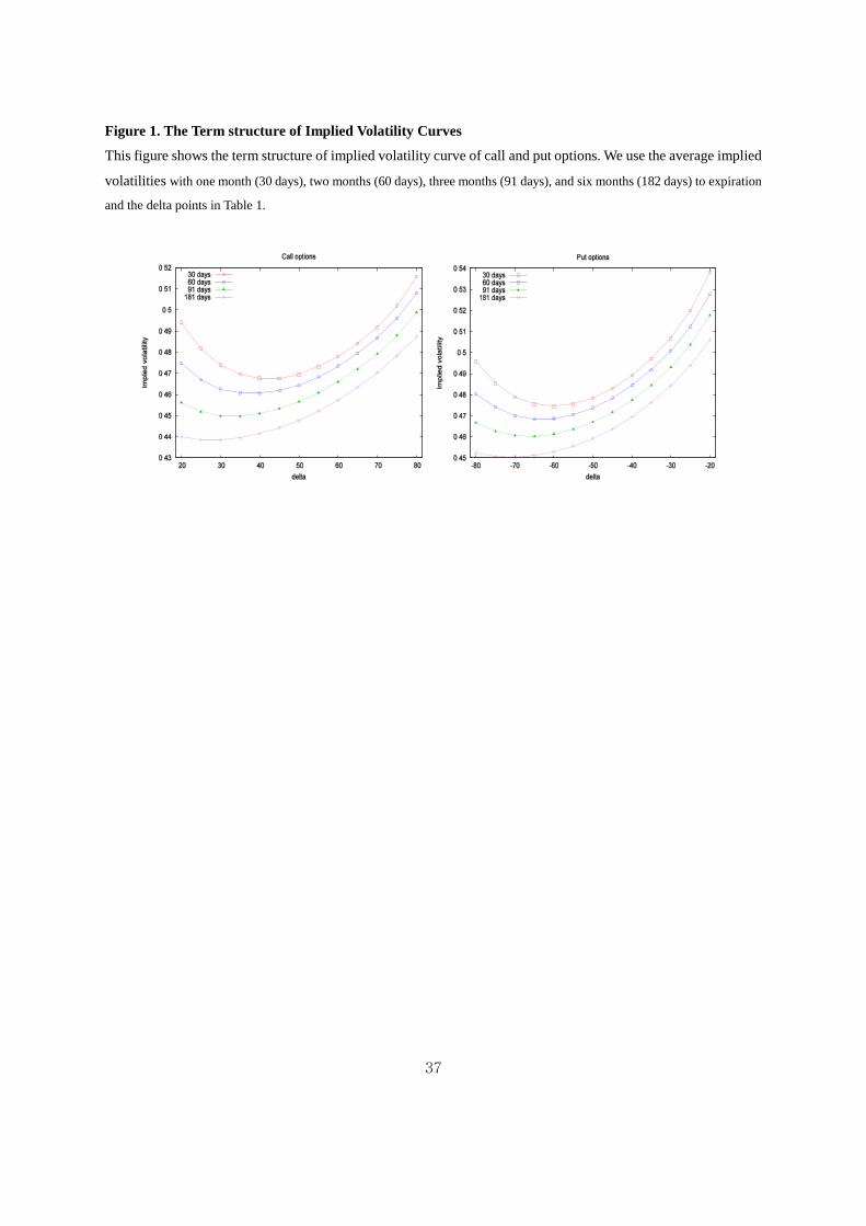
37

Figure 1. The Term structure of Implied Volatility Curves

This figure shows the term structure of implied volatility curve of call and put options. We use the average implied

volatilities with one month (30 days), two months (60 days), three months (91 days), and six months (182 days) to expiration

and the delta points in Table 1.

38

Figure 2. Average IV convexity and quintile portfolio returns

This figure shows the time-series behavior of the average 𝑂𝑟𝑡ℎ𝑜 𝑠𝑝𝑟𝑒𝑎𝑑6𝑚,1𝑚 ( 𝑂𝑟𝑡ℎ𝑜 𝑠𝑚𝑖𝑟𝑘6𝑚,1𝑚 , 𝑂𝑟𝑡ℎ𝑜 𝑐𝑜𝑛𝑣𝑒𝑥𝑖𝑡𝑦6𝑚,1𝑚) and

returns of quintile portfolios from Jan 2000 to Dec 2013. Panel A plots the monthly average 𝑂𝑟𝑡ℎ𝑜 𝑠𝑝𝑟𝑒𝑎𝑑6𝑚,1𝑚 of the quintile

portfolios and the monthly average returns of the long-short 𝑂𝑟𝑡ℎ𝑜 𝑠𝑝𝑟𝑒𝑎𝑑6𝑚,1𝑚 portfolios Q1-Q5.

Panel B plots the monthly average 𝑂𝑟𝑡ℎ𝑜 𝑠𝑚𝑖𝑟𝑘6𝑚,1𝑚 of the quintile portfolios and the monthly average returns of the long-

short 𝑂𝑟𝑡ℎ𝑜 𝑠𝑚𝑖𝑟𝑘6𝑚,1𝑚 portfolios Q1-Q5. Panel C plots the monthly average 𝑂𝑟𝑡ℎ𝑜 𝑐𝑜𝑛𝑣𝑒𝑥𝑖𝑡𝑦6𝑚,1𝑚 of the quintile portfolios

and the monthly average returns of the long-short 𝑂𝑟𝑡ℎ𝑜 𝑐𝑜𝑛𝑣𝑒𝑥𝑖𝑡𝑦6𝑚,1𝑚 portfolios Q1-Q5.

Panel A. Average 𝑂𝑟𝑡ℎ𝑜 𝑠𝑝𝑟𝑒𝑎𝑑6𝑚,1𝑚 of quintile portfolios and average returns of Q1-Q5

Panel B. Average 𝑂𝑟𝑡ℎ𝑜 𝑠𝑚𝑖𝑟𝑘6𝑚,1𝑚 of quintile portfolios and average returns of Q1-Q5

39

Panel C. Average 𝑂𝑟𝑡ℎ𝑜 𝑐𝑜𝑛𝑣𝑒𝑥𝑡𝑦6𝑚,1𝑚 of quintile portfolios and average returns of Q1-Q5