Does trading volume really explain stock returns volatility
36
Does Trading Volume Really Explain Stock Returns Volatility? by Thierry Ané 1 and Loredana Ureche-Rangau 2 1 Associate Professor at IESEG School of Management, 3 rue de la Digue, 59800 Lille, France. Phone: +33 3 20 54 58 92. Fax: +33 3 20 57 48 55. Email: [email protected] 2 Assistant Professor at IESEG School of Management, 3 rue de la Digue, 59800 Lille, France. Phone: +33 3 20 54 58 92. Fax: +33 3 20 57 48 55. Email: [email protected]
-
Upload
independent -
Category
Documents
-
view
1 -
download
0
Transcript of Does trading volume really explain stock returns volatility

Does Trading Volume Really Explain
Stock Returns Volatility?
by
Thierry Ané1
and
Loredana Ureche-Rangau2
1 Associate Professor at IESEG School of Management, 3 rue de la Digue, 59800 Lille, France. Phone: +33 3 20 54 58 92. Fax: +33 3 20 57 48 55. Email: [email protected] 2 Assistant Professor at IESEG School of Management, 3 rue de la Digue, 59800 Lille, France. Phone: +33 3 20 54 58 92. Fax: +33 3 20 57 48 55. Email: [email protected]

Abstract
Assuming that the variance of daily price changes and trading volume are
both driven by the same latent variable measuring the number of price-relevant
information arriving on the market, the Mixture of Distribution Hypothesis (MDH)
represents an intuitive and appealing explanation for the empirically observed
correlation between volume and volatility of speculative assets.
This paper investigates to which extent the temporal dependence of volatility
and volume is compatible with a MDH model through a systematic analysis of the
long memory properties of power transformations of both series.
It is found that the fractional differencing parameter of the volatility series
reaches its maximum for a power transformation around and then decreases for
other order moments while the differencing parameter of the trading volume
remains remarkably unchanged. The volatility process thus exhibits a high degree of
intermittence whereas the volume dynamic appears much smoother. The results
suggest that volatility and volume may share common short-term movements but
that their long-run behavior is fundamentally different.
75.0
Keywords: Volatility Persistence, Long Memory, Trading Volume.
JEL Classification: C13, C52, G15.
2

1. Introduction
The relations among trading volume, stock returns and price volatility, the
subject of empirical and theoretical studies over many years, have recently received
renewed attention with the increased availability of high frequency data. A vast
amount of the empirical research has documented what is now known as the
“stylized facts” about asset returns and trading volume. In particular, speculative
asset returns are found to be leptokurtic relative to the normal distribution and
exhibit a high degree of volatility persistence. The same abnormality is found for the
trading volume which also happens to be is positively correlated with squared or
absolute returns.
A meaningful approach for rationalizing the strong contemporaneous
correlation between trading volume and volatility – as measured by absolute or
squared returns – is provided by the so-called Mixture of Distribution Hypothesis
(MDH) introduced by Clark (1973). In this model, the variance of daily price changes
and trading volume are both driven by the same latent variable measuring the
number of price-relevant information arriving on the market. The arrival of
unexpected “good news” results in a price increase whereas “bad news” produces a
price decrease. Both events are accompanied by above-average trading activity in the
market as it adjusts to a new equilibrium. The absolute return (volatility) and trading
volume will thus exhibit a positive correlation due to their common dependence on
the latent information flow process.
Another successful specification for characterizing the dynamic behavior of
asset price volatility is based on the AutoRegressive Conditionally Heteroskedastic
(ARCH) model of Engle (1982) and the Generalized ARCH (GARCH) of Bollerslev
(1986). In this class of models, the conditional variance of price changes is a simple
function of past information contained in previous price changes. The autoregressive
structure in the variance specification allows for the persistence of volatility shocks,
enabling the model to capture the frequently observed clustering of similar-sized
price changes, the so-called GARCH effects.
3

These univariate time series models, however, are rather silent about the
sources of the persistence in the volatility process. In the search of the origin of these
GARCH effects, Lamoureux and Lastrapes (1990) analyze whether they can be
attributed to a corresponding time series behavior of the information arrival process
in Clark’s mixture model. Inserting the contemporaneous trading volume in the
conditional variance specification shows that this variable has significant explanatory
power and that previous price changes contain negligible additional information
when volume is included in the variance equation.
This inference, however, is based on the assumption that trading volume is
weakly exogenous, which is not adequate if price changes and trading volume are
jointly determined. As explained by Andersen (1996) it seems to be necessary to
analyze the origin of GARCH effects in a setting where trading volume is treated as
an endogenous variable. Tauchen and Pitts (1983) refined Clark’s univariate mixture
specification by including the trading volume as an endogenous variable and
proposed a Bivariate Mixture Model (BMM) in which volatility and trading volume
are jointly directed by the latent number of information arrivals. This implies that the
dynamics of both variables are restricted to depend only on the time series behavior
of the information arrival process. Hence, if the bivariate mixture models are the
correct specification, the time series of trading volume provides information about
the factor which generates the persistence in the volatility process.
Unfortunately, recent empirical studies reveal some shortcomings in the
bivariate mixture models. Lamoureux and Lastrapes (1994) show that the estimated
series of latent information arrival process does not fully account for the persistence
of stock price volatility. Similar results were obtained by Andersen (1996) and
Liesenfeld (1998) even in a context where an autoregressive structure is put on the
latent information arrival process. In order for the BMM to be able to successfully
explain the observed features of the price changes and volume series, Liesenfeld
(2001) even presents a generalized mixture model where the latent process includes
two components (the number of information arrivals and the traders’ sensitivity to
new information), both endowed with their own dynamic behavior.
4

Although from a market microstructure perspective, the BMM representation
is intuitively appealing, the absence of strong empirical support for the model seems
to suggest that volatility and trading volume have too different dynamics to be
directed by the same latent process as suggested by the BMM. It also appears that the
fundamental differences of behavior, making the BMM untenable, should be looked
for in the structure of temporal dependencies of both series.
To this respect, an extensive empirical literature has developed over the past
decade for modeling the temporal dependencies in financial markets volatility. A
common finding to emerge from most of the studies concerns the extremely high
degree of own serial dependencies in the series of absolute or squared returns.
However, the available empirical evidence regarding the dynamic dependencies in
financial market trading volume is more limited. Lobato and Velasco (2000) analyze
the long memory property for the trading volume and volatility (as measured by
squared or absolute returns) of 30 stocks composing the Dow Jones Industrial
Average index. They conclude that return volatility ( or 2tR tR ) and trading volume
(V ) possess the same long memory parameter, lending some support to Bollerslev
and Jubinski’s (1999) mixture model where a common latent process exhibiting long
memory is used.
t
In an investigation of the long-run dependencies in stock returns, Ding
Granger and Engle (1993) explain, however, that power transformations other than
unity or square have to be considered to fully characterize the long-run property of a
financial series. Considering the temporal properties of the functions qtR for
positive values of , they show that the power transformations of returns do exhibit
long memory with quite high autocorrelations for long lags and that this property is
strongest for or near 1 compared to both smaller and larger positive values.
q
1=q
The main contribution of this paper is to find out to which extent the temporal
dependence of volatility and volume of speculative assets is compatible with a MDH
model through a systematic analysis of the long memory properties of power
transformations of order of both the return and the trading volume series (i.e., q
5

qtR and V ). To this end we follow the methodology introduced in Ding, Granger
and Engle (1993) and Ding and Granger (1996): the analysis of long memory is
tantamount to studying the decay rate of the autocorrelation function. The output of
such an analysis yields the fractional integration parameter commonly denoted by .
In this paper, it is obtained through the semiparametric techniques developed by
Robinson (1994, 1995a and 1995b). The results obtained are quite surprising: whereas
the fractional differencing parameter, , reaches its maximum for and then
decreases for higher order moments in the case of the volatility, the same
differencing parameter remains remarkably unchanged in the case of the trading
volume. Hence, the volatility process appears to be more complex than the volume
process and exhibits a higher degree of intermittence
qt
d
d 75.0=q
1.
α
Restating the results in the very simple and intuitive framework developed by
Lamoureux and Lastrapes (1990), we observe that the inclusion of trading volume in
the conditional variance equation of these stocks does not change the degree of
temporal dependence. That is, it leaves the level of volatility persistence, as measured
by the sum β+ , virtually unchanged and the volume coefficient is not significant.
Trading volume is only able to explain the volatility persistence of stocks with the
lower degree of intermittence. In this situation, we recover the appealing result of
Lamoureux and Lastrapes (1990), namely the fact that volume becomes highly
significant and the volatility persistence measured by βα + decreases to zero. Our
results suggest that volatility and volume may share common short-term movements
but that their long-run behavior is fundamentally different.
In the search for improvements of the BMM framework that enable to account
for the asymmetric behavior of volume and volatility on the short- and long-run, two
competing models were recently presented in the literature. On the one hand,
Bollerslev and Jubinski (1999) find that the long-run dependencies of volume and
volatility are common but that the short-run responses to certain types of “news” are
not necessarily the same across the two variables. With a different specification,
Liesenfeld (2001) explains that the short-run volatility dynamics are directed by the 1 Broadly speaking, what we mean by intermittence is brutal movements in the volatility series.
6

information arrival process, whereas the long-run dynamics are associated with the
sensitivity to new information. On the contrary, the variation of the sensitivity to
news is largely irrelevant for the behavior of trading volume which is mainly
determined by the variation of the number of information arrivals. Our results
obtained using semiparametric methods outside this BMM framework thus lend
support to Liesenfeld’s specification in the sense that it differenciates volume and
volatility for their long-run behavior.
The remainder of this paper is organized as follows. Section 2 briefly reviews
the methodology of the Ding, Granger and Engle test. The data, the empirical
estimations and the results are presented in Section 3. An intuitive correspondence
with the MDH framework of Lamoureux and Lastrapes (1990) is discussed in Section
4 while the last section concludes.
2. Long-Run Dependencies in Volatility and Volume
In agreement with the efficient market theory, empirical studies have shown
that although stock market returns are uncorrelated at lags larger than a few
minutes, where some microstructure effects might apply, absolute and squared
returns - common measures of volatility - do exhibit long-range dependencies in
their autocorrelation function. In order to better define the notion of long memory,
we follow Robinson (1994) among others. A stationary process presents long
memory if its autocorrelation function )( jρ has asymptotically the following rate of
decay: 12)()( −≈ djjLjρ as ∞→j , (1)
where is a slowly varying function)( jL 2 and )2/1,0(∈d is the parameter governing
the slow rate of decay of the autocorrelation function. This parameter measures
the degree of long-range dependence of the series. In this context, the long memory
property of the absolute returns should be written as:
d
2 Such that 0,1)(/)(lim >∀=
∞→λλ jLjL
j.
7

12)(),( −≈ dt jjLjRρ as ∞→j . (2)
Studying a large variety of speculative assets, Taylor (1986) first highlighted the
existence of such an empirical regularity in the autocorrelation of the absolute
returns.
Applying the Granger & Newbold (1977) techniques for power transforms of
Normal distributions, Andersen & Bollerslev (1997) push the analysis one step
further and theoretically show that, in this context, any power transformation of the
absolute returns, qtR , possesses this long memory property. Namely, that:
12),( −≈ dqt jjRρ (3)
where j is large and denotes the jth information arrival process and the
hyperbolic rate of decay or the fractional differencing parameter ( 0 ). From
an empirical viewpoint, Ding, Granger and Engle (1993) use the S&P 500 stock index
to study the decay rate of the autocorrelation function when different power
transformations of the absolute returns are analyzed (i.e.,
d
2/1<< d
qtR for ).
They indeed conclude to the existence of a long memory property regardless the
value for the parameter and also show that the slowest decay rate for the
autocorrelation function is obtained for values of q close to 1.
2...,,5.0,25.0=q
q
Whatever its form, the MDH framework does not mean a causal relationship
between the variance of daily price changes and trading volume. Both variables are
assumed to be driven by the same latent process measuring the number of price-
relevant information arriving in the market. As such, it implies a common long-range
dependence in the volatility and the volume processes. If the MDH represents a
correct specification of the contemporaneous behavior of volatility and volume, the
autocorrelation function of the latter process should exhibit the same rate of decay as
the autocorrelation function of volatility as represented by tR . Hence one should
observe the following: 12),( −≈ d
t jjVρ as ∞→j and 2/10 << d , (4)
with V being the trading volume. t
8

Moreover, under some specific distributional assumptions (see Bollerslev and
Jubinski (1999)), the cross-correlations between the volatility and the trading volume
may also present the same hyperbolic decay: 12),(),( −
−− ≈≈ djttjtt jRVcorrVRcorr . (5)
One way of testing the adequacy of the MDH models is thus through an
analysis of the long memory behavior of the volatility and volume processes as well
as the rate of decay of their cross-correlations functions. In this direction, we apply
the Ding, Granger and Engle (1993) approach and do not restrict our analysis to a
single power transformation of both series. Rather, we investigate the rate of decay of
the autocorrelation functions ),( jR qtρ
4...,,5.
and for different values of the
power term (i.e., for q ). In addition to representing a new method for
testing the simultaneous behavior of volatility and volume, our approach offers the
interesting property of providing a test for the MDH that does not rely on any
parametric specification of the latent process.
),( jV qtρ
0,25.0=
In this paper, we use a semiparametric framework to estimate the degree of
fractional differencing . Although this type of approach necessarily results in an
efficiency loss compared to parametric methods (like MLE or GMM), it allows
avoiding problems resulting from model misspecifications in the parametric case
(Bollerslev and Jubinski (1999)). The approach relies on the spectrum
d
)(ωf of a
covariance stationary process , at frequency tX ω , defined by:
∫−
=π
π
ωτωωτ difX t )exp()(),cov( , (6)
with ...,1,0 ±=τ . If the series is fractionally integrated, then, for frequencies ω close
to 0 , dCf 2)( −≈ ωω as , (7) +→ 0ω
where C is a strictly positive constant. Nevertheless, the spectrum of a long memory
process has a singular feature at frequency zero as ∞=+→
)(lim0
ωω
f . Hence, instead of
assuming the knowledge of this process at all frequencies, one only establishes some
hypothesis concerning the behavior of the spectral density in the neighborhood of
9

the origin (around the low frequencies). As there is no parametric assumption about
the spectrum outside the neighborhood of the origin, the approach is called
semiparametric.
Let the process for the absolute returns or the trading volume be: tX
ttd XL η=− )1( , (8)
with being the lag operator and L tη representing a stationary and ergodic process
with a bounded spectrum, )(ωηf , at all frequencies ω . Then, the spectrum for the
process will be: tX
[ ] )()exp(1)(2
ωωω ηfif d−−−= , (9)
with )(ωηf being positive, even, continuous and bounded away from zero and from
infinity. In this framework, controls for the long memory characteristics whereas d
)(ωηf integrates the short term behavior. The only thing that we need to specify
concerning the form of the function )(ωηf is that in the neighborhood of the origin,
i.e. 0→ω ,
)0()( 2ηωω ff d−= . (10)
We then have:
[ ] )ln(2)0(ln)(ln ωω η dff −≈ , (11)
and the spectrum is approximately log-linear for the long-run frequencies.
A widely known and commonly used semiparametric estimator for based
directly on this relation is the so-called GPH log-periodogram regression estimator
introduced by Geweke and Porter-Hudak (1983)) and denoted by . It is obtained
by running the following regression:
d
GPHd̂
[ ] jjj eidI +−−−= )exp(1ln2)(ln 0 ωβω , (12)
10

where T denotes the sample size and )( jI ω is the series periodogram3 at the
Fourrier frequency,
jth
),0(/2 ππω ∈= Tjj . Hence, the logarithm of the sample
periodogram ordinates is regressed on a constant and the (lowest) Fourrier
frequencies. The GPH regression estimator is then simply calculated as being
times the estimated slope of this regression.
GPHd̂
2/1−
As )0()( 2ηωω ff d−= only works for jω close to zero, we must restrict the
regression to the Fourrier frequencies in the neighborhood of the origin. This is why
the regression is run by using only the first Fourrier frequencies close to zero (i.e. ,
), where l and are the trimming and truncation parameters.
m
m...,,2+llj ,1+= m
The consistency of this estimator is provided by Robinson (1995a and 1995b)
under regularity conditions (namely, ∞→m , ∞→l but 0→ml and 0→
Tm
()/1 ∗m
) as well
as the assumption of normality of the analyzed series. In this situation, the estimator
itself is asymptotically Gaussian, having a variance equal to ( .
However, the absolute returns
)24/2π
tR and the trading volume V , like most financial
series, violate the Gaussian assumption and invalidate the asymptotic theory for the
estimator. In order to overcome this difficulty, we thus introduce the less
restrictive estimator adopted by Andersen and Bollerslev (1997). Denoted by ,
this most robust estimator is based on the average periodogram ratio for two
frequencies close to zero as shown below:
t
GPHd̂
APd̂
[ ])ln(2
)(ˆ/)(ˆln21ˆ
τωωτ mm
APFF
d −= , (13)
where is the average periodogram, )(ˆ ωF ∑=
=m
jjI
TF
1)(2)(ˆ ωπω for frequencies
(m but m...,j ,2,1= ∞→ 0→Tm ) and 0 1<< τ . By construction, the estimated
3 2
1
1 )exp()2()( ∑=
−=T
tjtj tiXTI ωπω .
11
parameter4 is in the stationary range since it is below 1 . Moreover, Lobato and
Robinson (1997) prove that is asymptotically Gaussian for and non
normally distributed for 1 .
APd̂
APˆ
25.0=
2/
APd̂
≤ d
4/10 << d
2/14/ <
%
In the following empirical analysis, we thus use the Andersen and Bollerslev
estimator to measure the long-run dependencies in the absolute moments of
order q ( q ) of both the return and the trading volume series.
d
4...,,5.0,
3. Breaking Out the Conventional Viewpoint
The data set used for our empirical work consists in daily prices and trading
volume for 50 London Stock Exchange “blue chips” quoted between January 1990
and May 2001. All series were collected from Datastream and include
observations. To save space and to ease the presentation, results are only provided
for six stocks: Allied Domecq, Hilton GP, British Land, Barclays, Reuters GP and
Dixons GP. They are representative, however, of what is obtained for the whole
sample. Returns are calculated as differences of price logarithms and the trading
volume is also used in logarithm
2874
5.
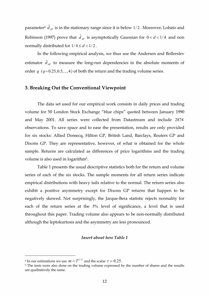
Table 1 presents the usual descriptive statistics both for the return and volume
series of each of the six stocks. The sample moments for all return series indicate
empirical distributions with heavy tails relative to the normal. The return series also
exhibit a positive asymmetry except for Dixons GP returns that happen to be
negatively skewed. Not surprisingly, the Jarque-Bera statistic rejects normality for
each of the return series at the 5 level of significance, a level that is used
throughout this paper. Trading volume also appears to be non-normally distributed
although the leptokurtosis and the asymmetry are less pronounced.
Insert about here Table 1
4 In our estimations we use and the scalar 2/1Tm = 25.0=τ . 5 The tests were also done on the trading volume expressed by the number of shares and the results are qualitatively the same.
12

Since the early work of Harris (1986 and 1987), several papers have presented
tests of the mixture of distribution hypothesis using different speculative assets and
data frequencies. However, although Harris’ tests only rely on simple predictions
emanating from the assumption that prices and volume evolve at uniform rates in
transaction times (namely, basic tests on the correlation of volume or number of
trades with prices and squared prices or else on the autocorrelation functions of these
variables), the following studies rely on specific distributional assumptions or
parameterizations for the directing process.
Indeed, in the univariate setting, returns are modeled by a subordinated
process with the traded volume regarded as a proxy for the directing process and
tests are then performed relative to specific distributional assumptions for this
variable (see Clark (1973) or Richardson and Smith (1994)). In the bivariate setting,
both returns and volume are assumed to be directed by a latent process and
empirical tests crucially depends on the selected dynamic for this variable (see
Andersen (1996) Watanabe (2000) or Liesenfeld (2001)).
In this study we try to build our tests for the MDH in a nonparametric
framework to recover the generality of Harris’ first investigations of the model. As
explained in the previous section, the MDH framework does not imply at all a causal
relationship between the variance of daily price changes and trading volume. Since
both variables are assumed to be driven by the same latent process, they must exhibit
the same long-range dependence. Hence, if the MDH represents a correct
specification of the contemporaneous behavior of volatility and volume, the
autocorrelation function of the latter process should exhibit the same rate of decay as
the autocorrelation function of volatility. The same hyperbolic decay may also be
found for the cross-correlations between the volatility and the trading.
Our tests for the adequacy of the MDH models will thus be carried out
through an analysis of the long memory behavior of the volatility and volume
processes as well as the rate of decay of their cross-correlation functions. This
approach thus provides new tests for the MDH that do not rely on any parametric
specification of the latent process.
13

Insert about here Figure 1
Figure 1 starts this analysis by a representation of the autocorrelograms
obtained for the absolute returns – our measure of volatility – and the trading
volume of six LSE stocks. Consistent with Ding and Granger (1996), the
autocorrelations present the slow, hyperbolic decay, typically found in long memory
processes. Moreover, most of these autocorrelations are positive and statistically
significant, as lying outside the Gaussian confidence bandwidths.
We already observe, however, some important differences in the behavior of
the autocorrelation function for the trading volume relative to that of the absolute
returns. The autocorrelation of absolute returns seems to die away much faster in the
case of British Land, Hilton GP, and to some extents Barclays, than it does for the
trading volume series, implying the possibility of a different long-run behavior.
Given the importance of the existence or non-existence of a common long-run
behavior of volatility and volume for the MDH model, a formal test of the presence
of long-run dependencies in both series is required. To this end, we use the so called
Lo’s R/S long-term dependence test. Lo’s (1991) modified R/S statistic for long-range
dependence in a financial series X may be defined as follows:
−−−= ∑∑
=≤≤
=≤≤
)(min)(maxˆ1),(
1111,
XXXXs
tmQk
jjTk
k
jjTk
mT
, (14)
where is a truncature parameter, m X is the sample mean (i.e. ∑=
=T
jjXT
X1
1 ) and the
quantity represents an estimator of 2,ˆ mTs ∑= j j XX ),cov( 0
2σ defined by
∑∑==
+−=T
jjj
T
jjmT mXX
Ts
11
22, ˆ)(2)(1ˆ γω , with
11)(
+−=mjmjω and
∑−
=+ −−=
jT
ijiij XXXX
T 1))((1γ̂ , Tj <≤0 . Lo computed confidence intervals for the
statistic ),()/1( TmQT , namely he uses the interval [ as the 95
acceptance region for the null hypothesis of no long-range dependence.
]862.1,809.0 %
14

To better understand the link between the R/S statistic and the fractional
integration parameter d , let us recall that when 0=m , the R/S statistic amounts to
estimating the limit of called Hurst coefficient. This coefficient,
usually denoted by
TTQ log/),0(log
H is related to the fractional integration parameter by
. 2/1−= dH
The results for Lo’s long-term dependence test are provided in Table 2. In
agreement with Lobato and Velasco (2000), for all stocks, both the absolute returns
and the trading volume series exhibit long-run dependence (i.e., 0 ) as the
statistics remain outside the 95 confidence interval. Hence one cannot reject the
MDH when tests of a similar long memory property for volatility and trading
volume are carried out with a power transformation of unity (i.e., using
2/1<< d
%
qtR and
with ). qtV 1=q
Insert about here Table 2
Although the existence of the same long-run dependence in the cross-
correlations of volatility and volume (equation (5)) requires more stringent
assumptions and thus not represent in itself a way of rejecting all possible versions of
the MDH, it remains an interesting feature to study. For our sample of six stocks,
Figure 2 shows these cross-correlation functions. We observe the same hyperbolic
decay as for the autocorrelation function of the absolute returns or the trading
volume series in the case of four stocks, lending more support to the assumption that
these series may be driven by the same latent process. For Barclays and British Land,
however, the cross-correlations are not significant since they stay inside the
confidence interval. If this cannot be regarded as such as a sufficient feature to reject
the MDH for these stocks, we may expect, if it still holds, the relation between
volatility and volume to be much weaker.
Insert about here Figure 2
15

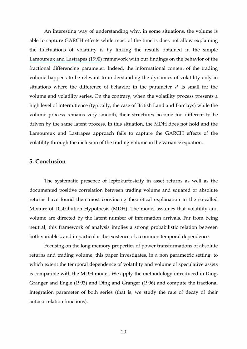
To fully compare the long-run behavior of volatility and volume, we follow
Ding, Granger and Engle (1993) and do not restrict the analysis to a single power
transformation of both series. Indeed, we now investigate the rate of decay of the
autocorrelation functions ),( jR qtρ
4...,
d
and for different values of the power
term (i.e., for ). Instead of giving all the corresponding graphs, we
summarize the results through a parameter measuring the level of long memory for
each series and each value of the power transformation . This parameter is the
degree of fractional differencing . As explained in the previous section we use the
Andersen and Bollerslev (1997) semiparametric estimator, , based on the average
periodogram ratio for two frequencies close to zero and defined in equation (13).
Figure 3 shows the obtained parameters both for the absolute returns and the trading
volume series as a function of the power transformation while Table 3 provides the
corresponding values.
),( jV qtρ
,5.0,25.0=q
q
APd̂
q
Insert about here Figure 3 and Table 3
First of all, being always in the interval , the estimated reveals the
presence of the long memory in almost all the power transformations of both the
absolute returns and the trading volume series. However, a striking feature appears:
whereas the fractional differencing parameter takes almost the same values for the
trading volume regardless of the power transformation , the results are rather
different for the volatility –measured by the absolute returns -. For the latter, the rate
of decay of the autocorrelation function has its maximum around and then
decreases, more or less rapidly, to significantly smaller values. This result was
obtained for the LSE stocks used in this study. Indeed, the rate of decay of the
autocorrelation function of the power transformation of the absolute returns always
presents a maximum for an exponent in the range [ and decreases
significantly for larger values while the same estimator remains remarkably
insensitive to the power transformation for the trading volume series.
)2/1,0( APd̂
75.0=
q
d̂
q
]1
50
q ,5.0
AP
q
16

Moreover, we observe that the difference of behavior of the degree of
fractional differencing is strongest in the case of stocks that exhibit no long-run
dependence in the cross-correlations. Indeed, the fractional integration parameter
of the volatility process decreases from to 0 for Barclays and even
from to for British Land while the estimators for the volume series remain
virtually at the same level. These stocks clearly present a very different long-term
behavior for the volatility and volume processes. Overall, the simultaneous analysis
of the fractional differencing parameter for the volatility and the trading volume
series at different power transformations clearly shows that both processes present
fundamentally different behaviors in the long-run.
APd̂ 3745.0 1705.
3048.0 0
To fully understand the difference in behavior, it seems interesting to link the
analysis of the fractional differencing parameter to the so-called intermittency of a
process. Indeed, the usual tool to analyze the local smoothness of a process X is by
computing its structure functions, namely the sample moments of its increments
(that is ( ) ),( qTttXE + where ),( TttX + is the increment of X between time t
and and ). The resulting scaling law may either be a linear function of ,
namely
T 0≥q
( )
t + q
qHT≈qTttXE + ),( where H is again the Hurst exponent (and
), or a nonlinear function of , i.e. 2/1−d=H q ( ) )),( qTttXE ≈+ (qT ζ . In the former
situation, X exhibits smooth trajectories while, in the latter situation, the process
presents a very unsmooth local structure and is said to be intermittent.
The presence of very different values for the fractional differencing parameter
when different power transformations of the absolute returns are used is thus
clearly a sign of intermittence in the volatility process. On the contrary, the trading
volume seems to be a much smoother process that might be associated with a linear
scaling law. This underlines once more the different time behavior between volatility
and volume. From the time dependency and the time aggregation viewpoints, the
volatility process appears to be much more complex than the trading volume
process.
d
17

4. Volume Versus GARCH Effects Revisited
Many empirical studies have shown that the GARCH model of Bollerslev
(1986) is particularly successful in its ability to capture the clustering of similar-sized
price changes through a conditional variance that depends on the past squared
residuals of the process. In its GARCH (1,1) form, the model corresponds to the
following equations:
tttR εµ += −1 , (15)
, (16) ),0(~...,,/ 221 tttt N σεεε −−
2 =t ωσ , (17) 21
21 −− ++ tt σβεα
where tε is the conditionally Gaussian residual and 1−tµ represents the conditional
mean. Since the focus of this section is strictly on the impact of the trading volume in
the variance equation, we simply assume an autoregressive process of order 1 for all
stocks. The degree of persistence in the volatility is measured by the sum of the
coefficients α and β .
Using the MDH framework, Lamoureux and Lastrapes (1990) argue that the
observed GARCH effects in financial time series may be explained as a manifestation
of time dependence in the rate of evolution of intraday equilibrium returns. They
suggest that the daily number of information arrivals directing the price process may
be proxied by the trading volume. Then, the focus of their analysis is to assess the
degree of volatility persistence that remains in a GARCH (1,1) model conditional on
the knowledge of the mixing variable (i.e., the trading volume). To do this, they use
the previous GARCH (1,1) model where the conditional variance equation is
replaced by the following:
t ωσ =2 . (18) ttt Vγσβεα +++ −−2
12
1
Equation (18) now models the conditional variance of returns as a GARCH (1,1)
process with the trading volume V as explanatory variable. The mixture model
predicts that
t
γ should be positive and significant. Moreover, the persistence of
variance as measured by βα + should become negligible if accounting for the
18

uneven flow of information with the trading volume explains the presence of
GARCH effects in the data.
Their empirical analysis based on actively traded stocks strongly supports
the MDH framework. The sample period used for their study is very small, however,
and does not include financial crises. Using different data and time periods, many
studies (see for instance Kamath, Chatrath and Chaudhry (1993) or Sharma,
Mougoue and Kamath (1996)) strongly question the informational power of trading
volume in the GARCH setting. Using the LSE stocks, we re-estimate the GARCH
(1,1) model without and with volume as described respectively by equations (17) and
(18). Results are summarized in Tables 4 and 5.
20
50
Insert about here Table 4 and Table 5
The estimated GARCH (1,1) models without volume all support the existence
of a strong persistence in the volatility process with a sum of coefficients α and β
always above . Results of the inclusion of volume as an explanatory variable in
the variance equation, however, provide mitigated conclusions, not entirely rejecting
the Lamoureux and Lastrapes (1990) findings nor giving them an unconditional
support. Indeed, for two stocks, namely Allied Domecq and Hilton GP, the trading
volume has an important explanatory power. When included in the conditional
variance equation, the coefficient
9.0
γ is significantly positive and the persistence in
volatility as measured by βα + is much smaller. For two other stocks, namely
Reuters GP and Dixons GP, the trading volume has a limited explanatory power:
even if the volume coefficient is significantly positive, GARCH effects are almost the
same and the persistence in volatility does not change significantly6. Finally, for the
last two stocks, namely British Land and Barclays, the trading volume does not
explain the volatility at all: the coefficient γ is not statistically significant and the
persistence in volatility is not affected by the inclusion of volume in the equation.
6 This is the most common result that we had on the whole sample of the 50 LSE stocks.
19
An interesting way of understanding why, in some situations, the volume is
able to capture GARCH effects while most of the time is does not allow explaining
the fluctuations of volatility is by linking the results obtained in the simple
Lamoureux and Lastrapes (1990) framework with our findings on the behavior of the
fractional differencing parameter. Indeed, the informational content of the trading
volume happens to be relevant to understanding the dynamics of volatility only in
situations where the difference of behavior in the parameter is small for the
volume and volatility series. On the contrary, when the volatility process presents a
high level of intermittence (typically, the case of British Land and Barclays) while the
volume process remains very smooth, their structures become too different to be
driven by the same latent process. In this situation, the MDH does not hold and the
Lamoureux and Lastrapes approach fails to capture the GARCH effects of the
volatility through the inclusion of the trading volume in the variance equation.
d
5. Conclusion
The systematic presence of leptokurtosicity in asset returns as well as the
documented positive correlation between trading volume and squared or absolute
returns have found their most convincing theoretical explanation in the so-called
Mixture of Distribution Hypothesis (MDH). The model assumes that volatility and
volume are directed by the latent number of information arrivals. Far from being
neutral, this framework of analysis implies a strong probabilistic relation between
both variables, and in particular the existence of a common temporal dependence.
Focusing on the long memory properties of power transformations of absolute
returns and trading volume, this paper investigates, in a non parametric setting, to
which extent the temporal dependence of volatility and volume of speculative assets
is compatible with the MDH model. We apply the methodology introduced in Ding,
Granger and Engle (1993) and Ding and Granger (1996) and compute the fractional
integration parameter of both series (that is, we study the rate of decay of their
autocorrelation functions).
20

The results obtained are quite surprising: whereas the fractional differencing
parameter reaches its maximum for power transformations around q and then
decreases for higher order moments in the case of the volatility, the same
differencing parameter remains remarkably unchanged in the case of the trading
volume. The volatility process thus exhibits a high degree of intermittence whereas
the volume dynamic appears much smoother.
75.0=
Reformulating the results in the very intuitive framework introduced by
Lamoureux and Lastrapes (1990), we obtain that stocks for which the trading volume
has virtually no explanatory power relative to the GARCH effects also correspond to
those for which the difference in the fractional parameters of volume and volatility is
the strongest.
The results suggest that volatility and volume may share common short-term
movements but that their long-run behavior is fundamentally different. This leaves
an open window for researchers willing to re-discuss the volatility-volume
relationship.
21

6. References
Andersen, T. G., 1996. Return Volatility and Trading Volume: An Information Flow
Interpretation of Stochastic Volatility. The Journal of Finance, 60, 169-204.
Andersen, T. G., and T., Bollerslev, 1997. Heterogeneous Information Arrivals and
Return Volatility Dynamics: Uncovering the Long-Run in High Frequency Returns.
The Journal of Finance, 52, 975-1005.
Bollerslev, T., 1986. Generalized Autoregressive Conditional Heteroskedasticity.
Journal of Econometrics, 31, 307-327.
Bollerslev, T., and D., Jubinski, 1999. Equity Trading Volume and Volatility: Latent
Information Arrivals and Common Long-Run Dependence. Journal of Business and
Economic Statistics, 17, 1, 9-21.
Clark, P.K., 1973; A Subordinated Stochastic Process Model with Finite Variance for
Speculative Prices. Econometrica, 41, 135-156.
Ding, Z., and C.W.J., Granger, 1996. Varieties of Long Memory Models. Journal of
Econometrics, 73, 61-77.
Ding, Z., C.W.J., Granger, and R.F., Engle, 1993. A Long Memory Property of Stock
Market Returns and a New Model. Journal of Empirical Finance, 1, 83-106.
Engle, R.F., 1982. Autoregressive Conditional Heteroskedasticity with Estimates of
the Variance of U.K. Inflation, Econometrica, 50, 987-1008.
Geweke, J., and S. Porter-Hudak, 1983. The Estimation and Application of Long-
Memory Time Series Models. Journal of Time Series Analysis, 4, 221-238.
22

Granger, C.W.J, and P., Newbold, 1977. Forecasting Economic Time-Series. Economic
Theory and Mathematical Economics, Academic Press.
Harris, L., 1986. Cross-Security Tests of the Mixture of Distributions Hypothesis.
Journal of Financial and Quantitative Analysis, 21, 1, 39-46.
Harris, L. 1987. Transaction Data Tests of the Mixture of Distributions Hypothesis.
Journal of Financial and Quantitative Analysis, 22, 2, 127-141.
Kamath, R., A., Chatrah and M. Chaudhry, 1993. The Time Dependence in Return
Generating Processes: Volume Versus ARCH and GARCH Effects in Thailand. The
International Journal of Finance, 6,1, 613-624.
Lamoureux, C.G., and W., Lastrapes, 1990. Heteroskedasticity in Stock Return Data:
Volume versus GARCH Effects. The Journal of Finance, 45, 221-229.
Lamoureux, C.G., and W., Lastrapes, 1994. Endogeneous Trading Volume and
Momentum in Stock Return Volatility. Journal of Business and Economic Statistics, 16,
101-109.
Liesenfeld, R., 1998. Dynamic Bivariate Mixture Models: Modeling the Behavior of
Prices and Trading Volume. Journal of Business and Economic Statistics, 18, 101-109.
Liesenfeld, R., 2001. A Generalized Bivariate Mixture Model for Stock Price Volatility
and Trading Volume. Journal of Econometrics, 104, 141-178.
Lo, A.W., 1991. Long Turn Memory in Stock Market Prices, Econometrica, 59, 1279-
1313.
Lobato, I., and C., Velasco, 2000. Long Memory in Stock Market Trading Volume.
Journal of Business and Economic Statistics, 18, 410-427.
23

Lobato, I., and P.M., Robinson, 1996. Averaged Periodogram Estimation of Long
Memory. Journal of Econometrics, 73, 303-324
Lobato, I., and P.M., Robinson, 1997. A Nonparametric Test for I(0). LSE STICERD
Discussion Paper, EM/97/342.
Richardson, M., and T., Smith, 1994. A Direct Test of the Mixture-of-Distribution
Hypothesis: Measuring the Daily Flow of Information. Journal of Financial and
Quantitative Analysis, 29, 101-116.
Robinson, P.M., 1994. Semiparametic Analysis of Long-Memory Time Series. The
Annals of Statistics, 22, 515-539.
Robinson, P.M., 1995a. Gaussian Semiparametric Estimation of Long-Range
Dependence. The Annals of Statistics, 23, 1630-1661.
Robinson, P.M., 1995b. Log Periodogram Regression of Time Series with Long Range
Dependence. The Annals of Statistics, 23, 1048-1072.
Robinson, P.M., 1995. Gaussian Semiparametric Estimation of Long-Range
Dependence. The Annals of Statistics, 23, 1630-1661.
Sharma, J., M. Mougoue and R. Kamath, 1996. Heteroscedasticity in Stock Market
Indicator Return Data: Volume Versus GARCH Effects. Applied Financial Economics, 6,
337-342.
Tauchen, G., and M., Pitts, 1983. The Price Variability – Volume Relationship on
Speculative Markets. Econometrica, 51, 2, 485-505.
Taylor, S.J., 1986. Modelling Financial Time Series. John Wiley and Sons, Chichester.
24

Watanabe, T., 2000. Bayesian Analysis of Dynamic Bivariate Mixture Models: Can
They Explain the Behavior of Returns and Trading Volume? Journal of Business and
Economic Statistics, 18, 2, 199-210.
25

Figure 1
Autocorrelograms for the Absolute Returns - Volatility - and Traded Volume.
We plot the autocorrelations of the absolute returns – as a measure of volatility – and
the trading volume of six stocks traded on the London Stock Exchange Market, for
lag 1 to lag . For all stocks we see the slow hyperbolic decay, which characterises
long memory processes, i.e.
20012),( −≈ d
t jjRρ and as and
. The autocorrelations remain above the confidence interval
(
12),( −≈ dt jjVρ
%95
∞→j
2/10 << d
T/961± . ) for long lags (even as long as for some stocks). However, the
autocorrelation of absolute returns seems to die out much faster in the case of British
Land, Hilton GP and even Barclays compared to the trading volume series.
200
26

Allied Domecq
-0.15
-0.05
0.05
0.15
0.25
0.35
0.45
0.55
0 25 50 75 100 125 150 175 200
Confidence interval Confidence interval Abs returns Volume
Hilton GP
-0.15
-0.05
0.05
0.15
0.25
0.35
0.45
0.55
0 25 50 75 100 125 150 175 200
Confidence interval Confidence interval Abs returns Volume
British Land
-0.15
-0.05
0.05
0.15
0.25
0.35
0.45
0.55
0 25 50 75 100 125 150 175 200
Confidence interval Confidence interval Abs returns Volume
Barclays
-0.15
-0.05
0.05
0.15
0.25
0.35
0.45
0.55
0 25 50 75 100 125 150 175 200
Confidence interval Confidence interval Abs returns Volume
Dixons GP
-0.15
-0.05
0.05
0.15
0.25
0.35
0.45
0.55
0 25 50 75 100 125 150 175 200
Confidence interval Confidence interval Abs returns Volume
Reuters GP
-0.15
-0.05
0.05
0.15
0.25
0.35
0.45
0.55
0 25 50 75 100 125 150 175 200
Confidence interval Confidence interval Abs returns Volume
27

Figure 2
Cross-correlations of the Absolute Returns - Volatility - and Traded Volume.
We analyze the cross-correlations functions of volatility and traded volume for the
six stocks. The straight line corresponds to ),( jtt VRcorr − and the dotted one to
),( jtt RVcorr − . The graphs show the same hyperbolic decay as for the
autocorrelation functions of the absolute returns and volume, i.e. 12),(),( −
−− ≈≈ djttjtt jRVcorrVRcorr . Nevertheless, for Barclays and British Land
the cross-correlations are not significant, as they lie inside the 95 Gaussian
confidence interval.
%
28

Allied Domecq
-0.1
0
0.1
0.2
0.3
0.4
0.5
0 20 40 60 80 100 120 140 160 180 200
Hilton GP
-0.1
0
0.1
0.2
0.3
0.4
0.5
0 20 40 60 80 100 120 140 160 180 200
British Land
-0.1
0
0.1
0.2
0.3
0.4
0.5
0 20 40 60 80 100 120 140 160 180 200
Barclays
-0.1
0
0.1
0.2
0.3
0.4
0.5
0 20 40 60 80 100 120 140 160 180 200
Dixons GP
-0.1
0
0.1
0.2
0.3
0.4
0.5
0 20 40 60 80 100 120 140 160 180 200
Reuters GP
-0.1
0
0.1
0.2
0.3
0.4
0.5
0 20 40 60 80 100 120 140 160 180 200
29

Figure 3
Fractional Differencing Parameter and Power Transformation q . d
Figure 3 investigates the rate of decay of the autocorrelation functions ),( jR qtρ and
for different values of the power term (i.e., for ),( jV qtρ 2...,,5.0,25.0=q ). The fractional
differencing parameter is calculated using the semiparameter estimator of Andersen and
Bollerslev (1997) based on the average periodogram ratio for two frequencies close to zero,
. The fractional differencing parameter d takes almost the same values for the
trading volume regardless of the power transformation q for the volume (linear dotted
line) whereas the graph shows a humped shape for the volatility. For the latter, after a
maximum value around , the fractional differencing parameter decreases to
significantly smaller values for superior values of the power transform. The decrease is
very substantial in the case of British Land and Barclays.
APd̂ APˆ
75.0=q
30

Allied Domecq
0.00
0.05
0.10
0.15
0.20
0.25
0.30
0.35
0.40
0.45
0.50
00.25 0.5 0.75
11.25 1.5 1.75
22.25 2.5 2.75
33.25 3.5 3.75
4
d volatility d volume
Hilton GP
0.00
0.05
0.10
0.15
0.20
0.25
0.30
0.35
0.40
0.45
0.50
00.25 0.5 0.75
11.25 1.5 1.75
22.25 2.5 2.75
33.25 3.5 3.75
4
d volatility d volume
British Land
0.00
0.05
0.10
0.15
0.20
0.25
0.30
0.35
0.40
0.45
0.50
00.25 0.5 0.75
11.25 1.5 1.75
22.25 2.5 2.75
33.25 3.5 3.75
4
d volatility d volume
Barclays
0.00
0.05
0.10
0.15
0.20
0.25
0.30
0.35
0.40
0.45
0.50
00.25 0.5 0.75
11.25 1.5 1.75
22.25 2.5 2.75
33.25 3.5 3.75
4
d volatility d volume
Dixons GP
0.00
0.05
0.10
0.15
0.20
0.25
0.30
0.35
0.40
0.45
0.50
00.25 0.5 0.75
11.25 1.5 1.75
22.25 2.5 2.75
33.25 3.5 3.75
4
d volatility d volume
Reuters GP
0.00
0.05
0.10
0.15
0.20
0.25
0.30
0.35
0.40
0.45
0.50
00.25 0.5 0.75
11.25 1.5 1.75
22.25 2.5 2.75
33.25 3.5 3.75
4
d volatility d volume
31

Table 1
Descriptive Statistics for Daily Stock Returns and Traded Volume.
Descriptive statistics of six stocks traded on the London Stock Exchange over the
period January 1990 to May 2001 are presented in Table II. For our analysis, we use
both returns measured as )/ln(100 1−×= ttt PPR and traded volumes expressed in
logarithm. The number of observations for the period of analysis is T . The
confidence interval for a test of normality is given by
2874=
%95 T/6*96.1± for the sample
skewness and T/24*96.1±3 for the sample kurtosis. We also provide the Jarque-
Bera test for normality. We use * to indicate significance at the 5 percent level.
Mean 0.0583 Mean 9.5956 Mean 0.0101 Mean 6.6278
Variance 3.8507 Variance 0.3666 Variance 3.3366 Variance 1.3652
Skewness 0.1994* Skewness -0.0022 Skewness 0.5253* Skewness -0.9393*
Kurtosis 6.0121* Kurtosis 4.4811* Kurtosis 10.4855* Kurtosis 4.5546*
Jarque-Bera 1105.50* Jarque-Bera 262.70* Jarque-Bera 6842.22* Jarque-Bera 712.04*
Mean 0.0683 Mean 8.7848 Mean 0.0147 Mean 8.1345
Variance 5.9235 Variance 0.7891 Variance 2.8547 Variance 0.4683
Skewness -0.2449* Skewness -0.9453* Skewness 0.3021* Skewness -0.1714*
Kurtosis 11.3915* Kurtosis 5.8394* Kurtosis 10.6184* Kurtosis 4.5383*
Jarque-Bera 8461.31* Jarque-Bera 1393.59* Jarque-Bera 6994.08* Jarque-Bera 297.47*
Mean -0.0097 Mean 8.1169 Mean 0.0514 Mean 8.2072
Variance 5.3381 Variance 0.5798 Variance 5.6882 Variance 0.4961
Skewness 0.3372* Skewness 0.0893 Skewness 0.1004* Skewness -0.2285*
Kurtosis 8.8465* Kurtosis 3.7208* Kurtosis 11.1163* Kurtosis 3.8169*
Jarque-Bera 4147.77* Jarque-Bera 66.05 Jarque-Bera 7893.42* Jarque-Bera 104.94*
Returns Volume
Returns Volume
Returns Volume
Hilton GP Reuters GP
Returns Volume
Descriptive Statistics
Barclays British Land
Allied DomecqDixons GP
Returns VolumeReturns Volume
32

Table 2
Lo’s Long Term Dependence Test for Absolute Returns and Traded Volume.
Lo’s (1991) modified R/S statistic for long-range dependence is presented in Table 2 to formally test the presence of long-term
dependence in absolute returns and trading volume. In agreement with Lobato and Velasco (2000), for all stocks, both the absolute
returns and the trading volume series exhibit long-run dependence (i.e., 2/10 << d ) as the statistics remain outside the
confidence interval.
%95
m Q(m,T) m Q(m,T) m Q(m,T) m Q(m,T) m Q(m,T) m Q(m,T)
2 5.4030* 2 4.4180* 2 5.6072* 2 5.3139* 2 4.0261* 2 7.0982*
5 4.5412* 5 3.8087* 5 4.8528* 5 4.6051* 5 3.5078* 5 5.8891*
8 4.0459* 8 3.4737* 8 4.3695* 6 4.4541* 8 3.1843* 10 4.8485*
10 3.7990* 10 3.3175* 10 4.1191* 10 4.0039* 10 3.0232* 12 4,5691*
m Q(m,T) m Q(m,T) m Q(m,T) m Q(m,T) m Q(m,T) m Q(m,T)
12 3.1361* 12 5.5628* 10 4.0667* 10 4.3217* 12 3.6933* 15 4.1161*
15 2.9444* 15 5.1158* 12 3.8808* 12 4.1165* 15 3.4313* 17 3.9697*
19 2.7485* 20 4.5749* 13 3.8003* 16 3.8049* 19 3.1700* 21 3.7207*
22 2.6268* 22 4.4050* 15 3.6546* 18 3.6789* 22 3.0151* 24 3.5685*
Hilton GP Reuters GP
Barclays British Land Dixons GP Allied Domecq
Barclays British Land Dixons GP Allied Domecq
Absolute Returns
Trading Volume
Lo's Long Term Dependence Test
Hilton GP Reuters GP
33

Table 3
Decay Rate of the Autocorrelation Functions of Absolute Power Transformations for Returns and Volume.
To gauge the influence of the power transformation on the decay rate of the autocorrelation functions q ),( jR qtρ
APd̂
and ,
Table 3 presents the values of the obtained Andersen and Bollerslev (1997) fractional differencing parameters both for power
transformations of the absolute returns (volatility) and the trading volume when
),( jV qtρ
4...,,5.0,25.0=q .
q Volatility Volume Volatility Volume Volatility Volume Volatility Volume Volatility Volume Volatility
0.25 0.3745 0.3507 0.3048 0.4476 0.3996 0.3353 0.2927 0.3807 0.3465 0.3489 0.41220.5 0.3883 0.3504 0.3111 0.4485 0.4253 0.3346 0.3327 0.3824 0.3579 0.3495 0.41770.75 0.3872 0.3499 0.3129 0.4491 0.4292 0.3336 0.3404 0.3840 0.3581 0.3500 0.41841 0.3813 0.3494 0.3089 0.4496 0.4273 0.3324 0.3392 0.3855 0.3543 0.3504 0.41681.25 0.3725 0.3488 0.2987 0.4500 0.4226 0.3311 0.3331 0.3868 0.3478 0.3507 0.41341.5 0.3616 0.3482 0.2814 0.4503 0.4161 0.3296 0.3236 0.3881 0.3393 0.3509 0.40841.75 0.3492 0.3476 0.2568 0.4505 0.4079 0.3280 0.3116 0.3893 0.3291 0.3510 0.40212 0.3355 0.3469 0.2257 0.4506 0.3983 0.3263 0.2975 0.3904 0.3176 0.3510 0.39452.25 0.3203 0.3461 0.1903 0.4506 0.3875 0.3244 0.2820 0.3914 0.3055 0.3510 0.38572.5 0.3038 0.3453 0.1533 0.4505 0.3755 0.3225 0.2659 0.3924 0.2931 0.3509 0.37552.75 0.2857 0.3444 0.1176 0.4504 0.3626 0.3205 0.2495 0.3933 0.2812 0.3507 0.36403 0.2659 0.3435 0.0851 0.4502 0.3490 0.3184 0.2334 0.3942 0.2700 0.3505 0.35133.25 0.2442 0.3425 0.0571 0.4500 0.3347 0.3163 0.2180 0.3950 0.2597 0.3502 0.33743.5 0.2208 0.3414 0.0338 0.4497 0.3201 0.3141 0.2034 0.3957 0.2505 0.3499 0.32253.75 0.1959 0.3404 0.0149 0.4494 0.3053 0.3118 0.1897 0.3965 0.2424 0.3496 0.30704 0.1703 0.3392 0.0000 0.4490 0.2906 0.3095 0.1770 0.3971 0.2353 0.3493 0.2911
Reute
Rate of Decay for Absolute Power Transformations of Returns and Traded Volume
Barclays British Land Dixons GP Allied Domencq Hilton GP
34

Table 4
GARCH (1,1) Parameter Estimates without Trading Volume.
We use the LSE “blue chips” stocks over the period January 1990 to May 2001 to
estimate by maximum likelihood the parameters of a GARCH (1,1) model without
volume. Results for the six stocks discussed in this paper are presented in Table 4
where heteroskedastic-consistent t-values are also provided in parenthesis. All stocks
exhibit a high level of volatility persistence as measured by the sum βα + .
ω α β α + β
Barclays 0.0482* 0.0805* 0.9085* 0.9889
(3.297) (6.542) (64.38)
British Land 0.0678* 0.0986* 0.8875* 0.9860
(3.955) (7.64) (61.67)
Dixons GP 0.1109* 0.0867* 0.8988* 0.9853
(3.949) (6.68) (59.97)
Allied Domecq 0.0897* 0.0861* 0.8830* 0.9690
(4.241) (6.569) (49.24)
Hilton GP 0.0572* 0.0596* 0.9318* 0.9912
(3.529) (7.373) (106.5)
Reuters GP 0.0440* 0.0826* 0.9135* 0.9960
(3.338) (6.501) (71.69)
GARCH ( 1, 1 ) Model without Trading Volume
35

Table 5
GARCH (1,1) Parameter Estimates with Trading Volume.
Table 5 follows the work of Lamoureux and Lastrapes (1990) and presents the
parameter estimates of a GARCH (1,1) model that includes the trading volume as
explanatory variable in the variance equation. Again, the study was done on 50 LSE
“blue chips” stocks even though results are only presented for six stocks. Significance
of the parameters is measured by the heteroskedastic-consistent t-values. The last
column gives the level of volatility persistence by the sum βα + when volume has
been included in the equation.
ω α β γ α + β
Barclays -0.5591 0.0962* 0.8825* 0.0676 0.97853
(-1.780) (5.952) (40.31) (1.903)
British Land 0.0284 0.0999* 0.8849* 0.0066 0.98467
(0.5027) (7.429) (56.55) (0.7127)
Dixons GP -1.0955* 0.1237* 0.8364* 0.1557* 0.95996
(-4.411) (6.624) (31.59) (4.515)
Allied Domecq -2.8069* 0.1920* 0.5828* 0.4213* 0.7746
(-10.98) (8.710) (16.03) (11.13)
Hilton GP -7.4209* 0.2121* 0.2183* 1.2577* 0.43022
(-26.99) (8.326) (9.618) (26.92)
Reuters GP -1.4614* 0.1200* 0.8462* 0.2023* 0.96593
(-4.562) (7.591) (37.94) (4.519)
GARCH ( 1, 1 ) Model with Trading Volume
36