Symmetry, Integrability and Geometry: Methods and Applications SIGMA 13 (2017), 008, 23 pages

Classical and Quantum Superintegrability

of Stackel Systems

Maciej B LASZAK † and Krzysztof MARCINIAK ‡

† Faculty of Physics, Division of Mathematical Physics,A. Mickiewicz University, Poznan, Poland

E-mail: blaszakm@amu.edu.pl

‡ Department of Science and Technology, Campus Norrkoping, Linkoping University, Sweden

E-mail: krzma@itn.liu.se

Received September 18, 2016, in final form January 19, 2017; Published online January 28, 2017

https://doi.org/10.3842/SIGMA.2017.008

Abstract. In this paper we discuss maximal superintegrability of both classical and quan-tum Stackel systems. We prove a sufficient condition for a flat or constant curvatureStackel system to be maximally superintegrable. Further, we prove a sufficient conditionfor a Stackel transform to preserve maximal superintegrability and we apply this conditionto our class of Stackel systems, which yields new maximally superintegrable systems asconformal deformations of the original systems. Further, we demonstrate how to performthe procedure of minimal quantization to considered systems in order to produce quantumsuperintegrable and quantum separable systems.

Key words: Hamiltonian systems; classical and quantum superintegrable systems; Stackelsystems; Hamilton–Jacobi theory; Stackel transform

2010 Mathematics Subject Classification: 70H06; 70H20; 81S05; 53B20

1 Introduction

A real-valued function h1 on a 2n-dimensional manifold (phase space) M = T ∗Q is calleda classical maximally superintegrable Hamiltonian if it belongs to a set of n Poisson-commutingfunctions h1, . . . , hn (constants of motion, so that {hi, hj} = 0 for all i, j = 1, . . . , n) andfor which there exist n − 1 additional functions hn+1, . . . , h2n−1 on M that Poisson-commutewith the Hamiltonian h1 and such that all the functions h1, . . . , h2n−1 constitute a functionallyindependent set of functions. Analogously, a quantum maximally superintegrable Hamiltonianis a self-adjoint differential operator h1 acting in an appropriate Hilbert space of functions onthe configuration space Q (square integrable with respect to some metric) belonging to a set of ncommuting self-adjoint differential operators h1, . . . , hn acting in the same Hilbert space (so that[hi, hj ] = 0 for all i, j = 1, . . . , n) and such that it also commutes with an additional set of n− 1

differential operators hn+1, . . . , h2n−1 of finite order. Besides, in analogy with the classical case,it is required that all the operators h1, . . . , h2n−1 are algebraically independent [19]. Throughoutthe paper it is tacitly assumed that n > 1 as the case n = 1 is not interesting from the point ofview of our theory.

This paper is devoted to n-dimensional maximally superintegrable classical and quantumStackel systems with all constants of motion quadratic in momenta. Although superintegrablesystems of second order, both classical and quantum, have been intensively studied (see forexample [1, 2, 11, 14, 16, 17] and the review paper [19]), nevertheless all the results aboutsuperintegrable Stackel systems (including the important classification results) were mainlyrestricted to two or three dimensions or focused on the situation when the Hamiltonian isa sum of one degree of freedom terms and therefore itself separates in the original coordinate

2 M. B laszak and K. Marciniak

system (see for example [3, 12] or [15]). Here we present some general results concerning n-dimensional classical separable superintegrable systems in flat spaces, constant curvature spacesand conformally flat spaces. We also present how to separately quantize all considered classicalsystems. We stress, however, that we do not develop spectral theory of the obtained quantumsystems, as it requires a separate investigation.

The paper is organized as follows. In Section 2 we briefly describe – following previous refe-rences, for example [18] and [5] – flat and constant curvature Stackel systems that we considerin this paper. In Section 3 we prove (Theorem 3.3) a sufficient condition for this class of Stackel

system to be maximally superintegrable by finding a linear in momenta function P =n∑s=1

ysps

on M such that {h1, P} = c (it also means that the vector field Y =n∑s=1

ys ∂∂qs

in P is a Killing

vector for the metric generated by h1) which yields additional n− 1 functions hn+i = {hi+1, P}commuting with h1 and thus turning h1 into a maximally superintegrable Hamiltonian. In Sec-tion 4 we briefly remind the notion of Stackel transform (a functional transform that preservesintegrability) and prove (Theorem 4.2) conditions that guarantee that a Stackel transform trans-forms maximally superintegrable system into another maximally superintegrable system (i.e.,preserves maximal superintegrability). In Section 5 we apply this result to our class of maximallysuperintegrable Stackel systems, obtaining Theorem 5.2 stating when the Stackel transform ap-plied to the considered class of systems yields a Stackel system that is flat, of constant curvatureor conformally flat. We also demonstrate (Theorem 5.4) that the additional integrals hn+i ofsystems after Stackel transform can be obtained in two equivalent ways. Section 6 is devotedto the procedure of minimal quantization of considered Stackel systems. As the procedure ofminimal quantization depends on the choice of the metric on the configurational space, we re-mind first the result obtained in [5] explaining how to choose the metric in which a minimalquantization is performed so that the integrability of the quantized system is preserved (Theo-rem 6.1) and then apply Lemma 6.3 to obtain Corollary 6.4 stating under which conditions theprocedure of minimal quantization of a classical Stackel system, considered in previous sections,yields a quantum superintegrable and quantum separable system. The paper is furnished withseveral examples that continue throughout sections. The examples are all 3-dimensional in orderto make the formulas readable but our theory works in arbitrary dimension.

2 A class of flat and constant curvature Stackel systems

Let us first introduce the class of Hamiltonian systems that we will consider in this paper.Consider a 2n-dimensional manifold M = T ∗Q (we remind the reader that n > 1) equippedwith a set of (smooth) coordinates (λ, µ) = (λ1, . . . , λn, µ1, . . . , µn) defined on an open dense setof M and such that λ are the coordinates on the base manifold Q while µ are fibre coordinates.Define the bivector

Π =

n∑i=1

∂

∂λi∧ ∂

∂µi. (2.1)

Then the bivector Π satisfies the Jacobi identity so it becomes a Poisson operator (Poissontensor), our manifold M becomes Poisson manifold and the coordinates (λ, µ) become Darboux(canonical) coordinates for the Poisson tensor (2.1). Consider also a set of n algebraic equationson M

σ(λi) +n∑j=1

hjλγji =

1

2f(λi)µ

2i , i = 1, . . . , n, γi ∈ N, (2.2)

Classical and Quantum Superintegrability of Stackel Systems 3

where we normalize γn = 0 and where σ and f are arbitrary functions of one variable. Therelations (2.2) constitute a system of n equations linear in the unknowns hj . Solving theseequations with respect to hj we obtain n functions hj = hj(λ, µ) on M of the form

hj =1

2µTAj(λ)µ+ Uj(λ), j = 1, . . . , n, (2.3)

where we denote λ = (λ1, . . . , λn)T and µ = (µ1, . . . , µn)T . The functions hj can be interpretedas n quadratic in momenta µ Hamiltonians on the manifold M = T ∗Q while the n × n sym-metric matrices Aj(λ) can be interpreted as n twice contravariant symmetric tensors on Q. TheHamiltonians hj commute with respect to Π

{hi, hj} ≡ Π(dhi, dhj) = 0 for all i, j = 1, . . . , n,

since the right-hand sides of relations (2.2) commute. Thus, the Hamiltonians in (2.3) constitutea Liouville integrable Hamiltonian system (as they are moreover functionally independent). TheHamiltonians (2.3) constitute a wide class of the so called Stackel systems [24] on M while therelations (2.2) are called separation relations [23] of this system. This is the class we willconsider throughout our paper. Note that by the very construction of hi the variables (λ, µ)are separation variables for all the Hamiltonians in (2.3) in the sense that the Hamilton–Jacobiequations associated with hj admit a common additively separable solution.

Let us now treat the matrix A1 as a contravariant form of a metric tensor on Q: A1 = G,which turns Q into a Riemannian space. The covariant form of G will be denoted by g (so thatg = G−1). It turns out that the (1, 1)-tensors Kj defined by

Kj = Ajg, j = 1, . . . , n (2.4)

(so that Aj = KjG and K1 = I) are Killing tensors of the metric g.In this article we will focus on a particular subclass of systems (2.2) that is given by the

separation relations

σ(λi) +

n∑j=1

hjλn−ji =

1

2f(λi)µ

2i , i = 1, . . . , n, (2.5)

(systems of the above class are known in literature as Benenti systems) where moreover

f(λ) =

m∑j=0

bjλj , bj ∈ R, m ∈ {0, . . . , n+ 1}, (2.6)

σ(λ) =∑k∈I

αkλk, αk ∈ R, (2.7)

where I ⊂ Z is some finite index set (i.e., σ is a Laurent polynomial). Note that takingk ∈ {0, . . . , n − 1} will only yield trivial terms in solutions (2.3) of (2.5), see the end of thissection. Also, the parameters αk will play a crucial roll in the sequel, when we discuss theStackel transform of the above systems. The metric tensor G attains in this case, due to (2.6),the form

G =

m∑j=0

bjGj =

m∑j=0

bjLjG0, (2.8)

where L = diag(λ1, . . . , λn) is a (1, 1)-tensor (the so called special conformal Killing tensor, seefor example [10]) on Q, while

Gj = diag

(λj1∆1

, . . . ,λjn∆n

), j ∈ Z, ∆i =

∏j 6=i

(λi − λj). (2.9)

4 M. B laszak and K. Marciniak

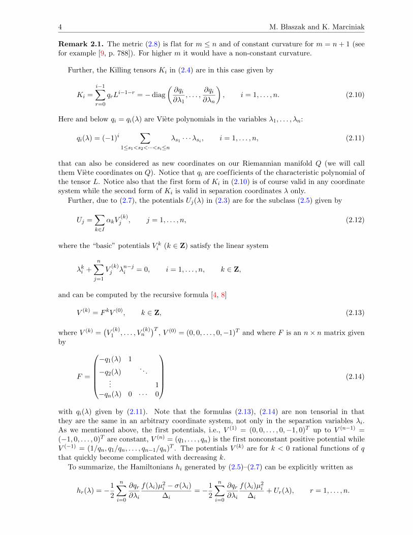
Remark 2.1. The metric (2.8) is flat for m ≤ n and of constant curvature for m = n+ 1 (seefor example [9, p. 788]). For higher m it would have a non-constant curvature.

Further, the Killing tensors Ki in (2.4) are in this case given by

Ki =i−1∑r=0

qrLi−1−r = −diag

(∂qi∂λ1

, . . . ,∂qi∂λn

), i = 1, . . . , n. (2.10)

Here and below qi = qi(λ) are Viete polynomials in the variables λ1, . . . , λn:

qi(λ) = (−1)i∑

1≤s1<s2<···<si≤nλs1 · · ·λsi , i = 1, . . . , n, (2.11)

that can also be considered as new coordinates on our Riemannian manifold Q (we will callthem Viete coordinates on Q). Notice that qi are coefficients of the characteristic polynomial ofthe tensor L. Notice also that the first form of Ki in (2.10) is of course valid in any coordinatesystem while the second form of Ki is valid in separation coordinates λ only.

Further, due to (2.7), the potentials Uj(λ) in (2.3) are for the subclass (2.5) given by

Uj =∑k∈I

αkV(k)j , j = 1, . . . , n, (2.12)

where the “basic” potentials V ki (k ∈ Z) satisfy the linear system

λki +

n∑j=1

V(k)j λn−ji = 0, i = 1, . . . , n, k ∈ Z,

and can be computed by the recursive formula [4, 8]

V (k) = F kV (0), k ∈ Z, (2.13)

where V (k) =(V

(k)1 , . . . , V

(k)n

)T, V (0) = (0, 0, . . . , 0,−1)T and where F is an n× n matrix given

by

F =

−q1(λ) 1

−q2(λ). . .

... 1−qn(λ) 0 · · · 0

(2.14)

with qi(λ) given by (2.11). Note that the formulas (2.13), (2.14) are non tensorial in thatthey are the same in an arbitrary coordinate system, not only in the separation variables λi.As we mentioned above, the first potentials, i.e., V (1) = (0, 0, . . . , 0,−1, 0)T up to V (n−1) =(−1, 0, . . . , 0)T are constant, V (n) = (q1, . . . , qn) is the first nonconstant positive potential whileV (−1) = (1/qn, q1/qn, . . . , qn−1/qn)T . The potentials V (k) are for k < 0 rational functions of qthat quickly become complicated with decreasing k.

To summarize, the Hamiltonians hi generated by (2.5)–(2.7) can be explicitly written as

hr(λ) = −1

2

n∑i=0

∂qr∂λi

f(λi)µ2i − σ(λi)

∆i= −1

2

n∑i=0

∂qr∂λi

f(λi)µ2i

∆i+ Ur(λ), r = 1, . . . , n.

Classical and Quantum Superintegrability of Stackel Systems 5

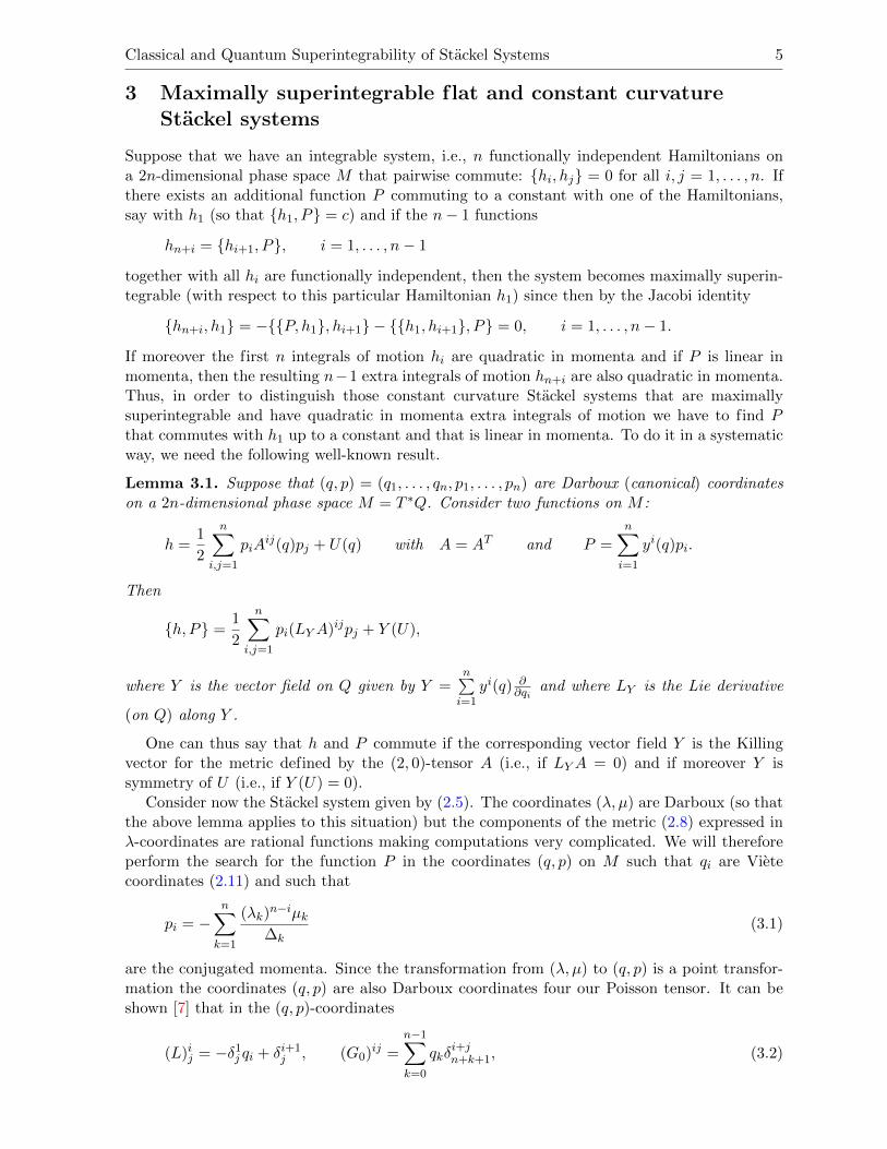
3 Maximally superintegrable flat and constant curvatureStackel systems

Suppose that we have an integrable system, i.e., n functionally independent Hamiltonians ona 2n-dimensional phase space M that pairwise commute: {hi, hj} = 0 for all i, j = 1, . . . , n. Ifthere exists an additional function P commuting to a constant with one of the Hamiltonians,say with h1 (so that {h1, P} = c) and if the n− 1 functions

hn+i = {hi+1, P}, i = 1, . . . , n− 1

together with all hi are functionally independent, then the system becomes maximally superin-tegrable (with respect to this particular Hamiltonian h1) since then by the Jacobi identity

{hn+i, h1} = −{{P, h1}, hi+1} − {{h1, hi+1}, P} = 0, i = 1, . . . , n− 1.

If moreover the first n integrals of motion hi are quadratic in momenta and if P is linear inmomenta, then the resulting n−1 extra integrals of motion hn+i are also quadratic in momenta.Thus, in order to distinguish those constant curvature Stackel systems that are maximallysuperintegrable and have quadratic in momenta extra integrals of motion we have to find Pthat commutes with h1 up to a constant and that is linear in momenta. To do it in a systematicway, we need the following well-known result.

Lemma 3.1. Suppose that (q, p) = (q1, . . . , qn, p1, . . . , pn) are Darboux (canonical) coordinateson a 2n-dimensional phase space M = T ∗Q. Consider two functions on M :

h =1

2

n∑i,j=1

piAij(q)pj + U(q) with A = AT and P =

n∑i=1

yi(q)pi.

Then

{h, P} =1

2

n∑i,j=1

pi(LYA)ijpj + Y (U),

where Y is the vector field on Q given by Y =n∑i=1

yi(q) ∂∂qi

and where LY is the Lie derivative

(on Q) along Y .

One can thus say that h and P commute if the corresponding vector field Y is the Killingvector for the metric defined by the (2, 0)-tensor A (i.e., if LYA = 0) and if moreover Y issymmetry of U (i.e., if Y (U) = 0).

Consider now the Stackel system given by (2.5). The coordinates (λ, µ) are Darboux (so thatthe above lemma applies to this situation) but the components of the metric (2.8) expressed inλ-coordinates are rational functions making computations very complicated. We will thereforeperform the search for the function P in the coordinates (q, p) on M such that qi are Vietecoordinates (2.11) and such that

pi = −n∑k=1

(λk)n−iµk

∆k(3.1)

are the conjugated momenta. Since the transformation from (λ, µ) to (q, p) is a point transfor-mation the coordinates (q, p) are also Darboux coordinates four our Poisson tensor. It can beshown [7] that in the (q, p)-coordinates

(L)ij = −δ1j qi + δi+1

j , (G0)ij =

n−1∑k=0

qkδi+jn+k+1, (3.2)

6 M. B laszak and K. Marciniak

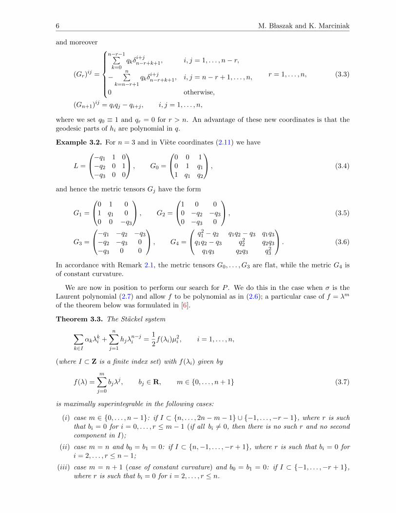
and moreover

(Gr)ij =

n−r−1∑k=0

qkδi+jn−r+k+1, i, j = 1, . . . , n− r,

−n∑

k=n−r+1

qkδi+jn−r+k+1, i, j = n− r + 1, . . . , n,

0 otherwise,

r = 1, . . . , n, (3.3)

(Gn+1)ij = qiqj − qi+j , i, j = 1, . . . , n,

where we set q0 ≡ 1 and qr = 0 for r > n. An advantage of these new coordinates is that thegeodesic parts of hi are polynomial in q.

Example 3.2. For n = 3 and in Viete coordinates (2.11) we have

L =

−q1 1 0−q2 0 1−q3 0 0

, G0 =

0 0 10 1 q1

1 q1 q2

, (3.4)

and hence the metric tensors Gj have the form

G1 =

0 1 01 q1 00 0 −q3

, G2 =

1 0 00 −q2 −q3

0 −q3 0

, (3.5)

G3 =

−q1 −q2 −q3

−q2 −q3 0−q3 0 0

, G4 =

q21 − q2 q1q2 − q3 q1q3

q1q2 − q3 q22 q2q3

q1q3 q2q3 q23

. (3.6)

In accordance with Remark 2.1, the metric tensors G0, . . . , G3 are flat, while the metric G4 isof constant curvature.

We are now in position to perform our search for P . We do this in the case when σ is theLaurent polynomial (2.7) and allow f to be polynomial as in (2.6); a particular case of f = λm

of the theorem below was formulated in [6].

Theorem 3.3. The Stackel system

∑k∈I

αkλki +

n∑j=1

hjλn−ji =

1

2f(λi)µ

2i , i = 1, . . . , n,

(where I ⊂ Z is a finite index set) with f(λi) given by

f(λ) =m∑j=0

bjλj , bj ∈ R, m ∈ {0, . . . , n+ 1} (3.7)

is maximally superintegrable in the following cases:

(i) case m ∈ {0, . . . , n − 1}: if I ⊂ {n, . . . , 2n −m − 1} ∪ {−1, . . . ,−r − 1}, where r is suchthat bi = 0 for i = 0, . . . , r ≤ m − 1 (if all bi 6= 0, then there is no such r and no secondcomponent in I);

(ii) case m = n and b0 = b1 = 0: if I ⊂ {n,−1, . . . ,−r + 1}, where r is such that bi = 0 fori = 2, . . . , r ≤ n− 1;

(iii) case m = n + 1 (case of constant curvature) and b0 = b1 = 0: if I ⊂ {−1, . . . ,−r + 1},where r is such that bi = 0 for i = 2, . . . , r ≤ n.

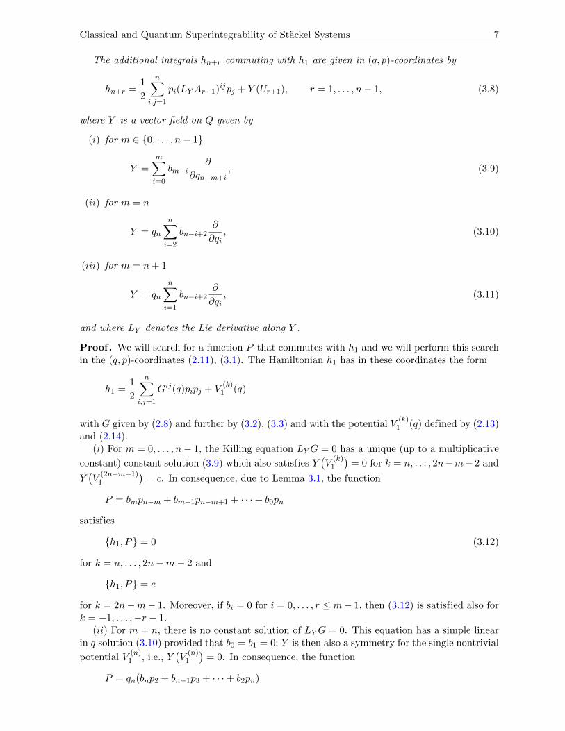
Classical and Quantum Superintegrability of Stackel Systems 7

The additional integrals hn+r commuting with h1 are given in (q, p)-coordinates by

hn+r =1

2

n∑i,j=1

pi(LYAr+1)ijpj + Y (Ur+1), r = 1, . . . , n− 1, (3.8)

where Y is a vector field on Q given by

(i) for m ∈ {0, . . . , n− 1}

Y =

m∑i=0

bm−i∂

∂qn−m+i, (3.9)

(ii) for m = n

Y = qn

n∑i=2

bn−i+2∂

∂qi, (3.10)

(iii) for m = n+ 1

Y = qn

n∑i=1

bn−i+2∂

∂qi, (3.11)

and where LY denotes the Lie derivative along Y .

Proof. We will search for a function P that commutes with h1 and we will perform this searchin the (q, p)-coordinates (2.11), (3.1). The Hamiltonian h1 has in these coordinates the form

h1 =1

2

n∑i,j=1

Gij(q)pipj + V(k)

1 (q)

with G given by (2.8) and further by (3.2), (3.3) and with the potential V(k)

1 (q) defined by (2.13)and (2.14).

(i) For m = 0, . . . , n− 1, the Killing equation LYG = 0 has a unique (up to a multiplicative

constant) constant solution (3.9) which also satisfies Y(V

(k)1

)= 0 for k = n, . . . , 2n−m− 2 and

Y(V

(2n−m−1)1

)= c. In consequence, due to Lemma 3.1, the function

P = bmpn−m + bm−1pn−m+1 + · · ·+ b0pn

satisfies

{h1, P} = 0 (3.12)

for k = n, . . . , 2n−m− 2 and

{h1, P} = c

for k = 2n−m− 1. Moreover, if bi = 0 for i = 0, . . . , r ≤ m− 1, then (3.12) is satisfied also fork = −1, . . . ,−r − 1.

(ii) For m = n, there is no constant solution of LYG = 0. This equation has a simple linearin q solution (3.10) provided that b0 = b1 = 0; Y is then also a symmetry for the single nontrivial

potential V(n)

1 , i.e., Y(V

(n)1

)= 0. In consequence, the function

P = qn(bnp2 + bn−1p3 + · · ·+ b2pn)

8 M. B laszak and K. Marciniak

satisfies (3.12). Moreover, if bi = 0 for i = 2, . . . , r ≤ n − 1 then (3.12) is satisfied also fork = −1, . . . ,−r + 1.

(iii) For m = n + 1 there is no constant solution of LYG = 0. This equation has a simplelinear in q solution (3.11) provided that b0 = b1 = 0 but Y is not a symmetry for any nontrivial

potential V(k)

1 . In consequence, the function

P = qn(bn+1p1 + bnp2 + · · ·+ b2pn).

Poisson commutes only with the geodesic part E1 of h1: {E1, P} = 0. However, if bi = 0 fori = 2, . . . , r ≤ n then (3.12) is satisfied for k = −1, . . . ,−r + 1.

Finally, the form of additional integrals hn+r in (3.8) is obtained through hn+r = {hr+1, P}by using Lemma 3.1. Due to their form, the functions h1, . . . , h2n−1 are functionally indepen-dent. �

Remark 3.4. The above theorem provides us with a sufficient condition for maximal super-integrability of Stackel systems of constant curvature (flat in particular) in case when f(λ) isa polynomial of maximal order n + 1. In consequence, the case (i) of Theorem 3.3 yields an(n+ 1)-parameter family of maximally superintegrable systems, parametrized by

{br, . . . , bm, α−r−1, . . . , α−1, αn, . . . , α2n−m−1}, r = 0, . . . ,m,

where bj parametrize superintegrable metrics (2.6), (2.8) and αj parametrize families of non-trivial superintegrable potentials U (2.12) (in case there is no r, i.e., all bi 6= 0) then there isno α−j in the above set. Similarly, in the cases (ii) and (iii) Theorem 3.3 yields appropriaten-parameter families of superintegrable systems. A particular case of that classification (for themonomial case f(λ) = λm) was presented in [21].

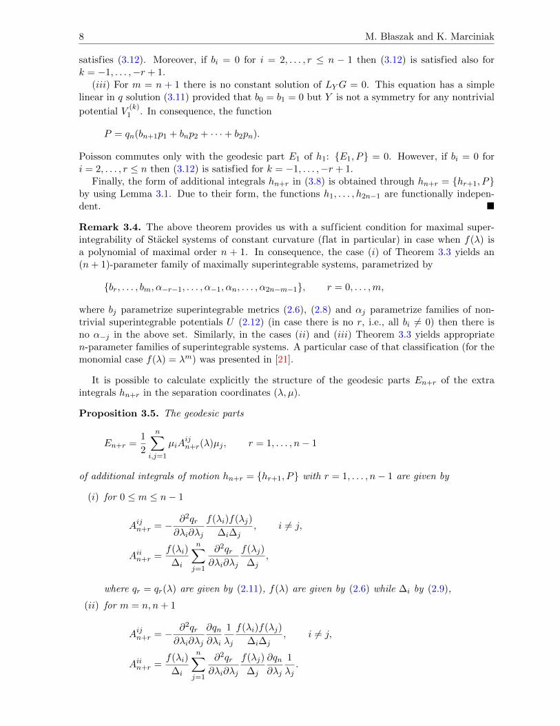
It is possible to calculate explicitly the structure of the geodesic parts En+r of the extraintegrals hn+r in the separation coordinates (λ, µ).

Proposition 3.5. The geodesic parts

En+r =1

2

n∑i,j=1

µiAijn+r(λ)µj , r = 1, . . . , n− 1

of additional integrals of motion hn+r = {hr+1, P} with r = 1, . . . , n− 1 are given by

(i) for 0 ≤ m ≤ n− 1

Aijn+r = − ∂2qr∂λi∂λj

f(λi)f(λj)

∆i∆j, i 6= j,

Aiin+r =f(λi)

∆i

n∑j=1

∂2qr∂λi∂λj

f(λj)

∆j,

where qr = qr(λ) are given by (2.11), f(λ) are given by (2.6) while ∆i by (2.9),

(ii) for m = n, n+ 1

Aijn+r = − ∂2qr∂λi∂λj

∂qn∂λi

1

λj

f(λi)f(λj)

∆i∆j, i 6= j,

Aiin+r =f(λi)

∆i

n∑j=1

∂2qr∂λi∂λj

f(λj)

∆j

∂qn∂λj

1

λj.

Classical and Quantum Superintegrability of Stackel Systems 9

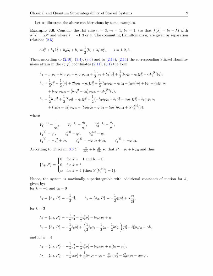
Let us illustrate the above considerations by some examples.

Example 3.6. Consider the flat case n = 3, m = 1, b1 = 1, (so that f(λ) = b0 + λ) withσ(λ) = αλk and where k = −1, 3 or 4. The commuting Hamiltonians hi are given by separationrelations (2.5)

αλki + h1λ2i + h2λi + h3 =

1

2(b0 + λi)µ

2i , i = 1, 2, 3.

Then, according to (2.10), (3.4), (3.6) and to (2.13), (2.14) the corresponding Stackel Hamilto-nians attain in the (q, p) coordinates (2.11), (3.1) the form

h1 = p1p2 + b0p1p3 + b0q1p2p3 +1

2(q1 + b0)p2

2 +1

2(b0q2 − q3)p2

3 + αV(k)

1 (q),

h2 =1

2p2

1 +1

2

(q2

1 + 2b0q1 − q2

)p2

2 +1

2(b0q1q2 − q1q3 − b0q3)p2

3 + (q1 + b0)p1p2

+ b0q1p1p3 +(b0q

21 − q3

)p2p3 + αV

(k)2 (q),

h3 =1

2b0p

21 +

1

2(b0q

21 − q3)p2

2 +1

2

(−b0q1q3 + b0q

22 − q2q3

)p2

3 + b0q1p1p2

+ (b0q2 − q3)p1p3 + (b0q1q2 − q1q3 − b0q3)p2p3 + αV(k)

3 (q),

where

V(−1)

1 =1

q3, V

(−1)2 =

q1

q3, V

(−1)3 =

q2

q3,

V(3)

1 = q1, V(3)

2 = q2, V(3)

3 = q3,

V(4)

1 = −q21 + q2, V

(4)2 = −q1q2 + q3, V

(4)3 = −q1q3.

According to Theorem 3.3 Y = ∂∂q2

+ b0∂∂q3

so that P = p2 + b0p3 and thus

{h1, P} =

0 for k = −1 and b0 = 0,

0 for k = 3,

α for k = 4(then Y

(V

(4)1

)= 1).

Hence, the system is maximally superintegrable with additional constants of motion for h1

given by:for k = −1 and b0 = 0

h4 = {h2, P} = −1

2p2

2, h5 = {h3, P} = −1

2q3p

23 + α

q3

q23

,

for k = 3

h4 = {h2, P} = −1

2p2

2 −1

2b20p

23 − b0p2p3 + α,

h5 = {h3, P} = −1

2b0p

22 +

(1

2b0q2 −

1

2q3 −

1

2b20q1

)p2

3 − b20p2p3 + αb0,

and for k = 4

h4 = {h2, P} = −1

2p2

2 −1

2b20p

23 − b0p2p3 + α(b0 − q1),

h5 = {h3, P} = −1

2b0p

22 +

1

2(b0q2 − q3 − b20q1)p2

3 − b20p2p3 − αb0q1.

10 M. B laszak and K. Marciniak

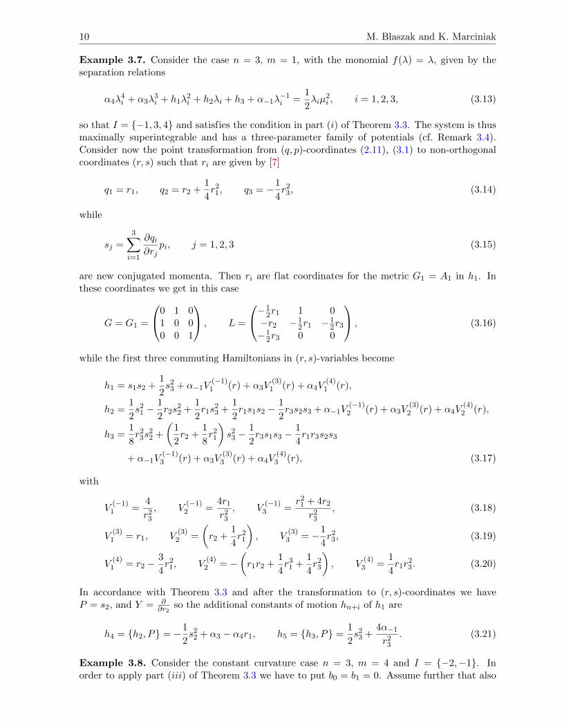
Example 3.7. Consider the case n = 3, m = 1, with the monomial f(λ) = λ, given by theseparation relations

α4λ4i + α3λ

3i + h1λ

2i + h2λi + h3 + α−1λ

−1i =

1

2λiµ

2i , i = 1, 2, 3, (3.13)

so that I = {−1, 3, 4} and satisfies the condition in part (i) of Theorem 3.3. The system is thusmaximally superintegrable and has a three-parameter family of potentials (cf. Remark 3.4).Consider now the point transformation from (q, p)-coordinates (2.11), (3.1) to non-orthogonalcoordinates (r, s) such that ri are given by [7]

q1 = r1, q2 = r2 +1

4r2

1, q3 = −1

4r2

3, (3.14)

while

sj =3∑i=1

∂qi∂rj

pi, j = 1, 2, 3 (3.15)

are new conjugated momenta. Then ri are flat coordinates for the metric G1 = A1 in h1. Inthese coordinates we get in this case

G = G1 =

0 1 01 0 00 0 1

, L =

−12r1 1 0−r2 −1

2r1 −12r3

−12r3 0 0

, (3.16)

while the first three commuting Hamiltonians in (r, s)-variables become

h1 = s1s2 +1

2s2

3 + α−1V(−1)

1 (r) + α3V(3)

1 (r) + α4V(4)

1 (r),

h2 =1

2s2

1 −1

2r2s

22 +

1

2r1s

23 +

1

2r1s1s2 −

1

2r3s2s3 + α−1V

(−1)2 (r) + α3V

(3)2 (r) + α4V

(4)2 (r),

h3 =1

8r2

3s22 +

(1

2r2 +

1

8r2

1

)s2

3 −1

2r3s1s3 −

1

4r1r3s2s3

+ α−1V(−1)

3 (r) + α3V(3)

3 (r) + α4V(4)

3 (r), (3.17)

with

V(−1)

1 =4

r23

, V(−1)

2 =4r1

r23

, V(−1)

3 =r2

1 + 4r2

r23

, (3.18)

V(3)

1 = r1, V(3)

2 =

(r2 +

1

4r2

1

), V

(3)3 = −1

4r2

3, (3.19)

V(4)

1 = r2 −3

4r2

1, V(4)

2 = −(r1r2 +

1

4r3

1 +1

4r2

3

), V

(4)3 =

1

4r1r

23. (3.20)

In accordance with Theorem 3.3 and after the transformation to (r, s)-coordinates we haveP = s2, and Y = ∂

∂r2so the additional constants of motion hn+i of h1 are

h4 = {h2, P} = −1

2s2

2 + α3 − α4r1, h5 = {h3, P} =1

2s2

3 +4α−1

r23

. (3.21)

Example 3.8. Consider the constant curvature case n = 3, m = 4 and I = {−2,−1}. Inorder to apply part (iii) of Theorem 3.3 we have to put b0 = b1 = 0. Assume further that also

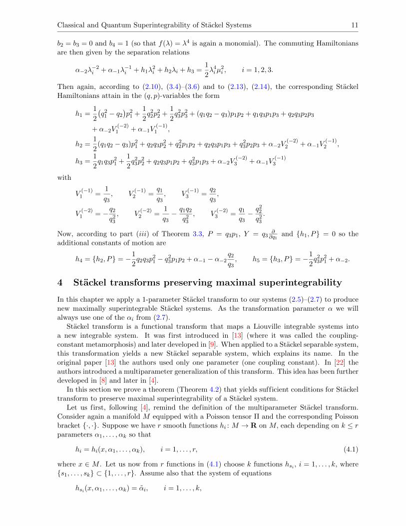
Classical and Quantum Superintegrability of Stackel Systems 11

b2 = b3 = 0 and b4 = 1 (so that f(λ) = λ4 is again a monomial). The commuting Hamiltoniansare then given by the separation relations

α−2λ−2i + α−1λ

−1i + h1λ

2i + h2λi + h3 =

1

2λ4iµ

2i , i = 1, 2, 3.

Then again, according to (2.10), (3.4)–(3.6) and to (2.13), (2.14), the corresponding StackelHamiltonians attain in the (q, p)-variables the form

h1 =1

2

(q2

1 − q2

)p2

1 +1

2q2

2p22 +

1

2q2

3p23 + (q1q2 − q3)p1p2 + q1q3p1p3 + q2q3p2p3

+ α−2V(−2)

1 + α−1V(−1)

1 ,

h2 =1

2(q1q2 − q3)p2

1 + q2q3p22 + q2

2p1p2 + q2q3p1p3 + q23p2p3 + α−2V

(−2)2 + α−1V

(−1)2 ,

h3 =1

2q1q3p

21 +

1

2q2

3p22 + q2q3p1p2 + q2

3p1p3 + α−2V(−2)

3 + α−1V(−1)

3

with

V(−1)

1 =1

q3, V

(−1)2 =

q1

q3, V

(−1)3 =

q2

q3,

V(−2)

1 = −q2

q23

, V(−2)

2 =1

q3− q1q2

q23

, V(−2)

3 =q1

q3− q2

2

q23

.

Now, according to part (iii) of Theorem 3.3, P = q3p1, Y = q3∂∂q1

and {h1, P} = 0 so theadditional constants of motion are

h4 = {h2, P} = −1

2q2q3p

21 − q2

3p1p2 + α−1 − α−2q2

q3, h5 = {h3, P} = −1

2q2

3p21 + α−2.

4 Stackel transforms preserving maximal superintegrability

In this chapter we apply a 1-parameter Stackel transform to our systems (2.5)–(2.7) to producenew maximally superintegrable Stackel systems. As the transformation parameter α we willalways use one of the αi from (2.7).

Stackel transform is a functional transform that maps a Liouville integrable systems intoa new integrable system. It was first introduced in [13] (where it was called the coupling-constant metamorphosis) and later developed in [9]. When applied to a Stackel separable system,this transformation yields a new Stackel separable system, which explains its name. In theoriginal paper [13] the authors used only one parameter (one coupling constant). In [22] theauthors introduced a multiparameter generalization of this transform. This idea has been furtherdeveloped in [8] and later in [4].

In this section we prove a theorem (Theorem 4.2) that yields sufficient conditions for Stackeltransform to preserve maximal superintegrability of a Stackel system.

Let us first, following [4], remind the definition of the multiparameter Stackel transform.Consider again a manifold M equipped with a Poisson tensor Π and the corresponding Poissonbracket {·, ·}. Suppose we have r smooth functions hi : M → R on M, each depending on k ≤ rparameters α1, . . . , αk so that

hi = hi(x, α1, . . . , αk), i = 1, . . . , r, (4.1)

where x ∈ M . Let us now from r functions in (4.1) choose k functions hsi , i = 1, . . . , k, where{s1, . . . , sk} ⊂ {1, . . . , r}. Assume also that the system of equations

hsi(x, α1, . . . , αk) = αi, i = 1, . . . , k,

12 M. B laszak and K. Marciniak

(where αi is another set of k free parameters, or values of Hamiltonians hsi) involving thefunctions hsi can be solved for the parameters αi yielding

αi = hsi(x, α1, . . . , αk), i = 1, . . . , k, (4.2)

where the right hand sides of these solutions define k new functions hsi on M , each dependingon k parameters αi. Finally, let us define r− k functions hi for i = 1, . . . , r, i /∈ {s1, . . . , sk}, bysubstituting hsi from (4.2) instead of αi in hi:

hi = hi|α1→hs1 ,...,αk→hsk, i = 1, . . . , r, i /∈ {s1, . . . , sk}. (4.3)

Definition 4.1. The functions hi = hi(x, α1, . . . , αk), i = 1, . . . , r, defined through (4.2)and (4.3) are called the (generalized) Stackel transform of the functions (4.1) with respect tothe indices {s1, . . . , sk} (or with respect to the functions hs1 , . . . , hsk).

Unless we extend the manifold M this operation cannot be obtained by any coordinatechange of variables. Moreover, if we perform again the Stackel transform on the functions hiwith respect to hsi we will receive back the functions hi in (4.1). In this sense the Stackeltransform is a reciprocal transform. Note also that neither r nor k are related to the dimensionof the manifold M .

In [4] we proved that if dimM = 2n, k = r = n and if all hi are functionally independent thenalso all hi will be functionally independent and if all hi are pairwise in involution with respectto Π then also all hi will pairwise Poisson-commute. That means that if the functions hi,i = 1, . . . , n constitute a Liouville integrable system then also hi will constitute a Liouvilleintegrable system. In other words, Stackel transform preserves Liouville integrability. But whatabout superintegrability?

Theorem 4.2. Consider a maximally superintegrable system on a 2n-dimensional Poissonmanifold, i.e., a set of 2n − 1 functionally independent Hamiltonians h1, . . . , h2n−1 such thatthe first n Hamiltonians pairwise commute, and assume that all the Hamiltonians depend onk ≤ n parameters αi:

hi = hi(x, α1, . . . , αk), i = 1, . . . , 2n− 1,

{hi, hj} = 0, i, j = 1, . . . , n, for all αi, (4.4)

{h1, hn+j} = 0, j = 1, . . . , n− 1, for all αi.

Suppose that {s1, . . . , sk} ⊂ {1, . . . , 2n − 1} are chosen so that s1 = 1 and that {s2, . . . , sk}⊂ {2, . . . , n} and moreover that h1 = h1(x, α1). Then the Stackel transform hi, i = 1, . . . ,2n−1 given by (4.2), (4.3) also satisfy (4.4) and therefore constitute a maximally superintegrablesystem.

Note that the Hamiltonian h1 is now distinguished as the one that commutes with all theremaining hi and as it can only depend on one parameter. Note also that the first n functions hipairwise commute with each other and therefore constitute a Liouville integrable system. Thesame is true about the first n functions hi.

Proof. Differentiating the identity

hsi(x, hs1(x, α1, . . . , αk), . . . , hsk(x, α1, . . . , αk)

)= αi, i = 1, . . . , k

with respect to x we get

dhsi = −k∑j=1

∂hsi∂αj

dhsj , i = 1, . . . , k, (4.5)

Classical and Quantum Superintegrability of Stackel Systems 13

while differentiation of (4.3) yields

dhi = dhi −k∑j=1

∂hi∂αj

dhsj , i = 1, . . . , 2n− 1, i /∈ {s1, . . . , sk}. (4.6)

The transformation (4.5), (4.6) can be written in a matrix form as

dh = Adh,

where we denote dh = (dh1, . . . , dh2n−1)T and dh = (dh1, . . . , dh2n−1)T and where the (2n− 1)×(2n− 1) matrix A has the form

Aij = δij for j /∈ {s1, . . . , sk}, Aisj = − ∂hi∂αj

for j = 1, . . . , k.

Since

detA = ±det

(∂hsi∂αj

)is not zero and since hi are by assumption functionally independent on M we conclude thatalso the functions hi are functionally independent on M . Further, since sk ≤ n (the Stackeltransform is taken with respect to the Hamiltonians belonging to the Liouville integrable systemh1, . . . , hn) the columns with derivatives of hi with respect to parameters αj all lie in the lefthand side of the matrix A. Moreover, the fact that h1 = h1(x, α1) also means that the first rowof A is zero except A11 = − ∂hi

∂α1. Let us now introduce the (2n− 1)× (2n− 1) matrices C and D

through Cij = {hi, hj} and Dij = {hi, hj}. A direct calculation yields

{hi, hj

}=

2n−1∑l1,l2=1

(A−1

)il1

(A−1

)jl2{hl1 , hl2}Π

or in matrix form

D = A−1C(A−1

)T,

and due to the aforementioned structure of A we have Dij = 0 for i, j = 1, . . . , n (meaningthat h1, . . . , hn constitute a Liouville integrable system) and moreover that D1i = Di1 = 0 fori = 1, . . . , 2n− 1, so that {h1, hi} = 0 for all i. That concludes the proof. �

Remark 4.3. A similar statement with an analogous proof is valid for any superintegrablesystem of the form (4.4), not only the maximally superintegrable one.

5 Stackel transform of maximally superintegrableStackel systems

In this section we perform those Stackel transforms of our systems (2.5)–(2.7) that preservemaximal superintegrability. According to Theorem 4.2, the Hamiltonian h1 of the consideredsystem can only depend on one parameter h1 = h1(x, α). It is then natural to choose one ofthe ak in (2.7) as this parameter.

Consider thus a maximally superintegrable system (h1, . . . , h2n−1) with the first n commutingHamiltonians h1, . . . , hn defined by our separation relations∑

s∈Iαsλ

si + h1λ

n−1i + h2λ

n−2i + · · ·+ hn =

1

2f(λi)µ

2i , i = 1, . . . , n,

14 M. B laszak and K. Marciniak

where the index set I satisfies the assumptions of Theorem 3.3 and where the higher integralshn+r are constructed as usual through hn+r = {hr+1, P} with P constructed as in Theorem 3.3.Let us now choose one of the parameters αs, with s ∈ I, say αk, (we will suppose that k ≥ nor k < 0 otherwise the corresponding potential is trivial, as explained earlier) and define thefunctions Hr, r = 1, . . . , 2n− 1, through

hr = Hr + αkV(k)r , r = 1, . . . , 2n− 1. (5.1)

Then V(k)r for r = 1, . . . , n obviously coincide with V

(k)r defined through (2.5)–(2.7) or equiva-

lently through (2.13), (2.14).We now perform the Stackel transform on this system (h1, . . . , h2n−1) with respect to the

chosen parameter αk as described in Theorem 4.2. It means that we first solve the relation

h1 = α, i.e., H1 + αkV(k)

1 = α with respect to αk which yields

h1 = αk = − 1

V(k)

1

H1 + α1

V(k)

1

, (5.2)

and then replace αk with h1 in all the remaining Hamiltonians:

hr = Hr −V

(k)r

V(k)

1

H1 + αV

(k)r

V(k)

1

, r = 2, . . . , 2n− 1. (5.3)

We obtain in this way a new superintegrable system (h1, . . . , h2n−1) where the first n commutingHamiltonians hr are defined by (see [4]) the following separation relations

h1λki +

∑s∈I, s 6=k

αsλsi + αλn−1

i + h2λn−2i + · · ·+ hn =

1

2f(λi)µ

2i , i = 1, . . . , n, (5.4)

as it is easy to see, since on the level of the separation relations our Stackel transform replaces αkwith h1 and h1 with α. For k ≥ n or k < −1 the system (5.4) is no longer in the class (2.5),while for k = −1 it can be easily transformed by a simple point transformation to the form (2.5).

Lemma 5.1. The separable system

αkλki +

∑s∈I, s 6=k

αsλsi + h1λ

n−1i + h2λ

n−2i + · · ·+ hn =

1

2λmi µ

2i , i = 1, . . . , n

attains after the Stackel transform (5.2), (5.3) and after the consecutive point transformationon M given by

λi → 1/λi, µi → −λ2iµi, i = 1, . . . , n (5.5)

the form

αλ−1i +

∑s∈I, s 6=k

αsλn−2−si + h1λ

n−k−2i + hnλ

n−2i + · · ·+ h2

=1

2λn−m+2i µ2

i , i = 1, . . . , n. (5.6)

Note that the transformation (5.5) on M does not change the separation web of the systemon Q. Denoting, as before

hr = Hr + αVr, r = 1, . . . , 2n− 1, (5.7)

Classical and Quantum Superintegrability of Stackel Systems 15

where hr for r = 1, . . . , n are defined by (5.4) while hr for r = n+ 1, . . . , 2n− 1 are obtained asusual through hn+r =

{hr+1, P

}, we see from (5.3) that

Vr = Vr −V

(k)r

V(k)

1

V1, r = 2, . . . , 2n− 1,

and from (5.2) it also follows that the geodesic part E1 of h1 has the form

E1 =n∑

i,j=1

Gijpipj , G = − 1

V(k)

1

G. (5.8)

It means that the metric G is a conformal deformation of either a flat or a constant curvaturemetric G. In the following theorem we list the cases when the metric G is actually flat or ofconstant curvature as well. The theorem is formulated only for f in (2.6) being a monomial,f = λm (in this case there is a maximum number of flat metrics G).

Theorem 5.2. Consider the system (5.4) with f = λm where m ∈ {0, . . . , n+ 1}.

(i) For 0 ≤ m ≤ n− 1 the system (5.4) is maximally superintegrable for k ∈ {−m, . . . ,−1, n,. . . , 2n −m − 1}. The metric G in (5.8) is flat for k ∈ {−[m/2], . . . ,−1, n, . . . , n − 1 +[(n−m)/2]}, where [·] denotes the integer part. Moreover, for m = 1 and k = −1 G is ofconstant curvature. Otherwise G is conformally flat.

(ii) For m = n the system (5.4) is maximally superintegrable for k ∈ {−(n − 2), . . . ,−1, n}.The metric G in (5.8) is flat for k ∈ {−[n/2], . . . ,−1}. Otherwise G is conformally flat.

(iii) For m = n+ 1 the system (5.4) is maximally superintegrable for k ∈ {−(n− 1), . . . ,−1}.The metric G in (5.8) is flat for k ∈ {−[(n+ 1)/2], . . . ,−1}. Otherwise G is conformallyflat.

If f is a polynomial then the admissible values of k must satisfy the above type of bonds forall powers of λ in f , not only for the highest power m so we choose not to present this moregeneral theorem, only to maintain the simplicity of the picture. In order to prove Theorem 5.2we need one more lemma.

Lemma 5.3 ([20]). The Ricci scalars R and R of the conformally related (covariant) metrictensors g and g = σg are related through

R = σ−1R− 1

2(n− 1)σ−1sijG

ij , (5.9)

where G = g−1 and where

sij = sji = 2∇isj − sisj +1

2gijsks

k with si = σ−1 ∂σ

∂xi,

where xi are any coordinates on the manifold.

Proof of Theorem 5.2. The values of k for which (5.1) is maximally superintegrable followsfrom the specification of Theorem 3.3 to the case f = λm. For (i) and (ii) the metric G in (5.8) isflat so that its Ricci scalar R = 0. Therefore, according to (5.9), R = 0 if and only if sijG

ij = 0.This condition can be effectively calculated in flat coordinates ri of the metric G given by [7]

qi = ri +1

4

i−1∑j=1

rjri−j , i = 1, . . . , n−m,

qi = −1

4

n∑j=i

rjrn−j+i, i = n−m+ 1, . . . ,m.

16 M. B laszak and K. Marciniak

In these coordinates

(Gm)kl = δk+ln−m+1 + δk+l

2n−m+1

and the condition sijGij = 0 yields both statements. The case in (i) when G is of constant

curvature (m = 1, k = −1) can be however more effectively proven using Lemma 5.1 since inthis case the system (5.4) attains after the transformation (5.5) the form

h1λn−1i +

∑s∈I, s 6=k

αsλn−2−si + hnλ

n−2i + · · ·+ h2 + αλ−1

i =1

2λn+1i µ2

i , i = 1, . . . , n.

Due to Remark 2.1 the metric G of this system has constant curvature. Finally, in the case (iii)(m = n+ 1) we have only negative potentials so by using Lemma 5.1 we transform this systemto

h1λn−k−2i +

∑s∈I, s 6=k

αsλn−2−si + hnλ

n−2i + · · ·+ h2 + αλ−1

i =1

2λiµ

2i , i = 1, . . . , n,

where k < 0, and this is the system from case (i) with m = 1 and therefore G is flat fork ≥ −[(n+ 1)/2]. For other values of k the metric G is conformally flat. �

If Y (V(k)

1 ) = 0 then Y (1/V(k)

1 ) = 0 and due to (5.8) also LY G = 0 so that {h1, P} = 0 aswell and the same P as in the “non-tilde”-case (i.e., before the Stackel transform) can be usedas an alternative definition of extra Hamiltonians through hn+r = {hr+1, P}, r = 1, . . . , n − 1.

This is however no longer true if Y(V

(k)1

)= c 6= 0 (according to Theorem 3.3, it happens only in

the case when m < n and k = 2n−m− 1). It turns out that it leads to the same extra integralsof motion, as the following theorem states

Theorem 5.4. If Y (V(k)

1 ) = 0 then both sets of extra integrals of motion:

hn+r = {hr+1, P}, r = 1, . . . , n− 1

and

hn+r = hn+r|α=h1(α), r = 1, . . . , n− 1

coincide.

Proof. On one hand, according to (5.3) and due to the fact that {h1, P} = 0 we have

hn+r ={hr+1, P

}=

{Hr+1 −

V(k)r+1

V(k)

1

H1 + αV

(k)r+1

V(k)

1

, P

}

= {Hr+1, P} −H1

V(k)

1

{V

(k)r+1, P

}+

α

V(k)

1

{V

(k)r+1, P

}= {Hr+1, P}+ h1

{V

(k)r+1, P

}.

On the other hand, due to

hn+r = hn+r|α=h1(α)= {hr+1, P}|α=h1(α)

= {Hr+1, P}+ α{V

(k)r+1, P

}∣∣α=h1(α)

,

which yields the same result. �

Classical and Quantum Superintegrability of Stackel Systems 17

Thus, if Y (V(k)

1 ) = 0, the diagram below commutes

(h1, . . . , hn)P−→ (h1, . . . , h2n−1) with hn+r = {hr+1, P}

| |Stackel transform Stackel transform

↓ ↓(h1, . . . , hn

) P−→(h1, . . . , h2n−1

)with hn+r =

{hr+1, P

}.

Example 5.5. Let us apply the relations (5.2), (5.3) to perform the Stackel transform on thesystem from Example 3.7. To keep the formulas simple, we assume that all the αs in (2.7) arezero except the transformation parameter αk. Thus, we consider again the system given by theseparation relations

αkλki + h1λ

2i + h2λi + h3 =

1

2λiµ

2i , i = 1, 2, 3

with k = −1, 3 or 4, respectively. Applying Stackel transform to the resulting Hamiltonians(3.17)–(3.21) we obtain a maximally superintegrable system with the separation relations of theform:

h1λki + αλ2

i + h2λi + h3 =1

2λiµ

2i , i = 1, 2, 3. (5.10)

Again we perform our calculations in the (r, s)-variables (3.14), (3.15). Explicitly, we obtain fork = −1

h1 =1

8r2

3s23 +

1

4r2

3s1s2 −1

4αr2

3,

h2 =1

2s2

1 −1

2r2s

22 −

1

2r1s1s2 −

1

2r3s2s3 + αr1,

h3 =1

8r2

3s22 −

(1

4r2

1 + r2

)s1s2 −

1

2r3s1s3 −

1

4r1r3s2s3 +

1

4α(r2

1 + 4r2

),

h4 = −1

2s2

2, h5 = −s1s2 + α, (5.11)

for k = 3

h1 = − 1

r1s1s2 −

1

2

1

r1s2

3 + α1

r1,

h2 =1

2s2

1 +1

4

r21 − 4r2

r1s1s2 −

1

2r2s

22 −

1

2r3s2s3 +

1

8

3r21 − 4r2

r1s2

3 +1

4αr2

1 + 4r2

r1,

h3 =1

4

r23

r1s1s2 −

1

2r3s1s3 +

1

8r2

3s22 −

1

4r1r3s2s3 +

1

8

r31 + 4r1r2 + r2

3

r1s2

3 −1

4αr2

3

r1,

h4 = − 1

r1s1s2 −

1

2s2

2 −1

2

1

r1s2

3 + α1

r1, h5 =

1

2s2

3,

and for k = 4

h1 = − 1

r2 − 34r

21

s1s2 −1

2

1

r2 − 34r

21

s23 + α

1

r2 − 34r

21

,

h2 =1

2s2

1 −1

2r2s

22 −

1

8

2r31 − 8r1r2 − r2

3

r2 − 34r

21

s23 −

1

8

r31 − 12r1r2 − 2r2

3

r2 − 34r

21

s1s2 −1

2r3s2s3

− αr1r2 + 1

4r31 + 1

4r23

r2 − 34r

21

,

18 M. B laszak and K. Marciniak

h3 =1

8r2

3s22 −

1

32

3r41 + 8r2

1r2 + 4r1r23 + 16r2

2

r2 − 34r

21

s23 +

1

4

r1r23

r2 − 34r

21

s1s2 −1

2r3s1s3 −

1

4r1r3s2s3

+1

4α

r1r23

r2 − 34r

21

,

h4 = −1

2s2

2 +1

2

r1

r2 − 34r

21

s23 +

r1

r2 − 34r

21

s1s2 − αr1

r2 − 34r

21

, h5 =1

2s2

3. (5.12)

According to part (i) of Theorem 5.2 the metrics of h1 are of constant curvature, flat andconformally flat, respectively.

6 Quantization of maximally superintegrable Stackel systems

This section is devoted to separable quantizations of Stackel systems that were considered inthe classical setting in the previous sections. Let us consider, as in the classical case, an n-dimensional Riemannian space Q equipped with a matric tensor g and the quadratic in momentaHamiltonian on the cotangent bundle T ∗Q:

h =1

2

n∑i,j=1

piAij(x)pj + U(x).

By its minimal quantization [5] we mean the following self-adjoint operator

h = −1

2}2

n∑i,j=1

∇iAij(x)∇j + U(x) = −1

2}2

n∑i,j=1

1√|g|∂i√|g|Aij(x)∂j + U(x) (6.1)

(both expressions on the right hand side of (6.1) are equivalent) acting in the Hilbert space

H = L2(Q, dµ), dµ = |g|1/2dx, |g| = |det g|,

where ∇ is the Levi-Civita connection of the metric g. Note that a priori there is no relationbetween the tensor A and the metric g. Let us now consider an arbitrary Stackel system ofthe form (2.3) coming from the separation relations (2.2). Applying the procedure of minimalquantization to this system will in general yield a non-integrable and non-separable quantumsystem. In order to preserve integrability and separability we have to carefully choose themetric g. To do this, we will use the following theorem, proved in [5].

Theorem 6.1. Suppose that hj are Hamiltonian functions (2.3), defined by separation rela-tions (2.2). Suppose also that θ is an arbitrary function of one variable. Applying to hj theprocedure of minimal quantization (6.1) with the metric tensor

g = ϕ2n gθ, (6.2)

where gθ = G−1θ with Gθ given by

Gθ = diag

(θ(λ1)

∆1, . . . ,

θ(λn)

∆n

), (6.3)

and with ϕ being a particular function of λ1, . . . , λn, uniquely defined by (2.2) (see formula (27)in [5] for details), we obtain a quantum integrable and separable system. More precisely, weobtain n operators hi of the form (6.1) such that (i) [hi, hj ] = 0 for all i, j and (ii) eigenvalue

problems for all hi

hiΨ = εiΨ, i = 1, . . . , n

Classical and Quantum Superintegrability of Stackel Systems 19

have for each choice of eigenvalues εi of hi the common multiplicatively separable eigenfunction

Ψ(λ1, . . . , λn) =n∏i=1

ψ(λi) with ψ satisfying the following ODE (quantum separation relation)(ε1λ

γ1 + ε2λγ2 + · · ·+ εn

)ψ(λ)

= −1

2~2f(λ)

[d2ψ(λ)

dλ2+

(f ′(λ)

f(λ)− 1

2

θ′(λ)

θ(λ)

)dψ(λ)

dλ

]+ σ(λ)ψ(λ). (6.4)

Remark 6.2. For Stackel systems defined by (2.5), when (γ1, . . . , γn) = (n− 1, . . . , 0) in (2.2),we have ϕ = 1 and the most natural choice in (6.3) is to put θ = f which yields the metric forquantization

G = Gf = A1. (6.5)

On the other hand, for Stackel systems defined by (5.4) we have ϕ = −V (k)1 (as it follows

from (5.2) and the formula (27) in [5]) and again the simplest choice in (6.3) is to put θ = fwhich yields according to (6.2) and (5.8) the metric for quantization

G = ϕ−2nGf = ϕ1− 2

n A1. (6.6)

For the choice (6.5) and (6.6) the quantum separation equation (6.4) reduce to(ε1λ

γ1 + ε2λγ2 + · · ·+ εn

)ψ(λ) = −1

2~2f(λ)

[d2ψ(λ)

dλ2+

1

2

f ′(λ)

f(λ)

dψ(λ)

dλ

]+ σ(λ)ψ(λ), (6.7)

where (γ1, . . . , γn) = (n−1, n−2, . . . , 0) in the first case (6.5) and (γ1, . . . , γn) = (k, n−2, n−3,. . . , 0) in the second case (6.6).

Let us now pass to the issue of quantum superintegrability of considered Stackel systems. Weformulate now a quantum analogue of Lemma 3.1.

Lemma 6.3. Suppose that h is given by (6.1) and that Y =n∑i=1

yi(x)∇i is a vector field on the

Riemannian manifold Q with a metric g. Then[h, Y

]=

1

2}2

n∑i,j=1

∇i(LYA)ij∇j +1

2}2

n∑i,j,k=1

Aij(∇j∇kyk

)∇i − Y (U).

One proves this lemma by a direct computation. Thus, a sufficient condition for [h, Y ] = cis satisfied when Y is a Killing vector for both A and g and if moreover U is constant along Y ,that is when

LYA = 0, LY g = 0, Y (U) = c (6.8)

(note that LY g = 0 impliesn∑i=1∇kyk = 0).

Corollary 6.4. Suppose we have a quantum integrable system on the configuration space Q, thatis a set of n commuting and algebraically independent operators h1, . . . , hn of the form (6.1)acting in the Hilbert space L2(Q, |g|1/2dx) where g is some metric on Q. Suppose also thata vector field Y satisfies (6.8) with A1 and U1 instead of A and U (so that [h1, Y ] = c). Then,analogously to the classical case, the operators

hn+r =[hr+1, Y

]=

1

2}2

n∑i,j=1

∇i(LYAr+1)ij∇j − Y (Ur+1), r = 1, . . . , n− 1 (6.9)

satisfy [hn+r, h1] = 0 and the system h1, . . . , h2n−1 is algebraically independent; that is we obtaina quantum separable and quantum superintegrable system.

20 M. B laszak and K. Marciniak

We can now apply this corollary to construct quantum superintegrable counterparts of classi-cal systems considered in previous sections. According to Remark 6.2, for the systems generatedby the separation relations (2.5) the most natural choice of the metric g is to take G = A1 asin (6.5). Then, by construction, [hi, hj ] = 0 for i, j = 1, . . . , n while the remaining operators hn+r

are constructed by the formula (6.9) and are – up to a sign – identical with minimal quantization(in the metric G) of the extra integrals hn+r obtained in (3.8).

Example 6.5. Consider again separation relations (3.13) from Example 3.7, so that f(λ) = λand σ = α−1λ

−1 +α3λ3 +α4λ

4. Performing the minimal quantization of the Hamiltonians (3.17)in the metric G = A1, i.e., given by (3.16), we obtain, in the flat r-coordinates (3.14)

h1 = −1

2}2

(∂1∂2 +

1

2∂2

3

)+ α−1V

(−1)1 (r) + α3V

(3)1 (r) + α4V

(4)1 (r),

h2 = −1

4}2

(∂2

1 − ∂2r2∂2 + r1∂3∂3 +1

2∂1r1∂2 +

1

2r1∂2∂1 − r3

1

2∂2∂3 −

1

2∂3r3∂2

)+ α−1V

(−1)2 (r) + α3V

(3)2 (r) + α4V

(4)2 (r),

h3 = −1

8}2

(1

2r2

3∂22 +

(2r2 +

1

2r2

1

)∂2

3 − r3∂1∂3 − ∂3r3∂1 −1

2r1r3∂2∂3 −

1

2r1∂3r3∂2

)+ α−1V

(−1)3 (r) + α3V

(3)3 (r) + α4V

(4)3 (r),

where ∂i = ∂/∂ri and V(k)i are given by (3.18)–(3.20). The respective separation equation,

according to (3.13) and (6.7), is of the form

(α−1λ

−1 + α3λ3 + α4λ

4 + ε1λ2 + ε2λ+ ε3

)ψ(λ) = −1

2~2

[λd2ψ(λ)

dλ2+

1

2

dψ(λ)

dλ

].

Now Y = ∂2 satisfies the conditions (6.8) and the extra operators h4, h5 can be obtained eitherby using the formula (6.9) or directly by minimal quantization of functions h4, h5 in (3.21). Theresult is (up to a sign)

h4 =1

4}2∂2

2 − α3 + α4r1, h5 = −1

4}2∂2

3 +4α−1

r23

.

If we want to perform the separable quantization of superintegrable systems obtained by theStackel transform, as in Section 5, we have two cases: either the system – after the Stackeltransform – belongs again to the same class (2.5) or belongs to the other class, given by theseparation relations (5.4) that are different from (2.5) as soon as k 6= −1. Again by Remark 6.2,in the first case the natural choice of the metric in which we perform the minimal quantizationis to take G = A1, i.e., G as given by (5.8). In the second case we have to use the metric given

by (6.2) which in our case is given by (6.6), i.e., by G = ϕ1− 2n A1 with ϕ = −V (k)

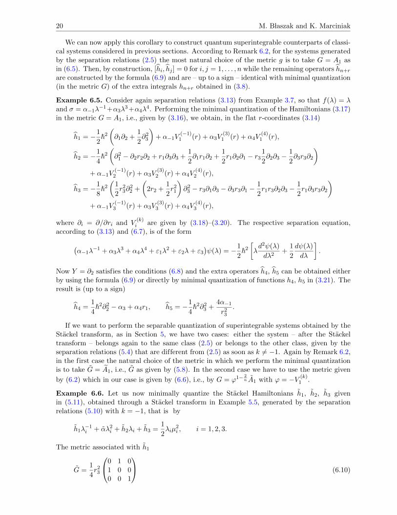
1 .

Example 6.6. Let us now minimally quantize the Stackel Hamiltonians h1, h2, h3 givenin (5.11), obtained through a Stackel transform in Example 5.5, generated by the separationrelations (5.10) with k = −1, that is by

h1λ−1i + αλ2

i + h2λi + h3 =1

2λiµ

2i , i = 1, 2, 3.

The metric associated with h1

G =1

4r2

3

0 1 01 0 00 0 1

(6.10)

Classical and Quantum Superintegrability of Stackel Systems 21

is of constant curvature as – by Lemma 5.1 – after applying transformation (5.5), in the newseparation coordinates the separation relations (5.10) turns to

αλ−1i + h1λ

2i + h3λi + h2 =

1

2λ4iµ

2i , i = 1, 2, 3

and belong again to the class (2.5). Thus, by Remark 6.2, we have to perform the minimal quan-tization of this system with respect to the original metric A1 of the system which is just (6.10).Observing that

√|g| = 8/r3

3, we obtain the following quantum superintegrable system (we usethe second expression in (6.1)):

h1 = −1

4}2r2

3

(1

2r3∂3

1

r3∂3 + ∂1∂2

)− 1

4αr2

3,

h2 =

1

4}2

(−2∂2

1 + 2∂2r2∂2 + ∂1r1∂2 + r1∂2∂1 + r3∂2∂3 + r33∂3

1

r23

∂2

)+ αr1,

h3 =

1

8}2

[−r2

3∂22 + (r2

1 + 4r2)∂1∂2 + ∂1r21∂2 + 4∂2r2∂1 + 2r3∂1∂3 + 2r3

3∂31

r23

∂1

+ r1r3∂2∂3 + r1r33∂3

1

r23

∂1

]+

1

4α(r2

1 + 4r2

),

h4 =

1

2}2∂2

2 ,h5 = }2∂1∂2 + α.

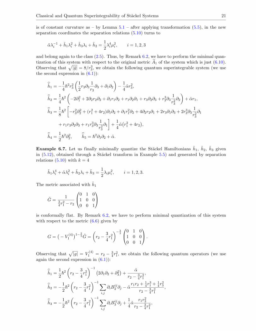
Example 6.7. Let us finally minimally quantize the Stackel Hamiltonians h1, h2, h3 givenin (5.12), obtained through a Stackel transform in Example 5.5) and generated by separationrelations (5.10) with k = 4

h1λ4i + αλ2

i + h2λi + h3 =1

2λiµ

2i , i = 1, 2, 3.

The metric associated with h1

G =1

34r

21 − r2

0 1 01 0 00 0 1

is conformally flat. By Remark 6.2, we have to perform minimal quantization of this systemwith respect to the metric (6.6) given by

G =(− V (4)

1

)1− 23 G =

(r2 −

3

4r2

1

)− 23

0 1 01 0 00 0 1

.

Observing that√|g| = V

(4)1 = r2 − 3

4r21, we obtain the following quantum operators (we use

again the second expression in (6.1)):

h1 =

1

2}2

(r2 −

3

4r2

1

)−1 (2∂1∂2 + ∂2

3

)+

α

r2 − 34r

21

,

h2 = −1

2}2

(r2 −

3

4r2

1

)−1∑i,j

∂iBij2 ∂j − α

r1r2 + 14r

31 + 1

4r23

r2 − 34r

21

,

h3 = −1

2}2

(r2 −

3

4r2

1

)−1∑i,j

∂iBij3 ∂j +

1

4α

r1r23

r2 − 34r

21

,

22 M. B laszak and K. Marciniak

h4 = −1

2}2

(r2 −

3

4r2

1

)−1 [∂1r1∂2 + r1∂2∂1 − ∂2

(r2 −

3

4r2

1

)∂2 + r1∂

23

]− α r1

r2 − 34r

21

,

h5 = −1

2}2∂2

3 ,

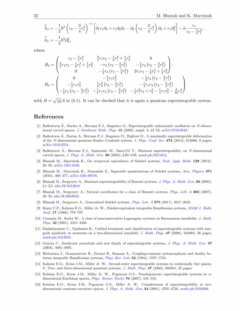
where

B2 =

r2 − 34r

21

32r1r2 − 1

8r31 + 1

4r23 0

32r1r2 − 1

8r31 + 1

4r23 −r2

(r2 − 3

4r21

)−1

2r3

(r2 − 3

4r21

)0 −1

2r3

(r2 − 3

4r21

)2r1r2 − 1

2r31 + 1

4r23

,

B3 =

0 −14r1r

23 −1

2r3

(r2 − 3

4r21

)−1

4r1r23

14r

23

(r2 − 3

4r21

)−1

4r1r3

(r2 − 3

4r21

)−1

2r3

(r2 − 3

4r21

)−1

4r1r3

(r2 − 3

4r21

)−1

2r21r2 + r2

2 − 14r1r

23 − 3

16r41

with B =

√|g|A in (6.1). It can be checked that it is again a quantum superintegrable system.

References

[1] Ballesteros A., Enciso A., Herranz F.J., Ragnisco O., Superintegrable anharmonic oscillators on N -dimen-sional curved spaces, J. Nonlinear Math. Phys. 15 (2008), suppl. 3, 43–52, arXiv:0710.0843.

[2] Ballesteros A., Enciso A., Herranz F.J., Ragnisco O., Riglioni D., A maximally superintegrable deformationof the N -dimensional quantum Kepler–Coulomb system, J. Phys. Conf. Ser. 474 (2013), 012008, 9 pages,arXiv:1310.6554.

[3] Ballesteros A., Herranz F.J., Santander M., Sanz-Gil T., Maximal superintegrability on N -dimensionalcurved spaces, J. Phys. A: Math. Gen. 36 (2003), L93–L99, math-ph/0211012.

[4] B laszak M., Marciniak K., On reciprocal equivalence of Stackel systems, Stud. Appl. Math. 129 (2012),26–50, arXiv:1201.0446.

[5] B laszak M., Marciniak K., Domanski Z., Separable quantizations of Stackel systems, Ann. Physics 371(2016), 460–477, arXiv:1501.00576.

[6] B laszak M., Sergyeyev A., Maximal superintegrability of Benenti systems, J. Phys. A: Math. Gen. 38 (2005),L1–L5, nlin.SI/0412018.

[7] B laszak M., Sergyeyev A., Natural coordinates for a class of Benenti systems, Phys. Lett. A 365 (2007),28–33, nlin.SI/0604022.

[8] B laszak M., Sergyeyev A., Generalized Stackel systems, Phys. Lett. A 375 (2011), 2617–2623.

[9] Boyer C.P., Kalnins E.G., Miller Jr. W., Stackel-equivalent integrable Hamiltonian systems, SIAM J. Math.Anal. 17 (1986), 778–797.

[10] Crampin M., Sarlet W., A class of nonconservative Lagrangian systems on Riemannian manifolds, J. Math.Phys. 42 (2001), 4313–4326.

[11] Daskaloyannis C., Ypsilantis K., Unified treatment and classification of superintegrable systems with inte-grals quadratic in momenta on a two-dimensional manifold, J. Math. Phys. 47 (2006), 042904, 38 pages,math-ph/0412055.

[12] Gonera C., Isochronic potentials and new family of superintegrable systems, J. Phys. A: Math. Gen. 37(2004), 4085–4095.

[13] Hietarinta J., Grammaticos B., Dorizzi B., Ramani A., Coupling-constant metamorphosis and duality be-tween integrable Hamiltonian systems, Phys. Rev. Lett. 53 (1984), 1707–1710.

[14] Kalnins E.G., Kress J.M., Miller Jr. W., Second-order superintegrable systems in conformally flat spaces.V. Two- and three-dimensional quantum systems, J. Math. Phys. 47 (2006), 093501, 25 pages.

[15] Kalnins E.G., Kress J.M., Miller Jr. W., Pogosyan G.S., Nondegenerate superintegrable systems in n-dimensional Euclidean spaces, Phys. Atomic Nuclei 70 (2007), 545–553.

[16] Kalnins E.G., Kress J.M., Pogosyan G.S., Miller Jr. W., Completeness of superintegrability in two-dimensional constant-curvature spaces, J. Phys. A: Math. Gen. 34 (2001), 4705–4720, math-ph/0102006.

Classical and Quantum Superintegrability of Stackel Systems 23

[17] Kalnins E.G., Miller W., Post S., Models for quadratic algebras associated with second order superintegrablesystems in 2D, SIGMA 4 (2008), 008, 21 pages, arXiv:0801.2848.

[18] Marciniak K., B laszak M., Flat coordinates of flat Stackel systems, Appl. Math. Comput. 268 (2015), 706–716, arXiv:1406.2117.

[19] Miller Jr. W., Post S., Winternitz P., Classical and quantum superintegrability with applications, J. Phys. A:Math. Theor. 46 (2013), 423001, 97 pages, arXiv:1309.2694.

[20] Schouten J.A., Ricci-calculus. An introduction to tensor analysis and its geometrical applications,Grundlehren der Mathematischen Wissenschaften, Vol. 10, 2nd ed., Springer-Verlag, Berlin – Gottingen –Heidelberg, 1954.

[21] Sergyeyev A., Exact solvability of superintegrable Benenti systems, J. Math. Phys. 48 (2007), 052114,11 pages, nlin.SI/0701015.

[22] Sergyeyev A., B laszak M., Generalized Stackel transform and reciprocal transformations for finite-dimensional integrable systems, J. Phys. A: Math. Theor. 41 (2008), 105205, 20 pages, arXiv:0706.1473.

[23] Sklyanin E.K., Separation of variables – new trends, Progr. Theoret. Phys. Suppl. (1995), 35–60,solv-int/9504001.

[24] Stackel P., Uber die Integration der Hamilton–Jacobischen Differential Gleichung Mittelst Separation derVariabeln, Habilitationsschrift, Halle, 1891.