arX

iv:c

ond-

mat

/960

7195

v1 2

6 Ju

l 199

6

Two point-contact interferometer for quantum Hall systems

C. de C. ChamonDepartment of Physics, Massachusetts Institute of Technology, Cambridge, MA 02139

D. E. FreedThe Mary Ingraham Bunting Institute, Radcliffe Research and Study Center, Harvard University, Cambridge, MA 02138

S. A. KivelsonDepartment of Physics, University of California at Los Angeles, Los Angeles, California 90095

S. L. SondhiDepartment of Physics, Princeton University, Princeton, NJ 08544

X. G. WenDepartment of Physics, Massachusetts Institute of Technology, Cambridge, MA 02139

We propose a device, consisting of a Hall bar with two weak barriers, that can be used to studyquantum interference effects in a strongly correlated system. We show how the device provides away of measuring the fractional charge and fractional statistics of quasiparticles in the quantumHall effect through an anomalous Aharanov-Bohm period. We discuss how this disentangling ofthe charge and statistics can be accomplished by measurements at fixed filling factor and at fixeddensity. We also discuss a another type of interference effect that occurs in the nonlinear regime asthe source-drain voltage is varied. The period of these oscillations can also be used to measure thefractional charge, and details of the oscillations patterns, in particular the position of the nodes,can be used to distinguish between Fermi-liquid and Luttinger-liquid behavior. We illustrate theseideas by computing the conductance of the device in the framework of edge state theory and use itto estimate parameters for the experimental realization of this device.

PACS: 73.23.-b, 71.10.Pm, 73.40.Hm, 73.40.Gk

I. INTRODUCTION

A considerable amount of work on electronic systems in recent years has focused on two distinct sets of problems:the effects of quantum interference on the behavior of mesoscopic systems and those of strong correlations in lowdimensional systems. Most of the canonical work on the former [1] has involved single electron physics while work onstrongly correlated electrons has, by definition, been concerned with the effects of inter-electron interactions. Recentadvances in semiconductor device fabrication have led to a convergence of these streams of work, in that it is nowpossible to conduct experiments that test quantum interference in strongly interacting systems of electrons.

The work reported here takes advantage of this convergence. Our principal motivation is the physics of the fractionalquantum Hall (FQH) states, which exhibit some of the most striking effects of strong electronic correlations. Theseare perhaps most evident in the unusual quantum numbers of FQH quasiparticles: they are fractionally charged [2],obey fractional statistics [3,4] and couple to curvature with a fractional spin [5–7]. These correlations also lead to anovel dynamics at the edges of FQH systems which is that of one dimensional chiral Luttinger liquids [8].

Our chief purpose in this paper is to describe and analyze a device, the two point-contact interferometer, thatwould allow direct observation of the fractional charge and statistics of the quasiparticles as well as allow tests of thechiral Luttinger liquid behavior of the edges; the former function is largely independent of and more robust than thelatter. This device has remarkably rich interferometric possibilties; it exhibits conductance oscillations with varyingmagnetic field and also with varying amplitude of the voltage across it.

The paper is organized as follows. In the balance of the introduction we discuss some related work. In Section IIwe describe the interferometer and give a qualitative discussion of its physics in a largely model independent way.In Section III we introduce a model, defined in terms of edge state theory, that allows explicit calculations of theconductance of the device. We treat the model within perturbation theory and solve for the transmission currentwhich displays oscillations with both magnetic field and voltage. In Section IV we consider the exactly solvable case inwhich the edge states are chiral Fermi liquids. This is the case for edge states of an integer filling factor state (ν = 1),and helps provide an intuitive understanding of the voltage interference patterns for general ν. Finite temperatureeffects are treated in Section V, where we show how the oscillations are washed out as the temperature is raised. In

1

Section VI, we give numerical estimates for the sizes of the parameters at which the Aharonov-Bohm and voltageoscillations occur. The appendix contains the details of the perturbative calculation of the transmission current.

A. Related Work

The direct observation of fractional quantum numbers in FQH systems has long been of interest. Pokrovsky andKivelson [9] suggested ways in which the fractional charge could be detected through a fractional Aharanov-Bohmperiod. This has been elaborated further in the work of Kivelson [10] and of Pokrovsky and Pryadko [11]. Strongevidence of such oscillations was found in the experiment of Simmons et al [12], who measured conductance oscillationson the edges of various QH plateaux. However it has not been clear what microscopic details of the transport in thatregion led to these oscillations. It is our current belief that most likely their sample fortuitously realized a version ofthe interferometer discussed here. Recent experiments involving tunneling across an antidot in a FQH sample [13,14],have provided convincing evidence for a fractional local charge [15] that couples to the electrochemical potential.Finally, Kane and Fisher [16] and Chamon, Freed and Wen [17–19] have suggested that measurements of the noise fortunneling currents between the edges of a FQH system, i.e. in a single point-contact device, could be used to detectthe fractional charge; calculations of the zero frequency noise for the exactly integrable model have been carried outby Fendley et al. [20].

The detection of fractional statistics remains unaddressed by experiments to date. The theoretical basis for sucha detection was first discussed by Kivelson [10] and an intriguing proposal involving flux periodicities for hierarchydroplets inside FQH systems has been proposed by Jain, Thouless and Kivelson [21]. The observation of the fractionalspin seems quite difficult and still awaits a concrete scenario for an experiment.

Finally, our concrete discussion of the physics of the interferometer in the framework of edge state theory [22]expands the scope of the work on tunneling in chiral Luttinger liquids by Wen [17], and the work on resonantimpurity tunneling in Luttinger liquids by Kane and Fisher [23]. A very recent paper by Geller et al [24] discussesresonant tunneling through anti-dots and although theirs is a distinct geometry, and they consider only electrontunneling, their treatment is similar to ours.

II. DEVICE DESCRIPTION AND QUALITATIVE DISCUSSION

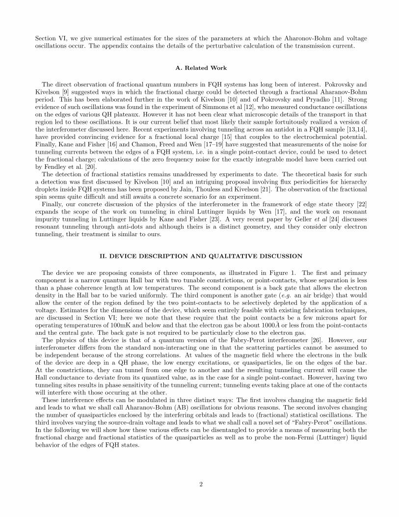
The device we are proposing consists of three components, as illustrated in Figure 1. The first and primarycomponent is a narrow quantum Hall bar with two tunable constrictions, or point-contacts, whose separation is lessthan a phase coherence length at low temperatures. The second component is a back gate that allows the electrondensity in the Hall bar to be varied uniformly. The third component is another gate (e.g. an air bridge) that wouldallow the center of the region defined by the two point-contacts to be selectively depleted by the application of avoltage. Estimates for the dimensions of the device, which seem entirely feasible with existing fabrication techniques,are discussed in Section VI; here we note that these require that the point contacts be a few microns apart foroperating temperatures of 100mK and below and that the electron gas be about 1000A or less from the point-contactsand the central gate. The back gate is not required to be particularly close to the electron gas.

The physics of this device is that of a quantum version of the Fabry-Perot interferometer [26]. However, ourinterferometer differs from the standard non-interacting one in that the scattering particles cannot be assumed tobe independent because of the strong correlations. At values of the magnetic field where the electrons in the bulkof the device are deep in a QH phase, the low energy excitations, or quasiparticles, lie on the edges of the bar.At the constrictions, they can tunnel from one edge to another and the resulting tunneling current will cause theHall conductance to deviate from its quantized value, as in the case for a single point-contact. However, having twotunneling sites results in phase sensitivity of the tunneling current; tunneling events taking place at one of the contactswill interfere with those occuring at the other.

These interference effects can be modulated in three distinct ways: The first involves changing the magnetic fieldand leads to what we shall call Aharanov-Bohm (AB) oscillations for obvious reasons. The second involves changingthe number of quasiparticles enclosed by the interfering orbitals and leads to (fractional) statistical oscillations. Thethird involves varying the source-drain voltage and leads to what we shall call a novel set of “Fabry-Perot” oscillations.In the following we will show how these various effects can be disentangled to provide a means of measuring both thefractional charge and fractional statistics of the quasiparticles as well as to probe the non-Fermi (Luttinger) liquidbehavior of the edges of FQH states.

2

V G

VGV G

t 1I t 2

VC

I

GV

R

L

R

L

ΦR

L

FIG. 1. Two point-contact interferometer. Two gates are placed a distance a apart. The gate voltages are adjusted so as tobring the edges of a FQH state with filling fraction ν close together, but not pinch the constriction. In this way, quasiparticlescarrying fractional charge and statistics can tunnel from one edge to the other. A magnetic flux Φ can be inserted in the regionbetween the point-contacts that is bounded by the edge states. A central gate allows the charge in the region to be selectivelydepleted. The transmitted current (the Hall current IH = νe2/h minus the tunneling current I1

t + I2t ) oscillates as a function

of the inserted flux, the voltage difference between the edges and the voltage of the central gate. An overall back gate on thedevice allows magnetic field sweeps at constant filling factor.

We would like to emphasize that we will always be interested in the limit where the barriers are weak, so that theconstrictions are far from being pinched off, as in Figure 1. (The opposite limit, where the two point-contacts arenear pinch off, is similar to tunneling through a quantum dot, except that for our geometry the central island wouldbe larger. It can be analyzed using methods similar to those in this paper, but we will not address it here.) Thechief advantage of this restriction is that we stay far from the regime near pinch off where, experimentally, poorlyunderstood resonances arise already for a single point-contact [27]. Consequently, we expect that the only resonancesare the ones explicitly created by the two point-contact geometry and the resulting energy and field scales for these areset by the parameters of the device and can be chosen to lie in an observable range. (Given the lack of understandingof the near pinch-off resonances, it is hard to say theoretically whether they are absent for weak barriers; however,experiments involving antidot resonances [13,14] do strongly suggest this.) Further, it becomes possible to probe theinternal structure of the resonance, i.e. its intermediate energy behavior, without detailed microscopic knowledge.Another restriction on our analysis is that we consider only the primary Hall states, i.e. ν = 1/m with m odd, wherethere is only one branch of edge excitations and life is somewhat simpler; the extension to their descendant statesdoes not pose any conceptual problems.

A. Aharonov-Bohm and fractional statistics oscillations

We will first discuss the interference effects which occur when the magnetic field is varied. Consider the transmissionamplitude for quasiparticles propagating along the right edge. As they can tunnel to the left edge at the twoconstrictions in Fig. 1, the amplitude will involve a sum over paths that encircle the area A enclosed by the edgesand the constrictions any number of times. As a result, they pick up an AB phase proportional to the flux Φ throughthis area. Naively, this phase is given by 2πe∗BA/(hc), where e∗ is the charge of the quasiparticle. It is convenient todefine an effective flux quantum by Φ∗ = e

e∗Φ0, where the usual flux quantum is given by Φ0 = hc/e. Then, in terms

of this effective flux quantum, we would expect that as the magnetic flux is varied, the current and other properties ofthe system would undergo oscillations with period ∆B∗ = Φ∗/A, and thus measurements of these oscillations wouldprovide a means of measuring the fractional charge.

However, this conclusion is too naive. The quasiparticles derive their properties from the parent liquid which isthe relevant “vacuum” and only when the vacuum is invariant can we expect to use arguments based solely on theirAB phases. Indeed, if the extra flux added is dynamically localized in the interior of the fluid this would effectivelycreate a multiply connected geometry where gauge invariance for the constituent electrons implies a flux periodicityof ∆B = Φ0/A. As this is smaller than the quasiparticle period ∆B∗, this would exclude oscillations with the latterperiodicity. We should emphasize that this is a dynamical possibility, there are no general, non-trivial consequences ofgauge invariance for the geometry at issue here. At any rate, it is clear that we need to be careful about consideringchanges in the bulk of the fluid as the flux is varied. To this end we distinguish between two cases.i)Field sweeps at fixed particle number: In this case, as we just observed, we expect to observe conductance oscillations

3

with period Φ0/A. This can happen in one of two ways depending upon the detailed electrostatics of the central region.If, as the magnetic field is raised, the QH fluid in the central region shrinks uniformly in order to keep the filling fractionconstant, then its area decreases by just the right amount to leave the flux through the whole droplet unchanged.Consequently, there are no oscillations as the magnetic field is varied and the period is trivially Φ0/A. If, instead,the electrostatics prefers otherwise and the self-consistent potential has a maximum in the interior, quasiholes willbe created there as the magnetic field is increased—one quasihole for each flux quantum. The phase picked up by aquasiparticle encircling the central region is now the sum of the fractional AB phase and the phase −θ∗ = −2π/mdue to its (fractional) statistical interaction with the central quasihole and precisely restores the periodicity to ∆B.ii)Field sweeps at fixed filling factor: One obtains quite different results if the field is swept at fixed filling factor. Inthis case the quasiparticles see an invariant vacuum (in other words, the electron density is changed so that quasiholesare not formed in the bulk of the droplet). The resulting periodicity is then ∆B∗. The observation of conductanceoscillations with such a fractional AB period would constitute a measurement of a fractional AB charge for thequasiparticles. Experimentally, keeping the filling factor constant requires changing the number of particles alongwith the field which is why the device requires a back gate. Also, preventing the formation of quasiholes in the centralregion requires that net fractional charge be added to the this area, which is only possible if the contacts are notpinched off.

Having discussed the observation of fractional charge we now turn to the observation of fractional statistics. Wefirst note that the comparison between the periodicity ∆B when the number density n of electrons is held constantand the periodicity ∆B∗ when the filling fraction ν is held constant, implicitly verifies the fractional statistics of thequasiparticles and quasiholes, because in one case the period is due to the combined effects of the Aharonov-Bohmphase and fractional statistics, and in the second it is due only to the Aharonov-Bohm phase.

To more directly see the effect of the fractional statistics, we need to consider oscillations that arise from havingvarying numbers of quasiparticles in the central region. If N quasiholes are present, then the interference phase ismodified to 2π(BA/Φ∗ −N/m). It is clear then that it is neccessary to add m quasiparticles before the interferencecondition is restored. To this end one can imagine using the central gate to deplete the central region in steps ofcharge 1/m which would then lead to conductance oscillations with a period of m steps. A better strategy, whichrequires less control over the electrostatics, is to create some unknown number of quasiholes in the central region andthen look for a shifted fractional AB pattern at fixed filling factor, as in the charge measurement. Except when aninteger multiple of m quasiholes are present, there will be a shift in this pattern and the observation of m− 1 distinctshifts will be a direct signature of the statistical interaction between the quasiparticles. For example, at ν = 1/3,there will be two shifted patterns with shifts of (1/3)∆B∗ and (2/3)∆B∗.

B. Fabry-Perot oscillations due to finite source-drain voltages

The third modulation of the interference appears when varying the source-drain voltage V , and again leads tooscillations in the conductance. The origin of these oscillations is most transparent for ν = 1, where single-particleconsiderations suffice; this is detailed in Section IV. In brief, the conductance at finite V is determined by the trans-mission of electrons in a range of energies ∆E = eV while the transmission itself oscillates with energy. Consequently,the integrated transmission, and hence the conductance itself, oscillates with the source-drain voltage, albeit with anenvelope that decreases as 1/V .

An interesting perspective is afforded by thinking in analogy to the classical wave analysis of the Fabry-Perotinterferometer, i.e. a device with two parallel partially transmitting barriers; as we shall see in the edge state analysisof the device, it is conceptually exact and allows a unified treatment of the fractional fillings as well. Evidently,the combination ωosc = 2π/τ , the inverse time for edge waves (and hence the quasiparticles) to travel from onepoint-contact to the other, is the characteristic frequency of the device and will set the scale for the oscillations inits transmission due to multiple reflections within it. The source-drain voltage defines a second frequency scale, theJosephson frequency ωJ = e∗V/h, where e∗ is the fractional charge of the quasiparticles living on the edges; this isthe bandwidth of the waves incident on the interferometer. It follows then that the transmission will be a function ofthe ratio ωJ/ωosc as well as of the reflection/transmission coefficients at the point-contacts which are determined bythe quasiparticle tunneling amplitudes at them.

Because the right-moving and left-moving waves lie on the edge of a QH droplet, there is a second perspective thatis very illuminating. (This picture, however, is not as general as the actual calculation of the voltage oscillations, sincethe calculation does not explicitly require the left- and right-moving edges to enclose any amount of flux; it would alsobe valid for a 1D wire if the modes were to have differing chemical potentials.) In this picture, the Aharonov-Bohmphase is responsible for the oscillations in the transmission as the energy is varied because the different energies leadto different areas enclosed by the interfering orbits. More specifically, an increase in energy of δE corresponds to a

4

change in the momentum of the quasiparticles given by δk = νδE/(hv), where v is the velocity of the edge modes[28]. The momentum at the edge is related to the area of the droplet A and its perimeter 2a by k = νA/(l22a), wherel is the magnetic length, so that an increase of δE in energy results in an increase in area of δA = 2l2aδE/(hνv). Theextra flux enclosed then gives a change in phase of 2πδΦ/Φ∗

0 = 2aδE/hv = 4πδE/hωosc. As a result, as the energy isvaried, the transmission oscillates with a period set by ωosc [29].

Three conclusions follow from this description. First, we recover the result that the net transmission has a compo-nent that oscillates with the source-drain voltage. Second, we find that there are two distinct regimes as a functionof ωJ/ωosc. For small values of this ratio the device is probed at low frequencies and hence at a long length scalewhere the coherence between the two barriers is important. In this regime the phase difference between the reflec-tion/transmission coeffecients at the barriers governs the transmission. Because this phase difference is determinedby the AB phase, the AB oscillations discussed in the previous section will occur. At large values of the ratio, thebarriers enter independently and the AB oscillations are washed out. The third and most interesting conclusion isthat even for intermediate values of the ratio there are special points where the AB oscillations disappear. Again, theorigin of this disappearance is most transparent for ν = 1: the nodes occur whenever the bandwidth is equivalent to aphase difference of an integer multiple of 2π across it. In such cases the phase shift between the barriers is immaterial;essentially, one is integrating the interference pattern over an integral number of periods, so the oscillations cancel.

The detailed analysis in Section III, where we consider the case of general ν, bears out the same qualitative featurethat there are special values of V where the AB oscillations disappear. However, the location of these nodes ismodified in a very interesting way which depends sensitively upon the nature of correlations in the edges. If the edgedynamics are of the Fermi liquid variety, as should be the case at ν = 1, our naive assertions are correct. However,if the edges are Luttinger liquids then the locations of the nodes are given by the zeros of Bessel functions whichdepend on ωJ/ωosc, and the type of Bessel function depends on the Luttinger liquid exponent g. The nodes occurfor ωJ/ωosc ≈ (n+ ξg)/2, n = 0, 1, . . ., with the g dependent shift ξg = (1 + g)/2. For quasiparticle tunneling, whereg = ν, this shift is not an integer, and can, in principle, be used to measure g! (Given an independent measurementof v, this also allows a measurement of e∗.) Thus it follows that the interferometer can also be used to distinguishbetween Fermi liquid (with g = 1) and Luttinger liquid behavior at the edges of FQH systems.

In the qualitative discussions of the Aharonov-Bohm and Fabry-Perot oscillations above, we have considered thezero temperature case for simplicity. The effects of finite temperature, particularly the suppression of quantuminterference, are treated quantitatively in Section V.

III. TUNNELING BETWEEN EDGE STATES IN THE DOUBLE POINT-CONTACT GEOMETRY

We will now study the interferometer in the framework of edge states in the quantum Hall effect, which is bettercast in the bosonic language (for a thorough review, see Ref. [22]). Our starting point for studying tunneling in adouble point-contact geometry is the Lagrangian density

L =1

8π[(∂tφ)2 − v2(∂xφ)2] −

∑

i=1,2

Γi e−iωJ t δ(x− xi) e

i√

gφ(t,xi) +H.c. , (1)

with the quantization condition [φ(t, x), ∂tφ(t, y)] = 4πiδ(x − y). (We use this normalization of φ because it givesan especially simple expression for the dimensions of the tunneling operators in terms of g. To translate to theconventional normalization of a 1D electron gas or the sine-Gordon model, φ must be replaced by φ/(2

√π).) The

voltage difference between the two edges of the QH liquid determines the Josephson frequency ωJ ≡ e∗V/h, withe∗ = e for electron tunneling and e∗ = e/m for quasiparticle tunneling. In the following we will set the edge velocityv = 1. The two point-contacts are located at x1 and x2, and their tunneling amplitudes are Γ1 and Γ2, respectively[30].

The first term in the Lagrangian, when considered alone, describes the dynamics of a free boson field φ = φR +φL,which can be decomposed into its chiral components φR,L. These components describe right and left moving excitationsalong the edges of FQH states. Charge density operators can be defined in terms of the φR,L through ρR,L =

e√

ν2π ∂xφR,L.The second term in the Lagrangian comes from the tunneling between the edges. The tunneling operators can be

written as Ψ†LΨR and Ψ†

RΨL. Right and left moving electron and quasiparticle operators on the edges of a FQH liquid

are given by ΨR,L(t, x) ∝ e±i√

gφR,L(t,x) e±ikF x, where g is related to the FQH bulk state. For example, for a Laughlinstate with filling fraction ν = 1/m we have g = m for electrons and g = 1/m for quasiparticles carrying fractional

charge e/m. One can verify that [ρR,L(t, x) , Ψ†R,L(t, y)] = e

√νg Ψ†

R,L(t, y)δ(x− y), so that indeed the cases g = ν−1

and g = ν correspond to the electron (e∗ = e) and quasiparticle (e∗ = νe) creation operators, respectively.

5

The flux Φ in the area enclosed by the edge branches between the two point-contacts is taken into account bythe phase of the tunneling amplitudes, Γi, in Equation (1) . This phase comes from the quasiparticle’s momentum

kf in the definition of ψR,L. From this definition, the tunneling operator ψ†L(x)ψR(x) has the phase e2ikf x, where

2kf is equal to the momentum difference between the right-moving edge and the left-moving edge. The momentumdifference 2kfe between electrons on the two edges is directly related to the perimeter L and area A of the QHliquid confined between the two point-contacts. It is given by kfeL = 2πBA/Φ0. If the distance between the twoedges at each of the point-contacts is much smaller than the distance a along an edge between the two contacts,then the perimeter can be set equal to 2a. For ν = 1/m, with m an integer, the momentum of the quasiparticlesis then given by 2kf = ν2kfe = 2πΦ/(Φ∗a). Because Γ1 is the amplitude for tunneling at x = −a/2, it has the

phase ei2πΦ/(2Φ∗), and similarly Γ2 has the phase e−i2πΦ/(2Φ∗). Thus, the flux can be introduced in Equation (1) bytaking Γ1,2 = Γ1,2e

±i2πΦ/(2Φ∗), where Γ1,2 are couplings which do not include the phase due to the magnetic flux.Combining these together, we find that a quasiparticle that circles the area between the two constrictions once (bytunneling from the left-moving edge to the right-moving edge at x = −a/2 and tunneling back to the left-moving edgeat x = a/2) picks up the amplitude Γ∗

1Γ2 = Γ∗1Γ2e

−2πiΦ/Φ∗

, so that the phase of the tunneling amplitudes determinesthe Aharonov-Bohm phase.

The form of the phases appearing in the amplitudes Γ1 and Γ2 can also be viewed as coming from the interactionof the bosonic edge states φ with the electric and magnetic fields. In particular, the electric and magnetic potentialsact as sources which the field φ interacts with via its optical charge

√νe [25]. In this way, one can show that the full

phase due to the magnetic flux Φ and the N quasiholes in the area between the two constrictions can be accounted forby taking Γ∗

1Γ2 = Γ∗1Γ2e

−i2π(Φ/Φ∗−Nν), when ν is equal to one over an integer. Then, according to Section II, the fullphase will depend on exactly how the magnetic field is varied; if the electron number density is held fixed, the phaseis the “electron” Aharonov-Bohm phase Φ/Φ0, and if the filling fraction is held fixed, the phase is the “quasiparticle”Aharonov-Bohm phase Φ/Φ∗.

In the absence of tunneling, the current I equals the Hall current IH = νe2/hV . In the presence of tunneling,the transmission current I satisifies I = IH − It, where It is the tunneling current. Treating the tunneling termperturbatively in the model above, we can solve for the tunneling current It as a function of the voltage V betweenthe edges, to low orders in the tunneling amplitude. This perturbative result is valid as long as It is small comparedto the Hall current IH . It is easy to generalize the problem to N contacts located at xi with tunneling amplitudes Γi,for i = 1, .., N , and in appendix A we solve this general problem. The result can be cast in a form very similar to theone point-contact result. At zero temperature, it is given by

It = e∗|Γeff |22π

Γ(2g)|ωJ |2g−1 sign(ωJ) , (2)

where, for several point-contacts, Γeff is the effective coupling which includes the interference between the couplingsΓi, i = 1, .., N . The effective coupling is given by

|Γeff |2 =

N∑

i,j=1

Γi Γ∗j Hg(ωJ |xi − xj |) , (3)

with

Hg(x) =√π

Γ(2g)

Γ(g)

Jg−1/2(x)

(2x)g−1/2, (4)

where Jg−1/2 is a Bessel function of the first kind. In the case of a single point-contact, the effective coupling is givenby Γeff = Γ, independent of frequency, and we recover the familiar results of Ref. [17].

In the case of the two point-contact geometry, we have an effective coupling

|Γeff |2 = |Γ1|2 + |Γ2|2 + (Γ1Γ∗2 + Γ∗

1Γ2) Hg(ωJa

v) , (5)

where a = |x1 − x2| is the linear distance along the edge between the contacts, and we have restored the velocityv to the equation. (If the path length between the point-contacts for the left and right edges are different, then ais the average of the two lengths and there is an extra contribution to the relative phase between Γ1 and Γ2.) Theseparation a sets the time scale τ = a/v, and thus the frequency scale ωosc = 2π/τ for oscillations in the value of theeffective coupling Γeff . It is easy to check that Hg(x) → 1 as x → 0, and that Hg(x) → 0 as x → ∞, so that theeffective coupling has the asymptotic values

6

|Γeff |2 =

|Γ1 + Γ2|2 , ωJ ≪ ωosc

|Γ1|2 + |Γ2|2, ωJ ≫ ωosc

which correspond to coherent and incoherent interference between Γ1 and Γ2. In the first case Γeff depends on therelative phase between Γ1 and Γ2, so the tunneling current should clearly exhibit the Aharonov-Bohm oscillations,and in the second case the Aharonov-Bohm effect is washed out.

For the intermediate range of frequencies comparable to ωosc, there will be oscillations in the effective coupling asa function of ωJ . This interference term depends on the relative phase between Γ1 and Γ2, which can be adjusted byvarying the magnetic flux Φ through the area between the two point-contacts. If an experimental aparatus is setupto detect the component of the current that oscillates with the flux Φ, the magnitude of the oscillations will be

|IΦt | = e∗|Γ1||Γ2|

2π

Γ(2g)|ωJ |2g−1 |Hg(

ωJa

v)| . (6)

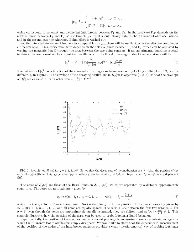
The behavior of |IΦt | as a function of the source-drain voltage can be understood by looking at the plot of Hg(x), for

different g, in Figure 2. The envelope of the decaying oscillations in Hg(x) is algebraic (∼ x−g), so that the envelope

of |IΦt | scales as ωg−1

J , or in other words, |IΦt | ∝ V g−1.

0 1 2 3 4 5 6-1.0

-0.8

-0.6

-0.4

-0.2

0.0

0.2

0.4

0.6

0.8

1.0

g=1 g=1/3 g=1/5

Hg(

x)

x/2π

FIG. 2. Modulation Hg(x) for g = 1, 1/3, 1/5. Notice that the decay rate of the modulation is x−g. Also, the position of thezeros of Hg(x) (those of Jg−1/2(x)) are approximately given by xn ≈ π(n + ξg), n integer, where ξg = 1+g

2is a g dependent

shift

The zeros of Hg(x) are those of the Bessel function Jg−1/2(x), which are separated by a distance approximatelyequal to π. The zeros are approximately given by

xn ≈ π(n+ ξg) , n = 0, 1, . . . with ξg =1 + g

2, (7)

which fits the graphs in Figure 2 very well. Notice that for g = 1, the position of the zeros is exactly given byxn = π(n + 1), n = 0, 1, . . ., and all zeros are equally spaced. The ratio x1/x0 between the first two zeros is 2. Forg 6= 1, even though the zeros are approximately equally separated, they are shifted, and x1/x0 ≈ g+3

g+1 6= 2. This

example illustrates how the position of the zeros can be used to probe Luttinger liquid behavior.Experimentally, the position of these nodes can be observed precisely by measuring those source-drain voltages for

which the Aharonov-Bohm oscillations simply disappear. We would like to stress that the experimental measurementof the position of the nodes of the interference patterns provides a clean (interferometric) way of probing Luttinger

7

liquid behavior. Such an interferometric measurement focuses on the behavior between the two contacts, and may befree of parasitic effects elsewhere that can mask the anomalous scaling behavior of Luttinger liquids.

Finally, the location of the nodes could also provide another method of measuring fractional charge. The positionof the nodes depends on ωJa/v, where the Josephson frequency ωJ = e∗V/h depends on the fractional charge. Ifthere were an independent measurement of the velocity the of edge modes v, then the location of the nodes wouldyield a value for e∗.

IV. FREE FERMIONS

To better understand the behavior of our perturbative solution for the current, we will look at the exact solutionfor the g = 1 case with two constrictions. This case reduces to a simple problem that is essentially the same as wavetransmission through a Fabry-Perot interferometer. We can solve for the transmission and reflection amplitudes ata single impurity, which, for g = 1, are independent of the energy of the incident waves. Then, in addition to usingthese amplitudes to account for the scattering at each of the two impurities, we must also propagate the waves fromone impurity to another, which is the part responsible for the interference effects. Each frequency ω will then betransmitted with a different coefficient T (ω). For an applied voltage V between the edges, there will be a wholerange of frequencies of width ωJ = eV/h in the incident wave packet. We must then integrate the final transmissioncoefficients over the energies in this band that contribute to the total current.

Consider, to begin with, a single point-contact with tunneling amplitude Γ, which can either transmit or scatter aparticle. For g = 1, we can work in terms of free fermions given by ψR,L = 1√

2πe±iφR,L(x,t), with Hamiltonian

H =

∫

d x

{

ψR†(x)

[

−i ∂∂x

− ω0

2

]

ψR(x) + ψL†(x)

[

i∂

∂x+ω0

2

]

ψL(x)

+ 2πδ(x)[

ΓiψL†(x)ψR(x) +H.c.

]

}

. (8)

Once again, we have set the velocity v of the chiral fermions to 1. It is then a straightforward wave mechanics problemto solve for the scattering matrix, S, which gives the transformation from the incoming modes, ψR−(ω), ψL+(ω) to the

outgoing modes, ψR+(ω), ψL−(ω). We find that S =

(

ti ri−ri∗ ti

)

, where the transmission and reflection amplitudes

are given by

ti =1 − π2|Γi|21 + π2|Γi|2

and ri =−i2πΓi

∗

1 + π2|Γi|2. (9)

The transmission and reflection coefficients are T = |t|2 and R = |r|2, respectively. (We note here that Γi in Equation9 is renormalized so that the strong barrier limit or total reflection (R = 1) occurs when |Γi| = 1/π. This is in contrastwith the case when g = 1/2 or 1/3, when total reflection occurs as Γ → ∞. Technically, this difference arises becausefor g < 1 the tunneling operator is infrared relevant whence short distance behavior does not matter, whereas forg = 1 it is marginal.)

When there is more than one scatterer, it is convenient to use the transmission matrix approach to find the trans-mission through and reflection out of the two point-contacts separated by a distance a. Recall that the transmissionmatrixMi gives the transformation from the states on the left of the barrier, ψR−(ω), ψL−(ω), to the states on the right

of the barrier, ψR+(ω), ψL+(ω), and can be obtained directly from S. After passing through the first constriction, the

waves propagate to the right a distance a, which results in multiplying the modes

(

ψR(ω)

ψL(ω)

)

by D =

(

eiaω 00 e−iaω

)

.

Finally, the waves are scattered again by the second point-contact, so the waves on the right-hand side depend on thewaves to the left of the scatterers as follows:

(

ψR+(ω)

ψL+(ω)

)

= M2DM1

(

ψR−(ω)

ψL−(ω)

)

. (10)

Note that the matrix D contains the phase e±iωx, and it is this phase which is responsible for the voltage oscillations.In particular, the right-moving and left-moving modes that scatter between the two point-contacts have oppositephases which interfere with each other. Multiplying out the matrices in Eq. (10), we find that the transmissionamplitude for the two point-contact geometry is

8

t(ω) =t1t2

1 + r1r∗2e2iωa

, (11)

where t1,2 and r1,2 are the transmission and reflection amplitudes for the two contacts, as given by Eq. (9). Thetransmission coefficient T (ω) through the whole droplet is then

T (ω) =|t1|2|t2|2

1 + |r1|2|r2|2 + (r1r∗2e2iωa + r∗1r2e

−2iωa). (12)

With this frequency dependent transmission coefficient, we can calculate the current for an energy difference ωJ

between the right and left moving edges. It is given by the total right-moving current minus the total left-movingcurrent passing through a point x. If we choose the point to be to the right of the barrier, then the total right-movingcurrent at energy ω is given by the transmitted right-moving current eT (ω)nR(ω) plus the total left-moving currentthat was reflected into right movers e[1−T (ω)]nL(ω). Similarly, the total left-moving current at energy ω is just thetotal incoming left-moving current nL(ω), where nR,L(ω) are the occupation numbers of right and left movers. Inthis simple model we can easily include the temperature dependence of the transmission because it can be completelyaccounted for by the Fermi-Dirac distribution of the left and right movers:

nR,L(ω) =1

eβ(ω∓ωJ/2) + 1. (13)

The expression for the current through the droplet then reduces to

I = e

∫ ∞

−∞

dω

2πT (ω)

[

nR(ω) − nL(ω)]

. (14)

At zero temperature, the integral in Eq. (14) yields

I =e

2πa

|t1|2|t2|21 − |r1|2|r2|2

tan−1

1−|r1|2|r2|21+|r1|2|r2|2 sin(ωJa)

cos(ωJa) +r1r∗

2+r∗

1r2

1+|r1|2|r2|2

. (15)

Notice that if t1 = t2 = 1 (total transmission), I = e2πωJ = e2

h V . For small tunneling amplitutes Γ1 and Γ2

(|r1|2, |r2|2 ≪ 1), we find that I = e2

h V − It, where

It = e∗|Γeff |2 2πωJ , (16)

with

|Γeff |2 = |Γ1|2 + |Γ2|2 + (Γ1Γ∗2 + Γ∗

1Γ2)sin(ωJa)

(ωJa). (17)

This is the same as the result obtained perturbatively in section III if we set g = 1 in Eq. (5).If we expand the transmission coefficient T (ω) in Eq. (12) for small tunneling amplitudes, we can easily obtain the

finite temperature tunneling current It. It is still given by Eq. (16), but the effective coupling is now

|Γeff |2 = |Γ1|2 + |Γ2|2 + (Γ1Γ∗2 + Γ∗

1Γ2)2πTa

sinh(2πTa)

sin(ωJa)

(ωJa). (18)

Notice that the distance a sets the temperature scale for which the interference term Γ1Γ∗2 + Γ∗

1Γ2 decays.In the general case, such as for other filling fractions, the current should still be obtainable by an expression like

Equation 14, where T (ω) is the transmission coefficient and nR(ω) and nL(ω) are the number densities of filled statesat energy ω. If the behavior of the system deviates from the result in Equation 15, this should indicate that thetransmission and reflection amplitudes for a single point-contact depend on energy and that the density of states nolonger has the simple Fermi-liquid form.

9

V. FINITE TEMPERATURE EFFECTS

In section III we have found that, at zero temperature, the effect of the two point-contacts can be completelyabsorbed into an effective coupling Γeff , which describes all the interference between the two contacts. In this sectionwe will show that when T 6= 0, this is still the case, but now Γeff will depend on temperature also.

The finite temperature T brings another energy scale to the problem. This energy scale should be compared tothe one set by the separation between the contacts a, which is given by ωosc = 2πv/a. Thus, when kT ≫ hωosc,the interference effects should be washed out. One should also keep in mind the energy scale associated with theJosephson frequency ωJ = e∗V/h, so that the decay of the interference effects with temperature will depend on theratios of the three energy scales T , ωJ and ωosc. The interesting question to ask is how the different g affect the waythe interference is washed out, or, equivalently, how the filling factor ν of the underlying FQH state affects the decayof the oscillations with temperature.

To lowest order in the tunneling amplitude Γ, the tunneling current between edge states in the presence of a singlepoint-contact at finite temperature is given by [17]:

It = e∗ |Γ|24(πT )2g−1 B(

g − iωJ

2πT, g + i

ωJ

2πT

)

sinh(ωJ

2T

)

, (19)

where B is the beta function. In appendix A we show that the same expression gives the current for N point-contactswith couplings Γi, i = 1, ..., N if we use an effective coupling

|Γeff |2 =

N∑

i,j=1

Γi Γ∗j Hg(ωJ , |xi − xj |, T ) , (20)

with

Hg(ωJ , x, T ) = 2πΓ(2g)

Γ(g)

e−2gπT |x|

sinh ωJ

2T

× Im

{

e−iωJ |x| F (g, g + i ωJ

2πT ; 1 + i ωJ

2πT ; e−4πT |x|)

Γ(g − i ωJ

2πT ) Γ(1 + i ωJ

2πT )

}

. (21)

In this expression, F is a hypergeometric function. Notice that the function Hg depends on T , x and ωJ only throughthe combinations ωJx and ωJ/(2πT ). We can thus cast the modulation Hg

(

ωJx,ωJ

2πT

)

in terms of the followingfunction of two variables:

Hg(y1, y2) = 2πΓ(2g)

Γ(g)

e−gy1/y2

sinh(πy2)× Im

{

e−iy1 F (g, g + iy2; 1 + iy2; e−2y1/y2)

Γ(g − iy2) Γ(1 + iy2)

}

. (22)

The effective coupling for a two point-contact geometry is then

|Γeff |2 = |Γ1|2 + |Γ2|2 + (Γ1Γ∗2 + Γ∗

1Γ2) Hg

(

2πωJ

ωosc,ωJ

2πT

)

. (23)

In this form, it is clear that the interference term depends on the ratios of the three energy scales in the problem.We begin to explore how different values of g change the behavior of the modulation Hg by considering Fermi liquid

(g = 1) edge states associated with a QH filling factor ν = 1. In this case, Eq. (22) can be shown to simplify to

H1(y1, y2) =y1/y2

sinh(y1/y2)

sin y1y1

, (24)

so that

|Γeff |2 = |Γ1|2 + |Γ2|2 + (Γ1Γ∗2 + Γ∗

1Γ2)4π2T/ωosc

sinh(4π2T/ωosc)

sin(2πωJ/ωosc)

(2πωJ/ωosc). (25)

This is the same as the expression obtained in section IV directly from the free fermion transmission approach. Noticethat for g = 1 the finite temperature correction appears only as a multiplicative factor in front of the modulationfor T = 0. This is not necessarily the case for other g, as shown below in Fig. 4. This multiplicative factor decaysexponentially (1/ sinh(4π2T/ωosc)) with temperature, with the scale (ωosc) set by the two point-contact separation a.In Fig. 3 we show the decay of Hg with temperature for ωJ = 0 in a log-plot. From this plot we can extract how themodulation decays with temperature T for different g. Using asymptotic expressions for the hypergeometric function,

10

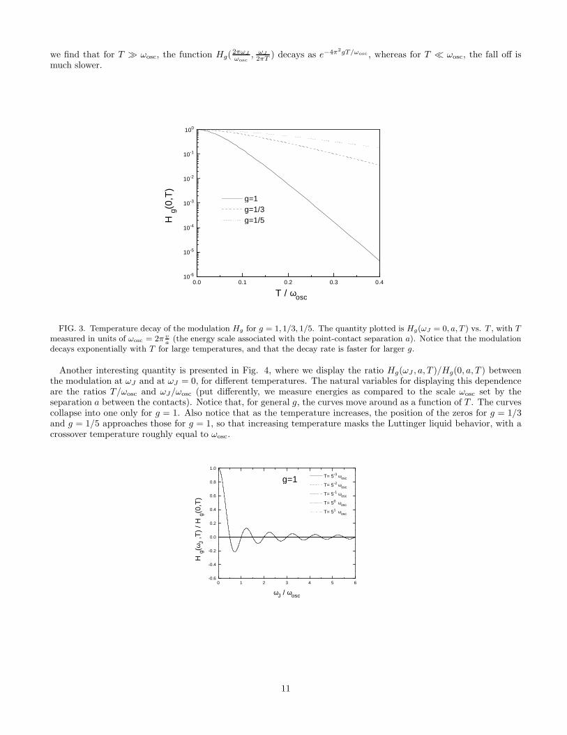
we find that for T ≫ ωosc, the function Hg(2πωJ

ωosc

, ωJ

2πT ) decays as e−4π2gT/ωosc , whereas for T ≪ ωosc, the fall off ismuch slower.

0.0 0.1 0.2 0.3 0.410-6

10-5

10-4

10-3

10-2

10-1

100

g=1 g=1/3 g=1/5H

g(0,

T)

T / ωosc

FIG. 3. Temperature decay of the modulation Hg for g = 1, 1/3, 1/5. The quantity plotted is Hg(ωJ = 0, a, T ) vs. T , with Tmeasured in units of ωosc = 2π v

a(the energy scale associated with the point-contact separation a). Notice that the modulation

decays exponentially with T for large temperatures, and that the decay rate is faster for larger g.

Another interesting quantity is presented in Fig. 4, where we display the ratio Hg(ωJ , a, T )/Hg(0, a, T ) betweenthe modulation at ωJ and at ωJ = 0, for different temperatures. The natural variables for displaying this dependenceare the ratios T/ωosc and ωJ/ωosc (put differently, we measure energies as compared to the scale ωosc set by theseparation a between the contacts). Notice that, for general g, the curves move around as a function of T . The curvescollapse into one only for g = 1. Also notice that as the temperature increases, the position of the zeros for g = 1/3and g = 1/5 approaches those for g = 1, so that increasing temperature masks the Luttinger liquid behavior, with acrossover temperature roughly equal to ωosc.

0 1 2 3 4 5 6-0.6

-0.4

-0.2

0.0

0.2

0.4

0.6

0.8

1.0

g=1 T= 5-3 ωosc

T= 5-2 ωosc

T= 5-1 ωosc

T= 50 ωosc

T= 51 ωosc

H g(

ωJ

,T)

/ H

g(0,

T)

ωJ / ωosc

11

0 1 2 3 4 5 6-0.6

-0.4

-0.2

0.0

0.2

0.4

0.6

0.8

1.0

g=1/3 T= 5-3 ωosc

T= 5-2 ωosc

T= 5-1 ωosc

T= 50 ωosc

T= 51 ωosc

H g(

ωJ

,T)

/ H

g(0,

T)

ωJ / ωosc

0 1 2 3 4 5 6-0.6

-0.4

-0.2

0.0

0.2

0.4

0.6

0.8

1.0

g=1/5 T= 5-3 ωosc

T= 5-2 ωosc

T= 5-1 ωosc

T= 50 ωosc

T= 51 ωosc

H g(

ωJ

,T)

/ H

g(0,

T)

ωJ / ωosc

FIG. 4. Dependence of the modulation Hg(ωJ , a, T ) on ωJ for different T . The quantity plotted is the rescaled Hg

(Hg(ωJ , a, T )/Hg(0, a, T )) so as to show how the shape of the modulation curve changes with T for different g. Notice that allcurves collapse for g = 1, i.e., all frequencies get suppressed uniformly as temperature is increased. For g = 1/3 and g = 1/5,however, notice that the curves do not collapse together anymore, and that higher ωJ are supressed more strongly than lowerωJ as T is increased.

VI. NUMERICAL ESTIMATES

In this section, we will give estimates of the sizes of parameters at which the interference effects could be observed.First, we will consider the change in magnetic field, ∆B, required for one Aharonov-Bohm period, which is given by

∆B =e

e∗Φ0

A=

e

e∗41µm2 gauss

A. (26)

If the number of electrons is held constant, then in this equation Φ0 is equal to one flux quantum and e∗ is the chargeof an electron, e. If, instead, the filling fraction is held fixed, then Φ0 is e/e∗ times one flux quantum, where e∗ isthe charge of the quasiparticle. In this equation, A is the area of the FQH liquid between the two contacts, and isroughly given by A = ad, where d is the width of the sample and a is the distance between the two contacts. If weassume the width is d = 1µm, then the period is related to the distance between the contacts by

∆B =

{

41µm− gauss/a for fixed number of electrons n120µm− gauss/a for fixed filling fraction ν = 1/3.

(27)

For a = 1µm or 10µm, the “electron” Aharonov-Bohm period is ∆B = 41 gauss and 4.1 gauss, respectively, and the“quasiparticle” Aharonov-Bohm period is ∆B = 120 gauss and 12 gauss, respectively.

Next, we consider the voltage fluctuations. The separation between the zeros of the Bessel function Jg−1/2(x) isapproximately equal to π and the location of the nodes in the voltage fluctuations roughly occur when

ωJa

v≈ π(n+ ξg) , n = 0, 1, . . . with ξg =

1 + g

2, (28)

As noted earlier, depending on the value of g, the precise location of these nodes will be shifted a little, which mayprovide a way of distinguishing between Luttinger liquid behavior and other types of behavior. In this equation, wehave restored the velocity of the edge modes v, which earlier was set to 1. For g = 1/3, an estimate for v [32] isv ≈ 105m/s. Using ωJ = e∗V/h, we find that the voltage at the nodes and the distance between the point-contactsmust satisfy

V a = (n+ ξg)e

e∗× 200µV − µm, (29)

where V has units of microvolts and a has units of microns. For ν = 1/3, we take e∗/e = 1/3. Thus, for a = 1µm or10µm the voltage at the first node is roughly 400µV and 40µV, respectively. Lastly, we will estimate the coherence

12

length, or the amount by which the temperature reduces the signal. However, we note that phonons can also lead todephasing, althought we do not consider them here. For temperatures greater than kT > hωosc/(4π

2), the interference

effects fall off as Te−4π2gkT/(hωosc), where ωosc = 2πv/a. Thus, for

kT <hv

2πga(30)

the signal is not affected much by temperature. We can define the coherence length, ac by the spacing for which thesignal has decreased roughly by a factor of 1/e, so that ac = vh/(g2πkT ). Then, for v ≈ 105m/s and g = 1/3, atT = 100mK the coherence length is ac = 4µm, and for T = 30mK, the coherence length is ac = 12µm. Thus, thesignal for a separation of 1µm should not be noticeably affected at either temperature, and even for a separation of10µm the signal will be attenuated by a factor of 2 at 30mK and by a factor of 15 at 100mK.

It follows then that a separation of a few microns should be sufficient to allow observation of the inteference effectsat temperatures around and below 100mK. The requirement on the gates is that they be close enough that theirelectrostatic “shadows” do not overlap in the plane of the electron gas. For gate diameters of about 1000A, thiscondition could be met by placing them about 1000A from the electron gas.

VII. CONCLUSIONS

In this paper we have proposed a device, the two point-contact interferometer, consisting of a Hall bar with two weakbarriers, that can be used to study quantum interference effects in a strongly correlated system. The device allows forthe study of three types of interference effects: Aharanov-Bohm oscillations with magnetic field, statistical oscillationswith quasiparticle number and Fabry-Perot oscillations with source-drain voltage. These interference effects can beused to measure the fractional charge and statistics of quasiparticles in the quantum Hall effect. They also provide anew way of searching for non-Fermi liquid behavior in the dynamics of the edges. We would like to emphasize thatmuch of our account of the physics of the device is quite robust, in that it depends upon quite general “topological”properties of QH quasiparticles; our proposals for measuring charge and statistics fall in this category. Other features,such as the details of the Fabry-Perot nodes are more specific to the simplest version of edge state dynamics usedin the calculations and as such are subject to the caveat that they represent the behavior of the system only at thelowest energies.

ACKNOWLEDGEMENTS

We would like to thank several colleages who gave us important suggestions and constructive criticism on theexperimental implications of this work: David Abusch-Magder, Ray Ashoori, Marc Kastner, Beth Parks and NikolaiZhitenev at MIT; Hari Manoharan, Kathryn Moler, Dan Shahar, Mansour Shayegan and Lydia Sohn at Princeton;Hong-Wen Jiang at UCLA. SLS would like to thank Phillip Phillips for introducing him to resonances in interactingsystems and for suggesting that the two barrier problem might be a good thing to look at. This work is supported byNSF grants DMR-94-00334 (CCC), DMR-93-12606 (SAK) and DMR-94-11574 (XGW). XGW and SLS acknowledgesupport from the A. P. Sloan Foundation. D. F. is currently a Bunting Fellow sponsored by the Office of NavalResearch.

APPENDIX A: PERTURBATIVE CALCULATION

We derive here the correction to the Hall current due to tunneling at the point-contacts. We will assume the generalcase of N contacts at locations xi and coupling Γi, i = 1, ..., N .

The first step in the calculation is to obtain the tunneling current operator j(t). This operator includes the tunnelingcurrents flowing from one edge to the other through all N point-contacts in the problem. The tunneling operator canbe obtained from the time evolution of the total charge operators QR,L on the R,L edges:

j(t) = − 1

ih[QL, H ] =

1

ih[QR, H ] . (A1)

The charge operator commutes with the free part of the Hamiltonian, so that the only contribution comes from thetunneling term

13

Htun =

N∑

i=1

Γie−iωJ tei

√gφ(t,xi) +H.c. . (A2)

Using the commutation relations for the bosonic fields φR,L, we obtain

j(t) = ie∗N

∑

i=1

Γiei√

gφ(t,xi) +H.c. . (A3)

The expectation value for the current at time t is given by

〈j(t)〉 = 〈0|S†(t,−∞) j(t) S(t,−∞)|0〉 , (A4)

where S(t,−∞) is the time evolution operator. The next step is to calculate 〈j〉 perturbatively in the tunneling ampli-tudes Γi. Because there is a voltage difference between the R and L terminals, the system is out of thermodynamicalequilibrium, and we must to use field theoretical tools appropriate for such non-equilibrium problems [18]. However,non-equilibrium effects appear only to second and higher orders in perturbation theory. Because we will calculate thetunneling current only to first order in perturbation theory, we will not have to use non-equilibrium field theory inthis particular calculation.

To lowest order in the tunneling perturbation we have

〈j(t)〉 = −i∫ t

−∞dt′ 〈0|[j(t), Htun(t′)]|0〉 . (A5)

In the calculation of

〈0|j(t) Htun(t′)|0〉 = e∗

N∑

i=1

N∑

j=1

〈0|(iΓie−iωJ tei

√gφ(t,xi) − iΓ∗

i eiωJ te−i

√gφ(t,xi))

× (Γje−iωJ t′ei

√gφ(t′,xj) + Γ∗

jeiωJ t′e−i

√gφ(t′,xj))|0〉 (A6)

the non-vanishing terms are those that transfer zero total charge when applied to |0〉. We then have

〈0|j(t) Htun(t′)|0〉 =

= ie∗N

∑

i,j=1

(

ΓiΓ∗j e

−iωJ (t−t′)〈0|ei√

gφ(t,xi)e−i√

gφ(t′,xj)|0〉 − Γ∗i Γj e

iωJ (t−t′)〈0|e−i√

gφ(t,xi)ei√

gφ(t′,xj)|0〉)

= ie∗N

∑

i,j=1

(ΓiΓ∗j e

−iωJ (t−t′) − Γ∗i Γj e

iωJ (t−t′)) eg〈0|φ(t,xi)φ(t′,xj)|0〉 . (A7)

The φ field correlation is

〈0|φ(t, x)φ(0, 0)|0〉 = 〈0|φR(t, x)φR(0, 0)|0〉 + 〈0|φL(t, x)φL(0, 0)|0〉 (A8)

= − ln[δ + i(t− x)] − ln[δ + i(t+ x)] ,

where δ is an ultraviolet cut-off scale. Let us define

Pg(t, x) = eg〈0|φ(t,x)φ(0,0)|0〉 =[

δ + i(t+ x)]−g ×

[

δ + i(t− x)]−g

. (A9)

Notice that Pg(t, x) = Pg(t,−x). Using the expression above, we can write

− i〈[j(t), Htun(t′)]〉 = e∗N

∑

i,j=1

(

ΓiΓ∗j e

−iωJ (t−t′) − Γ∗i Γj e

iωJ (t−t′))

×(

Pg(t− t′, xi − xj) − Pg(−t+ t′, xi − xj))

. (A10)

Inserting the above expression into Eq.(A5) and performing the t′ integration, we obtain the current expectationvalue:

14

〈j(t)〉 = e∗N

∑

i,j=1

ΓiΓ∗j + Γ∗

i Γj

2[Pg(ωJ , xi − xj) − Pg(−ωJ , xi − xj)] , (A11)

where Pg(ωJ , x) is the Fourier transform of the Pg(t, x) with respect to time. The problem is then reduced to the

calculation of the Pg’s. It is easy to calculate

Pg(ω, 0) =

∫ ∞

−∞dp

eiωp

(δ + ip)2g=

2π

Γ(2g)|ω|2g−1e−|ω|δ θ(ω) , (A12)

and we can express the case x 6= 0 in terms of the Pg(ω, 0):

Pg(ω, x) =

∫ ∞

−∞

dω′

2πPg/2(ω

′, 0) Pg/2(ω − ω′, 0) e−i(2ω′−ω)x (A13)

= θ(ω)

∫ |ω|

0

dω′

2πω′g−1 (ω − ω′)g−1 e−i(2ω′−ω)x

= Pg(ω, 0) Hg(ωx) ,

where

Hg(y) =√π

Γ(2g)

Γ(g)

Jg−1/2(y)

(2y)g−1/2. (A14)

The tunneling current between the edge states It = 〈j(t)〉 is then simply

It = e∗2π

Γ(2g)|ωJ |2g−1 sign(ωJ)

N∑

i,j=1

ΓiΓ∗j Hg(ω|xi − xj |) . (A15)

The expression for the tunneling current can be cast exactly in the same form as that for a single contact,

It = e∗|Γeff |22π

Γ(2g)|ωJ |2g−1 sign(ωJ) , (A16)

but with an effective coupling Γeff due to the interference between Γi, i = 1, .., N of the N contacts:

|Γeff |2 =

N∑

i,j=1

Γi Γ∗j Hg(ωJ |xi − xj |) . (A17)

The calculations for T = 0 can be extended for finite temperature. Basically, the algebraic correlations at T = 0are mapped to the correlations at T 6= 0 by a conformal transformation [31]:

1

[δ + i(t± x)]g→

[

πT

sin (πT [δ + i(t± x)])

]g

. (A18)

Using this transformation, we can recalculate the Pg’s and obtain their finite T version:

Pg(ω, x, T ) =

∫ ∞

−∞dt eiωt

[

sin (πT [δ + i(t+ x)])

πT

]−g [

sin (πT [δ + i(t− x)])

πT

]−g

(A19)

= (πT )2g

∫ ∞

−∞dt eiωt e−i π

2g[sign(t−x)+sign(t+x)]

[

sinh(πT |t− x|) sinh(πT |t+ x|)]−g

. (A20)

What we need for the calculation of the currents is the difference Pg(ω, x, T ) − Pg(−ω, x, T ), which simplifies to

Pg(ω, x, T ) − Pg(−ω, x, T ) = 4(πT )2g sin(πg) Im

{∫ ∞

|x|dt e−iωt

[

sinh(πT |t− x|) sinh(πT |t+ x|)]−g}

. (A21)

After calculating the integral above, we find that it can be written as

15

Pg(ω, x, T )− Pg(−ω, x, T ) =[

Pg(ω, x = 0, T ) − Pg(−ω, x = 0, T )]

× Hg(ω, x, T ) , (A22)

where the x = 0 difference is

Pg(ω, x = 0, T )− Pg(ω, x = 0, T ) = 4(πT )2g−1 B(

g − iω

2πT, g + i

ω

2πT

)

cosh( ω

2T

)

, (A23)

and the scaling factor Hg(ω, x, T ) for x 6= 0 is

Hg(ω, x, T ) = 2πΓ(2g)

Γ(g)

e−2gπT |x|

sinh ω2T

× Im

{

eiω|x| F (g, g − i ω2πT ; 1 − i ω

2πT ; e−4πT |x|)

Γ(g + i ω2πT ) Γ(1 − i ω

2πT )

}

, (A24)

where F is the hypergeometric function.Again, the tunneling current can be written as the tunneling through a single contact:

It = e∗|Γeff |2 4(πT )2g−1 B(

g − iω

2πT, g + i

ω

2πT

)

sinh( ω

2T

)

, (A25)

but with an effective coupling

|Γeff |2 =

N∑

i,j=1

Γi Γ∗j Hg(ωJ , |xi − xj |, T ) , (A26)

much in the same way as in the T = 0 case.

16

[1] For a review, see Mesoscopic Phenomena in Solids, edited by B. L. Altshuler, P. A. Lee, and R. A. Webb (Elsevier,Amsterdam, 1990).

[2] R. B. Laughlin, Phys. Rev. Lett. 50, 1395 (1983).[3] B. I. Halperin, Phys. Rev. Lett. 52, 1583 (1984).[4] D. Arovas, J. R. Schrieffer, and F. Wilczek, Phys. Rev. Lett. 53, 722 (1984).[5] T. Einarsson, S. L. Sondhi, S. M. Girvin, and D. P. Arovas, Nucl. Phys. B, 441, 515 (1995).[6] X. G. Wen and A. Zee, Phys. Rev. Lett. 69, 953 (1992)(E); Phys. Rev. Lett. 69, 3000 (1992).[7] D. H. Lee and X. G. Wen, Phys. Rev. B 49, 11066 (1994).[8] X. G. Wen, Phys. Rev. B 41, 12838 (1990).[9] S. A. Kivelson and V. L. Pokrovsky, Phys. Rev. B 40, 1373 (1989).

[10] Steven Kivelson, Phys. Rev. Lett. 65, 3369 (1990).[11] V. L. Pokrovsky and L. P. Pryadko, Phys. Rev. Lett. 72 124 (1994).[12] J. A. Simmons, H. P. Wei, L. W. Engel, D. C. Tsui, and M. Shayegan, Phys. Rev. Lett. 63 1731 (1989).[13] V. J. Goldman and B. Su, Science, 267 1010 (1995).[14] D. R. Mace, C. H. W. Barnes, C. J. B. Ford, P. J. Simpson, M. Pepper, M. Y. Simmons, G. Faini, and D. Mailly, Proceedings

of the 22nd International Conference on the Physics of Semiconductors, vol. 3, p. 1991 (1995).[15] A. S. Goldhaber and S. A. Kivelson, Phys. Lett. B 255, 445 (1991).[16] C. L. Kane and Matthew P. A. Fisher, Phys. Rev. Lett. 72, 724 (1994).[17] X. G. Wen, Phys. Rev. B 44, 5708 (1991).[18] C. de C. Chamon, D. E. Freed, and X. G. Wen, Phys. Rev. B 51, 2363 (1995).[19] C. de C. Chamon, D. E . Freed, and X.G. Wen, Phys. Rev. B 53, 4033 (1996).[20] P. Fendley, A. W. W. Ludwig, and H. Saleur, Phys. Rev. Lett. 75, 2196 (1995).[21] J. K. Jain, S. A. Kivelson, and D. J. Thouless, Phys. Rev. Lett., 71, 3003 (1993).[22] Xiao-Gang Wen, Intl. J. of Mod. Phys. B 6, 1711 (1992).[23] C. L. Kane and Matthew P. A. Fisher, Phys. Rev. Lett. 68, 1220 (1992); Phys. Rev. B 46, 15233 (1992); Phys. Rev. Lett.

72, 724 (1994).[24] Michael R. Geller, Daniel Loss, and George Kirczenow, cond-mat/9606070.[25] Xiao-Gang Wen, Phys. Rev. lett. 64, 2206 (1990).[26] A. Yariv Optical Electronics, Holt, Rinehart and Winston, New York , 1985.[27] F. P. Milliken, C. P. Umbach and R. A. Webb, Solid State Comm. 97, 309 (1995).[28] Here we are clearly assuming that the edge modes have a linear dispersion on an energy scale on which there is significant

variation in the transmission; otherwise the lineshape with V will be distorted.[29] Alternatively, one can account for Aharonov-Bohm and fractional statistics oscillations within the scope of edge state

theory [8]; they can be absorbed into the relative phase between the two tunneling amplitudes Γ1 and Γ2 across thecontacts of the interferometer. It is thus sheer question of taste as to which framework one chooses to use: that whichfocuses on the bulk, or that which looks at the boundary.

[30] In writing this form, we have assumed that there is no significant energy dependence of the quasiparticle tunneling at the(low) energies of interest. This is problematic only in our analysis of the Fabry-Perot oscillations where a range of energiesenter and the absolute location of the (AB) nodes is sensitive to this assumption. While this will require a quantitativeassesment for realistic devices, we should note that regardless, a comparision between integer and fractional states couldwell serve as a diagnostic of Luttinger liquid behavior in the latter.

[31] R. Shankar, J. Mod. Phys. B 4, 2371 (1990).[32] K. Moon and S. M. Girvin, cond-mat/9511013.

17