arX

iv:h

ep-t

h/94

0602

4v1

4 J

un 1

994

DFPD 94/TH/24, May 1994DF UPG 87/94, May 1994

Classical and quantum dissipation

in non homogeneous environments

Fabrizio Illuminati1

Dipartimento di Fisica “Galileo Galilei”,

Universita di Padova, and INFN di Padova,

Via F. Marzolo 8, 35131 Padova, Italia

Marco Patriarca2 and Pasquale Sodano3

Dipartimento di Fisica, Universita di Perugia,

and INFN di Perugia, Via A. Pascoli, 06100 Perugia, Italia

Abstract

We generalize the oscillator model of a particle interacting with a thermal reservoirby introducing arbitrary nonlinear couplings in the particle coordinates. The equilibriumpositions of the heat bath oscillators are promoted to space-time functions, which areshown to represent a modulation of the internal noise by the external forces. The modelthus provides a description of classical and quantum dissipation in non homogeneous envi-ronments. In the classical case we derive a generalized Langevin equation with nonlinearmultiplicative noise and a position-dependent fluctuation-dissipation theorem associated tonon homogeneous dissipative forces. When time-modulation of the noise is present, a newforce term is predicted besides the dissipative and random ones. The model is quantizedto obtain the non homogenous influence functional and master equation for the reduceddensity matrix of the Brownian particle. The quantum evolution equations reproduce thecorrect Langevin dynamics in the semiclassical limit. The consequences for the issues ofdecoherence and localization are discussed.

PACS numbers: 05.30.-d, 05.40+j, 03.65.Db

1Bitnet address: illuminati@mvxpd5.pd.infn.it2Bitnet address: patriarca@perugia.infn.it3Bitnet address: sodano@perugia.infn.it

1

1. Introduction and summary.

In the Langevin approach to classical Brownian motion [1] the total system, globallyisolated, is divided into two parts, the central particle and the environment. The effects ofthe environment on the otherwise free particle are taken into account by adding two forceterms in Newton’s equation, a deterministic damping force −Mγ0x and a random forceR(t) (for simplicity we consider only one-dimensional motions, since the generalization tohigher dimensions is straightforward):

Mx = −Mγ0x + R(t). (1)

The former expression is the Langevin equation, where M stands for the mass of theBrownian particle, γ0 is the damping constant, and R(t) is a stationary Gaussian Markovprocess. The expectation value 〈R(t)〉 of the random force is assumed to be zero,

〈R(t)〉 = 0, (2)

so that the macroscopic equation for the expectation 〈x(t)〉 coincides with the classicalequation of motion of a damped particle, Mxcl = −Mγ0xcl. The additional requirementthat, for t → ∞, the particle reaches thermal equilibrium with the environment, so thatM〈x2〉/2 = kBT/2, requires that:

〈R(t)R(s)〉 = 2γ0MkBTδ(t − s), (3)

where kB is Boltzmann’s constant and T is the absolute temperature. R(t) is thus a whitenoise. Eq.(3) expresses the well known fluctuation-dissipation theorem for the particularcase of white noise, in which the correlation function K(t − s) ∝ δ(t − s).

However, there is no Lagrangian and therefore no action principle allowing to derivethe phenomenological equation of classical Brownian motion, eq.(1). This shortcomingof the classical theory makes it very difficult to build a quantum theory of Brownianmotion and to treat the quantum mechanics of open systems because canonical or path-integral quantization require the knowledge of the microscopic dynamics of the system,either Lagrangian or Hamiltonian.

A possible way to overcome this difficulty is to introduce a suitable mechanical modelof dissipation. A particular one, the so-called oscillator model, has grown to a privilegedposition since its inception in the early sixties ([2], [3], [4]). The oscillator model, in itsclassical version, provides an appealing alternative derivation of the Langevin equation ofclassical Brownian motion. Upon quantization, the model provides a theory of quantumBrownian motion which, in the semiclassical limit, reduces to the known phenomenologicalLangevin dynamics.

The first step towards a mechanical model of homogeneous classical and quantum dis-sipation is to consider the central particle and the dissipative environment as forming alarge isolated dynamical system.

The second step is to consider the dissipative environment as composed by an infinitecollection of independent harmonic oscillators {qn}, with frequencies {ωn/2π}, linearly

2

coupled to the “central” particle x of mass M . Then, if suitable assumptions are made onthe statistical distribution of the initial conditions of the oscillators, the central particleexhibits Brownian motion with homogeneous noise in the limit of continously distributedfrequencies.

The Lagrangian of this many-body mechanical model is

L(x, x, {qn, qn}, t) =M

2x2 +

∑

n

{

m

2q2

n −m

2ω2

n(qn − x)2

}

, (4)

where for simplicity all the oscillators are assumed to be of equal mass m. The first termin the r.h.s. of eq.(4) is the free Lagrangian L0 of the central particle, while the remainingpart will be referred to as the oscillator Lagrangian Losc; it describes the whole environmentand its interaction with the central particle. The oscillator Lagrangian actually describesa field-particle coupling, for any free field can be essentially viewed as an infinite collectionof harmonic oscillators.

The oscillators are assumed to be in thermal equilibrium at the initial time t0 accordingto a canonical distribution:

〈qi0 − x0〉 = 0 ,

〈qi0〉 = 0 ,

mωiωj〈(qi0 − x0)(qj0 − x0)〉 = kBTδij ,

m〈qi0qj0〉 = kBTδij ,

〈qi0(qj0 − x0)〉 = 0 ,

(5)

where δij is the Kronecker symbol and qi0 = qi(t0), qi0 = qi(t0), and x0 = x(t0). Theclassical homogeneous Brownian dynamics of the central particle is obtained by eliminatingthe oscillators coordinates from the Euler-Lagrange equations. The resulting equation ofmotion for the central particle x is the generalized Langevin equation with homogeneousnoise, considered by Mori and Kubo in the context of nonequilibrium statistical mechanics[5],

Mx = −∫ t

t0dsK(t − s)x(s) + R(t). (6)

The homogeneous noise R(t) and the homogeneous memory kernel K(τ) are, respec-tively,

R(t) =∑

n

mω2

n

{

(qn0 − x0) cos[ωn(t − t0)] +qn0

ωn

sin[ωn(t − t0)]}

, (7)

K(τ) =∑

n

mω2

n cos (ωnτ). (8)

3

Note that the initial oscillator coordinates and velocities are just the Fourier coefficients ofR(t). By using initial conditions (5), it is straightforward to show that R(t) is connectedto the memory kernel K(τ) by the fluctuation-dissipation theorem:

〈R(t)R(s)〉 = kBTK(t − s). (9)

The form of the correlation function depends on the oscillator distribution. For instance,white noise corresponds to an oscillator distribution function G(ω) = 2Mγ0/πmω2. In thiscase the correlation function is

K(τ) =∫

∞

0

dωG(ω)mω2 cos (ωτ) = 2γ0δ(τ) (10)

and eq.(6) and (9) reduce to eq.(1) and (3) respectively.It should be remarked that the dissipation-fluctuation theorem was originally obtained

on grounds of internal consistency of the Langevin equation [5], while in the oscillatormodel it is a natural consequence of the form of the Lagrangian (4) and of the initialconditions (5).

The model Lagrangian (4) is the only quadratic one which is both reflection and trans-lation invariant. These invariance properties must be shared by any model Lagrangiandescribing a globally isolated system, in order for eq.(1) to be invariant.

In fact, the homogeneous oscillator model can be effectively visualized as a set of massesm bound to the mass M of the central particle by linear forces [6]. In particular, thecoordinate x of the central particle represents the equilibrium position of the oscillators.This explains the presence of x0 in the initial data of the oscillators, eq.(5). Lagrangian(4) has been first proposed in ref. [3], and it has been later considered in different contexts([7], [8], [9], [10]).

Models with an oscillator Lagrangian which is not translation and reflection invari-ant produce non physical infinite force terms and ill-defined quantities which depend onfrequency cutoffs, both in the classical and in the quantum regime ([4],[11], [12],[13]).

Consider now the case in which an external potential V (x, t) is present. The usualgeneralization of eq.(6) is

Mx + ∂xV (x, t) = −∫ t

t0dsK(t − s)x(s) + R(t), (11)

obtained by simply adding the external force −∂xV (x, t) ≡ ∂V (x, t)/∂x in the generalizedLangevin equation. It can be derived from the oscillator model by simply adding thepotential term V (x, t) in Lagrangian (4). In many physical situations this equation or itswhite noise limit provide a satisfactory description of classical Brownian dynamics.

However, from a general point of view some inconsistencies arise in this approach.At a phenomenological level one can see, by inspection of eq.(11), that the addition

of an external potential V (x, t) has affected the mechanical part of eq.(6), on the lefthand side, leaving unchanged the environment-induced force terms, on the right hand side.Instead, a corresponding influence should be expected to appear also on these terms, since

4

the environment surrounding the Brownian particle is made up of particles as well. Thus,eq.(11) cannot be in general a correct description of Brownian dynamics in the presence ofexternal fields.

There are many physical situations in which the non homogeneous nature of the en-vironment has observable consequences on the dynamics of the central degree of freedom.Some examples are provided by systems escaping an oscillating barrier [14], stochasticresonance or stochastic parametric oscillators [15].

The purpose of the present paper is to provide a reliable model for the descriptionof classical and quantum Brownian motion in non homogeneous environments. This isachieved by introducing a suitable generalization of the classical homogeneous oscillatormodel.

A true mathematical modellization of the bath and the central particle as forming aclosed system is really sound as long as V (x, t) = 0. In this case L0 and Losc, as well as thetotal Lagrangian, share the same invariance properties. If we allow for external potentialsV (x, t) acting on the central particle, we are in fact considering situations in which thewhole system (bath + particle) is open and it is then natural to consider it coupled tothe rest of the universe through external forces which act both on the particle and on thethermal oscillators. In this way one treats the central particle and the oscillators on equaldynamical footing.

This approach enables one to study those physical situations where strong enoughcouplings with external fields do not leave the environment unaffected.

The generalized Lagrangian is introduced in Sec.2. Besides adding an external potentialV (x, t), we let external forces Fn(x, t) act upon each oscillator qn with coupling strengthcn, in order to describe the action of the external potential on the environment. This isshown to be equivalent to shifting the equilibrium positions of the oscillators from x, theposition of the central particle, to the positions Qn(x, t) = cnFn(x, t)/mω2

n. It is also shownthat the functions Qn represent a space-time modulation of noise and dissipation.

We treat the classical model first, and for it we derive the Euler-Lagrange equation ofmotion for the central particle. It turns out to be a modified generalized Langevin equationwith a colored and multiplicative noise term R(x, t) that can be expressed as the gradientof a stochastic potential V (x, t). Further, a position-dependent memory kernel K replacesthe homogeneous kernel K(τ) in the dissipative force term. A new deterministic forceis predicted besides the random and dissipative ones when time-modulation of the noiseis present. A generalized position-dependent fluctuation-dissipation theorem is derivedconnecting the memory kernel K and the noise R. The corresponding modification in theFokker-Planck equation is also discussed.

Further theoretical and experimental effort is needed to verify the predictions of themodel. To this end, we study in detail the different physically significant limits of theBrownian dynamics in the non homogeneous background. In particular it is shown thatin the white noise limit the friction coefficient in eq.(1) acquires a space-time modulation:γ0 → γ(x, t), and that a precise relation between γ(x, t) and the stochastic potential V (x, t)holds.

In Sec. 3 the model is quantized via Feynman path integration. The non homogeneous

5

influence functional and the master equation for the reduced density matrix of the centralparticle are obtained in closed form. We discuss the semiclassical limit and verify its con-sistency with the results obtained from the classical model. The expressions obtained arecompared with those already derived in the literature in order to analyze the consequencesfor the issues of decoherence and localization.

2. The classical model.

2.a Langevin equation and fluctuation-dissipation theorem.

Our starting point is the total classical Lagrangian, eq.(4), of a central particle x ininteraction with an infinite set of harmonic oscillators {qn}. We now consider that a nonzero external potential V (x, t) acting on the central particle is present. In this case theinterpretation of Losc as the Lagrangian of the whole environment does not hold and thereis no more reason to request its reflection and translation invariance. In order to takeinto account the influence of the external potential on the environment, we let the genericoscillator qn interact with the external field through a coupling function Fn(x(t), t). Thenew total Lagrangian is then

L(x, x, {qn, qn}, t) =M

2x2 − V (x, t) +

∑

n

{

m

2(q2

n − ω2

nq2

n) + cnqnFn(x, t)}

, (12)

where the cn’s are constants. This Lagrangian, already considered in [16], cannot lead tothe correct generalized Langevin equation. The reason is that in the homogeneous limit,that is by choosing the simple linear particle-oscillator coupling Fn = mω2

nx/cn, it does notreduce to Lagrangian (4), but to the original non invariant Feynman-Vernon Lagrangian,where the renormalization potential

∑

n mω2

nxn/2 is missing.In fact, it can be shown that the generalized Langevin equation obtained from the

Lagrangian of eq.(12) contains a force term which is the gradient of the nonlinear renor-malization potential ∆V = −

∑

n cnF 2

n/2mω2

n.In order to avoid the presence of this ill-defined quantity in the equations of motion we

redefine the Lagrangian by adding the renormalization potential −∆V . It is convenient tointroduce the quantities Qn(x(t), t) = cnFn(x(t), t)/mω2

n, with the physical dimensions ofa coordinate. Then Lagrangian (12) becomes

L(x, x, {qn, qn}, t) =M

2x2 − V (x, t) +

∑

n

{

1

2mq2

n −1

2mω2

n [qn − Qn(x, t)]2}

. (13)

It is to be noted that formally this Lagrangian and the homogeneous one, eq.(4), differonly in that the external potential V (x, t) is present and the oscillator equilibrium positionsare now represented by the functions Qn(x, t).

6

Lagrangian (13) defines the most general oscillator model which is linear in the oscillatorcoordinates, thus preserving the exact solvability of the oscillator sector, and nonlinear inthe central particle coordinates. This Lagrangian has been considered by Zwanzig [7] andby Lindenberg and Seshadri [17], in the classical regime for the case in which the Qn’s donot depend on time.

The equation of motion for the central particle can be derived from Lagrangian (13)following the same procedure applied in the homogeneous case. Introducing the compactnotations x(t) = x, x(s) = y, and t−s = τ , one obtains the following generalized Langevinequation

Mx + ∂xV (x, t) = −∫ t

t0dsK(x, y, τ)y −

∫ t

t0dsΦ(x, y, τ) + R(x, t) . (14)

The first and the third terms on the right hand side of the equation are the dissipationand fluctuation forces respectively. The second term in the r.h.s. is an additional force,neither random nor dissipative. Its physical origin is explained below.

The expressions for the fluctuating force R(x, t), the memory kernel K(x, y, τ), and thedeterministic kernel Φ(x, y, τ) are

R(x, t) =∑

n

mω2

n∂xQn(x, t){

(qn0 − Qn0) cos[ωn(t − t0)] +qn0

ωnsin[ωn(t − t0)]

}

, (15)

K(

x, y, τ)

=∑

n

{

∂xQn(x, t)∂yQn(y, s)}

mω2

n cos(ωnτ), (16)

Φ(

x, y, τ)

=∑

n

{

∂xQn(x, t)∂sQn(y, s)}

mω2

n cos(ωnτ), (17)

where Qn0 = Qn(x(t0), t0).The oscillators {qn} of the environment are assumed to be in thermal equilibrium

at time t0 around their effective equilibrium positions Qn(x, t) according to a canonicaldistribution, in complete analogy with the homogeneous case:

〈qi0 − Qi0〉 = 0 ,

〈qi0〉 = 0 ,

mωiωj〈(qi0 − Qi0)(qj0 − Qj0)〉 = kBTδij ,

m〈qi0qj0〉 = kBTδij ,

〈qi0(qj0 − Qj0)〉 = 0 .

(18)

7

Comparing the definition (15) of R with the above statistical conditions on the oscil-lators, one can prove that the fluctuating force is a Gaussian stochastic process with zeromean

⟨

R(x, t)⟩

= 0, (19)

and covariance⟨

R(x, t) · R(y, s)⟩

= kBTK(x, y, τ) . (20)

It is remarkable that a fluctuation-dissipation theorem holds even in this non homoge-neous generalization of the oscillator model. Furthermore, no restriction has been assumedon the different time scales of the noise and of the external potential. From the definition(15) and the statistical properties (19)-(20), it follows that the fluctuating force R is a col-ored multiplicative process, in general not factorizable in the product of a time-dependentand of a space-dependent part.

If the functions Qn have no explicit time dependence, then from eq.(17) it follows thatthe last force term in the Langevin equation is absent. On the other hand, if the functionsQn do explicitly depend on time but not on x(t), then from eq.(16) it follows that thedissipative force is absent, and we are left with a purely time-dependent force, a casealready considered by Feynman and Vernon [2]. Finally, the case of homogeneous noise isregained as V = 0 and Qn(x, t) ≡ x, ∀n, and eqs.(13)-(16) and (18)-(20) go over into thecorresponding eqs.(4),(10),(7),(8) and (5),(2),(9).

The Langevin equation obtained above is very general because, as we earlier remarked,the noise R and the correlation function K do not factorize. However, when all the functionsQn are equal to the same function Q(x, t), the equation simplifies into:

Mx + ∂xV (x, t) = ∂xQ(x, t)

{

R(t) −∫ t

t0K(τ)

(

∂sQ(y, s) + y∂yQ(y, s))

ds

}

, (21)

where R(t) and K(τ) are those of the homogeneous case, given by eqs.(7)-(8), and, asbefore, y stands for x(s). As a consequence, the generalized fluctuation-dissipation theorem(20) reduces to the homogeneous form (9).

Inspection of eq.(21) shows that the effect of the new oscillator equilibrium positionamounts to a space-time modulation of the fluctuating force, which can be rewritten as

R(x, t) = ∂x

(

R(t)Q(x, t))

= −∂xV (x, t) . (22)

We are thus naturally led to the interpretation of −Q(x, t) as a deterministic modulationof the fluctuating potential V . It is now clear that the last force term on the right handside of eq.(21) derives from the time modulation alone of the stochastic force. Namely,the model predicts that if there is a time modulation of the noise, then, besides the usualdissipative and random terms, a new (non dissipative) force appears.

If the functions Qn(x, t) are different from each other, then the random force R(x, t) ineq.(14) can still be written as the gradient of a stochastic potential V (x, t), given by theexpression

V (x, t) = −∑

n

mω2

nQn(x, t){

(qn0 − Qn0) cos[ωn(t − t0)] +qn0

ωn

sin[ωn(t − t0)]}

. (23)

8

In this case we preserve the same interpretations of the functions Qn. The aboverelation can be seen as a particular Fourier expansion of the random potential, in whichevery Fourier component is modulated in space and time by the functions Qn(x, t).

In the white noise limit K(τ) → 2Mγ0δ(τ) and eq.(21) reduces to

Mx + ∂xV (x, t) = −Mγ(x, t)x + R(t)∂xQ(x, t) − Mγ0∂xQ(x, t)∂tQ(x, t) , (24)

where we have defined the effective friction coefficient as

γ(x, t) = γ0

(

∂xQ(x, t))

2

. (25)

We see that the nonlinear coupling to the linear bath modifies the white-noise Langevinequation by introducing a nonlinear dissipative force, a multiplicative noise term, and adeterministic force due to the time-variations of the coupling. The friction coefficient γ0 ismodulated by the square of the function that modulates the white noise R(t), as expectedfrom the fluctuation-dissipation theorem (20). For Qn(x, t) = Q(x, t), the following relationholds:

R(x, t) = −∂xV (x, t) = R(t)∂xQ(x, t) =

√

γ(x, t)

γ0

R(t). (26)

It is instructive to analyze the overdamped regime as well. In this case however, onemust be aware of the fact that the very existence of the overdamped limit rests on thehypothesis that the scale of the time-variations of Q(x, t) is slower than the relaxationtime 1/γ0.

Assuming that this constraint is satisfied, in the overdamped regime one has that thefunction modulating the fluctuation goes into its inverse:

x = −1

∂xQ

(

∂xV

Mγ0∂xQ−

R

Mγ0

+ ∂tQ

)

. (27)

When ∂tQ = 0, according to the above expression the particle moves under the influenceof an effective force −∂xV/∂xQ

2. Compared to the homogeneous case, the modulation ofthe noise can strongly modify the intensity of the external force in the overdamped limitbut cannot change its direction. However, when ∂tQ 6= 0, also the sign of the effective forcecan be reversed if the scale of time-variations of Q(x, t) is small enough.

Finally, if Q does not explicitly depend on time, eq.(27) suggests a simple methodto determine ∂xQ and so the nonlinear coupling Q as well. From a measurement of thevelocity x and the knowledge of the external potential V (x, t), it is possible to infer thenon homogeneous nature of the environment and to determine ∂xQ given that, on average,∂xQ

2 = −∂xV/Mγ0x.

2b. Fokker-Planck equation.

In the case of white noise the Langevin equation

Mx(t) + ∂xV (x, t) = −Mγ0x(t) + R(t) , (28)

9

is equivalent to the Fokker-Planck equation

∂tW = −pM−1∂xW + ∂p

(

W∂xV + γ0pW)

+ Mγ0β−1∂2

pW (29)

for the phase-space probability density W (x, p, t), where p is the momentum of the particleand β−1 = kBT .

In the overdamped regime the above equation reduces to the diffusion equation for theconfigurational probability density P (x, t) =

∫

dpW (x, p, t):

∂tP =(

Mγ0

)

−1[

∂x

(

P∂xV)

+ β−1∂2

xP]

. (30)

Considering now the case of non homogeneous noise, the Fokker-Planck equation equiv-alent to the white noise Langevin equation (24) is

∂tW = −pM−1∂xW + ∂p

[(

γp + Mγ0∂xQ∂tQ + ∂xV)

W]

+ Mγβ−1∂2

pW . (31)

It is to be noted that since the same function γ(x, t) appears both in the drift andin the diffusion term, the equilibrium (stationary) solution of eq.(31), if Q and V do notdepend on time and if such a solution exists, is just the Maxwell-Boltzmann distributionWeq.(x, p) ∝ exp [−β (p2/2 + V (x))].

In the overdamped regime, one obtains the diffusion equation for the configurationalprobability density P (x, t):

∂tP = ∂x

[(

∂xV

Mγ+

β−1

Mγ0

∂tQ

∂xQ−

∂2

xQ

(∂xQ)3

)

P

]

+β−1

Mγ0

(

∂x

[

(∂xQ)−2])

∂xP . (32)

This equation can be used to study specific examples of nonlinear couplings with givenexternal potentials. It is easy to see that the modifications induced by the non homogeneousterms may lead to interesting non perturbative effects. We shall present in a forthcomingpaper a detailed treatment of the non homogeneous Brownian dynamics in bistable and inperiodic potentials.

3. The quantum model

3.a Influence functional.

We shall now discuss the quantum version of the generalized oscillator model, by quan-tizing the Lagrangian (13) via Feynman path integration, and derive (see Sec.3.b) therelevant evolution equations for the reduced density matrix ρ of the central Brownianparticle.

We begin by considering the action S[x, q] of a system formed by a central particle xand just one oscillator q of natural frequency ω/2π:

S[x, q] = S0[x] + Sosc[q, x] =

(33)

=∫ tb

tadt{

M

2x2 − V (x, t)

}

+∫ tb

tadt

m

2

{

q2 − ω2(q − Q(x, t))2}

,

10

where ta and tb are two arbitrary initial and final times, respectively. The functions S0 andSosc are respectively the actions of the isolated particle and of the oscillator, while Q(x, t)is an arbitrary space-time function.

For the sake of clarity, we shall assume here and in the following that the initial densitymatrix of the total system factorizes in the product of the density matrices of the twosubsystems. In the coordinate representation, denoting by fi and f ′

i two different valuesof an observable quantity f(x, t) at time ti, the former statement reads

ρ(xa, x′

a, qa, q′

a, ta) = ρ(xa, x′

a, ta) · ρ∗(qa − Qa, q′

a − Qa). (34)

Some remarks should be made about the form of this density matrix. Equation (34)describes the result of a measurement in which the state of the central particle has notbeen affected by the environment ([6], [10], [18]). The density matrix ρ(xa, x

′

a, ta) representsthe initial state of the central particle, and ρ∗(qa − Qa, q

′

a − Qa) is the equilibrium densitymatrix of a harmonic oscillator at an inverse temperature β = 1/kBT with its equilibriumposition at qa = Qa. It has the expression

ρ∗(qa − Qa, q′

a − Qa) = F (β) exp

{

−mω

2h

[

((qa − Qa)2 + (q′a − Qa)

2) coth(βhω)

−2(qa − Qa)(q

′

a − Qa)

sinh(βhω)

]}

, (35)

where F (β) =√

mω/πh coth(βhω/2) is a normalization factor such that∫

dqρ∗(q, q) = 1.

The oscillator density matrix only depends on qa and q′a through the differences qa−Qa

and q′a − Qa, where Qa, in analogy with the case of homogeneous dissipation [18], can beshown to be given by

Qa =Q(xa, ta) + Q(x′

a, ta)

2. (36)

This expression accounts for the fact that, compared to the homogeneous case, in whichQa = (xa +x′

a)/2, the equilibrium position of the oscillator at time t has been shifted fromx(t) to Q(x(t), t).

The density matrix evolves in time from t = ta to t = tb through the action of the totaldensity matrix propagator J(b|a) ≡ J(xb, x

′

b, qb, q′

b, tb|xa, x′

a, qa, q′

a, ta):

ρ(xb, x′

b, qb, q′

b, tb) =∫

dxadx′

adqadq′aJ(b|a)ρ(xa, x′

a, qa, q′

a, ta). (37)

The total propagator J(b|a) is simply given by the product of the two propagators ofthe total wave function:

J(b|a) =∫ xb

xa

Dx∫ x′

b

x′

a

Dx′

∫ qb

qa

Dq∫ q′

b

q′a

Dq′ exp{

i

h(S[x, q] − S[x′, q′])

}

, (38)

where S[x, q] is given by eq.(33). The reduced density matrix of the central particle att = tb is obtained by integrating the total density matrix in the oscillator coordinate,

ρ(xb, x′

b, tb) =∫

dqbρ(xb, x′

b, qb, q′

b, tb). (39)

11

Following the same procedure as in the homogeneous case ([2], [11]), the time evolutionlaw of the reduced density matrix is

ρ(xb, x′

b, tb) =∫

dxadx′

aJeff (xb, x′

b, tb|xa, x′

a, ta)ρ(xa, x′

a, ta), (40)

where the effective propagator Jeff can be written as

Jeff(xb, x′

b, tb|xa, x′

a, ta) =∫ xb

xa

Dx∫ x′

b

x′

a

Dx′ exp(

i

hS[x, x′]

)

. (41)

Here we have introduced the effective action

S[x, x′] = S0[x] − S0[x′] + Φ[x, x′], (42)

where Φ[x, x′] denotes the influence phase [2], and must not be confused with the deter-ministic kernel Φ(x, y, τ) defined by eq.(17). Introducing, as before, the compact notationx′ = x′(t), x = x(t), y′ = x′(s), y = x(s), and t − s = τ , the expression for the influencephase reads

Φ[x, x′] =mω2

2

∫ tb

tadt∫ t

tads[

Q(x′, t) − Q(x, t)]{

∂sQ(y, s) + ∂sQ(y′, s)}

cos(ωτ)

+mω2

2

∫ tb

tadt∫ t

tads[

Q(x′, t) − Q(x, t)]{

y∂yQ(y, s) + y′∂y′Q(y′, s)}

cos(ωτ) (43)

+ imω3

2coth(βhω/2)

∫ tb

tadt∫ t

tads[

Q(x′, t) − Q(x, t)]{

Q(y′, s) − Q(y, s)}

cos(ωτ) .

Because of the dynamical and statistical independence of the oscillators, in the case ofan environment with infinite degrees of freedom the influence phase can be calculated bysimply summing up the influence phases of all the oscillators.

If all the Qn’s are taken to be equal to a certain function Q, the influence phase assumesthe form

Φ[x, x′] =1

2

∫ tb

tadt∫ t

tads[

Q(x′, t) − Q(x, t)]{

∂sQ(y, s) + ∂sQ(y′, s)}

K(τ)

+1

2

∫ tb

tadt∫ t

tads[

Q(x′, t) − Q(x, t)]{

y∂yQ(y, s) + y′∂y′Q(y′, s)}

K(τ)

+ i∫ tb

tadt∫ t

tads[

Q(x′, t) − Q(x, t)]{

Q(y′, s) − Q(y, s)}

α(τ) , (44)

where

α(τ) =1

2

∑

n

mω3

n coth(βhωn/2) cos(ωnτ) , (45)

and the function K(τ) is the same memory kernel defined in the classical homogeneousproblem, eq.(8).

12

Given the expressions (41) and (44), the corresponding evolution law (37) for the re-duced density matrix is completely determined and provides the general description of thedynamics of a quantum Brownian particle acted upon by a multiplicative stochastic nonhomogeneous potential V (x, t) = −Q(x, t)R(t).

3.b Master equation and decoherence.

Starting from the functional integral formulation, we can also write the master equa-tion for the reduced density matrix, which provides an alternative description of quantumBrownian motion.

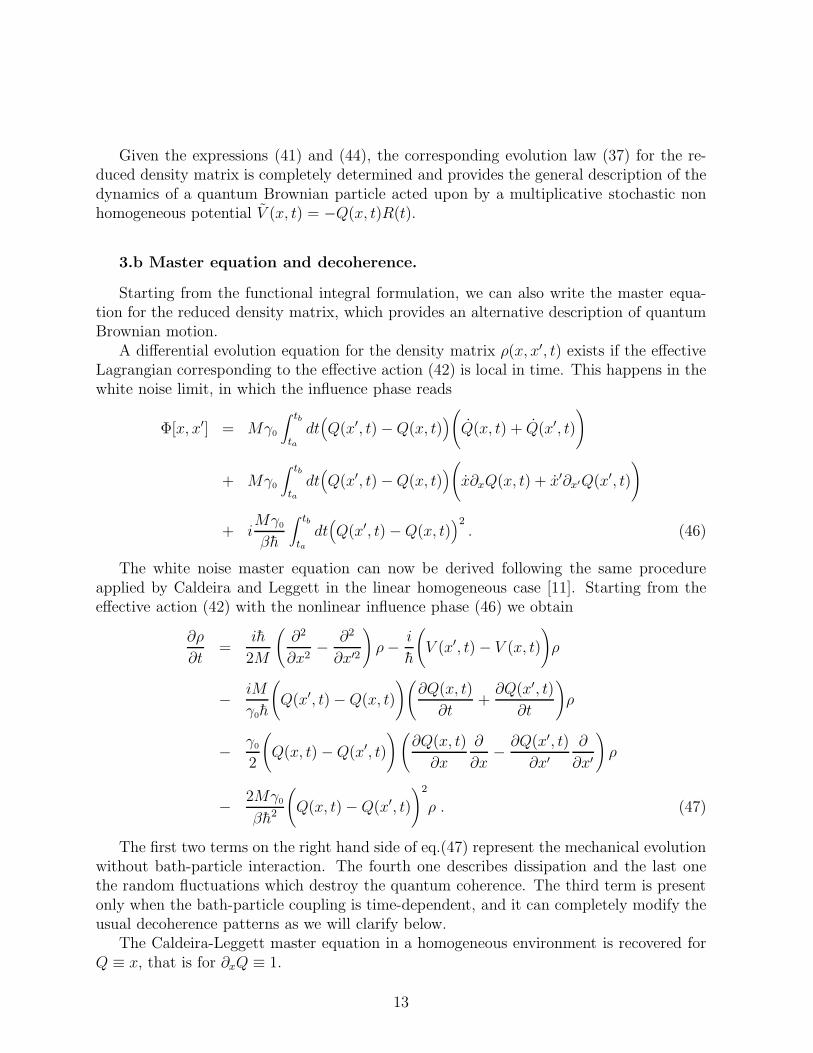
A differential evolution equation for the density matrix ρ(x, x′, t) exists if the effectiveLagrangian corresponding to the effective action (42) is local in time. This happens in thewhite noise limit, in which the influence phase reads

Φ[x, x′] = Mγ0

∫ tb

tadt(

Q(x′, t) − Q(x, t))

(

Q(x, t) + Q(x′, t)

)

+ Mγ0

∫ tb

tadt(

Q(x′, t) − Q(x, t))

(

x∂xQ(x, t) + x′∂x′Q(x′, t)

)

+ iMγ0

βh

∫ tb

tadt(

Q(x′, t) − Q(x, t))

2

. (46)

The white noise master equation can now be derived following the same procedureapplied by Caldeira and Leggett in the linear homogeneous case [11]. Starting from theeffective action (42) with the nonlinear influence phase (46) we obtain

∂ρ

∂t=

ih

2M

(

∂2

∂x2−

∂2

∂x′2

)

ρ −i

h

(

V (x′, t) − V (x, t)

)

ρ

−iM

γ0h

(

Q(x′, t) − Q(x, t)

)(

∂Q(x, t)

∂t+

∂Q(x′, t)

∂t

)

ρ

−γ0

2

(

Q(x, t) − Q(x′, t)

)(

∂Q(x, t)

∂x

∂

∂x−

∂Q(x′, t)

∂x′

∂

∂x′

)

ρ

−2Mγ0

βh2

(

Q(x, t) − Q(x′, t)

)

2

ρ . (47)

The first two terms on the right hand side of eq.(47) represent the mechanical evolutionwithout bath-particle interaction. The fourth one describes dissipation and the last onethe random fluctuations which destroy the quantum coherence. The third term is presentonly when the bath-particle coupling is time-dependent, and it can completely modify theusual decoherence patterns as we will clarify below.

The Caldeira-Leggett master equation in a homogeneous environment is recovered forQ ≡ x, that is for ∂xQ ≡ 1.

13

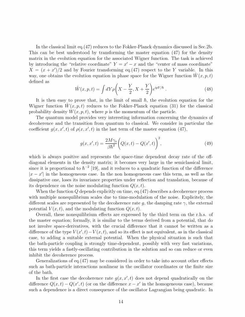
In the classical limit eq.(47) reduces to the Fokker-Planck dynamics discussed in Sec.2b.This can be best understood by transforming the master equation (47) for the densitymatrix in the evolution equation for the associated Wigner function. The task is achievedby introducing the “relative coordinate” Y = x′ − x and the “center of mass coordinate”X = (x + x′)/2 and by Fourier transforming eq.(47) respect to the Y variable. In thisway, one obtains the evolution equation in phase space for the Wigner function W (x, p, t)defined as

W (x, p, t) =∫

dY ρ

(

X −Y

2, X +

Y

2

)

eipY/h . (48)

It is then easy to prove that, in the limit of small h, the evolution equation for theWigner function W (x, p, t) reduces to the Fokker-Planck equation (31) for the classicalprobability density W (x, p, t), where p is the momentum of the particle.

The quantum model provides very interesting information concerning the dynamics ofdecoherence and the transition from quantum to classical. We consider in particular thecoefficient g(x, x′, t) of ρ(x, x′, t) in the last term of the master equation (47),

g(x, x′, t) =2Mγ0

βh2

(

Q(x, t) − Q(x′, t)

)

2

, (49)

which is always positive and represents the space-time dependent decay rate of the off-diagonal elements in the density matrix; it becomes very large in the semiclassical limit,since it is proportional to h−2 [19], and it reduces to a quadratic function of the difference|x − x′| in the homogeneous case. In the non homogeneous case this term, as well as thedissipative one, loses its invariance properties under reflection and translation, because ofits dependence on the noise modulating function Q(x, t).

When the function Q depends explicitly on time, eq.(47) describes a decoherence processwith multiple nonequilibrium scales due to time-modulation of the noise. Explicitely, thedifferent scales are represented by the decoherence rate g, the damping rate γ, the externalpotential V (x, t), and the modulating function Q(x, t).

Overall, these nonequilibrium effects are expressed by the third term on the r.h.s. ofthe master equation; formally, it is similar to the terms derived from a potential, that donot involve space-derivatives, with the crucial difference that it cannot be written as adifference of the type V (x′, t)−V (x, t), and so its effect is not equivalent, as in the classicalcase, to adding a suitable external potential. When the physical situation is such thatthe bath-particle coupling is strongly time-dependent, possibly with very fast variations,this term yields a fastly-oscillating contribution in the solution and so can reduce or eveninhibit the decoherence process.

Generalizations of eq.(47) may be considered in order to take into account other effectssuch as bath-particle interactions nonlinear in the oscillator coordinates or the finite sizeof the bath.

In the first case the decoherence rate g(x, x′, t) does not depend quadratically on thedifference Q(x, t)−Q(x′, t) (or on the difference x− x′ in the homogeneous case), becausesuch a dependence is a direct consequence of the oscillator Lagrangian being quadratic. In

14

the second case quantum interference is suppressed only as long as the system is confinedinside the thermal bath, which is assumed to possess a finite scale ξ, of the order of itslinear dimensions.

The variable Y = x−x′ is conjugate to the variable p (see the definition of the Wignerfunction) which in the semiclassical limit reduces to the momentum variable, and actuallyrepresents the quantum uncertainty on the position of the Brownian particle [20]. We thenexpect expression (48) to be replaced by a function g(x, x′, t) which becomes negligible for|x − x′| ≫ ξ.

A finite value of (48) for |x − x′| ≫ ξ, both in the homogeneous and in the nonhomogeneous models, is possible only if the bath is assumed to be infinitely extended.This point clarifies some questions recently raised [21] concerning the decoherence process.

In this paper we generalized the homogeneous model of classical and quantum dissipa-tion in order to include general bath-particle interactions nonlinear in the particle coordi-nates. The linear-dissipation theory emerges as a particular case of the model. Moreover,we have shown that the nonlinear bath-particle coupling leads to the appearance of nonhomogeneous random and dissipative forces and of a further deterministic time-dependentforce, in the Langevin equation at the classical level, and in the master equation for thequantum case. We illustrated how this yields new interesting consequences both in theclassical and in the quantum regime.

15

References

[1] N.G. Van Kampen, Stochastic Processes in Physics and Chemistry (Elsevier, Amster-dam, 1981).

[2] R.P. Feynman and F.L. Vernon, Ann. Phys. (N.Y.) 24 (1963) 118; R.P. Feynman andA.R. Hibbs, Quantum Mechanics and Path Integrals (McGraw-Hill, New York, 1965).

[3] G.W. Ford, M. Kac, and P. Mazur, J. Math. Phys. 6 (1965) 504.

[4] P. Ullersma, Physica 32 (1966) 27.

[5] R. Kubo, Progr. Theor. Phys. 29 (1965) 255; H. Mori, Progr. Theor. Phys. 33 (1965)423; M. Toda, R. Kubo, and V. Saito, Statistical Physics, Vol. II (Springer Verlag,Berlin, 1983).

[6] H. Grabert et al., Phys. Rep. 168 (1988) 115.

[7] R. Zwanzig, J. Stat. Phys. 9 (1973) 215.

[8] V. Hakim and V. Ambegaokar, Phys. Rev. A 32 (1985) 423.

[9] G.W. Ford and M. Kac, J. Stat. Phys. 46 (1987) 803.

[10] P. Schramm and H. Grabert, J. Stat. Phys. 49 (1987) 767.

[11] A.O. Caldeira and A.J. Leggett, Physica A 121 (1983) 115.

[12] W. Eckhardt, Physica A 141 (1987) 81.

[13] B.L. Hu, J.P. Paz, and Y. Zhang, Phys. Rev. D 45 (1992) 2843.

[14] C.R. Doering and J.C. Gadoua, Phys. Rev. Lett. 69 (1992) 318.

[15] R.L. Stratonovich, Topics in the Theory of Random Noise, Vol. II (Gordon andBreach, New York, 1981).

[16] K. Mohring and U. Smilansky, Nucl. Phys. A 338 (1980) 227; H. Metiu and G. Schon,Phys. Rev. Lett. 53 (1984) 13; A.O. Caldeira and A. J. Legget, Ann. Phys. (N.Y.)149 (1983) 374.

[17] K. Lindenberg and V. Seshadri, Physica A 109 (1981) 483; K. Lindenberg and B.J.West, The Nonequilibrium Statistical Mechanics of Open and Closed Systems (VCH,New York, 1990).

[18] M. Patriarca, Ph.D. Thesis, University of Perugia, 1993.

[19] W.H. Zurek, Progr. Theor. Phys. 89 (1993) 281.

16

[20] A. Schmidt, J. Low Temp. 49 (1982) 609.

[21] M.R. Gallis and G.N. Fleming, Phys. Rev. A 42 (1990) 38; M.R. Gallis, Phys. Rev.A 45 (1992) 47; Phys. Rev. A 48 (1993) 1028.

17