Aeration and Energy Dissipation over Stepped Gabion Spillways
173
THE UNIVERSITY OF QUEENSLAND REPORT CH92/13 AUTHORS: Davide WUTHRICH and Hubert CHANSON AERATION AND ENERGY DISSIPATION OVER STEPPED GABION SPILLWAYS: A PHYSICAL STUDY SCHOOL OF CIVIL ENGINEERING
-
Upload
khangminh22 -
Category
Documents
-
view
3 -
download
0
Transcript of Aeration and Energy Dissipation over Stepped Gabion Spillways
THE UNIVERSITY OF QUEENSLAND
REPORT CH92/13
AUTHORS: Davide WUTHRICH and Hubert CHANSON
AERATION AND ENERGY DISSIPATION OVER STEPPED GABION SPILLWAYS: A PHYSICAL STUDY
SCHOOL OF CIVIL ENGINEERING
HYDRAULIC MODEL REPORTS This report is published by the School of Civil Engineering at the University of Queensland. Lists of recently-published titles of this series and of other publications are provided at the end of this report. Requests for copies of any of these documents should be addressed to the Civil Engineering Secretary. The interpretation and opinions expressed herein are solely those of the author(s). Considerable care has been taken to ensure accuracy of the material presented. Nevertheless, responsibility for the use of this material rests with the user. School of Civil Engineering The University of Queensland Brisbane QLD 4072 AUSTRALIA Telephone: (61 7) 3365 4163 Fax: (61 7) 3365 4599 URL: http://www.eng.uq.edu.au/civil/ First published in 2014 by School of Civil Engineering The University of Queensland, Brisbane QLD 4072, Australia © Wuthrich and Chanson This book is copyright ISBN No. 9781742720944 The University of Queensland, St Lucia QLD, Australia
Aeration and Energy Dissipation over Stepped Gabion Spillways: a Physical Study
by
Davide WUTHRICH
Visiting research fellow, The University of Queensland, School of Civil Engineering, Brisbane
QLD 4072, Australia
Masters student, Ecole Polytechique Fédérale de Lausanne, Lausanne, Switzerland
and
Hubert CHANSON
Professor, The University of Queensland, School of Civil Engineering, Brisbane QLD 4072,
Australia, Email: [email protected]
REPORT No. CH92/13
ISBN 9781742720944
School of Civil Engineering, The University of Queensland
February 2014
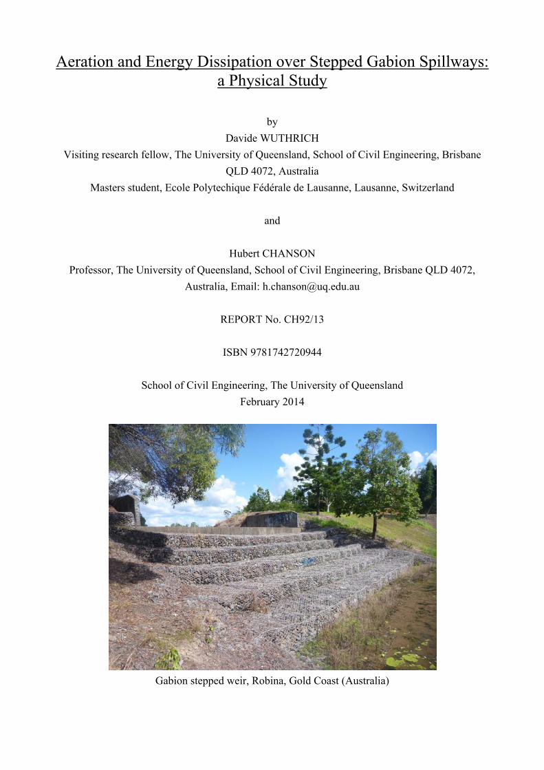
Gabion stepped weir, Robina, Gold Coast (Australia)
ii
ABSTRACT
Stepped spillway structures have been used for more than 3,000 years. Recently the design of
stepped chutes regained some interest because of their suitability with roller compacted concrete
(RCC) construction methods and gabion placement. In this study, the hydraulic performances of
gabion stepped weirs were investigated experimentally in terms of the air-water flow properties,
energy dissipation and re-oxygenation rate. A physical study was performed in a relatively large
size facility with a 26.6° slope (1V:2H) and 0.10 m step height. Three gabion stepped
configurations were tested, as well as a flat impervious stepped configuration. For each
configuration, the detailed flow properties were investigated for a wide range of discharges. Some
visual observations highlighted the seepage flow through the gabions. The seepage flow motion
resulted into a modification of the cavity flow dynamics, as well as some air bubbles were
entrapped in the gabions. The air-water flow properties showed that the air concentration, bubble
count rate and turbulent intensity profiles presented lower quantitative values in the gabion stepped
configuration, compared to those on the impervious stepped chute. In skimming flows, higher
velocities were measured at the downstream end of the gabion stepped chute, associated with
smaller energy dissipation rates and lower friction factors. The aeration performances of the gabion
stepped configurations were lesser than on the impervious stepped chute, but for low discharges,
i.e., the nappe flow regime. For two configurations, some step capping was added, and the resulting
flow properties were close to those on the impervious stepped configuration.
Keywords: Stepped spillways, Gabion stepped weirs, Air entrainment, Energy dissipation, Re-
oxygenation, Physical modelling, Air-water flow properties, Seepage flow, Impervious step
capping.

iii
TABLE OF CONTENTS
Page
Abstract ii
Keywords ii
Table of contents iii
List of symbols v
1. Introduction 1
2. Experimental facility and instrumentation 4
2.1 Presentation
2.2 Experimental facility
2.3 Instrumentation
2.4 Experimental flow conditions
3. Flow patterns 11
3.1 Basic flow patterns
3.2 Air entrainment within the gabions
3.3 Inception point of free surface aeration
4. Air -water flow properties 20
4.1 Presentation
4.2 Flat and gabion stepped configuration
4.3 Capped and fully-capped stepped configurations
4.4 Discussion
5. Energy dissipation and flow resistance 36
5.1 Residual head and energy dissipation
5.2 Flow resistance
5.3 Discussion
6. Interfacial area and mass transfer rate 41
6.1 Presentation
6.2 Mass transfer rate
6.3 Discussion
7. Conclusion 46
iv
8. Acknowledgements 48
APPENDICES
Appendix A - Photographs of stepped spillways configuration and flow patterns A-1
Appendix B - Signal processing and sensitivity analysis B-1
Appendix C - Hydraulic conductivity tests C-1
Appendix D - Air-water flow properties on flat impervious stepped configuration D-1
Appendix E - Air-water flow properties on gabion stepped configuration E-1
Appendix F - Air-water flow properties on capped stepped configuration F-1
Appendix G - Air-water flow properties on fully-capped stepped configuration G-1
Appendix H - Longitudinal distribution of characteristic air-water properties H-1
Appendix I - Video movies of air bubble motion inside the gabions I-1
REFERENCES R-1
Bibliography R-5
Internet bibliography R-6
Bibliographic reference of the Report CH92/13 R-7
v
LIST OF SYMBOLS
The following symbols are used in this report:
A gas-liquid interface area (m2);
Aw flow cross-section area (m2);
a specific interface area, defined as the air-water surface area per unit volume of air and
water (m-1);
amax maximum value of specific interface area in a cross section (m-1);
amean mean specific interface area in a cross section (m-1):
90Y
0y90mean dya
Y
1a
b characteristic value of maximum variation of β;
C void fraction or air concentration, defined as the volume of air per unit volume;
CDS concentration of dissolved gas in the downstream cross-section (kg/m3);
CFmax void fraction for which F = Fmax;
Cgas concentration of the gas dissolved in water (kg/m3);
Cmean depth-averaged void fraction defined in terms of Y90: Cmean = 1-d/Y90;
CSAT gas saturation concentration in water (kg/m3);
CUS concentration of dissolved gas in the upstream cross-section (kg/m3);
DH hydraulic diameter (m) defined as DH = 4×Aw/Pw;
Dgas molecular diffusion coefficient of the gas in water (m2/s);
Do constant function of the mean void fraction in the advective diffusion equation
(skimming flow);
d equivalent clear water flow depth (m) defined as
90Y
0y
dy)C1(d
dc critical flow depth (m);
d50 median grain size (m);
E aeration efficiency, defined as:
USSAT
USDS
CC
CCE
F bubble count rate (Hz) defined as the number of detected air bubbles per unit time;
F* Froude number defined in terms of the step cavity roughness;
Fmax maximum value of bubble count rate in a cross section (Hz);
fe equivalent Darcy-Weisbach friction factor of the air-water flow;
g gravity constant (m/s2): g = 9.794 m/s2 in Brisbane (Australia);
H (a) total head (m);
(b) piezometric head (m);
Hdam weir height (m);
Hmax upstream total head (m): Hmax = Hdam + H1 Hdam + 3/2×dc;

vi
Hres residual head of the flow (m);
H0 height (m) of the vertical seepage face on the downstream face of the gabions;
H1 reservoir elevation (m) above the spillway crest;
h vertical step height (m);
i integer;
K hydraulic conductivity of a porous medium (m/s);
Ke modified hydraulic conductivity (m/s);
KL mass transfer coefficient or liquid film coefficient (m/s);
K' integration constant in the advective diffusion equation (skimming flow);
K" integration constant in the advective diffusion equation (transition flow);
ks cavity height perpendicular to the direction of the flow (m): ks = h×cos;
ks' step surface roughness height (m);
Lo length of the horizontal seepage above the first gabion (m);
Lb distance (m) between step edge 10 and the measurement location in the bottom channel;
Lcrest length of the broad-crested weir (m);
LI longitudinal distance (m) between the inception point of aeration and step edge 1;
(LI)cavity longitudinal distance (m) between the inception point of step cavity aeration and step
edge 1;
(LI)fs longitudinal distance (m) between the inception point of free-surface aeration and step
edge 1;
(LI)gabion longitudinal distance (m) between the inception point of gabion aeration and step edge
1;
l horizontal step length (m);
Mgas mass of dissolved gas (kg);
N power law exponent;
Po porosity;
Pw wetted perimeter (m);
Q water discharge (m3/s);
q water discharge per unit width (m2/s), defined as q = Q/W;
qw water discharge per unit width (m2/s) calculated from the integration of the void ratio
and velocity profiles:
90Y
0y
w dyV)C1(q
R normalised correlation coefficient;
rcrest radius of the upstream rounded corner of the broad-crested weir (m);
Re Reynolds number defined in terms of the hydraulic diameter: Re = w×V×DH/w;
ReP Reynolds number defined in terms of the seepage flow velocity: ReP = w×uD×d50/w;
Rxx normalised auto-correlation function;
Rxy normalised cross-correlation function;
vii
Sf friction slope defined as Sf = - ∂H/∂x;
T time (s) at which the cross correlation between the probe tip signals is maximum;
TK temperature (K);
T0.5 time (s) for which the auto-correlation function Rxx(T0.5) = 0.5;
Tu turbulent intensity: Tu = u'/V;
Tumax maximum turbulent intensity in a cross section;
t time (s);
Uw mean flow velocity (m/s) defined as Uw = q/d;
uD seepage velocity (m/s);
u' root mean square of velocity fluctuations (m/s);
V interfacial velocity (m/s);
V90 characteristic interfacial velocity (m/s) where C = 0.9;
Vc critical velocity of the flow (m/s) defined as: Vc = (g×dc)1/2;
W width of the stepped spillway (m);
x longitudinal distance (m) measured along the pseudo-bottom formed by the step edges;
Y90 characteristic depth (m) where C = 0.9;
y distance (m) measured perpendicular to the pseudo-bottom formed by the step edges;
z transverse distance from the channel centreline (m);
α correction factor, function of the local void ration and flow conditions;
β correction factor, function of the local void ration and flow conditions;
ΔH total energy loss (m) defined as ΔH = Hmax - Hres ;
Δx streamwise distance between the probe tips (m);
Δz transverse distance between the probe tips (m);
Δzo difference in height between the weir crest and calculated step edge (m);
κ intrinsic permeability (m2) of the porous medium;
ν kinematic viscosity of water (m2/s): = w/w.
θ chute slope: tan = h/l;
λ dimensionless function of the mean air concentration (transition flow);
λa characteristic air bubble chord (m);
λb characteristic water chord (m);
w dynamic viscosity of water (Pa.s);
w water density (kg/m3);
surface tension between air and water (N/m);
τo boundary shear stress (Pa);
τ0.5 time for which the cross-correlation function is half of its maximum value (s);
Ø diameter of the probe sensor (m);
Subscript
c critical flow conditions;
viii
DS downstream flow conditions;
US upstream flow conditions;
90 flow properties at the characteristic location where C = 0.90;
Abbreviations
NA nappe flow regime;
PR porous seepage flow regime;
SK skimming flow regime;
TRA transition flow regime.
1
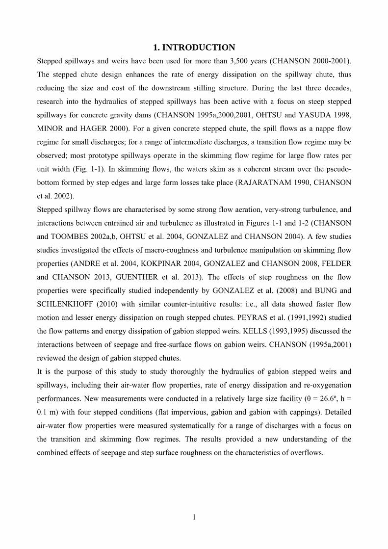
1. INTRODUCTION
Stepped spillways and weirs have been used for more than 3,500 years (CHANSON 2000-2001).
The stepped chute design enhances the rate of energy dissipation on the spillway chute, thus
reducing the size and cost of the downstream stilling structure. During the last three decades,
research into the hydraulics of stepped spillways has been active with a focus on steep stepped
spillways for concrete gravity dams (CHANSON 1995a,2000,2001, OHTSU and YASUDA 1998,
MINOR and HAGER 2000). For a given concrete stepped chute, the spill flows as a nappe flow
regime for small discharges; for a range of intermediate discharges, a transition flow regime may be
observed; most prototype spillways operate in the skimming flow regime for large flow rates per
unit width (Fig. 1-1). In skimming flows, the waters skim as a coherent stream over the pseudo-
bottom formed by step edges and large form losses take place (RAJARATNAM 1990, CHANSON
et al. 2002).
Stepped spillway flows are characterised by some strong flow aeration, very-strong turbulence, and
interactions between entrained air and turbulence as illustrated in Figures 1-1 and 1-2 (CHANSON
and TOOMBES 2002a,b, OHTSU et al. 2004, GONZALEZ and CHANSON 2004). A few studies
studies investigated the effects of macro-roughness and turbulence manipulation on skimming flow
properties (ANDRE et al. 2004, KOKPINAR 2004, GONZALEZ and CHANSON 2008, FELDER
and CHANSON 2013, GUENTHER et al. 2013). The effects of step roughness on the flow
properties were specifically studied independently by GONZALEZ et al. (2008) and BUNG and
SCHLENKHOFF (2010) with similar counter-intuitive results: i.e., all data showed faster flow
motion and lesser energy dissipation on rough stepped chutes. PEYRAS et al. (1991,1992) studied
the flow patterns and energy dissipation of gabion stepped weirs. KELLS (1993,1995) discussed the
interactions between of seepage and free-surface flows on gabion weirs. CHANSON (1995a,2001)
reviewed the design of gabion stepped chutes.
It is the purpose of this study to study thoroughly the hydraulics of gabion stepped weirs and
spillways, including their air-water flow properties, rate of energy dissipation and re-oxygenation
performances. New measurements were conducted in a relatively large size facility (θ = 26.6º, h =
0.1 m) with four stepped conditions (flat impervious, gabion and gabion with cappings). Detailed
air-water flow properties were measured systematically for a range of discharges with a focus on
the transition and skimming flow regimes. The results provided a new understanding of the
combined effects of seepage and step surface roughness on the characteristics of overflows.

2
(A) Paradise dam stepped spillway (Australia) in operation on 5 March 2013 (shutter speed: 1/1,600
s) - Flow conditions: q = 7.4 m2/s, dc/h = 2.9, skimming flow - Spillway geometry: = 57.4, h =
0.62 m, RCC dam
(B) Hinze dam stepped spillway (Australia) in operation on 29 January 2013 (shutter speed: 1/8,000
s) - Flow conditions: q = 14 m2/s, dc/h = 2.3, skimming flow - Spillway geometry: = 51.3, h = 1.2
m, Rockfill dam wall with conventional concrete spillway
Fig. 1-1 - Photographs of concrete stepped spillways in operation
3
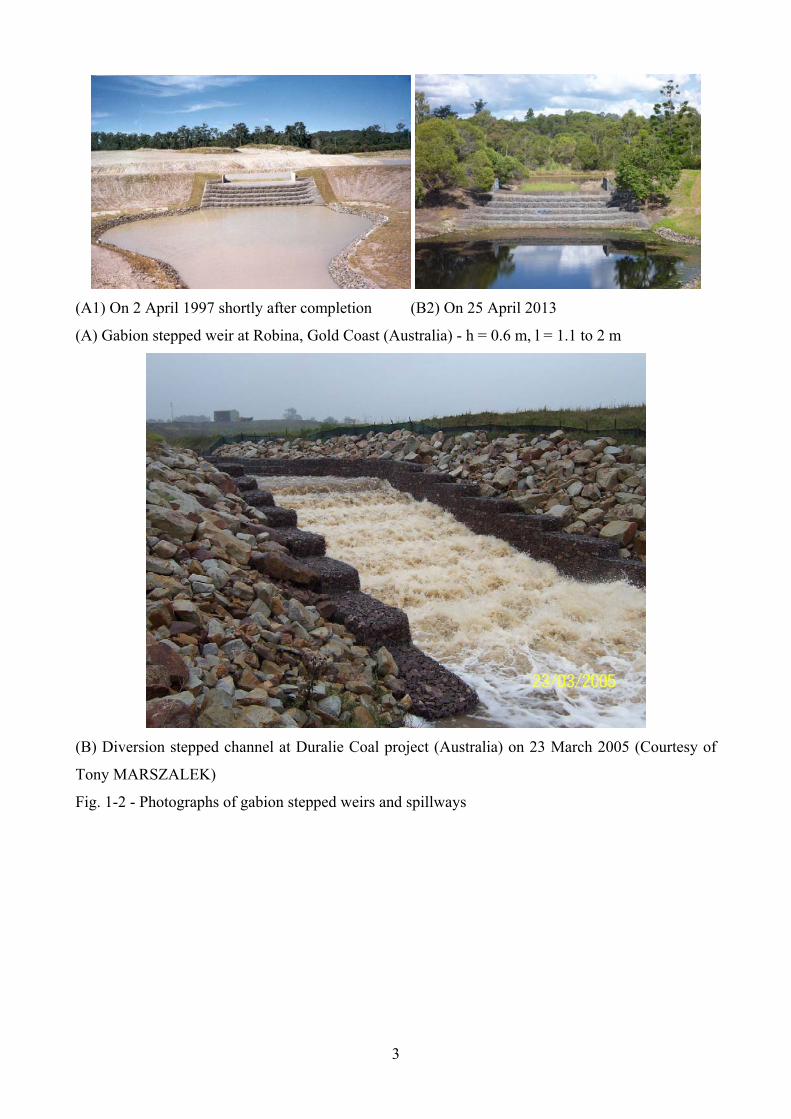
(A1) On 2 April 1997 shortly after completion (B2) On 25 April 2013
(A) Gabion stepped weir at Robina, Gold Coast (Australia) - h = 0.6 m, l = 1.1 to 2 m
(B) Diversion stepped channel at Duralie Coal project (Australia) on 23 March 2005 (Courtesy of
Tony MARSZALEK)
Fig. 1-2 - Photographs of gabion stepped weirs and spillways
4
2. EXPERIMENTAL FACILITY AND INSTRUMENTATION
2.1 PRESENTATION
Physical hydraulic models are commonly used during the design stages to optimise a spillway and
to ensure a safe operation of the structure. In a physical model, the flow conditions must be similar
to those in the prototype: that is, a similarity of form, of motion and of forces. In free-surface flows,
a Froude similitude is typically applied to scale the flow motion. In most applications, the physical
hydraulic model is a smaller-size representation of the prototype; thus scale effects might take
place.
For a rectangular gabion stepped weir, a simplified dimensional analysis leads to a number of
relationships between the air-water (over)flow properties, fluid properties, boundary conditions and
channel geometries:
,....Po,d
'k,,
d
W,
g,
DV,
h
d,
d
z,
d
y,
d
xF,...da,
V
dF,
V
'u,
V
V,C
c
s
c3
w
4w
w
Hw
c
ccc1c
c
c
cc
(2-1)
where C is the void fraction, V is the interfacial velocity, u' is a characteristic velocity fluctuation, F
is the bubble count rate, a is the specific interface area, dc and Vc are the critical flow depth and
velocity respectively, x, y, z are respectively the longitudinal, normal and transverse coordinates,
DH is the hydraulic diameter, W is the channel width, h and l are the step height and length
respectively, g is the gravity acceleration, θ is the chute slope, μw is the dynamic viscosity of water,
ρw is the water density, σ is the surface tension between air and water, ks' is the equivalent sand
roughness height of the step boundary surface, Po is the gabion porosity. Equation (2-1) expresses
the dimensionless air-water overflow properties at a location (x,y,z) as functions of the relevant
dimensionless parameters, including Froude, Reynolds and Morton numbers. Indeed the
dimensionless discharge dc/h is proportional to a Froude number defined in terms of the step height:
3/23c )hg/q(h/d where q is the water discharge per unit width. Note that the grain size and
mesh characteristics are implicitly accounted for by the equivalent sand roughness height ks'.
In the present study, the Morton number was an invariant because the same fluids were used in
model and prototype (WOOD 1991, CHANSON 2009, PFISTER and CHANSON 2012). Similarly,
the chute slope (tan = h/l) and the channel width W were kept constant during the experimental
study, while all the measurements were conducted on the channel centreline. Hence Equation (2-1)
may be simplified into:
,....Po,d
'k,
DV,
h
d,
d
y,
d
xF,...da,
V
dF,
V
'u,
V
V,C
c
s
w
Hw
c
cc2c
c
c
cc
(2-2)
Herein a Froude similitude was developed and the experiments were conducted in a large size
facility which operated at large Reynolds numbers (Table 2-1, column 4) with relatively large-size

5
gabion material. These conditions may correspond to a 1:3 to 1:6 scale study of the gabion stepped
weirs shown in Figure 1-2, thus ensuring that the extrapolation of the laboratory data to prototype
conditions is unlikely to be adversely affected by scale effects.
2.2 EXPERIMENTAL FACILITY
New experiments were conducted in a relatively large size stepped spillway model at the University
of Queensland. The facility was previously used by FELDER and CHANSON (2013a,b) and
GUENTHER et al. (2013). The test section consisted of a broad-crested weir followed by ten steps
with step height h = 0.1 m and step length l = 0.2 m. The chute was 0.52 m wide.
A pump controlled with an adjustable frequency AC motor drive delivered the flow rate, allowing
an accurate discharge adjustment in a closed-circuit system. The water flow was supplied by a large
upstream intake basin followed by a smooth sidewall convergent with a 4.23:1 contraction ratio. At
the upstream end of the chute, the flow was controlled by a broad-crested weir equipped with an
upstream rounded corner. The water discharge was deduced from the measured upstream head
above crest using the discharge calibration results of FELDER and CHANSON (2012):
3
1crest
1 H3
2g
L
H153.092.0
W
Q
(2-3)
where H1 is the upstream total head above the crest and Lcrest is length of the broad-crested weir
(Lcrest = 1.01 m). At the downstream end, the stepped chute was followed by a smooth horizontal
channel ending with an overfall. The flow was supercritical in this horizontal tailwater raceway for
all investigated flow conditions (Table 2-1).
Four stepped configurations were tested (Fig. 2-1). The flat impervious stepped configuration
consisted of smooth impervious steps made of marine ply. For the other three configurations, ten
identical gabions were installed above the smooth impervious steps. Each gabion was 0.3 m long,
0.1 high and 0.52 m wide, made of fine 12.7×12.7 mm2 galvanised metallic mesh and filled with
natural river pebbles (Fig. 2-2). The gravels (Cowra pearl) were sieved with 14 mm square sieve.
The density of the dry gravels was 1.6 tonnes/m3 corresponding to a porosity Po 0.35-0.4. The
hydraulic conductivity of the gabions was estimated to be K 10-1 m/s. Full details of the hydraulic
conductivity tests are presented in Appendix C. Note that the ratio of stone size to mesh size was
typical of construction practices for more economical cage filling and better adaptability of gabions
to deformation (AGOSTINI et al. 1987, CHANSON 2001).
The capped stepped configuration was obtained by installing 6 mm thick plexiglass plates on the
horizontal faces of steps 2 to 10. Each plexiglass plate was 0.195 m long and 0.51 m wide. All the
step edges were identically shaped, with the plate sharp edge ending 6-7 mm before the gabion

6
edge. The first horizontal step was not capped, allowing water to seep directly into the first gabion
(Fig. 2-1C). The fully-capped stepped configuration was identical to the capped one, but for the
addition of a plexiglass plate covering both the crest of the weir and first gabion (Fig. 2-1D).
Table 2-1 - Experimental investigations of air-water flow properties on stepped spillways
Reference θ (°) Geometry Flow conditions Instrumentation
(1) (2) (3) (4) (5)
Gabion steps (plain) Capped steps (layer cake) Upward steps
PEYRAS et. al (1991)
45 26.6 18.3
h = 0.2 m, l = 0.4 m W = 0.8 m
Pooled steps (End Sill)
Q = 0.05 - 0.2 m3/s Re = 2.5×10⁵ - 1.0×10⁶
Pitot tube array (copper pipe with inlet holes every 5 cm)
15.9 Flat steps: h = 0.1 m, l = 0.35 m W = 1 m
Q = 0.05 - 0.26 m3/s Re = 2.0×10⁵ - 1.0×10⁶
Double-tip conductivity probe (Ø = 0.025 mm).
CHANSON & TOOMBES (2002b) 21.8 Flat steps: h = 0.1 m, l = 0.25 m
W = 1 m Q = 0.04 - 0.18 m3/s Re = 1.6×10⁵ - 7.2×10⁵
Double-tip conductivity probe (Ø = 0.025 mm).
TOOMBES & CHANSON (2005)
3.4 Flat steps: h = 0.143 m, l = 2.4 m, W = 0.5 m Flat step: h = 0.143 m, W = 0.25 m
Q = 0.021 - 0.075 m3/s Re = 3×10⁵ - 6×10⁵
Single tip conductivity probe (Ø = 0.35 mm) Double tip conductivity probe (Ø = 0.025 mm)
A: rough step faces
B: rough vertical faces
C: rough horizontal faces
GONZALEZ et al. (2008)
21.8 h = 0.1 m l = 0.25 m W = 1 m
S: smooth steps
Q = 0.01 - 0.22 m3/s, Re = 5×10⁴ - 7×10⁵
Double tip conductivity probe (Ø = 0.025 mm)
TOOMBES & CHANSON (2008a,b)
3.4 Flat steps: h = 0.143 m, l = 2.4 m, W = 0.5 m Flat step: h = 0.143 m, W = 0.25 m
Q = 0.02 - 0.49 m3/s, Re = 1.6×10⁵ - 1.5×10⁶
Single tip conductivity probe (Ø = 0.35 mm) Double tip conductivity probe (Ø = 0.025 mm)
FELDER & CHANSON (2009)
21.8 Flat steps: h = 0.05 m, l = 0,125 m W = 1 m
Q = 0.04 - 0.18 m3/s Re = 1.7×10⁵ - 7.2×10⁵
Single-tip conductivity probe (Ø =0.35 mm) Double-tip conductivity probe (Ø =0.25 mm)
BUNG & SCHLENKHOFF (2010)
26.6 Flat steps: h = 0.06 m W = 0.30 m (1) Flat steps (2a) Rough horizontal faces (in row) (2b) Rough horizontal faces (shifted)
Q = 0.021, 0.027 & 0.33 m3/s Re = 2.7×10⁵, 3.6×10⁵, 4.4×10⁵
Double-tip conductivity probe (Ø =0.13 mm, Δx = 5.1 mm, Δy = 1 mm)
FELDER & CHANSON (2013b)
26.6 Flat steps : h = 0.1 m, l = 0.2 m Pooled steps: h = 0.1 m, w = 3.1 cm Porous pooled steps: h = 0.1 m, w = 3.1 cm, Po = 5 % Porous pooled steps: h = 0.1 m, w = 3.1 cm, Po = 31 % W = 0.52 m
Q = 0.013 - 0.13 m3/s Re = 1.0×10⁵ - 1.0×10⁶
Double tip conductivity probe (Ø = 0.25 mm, Δx = 7.2 mm, Δz = 2.1 mm)
Flat and impervious
Gabion and porous
Capped and porous
Present Study 26.6 h = 0.1 m l = 0.2 m W = 0.52 m
Fully-capped and porous
Q = 0.02 - 0.11 m3/s, Re = 1.4×10⁵ - 8.8×10⁵
Double tip conductivity probe (Ø = 0.25 mm, Δx = 6.2 mm, Δz = 1.35 mm)
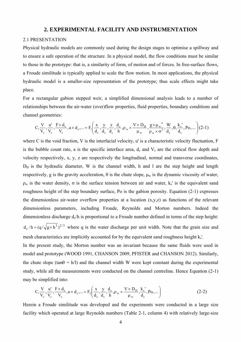
Notes: h: step height; l: step length; Q: water discharge, Re: Reynolds number defined in terms of
7
hydraulic diameter; W: width of channel; Ø: probe diameter; Δx: streamwise distance between
probe tips; Δy: vertical distance between probe tips; Δz: transverse distance between probe tips; θ:
chute slope.
(A) Flat impervious stepped configuration (dc/h = 1.3)
(B) Gabion stepped configuration (dc/h ~ 0.9)

8
(C, Left) Capped gabion configuration - Note the absence of capping on the first gabion
(D, Right) Fully-capped gabion configuration (dc/h = 0.5)
Fig. 2-1 - Photographs of the experimental configurations
Fig. 2-2 - Details of the gabion placement: view in elevation
2.3 AIR-WATER FLOW INSTRUMENTATION
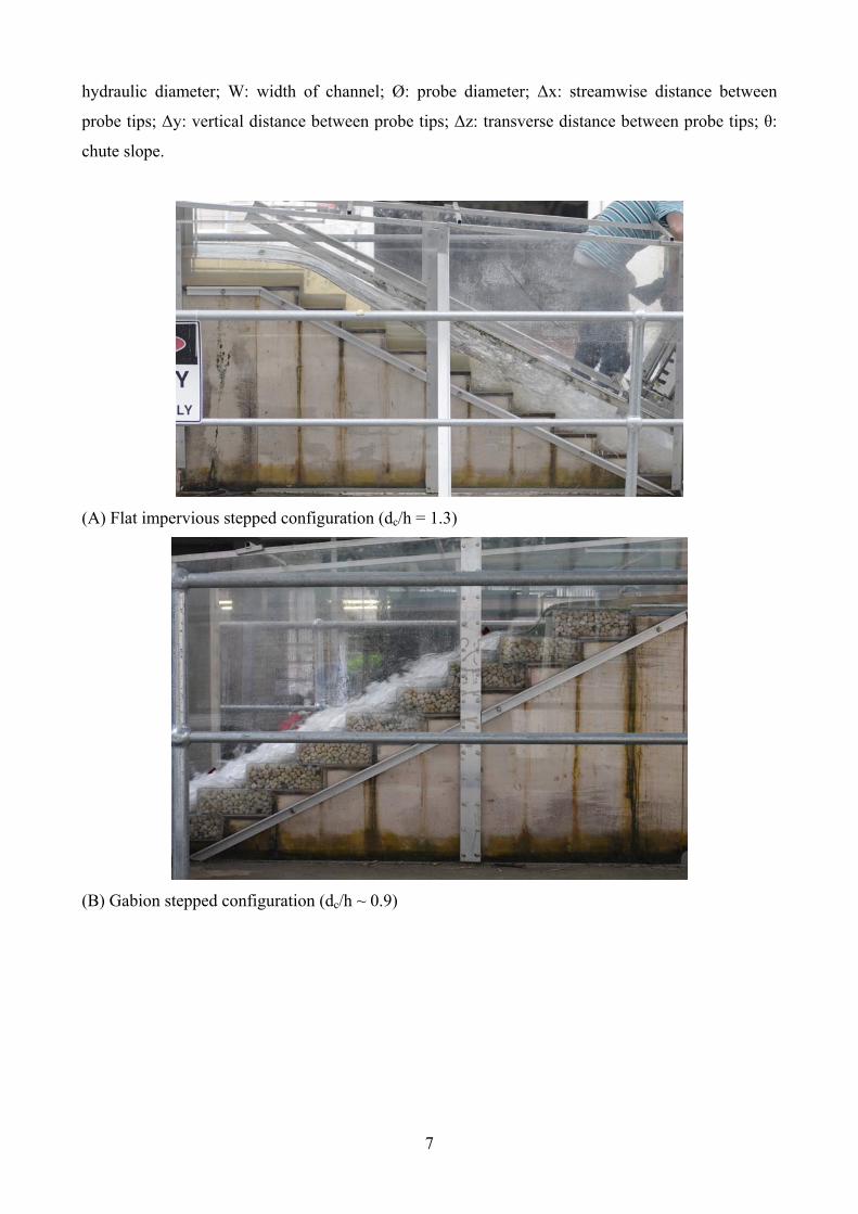
The air-water flow measurements were conducted with a phase detection intrusive probe (Fig. 2-3).
The probe was manufactured with two identical tips based upon a needle tip design. The recordings
were performed at all step edges downstream of the inception point using the double-tip
9
conductivity probe which had an inner tip diameter Ø = 0.25 mm and a separation of probe tips Δx
= 6.2 mm in the longitudinal direction (Fig. 2-3) and Δz = 1.35 mm in the transverse direction. The
conductivity probe was mounted on a trolley and the elevation in the direction perpendicular to the
pseudo bottom formed by the step edges was controlled by a fine adjustment screw-drive
mechanism equipped with a MitutoyoTM digital ruler (accuracy < 0.1 mm). Similar double-tip
conductivity probes were previously used in a number of air-water flow studies at the University of
Queensland (CAROSI and CHANSON 2008, FELDER and CHANSON 2009, GUENTHER et al.
2013).
The probe was excited by an electronic air bubble detector with a response frequency greater than
100 kHz. The probe signal output was sampled at 20 kHz per sensor for 45 seconds. The selection
of the sampling rate and duration was derived from a sensitivity analysis (Appendix B). The signals
were processed with a Fortran code developed at the University of Queensland (FELDER 2013).
The main parameters derived from the signal processing were the void fraction C, bubble frequency
F, interfacial velocity V, turbulent intensity Tu and specific interfacial area a. Further details on the
signal post-processing were discussed in CHANSON and CAROSI (2007) and CHANSON
(2002,2013).
Fig. 2-3 - Details of the dual-tip phase detection probe (shutter speed: 1/25 s) - View in elevation
with flow direction from left to right
2.4 EXPERIMENTAL FLOW CONDITIONS
The experimental study was conducted on the four stepped spillway configurations. Flow
visualisations were carried out for all configurations for a wide range of discharges within 0.005 ≤
Q ≤ 0.114 m3/s. The air-water flow properties were recorded mostly in the transition and skimming
flow regimes, for a range of dimensionless discharges between 0.5 ≤ dc/h ≤ 1.7 corresponding to
Reynolds numbers between 1.40×10⁵ and 8.78×10⁵. The experimental flow conditions are
10
summarised and compared with previous air-water flow studies in Table 2-1. They are further
detailed in Table 2-2.
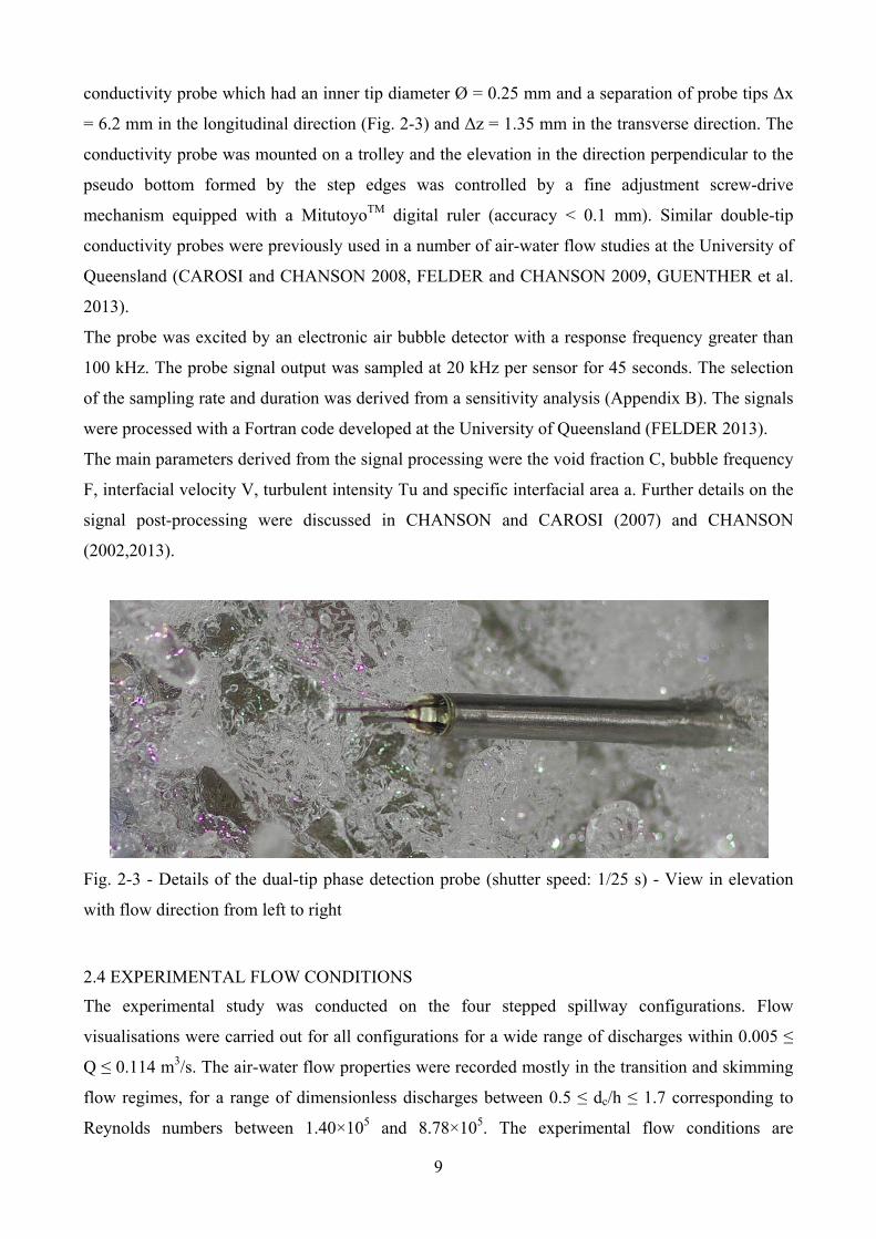
Table 2-2 - Experimental flow conditions for all stepped configurations (Present study, θ = 26.6°, h
= 0.10 m)
Configuration Q [m3/s]
dc/h [-]
Re [-]
Flow investigations
0.005 – 0.114
0.2 - 1.7 3.54104 – 8.78105
Flow observations, flow regimes
0.018 0.5 1.40×10⁵ 0.037 0.8 2.83×10⁵ 0.059 1.1 4.57×10⁵ 0.076 1.3 5.87×10⁵ 0.095 1.5 7.28×10⁵
Flat stepped configuration (h = 0.10 m θ = 26.6°)
0.114 1.7 8.78×10⁵
Measurements or air-water flow properties at all step edges
downstream of the inception point
0.005 – 0.114
0.2 - 1.7 3.54104 – 8.78105
Flow observations, flow regimes, inception point, dye study, string study
0.018 0.5 1.40×10⁵ 0.037 0.8 2.83×10⁵ 0.059 1.1 4.57×10⁵ 0.076 1.3 5.87×10⁵ 0.095 1.5 7.28×10⁵
Gabion stepped configuration (h = 0.10 m θ = 26.6°)
0.114 1.7 8.78×10⁵
Measurements or air-water flow properties at all step edges
downstream of the inception point
0.005 – 0.114
0.2 - 1.7 3.54104 – 8.78105
Flow observations, flow regimes, inception point, dye study, string study
0.018 0.5 1.40×10⁵ 0.037 0.8 2.83×10⁵ 0.059 1.1 4.57×10⁵ 0.076 1.3 5.87×10⁵ 0.095 1.5 7.28×10⁵
Capped stepped configuration (h = 0.10 m θ = 26.6°)
0.114 1.7 8.78×10⁵
Measurements or air-water flow properties at all step edges
downstream of the inception point
0.005 – 0.114
0.2 - 1.7 3.54104 – 8.78105
Flow observations, flow regimes, inception point, dye study
0.018 0.5 1.40×10⁵ 0.037 0.8 2.83×10⁵ 0.059 1.1 4.57×10⁵ 0.076 1.3 5.87×10⁵ 0.095 1.5 7.28×10⁵
Fully-capped stepped
configuration (h = 0.10 m θ = 26.6°)
0.114 1.7 8.78×10⁵
Measurements or air-water flow properties at all step edges
downstream of the inception point
11
3. FLOW PATTERNS
3.1 PRESENTATION
Visual observations were carried out for all configurations for a wide range of dimensionless
discharges dc/h up to 1.7. For all stepped configurations, the 'classical' flow regimes were identified:
namely nappe, transition and skimming flows with increasing flow rates. In addition a porous flow
regime was observed on the gabion stepped configurations for very low discharges. A summary of
flow properties of the changes between flow regimes is reported in Table 3-1. A detailed review of
flow visualisations is presented in Appendix A.
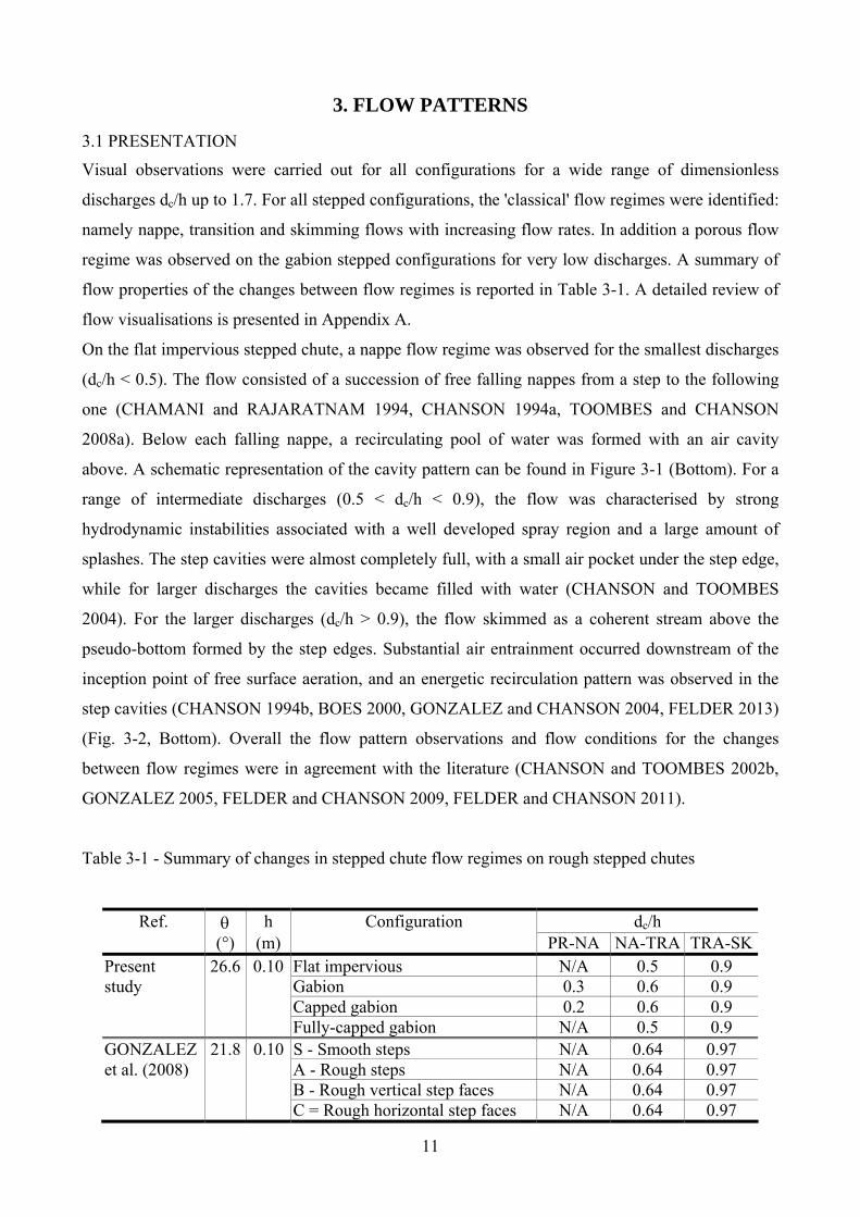
On the flat impervious stepped chute, a nappe flow regime was observed for the smallest discharges
(dc/h < 0.5). The flow consisted of a succession of free falling nappes from a step to the following
one (CHAMANI and RAJARATNAM 1994, CHANSON 1994a, TOOMBES and CHANSON
2008a). Below each falling nappe, a recirculating pool of water was formed with an air cavity
above. A schematic representation of the cavity pattern can be found in Figure 3-1 (Bottom). For a
range of intermediate discharges (0.5 < dc/h < 0.9), the flow was characterised by strong
hydrodynamic instabilities associated with a well developed spray region and a large amount of
splashes. The step cavities were almost completely full, with a small air pocket under the step edge,
while for larger discharges the cavities became filled with water (CHANSON and TOOMBES
2004). For the larger discharges (dc/h > 0.9), the flow skimmed as a coherent stream above the
pseudo-bottom formed by the step edges. Substantial air entrainment occurred downstream of the
inception point of free surface aeration, and an energetic recirculation pattern was observed in the
step cavities (CHANSON 1994b, BOES 2000, GONZALEZ and CHANSON 2004, FELDER 2013)
(Fig. 3-2, Bottom). Overall the flow pattern observations and flow conditions for the changes
between flow regimes were in agreement with the literature (CHANSON and TOOMBES 2002b,
GONZALEZ 2005, FELDER and CHANSON 2009, FELDER and CHANSON 2011).
Table 3-1 - Summary of changes in stepped chute flow regimes on rough stepped chutes
Ref. h Configuration dc/h (°) (m) PR-NA NA-TRA TRA-SK
Present 26.6 0.10 Flat impervious N/A 0.5 0.9 study Gabion 0.3 0.6 0.9 Capped gabion 0.2 0.6 0.9 Fully-capped gabion N/A 0.5 0.9 GONZALEZ 21.8 0.10 S - Smooth steps N/A 0.64 0.97 et al. (2008) A - Rough steps N/A 0.64 0.97 B - Rough vertical step faces N/A 0.64 0.97 C = Rough horizontal step faces N/A 0.64 0.97
12
Fig. 3-1 - Nappe flow regime on gabion and impervious stepped configurations: definition sketches
- From top left in the clockwise direction: gabion steps, capped gabion steps, flat impervious steps
On the gabion stepped spillway, a porous seepage flow regime was observed for very small
discharges (dc/h < 0.3). In that flow regime, all the water seeped through the gabion materials. On
the first gabion box, some infiltration was observed as shown in Figure 3-3A. A short horizontal
seepage face was observed on each step and there was no overflow past the step edges. In the
porous material, the free-surface (i.e. water table) could be observed through the transparent
sidewalls. A relatively large amount of water (i.e. the total discharge) was seen coming out of the
10th gabion box to fulfil the conservation of mass. For the smallest discharges, some vertical
seepage was not observed through the step vertical face. With increasing discharge, some small
water jets came out of the gabions as shown in Figure 3-3B. The transition between porous and
nappe flow regimes occurred once some overflow took place at the first gabion. The nappe flow
(0.3 < dc/h < 0.6) appeared as a succession of free falling nappes from one step edge to the next one
(Fig. 3-1, Top left). The cavity behind the nappe was filled with a superposition of seepage jets
coming out of the upstream gabion (Fig. 3-1, Top Left). In the lower part of the cavity an oscillating
recirculation pool was observed. The recirculation motion in the cavity pool exhibited a different

13
flow pattern compared to that observed on flat impervious stepped spillways. This is illustrated in
Figure 3-1.
Fig. 3-2 - Skimming flow regime on gabion and impervious stepped configurations: definition
sketches - From top left in the clockwise direction: gabion steps, capped gabion steps, flat
impervious steps
(A) dc/h = 0.20, Q = 0.005 m3/s, Re = 3.5104 (B) dc/h = 0.25, Q = 0.006 m3/s, Re = 4.9104
First gabion box located at end of broad-crest Steps in the middle of the staircase chute
Fig. 3-3 - Porous flow regime on the gabion stepped configuration
14
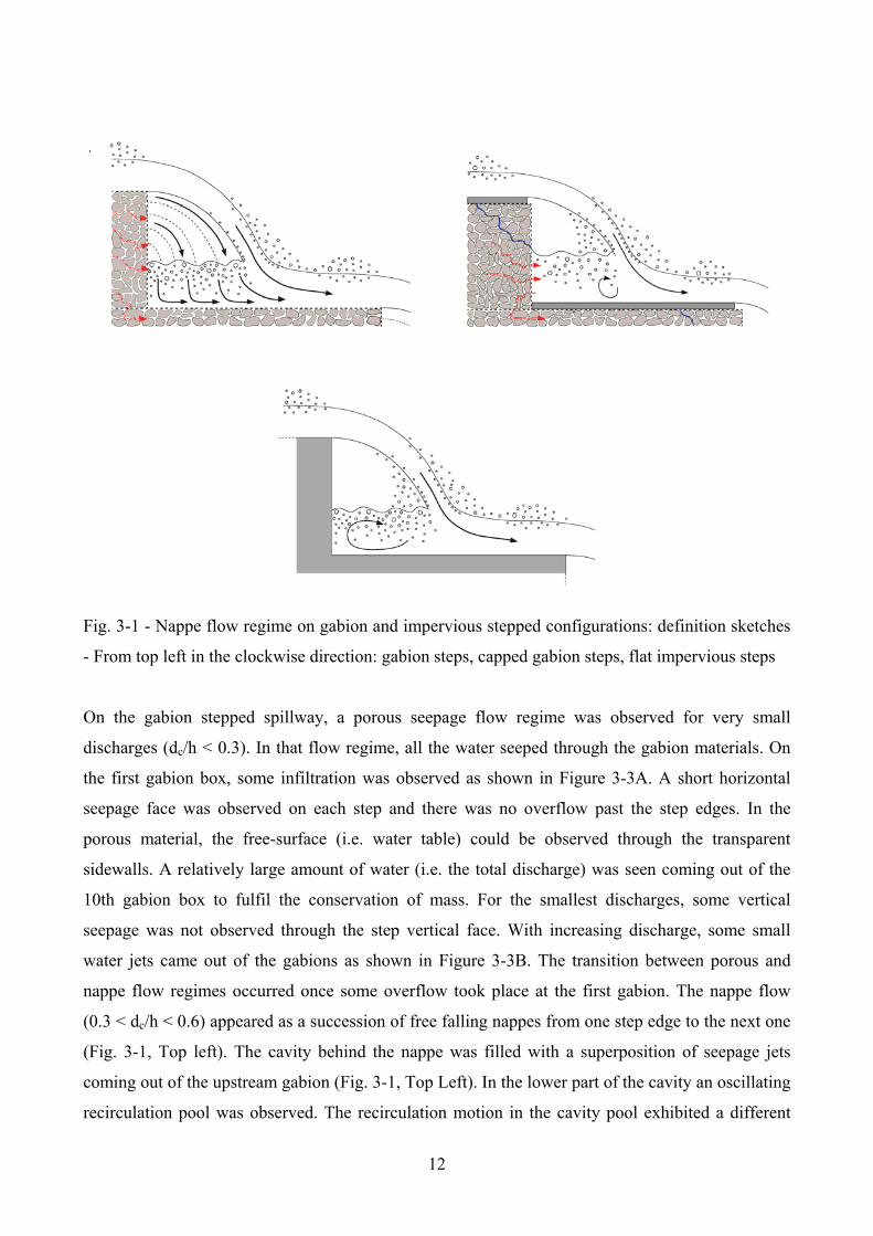
Fig. 3-4 - Cavity flow pattern in a skimming flow on gabion stepped configuration - Flow
conditions: step cavity 7-8, Q = 0.068 m3/s, dc/h = 1.20, Re = 5.2105 - Note the clear water core in
the step cavity
A transition flow regime was observed for 0.6 < dc/h < 0.9. The hydrodynamic instabilities and
splashes appeared less intense than those observed on flat impervious stepped spillways. For the
largest discharges, a skimming flow was observed (dc/h > 0.90). The flow pattern was generally
similar to that observed on the flat stepped configuration. However a different streamline pattern
was seen next to the stagnation point on the horizontal step face (Fig. 3-2, Top left). Some bubbly
flow and air bubble entrainment into the gabions were observed, mostly in the upper corner of each
gabion box downstream of the inception point of free-surface aeration. Further differences were
found in terms of cavity flow motion as a result of seepage flow effect. Detailed string studies were
carried out to visualise the cavity flow. A vertical flow of air bubbles was observed close to the
vertical step face (Fig. 3-4). In the centre of the cavity a clear water core was seen in all cavities
downstream of the inception point for all discharges. The existence of a similar clear water core was
previously reported by GONZALEZ et al. (2008) for rough impervious steps. Visually the
recirculation motion appeared to be restricted by the existence of the clear-water core. In the gabion
stepped configuration, a continuous interaction between the cavity and the gabion was noted. The
behaviour of the flow inside the cavity is schematically sketched in Figure 3-2 (Top left).
On the capped gabion stepped chute, a porous regime was observed for dc/h < 0.20. For larger
discharges, a nappe flow regime was seen for 0.20 < dc/h < 0.60, a transition flow for 0.60 < dc/h <
0.90, and the skimming flow for dc/h > 0.90. In these flow regimes (nappe, transition and skimming
15
flows), the flow patterns were similar to those observed on the flat impervious stepped chute. Some
differences were noticed at cavity level as a consequence of the seepage flow through the gabions.
This is sketched in Figure 3-1 (Top right) and Figure 3-2 (Top right). The effect of the seepage flow
was mostly noticeable for the small discharges, i.e., for the porous and nappe flow regime. The
skimming flow did not appear to be much influenced by the seepage flow.
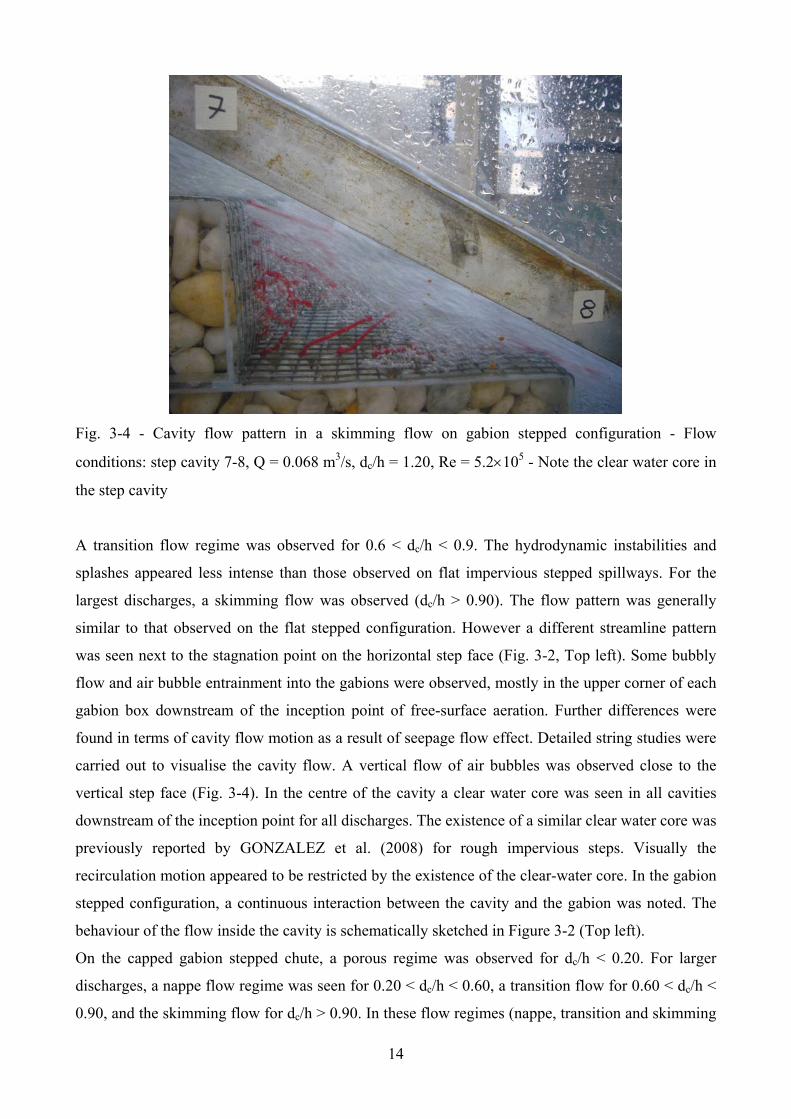
On the fully capped gabion stepped configurations, the flow patterns were generally close to those
observed on the flat impervious stepped chute and capped gabion stepped configuration, but for the
first step cavity. As illustrated in Figure 3-5, some seepage into the gabion took place through the
vertical step face beneath the first step edge.
(A) Q = 0.006 m3/s, dc/h = 0.25, Re = 4.9104 (B) Q = 0.018 m3/s, dc/h = 0.50, Re = 1.4105
Fig. 3-5 - Seepage flow visualisation on fully-capped gabion stepped configuration using dye
injection - Flow conditions in nappe flows, red dye injection (step cavity 1-2)
3.2 AIR ENTRAINMENT WITHIN THE GABIONS
A key difference between the flat impervious and gabion stepped chutes was the entrainment of air
bubbles inside the gabions. For all porous configurations, air bubbles were seen flowing through the
gravel (App. I). Appendix I regroups a series of digital video movies of bubbly flow motion in the
gabions. Visually, the bubbly flow in the gabions appeared to depend upon the water discharge,
flow regime, and step cavity location.
The largest amount of gabion bubble motion was observed in the gabion stepped structure for a
given (over)flow rate. (Lesser air entrainment in gabions was seen in the capped and fully-capped
stepped configurations for an identical flow rate.) With a nappe (over)flow regime, a large amount
of bubbles moved inside the top edge of the gabions (Fig 3-6). A majority of bubbles flowed
through the gabions and into the downstream step cavity. Some collided with gravel particles and
emerged into the cavity by buoyancy. A few bubbles flowed through the gravel into the downstream
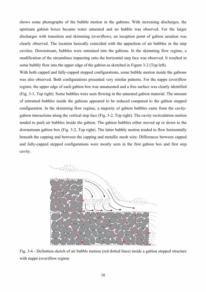
gabion box. A sketch of the bubbly flow inside the gabions is presented in Figure 3-6. Figure 3-7
16
shows some photographs of the bubble motion in the gabions. With increasing discharges, the
upstream gabion boxes became water saturated and no bubble was observed. For the larger
discharges with transition and skimming (over)flows, an inception point of gabion aeration was
clearly observed. The location basically coincided with the apparition of air bubbles in the step
cavities. Downstream, bubbles were entrained into the gabions. In the skimming flow regime, a
modification of the streamlines impacting onto the horizontal step face was observed. It resulted in
some bubbly flow into the upper edge of the gabion as sketched in Figure 3-2 (Top left).
With both capped and fully-capped stepped configurations, some bubble motion inside the gabions
was also observed. Both configurations presented very similar patterns. For the nappe (over)flow
regime, the upper edge of each gabion box was unsaturated and a free surface was clearly identified
(Fig. 3-1, Top right). Some bubbles were seen flowing in the saturated gabion material. The amount
of entrained bubbles inside the gabions appeared to be reduced compared to the gabion stepped
configuration. In the skimming flow regime, a majority of gabion bubbles came from the cavity-
gabion interactions along the vertical step face (Fig. 3-2, Top right). The cavity recirculation motion
tended to push air bubbles inside the gabion. The gabion bubbles either moved up or down to the
downstream gabion box (Fig. 3-2, Top right). The latter bubbly motion tended to flow horizontally
beneath the capping and between the capping and metallic mesh wire. Differences between capped
and fully-capped stepped configurations were mostly seen in the first gabion box and first step
cavity.
Fig. 3-6 - Definition sketch of air bubble motion (red dotted lines) inside a gabion stepped structure
with nappe (over)flow regime
17
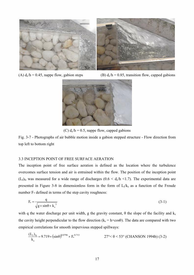
(A) dc/h = 0.45, nappe flow, gabion steps (B) dc/h = 0.85, transition flow, capped gabions
(C) dc/h = 0.5, nappe flow, capped gabions
Fig. 3-7 - Photographs of air bubble motion inside a gabion stepped structure - Flow direction from
top left to bottom right
3.3 INCEPTION POINT OF FREE SURFACE AERATION
The inception point of free surface aeration is defined as the location where the turbulence
overcomes surface tension and air is entrained within the flow. The position of the inception point
(LI)fs was measured for a wide range of discharges (0.6 < dc/h <1.7). The experimental data are
presented in Figure 3-8 in dimensionless form in the form of LI/ks as a function of the Froude
number F* defined in terms of the step cavity roughness:
3
s
*ksing
qF
(3-1)
with q the water discharge per unit width, g the gravity constant, θ the slope of the facility and ks
the cavity height perpendicular to the flow direction (ks = h×cos). The data are compared with two
empirical correlations for smooth impervious stepped spillways:
713.0*
0796.0
s
fsI Fsin719.9k
)L( 27°< θ < 53° (CHANSON 1994b) (3-2)
18
*s
fsI F11.505.1k
)L( =21.8°, 0.45 < dc/h < 1.6 (CAROSI and CHANSON 2008) (3-3)
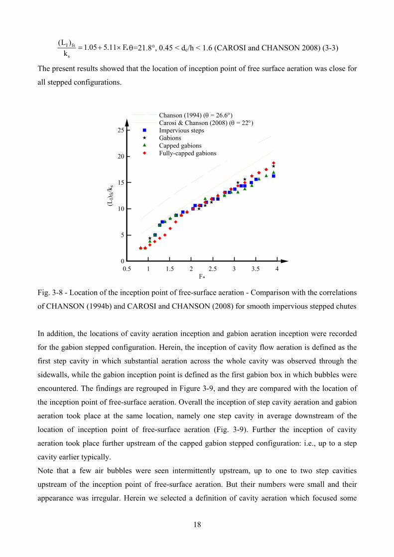
The present results showed that the location of inception point of free surface aeration was close for
all stepped configurations.
F*
(LI)
fs/k
s
0.5 1 1.5 2 2.5 3 3.5 40
5
10
15
20
25
Chanson (1994) ( = 26.6)Carosi & Chanson (2008) ( = 22)Impervious stepsGabionsCapped gabionsFully-capped gabions
Fig. 3-8 - Location of the inception point of free-surface aeration - Comparison with the correlations
of CHANSON (1994b) and CAROSI and CHANSON (2008) for smooth impervious stepped chutes
In addition, the locations of cavity aeration inception and gabion aeration inception were recorded
for the gabion stepped configuration. Herein, the inception of cavity flow aeration is defined as the
first step cavity in which substantial aeration across the whole cavity was observed through the
sidewalls, while the gabion inception point is defined as the first gabion box in which bubbles were
encountered. The findings are regrouped in Figure 3-9, and they are compared with the location of
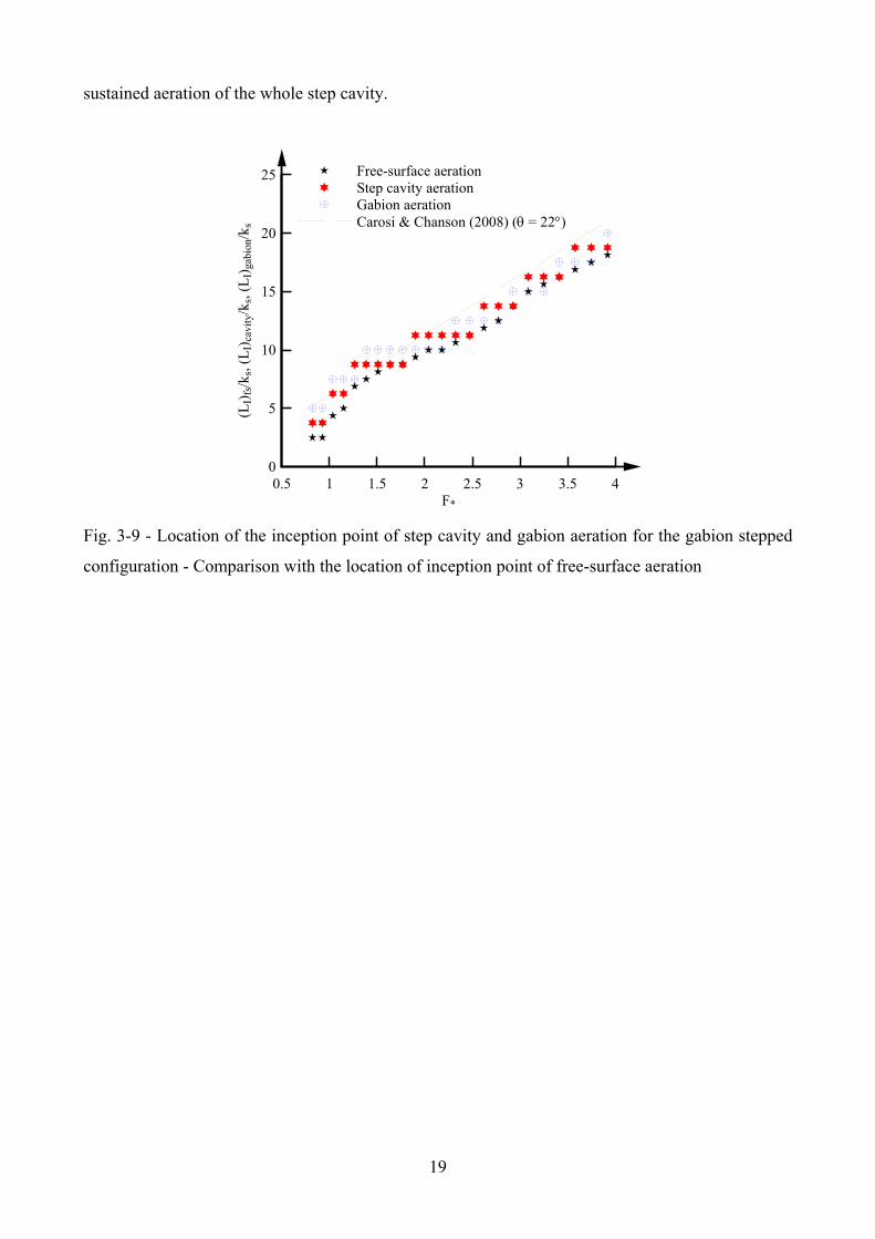
the inception point of free-surface aeration. Overall the inception of step cavity aeration and gabion
aeration took place at the same location, namely one step cavity in average downstream of the
location of inception point of free-surface aeration (Fig. 3-9). Further the inception of cavity
aeration took place further upstream of the capped gabion stepped configuration: i.e., up to a step
cavity earlier typically.
Note that a few air bubbles were seen intermittently upstream, up to one to two step cavities
upstream of the inception point of free-surface aeration. But their numbers were small and their
appearance was irregular. Herein we selected a definition of cavity aeration which focused some
19
sustained aeration of the whole step cavity.
F*
(LI)
fs/k
s, (L
I)ca
vity
/ks,
(LI)
gabi
on/k
s
0.5 1 1.5 2 2.5 3 3.5 40
5
10
15
20
25 Free-surface aerationStep cavity aerationGabion aerationCarosi & Chanson (2008) ( = 22)
Fig. 3-9 - Location of the inception point of step cavity and gabion aeration for the gabion stepped
configuration - Comparison with the location of inception point of free-surface aeration
20
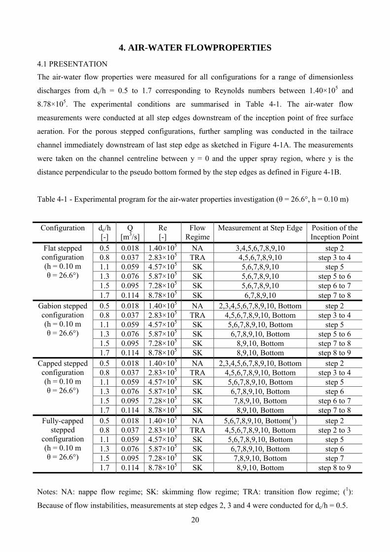
4. AIR-WATER FLOWPROPERTIES
4.1 PRESENTATION
The air-water flow properties were measured for all configurations for a range of dimensionless
discharges from dc/h = 0.5 to 1.7 corresponding to Reynolds numbers between 1.40×10⁵ and
8.78×10⁵. The experimental conditions are summarised in Table 4-1. The air-water flow
measurements were conducted at all step edges downstream of the inception point of free surface
aeration. For the porous stepped configurations, further sampling was conducted in the tailrace
channel immediately downstream of last step edge as sketched in Figure 4-1A. The measurements
were taken on the channel centreline between y = 0 and the upper spray region, where y is the
distance perpendicular to the pseudo bottom formed by the step edges as defined in Figure 4-1B.
Table 4-1 - Experimental program for the air-water properties investigation (θ = 26.6°, h = 0.10 m)
Configuration dc/h [-]
Q [m3/s]
Re [-]
Flow Regime
Measurement at Step Edge Position of the Inception Point
0.5 0.018 1.40×10⁵ NA 3,4,5,6,7,8,9,10 step 2 0.8 0.037 2.83×10⁵ TRA 4,5,6,7,8,9,10 step 3 to 4 1.1 0.059 4.57×10⁵ SK 5,6,7,8,9,10 step 5 1.3 0.076 5.87×10⁵ SK 5,6,7,8,9,10 step 5 to 6 1.5 0.095 7.28×10⁵ SK 5,6,7,8,9,10 step 6 to 7
Flat stepped configuration (h = 0.10 m θ = 26.6°)
1.7 0.114 8.78×10⁵ SK 6,7,8,9,10 step 7 to 8 0.5 0.018 1.40×10⁵ NA 2,3,4,5,6,7,8,9,10, Bottom step 2 0.8 0.037 2.83×10⁵ TRA 4,5,6,7,8,9,10, Bottom step 3 to 4 1.1 0.059 4.57×10⁵ SK 5,6,7,8,9,10, Bottom step 5 1.3 0.076 5.87×10⁵ SK 6,7,8,9,10, Bottom step 5 to 6 1.5 0.095 7.28×10⁵ SK 8,9,10, Bottom step 7 to 8
Gabion stepped configuration (h = 0.10 m θ = 26.6°)
1.7 0.114 8.78×10⁵ SK 8,9,10, Bottom step 8 to 9 0.5 0.018 1.40×10⁵ NA 2,3,4,5,6,7,8,9,10, Bottom step 2 0.8 0.037 2.83×10⁵ TRA 4,5,6,7,8,9,10, Bottom step 3 to 4 1.1 0.059 4.57×10⁵ SK 5,6,7,8,9,10, Bottom step 5 1.3 0.076 5.87×10⁵ SK 6,7,8,9,10, Bottom step 6 1.5 0.095 7.28×10⁵ SK 7,8,9,10, Bottom step 6 to 7
Capped stepped configuration (h = 0.10 m θ = 26.6°)
1.7 0.114 8.78×10⁵ SK 8,9,10, Bottom step 7 to 8 0.5 0.018 1.40×10⁵ NA 5,6,7,8,9,10, Bottom(1) step 2 0.8 0.037 2.83×10⁵ TRA 4,5,6,7,8,9,10, Bottom step 2 to 3 1.1 0.059 4.57×10⁵ SK 5,6,7,8,9,10, Bottom step 5 1.3 0.076 5.87×10⁵ SK 6,7,8,9,10, Bottom step 6 1.5 0.095 7.28×10⁵ SK 7,8,9,10, Bottom step 7
Fully-capped stepped
configuration (h = 0.10 m θ = 26.6°)
1.7 0.114 8.78×10⁵ SK 8,9,10, Bottom step 8 to 9
Notes: NA: nappe flow regime; SK: skimming flow regime; TRA: transition flow regime; (1):
Because of flow instabilities, measurements at step edges 2, 3 and 4 were conducted for dc/h = 0.5.
21
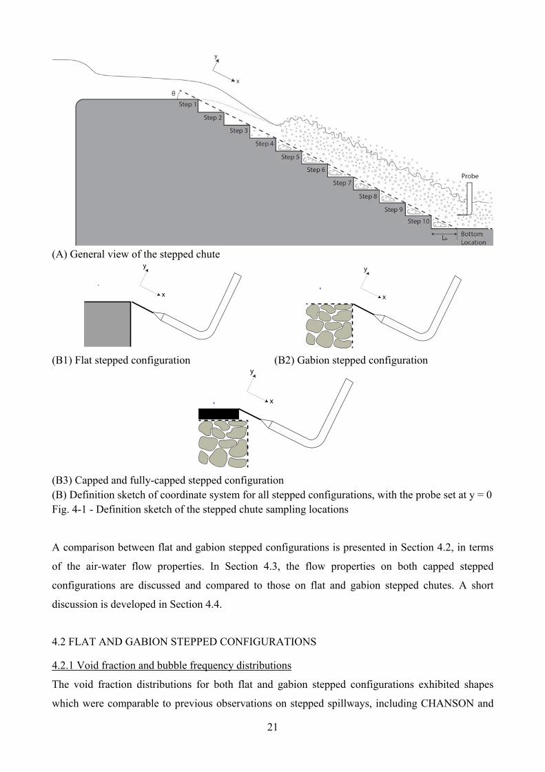
(A) General view of the stepped chute
(B1) Flat stepped configuration (B2) Gabion stepped configuration
(B3) Capped and fully-capped stepped configuration (B) Definition sketch of coordinate system for all stepped configurations, with the probe set at y = 0Fig. 4-1 - Definition sketch of the stepped chute sampling locations
A comparison between flat and gabion stepped configurations is presented in Section 4.2, in terms
of the air-water flow properties. In Section 4.3, the flow properties on both capped stepped
configurations are discussed and compared to those on flat and gabion stepped chutes. A short
discussion is developed in Section 4.4.
4.2 FLAT AND GABION STEPPED CONFIGURATIONS
4.2.1 Void fraction and bubble frequency distributions
The void fraction distributions for both flat and gabion stepped configurations exhibited shapes
which were comparable to previous observations on stepped spillways, including CHANSON and
22
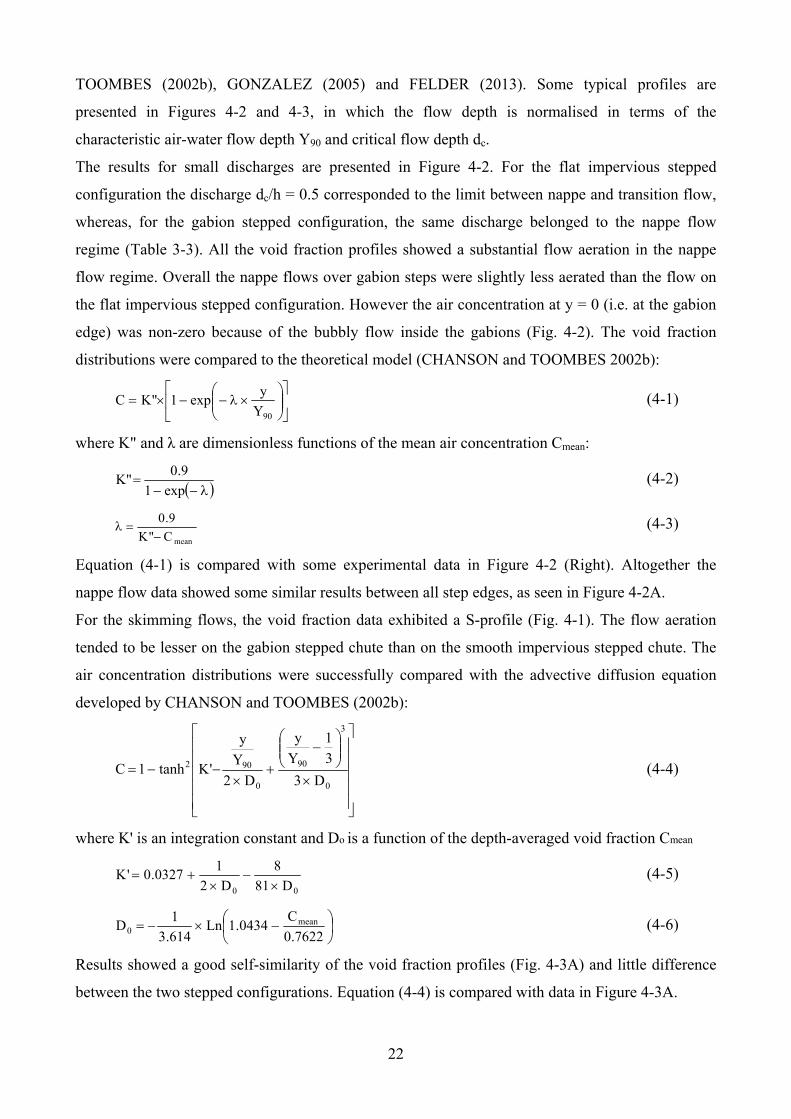
TOOMBES (2002b), GONZALEZ (2005) and FELDER (2013). Some typical profiles are
presented in Figures 4-2 and 4-3, in which the flow depth is normalised in terms of the
characteristic air-water flow depth Y90 and critical flow depth dc.
The results for small discharges are presented in Figure 4-2. For the flat impervious stepped
configuration the discharge dc/h = 0.5 corresponded to the limit between nappe and transition flow,
whereas, for the gabion stepped configuration, the same discharge belonged to the nappe flow
regime (Table 3-3). All the void fraction profiles showed a substantial flow aeration in the nappe
flow regime. Overall the nappe flows over gabion steps were slightly less aerated than the flow on
the flat impervious stepped configuration. However the air concentration at y = 0 (i.e. at the gabion
edge) was non-zero because of the bubbly flow inside the gabions (Fig. 4-2). The void fraction
distributions were compared to the theoretical model (CHANSON and TOOMBES 2002b):
90Y
yexp1"KC (4-1)
where K" and λ are dimensionless functions of the mean air concentration Cmean:
exp1
9.0"K (4-2)
meanC"K
9.0
(4-3)
Equation (4-1) is compared with some experimental data in Figure 4-2 (Right). Altogether the
nappe flow data showed some similar results between all step edges, as seen in Figure 4-2A.
For the skimming flows, the void fraction data exhibited a S-profile (Fig. 4-1). The flow aeration
tended to be lesser on the gabion stepped chute than on the smooth impervious stepped chute. The
air concentration distributions were successfully compared with the advective diffusion equation
developed by CHANSON and TOOMBES (2002b):
0
3
90
0
902
D3
3
1
Y
y
D2
Y
y
'Ktanh1C (4-4)
where K' is an integration constant and Do is a function of the depth-averaged void fraction Cmean
00 D81
8
D2
10327.0'K
(4-5)
7622.0
C0434.1Ln
614.3
1D mean
0 (4-6)
Results showed a good self-similarity of the void fraction profiles (Fig. 4-3A) and little difference
between the two stepped configurations. Equation (4-4) is compared with data in Figure 4-3A.
23
C
y/d c
0 0.1 0.2 0.3 0.4 0.5 0.6 0.7 0.8 0.9 10
0.25
0.5
0.75
1
1.25
1.5
1.75
2
2.25
2.5Flat Steps - Step edge 6Flat Steps - Step edge 7Flat Steps - Step edge 8Flat Steps - Step edge 9Flat Steps - Step edge 10Gabion Steps - Step edge 6Gabion Steps - Step edge 7Gabion Steps - Step edge 8Gabion Steps - Step edge 9Gabion Steps - Step edge 10
Cy/
Y90
0 0.1 0.2 0.3 0.4 0.5 0.6 0.7 0.8 0.9 10
0.2
0.4
0.6
0.8
1
1.2
1.4
1.6
1.8
2
2.2 Flat Steps - Step edge 6Flat Steps - Step edge 7Flat Steps - Step edge 8Flat Steps - Step edge 9Flat Steps - Step edge 10Gabion Steps - Step edge 6Gabion Steps - Step edge 7Gabion Steps - Step edge 8Gabion Steps - Step edge 9Gabion Steps - Step edge 10Theory step 10 - FlatTheory step 10 - Gabion
Fig. 4-2 - Comparison of void fraction distributions for flat and gabion stepped configurations,
nappe flow regime ( = 26.6°, h = 0.10 m) - dc/h = 0.5, Q = 0.018 m3/s, Re = 1.40×10⁵
C
y/Y
90
0 0.1 0.2 0.3 0.4 0.5 0.6 0.7 0.8 0.9 10
0.2
0.4
0.6
0.8
1
1.2
1.4
1.6
1.8 Flat steps - Step edge 7Flat steps - Step edge 8Flat steps - Step edge 9Flat steps - Step edge 10Gabion steps - Step edge 7Gabion steps - Step edge 8Gabion steps - Step edge 9Gabion steps - Step edge 10Theory step 10 - FlatTheory step 10 - Gabion
C
y/d c
0 0.1 0.2 0.3 0.4 0.5 0.6 0.7 0.8 0.9 10
0.2
0.4
0.6
0.8 Flat steps - Step edge 8Flat steps - Step edge 9Flat steps - Step edge 10Gabion steps - Step edge 8Gabion steps - Step edge 9Gabion steps - Step edge 10
(A) dc/h = 1.3, Q = 0.076 m3/s, Re = 5.9×10⁵ (B) dc/h = 1.5, Q = 0.095 m3/s, Re = 7.3×10⁵
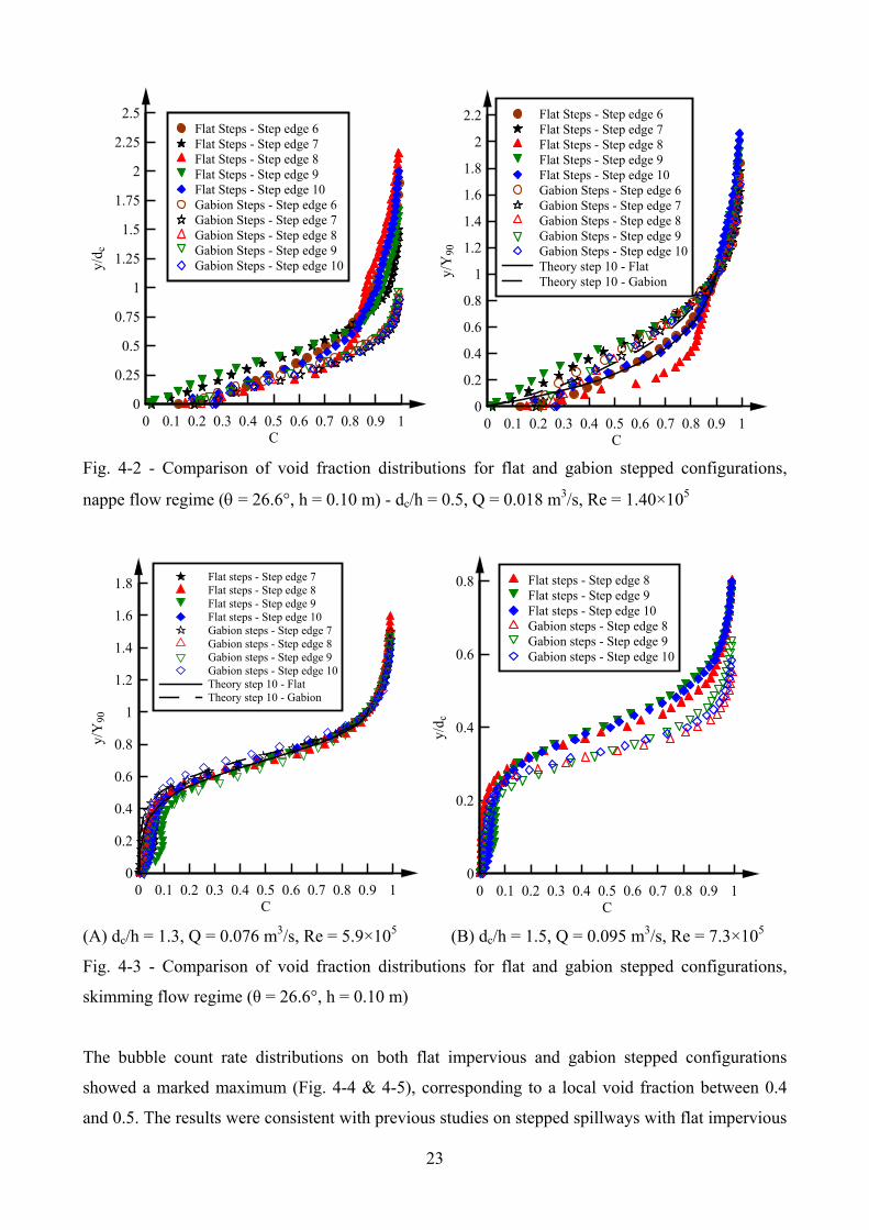
Fig. 4-3 - Comparison of void fraction distributions for flat and gabion stepped configurations,
skimming flow regime (θ = 26.6°, h = 0.10 m)
The bubble count rate distributions on both flat impervious and gabion stepped configurations
showed a marked maximum (Fig. 4-4 & 4-5), corresponding to a local void fraction between 0.4
and 0.5. The results were consistent with previous studies on stepped spillways with flat impervious
24
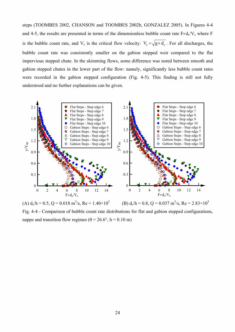
steps (TOOMBES 2002, CHANSON and TOOMBES 2002b, GONZALEZ 2005). In Figures 4-4
and 4-5, the results are presented in terms of the dimensionless bubble count rate Fdc/Vc where F
is the bubble count rate, and Vc is the critical flow velocity: cc dgV . For all discharges, the
bubble count rate was consistently smaller on the gabion stepped weir compared to the flat
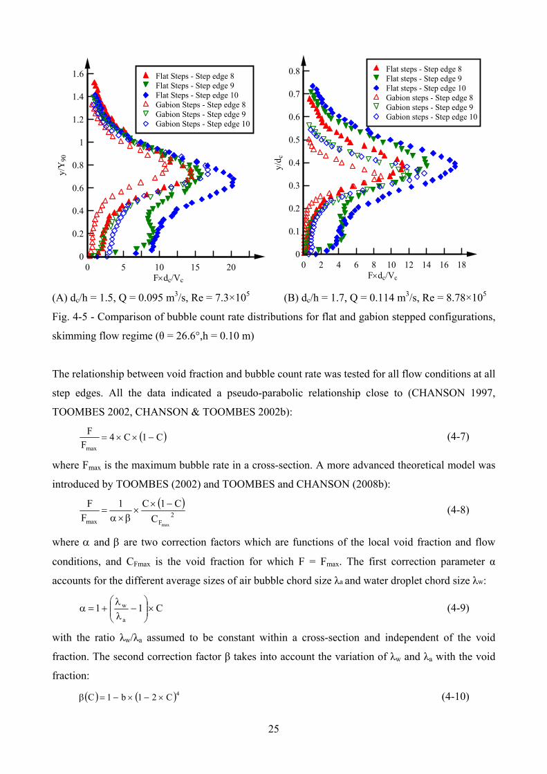
impervious stepped chute. In the skimming flows, some difference was noted between smooth and
gabion stepped chutes in the lower part of the flow: namely, significantly less bubble count rates
were recorded in the gabion stepped configuration (Fig. 4-5). This finding is still not fully
understood and no further explanations can be given.
Fdc/Vc
y/Y
90
0 2 4 6 8 10 12 140
0.3
0.6
0.9
1.2
1.5
1.8
2.1 Flat Steps - Step edge 6Flat Steps - Step edge 7Flat Steps - Step edge 8Flat Steps - Step edge 9Flat Steps - Step edge 10Gabion Steps - Step edge 6Gabion Steps - Step edge 7Gabion Steps - Step edge 8Gabion Steps - Step edge 9Gabion Steps - Step edge 10
(A) dc/h = 0.5, Q = 0.018 m3/s, Re = 1.40×10⁵ (B) dc/h = 0.8, Q = 0.037 m3/s, Re = 2.83×10⁵
Fig. 4-4 - Comparison of bubble count rate distributions for flat and gabion stepped configurations,
nappe and transition flow regimes (θ = 26.6°, h = 0.10 m)
25
Fdc/Vc
y/Y
90
0 5 10 15 200
0.2
0.4
0.6
0.8
1
1.2
1.4
1.6 Flat Steps - Step edge 8Flat Steps - Step edge 9Flat Steps - Step edge 10Gabion Steps - Step edge 8Gabion Steps - Step edge 9Gabion Steps - Step edge 10
Fdc/Vcy/
d c
0 2 4 6 8 10 12 14 16 180
0.1
0.2
0.3
0.4
0.5
0.6
0.7
0.8 Flat steps - Step edge 8Flat steps - Step edge 9Flat steps - Step edge 10Gabion steps - Step edge 8Gabion steps - Step edge 9Gabion steps - Step edge 10
(A) dc/h = 1.5, Q = 0.095 m3/s, Re = 7.3×10⁵ (B) dc/h = 1.7, Q = 0.114 m3/s, Re = 8.78×10⁵
Fig. 4-5 - Comparison of bubble count rate distributions for flat and gabion stepped configurations,
skimming flow regime (θ = 26.6°,h = 0.10 m)
The relationship between void fraction and bubble count rate was tested for all flow conditions at all
step edges. All the data indicated a pseudo-parabolic relationship close to (CHANSON 1997,
TOOMBES 2002, CHANSON & TOOMBES 2002b):
C1C4F
F
max
(4-7)
where Fmax is the maximum bubble rate in a cross-section. A more advanced theoretical model was
introduced by TOOMBES (2002) and TOOMBES and CHANSON (2008b):
2Fmax
maxC
C1C1
F
F
(4-8)
where and are two correction factors which are functions of the local void fraction and flow
conditions, and CFmax is the void fraction for which F = Fmax. The first correction parameter α
accounts for the different average sizes of air bubble chord size λa and water droplet chord size λw:
C11a
w
(4-9)
with the ratio λw/λa assumed to be constant within a cross-section and independent of the void
fraction. The second correction factor β takes into account the variation of λw and λa with the void
fraction:
4C21b1C (4-10)
26
where b is a characteristic value of the maximum variation of β: i.e., 1-b < β < 1 (TOOMBES and
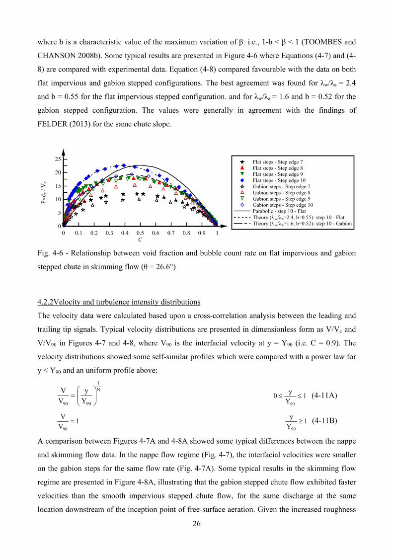
CHANSON 2008b). Some typical results are presented in Figure 4-6 where Equations (4-7) and (4-
8) are compared with experimental data. Equation (4-8) compared favourable with the data on both
flat impervious and gabion stepped configurations. The best agreement was found for λw/λa = 2.4
and b = 0.55 for the flat impervious stepped configuration. and for λw/λa = 1.6 and b = 0.52 for the
gabion stepped configuration. The values were generally in agreement with the findings of
FELDER (2013) for the same chute slope.
C
Fd
c / V
c
0 0.1 0.2 0.3 0.4 0.5 0.6 0.7 0.8 0.9 10
5
10
15
20
25 Flat steps - Step edge 7Flat steps - Step edge 8Flat steps - Step edge 9Flat steps - Step edge 10Gabion steps - Step edge 7Gabion steps - Step edge 8Gabion steps - Step edge 9Gabion steps - Step edge 10Parabolic - step 10 - FlatTheory (w/a=2.4, b=0.55)- step 10 - FlatTheory (w/a=1.6, b=0.52)- step 10 - Gabion
Fig. 4-6 - Relationship between void fraction and bubble count rate on flat impervious and gabion
stepped chute in skimming flow (θ = 26.6°)
4.2.2Velocity and turbulence intensity distributions
The velocity data were calculated based upon a cross-correlation analysis between the leading and
trailing tip signals. Typical velocity distributions are presented in dimensionless form as V/Vc and
V/V90 in Figures 4-7 and 4-8, where V90 is the interfacial velocity at y = Y90 (i.e. C = 0.9). The
velocity distributions showed some self-similar profiles which were compared with a power law for
y < Y90 and an uniform profile above:
N
1
9090 Y
y
V
V
1
Y
y0
90
(4-11A)
1V
V
90
1Y
y
90
(4-11B)
A comparison between Figures 4-7A and 4-8A showed some typical differences between the nappe
and skimming flow data. In the nappe flow regime (Fig. 4-7), the interfacial velocities were smaller
on the gabion steps for the same flow rate (Fig. 4-7A). Some typical results in the skimming flow
regime are presented in Figure 4-8A, illustrating that the gabion stepped chute flow exhibited faster
velocities than the smooth impervious stepped chute flow, for the same discharge at the same
location downstream of the inception point of free-surface aeration. Given the increased roughness
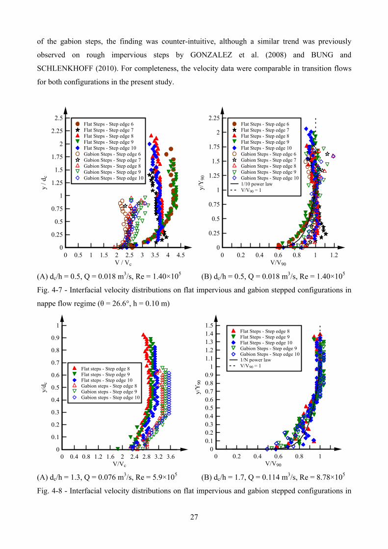
27
of the gabion steps, the finding was counter-intuitive, although a similar trend was previously
observed on rough impervious steps by GONZALEZ et al. (2008) and BUNG and
SCHLENKHOFF (2010). For completeness, the velocity data were comparable in transition flows
for both configurations in the present study.
V / Vc
y / d
c
0 0.5 1 1.5 2 2.5 3 3.5 4 4.50
0.25
0.5
0.75
1
1.25
1.5
1.75
2
2.25
2.5Flat Steps - Step edge 6Flat Steps - Step edge 7Flat Steps - Step edge 8Flat Steps - Step edge 9Flat Steps - Step edge 10Gabion Steps - Step edge 6Gabion Steps - Step edge 7Gabion Steps - Step edge 8Gabion Steps - Step edge 9Gabion Steps - Step edge 10
V/V90
y/Y
90
0 0.2 0.4 0.6 0.8 1 1.20
0.25
0.5
0.75
1
1.25
1.5
1.75
2
2.25Flat Steps - Step edge 6Flat Steps - Step edge 7Flat Steps - Step edge 8Flat Steps - Step edge 9Flat Steps - Step edge 10Gabion Steps - Step edge 6Gabion Steps - Step edge 7Gabion Steps - Step edge 8Gabion Steps - Step edge 9Gabion Steps - Step edge 101/10 power lawV/V90 = 1
(A) dc/h = 0.5, Q = 0.018 m3/s, Re = 1.40×10⁵ (B) dc/h = 0.5, Q = 0.018 m3/s, Re = 1.40×10⁵
Fig. 4-7 - Interfacial velocity distributions on flat impervious and gabion stepped configurations in
nappe flow regime (θ = 26.6°, h = 0.10 m)
V/Vc
y/d c
0 0.4 0.8 1.2 1.6 2 2.4 2.8 3.2 3.60
0.1
0.2
0.3
0.4
0.5
0.6
0.7
0.8
0.9
1
Flat steps - Step edge 8Flat steps - Step edge 9Flat steps - Step edge 10Gabion steps - Step edge 8Gabion steps - Step edge 9Gabion steps - Step edge 10
V/V90
y/Y
90
0 0.2 0.4 0.6 0.8 10
0.10.20.30.40.50.60.70.80.9
11.11.21.31.41.5
Flat Steps - Step edge 8Flat Steps - Step edge 9Flat Steps - Step edge 10Gabion Steps - Step edge 9Gabion Steps - Step edge 101/N power lawV/V90 = 1
(A) dc/h = 1.3, Q = 0.076 m3/s, Re = 5.9×10⁵ (B) dc/h = 1.7, Q = 0.114 m3/s, Re = 8.78×10⁵
Fig. 4-8 - Interfacial velocity distributions on flat impervious and gabion stepped configurations in

28
skimming flow regime (θ = 26.6°, h = 0.10 m)
Tu
y/d c
0 0.5 1 1.5 2 2.50
0.25
0.5
0.75
1
1.25
1.5
1.75
2
2.25
2.5 Flat Steps - Step edge 6Flat Steps - Step edge 7Flat Steps - Step edge 8Flat Steps - Step edge 9Flat Steps - Step edge 10Gabion Steps - Step edge 6Gabion Steps - Step edge 7Gabion Steps - Step edge 8Gabion Steps - Step edge 9Gabion Steps - Step edge 10
Tu
y/Y
90
0 0.4 0.8 1.2 1.6 2 2.4 2.80
0.2
0.4
0.6
0.8
1
1.2
1.4
1.6
1.8
2
2.2
2.4Flat Steps - Step edge 7Flat Steps - Step edge 8Flat Steps - Step edge 9Flat Steps - Step edge 10Gabion Steps - Step edge 7Gabion Steps - Step edge 8Gabion Steps - Step edge 9Gabion Steps - Step edge 10
(A) dc/h = 0.5, Q = 0.018 m3/s, Re = 1.40×10⁵ (B) dc/h = 0.8, Q = 0.037 m3/s, Re = 2.83×10⁵
Fig. 4-9 - Turbulence intensity distributions on flat impervious and gabion stepped configuration in
nappe and transition flow regimes (θ = 26.6°, h = 0.10 m)
Tu
y/Y
90
0 0.5 1 1.5 2 2.50
0.2
0.4
0.6
0.8
1
1.2
1.4
1.6
1.8Flat Steps - Step edge 8Flat Steps - Step edge 9Flat Steps - Step edge 10Gabion Steps - Step edge 8Gabion Steps - Step edge 9Gabion Steps - Step edge 10
Tu
y/d c
0 0.4 0.8 1.2 1.6 2 2.4 2.80
0.1
0.2
0.3
0.4
0.5
0.6
0.7
0.8 Flat steps - Step edge 8Flat steps - Step edge 9Flat steps - Step edge 10Gabion steps - Step edge 8Gabion steps - Step edge 9Gabion steps - Step edge 10
(A) dc/h = 1.1, Q = 0.059 m3/s, Re = 4.57×10⁵ (B) dc/h = 1.5, Q = 0.095 m3/s, Re = 7.3×10⁵
Fig. 4-10 - Turbulence intensity distributions on flat and gabion stepped configurations in skimming
flow regime (θ = 26.6°, h = 0.10 m)
Equation (4-11) is compared with some experimental data in Figure 4-7B and 4-8B, using a power
29
law exponent of 1/N = 1/10.
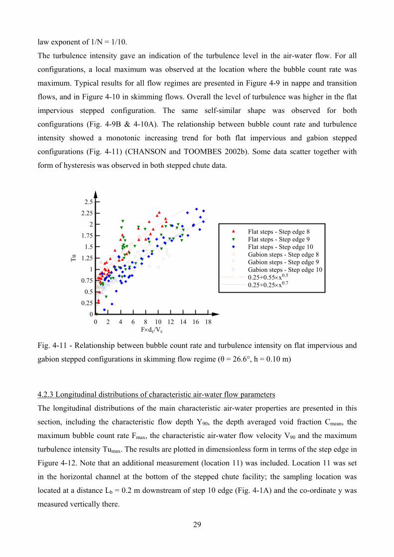
The turbulence intensity gave an indication of the turbulence level in the air-water flow. For all
configurations, a local maximum was observed at the location where the bubble count rate was
maximum. Typical results for all flow regimes are presented in Figure 4-9 in nappe and transition
flows, and in Figure 4-10 in skimming flows. Overall the level of turbulence was higher in the flat
impervious stepped configuration. The same self-similar shape was observed for both
configurations (Fig. 4-9B & 4-10A). The relationship between bubble count rate and turbulence
intensity showed a monotonic increasing trend for both flat impervious and gabion stepped
configurations (Fig. 4-11) (CHANSON and TOOMBES 2002b). Some data scatter together with
form of hysteresis was observed in both stepped chute data.
Fdc/Vc
Tu
0 2 4 6 8 10 12 14 16 180
0.25
0.5
0.75
1
1.25
1.5
1.75
2
2.25
2.5
Flat steps - Step edge 8Flat steps - Step edge 9Flat steps - Step edge 10Gabion steps - Step edge 8Gabion steps - Step edge 9Gabion steps - Step edge 100.25+0.55x0.5
0.25+0.25x0.7
Fig. 4-11 - Relationship between bubble count rate and turbulence intensity on flat impervious and
gabion stepped configurations in skimming flow regime (θ = 26.6°, h = 0.10 m)
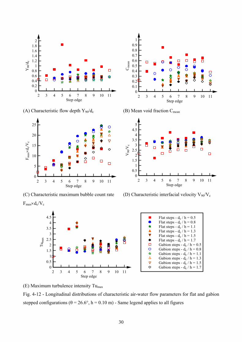
4.2.3 Longitudinal distributions of characteristic air-water flow parameters
The longitudinal distributions of the main characteristic air-water properties are presented in this
section, including the characteristic flow depth Y90, the depth averaged void fraction Cmean, the
maximum bubble count rate Fmax, the characteristic air-water flow velocity V90 and the maximum
turbulence intensity Tumax. The results are plotted in dimensionless form in terms of the step edge in
Figure 4-12. Note that an additional measurement (location 11) was included. Location 11 was set
in the horizontal channel at the bottom of the stepped chute facility; the sampling location was
located at a distance Lb = 0.2 m downstream of step 10 edge (Fig. 4-1A) and the co-ordinate y was
measured vertically there.
30
Step edge
Y90
/dc
2 3 4 5 6 7 8 9 10 110
0.20.40.60.8
11.21.41.61.8
2
Step edge
Cm
ean
2 3 4 5 6 7 8 9 10 110
0.10.20.30.40.50.60.70.80.9
1
(A) Characteristic flow depth Y90/dc (B) Mean void fraction Cmean
Step edge
Fm
axd
c/V
c
2 3 4 5 6 7 8 9 10 110
5
10
15
20
25
Step edge
V90
/Vc
2 3 4 5 6 7 8 9 10 110
0.51
1.52
2.53
3.54
4.55
(C) Characteristic maximum bubble count rate
Fmaxdc/Vc
(D) Characteristic interfacial velocity V90/Vc
Step edge
Tu m
ax
2 3 4 5 6 7 8 9 10 110
0.5
1
1.5
2
2.5
3
3.5
4
4.5 Flat steps - dc / h = 0.5Flat steps - dc / h = 0.8Flat steps - dc / h = 1.1Flat steps - dc / h = 1.3Flat steps - dc / h = 1.5Flat steps - dc / h = 1.7Gabion steps - dc / h = 0.5Gabion steps - dc / h = 0.8Gabion steps - dc / h = 1.1Gabion steps - dc / h = 1.3Gabion steps - dc / h = 1.5Gabion steps - dc / h = 1.7
(E) Maximum turbulence intensity Tumax
Fig. 4-12 - Longitudinal distributions of characteristic air-water flow parameters for flat and gabion
stepped configurations (θ = 26.6°, h = 0.10 m) - Same legend applies to all figures
31
Figure 4-12A presents the dimensionless characteristic flow depth Y90/dc. The results showed that
the air-water flow height was lower for all discharges on the gabion stepped configuration. The
largest differences between the two stepped configurations were seen with the nappe flow regime,
for which the gabion stepped chute flow presented an almost evenly distributed flow heights. The
depth-averaged void fraction data Cmean are presented in Figure 4-12B. The results highlighted a
lesser aeration of the flow on the gabion stepped configuration. At the step edge 10, the depth-
averaged void fraction was between 1.0 and 1.4 times larger on the flat impervious stepped chute
than on the gabion stepped chute, and the difference increased monotonically with an increasing
discharge (Fig. 4-12B). The maximum bubble count rate Fmax×dc/Vc increased monotonically with
the downstream direction for all discharges and all configurations. Smaller maximum bubble counts
were recorded on the gabion stepped chute for both nappe and skimming flows (Fig. 4-12C).
Figure 4-12D shows the characteristic air-water velocity V90/Vc as function of the longitudinal
distance. Although the step surface roughness was larger on the gabion steps, the data showed that,
in the skimming flow regime, the velocities on gabion steps were larger than those on the flat
smooth stepped configuration (Fig. 4-12D). Although counter-intuitive, these results were similar to
the findings of GONZALEZ et al. (2008) for rough impervious steps. On the other hand, for the
nappe flow regime, the air-water velocities were smaller on the gabion steps. The longitudinal
distributions of maximum turbulence intensity Tumax are presented in Figure 4-12E. At the
downstream end of the facility (step edge 10), Tumax ranged from 1.6 to 2.5 for all configurations.
However, for all discharges, the maximum turbulence intensity observed over the smooth
impervious stepped structure was on average 12% larger than that recorded on the gabion stepped
chute.
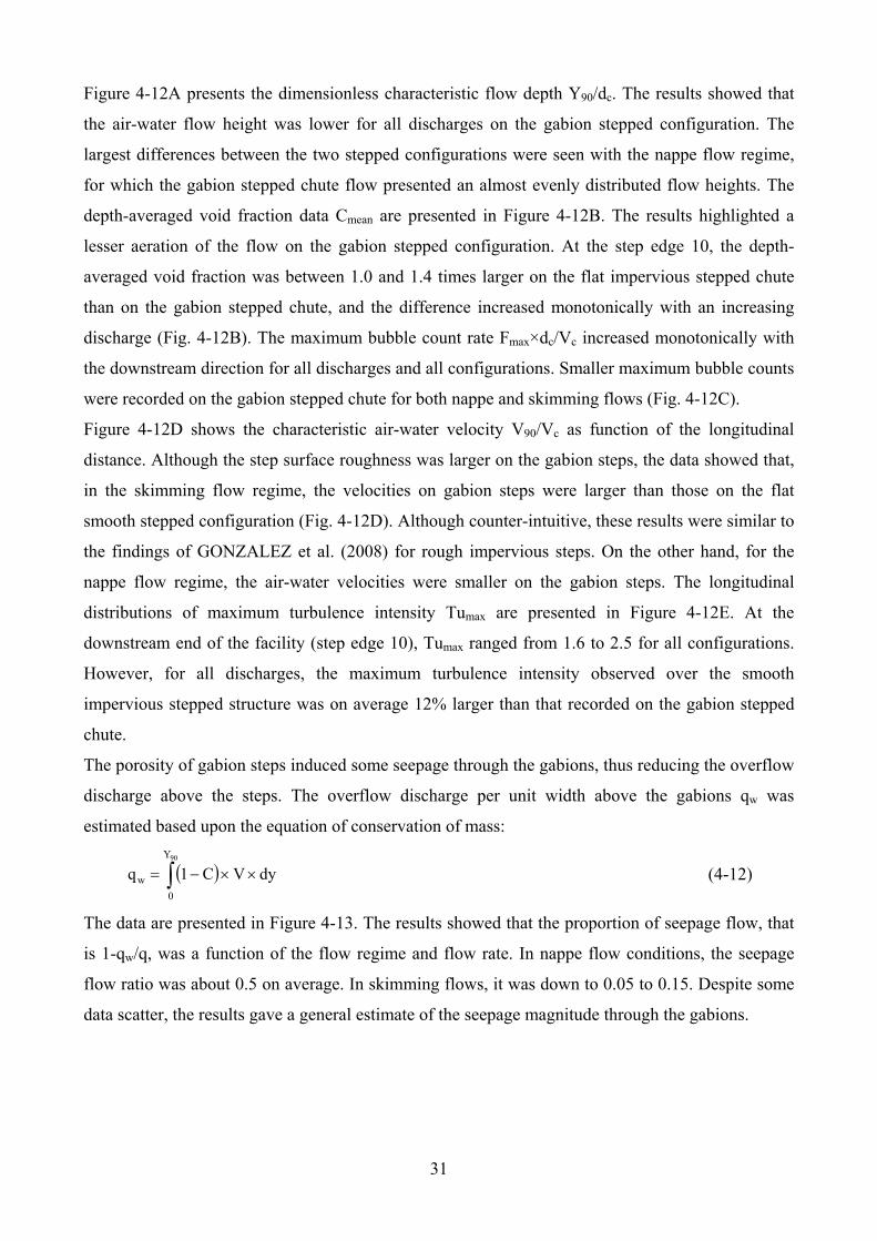
The porosity of gabion steps induced some seepage through the gabions, thus reducing the overflow
discharge above the steps. The overflow discharge per unit width above the gabions qw was
estimated based upon the equation of conservation of mass:
90Y
0
w dyVC1q (4-12)
The data are presented in Figure 4-13. The results showed that the proportion of seepage flow, that
is 1-qw/q, was a function of the flow regime and flow rate. In nappe flow conditions, the seepage
flow ratio was about 0.5 on average. In skimming flows, it was down to 0.05 to 0.15. Despite some
data scatter, the results gave a general estimate of the seepage magnitude through the gabions.
32
Step edge
q w/q
0 1 2 3 4 5 6 7 8 9 10 110
0.20.40.60.8
11.21.41.61.8
2
Flat steps - dc / h = 0.5Flat steps - dc / h = 0.8Flat steps - dc / h = 1.1Flat steps - dc / h = 1.3Flat steps - dc / h = 1.5Flat steps - dc / h = 1.7
Gabion steps - dc / h = 0.5Gabion steps - dc / h = 0.8Gabion steps - dc / h = 1.1Gabion steps - dc / h = 1.3Gabion steps - dc / h = 1.5Gabion steps - dc / h = 1.7
Fig. 4-13-Discharge ratio qw/q between the measured volume flux and the total discharge per unit
width
4.3 CAPPED AND FULLY-CAPPED STEPPED CONFIGURATIONS
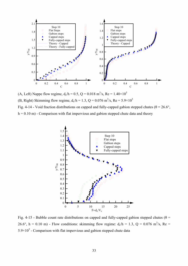
4.3.1 Void fraction and bubble frequency distributions
For both capped gabion configurations, detailed air-water flow measurements were conducted.
Some typical void fraction profiles are presented in Figure 4-14. The data exhibited similar trends to
those obtained for both gabion and flat stepped configurations, as well as earlier stepped chute
studies with comparable slopes (CHANSON and TOOMBES 2002b, GONZALEZ 2005, FELDER
2013). Figure 4-14A shows some data for low discharges corresponding to a nappe flow regime.
Figure 4-14B presents some skimming flow data. Overall the behaviour of both capped and fully
capped gabion stepped configurations was in between the gabion and the flat stepped
configurations; the fully capped stepped configuration presenting results very similar to those on the
flat impervious stepped chute.
In terms of bubble count rate distributions, all stepped configurations presented a similar data shape
with a marked maximum corresponding at C 0.4-0.5 (Fig. 4-15). The capped and fully-capped
data yielded quantitative results which were generally similar to the flat stepped configuration data.
33
C
y/Y
90
0 0.2 0.4 0.6 0.8 10
0.3
0.6
0.9
1.2
1.5
1.8
2.1Step 10
Flat StepsGabion stepsCapped stepsFully-capped stepsTheory - CappedTheory - Fully-capped
C
y/Y
90
0 0.2 0.4 0.6 0.8 10
0.2
0.4
0.6
0.8
1
1.2
1.4
1.6Step 10
Flat stepsGabion stepsCapped stepsFully-capped stepsTheory - Capped
(A, Left) Nappe flow regime, dc/h = 0.5, Q = 0.018 m3/s, Re = 1.40×10⁵
(B, Right) Skimming flow regime, dc/h = 1.3, Q = 0.076 m3/s, Re = 5.9×10⁵
Fig. 4-14 - Void fraction distributions on capped and fully-capped gabion stepped chutes (θ = 26.6°,
h = 0.10 m) - Comparison with flat impervious and gabion stepped chute data and theory
Fdc/Vc
y/Y
90
0 5 10 15 20 250
0.1
0.2
0.3
0.4
0.5
0.6
0.7
0.8
0.9
1
1.1
1.2
1.3
1.4
1.5
Step 10Flat stepsGabion stepsCapped stepsFully-capped steps
Fig. 4-15 - Bubble count rate distributions on capped and fully-capped gabion stepped chutes (θ =
26.6°, h = 0.10 m) - Flow conditions: skimming flow regime: dc/h = 1.3, Q = 0.076 m3/s, Re =
5.9×10⁵ - Comparison with flat impervious and gabion stepped chute data
34
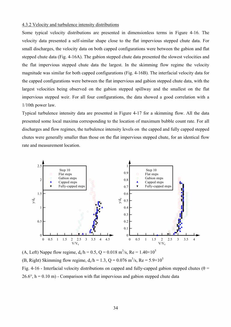
4.3.2 Velocity and turbulence intensity distributions
Some typical velocity distributions are presented in dimensionless terms in Figure 4-16. The
velocity data presented a self-similar shape close to the flat impervious stepped chute data. For
small discharges, the velocity data on both capped configurations were between the gabion and flat
stepped chute data (Fig. 4-16A). The gabion stepped chute data presented the slowest velocities and
the flat impervious stepped chute data the largest. In the skimming flow regime the velocity
magnitude was similar for both capped configurations (Fig. 4-16B). The interfacial velocity data for
the capped configurations were between the flat impervious and gabion stepped chute data, with the
largest velocities being observed on the gabion stepped spillway and the smallest on the flat
impervious stepped weir. For all four configurations, the data showed a good correlation with a
1/10th power law.
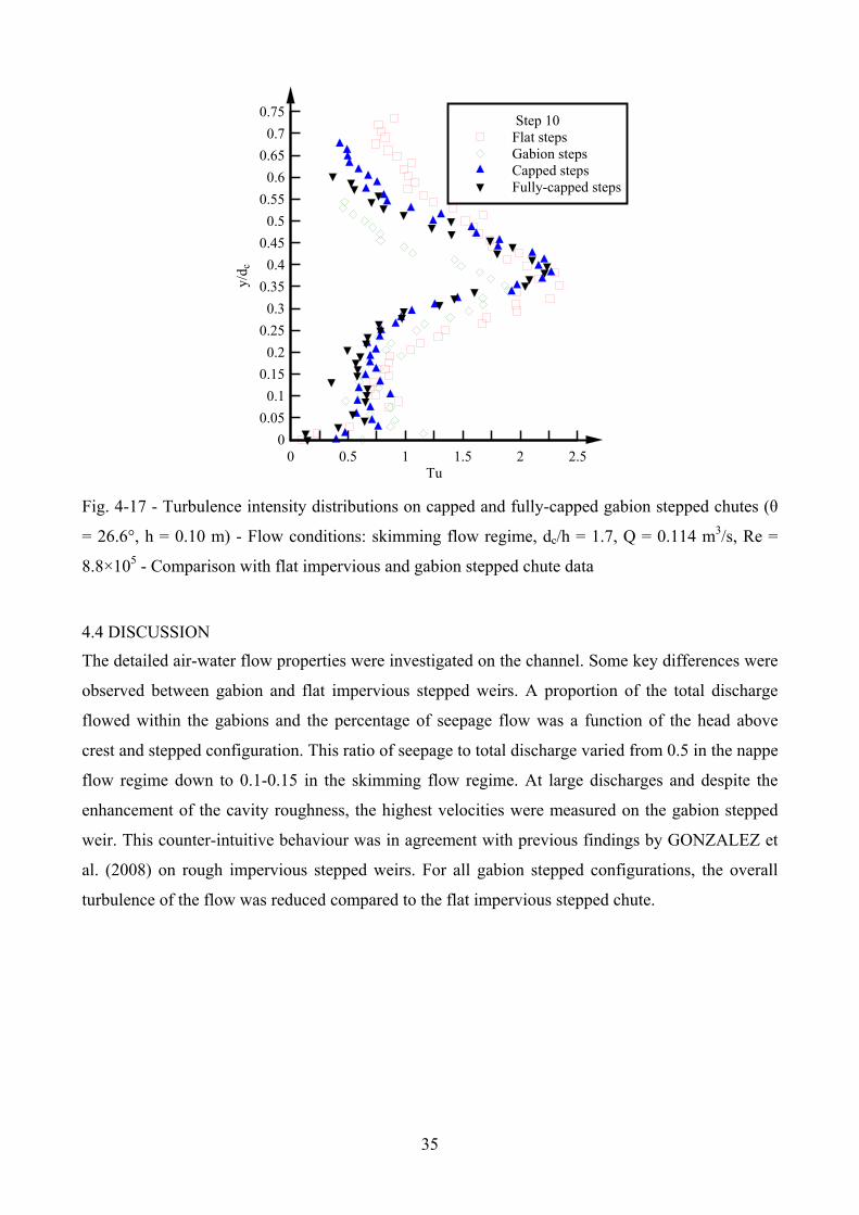
Typical turbulence intensity data are presented in Figure 4-17 for a skimming flow. All the data
presented some local maxima corresponding to the location of maximum bubble count rate. For all
discharges and flow regimes, the turbulence intensity levels on the capped and fully capped stepped
chutes were generally smaller than those on the flat impervious stepped chute, for an identical flow
rate and measurement location.
V/Vc
y/d c
0 0.5 1 1.5 2 2.5 3 3.5 4 4.50
0.5
1
1.5
2
2.5Step 10
Flat stepsGabion stepsCapped stepsFully-capped steps
V/Vc
y/d c
0 0.5 1 1.5 2 2.5 3 3.5 40
0.1
0.2
0.3
0.4
0.5
0.6
0.7
0.8
0.9
1Step 10
Flat stepsGabion stepsCapped stepsFully-capped steps
(A, Left) Nappe flow regime, dc/h = 0.5, Q = 0.018 m3/s, Re = 1.40×10⁵
(B, Right) Skimming flow regime, dc/h = 1.3, Q = 0.076 m3/s, Re = 5.9×10⁵
Fig. 4-16 - Interfacial velocity distributions on capped and fully-capped gabion stepped chutes (θ =
26.6°, h = 0.10 m) - Comparison with flat impervious and gabion stepped chute data
35
Tu
y/d c
0 0.5 1 1.5 2 2.50
0.05
0.1
0.15
0.2
0.25
0.3
0.35
0.4
0.45
0.5
0.55
0.6
0.65
0.7
0.75Step 10
Flat stepsGabion stepsCapped stepsFully-capped steps
Fig. 4-17 - Turbulence intensity distributions on capped and fully-capped gabion stepped chutes (θ
= 26.6°, h = 0.10 m) - Flow conditions: skimming flow regime, dc/h = 1.7, Q = 0.114 m3/s, Re =
8.8×10⁵ - Comparison with flat impervious and gabion stepped chute data
4.4 DISCUSSION
The detailed air-water flow properties were investigated on the channel. Some key differences were
observed between gabion and flat impervious stepped weirs. A proportion of the total discharge
flowed within the gabions and the percentage of seepage flow was a function of the head above
crest and stepped configuration. This ratio of seepage to total discharge varied from 0.5 in the nappe
flow regime down to 0.1-0.15 in the skimming flow regime. At large discharges and despite the
enhancement of the cavity roughness, the highest velocities were measured on the gabion stepped
weir. This counter-intuitive behaviour was in agreement with previous findings by GONZALEZ et
al. (2008) on rough impervious stepped weirs. For all gabion stepped configurations, the overall
turbulence of the flow was reduced compared to the flat impervious stepped chute.
36
5. ENERGY DISSIPATION AND FLOW RESISTANCE
5.1 RESIDUAL HEAD AND ENERGY DISSIPATION
For design purposes, the residual energy at the downstream end of the spillway chute is a key
parameter. The residual head was estimated from the air-water flow properties:
2Y
0
2Y
0
res90
90
dyC1g2
qcosdyC1H
(5-1A)
where C is the void fraction, y is the distance normal to the pseudo-bottom formed by the step
edges, Y90 is the characteristic height where C = 0.90, q is the water discharge per unit width, and g
is the gravity acceleration. Introducing the equivalent clear-water depth d and mean flow velocity
Uw = q/d, the residual head may be rewritten:
g2
UcosdH w
res (5-1B)
The energy loss was calculated as:
resmax HHH (5-2)
where Hmax is the upstream head above the sampling location. The rate of energy dissipation
∆H/Hmax expressed the percentage of total head loss above the stepped chute.
The results are presented in Figure 5-1 in terms of rate of energy dissipation at the downstream end
of the chute. Figure 5-1A shows the data at step edge 10 and Figure 5-1B the data in the
downstream tailrace channel. The data are presented as functions of the dimensionless drop in
elevation zo/dc between the broad crested weir and the sampling location. Note that the gabion
stepped data at step edge 10 were calculated using the overflow discharge estimate qw.
The experimental results showed that the gabion stepped weir was the least efficient in terms of
energy dissipation but for the smallest discharge. The three other stepped configurations (flat,
capped and fully-capped) yielded comparable results. For the smallest discharges (dc/h = 0.5), the
energy dissipation of the gabion stepped configuration was slightly larger than that on the flat
impervious stepped configuration. Between the step edge 10 and the tailrace channel, some
differences in terms of energy dissipation were seen for the gabion stepped chute which reflected
likely the large energy dissipation rate of the seepage flow component (STEPHENSON 1979).

37
z0/dc
H/H
max
0 2 4 6 8 10 12 14 16 18 200
0.1
0.2
0.3
0.4
0.5
0.6
0.7
0.8
0.9
1
Flat steps - Step edge 10Gabion steps - Step edge 10Capped steps - Step edge 10Fully-capped steps - Step edge 10
z0/dc
H/H
max
0 2 4 6 8 10 12 14 16 18 200
0.1
0.2
0.3
0.4
0.5
0.6
0.7
0.8
0.9
1
Gabion steps - BottomCapped steps - BottomFully-capped steps - Bottom
(A) Step edge 10 (B) Bottom (tailrace) channel
Fig. 5-1 - Rate of energy dissipation rate at the downstream end of flat impervious and gabion
stepped chutes (θ = 26.6°, h = 0.10 m)
dc/h
Hre
s/d c
0 0.2 0.4 0.6 0.8 1 1.2 1.4 1.6 1.80
0.5
1
1.5
2
2.5
3
3.5
4
4.5
5
5.5
6
6.5
7
Flat steps - Step 10Gabion steps - Step 10Capped steps - Step 10Fully-capped steps - Step 10
dc/h
Hre
s/d c
0 0.2 0.4 0.6 0.8 1 1.2 1.4 1.6 1.80
0.5
1
1.5
2
2.5
3
3.5
4
4.5
5
5.5
6
6.5
7
Gabion steps - BottomCapped steps - BottomFully-capped steps - Bottom
(A) Step edge 10 (B) Bottom (tailrace) channel
Fig. 5-2 - Residual head at the downstream end of flat impervious and gabion stepped chutes (θ =
26.6°, h = 0.10 m)
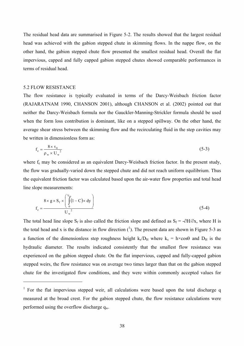
38
The residual head data are summarised in Figure 5-2. The results showed that the largest residual
head was achieved with the gabion stepped chute in skimming flows. In the nappe flow, on the
other hand, the gabion stepped chute flow presented the smallest residual head. Overall the flat
impervious, capped and fully capped gabion stepped chutes showed comparable performances in
terms of residual head.
5.2 FLOW RESISTANCE
The flow resistance is typically evaluated in terms of the Darcy-Weisbach friction factor
(RAJARATNAM 1990, CHANSON 2001), although CHANSON et al. (2002) pointed out that
neither the Darcy-Weisbach formula nor the Gauckler-Manning-Strickler formula should be used
when the form loss contribution is dominant, like on a stepped spillway. On the other hand, the
average shear stress between the skimming flow and the recirculating fluid in the step cavities may
be written in dimensionless form as:
2
ww
0e
U
8f
(5-3)
where fe may be considered as an equivalent Darcy-Weisbach friction factor. In the present study,
the flow was gradually-varied down the stepped chute and did not reach uniform equilibrium. Thus
the equivalent friction factor was calculated based upon the air-water flow properties and total head
line slope measurements:
2w
Y
0
f
eU
dyC1Sg8
f
90
(5-4)
The total head line slope Sf is also called the friction slope and defined as Sf = -∂H/∂x, where H is
the total head and x is the distance in flow direction (1). The present data are shown in Figure 5-3 as
a function of the dimensionless step roughness height ks/DH where ks = h×cos and DH is the
hydraulic diameter. The results indicated consistently that the smallest flow resistance was
experienced on the gabion stepped chute. On the flat impervious, capped and fully-capped gabion
stepped weirs, the flow resistance was on average two times larger than that on the gabion stepped
chute for the investigated flow conditions, and they were within commonly accepted values for
1 For the flat impervious stepped weir, all calculations were based upon the total discharge q
measured at the broad crest. For the gabion stepped chute, the flow resistance calculations were
performed using the overflow discharge qw.
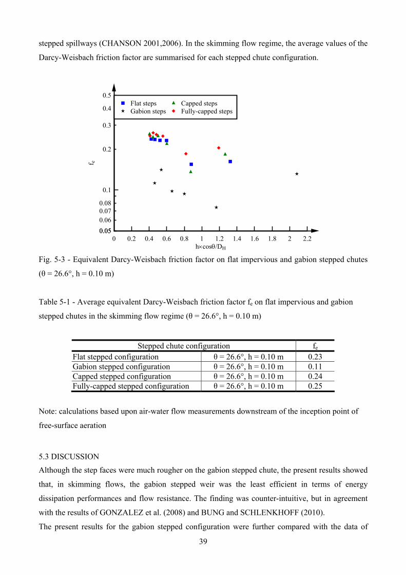
39
stepped spillways (CHANSON 2001,2006). In the skimming flow regime, the average values of the
Darcy-Weisbach friction factor are summarised for each stepped chute configuration.
hcos/DH
f e
0 0.2 0.4 0.6 0.8 1 1.2 1.4 1.6 1.8 2 2.20.050.05
0.060.070.08
0.1
0.2
0.3
0.4
0.5Flat stepsGabion steps
Capped stepsFully-capped steps
Fig. 5-3 - Equivalent Darcy-Weisbach friction factor on flat impervious and gabion stepped chutes
(θ = 26.6°, h = 0.10 m)
Table 5-1 - Average equivalent Darcy-Weisbach friction factor fe on flat impervious and gabion
stepped chutes in the skimming flow regime (θ = 26.6°, h = 0.10 m)
Stepped chute configuration fe Flat stepped configuration θ = 26.6°, h = 0.10 m 0.23 Gabion stepped configuration θ = 26.6°, h = 0.10 m 0.11 Capped stepped configuration θ = 26.6°, h = 0.10 m 0.24 Fully-capped stepped configuration θ = 26.6°, h = 0.10 m 0.25
Note: calculations based upon air-water flow measurements downstream of the inception point of
free-surface aeration
5.3 DISCUSSION
Although the step faces were much rougher on the gabion stepped chute, the present results showed
that, in skimming flows, the gabion stepped weir was the least efficient in terms of energy
dissipation performances and flow resistance. The finding was counter-intuitive, but in agreement
with the results of GONZALEZ et al. (2008) and BUNG and SCHLENKHOFF (2010).
The present results for the gabion stepped configuration were further compared with the data of
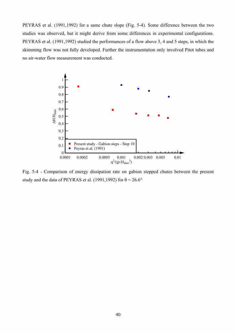
40
PEYRAS et al. (1991,1992) for a same chute slope (Fig. 5-4). Some difference between the two
studies was observed, but it might derive from some differences in experimental configurations.
PEYRAS et al. (1991,1992) studied the performances of a flow above 3, 4 and 5 steps, in which the
skimming flow was not fully developed. Further the instrumentation only involved Pitot tubes and
no air-water flow measurement was conducted.
q2/(gHdam3)
H/H
dam
0.0001 0.0002 0.0005 0.001 0.002 0.003 0.005 0.010
0.1
0.2
0.3
0.4
0.5
0.6
0.7
0.8
0.9
1
Present study - Gabion steps - Step 10Peyras et al. (1991)
Fig. 5-4 - Comparison of energy dissipation rate on gabion stepped chutes between the present
study and the data of PEYRAS et al. (1991,1992) for θ = 26.6°

41
6. INTERFACIAL AREA AND MASS TRANSFER RATE
6.1 PRESENTATION
Aeration in stepped spillways is a key feature linked with the strong flow turbulence, free-
surface/turbulent interactions and air entrainment (NAKASONE 1987, TOOMBES and CHANSON
2005). For the treatment of drinking water, cascade aeration can be used to reduce the chlorine
content, offensive taste and odours (CORSI et al. 1992). Re-oxygenation cascades were also built
downstream of dam spillways, and along rivers and canals (GASPAROTTO 1992, HAUSER et al.
1992, GOSSE and GREGOIRE 1997). The physical process of mass transfer is described by the
Fick’s law stating that the mass transfer rate across an interface varies proportionally to a diffusion
coefficient times the gradient of gas concentration:
x
CAD
t
M gasgas
gas (6-1)
where Mgas is the mass of dissolved gas, t is the time, Dgas is the diffusion coefficient of the gas in
the liquid, A is the gas-liquid interfacial area, Cgas is the concentration of the dissolved gas and x is
the direction in which the diffusion occurs. The equation for gas transfer across an air-water
interface can be rearranged as
gasSATLgas CCaKt
C
(6-2)
where KL is the mass transfer coefficient or liquid film coefficient, a is the specific interface area
defined as the interface area per unit volume, and CSAT is the amount of gas dissolved in water at
equilibrium (GULLIVER 1990). The rate of mass transfer is directly proportional to the specific
air-water interface area of the flow and therefore enhanced in highly aerated, turbulent flows
(TOOMBES and CHANSON 2005).
The specific interface area represents the cumulative surface of air bubbles that is encountered per
unit volume. In a turbulent air-water flow, it may be estimated as (CHANSON 2002):
V
F4a
(6-3)
where F is the bubble count rate and V is the interfacial velocity. In the present study, the specific
interface area profiles were estimated for all four stepped chute configurations for a wide range of
discharges (0.05 < Q < 0.114 m3/s) at all step edges downstream of the inception point of free-
surface aeration. The depth-averaged specific interface area amean was calculated as
90Y
090mean dya
Y
1a (6-4)
Some typical vertical distributions of specific interface area are shown in Figure 6-1A. The data

42
showed systematically a marked maximum corresponding to the location of maximum bubble count
rate. Some typical longitudinal distributions of depth-averaged specific interface area are presented
in Figure 6-1B. The mean specific interface area increased monotonically with increasing distance
downstream of the inception point of free-surface aeration. Overall the interface area levels were
consistently smaller on the gabion stepped chute than on the flat impervious stepped weir (Fig. 6-1).
adc
y/d c
0 3 6 9 12 15 18 21 24 27 300
0.1
0.2
0.3
0.4
0.5
0.6
0.7
0.8
0.9
1Flat steps - Step edge 8Flat steps - Step edge 9Flat steps - Step edge 10Gabion steps - Step edge 8Gabion steps - Step edge 9Gabion steps - Step edge 10
Step edge
a mea
nd c
3 4 5 6 7 8 9 100
2.5
5
7.5
10
12.5
15
17.5
20
22.5
25
27.5
30Flat steps - dc/h = 0.8Flat steps - dc/h = 1.3Flat steps - dc/h = 1.5Gabion steps - dc/h = 0.8Gabion steps - dc/h = 1.3Gabion steps - dc/h = 1.5
(A, Left) Vertical distributions of specific interface area - Skimming flow regime, dc/h = 1.3, Q =
0.076 m3/s, Re = 5.9×10⁵
(B, Right) Longitudinal distributions of depth-averaged specific interface area in skimming flows
Fig. 6-1 - Specific interface area on gabion and flat stepped chutes (θ = 26.6°, h = 0.10 m)
6.2 MASS TRANSFER RATE
Considering a stepped chute, the rate mass transfer process may be derived from Fick’s law (Eq. (6-
2)):
gasSATw
meanLgas CCU
aK
x
C
(6-5)
where Uw is the flow velocity defined as:
90Y
0
w
dyC1
q
d
qU Flat impervious stepped chute (6-6A)

43
90
90
Y
0
Y
0ww
dyC1
dyVC1
d
qU Gabion stepped chute (6-6B)
The coefficient of mass transfer KL was shown to be almost constant regardless of bubble size and
flow turbulence (KAWASE and MOO-YOUNG 1992):
3
6/1
w
wgasL gD47.0K
(6-7)
with μw the dynamic viscosity of water, w the density of water, g the gravity acceleration and Dgas
the molecular diffusivity. For oxygen, the molecular diffusivity may be approximated by
(FERRELL and HIMMELBLAU 1967):
3892.7K
272gas T1016793.1OD (6-8)
where TK is the temperature in Kelvin. Assuming TK = 293° K, the mass transfer coefficient KL
equals: KL = 4.3710-4 m/s.
The calculations were performed for both flat impervious and gabion stepped configurations for a
range of discharges. The results are presented below in terms of the aeration efficiency E of the
stepped weir defined as:
USSAT
USDS
CC
CCE
(6-9)
where CUS and CDS are respectively the upstream and downstream dissolved oxygen concentrations.
The results showed that the gabion stepped chute had a greater aeration efficiency for the lowest
discharges (dc/h = 0.5). Little difference between flat and gabion stepped weir were seen in the
transition flow (dc/h = 0.8). For the higher discharges corresponding to the skimming flow regime,
the re-oxygenation rate was substantially larger on the flat impervious stepped chute (Fig. 6-2).
Figure 6-3 shows the aeration efficiency per metre drop in invert elevation in terms of dissolved
oxygen at 20 Celsius, standard pressure and zero salinity as a function of the measured rate of
energy dissipation ΔH/Hmax. The data are compared with a number of air-water flow studies
(TOOMBES and CHANSON 2005, FELDER and CHANSON 2009) and with some dissolved
oxygen measurements on a flat stepped channel (θ= 3.4°, h = 0.143 m) by TOOMBES and
CHANSON 2005). Overall, the results compared well with the simple correlation proposed by
FELDER and CHANSON (2009):
6.2
max0 H
H15.0
z
E
(6-10)
where E is the total aeration efficiency in terms of dissolved oxygen, Δzo is the drop in elevation,
ΔH is the head loss and Hmax is the upstream total head. Equation (6-10) is compared with
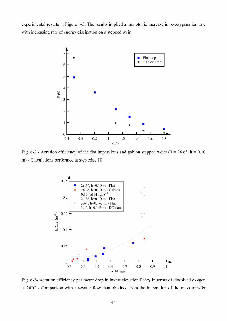
44
experimental results in Figure 6-3. The results implied a monotonic increase in re-oxygenation rate
with increasing rate of energy dissipation on a stepped weir.
dc/h
E (
%)
0.4 0.6 0.8 1 1.2 1.4 1.6 1.80
1
2
3
4
5
6
7Flat stepsGabion steps
Fig. 6-2 - Aeration efficiency of the flat impervious and gabion stepped weirs (θ = 26.6°, h = 0.10
m) - Calculations performed at step edge 10
H/Hmax
E/
z 0 (
m-1
)
0.3 0.4 0.5 0.6 0.7 0.8 0.9 10
0.05
0.1
0.15
0.2
0.2526.6, h=0.10 m - Flat26.6, h=0.10 m - Gabion0.15 (H/Hmax)2.6
21.8, h=0.10 m - Flat3.4 , h=0.143 m - Flat3.4, h=0.143 m - DO data
Fig. 6-3- Aeration efficiency per metre drop in invert elevation E/Δz0 in terms of dissolved oxygen
at 20°C - Comparison with air-water flow data obtained from the integration of the mass transfer
45
equation (TOOMBES and CHANSON 2005, FELDER and CHANSON 2009) and dissolved
oxygen measurements (TOOMBES and CHANSON 2005)
6.3 DISCUSSION
Large specific interface areas were recorded with depth-averaged values up to 200 m-1. The
integration of Fick’s law based upon detailed air-water flow measurements allowed a comparison
between flat impervious and gabion stepped weirs in terms of aeration performances. The results
showed that, for a small discharge, the aeration efficiency was higher on the gabion stepped chute,
whereas, for large discharges, the flat impervious stepped weir was more efficient in terms of
aeration and mass transfer. The latter trend was consistent with the results of BUNG and
SCHLENKHOFF (2010).
A comparison with previous data showed a good agreement for stepped channels with slopes within
3.4° < θ < 26.6°, highlighting a monotonic increase in re-aeration with increasing rate of energy
dissipation.
46
7. CONCLUSION
The hydraulic performances of gabion stepped weirs were investigated experimentally through a
comprehensive physical study based upon a Froude similitude. Three gabion stepped chutes and a
flat impervious stepped chute were tested in a relatively large size facility with a chute slope of
26.6° (1V:2H) and step height of 0.1 m. The gabion stepped chutes consisted of 10 gabion boxes
filled with 14 mm sieved gravels, stacked above the flat impervious stepped chute. For two
configurations, some horizontal step cappings were added. The hydraulic conductivity of the
gabions was tested and the results yielded K 110-1 m/s. For all configurations, detailed
observations were performed on the chute centreline for a range of discharges corresponding to
Reynolds numbers between 3.8×10⁴ and 8.7×10⁵.
Some detailed visual observations were carried out for all stepped configurations. On the gabion
stepped chutes, a porous regime was observed for the smallest discharges: there was no overflow
and the water seeped through the gabions. For larger discharges, the main overflow regimes
included the nappe, transition and skimming flows with increasing discharges. The interactions
between seepage flow and overflow were functions of the discharge, gabion configuration and flow
regime. They resulted in a modification of the step cavity flow and recirculation patterns. On all
gabion stepped weirs, some strong interaction between the cavity flow and upstream gabion was
observed, as well some bubbly flow motion inside the gabions. The position of the inception point
of free-surface aeration was close on all four stepped configurations for a given discharge, although
slightly further downstream on the gabion and fully-capped stepped chutes.
Some detailed air-water flow measurements were conducted on all step edges downstream of the
inception point of free-surface aeration. The results showed comparable trends for all stepped weirs,
although with some quantitative differences. Overall the gabion stepped chute was less aerated and
the characteristic air-water flow height Y90 was lower than on all other stepped configurations for
an identical flow rate. The bubble count rate and turbulence intensity were also slightly lower on the
gabions stepped weir. In skimming flows, larger velocities were measured at the downstream end of
the gabion stepped chute. The air-water properties of the capped and fully-capped gabion stepped
weirs were typically between the flat impervious and gabion stepped chute flow properties.
The rate of energy dissipation, residual head and equivalent Darcy-Weisbach friction factor were
calculated based upon the air-water flow properties. For low discharges corresponding to nappe
flow regime, the gabion stepped configuration was the most efficient in terms of energy dissipation,
possibly because of the significant proportion of seepage flow rate. In skimming flows, on the other
hand, the energy dissipation rate on the gabion stepped weir was the lowest and the highest rate of
energy dissipation was observed on the flat impervious stepped chute. The Darcy-Weisbach friction
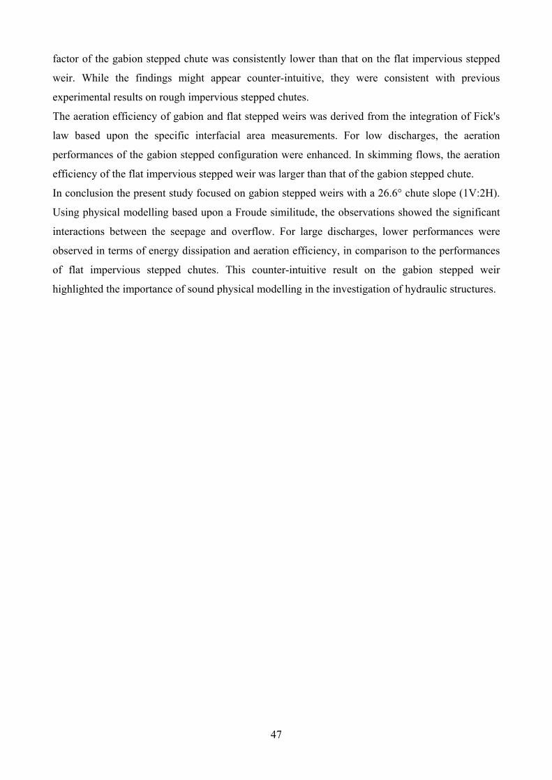
47
factor of the gabion stepped chute was consistently lower than that on the flat impervious stepped
weir. While the findings might appear counter-intuitive, they were consistent with previous
experimental results on rough impervious stepped chutes.
The aeration efficiency of gabion and flat stepped weirs was derived from the integration of Fick's
law based upon the specific interfacial area measurements. For low discharges, the aeration
performances of the gabion stepped configuration were enhanced. In skimming flows, the aeration
efficiency of the flat impervious stepped weir was larger than that of the gabion stepped chute.
In conclusion the present study focused on gabion stepped weirs with a 26.6° chute slope (1V:2H).
Using physical modelling based upon a Froude similitude, the observations showed the significant
interactions between the seepage and overflow. For large discharges, lower performances were
observed in terms of energy dissipation and aeration efficiency, in comparison to the performances
of flat impervious stepped chutes. This counter-intuitive result on the gabion stepped weir
highlighted the importance of sound physical modelling in the investigation of hydraulic structures.

48
8. ACKNOWLEDGEMENTS
The authors thank Professor Daniel BUNG (FH Aachen University of Applied Sciences, Germany)
for his expert review and inputs. The exchanges with Professor Jim KELLS (University of
Saskatchewan, Canada) are acknowledged
The authors acknowledge all the people who assisted with the large-scale experiments and the
technical staff of the School of Civil Engineering at the University of Queensland, in particular
JasonVAN DER GEVEL and Stewart MATTHEWS. The financial support of the Australian
Research Council (Grant DP120100481) is acknowledged.
A-1
APPENDIX A - PHOTOGRAPHS OF STEPPED SPILLWAYS CONFIGURATION AND FLOW PATTERNS
A.1 - PRESENTATION
Visual observations were carried out for all stepped configurations for a wide range of discharges
from 0.005 m3/s to 0.114 m3/s, corresponding to Reynolds numbers between 3.54104 and
8.78105. Table A-1 presents the experimental flow conditions that were investigated during the
project.
This appendix shows a detailed photographic documentation of the experiments. Paragraph A.2
shows the configurations of the stepped spillways facility. In section A.3 a photographic review of
the flow regimes is presented for each configuration and for a wide range of discharges. The flow
patterns observed for each configuration are presented in section A.4 for various discharges.
Table A-1 - Experimental conditions for visual observations of the flow patterns on the stepped
spillway model configurations (θ = 26.6°, h = 0.10 m)
Config. number
Description Q [m3/s]
dc/h [-]
Re [-]
1 Flat steps configuration
h = 0.10 m θ = 26.6°
0.005 - 0.114 0.2 - 1.7 3.54104 - 8.78105
2 Gabion steps configuration
h = 0.10 m θ = 26.6°
0.005 - 0.114 0.2 - 1.7 3.54104 - 8.78105
3 Capped steps configuration
h = 0.10 m θ = 26.6°
0.005 - 0.114 0.2 - 1.7 3.54104 - 8.78105
4 Fully-capped steps configuration
h = 0.10 m θ = 26.6°
0.005 - 0.114 0.2 - 1.7 3.54104 - 8.78105
Notes: dc: critical flow depth, h: step height, Q: water discharge, Re: Reynolds number defined in
terms of hydraulic diameter, θ: channel slope.
Abbreviations:
PR Porous regime (Seepage)
NA Nappe flow regime
TRA Transitions flow regime
SK Skimming flow regime
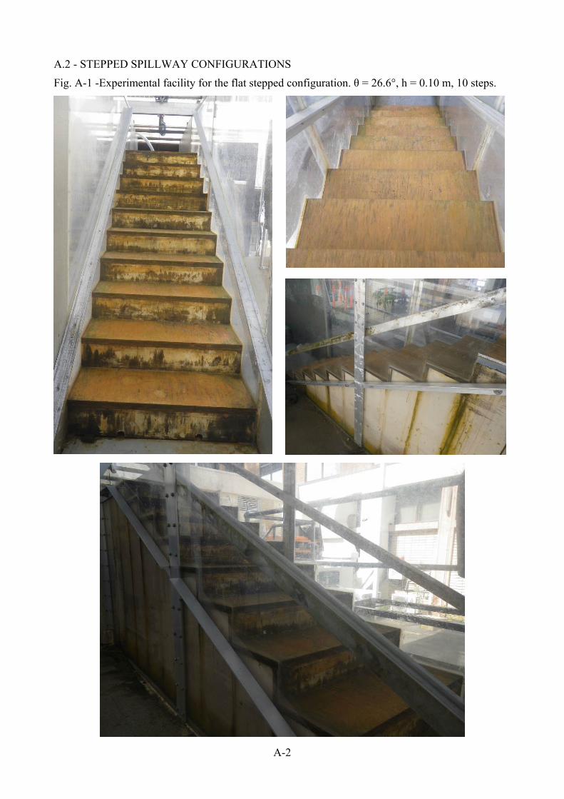
A-2
A.2 - STEPPED SPILLWAY CONFIGURATIONS
Fig. A-1 -Experimental facility for the flat stepped configuration. θ = 26.6°, h = 0.10 m, 10 steps.
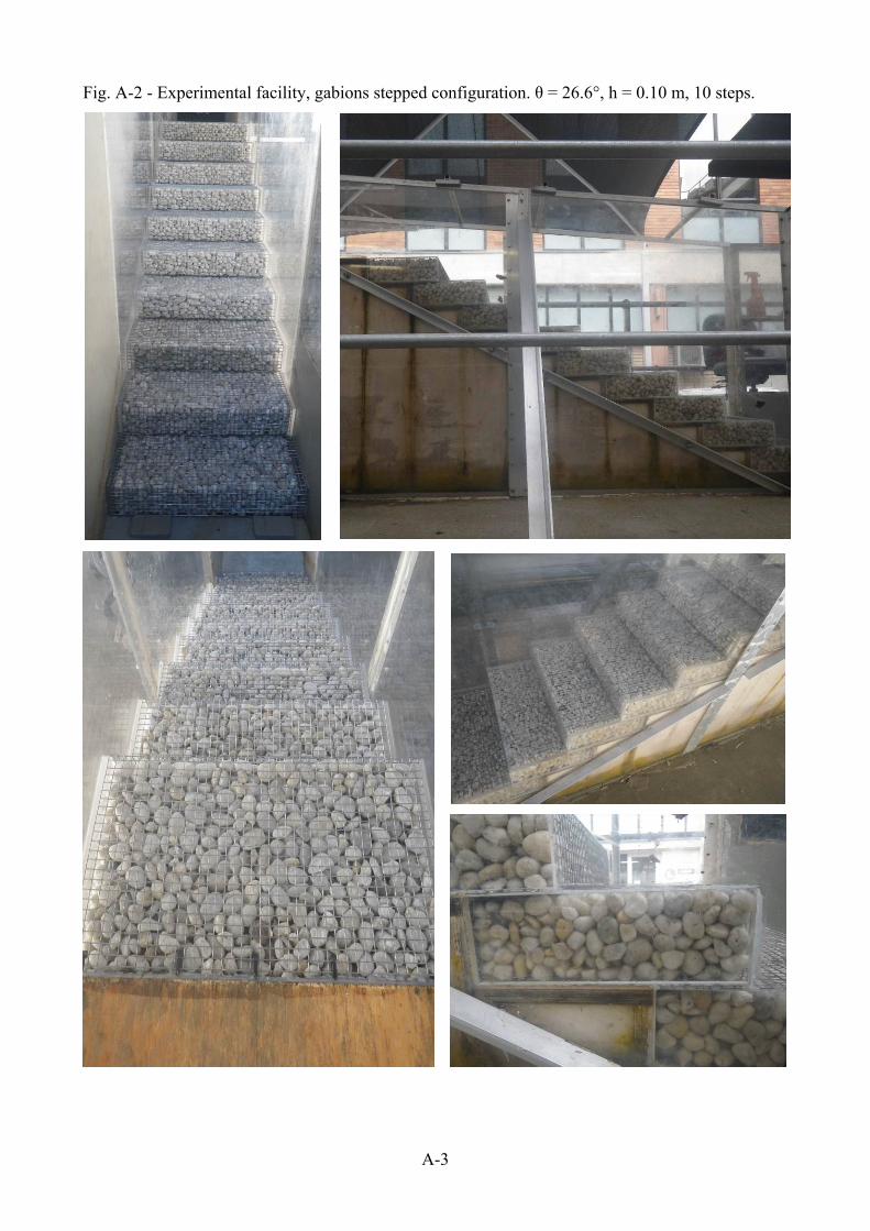
A-3
Fig. A-2 - Experimental facility, gabions stepped configuration. θ = 26.6°, h = 0.10 m, 10 steps.
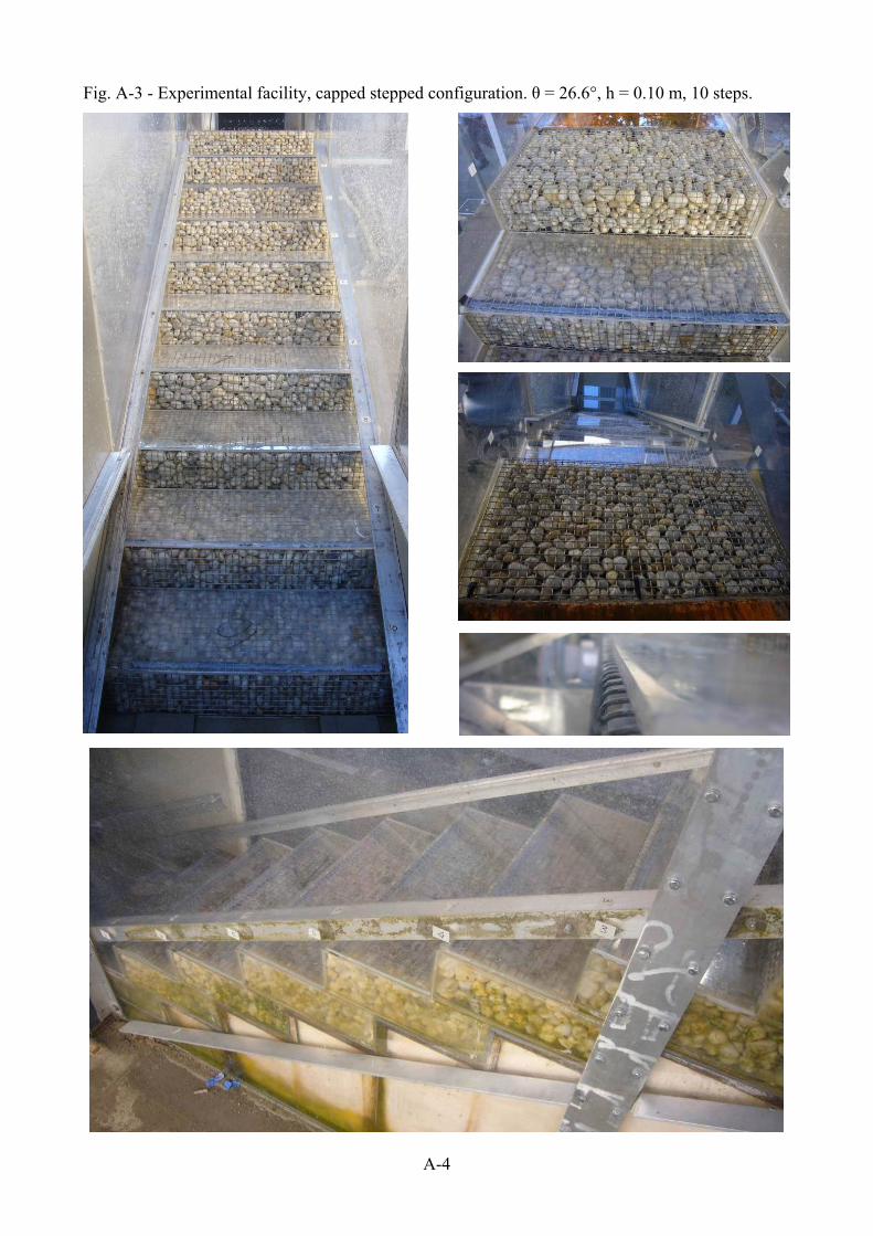
A-4
Fig. A-3 - Experimental facility, capped stepped configuration. θ = 26.6°, h = 0.10 m, 10 steps.

A-5
Fig. A-4 - Experimental facility, fully-capped steps configuration. θ = 26.6°, h = 0.10 m, 10 steps.

A-6
A.3 - FLOW REGIMES
A.3.1 - Flat stepped configuration
Fig. A-5 - Nappe flow regime on the flat stepped configuration (flow direction from left to right)
(A) dc/h = 0.44, Q = 0.015 m3/s, Re = 4.7104 (B) dc/h = 0.44, Q = 0.015 m3/s, Re = 4.7104
(C) dc/h = 0.50, Q = 0.018 m3/s, Re = 1.4105 (D) dc/h = 0.50, Q = 0.018 m3/s, Re = 1.4105
(E) dc/h = 0.50, Q = 0.018 m3/s, Re = 1.4105 (F) dc/h = 0.50, Q = 0.018 m3/s, Re = 1.4105

A-7
Fig. A-6 - Transition flow regime on the flat stepped configuration (flow direction from left to
right)
(A) dc/h = 0.64, Q = 0.027 m3/s, Re = 2.0105 (B) dc/h = 0.64, Q = 0.027 m3/s, Re = 2.0105
(C) dc/h = 0.75, Q = 0.034 m3/s, Re = 2.6105 (D) dc/h = 0.75, Q = 0.034 m3/s, Re = 2.6105
(E) dc/h = 0.80, Q = 0.037 m3/s, Re = 2.8105 (F) dc/h = 0.80, Q = 0.037 m3/s, Re = 2.8105
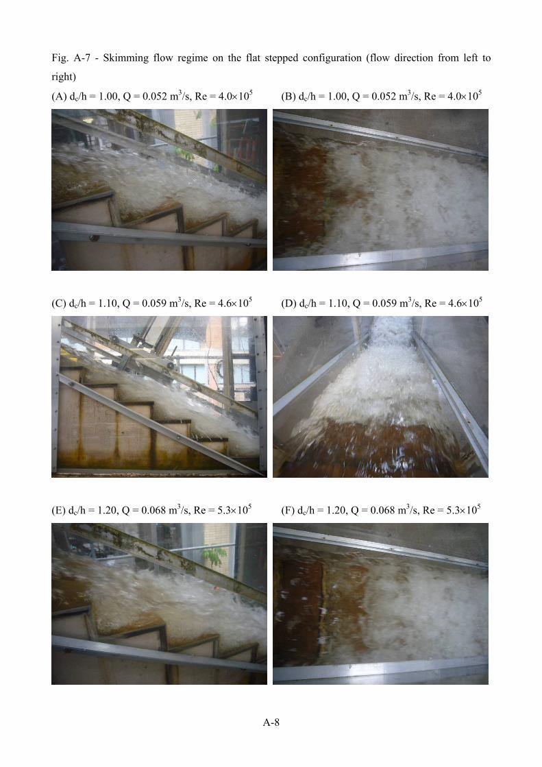
A-8
Fig. A-7 - Skimming flow regime on the flat stepped configuration (flow direction from left to
right)
(A) dc/h = 1.00, Q = 0.052 m3/s, Re = 4.0105 (B) dc/h = 1.00, Q = 0.052 m3/s, Re = 4.0105
(C) dc/h = 1.10, Q = 0.059 m3/s, Re = 4.6105 (D) dc/h = 1.10, Q = 0.059 m3/s, Re = 4.6105
(E) dc/h = 1.20, Q = 0.068 m3/s, Re = 5.3105 (F) dc/h = 1.20, Q = 0.068 m3/s, Re = 5.3105
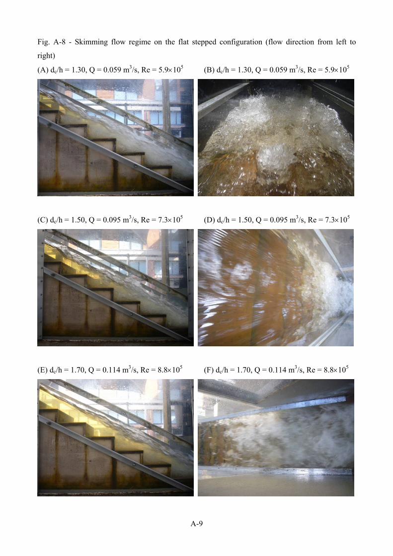
A-9
Fig. A-8 - Skimming flow regime on the flat stepped configuration (flow direction from left to
right)
(A) dc/h = 1.30, Q = 0.059 m3/s, Re = 5.9105 (B) dc/h = 1.30, Q = 0.059 m3/s, Re = 5.9105
(C) dc/h = 1.50, Q = 0.095 m3/s, Re = 7.3105 (D) dc/h = 1.50, Q = 0.095 m3/s, Re = 7.3105
(E) dc/h = 1.70, Q = 0.114 m3/s, Re = 8.8105 (F) dc/h = 1.70, Q = 0.114 m3/s, Re = 8.8105
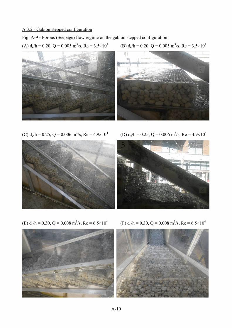
A-10
A.3.2 - Gabion stepped configuration
Fig. A-9 - Porous (Seepage) flow regime on the gabion stepped configuration
(A) dc/h = 0.20, Q = 0.005 m3/s, Re = 3.5104 (B) dc/h = 0.20, Q = 0.005 m3/s, Re = 3.5104
(C) dc/h = 0.25, Q = 0.006 m3/s, Re = 4.9104 (D) dc/h = 0.25, Q = 0.006 m3/s, Re = 4.9104
(E) dc/h = 0.30, Q = 0.008 m3/s, Re = 6.5104 (F) dc/h = 0.30, Q = 0.008 m3/s, Re = 6.5104
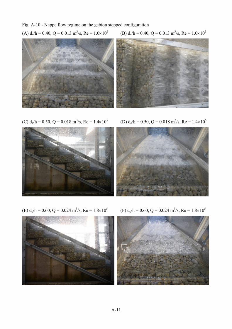
A-11
Fig. A-10 - Nappe flow regime on the gabion stepped configuration
(A) dc/h = 0.40, Q = 0.013 m3/s, Re = 1.0105 (B) dc/h = 0.40, Q = 0.013 m3/s, Re = 1.0105
(C) dc/h = 0.50, Q = 0.018 m3/s, Re = 1.4105 (D) dc/h = 0.50, Q = 0.018 m3/s, Re = 1.4105
(E) dc/h = 0.60, Q = 0.024 m3/s, Re = 1.8105 (F) dc/h = 0.60, Q = 0.024 m3/s, Re = 1.8105
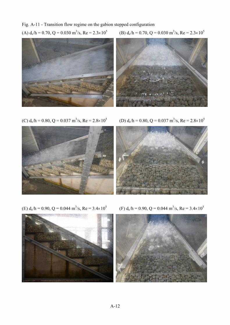
A-12
Fig. A-11 - Transition flow regime on the gabion stepped configuration
(A) dc/h = 0.70, Q = 0.030 m3/s, Re = 2.3105 (B) dc/h = 0.70, Q = 0.030 m3/s, Re = 2.3105
(C) dc/h = 0.80, Q = 0.037 m3/s, Re = 2.8105 (D) dc/h = 0.80, Q = 0.037 m3/s, Re = 2.8105
(E) dc/h = 0.90, Q = 0.044 m3/s, Re = 3.4105 (F) dc/h = 0.90, Q = 0.044 m3/s, Re = 3.4105
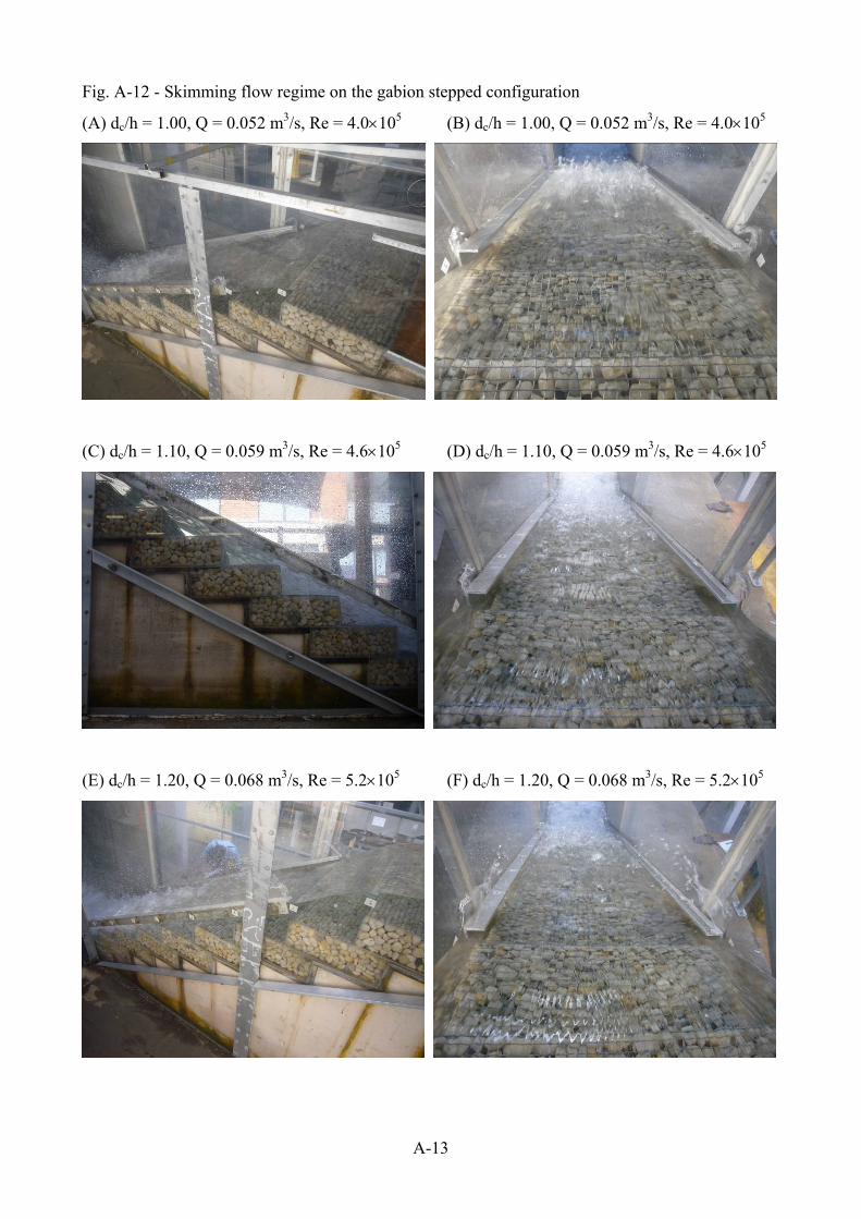
A-13
Fig. A-12 - Skimming flow regime on the gabion stepped configuration
(A) dc/h = 1.00, Q = 0.052 m3/s, Re = 4.0105 (B) dc/h = 1.00, Q = 0.052 m3/s, Re = 4.0105
(C) dc/h = 1.10, Q = 0.059 m3/s, Re = 4.6105 (D) dc/h = 1.10, Q = 0.059 m3/s, Re = 4.6105
(E) dc/h = 1.20, Q = 0.068 m3/s, Re = 5.2105 (F) dc/h = 1.20, Q = 0.068 m3/s, Re = 5.2105
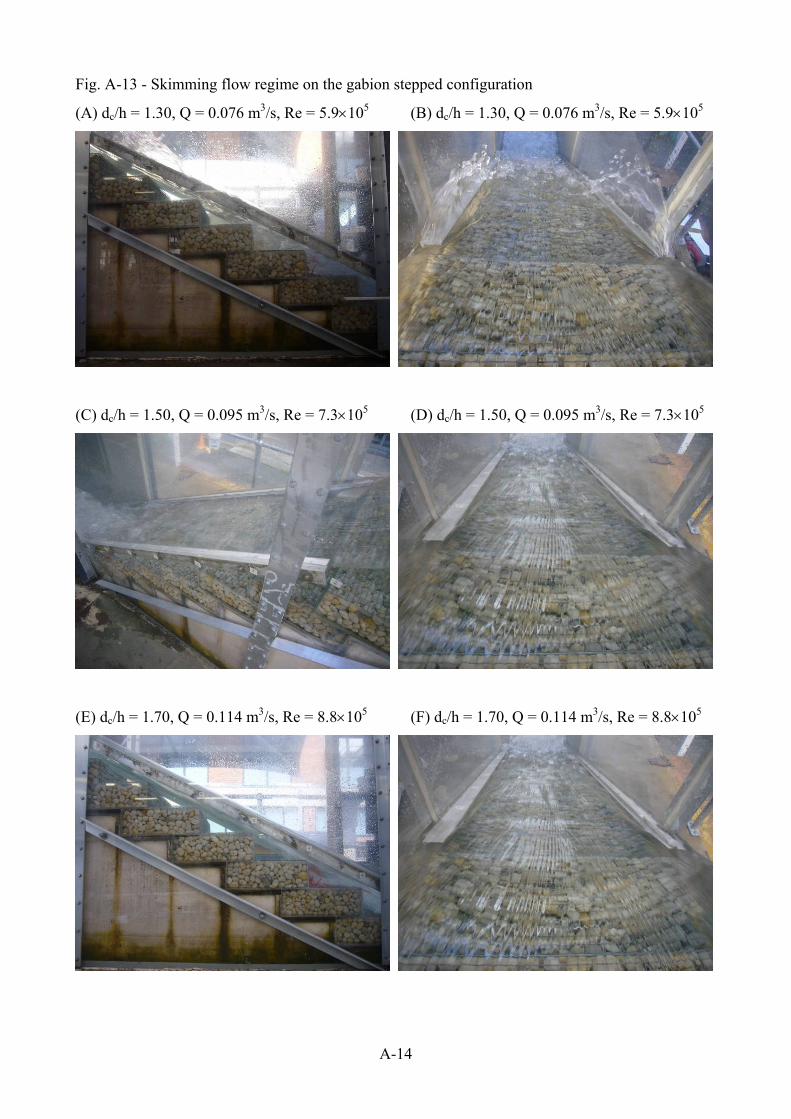
A-14
Fig. A-13 - Skimming flow regime on the gabion stepped configuration
(A) dc/h = 1.30, Q = 0.076 m3/s, Re = 5.9105 (B) dc/h = 1.30, Q = 0.076 m3/s, Re = 5.9105
(C) dc/h = 1.50, Q = 0.095 m3/s, Re = 7.3105 (D) dc/h = 1.50, Q = 0.095 m3/s, Re = 7.3105
(E) dc/h = 1.70, Q = 0.114 m3/s, Re = 8.8105 (F) dc/h = 1.70, Q = 0.114 m3/s, Re = 8.8105

A-15
A.3.3 - Capped stepped configuration
Fig. A-14 - Porous (Seepage) flow regime on the capped stepped configuration
(A) dc/h = 0.20, Q = 0.005 m3/s, Re = 3.5104 (B) dc/h = 0.20, Q = 0.005 m3/s, Re = 3.5104
(C) dc/h = 0.20, Q = 0.005 m3/s, Re = 3.5104 (D) dc/h = 0.20, Q = 0.005 m3/s, Re = 3.5104
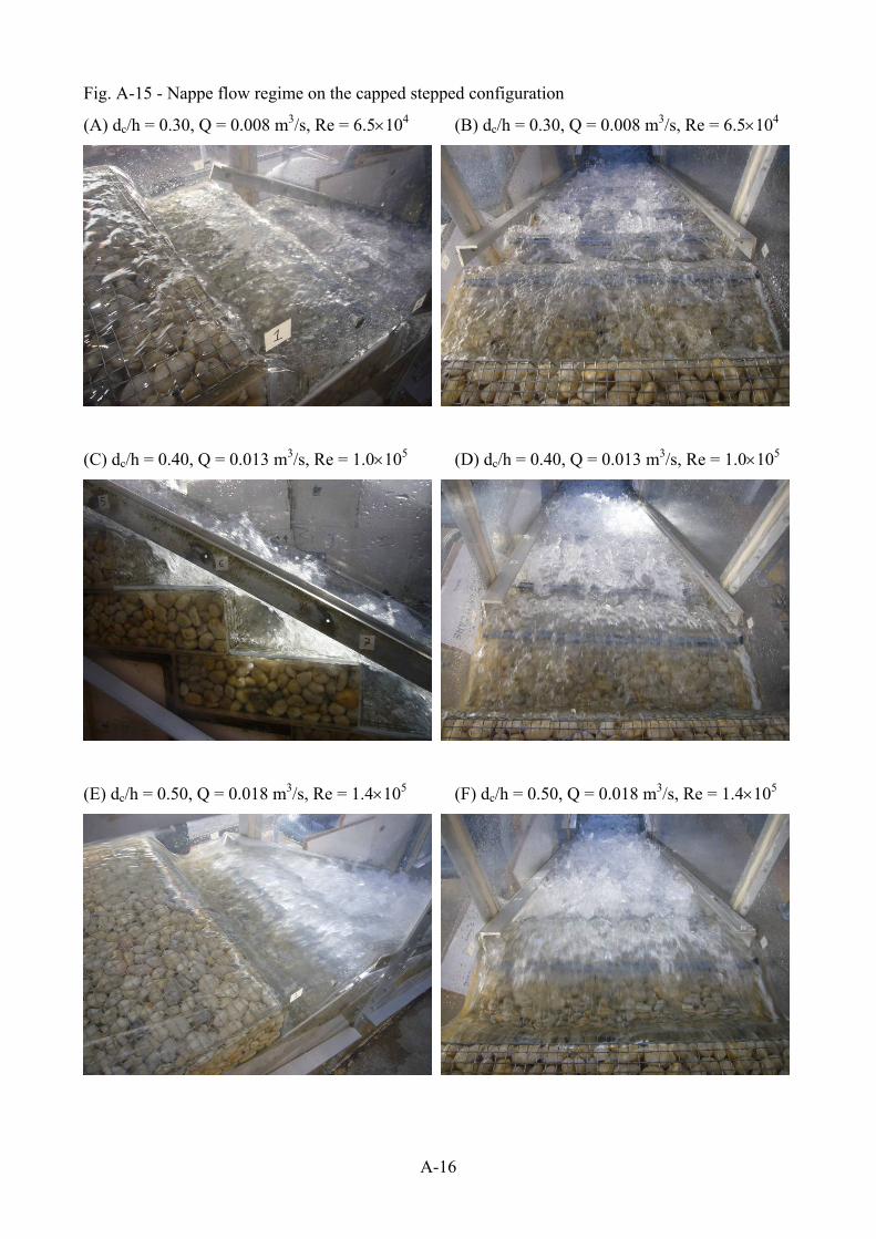
A-16
Fig. A-15 - Nappe flow regime on the capped stepped configuration
(A) dc/h = 0.30, Q = 0.008 m3/s, Re = 6.5104 (B) dc/h = 0.30, Q = 0.008 m3/s, Re = 6.5104
(C) dc/h = 0.40, Q = 0.013 m3/s, Re = 1.0105 (D) dc/h = 0.40, Q = 0.013 m3/s, Re = 1.0105
(E) dc/h = 0.50, Q = 0.018 m3/s, Re = 1.4105 (F) dc/h = 0.50, Q = 0.018 m3/s, Re = 1.4105
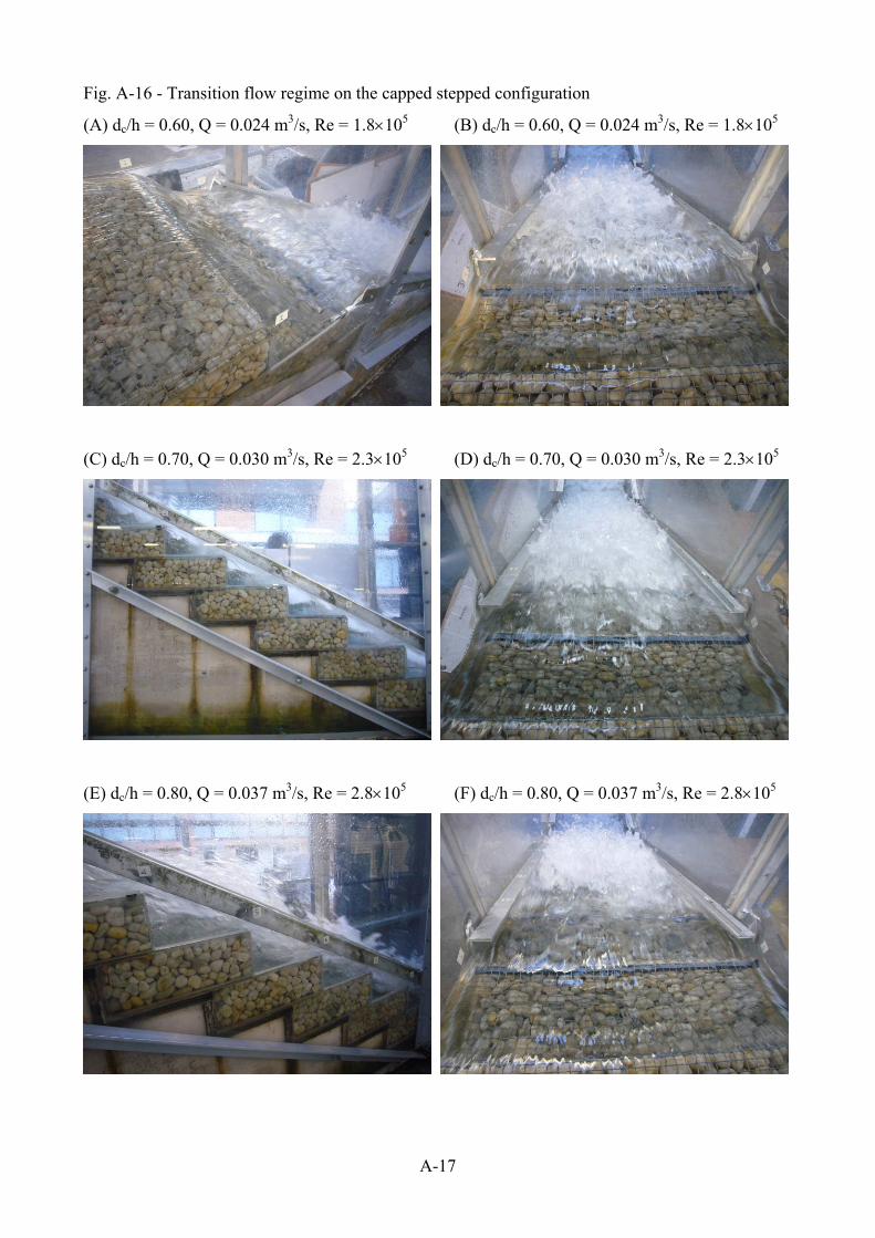
A-17
Fig. A-16 - Transition flow regime on the capped stepped configuration
(A) dc/h = 0.60, Q = 0.024 m3/s, Re = 1.8105 (B) dc/h = 0.60, Q = 0.024 m3/s, Re = 1.8105
(C) dc/h = 0.70, Q = 0.030 m3/s, Re = 2.3105 (D) dc/h = 0.70, Q = 0.030 m3/s, Re = 2.3105
(E) dc/h = 0.80, Q = 0.037 m3/s, Re = 2.8105 (F) dc/h = 0.80, Q = 0.037 m3/s, Re = 2.8105
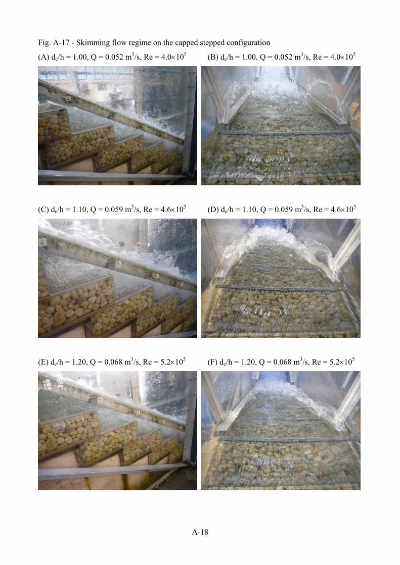
A-18
Fig. A-17 - Skimming flow regime on the capped stepped configuration
(A) dc/h = 1.00, Q = 0.052 m3/s, Re = 4.0105 (B) dc/h = 1.00, Q = 0.052 m3/s, Re = 4.0105
(C) dc/h = 1.10, Q = 0.059 m3/s, Re = 4.6105 (D) dc/h = 1.10, Q = 0.059 m3/s, Re = 4.6105
(E) dc/h = 1.20, Q = 0.068 m3/s, Re = 5.2105 (F) dc/h = 1.20, Q = 0.068 m3/s, Re = 5.2105
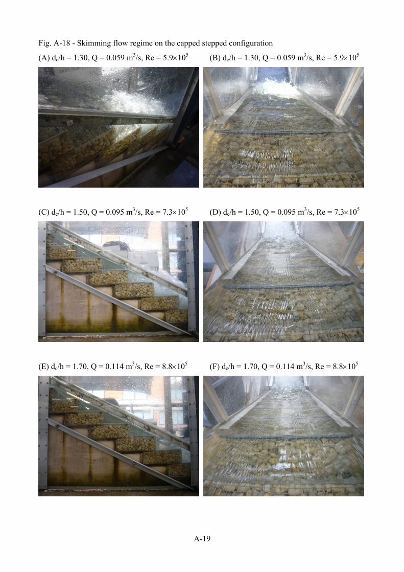
A-19
Fig. A-18 - Skimming flow regime on the capped stepped configuration
(A) dc/h = 1.30, Q = 0.059 m3/s, Re = 5.9105 (B) dc/h = 1.30, Q = 0.059 m3/s, Re = 5.9105
(C) dc/h = 1.50, Q = 0.095 m3/s, Re = 7.3105 (D) dc/h = 1.50, Q = 0.095 m3/s, Re = 7.3105
(E) dc/h = 1.70, Q = 0.114 m3/s, Re = 8.8105 (F) dc/h = 1.70, Q = 0.114 m3/s, Re = 8.8105
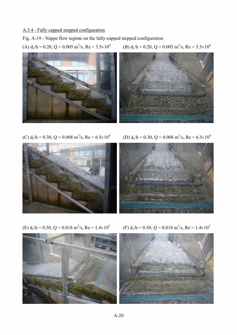
A-20
A.3.4 - Fully capped stepped configuration
Fig. A-19 - Nappe flow regime on the fully-capped stepped configuration
(A) dc/h = 0.20, Q = 0.005 m3/s, Re = 3.5104 (B) dc/h = 0.20, Q = 0.005 m3/s, Re = 3.5104
(C) dc/h = 0.30, Q = 0.008 m3/s, Re = 6.5104 (D) dc/h = 0.30, Q = 0.008 m3/s, Re = 6.5104
(E) dc/h = 0.50, Q = 0.018 m3/s, Re = 1.4105 (F) dc/h = 0.50, Q = 0.018 m3/s, Re = 1.4105

A-21
Fig. A-20 - Transition flow regime on the fully-capped stepped configuration
(A) dc/h = 0.60, Q = 0.024 m3/s, Re = 1.8105 (B) dc/h = 0.60, Q = 0.024 m3/s, Re = 1.8105
(C) dc/h = 0.70, Q = 0.030 m3/s, Re = 2.3105 (D) dc/h = 0.70, Q = 0.030 m3/s, Re = 2.3105
(E) dc/h = 0.80, Q = 0.037 m3/s, Re = 2.8105 (F) dc/h = 0.80, Q = 0.037 m3/s, Re = 2.8105

A-22
Fig. A-21 - Skimming flow regime on the fully-capped stepped configuration
(A) dc/h = 1.00, Q = 0.052 m3/s, Re = 4.0105 (B) dc/h = 1.00, Q = 0.052 m3/s, Re = 4.0105
(C) dc/h = 1.10, Q = 0.059 m3/s, Re = 4.6105 (D) dc/h = 1.10, Q = 0.059 m3/s, Re = 4.6105
(E) dc/h = 1.20, Q = 0.068 m3/s, Re = 5.2105 (F) dc/h = 1.20, Q = 0.068 m3/s, Re = 5.2105
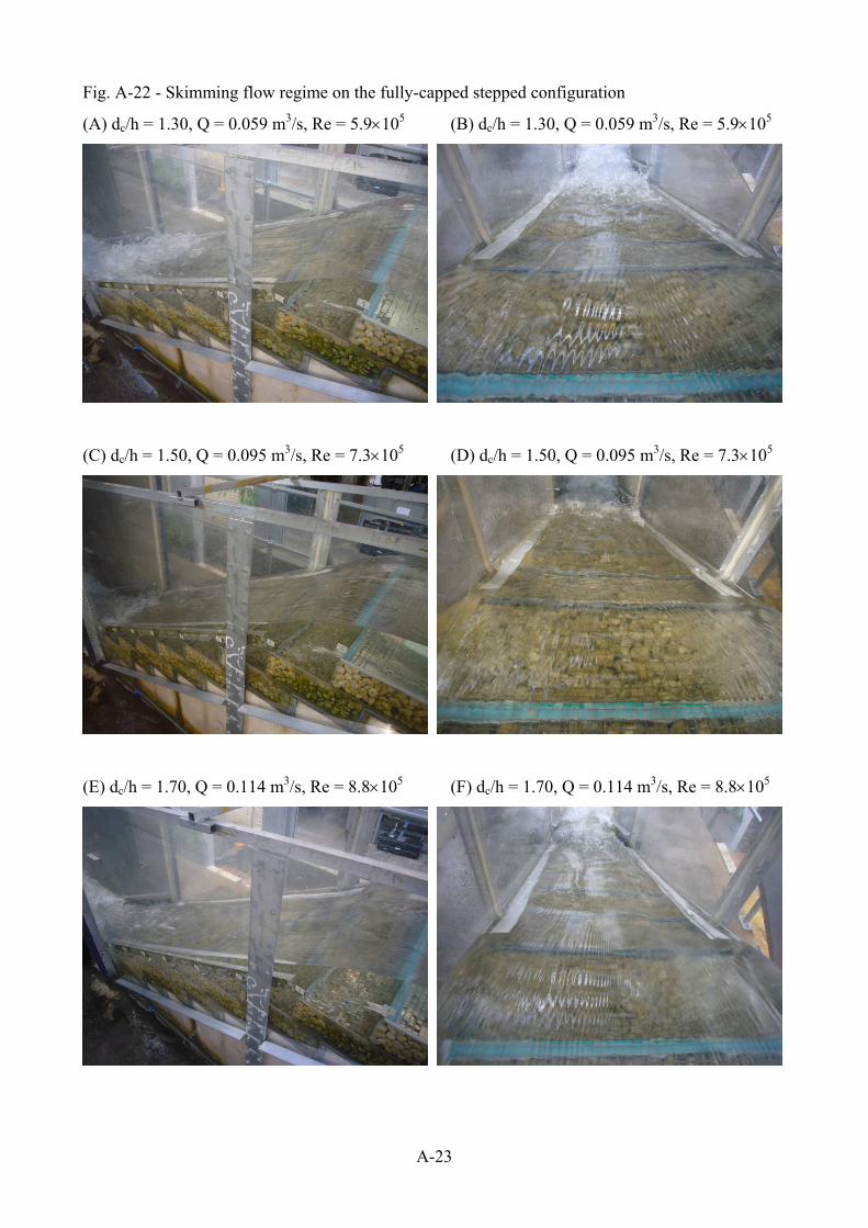
A-23
Fig. A-22 - Skimming flow regime on the fully-capped stepped configuration
(A) dc/h = 1.30, Q = 0.059 m3/s, Re = 5.9105 (B) dc/h = 1.30, Q = 0.059 m3/s, Re = 5.9105
(C) dc/h = 1.50, Q = 0.095 m3/s, Re = 7.3105 (D) dc/h = 1.50, Q = 0.095 m3/s, Re = 7.3105
(E) dc/h = 1.70, Q = 0.114 m3/s, Re = 8.8105 (F) dc/h = 1.70, Q = 0.114 m3/s, Re = 8.8105
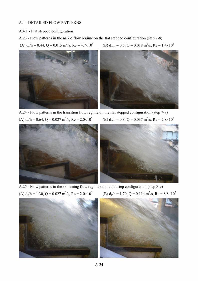
A-24
A.4 - DETAILED FLOW PATTERNS
A.4.1 - Flat stepped configuration
A.23 - Flow patterns in the nappe flow regime on the flat stepped configuration (step 7-8)
(A) dc/h = 0.44, Q = 0.015 m3/s, Re = 4.7104 (B) dc/h = 0.5, Q = 0.018 m3/s, Re = 1.4105
A.24 - Flow patterns in the transition flow regime on the flat stepped configuration (step 7-8)
(A) dc/h = 0.64, Q = 0.027 m3/s, Re = 2.0105 (B) dc/h = 0.8, Q = 0.037 m3/s, Re = 2.8105
A.25 - Flow patterns in the skimming flow regime on the flat step configuration (step 8-9)
(A) dc/h = 1.30, Q = 0.027 m3/s, Re = 2.0105 (B) dc/h = 1.70, Q = 0.114 m3/s, Re = 8.8105
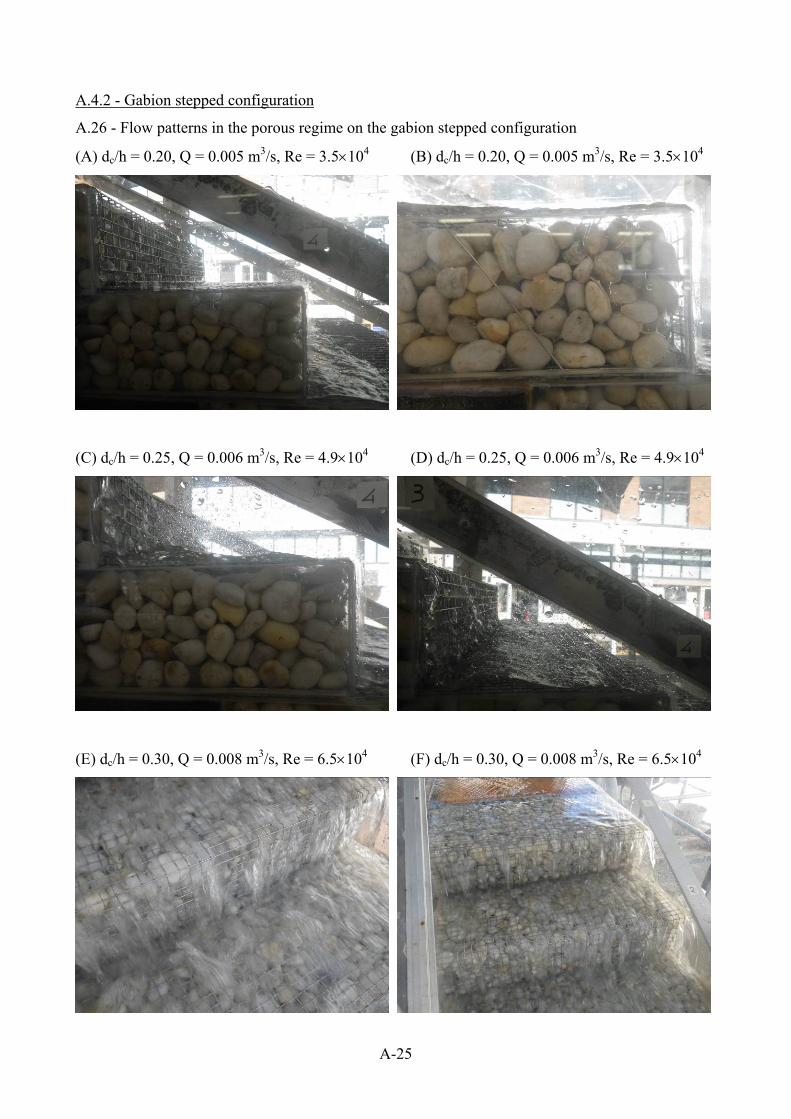
A-25
A.4.2 - Gabion stepped configuration
A.26 - Flow patterns in the porous regime on the gabion stepped configuration
(A) dc/h = 0.20, Q = 0.005 m3/s, Re = 3.5104 (B) dc/h = 0.20, Q = 0.005 m3/s, Re = 3.5104
(C) dc/h = 0.25, Q = 0.006 m3/s, Re = 4.9104 (D) dc/h = 0.25, Q = 0.006 m3/s, Re = 4.9104
(E) dc/h = 0.30, Q = 0.008 m3/s, Re = 6.5104 (F) dc/h = 0.30, Q = 0.008 m3/s, Re = 6.5104
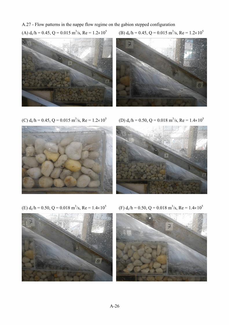
A-26
A.27 - Flow patterns in the nappe flow regime on the gabion stepped configuration
(A) dc/h = 0.45, Q = 0.015 m3/s, Re = 1.2105 (B) dc/h = 0.45, Q = 0.015 m3/s, Re = 1.2105
(C) dc/h = 0.45, Q = 0.015 m3/s, Re = 1.2105 (D) dc/h = 0.50, Q = 0.018 m3/s, Re = 1.4105
(E) dc/h = 0.50, Q = 0.018 m3/s, Re = 1.4105 (F) dc/h = 0.50, Q = 0.018 m3/s, Re = 1.4105
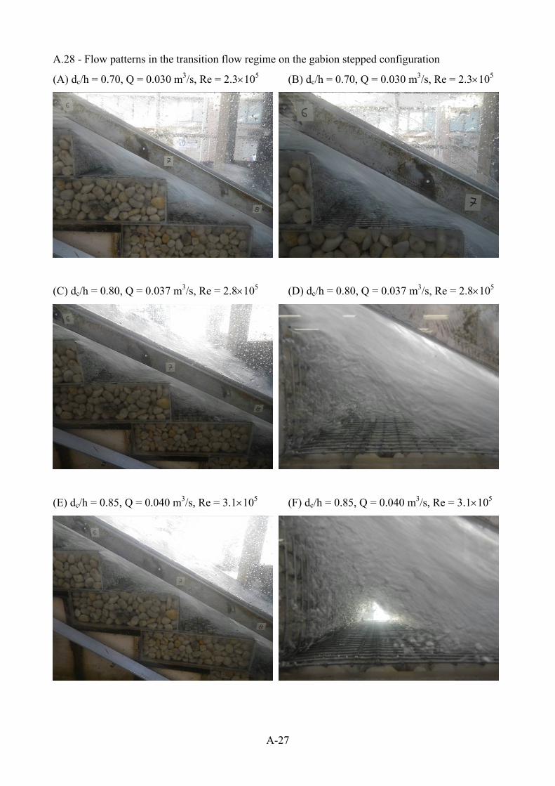
A-27
A.28 - Flow patterns in the transition flow regime on the gabion stepped configuration
(A) dc/h = 0.70, Q = 0.030 m3/s, Re = 2.3105 (B) dc/h = 0.70, Q = 0.030 m3/s, Re = 2.3105
(C) dc/h = 0.80, Q = 0.037 m3/s, Re = 2.8105 (D) dc/h = 0.80, Q = 0.037 m3/s, Re = 2.8105
(E) dc/h = 0.85, Q = 0.040 m3/s, Re = 3.1105 (F) dc/h = 0.85, Q = 0.040 m3/s, Re = 3.1105

A-28
A.29 - Flow patterns in the skimming flow regime on the gabion stepped configuration
(A) dc/h = 1.1, Q = 0.059 m3/s, Re = 4.6105 (B) dc/h = 1.1, Q = 0.059 m3/s, Re = 4.6105
(C) dc/h = 1.20, Q = 0.068 m3/s, Re = 5.2105 (D) dc/h = 1.30, Q = 0.076 m3/s, Re = 5.9105
(E) dc/h = 1.40, Q = 0.085 m3/s, Re = 6.6105 (F) dc/h = 1.50, Q = 0.095 m3/s, Re = 7.3105
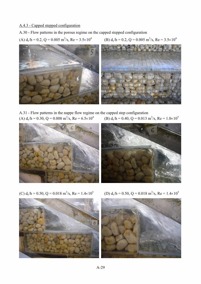
A-29
A.4.3 - Capped stepped configuration
A.30 - Flow patterns in the porous regime on the capped stepped configuration
(A) dc/h = 0.2, Q = 0.005 m3/s, Re = 3.5104 (B) dc/h = 0.2, Q = 0.005 m3/s, Re = 3.5104
A.31 - Flow patterns in the nappe flow regime on the capped step configuration
(A) dc/h = 0.30, Q = 0.008 m3/s, Re = 6.5104 (B) dc/h = 0.40, Q = 0.013 m3/s, Re = 1.0105
(C) dc/h = 0.50, Q = 0.018 m3/s, Re = 1.4105 (D) dc/h = 0.50, Q = 0.018 m3/s, Re = 1.4105
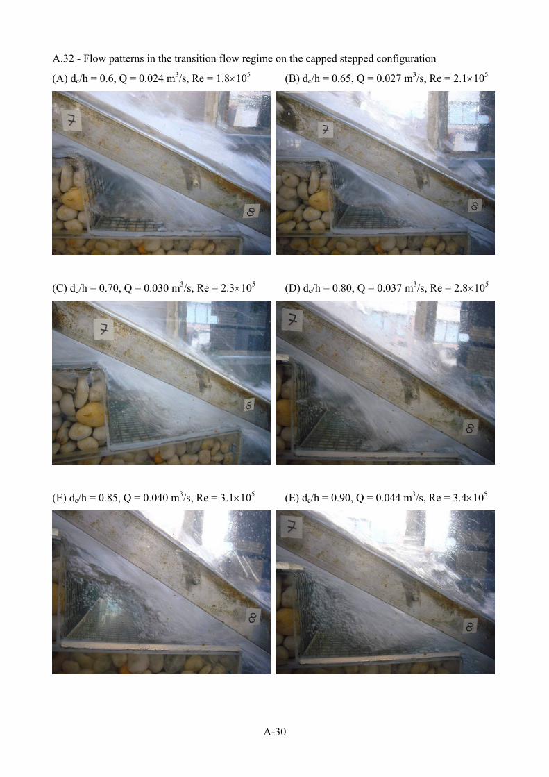
A-30
A.32 - Flow patterns in the transition flow regime on the capped stepped configuration
(A) dc/h = 0.6, Q = 0.024 m3/s, Re = 1.8105 (B) dc/h = 0.65, Q = 0.027 m3/s, Re = 2.1105
(C) dc/h = 0.70, Q = 0.030 m3/s, Re = 2.3105 (D) dc/h = 0.80, Q = 0.037 m3/s, Re = 2.8105
(E) dc/h = 0.85, Q = 0.040 m3/s, Re = 3.1105 (E) dc/h = 0.90, Q = 0.044 m3/s, Re = 3.4105
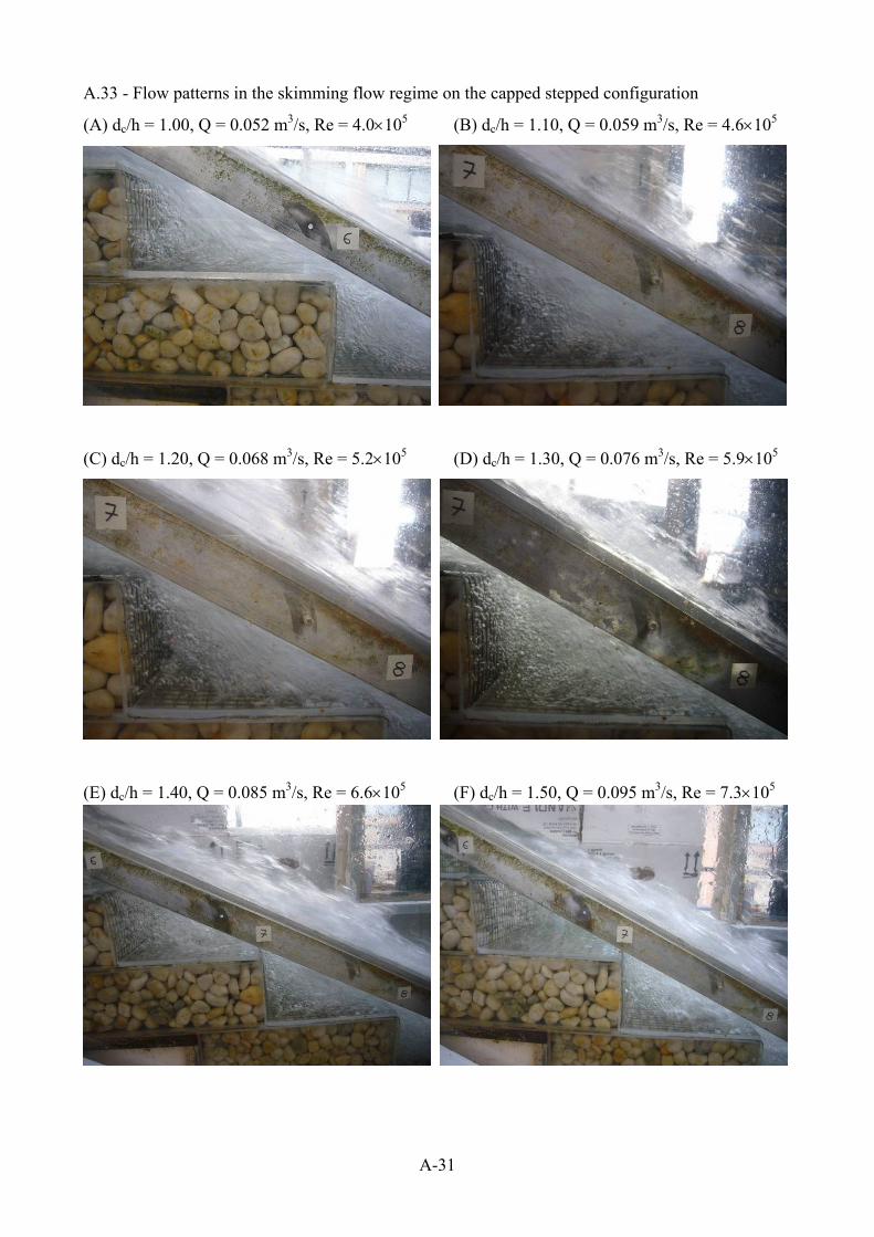
A-31
A.33 - Flow patterns in the skimming flow regime on the capped stepped configuration
(A) dc/h = 1.00, Q = 0.052 m3/s, Re = 4.0105 (B) dc/h = 1.10, Q = 0.059 m3/s, Re = 4.6105
(C) dc/h = 1.20, Q = 0.068 m3/s, Re = 5.2105 (D) dc/h = 1.30, Q = 0.076 m3/s, Re = 5.9105
(E) dc/h = 1.40, Q = 0.085 m3/s, Re = 6.6105 (F) dc/h = 1.50, Q = 0.095 m3/s, Re = 7.3105
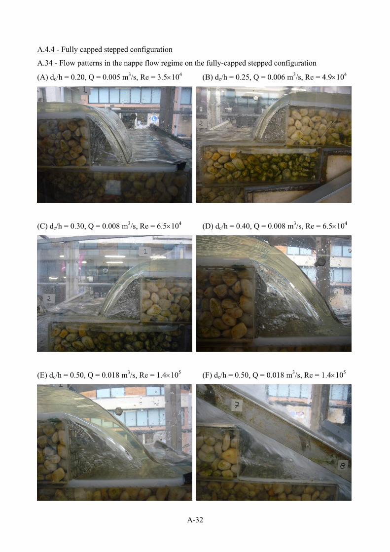
A-32
A.4.4 - Fully capped stepped configuration
A.34 - Flow patterns in the nappe flow regime on the fully-capped stepped configuration
(A) dc/h = 0.20, Q = 0.005 m3/s, Re = 3.5104 (B) dc/h = 0.25, Q = 0.006 m3/s, Re = 4.9104
(C) dc/h = 0.30, Q = 0.008 m3/s, Re = 6.5104 (D) dc/h = 0.40, Q = 0.008 m3/s, Re = 6.5104
(E) dc/h = 0.50, Q = 0.018 m3/s, Re = 1.4105 (F) dc/h = 0.50, Q = 0.018 m3/s, Re = 1.4105
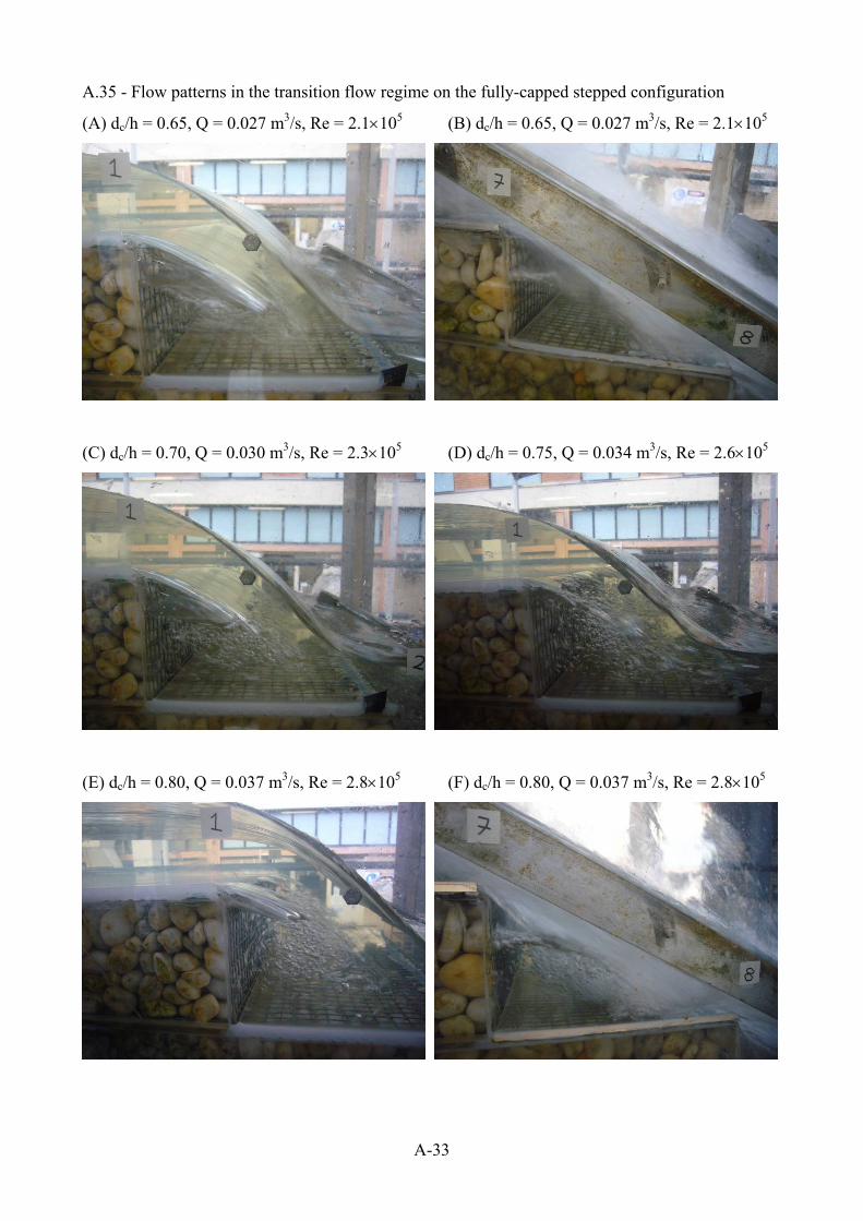
A-33
A.35 - Flow patterns in the transition flow regime on the fully-capped stepped configuration
(A) dc/h = 0.65, Q = 0.027 m3/s, Re = 2.1105 (B) dc/h = 0.65, Q = 0.027 m3/s, Re = 2.1105
(C) dc/h = 0.70, Q = 0.030 m3/s, Re = 2.3105 (D) dc/h = 0.75, Q = 0.034 m3/s, Re = 2.6105
(E) dc/h = 0.80, Q = 0.037 m3/s, Re = 2.8105 (F) dc/h = 0.80, Q = 0.037 m3/s, Re = 2.8105
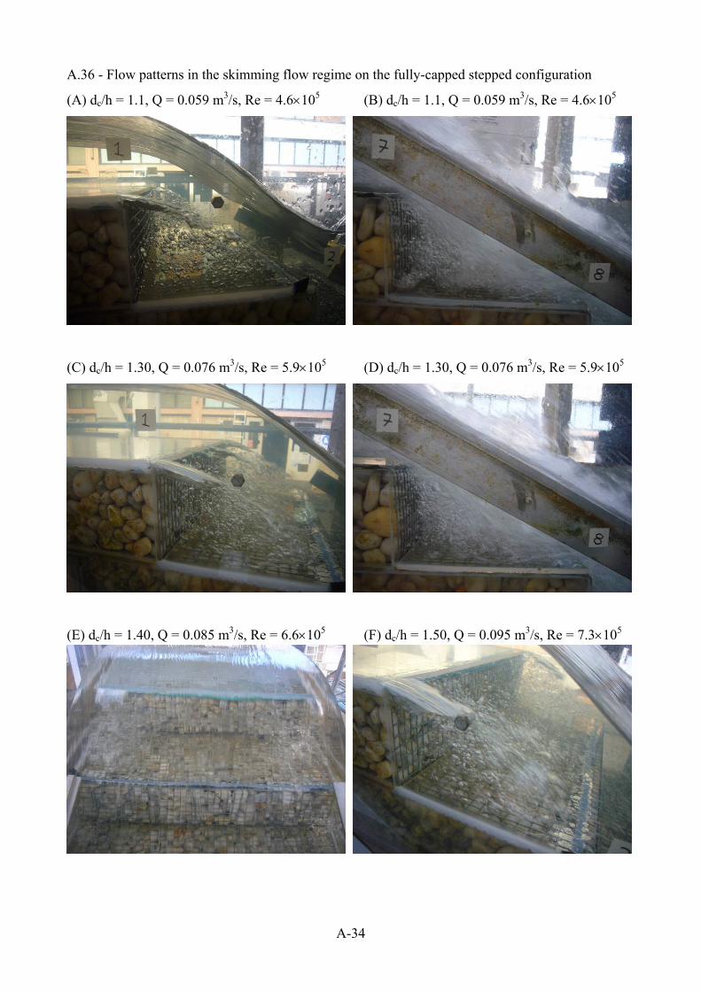
A-34
A.36 - Flow patterns in the skimming flow regime on the fully-capped stepped configuration
(A) dc/h = 1.1, Q = 0.059 m3/s, Re = 4.6105 (B) dc/h = 1.1, Q = 0.059 m3/s, Re = 4.6105
(C) dc/h = 1.30, Q = 0.076 m3/s, Re = 5.9105 (D) dc/h = 1.30, Q = 0.076 m3/s, Re = 5.9105
(E) dc/h = 1.40, Q = 0.085 m3/s, Re = 6.6105 (F) dc/h = 1.50, Q = 0.095 m3/s, Re = 7.3105
B-1
APPENDIX B - SIGNAL PROCESSING AND SENSITIVITY ANALYSIS
B.1 INTRODUCTION
The air water properties were recorded using a double tip conductivity probe. The conductivity
probe detected the difference in conductivity (or resistivity) between the two phases. Section B.2
shows how the main air-water properties were deduced from the raw probe signal. It is known that
the output values of the signal processing depend the sampling duration and frequency. Section B.3
presents a sensitivity analysis of the main signal acquisition parameters and their influence on the
air-water properties.
Notation
C air concentration, defined as the volume of air per unit volume; it is also called void
fraction;
dc critical depth of the flow (m);
F bubble frequency defined as the number of detected air bubbles per unit time; also
called bubble count rate (Hz);
h height of the steps (m);
Q water discharge (m3/s);
R correlation function;
Re Reynolds number defined in terms of hydraulic diameter;
Rxx normalised auto-correlation function;
t time (s);
T time lag (s) for which the cross correlation between the signals is maximum;
T0.5 time lag (s) for which the auto correlation function Rxx(T0.5) = 0.5;
Tu turbulence intensity;
V interfacial velocity (m/s);
y distance measured perpendicular to the pseudo-bottom formed by the step edges (m);
Δx streamwise distance between the probe tips (m);
Δz transversal distance between the probe tips (m);
Ø diameter of the probe sensor (m);
τ0.5 time lag (s) for which the cross correlation function is half of its maximum value.

B-2
B.2 SIGNAL PROCESSING
The operation of conductivity needle probes is based upon the difference in conductivity between
the two phases (air and water) since the resistivity of water is much lower than that of air. A typical
raw signal is presented in Figure B-1.
Fig B-1 - Raw probe signal detected for dc /h = 1.3, Step 10, sampling frequency: 20 kHz, sampling
duration: 45 s.
(A) Raw signal recorded between t = 0 and t = 1 s.
Time
Vol
tage
0 0.1 0.2 0.3 0.4 0.5 0.6 0.7 0.8 0.9 1-1
-0.5
0
0.5
1
1.5
2
2.5
3
3.5
4
4.5
Leading tip Trailing tip
(B) Raw probe signal between t = 0.8 s and t = 0.85 s
Time
Vol
tage
0.8 0.805 0.81 0.815 0.82 0.825 0.83 0.835 0.84 0.845 0.85-1
-0.5
0
0.5
1
1.5
2
2.5
3
3.5
4
4.5
Leading tip Trailing tip
Theoretically the probe signal should be rectangular. But due to the finite size of the tips, the

B-3
wetting/drying time of the tip and the response time of the probe and the electronics, the signal is
not perfectly squared (CHANSON and GONZALEZ 2005). As a result, an air-water threshold is
introduced: e.g., if the value of the signal is greater than 50%, than it is considered water, otherwise
air (Fig. B-2).
Fig B-2 - Sketch of the effect of the air-water threshold in the signal processing analysis
(CHANSON 1995b)
In this study, the void fraction and bubble count rate data were processed using a single threshold
technique and the threshold was set to 50 % of the full air-water voltage range. A sensitivity
analysis was conducted with thresholds between 10 and 90% of the voltage range. The results
showed little effect of the threshold level on air-water flow properties (Appendix B.3). The void
fraction and bubble count rate are defined as:
Air concentration, or void fraction, C, is the proportion of time that the probe tip spent in
contact with air.
The bubble count rate, or bubble frequency, F, is the number of bubbles that the tip of the
probe encounters per second (Hz).
Further information may be obtained using a cross-correlation technique between the leading and
trailing tip signals (e.g. CAIN and WOOD 1981, CROWE et al. 1998). Namely the interfacial
velocity and the turbulence intensity. The time-averaged air-water velocity V is estimated as
T
xV
(B-1)
where Δx is the longitudinal distance between the leading and the trailing tips, and T is time lag for
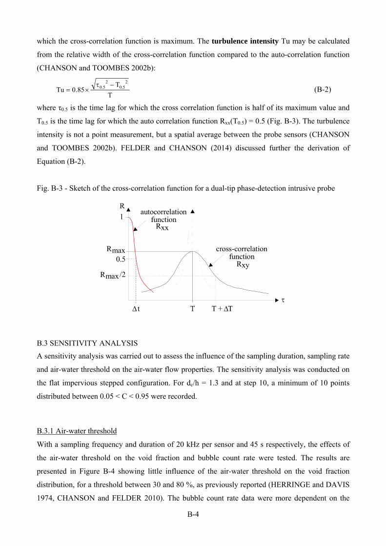
B-4
which the cross-correlation function is maximum. The turbulence intensity Tu may be calculated
from the relative width of the cross-correlation function compared to the auto-correlation function
(CHANSON and TOOMBES 2002b):
T
T85.0Tu
25.0
25.0
(B-2)
where τ0.5 is the time lag for which the cross correlation function is half of its maximum value and
T0.5 is the time lag for which the auto correlation function Rxx(T0.5) = 0.5 (Fig. B-3). The turbulence
intensity is not a point measurement, but a spatial average between the probe sensors (CHANSON
and TOOMBES 2002b). FELDER and CHANSON (2014) discussed further the derivation of
Equation (B-2).
Fig. B-3 - Sketch of the cross-correlation function for a dual-tip phase-detection intrusive probe
B.3 SENSITIVITY ANALYSIS
A sensitivity analysis was carried out to assess the influence of the sampling duration, sampling rate
and air-water threshold on the air-water flow properties. The sensitivity analysis was conducted on
the flat impervious stepped configuration. For dc/h = 1.3 and at step 10, a minimum of 10 points
distributed between 0.05 < C < 0.95 were recorded.
B.3.1 Air-water threshold
With a sampling frequency and duration of 20 kHz per sensor and 45 s respectively, the effects of
the air-water threshold on the void fraction and bubble count rate were tested. The results are
presented in Figure B-4 showing little influence of the air-water threshold on the void fraction
distribution, for a threshold between 30 and 80 %, as previously reported (HERRINGE and DAVIS
1974, CHANSON and FELDER 2010). The bubble count rate data were more dependent on the

B-5
threshold level. Overall the present results justified the selection of a 50 % air-water threshold, as
shown by TOOMBES (2002) and FELDER (2013).
Fig. B-4 - Effect of the air-water threshold on the void fraction and bubble count rate. Sampling
duration 45 s, sampling frequency 20 kHz per sensor, dc/h = 1.3, step 10, Re = 5.87105, Q =
0.0763m3/s
(A) Void Fraction (B) Bubble frequency
Air-Water Threshold [%]
C
0 20 40 60 80 1000
0.1
0.2
0.3
0.4
0.5
0.6
0.7
0.8
0.9
1
y = 22 mmy = 35 mmy = 48 mm
y = 58 mmy = 64 mmy = 74 mm
Air-Water Threshold [%]
F [
Hz]
0 20 40 60 80 1000
20
40
60
80
100
120
140
160
180
200
y = 22 mmy = 35 mmy = 48 mm
y = 58 mmy = 64 mmy = 74 mm
B.3.2 Effect of sampling duration
The raw signal was sampled for 180 s at 20 kHz. The data was analysed with a 50% air-water
threshold. Using smaller non-overlapping segments, the void fraction, bubble count rate, interfacial
velocity and turbulence intensity were calculated for each segment. The results showed that the
sampling duration had no effect on the vertical distributions of void fraction, bubble count rate and
time-averaged interfacial velocity for sampling durations equal to and greater than 20 s (Fig. B-5).
In terms of the turbulence intensity distributions, the sampling duration had to be at least 45 s (Fig.
B-5D). The results were generally in agreement with the results of CHANSON and FELDER
(2010) in skimming flows on a stepped spillway. Herein the selection of a 45 s sampling duration
was thus justified by the results.
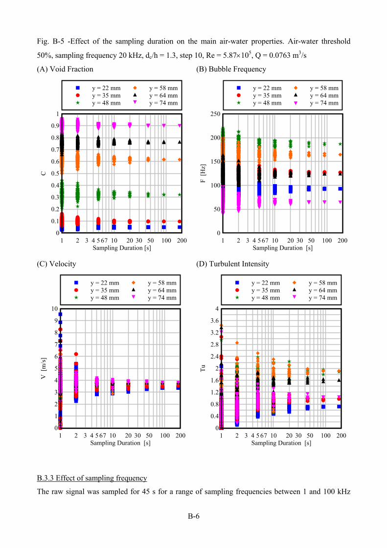
B-6
Fig. B-5 -Effect of the sampling duration on the main air-water properties. Air-water threshold
50%, sampling frequency 20 kHz, dc/h = 1.3, step 10, Re = 5.87105, Q = 0.0763 m3/s
(A) Void Fraction (B) Bubble Frequency
Sampling Duration [s]
C
1 2 3 4 5 67 10 20 30 50 100 2000
0.1
0.2
0.3
0.4
0.5
0.6
0.7
0.8
0.9
1
y = 22 mmy = 35 mmy = 48 mm
y = 58 mmy = 64 mmy = 74 mm
Sampling Duration [s]
F [
Hz]
1 2 3 4 5 67 10 20 30 50 100 2000
50
100
150
200
250
y = 22 mmy = 35 mmy = 48 mm
y = 58 mmy = 64 mmy = 74 mm
(C) Velocity (D) Turbulent Intensity
Sampling Duration [s]
V [
m/s
]
1 2 3 4 5 67 10 20 30 50 100 2000
1
2
3
4
5
6
7
8
9
10
y = 22 mmy = 35 mmy = 48 mm
y = 58 mmy = 64 mmy = 74 mm
Sampling Duration [s]
Tu
1 2 3 4 5 67 10 20 30 50 100 2000
0.4
0.8
1.2
1.6
2
2.4
2.8
3.2
3.6
4
y = 22 mmy = 35 mmy = 48 mm
y = 58 mmy = 64 mmy = 74 mm
B.3.3 Effect of sampling frequency
The raw signal was sampled for 45 s for a range of sampling frequencies between 1 and 100 kHz
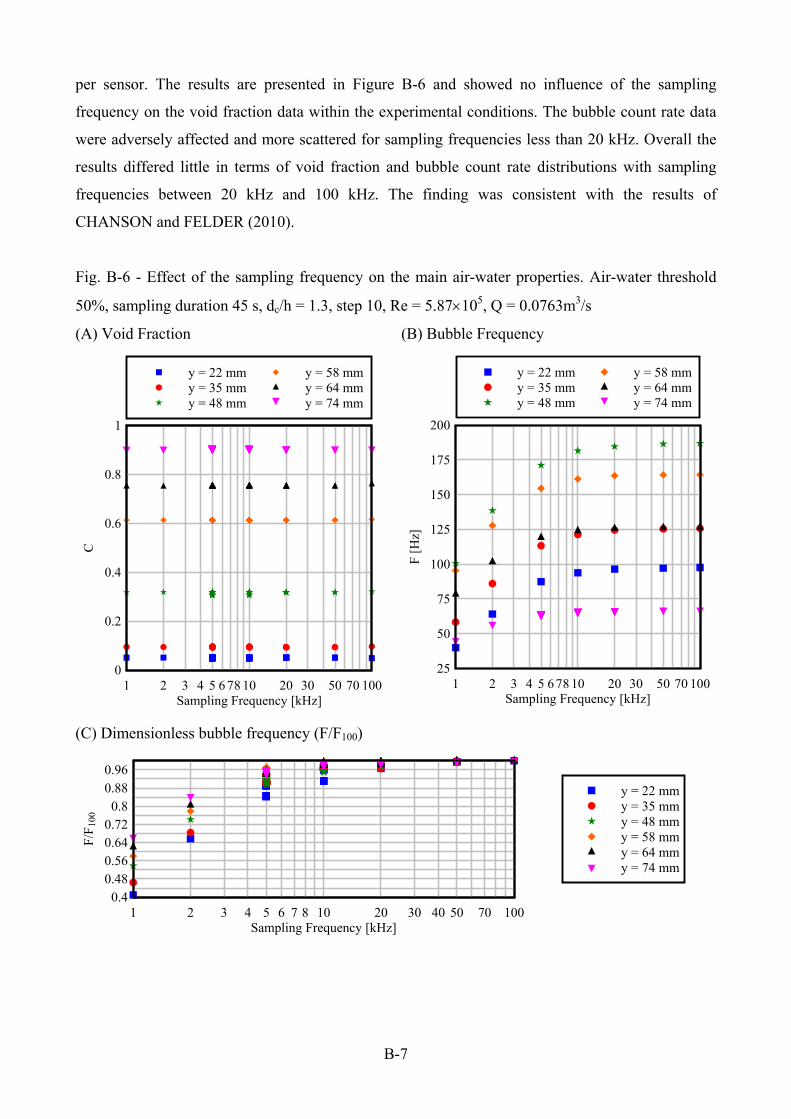
B-7
per sensor. The results are presented in Figure B-6 and showed no influence of the sampling
frequency on the void fraction data within the experimental conditions. The bubble count rate data
were adversely affected and more scattered for sampling frequencies less than 20 kHz. Overall the
results differed little in terms of void fraction and bubble count rate distributions with sampling
frequencies between 20 kHz and 100 kHz. The finding was consistent with the results of
CHANSON and FELDER (2010).
Fig. B-6 - Effect of the sampling frequency on the main air-water properties. Air-water threshold
50%, sampling duration 45 s, dc/h = 1.3, step 10, Re = 5.87105, Q = 0.0763m3/s
(A) Void Fraction (B) Bubble Frequency
Sampling Frequency [kHz]
C
1 2 3 4 5 6 78 10 20 30 50 70 1000
0.2
0.4
0.6
0.8
1
y = 22 mmy = 35 mmy = 48 mm
y = 58 mmy = 64 mmy = 74 mm
Sampling Frequency [kHz]
F [
Hz]
1 2 3 4 5 678 10 20 30 50 70 10025
50
75
100
125
150
175
200
y = 22 mmy = 35 mmy = 48 mm
y = 58 mmy = 64 mmy = 74 mm
(C) Dimensionless bubble frequency (F/F100)
Sampling Frequency [kHz]
F/F
100
1 2 3 4 5 6 7 8 10 20 30 40 50 70 1000.4
0.480.560.640.72
0.80.880.96
y = 22 mmy = 35 mmy = 48 mmy = 58 mmy = 64 mmy = 74 mm
C-1
APPENDIX C - HYDRAULIC CONDUCTIVITY TESTS
C.1 INTRODUCTION
Some experimental tests were conducted to estimate the permeability and hydraulic conductivity of
the gabions. For an one-dimensional flow through the gabions, the seepage velocity uD is given by
the Darcy law for granular non-cohesive soils:
x
HKuD
(C-1a)
where K is the hydraulic conductivity (or coefficient of permeability), H is the piezometric head and
x is the longitudinal coordinate. New experiments were conducted for a range of discharge 0.0026
m3/s < Q < 0.0129 m3/s (Table C-1). The data showed that the hydraulic conductivity was about: K
10-1 m/s (Section C.5).
Notations
A flow area (m2) perpendicular to the main stream, A = WH;
a Forchheimer flow coefficient (s/m);
b Forchheimer flow coefficient (s2/m2);
d50 characteristic size (m) of the porous medium;
g gravity constant (m/s2);
H (a) piezometric head (m);
(b) height (m) of two stacked gabion weir;
H0 height (m) of the vertical seepage face on the downstream face of the gabions;
H1 upstream head (m) above crest;
Hds water height (m) downstream of the gabion weir;
Hus water height (m) upstream of the gabion weir;
K hydraulic conductivity (m/s) of the porous medium;
Ke modified hydraulic conductivity (m/s);
L length (m) of the gabion structure in the flow direction;
L0 length (m) of the horizontal seepage face above the gabions;
Lcrest length (m) of the broad crest of the stepped facility;
Q water discharge (m3/s);
Re Reynolds number;
uD unit flux (m/s) through the pores of the gabion material, also called seepage velocity;
W channel width (m);
ΔH water height difference (m) between upstream and downstream, ΔH = Hus - Hds;
κ intrinsic permeability (m2) of the porous medium;
ν kinematic viscosity of water (m2/s).
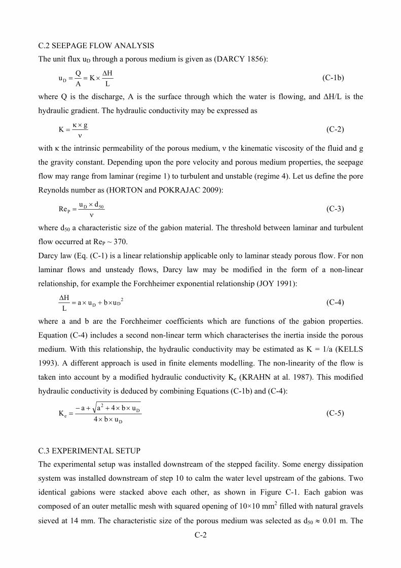
C-2
C.2 SEEPAGE FLOW ANALYSIS
The unit flux uD through a porous medium is given as (DARCY 1856):
L
HK
A
QuD
(C-1b)
where Q is the discharge, A is the surface through which the water is flowing, and ΔH/L is the
hydraulic gradient. The hydraulic conductivity may be expressed as
g
K (C-2)
with κ the intrinsic permeability of the porous medium, ν the kinematic viscosity of the fluid and g
the gravity constant. Depending upon the pore velocity and porous medium properties, the seepage
flow may range from laminar (regime 1) to turbulent and unstable (regime 4). Let us define the pore
Reynolds number as (HORTON and POKRAJAC 2009):
50DP
duRe (C-3)
where d50 a characteristic size of the gabion material. The threshold between laminar and turbulent
flow occurred at ReP ~ 370.
Darcy law (Eq. (C-1) is a linear relationship applicable only to laminar steady porous flow. For non
laminar flows and unsteady flows, Darcy law may be modified in the form of a non-linear
relationship, for example the Forchheimer exponential relationship (JOY 1991):
2DD ubua
L
H
(C-4)
where a and b are the Forchheimer coefficients which are functions of the gabion properties.
Equation (C-4) includes a second non-linear term which characterises the inertia inside the porous
medium. With this relationship, the hydraulic conductivity may be estimated as K = 1/a (KELLS
1993). A different approach is used in finite elements modelling. The non-linearity of the flow is
taken into account by a modified hydraulic conductivity Ke (KRAHN at al. 1987). This modified
hydraulic conductivity is deduced by combining Equations (C-1b) and (C-4):
D
D2
e ub4
ub4aaK
(C-5)
C.3 EXPERIMENTAL SETUP
The experimental setup was installed downstream of the stepped facility. Some energy dissipation
system was installed downstream of step 10 to calm the water level upstream of the gabions. Two
identical gabions were stacked above each other, as shown in Figure C-1. Each gabion was
composed of an outer metallic mesh with squared opening of 10×10 mm2 filled with natural gravels
sieved at 14 mm. The characteristic size of the porous medium was selected as d50 0.01 m. The
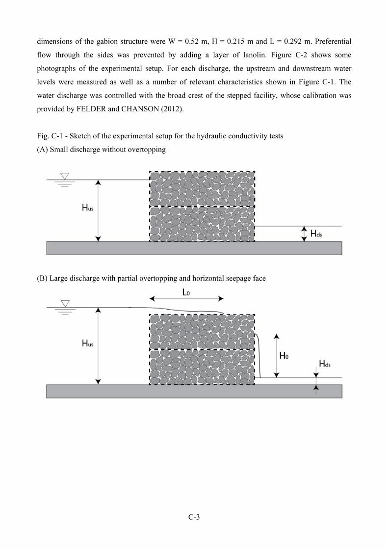
C-3
dimensions of the gabion structure were W = 0.52 m, H = 0.215 m and L = 0.292 m. Preferential
flow through the sides was prevented by adding a layer of lanolin. Figure C-2 shows some
photographs of the experimental setup. For each discharge, the upstream and downstream water
levels were measured as well as a number of relevant characteristics shown in Figure C-1. The
water discharge was controlled with the broad crest of the stepped facility, whose calibration was
provided by FELDER and CHANSON (2012).
Fig. C-1 - Sketch of the experimental setup for the hydraulic conductivity tests
(A) Small discharge without overtopping
(B) Large discharge with partial overtopping and horizontal seepage face

C-4
Fig. C-2 - Photographs of the experimental setup
(A) View from downstream (B) View from upstream
C.4 RESULTS
The results are regrouped in Table C-1. The results are presented in Figure C-3A for the linear case
(Darcy) and in Figure C-3B for the non-linear case (Forchheimer). Below, only the experiments
without overtopping were analysed.
The Darcy equation gave a hydraulic conductivity K = 1.110-1 m/s. The Forchheimer relationship
gave the following values: a = 4.31 s/m, b = 48.32 s2/m2, K = 1/a = 2.310-1 m/s. The values of the
modified hydraulic conductivity (Eq. (C.5)) are summarised in Table C-2.
Table C-1 - Values measured during the hydraulic conductivity testing for different discharges
Flow condition
Q [m3/s]
Hus [mm]
Hds [mm]
L0 [mm]
H0 [mm]
uD = Q/A[m/s]
ΔH/L [-]
Re [-]
0.0026 60.0 15.0 - - 0.023 0.154 2.3102 0.0033 85.0 19.0 - - 0.030 0.226 3.0102 0.0039 105.0 24.0 - 29.0 0.035 0.277 3.5102 0.0051 131.0 29.0 - 49.0 0.046 0.349 4.6102 0.0063 156.0 35.0 - 77.0 0.057 0.414 5.7102 0.0076 187.0 17.5 - 87.5 0.068 0.580 6.8102
Wit
hout
ov
erto
ppin
g
0.0085 210.0 20.0 - 102.0 0.076 0.651 7.6102 0.0091 218.0 23.0 45.0 105.0 0.081 0.668 8.1102 0.0098 226.0 26.0 93.0 109.0 0.087 0.685 8.7102 0.0106 232.0 28.0 140.0 125.0 0.095 0.699 9.5102 0.0114 236.0 29.0 175.0 140.0 0.102 0.709 1.0103 0.0121 240.0 30.0 215.0 175.0 0.108 0.719 1.1103
Wit
h ov
erto
ppin
g
0.0129 242.0 30.0 245.0 180.0 0.115 0.726 1.2103
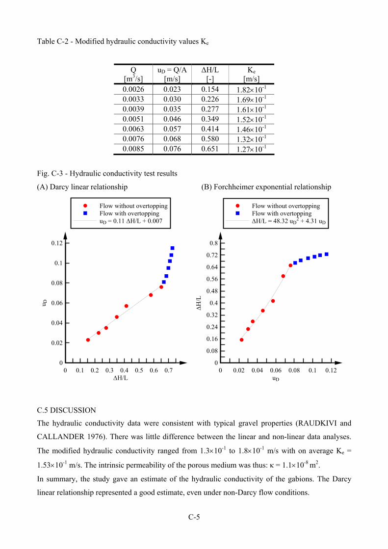
C-5
Table C-2 - Modified hydraulic conductivity values Ke
Q [m3/s]
uD = Q/A [m/s]
ΔH/L [-]
Ke
[m/s] 0.0026 0.023 0.154 1.8210-1 0.0033 0.030 0.226 1.6910-1 0.0039 0.035 0.277 1.6110-1 0.0051 0.046 0.349 1.5210-1 0.0063 0.057 0.414 1.4610-1 0.0076 0.068 0.580 1.3210-1 0.0085 0.076 0.651 1.2710-1
Fig. C-3 - Hydraulic conductivity test results
(A) Darcy linear relationship (B) Forchheimer exponential relationship
H/L
u D
0 0.1 0.2 0.3 0.4 0.5 0.6 0.70
0.02
0.04
0.06
0.08
0.1
0.12
Flow without overtoppingFlow with overtoppinguD = 0.11 H/L + 0.007
uD
H
/L
0 0.02 0.04 0.06 0.08 0.1 0.120
0.08
0.16
0.24
0.32
0.4
0.48
0.56
0.64
0.72
0.8
Flow without overtoppingFlow with overtoppingH/L = 48.32 uD
2 + 4.31 uD
C.5 DISCUSSION
The hydraulic conductivity data were consistent with typical gravel properties (RAUDKIVI and
CALLANDER 1976). There was little difference between the linear and non-linear data analyses.
The modified hydraulic conductivity ranged from 1.310-1 to 1.810-1 m/s with on average Ke =
1.5310-1 m/s. The intrinsic permeability of the porous medium was thus: κ = 1.110-8 m2.
In summary, the study gave an estimate of the hydraulic conductivity of the gabions. The Darcy
linear relationship represented a good estimate, even under non-Darcy flow conditions.
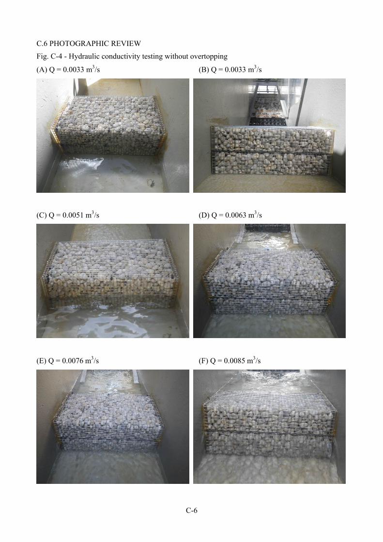
C-6
C.6 PHOTOGRAPHIC REVIEW
Fig. C-4 - Hydraulic conductivity testing without overtopping
(A) Q = 0.0033 m3/s (B) Q = 0.0033 m3/s
(C) Q = 0.0051 m3/s (D) Q = 0.0063 m3/s
(E) Q = 0.0076 m3/s (F) Q = 0.0085 m3/s
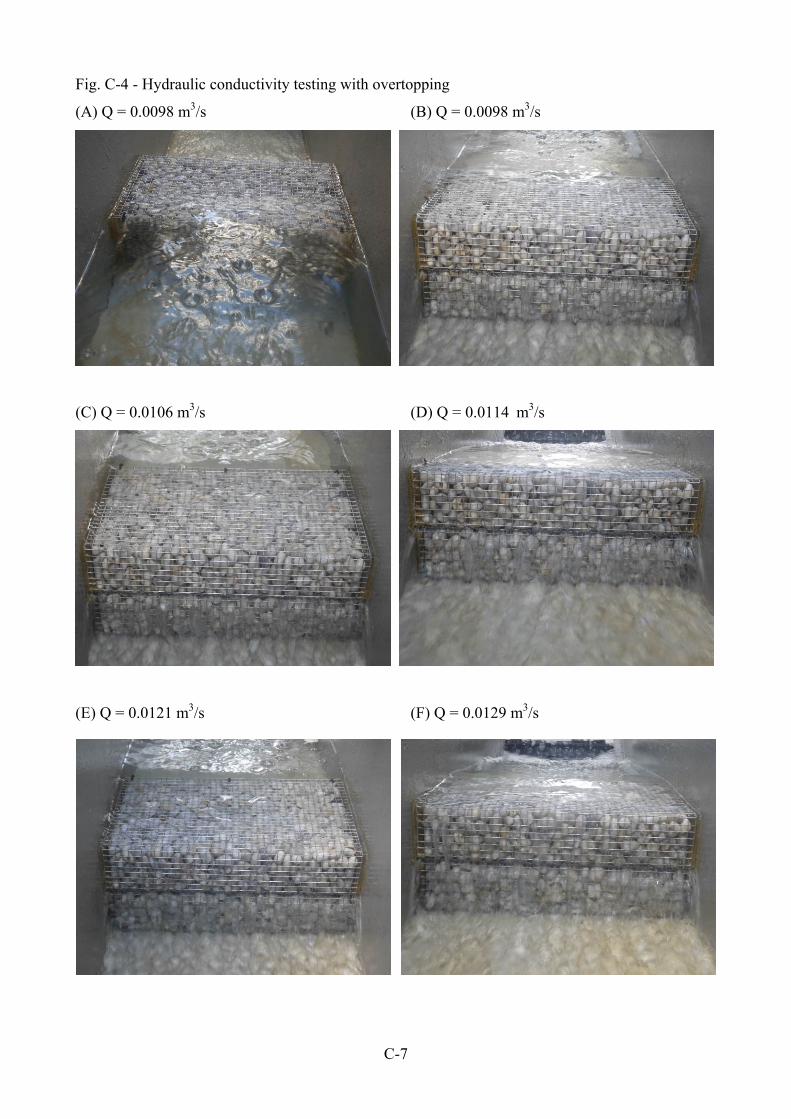
C-7
Fig. C-4 - Hydraulic conductivity testing with overtopping
(A) Q = 0.0098 m3/s (B) Q = 0.0098 m3/s
(C) Q = 0.0106 m3/s (D) Q = 0.0114 m3/s
(E) Q = 0.0121 m3/s (F) Q = 0.0129 m3/s
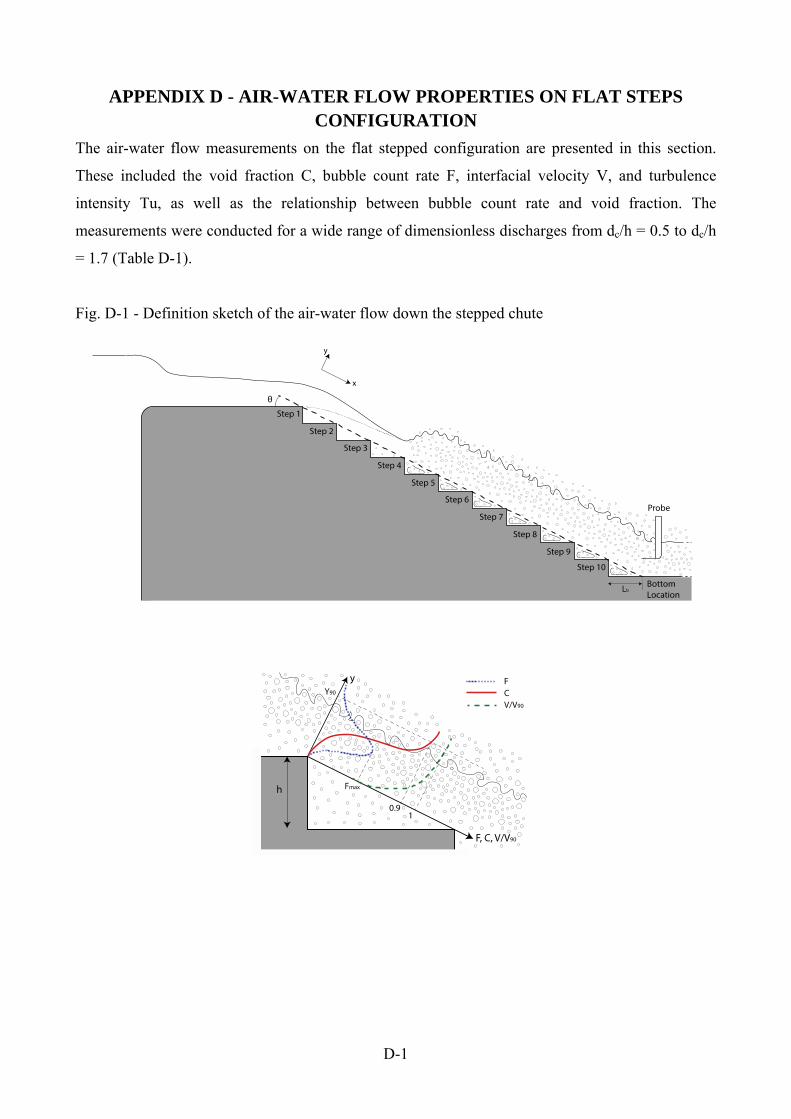
D-1
APPENDIX D - AIR-WATER FLOW PROPERTIES ON FLAT STEPS CONFIGURATION
The air-water flow measurements on the flat stepped configuration are presented in this section.
These included the void fraction C, bubble count rate F, interfacial velocity V, and turbulence
intensity Tu, as well as the relationship between bubble count rate and void fraction. The
measurements were conducted for a wide range of dimensionless discharges from dc/h = 0.5 to dc/h
= 1.7 (Table D-1).
Fig. D-1 - Definition sketch of the air-water flow down the stepped chute
D-2
Notation
C void fraction defined as the volume of air per unit volume;
Cmean depth averaged void fraction defined in terms of Y90: Cmean = 1 - d/Y90;
dc critical flow depth (m);
F bubble count rate (Hz) defined as the number of detected air bubbles per unit time;
Fmax maximum bubble count rate (Hz) in a cross-section;
h vertical step height (m);
Q water discharge (m3/s);
qw water discharge per unit width calculated from the integration of the measured void
fraction and velocity profiles:
90Y
0
w dyVC1q
Re Reynolds number defined in terms of hydraulic diameter;
Tu turbulence intensity;
Tumax maximum turbulence intensity in a cross section;
V interfacial velocity (m/s);
V90 interfacial velocity (m/s) at y = Y90;
y distance (m) perpendicular to the pseudo-bottom bottom formed by the step edges;
Y90 characteristic distance (m) where the void fraction equals 0.90;
Δx streamwise distance (m) between probe tips;
Δz transversal distance (m) between probe tips;
Ø diameter (m) of inner probe sensor;
θ chute slope;
Abbreviations
NA nappe flow regime;
TRA transition flow regime;
SK skimming flow regime.

D-3
Fig. D-2 - Air-water flow properties on the flat stepped spillway (θ = 26.6°) as functions of y/dc -
NA: dc/h = 0.5, Q = 0.018 m3/s, Re = 1.40×10⁵; step edges 3-10. Legend applies to all figures.
(A) Void fraction distribution (B) Bubble count rate distribution
C
y / d
c
0 0.1 0.2 0.3 0.4 0.5 0.6 0.7 0.8 0.9 10
0.25
0.5
0.75
1
1.25
1.5
1.75
2
2.25
2.5
F x dc / Vc
y / d
c
0 2 4 6 8 10 12 140
0.25
0.5
0.75
1
1.25
1.5
1.75
2
2.25
2.5
(C) Velocity distribution (D) Turbulent intensity distribution
V / Vc
y / d
c
0 0.75 1.5 2.25 3 3.75 4.50
0.25
0.5
0.75
1
1.25
1.5
1.75
2
2.25
2.5
Tu
y / d
c
0 0.4 0.8 1.2 1.6 2 2.4 2.8 3.2 3.60
0.25
0.5
0.75
1
1.25
1.5
1.75
2
2.25
2.5
(E) Relationship between bubble count rate and void fraction
C
F x
dc
/ Vc
0 0.1 0.2 0.3 0.4 0.5 0.6 0.7 0.8 0.9 10
2
4
6
8
10
12
14
Step edge 3Step edge 4Step edge 5Step edge 6Step edge 7Step edge 8Step edge 9Step edge 10
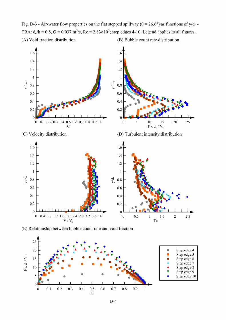
D-4
Fig. D-3 - Air-water flow properties on the flat stepped spillway (θ = 26.6°) as functions of y/dc -
TRA: dc/h = 0.8, Q = 0.037 m3/s, Re = 2.83×10⁵; step edges 4-10. Legend applies to all figures.
(A) Void fraction distribution (B) Bubble count rate distribution
C
y / d
c
0 0.1 0.2 0.3 0.4 0.5 0.6 0.7 0.8 0.9 10
0.2
0.4
0.6
0.8
1
1.2
1.4
1.6
F x dc / Vc
y / d
c
0 5 10 15 20 250
0.2
0.4
0.6
0.8
1
1.2
1.4
1.6
(C) Velocity distribution (D) Turbulent intensity distribution
V / Vc
y / d
c
0 0.4 0.8 1.2 1.6 2 2.4 2.8 3.2 3.6 40
0.2
0.4
0.6
0.8
1
1.2
1.4
1.6
Tu
y/dc
0 0.5 1 1.5 2 2.50
0.2
0.4
0.6
0.8
1
1.2
1.4
1.6
(E) Relationship between bubble count rate and void fraction
C
F x
dc
/ Vc
0 0.1 0.2 0.3 0.4 0.5 0.6 0.7 0.8 0.9 10
5
10
15
20
25
Step edge 4Step edge 5Step edge 6Step edge 7Step edge 8Step edge 9Step edge 10
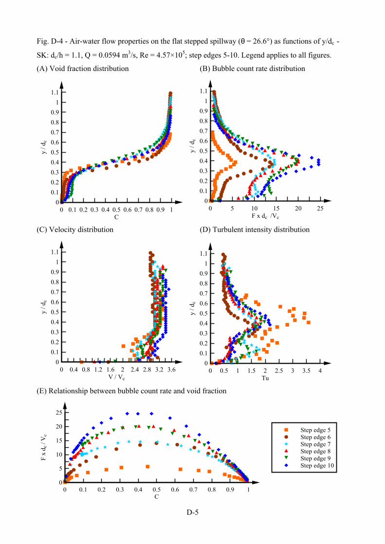
D-5
Fig. D-4 - Air-water flow properties on the flat stepped spillway (θ = 26.6°) as functions of y/dc -
SK: dc/h = 1.1, Q = 0.0594 m3/s, Re = 4.57×10⁵; step edges 5-10. Legend applies to all figures.
(A) Void fraction distribution (B) Bubble count rate distribution
C
y / d
c
0 0.1 0.2 0.3 0.4 0.5 0.6 0.7 0.8 0.9 10
0.1
0.2
0.3
0.4
0.5
0.6
0.7
0.8
0.9
1
1.1
F x dc /Vc
y / d
c
0 5 10 15 20 250
0.1
0.2
0.3
0.4
0.5
0.6
0.7
0.8
0.9
1
1.1
(C) Velocity distribution (D) Turbulent intensity distribution
V / Vc
y / d
c
0 0.4 0.8 1.2 1.6 2 2.4 2.8 3.2 3.60
0.1
0.2
0.3
0.4
0.5
0.6
0.7
0.8
0.9
1
1.1
Tu
y / d
c
0 0.5 1 1.5 2 2.5 3 3.5 40
0.1
0.2
0.3
0.4
0.5
0.6
0.7
0.8
0.9
1
1.1
(E) Relationship between bubble count rate and void fraction
C
F x
dc
/ Vc
0 0.1 0.2 0.3 0.4 0.5 0.6 0.7 0.8 0.9 10
5
10
15
20
25
Step edge 5Step edge 6Step edge 7Step edge 8Step edge 9Step edge 10
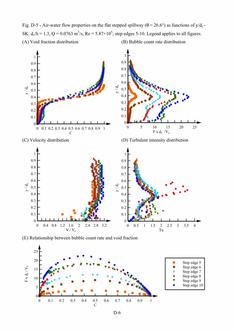
D-6
Fig. D-5 - Air-water flow properties on the flat stepped spillway (θ = 26.6°) as functions of y/dc -
SK: dc/h = 1.3, Q = 0.0763 m3/s, Re = 5.87×10⁵; step edges 5-10. Legend applies to all figures.
(A) Void fraction distribution (B) Bubble count rate distribution
C
y / d
c
0 0.1 0.2 0.3 0.4 0.5 0.6 0.7 0.8 0.9 10
0.1
0.2
0.3
0.4
0.5
0.6
0.7
0.8
0.9
1
F x dc /Vc
y / d
c
0 5 10 15 20 250
0.1
0.2
0.3
0.4
0.5
0.6
0.7
0.8
0.9
1
(C) Velocity distribution (D) Turbulent intensity distribution
V / Vc
y / d
c
0 0.4 0.8 1.2 1.6 2 2.4 2.8 3.20
0.1
0.2
0.3
0.4
0.5
0.6
0.7
0.8
0.9
1
Tu
y / d
c
0 0.5 1 1.5 2 2.5 3 3.5 40
0.1
0.2
0.3
0.4
0.5
0.6
0.7
0.8
0.9
1
(E) Relationship between bubble count rate and void fraction
C
F x
dc
/ Vc
0 0.1 0.2 0.3 0.4 0.5 0.6 0.7 0.8 0.9 10
5
10
15
20
25
Step edge 5Step edge 6Step edge 7Step edge 8Step edge 9Step edge 10
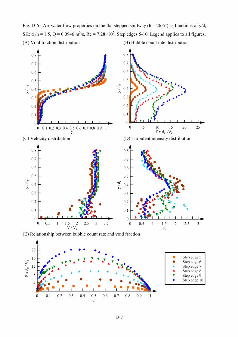
D-7
Fig. D-6 - Air-water flow properties on the flat stepped spillway (θ = 26.6°) as functions of y/dc -
SK: dc/h = 1.5, Q = 0.0946 m3/s, Re = 7.28×10⁵; Step edges 5-10. Legend applies to all figures.
(A) Void fraction distribution (B) Bubble count rate distribution
C
y / d
c
0 0.1 0.2 0.3 0.4 0.5 0.6 0.7 0.8 0.9 10
0.1
0.2
0.3
0.4
0.5
0.6
0.7
0.8
F x dc /Vc
y / d
c
0 5 10 15 20 250
0.1
0.2
0.3
0.4
0.5
0.6
0.7
0.8
(C) Velocity distribution (D) Turbulent intensity distribution
V / Vc
y / d
c
0 0.5 1 1.5 2 2.5 3 3.50
0.1
0.2
0.3
0.4
0.5
0.6
0.7
0.8
Tu
y / d
c
0 0.5 1 1.5 2 2.5 30
0.1
0.2
0.3
0.4
0.5
0.6
0.7
0.8
(E) Relationship between bubble count rate and void fraction
C
F x
dc
/ Vc
0 0.1 0.2 0.3 0.4 0.5 0.6 0.7 0.8 0.9 10
4
8
12
16
20
Step edge 5Step edge 6Step edge 7Step edge 8Step edge 9Step edge 10

D-8
Fig. D-7 - Air-water flow properties on the flat stepped spillway (θ = 26.6°) as functions of y/dc -
SK: dc/h = 1.7, Q = 0.114 m3/s, Re = 8.78×10⁵; Step edges 6-10. Legend applies to all figures.
(A) Void fraction distribution (B) Bubble count rate distribution
C
y / d
c
0 0.1 0.2 0.3 0.4 0.5 0.6 0.7 0.8 0.9 10
0.1
0.2
0.3
0.4
0.5
0.6
0.7
0.8
F x dc /Vc
y / d
c
0 2 4 6 8 10 12 14 16 180
0.1
0.2
0.3
0.4
0.5
0.6
0.7
0.8
(C) Velocity distribution (D) Turbulent intensity distribution
V / Vc
y / d
c
0 0.5 1 1.5 2 2.5 3 3.50
0.1
0.2
0.3
0.4
0.5
0.6
0.7
0.8
Tu
y / d
c
0 0.5 1 1.5 2 2.50
0.1
0.2
0.3
0.4
0.5
0.6
0.7
0.8
(E) Relationship between bubble count rate and void fraction
C
F x
dc
/ Vc
0 0.1 0.2 0.3 0.4 0.5 0.6 0.7 0.8 0.9 102468
1012141618
Step edge 6Step edge 7Step edge 8Step edge 9Step edge 10
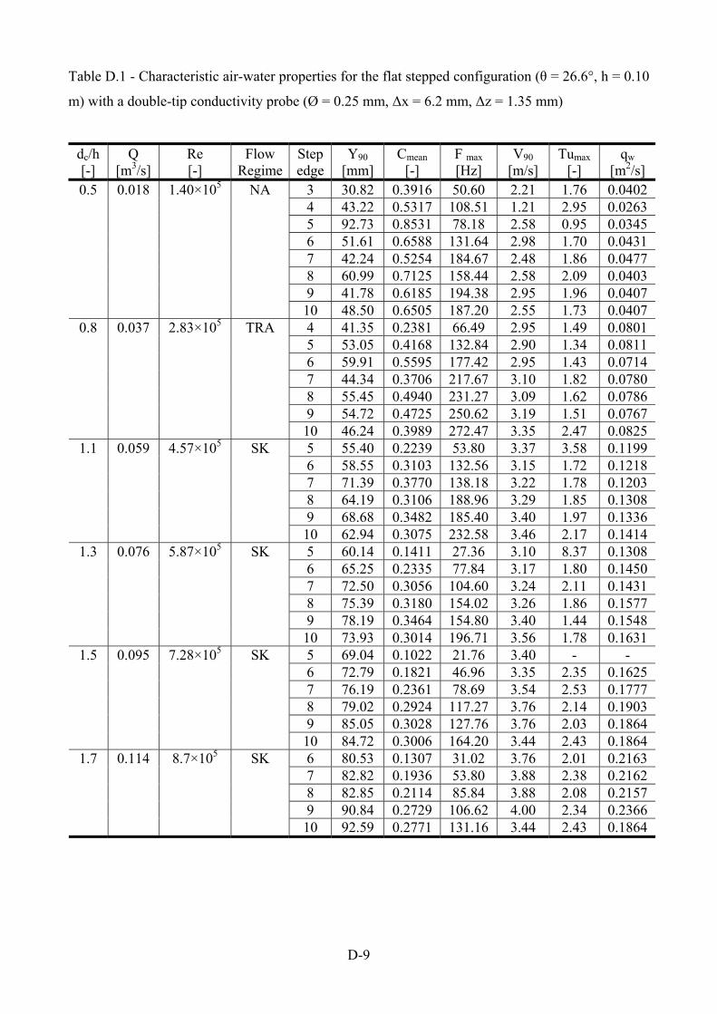
D-9
Table D.1 - Characteristic air-water properties for the flat stepped configuration (θ = 26.6°, h = 0.10
m) with a double-tip conductivity probe (Ø = 0.25 mm, Δx = 6.2 mm, Δz = 1.35 mm)
dc/h [-]
Q [m3/s]
Re [-]
Flow Regime
Step edge
Y90 [mm]
Cmean [-]
F max
[Hz] V90
[m/s] Tumax
[-] qw
[m2/s] 3 30.82 0.3916 50.60 2.21 1.76 0.0402 4 43.22 0.5317 108.51 1.21 2.95 0.0263 5 92.73 0.8531 78.18 2.58 0.95 0.0345 6 51.61 0.6588 131.64 2.98 1.70 0.0431 7 42.24 0.5254 184.67 2.48 1.86 0.0477 8 60.99 0.7125 158.44 2.58 2.09 0.0403 9 41.78 0.6185 194.38 2.95 1.96 0.0407
0.5 0.018 1.40×10⁵ NA
10 48.50 0.6505 187.20 2.55 1.73 0.0407 4 41.35 0.2381 66.49 2.95 1.49 0.0801 5 53.05 0.4168 132.84 2.90 1.34 0.0811 6 59.91 0.5595 177.42 2.95 1.43 0.0714 7 44.34 0.3706 217.67 3.10 1.82 0.0780 8 55.45 0.4940 231.27 3.09 1.62 0.0786 9 54.72 0.4725 250.62 3.19 1.51 0.0767
0.8 0.037 2.83×10⁵ TRA
10 46.24 0.3989 272.47 3.35 2.47 0.0825 5 55.40 0.2239 53.80 3.37 3.58 0.1199 6 58.55 0.3103 132.56 3.15 1.72 0.1218 7 71.39 0.3770 138.18 3.22 1.78 0.1203 8 64.19 0.3106 188.96 3.29 1.85 0.1308 9 68.68 0.3482 185.40 3.40 1.97 0.1336
1.1 0.059 4.57×10⁵ SK
10 62.94 0.3075 232.58 3.46 2.17 0.1414 5 60.14 0.1411 27.36 3.10 8.37 0.1308 6 65.25 0.2335 77.84 3.17 1.80 0.1450 7 72.50 0.3056 104.60 3.24 2.11 0.1431 8 75.39 0.3180 154.02 3.26 1.86 0.1577 9 78.19 0.3464 154.80 3.40 1.44 0.1548
1.3 0.076 5.87×10⁵ SK
10 73.93 0.3014 196.71 3.56 1.78 0.1631 5 69.04 0.1022 21.76 3.40 - - 6 72.79 0.1821 46.96 3.35 2.35 0.1625 7 76.19 0.2361 78.69 3.54 2.53 0.1777 8 79.02 0.2924 117.27 3.76 2.14 0.1903 9 85.05 0.3028 127.76 3.76 2.03 0.1864
1.5 0.095 7.28×10⁵ SK
10 84.72 0.3006 164.20 3.44 2.43 0.1864 6 80.53 0.1307 31.02 3.76 2.01 0.2163 7 82.82 0.1936 53.80 3.88 2.38 0.2162 8 82.85 0.2114 85.84 3.88 2.08 0.2157 9 90.84 0.2729 106.62 4.00 2.34 0.2366
1.7 0.114 8.7×10⁵ SK
10 92.59 0.2771 131.16 3.44 2.43 0.1864
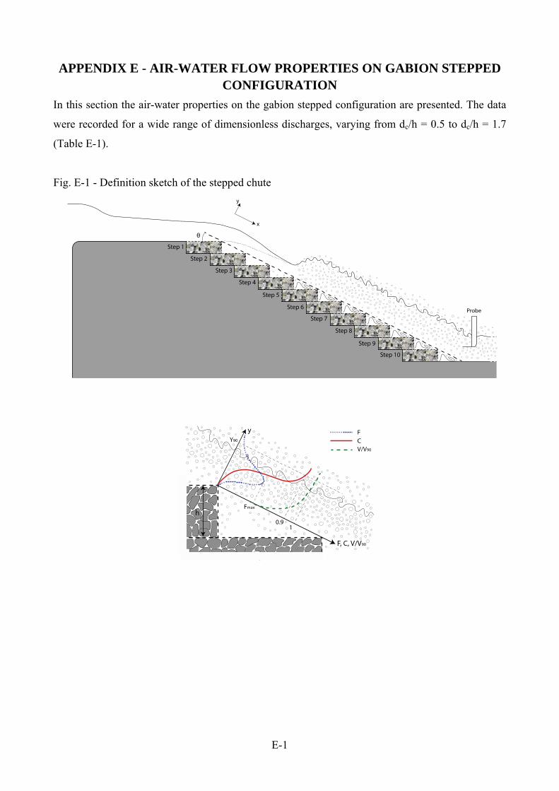
E-1
APPENDIX E - AIR-WATER FLOW PROPERTIES ON GABION STEPPED CONFIGURATION
In this section the air-water properties on the gabion stepped configuration are presented. The data
were recorded for a wide range of dimensionless discharges, varying from dc/h = 0.5 to dc/h = 1.7
(Table E-1).
Fig. E-1 - Definition sketch of the stepped chute

E-2
Notation
C void fraction defined as the volume of air per unit volume;
Cmean depth averaged void fraction defined in terms of Y90: Cmean = 1 - d/Y90;
dc critical flow depth (m);
F bubble count rate (Hz) defined as the number of detected air bubbles per unit time;
Fmax maximum bubble count rate (Hz) in a cross-section;
h vertical step height (m);
Q water discharge (m3/s);
qw water discharge per unit width calculated from the integration of the measured void
fraction and velocity profiles:
90Y
0
w dyVC1q
Re Reynolds number defined in terms of hydraulic diameter;
Tu turbulence intensity;
Tumax maximum turbulence intensity in a cross section;
V interfacial velocity (m/s);
V90 interfacial velocity (m/s) at y = Y90;
y distance (m) perpendicular to the pseudo-bottom bottom formed by the step edges;
Y90 characteristic distance (m) where the void fraction equals 0.90;
Δx streamwise distance (m) between probe tips;
Δz transversal distance (m) between probe tips;
Ø diameter (m) of inner probe sensor;
θ chute slope;
Abbreviations
NA nappe flow regime;
TRA transition flow regime;
SK skimming flow regime.
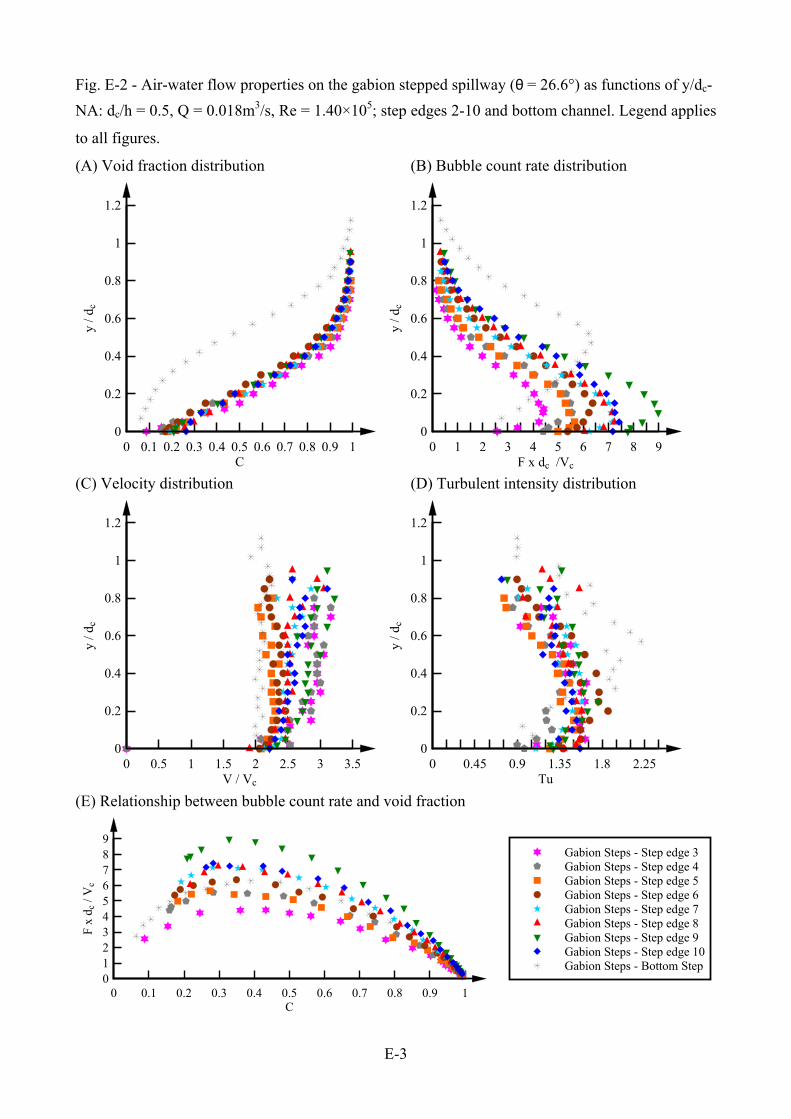
E-3
Fig. E-2 - Air-water flow properties on the gabion stepped spillway (θ = 26.6°) as functions of y/dc-
NA: dc/h = 0.5, Q = 0.018m3/s, Re = 1.40×10⁵; step edges 2-10 and bottom channel. Legend applies
to all figures.
(A) Void fraction distribution (B) Bubble count rate distribution
C
y / d
c
0 0.1 0.2 0.3 0.4 0.5 0.6 0.7 0.8 0.9 10
0.2
0.4
0.6
0.8
1
1.2
F x dc /Vc
y / d
c
0 1 2 3 4 5 6 7 8 90
0.2
0.4
0.6
0.8
1
1.2
(C) Velocity distribution (D) Turbulent intensity distribution
V / Vc
y / d
c
0 0.5 1 1.5 2 2.5 3 3.50
0.2
0.4
0.6
0.8
1
1.2
Tu
y / d
c
0 0.45 0.9 1.35 1.8 2.250
0.2
0.4
0.6
0.8
1
1.2
(E) Relationship between bubble count rate and void fraction
C
F x
dc
/ Vc
0 0.1 0.2 0.3 0.4 0.5 0.6 0.7 0.8 0.9 10123456789
Gabion Steps - Step edge 3Gabion Steps - Step edge 4Gabion Steps - Step edge 5Gabion Steps - Step edge 6Gabion Steps - Step edge 7Gabion Steps - Step edge 8Gabion Steps - Step edge 9Gabion Steps - Step edge 10Gabion Steps - Bottom Step

E-4
Fig. E-3 - Air-water flow properties on the gabion stepped spillway (θ = 26.6°) as functions of y/dc-
TRA: dc/h = 0.8, Q = 0.036m3/s, Re = 2.83×10⁵; step edges 4-10and bottom channel. Legend
applies to all figures.
(A) Void fraction distribution (B) Bubble count rate distribution
C
y / d
c
0 0.1 0.2 0.3 0.4 0.5 0.6 0.7 0.8 0.9 10
0.2
0.4
0.6
0.8
1
1.2
F x dc /Vc
y / d
c
0 5 10 15 20 250
0.2
0.4
0.6
0.8
1
1.2
(C) Velocity distribution (D) Turbulent intensity distribution
V / Vc
y / d
c
0 0.4 0.8 1.2 1.6 2 2.4 2.8 3.2 3.60
0.2
0.4
0.6
0.8
1
1.2
Tu
y / d
c
0 0.5 1 1.5 2 2.50
0.2
0.4
0.6
0.8
1
1.2
(E) Relationship between bubble count rate and void fraction
C
F x
dc
/ Vc
0 0.1 0.2 0.3 0.4 0.5 0.6 0.7 0.8 0.9 10
5
10
15
20
25
Gabion steps - Step edge 4Gabion steps - Step edge 5Gabion steps - Step edge 6Gabion steps - Step edge 7Gabion steps - Step edge 8Gabion steps - Step edge 9Gabion steps - Step edge 10Gabion steps - Bottom Step
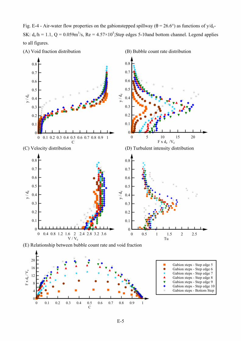
E-5
Fig. E-4 - Air-water flow properties on the gabionstepped spillway (θ = 26.6°) as functions of y/dc-
SK: dc/h = 1.1, Q = 0.059m3/s, Re = 4.57×10⁵;Step edges 5-10and bottom channel. Legend applies
to all figures.
(A) Void fraction distribution (B) Bubble count rate distribution
C
y / d
c
0 0.1 0.2 0.3 0.4 0.5 0.6 0.7 0.8 0.9 10
0.1
0.2
0.3
0.4
0.5
0.6
0.7
0.8
F x dc /Vc
y / d
c
0 5 10 15 200
0.1
0.2
0.3
0.4
0.5
0.6
0.7
0.8
(C) Velocity distribution (D) Turbulent intensity distribution
V / Vc
y / d
c
0 0.4 0.8 1.2 1.6 2 2.4 2.8 3.2 3.60
0.1
0.2
0.3
0.4
0.5
0.6
0.7
0.8
Tu
y / d
c
0 0.5 1 1.5 2 2.50
0.1
0.2
0.3
0.4
0.5
0.6
0.7
0.8
(E) Relationship between bubble count rate and void fraction
C
F x
dc
/ Vc
0 0.1 0.2 0.3 0.4 0.5 0.6 0.7 0.8 0.9 10
4
8
12
16
20Gabion steps - Step edge 5Gabion steps - Step edge 6Gabion steps - Step edge 7Gabion steps - Step edge 8Gabion steps - Step edge 9Gabion steps - Step edge 10Gabion steps - Bottom Step

E-6
Fig. E-5 - Air-water flow properties on the gabionstepped spillway (θ = 26.6°) as functions of y/dc -
SK: dc/h = 1.3, Q = 0.076m3/s, Re = 5.87×10⁵; Step edges 6-10and bottom channel. Legend applies
to all figures.
(A) Void fraction distribution (B) Bubble count rate distribution
C
y / d
c
0 0.1 0.2 0.3 0.4 0.5 0.6 0.7 0.8 0.9 10
0.1
0.2
0.3
0.4
0.5
0.6
0.7
0.8
F x dc /Vc
y / d
c
0 2 4 6 8 10 12 14 16 18 200
0.1
0.2
0.3
0.4
0.5
0.6
0.7
0.8
(C) Velocity distribution (D) Turbulent intensity distribution
V / Vc
y / d
c
0 0.4 0.8 1.2 1.6 2 2.4 2.8 3.2 3.60
0.1
0.2
0.3
0.4
0.5
0.6
0.7
0.8
Tu
y / d
c
0 0.5 1 1.5 2 2.50
0.1
0.2
0.3
0.4
0.5
0.6
0.7
0.8
(E) Relationship between bubble count rate and void fraction
C
y / d
c
0 0.1 0.2 0.3 0.4 0.5 0.6 0.7 0.8 0.9 10
3
6
9
12
15
18
Gabion steps - Step edge 6Gabion steps - Step edge 7Gabion steps - Step edge 8Gabion steps - Step edge 9Gabion steps - Step edge 10Gabion steps - Bottom Step

E-7
Fig. E-6 - Air-water flow properties on the gabionstepped spillway (θ = 26.6°) as functions of y/dc-
SK: dc/h = 1.5, Q = 0.094m3/s, Re = 7.28×10⁵; Step edges 8-10 and bottom step. Legend applies to
all figures.
(A) Void fraction distribution (B) Bubble count rate distribution
C
y / d
c
0 0.1 0.2 0.3 0.4 0.5 0.6 0.7 0.8 0.9 10
0.1
0.2
0.3
0.4
0.5
0.6
0.7
F x dc / Vc
y / d
c
0 2 4 6 8 10 12 14 16 180
0.1
0.2
0.3
0.4
0.5
0.6
0.7
(C) Velocity distribution (D) Turbulent intensity distribution
V / Vc
y / d
c
0 0.5 1 1.5 2 2.5 3 3.50
0.1
0.2
0.3
0.4
0.5
0.6
0.7
Tu
y / d
c
0 0.5 1 1.5 2 2.50
0.1
0.2
0.3
0.4
0.5
0.6
0.7
(E) Relationship between bubble count rate and void fraction
C
F x
dc
/ Vc
0 0.1 0.2 0.3 0.4 0.5 0.6 0.7 0.8 0.9 102468
1012141618
Gabion steps - Step edge 8Gabion steps - Step edge 9Gabion steps - Step edge 10Gabion steps - Bottom Step

E-8
Fig. E-7 - Air-water flow properties on the gabionstepped spillway (θ = 26.6°) as functions of y/dc-
SK: dc/h = 1.7, Q = 0.114m3/s, Re = 8.78×10⁵; step edges 8-10 and bottom step. Legend applies to
all figures.
(A) Void fraction distribution (B) Bubble count rate distribution
C
y / d
c
0 0.1 0.2 0.3 0.4 0.5 0.6 0.7 0.8 0.9 10
0.1
0.2
0.3
0.4
0.5
0.6
0.7
F x dc /Vc
y / d
c
0 2 4 6 8 10 12 140
0.1
0.2
0.3
0.4
0.5
0.6
0.7
(C) Velocity distribution (D) Turbulent intensity distribution
V / Vc
y / d
c
0 0.5 1 1.5 2 2.5 3 3.50
0.1
0.2
0.3
0.4
0.5
0.6
0.7
Tu
y / d
c
0 0.5 1 1.5 2 2.50
0.1
0.2
0.3
0.4
0.5
0.6
0.7
(E) Relationship between bubble count rate and void fraction
C
F x
dc
/ Vc
0 0.1 0.2 0.3 0.4 0.5 0.6 0.7 0.8 0.9 10
2
4
6
8
10
12
14
Gabion steps - Step edge 8Gabion steps - Step edge 9Gabion steps - Step edge 10Gabion steps - Bottom Step
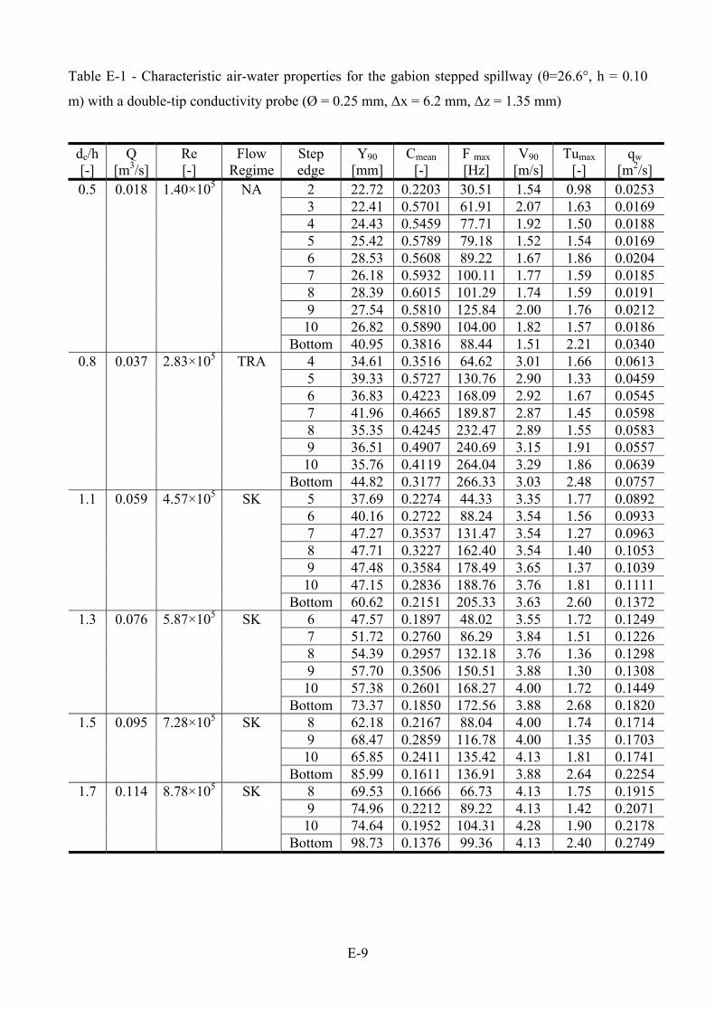
E-9
Table E-1 - Characteristic air-water properties for the gabion stepped spillway (θ=26.6°, h = 0.10
m) with a double-tip conductivity probe (Ø = 0.25 mm, Δx = 6.2 mm, Δz = 1.35 mm)
dc/h [-]
Q [m3/s]
Re [-]
Flow Regime
Step edge
Y90 [mm]
Cmean [-]
F max
[Hz] V90
[m/s] Tumax
[-] qw
[m2/s] 2 22.72 0.2203 30.51 1.54 0.98 0.0253 3 22.41 0.5701 61.91 2.07 1.63 0.0169 4 24.43 0.5459 77.71 1.92 1.50 0.0188 5 25.42 0.5789 79.18 1.52 1.54 0.0169 6 28.53 0.5608 89.22 1.67 1.86 0.0204 7 26.18 0.5932 100.11 1.77 1.59 0.0185 8 28.39 0.6015 101.29 1.74 1.59 0.0191 9 27.54 0.5810 125.84 2.00 1.76 0.0212 10 26.82 0.5890 104.00 1.82 1.57 0.0186
0.5 0.018 1.40×10⁵ NA
Bottom 40.95 0.3816 88.44 1.51 2.21 0.0340 4 34.61 0.3516 64.62 3.01 1.66 0.0613 5 39.33 0.5727 130.76 2.90 1.33 0.0459 6 36.83 0.4223 168.09 2.92 1.67 0.0545 7 41.96 0.4665 189.87 2.87 1.45 0.0598 8 35.35 0.4245 232.47 2.89 1.55 0.0583 9 36.51 0.4907 240.69 3.15 1.91 0.0557 10 35.76 0.4119 264.04 3.29 1.86 0.0639
0.8 0.037 2.83×10⁵ TRA
Bottom 44.82 0.3177 266.33 3.03 2.48 0.0757 5 37.69 0.2274 44.33 3.35 1.77 0.0892 6 40.16 0.2722 88.24 3.54 1.56 0.0933 7 47.27 0.3537 131.47 3.54 1.27 0.0963 8 47.71 0.3227 162.40 3.54 1.40 0.1053 9 47.48 0.3584 178.49 3.65 1.37 0.1039 10 47.15 0.2836 188.76 3.76 1.81 0.1111
1.1 0.059 4.57×10⁵ SK
Bottom 60.62 0.2151 205.33 3.63 2.60 0.1372 6 47.57 0.1897 48.02 3.55 1.72 0.1249 7 51.72 0.2760 86.29 3.84 1.51 0.1226 8 54.39 0.2957 132.18 3.76 1.36 0.1298 9 57.70 0.3506 150.51 3.88 1.30 0.1308 10 57.38 0.2601 168.27 4.00 1.72 0.1449
1.3 0.076 5.87×10⁵ SK
Bottom 73.37 0.1850 172.56 3.88 2.68 0.1820 8 62.18 0.2167 88.04 4.00 1.74 0.1714 9 68.47 0.2859 116.78 4.00 1.35 0.1703 10 65.85 0.2411 135.42 4.13 1.81 0.1741
1.5 0.095 7.28×10⁵ SK
Bottom 85.99 0.1611 136.91 3.88 2.64 0.2254 8 69.53 0.1666 66.73 4.13 1.75 0.1915 9 74.96 0.2212 89.22 4.13 1.42 0.2071 10 74.64 0.1952 104.31 4.28 1.90 0.2178
1.7 0.114 8.78×10⁵ SK
Bottom 98.73 0.1376 99.36 4.13 2.40 0.2749

F-1
APPENDIX F - AIR-WATER FLOW PROPERTIES ON CAPPED STEPPED CONFIGURATION
In this section the air-water properties measured on the capped stepped configuration are presented.
The basic air-water properties include the void fraction (C), the Bubble count rate (F), the
interfacial velocity (V), the turbulent intensity (Tu) and the relationship between the Bubble count
rate and the void fraction. The distributions were recorded for a wide range of dimensionless
discharges, varying from dc/h = 0.5 to dc/h = 1.7 (Table F.1). The characteristic air-water properties
are summarised in dimensioned form in Table F.1.
Fig. F-1 - Definition sketch of the stepped chute

F-2
Notation
C void fraction defined as the volume of air per unit volume;
Cmean depth averaged void fraction defined in terms of Y90: Cmean = 1 - d/Y90;
dc critical flow depth (m);
F bubble count rate (Hz) defined as the number of detected air bubbles per unit time;
Fmax maximum bubble count rate (Hz) in a cross-section;
h vertical step height (m);
Q water discharge (m3/s);
qw water discharge per unit width calculated from the integration of the measured void
fraction and velocity profiles:
90Y
0
w dyVC1q
Re Reynolds number defined in terms of hydraulic diameter;
Tu turbulence intensity;
Tumax maximum turbulence intensity in a cross section;
V interfacial velocity (m/s);
V90 interfacial velocity (m/s) at y = Y90;
y distance (m) perpendicular to the pseudo-bottom bottom formed by the step edges;
Y90 characteristic distance (m) where the void fraction equals 0.90;
Δx streamwise distance (m) between probe tips;
Δz transversal distance (m) between probe tips;
Ø diameter (m) of inner probe sensor;
θ chute slope;
Abbreviations
NA nappe flow regime;
TRA transition flow regime;
SK skimming flow regime.
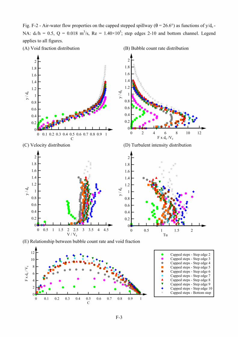
F-3
Fig. F-2 - Air-water flow properties on the capped stepped spillway (θ = 26.6°) as functions of y/dc -
NA: dc/h = 0.5, Q = 0.018 m3/s, Re = 1.40×10⁵; step edges 2-10 and bottom channel. Legend
applies to all figures.
(A) Void fraction distribution (B) Bubble count rate distribution
C
y / d
c
0 0.1 0.2 0.3 0.4 0.5 0.6 0.7 0.8 0.9 10
0.2
0.4
0.6
0.8
1
1.2
1.4
1.6
1.8
2
F x dc /Vc
y / d
c
0 2 4 6 8 10 120
0.2
0.4
0.6
0.8
1
1.2
1.4
1.6
1.8
2
(C) Velocity distribution (D) Turbulent intensity distribution
V / Vc
y / d
c
0 0.5 1 1.5 2 2.5 3 3.5 4 4.50
0.2
0.4
0.6
0.8
1
1.2
1.4
1.6
1.8
2
Tu
y / d
c
0 0.5 1 1.5 20
0.2
0.4
0.6
0.8
1
1.2
1.4
1.6
1.8
2
(E) Relationship between bubble count rate and void fraction
C
F x
dc
/ Vc
0 0.1 0.2 0.3 0.4 0.5 0.6 0.7 0.8 0.9 10
2
4
6
8
10
12 Capped steps - Step edge 2Capped steps - Step edge 3Capped steps - Step edge 4Capped steps - Step edge 5Capped steps - Step edge 6Capped steps - Step edge 7Capped steps - Step edge 8Capped steps - Step edge 9Capped steps - Step edge 10Capped steps - Bottom step
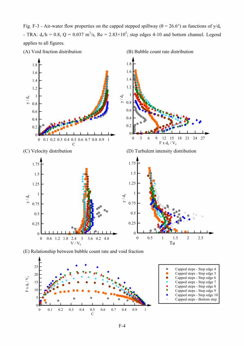
F-4
Fig. F-3 - Air-water flow properties on the capped stepped spillway (θ = 26.6°) as functions of y/dc
- TRA: dc/h = 0.8, Q = 0.037 m3/s, Re = 2.83×10⁵; step edges 4-10 and bottom channel. Legend
applies to all figures.
(A) Void fraction distribution (B) Bubble count rate distribution
C
y / d
c
0 0.1 0.2 0.3 0.4 0.5 0.6 0.7 0.8 0.9 10
0.2
0.4
0.6
0.8
1
1.2
1.4
1.6
1.8
F x dc / Vc
y / d
c
0 3 6 9 12 15 18 21 24 270
0.2
0.4
0.6
0.8
1
1.2
1.4
1.6
1.8
(C) Velocity distribution (D) Turbulent intensity distribution
V / Vc
y / d
c
0 0.6 1.2 1.8 2.4 3 3.6 4.2 4.80
0.25
0.5
0.75
1
1.25
1.5
1.75
Tu
y / d
c
0 0.5 1 1.5 2 2.50
0.25
0.5
0.75
1
1.25
1.5
1.75
(E) Relationship between bubble count rate and void fraction
C
F x
dc
/ Vc
0 0.1 0.2 0.3 0.4 0.5 0.6 0.7 0.8 0.9 10
5
10
15
20
25Capped steps - Step edge 4Capped steps - Step edge 5Capped steps - Step edge 6Capped steps - Step edge 7Capped steps - Step edge 8Capped steps - Step edge 9Capped steps - Step edge 10Capped steps - Bottom step
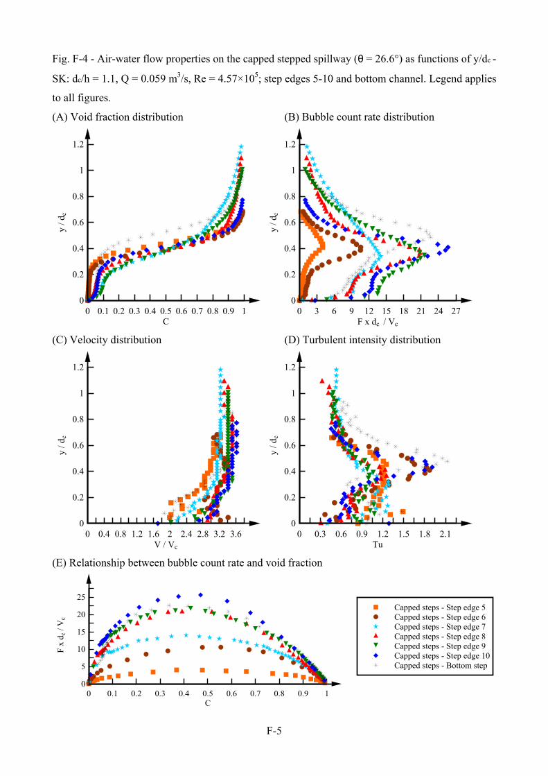
F-5
Fig. F-4 - Air-water flow properties on the capped stepped spillway (θ = 26.6°) as functions of y/dc -
SK: dc/h = 1.1, Q = 0.059 m3/s, Re = 4.57×10⁵; step edges 5-10 and bottom channel. Legend applies
to all figures.
(A) Void fraction distribution (B) Bubble count rate distribution
C
y / d
c
0 0.1 0.2 0.3 0.4 0.5 0.6 0.7 0.8 0.9 10
0.2
0.4
0.6
0.8
1
1.2
F x dc / Vc
y / d
c
0 3 6 9 12 15 18 21 24 270
0.2
0.4
0.6
0.8
1
1.2
(C) Velocity distribution (D) Turbulent intensity distribution
V / Vc
y / d
c
0 0.4 0.8 1.2 1.6 2 2.4 2.8 3.2 3.60
0.2
0.4
0.6
0.8
1
1.2
Tu
y / d
c
0 0.3 0.6 0.9 1.2 1.5 1.8 2.10
0.2
0.4
0.6
0.8
1
1.2
(E) Relationship between bubble count rate and void fraction
C
F x
dc
/ Vc
0 0.1 0.2 0.3 0.4 0.5 0.6 0.7 0.8 0.9 10
5
10
15
20
25Capped steps - Step edge 5Capped steps - Step edge 6Capped steps - Step edge 7Capped steps - Step edge 8Capped steps - Step edge 9Capped steps - Step edge 10Capped steps - Bottom step
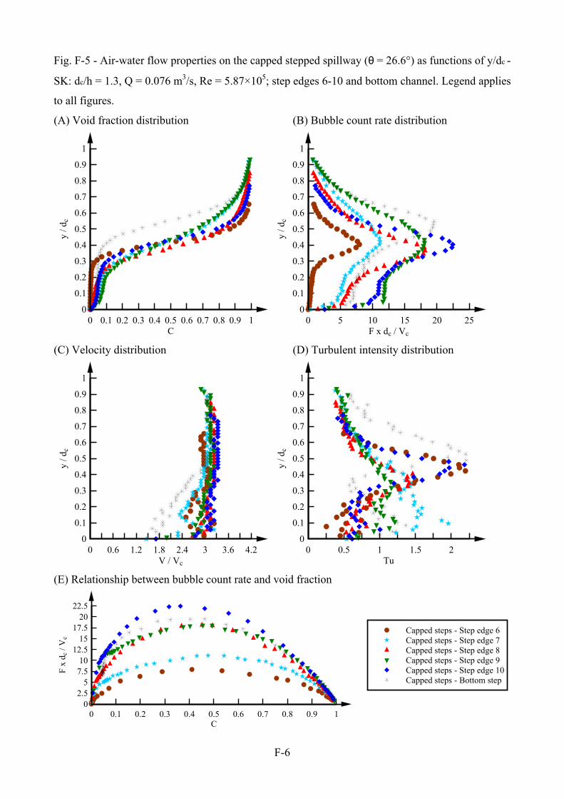
F-6
Fig. F-5 - Air-water flow properties on the capped stepped spillway (θ = 26.6°) as functions of y/dc -
SK: dc/h = 1.3, Q = 0.076 m3/s, Re = 5.87×10⁵; step edges 6-10 and bottom channel. Legend applies
to all figures.
(A) Void fraction distribution (B) Bubble count rate distribution
C
y / d
c
0 0.1 0.2 0.3 0.4 0.5 0.6 0.7 0.8 0.9 10
0.1
0.2
0.3
0.4
0.5
0.6
0.7
0.8
0.9
1
F x dc / Vc
y / d
c
0 5 10 15 20 250
0.1
0.2
0.3
0.4
0.5
0.6
0.7
0.8
0.9
1
(C) Velocity distribution (D) Turbulent intensity distribution
V / Vc
y / d
c
0 0.6 1.2 1.8 2.4 3 3.6 4.20
0.1
0.2
0.3
0.4
0.5
0.6
0.7
0.8
0.9
1
Tu
y / d
c
0 0.5 1 1.5 20
0.1
0.2
0.3
0.4
0.5
0.6
0.7
0.8
0.9
1
(E) Relationship between bubble count rate and void fraction
C
F x
dc
/ Vc
0 0.1 0.2 0.3 0.4 0.5 0.6 0.7 0.8 0.9 10
2.55
7.510
12.515
17.520
22.5
Capped steps - Step edge 6Capped steps - Step edge 7Capped steps - Step edge 8Capped steps - Step edge 9Capped steps - Step edge 10Capped steps - Bottom step
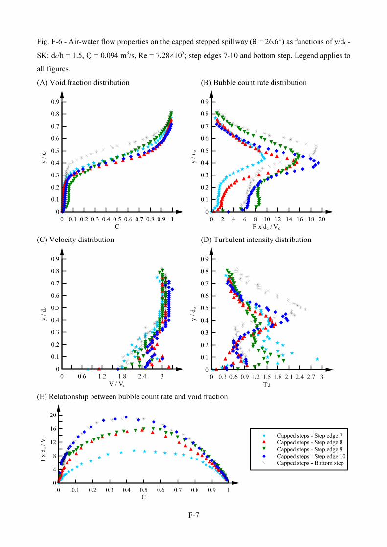
F-7
Fig. F-6 - Air-water flow properties on the capped stepped spillway (θ = 26.6°) as functions of y/dc -
SK: dc/h = 1.5, Q = 0.094 m3/s, Re = 7.28×10⁵; step edges 7-10 and bottom step. Legend applies to
all figures.
(A) Void fraction distribution (B) Bubble count rate distribution
C
y / d
c
0 0.1 0.2 0.3 0.4 0.5 0.6 0.7 0.8 0.9 10
0.1
0.2
0.3
0.4
0.5
0.6
0.7
0.8
0.9
F x dc / Vc
y / d
c
0 2 4 6 8 10 12 14 16 18 200
0.1
0.2
0.3
0.4
0.5
0.6
0.7
0.8
0.9
(C) Velocity distribution (D) Turbulent intensity distribution
V / Vc
y / d
c
0 0.6 1.2 1.8 2.4 30
0.1
0.2
0.3
0.4
0.5
0.6
0.7
0.8
0.9
Tu
y / d
c
0 0.3 0.6 0.9 1.2 1.5 1.8 2.1 2.4 2.7 30
0.1
0.2
0.3
0.4
0.5
0.6
0.7
0.8
0.9
(E) Relationship between bubble count rate and void fraction
C
F x
dc
/ Vc
0 0.1 0.2 0.3 0.4 0.5 0.6 0.7 0.8 0.9 10
4
8
12
16
20
Capped steps - Step edge 7Capped steps - Step edge 8Capped steps - Step edge 9Capped steps - Step edge 10Capped steps - Bottom step
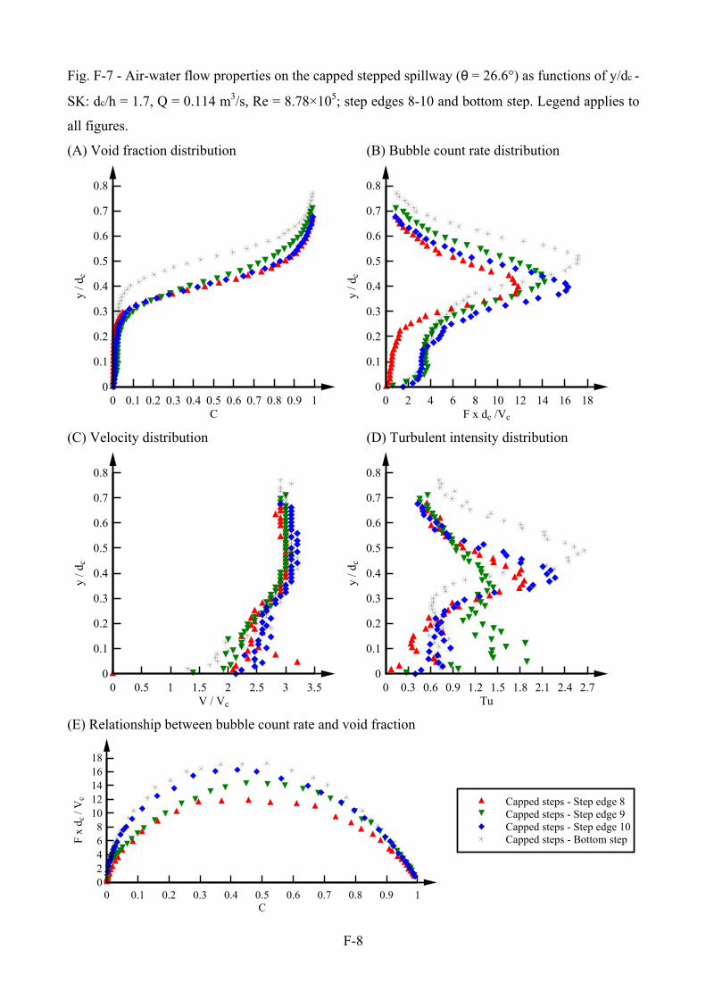
F-8
Fig. F-7 - Air-water flow properties on the capped stepped spillway (θ = 26.6°) as functions of y/dc -
SK: dc/h = 1.7, Q = 0.114 m3/s, Re = 8.78×10⁵; step edges 8-10 and bottom step. Legend applies to
all figures.
(A) Void fraction distribution (B) Bubble count rate distribution
C
y / d
c
0 0.1 0.2 0.3 0.4 0.5 0.6 0.7 0.8 0.9 10
0.1
0.2
0.3
0.4
0.5
0.6
0.7
0.8
F x dc /Vc
y / d
c
0 2 4 6 8 10 12 14 16 180
0.1
0.2
0.3
0.4
0.5
0.6
0.7
0.8
(C) Velocity distribution (D) Turbulent intensity distribution
V / Vc
y / d
c
0 0.5 1 1.5 2 2.5 3 3.50
0.1
0.2
0.3
0.4
0.5
0.6
0.7
0.8
Tu
y / d
c
0 0.3 0.6 0.9 1.2 1.5 1.8 2.1 2.4 2.70
0.1
0.2
0.3
0.4
0.5
0.6
0.7
0.8
(E) Relationship between bubble count rate and void fraction
C
F x
dc
/ Vc
0 0.1 0.2 0.3 0.4 0.5 0.6 0.7 0.8 0.9 102468
1012141618
Capped steps - Step edge 8Capped steps - Step edge 9Capped steps - Step edge 10Capped steps - Bottom step
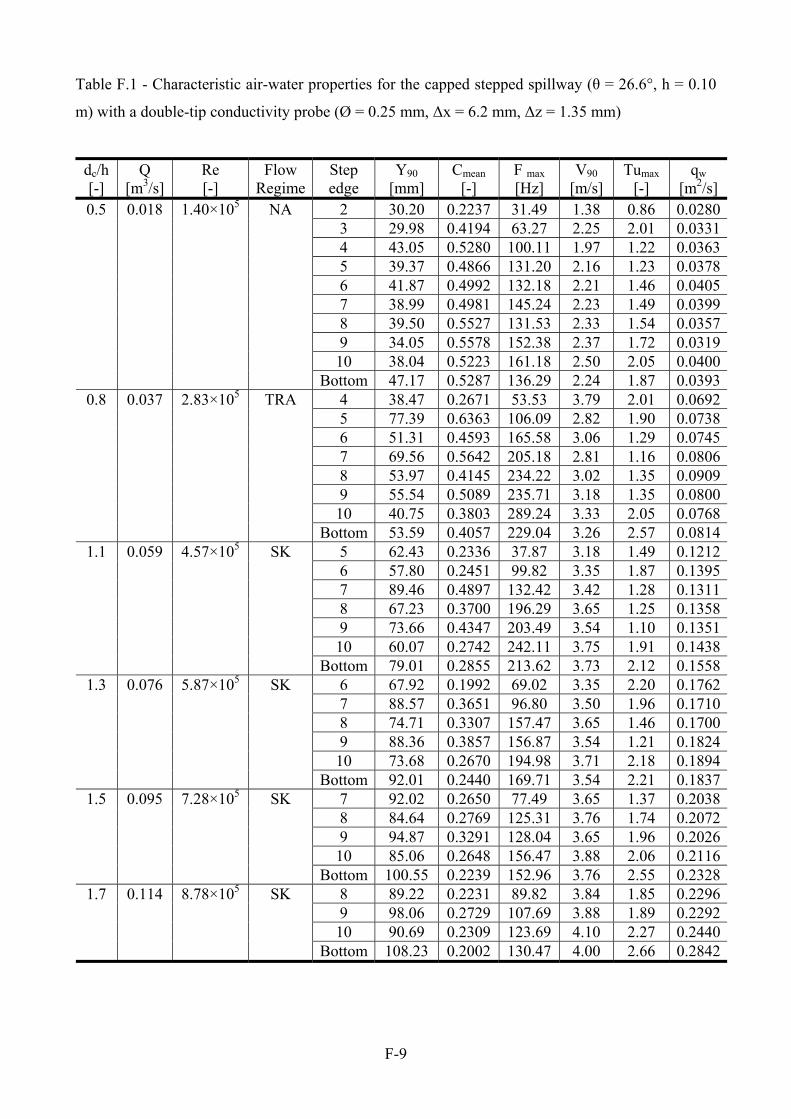
F-9
Table F.1 - Characteristic air-water properties for the capped stepped spillway (θ = 26.6°, h = 0.10
m) with a double-tip conductivity probe (Ø = 0.25 mm, Δx = 6.2 mm, Δz = 1.35 mm)
dc/h [-]
Q [m3/s]
Re [-]
Flow Regime
Step edge
Y90 [mm]
Cmean [-]
F max
[Hz] V90
[m/s] Tumax
[-] qw
[m2/s] 2 30.20 0.2237 31.49 1.38 0.86 0.02803 29.98 0.4194 63.27 2.25 2.01 0.03314 43.05 0.5280 100.11 1.97 1.22 0.03635 39.37 0.4866 131.20 2.16 1.23 0.03786 41.87 0.4992 132.18 2.21 1.46 0.04057 38.99 0.4981 145.24 2.23 1.49 0.03998 39.50 0.5527 131.53 2.33 1.54 0.03579 34.05 0.5578 152.38 2.37 1.72 0.031910 38.04 0.5223 161.18 2.50 2.05 0.0400
0.5 0.018 1.40×10⁵ NA
Bottom 47.17 0.5287 136.29 2.24 1.87 0.03934 38.47 0.2671 53.53 3.79 2.01 0.06925 77.39 0.6363 106.09 2.82 1.90 0.07386 51.31 0.4593 165.58 3.06 1.29 0.07457 69.56 0.5642 205.18 2.81 1.16 0.08068 53.97 0.4145 234.22 3.02 1.35 0.09099 55.54 0.5089 235.71 3.18 1.35 0.080010 40.75 0.3803 289.24 3.33 2.05 0.0768
0.8 0.037 2.83×10⁵ TRA
Bottom 53.59 0.4057 229.04 3.26 2.57 0.08145 62.43 0.2336 37.87 3.18 1.49 0.12126 57.80 0.2451 99.82 3.35 1.87 0.13957 89.46 0.4897 132.42 3.42 1.28 0.13118 67.23 0.3700 196.29 3.65 1.25 0.13589 73.66 0.4347 203.49 3.54 1.10 0.135110 60.07 0.2742 242.11 3.75 1.91 0.1438
1.1 0.059 4.57×10⁵ SK
Bottom 79.01 0.2855 213.62 3.73 2.12 0.15586 67.92 0.1992 69.02 3.35 2.20 0.17627 88.57 0.3651 96.80 3.50 1.96 0.17108 74.71 0.3307 157.47 3.65 1.46 0.17009 88.36 0.3857 156.87 3.54 1.21 0.182410 73.68 0.2670 194.98 3.71 2.18 0.1894
1.3 0.076 5.87×10⁵ SK
Bottom 92.01 0.2440 169.71 3.54 2.21 0.18377 92.02 0.2650 77.49 3.65 1.37 0.20388 84.64 0.2769 125.31 3.76 1.74 0.20729 94.87 0.3291 128.04 3.65 1.96 0.202610 85.06 0.2648 156.47 3.88 2.06 0.2116
1.5 0.095
7.28×10⁵ SK
Bottom 100.55 0.2239 152.96 3.76 2.55 0.23288 89.22 0.2231 89.82 3.84 1.85 0.22969 98.06 0.2729 107.69 3.88 1.89 0.229210 90.69 0.2309 123.69 4.10 2.27 0.2440
1.7 0.114 8.78×10⁵ SK
Bottom 108.23 0.2002 130.47 4.00 2.66 0.2842
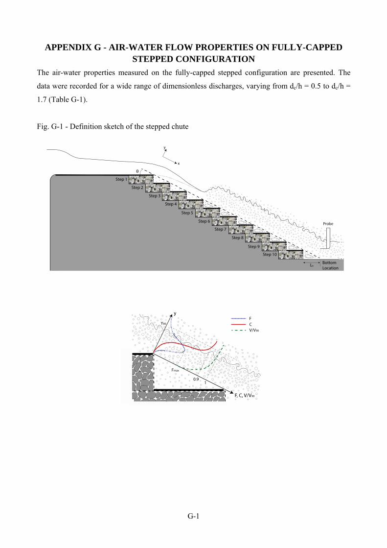
G-1
APPENDIX G - AIR-WATER FLOW PROPERTIES ON FULLY-CAPPED STEPPED CONFIGURATION
The air-water properties measured on the fully-capped stepped configuration are presented. The
data were recorded for a wide range of dimensionless discharges, varying from dc/h = 0.5 to dc/h =
1.7 (Table G-1).
Fig. G-1 - Definition sketch of the stepped chute

G-2
Notation
C void fraction defined as the volume of air per unit volume;
Cmean depth averaged void fraction defined in terms of Y90: Cmean = 1 - d/Y90;
dc critical flow depth (m);
F bubble count rate (Hz) defined as the number of detected air bubbles per unit time;
Fmax maximum bubble count rate (Hz) in a cross-section;
h vertical step height (m);
Q water discharge (m3/s);
qw water discharge per unit width calculated from the integration of the measured void
fraction and velocity profiles:
90Y
0
w dyVC1q
Re Reynolds number defined in terms of hydraulic diameter;
Tu turbulence intensity;
Tumax maximum turbulence intensity in a cross section;
V interfacial velocity (m/s);
V90 interfacial velocity (m/s) at y = Y90;
y distance (m) perpendicular to the pseudo-bottom bottom formed by the step edges;
Y90 characteristic distance (m) where the void fraction equals 0.90;
Δx streamwise distance (m) between probe tips;
Δz transversal distance (m) between probe tips;
Ø diameter (m) of inner probe sensor;
θ chute slope;
Abbreviations
NA nappe flow regime;
TRA transition flow regime;
SK skimming flow regime.
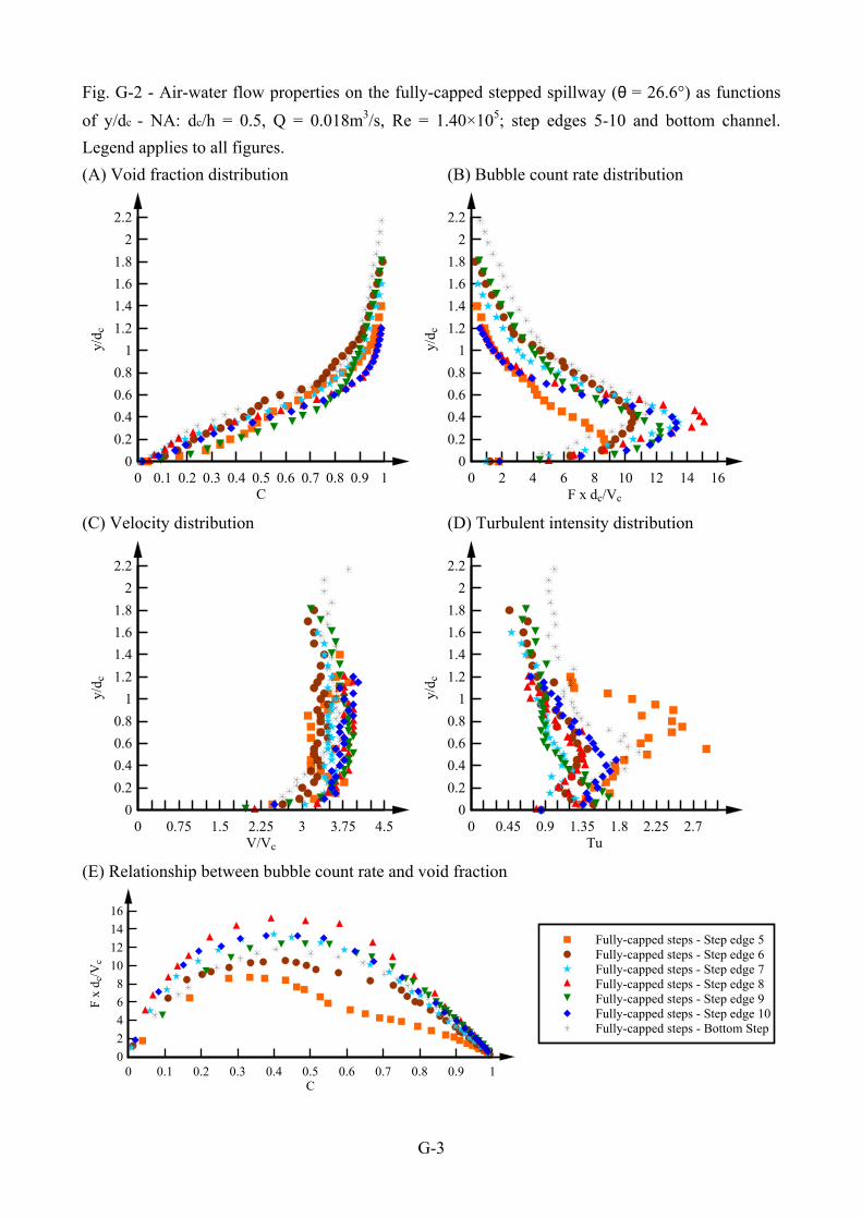
G-3
Fig. G-2 - Air-water flow properties on the fully-capped stepped spillway (θ = 26.6°) as functions
of y/dc - NA: dc/h = 0.5, Q = 0.018m3/s, Re = 1.40×10⁵; step edges 5-10 and bottom channel.
Legend applies to all figures.
(A) Void fraction distribution (B) Bubble count rate distribution
C
y/d c
0 0.1 0.2 0.3 0.4 0.5 0.6 0.7 0.8 0.9 10
0.2
0.4
0.6
0.8
1
1.2
1.4
1.6
1.8
2
2.2
F x dc/Vc
y/d c
0 2 4 6 8 10 12 14 160
0.2
0.4
0.6
0.8
1
1.2
1.4
1.6
1.8
2
2.2
(C) Velocity distribution (D) Turbulent intensity distribution
V/Vc
y/d c
0 0.75 1.5 2.25 3 3.75 4.50
0.2
0.4
0.6
0.8
1
1.2
1.4
1.6
1.8
2
2.2
Tu
y/d c
0 0.45 0.9 1.35 1.8 2.25 2.70
0.2
0.4
0.6
0.8
1
1.2
1.4
1.6
1.8
2
2.2
(E) Relationship between bubble count rate and void fraction
C
F x
dc/
Vc
0 0.1 0.2 0.3 0.4 0.5 0.6 0.7 0.8 0.9 10
2
4
6
8
10
12
14
16
Fully-capped steps - Step edge 5Fully-capped steps - Step edge 6Fully-capped steps - Step edge 7Fully-capped steps - Step edge 8Fully-capped steps - Step edge 9Fully-capped steps - Step edge 10Fully-capped steps - Bottom Step
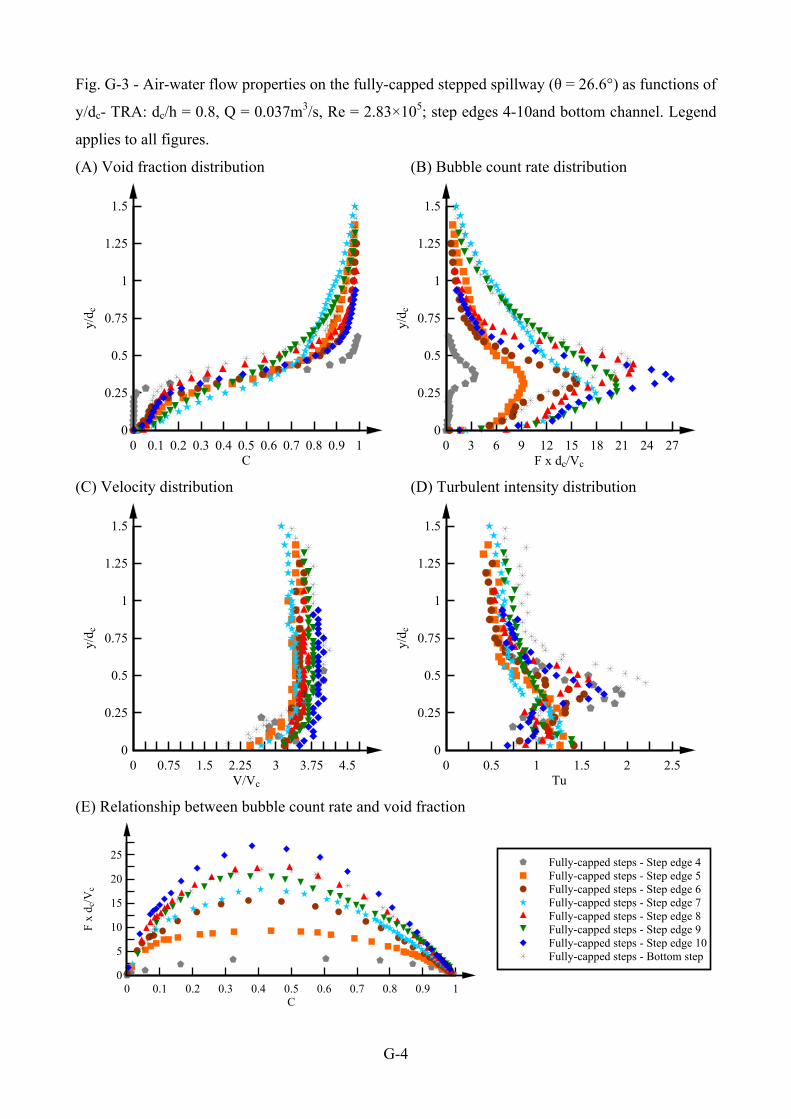
G-4
Fig. G-3 - Air-water flow properties on the fully-capped stepped spillway (θ = 26.6°) as functions of
y/dc- TRA: dc/h = 0.8, Q = 0.037m3/s, Re = 2.83×10⁵; step edges 4-10and bottom channel. Legend
applies to all figures.
(A) Void fraction distribution (B) Bubble count rate distribution
C
y/d c
0 0.1 0.2 0.3 0.4 0.5 0.6 0.7 0.8 0.9 10
0.25
0.5
0.75
1
1.25
1.5
F x dc/Vc
y/d c
0 3 6 9 12 15 18 21 24 270
0.25
0.5
0.75
1
1.25
1.5
(C) Velocity distribution (D) Turbulent intensity distribution
V/Vc
y/d c
0 0.75 1.5 2.25 3 3.75 4.50
0.25
0.5
0.75
1
1.25
1.5
Tu
y/d c
0 0.5 1 1.5 2 2.50
0.25
0.5
0.75
1
1.25
1.5
(E) Relationship between bubble count rate and void fraction
C
F x
dc/
Vc
0 0.1 0.2 0.3 0.4 0.5 0.6 0.7 0.8 0.9 10
5
10
15
20
25Fully-capped steps - Step edge 4Fully-capped steps - Step edge 5Fully-capped steps - Step edge 6Fully-capped steps - Step edge 7Fully-capped steps - Step edge 8Fully-capped steps - Step edge 9Fully-capped steps - Step edge 10Fully-capped steps - Bottom step
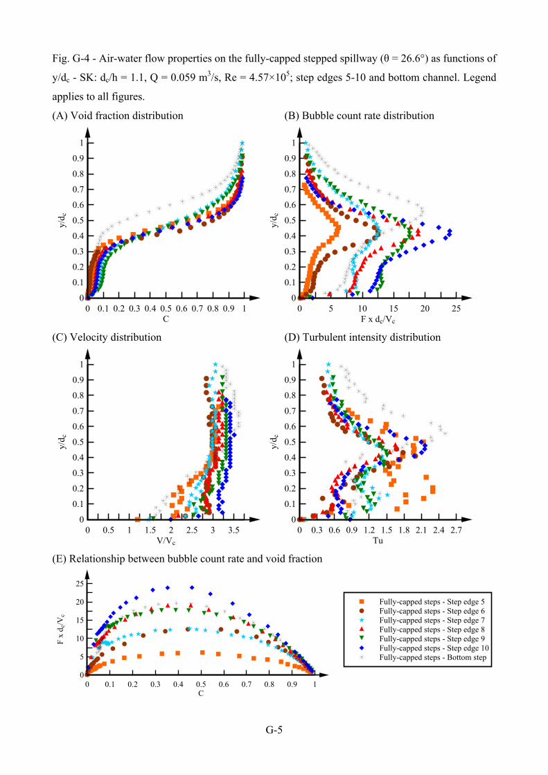
G-5
Fig. G-4 - Air-water flow properties on the fully-capped stepped spillway (θ = 26.6°) as functions of
y/dc - SK: dc/h = 1.1, Q = 0.059 m3/s, Re = 4.57×10⁵; step edges 5-10 and bottom channel. Legend
applies to all figures.
(A) Void fraction distribution (B) Bubble count rate distribution
C
y/d c
0 0.1 0.2 0.3 0.4 0.5 0.6 0.7 0.8 0.9 10
0.1
0.2
0.3
0.4
0.5
0.6
0.7
0.8
0.9
1
F x dc/Vc
y/d c
0 5 10 15 20 250
0.1
0.2
0.3
0.4
0.5
0.6
0.7
0.8
0.9
1
(C) Velocity distribution (D) Turbulent intensity distribution
V/Vc
y/d c
0 0.5 1 1.5 2 2.5 3 3.50
0.1
0.2
0.3
0.4
0.5
0.6
0.7
0.8
0.9
1
Tu
y/d c
0 0.3 0.6 0.9 1.2 1.5 1.8 2.1 2.4 2.70
0.1
0.2
0.3
0.4
0.5
0.6
0.7
0.8
0.9
1
(E) Relationship between bubble count rate and void fraction
C
F x
dc/
Vc
0 0.1 0.2 0.3 0.4 0.5 0.6 0.7 0.8 0.9 10
5
10
15
20
25
Fully-capped steps - Step edge 5Fully-capped steps - Step edge 6Fully-capped steps - Step edge 7Fully-capped steps - Step edge 8Fully-capped steps - Step edge 9Fully-capped steps - Step edge 10Fully-capped steps - Bottom step
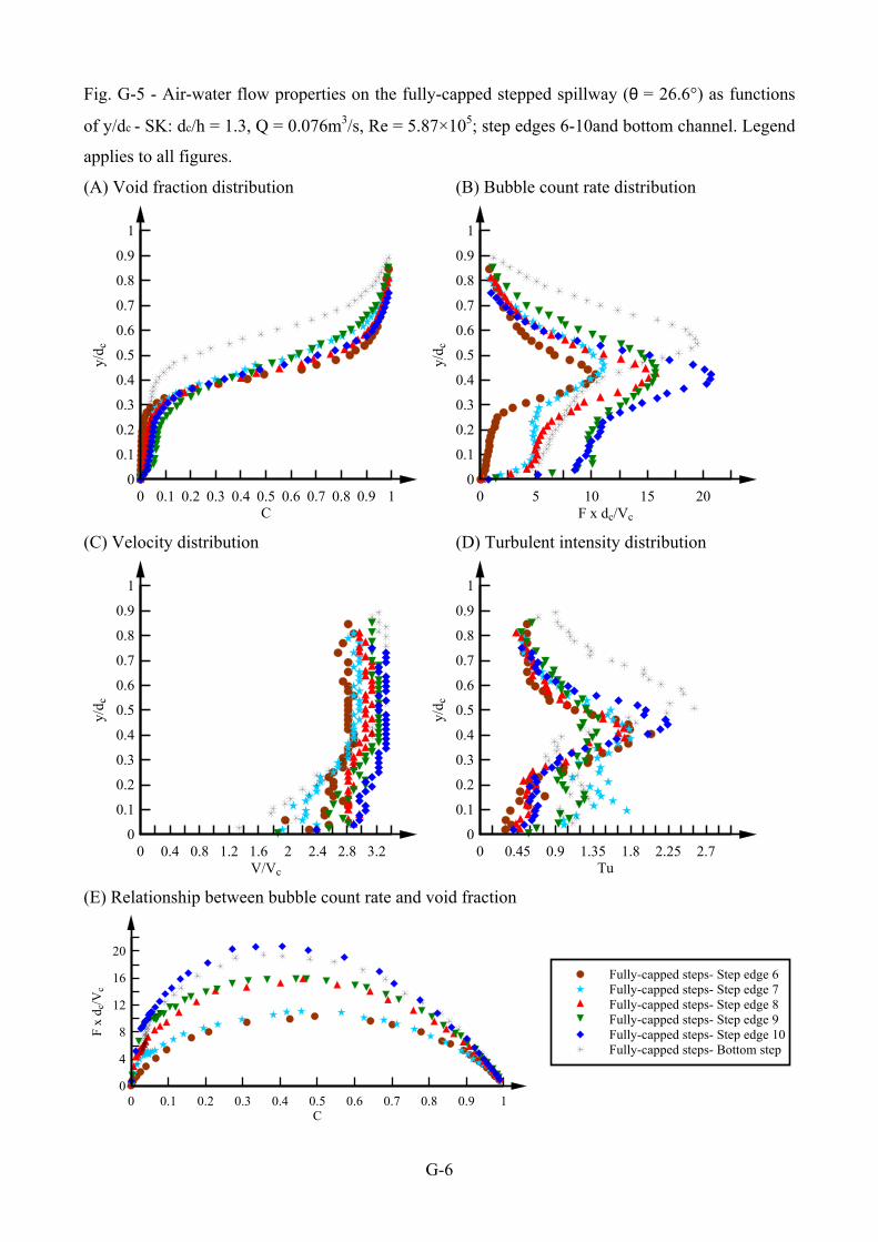
G-6
Fig. G-5 - Air-water flow properties on the fully-capped stepped spillway (θ = 26.6°) as functions
of y/dc - SK: dc/h = 1.3, Q = 0.076m3/s, Re = 5.87×10⁵; step edges 6-10and bottom channel. Legend
applies to all figures.
(A) Void fraction distribution (B) Bubble count rate distribution
C
y/d c
0 0.1 0.2 0.3 0.4 0.5 0.6 0.7 0.8 0.9 10
0.1
0.2
0.3
0.4
0.5
0.6
0.7
0.8
0.9
1
F x dc/Vc
y/d c
0 5 10 15 200
0.1
0.2
0.3
0.4
0.5
0.6
0.7
0.8
0.9
1
(C) Velocity distribution (D) Turbulent intensity distribution
V/Vc
y/d c
0 0.4 0.8 1.2 1.6 2 2.4 2.8 3.20
0.1
0.2
0.3
0.4
0.5
0.6
0.7
0.8
0.9
1
Tu
y/d c
0 0.45 0.9 1.35 1.8 2.25 2.70
0.1
0.2
0.3
0.4
0.5
0.6
0.7
0.8
0.9
1
(E) Relationship between bubble count rate and void fraction
C
F x
dc/
Vc
0 0.1 0.2 0.3 0.4 0.5 0.6 0.7 0.8 0.9 10
4
8
12
16
20
Fully-capped steps- Step edge 6Fully-capped steps- Step edge 7Fully-capped steps- Step edge 8Fully-capped steps- Step edge 9Fully-capped steps- Step edge 10Fully-capped steps- Bottom step
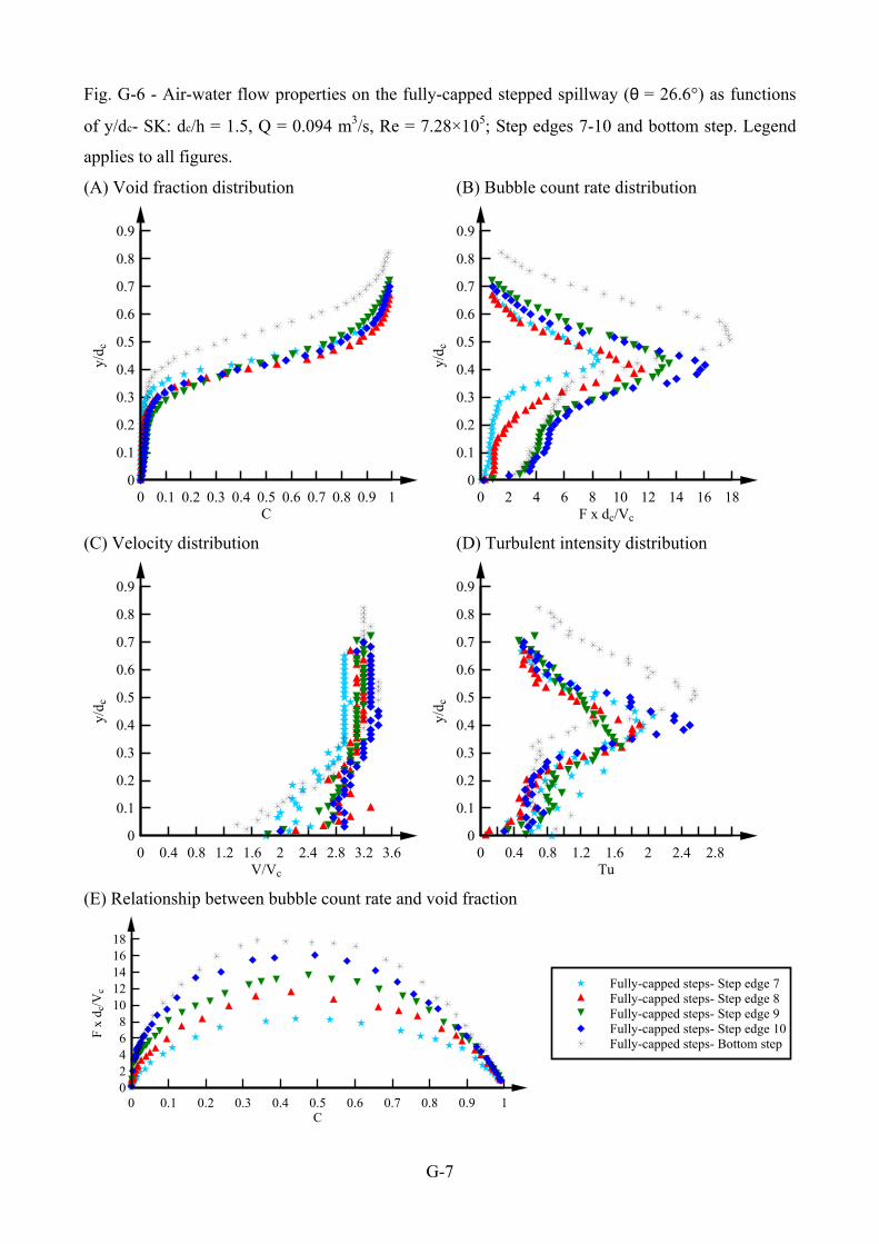
G-7
Fig. G-6 - Air-water flow properties on the fully-capped stepped spillway (θ = 26.6°) as functions
of y/dc- SK: dc/h = 1.5, Q = 0.094 m3/s, Re = 7.28×10⁵; Step edges 7-10 and bottom step. Legend
applies to all figures.
(A) Void fraction distribution (B) Bubble count rate distribution
C
y/d c
0 0.1 0.2 0.3 0.4 0.5 0.6 0.7 0.8 0.9 10
0.1
0.2
0.3
0.4
0.5
0.6
0.7
0.8
0.9
F x dc/Vc
y/d c
0 2 4 6 8 10 12 14 16 180
0.1
0.2
0.3
0.4
0.5
0.6
0.7
0.8
0.9
(C) Velocity distribution (D) Turbulent intensity distribution
V/Vc
y/d c
0 0.4 0.8 1.2 1.6 2 2.4 2.8 3.2 3.60
0.1
0.2
0.3
0.4
0.5
0.6
0.7
0.8
0.9
Tu
y/d c
0 0.4 0.8 1.2 1.6 2 2.4 2.80
0.1
0.2
0.3
0.4
0.5
0.6
0.7
0.8
0.9
(E) Relationship between bubble count rate and void fraction
C
F x
dc/
Vc
0 0.1 0.2 0.3 0.4 0.5 0.6 0.7 0.8 0.9 102468
1012141618
Fully-capped steps- Step edge 7Fully-capped steps- Step edge 8Fully-capped steps- Step edge 9Fully-capped steps- Step edge 10Fully-capped steps- Bottom step
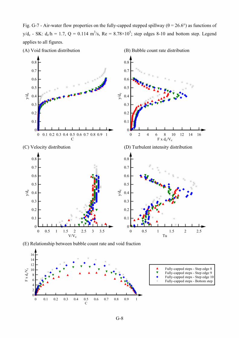
G-8
Fig. G-7 - Air-water flow properties on the fully-capped stepped spillway (θ = 26.6°) as functions of
y/dc - SK: dc/h = 1.7, Q = 0.114 m3/s, Re = 8.78×10⁵; step edges 8-10 and bottom step. Legend
applies to all figures.
(A) Void fraction distribution (B) Bubble count rate distribution
C
y/d c
0 0.1 0.2 0.3 0.4 0.5 0.6 0.7 0.8 0.9 10
0.1
0.2
0.3
0.4
0.5
0.6
0.7
0.8
F x dc/Vc
y/d c
0 2 4 6 8 10 12 14 160
0.1
0.2
0.3
0.4
0.5
0.6
0.7
0.8
(C) Velocity distribution (D) Turbulent intensity distribution
V/Vc
y/d c
0 0.5 1 1.5 2 2.5 3 3.50
0.1
0.2
0.3
0.4
0.5
0.6
0.7
0.8
Tu
y/d c
0 0.5 1 1.5 2 2.50
0.1
0.2
0.3
0.4
0.5
0.6
0.7
0.8
(E) Relationship between bubble count rate and void fraction
C
F x
dc/
Vc
0 0.1 0.2 0.3 0.4 0.5 0.6 0.7 0.8 0.9 10
2
4
6
8
10
12
14
16
Fully-capped steps - Step edge 8Fully-capped steps - Step edge 9Fully-capped steps - Step edge 10Fully-capped steps - Bottom step
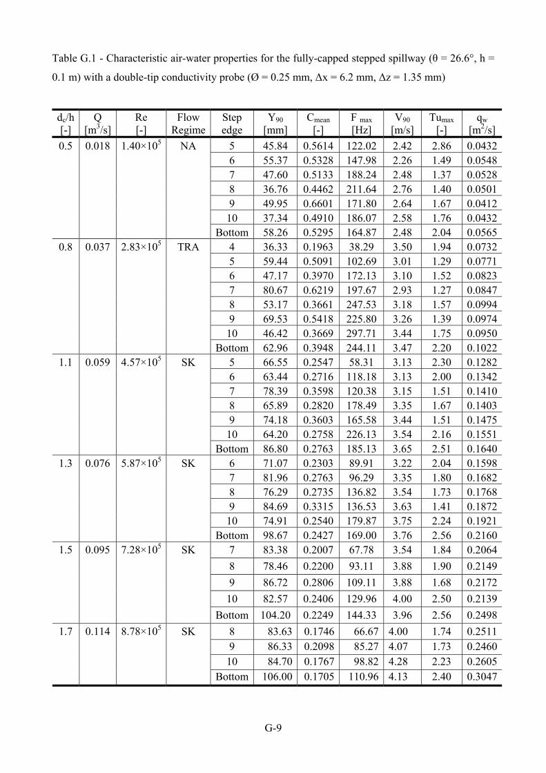
G-9
Table G.1 - Characteristic air-water properties for the fully-capped stepped spillway (θ = 26.6°, h =
0.1 m) with a double-tip conductivity probe (Ø = 0.25 mm, Δx = 6.2 mm, Δz = 1.35 mm)
dc/h [-]
Q [m3/s]
Re [-]
Flow Regime
Step edge
Y90 [mm]
Cmean [-]
F max
[Hz] V90
[m/s] Tumax
[-] qw
[m2/s]
5 45.84 0.5614 122.02 2.42 2.86 0.04326 55.37 0.5328 147.98 2.26 1.49 0.05487 47.60 0.5133 188.24 2.48 1.37 0.05288 36.76 0.4462 211.64 2.76 1.40 0.05019 49.95 0.6601 171.80 2.64 1.67 0.041210 37.34 0.4910 186.07 2.58 1.76 0.0432
0.5 0.018 1.40×10⁵ NA
Bottom 58.26 0.5295 164.87 2.48 2.04 0.05654 36.33 0.1963 38.29 3.50 1.94 0.07325 59.44 0.5091 102.69 3.01 1.29 0.07716 47.17 0.3970 172.13 3.10 1.52 0.08237 80.67 0.6219 197.67 2.93 1.27 0.08478 53.17 0.3661 247.53 3.18 1.57 0.09949 69.53 0.5418 225.80 3.26 1.39 0.097410 46.42 0.3669 297.71 3.44 1.75 0.0950
0.8 0.037 2.83×10⁵ TRA
Bottom 62.96 0.3948 244.11 3.47 2.20 0.10225 66.55 0.2547 58.31 3.13 2.30 0.12826 63.44 0.2716 118.18 3.13 2.00 0.13427 78.39 0.3598 120.38 3.15 1.51 0.14108 65.89 0.2820 178.49 3.35 1.67 0.14039 74.18 0.3603 165.58 3.44 1.51 0.147510 64.20 0.2758 226.13 3.54 2.16 0.1551
1.1 0.059 4.57×10⁵ SK
Bottom 86.80 0.2763 185.13 3.65 2.51 0.16406 71.07 0.2303 89.91 3.22 2.04 0.15987 81.96 0.2763 96.29 3.35 1.80 0.16828 76.29 0.2735 136.82 3.54 1.73 0.17689 84.69 0.3315 136.53 3.63 1.41 0.187210 74.91 0.2540 179.87 3.75 2.24 0.1921
1.3 0.076 5.87×10⁵ SK
Bottom 98.67 0.2427 169.00 3.76 2.56 0.21607 83.38 0.2007 67.78 3.54 1.84 0.2064
8 78.46 0.2200 93.11 3.88 1.90 0.2149
9 86.72 0.2806 109.11 3.88 1.68 0.2172
10 82.57 0.2406 129.96 4.00 2.50 0.2139
1.5 0.095
7.28×10⁵ SK
Bottom 104.20 0.2249 144.33 3.96 2.56 0.2498
8 83.63 0.1746 66.67 4.00 1.74 0.25119 86.33 0.2098 85.27 4.07 1.73 0.246010 84.70 0.1767 98.82 4.28 2.23 0.2605
1.7 0.114 8.78×10⁵ SK
Bottom 106.00 0.1705 110.96 4.13 2.40 0.3047
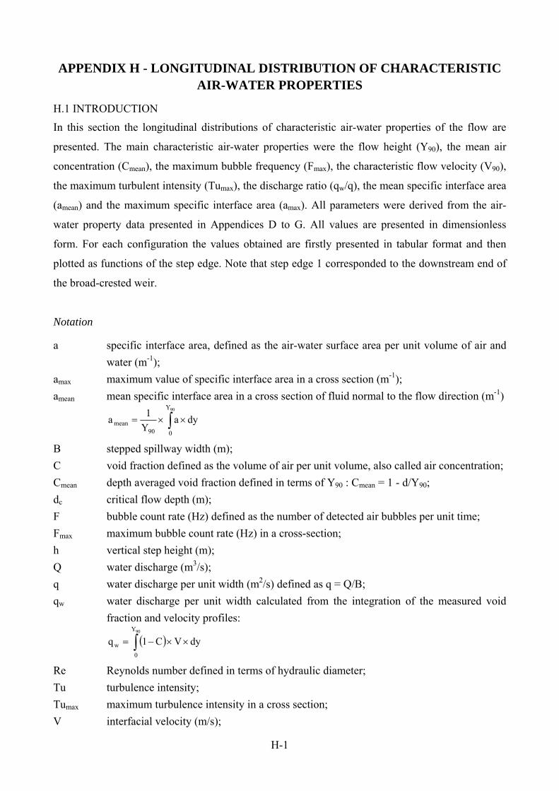
H-1
APPENDIX H - LONGITUDINAL DISTRIBUTION OF CHARACTERISTIC AIR-WATER PROPERTIES
H.1 INTRODUCTION
In this section the longitudinal distributions of characteristic air-water properties of the flow are
presented. The main characteristic air-water properties were the flow height (Y90), the mean air
concentration (Cmean), the maximum bubble frequency (Fmax), the characteristic flow velocity (V90),
the maximum turbulent intensity (Tumax), the discharge ratio (qw/q), the mean specific interface area
(amean) and the maximum specific interface area (amax). All parameters were derived from the air-
water property data presented in Appendices D to G. All values are presented in dimensionless
form. For each configuration the values obtained are firstly presented in tabular format and then
plotted as functions of the step edge. Note that step edge 1 corresponded to the downstream end of
the broad-crested weir.
Notation
a specific interface area, defined as the air-water surface area per unit volume of air and
water (m-1);
amax maximum value of specific interface area in a cross section (m-1);
amean mean specific interface area in a cross section of fluid normal to the flow direction (m-1)
90Y
090mean dya
Y
1a
B stepped spillway width (m);
C void fraction defined as the volume of air per unit volume, also called air concentration;
Cmean depth averaged void fraction defined in terms of Y90 : Cmean = 1 - d/Y90;
dc critical flow depth (m);
F bubble count rate (Hz) defined as the number of detected air bubbles per unit time;
Fmax maximum bubble count rate (Hz) in a cross-section;
h vertical step height (m);
Q water discharge (m3/s);
q water discharge per unit width (m2/s) defined as q = Q/B;
qw water discharge per unit width calculated from the integration of the measured void
fraction and velocity profiles:
90Y
0
w dyVC1q
Re Reynolds number defined in terms of hydraulic diameter;
Tu turbulence intensity;
Tumax maximum turbulence intensity in a cross section;
V interfacial velocity (m/s);
H-2
V90 interfacial velocity (m/s) at y = Y90; Vc critical flow velocity (m/s) defined as cc dgV ;
y distance (m) perpendicular to the pseudo-bottom bottom formed by the step edges;
Y90 characteristic distance (m) where the void fraction equals 0.90;
Δx streamwise distance (m) between probe tips;
Δz transversal distance (m) between probe tips;
Ø diameter (m) of inner probe sensor;
θ chute slope.

H-3
H.2 FLAT STEPPED CONFIGURATION
Table H-1 - Longitudinal distribution of characteristic air-water properties for the measurements on
the flat stepped spillway (θ = 26.6°, h = 0.10 m) with a double-tip conductivity probe (Ø = 0.25
mm, Δx = 6.2 mm, Δz = 1.35 mm)
dc/h [-]
Re [-]
Step edge
Y90/dc [-]
Cmean
[-] Fmax×dc/Vc
[-] qw/q
[-] V90/Vc
[-] Tumax
[-] amax×dc
[-] amean×dc
[-] 3 0.616 0.392 3.612 1.147 3.16 1.76 5.30 2.74 4 0.864 0.532 7.747 0.750 1.72 2.95 12.87 8.04 5 1.855 0.853 5.581 0.984 3.69 0.95 6.18 3.84 6 1.032 0.659 9.398 1.232 4.25 1.70 13.79 7.13 7 0.845 0.525 13.184 1.363 3.54 1.86 22.13 10.93 8 1.220 0.712 11.312 1.151 3.69 2.09 13.46 8.45 9 0.836 0.619 13.877 1.162 4.22 1.96 26.72 11.25
0.5 1.40×10⁵
10 0.970 0.650 13.365 1.163 3.64 1.73 22.34 10.06 4 0.517 0.238 6.004 1.130 3.33 1.49 6.99 2.93 5 0.663 0.417 11.996 1.144 3.27 1.34 14.74 11.69 6 0.749 0.560 16.022 1.007 3.34 1.43 19.49 11.96 7 0.554 0.371 19.656 1.101 3.50 1.82 22.47 15.28 8 0.693 0.494 20.885 1.109 3.48 1.62 23.28 15.79 9 0.684 0.473 22.632 1.082 3.60 1.51 25.22 16.34
0.8 2.83×10⁵
10 0.578 0.399 24.605 1.164 3.78 2.47 26.72 18.58 5 0.504 0.224 5.697 1.049 3.24 3.58 7.06 3.13 6 0.532 0.310 14.037 1.066 3.03 1.72 18.34 9.03 7 0.649 0.377 14.632 1.053 3.10 1.78 19.12 14.69 8 0.584 0.311 20.009 1.144 3.17 1.85 25.35 16.14 9 0.624 0.348 19.632 1.169 3.27 1.97 24.50 18.61
1.1 4.57×10⁵
10 0.572 0.307 24.628 1.238 3.33 2.17 28.88 18.14 5 0.463 0.141 3.149 0.891 2.75 5.77 4.68 1.21 6 0.502 0.233 8.961 0.988 2.80 1.80 13.03 5.24 7 0.558 0.306 12.041 0.975 2.87 2.11 16.67 12.26 8 0.580 0.318 17.730 1.074 2.88 1.86 24.69 15.00 9 0.601 0.346 17.820 1.054 3.01 1.44 24.26 19.32
1.3 5.87×10⁵
10 0.569 0.301 22.645 1.111 3.15 1.78 28.73 19.87 5 0.460 0.102 2.690 - 2.80 3.92 4.01 0.82 6 0.485 0.182 5.806 0.893 2.76 2.35 8.18 2.76 7 0.508 0.236 9.730 0.976 2.92 2.53 13.33 6.75 8 0.527 0.292 14.501 1.046 3.10 2.14 19.86 9.81 9 0.567 0.303 15.798 1.025 3.10 2.03 21.02 15.16
1.5 7.28×10⁵
10 0.565 0.301 20.304 1.025 3.00 1.73 28.12 18.97 6 0.474 0.131 4.084 0.849 2.67 2.43 6.12 1.43 7 0.487 0.194 7.082 0.985 2.91 2.01 9.74 3.64 8 0.487 0.211 11.301 0.985 3.00 2.38 15.37 6.27 9 0.534 0.273 14.036 0.983 3.00 2.08 18.71 10.91
1.7 8.7×10⁵
10 0.545 0.277 17.265 1.078 3.10 2.34 23.02 12.90
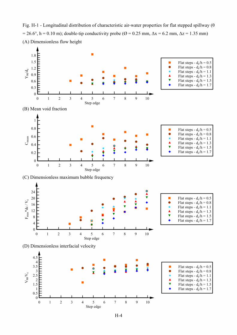
H-4
Fig. H-1 - Longitudinal distribution of characteristic air-water properties for flat stepped spillway (θ
= 26.6°, h = 0.10 m); double-tip conductivity probe (Ø = 0.25 mm, Δx = 6.2 mm, Δz = 1.35 mm)
(A) Dimensionless flow height
Step edge
Y90
/dc
0 1 2 3 4 5 6 7 8 9 100
0.3
0.6
0.9
1.2
1.5
1.8
Flat steps - dc/h = 0.5Flat steps - dc/h = 0.8Flat steps - dc/h = 1.1Flat steps - dc/h = 1.3Flat steps - dc/h = 1.5Flat steps - dc/h = 1.7
(B) Mean void fraction
Step edge
Cm
ean
0 1 2 3 4 5 6 7 8 9 100
0.2
0.4
0.6
0.8
1
Flat steps - dc/h = 0.5Flat steps - dc/h = 0.8Flat steps - dc/h = 1.1Flat steps - dc/h = 1.3Flat steps - dc/h = 1.5Flat steps - dc/h = 1.7
(C) Dimensionless maximum bubble frequency
Step edge
Fm
ax*d
c / V
c
0 1 2 3 4 5 6 7 8 9 100
4
8
12
16
20
24
Flat steps - dc/h = 0.5Flat steps - dc/h = 0.8Flat steps - dc/h = 1.1Flat steps - dc/h = 1.3Flat steps - dc/h = 1.5Flat steps - dc/h = 1.7
(D) Dimensionless interfacial velocity
Step edge
V90
/Vc
0 1 2 3 4 5 6 7 8 9 100
0.51
1.52
2.53
3.54
4.5
Flat steps - dc/h = 0.5Flat steps - dc/h = 0.8Flat steps - dc/h = 1.1Flat steps - dc/h = 1.3Flat steps - dc/h = 1.5Flat steps - dc/h = 1.7
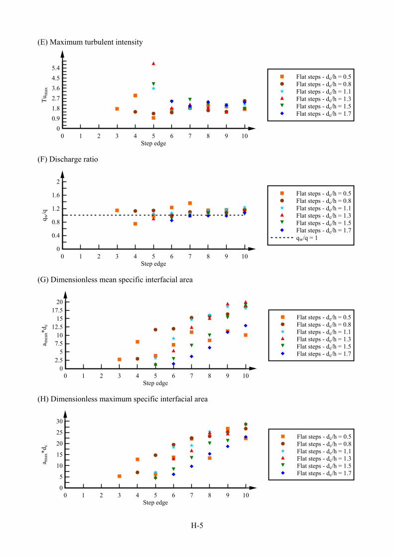
H-5
(E) Maximum turbulent intensity
Step edge
Tu m
ax
0 1 2 3 4 5 6 7 8 9 100
0.9
1.8
2.7
3.6
4.5
5.4Flat steps - dc/h = 0.5Flat steps - dc/h = 0.8Flat steps - dc/h = 1.1Flat steps - dc/h = 1.3Flat steps - dc/h = 1.5Flat steps - dc/h = 1.7
(F) Discharge ratio
Step edge
q w/q
0 1 2 3 4 5 6 7 8 9 100
0.4
0.8
1.2
1.6
2
Flat steps - dc/h = 0.5Flat steps - dc/h = 0.8Flat steps - dc/h = 1.1Flat steps - dc/h = 1.3Flat steps - dc/h = 1.5Flat steps - dc/h = 1.7qw/q = 1
(G) Dimensionless mean specific interfacial area
Step edge
a mea
n*d c
0 1 2 3 4 5 6 7 8 9 100
2.55
7.510
12.515
17.520
Flat steps - dc/h = 0.5Flat steps - dc/h = 0.8Flat steps - dc/h = 1.1Flat steps - dc/h = 1.3Flat steps - dc/h = 1.5Flat steps - dc/h = 1.7
(H) Dimensionless maximum specific interfacial area
Step edge
a max
*dc
0 1 2 3 4 5 6 7 8 9 100
5
10
15
20
25
30
Flat steps - dc/h = 0.5Flat steps - dc/h = 0.8Flat steps - dc/h = 1.1Flat steps - dc/h = 1.3Flat steps - dc/h = 1.5Flat steps - dc/h = 1.7
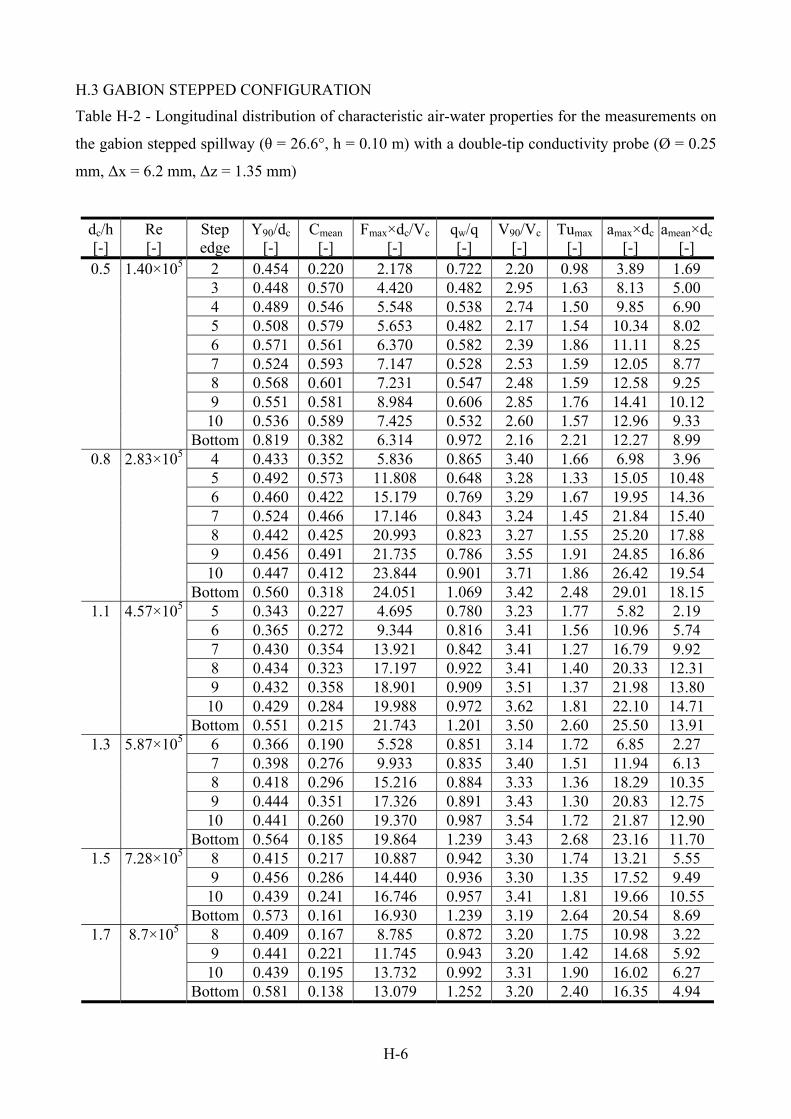
H-6
H.3 GABION STEPPED CONFIGURATION
Table H-2 - Longitudinal distribution of characteristic air-water properties for the measurements on
the gabion stepped spillway (θ = 26.6°, h = 0.10 m) with a double-tip conductivity probe (Ø = 0.25
mm, Δx = 6.2 mm, Δz = 1.35 mm)
dc/h [-]
Re [-]
Step edge
Y90/dc [-]
Cmean [-]
Fmax×dc/Vc
[-] qw/q
[-] V90/Vc
[-] Tumax
[-] amax×dc
[-] amean×dc
[-] 2 0.454 0.220 2.178 0.722 2.20 0.98 3.89 1.69 3 0.448 0.570 4.420 0.482 2.95 1.63 8.13 5.00 4 0.489 0.546 5.548 0.538 2.74 1.50 9.85 6.90 5 0.508 0.579 5.653 0.482 2.17 1.54 10.34 8.02 6 0.571 0.561 6.370 0.582 2.39 1.86 11.11 8.25 7 0.524 0.593 7.147 0.528 2.53 1.59 12.05 8.77 8 0.568 0.601 7.231 0.547 2.48 1.59 12.58 9.25 9 0.551 0.581 8.984 0.606 2.85 1.76 14.41 10.12 10 0.536 0.589 7.425 0.532 2.60 1.57 12.96 9.33
0.5 1.40×10⁵
Bottom 0.819 0.382 6.314 0.972 2.16 2.21 12.27 8.99 4 0.433 0.352 5.836 0.865 3.40 1.66 6.98 3.96 5 0.492 0.573 11.808 0.648 3.28 1.33 15.05 10.48 6 0.460 0.422 15.179 0.769 3.29 1.67 19.95 14.36 7 0.524 0.466 17.146 0.843 3.24 1.45 21.84 15.40 8 0.442 0.425 20.993 0.823 3.27 1.55 25.20 17.88 9 0.456 0.491 21.735 0.786 3.55 1.91 24.85 16.86 10 0.447 0.412 23.844 0.901 3.71 1.86 26.42 19.54
0.8 2.83×10⁵
Bottom 0.560 0.318 24.051 1.069 3.42 2.48 29.01 18.15 5 0.343 0.227 4.695 0.780 3.23 1.77 5.82 2.19 6 0.365 0.272 9.344 0.816 3.41 1.56 10.96 5.74 7 0.430 0.354 13.921 0.842 3.41 1.27 16.79 9.92 8 0.434 0.323 17.197 0.922 3.41 1.40 20.33 12.31 9 0.432 0.358 18.901 0.909 3.51 1.37 21.98 13.80 10 0.429 0.284 19.988 0.972 3.62 1.81 22.10 14.71
1.1 4.57×10⁵
Bottom 0.551 0.215 21.743 1.201 3.50 2.60 25.50 13.91 6 0.366 0.190 5.528 0.851 3.14 1.72 6.85 2.27 7 0.398 0.276 9.933 0.835 3.40 1.51 11.94 6.13 8 0.418 0.296 15.216 0.884 3.33 1.36 18.29 10.35 9 0.444 0.351 17.326 0.891 3.43 1.30 20.83 12.75 10 0.441 0.260 19.370 0.987 3.54 1.72 21.87 12.90
1.3 5.87×10⁵
Bottom 0.564 0.185 19.864 1.239 3.43 2.68 23.16 11.70 8 0.415 0.217 10.887 0.942 3.30 1.74 13.21 5.55 9 0.456 0.286 14.440 0.936 3.30 1.35 17.52 9.49 10 0.439 0.241 16.746 0.957 3.41 1.81 19.66 10.55
1.5 7.28×10⁵
Bottom 0.573 0.161 16.930 1.239 3.19 2.64 20.54 8.69 8 0.409 0.167 8.785 0.872 3.20 1.75 10.98 3.22 9 0.441 0.221 11.745 0.943 3.20 1.42 14.68 5.92 10 0.439 0.195 13.732 0.992 3.31 1.90 16.02 6.27
1.7 8.7×10⁵
Bottom 0.581 0.138 13.079 1.252 3.20 2.40 16.35 4.94
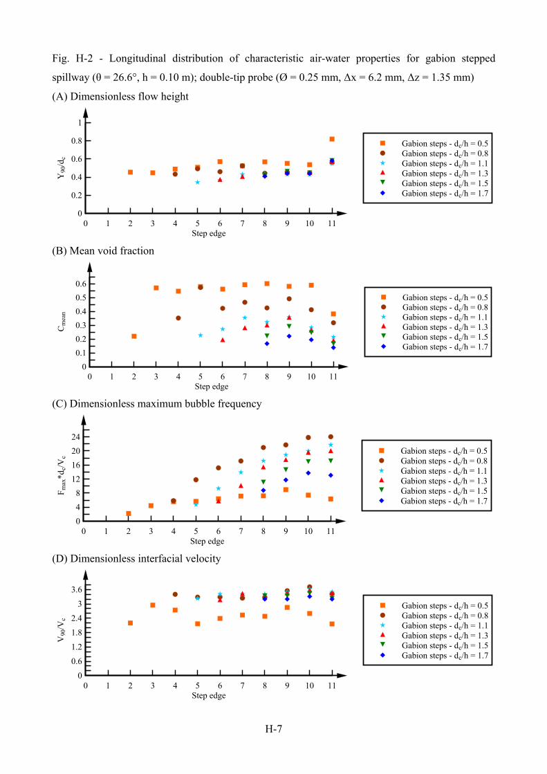
H-7
Fig. H-2 - Longitudinal distribution of characteristic air-water properties for gabion stepped
spillway (θ = 26.6°, h = 0.10 m); double-tip probe (Ø = 0.25 mm, Δx = 6.2 mm, Δz = 1.35 mm)
(A) Dimensionless flow height
Step edge
Y90
/dc
0 1 2 3 4 5 6 7 8 9 10 110
0.2
0.4
0.6
0.8
1
Gabion steps - dc/h = 0.5Gabion steps - dc/h = 0.8Gabion steps - dc/h = 1.1Gabion steps - dc/h = 1.3Gabion steps - dc/h = 1.5Gabion steps - dc/h = 1.7
(B) Mean void fraction
Step edge
Cm
ean
0 1 2 3 4 5 6 7 8 9 10 110
0.1
0.2
0.3
0.4
0.5
0.6
Gabion steps - dc/h = 0.5Gabion steps - dc/h = 0.8Gabion steps - dc/h = 1.1Gabion steps - dc/h = 1.3Gabion steps - dc/h = 1.5Gabion steps - dc/h = 1.7
(C) Dimensionless maximum bubble frequency
Step edge
Fm
ax*d
c/V
c
0 1 2 3 4 5 6 7 8 9 10 110
4
8
12
16
20
24
Gabion steps - dc/h = 0.5Gabion steps - dc/h = 0.8Gabion steps - dc/h = 1.1Gabion steps - dc/h = 1.3Gabion steps - dc/h = 1.5Gabion steps - dc/h = 1.7
(D) Dimensionless interfacial velocity
Step edge
V90
/Vc
0 1 2 3 4 5 6 7 8 9 10 110
0.6
1.2
1.8
2.4
3
3.6
Gabion steps - dc/h = 0.5Gabion steps - dc/h = 0.8Gabion steps - dc/h = 1.1Gabion steps - dc/h = 1.3Gabion steps - dc/h = 1.5Gabion steps - dc/h = 1.7
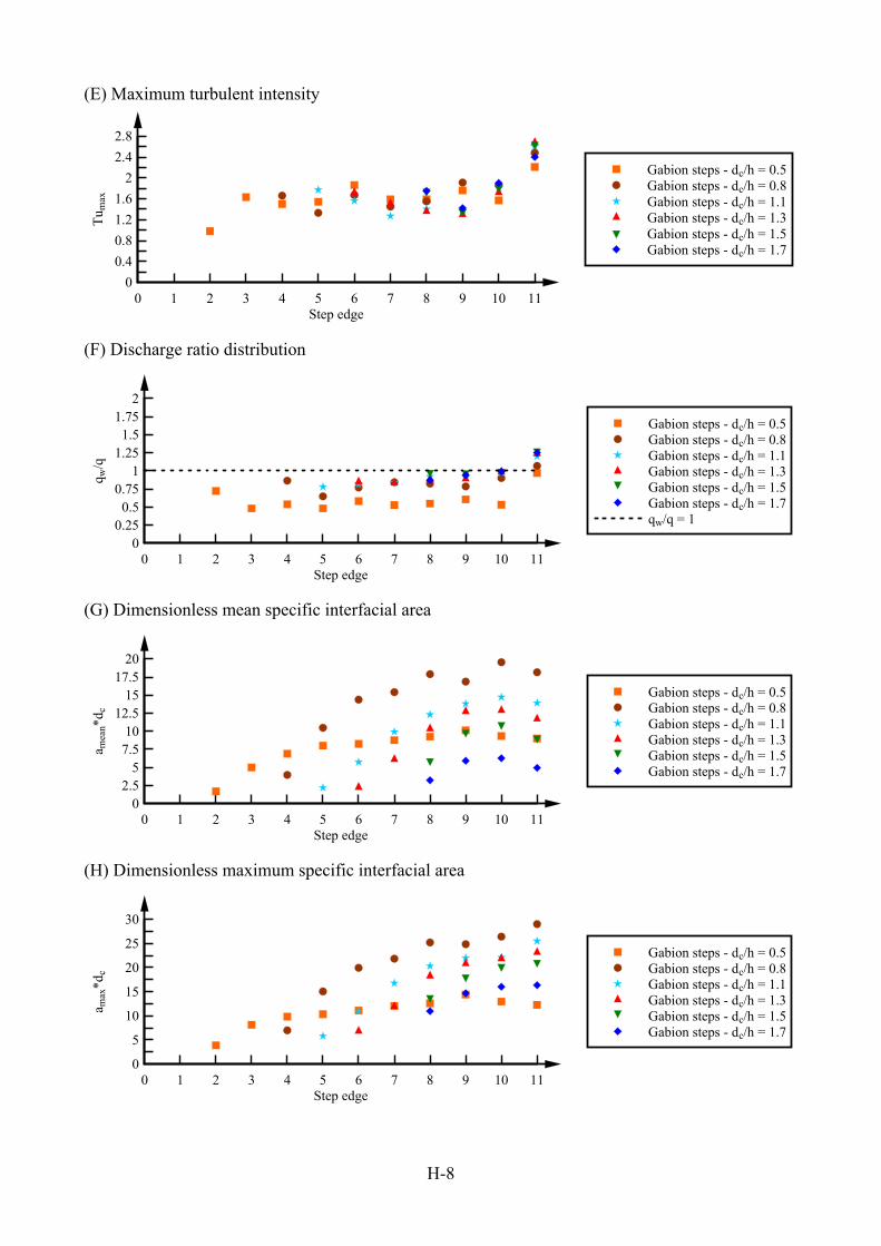
H-8
(E) Maximum turbulent intensity
Step edge
Tu m
ax
0 1 2 3 4 5 6 7 8 9 10 110
0.4
0.8
1.2
1.6
2
2.4
2.8
Gabion steps - dc/h = 0.5Gabion steps - dc/h = 0.8Gabion steps - dc/h = 1.1Gabion steps - dc/h = 1.3Gabion steps - dc/h = 1.5Gabion steps - dc/h = 1.7
(F) Discharge ratio distribution
Step edge
q w/q
0 1 2 3 4 5 6 7 8 9 10 110
0.250.5
0.751
1.251.5
1.752
Gabion steps - dc/h = 0.5Gabion steps - dc/h = 0.8Gabion steps - dc/h = 1.1Gabion steps - dc/h = 1.3Gabion steps - dc/h = 1.5Gabion steps - dc/h = 1.7qw/q = 1
(G) Dimensionless mean specific interfacial area
Step edge
a mea
n*d c
0 1 2 3 4 5 6 7 8 9 10 110
2.55
7.510
12.515
17.520
Gabion steps - dc/h = 0.5Gabion steps - dc/h = 0.8Gabion steps - dc/h = 1.1Gabion steps - dc/h = 1.3Gabion steps - dc/h = 1.5Gabion steps - dc/h = 1.7
(H) Dimensionless maximum specific interfacial area
Step edge
a max
*dc
0 1 2 3 4 5 6 7 8 9 10 110
5
10
15
20
25
30
Gabion steps - dc/h = 0.5Gabion steps - dc/h = 0.8Gabion steps - dc/h = 1.1Gabion steps - dc/h = 1.3Gabion steps - dc/h = 1.5Gabion steps - dc/h = 1.7
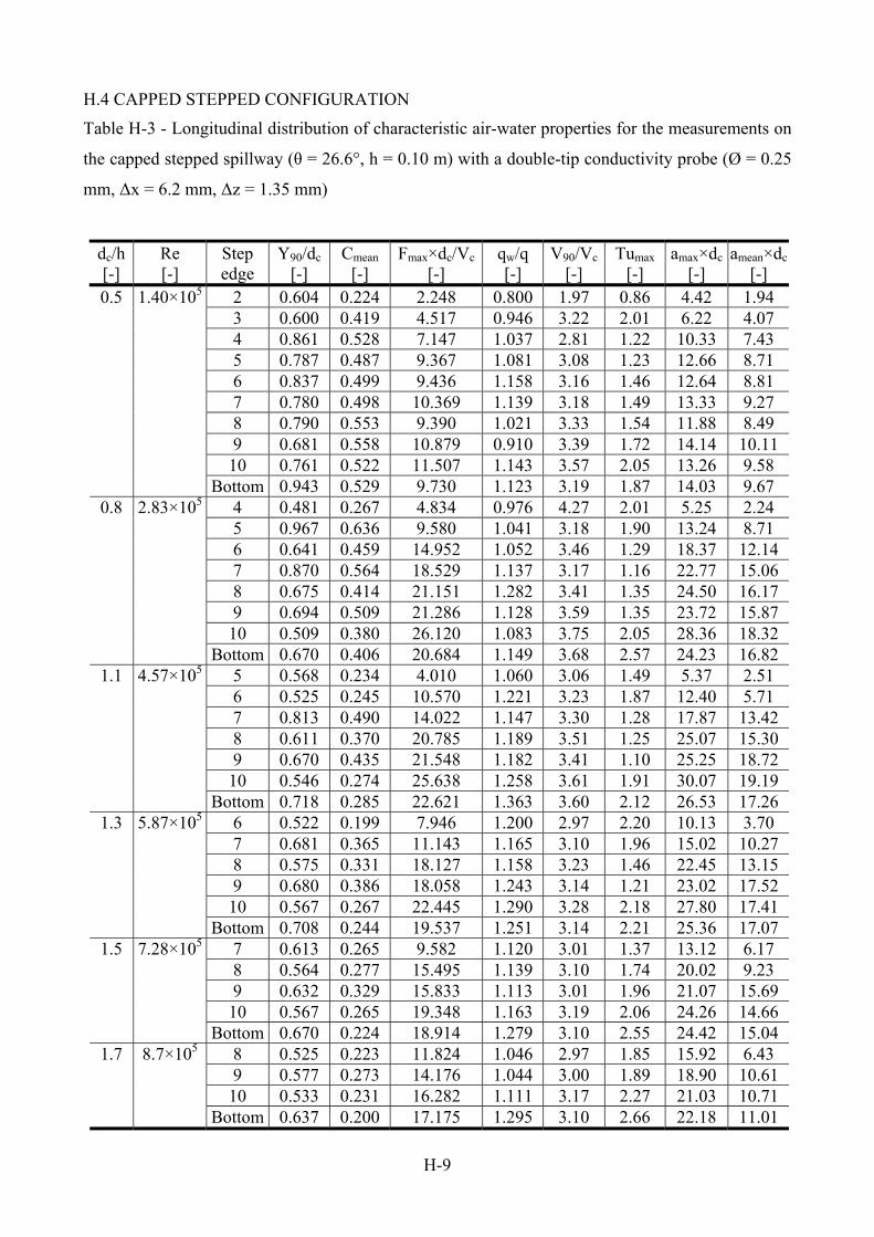
H-9
H.4 CAPPED STEPPED CONFIGURATION
Table H-3 - Longitudinal distribution of characteristic air-water properties for the measurements on
the capped stepped spillway (θ = 26.6°, h = 0.10 m) with a double-tip conductivity probe (Ø = 0.25
mm, Δx = 6.2 mm, Δz = 1.35 mm)
dc/h [-]
Re [-]
Step edge
Y90/dc [-]
Cmean [-]
Fmax×dc/Vc
[-] qw/q
[-] V90/Vc
[-] Tumax
[-] amax×dc
[-] amean×dc
[-] 2 0.604 0.224 2.248 0.800 1.97 0.86 4.42 1.94 3 0.600 0.419 4.517 0.946 3.22 2.01 6.22 4.07 4 0.861 0.528 7.147 1.037 2.81 1.22 10.33 7.43 5 0.787 0.487 9.367 1.081 3.08 1.23 12.66 8.71 6 0.837 0.499 9.436 1.158 3.16 1.46 12.64 8.81 7 0.780 0.498 10.369 1.139 3.18 1.49 13.33 9.27 8 0.790 0.553 9.390 1.021 3.33 1.54 11.88 8.49 9 0.681 0.558 10.879 0.910 3.39 1.72 14.14 10.11 10 0.761 0.522 11.507 1.143 3.57 2.05 13.26 9.58
0.5 1.40×10⁵
Bottom 0.943 0.529 9.730 1.123 3.19 1.87 14.03 9.67 4 0.481 0.267 4.834 0.976 4.27 2.01 5.25 2.24 5 0.967 0.636 9.580 1.041 3.18 1.90 13.24 8.71 6 0.641 0.459 14.952 1.052 3.46 1.29 18.37 12.14 7 0.870 0.564 18.529 1.137 3.17 1.16 22.77 15.06 8 0.675 0.414 21.151 1.282 3.41 1.35 24.50 16.17 9 0.694 0.509 21.286 1.128 3.59 1.35 23.72 15.87 10 0.509 0.380 26.120 1.083 3.75 2.05 28.36 18.32
0.8 2.83×10⁵
Bottom 0.670 0.406 20.684 1.149 3.68 2.57 24.23 16.82 5 0.568 0.234 4.010 1.060 3.06 1.49 5.37 2.51 6 0.525 0.245 10.570 1.221 3.23 1.87 12.40 5.71 7 0.813 0.490 14.022 1.147 3.30 1.28 17.87 13.42 8 0.611 0.370 20.785 1.189 3.51 1.25 25.07 15.30 9 0.670 0.435 21.548 1.182 3.41 1.10 25.25 18.72 10 0.546 0.274 25.638 1.258 3.61 1.91 30.07 19.19
1.1 4.57×10⁵
Bottom 0.718 0.285 22.621 1.363 3.60 2.12 26.53 17.26 6 0.522 0.199 7.946 1.200 2.97 2.20 10.13 3.70 7 0.681 0.365 11.143 1.165 3.10 1.96 15.02 10.27 8 0.575 0.331 18.127 1.158 3.23 1.46 22.45 13.15 9 0.680 0.386 18.058 1.243 3.14 1.21 23.02 17.52 10 0.567 0.267 22.445 1.290 3.28 2.18 27.80 17.41
1.3 5.87×10⁵
Bottom 0.708 0.244 19.537 1.251 3.14 2.21 25.36 17.07 7 0.613 0.265 9.582 1.120 3.01 1.37 13.12 6.17 8 0.564 0.277 15.495 1.139 3.10 1.74 20.02 9.23 9 0.632 0.329 15.833 1.113 3.01 1.96 21.07 15.69 10 0.567 0.265 19.348 1.163 3.19 2.06 24.26 14.66
1.5 7.28×10⁵
Bottom 0.670 0.224 18.914 1.279 3.10 2.55 24.42 15.04 8 0.525 0.223 11.824 1.046 2.97 1.85 15.92 6.43 9 0.577 0.273 14.176 1.044 3.00 1.89 18.90 10.61 10 0.533 0.231 16.282 1.111 3.17 2.27 21.03 10.71
1.7 8.7×10⁵
Bottom 0.637 0.200 17.175 1.295 3.10 2.66 22.18 11.01
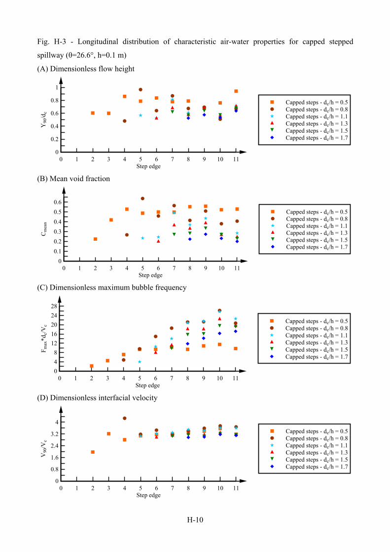
H-10
Fig. H-3 - Longitudinal distribution of characteristic air-water properties for capped stepped
spillway (θ=26.6°, h=0.1 m)
(A) Dimensionless flow height
Step edge
Y90
/dc
0 1 2 3 4 5 6 7 8 9 10 110
0.2
0.4
0.6
0.8
1
Capped steps - dc/h = 0.5Capped steps - dc/h = 0.8Capped steps - dc/h = 1.1Capped steps - dc/h = 1.3Capped steps - dc/h = 1.5Capped steps - dc/h = 1.7
(B) Mean void fraction
Step edge
Cm
ean
0 1 2 3 4 5 6 7 8 9 10 110
0.1
0.2
0.3
0.4
0.5
0.6
Capped steps - dc/h = 0.5Capped steps - dc/h = 0.8Capped steps - dc/h = 1.1Capped steps - dc/h = 1.3Capped steps - dc/h = 1.5Capped steps - dc/h = 1.7
(C) Dimensionless maximum bubble frequency
Step edge
F max
*dc/
Vc
0 1 2 3 4 5 6 7 8 9 10 110
4
8
12
16
20
24
28
Capped steps - dc/h = 0.5Capped steps - dc/h = 0.8Capped steps - dc/h = 1.1Capped steps - dc/h = 1.3Capped steps - dc/h = 1.5Capped steps - dc/h = 1.7
(D) Dimensionless interfacial velocity
Step edge
V90
/Vc
0 1 2 3 4 5 6 7 8 9 10 110
0.8
1.6
2.4
3.2
4
Capped steps - dc/h = 0.5Capped steps - dc/h = 0.8Capped steps - dc/h = 1.1Capped steps - dc/h = 1.3Capped steps - dc/h = 1.5Capped steps - dc/h = 1.7
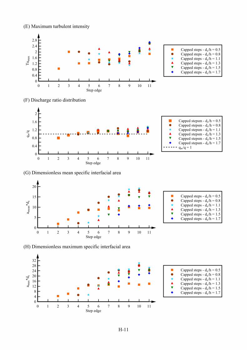
H-11
(E) Maximum turbulent intensity
Step edge
Tu m
ax
0 1 2 3 4 5 6 7 8 9 10 110
0.4
0.8
1.2
1.6
2
2.4
2.8
Capped steps - dc/h = 0.5Capped steps - dc/h = 0.8Capped steps - dc/h = 1.1Capped steps - dc/h = 1.3Capped steps - dc/h = 1.5Capped steps - dc/h = 1.7
(F) Discharge ratio distribution
Step edge
q w/q
0 1 2 3 4 5 6 7 8 9 10 110
0.4
0.8
1.2
1.6
2
Capped stepsm - dc/h = 0.5Capped stepsm - dc/h = 0.8Capped stepsm - dc/h = 1.1Capped stepsm - dc/h = 1.3Capped stepsm - dc/h = 1.5Capped stepsm - dc/h = 1.7qw/q = 1
(G) Dimensionless mean specific interfacial area
Step edge
a mea
n*d c
0 1 2 3 4 5 6 7 8 9 10 110
5
10
15
20
Capped steps - dc/h = 0.5Capped steps - dc/h = 0.8Capped steps - dc/h = 1.1Capped steps - dc/h = 1.3Capped steps - dc/h = 1.5Capped steps - dc/h = 1.7
(H) Dimensionless maximum specific interfacial area
Step edge
a max
*dc
0 1 2 3 4 5 6 7 8 9 10 11048
121620242832
Capped steps - dc/h = 0.5Capped steps - dc/h = 0.8Capped steps - dc/h = 1.1Capped steps - dc/h = 1.3Capped steps - dc/h = 1.5Capped steps - dc/h = 1.7
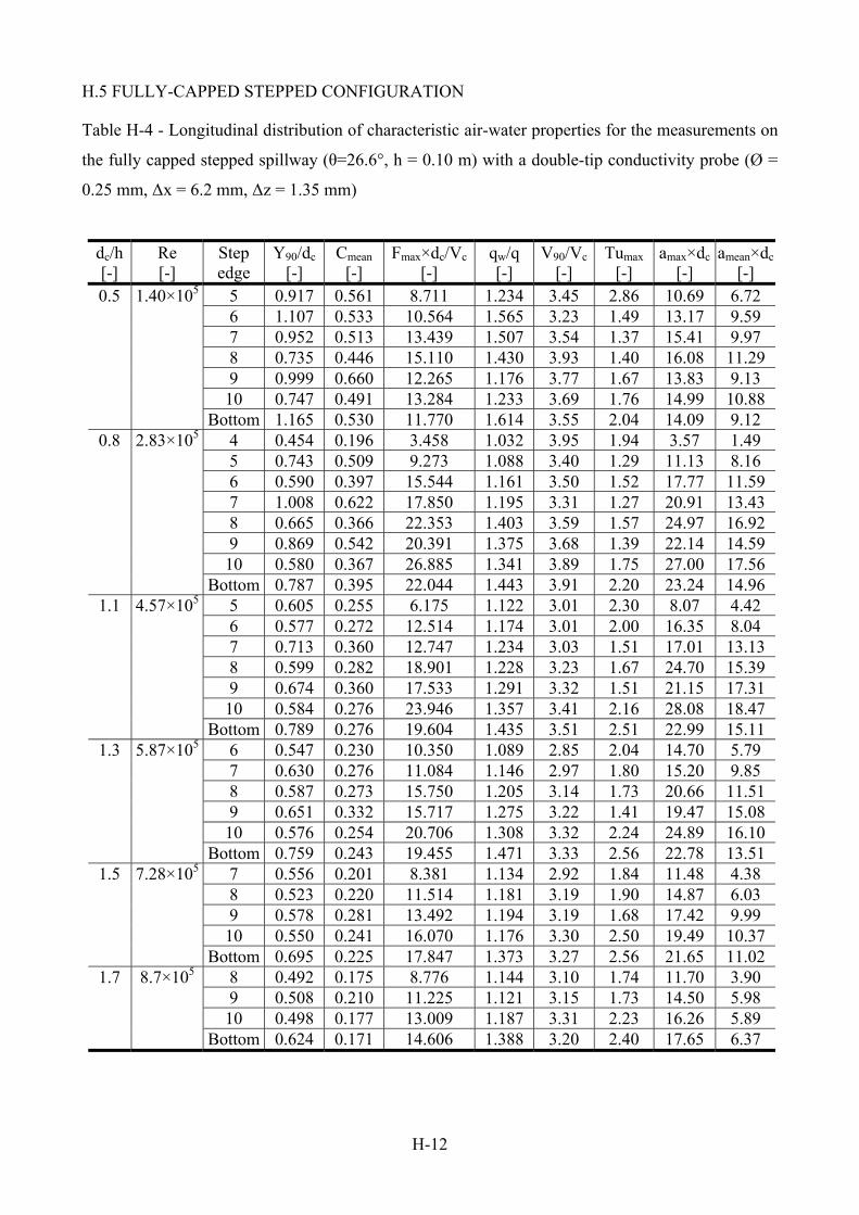
H-12
H.5 FULLY-CAPPED STEPPED CONFIGURATION
Table H-4 - Longitudinal distribution of characteristic air-water properties for the measurements on
the fully capped stepped spillway (θ=26.6°, h = 0.10 m) with a double-tip conductivity probe (Ø =
0.25 mm, Δx = 6.2 mm, Δz = 1.35 mm)
dc/h [-]
Re [-]
Step edge
Y90/dc [-]
Cmean [-]
Fmax×dc/Vc
[-] qw/q
[-] V90/Vc
[-] Tumax
[-] amax×dc
[-] amean×dc
[-] 5 0.917 0.561 8.711 1.234 3.45 2.86 10.69 6.72 6 1.107 0.533 10.564 1.565 3.23 1.49 13.17 9.59 7 0.952 0.513 13.439 1.507 3.54 1.37 15.41 9.97 8 0.735 0.446 15.110 1.430 3.93 1.40 16.08 11.29 9 0.999 0.660 12.265 1.176 3.77 1.67 13.83 9.13 10 0.747 0.491 13.284 1.233 3.69 1.76 14.99 10.88
0.5 1.40×10⁵
Bottom 1.165 0.530 11.770 1.614 3.55 2.04 14.09 9.12 4 0.454 0.196 3.458 1.032 3.95 1.94 3.57 1.49 5 0.743 0.509 9.273 1.088 3.40 1.29 11.13 8.16 6 0.590 0.397 15.544 1.161 3.50 1.52 17.77 11.59 7 1.008 0.622 17.850 1.195 3.31 1.27 20.91 13.43 8 0.665 0.366 22.353 1.403 3.59 1.57 24.97 16.92 9 0.869 0.542 20.391 1.375 3.68 1.39 22.14 14.59 10 0.580 0.367 26.885 1.341 3.89 1.75 27.00 17.56
0.8 2.83×10⁵
Bottom 0.787 0.395 22.044 1.443 3.91 2.20 23.24 14.96 5 0.605 0.255 6.175 1.122 3.01 2.30 8.07 4.42 6 0.577 0.272 12.514 1.174 3.01 2.00 16.35 8.04 7 0.713 0.360 12.747 1.234 3.03 1.51 17.01 13.13 8 0.599 0.282 18.901 1.228 3.23 1.67 24.70 15.39 9 0.674 0.360 17.533 1.291 3.32 1.51 21.15 17.31 10 0.584 0.276 23.946 1.357 3.41 2.16 28.08 18.47
1.1 4.57×10⁵
Bottom 0.789 0.276 19.604 1.435 3.51 2.51 22.99 15.11 6 0.547 0.230 10.350 1.089 2.85 2.04 14.70 5.79 7 0.630 0.276 11.084 1.146 2.97 1.80 15.20 9.85 8 0.587 0.273 15.750 1.205 3.14 1.73 20.66 11.51 9 0.651 0.332 15.717 1.275 3.22 1.41 19.47 15.08 10 0.576 0.254 20.706 1.308 3.32 2.24 24.89 16.10
1.3 5.87×10⁵
Bottom 0.759 0.243 19.455 1.471 3.33 2.56 22.78 13.51 7 0.556 0.201 8.381 1.134 2.92 1.84 11.48 4.38 8 0.523 0.220 11.514 1.181 3.19 1.90 14.87 6.03 9 0.578 0.281 13.492 1.194 3.19 1.68 17.42 9.99 10 0.550 0.241 16.070 1.176 3.30 2.50 19.49 10.37
1.5 7.28×10⁵
Bottom 0.695 0.225 17.847 1.373 3.27 2.56 21.65 11.02 8 0.492 0.175 8.776 1.144 3.10 1.74 11.70 3.90 9 0.508 0.210 11.225 1.121 3.15 1.73 14.50 5.98 10 0.498 0.177 13.009 1.187 3.31 2.23 16.26 5.89
1.7 8.7×10⁵
Bottom 0.624 0.171 14.606 1.388 3.20 2.40 17.65 6.37
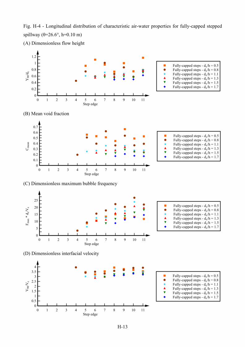
H-13
Fig. H-4 - Longitudinal distribution of characteristic air-water properties for fully-capped stepped
spillway (θ=26.6°, h=0.10 m)
(A) Dimensionless flow height
Step edge
Y90
/dc
0 1 2 3 4 5 6 7 8 9 10 110
0.2
0.4
0.6
0.8
1
1.2
Fully-capped steps - dc/h = 0.5Fully-capped steps - dc/h = 0.8Fully-capped steps - dc/h = 1.1Fully-capped steps - dc/h = 1.3Fully-capped steps - dc/h = 1.5Fully-capped steps - dc/h = 1.7
(B) Mean void fraction
Step edge
Cm
ean
0 1 2 3 4 5 6 7 8 9 10 110
0.1
0.2
0.3
0.4
0.5
0.6
0.7
Fully-capped steps - dc/h = 0.5Fully-capped steps - dc/h = 0.8Fully-capped steps - dc/h = 1.1Fully-capped steps - dc/h = 1.3Fully-capped steps - dc/h = 1.5Fully-capped steps - dc/h = 1.7
(C) Dimensionless maximum bubble frequency
Step edge
F max
* d
c/V
c
0 1 2 3 4 5 6 7 8 9 10 110
5
10
15
20
25
Fully-capped steps - dc/h = 0.5Fully-capped steps - dc/h = 0.8Fully-capped steps - dc/h = 1.1Fully-capped steps - dc/h = 1.3Fully-capped steps - dc/h = 1.5Fully-capped steps - dc/h = 1.7
(D) Dimensionless interfacial velocity
Step edge
V90
/Vc
0 1 2 3 4 5 6 7 8 9 10 110
0.51
1.52
2.53
3.54
Fully-capped steps - dc/h = 0.5Fully-capped steps - dc/h = 0.8Fully-capped steps - dc/h = 1.1Fully-capped steps - dc/h = 1.3Fully-capped steps - dc/h = 1.5Fully-capped steps - dc/h = 1.7
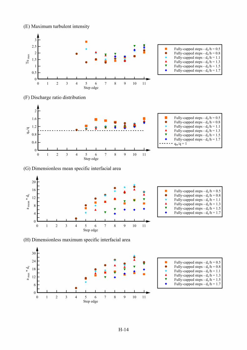
H-14
(E) Maximum turbulent intensity
Step edge
Tu
max
0 1 2 3 4 5 6 7 8 9 10 110
0.5
1
1.5
2
2.5
3
Fully-capped steps - dc/h = 0.5Fully-capped steps - dc/h = 0.8Fully-capped steps - dc/h = 1.1Fully-capped steps - dc/h = 1.3Fully-capped steps - dc/h = 1.5Fully-capped steps - dc/h = 1.7
(F) Discharge ratio distribution
Step edge
q w/q
0 1 2 3 4 5 6 7 8 9 10 110
0.4
0.8
1.2
1.6
2
Fully-capped steps - dc/h = 0.5Fully-capped steps - dc/h = 0.8Fully-capped steps - dc/h = 1.1Fully-capped steps - dc/h = 1.3Fully-capped steps - dc/h = 1.5Fully-capped steps - dc/h = 1.7qw/q = 1
(G) Dimensionless mean specific interfacial area
Step edge
a m
ean
* d c
0 1 2 3 4 5 6 7 8 9 10 110
4
8
12
16
20
Fully-capped steps - dc/h = 0.5Fully-capped steps - dc/h = 0.8Fully-capped steps - dc/h = 1.1Fully-capped steps - dc/h = 1.3Fully-capped steps - dc/h = 1.5Fully-capped steps - dc/h = 1.7
(H) Dimensionless maximum specific interfacial area
Step edge
a m
ax *
dc
0 1 2 3 4 5 6 7 8 9 10 110
6
12
18
24
30
Fully-capped steps - dc/h = 0.5Fully-capped steps - dc/h = 0.8Fully-capped steps - dc/h = 1.1Fully-capped steps - dc/h = 1.3Fully-capped steps - dc/h = 1.5Fully-capped steps - dc/h = 1.7
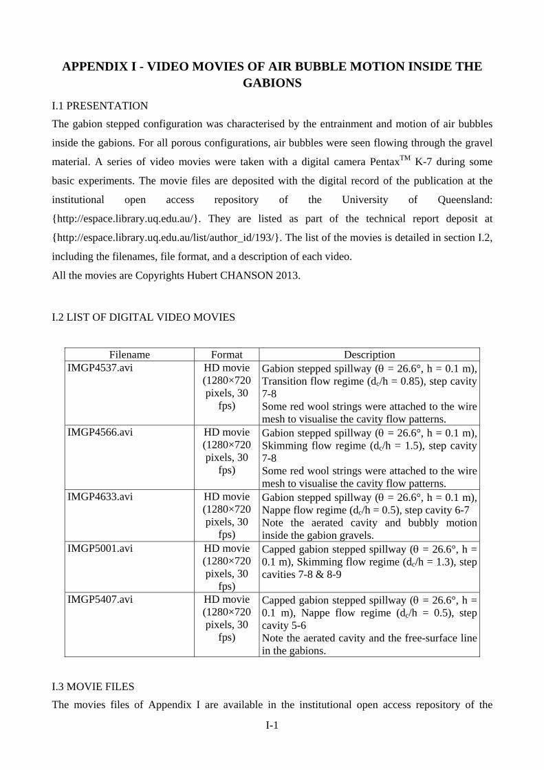
I-1
APPENDIX I - VIDEO MOVIES OF AIR BUBBLE MOTION INSIDE THE GABIONS
I.1 PRESENTATION
The gabion stepped configuration was characterised by the entrainment and motion of air bubbles
inside the gabions. For all porous configurations, air bubbles were seen flowing through the gravel
material. A series of video movies were taken with a digital camera PentaxTM K-7 during some
basic experiments. The movie files are deposited with the digital record of the publication at the
institutional open access repository of the University of Queensland:
{http://espace.library.uq.edu.au/}. They are listed as part of the technical report deposit at
{http://espace.library.uq.edu.au/list/author_id/193/}. The list of the movies is detailed in section I.2,
including the filenames, file format, and a description of each video.
All the movies are Copyrights Hubert CHANSON 2013.
I.2 LIST OF DIGITAL VIDEO MOVIES
Filename Format Description IMGP4537.avi HD movie
(1280×720 pixels, 30
fps)
Gabion stepped spillway ( = 26.6°, h = 0.1 m), Transition flow regime (dc/h = 0.85), step cavity 7-8 Some red wool strings were attached to the wire mesh to visualise the cavity flow patterns.
IMGP4566.avi HD movie (1280×720 pixels, 30
fps)
Gabion stepped spillway ( = 26.6°, h = 0.1 m), Skimming flow regime (dc/h = 1.5), step cavity 7-8 Some red wool strings were attached to the wire mesh to visualise the cavity flow patterns.
IMGP4633.avi HD movie (1280×720 pixels, 30
fps)
Gabion stepped spillway ( = 26.6°, h = 0.1 m), Nappe flow regime (dc/h = 0.5), step cavity 6-7 Note the aerated cavity and bubbly motion inside the gabion gravels.
IMGP5001.avi HD movie (1280×720 pixels, 30
fps)
Capped gabion stepped spillway ( = 26.6°, h = 0.1 m), Skimming flow regime (dc/h = 1.3), step cavities 7-8 & 8-9
IMGP5407.avi HD movie (1280×720 pixels, 30
fps)
Capped gabion stepped spillway ( = 26.6°, h = 0.1 m), Nappe flow regime (dc/h = 0.5), step cavity 5-6 Note the aerated cavity and the free-surface line in the gabions.
I.3 MOVIE FILES
The movies files of Appendix I are available in the institutional open access repository of the
I-2
University of Queensland (Brisbane, Australia) and they are deposited at UQeSpace
{http://espace.library.uq.edu.au/}. The digital video files are a series of HD movies. The deposited
movie files (Section I.2) were converted to Flash video for video streaming. At request, the second
author might provide the original movies as a single compressed file.
The copyrights of the movies remain the property of Hubert CHANSON. Any use of the movies
available in the digital appendix must acknowledge and cite the present report:
WUTHRICH, D., and CHANSON, H. (2014). "Aeration and Energy Dissipation over Stepped
Gabion Spillways: a Physical Study." Hydraulic Model Report No. CH92/13, School of Civil
Engineering, The University of Queensland, Brisbane, Australia, 171 pages & 5 video movies
(ISBN 9781742720944).
Further details on the report including the digital appendix may be obtained from Professor Hubert
CHANSON {[email protected]}.
R-1
REFERENCES
AGOSTINI, R., BIZZARRI, A., MASETTI, M., and PAPETTI, A. (1987). "Flexible Gabion and
Reno Mattress Structures in River and Stream Training Works. Section One : Weirs." Officine
Maccaferri, Bologna, Italy, 2nd edition.
ANDRE, S., BOILLAT, J.L., SCHLEISS, A.J., and MATOS, J. (2004). "Energy Dissipation and
Hydrodynamic Forces of Aerated Flow over Macro-Roughness Linings for Overtopped
Embankment Dams." Proc. Intl Conf. on Hydraulics of Dams and River Structures, Tehran, Iran,
Balkema Publ., The Netherlands, pp. 189-196.
BOES, R.M. (2000). "Zweiphasenstroömung und Energieumsetzung an Grosskaskaden." ('Two-
Phase Flow and Energy Dissipation on Cascades.') Ph.D. thesis, VAW-ETH, Zürich,
Switzerland, 166 pages (in German).
BUNG, D.B., and SCHLENKHOFF, A. (2010). "Self-aerated Flow on Embankment Stepped
Spillways - The Effect of Additional Micro-roughness on Energy Dissipation and Oxygen
Transfer." Proc. 1st IAHR European Congress, 4-6 May, Edinburgh, Scotland, 6 pages (CD-
ROM).
CAIN, P., and WOOD, I.R. (1981). "Instrumentation for Aerated Flow on Spillways." Jl of Hyd.
Div., ASCE, Vol. 107, HY11, Nov., pp. 1407-1424.
CAROSI, G. and CHANSON, H. (2008). "Turbulence Characteristics in Skimming Flows on
Stepped Spillways." Canadian Journal of Civil Engineering, Vol. 35, No. 9, pp. 865-880.
CHAMANI, M.R., and RAJARATNAM, N. (1994). "Jet Flow on Stepped Spillways." Jl of Hyd.
Engrg., ASCE, Vol. 120, No. 2, pp. 254-259.
CHANSON, H. (1994a). "Hydraulics of Nappe Flow Regime above Stepped Chutes and
Spillways." Australian Civil Engineering Transactions, Institution of Engineers, Australia, Vol.
CE36, No. 1, Jan., pp. 69-76.
CHANSON, H. (1994b). "Hydraulics of Skimming Flows over Stepped Channels and Spillways."
Journal of Hydraulic Research, IAHR, Vol. 32, No. 3, pp. 445-460.
CHANSON, H. (1995a). "Hydraulic Design of Stepped Cascades, Channels, Weirs and Spillways."
Pergamon, Oxford, UK, 292 pages.
CHANSON, H. (1995b). "Air Bubble Entrainment in Free-surface Turbulent Flows. Experimental
Investigations." Hydraulic Model Report CH46/95, Dept. of Civil Engineering, University of
Queensland, Australia, June, 368 pages.
CHANSON, H. (1997). "Air Bubble Entrainment in Open Channels. Flow Structure and Bubble
Size Distributions." International Journal of Multiphase Flow, Vol. 23, No. 1, pp. 193-203.
CHANSON, H. (2000). "Forum article. Hydraulics of Stepped Spillways: Current Status", Jl of
Hyd. Engrg., ASCE, Vol. 126, No. 9, pp. 636-637.
CHANSON, H. (2000-2001). "Historical Development of Stepped Cascades for the Dissipation of
Hydraulic Energy." Transactions of the Newcomen Society, Vol. 71, No. 2, pp. 295-318.
CHANSON, H. (2001). "The Hydraulics of Stepped Chutes and Spillways." Balkema, Lisse, The
Netherlands, 384 pages.
R-2
CHANSON, H. (2002). "Air-Water Flow Measurements with Intrusive Phase-Detection Probes.
Can we Improve their Interpretation ?." Jl of Hyd. Engrg., ASCE, Vol. 128, No. 3, pp. 252-255.
CHANSON, H. (2006). "Hydraulics of Skimming Flows on Stepped Chutes: the Effects of Inflow
Conditions?" Journal of Hydraulic Research, IAHR, Vol. 44, No. 1, pp. 51-60.
CHANSON, H. (2009). "Turbulent Air-water Flows in Hydraulic Structures: Dynamic Similarity
and Scale Effects." Environmental Fluid Mechanics, Vol. 9, No. 2, pp. 125-142 (DOI:
10.1007/s10652-008-9078-3).
CHANSON, H. (2013). "Hydraulics of Aerated Flows: Qui Pro Quo?" Journal of Hydraulic
Research, IAHR, Invited Vision paper, Vol. 51, No. 3, pp. 223-243 (DOI:
10.1080/00221686.2013.795917).
CHANSON, H., and CAROSI, G. (2007). "Advanced Post-Processing and Correlation Analyses in
High-Velocity Air-Water Flows." Environmental Fluid Mechanics, Vol. 7, No. 6, pp. 495-508
(DOI 10.1007/s10652-007-9038-3).
CHANSON, H. and FELDER, S. (2010). "Turbulence Measurements in Air-water self-aerated
Flows: Basic Analysis and Results." 7th international conference on Multiphase Flow, ICMF
2010, Tampa FL, USA, 30 May - 5 June 2010, pp. 1-11.
CHANSON, H., and GONZALEZ, C.A. (2005). "Physical Modelling and Scale Effects of Air-
Water Flows on Stepped Spillways." Journal of Zhejiang University SCIENCE, Vol. 6A, No. 3,
March, pp. 243-250.
CHANSON, H. and TOOMBES, L. (2002a). "Energy Dissipation and Air Entrainment in Stepped
Storm Waterway: Experimental Study." Journal of Irrigation and Drainage Engineering, Vol.
128, No. 5, pp. 305-315.
CHANSON, H. and TOOMBES, L. (2002b). "Air-Water Flows down Stepped chutes: Turbulence
and Flow Structure Observations." International Journal of Multiphase Flow, Vol. 28, No. 11,
pp. 1737-1761.
CHANSON, H. and TOOMBES, L. (2002c). "Experimental Study of Gas-Liquid Interfacial
Properties in a Stepped Cascade Flow." Environmental Fluid Mechanics, Vol. 2, No. 3, pp. 241-
263.
CHANSON, H. and TOOMBES, L. (2004). "Hydraulics of stepped chutes: The transition flow."
Journal of Hydraulic Research, Vol. 42, No. 1, pp. 43-54.
CHANSON, H., YASUDA, Y. and OHTSU, I. (2002). "Flow Resistance in Skimming Flows and
its Modelling." Canadian Journal of Civil Engineering, Vol. 29, No. 6, pp. 809-819.
CORSI, R., MADANI-ISFAHANI, M. and ZYTNER, R. (1992). "Oxygen Transfer and VOC
Emissions from Sewer Drop Structures." Water Environment Research, No. 69, Vol. 3, pp. 286-
294.
CROWE, C., SOMMERFIELD, M., and TSUJI, Y. (1998). "Multiphase Flows with Droplets and
Particles." CRC Press, Boca Raton, USA, 471 pages.
DARCY, H. (1856). "Les Fontaines Publiques de la Ville de Dijon." Dalmont, Paris.
R-3
FELDER, S. (2013). "Air-water flow properties on stepped spillways for embankment dams:
Aeration, energy dissipation and turbulence on uniform, non-uniform and pooled stepped
chutes." PhD Thesis, School of Civil Engineering, The University of Queensland, 506 pages.
FELDER, S., and CHANSON, H. (2009). "Energy dissipation, flow resistance and gas-liquid
interfacial area in skimming flows on moderate-slope stepped spillways." Environmental Fluid
Mechanics, Vol. 9, No. 4, pp. 427-441.
FELDER, S. and CHANSON, H. (2011). "Energy Dissipation down a Stepped Spillway with Non-
Uniform Step Heights". Journal of Hydraulic Engineering, Vol. 137, No. 11, pp. 1543-1548.
FELDER, S. and CHANSON, H. (2012). "Free-surface Profiles, Velocity and Pressure
Distributions on a Broad-Crested Weir: a Physical study." Journal of Irrigation and Drainage
Engineering, Vol. 138, No. 12, pp. 1068–1074.
FELDER, S., and CHANSON, H. (2013a). "Air–water Flow Measurements in a Flat Slope Pooled
Stepped Waterway." Canadian Journal of Civil Engineering, Vol. 40, No. 4, pp. 361-372 (DOI:
10.1139/cjce-2012-0464).
FELDER, S. and CHANSON, H. (2013b). "Air Entrainment and Energy Dissipation on Porous
Pooled Stepped Spillways." Proceedings of International Workshop on Hydraulic Design of
Low-Head Structures, Aachen, Germany, D.BUNG and S.PAGLIARA Editors, pp. 87-97.
FELDER, S., and CHANSON, H. (2014). "Triple Decomposition Technique in Air–Water Flows:
Application to Instationary Flows on a Stepped Spillway." International Journal of Multiphase
Flow, Vol. 58, pp. 139-153 & 3 videos (DOI: 10.1016/j.ijmultiphaseflow.2013.09.006).
FERRELL, R.T. and HIMMELBLAU, D.M. (1967). "Diffusion Coefficients of Nitrogen and
Oxygen in Water." Journal of Chemical Engineering Data, Vol. 12, No. 1, pp. 111-115.
GASPAROTTO, R. (1992). "Waterfall Aeration Works." Civil Engineering, ASCE, Vol. 62, No.
10, pp. 52-54.
GONZALEZ, C. (2005). "Experimental Study of Free-surface Aeration on Embankment Stepped
Chutes." Ph.D. Thesis, The University of Queensland, Department of Civil Engineering,
Brisbane, Australia, 240 pages.
GONZALEZ, C.A., and CHANSON, H. (2004). "Interactions between Cavity Flow and Main
Stream Skimming Flows: an Experimental Study." Canadian Journal of Civil Engineering, Vol.
31, No. 1, pp. 33-44.
GONZALEZ, C. and CHANSON, H. (2008). "Turbulence and cavity recirculation in air-water
skimming flows on a stepped spillway." Journal of Hydraulic Research, Vol. 46, No. 1, pp. 65-
72.
GONZALEZ, C., MASAYUKI, T., and CHANSON, H. (2008). "An experimental study of effects
of step roughness in skimming flows on stepped chutes." Journal of Hydraulic Research, Vol.
46, No. 1, pp. 24-35.
GOSSE, P., and GREGOIRE, A. (1997). "Dispositif de Réoxygénation Artificielle du Sinnamary à
l'Aval du Barrage de Petit-Saut (Guyane)." ('Artificial Re-Oxygenation of the Sinnamary,
Downstream of Petit-Saut Dam (French Guyana).') Hydroécol. Appl., Tome 9, No. 1-2, pp. 23-
56 (in French).

R-4
HAUSER, G.E., SHANE, R.M., NIZNIK, J.A., and BROCK, W.G. (1992). "Innovative
Reregulation Weirs." Civil Engineering, ASCE, Vol. 62, No. 5, pp. 64-66.
GUENTHER, P., FELDER, S., and CHANSON, H. (2013). "Flow Aeration, Cavity Processes and
Energy Dissipation on Flat and Pooled Stepped Spillways for Embankments." Environmental
Fluid Mechanics, Vol. 13, No. 5, pp. 503-525 (DOI: 10.1007/s10652-013-9277-4).
GULLIVER, J.S. (1990) "Introduction to Air-Water Mass Transfer." Proc. 2nd Intl Symp on Gas
Transfer at Water Surfaces, Air-Water Mass Transfer, ASCE Publ., S.C. WILHELMS and J.S.
GULLIVER Editors, Minneapolis MN, USA, pp. 1-7.
HERRINGE, R.A. and DAVIS, M.R. (1974). "Detection of instantaneous Phase Changes in Gas-
Liquid Mixtures." Journal of Physics E: Scientific Instruments, Vol. 7, pp. 807-812.
HORTON, N.A. AND POKRAJAC, D. (2009). "Onset of turbulence in a regular porous medium:
An experimental study." Physics of Fluids, Vol. 21, No. 4, 045104, 13 pages.
JOY, D.M. (1991), "Non-linear flow in a coarse porous media." Proceedings of the 10th Canadian
Hydrotechnical Conference, CSCE, Vol. 1, Vancouver, BC. May29-31, pp. 106.115.
KAWASE, Y. and MOO-YOUNG, M. (1992) "Correlations for Liquid-Phase Mass Transfer
Coefficients in Bubble Column Reactors with Newtonian and Non-Newtonian Fluids." Canadian
Journal of Chemical Engineering, Vol. 70, Feb, pp. 48-54.
KELLS, J.A. (1993). "Spatially varied flow over rockfill embankments." Canadian Journal of Civil
Engineering, Vol. 20, pp. 820-827.
KELLS, J.A. (1995). "Comparison of Energy Dissipation between Nappe and Skimming Flow
Regimes on Stepped Chutes - Discussion." Jl of Hyd. Res., IAHR, Vol. 33, No. 1, pp. 128-133.
KÖKPINAR, M. (2004). "Flow over a Stepped Chute with and without Macro-Roughness
Elements." Canadian Journal of Civil Engineering, Vol. 31, No. 5, pp. 880-891.
KRAHN, J., FREDLUND, D.G., LAM, L. AND BARBOUR, S.L. (1987). "PC-SEEP a finite
element program for modelling seepage." First Canadian Symposium on Microcomputer
application to Geotechnique, Regina, Sak., October 22-23, pp. 243-251.
MINOR, H.E., and HAGER, W.H. (2000). "Hydraulics of Stepped Spillways." Intl Workshop on
Hydraulics of Stepped Spillways, Zürich, Switzerland, Balkema Publ., Lisse, The Netherlands.
OHTSU, I., and YASUDA, Y. (1998). "Hydraulic Characteristics of Stepped Channel Flows."
Workshop on Flow Characteristics around Hydraulic Structures and River Environment,
University Research Center, Nihon University, Tokyo, Japan, 55 pages.
OHTSU, I., YASUDA, Y., and TAKAHASHI, M. (2004). "Flow Characteristics of Skimming
Flows in Stepped Channels." Jl of Hyd. Engrg., ASCE, Vol. 130, No. 9, pp. 860-869.
Discussion: Vol. 132, No. 5, pp. 527-542.
NAKASONE, H. (1987). "Study of Aeration at Weirs and Cascades." Jl of Envir. Engrg., ASCE,
Vol. 113, No. 1, pp. 64-81.
PEYRAS, L., ROYET, P., and DEGOUTTE, G. (1991). "Ecoulement et Dissipation sur les
Déversoirs en Gradins de Gabions." ('Flows and Dissipation of Energy on Gabion Weirs.') Jl La
Houille Blanche, No. 1, pp. 37-47 (in French).
R-5
PEYRAS, L., ROYET, P. and DEGOUTTE, G. (1992). "Flow and energy dissipation over stepped
gabion weirs." Journal of Hydraulic Engineering, Vol. 118, No. 5, pp. 707-717.
PFISTER, M., and CHANSON, H. (2012). "Scale Effects in Physical Hydraulic Engineering
Models. Discussion." Journal of Hydraulic Research, IAHR, Vol. 50, No. 2, pp. 244-246 (DOI
10.1080/00221686.2012.654672).
RAJARATNAM, N. (1990). "Skimming Flow in Stepped Spillways." Journal of Hydraulic
Engineering, ASCE, Vol. 116, No. 4, pp. 587-591.
RAUDKIVI, A.J., and CALLANDER, R.A. (1976). "Analysis of Groundwater Flow." Edward
Arnold Publisher, London, UK.
STEPHENSON, D. (1979). "Gabion Energy Dissipators." Proc. 13th ICOLD Congress, New Delhi,
India, Q. 50, R. 3, pp. 33-43.
TOOMBES, L. (2002). "Experimental Study of Air-Water Flow Properties on Low-Gradient
Stepped Cascades." Ph.D. Thesis, University of Queensland, School of Civil Engineering,
Brisbane, Australia, 304 pages.
TOOMBES, L. and CHANSON, H. (2005). "Air-water mass transfer on a stepped spillway."
Journal of Environmental Engineering, Vol. 131, No. 10, pp. 1377-1386.
TOOMBES, L. and CHANSON, H. (2008a). "Flow Patterns in Nappe Flow Regime down Low
Gradient Stepped Chutes." Journal of Hydraulic Research, Vol. 46, No. 1, pp. 4-14.
TOOMBES, L. and CHANSON, H. (2008b). "Interfacial Aeration and Bubble Count Rate
Distributions in a Supercritical Flow Past a Backward-Facing Step." International Journal of
Multiphase Flow, Vol. 34, No. 5, pp. 427-436.
WOOD, I.R. (1991). "Air Entrainment in Free-Surface Flows." IAHR Hydraulic Structures Design
Manual No. 4, Hydraulic Design Considerations, Balkema Publ., Rotterdam, The Netherlands,
149 pages.
Bibliography
ANDRE, S. (2004). "High Velocity Aerated Flows on Stepped Chutes with Macro-Roughness
Elements." Ph.D. thesis, Ecole Polytechnique Fédérale de Lausanne EPFL-LCH, Lausanne,
Switzerland, 272 pages.
ANDRE, S., BOILLAT, J.L., and SCHLEISS, A. (2005). "Two-Phase Flow Characteristics of
Stepped Spillways. Discussion" Jl of Hyd. Engrg., ASCE, Vol. 131, No. 5, pp. 423-427.
BUNG, D. B. (2009). "Zur selbstbelüfteten Gerinneströmung auf Kaskaden mit gemäßigter
Neigung." Ph.D. thesis, Bergische University of Wuppertal, Germany, 292 pages (in German).
CHAMANI, M.R., and RAJARATNAM, N. (1999). "Characteristics of Skimming Flow over
Stepped Spillways." Jl of Hyd. Engrg., ASCE, Vol. 125, No. 4, pp. 361-368. Discussion : Vol.
126, No. 11, pp. 860-872. Closure : Vol. 126, No. 11, pp. 872-873.
R-6
CHAMANI, M.R., and RAJARATNAM, N. (1999). "Onset of Skimming Flow on Stepped
Spillways." Jl of Hyd. Engrg., ASCE, Vol. 125, No. 9, pp. 969-971. Discussion : Vol. 127, No.
6, pp. 519-525.
CHANSON, H. (1994). "Hydraulics of Skimming Flows over Stepped Channels and Spillways." Jl
of Hyd. Res., IAHR, Vol. 32, No. 3, pp. 445-460. Discussion : Vol. 33, No. 3, pp. 414-419 (ISSN
0022-1686).
CHANSON, H. (1994). "Comparison of Energy Dissipation between Nappe and Skimming Flow
Regimes on Stepped Chutes." Jl of Hyd. Res., IAHR, Vol. 32, No. 2, pp. 213-218. Errata : Vol.
33, No. 1, p. 113. Discussion : Vol. 33, No. 1, pp. 114-143 (ISSN 0022-1686).
FELDER, S. and CHANSON, H. (2012). "Air-Water Flow Measurements in Instationary Free-
Surface Flows: a Triple Decomposition Technique." Hydraulic Model Report CH85/12, School
of Civil Engineering, The University of Queensland, Brisbane, Australia, 161 pages.
FELDER, S., and CHANSON, H. (2013). "Aeration, Flow Instabilities, and Residual Energy on
Pooled Stepped Spillways of Embankment Dams." Journal of Irrigation and Drainage
Engineering, ASCE, Vol. 139, No. 10, pp. 880-887 (DOI: 10.1061/(ASCE)IR.1943-
4774.0000627) (ISSN 0733-9437).
FELDER, S., FROMM, C. and CHANSON, H. (2012). "Air Entrainment and Energy Dissipation
on a 8.9° Slope Stepped Spillway with Flat and Pooled Steps." Hydraulic Model Report
CH86/12, University of Queensland, School of Civil Engineering, Brisbane, Australia, 73 pages.
FELDER, S., GUENTHER, P. and CHANSON, H. (2012). "Air-Water Flow Properties and Energy
Dissipation on Stepped Spillways: a Physical Study of Several Pooled Stepped Configurations."
Hydraulic Model Report CH87/12, University of Queensland, School of Civil Engineering,
Brisbane, Australia, 86 pages.
KNAUSS, J. (1995). "ΤΗΣ ΓΡΙΑΣ ΤΟ ΠΗΔΗΜΑ, der Altweibersprung. Die Rätselhafte Alte Talsperre
in der Glosses-Schlucht bei Alyzeia in Akarnanien." Archäologischer Anzeiger, Vol. 5, pp. 138-162.
MEIRELES, I., and MATOS, J. (2009). "Skimming Flow in the Nonaerated Region of Stepped
Spillways over Embankment Dams." Journal of Hydraulic Engineering, Vol. 135, No. 8, pp.
685-689.
SCHLENKHOFF, A., and BUNG, D.B. (2009). "Prediction of Oxygen Transfer in Self-aerated
Skimming Flow on Embankment Stepped Spillways." Proc. 33rd IAHR Biennial Congress,
IAHR-ASCE-EWRI, Vancouver, Canada, 9-14 Aug., 8 pages (CD-ROM).
STEPHENSON, D. (1980). "The Stability of Gabion Weirs." Intl Water Power and Dam
Construction, Vol. 32, No. 4, pp. 24-28.
THORWARTH, J. (2008). Hydraulisches Verhalten der Treppengerinne mit eingetieften Stufen –
Selbstinduzierte Abflussinstationaritäten und Energiedissipation (Hydraulics of Pooled Stepped
Spillways – Self-induced Unsteady Flow and Energy Dissipation). Ph.D. Thesis, University of
Aachen, Aachen, Germany, 239 pages (in German).
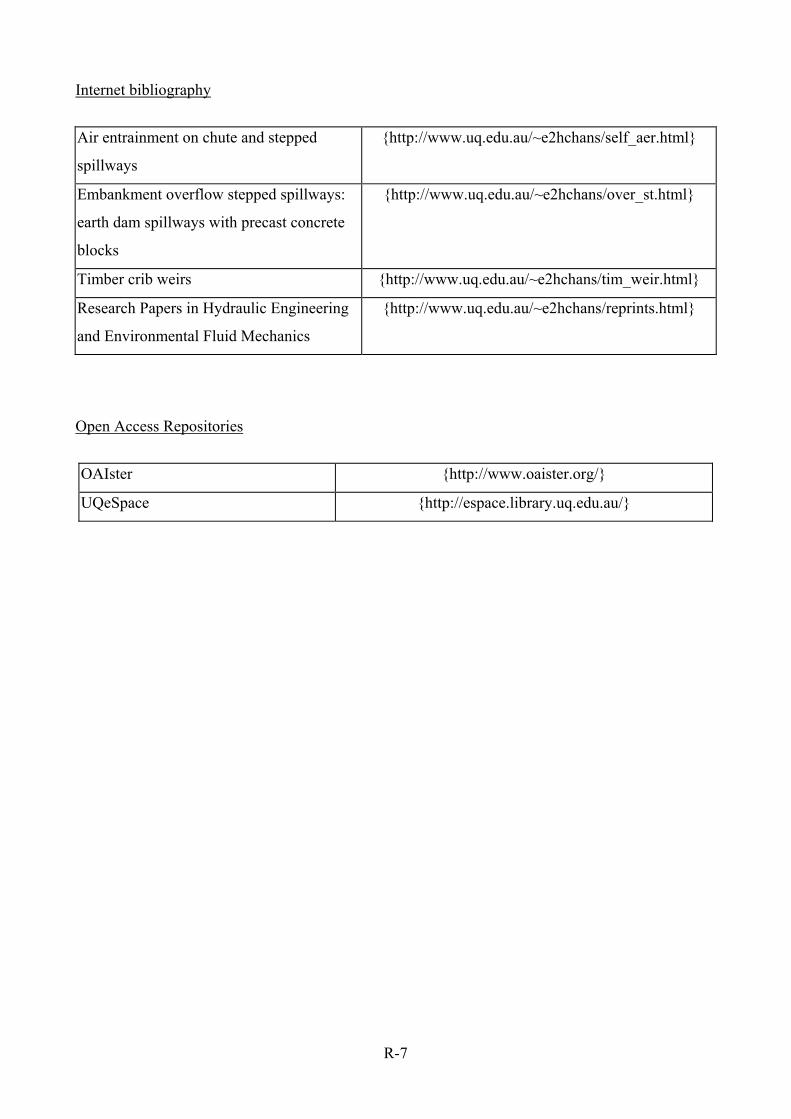
R-7
Internet bibliography
Air entrainment on chute and stepped
spillways
{http://www.uq.edu.au/~e2hchans/self_aer.html}
Embankment overflow stepped spillways:
earth dam spillways with precast concrete
blocks
{http://www.uq.edu.au/~e2hchans/over_st.html}
Timber crib weirs {http://www.uq.edu.au/~e2hchans/tim_weir.html}
Research Papers in Hydraulic Engineering
and Environmental Fluid Mechanics
{http://www.uq.edu.au/~e2hchans/reprints.html}
Open Access Repositories
OAIster {http://www.oaister.org/}
UQeSpace {http://espace.library.uq.edu.au/}
R-8
Bibliographic reference of the Report CH92/13 The Hydraulic Model research report series CH is a refereed publication published by the School of
Civil Engineering at the University of Queensland, Brisbane, Australia.
The bibliographic reference of the present report is:
WUTHRICH, D., and CHANSON, H. (2014). "Aeration and Energy Dissipation over Stepped
Gabion Spillways: a Physical Study." Hydraulic Model Report No. CH92/13, School of Civil
Engineering, The University of Queensland, Brisbane, Australia, 171 pages and 5 video movies
(ISBN 9781742720944).
The Report CH92/13 is available, in the present form, as a PDF file on the Internet at UQeSpace:
http://espace.library.uq.edu.au/
It is listed at:
http://espace.library.uq.edu.au/list/author_id/193/
R-9
HYDRAULIC MODEL RESEARCH REPORT CH
The Hydraulic Model Report CH series is published by the School of Civil Engineering at the
University of Queensland. Orders of any reprint(s) of the Hydraulic Model Reports should be
addressed to the School Secretary.
School Secretary, School of Civil Engineering, The University of Queensland
Brisbane 4072, Australia - Tel.: (61 7) 3365 3619 - Fax : (61 7) 3365 4599
Url: http://www.eng.uq.edu.au/civil/ Email: [email protected]
Report CH Unit price Quantity Total price
WUTHRICH, D., and CHANSON, H. (2014). "Aeration and Energy Dissipation over Stepped Gabion Spillways: a Physical Study." Hydraulic Model Report No. CH92/13, School of Civil Engineering, The University of Queensland, Brisbane, Australia, 171 pages and 5 video movies (ISBN 9781742720944).
AUD$60.00
WANG, H., and CHANSON, H. (2013). "Free-Surface Deformation and Two-Phase Flow Measurements in Hydraulic Jumps". Hydraulic Model Report No. CH91/13, School of Civil Engineering, The University of Queensland, Brisbane, Australia, 108 pages (ISBN 9781742720746).
AUD$60.00
SIMON, B., and CHANSON, H. (2013). "Turbulence Measurements in Tidal Bore-like Positive Surges over a Rough Bed". Hydraulic Model Report No. CH90/12, School of Civil Engineering, The University of Queensland, Brisbane, Australia, 176 pages (ISBN 9781742720685).
AUD$60.00
REUNGOAT, D., CHANSON, H., and CAPLAIN, B. (2012). "Field Measurements in the Tidal Bore of the Garonne River at Arcins (June 2012)." Hydraulic Model Report No. CH89/12, School of Civil Engineering, The University of Queensland, Brisbane, Australia, 121 pages (ISBN 9781742720616).
AUD$60.00
CHANSON, H., and WANG, H. (2012). "Unsteady Discharge Calibration of a Large V-Notch Weir." Hydraulic Model Report No. CH88/12, School of Civil Engineering, The University of Queensland, Brisbane, Australia, 50 pages and 4 movies (ISBN 9781742720579).
AUD$60.00
FELDER, S., FROMM, C., and CHANSON, H. (2012). "Air Entrainment and Energy Dissipation on a 8.9° Slope Stepped Spillway with Flat and Pooled Steps." Hydraulic Model Report No. CH86/12, School of Civil Engineering, The University of Queensland, Brisbane, Australia, 80 pages (ISBN 9781742720531).
AUD$60.00
FELDER, S., and CHANSON, H. (2012). "Air-Water Flow Measurements in Instationary Free-Surface Flows: a Triple Decomposition Technique." Hydraulic Model Report No. CH85/12, School of Civil Engineering, The University of Queensland, Brisbane, Australia, 161 pages (ISBN 9781742720494).
AUD$60.00
REICHSTETTER, M., and CHANSON, H. (2011). "Physical and Numerical Modelling of Negative Surges in Open Channels." Hydraulic Model Report No. CH84/11, School of Civil Engineering, The University of Queensland, Brisbane, Australia, 82 pages (ISBN 9781742720388).
AUD$60.00

R-10
BROWN, R., CHANSON, H., McINTOSH, D., and MADHANI, J. (2011). "Turbulent Velocity and Suspended Sediment Concentration Measurements in an Urban Environment of the Brisbane River FloodPlain at Gardens Point on 12-13 January 2011." Hydraulic Model Report No. CH83/11, School of Civil Engineering, The University of Queensland, Brisbane, Australia, 120 pages (ISBN 9781742720272).
AUD$60.00
CHANSON, H. "The 2010-2011 Floods in Queensland (Australia): Photographic Observations, Comments and Personal Experience." Hydraulic Model Report No. CH82/11, School of Civil Engineering, The University of Queensland, Brisbane, Australia, 127 pages (ISBN 9781742720234).
AUD$60.00
MOUAZE, D., CHANSON, H., and SIMON, B. (2010). "Field Measurements in the Tidal Bore of the Sélune River in the Bay of Mont Saint Michel (September 2010)." Hydraulic Model Report No. CH81/10, School of Civil Engineering, The University of Queensland, Brisbane, Australia, 72 pages (ISBN 9781742720210).
AUD$60.00
JANSSEN, R., and CHANSON, H. (2010). "Hydraulic Structures: Useful Water Harvesting Systems or Relics." Proceedings of the Third International Junior Researcher and Engineer Workshop on Hydraulic Structures (IJREWHS'10), 2-3 May 2010, Edinburgh, Scotland, R. JANSSEN and H. CHANSON (Eds), Hydraulic Model Report CH80/10, School of Civil Engineering, The University of Queensland, Brisbane, Australia, 211 pages (ISBN 9781742720159).
AUD$60.00
CHANSON, H., LUBIN, P., SIMON, B., and REUNGOAT, D. (2010). "Turbulence and Sediment Processes in the Tidal Bore of the Garonne River: First Observations." Hydraulic Model Report No. CH79/10, School of Civil Engineering, The University of Queensland, Brisbane, Australia, 97 pages (ISBN 9781742720104).
AUD$60.00
CHACHEREAU, Y., and CHANSON, H., (2010). "Free-Surface Turbulent Fluctuations and Air-Water Flow Measurements in Hydraulics Jumps with Small Inflow Froude Numbers." Hydraulic Model Report No. CH78/10, School of Civil Engineering, The University of Queensland, Brisbane, Australia, 133 pages (ISBN 9781742720036).
AUD$60.00
CHANSON, H., BROWN, R., and TREVETHAN, M. (2010). "Turbulence Measurements in a Small Subtropical Estuary under King Tide Conditions." Hydraulic Model Report No. CH77/10, School of Civil Engineering, The University of Queensland, Brisbane, Australia, 82pages (ISBN 9781864999969).
AUD$60.00
DOCHERTY, N.J., and CHANSON, H. (2010). "Characterisation of Unsteady Turbulence in Breaking Tidal Bores including the Effects ofBed Roughness." Hydraulic Model Report No. CH76/10, School of Civil Engineering, The University of Queensland, Brisbane, Australia, 112pages (ISBN 9781864999884).
AUD$60.00
CHANSON, H. (2009). "Advective Diffusion of Air Bubbles in Hydraulic Jumps with Large Froude Numbers: an Experimental Study." Hydraulic Model Report No. CH75/09, School of Civil Engineering, The University of Queensland, Brisbane, Australia, 89 pages and 3 videos(ISBN 9781864999730).
AUD$60.00
CHANSON, H. (2009). "An Experimental Study of Tidal Bore Propagation: the Impact of Bridge Piers and Channel Constriction." Hydraulic Model Report No. CH74/09, School of Civil Engineering, The University of Queensland, Brisbane, Australia, 110 pages and 5 movies (ISBN 9781864999600).
AUD$60.00
CHANSON, H. (2008). "Jean-Baptiste Charles Joseph BÉLANGER (1790-1874), the Backwater Equation and the Bélanger Equation." Hydraulic Model Report No. CH69/08, Div. of Civil Engineering, The University of Queensland, Brisbane, Australia, 40 pages (ISBN 9781864999211).
AUD$60.00
R-11
GOURLAY, M.R., and HACKER, J. (2008). "Reef-Top Currents in Vicinity of Heron Island Boat Harbour, Great Barrier Reef, Australia: 2. Specific Influences of Tides Meteorological Events and Waves."Hydraulic Model Report No. CH73/08, Div. of Civil Engineering, The University of Queensland, Brisbane, Australia, 331 pages (ISBN 9781864999365).
AUD$60.00
GOURLAY, M.R., and HACKER, J. (2008). "Reef Top Currents in Vicinity of Heron Island Boat Harbour Great Barrier Reef, Australia: 1. Overall influence of Tides, Winds, and Waves." Hydraulic Model Report CH72/08, Div. of Civil Engineering, The University of Queensland, Brisbane, Australia, 201 pages (ISBN 9781864999358).
AUD$60.00
LARRARTE, F., and CHANSON, H. (2008). "Experiences and Challenges in Sewers: Measurements and Hydrodynamics." Proceedings of the International Meeting on Measurements and Hydraulics of Sewers,Summer School GEMCEA/LCPC, 19-21 Aug. 2008, Bouguenais, Hydraulic Model Report No. CH70/08, Div. of Civil Engineering, The University of Queensland, Brisbane, Australia (ISBN 9781864999280).
AUD$60.00
CHANSON, H. (2008). "Photographic Observations of Tidal Bores (Mascarets) in France." Hydraulic Model Report No. CH71/08, Div. of Civil Engineering, The University of Queensland, Brisbane, Australia, 104 pages, 1 movie and 2 audio files (ISBN 9781864999303).
AUD$60.00
CHANSON, H. (2008). "Turbulence in Positive Surges and Tidal Bores. Effects of Bed Roughness and Adverse Bed Slopes." Hydraulic Model Report No. CH68/08, Div. of Civil Engineering, The University of Queensland, Brisbane, Australia, 121 pages and 5 movie files (ISBN 9781864999198)
AUD$70.00
FURUYAMA, S., and CHANSON, H. (2008). "A Numerical Study of Open Channel Flow Hydrodynamics and Turbulence of the Tidal Bore and Dam-Break Flows." Report No. CH66/08, Div. of Civil Engineering, The University of Queensland, Brisbane, Australia, May, 88 pages (ISBN 9781864999068).
AUD$60.00
GUARD, P., MACPHERSON, K., and MOHOUPT, J. (2008). "A Field Investigation into the Groundwater Dynamics of Raine Island." Report No. CH67/08, Div. of Civil Engineering, The University of Queensland, Brisbane, Australia, February, 21 pages (ISBN 9781864999075).
AUD$40.00
FELDER, S., and CHANSON, H. (2008). "Turbulence and Turbulent Length and Time Scales in Skimming Flows on a Stepped Spillway. Dynamic Similarity, Physical Modelling and Scale Effects." Report No. CH64/07, Div. of Civil Engineering, The University of Queensland, Brisbane, Australia, March, 217 pages (ISBN 9781864998870).
AUD$60.00
TREVETHAN, M., CHANSON, H., and BROWN, R.J. (2007). "Turbulence and Turbulent Flux Events in a Small Subtropical Estuary." Report No. CH65/07, Div. of Civil Engineering, The University of Queensland, Brisbane, Australia, November, 67 pages (ISBN 9781864998993)
AUD$60.00
MURZYN, F., and CHANSON, H. (2007). "Free Surface, Bubbly flow and Turbulence Measurements in Hydraulic Jumps." Report CH63/07, Div. of Civil Engineering, The University of Queensland, Brisbane, Australia, August, 116 pages (ISBN 9781864998917).
AUD$60.00
KUCUKALI, S., and CHANSON, H. (2007). "Turbulence in Hydraulic Jumps: Experimental Measurements." Report No. CH62/07, Div. of Civil Engineering, The University of Queensland, Brisbane, Australia, July, 96 pages (ISBN 9781864998825).
AUD$60.00
CHANSON, H., TAKEUCHI, M, and TREVETHAN, M. (2006). "Using Turbidity and Acoustic Backscatter Intensity as Surrogate Measures of Suspended Sediment Concentration. Application to a Sub-Tropical Estuary (Eprapah Creek)." Report No. CH60/06, Div. of Civil Engineering, The University of Queensland, Brisbane, Australia, July, 142 pages (ISBN 1864998628).
AUD$60.00

R-12
CAROSI, G., and CHANSON, H. (2006). "Air-Water Time and Length Scales in Skimming Flows on a Stepped Spillway. Application to the Spray Characterisation." Report No. CH59/06, Div. of Civil Engineering, The University of Queensland, Brisbane, Australia, July (ISBN 1864998601).
AUD$60.00
TREVETHAN, M., CHANSON, H., and BROWN, R. (2006). "Two Series of Detailed Turbulence Measurements in a Small Sub-Tropical Estuarine System." Report No. CH58/06, Div. of Civil Engineering, The University of Queensland, Brisbane, Australia, Mar. (ISBN 1864998520).
AUD$60.00
KOCH, C., and CHANSON, H. (2005). "An Experimental Study of Tidal Bores and Positive Surges: Hydrodynamics and Turbulence of the Bore Front." Report No. CH56/05, Dept. of Civil Engineering, The University of Queensland, Brisbane, Australia, July (ISBN 1864998245).
AUD$60.00
CHANSON, H. (2005). "Applications of the Saint-Venant Equations and Method of Characteristics to the Dam Break Wave Problem." Report No. CH55/05, Dept. of Civil Engineering, The University of Queensland, Brisbane, Australia, May (ISBN 1864997966).
AUD$60.00
CHANSON, H., COUSSOT, P., JARNY, S., and TOQUER, L. (2004). "A Study of Dam Break Wave of Thixotropic Fluid: Bentonite Surges down an Inclined plane." Report No. CH54/04, Dept. of Civil Engineering, The University of Queensland, Brisbane, Australia, June, 90 pages (ISBN 1864997710).
AUD$60.00
CHANSON, H. (2003). "A Hydraulic, Environmental and Ecological Assessment of a Sub-tropical Stream in Eastern Australia: Eprapah Creek, Victoria Point QLD on 4 April 2003." Report No. CH52/03, Dept. of Civil Engineering, The University of Queensland, Brisbane, Australia, June, 189 pages (ISBN 1864997044).
AUD$90.00
CHANSON, H. (2003). "Sudden Flood Release down a Stepped Cascade. Unsteady Air-Water Flow Measurements. Applications to Wave Run-up, Flash Flood and Dam Break Wave." Report CH51/03, Dept of Civil Eng., Univ. of Queensland, Brisbane, Australia, 142 pages (ISBN 1864996552).
AUD$60.00
CHANSON, H,. (2002). "An Experimental Study of Roman Dropshaft Operation : Hydraulics, Two-Phase Flow, Acoustics." Report CH50/02, Dept of Civil Eng., Univ. of Queensland, Brisbane, Australia, 99 pages (ISBN 1864996544).
AUD$60.00
CHANSON, H., and BRATTBERG, T. (1997). "Experimental Investigations of Air Bubble Entrainment in Developing Shear Layers." Report CH48/97, Dept. of Civil Engineering, University of Queensland, Australia, Oct., 309 pages (ISBN 0 86776 748 0).
AUD$90.00
CHANSON, H. (1996). "Some Hydraulic Aspects during Overflow above Inflatable Flexible Membrane Dam." Report CH47/96, Dept. of Civil Engineering, University of Queensland, Australia, May, 60 pages (ISBN 0 86776 644 1).
AUD$60.00
CHANSON, H. (1995). "Flow Characteristics of Undular Hydraulic Jumps. Comparison with Near-Critical Flows." Report CH45/95, Dept. of Civil Engineering, University of Queensland, Australia, June, 202 pages (ISBN 0 86776 612 3).
AUD$60.00
CHANSON, H. (1995). "Air Bubble Entrainment in Free-surface Turbulent Flows. Experimental Investigations." Report CH46/95, Dept. of Civil Engineering, University of Queensland, Australia, June, 368 pages (ISBN 0 86776 611 5).
AUD$80.00
CHANSON, H. (1994). "Hydraulic Design of Stepped Channels and Spillways." Report CH43/94, Dept. of Civil Engineering, University of Queensland, Australia, Feb., 169 pages (ISBN 0 86776 560 7).
AUD$60.00
POSTAGE and HANDLING (per report) AUD$10.00 GRAND TOTAL
R-13
OTHER HYDRAULIC RESEARCH REPORTS
Reports/Theses Unit price Quantity Total priceTREVETHAN, M. (2008). "A Fundamental Study of Turbulence and Turbulent Mixing in a Small Subtropical Estuary." Ph.D. thesis, Div. of Civil Engineering, The University of Queensland, 342 pages.
AUD$100.00
GONZALEZ, C.A. (2005). "An Experimental Study of Free-Surface Aeration on Embankment Stepped Chutes." Ph.D. thesis, Dept of Civil Engineering, The University of Queensland, Brisbane, Australia, 240 pages.
AUD$80.00
TOOMBES, L. (2002). "Experimental Study of Air-Water Flow Properties on Low-Gradient Stepped Cascades." Ph.D. thesis, Dept of Civil Engineering, The University of Queensland, Brisbane, Australia.
AUD$100.00
CHANSON, H. (1988). "A Study of Air Entrainment and Aeration Devices on a Spillway Model." Ph.D. thesis, University of Canterbury, New Zealand.
AUD$60.00
POSTAGE and HANDLING (per report) AUD$10.00 GRAND TOTAL
CIVIL ENGINEERING RESEARCH REPORT CE
The Civil Engineering Research Report CE series is published by the School of Civil Engineering
at the University of Queensland. Orders of any of the Civil Engineering Research Report CE should
be addressed to the School Secretary.
School Secretary, School of Civil Engineering, The University of Queensland
Brisbane 4072, Australia
Tel.: (61 7) 3365 3619 Fax : (61 7) 3365 4599
Url: http://www.eng.uq.edu.au/civil/ Email: [email protected]
Recent Research Report CE Unit price Quantity Total priceCALLAGHAN, D.P., NIELSEN, P., and CARTWRIGHT, N. (2006). "Data and Analysis Report: Manihiki and Rakahanga, Northern Cook Islands - For February and October/November 2004 Research Trips." Research Report CE161, Division of Civil Engineering, The University of Queensland (ISBN No. 1864998318).
AUD$10.00
GONZALEZ, C.A., TAKAHASHI, M., and CHANSON, H. (2005). "Effects of Step Roughness in Skimming Flows: an Experimental Study." Research Report No. CE160, Dept. of Civil Engineering, The University of Queensland, Brisbane, Australia, July (ISBN 1864998105).
AUD$10.00

R-14
CHANSON, H., and TOOMBES, L. (2001). "Experimental Investigations of Air Entrainment in Transition and Skimming Flows down a Stepped Chute. Application to Embankment Overflow Stepped Spillways." Research Report No. CE158, Dept. of Civil Engineering, The University of Queensland, Brisbane, Australia, July, 74 pages (ISBN 1 864995297).
AUD$10.00
HANDLING (per order) AUD$10.00 GRAND TOTAL
Note: Prices include postages and processing.
PAYMENT INFORMATION
1- VISA Card
Name on the card :
Visa card number :
Expiry date :
Amount :
AUD$ ...........................................
2- Cheque/remittance payable to: THE UNIVERSITY OF QUEENSLAND and crossed "Not
Negotiable".
N.B. For overseas buyers, cheque payable in Australian Dollars drawn on an office in
Australia of a bank operating in Australia, payable to: THE UNIVERSITY OF
QUEENSLAND and crossed "Not Negotiable".
Orders of any Research Report should be addressed to the School Secretary.
School Secretary, School of Civil Engineering, The University of Queensland

R-15
Brisbane 4072, Australia - Tel.: (61 7) 3365 3619 - Fax : (61 7) 3365 4599
Url: http://www.eng.uq.edu.au/civil/ Email: [email protected]