1

BUILDING DESIGN BASED ON ENERGY DISSIPATION: A

CRITICAL ASSESSMENT

Chara Ch. Mitropoulou, Nikos D. Lagaros, Manolis Papadrakakis*

Institute of Structural Analysis & Seismic Research,

National Technical University Athens

Zografou Campus, Athens 157 80, Greece

E-mail: {chmitrop,nlagaros,mpapadra}@central.ntua.gr

Abstract: The basic objective of this study is the assessment of the European seismic design

codes and in particular of EC2 and EC8 with respect to the recommended behaviour factor q.

The assessment is performed on two reinforced concrete multi-storey buildings, having sym-

metrical and non-symmetrical plan view respectively, which were optimally designed under

four different values of the behaviour factor. In the mathematical formulation of the optimiza-

tion problem the initial construction cost is considered as the objective function to be mini-

mized while the cross sections and steel reinforcement of the beams and the columns

constitute the design variables. The provisions of Eurocodes 2 and 8 are imposed as con-

straints to the optimization problem. Life-cycle cost analysis, in conjunction with structural

optimization, is believed to be a reliable procedure for assessing the performance of structures

during their life time. The two most important findings that can be deduced are summarized

as follows: (i) The proposed Eurocode behaviour factor does not lead to a more economical

design with respect to the total life-cycle cost compared to other values of q (q=1,2). (ii) The

differences of the total life-cycle cost values may be substantially greater than those observed

for the initial construction cost for four different q (q=1,2,3,4).

Keywords: Performance-based design, behaviour factor, life-cycle cost analysis, RC build-

ings, structural optimization

*corresponding author

2

1. INTRODUCTION

Most of the existing seismic design codes follow the prescriptive (or limit-state) concept,

where the structure is considered safe and no collapse will occur if a number of checks, ex-

pressed mainly in terms of forces, are satisfied. A typical limit state based design can be

viewed as one (ultimate strength) or two (serviceability and ultimate strength) limit state ap-

proach. According to a prescriptive design code, the strength of the structure is assessed in

one limit state while a serviceability limit state is usually checked in order to ensure that the

structure will not deflect or vibrate excessively during its functioning. The structures are al-

lowed to absorb energy through inelastic deformation by designing them with reduced loading

which is specified by the behaviour factor “q” also known as reduction factor “R”. It is gener-

ally accepted that the capacity of a structure to resist seismic actions in the nonlinear range

through energy dissipation permits their design for smaller seismic loads than those required

for linear elastic response. The numerical verification of the behaviour factor was the subject

of extensive research during the past decade [1-3] in order to check for the validity of the de-

sign methodology and to make reliable predictions of the structural performance under ex-

treme loading conditions.

A number of studies have been performed in the past dealing with structural optimization

of reinforced concrete (RC) structures. One of the earliest studies on this subject is the work

by Frangopol [4] where the general formulation of the deterministic optimization problem

was reviewed and a reliability-based optimization approach for the design of both steel and

RC framed structures was presented. Moharrami and Grierson [5] presented a computer-based

method for the optimal design of RC buildings, where the width, depth and longitudinal rein-

forcement of member sections are considered as design variables. A review on the design of

concrete structures can be found in the work by Sarma and Adeli [6], where it was concluded

that there is a need to perform further research on cost optimization of realistic three-

dimensional structures with hundreds of members, where optimization can result in substan-

tial savings. In the work by Li and Cheng [7] the optimal decision model of the target value of

performance-based structural system reliability of RC frames is established according to the

cost-effectiveness criterion. Chan and Zou [8] presented an optimization technique for the

elastic and inelastic drift performance-based design of reinforced concrete buildings, while

Lagaros and Papadrakakis [9] critically assessed the designs of a 3D reinforced concrete

building, obtained according to the European seismic design code and a performance-based

design procedure, in the framework of a multi-objective optimization problem. The results

revealed that the designs based on the European seismic design code violated safety require-

ments for different hazard levels.

3

The main objective of this study is to examine the validity of the behaviour factor q in de-

signing safe and economic RC structures using Eurocodes 2 and 8 [10,11]. Numerical tests

are performed on two different types of RC structures, a mid-rise irregular one and high-rise

regular. The evaluation is performed on the basis of the initial and limit state costs designed to

meet the EC2 and EC8 provisions. The designs for different values of q are compared with

respect to the total cost resulting from the sum of the initial and the limit state cost. Limit state

dependent cost, as considered in this study, represents monetary-equivalent losses in present

values due to seismic events that are expected to occur during the design life of a new struc-

ture or the remaining life of an existing or a retrofitted structure. The limit state dependent

cost consists of the damage cost, loss of contents, rental loss and income loss. The cost of the

human fatality, that is associated with the limit-state dependent cost, is also accounted for in

the present study.

2. SEISMIC DESIGN PROCEDURES

The current seismic design philosophy for RC structures relies on energy dissipation through

inelastic deformations. Proper design of an earthquake resistant RC building should provide

the structure with adequate deformation capacity to dissipate energy without a substantial re-

duction of its overall resistance against horizontal and vertical loading. According to EC2 and

EC8, the fundamental design requirements that should be satisfied with an adequate degree of

reliability are the requirements of no-collapse, damage limitation and minimum level of ser-

viceability. In order to ensure that the structure will meet these requirements a number of

checks must be satisfied: biaxial bending, shear forces, second-order effects (P-Δ effects), ca-

pacity design, limitation of inter-storey drift, stress levels, crack and deflection control. The

study performed in this work is based on EC8 [11] and EC2 [10], with the following features:

(i) The seismic load is an elastic response spectrum with 10% probability of being exceeded

in 50 years (475 years return period), reduced by a behaviour factor q. (ii) The nominal mate-

rial strength is reduced by a factor γs=1.15 for steel reinforcement and by a factor γc=1.50 for

concrete. (iii) The analysis procedure employed is either the simplified modal or the multi-

modal response spectrum analysis.

All EC2 checks must be satisfied for the gravity loads using the following load combina-

tion

1.35 " "1.50d kj kij iS G Q (1)

where “+” implies “to be combined with”, the summation symbol “Σ” implies “the combined

effect of”, Gkj denotes the characteristic value “k” of the permanent action j and Qki refers to

the characteristic value “k” of the variable action i. If the above constraints are satisfied, a

4

multi-modal response spectrum analysis is performed and the earthquake loading is consid-

ered using the following load combination

2" " " "d kj d i kij iS G E Q (2)

where Ed is the design value of the seismic action for the two components (longitudinal and

transverse, respectively) computed from the design response spectrum and ψ2i is the combina-

tion coefficient for the quasi-permanent action i, here taken equal to 0.30.

3. RESPONSE MODIFICATION FACTORS (q and R)

Although, life safety under high seismic risk is the main objective of contemporary seismic

design codes like EC8 [11] and ATC34 [12], economic considerations permit the assumption

that the structure will behave inelastically and could tolerate damages up to a certain level

given that life safety is ensured. Since damage levels that a structure should tolerate cannot be

predicted through linear analysis procedures, behavior or response modification factors are

used in order to account for nonlinear response of structures. The behavior factors are used to

scale down the linear elastic design response spectrum ordinates, corresponding to the maxi-

mum earthquake expected at the site, to the inelastic design response spectrum [13]. Difficul-

ties in evaluating behavior factors, that are generally applicable to various structural systems,

materials, configurations and input motions, are well documented and the inherent drawbacks

in code specified factors are widely accepted [14,15]. No matter how difficult or unreliable

may be the prediction of its value, the behavior factor is used both in European design codes

denoted with q and in US design codes, named as response modification factor, denoted with

R. The q factor is eventually an approximation of the ratio of the seismic forces that the struc-

ture would experience if its response was completely elastic with 5% viscous damping, to the

seismic design forces and is given by the following expression

0 1.5D R Wq q k k k (3)

where q0 is the basic value of the behavior factor influenced by the structural configuration,

the ductility class (kD), the irregularity along the structural height (kR), the main failure mode

(kW). According to the US codes the response modification factor consists of three parameters

and is given by the following equation [14]

S RR R R R (4)

where RS is the overstrength factor, Rμ is the ductility reduction factor and RR is known as the

redundancy factor, introduced to account for the number and distribution of active plastic

hinges. The values of R are larger than those of q due to the differences on the applied ground

motions [14]. The theoretical background of reduction factors suffers from shortcomings due

5

to the fact the physical mechanisms involved are not rigorously defined [16]. For these rea-

sons many researchers have tried to introduce new definitions for q and R factors, trying to

take into consideration the uncertainties involved [17-19].

Using the reduction factor, a structural system is designed to have lower strength, in order

to absorb energy through its inelastic deformations. Furthermore, since the demand in terms

of inelastic deformations is expressed with reference to the ductility, there is a strict correla-

tion between the reduction factor and the available ductility of the structure. Collapse mecha-

nisms due to low energy dissipation should be avoided and adequate supply of local ductility

should be provided in the plastic hinges. For this reason, three ductility levels (Low-Medium-

High) are defined corresponding each to different structural requirements in order to ensure

the desired ductility level. From the definition of the reduction factor, it is obvious that the

higher the ductility level is the lower the seismic design loads are, corresponding to higher

value of the reduction factor. Structures designed according to the low ductility class are im-

posed to higher seismic design actions leading to increased structural cost. However, due to

their small ductility and their low inelastic response, less damage is expected. According to

the Eurocodes (EC2 and EC8) a medium ductility level is recommended since it is considered

as a compromise between resistance and economical design [20].

A number of methods have been proposed in the literature for evaluating the reduction fac-

tors based on two structural ingredients: (i) overstrength and (ii) ductility. Miranda and

Bertero [18] have found that strength reduction factors are primarily influenced by the maxi-

mum tolerable displacement ductility demand, the period of the structural system and the soil

conditions of the site. Lam et al. [19] developed a relationship between the ductility reduction

factor (Rμ) and the ductility for linear elasto-perfectly plastic SDOF systems (where R=Rμ) in

order to rationalize seismic design provisions for codes of practices. Borzi and Elnashai [14]

employed an earthquake set to derive values for force reduction factors needed for the struc-

ture to reach, and not exceed, a pre-determined level of ductility. It was observed that the

force modification factors are only slightly influenced by the shape of the hysteretic model

used in their derivation and that they are even less sensitive to strong motion characteristics.

Cuesta et al. [20] unified the results taken from two different approaches for determining the

R-μ-T relationships, where the ground motion frequency content is considered. Recently, Lee

and Foutch [21] used different R factors to design steel moment resisting frame structures. In

their study it was found that the recommended R factors provide conservative designs for

some of the structures considered. Karavasilis et al. [22] proposed simplified expressions to

estimate the behaviour factor of plane steel moment resisting frames, based on statistical

analysis of the results of nonlinear dynamic analyses. Karakostas et al. [23] derived the ductil-

6

ity component of the behavior factor from statistical analysis of constant ductility spectra, and

proposed empirical relationships suitable for design purposes. All these studies however, do

not reach any concrete conclusion regarding the reliability of the design philosophy based on

the behavior factors.

4. PROBLEM DEFINITION

A number of studies have been published on the optimum design of RC structures [4-9] tak-

ing into account different types of constraints during the design optimization procedure. How-

ever, none of them has taken into consideration the behaviour factor q. The main scope of this

study is to examine the influence of the behaviour factor q in designing safe and economic

structures. For this reason optimally designed structures for different values of q are compared

with reference to the total life cycle cost and their performance is critically assessed.

4.1 Formulation of the optimization problem

The mathematical formulation of the optimization problem considered in the present work is

defined as follows:

min ( )

where ( ) ( ) ( ) ( ) ( )

subject to ( ) 0 =1,...,

( ) 0 =1,...,

s s

s s s s s

s

s

IN

IN b sl cl ns

SERV

j

ULT

j

C

C C C C C

g j m

g j k

F

(5)

where s represents the design vector corresponding to the dimensions of columns and beams

cross-sections, F is the feasible region where all the serviceability and ultimate constraint

functions (gSERV

and gULT

) are satisfied. In this work the boundaries of the feasible region are

defined according to the recommendations of the EC8. The objective function considered is

the total initial construction cost of the structure CIN, while Cb(s), Csl(s), Ccl(s) and Cns(s) cor-

respond to the total initial construction cost of beams, slabs, columns and non structural ele-

ments, respectively. The term “initial cost” of a new structure corresponds to the cost just

after construction. The initial cost is related to material, which includes concrete, steel rein-

forcement, and labour costs for the construction of the building. The solution of the resulting

optimization problem is performed by means of Evolutionary Algorithms (EA). The optimiza-

tion procedure was implemented for four characteristic values of behaviour factor q in two

different buildings resulting into eight optimum designs. In all eight cases the design proce-

dure was based on linear elastic static analysis according to EC8. The designs obtained

through the optimization procedure are assessed by performing life-cycle cost analysis.

7

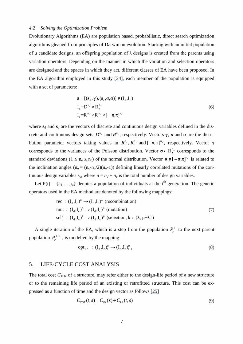
4.2 Solving the Optimization Problem

Evolutionary Algorithms (EA) are population based, probabilistic, direct search optimization

algorithms gleaned from principles of Darwinian evolution. Starting with an initial population

of μ candidate designs, an offspring population of λ designs is created from the parents using

variation operators. Depending on the manner in which the variation and selection operators

are designed and the spaces in which they act, different classes of EA have been proposed. In

the EA algorithm employed in this study [24], each member of the population is equipped

with a set of parameters:

γd

c σ

d c d c

nn

d

n n n

c

[( , , ( , , )] (Ι ,Ι )

Ι =D R

Ι =R R [ π,π] a

a s γ s σ α

(6)

where sd and sc are the vectors of discrete and continuous design variables defined in the dis-

crete and continuous design sets n n and d cD R , respectively. Vectors γ, σ and α are the distri-

bution parameter vectors taking values in n n n

, and [ , ] ,aR R respectively. Vector γ

corresponds to the variances of the Poisson distribution. Vector σnRσ corresponds to the

standard deviations (1 nσ nc) of the normal distribution. Vector n

[ π,π] aα is related to

the inclination angles (nα = (nc-nσ/2)(nσ-1)) defining linearly correlated mutations of the con-

tinuous design variables sc, where n = nd + nc is the total number of design variables.

Let P(t) = {a1,…,aμ} denotes a population of individuals at the tth

generation. The genetic

operators used in the EA method are denoted by the following mappings:

μ λ

d c d c

λ λ

d c d c

k k μ

μ d c d c

rec : (Ι ,Ι ) (Ι ,Ι ) (recombination)

mut : (Ι ,Ι ) (Ι ,Ι ) (mutation)

sel : (Ι ,Ι ) (Ι ,Ι ) (selection, k {λ, μ+λ})

(7)

A single iteration of the EA, which is a step from the population P tp to the next parent

population P t+1p , is modelled by the mapping

μ μ

EA d c t d c t+1opt : (Ι ,Ι ) (Ι ,Ι ) (8)

5. LIFE-CYCLE COST ANALYSIS

The total cost CTOT of a structure, may refer either to the design-life period of a new structure

or to the remaining life period of an existing or retrofitted structure. This cost can be ex-

pressed as a function of time and the design vector as follows [25]

( , ) ( ) ( , )TOT IN LSC t C C ts s s (9)

8

where CIN is the initial cost of a new or retrofitted structure, CLS is the present value of the

limit state cost; s is the design vector corresponding to the design loads, resistance and mate-

rial properties, while t is the time period. The term “initial cost” of a new structure refers to

the cost just after construction. The initial cost is related to the material and the labour cost for

the construction of the building which includes concrete, steel reinforcement, labour cost for

placement as well as the non-structural component cost. The term “limit state cost” refers to

the potential damage cost from earthquakes that may occur during the life of the structure. It

accounts for the cost of the repairs after an earthquake, the cost of loss of contents, the cost of

injury recovery or human fatality and other direct or indirect economic losses related to loss

of contents, rental and income. The quantification of the losses in economical terms depends

on several socio-economic parameters. It should be mentioned that in the calculation formula

of CLS a regularization factor is used that transforms the costs in present values. The most dif-

ficult cost to quantify is the cost corresponding to the loss of a human life. In this work the

fatality cost is based on the legal damages that the courts adjudge in the case of loss of life.

Damage may be quantified by using several damage indices (DIs) whose values can be re-

lated to particular structural damage states. The idea of describing the state of damage of the

structure by a specific number, on a defined scale in the form of a damage index, is attractive

because of its simplicity. So far a significant number of researchers has studied various dam-

age indices for reinforced concrete or steel structures, a detailed survey can be found in the

work by Ghobarah et al. [26]. Damage, in the context of life cycle cost analysis (LCCA),

means not only structural damage but also non-structural damage. The latter including the

case of architectural damage, mechanical, electrical and plumbing damage and also the dam-

age of furniture, equipment and other contents. The maximum interstory drift (θ) has been

considered as the response parameter which best characterises the structural damage, which

has been associated with all types of losses. It is generally accepted that interstorey drift can

be used as one limit state criterion to determine the expected damage. The relation between

the drift ratio limits with the limit state, employed in this study (Table 1), is based on the work

of Ghobarah [27] for ductile RC moment resisting frames. On the other hand, the intensity

measure associated with the loss of contents like furniture and equipment is the maximum re-

sponse floor acceleration. The relation of the limit state with the values of the floor accelera-

tion used in this work (Table 1) are based on the work of Elenas and Meskouris [28].

The limit state cost (CLS), for the i-th limit state, can thus be expressed as follows

, ,i i i i i i i

LS dam con ren inc inj fatC C C C C C C (10a)

, ,i acc i acc

LS conC C (10b)

9

where i

damC is the damage repair cost, ,i

conC is the loss of contents cost due to structural dam-

age that is quantified by the maximum interstorey drift, i

renC is the loss of rental cost, i

incC is

the income loss cost, i

injC is the cost of injuries and i

fatC is the cost of human fatality. These

cost components are related to the damage of the structural system. ,i acc

conC is the loss of con-

tents cost due to floor acceleration [28]. Details about the calculation formula for each limit

state cost along with the values of the basic cost for each category can be found in Table 2

[29,30]. The values of the mean damage index, loss of function, down time, expected minor

injury rate, expected serious injury rate and expected death rate used in this study are based on

[31-34]. Table 3 provides the ATC-13 [32] and FEMA-227 [33] limit state dependent damage

consequence severities.

Based on a Poisson process model of earthquake occurrences and an assumption that dam-

aged buildings are immediately retrofitted to their original intact conditions after each major

damage-inducing seismic attack, Wen and Kang [25] proposed the following formula for the

limit state cost function considering N limit states

acc

LS LS LSC C C

(11a)

,

1

( , ) 1N

t i

LS LS i

i

C t e C Ps (11b)

,

1

( , ) 1N

acc t i acc acc

LS LS i

i

C t e C Ps

(11c)

where

1( ) ( )DI

i i iP P DI DI P DI DI (12)

and

( ) ( 1 / ) ln[1 ( )]i i iP DI DI t P DI DI (13)

Pi is the probability of the ith

limit state being violated given the earthquake occurrence and

i

LSC is the corresponding limit state cost; ( )iP DI DI is the exceedance probability given

occurrence; DIi, DIi+1 are the damage indices (maximum interstorey drift or maximum floor

acceleration) defining the lower and upper bounds of the ith

limit state; ( )i iP DI DI is the an-

nual exceedance probability of the maximum damage index DIi; ν is the annual occurrence

rate of significant earthquakes modelled by a Poisson process and t is the service life of a new

structure or the remaining life of a retrofitted structure. Thus, for the calculation of the limit

state cost of Eq. (11b) the maximum interstorey drift DI is considered, while for the case of

Eq. (11b) the maximum floor acceleration is used. The first component of Eqs. (11b) or (11c),

with the exponential term, is used in order to express CLS in present value, where λ is the an-

nual monetary discount rate. In this work the annual monetary discount rate λ is taken to be

10

constant, since considering a continuous discount rate is accurate enough for all practical pur-

poses according to Rackwitz [35,36]. Various approaches yield values of the discount rate λ in

the range of 3 to 6% [31], in this study it was taken equal to 5%.

Each limit state is defined by drift ratio limits or floor acceleration, as listed in Table 1.

When one of the DIs is exceeded the corresponding limit state is assumed to be reached. The

annual exceedance probability ( )i iP DI DI is obtained from a relationship of the form

( ) ( ) k

i i iP DI DI DI (14)

The above expression is obtained by best fit of known i iP DI pairs for each of the two DIs.

These pairs correspond to the 2, 10 and 50 percent in 50 years earthquakes that have known

probabilities of exceedance iP . In this work the maximum value of DIi (interstorey drift or

floor acceleration) corresponding to the three hazard levels considered, are obtained through a

number of non-linear dynamic analyses. The selection of the proper external loading for de-

sign and/or assessment purposes is not an easy task due to the uncertainties involved in the

seismic loading. For this reason a rigorous treatment of the seismic loading is to assume that

the structure is subjected to a set of records that are more likely to occur in the region where

the structure is located. In our case as a series of twenty artificial accelerograms per hazard

level is implemented.

According to Poisson’s law the annual probability of exceedance of an earthquake with a

probability of exceedance p in t years is given by the formula

( 1/ ) ln(1 )P t p (15)

This means that the 2/50 earthquake has a probability of exceedance equal to 2%P = - ln(1-

0.02)/50 = 4.04×10-4

(4.04×10-2

%).

6. NON-LINEAR DYNAMIC ANALYSIS PROCEDURE

In order to define the i iP DI pairs for the two DIs, three performance levels are considered

and twenty ground motion records are selected for each hazard level. Sixty non-linear dy-

namic analyses have to be performed for each candidate design in order to assess its perform-

ance in the framework of LCCA. Although, strong motion recording programs have been

carried out in US over the last 60 years, and more recently in many parts of the world; for

many applications, it is necessary to estimate future seismic records in multiple hazard levels

at a particular site, which is often outside the existing recorded data. For the present investiga-

tion a number of records for each 50/50, 10/50 and 2/50 hazard level were required for the

region of Eastern Mediterranean. These records were not possible to be found in any database,

thus artificial ground motions, compatible with the corresponding design spectrum, were gen-

erated for each hazard level. Apart from enriching the catalogues of earthquake records of a

11

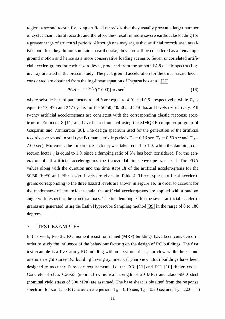
region, a second reason for using artificial records is that they usually present a larger number

of cycles than natural records, and therefore they result in more severe earthquake loading for

a greater range of structural periods. Although one may argue that artificial records are unreal-

istic and thus they do not simulate an earthquake, they can still be considered as an envelope

ground motion and hence as a more conservative loading scenario. Seven uncorrelated artifi-

cial accelerograms for each hazard level, produced from the smooth EC8 elastic spectra (Fig-

ure 1a), are used in the present study. The peak ground acceleration for the three hazard levels

considered are obtained from the log-linear equation of Papazachos et al. [37]

+ ln( ) 2= e (/1000) [m / sec ]ma b TPGA (16)

where seismic hazard parameters a and b are equal to 4.01 and 0.61 respectively, while Tm is

equal to 72, 475 and 2475 years for the 50/50, 10/50 and 2/50 hazard levels respectively. All

twenty artificial accelerograms are consistent with the corresponding elastic response spec-

trum of Eurocode 8 [11] and have been simulated using the SIMQKE computer program of

Gasparini and Vanmarcke [38]. The design spectrum used for the generation of the artificial

records correspond to soil type B (characteristic periods ΤB = 0.15 sec, ΤC = 0.50 sec and ΤD =

2.00 sec). Moreover, the importance factor γI was taken equal to 1.0, while the damping cor-

rection factor η is equal to 1.0, since a damping ratio of 5% has been considered. For the gen-

eration of all artificial accelerograms the trapezoidal time envelope was used. The PGA

values along with the duration and the time steps Δt of the artificial accelerograms for the

50/50, 10/50 and 2/50 hazard levels are given in Table 4. Three typical artificial accelero-

grams corresponding to the three hazard levels are shown in Figure 1b. In order to account for

the randomness of the incident angle, the artificial accelerograms are applied with a random

angle with respect to the structural axes. The incident angles for the seven artificial accelero-

grams are generated using the Latin Hypercube Sampling method [39] in the range of 0 to 180

degrees.

7. TEST EXAMPLES

In this work, two 3D RC moment resisting framed (MRF) buildings have been considered in

order to study the influence of the behaviour factor q on the design of RC buildings. The first

test example is a five storey RC building with non-symmetrical plan view while the second

one is an eight storey RC building having symmetrical plan view. Both buildings have been

designed to meet the Eurocode requirements, i.e. the EC8 [11] and EC2 [10] design codes.

Concrete of class C20/25 (nominal cylindrical strength of 20 MPa) and class S500 steel

(nominal yield stress of 500 MPa) are assumed. The base shear is obtained from the response

spectrum for soil type B (characteristic periods ΤB = 0.15 sec, ΤC = 0.50 sec and ΤD = 2.00 sec)

12

while the PGA considered is equal to 0.31 g. Moreover, the importance factor γI was taken

equal to 1.0, while the damping correction factor is equal to 1.0, since a damping ratio of 5%

has been considered.

The slab thickness is equal to 15 cm, for both test examples, while it is considered to con-

tribute to the moment of inertia of the beams with an effective flange width. In addition to the

self weight of beams and slabs, a distributed permanent load of 2 kN/m2 due to floor finish-

ing-partitions and an imposed load with nominal value of 1.5 kN/m2, are considered. The

nominal permanent and imposed loads are multiplied by load factors of 1.35 and 1.5, respec-

tively. Following EC8, in the seismic design combination, dead loads are considered with

their nominal values, while live loads with the 30% of their nominal value.

In both test examples the parametric study is performed in two stages: (i) design based on

structural optimization and (ii) life-cycle cost analysis. In the first stage the optimum design is

computed employing the EA(μ+λ) optimization scheme [24] with ten parent and offspring

(μ=λ=10) design vectors for both test examples. Four optimization problems are defined, fol-

lowing the design recommendations of EC8 and EC2, according to the value of the behaviour

factor considered. The optimum designs obtained are labelled as Dq=a defining the value of

the behaviour factor used. In all formulations the initial construction cost is the objective

function to be minimized. The columns and beams are of rectangular cross-sectional shape,

and are separated into groups. The two dimensions of the columns/beams along with the lon-

gitudinal, transverse reinforcement and its spacing are the five design variables that are as-

signed to each group of the columns/beams. In the second stage, life-cycle cost analysis is

performed on the optimum designs by means of non-linear dynamic analysis where the beam-

column members are modelled with the inelastic force-based fibre element [40].

7.1. Five storey non-symmetrical test example

The plan and front views of the five storey non-symmetrical test example are shown in Figure

2. The structural elements (beams and columns) are separated into 10 groups, 8 for the col-

umns and 2 for the beams, resulting into 50 design variables. The optimum designs achieved

for different values of the q factor are presented in Table 5. It can be seen that the initial con-

struction cost of design Dq=1 is increased by the marginal quantity of 7% compared to Dq=2,

while it is 10% and 12% more expensive compared to Dq=3 and Dq=4, respectively. It can

therefore be said that the initial cost of RC structures, designed on the basis of their elastic

response for the design earthquake, is not excessive taking into consideration the additional

costs of a building structure which are practically the same for all designs q=1 to 4. When the

four designs are compared with respect to the cost of the RC skeletal members, design Dq=1 is

13

increased by 40% compared to Dq=2 and by 67% and 92% compared to Dq=3 and Dq=4, respec-

tively.

Table 3 provides the ATC-13 [32] and FEMA-227 [33] limit state dependent parameters

required for the calculation of the following costs: damage repair, loss of contents, loss of

rental, income loss, cost of injuries and that of human fatality. The computed components of

the limit states, for the five storey RC building, are listed in Table 6. From Table 6 it can be

seen that damage and income loss costs are the dominating cost components for the limit

states I through VI representing, by average, the 83% of i

LSC , while the cost of human fatality

is the dominant cost (73%) at the highest limit state VII. Below it is explained the calculation

procedure of the limit state cost taking as an example the design corresponding to Dq=3. In the

first step three ( )i iP and three ,( )i floor iP u pairs are defined corresponding to the three

hazard levels

50% 50% ,50%

1

10% 10% ,10%

2

2% 2% ,2%

1.39% 0.14 % 0.36

2.10 10 % 0.42 % 0.96

4.04 10 % 1.24 % 2.18

floor

floor

floor

P u g

P u g

P u g

(17)

The abscissa values for both ( )i iP and ,( )i floor iP u pairs, corresponding to the median

values of the maximum interstorey drifts and maximum floor accelerations for the three haz-

ard levels in question, are obtained through 20 non-linear time history analyses performed for

each hazard level 50/50, 10/50 and 2/50. The median values of the four designs are shown in

Figures 3(a) and 3(b). The ordinate values, corresponding to the annual probabilities of ex-

ceedance, are calculated using Eq. (15). Subsequently, exponential functions for the two DIs,

as the one described in Eq. (14), is fitted to the pairs of Eq. (17). Once the two functions of

the best fitted curve are defined the annual probabilities of exceedance iP for each of the

seven limit states of Table 1 are calculated. Substituting iP into Eq. (13) the exceedance prob-

abilities of the limit state given occurrence are computed and the probabilities Pi are then

evaluated from Eq. (12). This procedure is performed for each one of the DIs, i.e. interstorey

drifts and floor accelerations. The limit state cost of Eq. (11a) is calculated adding the two

components of Eqs. (11b) and (11c), while these two components are defined combining the

numerical values of the cost components of Table 6 and the corresponding probabilities Pi.

Figure 4 depicts the optimum designs obtained with reference to the behaviour factor,

along with the initial construction, limit state and total life-cycle costs. It can be observed

from this figure that although design Dq=1 is worst, compared to the other three designs with

reference to CIN, with respect to CTOT the design Dq=4 is the most expensive. Comparing de-

sign Dq=3, obtained for the behaviour factor suggested by the Eurocodes for RC buildings,

14

with reference to CTOT, it can be seen that it is 50% and 20% more expensive compared to

Dq=1 and Dq=2, respectively; while it is 10% less expensive compared to Dq=4.

The contribution of the initial and limit state cost components to the total life-cycle cost are

shown in Figure 5. CIN represents the 75% of the total life-cycle cost for design Dq=1 while for

designs Dq=2, Dq=3 and Dq=4 represents the 59%, 50% and 45%, respectively. Although the

initial cost is the dominant contributor for all optimum design; for design Dq=1 the second

dominant contributor is the cost of contents due to floor acceleration while for designs Dq=2,

Dq=3 and Dq=4 damage and income costs are almost equivalent representing the second domi-

nant contributors. It is worth mentioning, that the contribution of the cost of contents due to

floor acceleration on the limit-state cost is only 20% for design Dq=4 while it is almost 85%

for design Dq=1. This is due to the fact that the latter design is much stiffer and thus increased

floor accelerations inflict significant damages on the contents. It has also to be noticed that

although the four designs differ significantly, injury and fatality costs represent only a small

quantity of the total cost: 0.015% for design Dq=1 , while for designs Dq=2, Dq=3 and Dq=4

represents the 0.25%, 1.0% and 2.3% of the total cost, respectively.

7.2. Eight storey symmetrical test example

The plan and front views of the eight storey symmetrical test example are shown in Figure 6.

The structural elements (beams and columns) are separated into 14 groups, 12 groups for the

columns and 2 for the beams, resulting into 70 design variables. The optimum designs

achieved for different values of the q factor are presented in Table 7. It can be seen that, with

respect to total initial cost design Dq=1 is increased by the marginal quantity of 3% compared

to Dq=2 and by 10% and 15% compared to Dq=3 and Dq=4, respectively. In the case when the

four designs are compared with reference to the cost of the RC skeletal members alone, de-

sign Dq=1 is increased by 12% compared to Dq=2 and by 65% and 95% compared to Dq=3 and

Dq=4, respectively. Confirming the results of the first test example, it can be also seen that the

initial construction cost of RC structures designed based on elastic response for the design

earthquake is by no means prohibitive

The median values of the four cases employed for defining the abscissa values of both

( )i iP and ,( )i floor iP u pairs, are shown in Figures 7(a) and 7(b), while they have been ob-

tained through 20 non-linear time history analyses performed for each of the three hazard le-

vels (50/50, 10/50 and 2/50). Figure 8 depicts the optimum designs obtained with reference to

the four behaviour factors, along with the initial construction, limit state and total life-cycle

costs, calculated for the Ghobarah drift limits [27]. In accordance to the previous test example,

a general observation can be obtained from this figure that design Dq=4 is worst compared to

the other three designs with respect to CTOT. Comparing design Dq=3, obtained for the behav-

15

iour factor suggested by the Eurocodes for RC buildings, it can be seen that it is 30% and

17% more expensive compared to Dq=1 and Dq=2, respectively; while it is 6%, less expensive

with reference to CTOT, compared to Dq=4.

The contribution of the initial and limit state cost components to the total life-cycle cost are

shown in Figure 9. CIN represents the 72% of the total life-cycle cost for design Dq=1 while for

designs Dq=2, Dq=3 and Dq=4 represents the 65%, 54% and 50%, respectively. Although the

initial cost is the dominant contributor for all optimum design; for designs Dq=1 and Dq=2 the

second dominant contributor is the cost of contents due to floor acceleration while for designs

Dq=3 and Dq=4 damage and income costs are almost equivalent representing the second domi-

nant contributors. It is worth mentioning, as in the previous example, that the contribution of

the cost of contents due to floor acceleration on the limit-state cost is only 29%, as in the pre-

vious example, for design Dq=4 while it is almost 76% for design Dq=1. Furthermore, although

the four designs differ significantly injury and fatality costs represent only a small quantity of

the total cost: 0.041% for design Dq=1, while for designs Dq=2, Dq=3 and Dq=4 represents the

0.14%, 0.46% and 0.68% of the total cost, respectively.

8. CONCLUDING REMARKS

An investigation was performed on the effect of the behaviour factor q in the final design of

reinforced concrete buildings under earthquake loading in terms of safety and economy. The

numerical tests were performed on two multi-storey reinforced concrete buildings having

symmetrical and non symmetrical plan views which were optimally designed according the

European codes EC2 and EC8. The values of the behaviour factor varied from q=1, represent-

ing the elastic response, to q=4. Although the two test examples are different this study re-

sulted in quite similar findings for the two cases considered.

The main findings of this study can be summarized in the following:

1. The initial cost of reinforced concrete structures designed based on elastic response

Dq=1 is not excessive since it varies, for the two representative test cases considered,

from 3% to 15% compared to the initial cost of the designs Dq=2 to Dq=4, respectively.

In fact, the designs Dq=1 are only by 10% more expensive compared to the cost of the

designs obtained for the value of the behaviour factor suggested by the Eurocode

(q=3). In the case, though, that the four designs are compared with reference to the

cost of the RC skeletal members alone, design Dq=1 is 95% more expensive compared

to Dq (q=2,3,4).

2. Comparing, the contributing parts (Figures 5 and 9) of the total life-cycle cost, it can

be said that the initial cost, in both test examples, is the first dominant contributor for

16

all designs obtained. The cost of contents due to floor acceleration is the second domi-

nant contributor for stiffer design (Dq=1 and Dq=2), while for designs Dq=3 and Dq=4

damage and income costs are almost equivalent representing the second dominant con-

tributors. It is also worth mentioning that, although the four designs differ significantly,

injury and fatality costs represent only a small percentage of the total cost.

3. The contribution of the cost of contents due to floor acceleration on the limit-state cost

was in the range 20% to 29% for design Dq=4 while it was found in the range 76% to

85% for design Dq=1. This is due to the fact that the latter design is much stiffer com-

pared to the other ones and thus increased floor accelerations inflict significant dam-

ages on the contents.

4. The main conclusion that can be drawn from this study is that the behavior factor sug-

gested by the Eurocode does not lead to the most safe and economic design.

ACKNOWLEDGMENTS

The first author acknowledges the financial support of the John Argyris Foundation.

REFERENCES

[1] Fajfar, P. Towards nonlinear methods for the future seismic codes, In Seismic design practice

into the next century, Booth (Ed.), Balkema, 1998.

[2] Mazzolani, FM, Piluso, V. The theory and design of seismic resistant steel frames, E & FN

Spon, 1996.

[3] ATC-19, Structural response modification factors, Applied Technology Council: Redwood City,

CA, 1995.

[4] Frangopol, D.M. Computer-automated design of structural systems under reliability-based per-

formance constraints. Engineering Computations 1986; 3(2): 109–115.

[5] Moharrami, H., Grierson, D.E. Computer-automated design of reinforced concrete frameworks.

Journal of Structural Engineering 1993; 119(7): 2036–2058.

[6] Sarma, K.C., Adeli, H. Cost optimization of concrete structures. Journal of Structural Engineer-

ing 1998; 124(5): 570–578.

[7] Li, G., Cheng, G. Optimal decision for the target value of performance-based structural system

reliability. Structural & Multidisciplinary Optimization 2001; 22(4): 261–267.

[8] Chan, C.-M., Zou, X.-K. Elastic and inelastic drift performance optimization for reinforced con-

crete buildings under earthquake loads. Earthquake Engineering & Structural Dynamics 2004;

33(8): 929–950.

[9] Lagaros, N.D., Papadrakakis, M. Seismic design of RC structures: a critical assessment in the

framework of multi-objective optimization. Earthquake Engineering & Structural Dynamics

2007; 36(12): 1623–1639.

[10] PrEN 1992-1-1:2002. Eurocode 2: Design of Concrete Structures- Part 1: General Rules and

Rules for Buildings. Commission of the European Communities, European Committee for Stan-

dardization, December 2002.

[11] EN 1998-1:2003. Eurocode 8: Design of Structures for Earthquake Resistance. Part 1: General

rules, seismic actions and rules for buildings. Commission of the European Communities, Euro-

pean Committee for Standardization, October 2003.

[12] ATC-34. A critical review of current approaches to earthquake resistance design. Applied Tech-

nology Council: Redwood City, CA, 1995.

17

[13] Palazzo B, Petti L. Reduction factors for base isolated structures. Computers and Structures

1996; 60(6): 945–956

[14] Borzi, B., Elnashai, A.S. Refined force reduction factors for seismic design. Engineering Struc-

tures 2000; 22(10): 1244–1260.

[15] Whittaker A, Hart G, Rojahn C. Seismic response modification factors. Journal of Structural

Engineering 1999; 125(4): 438–444

[16] Kappos AJ. Evaluation of behaviour factors on the basis of ductility and overstrength studies.

Engineering Structures 1999; 21(9): 823-835.

[17] Lu Y, Hao H, Carydis P. G, Mouzakis, H. Seismic performance of RC frames designed for three

different ductility levels. Engineering Structures 2001; 23(5): 537–547

[18] Miranda, E., Bertero, V.V. Evaluation of strength reduction factors for earthquake resistant de-

sign. Earthquake Spectra 1994; 10(2): 357–379.

[19] Lam, N., Wilsont, J., Hutchinson, G. The ductility reduction factor in the seismic design of

buildings. Earthquake Engineering & Structural Dynamics 1998; 27: 749–769.

[20] Cuesta, I., Aschheim, M.A., Fajfar, P. Simplified R-factor relationships for strong ground mo-

tions. Earthquake Spectra 2003; 19(1): 25–45.

[21] Lee, K., Foutch, D.A. Seismic evaluation of steel moment frame buildings designed using dif-

ferent R-values. Journal of Structural Engineering 2006; 132(9): 1461–1472.

[22] Karavasilis, T.L., Bazeos, N., Beskos, D.E. Behaviour factor for performance-based seismic

design of plane steel moment resisting frames. Journal of Earthquake Engineering 2007; 11(4):

531–559.

[23] Karakostas, C.Z., Athanassiadou, C.J., Kappos, A.J., Lekidis, V.A. Site-dependent design spec-

tra and strength modification factors, based on records from Greece. Soil Dynamics and Earth-

quake Engineering 2007; 27 (11): 1012–1027.

[24] Lagaros, N.D., Garavelas, A.Th., Papadrakakis, M. Innovative seismic design optimization with

reliability constraints, Computer Methods in Applied Mechanics and Engineering 2008; 198(1):

28-41.

[25] Wen YK, Kang YJ. Minimum building life-cycle cost design criteria. I: Methodology. Journal

of Structural Engineering 2001; 127(3): 330–337.

[26] Ghobarah A, Abou-Elfath H, Biddah A. Response-based damage assessment of structures.

Earthquake Engineering & Structural Dynamics 1999, 28(1): 79-104.

[27] Ghobarah A. On drift limits associated with different damage levels. International Workshop on

Performance-Based Seismic Design, June 28 - July 1, 2004.

[28] Elenas A, Meskouris K. Correlation study between seismic acceleration parameters and damage

indices of structures, Engineering Structures 2001, 23: 698–704.

[29] Wen YK, Kang YJ. Minimum building life-cycle cost design criteria. II: Applications. Journal

of Structural Engineering 2001; 127(3):338-346.

[30] Lagaros, N.D. Life-cycle cost analysis of construction practices, Bulletin of Earthquake Engi-

neering 2007; 5, 425-442.

[31] Ellingwood BR, Wen Y-K. Risk-benefit-based design decisions for low-probability/high conse-

quence earthquake events in mid-America. Progress in Structural Engineering and Materials

2005; 7(2): 56–70.

[32] ATC-13. Earthquake Damage Evaluation Data for California. Applied Technology Council:

Redwood City, CA, 1985.

[33] FEMA 227. A Benefit–Cost Model for the Seismic Rehabilitation of Buildings. Federal Emer-

gency Management Agency, Building Seismic Safety Council: Washington, DC, 1992.

[34] Kang Y-J, Wen YK (2000). Minimum life-cycle cost structural design against natural hazards,

Structural Research Series No. 629. Department of Civil and Environmental Engineering, Uni-

versity of Illinois at Urbana-Champaign, Urbana, IL.

[35] Rackwitz R. The effect of discounting, different mortality reduction schemes and predictive co-

hort life tables on risk acceptability criteria, Reliability Engineering and System Safety 2006;

91(4): 469–484.

[36] Rackwitz R, Lentz A, Faber M. Socio-economically sustainable civil engineering infrastructures

by optimization. Structural Safety 2005; 27(3): 187-229.

18

[37] Papazachos BC, Papaioannou ChA, Theodulidis NP. Regionalization of seismic hazard in

Greece based on seismic sources. Natural Hazards 1993; 8(1): 1-18.

[38] Gasparini DA, Vanmarcke EH. Simulated earthquake motions compatible with prescribed re-

sponse spectra. MIT civil engineering research report R76-4. Massachusetts Institute of Tech-

nology, Cambridge, MA, 1976.

[39] Olsson A, Sandberg G, Dahlblom O. On latin hypercube sampling for structural reliability

analysis. Structural Safety 2003; 25(1), 47-68.

[40] Papaioannou I, Fragiadakis M, Papadrakakis M. Inelastic Analysis of framed structures using

the fiber approach, Proceedings of the 5th International Congress on Computational Mechanics

(GRACM 05), Limassol, Cyprus, June 29 - July 1, 2005.

19

TABLES

Table 1: Limit state drift ratio limits for bare Moment Resisting Frames and contents DI

Limit

State

Interstorey Drift (%)

[27]

Contents DI (g)

[28]

(I) - None θ ≤0.1 üfloor ≤0.05

(II) - Slight 0.1< θ ≤0.2 0.05< üfloor ≤0.10

(III) - Light 0.2< θ ≤0.4 0.10< üfloor ≤0.20

(IV) - Moderate 0.4< θ ≤1.0 0.20< üfloor ≤0.80

(V) - Heavy 1.0< θ ≤1.8 0.80< üfloor ≤0.98

(VI) - Major 1.8< θ ≤3.0 0.98< üfloor ≤1.25

(VII) - Collapsed θ >3.0 üfloor >1.25

Table 2: Limit state costs - calculation formula [31-34]

Cost Category Calculation Formula Basic Cost

Damage/repair (Cdam) Replacement cost × floor area × mean damage index 1500 €/m2

Loss of contents (Ccon) Unit contents cost × floor area × mean damage index 500 €/m2

Rental (Cren) Rental rate × gross leasable area × loss of function 10 €/month/m2

Income (Cinc) Rental rate × gross leasable area × down time 2000 €/year/m2

Minor Injury (Cinj,m) Minor injury cost per person × floor area × occupancy

rate × expected minor injury rate 2000 €/person

Serious Injury (Cinj,s) Serious injury cost per person × floor area × occupancy

rate × expected serious injury rate 2×10

4 €/person

Human fatality (Cfat) Human fatality cost per person × floor area × occu-

pancy rate × expected death rate 2.8×10

6 €/person

* Occupancy rate 2 persons/100 m2

Table 3: Limit state parameters for cost evaluation

Limit

State

FEMA-227 [33] ATC-13 [32]

mean

damage

index (%)

expected

minor in-

jury rate

expected

serious

injury rate

expected

death rate

loss of

function

(%)

down time

(%)

(I) - None 0 0 0 0 0 0

(II) - Slight 0.5 3.0E-05 4.0E-06 1.0E-06 0.9 0.9

(III) - Light 5 3.0E-04 4.0E-05 1.0E-05 3.33 3.33

(IV) - Moderate 20 3.0E-03 4.0E-04 1.0E-04 12.4 12.4

(V) - Heavy 45 3.0E-02 4.0E-03 1.0E-03 34.8 34.8

(VI) - Major 80 3.0E-01 4.0E-02 1.0E-02 65.4 65.4

(VII) - Collapsed 100 4.0E-01 4.0E-01 2.0E-01 100 100

20

Table 4: Artificial ground motion characteristics.

Hazard Level PGA (g) Duration (sec) No of Steps Δt (sec)

50/50 0.11 20.5 1024 2.00E-02

10/50 0.31 30.5 2048 1.49E-02

2/50 0.78 35.5 4096 8.67E-03

Table 5: Five storey test example - Optimum designs obtained for different values of behaviour factor q

Optimum Designs

q=1 q=2 q=3 q=4

Co

lum

ns

h1×b1 0.80×0.80, LR: 34Ø32,

TR: (4)Ø10/10cm

0.60×0.60, LR:8Ø24+

12Ø28, TR: (4)Ø10/20cm

0.55×0.55, LR:8Ø20+

12Ø24, TR: (2)Ø10/20cm

0.55×0.55, LR:8Ø24+

4Ø28, TR: (2)Ø10/20cm

h2×b2 0.85×0.85, LR: 34Ø32,

TR: (4)Ø10/10cm

0.60×0.60, LR:8Ø24+

12Ø28, TR: (4)Ø10/20cm

0.55×0.55, LR:8Ø22+

12Ø26, TR: (2)Ø10/20cm

0.55×0.55, LR:8Ø24+

4Ø28, TR: (2)Ø10/20cm

h3×b3 0.80×0.80, LR: 28Ø32,

TR: (4)Ø10/10cm

0.60×0.60, LR:8Ø24+

12Ø28, TR: (4)Ø10/20cm

0.50×0.50, LR:4Ø22+

12Ø26, TR: (2)Ø10/20cm

0.50×0.50, LR:4Ø26+

4Ø32, TR: (2)Ø10/20cm

h4×b4 0.70×0.70, LR:8Ø22+

12Ø26, TR: (4)Ø10/10cm

0.55×0.55, LR:8Ø24+

12Ø28, TR: (4)Ø10/20cm

0.55×0.55, LR:8Ø18+

4Ø22, TR: (2)Ø10/20cm

0.55×0.55, LR:8Ø18+

4Ø22, TR: (2)Ø10/20cm

h5×b5 0.70×0.70,LR: 26Ø32, TR:

(4)Ø10/10cm

0.55×0.55, LR:4Ø28+

8Ø24, TR: (4)Ø10/20cm

0.55×0.55, LR:8Ø24+

4Ø28, TR: (2)Ø10/20cm

0.55×0.55, LR:8Ø20+

4Ø24, TR: (2)Ø10/20cm

h6×b6 0.70×0.70, LR: 24Ø32,

TR: (4)Ø10/10cm

0.50×0.55, LR:12Ø28+

8Ø24, TR: (4)Ø10/20cm

0.45×0.45, LR:4Ø24+

4Ø28, TR: (2)Ø10/20cm

0.45×0.45, LR:4Ø26+

4Ø32, TR: (2)Ø10/20cm

h7×b7 0.65×0.65, LR:15Ø18+

16Ø20, TR: (4)Ø10/10cm

0.35×0.60, LR:8Ø18+

8Ø20, TR: (2)Ø10/20cm

0.35×0.55, LR:7Ø16+

5Ø20, TR: (2)Ø10/20cm

0.50×0.30, LR:5Ø18+

6Ø16, TR: (2)Ø10/20cm

h8×b8 0.60×0.65, LR:24Ø20+

20Ø18, TR:(4)Ø10/10cm

0.40×0.60, LR: 18Ø18,

TR: (2)Ø10/20cm

0.35×0.55, LR:8Ø18+

5Ø20, TR: (2)Ø10/20cm

0.55×0.30, LR:8Ø18,

TR: (2)Ø10/20cm

Beams h9×b9

0.45×0.55,LR: 15Ø20, TR:

(2)Ø10/10cm

0.30×0.50, LR: 9Ø18, TR:

(2)Ø10/20cm

0.30×0.55, LR:3Ø20+

4Ø14, TR: (2)Ø10/20cm

0.25×0.45, LR:4Ø16+

4Ø14, TR: (2)Ø10/20cm

h10×b10 0.50×0.55, LR: 24Ø18,

TR: (2)Ø8/15cm

0.30×0.55, LR: 10Ø18,

TR: (2)Ø8/15cm

0.30×0.55, LR:6Ø20, TR:

(2)Ø8/15cm

0.25×0.45, LR:4Ø16, TR:

(2)Ø8/15cm

CIN, RC Frame (1000 €) 1.85E+02 1.32E+02 1.11E+02 9.62E+01

CIN (1000 €) 8.10E+02 7.57E+02 7.36E+02 7.21E+02

Table 6: Five storey test example - Limit state cost components (1000 €)

Limit

State

i

damC

i

conC

i

renC

i

incC

i

injC i

fatC i

LSC (I)

i

LSC (II)

Minor Serious

I 0.00 0.00 0.00 0.00 0.00 0.00 0.00 0.00 0.00

II 9.38 3.13 1.35 22.50 0.00 0.00 0.07 36.35 36.42

III 93.75 31.25 5.00 83.25 0.02 0.02 0.70 213.25 213.98

IV 375.00 125.00 18.60 310.00 0.15 0.20 7.00 828.60 835.95

V 843.75 281.25 52.20 870.00 1.50 2.00 70.00 2047.20 2120.70

VI 1500.00 500.00 98.10 1635.00 15.00 20.00 700.00 3733.10 4468.10

VII 1875.00 625.00 150.00 2500.00 20.00 200.00 14000.00 5150.00 19370.00

21

Table 7: Eight storey test example - Optimum designs obtained for different values of behaviour fac-

tor q

Optimum Designs

q=1 q=2 q=3 q=4

Co

lum

ns

h1×b1 1.35×1.35, LR: 88Ø30,

TR: (5)Ø10/10cm

0.80×0.75, LR: 26Ø32,

TR: (4)Ø10/15cm

0.80×0.60, LR: 24Ø28,

TR: (4)Ø10/20cm

0.80×0.60, LR:10Ø24+

12Ø28, TR: (2)Ø10/20cm

h2×b2 0.90×0.85, LR: 34Ø30,

TR: (4)Ø10/10cm

0.80×0.80, LR: 30Ø32,

TR: (4)Ø10/10cm

0.65×0.60, LR: 26Ø28,

TR: (4)Ø10/20cm

0.75×0.35, LR:8Ø22+

12Ø26, TR: (2)Ø10/20cm

h3×b3 1.05×1.10, LR: 50Ø30,

TR: (4)Ø10/10cm

0.80×0.80, LR: 30Ø32,

TR: (4)Ø10/10cm

0.75×0.65, LR: 28Ø28,

TR: (4)Ø10/20cm

0.75×0.70, LR:10Ø22+

12Ø26, TR: (2)Ø10/20cm

h4×b4 1.10×1.05, LR: 60Ø30,

TR: (4)Ø10/10cm

0.80×0.85, LR: 32Ø32,

TR: (4)Ø10/10cm

0.75×0.65, LR: 30Ø28,

TR: (4)Ø10/15cm

0.70×0.65, LR:8Ø26+

12Ø32, TR: (2)Ø10/20cm

h5×b5 0.85×0.85, LR: 36Ø30,

TR: (4)Ø10/10cm

0.65×0.65, LR:8Ø22+

12Ø26, TR: (4)Ø10/10cm

0.65×0.55,LR:8Ø24+4Ø26

, TR: (2)Ø10/20cm

0.60×0.55, LR:8Ø20+

4Ø24, TR: (2)Ø10/20cm

h6×b6 0.80×0.80, LR: 36Ø30,

TR: (4)Ø10/10cm

0.65×0.65, LR: 22Ø32,

TR: (2)Ø10/10cm

0.55×0.55, LR:8Ø24+

12Ø28, TR: (2)Ø10/20cm

0.55×0.40, LR:6Ø22+

12Ø26, TR: (2)Ø10/20cm

h7×b7 0.85×0.85, LR: 36Ø30,

TR: (4)Ø10/10cm

0.65×0.65, LR: 24Ø32,

TR: (2)Ø10/10cm

0.75×0.50, LR: 24Ø28,

TR: (2)Ø10/20cm

0.75×0.55, LR:10Ø22+

12Ø26, TR: (2)Ø10/20cm

h8×b8 0.85×0.85, LR: 40Ø30,

TR: (4)Ø10/10cm

0.70×0.70, LR: 24Ø32,

TR: (4)Ø10/10cm

0.55×0.60, LR: 22Ø28,

TR: (2)Ø10/20cm

0.55×0.55, LR:8Ø24+

12Ø28, TR: (2)Ø10/20cm

h9×b9 0.60×0.60, LR: 8Ø26+

12Ø30, TR: (4)Ø10/10cm

0.65×0.65, LR:8Ø22+

4Ø26, TR: (4)Ø10/10cm

0.55×0.55, LR:8Ø18+

4Ø22, TR: (2)Ø10/20cm

0.60×0.55, LR:8Ø20+

4Ø24, TR: (2)Ø10/20cm

h10×b10 0.75×0.75, LR: 28Ø30,

TR: (4)Ø10/10cm

0.65×0.65, LR:8Ø22+

12Ø26, TR: (4)Ø10/10cm

0.55×0.50, LR:6Ø20+

12Ø28, TR: (2)Ø10/20cm

0.50×0.35, LR:4Ø26+

4Ø32, TR: (2)Ø10/20cm

h11×b11 0.75×0.75, LR: 28Ø30,

TR: (4)Ø10/10cm

0.65×0.65, LR:8Ø26+

12Ø32, TR: (4)Ø10/10cm

0.50×0.50, LR:4Ø22+

12Ø26, TR: (2)Ø10/20cm

0.45×0.45, LR:4Ø22+

12Ø26, TR: (2)Ø10/20cm

h12×b12 0.80×0.80, LR: 34Ø30,

TR: (4)Ø10/10cm

0.65×0.65, LR:8Ø26+

12Ø32, TR: (4)Ø10/10cm

0.55×0.55, LR:8Ø22+

12Ø26, TR: (2)Ø10/20cm

0.55×0.55, LR:8Ø24+

4Ø28, TR: (2)Ø10/20cm

Beams h13×b13

0.60×0.60, LR: 26Ø20+

35Ø18, TR: (2)Ø8/15cm

0.65×0.65, LR:31Ø20,

TR: (2)Ø8/15cm

0.55×0.55, LR:11Ø18+

10Ø20, TR: (2)Ø8/15cm

0.60×0.55, LR:6Ø18+

5Ø20, TR: (2)Ø8/15cm

h14×b14 0.75×0.75, LR: 26Ø20+

35Ø18, TR: (2)Ø8/15cm

0.65×0.65, LR:33Ø20,

TR: (2)Ø8/15cm

0.55×0.50, LR:9Ø18+

10Ø20, TR: (2)Ø8/15cm

0.50×0.35, LR:6Ø18+

3Ø16, TR: (2)Ø8/15cm

CIN, RC Frame (1000 €) 3.92E+02 3.51E+02 2.40E+02 1.99E+02

CIN (1000 €) 1.59E+03 1.55E+03 1.44E+03 1.40E+03

Table 8: Eight storey test example - Limit state cost components (1000 €)

Limit

State

i

damC

i

conC

i

renC

i

incC

i

injC i

fatC i

LSC (I)

i

LSC (II)

Minor Serious

I 0.00 0.00 0.00 0.00 0.00 0.00 0.00 0.00 0.00

II 18.00 6.00 2.59 43.20 0.00 0.00 0.13 69.79 69.93

III 180.00 60.00 9.59 159.84 0.03 0.04 1.34 409.43 410.84

IV 720.00 240.00 35.71 595.20 0.29 0.38 13.44 1590.91 1605.02

V 1620.00 540.00 100.22 1670.40 2.88 3.84 134.40 3930.62 4071.74

VI 2880.00 960.00 188.35 3139.20 28.80 38.40 1344.00 7167.55 8578.75

VII 3600.00 1200.00 288.00 4800.00 38.40 384.00 26880.00 9888.00 37190.40

22

FIGURES

0.0

0.5

1.0

1.5

2.0

2.5

0 0.5 1 1.5 2 2.5 3 3.5 4

Se(T

) (g

)

Period T (sec)

50/5010/502/50

(a)

-8.0

-6.0

-4.0

-2.0

0.0

2.0

4.0

6.0

8.0

0 5 10 15 20 25 30 35

Accele

rati

on

(m

/sec

2)

Time (sec)

2% 10% 50%

(b)

Figure 1: (a) EC8 elastic 5%-damped spectra of the three hazard levels and (b) three typical artificial

accelerograms.

(a)

(b)

23

Figure 2: Five storey test example - (a) plan view, (b) front view

0 0.2 0.4 0.6 0.8 1 1.2 1.4 1.6 1.8

0.1

0.2

0.3

0.4

0.5

0.6

0.7

0.8

max (%)

PG

A (

g)

Dq=1

Dq=2

Dq=3

Dq=4

(a)

5 10 15 20 25 30

0.1

0.2

0.3

0.4

0.5

0.6

0.7

0.8

floor accelmax

(m/sec2)

PG

A (

g)

Dq=1

Dq=2

Dq=3

Dq=4

(b)

Figure 3: Five storey test example – 50% median values of the maximum (a) interstorey drift values

and (b) floor accelerations for the four designs

8.52E+02

1.07E+03

1.28E+031.42E+03

0.00E+00

2.00E+02

4.00E+02

6.00E+02

8.00E+02

1.00E+03

1.20E+03

1.40E+03

1.60E+03

q=1 q=2 q=3 q=4

Co

st (

10

00

€)

Designs

CIN

CLC

TOT

Figure 4: Five storey test example - Initial (CIN), expected (CLC) and total expected (TOT) life-cycle

costs for different values of the behaviour factor q (t=50 years, λ=5%)

24

0.00E+00 5.00E+02 1.00E+03 1.50E+03 2.00E+03 2.50E+03 3.00E+03

q=1

q=2

q=3

q=4

Cost (1000 €)

De

sign

C_initial

C_damage

C_contents

C_rental

C_income

C_injury,minor

C_injury,serious

C_fatality

C_floor_accel

Figure 5: Five storey test example - Contribution of the initial cost and limit state cost components to

the total expected life-cycle cost for different values of the behaviour factor q

(a)

(b)

Figure 6: Eight storey test example - (a) plan view, (b) front view

25

0 0.2 0.4 0.6 0.8 1 1.2

0.1

0.2

0.3

0.4

0.5

0.6

0.7

0.8

max (%)

PG

A (

g)

Dq=1

Dq=2

Dq=3

Dq=4

(a)

5 10 15 20 25 30

0.1

0.2

0.3

0.4

0.5

0.6

0.7

0.8

floor accelmax

(m/sec2)

PG

A (

g)

Dq=1

Dq=2

Dq=3

Dq=4

(b)

Figure 7: Eight storey test example – 50% median values of the maximum (a) interstorey drift values

and (b) floor accelerations for the four designs

1.77E+03 1.98E+03

2.31E+03

2.45E+03

0.00E+00

5.00E+02

1.00E+03

1.50E+03

2.00E+03

2.50E+03

3.00E+03

q=1 q=2 q=3 q=4

Co

st (

10

00

€)

Designs

CIN

CLC

TOT

Figure 8: Eight storey test example - Initial (CIN), expected (CLC) and total expected (TOT) life-

cycle costs for different values of the behaviour factor q (t=50 years, λ=5%)

26

0.00E+00 5.00E+02 1.00E+03 1.50E+03 2.00E+03 2.50E+03 3.00E+03

q=1

q=2

q=3

q=4

Cost (1000 €)

De

sign

C_initial

C_damage

C_contents

C_rental

C_income

C_injury,minor

C_injury,serious

C_fatality

C_floor_accel

Figure 9: Eight storey test example - Contribution of the initial cost and limit state cost components to

the total expected life-cycle cost for different values of the behaviour factor q