Journal of Computational and Applied Mathematics 234 (2010) 2239–2249

Contents lists available at ScienceDirect

Journal of Computational and AppliedMathematics

journal homepage: www.elsevier.com/locate/cam

Determination of precession and dissipation parametersin micromagnetismI. Cimrák ∗, V. MelicherNfaM2 Research Group, Department of Mathematical Analysis, Ghent University, Galglaan 2, B-9000 Ghent, Belgium

a r t i c l e i n f o

Article history:Received 19 December 2008Received in revised form 25 February 2009

Keywords:MicromagnetismParameter estimationInverse problemsSensitivity analysis

a b s t r a c t

The precession β and the dissipation parameter α of a ferromagnetic material can beconsidered microscopically space dependent. Their space distribution is difficult to obtainby direct measurements. In this article we consider an inverse problem, where we aimat recovering α and β from space measurements of the magnetization. The evolution ofthe magnetization in micromagnetism is governed by the Landau–Lifshitz (LL) equation.We first study the sensitivity of the LL equation. We derive the existence, uniqueness andstability results for the LL equation and the corresponding sensitivity equations. On thebasis of the results we analyze the inverse problem. We employ the energy method andwe minimize the underlying cost functional by means of the steepest descent method. Wederive a convergence result for the proposed algorithm. The presented numerical examplessupport the theoretical results.

© 2009 Elsevier B.V. All rights reserved.

1. Introduction

Inmicromagnetism, the evolution of themagnetizationm around the effective fieldHeff is governed by the Landau–Lifshitz(LL) equation

∂tm = −αm×m× Heff − βm× Heff inΩ, (1)

Ω being a bounded domain. The LL equation is accompanied by the homogeneous Neumann boundary condition 〈∇m,n〉 =0 on the boundary ∂Ω of Ω . In general, Heff consists of several contributions—e.g. anisotropy, demagnetizing, applied andexchange fields. Exchange field Hex generates the highest partial derivatives ofm. Therefore we set Heff = Hex = ∆m.The speed of the dissipation of m is given by damping factor α and the rate of precession of m is given by precession

parameter β . For non-uniform composite materials the damping and the precession parameters can be space-dependentfunctions. From a physical point of view it is natural to assume that there exist positive real numbers αmin, αmax and βmax,such that

0 < αmin ≤ α(x) ≤ αmax, |β(x)| ≤ βmax. (2)

In the rest of the paper we do not write the dependence on space variable explicitly.Suppose that α and β are known. Then using (1), for any initial state of the magnetizationm0 we can compute the distri-

bution ofm inΩ for any finite time t = T . This is the direct problem.We are interested in the corresponding inverse problem.We aim at the determination of space-dependent functions α and β from the timemeasurements of themagnetization overthe whole domainΩ . We suppose that measured values of the magnetization can be approximated by a function denotedby m∗(t) belonging to the L∞(Ω) space for any time t . Our aim is thus to find α, β such that the solution m(α, β) to the

∗ Corresponding author.E-mail addresses: ivan.cimrak@ugent.be (I. Cimrák), valdemar.melicher@ugent.be (V. Melicher).

0377-0427/$ – see front matter© 2009 Elsevier B.V. All rights reserved.doi:10.1016/j.cam.2009.08.081

2240 I. Cimrák, V. Melicher / Journal of Computational and Applied Mathematics 234 (2010) 2239–2249

direct problem will fit the measured values m∗(t). We will use notation m(α, β) to emphasize that the magnetization isobtained from the direct problem for particular α, β.A similar problem has been studied in [1,2], where the sensitivity analysis of the LL equation was given for the first

time. Only the sensitivity with respect to β was studied. The precessional factor β is generally considered to be a constantfor physical reasons [3]. However in [2] we allowed it to be a space-dependent function to describe the geometry of theferromagnetic core in magnetoresistive random access memories (MRAM). We studied the optimal design of the MRAMcore. Other possible applicationswerementioned in [4] including the determination of a non-constant anisotropy parameterfor grained media and the shape optimization of the working domain. For composite materials, the damping constant αcan also be a space-dependent function. Different components of the material may have various damping constants. Thisinhomogeneity is difficult to measure directly andmust be determined indirectly frommeasurements of themagnetic field.Our workflow follows this simple scheme.

Definition of the cost functional. Given the measurements we are able to compare the current approximation of themagnetizationwith thesemeasurements. This can be done bymeasuring the distance betweenm∗(t) andm(α, β).We choose this distance to be an integral over a time interval from the L2 difference.

Minimization of the cost functional. Next step is to choose a method for the minimization. We employ the steepest descendmethod. Gradient-based iterative methods are preferable if first-order information is available. They convergesignificantly faster than zero-order methods and orders of magnitude faster than genetic algorithms. However, ingeneral the global convergence cannot be justified. Genetic algorithms usually find better solutions.

Computation of the gradients. For the gradient-based methods one needs to evaluate derivatives of the cost functional withrespect to the parameters α, β . We employ the adjoint variable method for this purpose, which becomes veryeffective for large dimensions of the parameter space.

Convergence of the minimization algorithm. Having the gradients evaluated, we can generate a sequence of approximationsαn, βn by the steepest descent method.1 We need to discuss the possible convergence of this sequence to aminimizer of the cost functional.

Numerical examples. We provide several computational studies illustrating the usefulness of the proposed algorithm.

The paper is organized as follows. The direct problem is presented in detail in Section 2. In Section 3 we describe theinverse problem. We construct a cost functional that measures how good current approximations of α and β are. We definedirectional derivatives of the cost functional and set up the corresponding sensitivity equations.In Section 4 we focus on practical aspects of the computation of the gradients. We remark that the knowledge of a PDE,

solution of which is the directional derivative of the cost functional, is insufficient for practical implementations. It leads tohuge computational effort needed to be done. We suggest an alternative approach using the adjoint variable method. Theproposed method uses a solution to an adjoint problem that rapidly speeds up the computations.We discuss the convergence of the steepest descent method in Section 5. We verify a relaxation result in Theorem 2. Due

to the high nonlinearity of the underlying direct problem we were not able to get convergence to the minimizer.In Section 6,weprovide thenumerical implementation of the problem.Wepresent several examples of the determination

of both α and β .The theorems concerning uniqueness, existence, regularity and stability of the solutions to the direct problem and to

the sensitivity equations are all moved to Appendices A–C to increase the readability of the text. The sensitivity analysisperformed in the Appendixes is a continuation of the work done in [2]. We point out that these results are new and they arenecessary to establish the main result, i.e., that the steepest descent method generates a relaxation sequence.

Notations

By Ω we denote a bounded domain representing a magnetic workpiece and by ∂Ω its boundary. The evolution timeinterval is denoted by I := (0, T ). We use symbol 〈·, ·〉 for the scalar product of two vectors in Rd space, d being thedimension. By (·, ·) we denote the standard scalar product in L2(Ω) space and by ‖ · ‖p we understand the norm in Lp(Ω)space, 1 ≤ p ≤ ∞. By ∂ξ we denote partial derivative with respect to ξ . By [∂ξ ·, ·] we denote formal duality between thepartial directional derivative of a function and the direction in which the derivative is considered. In the whole text, themagnetizationm = m(x, t) is always considered as a function of time and space. For simplicity we omit x and t . The sameimplies to solutions to the sensitivity equations and to the dual equations.

2. Direct problem

Let us rigorously define the direct problem. By scalarmultiplication of the LL equation (1)wedirectly see that themodulusofm remains unchanged throughout the time evolution. This is valid only for the temperatures below the Curie temperature.The thermal effects appearing around this threshold have been recently studied in [5]. On account of the conservation of themodulus we can study the LL equation in an equivalent form [6].

1 Other gradient-based methods e.g. conjugate gradients (CG) can be used.

I. Cimrák, V. Melicher / Journal of Computational and Applied Mathematics 234 (2010) 2239–2249 2241

Problem 1. For given α, β ∈ L∞(Ω) ∩ W 1,2(Ω) find m ∈ L∞((0, T ),W 1,2(Ω)) ∩ L2((0, T ),W 2,2(Ω)) such that ∂tm ∈L2((0, T ), L2(Ω)), satisfying the LL equation

∂tm− α∆m = α|∇m|2m− βm×∆m, in (0, T )×Ω,

〈∇m,n〉 = 0, on (0, T )× ∂Ω, m(0, x) = m0(x) inΩ.(3)

For the direct Problem 1, from [7] we have the existence and the uniqueness, assuming that the initial condition have smallW 1,2(Ω)normand belong toW 2,2(Ω). This result can be extended for arbitrary regularity assuming smooth initial conditionusing the program elaborated in [6, Theorem 4.3].

Theorem 1. Let Ω ⊂ R2 be a bounded regular domain. Assume that m0 ∈ W k,2(Ω). There exists a constant δ such that if‖∇m0‖2 ≤ δ, then there exists a unique solutionm to Problem 1 satisfying

ess supt∈(0,T )

‖m(t)‖W k,2 +[∫ T

0‖m‖2W k+1,2

] 12

≤ C .

We can use the boundedness ofm inW 2,2(Ω) and thus from the embeddingW 2,2(Ω) → W 1,4(Ω) → L∞(Ω)we havealso the boundedness ofm in the spacesW 1,4(Ω) and L∞(Ω).

3. Inverse problem

Computing the magnetization m(α, β) as the solution to Problem 1 for any α, β defines the direct problem. Theinverse problem we consider consists of determining the optimal functions αopt, βopt as arg minα,β∈QF(α, β) for some costfunctional F involving measured datam∗. We employ the following cost functional

F(α, β) =12

∫ T

0‖m(α, β)−m∗‖22. (4)

Note that F can be chosen differently, according to the needs of the specific application. We study the determination of αand β separately. We always consider one of these functions fixed and the second being optimized.We aim at minimizing the cost functional by an iterative procedure generating αn or βn. We choose the steepest descent

method so our sequence will be generated according to

αn+1 = αn − λn∂αF(αn, β), (5)

with an analogous sequence forβn. The evaluation of the directional derivatives ∂αF , ∂βF is crucial. Let us note that once theyare known, methods converging faster than the steepest descent method can be used, for example the conjugate gradientmethod. We now focus on how the directional derivatives can be computed. We will work with Gâteaux derivatives in aspecific direction represented by a function inQ. The formal differentiation of F(α, β)with respect to α in directionµ1 andwith respect to β in direction µ2 gives

[∂αF , µ1] =∫ T

0(v1,m−m∗), [∂βF , µ2] =

∫ T

0(v2,m−m∗), (6)

where we used the following notations

v1 := [∂αm, µ1] := limε→0

m(α + εµ1, β)−m(α, β)ε

, v2 :=[∂βm, µ2

]:= lim

ε→0

m(α, β + εµ2)−m(α, β)ε

.

Functions µ1, µ2 belong to the same function spaces as α and β do, respectively. The meaning of v1, v2 is intuitive. TheL∞(Ω) norm of the nominators in the limit is bounded. This follows from the embedding W 2,2(Ω) → L∞(Ω) and fromTheorems 4 and 5 for v1, v2, respectively. Thismeans that v1, v2 actually exist and each satisfies the corresponding sensitivityequation. For v1 we formally differentiate the LL equation with respect to α and for v2 with respect to β obtaining thesensitivity equations

∂tv1 − α∆v1 = αR(m, v1)+ βS(m, v1)+ µ1P1(m),∂tv2 − α∆v2 = αR(m, v2)+ βS(m, v2)+ µ2P2(m),

(7)

where we used the following notations

P1(m) := ∆m+ |∇m|2m, P2(m) := −m×∆m,R(m,u) := 2〈∇u,∇m〉m+ |∇m|2u, S(m,u) := −u×∆m−m×∆u.

Theory for the direct problem iswell established. However for sensitivity equations, to the best knowledge of the authors, noexistence, uniqueness or regularity results are available in the literature. We establish such theoretical results in Theorem 3.

2242 I. Cimrák, V. Melicher / Journal of Computational and Applied Mathematics 234 (2010) 2239–2249

Another important theoretical result concerns the stability of the direct problem and of sensitivity equations onparametersα and β . We show in Appendices B and C that the solutions to the direct problem and to the sensitivity equationsare stable with respect to the perturbations in α and β . These results are summarized in Theorems 4–7. They play a key rolein the proof of the Lipschitz continuity of ∂αF and of ∂βF in Section 5.

4. Dual problem and its motivation

Now we focus on the actual computation of the Gâteaux derivatives of m. We use Finite Element Method to solve ourproblem. Suppose that a two dimensional rectangular domainΩ = (0, 1)2 is discretized by a regular triangular mesh withdiameter 1/50. Using the Lagrange elements of the first order with degree of freedom linked to the vertex of a mesh wehave d = 512 elements. That means that our parameter space has the dimension d = 2601 and the cost functional F(α, β)depends on 2d unknowns. For the optimization algorithm (5) we need to evaluate the partial derivative of F with respectto α. This leads to the evaluation of [∂αF , µ1] for d different vectors µ1. At this stage, if µ1 is given we are able to compute[∂αF , µ1] by solving one PDE. Thus the evaluation of ∂αF requires in total d solutions of some PDE. Obviously, this is notpractically possible.To solve this problemweuse the adjoint variablemethod.We introduce the variableϕ, the solution of the adjoint problem

which we specify below.Consider the weak formulation of the sensitivity equation. By A(v,ϕ) denote the operator part of the equation

A(v,ϕ) := (∂tv,ϕ)− (α∆v,ϕ)− (αR(m, v),ϕ)− (βS(m, v),ϕ).

Now we move all the time and the space derivatives of v to the adjoint variable ϕ. Using the matrix identity (a × b, c) =(b× c, a) for some terms we get

(αR(m, v)+ βS(m, v),ϕ) = 2(α〈∇v,∇m〉m+ α|∇m|2v,ϕ)− (βv×∆m− βm×∆v,ϕ)= −2(∇·(α〈m,ϕ〉∇m), v)− 2(α〈m,ϕ〉〈∇m,n〉, v)∂Ω+ (α|∇m|2ϕ, v)− (β∆m× ϕ, v)− (βϕ ×m,∆v).

In the second term on the r.h.s. we use the boundary condition 〈∇m,n〉 = 0 on (0, T )× ∂Ω . We proceed with the last termon the r.h.s. Solutions to the sensitivity equations take over the initial conditions from Problem 1 so we have 〈∇v,n〉 = 0on (0, T )× ∂Ω and subsequently we get

(βϕ ×m,∆v) = −(∇(βϕ ×m),∇v) = (∆(βϕ ×m), v)− (〈∇(βϕ ×m),n〉, v)∂Ω .

Consequently we get

(αR(m, v)+ βS(m, v),ϕ) = −2(∇·(α〈m,ϕ〉∇m), v)+ (α|∇m|2ϕ, v)− (β∆m× ϕ, v)− (∆(βϕ ×m), v)+ (〈∇(βϕ ×m),n〉, v)∂Ω . (8)

Realize that v(0, x) = 0. We put ϕ(T , x) = 0. Thus we get

(∂tv,ϕ)− (α∆v,ϕ) = −(v, ∂tϕ)+ (∇(αϕ),∇v)− (〈∇v,n〉, αϕ)∂Ω

= −(v, ∂tϕ)− (∆(αϕ), v)+ (〈∇(αϕ),n〉, v)∂Ω , (9)

where we have used 〈∇v,n〉 = 0 on (0, T )× ∂Ω again. Summarizing (8) and (9) we get

A(v,ϕ) = −(v, ∂tϕ)− (∆(αϕ), v)+ 2(∇·(α〈m,ϕ〉∇m), v)− (α|∇m|2ϕ, v)+ (β∆m× ϕ, v)+ (∆(βϕ ×m), v)+ (〈∇(αϕ),n〉, v)∂Ω − (〈∇(βϕ ×m),n〉, v)∂Ω .

We prescribe

〈∇(−αϕ + βϕ ×m),n〉 = 0 on (0, T )× ∂Ω (10)

and thus we get rid of the boundary terms obtaining

A(v,ϕ) = −(v, ∂tϕ)− (∆(αϕ), v)+ 2(∇·(α〈m,ϕ〉∇m), v)− (α|∇m|2ϕ, v)+ (β∆m× ϕ, v)+ (∆(βϕ ×m), v). (11)

We now define the adjoint problem.

Problem 2. Find ϕ ∈ L∞((0, T ),W 2,2(Ω)) such that

−∂tϕ −∆(αϕ)+ 2∇·(α〈m,ϕ〉∇m)− α|∇m|2ϕ + β∆m× ϕ +∆(βϕ ×m) = (m−m∗) in (0, T )×Ω, (12)

ϕ(T , x) = 0 inΩ (13)

〈∇(−αϕ + βϕ ×m),n〉 = 0 on (0, T )× ∂Ω. (14)

I. Cimrák, V. Melicher / Journal of Computational and Applied Mathematics 234 (2010) 2239–2249 2243

Eq. (12) is an adjoint equation of the sensitivity Eq. (7). Consequently the theoretical results obtained in Appendix A can beeasily adapted to show that Problem 2 has a unique solution.We can multiply (12) by v. Using (11) and subsequently (7) we get

(v,m−m∗) = A(v,ϕ) = (µiPi(m),ϕ),

and as a conclusion we can state the following lemma.

Lemma 1. Gâteaux derivatives of

F(α, β) :=12

∫ T

0‖m(α, β)−m∗‖22dt (15)

with respect to α, β in directions µ1, µ2 can be expressed as

[∂αF , µ1] =∫ T

0(v1,m−m∗)dt =

∫ T

0(µ1P1(m),ϕ)dt,

[∂βF , µ2] =∫ T

0(v2,m−m∗)dt =

∫ T

0(µ2P2(m),ϕ)dt,

where ϕ is the solution to the adjoint Problem 2.

The main advantage of this lemma is that we solve only one PDE obtaining ϕ as a solution to the adjoint problem. Then,to evaluate the gradient of ∂αF , for each µ1 = ei we do not have to find corresponding v1, it is sufficient to recompute thescalar product in L2(I, L2(Ω)). Only d scalar products and one PDE is necessary to obtain the gradient of F .

5. Relaxation process

The purpose of this section is to prove that (5) is a relaxation sequence. From the rather general result [8, Lemma 11.2]we have the convergence of (5) to a stationary point of F . We rewrite the cited lemma.

Lemma 2. Suppose that Q is a real reflexive Banach space and Q∗ is a space with Gâteaux-differentiable norm. Further assumeF(x) is a real Gâteaux-differentiable functional bounded below and increasing, and its gradient satisfies the Lipschitz condition‖DF(x+ h)− DF(x)‖Q∗ ≤ CF‖h‖Q.Then xn+1 = xn − λnDF(xn) is a relaxation process and limn→∞ DF(xn) = 0 as soon as 1/4 ≤ λnCF ≤ 1/2.

We verify if our setting satisfies the hypotheses of the lemma. The assumption that Q is a reflexive Banach space can berelaxed. It suffices that Q is the dual of a normed separable space, see the note in the beginning of Chapter III of [8]. In ourcaseQ = L∞(Ω) = (L1(Ω))∗.The second statement requires the functional F(x) to be increasing to ensure that the relaxation sequence is bounded. A

sufficient condition for F(x) to be increasing is to satisfy

lim‖x‖Q→∞

F(x) = +∞. (16)

To guarantee this, we add to the functional (4) a regularization term

ηα‖α‖2Q + ηβ‖β‖

2Q, (17)

where ηα, ηβ > 0 are small regularization constants. Note that in ∂α(F), theβ regularization vanishes and similarly in ∂β(F),the α regularization vanishes. Further, DF must be Lipschitz continuous which will be verified in the following lemma.

Lemma 3. Gâteaux derivatives ∂αF and ∂βF are Lipschitz continuous with respect toQ = L∞(Ω) space.

Proof. We begin with ∂αF . Using Lemma 1 we estimate

‖∂αF(α + h, β)− ∂αF(α, β)‖Q∗ = sup‖µ1‖Q=1

|[∂αF(α + h, β)− ∂αF(α, β), µ1]|

= sup‖µ1‖Q=1

∣∣∣∣∫ T

0(v1(α + h, β),m(α + h, β)−m∗)dt −

∫ T

0(v1(α, β),m(α, β)−m∗)dt

∣∣∣∣≤ C sup

‖µ1‖Q=1

∫ T

0

[‖v1(α + h, β)− v1(α, β)‖2‖m(α + h, β)−m∗‖∞

+‖v1(α, β)‖∞‖m(α + h, β)−m(α, β)‖2]dt.

2244 I. Cimrák, V. Melicher / Journal of Computational and Applied Mathematics 234 (2010) 2239–2249

For the four norms we subsequently use Theorems 1, 3, 4 and 6 to get the Lipschitz continuity

‖∂αF(α + h, β)− ∂αF(α, β)‖Q∗ ≤ C‖h‖Q. (18)

For ∂βF we can do the same. At the end of the proof we use Theorems 1, 3, 5 and 7 to get the Lipschitz continuity of ∂βF .

The last condition from Lemma 2 is that 1/4 ≤ λnCF ≤ 1/2. This can be fulfilled by the actual implementation.After verification of all conditions of Lemma 2, we state the following theorem concerning the convergence of our

minimizing sequences.

Theorem 2. Let the assumptions of Theorem 1 be satisfied for k = 4. Assume that 1/4 ≤ λnCF ≤ 1/2 and 1/4 ≤ δnCF ≤ 1/2where CF is the Lipschitz constant from Lemma 3. Then the following iterative processes

αn+1 = αn − λn∂αF(αn, β), βn+1 = βn − δn∂βF(α, βn)

are relaxations, i.e. limn→∞ ∂αF(αn, β) = 0 and limn→∞ ∂βF(α, βn) = 0.

6. Numerical implementation

Algorithm.We use Algorithm 1 based on the steepest descend method to minimize the functional F defined by (4). Forclarity, we present the algorithm for the optimization of the damping parameter function α only (β being fixed). In the caseof β the structure of the algorithm is identical. Notice that each iteration of the algorithm consists of three major parts: thecomputation of the steepest direction, the determination of the optimal step and the update.The first part is the one where the use of the adjoint variable method means a significant reduction of the com-

putational time. For adjoint variable method we need to solve only two partial differential equations in comparisonwith d + 1 PDEs when the sensitivity equation is used directly. Here d is the dimension of the approximation space.

Data: n = 0; αn = α0;doCompute ∂αF(αn):αn −→ direct Problem 1−→ mn(αn,mn) −→ adjoint Problem 2−→ ϕn(αn,mn, ϕn) −→ Lemma 1−→ ∂αF(αn)

Determine the optimal step λnlinesearch(αn, F(αn), ∂αF(αn)) −→ optimal step λn

Update the current approximation αnαn+1 = αn − λn∂αF(αn))n++

while [F(αn)− F(αn+1)]/F(αn) > ε

Algorithm 1: Implementation of the steepest descend method.

The second part is common for iterative methods. It can e.g. involve the linesearch algorithm for determination of theoptimal step length. This might be quite time-consuming, since the linesearch detects the optimal λn by the evaluation ofthe cost functional for different intermediate values of λn and one such evaluation means to solve one direct Problem 1.However, we do not need to find the optimal value of λn for which the drop of F is maximal. It is enough to find one value forwhich F drops sufficiently (the method is then no more steepest descent). We update λ according to the following simplerule

λn = 2λn−1 if F(αn(λn−2)) < F(αn−1),

i.e. when λn−1 := λn−2 gave a reduction of cost functional value, we try double the step. If in the next step λn does not givea descent, we take the lambda with the smallest k from the sequence λkn = λk−1n /2, k = 1, . . . ,∞ such that we have adescent.The last part is the actual update process. Algorithm 1 stops when the relative speed of reduction of functional values

drops under certain threshold ε. In the computations belowwe take ε = 0.001. This stopping criterion is very easy but quiteeffective even in the case of a noisy data and for the cost functional without an added regularization term.2 Other choicesof stopping criteria are possible, e.g by the discrepancy principle [9] the algorithm stops when residuum drops under anexpected level of noise. No regularization term is added to the cost functional. In fact the number of iterations plays therole of regularization parameter. Such an algorithm converges for exact data under certain conditions to the least squaresolution of minimal L2 norm. Other possibility is to use the norm of the gradient as a stopping rule. This has to be combined

2 We needed such a term to ensure that the cost functional is increasing in Section 5.

I. Cimrák, V. Melicher / Journal of Computational and Applied Mathematics 234 (2010) 2239–2249 2245

exact 0% 1% 10%

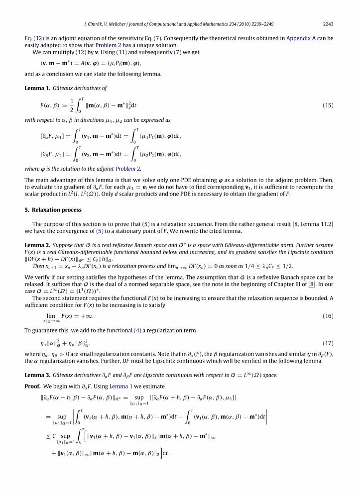
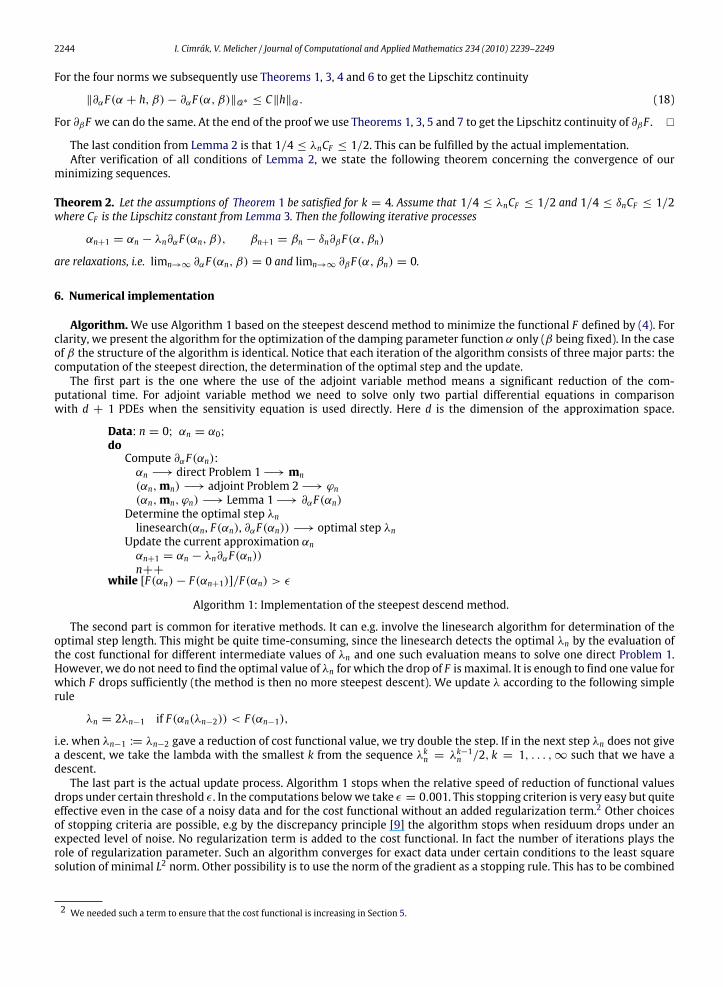
Fig. 1. Determination of the smooth damping parameter. The exact solution and the reconstructions with different noise levels of 0%, 1% and 10%.

exact 0% 1% 10%

Fig. 2. Determination of piecewise constant damping parameter. The exact solution and the reconstructions with different noise levels of 0%, 1% and 10%.

with addition of some regularization term to the cost functional in the noisy case. Different choices are possible, e.g. totalvariation regularization which preserves sharp edges. For regularization of inverse problem see e.g. [10].

Approximation. To solve the direct Problem 1, we employ the method developed in [11], where the convergence and theerror estimates of time discretization are proved. This method is based on the variational formulation of (3), so the standardW 1,2(Ω)-conforming finite elements are used to discretize in space.The magnetization preserves length |m| = 1. The above mentioned method preserves the length of the magnetization

only asymptotically. Therefore we project the magnetization to keep the constant length and to stabilize the method.As explained in Section 4, the adjoint problem is a linear parabolic PDE. Thus we also use the standard W 1,2(Ω)-

conforming finite element formulation. The simple implicit Backward Euler approximation of the time derivative is used.For numerical realization, we used FreeFem++ package [12].

Test with smooth exact solution α. The first numerical test was run with the following continuous exact solution

αexact = 0.02+ 0.01 sin(π2xy), (x, y) ∈ (0, 1)2.

The precession factor β was fixed to 0.1. All the finite element functions were defined on a regular mesh with diameterh = 1/30, i.e. the dimension of the approximation space was d = 961. The time step of numerical schemes was τ = 0.01and T = 15τ . The reconstruction of the exact profile depicted in Fig. 1 for measurements without noise was almost perfect.When we added noise of the level 1%, the reconstruction became worse but still acceptable. Increasing the noise to 10%resulted in the loss of almost any information.

Test with discontinuous exact solution α. Next numerical test was run with a discontinuous piecewise constant solution hav-ing 4 different values 0.005, 0.01, 0.02 and 0.03 in Ω = (0, 1)2. The other parameters were again h = 1/30, τ = 0.01and T = 15τ . The profile is depicted in Fig. 2. We see that already the reconstruction of the exact profile was not so suc-cessful as for the case of the smooth exact solution. The explanation is in the regularization that has been used. The L2-regularization [10] introduced by algorithm causes a smoothing effect that is harmless in the case of the exact solution butdestroys the information about sharp edges in the case of the discontinuous exact solution. When we added noise of thelevel 1%, we see that the reconstruction became almost unacceptable.

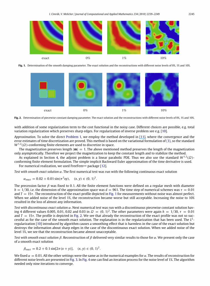
Test with smooth exact solution β . Reconstruction of β delivered very similar results to those for α. We present only the caseof a smooth exact solution

βexact = 0.2+ 0.1 sin[2π(x+ y)], (x, y) ∈ (0, 1)2.

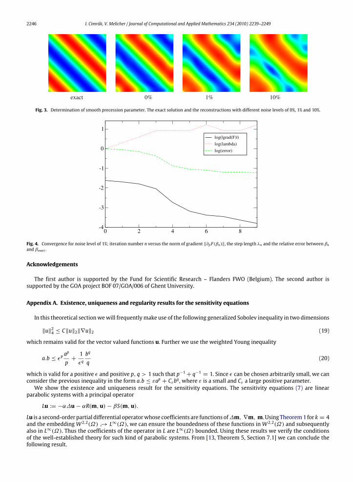
We fixed α = 0.01. All the other settings were the same as in the numerical examples for α. The results of reconstruction fordifferent noise levels are presented in Fig. 3. In Fig. 4 one can find an iteration process for the noise level of 1%. The algorithmneeded only nine iterations to converge.

2246 I. Cimrák, V. Melicher / Journal of Computational and Applied Mathematics 234 (2010) 2239–2249

exact 0% 1% 10%

Fig. 3. Determination of smooth precession parameter. The exact solution and the reconstructions with different noise levels of 0%, 1% and 10%.

0 2 4 6 8-4

-3

-2

-1

0

1log(|grad(F)|)

log(lambda)

log(error)

Fig. 4. Convergence for noise level of 1%; iteration number n versus the norm of gradient ‖∂βF(βn)‖, the step length λn and the relative error between βnand βexact .

Acknowledgements

The first author is supported by the Fund for Scientific Research – Flanders FWO (Belgium). The second author issupported by the GOA project BOF 07/GOA/006 of Ghent University.

Appendix A. Existence, uniqueness and regularity results for the sensitivity equations

In this theoretical sectionwewill frequentlymake use of the following generalized Sobolev inequality in two dimensions

‖u‖24 ≤ C‖u‖2‖∇u‖2 (19)

which remains valid for the vector valued functions u. Further we use the weighted Young inequality

a.b ≤ εpap

p+1εq

bq

q(20)

which is valid for a positive ε and positive p, q > 1 such that p−1+ q−1 = 1. Since ε can be chosen arbitrarily small, we canconsider the previous inequality in the form a.b ≤ εap + Cεbq, where ε is a small and Cε a large positive parameter.We show the existence and uniqueness result for the sensitivity equations. The sensitivity equations (7) are linear

parabolic systems with a principal operator

Lu := −α∆u− αR(m,u)− βS(m,u).

Lu is a second-order partial differential operatorwhose coefficients are functions of∆m, ∇m, m. Using Theorem1 for k = 4and the embeddingW 2,2(Ω) → L∞(Ω), we can ensure the boundedness of these functions inW 2,2(Ω) and subsequentlyalso in L∞(Ω). Thus the coefficients of the operator in L are L∞(Ω) bounded. Using these results we verify the conditionsof the well-established theory for such kind of parabolic systems. From [13, Theorem 5, Section 7.1] we can conclude thefollowing result.

I. Cimrák, V. Melicher / Journal of Computational and Applied Mathematics 234 (2010) 2239–2249 2247

Theorem 3. Let the assumptions of Theorem 1 be satisfied for k = 4. Then there exist a unique solution vi to the sensitivityequation (7) for i = 1, 2 respectively satisfying

ess supt∈I(‖vi‖W2,2 + ‖∂tvi‖2)+

[∫ T

0‖∂tvi‖2W1,2

] 12

≤ C‖µi‖∞. (21)

Appendix B. Stability of the direct problem

The α-stability. Take two functions α1 and α2 and supposemi are solutions to Problem 1 for function αi, i = 1, 2 withthe same initial condition. Then the differencem := m1 −m2 obeys the following equation

∂tm− α2∆m = (α1 − α2)P1(m1)+ α2[〈∇m,∇m1 +∇m2〉m1 + |∇m2|2m

]−β

[m×∆m1 +m2 ×∆m

], (22)

with zero initial condition. This equation has basically the same structure as the sensitivity equation; the principal operatorof (22) is slightly different. Nevertheless we can again verify the assumptions for [13, Theorem 5, Section 7.1] and thus wecan derive an analogical result stated in the following theorem.

Theorem 4. Let the assumptions of Theorem 1 be satisfied for k = 4. For an arbitrary αi ∈ L∞(Ω), i = 1, 2 considerProblem 1i derived from Problem 1 simply by replacing α with αi and denote bymi the solution to Problem 1i. Then the differencem := m1 −m2 enjoys

ess supt∈I(‖m‖W2,2 + ‖∂tm‖2)+

[∫ T

0‖∂tm‖2W1,2

] 12

≤ C(‖α1 − α2‖∞).

The β-stability. Similarly as before, take two functions β1 and β2 and suppose mi are solutions to Problem 1 for functionβ i, i = 1, 2 with the same initial condition. Then for the differencem = m1 −m2 we can write

∂tm− α∆m = (β1 − β2)P2(m1)+ α[〈∇m,∇m1 +∇m2〉m1 + |∇m2|2m

]−β2

[m×∆m1 +m2 ×∆m

], (23)

with the zero initial condition. Again, the equation has the same structure as the sensitivity equation. Thus an analogicalresult is stated in the following theorem.

Theorem 5. Let the assumptions of Theorem 1 be satisfied for k = 4. For an arbitrary β i ∈ L∞(Ω), i = 1, 2 considerProblem 1i derived from Problem 1 simply by replacing β with β i and denote bymi the solution to Problem 1i. Then the differencem := m1 −m2 enjoys

ess supt∈I(‖m‖W2,2 + ‖∂tm‖2)+

[∫ T

0‖∂tm‖2W1,2

] 12

≤ C(‖β1 − β2‖∞).

Appendix C. Stability of the sensitivity equations

The α-stability. Take two functions α1, α2 and suppose m1, m2 are the corresponding solutions to Problem 1 withthe same initial condition (IC), respectively. Suppose vi1 are solutions to the first sensitivity equation (7) where functionα = αi, i = 1, 2 with the same IC. Then the difference v1 := v11 − v21 obeys

∂tv1 − α2∆v1 − α2R(m2, v1)− βS(m2, v1) = (α1 − α2)[R(m1, v11)+∆v11 + µ1P1(m

1)]

+α2[R(m1, v11)− R(m

2, v11)]+ β

[S(m1, v11)− S(m

2, v11)]+ α2µ1

[P1(m1)− P1(m2)

]. (24)

We have again obtained a system similar to (7) with the same principal operator and a slightly different right-hand sideconsisting of four terms denoted by A1, A2, A3, A4, respectively. Suppose the assumptions of Theorem 1 are satisfied fork = 4. Then, using the embeddingW 2,2(Ω) → L∞(Ω) we can estimatemi,∇mi and ∆mi in L∞(ΩT ) by some constant C

2248 I. Cimrák, V. Melicher / Journal of Computational and Applied Mathematics 234 (2010) 2239–2249

for i = 1, 2. Further from Theorem 3 we have directly boundedness of vi1 in L∞(I,W 2,2(Ω)) again for i = 1, 2. Using these

preliminaries we can estimate terms A1, A2, A3, A4 in the following way. For an arbitrary t we can conclude that

‖A1‖2 =∥∥(α1 − α2)[R(m1, v11)+∆v11 + µ1P1(m

1)]∥∥2

≤ C‖α1 − α2‖∞[‖m1‖∞ + ‖∇m1‖∞ + ‖∆m1‖∞](‖v11‖W2,2 + ‖µ1‖∞) ≤ C‖α1− α2‖∞‖µ1‖∞,

using Theorem 3 at the end. For term A2 we can write

‖A2‖2 =∥∥α2[R(m1, v11)− R(m2, v11)]∥∥2

≤ ‖α2‖∞

[2‖〈∇v11,∇m〉m

1‖2 + 2‖〈∇v11,∇m

2〉m‖2 + ‖〈∇m,∇m1〉v11‖2 + ‖〈∇m

2,m〉v11‖2]

≤ C[‖∇v11‖4‖∇m‖4 + ‖∇v

11‖4‖m‖4 + ‖∇m‖4‖v

11‖4 + ‖m‖4‖v

11‖4

].

Using the embeddingsW 2,2(Ω) → W 1,4(Ω) andW 2,2(Ω) → L∞(Ω) we go further, and again using Theorems 3 and 4,we arrive at

‖A2‖2 ≤ C‖v11‖W2,2‖m‖W2,2 ≤ C‖µ1‖∞‖α1− α2‖∞.

For term A3 we have a similar result, again using Theorems 3 and 4 at the end

‖A3‖2 =∥∥β[S(m1, v11)− S(m2, v11)]∥∥2 ≤ ‖β‖∞[‖m×∆v11‖2 + ‖v

11 ×∆m‖2

]≤ C

[‖m‖∞‖∆v11‖2 + ‖v

11‖∞‖∆m‖2

]≤ C‖v11‖W2,2‖m‖W2,2 ≤ C‖µ1‖∞‖α

1− α2‖∞.

Finally for term A4 we get

‖A4‖2 =∥∥α2µ1[P1(m1)− P1(m2)]∥∥2

≤ C‖µ1‖∞[‖∆m‖2 + ‖〈∇m,∇m1 +∇m2〉m1‖2 + ‖|∇m2|2m‖2

]≤ C‖µ1‖∞‖m‖W2,2 ≤ C‖µ1‖∞‖α

1− α2‖∞,

where we have used Theorem 4 at the end.Summarizing the previous four estimates we succeed in estimating the right-hand side of (24) in the norm of the space

L∞(I, L2(Ω)) by C‖µ1‖∞‖α1 − α2‖∞. This again allows for the application of [13, Theorem 5, Section 7.1] for the solutionto (24). We state this result in the following theorem.

Theorem 6. Let the assumptions of Theorem 1 be satisfied for k = 4. For an arbitrary αi ∈ L∞(Ω), i = 1, 2 consider Problem 1iderived from Problem 1 simply by replacing α with αi and denote bymi their solutions. Further consider two sensitivity equationswith respect to α corresponding to Problem 1i and denote by vi1 their solutions, i = 1, 2. Then the difference v1 := v11− v21 enjoys

ess supt∈I‖v1‖W1,2 +

[∫ T

0‖v1‖2W2,2

] 12

+

[∫ T

0‖∂tv1‖22

] 12

≤ C‖µ1‖∞‖α1 − α2‖∞.

The β-stability. The stability of the sensitivity equation on β can be obtained repeating all the steps from the section. Wepresent the resulting theorem only.

Theorem 7. Let the assumptions of Theorem 1 be satisfied for k = 4. For an arbitrary β i ∈ L∞(Ω), i = 1, 2 consider Problem 1iderived from Problem 1 simply by replacing β with β i and denote bymi their solutions. Further consider two sensitivity equationswith respect to β corresponding to Problem 1i and denote by vi2 their solutions, i = 1, 2. Then the difference v2 := v12− v22 enjoys

ess supt∈I‖v2‖W1,2 +

[∫ T

0‖v2‖2W2,2

] 12

+

[∫ T

0‖∂tv2‖22

] 12

≤ C‖µ2‖∞‖β1 − β2‖∞.

References

[1] I. Cimrák, V. Melicher, The Landau–Lifshitz model for shape optimization of MRAMmemories, PAMM 6 (1) (2006) 23–26.[2] I. Cimrák, V. Melicher, Sensitivity analysis framework for micromagnetism with application to optimal shape design of MRAM memories, InverseProblems 23 (2007) 563–588.

[3] G. Bertotti, Hysteresis in Magnetism, Academic Press, 1998.[4] I. Cimrák, A survey on the numerics and computations for the Landau–Lifshitz equation of micromagnetism, Arch. Comput. Methods Engrg. 15 (3)(2008) 277–309.

[5] L’. Baňas, A. Prohl, M. Slodička, Modeling of thermally assisted magnetodynamic, SIAM J. Numer. Anal. 47 (1) (2008) 551–574.[6] A. Prohl, Computational Micromagnetism, in: Advances in Numerical Mathematics, B.G. Teubner, Stuttgart, 2001.

I. Cimrák, V. Melicher / Journal of Computational and Applied Mathematics 234 (2010) 2239–2249 2249

[7] G. Carbou, P. Fabrie, Regular solutions for Landau–Lifshitz equation in a bounded domain, Differential Integral Equations 14 (2) (2001) 213–229.[8] M.M. Vainberg, Variational Method and Method of Monotone Operators in the Theory of Nonlinear Equations, JohnWiley & Sons, New York, Toronto,1973.

[9] V.A. Morozov, On the solution of functional equations by the method of regularization, Doklady Akad. Nauk SSSR 7 (1966) 414–417 (in Russian).[10] H.W. Engl, M. Hanke, A. Neubauer, Regularization of Inverse Problems, in: Mathematics and its Applications, vol. 375, Kluwer Academic Publishers,

Dordrecht, 1996.[11] I. Cimrák, Error estimates for a semi-implicit numerical scheme solving the Landau–Lifshitz equation with an exchange field, IMA J. Numer. Anal. 25

(2005) 611–634.[12] O. Pironneau, F. Hecht, A. Le Hyaric, Freefem++ package. http://www.freefem.org.[13] L. Evans, Partial Differential Equations, in: Graduate Studies in Mathematics, vol. 19, American Mathematical Society, Providence, RI, 1998.