arX

iv:m

ath-

ph/0

3050

49v1

23

May

200

3

Transport and Dissipation in Quantum Pumps

J. E. Avron ∗, A. Elgart †, G.M. Graf ‡and L. Sadun §

February 7, 2008

Abstract

This paper is about adiabatic transport in quantum pumps. The notion of “energy shift”, a

self-adjoint operator dual to the Wigner time delay, plays a role in our approach: It determines

the current, the dissipation, the noise and the entropy currents in quantum pumps. We discuss

the geometric and topological content of adiabatic transport and show that the mechanism of

Thouless and Niu for quantized transport via Chern numbers cannot be realized in quantum

pumps where Chern numbers necessarily vanish.

Contents

1 Introduction 2

2 Pedestrian derivation of BPT 4

2.1 The two channels case . . . . . . . . . . . . . . . . . . . . . . . . . . . . . . . . . . 52.2 The snowplow . . . . . . . . . . . . . . . . . . . . . . . . . . . . . . . . . . . . . . . 52.3 The battery . . . . . . . . . . . . . . . . . . . . . . . . . . . . . . . . . . . . . . . . 62.4 The sink . . . . . . . . . . . . . . . . . . . . . . . . . . . . . . . . . . . . . . . . . . 72.5 The ineffective variable . . . . . . . . . . . . . . . . . . . . . . . . . . . . . . . . . . 7

3 Alternative perspectives on BPT 8

3.1 An axiomatic derivation . . . . . . . . . . . . . . . . . . . . . . . . . . . . . . . . . 83.2 Classical pumps . . . . . . . . . . . . . . . . . . . . . . . . . . . . . . . . . . . . . . 103.3 Currents and the T -E uncertainty . . . . . . . . . . . . . . . . . . . . . . . . . . . 12

4 Time dependent scattering and Weyl calculus 14

4.1 The energy shift . . . . . . . . . . . . . . . . . . . . . . . . . . . . . . . . . . . . . 144.2 The Weyl calculus . . . . . . . . . . . . . . . . . . . . . . . . . . . . . . . . . . . . 15

5 Adiabatic transport 15

5.1 Adiabatic scattering . . . . . . . . . . . . . . . . . . . . . . . . . . . . . . . . . . . 165.2 Currents . . . . . . . . . . . . . . . . . . . . . . . . . . . . . . . . . . . . . . . . . . 165.3 Dissipation . . . . . . . . . . . . . . . . . . . . . . . . . . . . . . . . . . . . . . . . 175.4 Entropy and noise currents . . . . . . . . . . . . . . . . . . . . . . . . . . . . . . . 18

6 Examples 19

6.1 The bicycle pump . . . . . . . . . . . . . . . . . . . . . . . . . . . . . . . . . . . . . 196.2 The U-turn pump . . . . . . . . . . . . . . . . . . . . . . . . . . . . . . . . . . . . . 206.3 A family of optimal pumps . . . . . . . . . . . . . . . . . . . . . . . . . . . . . . . 216.4 The phase space of a snowplow . . . . . . . . . . . . . . . . . . . . . . . . . . . . . 226.5 Classical scattering from a battery . . . . . . . . . . . . . . . . . . . . . . . . . . . 23

∗Department of Physics, Technion, 32000 Haifa, Israel†Courant Institute of Mathematical Sciences, New York, NY 10012, USA‡Theoretische Physik, ETH-Honggerberg, 8093 Zurich, Switzerland§Department of Mathematics, University of Texas, Austin Texas 78712, USA

1

7 Geometry and topology 23

7.1 Charge transport and Berry’s phase . . . . . . . . . . . . . . . . . . . . . . . . . . 247.2 Global angle . . . . . . . . . . . . . . . . . . . . . . . . . . . . . . . . . . . . . . . . 257.3 Curvature . . . . . . . . . . . . . . . . . . . . . . . . . . . . . . . . . . . . . . . . . 257.4 The two channel case . . . . . . . . . . . . . . . . . . . . . . . . . . . . . . . . . . . 267.5 Chern and winding numbers . . . . . . . . . . . . . . . . . . . . . . . . . . . . . . . 267.6 Geometry of dissipation and noise . . . . . . . . . . . . . . . . . . . . . . . . . . . 27

A Comparison with the theory of full counting statistics 28

A.1 The Lesovik-Levitov formula . . . . . . . . . . . . . . . . . . . . . . . . . . . . . . 28A.2 Charge transport . . . . . . . . . . . . . . . . . . . . . . . . . . . . . . . . . . . . . 28A.3 Splitting the noise . . . . . . . . . . . . . . . . . . . . . . . . . . . . . . . . . . . . 29A.4 Thermal noise . . . . . . . . . . . . . . . . . . . . . . . . . . . . . . . . . . . . . . . 29A.5 Shot noise at finite temperatures . . . . . . . . . . . . . . . . . . . . . . . . . . . . 29A.6 Shot noise at T = 0 . . . . . . . . . . . . . . . . . . . . . . . . . . . . . . . . . . . . 30

1 Introduction

An adiabatic quantum pump [33] is a time-dependent scatterer connected to several leads. Fig. 1is an example with two leads. Each lead may have several channels. The total number of channels,in all leads, will be denoted by n. Each channel is represented by a semi-infinite, one dimensional,(single mode) ideal wire. We assume that the particles propagating in the channels are non-interacting1 and all have dispersion ǫ(k). For the sake of concreteness we shall take quadraticdispersion, ǫ(k) = k2/2, but most of our results carry over to more general dispersions. We alsoassume that the incoming particles are described by a density matrix ρ common to all channels:ρ(E) = (1 + eβ(E−µ))−1, with chemical potential µ and temperature T . The scatterer is adiabaticwhen its characteristic frequency ω ≪ 1/τ , with τ a the typical dwell time in the scatterer. Wetake units so that kB = ~ = m = e = +1.

An incoming particle sees a quasi-static scatterer. The scattering can therefore be computed,to leading order, by time-independent quantum mechanics, using the scattering Hamiltonian ineffect at the time that the particle reaches the scatterer. In other words, we pretend that theHamiltonian always was, and always will be, the Hamiltonian seen by the particle at the time ofpassage. This gives the “frozen S-matrix”. Since time-independent systems conserve energy, sodoes the frozen S-matrix. We denote by S(E, t) the on-shell frozen S-matrix.

The outgoing states have, to order ω0, the same occupation density as the incoming states(since S(E, t) is a unitary n× n matrix and the incoming densities are the same for all channels).This implies no net transport. However, at order ω, there is an interesting interference effect: Anincoming particle of well-defined energy does not have a well-defined time of passage. This spreadin time is a consequence of the uncertainty principle, and is not related to the dwell time of theparticle in the scatterer. Thus, even if ω ≪ 1/τ , the (frozen) S-matrix seen by the tail of thewave packet will differ slightly from that seen by the head of the wave packet. This differentialscattering causes the outgoing occupation densities to differ from the incoming densities to orderω1, leading to a nonzero transport.

The density matrix for the outgoing states, ρout, is determined by ρ(H0), the density matrixof the incoming states, and the S-matrix. Let Sd be the exact (dynamical) S-matrix. As we shallexplain in section 5, ρout is given by

ρout = ρ(H0 − Ed), Ed = i SdS∗d . (1.1)

A dot denotes derivative with respect to time2. Ed is the operator of energy shift introduced in[24]. It combines information on the state of the scatterer with its rate of change Sd. For time

1Quantum pumps have also been discussed in the context of Luttinger liquids, see e.g. [2, 30].2The time dependence of Sd is discussed in section 5.

2

Figure 1: A model of a quantum scatterer with two leads.

independent scattering, Ed = 0 and Eq. (1.1) is an expression of conservation of energy. Theformula for ρout, Eq. (1.1), holds independently of whether the scattering is adiabatic or not.

We call the frozen analog of the operator Ed the matrix of energy shift. It is the n× n matrix

E(E, t) = i S(E, t)S∗(E, t), (1.2)

and is a natural dual to the more familiar Wigner time delay [15]

T (E, t) = −i S′(E, t)S∗(E, t). (1.3)

where prime denotes derivative with respect to E. As we shall see in section 7.3 their commutator

Ω = i[T , E ] (1.4)

has a geometric interpretation of a curvature in the time-energy plane, analogous to the adiabaticcurvature.

Adiabatic transport can be expressed in terms of the matrix of energy shift. For example, theBPT [13] formula for the expectation value of the current in the j-th channel, 〈Q〉j takes the form:

〈Q〉j(t) = − 1

2π

∫ ∞

0

dE ρ′(E) Ejj(E, t). (1.5)

At T = 0, −ρ′ is a delta function at the Fermi energy and the charge transport is determined bythe energy shift at the Fermi energy alone.

There are two noteworthy aspects of this formula. The first one is that 〈Q〉, which is of orderω, can be accurately computed from frozen scattering data which is only an ω0 approximation.The second one is that the formula holds all the way to T = 0, where the adiabatic energy scale ωis large compared to the energy scale T .

The energy shift also determines certain transport properties that are of order ω2. An exampleis dissipation at low temperatures. Let 〈E〉j(t) be the expectation value of energy current in thej-th channel. Part of the energy is forever lost as the electrons are dumped into the reservoir. Thepart that can be recovered from the reservoir, by reclaiming the transported charge, is µ〈Q〉j(t).We therefore define the dissipation in a quantum channel as the difference of the two. As we shallshow in section 5.3 the dissipation at T = 0 is3:

〈E〉j(t) − µ〈Q〉j(t) =1

4π

(

E2)

jj(µ, t) ≥ 0. (1.6)

Both the dissipation and the current admit transport formulas that are local in time at T = 0.Namely, the response at time t is determined by the energy shift at the same time. This isremarkable for at T = 0 quantum correlations decay slowly in time and one may worry thattransport at time t will retain memory about the scatterer at early times. This brings us totransport equations which admit a local description only at finite temperatures.

The entropy and noise currents are defined as the difference between the outgoing (into thereservoirs) and incoming entropy (or noise) currents. Namely,

sj(t, µ, T ) = s(ρout,j) − s(ρj), s(ρ) =1

2π

∫

dE (h ρ)(E, t) (1.7)

3For related results on dissipation see e.g. [25]. For relations between dissipation and the S-matrix see [1]

3

where [18, 12]

h(x) =

−x log x− (1 − x) log(1 − x) entropy,

x(1 − x) noise.(1.8)

In the adiabatic limit, ω → 0, and for ω ≪ T ≪√

ω/τ we find (see section 5.4)

sj(t, µ, T ) =β

2πk∆E2

j (µ, t) ≥ 0, k =

2 entropy;

6 noise,(1.9)

where∆E2

j =(

E2)

jj−

(

Ejj

)2. (1.10)

When T . ω the entropy and noise currents at time t are mindful of the scattering data for earliertimes and there are no transport equations that are local in time. What sets them apart from thecurrent and the dissipation is the non-linear dependence on the density. The non-linearity makesthe transport sensitive to the slow decay of correlations.

Our result about the noise overlap with results that follow from the “full counting statistics”of Levitov et. al. [21]. When there is overlap, the results agree. However, the results are mostlycomplementary, a reflection of the fact that both the questions and the methods are different.“Counting statistics” determine transport in a pump cycle in terms of the entire history of thepump. We give information that is local in time. In this sense, we give stronger results. On theother hand, the counting statistics determine all moments all the way down to zero temperature,while our results go down to T = 0 for the current and dissipation but not for the entropy and noise.A detailed comparison of our results with results that follow from the Lesovik-Levitov formalism[21] is made in appendix A. For other results on noise in pumps see e.g., [27].

Transport in adiabatic scattering is conveniently described using semi-classical methods [22]a.k.a. pseudo-differential (Weyl) calculus [28]. As we shall explain in section 5, S(E, t) is theprincipal symbol of the exact S-matrix, Sd. Semi-classical methods can be used to derive Eqs. (1.5,1.6, 1.7). For an alternate point of view using coherent states see [8].

In section 7 we discuss the geometric and topological significance of our results. We shall seethat charge transport can be formulated in terms of the curvature, or Chern character, of a naturalline bundle. This is reminiscent of works of Thouless and Niu [34] which identified quantized chargetransport with Chern numbers [35] and inspired the study of quantum pumps. Nevertheless thesituation is different here, since the bundle is trivial and, besides, the integration manifold hasa boundary. This does not preclude the possibility that charge is quantized for reasons otherthan being a Chern number. In fact, one can geometrically characterize a class of periodic pumpoperations [7] for which the transported charge in a cycle, and not just its expectation value, is anon-random integer. It is to be cautioned that a small change of the scattering matrix will typicallydestroy this quantization.

2 Pedestrian derivation of BPT

At T = 0 the Fermi energy is a step function and ρ′(E) = −δ(µ− E), and BPT, Eq. (1.5), takesthe form

〈Q〉j(µ, t) =1

2πEjj(µ, t). (2.1)

In this section we shall describe an argument [6] that explains this equation in the two channel case.The two channel case is special in that the changes in the scattering matrix break into elementaryprocesses so that for each one BPT follows either from simple physical arguments or from knownfacts4.

4We assume that the transported charge depends only on S(µ) and, linearly, on dS(µ), regardless of the physicalrealization of the scatterer.

4

2.1 The two channels case

In the two channel case, Fig. 1, the frozen, on shell, S-matrix takes the form

S(µ) =

(

r t′

t r′

)

(µ), (2.2)

with r and t (respectively r′ and t′) the reflection and transmission coefficients from the left (right).Eq. (2.1) reads

2π 〈dQ〉− = i(rdr + t′dt′), 2π 〈dQ〉+ = i(r′dr′ + tdt) (2.3)

〈dQ〉− is made from data (r, t′) describing the scattering to the left, and similarly 〈dQ〉+ fromthose to the right5.

To identify the physical interpretation of the differentials we introduce new coordinates (θ, α, φ, γ).The most general unitary 2 × 2 matrix can be expressed in the form:

S = eiγ

(

eiα cos θ ie−iφ sin θieiφ sin θ e−iα cos θ

)

(2.4)

where 0 ≤ α, φ < 2π, 0 ≤ γ < π and 0 ≤ θ ≤ π/2. In terms of these parameters, the BPT formulareads

2π 〈dQ〉± = ±(

cos2 θ)

dα∓(

sin2 θ)

dφ− dγ. (2.5)

As we shall now explain, the variations dα, dφ and dγ can be identified with simple physicalprocesses.

2.2 The snowplow

ξd

Figure 2: Moving the scatterer changes α→ α+ 2kF dξ

Let kF be the Fermi momentum associated with µ. Translating the scatterer a distance dξmultiplies r, (r′) by e2ikF dξ, (e−2ikF dξ), and leaves t and t′ unchanged. It follows that dα = 2kFdξcorresponds to shifting the scatterer.

As the scatterer moves, it attempts to push the kF dξ/π = dα/2π electrons that occupy theregion of size dξ out of the way, much as a snowplow attempts to clear a path on a winter day.Of these, a fraction |t|2 = sin2 θ will pass through the scatterer (or rather, the scatterer will pass

through them), while the remaining fraction |r|2 = cos2 θ will be propelled forward, resulting innet charge transport of

2π 〈dQ〉± = ±(

cos2 θ)

dα, (2.6)

in accordance with Eq. (2.5).

Remark 2.1 It is instructive to examine the special case of a uniformly moving scatterer wherewe can use Galilei transformations to compute the charge transport exactly. By taking the limit ofslowly moving scatterer we get a check on the result above.

Since the mass of the electron is one, the Galilean shift from the lab frame to the frame of thescatterer shifts each momentum by −ξ. In the lab frame, the incoming states are filled up to theFermi momentum kF while in the moving frame the incoming states of the ± channels are filledup to momenta kF ± ξ. In the moving frame, the outgoing states on the ± channels are filled up

5This is why S∗ is on the right in the energy shift, Eq. (1.2).

5

to kF ∓ ξ, and partially filled with density |t′(k)|2 for momenta in the interval (kF − ξ, kF + ξ).Transforming back to the lab frame we find for δρ of the − (=left) channel

δρ−(k2) =

0 if k < kF − 2ξ

−|r′(k + ξ)|2 if kF − 2ξ < k < kF

0 if k > kF .

(2.7)

To order ξ,δρ−(E) = −2kF ξ |r′(kF )|2δ(E − µ). (2.8)

Since the current is

〈Q〉j(t) =1

2π

∫ ∞

0

dE δρj(E, t), (2.9)

Eq. (2.6) is reproduced.

Remark 2.2 The net outflow of charge, 〈dQ〉− + 〈dQ〉+, vanishes to order ξ but not to order ξ2.This is because the moving snowplow leaves a region of reduced density in its wake.

2.3 The battery

A(x,t)

Figure 3: Applying a vector potential changes φ→ φ+∫

A

To vary φ we add a vector potential A. This induces a phase shift dφ =∫

A across the scatterer,and multiplies t, (t′) by eidφ, (e−idφ), while leaving r and r′ unchanged. This phase shift dependsonly on

∫

A, and is independent of the placement or form of the vector potential. The variation in

the vector potential induces an EMF of strength −∫

A = −φ. To first order, the current is simply

the voltage times the Landauer conductance |t|2/2π [18]. That is,

2π 〈dQ〉± = ∓(

sin2 θ)

dφ. (2.10)

in agreement with Eq. (2.5).

Remark 2.3 Consider the special case of a time independent voltage drop. In a gauge where thebattery is represented by a scalar potential, the pump is represented by a time independent scatteringproblem where the potential has slightly different asymptotes at ±∞. If the battery is placed to theleft of the scatterer, the states of particles incident from that side are occupied up to energy µ− φ,while those incident from the right are occupied up to energy µ. Suppose φ is negative. Then δρ+

is

δρ+(E) =

0 if E < µ,

|t(E)|2 if µ < E < µ− φ ,

0 if E > µ− φ

(2.11)

If, however, the battery is placed to the right of the scatterer then δρ+ is

δρ+(E) =

0 if E < µ,

|t(E + φ)|2 if µ < E < µ− φ ,

0 if E > µ− φ

(2.12)

6

In either case, to leading order in φ,

δρ+(E) = −φ |t(µ)|2δ(E − µ). (2.13)

Plugging in Eq. (2.9), we recover Eq. (2.5).

Remark 2.4 To leading order in φ, δρ+ is independent of whether the battery is to the left ofthe pump or to the right of it. To order φ2 this is no longer true as one sees from Eq. (2.11,2.12). The frozen S-matrix is, however, insensitive to the location of the battery. It follows thatit is impossible to have a formula for δρ, accurate to order O(ω2), that involves only the frozenS-matrix and its derivatives (see [26] for some model calculations in the non-adiabatic regime).

2.4 The sink

The scattering matrix depends on a choice of fiducial points: The choice of an origin for the twochannels. Moving the two fiducial points out a distance dξ may be interpreted as forfeiting partof the channels in favor of the scatterer. This new, bigger, scatterer is shown schematically in Fig.4. This transforms the scattering matrix according to

S(kF ) → eidγ S(kF ), dγ = 2kFdξ. (2.14)

This operation removes kF dξ/π electrons from each channel and so we get

2π 〈dQ〉± = −2kFdξ = −dγ, (2.15)

in accordance with Eq. (2.5). Changing γ is therefore equivalent to having the pump swallowparticles from the reservoirs.

ξd

Figure 4: A scatterer that has gobbled up dξ of each wire.

For arbitrary variations dS the above result still holds for the sum dQ− + dQ+. This followsdirectly from a fact in scattering theory known as Birman-Krein formula [36] and in physics asFriedel sum rule [16] which says that the excess number of states below energy µ associated withthe scatterer is (2πi)−1 log detS(µ), whence

−2π(

〈dQ〉− + 〈dQ〉+)

(µ) = −id log detS(µ) = 2dγ. (2.16)

2.5 The ineffective variable

We have already seen that changes in α, φ, γ yield transported charges dQ± which are correctlyreproduced by Eq. (2.5). Moreover, for any change of s, the sum 〈dQ〉− + 〈dQ〉+ is, too. Tocomplete the derivation of Eq. (2.5) we must consider variations in θ, with α, φ and γ fixed, andshow that 〈dQ〉− − 〈dQ〉+ = 0.

Suppose a scatterer has α, φ and γ fixed, but θ changes with time. By adding a (fixed!) vectorpotential and translating the system a (fixed!) distance6, we can assume that α = φ = 0. Now

6This can be achieved, in general, only at a fixed energy, and we pick the energy to be the Fermi energy µ.

7

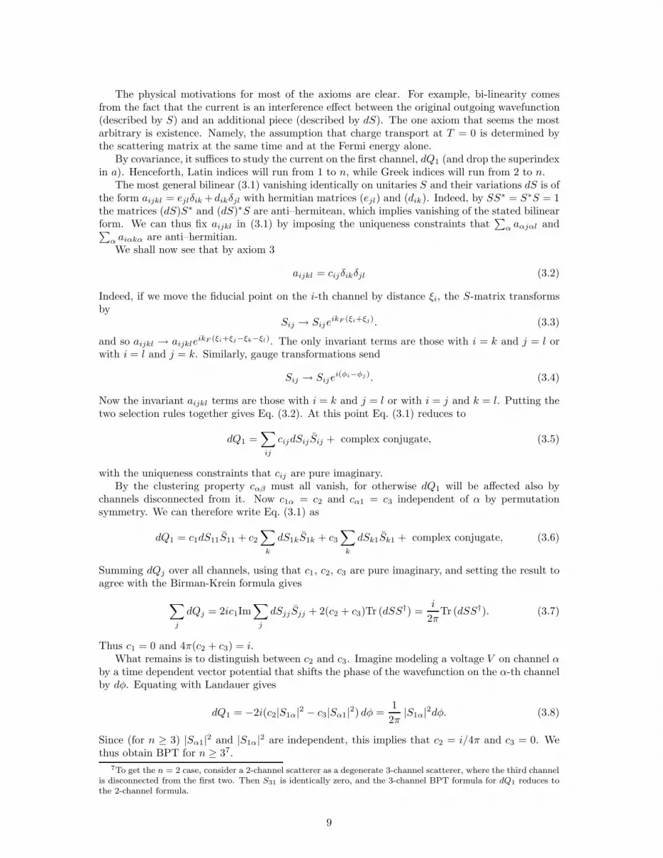
imagine a second scatterer that is the mirror image of the first (i.e., with right and left reversed)as in Fig. 5. Since θ and γ are invariant under right-left reflection, and since α and φ are oddunder right-left reflection, the second scatterer has the same frozen S matrix as the first, and thisequality persists for all time.

Figure 5: An asymmetric scatterer and its image under reflection

¿From the frozen scattering data we therefore conclude that the currents for the second systemare the same as for the first. However, by reflection symmetry, 〈dQ〉− −〈dQ〉+ for the first systemequals 〈dQ〉+ − 〈dQ〉− for the second. We conclude that 〈dQ〉+ − 〈dQ〉− = 0 for variations of θ.

3 Alternative perspectives on BPT

The pedestrian argument does not extend beyond the two channel case. This is because withmore than two channels, a general variation dS cannot be described in terms of known physicalprocesses. One can, nevertheless, derive BPT from general and simple physical considerations,without recourse to formal perturbation expansions in scattering theory.

3.1 An axiomatic derivation

The BPT formula for the current follows from the following natural axioms:

1. Existence and Bilinearity:

dQm =∑

ijkl

amijkldSijSkl + complex conjugate, (3.1)

with universal (complex) coefficients amijkl .

2. Covariance: The formula is covariant under permutation of the channels. In particular, it isinvariant under permutations of the channels other than the m-th.

3. Gauge invariance: The formula is unchanged by time-independent gauge transformations,and also under time-independent changes in the fiducial points.

4. Cluster: If the system consists of two subsystems, disconnected from one another, thenthe currents in each subsystem depend only on the part of the S matrix that governs thatsubsystem.

5. Landauer: If a voltage, applied to a single lead m′ 6= m, is modeled by a time-dependentgauge transformation, then dQm is given by the Landauer formula where the transmissionprobability is given by the scattering probability m′ → m.

6. Birman-Krein:∑

j

dQj =i

2πd log(detS) =

i

2πTr (dSS†).

8

The physical motivations for most of the axioms are clear. For example, bi-linearity comesfrom the fact that the current is an interference effect between the original outgoing wavefunction(described by S) and an additional piece (described by dS). The one axiom that seems the mostarbitrary is existence. Namely, the assumption that charge transport at T = 0 is determined bythe scattering matrix at the same time and at the Fermi energy alone.

By covariance, it suffices to study the current on the first channel, dQ1 (and drop the superindexin a). Henceforth, Latin indices will run from 1 to n, while Greek indices will run from 2 to n.

The most general bilinear (3.1) vanishing identically on unitaries S and their variations dS is ofthe form aijkl = ejlδik +dikδjl with hermitian matrices (ejl) and (dik). Indeed, by SS∗ = S∗S = 1the matrices (dS)S∗ and (dS)∗S are anti–hermitean, which implies vanishing of the stated bilinearform. We can thus fix aijkl in (3.1) by imposing the uniqueness constraints that

∑

α aαjαl and∑

α aiαkα are anti–hermitian.We shall now see that by axiom 3

aijkl = cijδikδjl (3.2)

Indeed, if we move the fiducial point on the i-th channel by distance ξi, the S-matrix transformsby

Sij → SijeikF (ξi+ξj). (3.3)

and so aijkl → aijkleikF (ξi+ξj−ξk−ξl). The only invariant terms are those with i = k and j = l or

with i = l and j = k. Similarly, gauge transformations send

Sij → Sijei(φi−φj). (3.4)

Now the invariant aijkl terms are those with i = k and j = l or with i = j and k = l. Putting thetwo selection rules together gives Eq. (3.2). At this point Eq. (3.1) reduces to

dQ1 =∑

ij

cijdSijSij + complex conjugate, (3.5)

with the uniqueness constraints that cij are pure imaginary.By the clustering property cαβ must all vanish, for otherwise dQ1 will be affected also by

channels disconnected from it. Now c1α = c2 and cα1 = c3 independent of α by permutationsymmetry. We can therefore write Eq. (3.1) as

dQ1 = c1dS11S11 + c2∑

k

dS1kS1k + c3∑

k

dSk1Sk1 + complex conjugate, (3.6)

Summing dQj over all channels, using that c1, c2, c3 are pure imaginary, and setting the result toagree with the Birman-Krein formula gives

∑

j

dQj = 2ic1Im∑

j

dSjj Sjj + 2(c2 + c3)Tr (dSS†) =i

2πTr (dSS†). (3.7)

Thus c1 = 0 and 4π(c2 + c3) = i.What remains is to distinguish between c2 and c3. Imagine modeling a voltage V on channel α

by a time dependent vector potential that shifts the phase of the wavefunction on the α-th channelby dφ. Equating with Landauer gives

dQ1 = −2i(c2|S1α|2 − c3|Sα1|2) dφ =1

2π|S1α|2dφ. (3.8)

Since (for n ≥ 3) |Sα1|2 and |S1α|2 are independent, this implies that c2 = i/4π and c3 = 0. Wethus obtain BPT for n ≥ 37.

7To get the n = 2 case, consider a 2-channel scatterer as a degenerate 3-channel scatterer, where the third channelis disconnected from the first two. Then S31 is identically zero, and the 3-channel BPT formula for dQ1 reduces tothe 2-channel formula.

9

3.2 Classical pumps

The classical phase space associated to a given channel is the half-plane x, p |x > 0, p ∈ R. Wecan choose coordinates so that points in phase space are labelled by the pair (E, t), where E is theenergy of the (classical) particle and t its time of passage at the origin. For concreteness, let usassume a dispersion relation ǫ(p) = ǫ(−p) with ǫ(p) increasing from 0 to ∞ as p ranges over thesame interval, e.g. a quadratic dispersion. Then

E = ǫ(p), t = −x/v, (v = ǫ′) (3.9)

is a canonical transformation to the energy-time half plane E, t |E > 0, t ∈ R, since dE ∧ dt =dx ∧ dp. The mapping is singular when v = 0. States with t > 0 are incoming (at time 0), whilethose with t < 0 are outgoing (at time 0). (All states are, of course, incoming in the distant pastand outgoing in the distant future.)

The phase space of n disconnected channels is Γ = ∪ni=1Γi = (E, t, i) | E > 0, t ∈ R, i =

1, . . . n. When analyzing pumps, i.e., channels communicating through some pump proper, Γstill serves as phase space of the scattering states. More precisely, (E, t, i) shall be the label ofthe scattering state whose past asymptote is the free trajectory with these initial data. Similarly,we may indicate a scattering state by its future oriented data (E′, t′, j). In this way we avoidintroducing the full phase space for the connected pump. However, some of these trajectories mayadmit only one of the two labels, as they are free for, say, t→ −∞ but trapped as t→ +∞. Withthis exception made, the relation defines a bijective map, the (dynamical) scattering map:

S : Γ− → Γ+, (E, t, i) 7→ (E′, t′, j), (3.10)

where Γ\Γ− are the incoming labeled trajectories which are trapped in the future, and correspond-ingly for Γ \ Γ+. If (3.10) is viewed as a function of (E, t) with i fixed, the channel j is piecewiseconstant and the map to (E′, t′) symplectic. We shall illustrate S by an example in Sect. 6.4. Theinverse map may be written as

S−1 : (E′, t′, j) 7→ (E, t, i) = (E′ − Ed(E′, t′, j), t′ − Td(E

′, t′, j), i), (3.11)

which defines the classical energy shift Ed and the time delay Td as functions of the outgoing data.We remark that for a given static pump E = 0 and T is independent of t′. For adiabatic pumps,we have Ed(E

′, t′, j) = O(ω) and Td(E′, t′, j) = T (E′, t′, j) + O(ω), where T is the time delay of

the static scatterer in effect at the time of passage t′, on which it then depends parametrically.Since S−1 is volume preserving by Liouville’s theorem, and the derivative w.r.t. time brings in afactor ω, we have

E ′ + T = 0, (3.12)

where E is the part of Ed of order ω1. This relation shows that the static scattering data determineE(E′, t′, j) up to an additive function of t′, j and, as we shall see, cannot do better. This is insharp contrast to the quantum case, where E is fully determined by the frozen scattering matrix,see Eq. (1.2). We will further comment on the origin of this ambiguity in the classical case inSects. 4.1, 6.5 and relate it to the lack of phase information in classical scattering.

Similar to the quantum case, Eq. (1.5), is however the expression of the current in terms of theenergy shift:

Qj(t) = −∫ ∞

0

dE g′(E) E(E, t, j), (3.13)

where g(E) is the phase space particle density in the incoming flow. We remark that in a semi-classical context g is related to the occupation density ρ by g(E) = ρ(E)/2π.

In fact, the net outgoing charge transmitted in the time interval [0, T ] through channel j is

Qj =

∫

Γj

dE′dt′χ[0,T ](t′)g(E) −

∫

Γj

dEdtχ[0,T ](t)g(E), (3.14)

10

where E in the first integral is given through the map (3.11) if (E′, t′, j) ∈ Γ+; if (E′, t′, j) ∈ Γ\Γ+,which may occur if E′ is close to threshold energy 0 and E < 0, we assume that g(E) = g(0), i.e.,that the occupation of the bound states and threshold energies are equal.

Eq. (1.5) is obtained immediately by expanding g(E) = g(E′) − g′(E′)E(E′, t′, j) + O(ω2) inthe first integral (3.14). The contribution of the first term cancels against the second integral.

Another derivation, which is more involved, is of some interest especially in view of the semi-classical discussion of pumps in Sect. 3.3. The first integral (3.14) equals

∫

Γj

dE′dt′χ[0,T ](t)g(E) −∫ ∞

0

dE′g(E)T (E′, t′, j)∣

∣

∣

t=T

t=0. (3.15)

In the adiabatic regime we may describe Γj , to lowest approximation, as Γj = ∪ni=1Γij , where Γij

consists of states (E′, t′, j) originating from lead i under static scattering. W.r.t. them and tonext approximation, their preimages (E, t, i) appearing as arguments in the first integral (3.15),are displaced by the vector field −(E(E′, t′, j), T (E′, t′, j)), which is typically discontinuous acrossthe boundaries of the Γij ’s, but divergence free otherwise by (3.12). (For an illustration, seeExample 6.4 and Fig. 10 there.) As a result, that integral differs from the second integral (3.14)by

−n

∑

i=1

∫

∂Γij

(dσEE(E′, t′, j) + dσtT (E′, t′, j))χ[0,T ](t)g(E), (3.16)

where (dσE , dσt) is the outward normal to ∂Γij . Within ∪ni=1∂Γij we may distinguish between

boundary parts contained in the boundary E = 0 of Γj, and inner boundaries. The contribution

of the former is∫ T

0 dtg(0)E(0, t, j) and, mostly for comparison with the promised semiclassicalderivation, we formally write that of the latter as

∫

ΓjΩ(E, t, j)χ[0,T ](t)g(E), where Ω(E, t, j) is a

distribution supported on the inner boundaries. Since the map (3.10) is bijective on Γ except forbound states, the displacements of the sets Γij are such that

∑nj=1 Ω(E, t, j) = 0. In summary, we

obtain

Qj =

∫ T

0

dtg(0)E(0, t, j) −∫ ∞

0

dE g(E)T (E, t, j)∣

∣

∣

t=T

t=0+

∫ ∞

0

dE

∫ T

0

dtg(E)Ω(E, t, j) (3.17)

and, by differentiating w.r.t. T ,

Qj = g(0)E(0, t, j) −∫ ∞

0

dEg(E)T (E, t, j) +

∫ ∞

0

dEg(E)Ω(E, t, j). (3.18)

The first term on the r.h.s. describes the release and trapping from bound states. The middleterm describes the depletion of the outgoing flow as a result of a time delay increasing over time,since effectively no charge is exiting during a time dT . The last term describes electrons that arereshuffled between leads, but with no withholdings since

∑nj=1 Ω(E, t, j) = 0.

¿From (3.18), Eq. (3.13) can be recovered: Let [Ek(t), Ek+1(t)], (k = 0, 1, . . .) be the intervals ofthe partition of [0,∞) on which E , T are continuous, and ∆kE = E(Ek+, t, j)−E(Ek−, t, j), ∆kT =T (Ek+, t, j)−T (Ek−, t, j), (k = 1, 2, . . .) the values of their discontinuities at the endpoints. Then

∫ ∞

0

dEg(E)Ω(E, t, j) =∑

k≥1

g(Ek)(∆kE − Ek∆kT ),

−∫ ∞

0

dEg(E)T (E, t, j) = −∑

k≥0

∫ Ek+1

Ek

dEg(E)T (E, t, j) +∑

k≥1

g(Ek)Ek∆kT . (3.19)

Using Eq. (3.12) and integration by parts, the first term on the r.h.s. of (3.19) can be written as

∑

k≥0

∫ Ek+1

Ek

dEg(E)E ′(E, t, j) = −g(0)E(0, t, j)−∑

k≥1

g(Ek)∆kE −∑

k≥0

∫ Ek+1

Ek

dEg′(E)E(E, t, j).

By collecting terms, we recover Eq. (3.13).

11

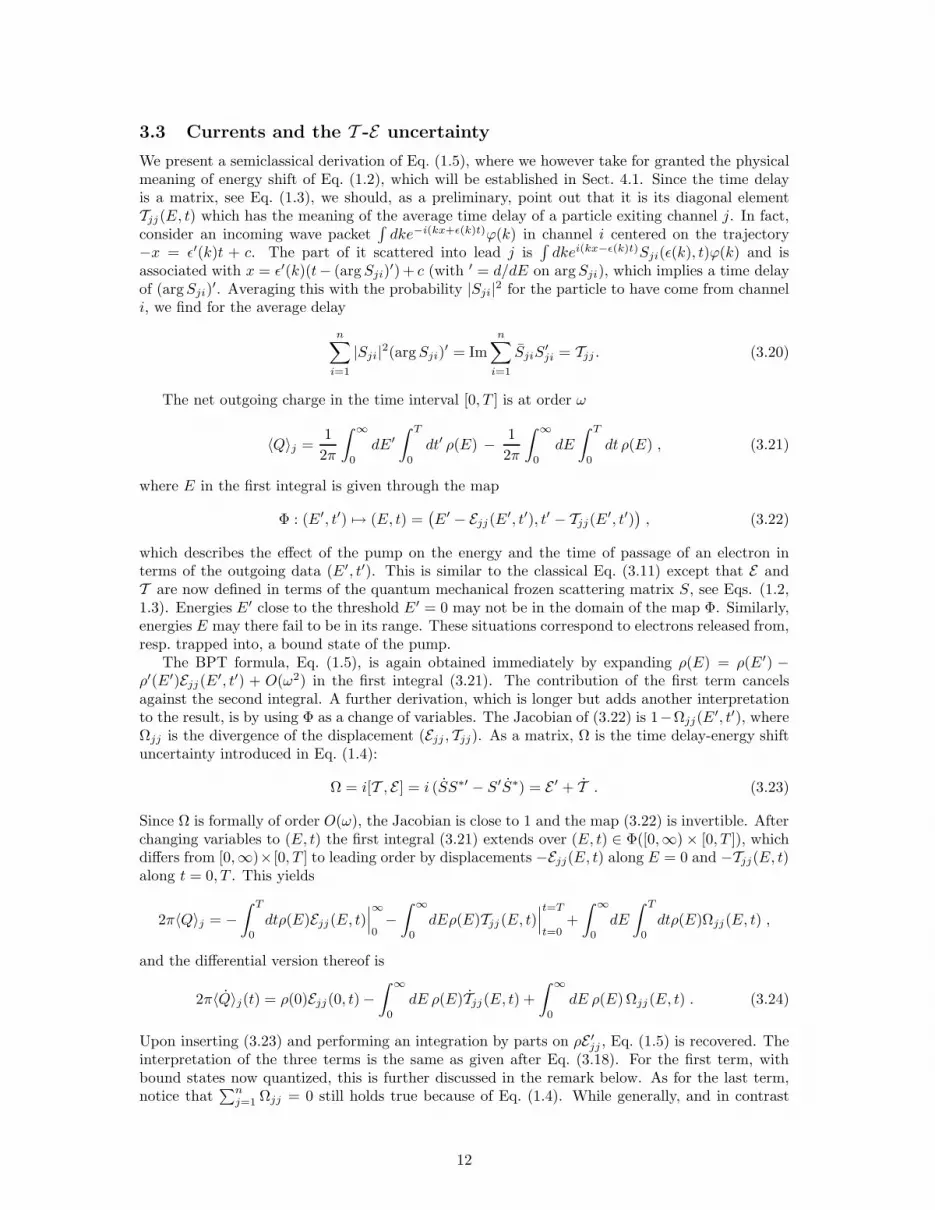
3.3 Currents and the T -E uncertainty

We present a semiclassical derivation of Eq. (1.5), where we however take for granted the physicalmeaning of energy shift of Eq. (1.2), which will be established in Sect. 4.1. Since the time delayis a matrix, see Eq. (1.3), we should, as a preliminary, point out that it is its diagonal elementTjj(E, t) which has the meaning of the average time delay of a particle exiting channel j. In fact,consider an incoming wave packet

∫

dke−i(kx+ǫ(k)t)ϕ(k) in channel i centered on the trajectory−x = ǫ′(k)t + c. The part of it scattered into lead j is

∫

dkei(kx−ǫ(k)t)Sji(ǫ(k), t)ϕ(k) and isassociated with x = ǫ′(k)(t− (argSji)

′) + c (with ′ = d/dE on argSji), which implies a time delayof (argSji)

′. Averaging this with the probability |Sji|2 for the particle to have come from channeli, we find for the average delay

n∑

i=1

|Sji|2(argSji)′ = Im

n∑

i=1

SjiS′ji = Tjj . (3.20)

The net outgoing charge in the time interval [0, T ] is at order ω

〈Q〉j =1

2π

∫ ∞

0

dE′∫ T

0

dt′ ρ(E) − 1

2π

∫ ∞

0

dE

∫ T

0

dt ρ(E) , (3.21)

where E in the first integral is given through the map

Φ : (E′, t′) 7→ (E, t) =(

E′ − Ejj(E′, t′), t′ − Tjj(E

′, t′))

, (3.22)

which describes the effect of the pump on the energy and the time of passage of an electron interms of the outgoing data (E′, t′). This is similar to the classical Eq. (3.11) except that E andT are now defined in terms of the quantum mechanical frozen scattering matrix S, see Eqs. (1.2,1.3). Energies E′ close to the threshold E′ = 0 may not be in the domain of the map Φ. Similarly,energies E may there fail to be in its range. These situations correspond to electrons released from,resp. trapped into, a bound state of the pump.

The BPT formula, Eq. (1.5), is again obtained immediately by expanding ρ(E) = ρ(E′) −ρ′(E′)Ejj(E

′, t′) + O(ω2) in the first integral (3.21). The contribution of the first term cancelsagainst the second integral. A further derivation, which is longer but adds another interpretationto the result, is by using Φ as a change of variables. The Jacobian of (3.22) is 1−Ωjj(E

′, t′), whereΩjj is the divergence of the displacement (Ejj , Tjj). As a matrix, Ω is the time delay-energy shiftuncertainty introduced in Eq. (1.4):

Ω = i[T , E ] = i (SS∗′ − S′S∗) = E ′ + T . (3.23)

Since Ω is formally of order O(ω), the Jacobian is close to 1 and the map (3.22) is invertible. Afterchanging variables to (E, t) the first integral (3.21) extends over (E, t) ∈ Φ([0,∞) × [0, T ]), whichdiffers from [0,∞)× [0, T ] to leading order by displacements −Ejj(E, t) along E = 0 and −Tjj(E, t)along t = 0, T . This yields

2π〈Q〉j = −∫ T

0

dtρ(E)Ejj(E, t)∣

∣

∣

∞

0−

∫ ∞

0

dEρ(E)Tjj(E, t)∣

∣

∣

t=T

t=0+

∫ ∞

0

dE

∫ T

0

dtρ(E)Ωjj(E, t) ,

and the differential version thereof is

2π〈Q〉j(t) = ρ(0)Ejj(0, t) −∫ ∞

0

dE ρ(E)Tjj(E, t) +

∫ ∞

0

dE ρ(E)Ωjj(E, t) . (3.24)

Upon inserting (3.23) and performing an integration by parts on ρE ′jj , Eq. (1.5) is recovered. The

interpretation of the three terms is the same as given after Eq. (3.18). For the first term, withbound states now quantized, this is further discussed in the remark below. As for the last term,notice that

∑nj=1 Ωjj = 0 still holds true because of Eq. (1.4). While generally, and in contrast

12

to the classical case, Ω may have full support in phase space, it remains true that it vanishes ifscattering is deterministic: If on some open subset of phase space

Sji(E, t) = 0 for i 6= π(j), (3.25)

where π is some fixed permutation of the channels, then S∗ is in the same manner related to π−1,and E , T to the identity permutation, i.e., they are both diagonal matrices. Hence Ω = 0 by (1.4).

Remark 3.1 The first term on the r.h.s. of (3.24) typically consists of delta functions located attimes t where the pump has a semi-bound state at a band edge, i.e., a state which can be turned eitherinto a bound state or a scattering state by an arbitrarily small change of the pump configuration.We illustrate this for ǫ(k) = k2, and first claim: either S(0, t) ≡ limE↓0 S(E, t) = −1, or the(static) pump at time t admits a semi-bound state. This is seen as follows: For each k ∈ C the 2nplane waves

ei cos kx , eisinkx

k, (3.26)

(eini=1 being the standard basis of Cn), form a basis of solutions with energy k2 in the n discon-

nected leads. Upon connecting them to the scatterer an n-dimensional subspace of solutions is left,which depends analytically on k. Since the dependence of (3.26) is also analytic, solutions may bewritten as

ψk(x) =

n∑

i=1

αiei cos kx+ βieisin kx

k, (3.27)

with amplitudes α = (α1, . . . , αn), β = (β1, . . . , βn) satisfying a set of linear equations

A(k)α+B(k)β = 0 (3.28)

with analytic n × n coefficient matrices A, B. As (3.28) defines an n-dimensional subspace, wehave rank (A,B) = n. For k = 0 (3.26) reduce to ei, eix. By a semi-bound state we mean moreprecisely a bounded solution ψ0(x), i.e., one with β = 0 in (3.27). Its existence is tantamountto detA(0) = 0. If detA(0) 6= 0, (3.28) can be solved for α at small k: α = −A(k)−1B(k)β,with arbitrary β ∈ Cn. For k > 0, the scattering matrix maps the incoming part of (3.27) to itsoutgoing part, ikα+ β = S(k2)(ikα− β). Thus

S(k2) = (−ikA(k)−1B(k) + 1)(−ikA(k)−1B(k) − 1)−1 → −1 , (k → 0) . (3.29)

This proves the claim, and in particular that E(0, t) = 0 except at times t when the scatterer has asemi-bound state. To discuss its behavior there, say this happens at t = 0, we assume genericallythat C(k, t) = B(k, t)−1A(k, t) (= C(k, t)∗) has a simple eigenvalue γ(k, t) with a first order zero atk = t = 0. Let P be its eigenprojection at crossing and let σ = sgn γ(0, 0) be the crossing direction.Then, we claim,

limE↓0

E(E, t) dt = −2πσPδ(t) dt , (3.30)

so that in the process, by (2.1), the charge

− limE↓0

1

2π

∫ ǫ

−ǫ

tr E(E, t) dt = σ (3.31)

is captured at arbitrarily small energy. Since the l.h.s. also equals limE↓0 arg detS(E, t)|ǫ−ǫ, (3.31)states that the phase of S(0, t) changes by 2π upon capture of a bound state, which is a dynamicalversion of Levinson’s theorem. The proof of (3.30) rests on the approximation of (3.29)

S(k2, t) =ikP − (γ′(0, 0)k + γ(0, 0)t)

ikP + (γ′(0, 0)k + γ(0, 0)t), (3.32)

valid near k = t = 0.

13

4 Time dependent scattering and Weyl calculus

4.1 The energy shift

In this section we describe the notion of energy shift in the context of time dependent scatteringtheory and derive an operator identity relating the outgoing density ρout to the incoming densityand the energy shift.

Energy is conserved in time independent scattering but not in time dependent scattering. Thisleads to an important differences between the S-matrix in the time independent and the timedependent case: In the time dependent case the S-matrix acquires a dependence on time shifts.Since this observation is not particular to pumps, it is simpler to describe it in general terms.

Using the conventional notation of scattering theory, let H0 be our reference, time independent,Hamiltonian (often called the free Hamiltonian) and H = H0 + V the scattering Hamiltonian. Vmay be time dependent. We assume that H and H0 admit a good scattering theory. In the timeindependent case, conservation of energy is expressed as the statement that the scattering matrixS commutes with H0 (not H !). Hence, for the frozen S-matrix

Sfe−iH0t = e−iH0tSf . (4.1)

This may be interpreted as the statement that the state ψ, and the time shifted state e−iH0tψboth see the same scatterer. Therefore it makes no difference if the time shift takes place beforeor after the scattering.

This is, of course, not true in the time-dependent case. The states ψ and its time shift e−iH0tψdo not see the same scatterer. Consequently, the exact (dynamical) scattering matrix, Sd, for atime dependent problem, acquires a time dependence:

Sd(t)e−iH0t = e−iH0tSd. (4.2)

Now Sd(t) will, in general, not coincide with Sd except, of course, at t = 0 since energy is notanymore conserved. In the time dependent case one does not have one scattering matrix, but rathera family of them, Sd(t). Since they are all related by conjugation, any one of them is equivalentto any other. To pick one, is to pick a reference point on the time axis. We shall use the notationSd(0) = Sd.

If Sd is unitary8, which we henceforth assume, then Ed = iSdS∗d is Hermitian. We call it the

“energy shift” for the following reason: Sd satisfies the equation of motion

iSd(t) = [H0, Sd(t)]. (4.3)

Using the (assumed) unitarity of Sd, this can be reorganized as

Sd(t)H0S∗d(t) = H0 − Ed(t). (4.4)

Conjugation by the scattering matrix takes outgoing observables to incoming observables. Eq. (4.4)justifies identifying Ed with the operator of energy shift.

Remark 4.1 If we let Qj denote the projection on the states in the j-th channel, then Qj =SdQjS

∗d projects on the out states fed by the j-th channel. The energy shift generates the evolution

of Qj:

i˙Qj = [Ed, Qj] (4.5)

We are now ready to derive Eq. (1.1) which is an operator identity for ρout. This is ourstarting point in analyzing adiabatic transport. By the functional calculus we can extend Eq. (4.4),evaluated at t = 0, to (measurable) functions of H0, namely

ρout = Sdρ(H0)S∗d = ρ

(

H0 − Ed

)

. (4.6)

So far, no approximation has been made. The identity does not assume an adiabatic time depen-dence.

8Sd is unitary as a map between the spaces of in and out states which may differ because states may get trappedor released from the pump.

14

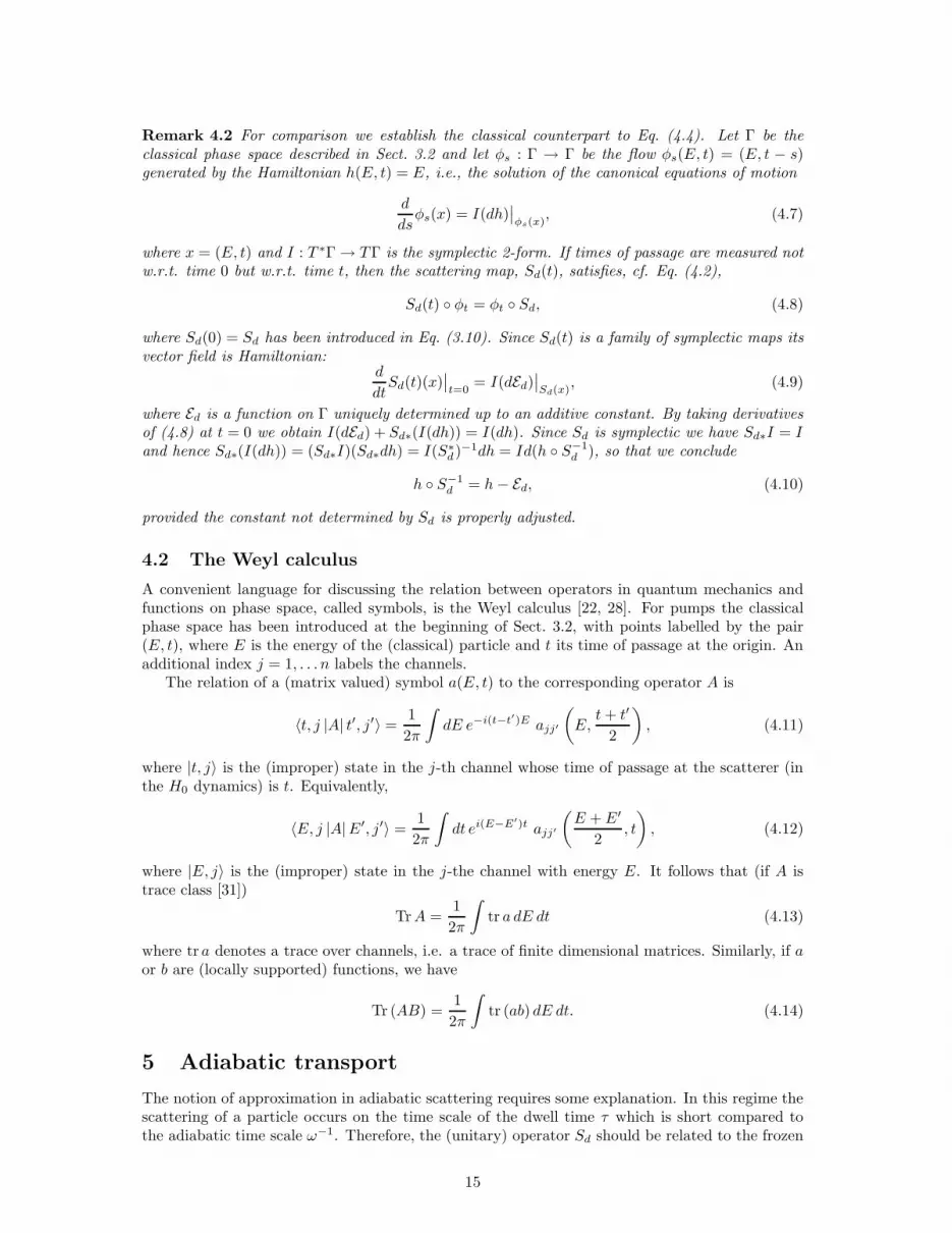
Remark 4.2 For comparison we establish the classical counterpart to Eq. (4.4). Let Γ be theclassical phase space described in Sect. 3.2 and let φs : Γ → Γ be the flow φs(E, t) = (E, t − s)generated by the Hamiltonian h(E, t) = E, i.e., the solution of the canonical equations of motion

d

dsφs(x) = I(dh)

∣

∣

φs(x), (4.7)

where x = (E, t) and I : T ∗Γ → TΓ is the symplectic 2-form. If times of passage are measured notw.r.t. time 0 but w.r.t. time t, then the scattering map, Sd(t), satisfies, cf. Eq. (4.2),

Sd(t) φt = φt Sd, (4.8)

where Sd(0) = Sd has been introduced in Eq. (3.10). Since Sd(t) is a family of symplectic maps itsvector field is Hamiltonian:

d

dtSd(t)(x)

∣

∣

t=0= I(dEd)

∣

∣

Sd(x), (4.9)

where Ed is a function on Γ uniquely determined up to an additive constant. By taking derivativesof (4.8) at t = 0 we obtain I(dEd) + Sd∗(I(dh)) = I(dh). Since Sd is symplectic we have Sd∗I = Iand hence Sd∗(I(dh)) = (Sd∗I)(Sd∗dh) = I(S∗

d)−1dh = Id(h S−1d ), so that we conclude

h S−1d = h− Ed, (4.10)

provided the constant not determined by Sd is properly adjusted.

4.2 The Weyl calculus

A convenient language for discussing the relation between operators in quantum mechanics andfunctions on phase space, called symbols, is the Weyl calculus [22, 28]. For pumps the classicalphase space has been introduced at the beginning of Sect. 3.2, with points labelled by the pair(E, t), where E is the energy of the (classical) particle and t its time of passage at the origin. Anadditional index j = 1, . . . n labels the channels.

The relation of a (matrix valued) symbol a(E, t) to the corresponding operator A is

〈t, j |A| t′, j′〉 =1

2π

∫

dE e−i(t−t′)E ajj′

(

E,t+ t′

2

)

, (4.11)

where |t, j〉 is the (improper) state in the j-th channel whose time of passage at the scatterer (inthe H0 dynamics) is t. Equivalently,

〈E, j |A|E′, j′〉 =1

2π

∫

dt ei(E−E′)t ajj′

(

E + E′

2, t

)

, (4.12)

where |E, j〉 is the (improper) state in the j-the channel with energy E. It follows that (if A istrace class [31])

TrA =1

2π

∫

tr a dE dt (4.13)

where tr a denotes a trace over channels, i.e. a trace of finite dimensional matrices. Similarly, if aor b are (locally supported) functions, we have

Tr (AB) =1

2π

∫

tr (ab) dE dt. (4.14)

5 Adiabatic transport

The notion of approximation in adiabatic scattering requires some explanation. In this regime thescattering of a particle occurs on the time scale of the dwell time τ which is short compared tothe adiabatic time scale ω−1. Therefore, the (unitary) operator Sd should be related to the frozen

15

scattering matrices S(E, t). While the uncertainty relation forbids specifying both coordinates Eand t of a particle, the variables on which S(E, t) actually depends are E and ωt. This givesadiabatic scattering a semiclassical flavor where ω plays the role of ~. Its theory can be phrasedin terms of the Weyl calculus [22, 28] with symbols which are power9 series in ω. In particular, aswe shall explain, S(E, t) may be interpreted as the principal symbol of Sd. The chain of argumentin making the identification goes through the frozen S-matrix, Sf (t), where the time of freezing, t,is picked by the incoming state.

5.1 Adiabatic scattering

We shall show the following correspondence between operators and symbols which, in our case, aren× n matrix functions of E and t:

Sd(t0) ⇐⇒ S(E, t+ t0) +O(ω) (5.1)

Ed ⇐⇒ E(E, t) +O(ω2) (5.2)

ρout ⇐⇒ ρ(E) − ρ′(E)(

E(E, t) +O(ω2))

+1

2ρ′′(E)E2(E, t) +O(ω3) (5.3)

Since the Fermi function at T = 0 is a step function, ρ′ is a delta function and consequently, thenotion of smallness in the expansion in Eq. (5.3) is in the sense of distributions10.

To see the first relation, let |t, j〉 denote the state that traverses the scatterer at time t andSf (s) denote the frozen S-matrix associated with the Hamiltonian in effect at time s. Then

〈t, j |Sd| t′, j′〉 =

⟨

t, j

∣

∣

∣

∣

Sf

(

t+ t′

2

)∣

∣

∣

∣

t′, j′⟩

+O(ω) (5.4)

The matrix elements on both sides are significant provided t− t′ is small, within the order of thedwell time, or the Wigner time delay. Using

|t, j〉 = (2π)−1/2

∫

dE eiEt |E, j〉 (5.5)

one finds

〈t, j |Sf (s)| t′, j′〉 =1

2π

∫

dE e−i(t−t′)E S(E, s), s =t+ t′

2, (5.6)

and we have used the fact that Sf is energy conserving. This establishes Eq. (5.1) for t0 = 0 bycomparison with Eq. (4.11). In the language of pseudo-differential operators S(E, t) is the principalsymbol of Sd. More generally, S(E, t + t0) is the principal symbol of Sd(t0). The “quantization”of S(E, t) then satisfies Eq. (4.2), as it must.

Eqs. (5.2, 5.3) now follow from the rules of pseudo-differential calculus [28], and the operatoridentity for the outgoing states Eq. (1.1).

5.2 Currents

A rigorous derivation of BPT is presented in [9, 29]. Here, instead, we shall be content with aformal, but relatively straightforward derivation using Weyl calculus.

Let Qin/outj (x, t0) be the observable associated with counting the incoming/outgoing particles

in a box that lies to the right of a point x in the j-th channel at the point in time t0. The point xis chosen far from the scatterer, but not so far that the time delay relative to the pump is of orderω−1. Namely, vτ ≪ x≪ v/ω. The symbol of Qin/out is a matrix valued step function:

Qin/outj (x, t0) ⇐⇒ Pj θ

(

v(t0 − t) − x)

θ(∓(t0 − t)), (Pj)ik = δjkδij , v = ǫ′(p), (5.7)

and Pj is the projection matrix on the j-th channel. Indeed, the position of a particle withcoordinates (E, t) at time 0 will be −v(t− t0) at time t0, see Eq. (3.9). The particle will then be

9The dimensionless expansion parameter is ωτ .10In agreement with Eqs. (2.8, 2.13).

outgoing if t− t0 < 0. Notice that t = t0 falls outside of the support of the first Heaviside function.The associated incoming/outgoing current operators are

Qin/outj (x, t0) = i[H,Q

in/outj (x, t0)] = i[H0, Q

in/outj (x, t0)]. (5.8)

Here we used the fact that beyond x, deep inside the channel, H(t) coincides with H0. The symbolassociated with the current is most easily computed recalling that in Weyl calculus commutatorsare replaced by Poisson brackets. This reproduces the usual notion of a current

Qin/outj (x, t0) ⇐⇒ Pj E, θ

(

v(t− t0) − x)

= ∓Pj δ(

t− t0 − x/v)

θ(∓(t0 − t)), (5.9)

x is where the “ammeter” is localized. By the assumption that the ammeter is not too far it leadsto a slight modification of t0, the time when current is measured. We henceforth drop x. Now theexpectation value of the current is

〈Q〉j(x, t0) = Tr(

ρoutQoutj

)

+ Tr(

ρQinj

)

= Tr(

δρ Qoutj (x, t0)

)

, δρ = ρout − ρ. (5.10)

Using Eq. (4.14) to evaluate the trace we find

〈Q〉j(x, t0) = − 1

2π

∫

dE dt ρ′(E)Ejj(E, t)δ(t− t0) +O(ω2)

= − 1

2π

∫

dE ρ′(E)Ejj(E, t0) +O(ω2) (5.11)

reproducing Eq. (1.5).

5.3 Dissipation

To compute the dissipation we start as in the previous section. Let Din/outj denote the observable

associated with the incoming/outgoing excess energy in the j-th channel in a box to the right ofthe point x. The excess energy is, of course, energy measured relative to the Fermi energy:

Din/outj (x, t0) =

1

2Qin/out

j (x, t0), H0 − µ (5.12)

and Qin/outj is as in Eq. (5.7). The observable associated with dissipation current in the j-th

channel is the time derivative of the excess energy, i.e.,

Din/outj (x, t0) = E

in/outj (x, t0) − µQ

in/outj (x, t0) = i

[

H0, Din/outj (x, t0)

]

. (5.13)

The symbol corresponding to the dissipation current is then

Din/outj (x, t0) ⇐⇒ ∓Pj (E − µ) δ

(

t− t0 − x/v)

θ(∓(t0 − t)). (5.14)

The expectation value of the dissipation current is therefore

〈D〉j(x, t0) = Tr(

δρ Doutj (x, t0)

)

. (5.15)

We shall now show that for T .√

ω/τ the dissipation is quadratic in ω and is determined byEq. (1.6).

As in section 5.2 we shall evaluate the trace using Eq. (4.14). At low temperature ρ′ is con-centrated near the Fermi energy. We may then approximate the energy shift up to its linearvariation near µ. For the term proportional to ρ′ in the expansion Eq. (5.3) the contribution tothe dissipation is proportional to

− 1

2π

∫

dE ρ′(E)(

Ejj(µ, t0) + (E − µ)E ′jj(µ, t0) +O(ω2)

)

(E − µ)

= O(

βe−βµ)

+O(ωT 2) +O(ω2T ). (5.16)

17

The term proportional to ρ′′ in the expansion gives,

1

4π

∫

dE ρ′′(E)(E2)jj(E, t0)(E − µ) =1

4π(E2)jj(µ, t0) +O(ω2T ), (5.17)

which is the requisite result, Eq. (1.6).The result (1.6) is remarkable in that we obtain the dissipation to order ω2 by making two

approximations, each valid only to order ω. First we replace Ed with E , and then we evaluate Eat E = µ. Had we used this procedure to compute the quantities Ej and Qj separately, each ofthem would be off by nonzero O(ω2) terms (as can be seen in the snowplow and battery examples);nevertheless, the combination Ej − µQj is computed correctly to order ω2. The reason is that ineach quantum channel one has the following lower bound on the dissipation [7]:

Ej − µQj ≥ πQ2j . (5.18)

This bound is saturated by the outgoing population distribution that is filled up to energy µ andempty thereafter. The dissipation should therefore be quadratic in the deviation of the outgoingdistribution from this minimizer. Since the outgoing distribution is an O(ω) perturbation of theminimizer, knowing the distribution to order ω should give the dissipation to order ω2.

Remark 5.1 There would appear to be two problems with the argument above. In minimizing afunctional on a region with a boundary, one obtains a quadratic estimate for the functional aroundits minimizer if the minimum occurs at an interior point. If the minimum occurs at the boundary,then a variation away from the boundary can increase the function to first order. Furthermore,whether the minimum occurs at an interior point or on the boundary, quadratic estimates dependon the Hessian being a bounded operator. If the Hessian is unbounded, then an arbitrarily smallchange in the point can cause an arbitrarily large increase in the functional. In our case, theminimum occurs at a point that is on the boundary of the constraints 0 ≤ ρ(E) ≤ 1. There arelarge modes for the Hessian, involving adding electrons at arbitrarily high energies.

Fortunately, neither exception is relevant. In fact, the correction of the distribution, as givenby (5.3), consists of a local reshuffling of electrons around the Fermi energy and does not involvethe large modes of the Hessian. These variations should not be viewed as being either towards oraway from the boundary, since neither the expression (4.6) nor its opposite (replacing E with −E)violates the constraints.

5.4 Entropy and noise currents

Entropy and noise introduce a new element in that the transport equation, Eq. (1.7), depends onthe density through a non-linear function h(ρ). For the entropy and noise h(x) is given in Eq. (1.8).Using the fact that in either case h(0) = h(1) = 0, we shall show that for ω ≪ T ≪

√

ω/τ thecurrents are quadratic in ω and are given by

sj(t, µ, T ) =β

2π∆E2

j (µ, t))

∫ 1

0

dxh(x) , (5.19)

where ∆E2j has been defined in Eq. (1.10). For the entropy the integral gives 1/2 and for the

noise it gives 1/6. To complete the derivation of the noise and entropy currents, we now deriveEq. (5.19).

The condition ω ≪ T makes it possible to consider the outgoing state of the electrons with afixed time of passage, provided the time resolution is short compared to ω−1 but large w.r.t. T−1.The state ρout,j = PjρoutPj is then given, see (5.3), as

ρout,j(E) = ρ(E − Ejj(E, t)) +1

2ρ′′(E)

(

(E2)jj(E, t) − Ejj(E, t)2)

. (5.20)

The entropy/noise current (1.7) is

1

2π

∫

dE(

(h ρ)(E − Ejj(E, t)) − (h ρ)(E))

+1

4π

∫

dE (h′ ρ)(E)ρ′′(E)∆E2j (E, t). (5.21)

18

In these integrals, Ejj may be regarded as constant in E because of the condition T ≪√

ω/τ .The first integral then vanishes and in the second we may pull ∆E2

j (µ, t) out of the integral. Thisleaves us with the integral

∫

dE (h′ ρ)(E) ρ′′(E) = −β∫ 1

0

dρ h′(ρ) (1 − 2ρ) = 2β

∫ 1

0

dρ h(ρ), (5.22)

where, in the second step, we have used a property of the Fermi function, ρ′ = −β ρ(1 − ρ), andan integration by parts in the last step. This establishes the result.

We have nothing to say about the range T . ω. The noise at T = 0 can be calculated using aformalism of Lesovik and Levitov that we discuss in the appendix. This formula is nonlocal in time.It is instructive to examine what goes wrong with our approach at T = 0. In this limit ρ′ and ρ′′

are distributions and ρ a discontinuous function. Since it is not allowed to multiply distributionsby distributions, or even by discontinuous functions, equations such as Eq. (5.22) which are notlinear in ρ make no sense. This is a reflection of the fact that in the regime where T . ω entropyand noise currents have a memory that goes back in times of order β. In the regime we considerω ≪ T the memory is short compared with the time scale of the pump and instantaneous formulasmake sense. At the opposite regime, where T . ω, a local formula in time cannot be expected.

6 Examples

Quantum pumps may be viewed either as particle pumps or as wave pumps. The particle interpre-tation has a classical flavor where the driving mechanism is identified with forces on the particles.The wave interpretation stresses the role played by phases and suggests that interference phenom-ena play a role. This duality can be seen in the BPT formula in the two channel case of section2. On the one hand Eq. (2.5) makes it clear that the phases in the S-matrix, (α, φ, γ), play a rolein charge transport. In fact, changing the transmission and reflection probabilities while keepingthe phases fixed cannot drive a current. At the same time, the rate of change of two of the threephases, φ and α, also admit a classical interpretation as EMF and Galilean shift. The pedestrianderivation is a reflection of the fact that particle interpretation is more intuitive. Here we shallconsider two examples where dual reasoning is insightful.

6.1 The bicycle pump

In a bicycle pump the action of the valves is synchronized with the motion of the piston. Theanalogous quantum pump has synchronized gates as shown in Fig. 6. The particle interpretationof the pump is simple and intuitive. The wave (or BPT) point of view is more subtle. In particularas we shall see, in terms of the elementary processes described in section 2 the pump operates bychanging the phases γ and α: Galilean shifts arise from the synchronized action of the gates.

Let us choose a length scale so that kF = π and an energy scale so that µ = 1. In theseunits, choose the length of the pump, L, to be an integer L = n, pick the valves thin, δ ≪ 1,and impenetrable, i.e., of height M with Mδ ≫ 1. Consider the potential, shown in Fig. 6, thatdepends on two parameters, a and b, that vary on the boundary of the unit square [0, 1]× [0, 1]:

Va,b(x) =

0 if x < 0,,

aM if 0 ≤ x < δ,

10 b if δ ≤ x < L

(1 − a)M if L ≤ x < L+ δ

0 if x ≥ L+ δ.

(6.1)

Since the quantum box was designed to accommodate n particles, the pumps transfers n particlesin each cycle. Like in the bicycle pump, at all times, at least one of the valves is closed. This givethe particle point of view 11.

11For related results see e.g. [20].

19

aM

bML

(1-a)M

a

b

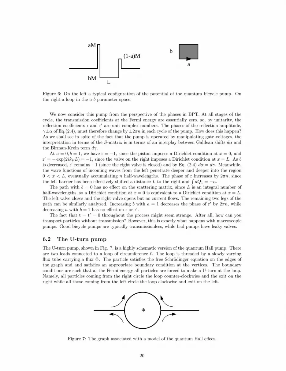
Figure 6: On the left a typical configuration of the potential of the quantum bicycle pump. Onthe right a loop in the a-b parameter space.

We now consider this pump from the perspective of the phases in BPT. At all stages of thecycle, the transmission coefficients at the Fermi energy are essentially zero, so, by unitarity, thereflection coefficients r and r′ are unit complex numbers. The phases of the reflection amplitude,γ±α of Eq.(2.4), must therefore change by ±2πn in each cycle of the pump. How does this happen?As we shall see in spite of the fact that the pump is operated by manipulating gate voltages, theinterpretation in terms of the S-matrix is in terms of an interplay between Galilean shifts dα andthe Birman-Krein term dγ.

At a = 0, b = 1, we have r = −1, since the piston imposes a Dirichlet condition at x = 0, andr′ = − exp(2ikFL) = −1, since the valve on the right imposes a Dirichlet condition at x = L. As bis decreased, r′ remains −1 (since the right valve is closed) and by Eq. (2.4) dα = dγ. Meanwhile,the wave functions of incoming waves from the left penetrate deeper and deeper into the region0 < x < L, eventually accumulating n half-wavelengths. The phase of r increases by 2πn, sincethe left barrier has been effectively shifted a distance L to the right and

∫

dQ1 = −n.The path with b = 0 has no effect on the scattering matrix, since L is an integral number of

half-wavelengths, so a Dirichlet condition at x = 0 is equivalent to a Dirichlet condition at x = L.The left valve closes and the right valve opens but no current flows. The remaining two legs of thepath can be similarly analyzed. Increasing b with a = 1 decreases the phase of r′ by 2πn, whiledecreasing a with b = 1 has no effect on r or r′.

The fact that t = t′ = 0 throughout the process might seem strange. After all, how can youtransport particles without transmission? However, this is exactly what happens with macroscopicpumps. Good bicycle pumps are typically transmissionless, while bad pumps have leaky valves.

6.2 The U-turn pump

The U-turn pump, shown in Fig. 7, is a highly schematic version of the quantum Hall pump. Thereare two leads connected to a loop of circumference ℓ. The loop is threaded by a slowly varyingflux tube carrying a flux Φ. The particle satisfies the free Schrodinger equation on the edges ofthe graph and and satisfies an appropriate boundary condition at the vertices. The boundaryconditions are such that at the Fermi energy all particles are forced to make a U-turn at the loop.Namely, all particles coming from the right circle the loop counter-clockwise and the exit on theright while all those coming from the left circle the loop clockwise and exit on the left.

Φ

Figure 7: The graph associated with a model of the quantum Hall effect.

20

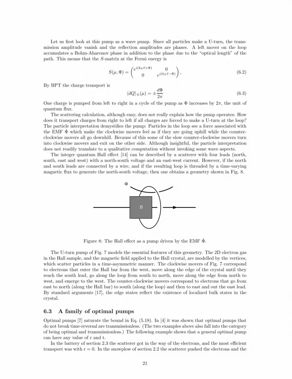
Let us first look at this pump as a wave pump. Since all particles make a U-turn, the trans-mission amplitude vanish and the reflection amplitudes are phases. A left mover on the loopaccumulates a Bohm-Aharonov phase in addition to the phase due to the “optical length” of thepath. This means that the S-matrix at the Fermi energy is

S(µ,Φ) =

(

ei(kF ℓ+Φ) 0

0 ei(kF ℓ−Φ)

)

, (6.2)

By BPT the charge transport is

〈dQ〉±(µ) = ±dΦ2π

(6.3)

One charge is pumped from left to right in a cycle of the pump as Φ increases by 2π, the unit ofquantum flux.

The scattering calculation, although easy, does not really explain how the pump operates: Howdoes it transport charges from right to left if all charges are forced to make a U-turn at the loop?The particle interpretation demystifies the pump: Particles in the loop see a force associated withthe EMF Φ which make the clockwise movers feel as if they are going uphill while the counter-clockwise movers all go downhill. Because of this some of the slow counter-clockwise movers turninto clockwise movers and exit on the other side. Although insightful, the particle interpretationdoes not readily translate to a qualitative computation without invoking some wave aspects.

The integer quantum Hall effect [14] can be described by a scatterer with four leads (north,south, east and west) with a north-south voltage and an east-west current. However, if the northand south leads are connected by a wire, and if the resulting loop is threaded by a time-varyingmagnetic flux to generate the north-south voltage, then one obtains a geometry shown in Fig. 8.

B

Φ

Figure 8: The Hall effect as a pump driven by the EMF Φ.

The U-turn pump of Fig. 7 models the essential features of this geometry. The 2D electron gasin the Hall sample, and the magnetic field applied to the Hall crystal, are modelled by the vertices,which scatter particles in a time-asymmetric manner. The clockwise movers of Fig. 7 correspondto electrons that enter the Hall bar from the west, move along the edge of the crystal until theyreach the south lead, go along the loop from south to north, move along the edge from north towest, and emerge to the west. The counter-clockwise movers correspond to electrons that go fromeast to north (along the Hall bar) to south (along the loop) and then to east and out the east lead.By standard arguments [17], the edge states reflect the existence of localized bulk states in thecrystal.

6.3 A family of optimal pumps

Optimal pumps [7] saturate the bound in Eq. (5.18). In [4] it was shown that optimal pumps thatdo not break time-reversal are transmissionless. (The two examples above also fall into the categoryof being optimal and transmissionless.) The following example shows that a general optimal pumpcan have any value of r and t.

In the battery of section 2.3 the scatterer got in the way of the electrons, and the most efficienttransport was with r = 0. In the snowplow of section 2.2 the scatterer pushed the electrons and the

21

most efficient transport was with |r| = 1. In the following example of optimal pump we combine avoltage with a moving scatterer, such that the scatterer is moving along with the electrons, neitherpushing nor getting in the way. In this case, the scatterer doesn’t actually do anything, and weget efficient transport, regardless of the initial values of (r, t, r′, t′).

Write the scattering matrix of a system where α = 2µξ and φ evolve as

S(µ) =

(

re−2iµξ t′e−iφ

teiφ r′e2iµξ

)

, (6.4)

Synchronizing the velocity ξ with the voltage φ according to

2µξ = φ (6.5)

makes S = iφσ3S. The energy shift is then a diagonal matrix

E = iSS∗ = −φ σ3 (6.6)

which implies that the pump is optimal.

6.4 The phase space of a snowplow

We give a description of a classical snowplow moving on the real axis at speed v0 during thetime interval [−T, T ], but at rest before and after that. It is described by the (total) phase spaceR2 ∋ (x, p) with Hamiltonian function h = p2/2 + V (t), where V (t) is a barrier of fixed heightV > v2

0/2 and zero width located at

x(t) =

−v0T, (t ≤ −T ),

v0t, (−T < t < T ),

v0T, (t ≥ −T ).

(6.7)

We use the notation of Sect. 3.2 and denote by 1 the left channel (x < 0) and by 2 the right one(x > 0). Let Γ+

ij ⊂ Γj ⊂ Γ+ be the outgoing labeled trajectories originating from channel i and

eventually ending in channel j. The same meaning has Γ−ij ⊂ Γi ⊂ Γ−, except that the trajectories

are incoming labeled.If a particle crosses the above scatterer of zero width, then its trajectory is free at all times.

HenceΓ−

12 = Γ+12, Γ−

21 = Γ+21. (6.8)

It suffices to compute these subsets only. The remaining ones are then given by complementarity:

Γ−i1 ∪ Γ−

i2 = Γi, Γ+1j ∪ Γ+

2j = Γj , (6.9)

with disjoint unions.

• Γ−12 = Γ+

12. Depending on their time of passage t, trajectories of this type will (see Fig. 9)require an energy E = v2/2 > Ec ≡ v2

c/2, with critical energy Ec given as

Ec = V if |t| > T − v0vT = T − v0√

2ET ;

resp. by vc − v0 =√

2V , i.e.,

Ec =1

2(√

2V + v0)2 if |t| ≤ T − v0√

2ET.

This portion of phase space is drawn dark shaded in the upper part of Fig. 10.

22

T

t−T

T−

v0vT

x

t

−T

+v0

vT

v

v0

Figure 9: The thick line represents the position x(t) of the snowplow. The other lines are freetrajectories of common energy E indicated by the slope v =

√2E > 0. Their times of passage t

are read off at the intercepts with the abscissa.

• Γ−21 = Γ+

21. In this case the slope of free trajectories is v = −√

2E < 0. As a result thecritical energy Ec is

Ec = V if |t| > T +v0√2E

T,

Ec =1

2(√

2V − v0)2 if |t| ≤ T +

v0√2E

T.

This portion of phase space is drawn dark shaded in the lower part of Fig. 10.

6.5 Classical scattering from a battery

This example shows that, in the classical case, static scattering data cannot determine the en-ergy shift. Consider the classical version of the battery, see Sect. 2.3, with Hamiltonian functionh(x, p) = (p−A)2/2 and gauge A(x, t) = tφ′(x) of compact support. Clearly, this describes parti-cles which get accelerated as they cross the pump, whence there is an energy shift. More formally,the quantity f(x, p) = (p − A)2/2 + φ is a constant of motion, as it is verified from Newton’sequation (d/dt)(p − A) = −A = −φ′. In the leads, f = p2/2 + φ, which implies that the energyE = p2/2, as defined there, gets shifted by E = −φ|∞−∞ if a particle crosses the battery from leftto right. On the other hand, for each static scatterer, p − A is a constant of motion, whence thestatic scattering maps all equal the identity map! The quantum mechanical phase information,which was present in the static S-matrix and determined the energy shift, is of course unavailablehere.

7 Geometry and topology

When a pump goes through a cycle, so does the scattering matrix S(E, t). The rows of matrixdefine unit vectors in Cn and the charge transport in the j-th channel can be interpreted in termsof geometric properties of these vectors.

As we shall explain in section 7.2, the charge transport is naturally identified with the globalangle accumulated by a row of the S-matrix during a cycle. It need not be an integer multiple of2π. Computing this angle is formally the same as computing Berry’s phase [10]. That the globalphase has direct physical significance is related to the fact that a quantum pump is a wave pump.

Interestingly, the charge transport in a closed cycle can also be computed by forgetting al-together about the (global) phase provided one has knowledge about what happens on a surfacespanning this cycle. This reflects a basic geometric relation between the failure of parallel transportand the curvature.

23

E

t

12(√

2V + v0)2

V

12(√

2V − v0)2

−T T

Γ−11 = Γ+

22

E

t

12(√

2V + v0)2

V

12(√

2V − v0)2

−T T

Γ−21 = Γ+

21

Γ−22 = Γ+

11

Γ−12 = Γ+

12

Figure 10: Portions of phase space corresponding to transmitted (dark shaded) and reflected (lightshaded) trajectories with labels +/− corresponding to outgoing/incoming data. The curves on theright halves correspond to t = T ± v0√

2ET .

7.1 Charge transport and Berry’s phase

Let

|ψj〉 =

Sj1

Sj2

...Sjn

∈ Cn (7.1)

be the transpose of the j-th row of the frozen S matrix, evaluated at the Fermi energy. Yet anotherrewriting of the BPT formula at zero temperature is as

2π〈dQ〉j = i〈ψj |dψj〉. (7.2)

The expression on the right hand side is familiar from the context of adiabatic connections andBerry’s phase [10]. To simplify notation we shall fix a row, say the first, and drop the index j.

There are important conceptual differences between the Berry’s phase associated to a quantumstate |ψ〉 and the phases that arise in the study of a row of the S-matrix |ψ〉. In the usual Berry’sphase setting one starts with a circle of Hamiltonians to which one associates a (unique) circle ofprojections |ψ〉〈ψ|, say on the ground state. To represent these projections in terms of a circle ofeigenvectors |ψ〉 one needs to choose a reference phase arbitrarily for each point on the circle. Thephysical adiabatic evolution picks its own phase relative to the reference phase. Berry’s phase thenmeasures the phase accumulated in a cycle12. In particular, it does not make sense to talk aboutthe phase accumulated on a path that is not closed.

12By choosing the energy of the state to be zero one can always get rid of the dynamic phase.

24

In contrast, a cycle of the pump is a circle of vectors |ψ〉 of the scattering matrix (not a cycleof projections). No choice of a phase needs to be made—the phases are all fixed by solving thescattering problem. In particular, the vector |ψ〉 always returns to itself after a complete cycle ofthe pump. Moreover, unlike the usual Berry’s phase, Eq. (7.2) makes perfectly good physical andmathematical sense also for an open path and not just for a closed cycle.

What, then, does the Berry’s phase measure in the present context? This is addressed in thenext section.

7.2 Global angle

As we now explain the charge transport in a quantum pump has a geometric interpretation interms of the global angle of |ψ〉.

The notion of global angle is obvious in the case that the circle of vectors are all parallel, i.e.,

|ψ〉 = eiγ |ψ0〉 (7.3)

with |ψ0〉 fixed. The global angle is γ and is related to the charge 2π〈dQ〉 = −dγ.Now, how do we compare global angles when vectors are not parallel? This is a classical

problem in geometry whose answer relies on the notion of parallel transport. Namely, one needs arule for taking one vector to another without changing its global phase. A natural way to do so isto impose that there be no motion in the “direction” |ψ〉〈ψ|. Explicitly, we say that |ψ〉 is paralleltransported if

|ψ〉〈ψ|dψ〉 = 0 (7.4)

We can now compare the global phase for any two vectors connected by a path. The path maybe either open or closed, and the global angle makes sense in either case. The right hand side ofEq. (7.2) is (minus) the change in the global angle and the left hand side identifies it with thetransported charge. This identifies charge transport with a global angle.

The global angle need not change by a multiple of 2π in a cycle of the pump—except in thespecial case that |ψ〉 = eiγ |ψ0〉 with |ψ0〉 fixed. The failure of parallel transport for closed pathsis interpreted in geometry as curvature.

7.3 Curvature

In the previous section we identified charge transport with the global angle of |ψj〉. Remarkably,one can compute the charge transport in a closed cycle while forgetting altogether about the globalphase and relying only on the projection |ψj〉 〈ψj |. For a closed cycle one can relate the line integralon the boundary of a disk ∂D to a surface integral on the disk D via Stokes

2π〈Q〉j = i

∫

∂D

〈ψj | dψj〉 = i

∫

D

〈dψj | dψj〉 (7.5)

In the context of pumps the identity is known as Brouwer’s formula [11].

Remark 7.1 For other ways to rewrite Eq. (7.5), use the identities

i 〈dψj | dψj〉 = −i(dS ∧ dS∗)jj = −iTr Pj(dPj ∧ dPj)Pj , (7.6)

where Pj = S∗PjS is the projection onto the state feeding channel j. The r.h.s. is the trace of the

curvature of the connection Pjd (see e.g. [5], Sect. 9.5).

We shall now describe a different interpretation of Brouwer’s formula that focuses on the Wignertime delay and the energy shift. We consider the charge transport in a cycle, so t is an angle. ByEq. (3.24), and assuming no semi-bound states, so E(0, t) = 0, the charge transport in a cycle is

2π〈Q〉j =

∫

C

dE ∧ dtΩjj (7.7)

25

where C is the cylinder [0, µ] × S. Now

Ωjj dE ∧ dt = dEjj ∧ dt+ dE ∧ dTjj = −i (dS ∧ dS∗)jj . (7.8)

The difference between this formula and Eq. (7.5) is the domain of integration: A disc in Brouwer’sformula, and a cylinder here. However, since E(0, t) = 0 the bottom of the cylinder may be pinchedto a point and the cylinder turns to a disk. The r.h.s. is the trace of the curvature of the connectionPjd (see e.g. [5], Sect. 9.5) or of its connection 1-form i[(dS)S∗]jj = Ejjdt − TjjdE. Similarequations are found in the context of the quantum Hall effect [32], see e.g. [5] Sect. 11.3), but,unlike there,

∫ µ

E−

∮

dE∧dtΩ(E, t)jj is not a Chern number as a rule, since the integration manifold

has a boundary.

7.4 The two channel case

The two channel case is particularly simple. |ψ〉 =

(

rt′

)

lives in S3. The projection associated to

|ψ〉 can be identified with a point on S2 according to

|ψ〉 〈ψ| =1 + n · ~σ

2(7.9)

where n is a unit vector in R3 and ~σ is the triplet of Pauli matrices. Eq. (7.5) then says that thecharge transport is half the spherical angle.

The claim that one can compute the charge transport in a closed cycle while forfeiting allknowledge of the global phase means, in the 2-channel case, that all that matters is z = r/t′. zlives in CP1 = C ∪ ∞ and is related to n above via the usual stereographic projection

|ψ〉 → (2Re(rt′), 2Im(rt′), |r|2 − |t′|2) =

(

2Re(z)

1 + |z|2 ,2Im(z)

1 + |z|2 ,|z|2 − 1

1 + |z|2)

, (7.10)

The curvaturei(drdr + dt′dt′) = i(1 + |z|2)−2dzdz, (7.11)

can be written entirely in terms of z. The current pumped by a small loop in parameter space cantherefore be computed by a calculation on S2.

For large loops, however, things are more subtle. If a path in parameter space maps to theequator, is the bounding region the northern hemisphere (area +2π) or the southern hemisphere(signed area −2π)? Because of this ambiguity, the path in S2 only determines the fractional partof the expected charge transported, not the integral part. In particular, if the path on the unitsphere is trivial—the ratio z = r/t′ is constant—then the fractional part is zero and the chargetransported is an integer. The bicycle pump, where t′ is identically zero, is an example of thisquantized transport.

How, then, can one determine also the integral part without a knowledge of the global phase?Consider a region in parameter space bounded by our path. The integral part is how many timesit wraps around S2 (i.e., the degree of the map). For the bicycle pump, this is counting how manypoints on the unit square [0, 1] × [0, 1] correspond to a particular value of z, say z = 0. In fact,since we know, be elementary arguments, that the charge transport in each cycle is n, there mustbe (at least) n points in the interior of the square where the potential is reflectionless at the Fermienergy.

7.5 Chern and winding numbers

Part of the motivation for pumps is as standards of charge transport, whence quantization is anissue. In this section we want to explain why Chern numbers in quantum pumps must vanish.Instead, in some cases, winding numbers play a role.

26

The Hopf fibration gives the unit sphere S2n−1 ⊂ Cn the structure of a U(1) principal bundleover CPn−1 via the map

π : S2n−1 −→ CPn−1 (7.12)

|ψ〉 −→ |ψ〉〈ψ|, (7.13)

where we realize CPn−1 as the set of all rank-1 projections in Cn.Chern numbers in transport theory [35] typically arise as follows. The physical parameter space

is a closed surface, M, say a sphere or a torus. The Hamiltonian, acting on the vector space Cn,is then a function on M, and any one of its simple eigenvalues map M to CPn−1. The pullback ofthe Hopf fibration is then a U(1) bundle over parameter space, with local geometry and possiblynontrivial topology. The integrated curvature is a Chern number, and may be nonzero.

In adiabatic pumps, however, the frozen S matrix defines a map from M directly to S2n−1, andindirectly to CPn−1. This gives a trivialization of the bundle, and shows that all Chern numbersare zero. Besides, as seen from Eq. (7.5), charge transport is the integral of the Chern characteri 〈dψj | dψj〉 over a surface D with boundary, and thus not given by a Chern number.

More appropriate is the point of view on pumps taken in the previous section, or its general-ization to n leads. If a pump operation is of the form (7.3), then

∮

〈dQ〉 is the winding number

of eiγ [3, 7]. Alternatively, the curvature Eq. (7.6) can be computed in terms of Pj = π(|ψ〉), cf.Eq. (7.11), and the integral (7.5) thus performed over π(D). The condition (7.3) means ∂π(D) = ∅,which again shows that

∮

〈dQ〉 is an integer.An example where this quantization occurs is the U-turn pump, section 6.2: The charge trans-

port in a cycle is the winding number of the map from the circle of fluxes to the circle of complexnumbers of modulus one. A small change of the parameters underlying Fig. 8 will only modifykF ℓ in the effective description by Eq. (6.2) and thus preserve quantization. On the other hand,if the U-turn pump is viewed as an example of a Schrodinger operator on a graph, then a genericperturbation in this class will destroy quantization.

7.6 Geometry of dissipation and noise

Eq. (1.6) and Eq. (1.9) that describe dissipation and entropy (and hence also noise) currents havea simple geometric interpretation in terms of the fiber bundle S2n−1 → CPn−1. The j-th row ofE describes the velocity of |ψ〉 in S2n−1. Of this, Ejj is the projection of this velocity onto the

fiber, and Ejk, with k 6= j, give the projection of this velocity onto CPn−1. The current 〈Qj〉,and the minimal dissipation |Ejj |2/4π, are both functions of motion in the fiber, while the excessdissipation

〈Ej〉 − µ〈Qj〉 − π〈Qj〉2 =1

4π

∑

k 6=j

|Ejk|2 (7.14)

is the “energy” (that is, squared velocity) associated with motion in the base. In particular, apump operation is of the form (7.3) if and only if the bound Eq. (5.18) is saturated, or equivalentlyif the noise at T > 0 or at T = 0, see Eqs. (1.9, A.19), vanishes. Such pumps may be called optimal[7] w.r.t. the j-th channel.

In an interesting piece of work Mirlin and Makhlin [23], relate the problem of finding a cyclewith minimal noise production at T = 0 to the problem of finding a minimal surfaces supportedby a given loop. This result is outside the scope of transport properties which are local in time, asit deals with T = 0 and the noise.

Acknowledgment JEA thanks I. Klich for many enlightening discussions on the Lesovik-Levitov formula. We thank M. Buttiker, J. Frohlich, M. Hager, B. Pedrini, K. Schnee, W. Zwergerfor discussions. This work is supported by the Technion fund for promotion of research and by theEU grant HPRN-CT-2002-00277.

27

A Comparison with the theory of full counting statistics

The formulas for the entropy and noise currents, Eq. (1.9), are singular in the limit T → 0. Thisappears to be in conflict with the Lesovik-Levitov’s formula (LL) which gives finite noise at T = 0(see below). We shall verify here that, in fact, for T & ω, LL is consistent with our results. Weshall start by recalling LL.

A.1 The Lesovik-Levitov formula

Here we shall describe a version of the Lesovik-Levitov formalism [19] where LL is an identityrather than an (adiabatic) approximation.

Assume that in the distant past and distant future the Hamiltonian H(t) of the pump coincideswithH0, the disconnected pump. LetQj be a projection on one the j-th channels. Since the channelis fixed we suppress the index j below. It is important in this formulation that the channels aredisconnected at the distant past and distant future and that [Q,H0] = 0. It is also assume thatthe initial state of the system is thermal state ρ(H0). The counting statistics can be describedby means of the characteristic function χ(λ) =

∑∞n=−∞ pne

iλn, where pn is the probability for ncharges having been transferred to channel j in the course of whole process. The formula is

χ(λ) = det

(

1 + ρ(

e−iλQ/2 eiλQ e−iλQ/2 − 1)

)

, Q = S∗dQSd, ρ = ρ(H0) (A.1)

where, as before, ρ is the Fermi function and Q is a projection on the states feeding the channelin question.

Remark A.1 The reason Q plays a special role is traced to the fact that the second quantizeddΓ(Q) is the number (charge) operator in the channel.

Since Q is a projection eiλQ = 1 + (eiλ − 1)Q. Using this one finds

e−iλQ/2 eiλQ e−iλQ/2 − 1 = i A sinλ− (1 − cosλ)A2 (A.2)

+ 2i sin(λ/2)(1 − cos(λ/2))(QQQ⊥ +Q⊥QQ)

whereA = Q−Q (A.3)

is a difference of projections. To second order in λ

logχ(λ) = Tr log

(

1 + i λρA− λ2

2ρA2

)

+O(λ3) (A.4)

= iλTr(

ρA)

− λ2

2Tr

(

ρA(

1 − ρ)

A)

+O(λ3)

In the last step we used the fact that Q commutes with H0 and the cyclicity of the trace.

A.2 Charge transport

The expectation value of charge transport into the j-th channel is the first moment:

〈Q〉j = −i(logχ)′(0) = Tr(

ρA)

= Tr((

ρ(H0 − Ed) − ρ(H0))

Qj

)

(A.5)

This is clearly the correct result, independent of the adiabatic limit, for the rhs is precisely whatone means by the change in the total charge in the j-th reservoir. In the adiabatic limit Ed is smalland hence

〈Q〉j ≈ −Tr(

ρ′(H0)EdQj

)

= − 1

2π

∫

dt dE ρ′(E)Ejj(E, t) (A.6)

in agreement with BPT. In the last step we used Eq. (4.14) and Eq. (5.3).

28

A.3 Splitting the noise

Noise is the variance of the distribution associated to χ(λ) or, more precisely, the variance perunit time. It splits into two positive terms. One term is proportional to the temperature — thisis the Johnson-Nyquist noise. The second term involve correlations at different times and survivesat T = 0. This is the quantum shot noise.

The variance is〈(∆Q)2〉 = −(logχ)′′|λ=0 = Tr

(

ρA(

1 − ρ)

A)

, (A.7)

Now, writeρA(1 − ρ)A = ρA2(1 − ρ) + ρA[A, ρ] = ρ(1 − ρ)A2 + ρ[ρ,A]A. (A.8)

Using the cyclicly of the trace and the average of the two terms in Eq. (A.8), we find

Tr(

ρA(1 − ρ)A)

= Tr(

ρ(1 − ρ)A2)

+1

2Tr

(

[ρ,A] [A, ρ])

. (A.9)

Each term is positive. The Johnson-Nyquist noise is the first term

Q2JN = Tr

(

ρ(1 − ρ)A2)

= −T Tr (ρ′A2) ≥ 0, (A.10)

and the quantum shot noise is the second term:

Q2QS =

1

2Tr

(

[ρ, Q] [Q, ρ])

=1

2Tr

(

[δρ,Q] [Q, δρ])

≥ 0 (A.11)

(We have repeatedly used [Q,H0] = 0). Since the semi-classical limit of a commutator is of order~, the quantum shot noise vanishes in the classical limit.

A.4 Thermal noise

ρ′ is a multiplication operator in E which, at low temperatures, is concentrated near µ. The symbolof Aj is:

Aj ⇐⇒ a(E, t) = S∗(E, t)PjS(E, t) − Pj . (A.12)

where Pj is an n× n matrix that projects on the j-th channel. The Johnson-Nyquist noise at lowtemperatures can be written as

2πQ2JN = T

∫

R

dt tr(

a2(µ, t))

= T

∫

R

dt tr(

P (t) + P − P (t)P − PP (t))

= 2T∑

k 6=j

∫

R

dt |S|2jk(µ, t), (A.13)

where tr denotes a trace of n × n matrices, and we have used the fact that P and P are onedimensional projections. We see that the Johnson-Nyquist noise is proportional to the temperatureand the time integral of the conductance at the Fermi energy. It is finite since for large times H(t)coincides with H0 and the scattering matrix reduces to the identity.

A.5 Shot noise at finite temperatures

The symbol associated to [δρ,Q] is, to leading order, the matrix

−ρ′(E)[

E(E, t), Pj

]

where, as before, Pj is the projection on the j-th channel. At finite temperatures ρ′(E) is a smoothfunction and it makes sense to look at the square of the symbol as we must by Eq. (A.11). Now

tr [E(E, t), Pj

]

[Pj , E(E, t)]

= 2(

(E2)jj − (Ejj)2)

(E, t) = 2∆E2jj(E, t). (A.14)

29

Substituting in Eq. (4.13) and using the fact that ρ′ is localized near the Fermi energy, we find

Q2QS =

1

2π

∫

dE dt(

ρ′(E))2

∆E2jj(E, t) =

β

2π

∫

dt

∫ 1

0

dρρ(1 − ρ)∆E2jj(µ, t)

=β

12π

∫

dt∆E2jj(µ, t) (A.15)

in agreement with Eq. (1.9).

A.6 Shot noise at T = 0

The result at finite temperature may suggest that the noise over a pump cycle diverges as T → 0.This is not the case. At T = 0 the symbol ρ′ is a distribution and it is not permissible to multiplythem as we did in Eq. (A.15). However, the problem can be easily avoided by simply not usingthe r.h.s. of Eq. (A.11) but instead the middle identity. As before, we approximate the symbol ofQ by its value on the Fermi energy

Qj ⇐⇒ S∗(E, t)PjS(E, t) ≈ S∗(µ, t)PjS(µ, t) = qj(t) (A.16)

This approximation makes Qj a multiplication operator in t and hence

Q2QS =

∫

R

∫

R

dt dt′∣

∣

∣ρ (t− t′)∣

∣

∣

2

tr(

q(t) − q(t′))2, (A.17)

where ρ is the Fourier transform of the Fermi function. At T = 0 the Fermi function associatedwith chemical potential µ is

ρ(t) =i

2π(t+ i0)e−itµ. (A.18)

The shot noise at T = 0, in the limit of large µ, is given by

Q2QS(µ) =

1

4π2

∫ ∫

dt dt′1 −

∣

∣

(

S(µ, t)S∗(µ, t′))

jj

∣

∣

2

(t− t′)2. (A.19)

Since S is unitary the numerator vanishes quadratically as t− t′ → 0. It follows that the integrandis a bounded function. However, it is supported on set of infinite area made of two strips: Onealong the t axis and one along the t′ axis. Nevertheless, the decay properties of the denominatorone easily sees that the integral is convergent. The noise in a pump cycle does not diverge asT → 0.

References

[1] E. Akkermans, G. Montambaux, Phys. Rev. Lett. 68, 642 (1992); E. Akkermans, J. Math.Phys. 38, 1781 (1997).

[2] L. Aleiner, A.V. Andreev, Phys. Rev. Lett. 81, 1286 (1998).

[3] A. Andreev, A. Kamenev, Phys. Rev. Lett. 85, 1294 (2000).

[4] A. Alekseev, cond-mat/ 0201474.

[5] J.E. Avron, Adiabatic Quantum Transport, Les Houches, E. Akkermans, et. al. eds., ElsevierScience (1995).

[6] J.E. Avron, A. Elgart, G.M. Graf, L. Sadun, Phys. Rev. B 62, R10618 (2000).

[7] J.E. Avron, A. Elgart, G.M. Graf, L. Sadun, Phys. Rev. Lett. 87, 236601 (2001).

30

[8] J.E. Avron, A. Elgart, G.M. Graf, L. Sadun, J. Math. Phys. 43, 3415, (2002).

[9] J. Avron, A. Elgart, G.M. Graf, L. Sadun, K. Schnee, math-ph/0209029.

[10] M.V. Berry, Proc. Roy. Soc. London A 392, 45 (1984).

[11] P.W. Brouwer, Phys. Rev. B 58, 10135 (1998).

[12] M. Buttiker, J. Math. Phys. 37, 4793 (1996).

[13] M. Buttiker, A. Pretre, H. Thomas, Phys. Rev. Lett. 70, 4114 (1993); M. Buttiker, H. Thomas,A. Pretre, Z. Phys. B94, 133 (1994).

[14] V.T. Dolgopolov, N.B. Zhitenev, A.A. Shashkin, Pis’ma Zh. Ekp. Theor. Fiz. 52, 826 (1990);JETP Lett. 52, 196 (1990).

[15] L. Eisenbud, Dissertation, Princeton University, 1948 (unpublished); E.P. Wigner, Phys. Rev.98, 145 (1955).

[16] J. Friedel, Philos. Mag. 43, 153 (1952); L. D. Landau, E. M. Lifshitz, Statistical Mechanics,Pergamon Press (1978).

[17] B.I. Halperin, Phys. Rev. B 25, 2185 (1982); M. Buttiker, Phys. Rev. B 38, 9375 (1988).

[18] Y. Imry, Introduction to mesoscopic physics, Oxford University Press (1997).

[19] I. Klich, cond-mat/0209642.

[20] Y. Levinson, O. Entin-Wohlman, P. Wolfle, cond-mat/0010494.

[21] L.S. Levitov, H. Lee, B. Lesovik, J. Math. Phys. 37, 4845 (1996); D.A. Ivanov, H.W. Lee,L.S. Levitov, Phys. Rev. B 56, 6839 (1997); L.S. Levitov, M. Reznikov, cond-mat/0111057;L.S. Levitov, cond-mat/0103617.

[22] R.G. Littlejohn, W.G. Flynn, Phys. Rev. A 44, 5239 (1991).

[23] Y. Makhlin, A.D. Mirlin, Phys. Rev. Lett. 87, 276803 (2001).

[24] P.A. Martin, M. Sassoli de Bianchi, J. Phys. A 28, 2403 (1995).

[25] M. Moskalets, M. Buttiker, Phys. Rev. B 66, 035306 (2002).

[26] M. Moskalets, M. Buttiker, Phys. Rev. B 66, 205320 (2002). cond-mat 0208356.

[27] M.L. Polianski, M.G. Vavylov, P.W. Brouwer, Phys. Rev. B 65, 245314, (2002).

[28] D. Robert, Autour de l’approximation semi-classique, Birkhauser (1987).

[29] K. Schnee, Dissertation, ETH-Zurich, 2002 (unpublished).

[30] P. Sarma, C. Chamon, Phys. Rev. Lett. 87, 096401 (2001) .

[31] B. Simon, Trace ideals and their applications, Cambridge University Press (1979).

[32] M. Stone, The Quantum Hall effect, World Scientific, Singapore (1992).

[33] M. Switkes, C.M. Marcus, K. Campman, A.G. Gossard, Science, 283, 1907 (1999).

[34] D. Thouless, Phys. Rev. B 27, 6083 (1983); Q. Niu, Phys. Rev. Lett. 64, 1812 (1990).

[35] D. J. Thouless, Topological quantum numbers in nonrelativistic physics, World Scientific, Sin-gapore, 1998.

[36] D.R. Yafaev, Mathematical Scattering Theory, AMS (1992).

31