SPH modeling of dissipation mechanisms in gravity waves

Andrea Colagrossi∗

CNR-INSEAN, The Italian Ship Model Basin

Via di Vallerano 139, 00128 ROMA, Italy

CESOS/CAMOS: Centre for Excellence for Ship and Ocean Structures,

NTNU, Trondheim, Norway

Antonio Souto-Iglesias†

Naval Architecture Department (ETSIN),

Technical University of Madrid (UPM), 28040 Madrid, Spain

Matteo Antuono‡ and Salvatore Marrone§

CNR-INSEAN, The Italian Ship Model Basin

Via di Vallerano 139, 00128 ROMA, Italy

(Dated: June 11, 2015)

Abstract

The Smoothed Particle Hydrodynamics (SPH) method has been used to study the evolution of free-

surface Newtonian viscous flows specifically focusing on dissipation mechanisms in gravity waves. The

numerical results have been compared with an analytical solution of the linearized Navier-Stokes equations

for Reynolds numbers in the range 50− 5000. We found that a correct choice of the number of neighboring

particles is of fundamental importance in order to obtain convergence towards the analytical solution. This

number has to increase with higher Reynolds numbers in order to prevent the onset of spurious vorticity

inside the bulk of the fluid, leading to an unphysical over-damping of the wave amplitude. This generation

of spurious vorticity strongly depends on the specific kernel function used in the SPH model.

PACS numbers: 47.11.-j, 47.15.-x, 47.10.ad

Keywords: Smoothed Particle Hydrodynamics, numerical stability, gravity waves, viscous dissipation, spurious

vorticity

∗Electronic address: andrea.colagrossi@cnr.it†Electronic address: antonio.souto@upm.es

1

‡Electronic address: matteo.antuono@cnr.it§Electronic address: salvatore.marrone@cnr.it

2

I. MOTIVATION

The modeling of dissipation mechanisms in gravity waves is a challenging problem in

computational fluid mechanics. This phenomenon is made more complex by the simultaneous

action of nonlinearities, free-surface deformation and evolution and, eventually, by wave breaking.

In the latter case, only semi-empirical approaches, like that proposed by Sun & Fujino [1], can be

found in the literature.

Smoothed Particle Hydrodynamics (SPH) is a promising technique in modeling free-surface

flows since no boundary conditions have to be explicitly enforced at the free surface [2].

Consequently, it is not necessary to detect and define the fluid particles belonging to the free

surface. This is a major benefit when dealing with highly distorted free-surface flows because no

numerical diffusion is introduced through the interface tracking. Despite this, a careful approach

to dissipation mechanisms in gravity waves is still needed since a number of numerical issues arise

when simulating viscous flows characterized by large Reynolds numbers. Since the main topic of

the present work is about dissipation, we will only consider non-breaking waves and postpone the

analysis of wave breaking to future works.

In the scientific literature, many numerical works have dealt with gravity wave dissipation (e.g.

Harlow & Welch, [3]; Haddon & Riley, [4]; Liu & Orfila, [5]; Raval et al., [6]; just to cite a few).

Concerning SPH models, several contributions on confined viscous flows have been proposed over

the years (see e.g. Basa et al. [7], Macià et al. [8] and Valizadeh and Monaghan [9]). Despite this

and to our knowledge, no analysis on the dissipation mechanisms of free-surface viscous flows has

been proposed until now.

The aim of the present work is therefore to fill this void and prove that the SPH scheme can

correctly account for dissipation phenomena in gravity waves even for moderately large Reynolds

numbers. As shown in the following sections, this last topic implies a number of numerical issues

concerning spatial resolution and the number of neighboring particles to be used. Incidentally,

we underline that in all numerical simulations, the Reynolds number has been chosen low enough

such as to exclude the generation of turbulence.

For numerical reasons, the following analysis deals with the evolution of standing waves. This

choice does not limit the validity of our results and is motivated by the fact that a standing

wave does not propagate and, consequently, the computational domain is much reduced when

compared to progressive wave problems (see for example [10]). Furthermore, due to the huge

3

computational effort required, a smaller domain is paramount when tackling the convergence

analysis of discretized formulations.

The numerical outputs of the SPH scheme have been validated against an analytical solution

obtained from the linearized Navier-Stokes equations [11]. This solution extends on some previous

works about dissipation mechanisms in gravity waves (see, for example, Lighthill[12]) and

provides a useful formula for the estimation of the damping rate.

This paper is organized as follows: Section §II introduces the governing equations while

Section §III briefly recalls the dissipation mechanisms in gravity waves. Then, the remaining

sections are devoted to the description of the analytical solution and of the SPH scheme and,

finally, to the analysis of dissipative effects through the SPH method.

II. GOVERNING EQUATIONS

Let us consider a two-dimensional fluid domain Ω whose boundary, ∂Ω, consists of a free

surface, ∂ΩF , a solid boundary at the bottom, ∂ΩB, and lateral boundaries, ∂ΩP, where periodic

boundary conditions are enforced (figure 1). Hereinafter, H denotes the still water depth, L the

horizontal length of the domain and the couple (x, y) represents a Cartesian frame of reference

whose origin is at the still water level.

Similarly to Colagrossi et al. [13], the fluid is assumed to be barotropic and weakly-

Perio

dic

y

x

Perio

dic

FIG. 1: Layout of the physical domain.

4

compressible. Under these hypotheses, the Navier-Stokes equations read:

DρDt

+ ρ∇ · u = 0 ,

DuDt

= g +∇ ·

ρ,

p = c20 (ρ − ρ0) ,

(II.1)

where D/Dt represents the Lagrangian derivative. Here, p is the pressure, c0 is the sound velocity

(assumed constant) ρ is the fluid density, ρ0 is the density along the free surface for a fluid at rest

and g is a generic body force. The flow velocity, u, is defined as the material derivative of a fluid

material point at the position r:

DrDt

= u . (II.2)

Symbol indicates the stress tensor of a Newtonian fluid:

= (−p + λ tr ) 1 + 2 µ , (II.3)

where is the rate of strain tensor, i.e. = (∇u + ∇uT )/2. Finally, µ and λ are the viscosity

coefficients. In the analysis that follows, it is useful to consider the viscous part of the stress tensor,

that is:

= λ tr1 + 2 µ , (II.4)

and write:

∇ · = −∇p + ∇ · = −∇p + (λ + µ)∇(∇ · u) + µ∇2u . (II.5)

A. Boundary conditions (BCs)

A no-slip BC is imposed along the bottom, ∂ΩB. Such a condition is expressed as:

u = V∂ΩB ∀x ∈ ∂ΩB (II.6)

where V∂ΩB is the solid boundary velocity.

Along the free surface, both kinematic and dynamic BCs should be fulfilled. The kinematic

free-surface BC implies that while evolving with the fluid flow, the material points initially on

5

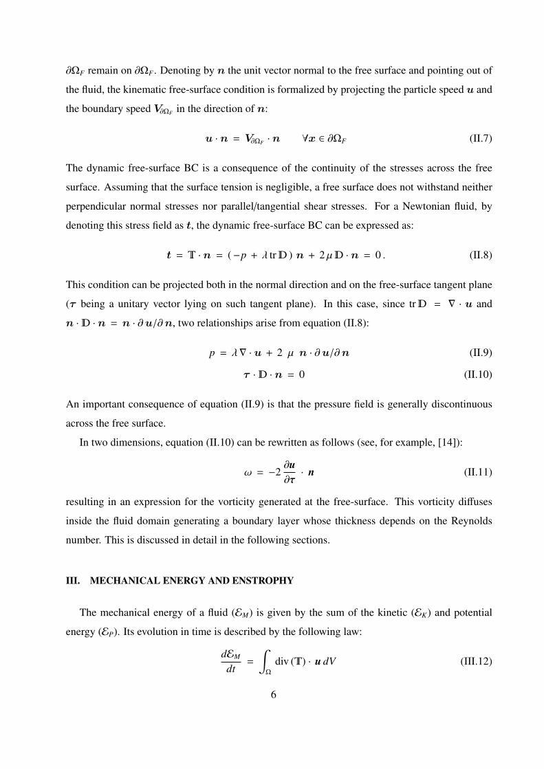
∂ΩF remain on ∂ΩF . Denoting by n the unit vector normal to the free surface and pointing out of

the fluid, the kinematic free-surface condition is formalized by projecting the particle speed u and

the boundary speed V∂ΩF in the direction of n:

u · n = V∂ΩF · n ∀x ∈ ∂ΩF (II.7)

The dynamic free-surface BC is a consequence of the continuity of the stresses across the free

surface. Assuming that the surface tension is negligible, a free surface does not withstand neither

perpendicular normal stresses nor parallel/tangential shear stresses. For a Newtonian fluid, by

denoting this stress field as t, the dynamic free-surface BC can be expressed as:

t = · n = (−p + λ tr ) n + 2 µ · n = 0 . (II.8)

This condition can be projected both in the normal direction and on the free-surface tangent plane

(τ being a unitary vector lying on such tangent plane). In this case, since tr = ∇ · u and

n · · n = n · ∂u/∂n, two relationships arise from equation (II.8):

p = λ∇ · u + 2 µ n · ∂u/∂n (II.9)

τ · · n = 0 (II.10)

An important consequence of equation (II.9) is that the pressure field is generally discontinuous

across the free surface.

In two dimensions, equation (II.10) can be rewritten as follows (see, for example, [14]):

ω = −2∂u∂τ· n (II.11)

resulting in an expression for the vorticity generated at the free-surface. This vorticity diffuses

inside the fluid domain generating a boundary layer whose thickness depends on the Reynolds

number. This is discussed in detail in the following sections.

III. MECHANICAL ENERGY AND ENSTROPHY

The mechanical energy of a fluid (EM) is given by the sum of the kinetic (EK) and potential

energy (EP). Its evolution in time is described by the following law:

dEM

dt=

∫Ω

div () · u dV (III.12)

6

Using the divergence theorem, the mechanical power on the boundary ∂Ω can be expressed as:∫∂Ω

(n · ) · u dS =

∫Ω

div( · u) dV =

∫Ω

div() · u dV +

∫Ω

: ∇u dV (III.13)

This power is zero on the free surface ∂ΩF since, by definition, an interface is said to be a free

surface when the tension τ = n · is null. Similarly, it is zero on the bottom ∂ΩB (which is

assumed here fixed) since the no-slip condition along solid bodies implies that u = 0. Using the

above considerations, equation (III.12) becomes:

dEM

dt= −

∫Ω

: dV (III.14)

where the velocity gradient has been replaced by its symmetric component since the tensor is

symmetric. For a Newtonian viscous fluid (see section II), equation (III.14) can be re-written as:

dEM

dt=

∫Ω

p div(u) dV − λ

∫Ω

[div(u)]2 dV − 2 µ∫

Ω

D : D dV (III.15)

In the analysis that follows, we define the different contributions as:

dEC

dt=

∫Ω

p div(u) dV ,dEB

dt= − λ

∫Ω

[div(u)]2 dV ,dED

dt= − 2 µ

∫Ω

D : D dV .

(III.16)

The energy EC represents the work associated with the fluid compressibility and is a pure reversible

energy. Using the equation of state and the continuity equation, EC can be reshaped as a potential

energy. The term EB represents the dissipation due to the fluid compressibility while ED is the

classical viscous term for a Newtonian fluid. If the fluid is weakly-compressible, EB can be

neglected. In fact, in all the numerical simulations that follow, it remains smaller than 0.1% of

the initial mechanical energy.

For an incompressible fluid, equation (III.15) reduces to:

dEM

dt=

dED

dt= − 2 µ

∫Ω

D : D dV (III.17)

Under the same hypothesis, substituting equation (II.3) in (III.12) the time variation of the

mechanical energy can be rewritten as:

dEM

dt=

∫Ω

−∇p · u dV + µ

∫Ω

∇2u · u dV , (III.18)

and, using the following identity (see, for example, [15]),

∇2u · u = div(u × ω) − |ω2| , (III.19)

7

it becomes:

dEM

dt=

∫Ω

−∇p · u dV − µ

∫∂Ω

(ω × u) · ndS − µ

∫Ω

|ω2| dV . (III.20)

Note that, because of the incompressibility of the fluid, it follows∫∂Ω

p u · ndS =

∫Ω

div(p u) dV =

∫Ω

∇p · u dV , (III.21)

and equation (III.20) can finally be rewritten as:

dEM

dt= −

∫∂Ω

p u · ndS − µ

∫∂Ω

(ω × u) · ndS − µ

∫Ω

|ω2| dV . (III.22)

Similarly to equation (III.15), we define the following contributions:

dE f p

dt= −

∫∂Ω

p u · ndS ,dE fω

dt= − µ

∫∂Ω

(ω × u) · ndS ,dEE

dt= − µ

∫Ω

|ω2| dV .

(III.23)

All these surface integrals are null at the bottom because of the no-slip condition whilst they

generally differ from zero along the free surface. The term EE is proportional to the enstrophy

(that is, to the rotational energy) and is always negative.

Equations (III.15) and (III.22) are used in the analysis of the numerical simulations, taking into

account the different energy contributions described above. Indeed, under certain conditions, we

show that the SPH model fails to converge to the expected solution and some of the contributions

defined in this section increase, inducing a non-physical attenuation of the wave amplitude.

Using the free-surface boundary conditions (II.9) and (II.11), equation (III.22) can be rewritten

as follows:dEM

dt= −2µ

∫∂ΩF

(∇u u) · ndS − µ

∫Ω

|ω2| dV . (III.24)

The above expression highlights the contribution on the rate of change of the mechanical energy

due to the flux of the convective acceleration (∇u u) on the free surface. The first term of (III.24)

may be extended to ∂Ω, since u is zero at the bottom. Note that, using the divergence theorem, we

can write:

∇ · (∇u u) = ∇(∇ · u) · u + ∇T u : ∇u = ∇(∇ · u) · u + D : D − |ω2|/2 (III.25)

For an incompressible fluid, the first term is zero and, consequently, it is possible to recover

equation (III.17).

8

IV. THE SPH MODEL

A. The SPH Regularized Navier-Stokes equations

The SPH model is based on the filtering (smoothing) of a generic flow field f through a

convolution integral with a kernel function W over the fluid domain Ω:

〈 f 〉(r) =

∫Ω

f (r′) W(r′ − r; h) dV ′ (IV.26)

where h is a measure of the kernel support and is generally called smoothing length. When h tends

to zero the kernel function W becomes a delta Dirac function. When this smoothing procedure is

applied to the differential operators of the governing equation (II.1), a regularized version of the

Navier-Stokes equations is obtained (see [16] for more details):

DρDt

= −ρ 〈∇ · u〉 ,

DuDt

= g −〈∇p〉ρ

+〈∇ ·〉

ρ,

DrDt

= u, p = c20 (ρ − ρ0)

(IV.27)

Following [2], the smoothed operators for the velocity and the pressure are:

〈∇ · u〉(r) =

∫Ω

[u(r′) − u(r)

]· ∇W(r′ − r) dV ′

〈∇p〉(r) =

∫Ω

[p(r′) + p(r)

]∇W(r′ − r) dV ′

(IV.28)

Assuming that the viscosity coefficients are constant across the fluid domain, the smoothed

operator for the viscous term is (see [13]):

〈∇ ·〉(r) = µK∫

Ω

[u(r′) − u(r)

]· (r′ − r)

|r′ − r|2∇W(r′ − r) dV ′ , (IV.29)

where the coefficient K is a parameter that depends on the spatial dimension (K = 6, 8, 10, in 1D,

2D and 3D respectively). A general discussion on the SPH viscous term can be found in [17].

The consistency of the system (IV.27) when h tends to zero has been deeply investigated in

[13] for viscous free-surface flows and in Macià et al.[18] for unidirectional flows with no-slip

boundary conditions along the solid boundaries. We underline that, the regularized equations

(IV.27) along with the differential operators in (IV.28) (IV.29) satisfy the free-surface boundary

conditions (II.9)-(II.10) in a weak sense (see, for example, [13]). Consequently, the free-surface

boundary conditions are not explicitly enforced in the SPH scheme.

9

B. Discretization of the governing equation

The SPH equations are obtained by discretizing the convolution integral inside equations

(IV.27):

Dρi

Dt= − ρi

∑j

(uj − uj

)· ∇Wi j ∆V j ,

Dui

Dt= g −

1ρi

∑j

(p j + pi)∇Wi j ∆V j + νK

∑j

[u j − ui

]· (r j − ri)

|r j − ri|2 ∇Wi j ∆V j ,

Dri

Dt= ui , pi = c2

0 (ρi − ρ0)

(IV.30)

Initially, particles are positioned on a Cartesian lattice with spacing ∆x and, consequently, their

volumes are ∆Vi = ∆x2. The velocity and pressure fields given as initial conditions come from

the analytical solution; the initial density field is deduced by using the equation of state. Thus, the

particle masses are mi = ρi ∆Vi. During the time evolution, mi does not change whilst the particle

volumes are updated through the density field, that is, ∆Vi(t) = mi/ρi(t). Finally, the ghost particles

method (see e.g. [19]) is used to enforce the boundary condition on the bottom.

Regarding the kernel function, we use the Wendland kernel ψ31 (see [20] for more details).

Such a kernel is positive defined and has continuous second derivatives. Hereinafter, we denote it

through WC2 and, following [21, 22], we renormalized it to obtain a compact support of radius

2h:

W(q) = β

(2 − q)4(1 + 2q) for 0 ≤ q ≤ 2

0 for q > 2. (IV.31)

Here, q = |r|/h while β is a normalization constant equal to 7/(64π) in 2D.

It is well documented in the SPH literature that the choice of the kernel function largely affects

the properties of the numerical scheme (see e.g [23–25]). The influence of this choice on the topic

addressed in this paper ( gravity waves attenuation SPH modeling ) is discussed in section VII C.

The convergence analysis for the SPH scheme has to be done by decreasing both the smoothing

length h and the spatial resolution ∆x. Specifically, the ratio h/∆x is proportional to the number

of neighbors interacting with a given particle (that is, to the number of particles in the kernel

domain). This ratio influences the accuracy of the discrete differential operators (see e.g. [26, 27])

and, consequently, the global properties of the scheme. Despite this, in the SPH literature, few

works focus on this topic which in turn mainly deal with inviscid flows (see e.g. [28], [29]) .

10

Error bounds of the interpolation procedure have been highlighted by Quinlan et al. [27] and

confirmed by Ellero et al. [30]. Specifically, Ellero et al. simulated the flow past a circular cylinder

with periodic boundary conditions at low Reynolds numbers. They investigated the convergence

rate of the drag coefficient and found, heuristically, that an increase of the spatial resolution does

not guarantee convergence unless the number of neighbors is above a certain limit.

Regarding this topic, it is important to underline that, in some practical applications, the

variability range of the parameter h/∆x can be very restricted, since numerical instabilities may

occur (for more details, see [31] and [32]).

The equations of system (IV.30) are marched in time using an explicit fourth-order Runge-Kutta

scheme. The global CFL of the integration scheme has to account for viscous diffusion, particle

acceleration ai, sound speed and particle velocity. The time-step bounds deriving from the first

two components have been modeled following Morris et al. [33]:

∆t1 ≤ 0.125h2

ν(IV.32)

∆t2 ≤ 0.25 mini

√h‖ai‖

(IV.33)

Usually, they depend very weakly on the specific integration scheme. The advective/acoustic

component is:

∆t ≤ CFL3 mini

(h

c0 + ‖ui‖

)(IV.34)

For a fourth-order Runge-Kutta scheme and for a Wendland kernel, we heuristically found

CFL3 = 2.2. The global CFL is given by the minimum of all the above bounds.

Since a fluid is generally characterized by a high sound speed, it is common practice in SPH

to use a numerical sound speed several orders of magnitude smaller than the physical one. In any

case, this numerical velocity has to be large enough to avoid compressibility effects. To make

them negligible, we set c0 = 10√

gH, as suggested in Madsen & Schäffer [34]. The validity of this

assumption is further verified in section VI.

Note that the numerical sound velocity is generally quite large and, if Re 1, the constrain

(IV.34) usually dominates over those in (IV.32) and (IV.33). Despite that, there always exists

a critical value of the smoothing length, say h∗, under which the constrain (IV.32) becomes

predominant. Below this value, the computational costs largely increase due to the quadratic

dependence of (IV.32) on the smoothing length.

11

V. ATTENUATION OF A STANDING WAVE

In the present section, we analyze in detail the phenomenon of viscous damping for gravity

waves. As explained in the introduction, we consider the evolution of a standing wave in order to

reduce the computational effort. An analytical solution of the linearized Navier-Stokes equation

(see formula (V.38) of the next section) has been used to evaluate the damping rate of the kinetic

energy and to check whether the SPH model is able to correctly predict the mechanical energy

decay. A further advantage of the standing wave is that the maximum wave steepness before

breaking is kA = 0.68 (here, A is the wave amplitude) while for propagative waves it is closer

to 0.45 (see [35]). This means that it is possible to inspect a wider range of wave steepnesses.

Remarkably, the analytical solution described in Section V A proved to be a reliable approximation

even for moderately high wave steepnesses (see section VII).

Figure 2 describes the initial configuration of the problem. Here, L is the wave length and

H = L/2 is the still water depth, the dimensionless wave number kH is therefore equal to π. Note

that the latter value means that the studied regime lies between deep (kH ≥ π) and intermediate

water conditions (π/10 ≤ kH < π). The free surface is initially flat in order to simplify particle

positioning. The initial value of the kinetic energy is computed and denoted as EK0. The initial

FIG. 2: Initial particle configuration, pressure and velocity fields for the standing wave problem.

12

pressure and velocity fields were evaluated using the analytical solution of Antuono & Colagrossi

[11].

As a first test case, we choose the nonlinearity parameter ε = 2A/H equal to 0.1 corresponding

to the steepness kA equal to π/20. The period of oscillation, T , is obtained through equation V.37

and depends on the Reynolds number chosen for the simulation (we recall that Re = H√

gH/ν).

Specifically, we chose five test cases with Re = 50, 250, 500, 2500, 5000. All simulations were

done assuming the fluid regime remains laminar. This is consistent with the analysis of Babanin

[36] which predicts that in similar conditions to the ones presented here, the critical Reynolds

number is close to 650, 000.

A. Approximate analytical solution for viscous gravity waves

To check the accuracy of the SPH scheme, we use an analytical solution of the linearized

Navier-Stokes equations for traveling waves.

The fluid variables are expressed through the following formulas:

u = U(y) eı θ + c.c. v = V(y) eı θ + c.c. (V.35)

p = P(y) eı θ + c.c. η = E eı θ + c.c. (V.36)

where u, v are the horizontal and vertical components of the velocity field, η is the free-surface

elevation, θ = k x − σ t and k is the wave number (i.e. k = 2π/L where L is the wave length).

Unlike the solution predicted by the inviscid theory, σ is a complex number: its real part represents

the circular frequency while the imaginary part gives the damping rate of the viscous gravity wave.

Substituting the expressions in (V.35) and (V.36) inside the linearized Navier-Stokes equations

and imposing the correct boundary conditions along the bottom and the free surface, it is possible

to obtain an implicit linear dispersion relation. Such a relation has been properly expanded in

13

series for ν 1 (where ν is the kinematic viscosity of the fluid):

<(σ) =√

g k tanh(kH) +

√2 (g ν2 k5)1/4

(tanh(kH)2 − 1

)4 tanh(kH)3/4 +

−

√2 (ν6 k11/g)1/4

(7 tanh(kH)6 + 147 tanh(kH)4 − 11 tanh(kH)2 − 15

)128 tanh(kH)13/4 + . . . (V.37)

=(σ) =

√2 (g ν2 k5)1/4

(tanh(kH)2 − 1

)4 tanh(kH)3/4 +

ν k2(tanh(kH)4 − 8 tanh(kH)2 − 1

)4 tanh(kH)2 +

+

√2 (ν6 k11/g)1/4

(7 tanh(kH)6 + 147 tanh(kH)4 − 11 tanh(kH)2 − 15

)128 tanh(kH)13/4 + . . . (V.38)

These expansions are well-posed for Re 1 and for Re−1 k Re2/3, where Re = H√

gH/ν is

the Reynolds number. The above bounds ensure that each term inside the perturbation expansion

is smaller than the preceding and larger than the subsequent for every value of k. The complex part

=(σ) is strictly negative and gives the dissipation rate of a viscous gravity wave propagating with

velocity<(σ)/k. As expected, the leading order of<(σ) coincides with the dispersion relation of

the potential theory while for the higher-orders, strictly negative terms appear. This means that the

viscosity tends to reduce the circular frequency and, consequently, the phase velocity of the wave.

Details of this analytical solution are reported in Antuono & Colagrossi [11].

Despite the linearized solution neglecting the advective terms inside the Navier-Stokes

equations, it adequately represents the global flow evolution as long as the nonlinearity parameter

ε stays small and the flow remains laminar. In fact, such hypotheses guarantee that the advective

terms are of order O(ε2).

B. Test matrix

To check the convergence of the SPH scheme, a matrix of 100 test cases has been considered.

The matrix has been organized as follows:

1. The range of Reynolds numbers (Re = 50, 250, 500, 2500, 5000) has been chosen broad

enough to describe different dissipation regimes.

2. For Re = 50, 250 and 500 the final time of the simulations (hereinafter t f ) has been chosen

large enough to reduce the kinetic energy to about 1% of its initial value. For Re = 2500 and

14

Re NT t f EK(t f )/EK0

50 4 14.2 0.0002

250 9 32.0 0.0103

500 16 56.8 0.0147

2500 25 88.8 0.2472

5000 28 99.4 0.4495

HHHH

HHHHH

h/∆xH/∆x 50 100 200 400 800

1 50 100 200 400 800

2 25 50 100 200 400

4 12.5 25 50 100 200

8 6.25 12.5 25 50 100

TABLE I: (Left) parameters of the simulations for the chosen Re. (Right) H/h values.

5000, this final time would imply too large computational costs due to the lower damping

rate. Therefore, in these cases the simulation time has been chosen long enough to allow for

a reasonable number of periods, NT , to take place.

3. For each Reynolds number, different spatial resolutions have been chosen. Specifically,

H/∆x = 50, 100, 200, 400, 800 with the corresponding number of particles being

5000, 20000, 80000, 320000 and 1280000 respectively.

4. h/∆x = 1, 2, 4, 8 in order to cover a realistic range of neighboring particles (respectively

8, 44, 200 and 800).

All these details are summarized in table I. Specifically, the right one contains the values of H/h

(representative of the smoothing level of the SPH modeling) as a function of H/∆x and h/∆x.

It is worth mentioning that a substantial computational effort was needed to run all these

simulations. A parallelized version of the code was used on a 30-CPU cluster, each CPU having 8

Xeon 2.33 GHz cores, running continuously for 30 days.

VI. VALIDATION OF THE SPH METHOD

A. Kinetic energy attenuation

In this section, the SPH scheme described in section IV is validated by studying the kinetic

energy decay for a viscous standing wave. The parameters of the problem, as well as those of the

SPH scheme, have been described in the previous sections.

The SPH kinetic energy is evaluated by a direct summation over the particles and its evolution

in time is compared with the analytical exponential decay of the kinetic energy described in section

15

V A. In agreement with the theoretical analysis of Colagrossi et al. [13] and for the highest values

of H/∆x and h/∆x, the SPH solution perfectly coincides with the analytical solution. These results

are reported in figures 3 to 5 for each Reynolds number along with the analytical damping rate.

Whilst for the lowest Reynolds number (Re = 50, left plot of figure 3) almost 98% of the energy

is attenuated after 2 periods, for the largest Reynolds number (Re = 5000, figure 5) and due to

the smaller viscosity, about 50% of the energy remains after 28 periods. This gives an idea of the

broad range of dissipation regimes considered in the present analysis.

B. Convergence of the SPH scheme

For the five Reynolds numbers considered, the convergence to the exact dissipation rate has

been investigated by inspecting the influence of the number of neighboring particles (h/∆x) and

the spatial resolution H/h. For each test case, an effective attenuation rate of the kinetic energy

has been obtained using a least square exponential fitting. Hereinafter, we will denote through

µ0 = 2=(σ) the analytical damping rate and by µ the damping rate predicted by the SPH scheme.

The SPH convergence to the analytical solution is achieved as both h/H and ∆x/h simultaneously

tend to zero. This is the case for all Reynolds numbers, as shown in figures 6 to 8.

For Re = 50, 250, 500 and for all h/∆x ratios (figure 6 and the left panel of figure 7), there is a

monotonic convergence to 1 of the µ/µ0 ratio when h goes to zero. Remarkably, the convergence

0.0 0.5 1.0 1.5 2.0 2.5 3.0 3.5 4.0

t/T

0.0

0.2

0.4

0.6

0.8

1.0

E K(t

)/E K

0

SPH

Analytical decay

0 1 2 3 4 5 6 7 8 9

t/T

0.0

0.2

0.4

0.6

0.8

1.0

E K(t

)/E K

0

SPH

Analytical decay

FIG. 3: Kinetic energy decay. Left: Re = 50, h/∆x = 4, H/∆x = 800. Right: Re = 250, h/∆x = 4,

H/∆x = 800.

16

0 2 4 6 8 10 12 14 16

t/T

0.0

0.2

0.4

0.6

0.8

1.0E K

(t)/E K

0SPH

Analytical decay

0 5 10 15 20 25

t/T

0.0

0.2

0.4

0.6

0.8

1.0

E K(t

)/E K

0

SPH

Analytical decay

FIG. 4: Kinetic energy decay. Left: Re = 500, h/∆x = 2, H/∆x = 800. Right: Re = 2500, h/∆x = 4,

H/∆x = 800.

0 5 10 15 20 25

t/T

0.0

0.2

0.4

0.6

0.8

1.0

E K(t

)/E K

0

SPH

Analytical decay

FIG. 5: Kinetic energy decay: Re = 5000, h/∆x = 4, H/∆x = 800.

is attained even when using only 8 neighboring particles (that is, for h/∆x = 1). As expected, the

convergence rate increases as h/∆x becomes larger and larger.

For Re = 2500 (right plot of figure 7), the convergence is lost for h/∆x = 1 while for h/∆x = 2

the SPH method seems to converge to a value that is slightly different from the analytical one.

Similarly, for Re = 5000 (figure 8), the case with h/∆x = 1 provides inaccurate results while for

h/∆x = 2 the damping rate is largely overestimated.

For small values of h/∆x and high Reynolds numbers, the failure to converge may be hastily

17

attributed to the lack of a fine enough spatial resolution to model the boundary layers. Indeed,

for high Reynolds numbers, the vorticity is mainly concentrated in these thin layers of fluid

whose thickness, δBL, is inversely proportional to the square root of Re [37] (see table II). Then,

if the spatial resolution of the SPH scheme is too coarse, the dissipation rate may be wrongly

estimated. Unfortunately, the dissipative phenomenon is also badly represented in those test cases

characterized by a very fine discretization. This is briefly described in figure 9 where the test cases

100

101

102

103

0.95

1

1.05

1.1

1.15

H/h

/ 0

h/x=1h/x=2h/x=4h/x=8

100

101

102

103

1

1.1

1.2

1.3

1.4

H/h

/ 0

h/x=1h/x=2h/x=4h/x=8

FIG. 6: Convergence analysis of the µ/µ0 ratio; left: Re = 50, right: Re = 250.

100

101

102

103

1

1.2

1.4

1.6

H/h

/ 0

h/x=1h/x=2h/x=4h/x=8

100

101

102

103

1

1.5

2

H/h

/ 0

h/x=1h/x=2h/x=4h/x=8

FIG. 7: Convergence analysis of the µ/µ0 ratio; left: Re = 500, right: Re = 2500.

100

101

102

103

1

1.5

2

2.5

3

3.5

H/h

/ 0

h/x=1h/x=2h/x=4h/x=8

FIG. 8: Convergence analysis of the µ/µ0 ratio, Re = 5000.

18

Re 50 250 500 2500 5000

δBL/H 0.14 0.06 0.04 0.02 0.01

TABLE II: Thickness of the free-surface boundary layer as a function of Re (see [37]).

characterized by δBL/h between 3 and 5 have been selected. Although the boundary layers are

well discretized, the ratio µ/µ0 for h/∆x = 2 diverges as Re increases. This means that, even if the

free surface boundary layer is properly resolved, an increase of h/∆x is still necessary in order to

maintain an equivalent accuracy as Re increases. In the next sections we try to better address this

issue.

101

102

103

104

1

1.5

2

2.5

3

Re

/ 0

h/x=1h/x=2h/x=4h/x=8

FIG. 9: Attenuation ratio as a function of Re and h/∆x (3 ≤ δBL/h ≤ 5).

C. Analysis of the dissipation components

Figure 10 displays the evolution of the kinetic energy for Re = 5000 and h/∆x = 2, 4.

Specifically, for h/∆x = 2 the SPH model predicts an over damping of the wave energy when

compared to the theoretical decay. For the present analysis, it is of fundamental importance to

understand the cause of such an extra dissipation.

In section III, the mechanical energy variation has been divided into three contributions,

EB,EC,ED [see equation (III.15)]. Specifically, EB is negligible since it remains smaller than

0.1% of the initial kinetic energy, EK0, while EC is sensibly different from zero and is related to

the fluid compressibility. The last contribution, that is ED, represents the classical dissipative term

19

0 5 10 15 20 25

t/T

0.0

0.2

0.4

0.6

0.8

1.0

E K(t

)/E K

0

h/∆x = 2

h/∆x = 4

Analytical decay

0 5 10 15 20 25

t/T

−0.05

0.00

0.05

0.10

0.15

E C(t

)/E K

0

h/∆x = 2

h/∆x = 4

FIG. 10: Evolution in time of the kinetic energy (top panel) and of the pressure term EC (bottom panel) for

Re = 5000, H/∆x = 800 and h/∆x = 2, 4.

for incompressible Newtonian flows.

First, we focus on EC and check whether it may be the cause of the reduced accuracy of the

SPH scheme. In the bottom plot of figure 10, the evolution time of EC is shown for h/∆x = 2, 4

and Re = 5000. Both time series consist of high frequency (namely, ' c0/2/L) components that

oscillate around a constant mean value (EC being a pure reversible energy). Since the mean value

does not exceed 5% of the initial kinetic energy, we conclude that the weakly compressibility

nature of the numerical scheme does not justify the large differences observed in the top plot of

figure 10. We therefore deduce that the cause of the unphysical over-damping is due to the term

ED.

Using equations (III.17) and (III.24), it is possible to express ED as a sum of three contributions:

a free-surface pressure term, E f p, a free-surface vorticity term, E fω and an enstrophy volume

integral, EE.

Figure 11 displays the vorticity field for h/∆x = 4, H/∆x = 800 and Re = 5000 at two

20

representative instants of the simulation. As shown in figure 10, this case accurately predicts the

attenuation rate. The vorticity field is smooth and characterized by high gradients close to the

free-surface boundary layer while being practically zero inside the bulk of the fluid.

FIG. 11: Vorticity field for h/∆x = 4, H/∆x = 800 and Re = 5000 at t/T = 4.5 (left panel) and t/T = 16.5

(right panel).

In figure 12, the vorticity field is drawn at the same time instants for h/∆x = 2, H/∆x = 800

and Re = 5000. In this case and after a few periods, spurious vorticity appears in the bulk of the

fluid with an intensity comparable to the vorticity enclosed in the free-surface boundary layer. As

the simulation goes on (right plot of figure 12), these spurious vortical structures occupy an ever

growing part of the fluid domain.

The areas where the vorticity instabilities first occur are characterized by the largest velocities

and particle displacements. In these regions the initial Cartesian lattice is greatly deformed

and numerical errors induce a rearrangement of the particle positions which causes the spurious

vorticity spots. Instabilities in the vorticity field also appear close to the free surface, possibly

caused by the interpolation errors related to the kernel truncation (see e.g. [2]).

Figure 13 shows some details of these vorticity spots. Remarkably, no particle disorder is

associated with these structures. This phenomenon is closely related to the development of

spurious vorticity discussed in Ellero et al.[38], where a similar study was performed on a steady

shear flow. Due to the unsteadiness nature of the viscous standing wave and to the presence of

21

FIG. 12: Vorticity field for h/∆x = 2, H/∆x = 800 and Re = 5000 at t/T = 4.5 (left panel) and t/T = 16.5

(right panel).

FIG. 13: Details of the vorticity field for h/∆x = 2, H/∆x = 800 and Re = 5000 at t/T = 4.5 (left panel)

and t/T = 16.5 (right panel).

free-surface dynamics, it has not been possible to follow the analysis of that work.

The spurious vorticity generated when h/∆x = 2 mainly affects the enstrophy integral, EE. The

contributions E f p,E fω and EE defined in equation III.24 are displayed in figure 14. The surface

integral terms, namely(E f p + E fω

), are displayed in the left plot of figure 14. The agreement with

the analytical solution is good for h/∆x = 4 while some discrepancies arise for a smaller number

22

0 5 10 15 20 25

t/T

0.4

0.5

0.6

0.7

0.8

0.9

1.0(Efp(t

)+E f

ω(t

))/E

K0

+1 h/∆x = 2

h/∆x = 4

Analytical solution

0 5 10 15 20 25

t/T

0.84

0.86

0.88

0.90

0.92

0.94

0.96

0.98

1.00

E E(t

)/E K

0+

1

h/∆x = 2

h/∆x = 4

Analytical solution

FIG. 14: Standing wave with Re = 5000, H/∆x = 800 and h/∆x = 2, 4. Left: surface integral terms,(E f p + E fω

). Right: enstrophy contribution, EE .

FIG. 15: Dynamic pressure field (Re = 5000) at t/T = 4.5 (H/∆x = 800). Left panel: h/∆x = 2. Right

panel: h/∆x = 4.

of neighboring particles (h/∆x = 2). The evolution of EE, that is, the volume integral of the

enstrophy, is shown in the right plot of figure 14. When the spurious generation of vorticity occurs

(as is the case for h/∆x = 2), EE largely deviates from the analytical solution and is responsible

for the largest part of the extra dissipation.

The analytical solution plotted in figure 14 highlights the fact that the main dissipation

mechanism is mainly due to the surface term of equation (III.24) rather than the enstrophy term.

This is a peculiarity of gravity waves in deep water condition, since in intermediate and shallow

water conditions the enstrophy becomes increasingly relevant due to the dynamics of the bottom

boundary layer. This is briefly shown in section VII A.

23

When the instabilities on the vorticity field occur, spurious pressure forces develop inducing

spurious particle motions (see figure 15). In all the cases described in the present work, the

pressure term F pi = (∇p/ρ)i dominates the viscous one, namely Fv

i = µ(∇2u/ρ)i. In any case, the

action in time of the viscous term is non-negligible since it causes the mechanical energy decay.

Conversely, as shown in this section, the energy components due to the weakly-compressible

assumption, namely EB and EC, remain negligible even when the scheme becomes unstable.

This means that this kind of numerical instabilities is likely due to the particulate nature of

the method rather than the use of a specific equation of state. This statement is coherent with

the Moving Particle Semi-Implicit (MPS) method simulations of the attenuation of a standing

wave documented in [39], where over-damping is also present. The MPS method is a meshless

numerical technique [40, 41] used to solve incompressible Navier-Stokes equations. In order for

the obtained flow field to exhibit the properties of an incompressible flow, a fractional time step

approach is used. As discussed in [39], the MPS method is closely related to SPH in general and

to incompressible SPH in particular, due to the technique used to impose incompressibility.

VII. ADDITIONAL REMARKS

A. Influence of the wave number

In the present section we show that the results described until now are still valid when different

wave numbers are considered. Specifically, we chose kH = 2π (deep water) and kH = π/2

(intermediate water) and limited the analysis to the most challenging case, that is, Re = 5000.

The nonlinearity parameter ε = 2A/H is maintained equal to 0.1 as in the previous test cases.

For kH = 2π the standing wave dynamics intensify and after 30 periods about 80% of the kinetic

energy is dissipated. Conversely, for kH = π/2 the same result would be obtained after 320 periods

of evolution. The spatial resolution is the same for both cases, that is, H/∆x = 800, meaning that

the test case where kH = π/2 requires about 2.5 million particles. Because of this huge number

of particles and of the slower dynamics, it was only possible to simulate 7 periods of oscillation

for kH = π/2. In any case, this interval is long enough for the proposed analysis. Similarly

to the results described in the previous section, in both cases, spurious vorticity is generated for

h/∆x = 2 (left panels of figot me ures 16 and 17) leading to an over-damping of the kinetic energy

(see figure 18). For kH = 2π, the over-damping is limited to a few percent and is visible after

24

FIG. 16: Vorticity field for kH = 2π, Re = 5000, H/∆x = 800. Left: h/∆x = 2. Right: h/∆x = 4.

FIG. 17: Vorticity field for kH = π/2, Re = 5000, H/∆x = 800. Top: h/∆x = 2. Bottom: h/∆x = 4.

only 20 periods whilst for kH = π/2 a larger energy decay appears after just a few periods of

the evolution. Again, when using h/∆x = 4 the spurious vorticity field disappears and the SPH

solution regains a good agreement with the analytical one. Note that for kH = π/2 the dynamics

of the bottom boundary layer are quite strong (see bottom panel of figure 17) and play a relevant

25

0 5 10 15 20 25 30

t/T

0.0

0.2

0.4

0.6

0.8

1.0E K

(t)/E K

0h/∆x = 2

h/∆x = 4

Analytical decay

0 1 2 3 4 5 6

t/T

0.0

0.2

0.4

0.6

0.8

1.0

1.2

1.4

1.6

E K(t

)/E K

0

h/∆x = 2

h/∆x = 4

Analytical decay

FIG. 18: Kinetic energy for Re = 5000, H/∆x = 800. Left: kH = 2π. Right: kH = π/2.

role in the dissipation mechanisms.

B. Influence of the wave amplitude

Here, we inspect the influence of the variation of the wave amplitude on the dissipation

mechanisms. The dimensionless wave amplitude, ε = 2A/H, is reduced to 0.002 (note that in

all previous tests cases ε = 0.1). Figure 19 displays the kinetic energy evolution for Re = 500,

h/∆x = 2 and H/∆x = 400. Similarly to the case where ε = 0.1, no over-damping is detected even

if the SPH signal is disturbed by high-frequency oscillations caused by the fluid compressibility.

As a second example, we choose a large amplitude wave characterized by ε = 0.4, In this case,

the wave steepness is kA = 0.628 and therefore very close to the breaking limit 0.68 (see [35]).

Hence, this case is characterized by high non-linearities, especially close to the free surface (see

left plot of figure 20). Nonetheless, the agreement with the linear solution (section V A) is still

good (see the right plot of figure 20). This is a clear indication that the linearized Navier-Stokes

solution provides a good estimation of the energy attenuation even for high wave steepnesses.

0 2 4 6 8 10 12 14 16

t/T

0.0

0.2

0.4

0.6

0.8

1.0

E K(t

)/E K

0

ε = 0.1

ε = 0.002

Analytical decay

FIG. 19: Kinetic energy for different wave amplitudes (Re = 500, h/∆x = 2, H/∆x = 400).

26

0 2 4 6 8 10 12 14 16

t/T

0.0

0.2

0.4

0.6

0.8

1.0

E K(t

)/E K

0

SPH

Analytical decay

FIG. 20: Large amplitude case: ε = 0.4, Re = 500, h/∆x = 2, H/∆x = 400. Left: vorticity field. Right:

kinetic energy decay.

C. Effects of the kernel choice for Re = 5000

As a final part of the analysis, we inspect the influence of the kernel choice on the gravity wave

simulations. Specifically, we focus on the test cases where Re = 5000.

As shown in section VI B, the damping rate computed using the Wendland kernel does not

converge for H/∆x = 800 and h/∆x = 2 (figures 10 and 12). This simulation has been repeated

using a Renormalized Gaussian Kernel (hereinafter RGK). In the SPH literature[23], the radius of

the RGK is set equal to 3h. However, to allow a comparison with the Wendland kernel, its radius

has been rescaled to 2h:

WRGK(q) = Mα

exp(−α2 q2) − mα for 0 ≤ q ≤ 2

0 for q > 2(VII.39)

where α = 3/2, M3/2 = 0.717082 and m3/2 = exp(−9).

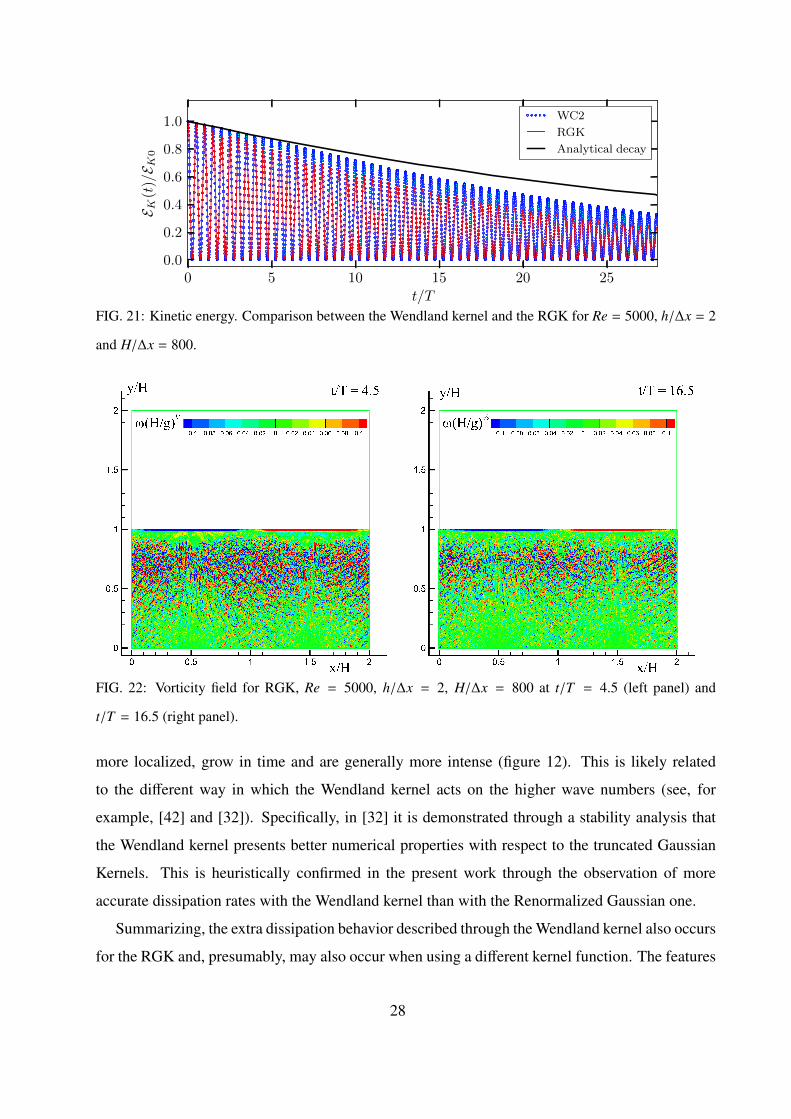
Figure 21 clearly shows that, in comparison to the Wendland kernel, the use of the RGK leads

to a larger over-damping process. Similarly to what was done for the Wendland kernel, we focus

on the evolution of the vorticity field. Figure 22 displays the vorticity field predicted by SPH

with the RGK at t = 4.5T and t = 16.5T . In the early phase of the simulation, a significant

amount of spurious vorticity is generated across the fluid domain and remains almost unchanged

throughout the process. On the contrary, the vorticity structures displayed using the WC2 are

27

0 5 10 15 20 25

t/T

0.0

0.2

0.4

0.6

0.8

1.0

E K(t

)/E K

0

WC2

RGK

Analytical decay

FIG. 21: Kinetic energy. Comparison between the Wendland kernel and the RGK for Re = 5000, h/∆x = 2

and H/∆x = 800.

FIG. 22: Vorticity field for RGK, Re = 5000, h/∆x = 2, H/∆x = 800 at t/T = 4.5 (left panel) and

t/T = 16.5 (right panel).

more localized, grow in time and are generally more intense (figure 12). This is likely related

to the different way in which the Wendland kernel acts on the higher wave numbers (see, for

example, [42] and [32]). Specifically, in [32] it is demonstrated through a stability analysis that

the Wendland kernel presents better numerical properties with respect to the truncated Gaussian

Kernels. This is heuristically confirmed in the present work through the observation of more

accurate dissipation rates with the Wendland kernel than with the Renormalized Gaussian one.

Summarizing, the extra dissipation behavior described through the Wendland kernel also occurs

for the RGK and, presumably, may also occur when using a different kernel function. The features

28

of the over-damping process are obviously related to the specific kernel adopted but are likely

influenced by the ratio h/∆x.

VIII. CONCLUSIONS

The attenuation of a viscous standing wave has been studied using the Smoothed Particle

Hydrodynamics model in its original weakly compressible version. A broad range of Reynolds

numbers has been considered and the convergence of the numerical scheme has been checked

by varying the spatial resolution as well as the number of neighboring particles. A solution of

the linearized Navier-Stokes equation over finite depths has been used as benchmark for the SPH

results.

It has been shown that the kinetic energy attenuation predicted by the SPH scheme generally

shows a good agreement with the analytical solution as the spatial resolution and number of

neighbors increase. Specifically, it has been shown that for higher Reynolds numbers more

neighboring particles are needed in order to correctly model the dissipation.

Over-attenuation of the wave has been observed in some cases; it has been shown that such

an extra dissipation does not come from the weak compressibility of the numerical model but

is strictly related to a spurious growth of the enstrophy. In these cases, large spurious vorticity

develops inside the bulk of fluid.

Three additional topics have been considered, namely, the influence of the wave amplitude,

wave number and kernel choice in the attenuation rate. The former two do not affect the results

while the kernel choice has a significant influence on the evolution of the dissipation contributions.

Future works will be addressed to clarify the main mechanism which leads to the generation of

spurious vorticity for high Reynolds numbers. The influence of the kernel choice also remains an

open problem.

Acknowledgments

The research leading to these results has received funding by the Flagship Project RITMARE

- The Italian Research for the Sea - coordinated by the Italian National Research Council and

funded by the Italian Ministry of Education, University and Research within the National Research

Program 2011-2013 and by the Spanish Ministry for Science and Innovation under the grant

29

TRA2010-16988 “Caracterización Numérica y Experimental de las Cargas Fluido-Dinámicas en

el transporte de Gas Licuado”. This work was also partially supported by the Centre of Excellence

CeSOS/CAMOS, NTNU, Norway.

The authors thank Marco Ellero from TUM and Andrea di Mascio from IAC in Rome for their

inspiration during the initial part of the research presented in this paper. Finally, the authors are

grateful to Hugo Gee for the correction and improvement of the English text.

[1] L. M. Sun and Y. Fujino, Journal of Fluids and Structures 8, 471 (1994).

[2] A. Colagrossi, M. Antuono, and D. L. Touzé, Physical Review E (Statistical, Nonlinear, and Soft

Matter Physics) 79, 056701 (pages 13) (2009).

[3] F. H. Harlow and J. E. Welch, Physics of Fluids 8, 2182 (1965).

[4] E. Haddon and N. Riley, Wave Motion 5, 43 (1983), ISSN 0165-2125, URL http://www.

sciencedirect.com/science/article/pii/0165212583900057.

[5] P. L.-F. Liu and A. Orfila, Journal of Fluid Mechanics 520, 83 (2004), URL http://dx.doi.org/

10.1017/S0022112004001806.

[6] A. Raval, X. Wen, and M. H. Smith, Journal of Fluid Mechanics 637, 443 (2009), URL http:

//dx.doi.org/10.1017/S002211200999070X.

[7] M. Basa, N. J. Quinlan, and M. Lastiwka, International Journal for Numerical Methods in Fluids 60,

1127 (2009).

[8] F. Macià, J. M. Sánchez, A. Souto-Iglesias, and L. M. González, International Journal for Numerical

Methods in Fluids 69, 509 (2012), ISSN 1097-0363.

[9] A. Valizadeh and J. J. Monaghan, Physics of Fluids 24, 035107 (pages 18) (2012), URL http:

//link.aip.org/link/?PHF/24/035107/1.

[10] M. Antuono, A. Colagrossi, S. Marrone, and C. Lugni, Computer Physics Communications

182, 866 (2011), ISSN 0010-4655, URL http://www.sciencedirect.com/science/article/

B6TJ5-51PRYCS-1/2/b69f4a14370f08b80c197c90035b226a.

[11] M. Antuono and A. Colagrossi, Wave Motion pp. – (2012), ISSN 0165-2125, URL http://www.

sciencedirect.com/science/article/pii/S0165212512001060.

[12] J. Lighthill, Waves in fluids (Cambridge University Press, 2001).

[13] A. Colagrossi, M. Antuono, A. Souto-Iglesias, and D. Le Touzé, Physical Review E 84, 26705+

30

(2011).

[14] T. Lundgren and P. Koumoutsakos, Journal of Fluid Mechanics 382, 351 (1999), URL http:

//dx.doi.org/10.1017/S0022112098003978.

[15] A. Iafrati, Journal of Fluid Mechanics 622, 371 (2009), URL http://dx.doi.org/10.1017/

S0022112008005302.

[16] J. J. Monaghan, Reports on Progress in Physics 68, 1703 (2005).

[17] D. Violeau, Phys. Rev. E 80, 036705 (2009), URL http://link.aps.org/doi/10.1103/

PhysRevE.80.036705.

[18] F. Maciá, M. Antuono, L. M. González, and A. Colagrossi, Progress of Theoretical Physics 125, 1091

(2011), URL http://ptp.ipap.jp/link?PTP/125/1091/.

[19] A. Colagrossi and M. Landrini, J. Comp. Phys. 191, 448 (2003).

[20] H. Wendland, Adv. Comput. Math. 4, 389 (1995), ISSN 1019-7168, URL http://dx.doi.org/10.

1007/BF02123482.

[21] M. Robinson and J. Monaghan, in 3rd ERCOFTAC SPHERIC workshop on SPH applications (2008),

pp. 78–84.

[22] M. Robinson, Ph.D. thesis, Department of Mathematical Science, Monash University (2009).

[23] D. Molteni and A. Colagrossi, Computer Physics Communications 180, 861 (2009).

[24] J. Hongbin and D. Xin, Journal of Computational Physics 202, 699 (2005), ISSN

0021-9991, URL http://www.sciencedirect.com/science/article/B6WHY-4D98HF9-2/2/

d14f8e7073f8e75148d766a8623e9af3.

[25] J. Morris, Ph.D. thesis, Mathematics Department, Monash University, Melbourne, Australia (1996).

[26] S. Mas-Gallic and P. A. Raviart, Numerische Mathematik 51, 323 (1987), ISSN 0029-599X,

10.1007/BF01400118, URL http://dx.doi.org/10.1007/BF01400118.

[27] N. J. Quinlan, M. Lastiwka, and M. Basa, International Journal for Numerical Methods in Engineering

66, 2064 (2006), URL http://dx.doi.org/10.1002/nme.1617.

[28] R. Di Lisio, E. Grenier, and M. Pulvirenti, Computers and Mathematics with Applications 35, 95

(1998).

[29] B. M. B and J. Vila, SIAM Journal on Numerical Analysis 37 (3), 863 (2000).

[30] M. Ellero and N. A. Adams, International Journal for Numerical Methods in Engineering 86, 1027

(2011), ISSN 1097-0207, URL http://dx.doi.org/10.1002/nme.3088.

[31] J. W. Swegle, D. L. Hicks, and S. W. Attaway, Journal of Computational Physics 116, 123 (1995).

31

[32] W. Dehnen and H. Aly, Monthly Notices of the Royal Astronomical Society 425, 1068 (2012), ISSN

1365-2966, URL http://dx.doi.org/10.1111/j.1365-2966.2012.21439.x.

[33] J. P. Morris, P. J. Fox, and Y. Zhu, Journal of Computational Physics 136, 214 (1997).

[34] P. Madsen and H. Schäffer, Coastal Engineering 53, 93 (2006), ISSN 0378-3839, URL http:

//www.sciencedirect.com/science/article/pii/S0378383905001250.

[35] R. Dean and R. Dalrymple, Water wave mechanics for engineers and scientists, Advanced series on

ocean engineering (World Scientific, 1991), ISBN 9789810204211, URL http://books.google.

es/books?id=9-M4U\_sfin8C.

[36] A. V. Babanin, Geophysical Research Letters 33, L20605+ (2006), ISSN 0094-8276, URL http:

//dx.doi.org/10.1029/2006GL027308.

[37] A.-K. Liu and S. H. Davis, Journal of Fluid Mechanics 81, 63 (1977), URL http://dx.doi.org/

10.1017/S0022112077001918.

[38] M. Ellero, P. Español, and N. A. Adams, Phys. Rev. E 82, 046702 (2010).

[39] A. Souto-Iglesias, F. Macià, L. M. González, and J. L. Cercos-Pita, Computer Physics

Communications pp. – (2012), ISSN 0010-4655, URL http://www.sciencedirect.com/

science/article/pii/S0010465512003852?v=s5.

[40] A. Khayyer and H. Gotoh, Applied Ocean Research 37, 120 (2012), ISSN 0141-1187, URL

http://www.sciencedirect.com/science/article/pii/S0141118712000399.

[41] M. M. Tsukamoto, L.-Y. Cheng, and K. Nishimoto, Computers & Fluids 49, 1 (2011), ISSN 0045-

7930, URL http://www.sciencedirect.com/science/article/pii/S0045793011001423.

[42] F. Macià, A. Colagrossi, M. Antuono, and A. Souto-Iglesias, in 6th ERCOFTAC SPHERIC workshop

on SPH applications (2011).

32