Review Hydrodynamics and phases of flocks
75
Review Hydrodynamics and phases of flocks John Toner a , Yuhai Tu b, * , Sriram Ramaswamy c a Institute of Theoretical Science, Department of Physics, University of Oregon, Eugene, OR 97403-5203, USA b IBM T. J. Watson Research Center, P.O. Box 218, Yorktown Heights, NY 10598, USA c Centre for Condensed Matter Theory, Department of Physics, Indian Institute of Science, Bangalore 560012, India Received 18 March 2005; accepted 4 April 2005 Abstract We review the past decadeÕs theoretical and experimental studies of flocking: the collective, coherent motion of large numbers of self-propelled ‘‘particles’’ (usually, but not always, living organisms). Like equilibrium condensed matter systems, flocks exhibit distinct ‘‘phases’’ which can be classified by their symmetries. Indeed, the phases that have been theoretically studied to date each have exactly the same symmetry as some equilibrium phase (e.g., ferromagnets, li- quid crystals). This analogy with equilibrium phases of matter continues in that all flocks in the same phase, regardless of their constituents, have the same ‘‘hydrodynamic’’—that is, long-length scale and long-time behavior, just as, e.g., all equilibrium fluids are described by the Navier–Stokes equations. Flocks are nonetheless very different from equilibrium sys- tems, due to the intrinsically nonequilibrium self-propulsion of the constituent ‘‘organisms.’’ This difference between flocks and equilibrium systems is most dramatically manifested in the ability of the simplest phase of a flock, in which all the organisms are, on average moving in the same direction (we call this a ‘‘ferromagnetic’’ flock; we also use the terms ‘‘vector-or- dered’’ and ‘‘polar-ordered’’ for this situation) to exist even in two dimensions (i.e., creatures moving on a plane), in defiance of the well-known Mermin–Wagner theorem of equilibrium statistical mechanics, which states that a continuous symmetry (in this case, rotation invari- ance, or the ability of the flock to fly in any direction) can not be spontaneously broken in a two-dimensional system with only short-ranged interactions. The ‘‘nematic’’ phase of flocks, www.elsevier.com/locate/aop Annals of Physics 318 (2005) 170–244 0003-4916/$ - see front matter Ó 2005 Elsevier Inc. All rights reserved. doi:10.1016/j.aop.2005.04.011 * Corresponding author. E-mail address: [email protected] (Y. Tu).
Transcript of Review Hydrodynamics and phases of flocks
www.elsevier.com/locate/aop
Annals of Physics 318 (2005) 170–244
Review
Hydrodynamics and phases of flocks
John Toner a, Yuhai Tu b,*, Sriram Ramaswamy c
a Institute of Theoretical Science, Department of Physics, University of Oregon, Eugene,
OR 97403-5203, USAb IBM T. J. Watson Research Center, P.O. Box 218, Yorktown Heights, NY 10598, USA
c Centre for Condensed Matter Theory, Department of Physics,
Indian Institute of Science, Bangalore 560012, India
Received 18 March 2005; accepted 4 April 2005
Abstract
We review the past decade�s theoretical and experimental studies of flocking: the collective,coherent motion of large numbers of self-propelled ‘‘particles’’ (usually, but not always, livingorganisms). Like equilibrium condensed matter systems, flocks exhibit distinct ‘‘phases’’ whichcan be classified by their symmetries. Indeed, the phases that have been theoretically studied todate each have exactly the same symmetry as some equilibrium phase (e.g., ferromagnets, li-quid crystals). This analogy with equilibrium phases of matter continues in that all flocks inthe same phase, regardless of their constituents, have the same ‘‘hydrodynamic’’—that is,long-length scale and long-time behavior, just as, e.g., all equilibrium fluids are describedby the Navier–Stokes equations. Flocks are nonetheless very different from equilibrium sys-tems, due to the intrinsically nonequilibrium self-propulsion of the constituent ‘‘organisms.’’This difference between flocks and equilibrium systems is most dramatically manifested inthe ability of the simplest phase of a flock, in which all the organisms are, on average movingin the same direction (we call this a ‘‘ferromagnetic’’ flock; we also use the terms ‘‘vector-or-dered’’ and ‘‘polar-ordered’’ for this situation) to exist even in two dimensions (i.e., creaturesmoving on a plane), in defiance of the well-known Mermin–Wagner theorem of equilibriumstatistical mechanics, which states that a continuous symmetry (in this case, rotation invari-ance, or the ability of the flock to fly in any direction) can not be spontaneously broken ina two-dimensional system with only short-ranged interactions. The ‘‘nematic’’ phase of flocks,
0003-4916/$ - see front matter � 2005 Elsevier Inc. All rights reserved.
doi:10.1016/j.aop.2005.04.011
* Corresponding author.E-mail address: [email protected] (Y. Tu).

J. Toner et al. / Annals of Physics 318 (2005) 170–244 171
in which all the creatures move preferentially, or are simply oriented preferentially, along thesame axis, but with equal probability of moving in either direction, also differs dramaticallyfrom its equilibrium counterpart (in this case, nematic liquid crystals). Specifically, it showsenormous number fluctuations, which actually grow with the number of organisms faster thanthe
ffiffiffiffiN
p‘‘law of large numbers’’ obeyed by virtually all other known systems. As for equilib-
rium systems, the hydrodynamic behavior of any phase of flocks is radically modified by addi-tional conservation laws. One such law is conservation of momentum of the background fluidthrough which many flocks move, which gives rise to the ‘‘hydrodynamic backflow’’ inducedby the motion of a large flock through a fluid. We review the theoretical work on the effect ofsuch background hydrodynamics on three phases of flocks—the ferromagnetic and nematicphases described above, and the disordered phase in which there is no order in the motionof the organisms. The most surprising prediction in this case is that ‘‘ferromagnetic’’ motionis always unstable for low Reynolds-number suspensions. Experiments appear to have seenthis instability, but a quantitative comparison is awaited. We conclude by suggesting furthertheoretical and experimental work to be done.� 2005 Elsevier Inc. All rights reserved.
1. Introduction
Flocking [1]—the collective, coherent motion of large numbers of organisms—isone of the most familiar and ubiquitous biological phenomena. We have all seenflocks of birds, schools of fish, herd of wildebeest, etc. (at least on film). We will here-after refer to all such collective motions—flocks, swarms, herds, etc.—as ‘‘flocking.’’This phenomenon also spans an enormous range of length scales: from kilometers(herds of wildebeest) to micrometers (e.g., the micro-organism Dictyostelium discoid-eum) [2–4]. Remarkably, despite the familiarity and widespread nature of the phe-nomenon, it is only in the last 10 years or so that many of the universal featuresof flocks have been identified and understood. It is our goal in this paper to reviewthese recent developments, and to suggest some of the directions future research onthis subject could take.
This ‘‘modern era’’ in the understanding of flocks began with the work of Vicseket al. [5], who was, to our knowledge, the first to recognize that flocks fall into thebroad category of nonequilibrium dynamical systems with many degrees of freedomthat has, over the past few decades, been studied using powerful techniques origi-nally developed for equilibrium condensed matter and statistical physics (e.g., scal-ing, the renormalization group, etc.). In particular, Vicsek noted an analogybetween flocking and ferromagnetism: the velocity vector of the individual birds islike the magnetic spin on an iron atom in a ferromagnet. The usual ‘‘moving phase’’of a flock, in which all the birds, on average, are moving in the same direction, is thenthe analog of the ‘‘ferromagnetic’’ phase of iron, in which all the spins, an average,point in the same direction. Another way to say this is that the development of anonzero mean center of mass velocity h~vi for the flock as a whole therefore requiresspontaneous breaking of a continuous symmetry (namely, rotational), precisely asthe development of a nonzero magnetization ~M � h~Si of the spins in a ferromagnetbreaks the continuous [6] spin rotational symmetry of the Heisenberg magnet [7].

172 J. Toner et al. / Annals of Physics 318 (2005) 170–244
Of course, many flocking organisms do not move in a rotation-invariant environ-ment. Indeed, the most familiar examples of flocking—namely, the seasonal migra-tions of birds and mammals—clearly do not: creatures move preferentially south (inthe Northern hemisphere) as winter approaches, and north, as summer does. Pre-sumably, the individual organisms get their directional cues from their environ-ment—the sun, wind, ocean and air currents, temperature gradients, the earth�smagnetic field, and so on—by a variety of means which we will term ‘‘compasses’’[8]. Collective effects of the type we will focus most of our attention on in this paperare in principle less important in such ‘‘directed flocks.’’ However, collective aligningtendencies greatly enhance the ability of the flock to orient in the presence of a smallexternal guiding field. Once aligned, like a permanent magnet made of soft iron, aflock below its ordering ‘‘temperature’’ will stay aligned even without the guidingfield. Moreover, even if there are external aligning fields, it is highly likely that crea-tures in the interior of a flock decide their alignment primarily by looking at theirimmediate neighbors, rather than the external field. Gruler et al. [9] has remarkedon the possible physiological advantage of the spontaneous aligning tendency. Wewill have little more to say about this here (but see the discussion in Section 8).
All in all, it seems likely that there are many examples of flocking in nature wherecollective behavior and interparticle interaction dominate over externally imposedaligning fields, and experimental situations can certainly be devised where the gradi-ents of nutrient, temperature or gravitational potential that produce such nonspon-taneous alignment are eliminated, enabling a study of the phenomenon ofspontaneous order in flocks of micro-organisms such as D. discoidae [2] and melano-cytes [9], the critters that carry human skin pigment. It is precisely here, as Vicseknoted, that the ferromagnetic analogy just described immediately becomes useful,suggesting that compasses are not necessary to achieve a coherently moving ‘‘ferro-magnetic’’ flock, just as no external magnetic field picking out a special direction forthe spins is necessary to produce spontaneous magnetization in ferromagnets. It nowbecomes an interesting question whether or not such spontaneous long-ranged or-der—by which we mean order (in this case, collective motion of all of the birds inthe same direction) that arises not by being imposed by an external field detectedby an internal compass, but rather arises just from the interaction of the birds witheach other—can, in fact, occur in flocks as it does in ferromagnets [10]. Is the anal-ogy to ferromagnets truly a good one?
Vicsek pushed this analogy much further. Just as the spins in ferromagnets onlyhave short-ranged interactions (often modeled as strictly nearest-neighbor) so birdsin a flock may only interact with a few nearest neighbors. Of course, one againmight dispute this idea: perhaps birds can see the flock as a whole, and respondto its movements. While this is undoubtedly true of some organisms (e.g., manytypes of birds), it again seems unlikely that all flocking organisms (particularlymicroscopic ones) have such long-ranged interactions. And likewise it is again aninteresting question whether such interactions are necessary to achieve a ferromag-netic flocking state.
There remains one further analogy between moving flocks and ferromagnets: tem-perature. The most striking thing about long-ranged ferromagnetic order in systems

J. Toner et al. / Annals of Physics 318 (2005) 170–244 173
with only short-ranged interactions is that it is robust at finite temperature, a fact soun-obvious that it was not firmly established until Onsager�s solution of the 2D Isingmodel. Is there an analogy of temperature in flocks? Vicsek realized that there was:errors made by the birds as they tried to follow their neighbors. The randomness ofthese errors introduces a stochastic element to the flocking problem in much thesame way that thermal fluctuations do at nonzero temperature in an equilibrium fer-romagnet. Does the ordered, coherently moving ‘‘ferromagnetic’’ state of a flock sur-vive such randomness, making a uniformly moving, arbitrarily large flock possible,just as an arbitrarily large chunk of iron can become uniformly magnetized, even atfinite temperature (and, indeed, is in its ordered, ferromagnetic phase at room tem-perature)?
To answer this, and the questions raised earlier, about the nature of, and require-ments for, flocking, Vicsek devised a ‘‘minimal’’ numerical simulation model forflocking. The model incorporates the following general features:
1. A large number (a ‘‘flock’’) of point particles (‘‘boids’’ [11]) each move over timethrough a space of dimension d (= 2, 3, . . .), attempting at all times to ‘‘follow’’(i.e., move in the same direction as) its neighbors.
2. The interactions are purely short-ranged: each ‘‘boid’’ only responds to its neigh-bors, defined as those ‘‘boids’’ within some fixed, finite distance R0, which isassumed to be independent of L, the linear size of the ‘‘flock.’’
3. The ‘‘following’’ is not perfect: the ‘‘boids’’ make errors at all times, which aremodeled as a stochastic noise. This noise is assumed to have only short-rangedspatio-temporal correlations.
4. The underlying model has complete rotational symmetry: the flock is equallylikely, a priori, to move in any direction.
Any model that incorporates these general features should belong to the same‘‘universality class,’’ in the sense that term is used in critical phenomena and con-densed matter physics. The specific discrete-time model proposed and simulatednumerically by Vicsek is the following:
The ith bird is situated at position f~riðtÞg in a two-dimensional plane, at integertime t. Each chooses the direction it will move on the next time step (taken to beof duration Dt = 1) by averaging the directions of motion of all of those birds withina circle of radius R0 (in the most convenient units of length R0 = 1) on the previoustime step (i.e., updating is simultaneous). The distance R0 is assumed to be �L, thesize of the flock. The direction the bird actually moves on the next time step differsfrom the above described direction by a random angle gi (t), with zero mean andstandard deviation D. The distribution of gi (t) is identical for all birds, time indepen-dent, and uncorrelated between different birds and different time steps. Each birdthen, on the next time step, moves in the direction so chosen a distance v0Dt, wherethe speed v0 is the same for all birds.
To summarize, the rule for bird motion is:
hiðt þ 1Þ ¼ hhjðtÞin þ giðtÞ; ð1Þ
174 J. Toner et al. / Annals of Physics 318 (2005) 170–244
~riðt þ 1Þ ¼~riðtÞ þ v0ðcos hðt þ 1Þ; sin hðt þ 1ÞÞ; ð2Þ
hgiðtÞi ¼ 0; ð3Þ
hgiðtÞgjðt0Þi ¼ Ddijdtt0 ; ð4Þ
where the symbol Æ æn denotes an average over ‘‘neighbors,’’ which are defined as theset of birds j satisfying
j~rjðtÞ �~riðtÞj < R0; ð5ÞÆ æwithout the subscript n denote averages over the random distribution of the noisesgi (t), and hi (t) is the angle of the direction of motion of the ith bird (relative to somefixed reference axis) on the time step that ends at t.
The flock evolves through the iteration of this rule. Note that the ‘‘neighbors’’ of agiven bird may change on each time step, since birds do not, in general, move in ex-actly the same direction as their neighbors.
As first noted by Vicsek himself, this model is exactly a simple, relaxationaldynamical model for an equilibrium ferromagnet, except for the motion. That is,if we interpret the ~vi’s as ‘‘spins’’ carried by each bird, and update them accordingto the above rule, but do not actually move the birds (i.e., just treat the~vi’s as ‘‘point-ers’’ carried by each bird), then the model is easily shown to be an equilibrium fer-romagnet, which will relax to the Boltzmann distribution for an equilibriumHeisenberg model (albeit with the ‘‘spins’’ living not on a periodic lattice, as theyusually do in most models and in real ferromagnets, but, rather, on a random setof points).
What Vicsek found in simulating this model largely supports the ferromagneticanalogy, with one important exception. Specifically, Vicsek found that a coherentlymoving, ferromagnetic flock was, indeed, possible in a system with full rotationinvariance, short-ranged interaction, and ‘‘nonzero temperature’’ (i.e., randomness,characterized by D „ 0). This was demonstrated by the existence of a nonzero aver-
age velocity h~vi �P
i~vi
N for the entire flock for a range of values of D < Dc, where the
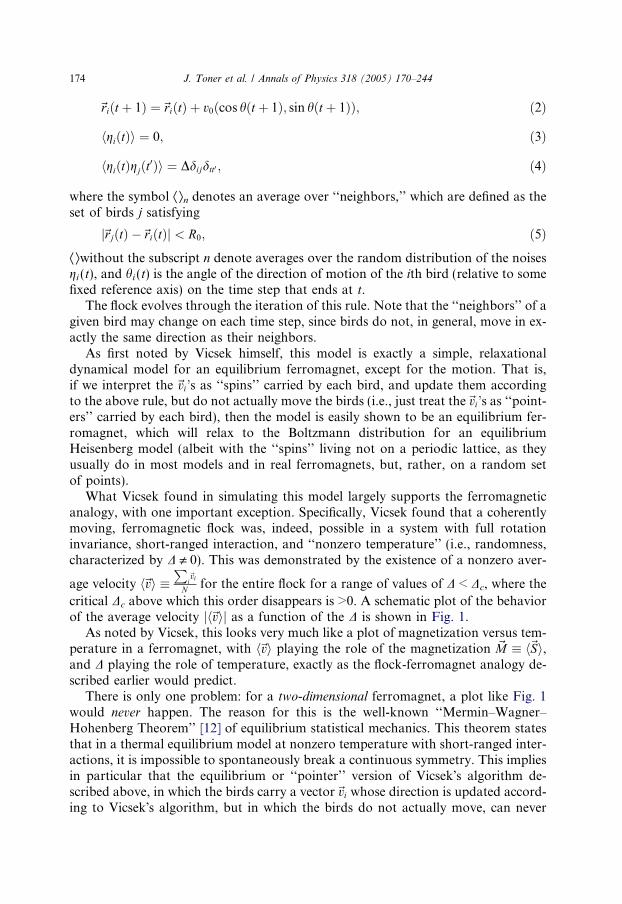
critical Dc above which this order disappears is >0. A schematic plot of the behaviorof the average velocity jh~vij as a function of the D is shown in Fig. 1.
As noted by Vicsek, this looks very much like a plot of magnetization versus tem-perature in a ferromagnet, with h~vi playing the role of the magnetization ~M � h~Si,and D playing the role of temperature, exactly as the flock-ferromagnet analogy de-scribed earlier would predict.
There is only one problem: for a two-dimensional ferromagnet, a plot like Fig. 1would never happen. The reason for this is the well-known ‘‘Mermin–Wagner–Hohenberg Theorem’’ [12] of equilibrium statistical mechanics. This theorem statesthat in a thermal equilibrium model at nonzero temperature with short-ranged inter-actions, it is impossible to spontaneously break a continuous symmetry. This impliesin particular that the equilibrium or ‘‘pointer’’ version of Vicsek�s algorithm de-scribed above, in which the birds carry a vector~vi whose direction is updated accord-ing to Vicsek�s algorithm, but in which the birds do not actually move, can never

Fig. 1. The magnitude of the average velocity jh~vij versus the noise strength D. The existence of the twophases, the moving (ordered) phase with jh~vij > 0 and the nonmoving (disordered) phase with jh~vij ¼ 0,are evident from the figure.
J. Toner et al. / Annals of Physics 318 (2005) 170–244 175
develop a true long-range ordered state in which all the~vi’s point, on average, in the
same direction (more precisely, in which h~vi �P
i~vi
N 6¼~0), since such a state breaks acontinuous symmetry, namely rotation invariance.
Yet the moving flock evidently has no difficulty in doing so; as Vicsek�s simulationshows, even two-dimensional flocks with rotationally invariant dynamics, short-ran-ged interactions, and noise—i.e., seemingly all of the ingredients of the Mermin–Wagner theorem—do move with a nonzero macroscopic velocity, which requiresh~vi 6¼~0, which, in turn, breaks rotation invariance, in seeming violation of the the-orem.
How can this be? Is the Mermin–Wagner theorem wrong? Are birds smarter than
nerds?The answer to the last two questions is, of course, no. The reason is that one of the
essential premises of the Mermin–Wagner theorem does not apply to flocks: they arenot systems in thermal equilibrium. The nonequilibrium aspect arises from the mo-tion of the birds.
Clearly, it must: as described above, the motion is the only difference between Vic-sek�s algorithm and a (slightly unconventional) equilibrium spin system. But how
does motion get around the Mermin–Wagner theorem? And, more generally, howbest to understand the large-scale, long-time dynamics of a very large, moving flock?
The answer to this second question can be found in the field of hydrodynamics.Hydrodynamics is a well-understood subject. This understanding does not come
from solving the many (very many!) body problem of computing the time-depen-dent positions ~riðtÞ of the 1023 constituent molecules of a fluid subject to intermo-lecular forces from all of the other 1023 molecules. Such an approach is analyticallyintractable even if one knew what the intermolecular forces were. Trying to

176 J. Toner et al. / Annals of Physics 318 (2005) 170–244
compute analytically the behavior of, e.g., Vicsek�s algorithm directly would be thecorresponding, and equally impossible, approach to the flocking problem.
Instead, the way we understand fluid mechanics is by writing down a set ofcontinuum equations—the Navier–Stokes equations—for a continuous, smoothlyvarying number density qð~r; tÞ and velocity~vð~r; tÞ fields describing the fluid.
Although we know that fluids are made out of atoms and molecules, we can define‘‘coarse-grained’’ number density qð~r; tÞ and velocity~vð~r; tÞ fields by averaging over‘‘coarse-graining’’ volumes large compared to the intermolecular or, in the flocks,‘‘interbird’’ spacing. On a large scale, even discrete systems look continuous, as weall know from close inspection of newspaper photographs and television images.
In writing down the Navier–Stokes equations, one ‘‘buries one�s ignorance’’ [13]of the detailed microscopic dynamics of the fluid in a few phenomenologicalparameters, namely the mean density q0, the bulk and shear viscosities gB andgS, the thermal conductivity j, the specific heat cv, and the compressibility v. Oncethese have been deduced from experiment (or, occasionally, and at the cost of im-mense effort, calculated from a microscopic model), one can then predict the out-comes of all experiments that probe length scales much greater than a spatialcoarse-graining scale ‘0 and timescales �t0, a corresponding microscopic time,by solving these continuum equations, a far simpler task than solving the micro-scopic dynamics.
But how do we write down these continuum equations? The answer to this ques-tion is, in a way, extremely simple: we write down every relevant term that is not ru-led out by the symmetries and conservation laws of the problem. In the case of theNavier–Stokes equations, the symmetries are rotational invariance, space and timetranslation invariance, and Galilean invariance (i.e., invariance under a boost to areference frame moving at a constant velocity), while the conservation laws are con-servation of particle number, momentum, and energy.
‘‘Relevant,’’ in this specification means terms that are important at large-lengthscales and long timescales. In practice, this means a ‘‘gradient expansion’’: we onlykeep in the equations of motion terms with the smallest possible number of spaceand time derivatives. For example, in the Navier–Stokes equations we keep a viscousterm gsr2~v, but not a term cr4~v, though the latter is also allowed by symmetry, be-cause the cr4~v term involves more spatial derivatives, and hence is smaller, for slowspatial variation, than the viscous term we have already got.
In Section 2, we will review the formulation and solution of such a hydrodynamicmodel for ‘‘ferromagnetic’’ flocks in [14–16].
In addition to these symmetries of the questions of motion, which reflect theunderlying symmetries of the physical situation under consideration, it is also neces-sary to treat correctly the symmetries of the state of the system under consideration.These may be different from those of the underlying system, precisely because thesystem may spontaneously break one or more of the underlying symmetries of theequations of motion. Indeed, this is precisely what happens in the ordered state ofa ferromagnet: the underlying rotation invariance of the system as a whole is brokenby the system in its steady state, in which a unique direction is picked out—namely,the direction of the spontaneous magnetization.

J. Toner et al. / Annals of Physics 318 (2005) 170–244 177
As should be apparent from our earlier discussion, this is also what happens in aspontaneously moving flock. Indeed, the symmetry that is broken—rotational—andthe manner in which it is broken—namely, the development of a nonzero expectationvalue for some vector (the spin ~S in the ferromagnetic case; the velocity h~vi in theflock) are precisely the same in both cases [7].
Many different ‘‘phases’’ [17], in this sense of the word, of a system with a givenunderlying symmetry are possible. Indeed, we have already described two suchphases of flocks: the ‘‘ferromagnetic’’ or moving flock, and the ‘‘disordered,’’ ‘‘para-magnetic,’’ or stationary flock.
In equilibrium statistical mechanics, this is precisely how we classify differentphases of matter: by the underlying symmetries that they break. Crystalline solids,for example, differ from fluids (liquid and gases) by breaking both translationaland orientational symmetry. Less familiar to those outside the discipline of softcondensed matter physics are the host of mesophases known as liquid crystals,in some of which (e.g., nematics [18]) only orientational symmetry is broken, whilein others, (e.g., smectics [18]) translational symmetry is only broken in some direc-tions, not all.
It seems clear that, at least in principle, every phase known in condensed mattersystems could also be found in flocks. To date, hydrodynamic models have been for-mulated for three such phases: the paramagnetic and ferromagnetic state [14–16,19,20] and the nematic [21] state. In intriguing contrast to the situation in thermalequilibrium systems, the long-wavelength stability of such phases is found to dependon the type of dynamics (momentum-conserving versus nonconserving, inertial ver-sus viscosity-dominated) obeyed by the system [19,21].
In particular, the theoretical work on the ferromagnetic state explains how suchsystems ‘‘get around’’ the Mermin–Wagner theorem, and exhibit long-ranged ordereven in d = 2.
In Section 5, we summarize the theoretical work on what we call ‘‘nematic’’ flocks,which are flocks in which the motion and/or orientation of the creatures picks out anaxis, but not a sense along that axis. This could happen (for example, but not exclu-sively) if the system settled down into a state in which creatures moved preferentiallyalong the x axis, say, half in the +x and half in the �x direction with the +x and �x
creatures well mixed. The state would then have zero mean velocity for the flock, butwould be uniaxially ordered. Nematic phases have been observed in, e.g., living mel-anocytes [9]. Dynamical states of exactly the same symmetry occur in agitated gran-ular materials composed of long, thin grains [22–24]. Surprisingly, even though suchflocks have no net motion, the continuum theory for this state, developed along thesame lines as that for the ferromagnetic state, predicts that their behavior is very dif-ferent from that of conventional equilibrium nematic liquid crystals, despite the factthat they have the same symmetry, just as ferromagnetic flocks are quite differentfrom their equilibrium counterparts.
In addition to changing which symmetries are broken (i.e., which phase we areconsidering) in a flock, we can also consider different underlying symmetries. Thesimplest such change of underlying symmetry is considered in Section 4, in whichwe treat ferromagnetic flocks which move in a non-rotationally invariant environ-

178 J. Toner et al. / Annals of Physics 318 (2005) 170–244
ment. Specifically, we consider ‘‘easy-plane’’ models, in which the ‘‘birds’’ prefer tofly in a particular plane (e.g., horizontally), which is obviously the case for many realexamples.
A more dramatic change is to restore Galilean invariance. The work on ferromag-netic and nematic flocks described above dealt with systems lacked this symmetry,which is usually included in fluid mechanics. To lack Galilean invariance simplymeans that the equations of motion do not remain the same in a moving coordinatesystem. This is appropriate if we are modeling creatures moving in the presence offriction over (or through) a static medium; e.g., wildebeest moving over the surfaceof the Serengeti plane, bacteria crawling over the surface of a Petri dish, etc. It isequally clearly not appropriate for creatures moving through a medium which is it-self fluid (e.g., the air birds fly through, the water fish swim through). In these cases,there is an additional symmetry (Galilean invariance) not present in the previousmodels, which leads to additional conservation laws (of total momentum of flockplus background fluid), which in turn lead to additional hydrodynamic variables(e.g., total momentum density), and a completely different hydrodynamic descrip-tion.
Hydrodynamic models of both ferromagnetic and nematic flocks movingthrough such a background fluid [19] are reviewed in Section 6, where it is shownthat nematic flocks in suspension have an inviscid instability at long wavelengths.The most striking prediction of this section, however, is that ‘‘ferromagnetic’’flocks in suspension are unstable at sufficiently low Reynolds number. This meansit is impossible in principle to find long-range ordered swimming bacteria; in theabsence of external aligning fields, a large flock of bacteria initially all swimmingin the same direction must break up into finite flocks with velocities uncorrelatedfrom flock to flock. The section also summarizes predictions [20] for novel rheo-logical properties of isotropic flocks as their correlation length and time are in-creased. Experimental evidence for the instability of ferromagnetic flocks insuspension is reviewed in Section 7, along with many other experiments doneon flocking.
In Section 8, we discuss a number of experiments we would like to see done. The-ory is currently far ahead of experiment in this field, an unhealthy situation that canbe corrected by careful measurements of fluctuations in flocks to test, quantitatively,the many detailed predictions that are available from the theories described in Sec-tions 2–5.
Finally, in Section 9, we discuss possible directions for future research in this area.We hope to make clear there that the subject of flocking is an extremely rich and fer-tile one, the surface of which we have scarcely scratched. In particular, as discussedearlier, virtually every one of the dozens of phases known in soft condensed matterphysics should have an analog in flocks. So far, as mentioned earlier, only three ofthese phases have even had their hydrodynamics formulated, and only two of them(the ordered ferromagnetic and nematic states) have really been investigated thor-oughly. The study of the rich variety of other possible phases of flocks therefore re-mains a wide open subject, potentially as intriguing as any in Condensed Matter ofPhysics, as well as being of obvious interest to anyone interested in biology, zoology,

J. Toner et al. / Annals of Physics 318 (2005) 170–244 179
and dynamical systems. We hope that this review will stimulate further research onthis rich, fascinating, and still largely unexplored subject.
The remainder of this paper is organized as follows: in Section 2, we review thehydrodynamic theory of ferromagnetic flocks in isotropic (i.e, fully rotationallyinvariant) environments. In Section 3, we describe numerical experiments confirmingthe theory in detail, and addressing the phase transitions in these systems as well. InSection 4, we consider ‘‘easy-plane’’ models, in which the ‘‘birds’’ prefer to fly in aparticular plane (e.g., horizontally), which is obviously the case of many real exam-ples. In these models, the positions of the birds are fully extended over 3 (or, as atheorist�s toy model, more) dimensions; it is just the velocities of the birds that liepreferentially in a plane (e.g., consider a tall, broad, and deep flock of flamingoes fly-ing horizontally). In Section 5, we discuss nematic flocking, while Section 6 treats theincorporation of ‘‘solvent hydrodynamic effects’’ (e.g., the motion of the backgroundfluid) on ferromagnetic, nematic, and disordered flocks. In Section 7, we discuss theexperimental work that has been done to date testing some of these ideas, while inSection 8 we provide a ‘‘wish-list’’ of experiments we would like to see done, whichwould provide detailed quantitative tests of the theories we describe here. This sec-tion will also lay out in detail precisely what those quantitative predictions are, andhow experiments can test them. Experimentalists interested in testing our ideasshould proceed directly to this section, which is fairly self-contained.
And finally, we conclude in Section 9 by suggesting several directions for futurework. Our list is necessarily abbreviated; any clever reader can no doubt think ofmany equally fascinating problems in this area which are not on our list, but shouldbe studied. This is a fascinating field with room for many more researchers, both the-oretical and experimental.
2. Isotropic ferromagnetic flocks
2.1. Formulating the hydrodynamic model
In this section, wewill review the derivation and analysis of the hydrodynamicmod-el of ferromagnetic flocks.Amore detailed discussion can be found in [16].As discussedin Section 1, the systemwewish tomodel is any collection of a large numberNof organ-isms (hereafter referred to as ‘‘birds’’) in a d-dimensional space, with each organismseeking to move in the same direction as its immediate neighbors.
We further assume that each organism has no ‘‘compass’’; in the sense defined inSection 1, i.e., no intrinsically preferred direction in which it wishes to move. Rather,it is equally happy to move in any direction picked by its neighbors. However, thenavigation of each organism is not perfect; it makes some errors in attempting to fol-low its neighbors. We consider the case in which these errors have zero mean; e.g., intwo dimensions, a given bird is no more likely to err to the right than to the left ofthe direction picked by its neighbors. We also assume that these errors have no longtemporal correlations; e.g., a bird that has erred to the right at time t is equally likelyto err either left or right at a time t 0 much later than t.

180 J. Toner et al. / Annals of Physics 318 (2005) 170–244
The continuum model will describe the long distance behavior of any flock satis-fying the symmetry conditions we shall specify in a moment. The automaton studiedby Vicsek et al. [5] described in Section 1 provides one concrete realization of such amodel. Adding ‘‘bells and whistles’’ to this model by, e.g., including purely attractiveor repulsive interactions between the birds, restricting their field of vision to thosebirds ahead of them, giving them some short-term memory, etc., will not changethe hydrodynamic model, but can be incorporated simply into a change of thenumerical values of a few phenomenological parameters in the model, in much thesame way that all simple fluids are described by the Navier–Stokes equations, andchanging fluids can be accounted for simply by changing, e.g., the viscosity that ap-pears in those equations.
This model should also describe real flocks of real living organisms, provided thatthe flocks are large enough, and that they have the same symmetries and conserva-tion laws that, e.g., Vicsek�s algorithm does.
So, given this lengthy preamble, what are the symmetries and conservation laws offlocks?
The only symmetries of the model are invariance under rotations and transla-tions. Translation-invariance simply means that displacing the positions of thewhole flock rigidly by a constant amount has no physical effect, since the spacethe flock moves through is assumed to be on average homogeneous [25]. Since weare not considering translational ordering, this symmetry remains unbroken andplays no interesting role in what follows, any more than it would in a fluid. Rotationinvariance simply says the ‘‘birds’’ lack a compass, so that all direction of space areequivalent to other directions. Thus, the ‘‘hydrodynamic’’ equation of motion wewrite down cannot have built into it any special direction picked ‘‘a priori’’; alldirections must be spontaneously picked out by the motion and spatial structureof the flock. As we shall see, this symmetry severely restricts the allowed terms inthe equation of motion.
Note that themodel does not haveGalilean invariance: changing the velocities of allthe birds by some constant boost~vb does not leave the model invariant. Indeed, such aboost is impossible in amodel that strictly obeysVicsek�s rules, since the speeds of all thebirds will not remain equal to v0 after the boost. One could image relaxing this con-straint on the speed, and allowing birds to occasionally speed up or slow down, whiletending an average to move at speed v0. Then the boost just described would be possi-ble, but clearly would change the subsequent evolution of the flock.
Another way to say this is that birds move through a resistive medium, which pro-vides a special Galilean reference frame, in which the dynamics are particularly sim-ple, and different from those in other reference frames. Since real organisms in flocksalways move through such a medium (birds through the air, fish through the sea, wil-debeest through the arid dust of the Serengeti), this is a very realistic feature of themodel [26].
As we shall see shortly, this lack of Galilean invariance allows terms in the hydro-dynamic equations of birds that are not present in, e.g., the Navier–Stokes equationsfor a simple fluid, which must be Galilean invariant, due to the absence of a luminif-erous ether.

J. Toner et al. / Annals of Physics 318 (2005) 170–244 181
The sole conservation law for flocks is conservation of birds: we do not allowbirds to be born or die ‘‘on the wing.’’
In contrast to the Navier–Stokes equation, there is no conservation of momentumin the models discussed in this section. This is, ultimately, a consequence of the ab-sence of Galilean invariance.
Having established the symmetries and conservation laws constraining our model,we need now to identify the hydrodynamic variables. They are precisely the same asthose of a simple fluid [27]: the coarse grained bird velocity field ~vð~r; tÞ, and thecoarse grained bird density qð~r; tÞ. The field~vð~r; tÞ, which is defined for all~r, is a suit-able weighted average of the velocities of the individual birds in some volume cen-tered on ~r. This volume is big enough to contain enough birds to make theaverage well-behaved, but should have a spatial linear extent of no more than afew ‘‘microscopic’’ lengths (i.e., the interbird distance, or by a few times the interac-tion range R0). By suitable weighting, we seek to make~vð~r; tÞ fairly smoothly varyingin space.
The density qð~r; tÞ is similarly defined, being just the number of particles in acoarse graining volume, divided by that volume.
The exact prescription for the coarse graining should be unimportant, so long asqð~r; tÞ is normalized so as to obey the ‘‘sum rule’’ that its integral over any macro-
scopic volume (i.e., any volume compared with the aforementioned microscopiclengths) be the total number of birds in that volume. Indeed, the coarse grainingdescription just outlined is the way that one imagines, in principle, going over froma description of a simple fluid in terms of equations of motion for the individual con-stituent molecules to the continuum description of the Navier–Stokes equation.
We will also follow the historical precedent of the Navier–Stokes [13,28] equationby deriving our continuum, long wavelength description of the flock not by explicitlycoarse graining the microscopic dynamics (a very difficult procedure in practice), but,rather, by writing down the most general continuum equations of motion for~v and qconsistent with the symmetries and conservation laws of the problem. This approachallows us to bury our ignorance in a few phenomenological parameters, (e.g., the vis-cosity in the Navier–Stokes equation) whose numerical values will depend on the de-tailed microscopic rules of individual bird motion. What terms can be present in theEOMs, however, should depend only on symmetries and conservation laws, and not
on other aspects of the microscopic rules.To reduce the complexity of our equations of motion still further, we will perform
a spatio-temporal gradient expansion, and keep only the lowest order terms in gra-dients and time derivatives of~v and q. This is motivated and justified by our desire toconsider only the long distance, long time properties of the flock. Higher order termsin the gradient expansion are ‘‘irrelevant’’: they can lead to finite ‘‘renormalization’’of the phenomenological parameters of the long wavelength theory, but cannot
change the type of scaling of the allowed terms.With this lengthy preamble in mind, we now write down the equations of motion:
ot~vþ k1ð~v � ~rÞ~vþ k2ð ~r �~vÞ~vþ k3 ~rðj~vj2Þ
¼ a~v� bj~vj2~v� ~rP þ DB~rð ~r �~vÞ þ DTr2~vþ D2ð~v � ~rÞ2~vþ~f ; ð6Þ

182 J. Toner et al. / Annals of Physics 318 (2005) 170–244
P ¼ P ðqÞ ¼X1n¼1
rnðq� q0Þn; ð7Þ
oqot
þr � ð~vqÞ ¼ 0; ð8Þ
where b, DB, D2, and DT are all positive, and a < 0 in the disordered phase and a > 0in the ordered state (in mean field theory). The origin of the various terms is as fol-lows: the k terms on the left-hand side of Eq. (6) are the analogs of the usual convec-tive derivative of the coarse-grained velocity field ~v in the Navier–Stokes equation.Here the absence of Galilean invariance allows all three combinations of one spatialgradient and two velocities that transform like vectors; if Galilean invariance did ap-ply here, it would force k2 = k3 = 0 and k1 = 1. However, as we have argued above,we are not constrained here by Galilean invariance, and so all three coefficients arenonzero phenomenological parameters whose nonuniversal values are determined bythe microscopic rules. The a and b terms simply make the local ~v have a nonzeromagnitude ð¼
ffiffiffiffiffiffiffiffia=b
pÞ in the ordered phase, where a > 0. DB,T,2 are the diffusion con-
stants (or viscosities) reflecting the tendency of a localized fluctuation in the veloci-ties to spread out because of the coupling between neighboring ‘‘birds.’’ Amusingly,it is these ‘‘viscous’’ terms that contain the ‘‘elasticity’’ of an ordered flock—therestoring torques that try to make parallel the orientation of neighboring birds.The ~f term is a random driving force representing the noise. We assume it is Gauss-ian with white noise correlations
hfið~r; tÞfjð~r 0; t0Þi ¼ Ddijddð~r �~r 0Þdðt � t0Þ; ð9Þ
where D is a constant, and i, j denote Cartesian components. Finally, P is the pres-sure, which tends to maintain the local number density qð~rÞ at its mean value q0, anddq = q � q0. Strictly speaking, here too, as in the case of the ‘‘viscous’’ terms involv-ing DB,T,2, we should distinguish gradients parallel and perpendicular to~v, i.e., gra-dients in the density should be allowed to have independent effects along andtransverse to ~v in (6). In an equilibrium fluid this could not happen, since Pascal�sLaw ensures that pressure is isotropic. In the nonequilibrium steady state of a flock,no such constraint applies. For simplicity, however, we ignore this possibility here,and consider purely longitudinal pressure forces.
The final Eq. (8) is just conservation of bird number (we do not allow our birds toreproduce or die on the wing).
Symmetry allows any of the phenomenological coefficients ki, a, rn, b, and Di inEqs. (6) and (7) to be functions of the squared magnitude j~vj2 of the velocity, and ofthe density q as well.
2.2. The broken symmetry ferromagnetic state
The hydrodynamic model embodied in Eqs. (6)–(8) is equally valid in both the ‘‘dis-ordered’’ (i.e., nonmoving) (a < 0) and ‘‘ferromagnetically ordered’’ (i.e., moving)(a < 0) state. In this section, we are mainly interested in the �ferromagnetically
J. Toner et al. / Annals of Physics 318 (2005) 170–244 183
ordered,’’ broken-symmetry phase; specifically in whether fluctuations around thesymmetry broken ground state destroy it (as in the analogous phase of the 2DXYmod-el). For a > 0, we can write the velocity field as~v ¼ v0xk þ ~dv, where v0xk ¼ h~vi is thespontaneous average value of~v in the ordered phase. We will chose v0 ¼
ffiffia
p
b (which
should be thought of as an implicit condition on v0, since a andb can, in general, dependon j~vj2); with this choice, the equation of motion for the fluctuation dvi of vi is
otdvk ¼ �r1okdq� 2advk þ irrelevant terms. ð10Þ
Note now that if we are interested in ‘‘hydrodynamic’’ modes, by which we meanmodes for which frequency x fi 0 as wave vector q fi 0, we can, in the hydrody-namic (x,q fi 0) limit, neglect otdvi relative to advi in (10). The resultant equationcan trivially be solved for dvi
dvk ¼ �ðr1=2aÞokdq. ð11Þ
Inserting (11) in the equations of motion for ~v? and dq, we obtain, neglecting‘‘irrelevant’’ terms:
ot~v? þ cok~v? þ k1 ~v? � ~r?
� �~v? þ k2 ~r? �~v?
� �~v?
¼ �~r?P þ DB~r? ~r? �~v?� �
þ DTr2?~v? þ Dko
2k~v? þ~f ?; ð12Þ
odqot
þ qo~r? �~v? þ ~r? � ð~v?dqÞ þ v0okdq ¼ Dqo
2jjdq; ð13Þ
where Dq � q0r12a, DB, DT, and Dk � DT þ D2v20 are the diffusion constants, and we
have defined
c � k1v0. ð14ÞThe pressure P continues to be given, as it always will, by Eq. (7).
From this point forward, we will treat the phenomenological parameters ki, c, andDi appearing in Eqs. (12) and (13) as constants, since they depend, in our originalmodel (6), only on the scalar quantities j~vj2 and qð~rÞ, whose fluctuations in the bro-ken symmetry state away from their mean values v20 and q0 are small. Furthermore,these fluctuations lead only to ‘‘irrelevant’’ terms in the equations of motion.
It should be emphasized here that, once nonlinear fluctuation effects are included,the v0 in Eq. (13) will not be given by the ‘‘mean’’ velocity of the birds, in the sense of
hvi �jPi~vij
N; ð15Þ
where N is the number of birds. This is because, in our continuum language
hvi ¼hRqð~r; tÞ~vð~r; tÞddri
�� ��hRqð~r; tÞddri
¼ hq~vij jhqi ð16Þ
while v0 in Eq. (14) is
v0 ¼ jh~vð~r; tÞij. ð17Þ

184 J. Toner et al. / Annals of Physics 318 (2005) 170–244
Once q fluctuates, so that q = Æqæ + dq, the ‘‘mean’’ velocity of the birds
hvi ¼ hq~vihqi
�������� ¼ hqih~vi
hqi þ hdq~vihqi
�������� ð18Þ
which equals v0 � jh~vij only if the correlation function hdq~vi ¼ 0, which it will not, ingeneral. For instance, one could easily imagine that denser regions of the flock mightmove faster; in which case hdq~vi would be positive along h~vi. Thus, h~vi measured in asimulation by simply averaging the speed of all birds, as in Eq. (15), will not be equalto v0 in Eq. (14). Indeed, we can think of no simple way to measure v0, and so choseinstead to think of it as an additional phenomenological parameter in the brokensymmetry state equations of motion (12) and (13). It should, in simulations andexperiments, be determined by fitting the correlation functions we will calculate inthe next section. One should not expect it to be given by Ævæ as defined in Eq. (16).
Similar considerations apply to c: it should also be thought of as an independent,phenomenological parameter, not necessarily determined by the mean velocity andnonlinear parameter k1 through (14).
2.3. Linearized theory of the broken symmetry ferromagnetic state
As a first step towards understanding the implications of these equations of mo-tion, we linearize them in~v? and dq ” q � q0. Doing this, and Fourier transformingin space and time, we obtain the linear equations:
�i x� cqk� �
þ CTð~qÞh i
~vTð~q;xÞ ¼ ~f Tð~q;xÞ; ð19Þ
�i x� cqk� �
þ CLð~qÞh i
vL þ ir1q?dq ¼ fLð~q;xÞ; ð20Þ
�i x� v0qk� �
þ Cqð~qÞh i
dqþ iq0q?vL ¼ 0; ð21Þ
where
vLð~q;xÞ �~q? �~v?ð~q;xÞ
q?ð22Þ
and
~vTð~q;xÞ ¼~v?ð~q;xÞ �~q?vLq?
ð23Þ
are the longitudinal and transverse (to~q?) pieces of the velocity,~f Tð~q;xÞ and fLð~q;xÞare the analogous pieces of the Fourier transformed random force~f ð~q;xÞ, andwe havedefined wavevector dependent transverse, longitudinal, and q dampings CL,T,q:
CLð~qÞ � DLq2? þ Dkq2k; ð24Þ
CTð~qÞ ¼ DTq2? þ Dkq2k; ð25Þ
Cqð~qÞ ¼ Dqq2k; ð26Þ
where we have defined DL ” DT + DB, q? ¼ j~q?j.
J. Toner et al. / Annals of Physics 318 (2005) 170–244 185
Note that in d = 2, the transverse velocity~vT does not exist: no vector can be per-pendicular to both the xi axis and ~q? in two dimensions. This leads to many impor-tant simplifications in d = 2, as we will see later; these simplifications make it (barely)possible to get exact exponents in d = 2 for the full, nonlinear problem.
It is now a straightforward exercise in linear algebra to solve these linearizedequations for the hydrodynamic mode structure of a flock. By ‘‘hydrodynamicmode-structure’’ we simply mean the eigenfrequencies xð~qÞ of the homogeneousequations obtained by setting the noise term ~f ¼~0. It is just as straightforward tosolve these linearized equations for ~vð~q;xÞ and qð~q;xÞ in terms of ~f ð~q;xÞ. Usingthe known correlations of ~f from Eq. (9) given earlier, one can thereby straightfor-wardly compute the correlations of ~vð~q;xÞ and qð~q;xÞ with each other, and withthemselves. Readers interested in the details of these calculations are referred to[16]; here we simply summarize the results.
The normal modes of these equations are d � 2 purely diffusive transverse modesassociated with~vT, all of which have the same eigenfrequency
xT ¼ cqk � iCTð~qÞ ¼ cqk � i DTq2? þ Dkq2k� �
ð27Þ
and a pair of damped, propagating sound modes with complex (in both senses of theword) eigenfrequencies
x� ¼ c�ðh~qÞq� iCL
v�ðh~qÞ2c2ðh~qÞ
� �� iCq
v�ðh~qÞ2c2ðh~qÞ
� �
¼ c�ðh~qÞq� iðDLq2k þ D?q2?Þv�ðh~qÞ2c2ðh~qÞ
� �� iDqq2k
v�ðh~qÞ2c2ðh~qÞ
� �; ð28Þ
where h~q is the angle between ~q and the direction of flock motion (i.e., the xi axis):
c�ðh~qÞ �cþ v02
cosðh~qÞ � c2ðh~qÞ; ð29Þ
v�ðh~qÞ � � c� v02
cosðh~qÞ þ c2ðh~qÞ; ð30Þ
c2ðh~qÞ �ffiffiffiffiffiffiffiffiffiffiffiffiffiffiffiffiffiffiffiffiffiffiffiffiffiffiffiffiffiffiffiffiffiffiffiffiffiffiffiffiffiffiffiffiffiffiffiffiffiffiffiffiffiffiffiffiffiffiffiffiffiffiffi1
4ðc� v0Þ2cos2ðh~qÞ þ c20sin
2ðh~qÞr
; ð31Þ
and c0 �ffiffiffiffiffiffiffiffiffir1q0
p. A polar plot of this highly anisotropic sound speed is given in
Fig. 2.We remind the reader that here and hereafter, we only keep the leading order
terms in the long wave length limit, i.e., for small qi and q^.These direction-dependent sound speeds can most easily be determined experi-
mentally by measuring the spatio-temporally Fourier-transformed density–densitycorrelation function Cqqð~q;xÞ � hjqð~q;xÞj2i. We will describe in detail in Section 7how to easily obtain this correlation function from observation of a flock via, e.g.,computer imaging of a film. The linearized calculation described above predicts thatthis density–density correlation function, when considered as a function of frequencyx, has two sharp peaks at x ¼ c�ðh~qÞq, with widths of O(q2), as illustrated in Fig. 3.
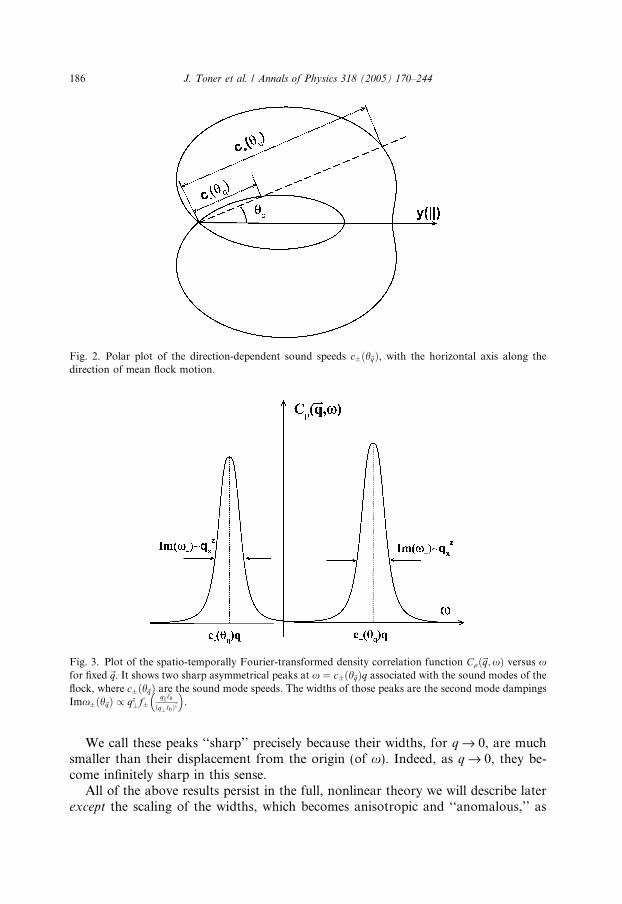
Fig. 2. Polar plot of the direction-dependent sound speeds c�ðh~qÞ, with the horizontal axis along thedirection of mean flock motion.
Fig. 3. Plot of the spatio-temporally Fourier-transformed density correlation function Cqð~q;xÞ versus xfor fixed~q. It shows two sharp asymmetrical peaks at x ¼ c�ðh~qÞq associated with the sound modes of theflock, where c�ðh~qÞ are the sound mode speeds. The widths of those peaks are the second mode dampingsImx�ðh~qÞ / qz?f�
qk‘0
ðq?‘0Þf
� �.
186 J. Toner et al. / Annals of Physics 318 (2005) 170–244
We call these peaks ‘‘sharp’’ precisely because their widths, for q fi 0, are muchsmaller than their displacement from the origin (of x). Indeed, as q fi 0, they be-come infinitely sharp in this sense.
All of the above results persist in the full, nonlinear theory we will describe laterexcept the scaling of the widths, which becomes anisotropic and ‘‘anomalous,’’ as

J. Toner et al. / Annals of Physics 318 (2005) 170–244 187
will be described in Section 2.4. The peaks do remain sharp, however, and their posi-tions are correctly predicted by the linearized theory.
The exact expression for Cqqð~q;xÞ that we obtain is
Cqq ¼Dq2
0q2?
ðx� cþðh~qÞqÞ2ðx� c�ðh~qÞqÞ2 þ ðxðCLð~qÞ þ Cqð~qÞÞ � qkðv0CLð~qÞ þ cCqð~qÞÞÞ2.
ð32Þ
We can similarly find the velocity autocorrelations
Cijð~q;xÞ � hv?i ð�~q;�xÞv?j ð~q;xÞi � CTTð~q;xÞP?ij ð~qÞ þ CLLð~q;xÞL?
ij ð~qÞ; ð33Þ
where:
L?ij ð~qÞ �
q?i q?j
q2?; ð34Þ
P?ij ð~qÞ � d?ij � L?
ij ð~qÞ; ð35Þ
are longitudinal and transverse projection operators in the plane perpendicular tothe mean flock motion
CTTð~q;xÞ ¼D
ðx� cqkÞ2 þ C2
Tð~qÞð36Þ
and
CLLð~q;xÞ¼Dððx� v0qkÞ
2þC2qð~qÞÞ
ðx� cþðh~qÞqÞ2ðx� c�ðh~qÞqÞ2þðxðCLð~qÞþCqð~qÞÞ�qkðv0CLð~qÞþ cCqð~qÞÞÞ2.
ð37Þ
The transverse and longitudinal correlation functions in Eqs. (36) and (37) are plot-ted as functions of x for fixed ~q in Fig. 4.
Note that they have weight in entirely different regions of frequency: CTT ispeaked at x = cqi, while CLL, like Cqq, has two peaks, at x ¼ c�ðh~qÞq. Since all threepeaks have widths of order q2, there is little overlap between the transverse and thelongitudinal peaks as j~qj ! 0.
With the velocity correlations Cijð~q;xÞ in hand, we can now address the questionwhich first caught our attention: Are birds smarter than nerds? That is, do flocksobey the Mermin–Wagner theorem?
To answer this, we need to calculate the real-space, real-time fluctuationshj~vð~r; tÞj2i.
To have true long-ranged orientational order, which is necessary to have an or-dered, coherently moving flock, these fluctuations must remain finite as the size ofthe flock goes to infinity. To calculate hj~vð~r; tÞj2i from Cijð~q;xÞ, we must FourierTransform back to real space ~r and real time t from ~q and x space, respectively.Going back to real time first gives the spatially Fourier transformed equal timevelocity correlation function:
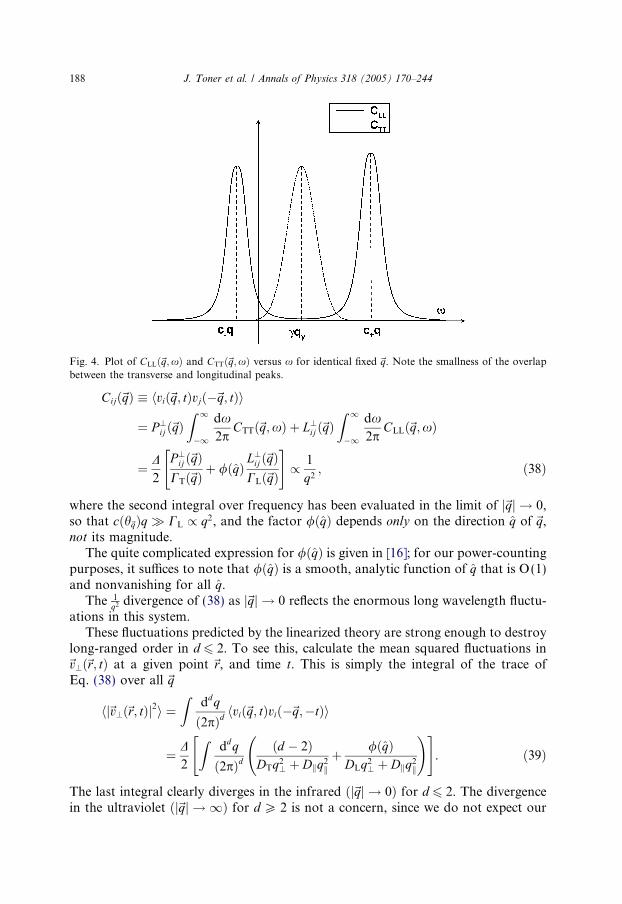
Fig. 4. Plot of CLLð~q;xÞ and CTTð~q;xÞ versus x for identical fixed ~q. Note the smallness of the overlapbetween the transverse and longitudinal peaks.
188 J. Toner et al. / Annals of Physics 318 (2005) 170–244
Cijð~qÞ � hvið~q; tÞvjð�~q; tÞi
¼ P?ij ð~qÞ
Z 1
�1
dx2p
CTTð~q;xÞ þ L?ij ð~qÞ
Z 1
�1
dx2p
CLLð~q;xÞ
¼ D2
P?ij ð~qÞ
CTð~qÞþ /ðqÞ
L?ij ð~qÞ
CLð~qÞ
" #/ 1
q2; ð38Þ
where the second integral over frequency has been evaluated in the limit of j~qj ! 0,so that cðh~qÞq � CL / q2, and the factor /ðqÞ depends only on the direction q of ~q,not its magnitude.
The quite complicated expression for /ðqÞ is given in [16]; for our power-countingpurposes, it suffices to note that /ðqÞ is a smooth, analytic function of q that is O(1)and nonvanishing for all q.
The 1q2 divergence of (38) as j~qj ! 0 reflects the enormous long wavelength fluctu-
ations in this system.These fluctuations predicted by the linearized theory are strong enough to destroy
long-ranged order in d 6 2. To see this, calculate the mean squared fluctuations in~v?ð~r; tÞ at a given point ~r, and time t. This is simply the integral of the trace ofEq. (38) over all ~q
hj~v?ð~r; tÞj2i ¼Z
ddq
ð2pÞdhvið~q; tÞvið�~q;�tÞi
¼ D2
Zddq
ð2pÞdðd � 2Þ
DTq2? þ Dkq2kþ /ðqÞDLq2? þ Dkq2k
!" #. ð39Þ
The last integral clearly diverges in the infrared ðj~qj ! 0Þ for d 6 2. The divergencein the ultraviolet ðj~qj ! 1Þ for d P 2 is not a concern, since we do not expect our

J. Toner et al. / Annals of Physics 318 (2005) 170–244 189
theory to apply for j~qj larger than the inverse of a microscopic length (such as theinteraction range ‘0).
The infra-reddivergence inEq. (39) for d 6 2 cannot be dismissed so easily, since ourhydrodynamic theory should get better as j~qj ! 0. Indeed, in the absence of nonlineareffects, this divergence is real, and signifies the destruction of long-ranged order in thelinearized model by fluctuations, even for arbitrarily small noise D, in spatial dimen-sions d 6 2, and in particular in d = 2, where the integral in Eq. (39) diverges logarith-mically in the infra-red. This is so since, if hj~v?j2i is arbitrarily large even for arbitrarilysmall D, our original assumption that~v can be written as a mean value h~vi plus a small
fluctuation~v? is clearlymistaken; indeed, the divergence of~v? suggests that the velocitycan swing through all possible directions, implying that h~vi ¼ 0 for d 6 2.
In d = 2, this result is very reminiscent of the familiar Mermin–Wagner–Hohen-berg (MWH) theorem[12], which states that in equilibrium, a spontaneously brokencontinuous symmetry is impossible in d = 2 spatial dimensions, precisely because ofthe type of logarithmic divergence of fluctuations that we have just found here. In-deed, to the linear order we ave worked here, this model looks just like an equilib-rium model. All of the crucial differences between the equilibrium model and ourflocking model must therefore lie in the nonlinearities. In the next section, we willshow this is indeed the case: much of the scaling of correlation functions and prop-agators is changed from that predicted by the linearized theory in spatial dimensionsd 6 4. Most dramatically, this change in scaling makes it possible for flocks to devel-op long-ranged order even in d = 2, even though equilibrium systems cannot.
2.4. Non-linear effects and breakdown of linear hydrodynamics in the broken symmetry
state
2.4.1. Scaling analysis
In this section, we analyze the effect of the nonlinearities in Eqs. (12) and (13) onthe long length and time behavior of the system, for spatial dimensions d < 4. We willrescale lengths, time, and the fields~v? and dq according to:
~x? ! b~x?;
xk ! bfxk;
t ! bzt;
~v? ! bv~v?;
dq ! bvqdq.
ð40Þ
We begin by constructing the scaling which preserves the structure of the linearized
theory, and then see if the nonlinearities grow or shrink under this rescaling. Accord-ingly, we first choose the scaling exponents to keep the diffusion constants DB,T,q,i,and the strength D of the noise fixed. The reason for choosing to keep these partic-ular parameters fixed rather than, e.g., r1, is that these parameters completely deter-mine the size of the equal time fluctuations in the linearized theory, as can be seenfrom Eq. (39). Under the rescalings (40), the diffusion constants rescale accordingto DB,T fi bz�2DB,T and Dq,i fi bz�2fDq,i; hence, to keep them fixed, we must choose

190 J. Toner et al. / Annals of Physics 318 (2005) 170–244
z = 2 and f = 1. The rescaling of the random force ~f can then be obtained from theform of the f � f correlations Eq. (9) and is, for this choice of z and f
~f ! b�1�d=2~f . ð41ÞTo maintain the balance between ~f and the linear terms in~v? in Eq. (12), we mustchoose
v ¼ 1� d=2 ð42Þin Eq. (40). v is the roughness exponent for the linearized model, i.e., we expect~v?fluctuations on length scale L to scale like Lv. Therefore, the linearized hydrody-namic equations, neglecting the nonlinear convective terms and the nonlinearitiesin the pressure, imply that~v? fluctuations grow without bound (like Lv) as L fi 1for d 6 2, where the above expression for v becomes positive. Thus, this linearizedtheory predicts the loss of long range order in d 6 2, as we saw in the last sectionby explicitly evaluating the real space fluctuations.
Making the rescalings as described in Eq. (40), the equation of motion (12)becomes
ot~v? þ bcvcok~v? þ bck ½k1ð~v? � ~r?Þ~v? þ k2ð~r? �~v?Þ~v?�
¼ �~r?X1n¼1
bcnrnðdqÞn !
þ DB~r?ð~r? �~v?Þ þ DTr2
?~v? þ Djjo2jj~v? þ~f ? ð43Þ
with:
ck ¼ vþ 1 ¼ 2� d=2; ð44Þ
cv ¼ z� f ¼ 1; ð45Þand
cn ¼ z� vþ nv� 1 ¼ nþ ð1� nÞ d2. ð46Þ
The scaling exponent vq for dq is given by vq = v, since the density fluctuations dqare comparable in magnitude to the~v? fluctuations. To see this, note that the eigen-mode of the linearized equations of motion that involves dq is a sound mode, withdispersion relation x ¼ c�ðh~qÞq. Inserting this into the Fourier transform of the con-tinuity Eq. (13), we see that dq ~q?�~v?
q?. The magnitude of ~q? drops out of the right
hand side of this expression; hence dq scales like j~v?j at long distances. Therefore,we will choose vq ¼ v ¼ 1� d
2.
The first two of these scaling exponents for the nonlinearities to become positiveas the spatial dimension d is decreased are ck and c2, which both become positive ford < 4, indicating that the k1ð~v? � ~rÞ~v?; k2ð~r? �~v?Þ~v? and r2
~r?ðdq2Þ nonlinearitiesare all relevant perturbations for d < 4. So, for d < 4, the linearized hydrodynamicswill break down.
A very similar breakdown of linearized hydrodynamics has long been known [28]to occur in simple equilibrium fluids for d 6 2. Somewhat less well-known is themore dramatic, and experimentally verified, breakdown of linearized hydrodynamicsthat occurs in equilibrium smectic [29] and columnar [30] liquid crystals.

J. Toner et al. / Annals of Physics 318 (2005) 170–244 191
What can we say about the behavior of Eqs. (12) and (13) for d < 4, when the lin-earized hydrodynamics no longer holds? The answer is provided by the dynamicalrenormalization group, whose results we summarize in the next two sections. Thefirst of these presents the general form of the results in arbitrary spatial dimensionsd with 2 6 d 6 4, while the second presents results in d = 2 exactly, in which case wecan obtain exact exponents.
2.4.2. Renormalization group analysis, d < 4
In this section, we summarize the results of the dynamical renormalization groupanalysis of the effect of the nonlinearities in the flock equations of motion. Readersinterested in the details of the analysis (which are quite involved) are referred to [16].
The simplest summary of the scaling of all correlation functions and propagatorsis: simply use the harmonic expressions for them, except that the diffusion constantsDT,B,q should be replaced by wavevector-dependent quantities that diverge as~q ! 0,according to the scaling laws
DT ;B;qð~qÞ ¼ qz�2? fT;B;q
qkK
� �q?K
� �f !
; ð47Þ
the bare noise strength D should be replaced by
Dð~qÞ ¼ Dq?K
� �z�f�2vþ1�dfD
ðqkKÞðq?K Þf
!ð48Þ
and the diffusion constant Di should be replaced by
Dkð~qÞ ¼ qz�2f? fk
ðqkKÞðq?K Þf
!. ð49Þ
The scaling functions fD,B,T,q,i (u) in these expressions have the following asymp-totic limits:
fT;B;qðuÞ /constant; u ! 0;
uz�2f ; u ! 1;
(ð50Þ
fDðuÞ /constant; u ! 0;
uz�f�2vþ1�d
f ; u ! 1;
(ð51Þ
and
fkðuÞ /constant; u ! 0;
uzf�2; u ! 1.
ð52Þ
HereK 1/‘NL is an ultraviolet cutoff, with ‘NL the length scale at which nonlineareffects become important. a one-loop RG analysis predicts: lNL ð10D5=4
? D1=4jj =
kD1=2Þð2=ð4�dÞÞ �Oð1Þ. Higher loop corrections may affect this result, but it presumablyremains accurate to factors of O(1).
192 J. Toner et al. / Annals of Physics 318 (2005) 170–244
The form of these scaling functions is such that the renormalized diffusion con-stants and the noise strength depend only on qi for
qjjK � ðq?K Þ
f, and only on q^ inthe opposite limit. That is:
DT;B;qð~qÞ /qz�2? ;
qjjK � ðq?K Þf;
qz�2f
k ;qjjK � ðq?K Þf;
8<: ð53Þ
Dð~qÞ /qz�f�2vþ1�d? ;
qjjK � ðq?K Þf;
qz�f�2vþ1�d
f
k ;qjjK � ðq?K Þf;
8<: ð54Þ
and
Dkð~qÞ /qz�2f? ;
qjjK � ðq?K Þf;
qzf�2
k ;qjjK � ðq?K Þf.
8<: ð55Þ
None of the other parameters of the linearized theory is appreciably affected by thenonlinearities (beyond finite renormalizations). In particular, the sound speedsremain given by Eq. (29), with all of the parameters in that equation remainingconstants as q fi 0.
The divergence of these diffusion ‘‘constants’’ and noise correlations as q fi 0 isthe ‘‘breakdown of linearized hydrodynamics’’ that we argued in the last sectionwould occur below d = 4.
The physics of this breakdown is very simple: above d = 4, where the breakdowndoes not occur, information about what is going on in one part of the flock can betransmitted to another part of the flock only by being passed sequentially throughthe intervening neighbors via the assumed short-ranged interactions. Below d = 4,where the breakdown occurs, this slow, diffusive transport of information is replacedby direct, convective transport: fluctuations in the local velocity of the flock becomeso large, in these lower dimensions, that the motion of one part of the flock relativeto another becomes the principal means of information transport, because it be-comes faster than diffusion. There is a sort of ‘‘negative feedback,’’ in that this im-proved transport actually suppresses the very fluctuations that give rise to it [31],leading to long-ranged order in d = 2, as we will see in the next section.
The dynamical exponent z, the roughness exponent v, and the anisotropy expo-nent f completely characterize the scaling of the dynamics of flocks. Unfortunately,we have been unable to calculate them in any dimension except d = 2. All we know is6/5 < z < 2, v < min(�1/5,1 � d/2), and 3/5 < f < 1 for 2 < d < 4.
The origin of our uncertainty is the k2 term in Eq. (12). When k2 = 0, the structureof the theory is such that we can determine the exponents v, z, and f exactly. (Detailsof the somewhat involved argument are given in [16]; here we will simply sketch thereasoning.) This is because, when k2 = 0, all of the relevant pieces of the remainingvertices are total ^ derivatives. It is straightforward to show that an immediate con-sequence of this is that D and Di,q acquire no graphical renormalization when k2 = 0.The requirement that D, Di, and Dq flow to fixed points ðdDk;q
d‘Þ ¼ 0 ¼ dD
d‘leads to two
J. Toner et al. / Annals of Physics 318 (2005) 170–244 193
independent exact scaling relations between the three independent exponents v, z,and f. Requiring
dDk;qd‘
¼ 0 implies
z ¼ 2f ð56Þwhile requiring dD
d‘¼ 0 leads to
z ¼ fþ 2vþ d � 1. ð57ÞWe emphasize that we have only shown that these relations (56) and (57) hold whenk2 = 0.
We can obtain a third independent exact scaling relation between these threeexponents, and thereby determine them exactly, when k2 = 0, by exploiting a ‘‘pseu-do-Galilean’’ invariance that the equations of motion (12) and (13) have whenk1 = kq, which leads to a exact scaling relation, namely
v ¼ 1� z. ð58ÞThe three relations ((56)–(58) that hold when k2 = 0 can trivially be solved, to findthe exact scaling exponents in all d < 4 that describe flocks with k2 = 0:
f ¼ d þ 1
5; ð59Þ
z ¼ 2ðd þ 1Þ5
; ð60Þ
and
v ¼ 3� 2d5
. ð61Þ
Note that these match continuously, at the upper critical dimension d = 4, onto theirharmonic values f = 1, z = 2, and v ¼ 1� d
2¼ �1, as they should.
But can k2 be ignored? Only if it renormalizes to zero. We have performed adynamical RG analysis of this question, and find that k2 is unrenormalized at oneloop order, leading to an apparent fixed line at that order. Since we do not knowwhat happens to k2 at higher order, all we can say at this point is that there are threepossibilities:
1. At higher order, k2 renormalizes to zero. If this is the case, then Eq. (59)–(61) holdexactly, for all flocks, for d in the range 2 6 d 6 4. Note that these results linearlyinterpolate between the equilibrium results z = 2, f = 1, and v ¼ 1� d
2in d = 4,
and our 2d results z = 6/5, f = 3/5, and v = �1/5 in d = 2.2. At higher order, k2 grows upon renormalization and reaches a nonzero fixed point
value k2 at some new fixed point that differs from the k2 = 0 fixed point we havestudied previously, at which Eqs. (59)–(61) holds. The exponents v, z, and f wouldstill be universal (i.e., depend only on the dimension of space d) for all flocks inthis case, but those universal values would be different from Eqs. (59)–(61).
3. k2 is unrenormalized to all orders. Should this happen, k2 would parameterize afixed line, with continuously varying values of the exponents z, v, and f.

194 J. Toner et al. / Annals of Physics 318 (2005) 170–244
We reiterate: we do not know which of the above possibilities holds for d > 2.However, whichever holds is universal; that is, only one of the three possibilitiesabove applies to all flocks. We do not, however, know which one that is.
In any case, the exponents z, v, and f completely characterize the scaling of thedynamics and fluctuations in flocks for all dimensions d in the range 2 6 d 6 4. Thiscan be seen by looking at any of the quantities we calculated in our linearized treat-ment in Section 2.3. For example, the full dispersion relation for the sound modes is
x� ¼ c�ðh~qÞq� iqz?f�
qkK
ðq?K Þf
!; ð62Þ
which follows from Eq. (28) upon replacing the diffusion constants with their wave-vector-dependent values in Eqs. (47) and (49). The scaling function f± in this expres-sion obeys
f�ðuÞ /constant; u ! 0;
uz=f; u ! 1.
ð63Þ
As a result, the attenuation of sound scales like qz? forqjjK � ðq?K Þf, and like qz=fjj for
qjjK � ðq?K Þf.
As discussed in Section 2.3, the dispersion relations for x± and xs can be directlyprobed by measuring the spatio-temporally Fourier transformed density–density andvelocity–velocity auto-correlation functions Cqqð~q;xÞ and Cijð~q;xÞ.
These take exactly the same form as predicted in Section 2.3, with the replacementof the diffusion constants Dq,B,T with the wavevector-dependent quantities given inEqs. (47) and (49).
As a result, the two sharp peaks in Cqq at x = c± ðh~qÞq, now have width
/ qz?fLðqkK
ðq?K ÞfÞ and height / q�ð2vþzþ3fþd�3Þ? gð
qkK
ðq?K ÞfÞ, rather than the q2 and q�4 scaling
predicted by the linearized theory. Thus, c�ðh~qÞ can be simply extracted from the po-sition of the peaks, while the exponents v, z, and f can be determined by comparingtheir widths and heights for different ~q’s.
Fourier transformingCijð~q;xÞ back to real time gives an equation of the same formas (38), but with CL;Tð~qÞ and D modified from their linearized forms by the samereplacement of D�s and D by their renormalized, wavevector-dependent values Eqs.((47)–(49). This implies that the equal-time velocity correlationCijð~qÞ obeys the scalinglaws:
Cijð~qÞ /qz�f�2vþ1�d? ;
qjjK � ðq?K Þf;
qz�f�2vþ1�d
f
k ;qjjK � ðq?K Þf.
8<: ð64Þ
Since z < 2 and f < 1, these results imply that, for all d < 4, equal-time velocityfluctuations diverge more slowly than 1
q2 (the latter being both the equilibrium resultand that obtained by the linearized theory).
This suppression of fluctuations in Fourier space leads to fluctuations in real
space that are finite, even in d = 2, as we will show in detail in the next section.Specifically

J. Toner et al. / Annals of Physics 318 (2005) 170–244 195
hj~v?ð~r; tÞj2i ¼Z
ddq
ð2pÞdhvið~q; tÞvið�~q; tÞi
¼ 1
2
Zddq
ð2pÞdDð~qÞ ðd � 2Þ
DTð~qÞq2? þ Dkð~qÞq2kþ /ðqÞDLð~qÞq2? þ Dkð~qÞq2k
" #ð65Þ
remains finite, even in d = 2.So far, our discussion has focussed on velocity fluctuations. The density qð~r; tÞ
shows huge fluctuations as well: indeed, at long wavelengths, the fluctuations ofthe density of birds in a flock become infinitely bigger than those in a fluid or an idealgas. This fact is obvious to the eye in a picture of a flock. Quantitatively, Fouriertransforming Cqqð~q;xÞ back to real time yields the spatially Fourier transformed,equal time density–density correlation function Cqqð~qÞ � hjqð~q; tÞj2i, which obeysthe scaling law:
Cqqð~qÞ ¼q3�d�f�2v?q2
fq
qkK
ðq?K Þf
!Y ðh~qÞ /
q1�d�f�2v? ; qk � q?;
q�2jj q3�d�f�2v
? ; q?K
� �f � qkK � q?
K ;
q�3þ1�d�2v
f
k q2?; ðq?K Þf � qkK ;
8>>><>>>:
ð66Þwhere Y ðh~qÞ is a finite, nonvanishing, O(1) function of the angle h~q between thewavevector~q and the direction of mean flock motion, qi and~q? are the wavevectorsparallel and perpendicular to the broken symmetry direction, and q? ¼ j~q?j.
The most important thing to note about Cqð~qÞ is that it diverges as j~qj ! 0, unlikeCqð~qÞ for, say, a simple fluid or gas, or, indeed, for any equilibrium condensed mattersystem, which goes to a finite constant (the compressibility) as j~qj ! 0.
This completes our discussion of the behavior of the full, nonlinear model indimensions d between 2 and 4. We now turn to the behavior of the model in
d = 2, where we can actually determine the exponents exactly.
2.4.3. Ferromagnetic flock exponents in d = 2
In the last section, we argued that the three exponents z, v, and f which completelydetermine the scaling properties of the flock can be determined exactly if only onecould show that k2 fi 0 upon renormalization.
However, in d = 2, any flock is equivalent to a flock with k2 = 0. This is becausethe k1 and k2 vertices become identical in d = 2, where~v? has only one component,which we will take to be x. That is, in d = 2:
k1ð~v? � ~r?Þ~v? ¼ k1xvxoxvx ¼1
2k1oxðv2xÞx; ð67Þ
k2ð~r? �~v?Þ~v? ¼ k2xðoxvxÞvx ¼1
2k2oxðv2xÞx; ð68Þ
so that the full ~v? nonlinearity becomes 12ðk1 þ k2Þoxðv2xÞx, which is just what
we would get if we started with a (primed) model with k02 ¼ 0 and k01 ¼ k1 þ k2. This

196 J. Toner et al. / Annals of Physics 318 (2005) 170–244
latter model, since it has k02 ¼ 0, must have the ‘‘canonical’’ exponents (59)–(61)hence, so must the (k1,k2) model, which includes all possible d = 2 models. So allmodels in d = 2 must have the canonical exponents (59)–(61).
Setting d = 2 in (59)–(61), we obtain:
f ¼ 3
5; ð69Þ
z ¼ 6
5; ð70Þ
v ¼ � 1
5. ð71Þ
Note, in particular, that v < 0. This implies, as discussed earlier, that the flock exhib-its true long-ranged order.
Using the exponents (69)–(71) in the general scaling relations, such as (64) and(66), we obtain all of the scaling results for correlation functions in d = 2. Note alsothat for this set of exponents z � f � 2v + 1 � d = 0. Hence, from Eq. (48), we seethat the noise strength D is a constant, independent of ~q, which makes sense sinceD is unrenormalized graphically. So, in the d = 2 model, we can calculate all corre-lation functions from their harmonic expressions, except that we replace the diffusionconstants DB,T with functions that diverge as ~q ! 0 according to the scaling laws
DB;Tð~qÞ ¼ q�4=5? fB;T
qkK
� �q?K
� �3=5 !
; ð72Þ
where we have used the exact d = 2 exponents z = 6/5 and f = 3/5 in the generalscaling law (47). Di,q, on the other hand, are, like D, constants, since z = 2f (see gen-eral Eq. (49)), which also makes sense since Di,q are unrenormalized graphically.Hence, the only replacement needed to turn the harmonic results into the correctresults for the full, nonlinear theory in d = 2 is (72). Therefore, in d = 2, f = 3/5,and v = �1/5
Cqqð~qÞ ¼q4=5?q2
fqqk
K q?K
� �3=5 !
Y ðh~qÞ /
q�6=5? ; qk � q?;
q�2jj q
4=5? ; q?
K
� �3=5 � qkK � q?
K ;
q�4k q2?; ðq?K Þ3=5 � qk
K .
8>><>>: ð73Þ
These scaling predictions agree extremely well with numerical simulations [15,16],as we will discuss in detail in the next section.
3. Comparison with numerical simulations
Many aspects of flocking dynamics are too complex to be tractable analytically.Numerical simulation thus becomes an important and necessary tool in exploringthe rich phenomena in various flocking models. Even though the concept of simulat-

J. Toner et al. / Annals of Physics 318 (2005) 170–244 197
ing collective behaviors in self propelled systems was introduced to the physics com-munity by Vicsek et al. [5], computer models for flocks, not surprisingly, were usedearlier in disciplines as diverse as ecology and computer graphics[1], albeit with dif-ferent emphasis in each field. The main focus of the physicists in this field has beenthe (bulk) properties of the system in the limit of large system size, corresponding towhat we refer to, at thermal equilibrium, as the thermodynamic limit. We shall usethat term here as well, although we do not mean to suggest that the properties of thatlimit for equilibrium systems, such as equivalence of ensembles, hold here as well.We would like to understand the types of possible nonequilibrium steady states,i.e., phases of the system, and the nature of the changes from one type of phase toanother when parameters are changed, i.e., the nature of the nonequilibrium phasetransitions. In this section, we review numerical simulation studies in this area, withdiscussions of their connections to both the analytical results and the actual exper-imental observations, whenever possible.
3.1. Possible behaviors (phases)
The Vicsek model does not include any interaction to enforce a preferred distancebetween boids, which are kept together only by the periodic boundary conditions inthe Vicsek�s original study[5]. While the Vicsek model probably yields an adequatedescription of the transition from the moving to the nonmoving state in large sys-tems, it cannot capture the behavior of finite flocks and of possible positional, as dis-tinct from orientational order within the flock.
Following a model introduced by biologists Huth and Wissel [1] in the early 1990sfor describing real bird flocks, the Vicsek model can be generalized by adding a cen-tral force between each pair of boids within a distance R of each other. Since themain function of such interaction is to keep the flock together, it can be called the‘‘cohesive interaction.’’ At each time step, a total force vector is determined by sum-ming the cohesive interaction, the velocity alignment interaction and a random noise[32] for each boid i
~f i ¼Xj
ðafaðrijÞ~vj þ bfbðrijÞrijÞ þ~gi; ð74Þ
where j represents all the neighbors [33] within a radius R centered around the ithboid, ~vj is the velocity of j, and rij is the unit vector from i to j. a and b are thestrengths of the aligning and cohesive forces, respectively, and the distance-depen-dence is contained in the functions fa,b (rij), where rij is the distance between boidsi and j. ~gi is a noise with unit amplitude and random angle. At the next time step,the velocity of boid i changes its direction to that of ~f i, and the boid i moves withthat velocity to its new position. After each boid�s position and velocity have beenupdated, the process is repeated with the new position and velocity of the boids.
In two separate papers [34,35], the general qualitative behaviors of the flockingmodel with cohesive force were examined with specific choices of the interactionfunctions fa,b (rij). In [35], the strength of the alignment force is set to be constantfa (rij) = 1 and the form of the cohesive force was taken to be

Fig. 5. Sketch of the asymptotic phase diagram in the zero-density limit. Due to the large separation ofscales in b, the phase diagram is broken into two panels to show details of the transition regions. Filledcircles indicate points determined numerically in [35] for a system of size L = 180, q = 1/16, see text for theparameters of the model.
198 J. Toner et al. / Annals of Physics 318 (2005) 170–244
fbðrijÞ ¼�1 : rij < rc;14
rij�rera�re
: rc < rij < ra;
1 : ra < rij < R.
8><>:
With the parameters rc = 0.2, ra = 0.8, re = 0.5, R = 1.0, and v0 = 0.05 fixed, variousbehaviors of the flock were then studied in the parameter space spanned by the rel-ative strength (with respect to noise) of the cohesive (b) and the alignment (a) forcesin [35]. Fig. 5 summarizes the different behaviors of the system in the zero-densitylimit.
There are five different kinds of behaviors, which can be loosely called as ‘‘phas-es’’: moving solid (MS), stationary solid (S), moving liquid (ML), stationary liquid(L), and the gas phase (G). For small values of b, the boids do not stay togetheras a single group; instead they form smaller clusters or fly solo. We call this regionthe gas phase. The rest of the parameter space where the boids stay in one cluster ispartitioned into four phases. In general, as a increases, the flock starts to move, andas b increases, the boids seems to transform from the liquid phase, where their rel-ative positions are constantly changing, to the solid phase, where the relative posi-tions are fixed. In Fig. 6, the structures of these four condensed phases for a smallsystem are shown, each with several snap shots in time, to illustrate the differentflocking behaviors.
The moving and nonmoving phases can be distinguished by the average velocityof the system, as in [5]. To distinguish between the solid and the liquid phases, a rel-ative diffusion constant D over some large time T of initially neighboring boids wasused in [35]
D � 1
ni
Xji
1� rijðtÞ2
r2ijðt þ T Þ
!* +i;t
; ð75Þ

Fig. 6. Structures of condensed phases for a small system of 128 particles, and L = 32. (A) Immobile‘‘solid’’ at a = 1.0 and b = 100.0 (20 timesteps superimposed). (B)‘‘Flying crystal’’ at a = 3.0 and b = 100.0(three snapshots, separated by 120 timesteps). (C) Stationary fluid droplet at a = 1.0 and b = 2.0 (20consecutive timesteps). (D) Moving droplet at a = 3.0 and b = 3.0 (20 consecutive timesteps). (B and D)The arrow indicates the (instantaneous) direction of motion.
J. Toner et al. / Annals of Physics 318 (2005) 170–244 199
where ni is the number of neighbors (in the Voronoi sense) for the ith boid at time t.Time T was taken to be proportional to the volume of the system, which ensures thatD records, in the large-size limit, an asymptotic property of the system. D measuresthe inter-boid mixing inside the flock. Clearly, D 1 in the liquid phases, while D 0for the solid phases. For finite system sizes, the transition point was chosen to be atD ¼ 1
2.
It is clear that the flocking model exhibits much richer behaviors once the cohesiveforce is taken into account. The topology of the phase diagram is generally in agree-ment with our intuition and it is also evident from Fig. 5 that there are strong inter-actions between the two orders (positional and orientational) as reflected by thecurvatures of the phase boundaries. However, to establish the existence of thesephases in the thermodynamic sense requires much larger flocks and longer runningtime. In particular, as we see from the next section, the nature of the phase transitionis very subtle, and extremely large simulation size is needed to understand it.

200 J. Toner et al. / Annals of Physics 318 (2005) 170–244
3.2. The nature of the order to disorder transition
As described before, the global orientational order of the system is described bythe average velocity of all the boids in the system. By changing the noise strengthor the size of the system with constant number of boids, Vicsek et al. [5,36] foundthat the order parameter decreased to zero at a critical point continuously, suggest-ing a second order or, more generally, continuous, phase transition between a or-dered and a disordered phase for the system. By doing a finite scaling analysis, aset of critical exponents were also obtained to characterize the critical point [36].
However, in a recent numerical study with much larger system size by Gregoireand Chate [37], the continuous nature of the moving to nonmoving phase transitionwas challenged. Gregoire and Chate showed strong evidence for a discontinuoustransition between the ordered and disordered phases of the Vicsek model. The re-sults of their simulation are summarized in Fig. 7. From their simulation of large sys-tems, the disordered phase can be best described as many finite clusters of boids,
Fig. 7. Discontinuous character of the onset of collective motion in the original Vicsek model at q = 1/8.(A) The Binder cumulant G ” 1 � Æ/4æ/3Æ/2æ2 versus noise g at various system sizes. (B) Density (bottomcurve) and velocity (top curve) profiles along the direction of motion in the ordered phase (L = 1024,g = 0.18). (C) PDF of the instantaneous order parameter /t near the transition point, t 2 [s,500s]; s . 105
is the correlation (persistent) time, L = 512. (D) Snapshot of coarse-grained density field in disorderedphase at the threshold, q = 2, L = 256. The arrows indicate the direction of motion of dense, orderedclusters.

J. Toner et al. / Annals of Physics 318 (2005) 170–244 201
each moving in a different direction, coexisting with a dilute background of statisti-cally stationary boids (Fig. 7D). Each finite ordered cluster evolves in time by collect-ing and losing boids from the background, they can also nucleate from and dissolveinto the background. The ordered phase, on the other hand, consists of one or a fewlarge clusters of boids with some intriguing internal density and velocity profile (Fig.7B). Gregoire and Chate argued that because these two distinctive states coexist (atleast near the transition point) for finite system size, these two states occur alter-nately in time, leading to a seemingly continuous order parameter variation, whichis probably what was observed in Vicsek�s original numerical simulations. As the sys-tem size increases, the persistence time for each state becomes longer and, in the ther-modynamic limit, the transition becomes discontinuous.
Perhaps the strongest evidence for a discontinuous transition is provided by thebimodal distribution of the coarse-grained local order parameter observed nearthe transition point, as shown in Figs. 7A and C. Similar characteristics of the orderparameter were also found in other variations of the Vicsek model including oneswith different forms of the noise, thus substantiating the claim of a discontinuoustransition. Could the discontinuous nature of the transition be a special feature ofthe Vicesk model due to its lack of cohesive force? To answer this question, Gregoireand Chate [37] also investigated the moving to nonmoving transition for flockingmodels with cohesive interaction in large systems. Near the critical point in the dis-ordered phase, they found the disordered phase again consists of many small clustersconnected by thin filaments of boids, each small cluster moving in different directionsin much the same way as in the original Vicsek model. Gregoire and Chate thereforeargued that the transition between the ordered state and this ‘‘near critical’’ disor-dered state resembled the order to disordered transition in the Vicsek model, andthe onset to collective motion is always discontinuous even in the presence of cohe-sive force.
At the phenomenological level, it is evident that the nature of the transition is gov-erned by the strong interaction between the positional and the orientational degreesof freedom of the system. One possibility is that the transition from the (velocity) ori-entationally ordered phase to the disordered phase may be caused by a finite wave-length instability for the density profile. Such instability could break the extendedlarge cluster into many finite size ones, each of which moves in a different direction,leading to the vanishing of the global order parameter. At the theoretical level, it re-mains a challenge to formulate the proper interaction between density fluctuationand the directional order parameter near the ordering transition, which could thenbe used to understand the nature of the transition analytically.
3.3. The properties of the ordered phase
Away from the transition point into the ordered phase, things are a little clearer.Theoretically, the ordered phase (with uniform density) is found to be stable againstfluctuations caused by the spontaneous (orientational) symmetry breaking [14–16].However, despite its simple average behavior, the stable ordered phase has highlynontrivial properties in terms of its positional and orientational fluctuations due

202 J. Toner et al. / Annals of Physics 318 (2005) 170–244
to the interaction between the sound wave and the (soft) Goldstone mode. Some ofthe characteristics of these fluctuations, especially those in two dimensions, can bedetermined from the analytical analysis of the coarse grained continuum equations.In this section, we review the work done by Tu et al. [15] where the properties of boththe density and velocity fluctuations in the ordered phase were studied numericallyand compared directly with the predictions from the analytical work based on thecontinuum equations.
The model used in [15] is similar to the modified Vicsek model given in Eq. (74).At a given time t, the position and the direction of the velocity for each boid are gi-ven as ð~riðtÞ; hiðtÞÞ for i = 1,2, . . . ,N. The magnitude of the velocity is fixed: j~vij ¼ v0,its direction is updated at the next time step by averaging over its neighbors� movingdirections
hiðt þ 1Þ ¼ H1
M
XMj¼1
ð~vjðtÞ þ~gijðtÞÞ þ ~giðtÞ !
; ð76Þ
where M is the number of neighbors for boid i within radius R: rij ¼ j~ri �~rjj < R.The extra interaction term ~gij ¼ g0ð~ri �~rjÞððl0rij Þ
3 � ðl0rij Þ2Þ makes boids repel each
other when they are closer than l0, and attract each other otherwise, with l0 the aver-age distance between boids in the flock. In [15], a high boid density q : ql20 1 waschosen to prevent the formation of clusters, which render the average density profilenonuniform and complicate the analysis. The noise term ~giðtÞ ¼ DvðcosðpeiðtÞÞ;sinðpeiðtÞÞÞ, where ei (t) is a random number in the interval [�1,1]. The functionHð~xÞ is just the polar angle of the vector ~x. The position update is simply:~riðt þ 1Þ ¼~riðtÞ þ v0ðcosðhiðtÞÞ; sinðhiðtÞÞÞ. The parameters in this model are R, l0,Dv, v0, and g0.
The particular form of the interactions should not affect the universal predictionsof the continuum theory presented above, but rather should only change nonuniver-sal phenomenological parameters like c, k, Di, etc. They also affect the length scalelNL beyond which the asymptotic long wavelength forms of the correlation functions(32) and (37) apply. Indeed, a one-loop RG analysis predicts: lNL ð10ðDo
?Þ5=4
ðDojjÞ
1=4=koD
1=2o Þð2=ð4�dÞÞ �Oð1Þ, where the sub-(or super-)script o denotes the ‘‘bare,’’
or unrenormalized, value of the corresponding parameter. Higher loop correctionsmay affect this result, but it presumably remains accurate to factors of O(1).
For the current numerical model, the parameters for the corresponding contin-uum equations can be estimated on dimensional grounds: ko 1, Do ðDvÞ2 Rd
t0,
Dojj Do
? R2
t0. Inserting these estimates, one finds lNL Rð10RDvt0
Þð2=4�dÞ. In the simula-tion carried out in [15], choosing units of length and time such that R = t0 = 1, andtaking Dv Dvc 1/3 in these units, for d = 2 a lower bound for lNL: lNL > 30 wasobtained. Previous simulations [36] took Dv � 1, and therefore have a much largerlNL. Hence, no nontrivial nonlinear effects could be observed since their systems weremuch smaller than lNL.
The above analysis shows that in order to test the scaling behavior with a reason-able system size, one seeks a small lNL by increasing Dv and decreasing the radius ofinteraction R as much as possible without entering the disordered phase. In the study

Fig. 8. (A) The order parameter /, as defined in the text, versus the noise strength Dv. The arrow showsthe value of Dv at which the fluctuations of the ordered state were calculated. (B) The scaling behavior ofthe equal time correlation function for the density fluctuations in the two limits can be calculatedanalytically (see [14,15] for details) in two dimensions. The lines illustrate the predicted slopes.
J. Toner et al. / Annals of Physics 318 (2005) 170–244 203
by Tu et al. [15], the results of a simulation with system size L · L with L = 400 andthe number of boids N = 320,000 were reported. For the parameter values R = 1,g0 = 0.6, v0 = 1.0, l0 = .707 used in [15], the flock becomes disordered at Dvc .375(see Fig. 8A). The order parameter / is defined simply as the magnitude of the aver-age velocity of the whole flock: / ¼ 1
NjPN
i¼1~vij. To stay in the ordered phase and haveenough fluctuations, a large but subcritical value of noise Dv = 0.15 was chosen in[15].
For any finite flock, the direction of the average velocity will slowly change, ren-dering difficult any comparison to the analytical results, which assume infinite systemsize and hence a constant direction for h~vi. To make h~vi constant in its direction,periodic boundary conditions in one of the directions, say the x direction, andreflecting boundary conditions in the other direction y were used in [15]. When aboid i with velocity ðvxi ; v
yi Þ collides with the ‘‘walls’’ at y = ± L/2, its velocity changes
to ðvxi ;�vyi Þ. The symmetry broken velocity is thus forced to lie along the x-direction,without changing the bulk dynamics of the system. Hereafter ‘‘i’’ and x are usedinterchangeably, as are ‘‘^’’ and y.
The equal time correlation functions can be derived analytically from the contin-uum model, as shown in Eq. (73), from which we see that there are three regimes of~qspace with different scalings of Cqqð~qÞ with~q. In Fig. 8B, the equal time density cor-relation functions are plotted in Fourier space: Cqq (qi, q^ = 2p/L) versus qi andCqq (qi = 0,q^) versus q^ from our simulation. The scaling behavior at long lengthscales can be fitted with: Cqqðqjj; q? ¼ 2p=LÞ q�2.05
jj and Cqqðqjj ¼ 0; q?Þ q�1.23? .
These two exponents show excellent agreement with the analytical results �2 and�6/5 predicted in Eq. (73), once one recognizes that all of the ~q’s in the first fit liein the region ðq?K Þ3=5 � qk
K � q?K , where the analytical model predicts scaling as q�2
k .As can be seen from Fig. 8B, the scaling region for the current simulation coversslightly less than one decade in q^. It is not surprising that earlier simulations ofsmaller systems with less carefully chosen parameters (leading to larger lNL), didnot observe the nontrivial scaling.

204 J. Toner et al. / Annals of Physics 318 (2005) 170–244
Another interesting measurement of the simulation is the anomalous diffusion ofindividual boids in the direction y perpendicular to the flock�s moving direction. The‘‘width’’ of the dispersion of an ensemble of boids: w2 (t) = Æ(yi (t) � yi(0))
2æ was mea-sured in the simulation. The analytical behavior of the anomalous diffusion can beobtained from w2ðtÞ
R t0
R t0hviyðt0Þviyðt00Þidt0 dt00, where viyðtÞ is the velocity of the ith
boid along y direction at time t. The velocity correlation function is given by (4):
hviyð0ÞviyðtÞi hvyð~xþ /xt; tÞvyð~x; 0Þi
¼Z
expðiðx� /qjjÞtÞDðx� vsqjjÞ2 d2qdx
Sð~q;xÞ t1�1=f ð77Þ
which implies: w2ðtÞ t3�1=f ¼ t4=3. In Fig. 9, the width squared w2 (t) versus time t
from the numerical model was plotted in log–log scale. The scaling can be fitted ni-cely with w2 (t) t1.3, which agrees well with the analytical result t4=3.
Besides the scaling behavior, the analytical results (32), (37) also imply the exis-tence of sound waves as reflected in the peaks of the correlation functions Eqs.(32) and (37). From Eq. (32), at a given value of~q, the correlation function has peaksat x = c±(hq) q. This prediction is tested by measuring the power spectrum in the y-direction: hjdqðqjj ¼ 0; q? ¼ 2p
L n?;x ¼ 2pT nxÞj2i (T = 1024) with different values of
n^(= 1,2, . . . , 20). Fig. 10 shows the power spectra for n^ = 5, 10, 20. The spectraare symmetric around x = 0 (only half of the spectrum for x > 0 is shown) andthe positions of the peaks nx versus ny are shown in the inset of Fig. 10, whose slopedetermines the sound velocity in the y-direction c = 0.62. The power spectrum of v^in the y direction was calculated also, which shows the same peaks.
Along the x direction, i.e., with qi „ 0 and q^ = 0, the analytical study predicts onesingle peak for each correlation function. Indeed, as shown in figure Fig. 11, eachpower spectrum shows only one peak, and again as predicted by (32), (37), the peakfor the v^ power spectrum is at a different x than the peak of the density power spec-
Fig. 9. The log–log plot of the anomalous transverse diffusion of an individual boid versus time.

Fig. 10. The power spectrum of the density for different wave vectors. The inset shows the peak positionsof the power spectrum versus wavenumber. The linear slope determines the sound velocity.
Fig. 11. Power spectra for the density and velocity fluctuations for the same wave vector along the paralleldirection. The peaks of the two curves are clearly different.
J. Toner et al. / Annals of Physics 318 (2005) 170–244 205
trum! This means that the velocity fluctuations propagate with a different velocitythan the density fluctuations in the x-direction!
The comparison between the numerical model and the analytical equations can bemade at the quantitative level even beyond the values of exponents. From Fig. 12,the values of vs and k for the continuum model can be determined from the simula-

Fig. 12. The power spectra for the density and the velocity fluctuations in directions (A) hq,1 = arctan(4)and (B) hq,2 = arctan(1/3). The two peaks are clearly visible, albeit with different magnitudes. (C) Thewave velocities c±(hq) are plotted in polar angle coordinates (c±(hq),hq) for the four different directionshq = 0, hq,1, hq,2, p/2, the two axes represent cx = c±(hq) cos(hq) and cy = c±(hq) sin(hq), respectively. Thesolid curve is the prediction from the continuum model.
206 J. Toner et al. / Annals of Physics 318 (2005) 170–244
tion: vs = 0.93, k = 0.75. (The fact that k „ 1 reflects the absence of Galilean invari-ance.) With the value of c = 0.62 determined through Fig. 12, the sound speeds in allother directions of propagation can be predicted from Eq. (29) with no adjustableparameters. To test these predictions, the power spectra for the density and thevelocity fields were calculated in the numerical model at two other angles:tan(hq) = 1/3, 4. For the large angle hq,1 = arctan (4) = 76.0�, the data are shownin Fig. 12A. The peaks for q and v^ are at the same location, and the wave velocitiesare c±(hq,1) = 0.75, �0.37. The data for hq,2 = arctan(1/3) = 18.4 � are shown in Fig.12B. The peak at x = c� (hq,2) is just barely visible in the density correlation, butboth peaks show very well in the velocity correlation, and the peaks for both corre-lation functions are at the same locations, giving the velocity c±(hq,2) = 0.97, 0.59. InFig. 12C, the full angle dependence of the wave velocity as predicted in Eq. (29) inpolar angle coordinates (c±(hq), hq) is plotted, with the values of vs, k, and c deter-mined earlier. Included in Fig. 12C are also the sound velocities for the two angleshq,1 and hq,2 measured in the numerical model. The agreement with the predictedvelocities is excellent.

J. Toner et al. / Annals of Physics 318 (2005) 170–244 207
In summary, the numerical simulations strongly support the analytical continuumtheory of flocks. The observed sound speeds agree very well with predictions fromthe analytical model based on continuum equations of motion. In particular, theanalytical model�s assertion that Galilean invariance is absent is confirmed by theexistence of two different nonzero sound speeds for propagation along the meandirection of flock motion. In addition, the sound attenuation shows the anomalousscaling predicted analytically.
However, all the results presented here are based on the premise that the orderedstate has a homogeneous density profile, which was enforced in the numerical studyin [15] by having a boid density q compatible with the preferred inter-boid distance.If the ordered state has an inhomogeneous density profile, as reported in [37] for theVicsek model with low boid density, the nature of the density and velocity fluctuationcould be different, depending on the detailed structure of the average boid density pro-file.
4. Anisotropic model
Not all flocks, of course, are equally likely to move in any direction in the spacethey occupy. Flocks of birds, for instance, although they occupy a d = 3-dimensionalvolume (the air), are far more likely to move horizontally than vertically. This is pre-sumably because gravity breaks the rotational symmetry between the horizontalplane and vertical directions.
One can imagine a variety of ‘‘microscopic’’ rules, like the Vicsek rule described ear-lier, that would exhibit such anisotropy. For example, one could apply a ‘‘Vicsek’’ rulein three dimensions, selecting thereby a vector n. Instead of moving along that vector,however, one could instead move along a vector ‘‘compressed’’ along some (z) axis
~n0 ¼ snzzþ~n? ð78Þwith s < 1 and~n? ¼ n� nzz. This will tend to promote motion in the x–y plane at theexpense of motion in the z-direction. Alternatively, one could project all velocitiesinto the x–y plane, apply a Vicsek rule to them (while still sampling neighbors inthree dimensions), and then add to this xy move a random decorrelated step inthe z direction [38].
In this section, we will review the work of [16] on such anisotropic models.For technical reasons that will, we hope, become obvious, we will focus our atten-
tion on systems which, whatever their spatial dimension d, have an easy plane of mo-tion; i.e., two components of velocity that are intrinsically favored over the otherd � 2. We will also assume perfect isotropy within this plane and within the d � 2dimensional ‘‘hard’’ subspace. The case of birds flying horizontally corresponds tod = 3.
A natural extension of our fully isotropic model (EOM) to this case is
ot~vþ k1ð~v � ~rÞ~vþ k2ð~r �~vÞ~vþ k3~rðj~vj2Þ
¼ �~rP ðqÞ þ a~v� b~vj j2~v� da~vH þ DB~rð~r �~vÞ þ De
Tr2e~vþ DH
Tr2H~v
~ 2 ~
þ D2ð~v � rÞ ~vþ f . ð79Þ
208 J. Toner et al. / Annals of Physics 318 (2005) 170–244
Mass conservation, of course, still applies
otqþ ~r � ðq~vÞ ¼ 0 ð80Þand the pressure P (q) will still be given by the same expansion in dq = q � qo
P ðqÞ ¼X1n¼1
rnðdqÞn. ð81Þ
In Eq. (79),~vH denotes the d � 2 ‘‘hard’’ components of~v, i.e., those orthogonal tothe d = 2 easy plane. Likewise, r2
e and r2H denote the operators
P2i¼1
o2
ox2iandPd
i¼3o2
ox2i, respectively, where i = 1, 2 are the ‘‘easy’’ Cartesian directions, and
i = 3 fi d the ‘‘hard’’ ones. The term �daj~vHj2, da > 0 suppresses these componentsrelative to those in the easy plane.
Eq. (79) is not, of course, the most general anisotropic model we could writedown. For instance, one could have anisotropy in the nonlinear terms: e.g, terms likeð~ve � ~rÞ~ve could have different coefficients than ð~vH � ~rÞ~vH. However, because ~vHwinds up being ‘‘massive,’’ in the sense of decaying to zero too rapidly (i.e., nonhy-drodynamically) at long wavelengths and times to nonlinearly affect the hydrody-namic (long wavelength, long time) behavior of the flock (in its low temperaturephase), any additional terms in (79) distinguishing ~vH and~ve will have no effect onthe hydrodynamic behavior in the low ‘‘temperature’’ phase. That is, (79) alreadycontains enough anisotropy to generate all possible relevant, symmetry allowedterms in the broken symmetry state. Hence, we will keep things simple and not gen-eralize (79) further.
As we did for the isotropic problem, we will now break the symmetry of this mod-el, i.e., look for solutions to the form
~vð~r; tÞ ¼ h~vi þ d~vð~r; tÞ. ð82ÞNow, however, the direction of the mean velocity h~vi (which we will chose as be-
fore, to be a static, spatially uniform solution of the noiseless ð~f ¼ 0Þ version of (79))is not arbitrary, but must lie in the easy (1,2) plane. To see this, let us, without loss ofgenerality, write
h~vi ¼ voy y þ vozz ð83Þwith voy and voz constants, y in the easy plane and z one of the d � 2 ‘‘hard’’ direc-tions. To solve (79) with ~f ¼ 0, these must obey
avoy � bðv2oy þ v2ozÞvoy ¼ 0 ð84Þ
and
ða� daÞvoz � bðv2oy þ v2ozÞvoz ¼ 0 ð85Þ
Subtracting voy· (85) from voz ·; (84) we obtain davoyvoz = 0, which implies thateither voy or voz must be zero. It is straightforward to show that the former solutionis unstable (with two linear eigenvalues a > 0) to small~ve fluctuations, while the latteris stable (with d � 2 linear eigenvalues �da > 0) to ~vH fluctuations, so the solutionwith h~vi in the easy plane is the stable one. Furthermore, fluctuations in the ‘‘hard’’
J. Toner et al. / Annals of Physics 318 (2005) 170–244 209
directions are ‘‘massive,’’ in the sense of decaying rapidly to zero even at long wave-lengths, and so can be neglected in the low temperature phase (just like vi fluctua-tions in the isotropic case). Likewise, if we take
h~vi ¼ voy ð86Þfluctuations in dvy = vy � vo, will also be massive (with linear eigenvalue—2a). Elim-inating the massive fields dvy and~vH in favor of the pressure, as we did for dvi in theisotropic case, gives:
dvy ¼ �Dqyoyq; ð87Þ
~vH ¼ �DqH~rHq; ð88Þ
where we have defined the diffusion constants:
Dqy �r1
2a; ð89Þ
DqH � r1
da; ð90Þ
and we have used the relation (81) for the pressure, and dropped all but the leadingorder linear terms in dq, since higher powers of d q in Eqs. (87) and (88) prove to beirrelevant.
Using the solutions (87) and (88), and taking, for the reasons just discussed
~vð~rÞ ¼ ðvo þ dvyð~r; tÞÞy þ vxð~r; tÞxþ~vHð~r; tÞ ð91Þwe can write a closed system of equations for vxð~r; tÞ and dqð~r; tÞ:
otdqþ vooydqþ oxðqvxÞ ¼ ðDqyo2y þ DqHr2
HÞdq; ð92Þ
otvx þ coyvx þk2oxðv2xÞ ¼ �r1oxðdqÞ � r2oxðdqÞ2 þ ðDko
2y þDxo
2x þDHr2
HÞvx þ fx;
ð93Þwhere we have defined k ” k1 + k2, and c = k1v0, and dropped irrelevant terms.
Proceeding as we did in the isotropic model, we begin by linearizing these equa-tions, Fourier transforming them, and determining their mode structure.
The result of the first two steps is the Fourier transformed equations of motion:
½�iðx� voqyÞ þ Cqð~qÞ�dqð~q;xÞ þ iqxq0vxð~q;xÞ ¼ 0; ð94Þ
½�iðx� cqyÞ þ Cvð~qÞ�vxð~q;xÞ þ ir1qxdqð~q;xÞ ¼ fxð~q;xÞ; ð95Þ
where we have defined:
Cqð~qÞ � Dqyq2y þ DqHq2H; ð96Þ
Cvð~qÞ � Dkq2y þ DHq2H þ Dxq2x . ð97Þ
Again as in the isotropic model, we first determine the eigenfrequencies xð~qÞ ofthese equations, finding

210 J. Toner et al. / Annals of Physics 318 (2005) 170–244
x�ð~qÞ ¼ c� h~q;/~q
� �q� i��ð~qÞ; ð98Þ
where the sound speeds
c�ðh~q;/~qÞ ¼1
2ðcþ v0Þ cos h~q � c2ðh~q;/~qÞ ð99Þ
with
c2ðh~q;/~qÞ �ffiffiffiffiffiffiffiffiffiffiffiffiffiffiffiffiffiffiffiffiffiffiffiffiffiffiffiffiffiffiffiffiffiffiffiffiffiffiffiffiffiffiffiffiffiffiffiffiffiffiffiffiffiffiffiffiffiffiffiffiffiffiffiffiffiffiffiffiffiffiffiffiffiffi1
4ðc� v0Þ2cos2h~q þ r1q0sin
2h~qcos2/~q
r; ð100Þ
where h~q is the polar angle between ~q and the y-axis, and /~q is the azimuthal angle,measured relative to the x-axis: i.e., the angle between the projection of~q orthogonalto y, and the x-axis.
A polar plot of this sound speed versus h~q for /~q ¼ 0 (i.e.,~q in the ‘‘easy’’ (i.e., x–y) plane) looks exactly like that for the isotropic model (Fig. 2). Indeed, any slicewith fixed /~q looks qualitatively like that figure, although, as /~q ! p
2(i.e., as ~q?,
the projection of ~q orthogonal to y, approaches orthogonality to the x-axis), thesound velocity profile becomes two circles with their centers on the y axis and bothcircles passing through the origin.
The dampings ��ð~qÞ in (98) are 0 (q2), and given by
��ð~qÞ ¼ �c�ðh~q;/~qÞ2c2ðh~q;/~qÞ
ðCvð~qÞ þ Cqð~qÞÞ �v0 cosðh~qÞ2c2 h~q;/~q
� � Cvð~qÞ þcv0Cqð~qÞ
�. ð101Þ
Note that, unlike the isotropic problem in d > 2, here there are no transversemodes in any d: we always have just two longitudinal Goldstone modes associatedwith dq and vx.
We can now again parallel our treatment of the isotropic model and calculate thecorrelation functions and propagators. The calculation is so similar that we will notrepeat the details, but merely quote the results:
Cvvð~q;xÞ ¼D½ðx� voqyÞ
2 þ C2qð~qÞ�
jDen ~q;xð Þj2; ð102Þ
Cqvð~q;xÞ ¼ hdqð~q;xÞvxð�~q;�xÞi ¼Dr1qxðx� voqy � iCqð~qÞÞ
jDenð~q;xÞj2; ð103Þ
and
Cqqð~q;xÞ ¼Dq2
0q2x
jDenð~q;xÞj2; ð104Þ
where we have defined
Denð~q;xÞ ¼ ðx� cþðh~q;/~qÞqÞðx� c�ðh~q;/~qÞqÞ þ i½xðCqð~qÞ þ Cvð~qÞÞ� qyðvoCvð~qÞ þ cCqð~qÞÞ� ð105Þ
which, of course, implies

J. Toner et al. / Annals of Physics 318 (2005) 170–244 211
jDenð~q;xÞj2 ¼ ðx� cþðh~q;/~qÞqÞ2ðx� c�ðh~q;/~qÞqÞ
2 þ ½xðCqð~qÞ
þ Cvð~qÞÞ � qyðvoCvð~qÞ þ cCqð~qÞÞ�2. ð106Þ
These horrific expressions actually look quite simple when plotted as a function of xat fixed ~q; indeed, such a plot of Cvv looks precisely like Fig. 3: two asymmetricalpeaks, centered at x ¼ c�ðh~q;/~qÞq, with widths ��ð~qÞ / q2.
Note that, at this linear order, everything scales as it did in the isotropic problem:peak positions �q, widths �q2, and heights / 1
q4.Continuing to blindly follow the path we trod for the isotropic problem, we can
calculate the equal-time vx � vx correlation function
Cvvð~qÞ � hvxð~q; tÞvxð�~q; tÞi ¼Z 1
�1
dx2p
Cvvð~q;xÞ ¼D2
UðqÞCLð~qÞ
; ð107Þ
where UðqÞ depends only on the direction q of ~q, and is given by
UðqÞ � 1
c2 h~q;/~q
� �q
ðcþ h~q;/~q
� �q� voyqyÞ
2
cþðh~qÞq� voyqy þ cþðh~qÞq� k1voyqy� � Cq
CL
"
þðc� h~q;/~q
� �q� voyqyÞ
2
cþ h~q;/~q
� �q� voyqy þ c�ðh~qÞq� k1voyqy
� � Cq
CL
#. ð108Þ
These fluctuations again diverge like 1/q2 as j~qj ! 0, just as in the isotropicproblem.
This completes our abbreviated discussion of the linearized theory of the aniso-tropic model. The most succinct summary of this linearized theory is that everythingscales just as it did in the isotropic problem. This implies that the nonlinearities (i.e.,the k and r2 terms in the equations of motion (92)) become relevant in and below thesame upper critical dimension duc = 4 as in the isotropic problem. For d < 4, there-fore, these nonlinearities will change the long-distance behavior of the anisotropicmodel. We will now treat these nonlinearities using renormalization group argu-ments similar to those we used for the isotropic model in d = 2. Now, however, theywill work for all d between 2 and 4.
Notice that all of the nonlinearities in (92) are total x-derivatives, just as in thed = 2 case for the isotropic problem. Now, however, this is true in all spatial dimen-sions, not just in d = 2. (This, of course, is the reason we chose to consider preciselytwo ‘‘soft’’ components.) Thus, we will now be able to derive exact exponents in thismodel for all spatial dimensions. We will not go through the arguments in detail, asthey are virtually identical to those in the d = 2 case for the isotropic model, but willsimply quote the conclusions:
1. There are no graphical corrections to any of the diffusion constants in (92) exceptDx.
2. The stable fixed point that controls the ordered phase must have kq 6¼ 0 at least fork(0) < kq (0), which is a finite fraction of all flocks, and
3. D and kq are not graphically renormalized.

212 J. Toner et al. / Annals of Physics 318 (2005) 170–244
Point one suggests that, in constructing our dynamical renormalization group for(92), we should scale the x-direction differently from both the y-direction and thed � 2 hard directions. Furthermore, since both the y-direction and the d � 2 harddirections are alike in having their associated diffusion constants unrenormalized,we should scale these directions the same way. Therefore, in our renormalizationgroup, we will rescale as follows: x fi bx, ðy;~xHÞ ! bfðy;~xHÞ, tfi bzt. With theserescalings, the recursion relations for Di, i „ x, q, D, and kq become:
dDi
dl¼ ðz� 2fÞDi; ði 6¼ xÞ; ð109Þ
dDdl
¼ ½z� 2vþ ð1� dÞf� 1�D; ð110Þ
dkqdl
¼ ðvþ z� 1Þkq. ð111Þ
All three relations are exact, since none of these parameters experiences any graph-ical renormalization. As in the isotropic case, we want all of these parameters to flowto fixed points; this leads to three exact scaling relations between the three exponentsv, z, and f:
z ¼ 2f; ð112Þ
z� 2vþ ð1� dÞf ¼ 1; ð113Þ
v ¼ 1� z; ð114Þwhose solution is easily found in all d < 4:
f ¼ 3
7� d; ð115Þ
z ¼ 6
7� d; ð116Þ
v ¼ 1� d7� d
. ð117Þ
Note that these reduce to our isotropic results in d = 2, as they should, since the twomodels are identical there. They also reduce to the harmonic values z = 2, f = 1, andv = �1, in d = 4, as they should, since 4 is the upper critical dimension.
In the physically interesting case of d = 3, we obtain:
f ¼ 3
4; ð118Þ
z ¼ 3
2; ð119Þ
v ¼ � 1
2. ð120Þ

J. Toner et al. / Annals of Physics 318 (2005) 170–244 213
As in the isotropic case, we can use scaling arguments here to show that the effect ofthe nonlinearities can be fully incorporated by simply replacing Dx everywhere it ap-pears in the linearized expressions by the divergent, wavevector-dependent scalingform:
Dxð~qÞ ¼ qz�2x f
qyK
� �qxK
� �f ;qHK
� �qxK
� �f" #
. ð121Þ
Doing this leads to all of the scaling laws for this anisotropic problem.
5. Active nematics on a substrate: giant number fluctuations and anomalous long-time
tails
As we said in Section 1, uniaxial orientational order, whether in active or in pas-sive suspensions, can be of two qualitatively different kinds, namely nematic, i.e.,apolar, defined by a nonvanishing traceless symmetric tensor order parameter (witha single independent component when diagonalized, for the uniaxial case) and vec-
tor, that is, polar, defined by the nonvanishing of a vector order parameter. On sym-metry grounds [39], a vector-ordered nonequilibrium steady state should have anonzero macroscopic drift velocity ~v0, while for true nematic order ~v0 ¼ 0. Onecan therefore take the order parameter for the vector-ordered phase to be the meanswimming velocity of the self-propelled particles themselves, as we did in Section 2and [14–16]. A phase with nematic symmetry has no mean drift velocity and in thissense is not ‘‘self-propelled,’’ i.e., it is not like the boids that we have discussed so farin this review or that the initial work in this field was concerned with. One mightimagine that such a phase has no distinctive nonequilibrium properties, since a phasethat is not drifting on average does not have an order parameter that breaks time-reversal symmetry. We show [21] that this naive expectation is wrong, and that cer-tain dynamical processes allowed by the spatial symmetry of the system but ruled outby the requirements of thermal equilibrium, introduce remarkable features in the sta-tistical behavior of active nematics. We also suggest systems where our predictionscould be tested in the laboratory.
The work summarized in this section and presented in [21] makes two striking pre-dictions.
(i) A region of an active nematic containing on average N particles, should showhuge number fluctuations, with a standard deviation rN � N1/2+1/d in d space dimen-sions, for N fi 1, in the entire active nematic phase. For a two-dimensional system,in particular, this means that rN � N, a standard deviation scaling as the mean. Thisis overwhelmingly larger than that expected for any thermal equilibrium systemwhere, for any system with a finite compressibility, i.e., for any system away froma critical point, rN � N1/2 for large N.
(ii) Velocity autocorrelations of a tagged particle decay anomalously slowly asfunctions of time t, as t�d/2 for space dimension d P 2. Again by contrast, in thermalequilibrium systems, such a slow long-time tail [40] occurs for tagged diffusion at

214 J. Toner et al. / Annals of Physics 318 (2005) 170–244
thermal equilibrium in bulk fluids, where momentum conservation dominates, not inour systems which are confined to a substrate. The solid substrate acts as a sink formomentum, so that momentum–density fluctuations are fast, not hydrodynamic[41]. These predictions should be straightforward to test in experiments, by analyzingreal-space, real-time images of nematic phases of amoeboid cells [9] or agitated layersof granular rods [22], which we discuss below.
The results summarized above show that nematic phases of rod-like powders can-not be described by an effective equilibrium statistical mechanics with a noise temper-ature. Active nematics are qualitatively different from their thermal equilibriumcounterparts. That some monodisperse isotropic granular systems (ping-pong balls)[42] and sheared fluids [43] apparently show effective equilibrium behavior tells usthat fluxes induced by distortions of broken-symmetry phases detect ‘‘nonequilibri-umness’’ better than those in isotropic systems.
The motivation for considering active nematics comes also from recent experi-ments [9,22] that find such phases in collections of driven particles. These two worksstudy two very different physical systems—collections of living cells of various types[9] on a glass surface, and vertically vibrated layers of granular rods [22]. The cellsinvolved in the experiments of [9] include melanocytes,the critters that carry humanskin pigment, adipocytes (fat cells), fibroblasts (cells which form connective tissue),osteoblasts (bone cells), and granulocytes (a type of white blood cell). The first fourof these, under normal circumstances, are fore-aft symmetric and thus form apolarnematic phases, while granulocytes show polar behavior, although the experimentalevidence for long-ranged polar order is sparse. In [22] nematic order is discussed withpolar structures forming in the nematic-isotropic interface: since the nematic and iso-tropic domains consist, on average, of horizontal and vertical particles, respectively,the interfacial region contains tilted particles. If these are all tilted in the same direc-tion, as happens in the experiments of [22], there is local polar order and hence a non-zero drift velocity. Note that the cells involved in the experiments of [9] are tens tohundreds of micrometers in length, and the rods in [22] are 6 mm long. Thus, thermalmotion plays no role in the dynamics of these particles; the noise in these systems isnonequilibrium in origin, arising from biological activity in one case and collisionsand mechanical shaking in the other.
Why do we treat living cells and dead granular rods on the same footing? We re-marked in Section 1 that an active particle can be thought of, mechanically, as anobject endowed with an internal degree of freedom (a motor) which, when fed energyfrom an external source, executes some kind of cyclical motion resulting, via physicalcouplings, in a displacement of its center of mass. The dynamical behavior of mela-nocytes, for example, involves rhythmic movements of the cell body and of two longprojections called dendrites which appear to be responsible for the inter-cell interac-tion and the level of fluctuations [9]. It is clear from this point of view why a living,shape-changing cell is an active particle, but what is the internal coordinate in thecase of granular rods? A little thought will show that it is the tilt of the rod awayfrom the horizontal. This has been analyzed in detail by numerical studies in [44].Consider one rod in the granular layer, lofted by agitation of the solid surface onwhich it lies. When the rod descends, the two ends will in general not make contact

J. Toner et al. / Annals of Physics 318 (2005) 170–244 215
with the surface at the same instant. As a result of static friction at the point of con-tact, the rod will be impelled forward (generally towards the end not yet in contactwith the surface [44]). Experiments on agitated granular particles show also that [22]an agitated layer of particles with a systematic tilt in one direction behaves macro-scopically like a polar-ordered phase, with a mean nonzero drift velocity, and [45]that a single, intrinsically asymmetrical granular particle moves systematically in adirection determined by its orientation. Orientationally ordered phases of particleson an air-table—a generalization of the work of [42] to the case of rod-like particles,for example—would also obey our model. Although there might be complicationsarising from the periodic array of air-holes, these will probably be unimportant ifthe array spacing is much smaller than the particle size.
Before we construct the equations of motion for the dynamics of an active apolarnematic, a few remarks are in order regarding the theoretical analysis in [22,9] and ina related work [46]. Ref. [9] measures global nematic order parameters and showsstriking images of classic strength—1/2 disclinations in melanocyte nematics, but at-tempts to fit the system into an essentially equilibrium framework which, we showbelow, misses some rather interesting physics. In [22,46] the emphasis is entirelyon the polar nature of macroscopically tilted regions. Accordingly, they accountfor the observations of [22] through a model closely related to that of [14–16]. Inaddition, none of the papers mentioned above discusses, experimentally or theoret-ically, the statistics of fluctuations, choosing instead to consider only average prop-erties.
Already from the work of [14–16] discussed in the preceding sections, we knowhow to modify the equations of classical multicomponent spin models to describethe case where the ‘‘spin’’ order parameter in question is actually the local velocityof a flock, and where momentum conservation plays no important role since the mo-tion takes place on a substrate which acts as a sink for momentum. Let us now usearguments in the same spirit to derive the most general equations of motion for thecase where the order parameter is instead the traceless symmetric tensor describingapolar nematic order, retaining all relevant terms allowed by symmetry. Our aimis to discover universal experimentally measurable properties, which would distin-guish an active nematic from its thermal equilibrium counterpart. Our equationsand the predictions that flow from them should apply to any system of active nem-atogenic particles on a substrate or confined between two surfaces, including the twowe have mentioned above in this section.
After that prolonged preamble, we construct our equations of motion.Since we are working within a given phase, the nematic, and not at a continuous
phase transition, the slow variables for our problem are (i) the local densities of con-served quantities and (ii) the broken-symmetry modes (which become continuoussymmetry transformations in the limit of zero wavenumber). Since the solid sub-strate on which our active particles live is a momentum sink, the only conservationlaw of consequence is that for the number of particles. A description valid at suffi-ciently long length- and timescales [47] needs then to include only the concentrationfield c (r, t) of particles and the traceless symmetric orientational order parameter ten-sor Q with components Qij (r, t) at point r and time t. For uniaxial nematics, to which

216 J. Toner et al. / Annals of Physics 318 (2005) 170–244
we restrict our attention here, we can write, in d space dimensions,Q ¼ ½nn� ð1=dÞI�S, where the unit vector n is the director field specifying the localaxis of orientation, I is the unit tensor, and the amplitude S, the conventional scalarorder parameter [18], measures the degree of order. For convenience in deriving theequations of motion, we introduce a fast variable, the velocity field~vðr; tÞ of the par-ticles, which we will later eliminate in favor of the slow variables, by going to longtimescales. Number conservation states
ocot
¼ �$ � j; ð122Þ
where j ¼ c~v is the number current. Newton�s second law for the local momentumdensity mj, where m is the mass of a particle, gives
moj
ot¼ �C~v� $ � rþ fR ¼ �C~v� wo$c� w1$ � ðQcÞ þ fR ð123Þ
up to bilinear order in the fields. In (123) the C term, representing friction with thesubstrate, is the momentum sink, and the stress tensor r contains the (momentum-conserving) effect of interparticle interactions, the w0 term in particular being theanalogue of an osmotic pressure, fR is a random, nonconserving, spatiotemporallywhite Gaussian noise, not in general of thermal origin, and the w1 term, unique tothis driven system, says that inhomogeneities in the nematic order drive mass mo-tion.
How does this last term arise? First, in any system, by definition, inhomogeneitiesin r produce local acceleration. The w1 term in (123) is novel because it implies a con-tribution to r proportional to the nematic order parameter. For the present, let usaccept such a term simply because symmetry allows it. In [19], as we will discussin more detail in the next section of this review, we show that this form can be ob-tained by starting with a microscopic description of an active particle as a permanentforce dipole. Terms of the form of the w1 term are ruled out in thermal equilibrium
nematics since the stress tensor there must be derived from functional derivativesof the free energy, which leads ultimately to a stress r which depends on derivatives
of n. Such terms, although present in active nematics as well, are clearly subdomi-nant in a gradient expansion to the w1 term in (123) and will thus be ignored inour long-wavelength theory. Since we are considering active (i.e., nonequilibrium)nematics, we are liberated from the constraint linking r to functional derivativesof a rotation-invariant free-energy functional. Hence, the only constraint on allowedterms is rotation invariance of the equations of motion, which (123) respects since itis tensorial in form, both r and Q being symmetric second rank tensors.
Let us now consider small-amplitude, long-wavelength fluctuations about the uni-axial nematic phase, aligned along the z axis, denoting vector components in direc-tions normal to z by the subscript ^, assuming we are deep in the nematic phase sothat S can be treated as constant, and considering spatial variationsc (r, t) = c0 + dc(r,t) about the mean concentration c0 and nðr; tÞ ¼ zþ dnðr; tÞ aboutperfect alignment. Since n is a unit vector, we need consider only the transverse com-ponents dn^.

J. Toner et al. / Annals of Physics 318 (2005) 170–244 217
The equation of motion for n [19], which is identical in form to that for an equi-librium nematic, reads, to linear order
otdn? ¼ kþoz~v? þ k�$?vz þ K1$?ð$? � dn?Þ þ K2r2?dn? þ K3d
2zdn? þ f?.
ð124ÞHere k± = (k ± 1)/2; k is the ‘‘flow alignment parameter,’’ familiar from equilibriumnematics, which affects the response of the nematic director to shear, and the noise f^is delta-correlated in space and time
hf?iðr; tÞf?jðr0; t0Þi ¼ dijDnddðr� r0Þdðt � t0Þ. ð125Þ
On long timescales we can neglect motj relative to C~v in (123), which allows us totreat (123) as a constitutive relation determining ~v in terms of the slow variablesyielding, to linear order
~v ¼ �aðozdn? þ ð$? � dn?ÞzÞ � c1$?c� c2ozczþfR
C; ð126Þ
where a and ci are related to co, S, and the coefficients in (123). Inserting (126) into(122) gives, to linear order in fluctuations, the concentration equation of motion
odcot
¼ ðDzo2z þ D?r2
?Þdcþ 2c0aozð$? � dn?Þ þ $ � fc; ð127Þ
where the noise fc and coefficients in (127) are determined by those in (123) and (126).The linear couplings to the director in (127), a strictly nonequilibrium effect, are cru-cial to the analysis here, as we shall see.
The director dynamics obtained by inserting (126) into (124) is given to linear or-der by
odn?ot
¼ ðKzo2z þ K?r2
? þ K 0L$?$?�Þdn? þ Dcnoz$?dcþ f?; ð128Þ
where, again, the phenomenological parameters and noise source f^ come from cor-responding terms in (123)–(126).
Non-linearities such as $? � ðozdn?dcÞ and $?$? : ðdn?dn?Þ are permitted in (127),and similarly ozdn?ð$? � dn?Þ, dn?ozð$? � dn?Þ will in general arise in (128). Their ef-fect remains to be sorted out in detail.
Non-linearities like the last two arise in thermal equilibrium nematics as well [48],but with prescribed relations between their coefficients because they come from dif-ferentiating anharmonic terms in the Frank free energy. Specifically in dimensiond = 2 where the director fluctuation is a single angle field h, the quadratic nonlinear-ities in the equation of motion of a thermal equilibrium nematic take the form(K1 � K3) [oxhozh � oxoz(h)
2] where K1 and K3 are the splay and bend Frank con-stants. These nonlinearities contain the seeds of their own destruction: in d = 2 theygive rise to fluctuation corrections to K1 and K3 which initially grow logarithmicallyin space dimension d = 2 as wavenumber is decreased. This growth ultimately drivesthe system towards a one-Frank-constant nematic, so that the strength K1 � K3 ofthe nonlinearity is driven to zero. On asymptotically large scales, therefore, the
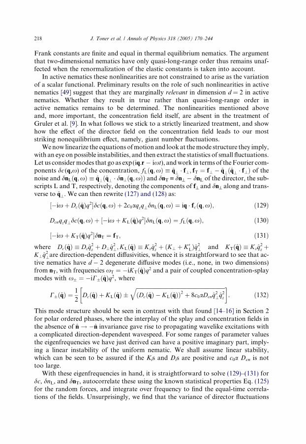
218 J. Toner et al. / Annals of Physics 318 (2005) 170–244
Frank constants are finite and equal in thermal equilibrium nematics. The argumentthat two-dimensional nematics have only quasi-long-range order thus remains unaf-fected when the renormalization of the elastic constants is taken into account.
In active nematics these nonlinearities are not constrained to arise as the variationof a scalar functional. Preliminary results on the role of such nonlinearities in activenematics [49] suggest that they are marginally relevant in dimension d = 2 in activenematics. Whether they result in true rather than quasi-long-range order inactive nematics remains to be determined. The nonlinearities mentioned aboveand, more important, the concentration field itself, are absent in the treatment ofGruler et al. [9]. In what follows we stick to a strictly linearized treatment, and showhow the effect of the director field on the concentration field leads to our moststriking nonequilibrium effect, namely, giant number fluctuations.
Wenow linearize the equations ofmotion and look at themode structure they imply,with an eye on possible instabilities, and then extract the statistics of small fluctuations.Let us considermodes that go as exp (iq.r � ixt), andwork in terms of theFourier com-ponents dc (q,x) of the concentration, fLðq;xÞ � q? � f?; fT ¼ f? � q?ðq? � f?Þ of thenoise and dnLðq;xÞ � q?ðq? � dn?ðq;xÞÞ and dnT ” dn^ � dnL of the director, the sub-scripts L and T, respectively, denoting the components of f^ and dn^ along and trans-verse to q?. We can then rewrite (127) and (128) as:
½�ixþ DcðqÞq2�dcðq;xÞ þ 2c0aqzq?dnLðq;xÞ ¼ iq � fcðq;xÞ; ð129Þ
Dcnqzq?dcðq;xÞ þ ½�ixþ KLðqÞq2�dnLðq;xÞ ¼ fLðq;xÞ; ð130Þ
½�ixþ KTðqÞq2�dnT ¼ fT; ð131Þwhere DcðqÞ � Dzq
2z þ D?q
2?;KLðqÞ � Kzq
2z þ ðK? þ K 0
LÞq2? and KTðqÞ � Kzq
2z þ
K?q2?are direction-dependent diffusivities, whence it is straightforward to see that ac-
tive nematics have d � 2 degenerate diffusive modes (i.e., none, in two dimensions)from nT, with frequencies xT ¼ �iKTðqÞq2 and a pair of coupled concentration-splaymodes with x� ¼ �iC�ðqÞq2, where
C�ðqÞ ¼1
2DcðqÞ þ KLðqÞ �
ffiffiffiffiffiffiffiffiffiffiffiffiffiffiffiffiffiffiffiffiffiffiffiffiffiffiffiffiffiffiffiffiffiffiffiffiffiffiffiffiffiffiffiffiffiffiffiffiffiffiffiffiffiffiffiffiffiffiffiffiffiffiffiffiffiDcðqÞ � KLðqÞð Þ2 þ 8c0aDcnq
2?q
2z
q� �. ð132Þ
This mode structure should be seen in contrast with that found [14–16] in Section 2for polar ordered phases, where the interplay of the splay and concentration fields inthe absence of n ! �n invariance gave rise to propagating wavelike excitations witha complicated direction-dependent wavespeed. For some ranges of parameter valuesthe eigenfrequencies we have just derived can have a positive imaginary part, imply-ing a linear instability of the uniform nematic. We shall assume linear stability,which can be seen to be assured if the Kis and Dis are positive and c0a Dcn is nottoo large.
With these eigenfrequencies in hand, it is straightforward to solve (129)–(131) fordc, dnL, and dnT, autocorrelate these using the known statistical properties Eq. (125)for the random forces, and integrate over frequency to find the equal-time correla-tions of the fields. Unsurprisingly, we find that the variance of director fluctuations

J. Toner et al. / Annals of Physics 318 (2005) 170–244 219
grows as 1/q2 at small wavenumber q (see [21] for details). Remarkably, as we havementioned above, this leads to a similar divergence
c0SðqÞ �Z
ddr
ð2pÞde�iq�rhdcð0; tÞdcðr; tÞi ¼ ð2c0aq?qzÞ
2Dn
F ðqÞq6 / 1
q2ð133Þ
in the static structure factor S (q) for concentration fluctuations, where
F ðqÞ � 2ðDcðqÞ þ KLðqÞÞ½DcðqÞKLðqÞ � 2c0aDcnq2?q
2z �. ð134Þ
This implies colossal concentration fluctuations at small q, diverging as 1/q2 in theentire nematic phase, comparable only to thermal equilibrium systems at a criticalpoint where where the compressibility diverges as q fi 0, i.e., in real space, as L2
for a system of linear dimension L. An additional feature in the systems of interesthere is that the singularity is strongly direction-dependent, vanishing both along andperpendicular to the ordering direction, but nonvanishing for all directions in be-tween. We have not considered what this means for response functions in the drivensystems of interest; it is not completely obvious how to formulate this, since responsefunctions require for their definition an underlying Hamiltonian, which one wouldneed to identify for each physical realization of active nematics. Regardless of therelation between response and correlation, it is an identity that
Sðq ! 0Þ ¼ hN 2i � hNi2
hNi
" #N!1
. ð135Þ
We see thus that (133) implies that the standard deviation rN / N12þ
1d and in partic-
ular for d = 2, as claimed earlier in this section, we see that rN � N, standard devi-ation proportional to the mean.
An effect as large as this should be measurable in experiments on active nematics,and would be a striking signal of their nonequilibrium nature. Two notes of cautionshould accompany this prediction, however. First, experimental realizations ofnematics, active or otherwise, generally require quite a high particle concentration.Detecting concentration fluctuations in such dense systems could require going tovery large system sizes (recall that the predictions we have made above are asymp-totic results for large N). Second, our mechanism for giant fluctuations is in similarin spirit to the work of Das et al. [50] on particles sliding downhill on fluctuating sur-faces with an invariance under uniform translations of the height field h. In activenematics, orientational fluctuations are soft and slowly relaxing because of sponta-neously broken rotation-invariance; in the surface problem, the symmetry ofh fi h+ constant means that the height field is a broken-symmetry mode. If we wereto carry out a simple linearized analysis of concentration fluctuations in the problemof [50], about a state with uniform concentration and height, we would find giantconcentration fluctuations with a divergent structure factor. The treatment of [50]shows that the system is actually unstable to coarsening, and the true statistical stea-dy state at infinite time is one with a delicate kind of macroscopic phase separation.It is unclear whether that is what must ultimately happen in active nematics too.There is an important difference between the two cases: the particle velocity in the
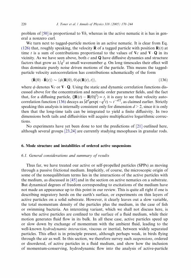
220 J. Toner et al. / Annals of Physics 318 (2005) 170–244
problem of [50] is proportional to $h, whereas in the active nematic it is has in gen-eral a nonzero curl.
We turn next to tagged-particle motion in an active nematic. It is clear from Eq.(126) that, roughly speaking, the velocity _R of a tagged particle with position R (t) attime t is a sum of contributions proportional to the values of $c and $ �Q in itsvicinity. As we have seen above, both c and Q have diffusive dynamics and structurefactors that grow as 1/q2 at small wavenumber q. On long timescales their effect willthus dominate purely noise driven motions of the particle. This means the tagged-particle velocity autocorrelation has contributions schematically of the form
h _Rð0Þ � _RðtÞi h/ðRð0Þ; 0Þ/ðRðtÞ; tÞi; ð136Þwhere / denotes $c or $ �Q. Using the static and dynamic correlation functions dis-cussed above for the concentration and nematic order parameter fields, and the factthat, for a diffusing particle, Æ|R (t) � R(0)|2æ � t, it is easy to see that velocity auto-correlation function (136) decays as �ddqexp(�q2t) t�d/2, as claimed earlier. Strictlyspeaking this analysis is internally consistent only for dimension d > 2, since it is onlythen that the long-time tails can be integrated to yield a finite diffusivity. In twodimensions both tails and diffusivities will acquire multiplicative logarithmic correc-tions.
No experiments have yet been done to test the predictions of [21] outlined here,although several groups [23,24] are currently studying mesophases in granular rods.
6. Mode structure and instabilities of ordered active suspensions
6.1. General considerations and summary of results
Thus far, we have treated our active or self-propelled particles (SPPs) as movingthrough a passive frictional medium. Implicitly, of course, the microscopic origin ofsome of the nonequilibrium terms lies in the interactions of the active particles withthe medium, as discussed in [45] and in the section on active nematics on a substrate.But dynamical degrees of freedom corresponding to excitations of the medium havenot made an appearance up to this point in our review. This is quite all right if one isdescribing migratory herds on the earth�s surface, or experiments on thin layers ofactive particles on a solid substrate. However, it clearly leaves out a slow variable,the total momentum density of the particles plus the medium, in the case of fishor swimming bacteria. An interesting variant, which we shall not discuss here, iswhen the active particles are confined to the surface of a fluid medium, while theirmotion generates fluid flow in its bulk. In all these case, active particles speed upor slow down by exchange of momentum with the ambient fluid, leading to thewell-known hydrodynamic interaction, viscous or inertial, between widely separatedparticles. This effect is in principle present, although perhaps weak, in birds flyingthrough the air as well. In this section, we therefore survey such suspensions, orderedor disordered, of active particles in a fluid medium, and show how the inclusionof momentum-conserving, hydrodynamic flow into the analysis of active-particle

J. Toner et al. / Annals of Physics 318 (2005) 170–244 221
systems introduces important qualitative departures from the behavior presented inthe preceding sections of this review.
The problem of the individual and collective swimming of organisms has long at-tracted the attention of fluid-dynamicists [51–53], However, we know of no workapart from [19,20] which attempts a general theory of ordered states and fluctuationstherein in the context of active particles suspended in a fluid. Part of the motivationthe work in [19,20] came from an original experiment [54] on correlated bacterialswimming in a freely suspended fluid film, which we will discuss briefly at the endof this section, along with more recent experiments [55].
The main results of the analysis of [19,20] illustrate the crucial role of the hydro-dynamics of the ambient fluid medium.
(A) If the role of viscosity is ignored, as should be the case for inertia-dominatedswimmers like fish, then the analysis of [19] predicts that apolar, purely nematic orderin active suspensions is always destabilized at small enough wavenumber q, by a cou-pled splay of the axis of orientation and a corresponding Taylor–Couette-like circu-lation of the velocity field, oriented near 45� to the nematic axis, with a growth ratelinear in q. Recall, by contrast, from Section 5 and [21] that, for active nematics on a
substrate, parameter ranges could always be found within which the phase wasdynamically stable. Small fluctuations about a state with polar order in an active sus-pensions travel as propagating waves, with a most elaborate dispersion relation (see[19]), as a result of the interplay of hydrodynamic flow and the concentration withbend, twist and splay of the director field. Again, there is an important qualitativedifference between these results and those obtained for polar-ordered phases of ac-tive particles on a substrate [14–16], as discussed in Section 2.3, where bend and twistdisplayed an overdamped rather than a propagating character.
(B) Bacterial suspensions are one natural testing ground for ideas on active-particle systems. The appropriate dynamical regime for these ubiquitous systemsis the Stokesian limit where viscous damping is dominant and inertia and accel-erations are ignored. In this important limit, it was shown in [19] that a suspen-sion in a state of uniform polar order, with nonzero mean drift velocity ~v0, isalways unstable for wavevectors q oriented near 45� to the ~v0, with a growth ratev0/a, for particles of size a, for Re � qa � /1/2, where / is the volume fractionof particles, and Re is the Reynolds number evaluated at the size of a particle.The instability is ‘‘convective’’: it travels with a speed v0 as it grows. This resulttells us that collections of coherently swimming bacteria cannot exceed a certainsize a/�1/2. It is likely that this instability has been seen in [55], although thelatter do not make a quantitative comparison between their observations andthe predictions of [19].
(C) Isotropic suspensions of active particles are of interest for their rheology[56,57], i.e., the response to imposed shear, and for the huge noise temperature theydisplay [54]. Ref. [20] offers a framework to understand these phenomena, account-ing for the large apparent temperature, predicting, as a result, hydrodynamic long-time tails with a greatly enhanced amplitude, and arguing that as the relaxation timefor orientational order increases, active suspensions should display viscoelasticity ofthe sort seen near translational arrest in equilibrium systems.

222 J. Toner et al. / Annals of Physics 318 (2005) 170–244
Lastly, number fluctuations in polar-ordered SPP suspensions are also shown tobe anomalously large. The purely linearized analysis in [19] predicts precisely thesame divergence as in active nematics on a substrate (Section 5 and [21]), viz.The variance Æ(dN)2æ in the number of particles, scaled by the mean N, is predictedto diverge as N2/d in d dimensions. This result is likely to be altered in detailonce nonlinear fluctuation effects are included, as in [14–16] for polar ordered sys-tems without fluid flow. Such an analysis has not yet been carried out for activesuspensions.
6.2. Equations of motion, modes, and instabilities
The equations of motion from which these results follow are straightforward toconstruct. We begin by identifying the slow variables. The local densities of con-served quantities in an active suspension are the coarse-grained number densityc (r, t) of active particles and the total (solute + solvent) momentum densityg (r,t) ” qu (r, t), where we take q, the mass density of the suspension as a whole—particles plus fluid—to be constant since the flows in question are far slower thanthe speed of longitudinal sound, and u is the hydrodynamic velocity field. The bro-ken symmetry variables, that is the director components dn^ perpendicular to themean ordering direction z, in uniaxial nematic or vector ordered phases have al-ready been discussed above in Sections 2 and 5. We use the same notation as inthose sections. The nematic phase is a traceless symmetric second-rank tensorQ (r, t); Qij � ninj�(1/3)dij where n is the unit director field. In the ordered phaseÆQ(r,t)æ ” Q0diag (�1,�1,2), Q0 „ 0. The presence of order in the vectorial phaseis indicated by a Galilean-invariant order parameter, the nonzero average driftvelocity h~vðr; tÞi ¼ ð0; 0; v0Þ relative to the fluid. Fluctuations about the vector or-dered state are expressed in terms of the director field as~v ¼ ð0; 0; v0Þ þ v0dn?. Whenconstructing the equations of motion we must keep in mind that the polar-orderedstate lacks the n ! �n invariance of the nematic.
We use once again the general principle that the nonequilibrium conditions obligeus to consider all terms not explicitly forbidden by symmetry or conservation, andthat all invariances are to be imposed directly on the equations of motion, withno ad hoc assumptions about the existence of a free-energy functional. We imposea priori no relations amongst the phenomenological parameters other than those de-manded by purely geometrical symmetries. The equations of motion follow quitesimply from these considerations.
For the polar-ordered case, the director field obeys an equation which combinesfeatures of the equations for polar order on a substrate with the flow-alignmentterms familiar from nematic hydrodynamics
otdn? ¼�k1v0ozdn?�r1$?dcþ1
2ðozu?�$?uzÞþ
1
2c2ðozu?þ$?uzÞþD$$dn?.
ð137ÞIn sequence, the first two terms on the right-hand side of (137), which arise in [14–16] and the discussion in Section 2, represents advection by the mean drift v0, and

J. Toner et al. / Annals of Physics 318 (2005) 170–244 223
a nonequilibrium ‘‘osmotic pressure,’’ the third and fourth together, absent in [14–16] and Section 2, are the well-known coupling of orientation to flow [18,58,59] ofnematic hydrodynamics, governed by the phenomenological parameter c2, and playa central role in this section, and the last term schematically denotes director dif-fusion.
As in any momentum-conserving system, the momentum density g of particlesplus fluid obeys
otg ¼ �$ � r; ð138Þwhere r is the stress tensor. The distinctive feature of active systems, as we pointedout in our discussion on active nematics on a substrate in Section 5, is a contributionto r / nn� I=d in d dimensions, where I is the unit tensor, arising from the activityof the particles. We already argued that such a term was inevitable in driven systemssimply because symmetry could not rule it out. Let us see how it arises in a moremicroscopic picture. Newton�s third law, that the active particles and the fluid exertequal and opposite forces on each other. Thus, in the equation of motion for the to-tal momentum density g, the force density associated with each active particle mustintegrate to zero, which means that it can have no monopole moment. Averagingover the internal motions that lead to activity and self-propulsion, we see that thesimplest model for, say, the ath active particle is a rod with axis naðtÞ, at time t, de-fined by a pair of equal and opposite point forces of magnitude f on its ends, directedalong �na [19]. Any real active particle will of course have higher multipoles in itsforce distribution as well, but the monopole will be absent. In addition real activeparticles will not in general be uniaxial, but we restrict ourselves for simplicity hereto uniaxial particles. A collection of uniaxial active particles with centers at ra (t) andends (in general asymmetrically disposed about the center) at ra þ ana and ra � a0na,lead to a force density (divergence of stress)
�r � rðpÞ � fðpÞðr; tÞ
¼ fXa
naðtÞ½dðr� raðtÞ � anaðtÞÞ � dðr� raðtÞ þ a0naðtÞÞ�. ð139Þ
The polar and apolar SPPs we mentioned in Section 1 correspond respectively toa „ a 0 and a = a 0. For obvious reasons, [20] terms the former ‘‘movers’’ and the latter‘‘shakers.’’ That this force–dipole picture of active particles is physically reasonablecan be seen by considering, as in [20], a simple model swimmer such as a bacteriumwith two flagella. This physical picture is realized as well in bundles of active fila-ments such as those found in the cytoskeleton [60].
Expanding the delta-functions in (139) about ra gives
f ðpÞi ’ � aþ a0
2frj
Xa
nainajdðr� raÞ þOðrrÞ ð140Þ
leading upon coarse-graining to an active contribution
raijðr; tÞ ¼
aþ a0
2fcðr; tÞ ninj �
1
3dij
�þOðrÞ ð141Þ

224 J. Toner et al. / Annals of Physics 318 (2005) 170–244
to the deviatoric (traceless symmetric) stress. This justifies in detail the claim that ac-tive stresses are proportional to the local nematic order parameter. It is interestingthat a and a 0 appear only in the symmetric combination a + a 0 in (141); to leadingorder in gradients, movers and shakers have the same active stress and hence thesame far-field fluid flow. A mover swims because the fluid velocity its activity inducesat its own center is nonzero; the corresponding quantity is zero by symmetry forshakers. This distinction is a property of the near field fluid flow.
Using the stress (141) in the momentum Eq. (138), linearizing, Fourier-transform-ing in space, writing g = qu, and projecting transverse to the wavevector q to imposeincompressibility ($ Æ u = 0) yields
ou?
ot¼ �iw0qz I� 2
q?q?q2
�.dn? � i
q2zq2
aðq?dcÞ þ g$$u?; ð142Þ
where g is a viscosity tensor, I is the unit tensor, and a fa/q and w0 c0 a are phe-nomenological constants proportional to the activity of the SPPs. In (142), nematicelastic torques [18], which are subdominant at small q, have been ignored, as haveinertial and other nonlinearities. The presence of forces from concentration gradients(the pressure-like a term) in an incompressible system, and the acceleration propor-tional to the bend qzdn^, are key features arising entirely because of nonequilibriumactivity.
Expanding the continuity equation otdc = �$ Æ j for the concentration for smallfluctuations about the uniform ordered state, where the current j ¼ cv0n apart fromadvection by fluid flow. To leading order this leads to
ðot þ v0ozÞdcþ c0v0r? � dn? ¼ 0 ð143Þwhich contains advection by the mean drift v0 and the nonequilibrium effect of localsplay.
The propagating waves and instabilities mentioned at the start of this section fol-low from (137), (142), and (143) by considering, once again, disturbances varying asexp(iq Æ r � ixt), and assuming small wavenumber. Briefly, the coupled dynamics ofbend or twist ð$� n?Þ and vorticity along z, ð$� u?Þ, leads, from (137) and (142) to‘‘bend-twist’’ waves with wavespeeds
cbtðhÞ ¼ ðc1 � c2Þ cos h; ð144Þwhere h is the angle between the propagation vector and the ordering direction, andc1 and c2 (of order the drift speed v0 of the SPPs) are phenomenological constants.The corresponding modes in [14–16] were purely diffusive, thus highlighting theimportance of fluid flow. Taking instead the divergence of (137) and (142) resultsin coupled equations of motion for splay $ � n?, dilation in the xy plane $ � u?,and concentration fluctuations dc. The resulting wavelike eigenmodes are a rathercomplicated generalization of those seen in the flocking problem on a substrate[14–16], with wavespeeds determined by the solution to a cubic equation. All thatreally matters here is that one can show that there exists a finite range of parametervalues in which the wavespeeds are real in all directions, i.e., that the system is notinevitably dynamically unstable. The speeds as functions of direction, for typical

Fig. 13. Sketch of the speeds of propagating modes arising from the coupling of splay, concentration, andthe x–y-plane dilation. The speed in a particular direction h relative to the axis of orientation is thedistance from the origin to the curve(s) in that direction.
J. Toner et al. / Annals of Physics 318 (2005) 170–244 225
parameter values, can be found in [19], and are plotted in Fig. 13. In all the abovepropagating modes, the damping, for small values of viscosity, is of order q2.
Systems at low Reynolds number, for example bacteria, are an altogether differentstory. Their speeds v0 are so low that one is in practice always in the wavenumberrange where gq2 � qv0q. We can then use the Stokesian approximation, where thevelocity field u is determined instantaneously by a balance between viscous and stres-ses stresses. We can thus discard the acceleration in (142) in favor of the viscousdamping term, solve for u in terms of concentration and director fields, and use thissolution in (137) and (143). This yields effective equations of motion for the coupleddynamics of splay $ Æ dn^ and dc, leading to an eigenfrequency with imaginary part
CðhÞ Bðc2 cos 2hþ 1Þ cos 2h ð145Þwith |B| f//a2g v0//a, / being the volume fraction of active particles. Since theC = 0 for h = p/4, it must be positive (i.e., unstable) just above or just below h = p/4,depending on the sign of B. The frequency still has a nonzero real part ± v0qcosh:this is a convective instability, which is seen if one follows the traveling waves. Notethat C is independent of the magnitude of q, as a result of the long-ranged hydrody-namic interaction in the Stokesian limit. Some algebra will show that for qa J /1/2,diffusivities of particles and director restabilize the mode, so the instability exists forRe � qa � /1/2. Thus, if the volume fraction is not too high, there should be a rangeof length scales over which vectorial order can still exist in bacterial suspensions.However, on scales of a few particle sizes, the instability should set in. It appearslikely that this instability has been seen in [55], but a quantitative analysis of theirexperiment is awaited.
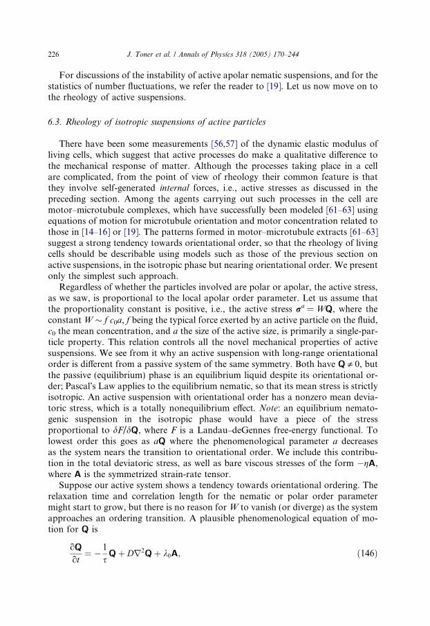
226 J. Toner et al. / Annals of Physics 318 (2005) 170–244
For discussions of the instability of active apolar nematic suspensions, and for thestatistics of number fluctuations, we refer the reader to [19]. Let us now move on tothe rheology of active suspensions.
6.3. Rheology of isotropic suspensions of active particles
There have been some measurements [56,57] of the dynamic elastic modulus ofliving cells, which suggest that active processes do make a qualitative difference tothe mechanical response of matter. Although the processes taking place in a cellare complicated, from the point of view of rheology their common feature is thatthey involve self-generated internal forces, i.e., active stresses as discussed in thepreceding section. Among the agents carrying out such processes in the cell aremotor–microtubule complexes, which have successfully been modeled [61–63] usingequations of motion for microtubule orientation and motor concentration related tothose in [14–16] or [19]. The patterns formed in motor–microtubule extracts [61–63]suggest a strong tendency towards orientational order, so that the rheology of livingcells should be describable using models such as those of the previous section onactive suspensions, in the isotropic phase but nearing orientational order. We presentonly the simplest such approach.
Regardless of whether the particles involved are polar or apolar, the active stress,as we saw, is proportional to the local apolar order parameter. Let us assume thatthe proportionality constant is positive, i.e., the active stress ra = WQ, where theconstantW f c0a, f being the typical force exerted by an active particle on the fluid,c0 the mean concentration, and a the size of the active size, is primarily a single-par-ticle property. This relation controls all the novel mechanical properties of activesuspensions. We see from it why an active suspension with long-range orientationalorder is different from a passive system of the same symmetry. Both have Q „ 0, butthe passive (equilibrium) phase is an equilibrium liquid despite its orientational or-der; Pascal�s Law applies to the equilibrium nematic, so that its mean stress is strictlyisotropic. An active suspension with orientational order has a nonzero mean devia-toric stress, which is a totally nonequilibrium effect. Note: an equilibrium nemato-genic suspension in the isotropic phase would have a piece of the stressproportional to dF/dQ, where F is a Landau–deGennes free-energy functional. Tolowest order this goes as aQ where the phenomenological parameter a decreasesas the system nears the transition to orientational order. We include this contribu-tion in the total deviatoric stress, as well as bare viscous stresses of the form �gA,where A is the symmetrized strain-rate tensor.
Suppose our active system shows a tendency towards orientational ordering. Therelaxation time and correlation length for the nematic or polar order parametermight start to grow, but there is no reason for W to vanish (or diverge) as the systemapproaches an ordering transition. A plausible phenomenological equation of mo-tion for Q is
oQ ¼ � 1Qþ Dr2Qþ k0A; ð146Þ
ot s

J. Toner et al. / Annals of Physics 318 (2005) 170–244 227
where s is a relaxation time, D is a diffusivity proportional, at equilibrium, to the ra-tio of a Frank constant to a friction constant, k0 is a flow-alignment, and A is thesymmetrized strain-rate tensor. From the preceding discussion, we see that this leads,for sinusoidally oscillating stresses and strains � exp(�ixt), to
rxyðxÞ ¼ � g0 þðaþ W Þk0�ixþ s�1
� �Axy � �G0ðxÞ � iG00ðxÞ
xiAxy . ð147Þ
Eq. (147) predicts strong viscoelasticity as s increases. Note first that for passive(equilibrium) systems, W = 0. Since a � s�1 decreases as the system approaches anordering transition, G 0 (xs � 1) decreases as k0g0/s. There is not much viscoelasticitynear an equilibrium isotropic–nematic transition. For active systems, as we said, W isprimarily a single-particle property, independent of s and of proximity to the tran-sition. Thus, as s grows
G0ðxs � 1Þ ’ W ð148Þindependent of s and, of course, the dynamic range over which elastic behavior isseen increases. This is classic Maxwell viscoelasticity, normally expected at equilib-rium near translational not orientational ordering. The ideas on rheology proposedhere have not been tested, although there has been one set of experiments [64] onoptically trapped beads in a bacterial suspension in which the strength of the trap-ping potential was modulated. It is not obvious how to relate the theoretical devel-opments in this section to that particular type of modulation, which is quite distinctfrom the microrheological measurements of, e.g. [57].
Lastly, in the isotropic phase, in the absence of imposed shear, the active stresscan simply be thought of as an added noise in the momentum Eq. (138). The noisetemperature corresponding to the active stress can be estimated on dimensionalgrounds: the variance of ra (k = 0,x = 0) is W2n3s, with W gu0/n for active par-ticles moving with typical speed u0, correlated over a scale n and time s. We can de-fine the effective temperature by equating this stress variance to kBTeffg. If we takeg gwater = 0.01 poise, u0 to be a bacterial swimming speed 20 lm/s, and s 1 s(an Escherichia coli run time) we get a noise temperature Teff 105–106 K. This isconsistent with the findings of [54]. More remarkably, it will will mean a thousand-fold enhancement of the t�d/2 long-time tails [40] in the autocorrelation of tagged-particle velocities.
7. Comparison with past experiments
7.1. Anomalous diffusion near the order–disorder transition
With a fair amount of information accumulating for the flocking models, it is nat-ural to ask where one can test the predictions from the flocking models againstbehaviors of real experimental systems. Even though the theory can be easily moti-vated by macroscopic flocking systems, such as bird flocks and fish schools, the mostlikely systems to test the flocking theory in a controllable fashion are probably

228 J. Toner et al. / Annals of Physics 318 (2005) 170–244
micro-organism where collective behaviors are often observed. In particular, it isprobably easiest to eliminate external aligning fields in bacterial systems, whereasin fish or birds, ocean currents, winds, the earth�s magnetic field, the sun, etc., areimpossible to get rid of. Bacteria such as E. coli exhibit fascinating collective behav-ior in liquid media. It has been observed that they form jets and swirls even in theabsence of any external stimulus. How can one characterize and explain such spatialand temporal collective behavior? Recently, Wu and Libchaber (WL) [54] reportedon a fascinating experiment in which bacteria move freely within a fluid film seededwith polystyrene beads whose motion was recorded. They studied the dynamics ofthese beads as they are moved around by the bacteria, and found superdiffusive mo-tion (Ær2æ ta with a . 1.5) below some crossover scales tc, ‘c, beyond which normaldiffusion (a = 1) is recovered. For related work, in a three-dimensional geometry, see[65]. WL interpreted these scales as characteristic of the structures (swirls, jets) thatemerge from the collective motion of the bacteria. A simple Langevin equation witha force term correlated in time over the crossover scale tc was used to fit the exper-imental data. Two problems arise from this description: first, the Langevin frame-work predicts ballistic behavior (a = 2) at short scales, at odds with the nontrivialexponents recorded in the experiment. Second, no attempt is made to explain the ori-gin of the collective motion and how/why the crossover scales change with the bac-teria density q.
In an alternative approach, Gregoire et al. [66] proposed to model the system byusing flocking model for describing the bacteria motion, complemented by a simplemodel describing the motion of the passive (polystyrene) beads. In this model, bac-teria move at discrete time steps with fixed-amplitude velocity v0 along a directionreflecting the action of two forces: a noisy tendency to align with neighboring objectswithin a radius R, and a two-body repulsive force giving them an effective size rb. Asmall number of passive beads of radius rB is added. They interact with bacteria viahard-core repulsion plus some level of entrainment within range R (i.e., they takepart of the neighboring bacteria velocity). The results from this ‘‘passive beads ina active boids bath’’ model are shown in Fig. 14.
Increasing the bacteria density q, ordered collective motion appears at a value q*.For q < q*, bacteria motion is characterized by scales which increase as q fi q* (Fig.14A). The bead motion is directly related to the behavior of the bacteria, as shownby their respective diffusive properties which both reveal superdiffusion crossing overat the same timescale tc to normal diffusion (Figs. 14B and C). The characteristicscales of bead motion are thus given by the collective scales of bacteria motion, asforeseen by WL, but the short-time behavior of the beads in the flocking model issuperdiffusive, which is more consistent with the experimental data than the simpleLangevin Ansatz.
The density dependence of the crossover scales is also naturally explained by thismodel: as q increases, the system is closer to the critical point q*, and the superdif-fusive behavior persists longer. The range of variation of crossover scales recordedby WL is small (e.g., the maximum value of ‘c is of the order of rB), this explainswhy a linear variation was found to be a good approximation in [54], even thoughthe scales are expected to diverge at threshold (Fig. 14C). The physical picture

Fig. 14. The flocking model for bacterial bath with passive beads with v0 = 0.3, r0 = 1.0, rb = 0.13, andrB = 0.38 (for other details, see [66]). (A) Short-time (30 timesteps) trajectories of bacteria (thin lines) andbeads (thick lines) for q < q* in a system of size 32 · 32; (B) mean square displacement Ær2æ versus time forbacteria (solid lines) and beads (dashed lines) for q = 2,3, 3.5 < q* . 4.2; (C) q-variation of tc (squares)and ‘c (triangles) and diffusion constant D = limtfi1dÆr2æ/dt (s); (D) superdiffusion at q = q* withexponent a. 1.65 ± 0.15.
J. Toner et al. / Annals of Physics 318 (2005) 170–244 229
emerging from the flocking model is rather simple. As the density of bacteria in-creases, the aligning interaction between cell motion becomes stronger, and bacteriaform finite clusters that move coherently for a finite time before they dissolve into therandom background; the polystyrene beads join and leave these coherent dynamicalstructures passively and, as a result, follow a motion composed of random steps ofvarious sizes (Levy flight), leading to a nontrivial superdiffusive behavior up to atimescale set by the coherent structures of the bacteria cells.
Even though phenomenologically the results from the flocking model are consis-tent with the superdiffusive scaling behavior and its density dependence, the mecha-nism for the required velocity alignment interaction is totally unknown. To formcoherent structure, such as swirls and jets, there has to be intercellular interactionsbetween bacteria. Whether such interaction is mediated chemically (by bacterial

230 J. Toner et al. / Annals of Physics 318 (2005) 170–244
chemotaxis) or physically (through the fluid media) or both remains a very interest-ing challenge in biology. The readers are reminded to check out the related discus-sion in Section 5 in the context of a model [19] that includes the hydrodynamics ofthe ambient fluid in which the bacteria move. Whether the anisotropic rod like shapeof the E. coli cell plays any role in the alignment of the cells is also an interestingquestion. Only when the nature of the cell–cell interaction become clear, can weknow definitively whether flocking model is appropriate for describing the system.
7.2. Pattern formation in finite system: the vortex state
We have so far emphasized the bulk properties of the flocking system. In reality,however, flocks are finite and boundary effects can be important. One natural ques-tion is whether interesting spatial patterns, such as the beautiful rings formed by fishschools, could be explained by the same type of flocking model with finite numberof self propelled particles. We shall focus in this section of the work of [3,4] whichinvestigates this question both experimentally and theoretically in D. discoideum, thecellular slime mould. Vortices (concentric circles), asters (radial spokes), and spirals(a combination of the two) were also displayed in the experiments of Nedelec et al.[67] on cell extracts containing molecular motors, the microtubules on which theywalk, and ATP to fuel them. Lee and Kardar [61], inspired by the experiments of[67], formulated a model similar to those of [14,16], for the coupled dynamics of mo-tor concentration and microtubule orientation. This was extended and crucially im-proved by Sankararaman et al. [62], who included in particular the pressure term wediscuss in the present paper. Kruse et al. [63] analyze the experiments of [67] in aframework which includes the hydrodynamic flow of the ambient fluid in the cell,using a model closely related to that of [19,20], and find that spirals in their model,as in the experimental systems of [67], are always accompanied by a circulation ofthe fluid flow.
We restrict our attention here to [3,4], where Dictyostelium cells were first grownin liquid media and then placed onto a glass surface with an additional layer of aga-rose overlaid on the cells, which restrict the cell motion to the plane. It was foundthat the cells aggregate and form a two-dimensional round structure (‘‘pancake’’)in which the cells have organized into a coordinated vortex state rotating aroundthe center of the pancake. More interestingly, the same behavior was also observedin a nonsignaling strain of Dictyostelium, in which long-range communicationthrough cyclic adenosine 3 0–5 0 monophosphate (cAMP) is absent. Thus guidancethrough a global variable, such as cAMP, is ruled out as the cause for the organizedrotational motion. Instead the vortex state is most likely the result of self-organiza-tion due to local cell–cell interactions, analogous to the alignment interaction in theflocking models.
Indeed, in the accompanying and subsequent theoretical works by the samegroup[3,4], the system was modeled as a group of self-propelled cells, whose propul-sive and adhesive forces both depend on the interactions with neighboring cells. Withproper choice of parameters, the same type of vortex state was observed without theenforcement of any physical boundary. In the simpler model proposed in their

J. Toner et al. / Annals of Physics 318 (2005) 170–244 231
second paper [4], the model is almost the same as the continuum equations studied in[14,16] with the pressure term determined by summing over all pairwise boid–boidinteractions of a specific form. The resulting structure is a self-organized annulus,with a specific density profile, where the boid density drops abruptly to zero at boththe inner and outer boundary of the annulus. The velocity profile is featureless withits value almost fixed at its preferred value determined by the amplitude of the pro-pulsion and the friction coefficient.
For the simple Vicsek model with nearest neighbor cohesive force, such a self-organized vortex state has also been observed [37]. However, it only exists atparameters near the moving–nonmoving phase boundary, and the rotational direc-tion of the vortex state only persists for finite time before it changes to the oppositedirection. Several differences between the discrete model used in [4] and the simpleVicsek model are worth noticing. In [4], the boids have inertia and they do notchange their direction of motion completely according to their neighbor�s movingdirections, whereas the model by Vicsek et al. is overdamped. Perhaps a moreimportant difference is that the length scale (la) for the specific body forces usedin [4] is much larger than the actual distance between two nearest neighbor boids;in fact, the thickness of the annulus in the simulation shown in [4] is comparable tola, which means that essentially all the boids in the system interact with each other.It would be interesting to understand if and how any of these differences are rel-evant for the stability of the vortex state. As far as an understanding of the pat-terns and behavior of finite flocks in concerned, one key challenge, clearly, ishow to formulate the (free) moving boundary problem. In particular, it is crucialto understand the coexistence of boid-rich and boid-poor regions, the nature of theinterface between them, i.e., the free surface of the flock, and the nonequilibriumanalog of surface tension.
8. Suggestions for future experiments
In this section, we discuss how our theory can be tested in simulations and directobservations of real flocks. The ‘‘real’’ flocks may include, e.g., artificial self-pro-pelled particles such as those suggested in [10] or [68] which it should be possibleto build in the laboratory as well as aggregates of genuinely living organisms.
We begin with a few suggestions about the best boundary conditions and param-eter values for simulations or experiments, and then describe how the correlationfunctions and scaling exponents v, z, and f predicted by our theory can be measured.The most useful boundary conditions are ‘‘torus’’ conditions; that is, reflecting wallsin d � 1 directions, and periodic boundary conditions in the remaining direction, callit y (see Fig. 15). The advantage of these conditions is that one knows a priori that, ifthe flock does spontaneously order, its mean velocity will necessarily be in the peri-odic (y) direction.
It might be objected that imposing such anisotropic boundary conditions breaksthe rotation invariance our model requires, but this is not, in fact, the case. A ‘‘bird’’deep inside the box moves with no special direction picked out a priori; it can only

Fig. 15. Illustration of the optimal boundary conditions for simulations and experiments to test ourpredictions. The top and bottomwalls are reflecting, while periodic boundary conditions apply at the left andright walls (i.e., a bird that flies out to the right instantly reappears at the same height on the left). The meandirection of spontaneous flock motion, if any occurs, is clearly forced to be horizontal by these boundaryconditions. In spatial dimensions d > 2, one should choose reflecting boundary conditions in d � 1directions, and periodic in the remaining direction, thereby forcing h~vi to point along that periodic direction.
232 J. Toner et al. / Annals of Physics 318 (2005) 170–244
find out about the breaking of rotation invariance on the boundary if the bulk of theflock spontaneously develops long range order. This is precisely analogous to theway one speaks of a ferromagnet as spontaneously breaking a continuous symmetryeven if it orders in the presence of ordered boundary conditions.
So, by imposing these boundary conditions, we know the direction of the flockmotion (the y direction in the simulation), and, therefore, have oriented the simula-tion axes with the axes used in our theoretical discussion; i.e., our i axis equals thesimulation�s periodic direction.
Alternative boundary conditions add the additional complication of having tofirst determine the direction of mean flock motion before calculating correlationfunctions. This complication is even worse for a finite flock (as any simulation musttreat), since the mean direction of motion will wander, executing essentially a ran-
dom walk that will explore the full circle in a time of order T Flock ¼ 2pffiffiffiND
q. Our re-
sults, which assume a constant direction of flock motion, will only apply fortimescales t � TFlock. Even drifts of the mean flock direction through angles �2pcan cause problems, however, since most of the interesting scaling behavior is con-centrated in a narrow window of angles qk qf? � q?; i.e., near the direction ofmean flock motion. So this drift greatly complicates the experimental analysis, andis best avoided by using the toroidal boundary conditions just described.
Of course, it is considerably harder to produce these boundary conditions in a realexperiment. Ants walking around a cylinder may come close, although gravity willalways break rotation invariance on a real cylinder. Perhaps the experiment couldbe done on the space shuttle, or with a rapidly spinning cylinder producing artificialgravity that swamps real gravity, or by using neutrally buoyant organisms in a fluid.Alternatively, one could use a ‘‘track’’ such as that shown in Fig. 16, and take data

Fig. 16. More practical ‘‘track’’ geometry for experiments on real flocks. Data should only be taken fromthe cross-hatched region centered on the middle of the ‘‘straightaway.’’
J. Toner et al. / Annals of Physics 318 (2005) 170–244 233
only from the cross-hatched region, chosen to be in the middle of the straight sectionof the track, far from the curves.
Other, more ingenious ways to pre-pick the direction of mean motion throughboundary conditions may also be dreamed up by experimentalists more clever thanwe are.
We strongly caution anyone attempting to test our results, however, that it is onlythrough boundary conditions that one may pre-pick the direction of mean motion.Any approach that pre-picks this direction in the bulk of the flock, such as givingeach bird a compass, letting them be blown by a wind, or run downhill, or followa chemical scent, etc., will lead to a model outside the universality class of our isotro-pic model, since the starting model does not have any rotation invariance to be spon-taneously broken (unless the anisotropy leaves an ‘‘easy plane’’ in which alldirections are equivalent, in which case our anisotropic model of Section 3 applies).Indeed, such flocks of ‘‘birds with compasses’’ will be less interesting than the modelswe have studied here, since the ‘‘compass’’ will introduce a ‘‘mass’’ that makes anyfluctuation away from the pre-picked direction of flock motion decay rapidly (i.e.,nonhydrodynamically) with time. In such a model, it is easy to show that the non-linearities are irrelevant, and there are no interesting fluctuations left at long dis-tances and times.
Experiments to date on strictly apolar nematic phases of active particles have beenrather limited. The studies in [9] on nematic phases of melanocytes do not ask ques-tions about fluctuation statistics. The work of Kudrolli and co-workers [22,44], onagitated layers of granular rods, mentions a nematic phase but does not attemptto obtain macroscopic aligned domains. It focuses instead on the state where therods tilt out of the plane, thus turning into polar particles. Unpublished studiesshowing unambiguously nematic states in granular-rod systems include recent workby Fraden et al. [24] and Narayan et al. [23]. Until recently, however, no tests hadeven been attempted of the predictions we summarized in section of giant numberfluctuations (far larger than those in the ferromagnetic flocks) and 1/t long-time tailsin two dimensions of [21]. The work of [23] does show indications of anomalouslylarge concentration fluctuations. This is, however, preliminary, and awaits confirma-

234 J. Toner et al. / Annals of Physics 318 (2005) 170–244
tion by detailed quantitative analysis. Such analysis is currently in progress. Anotherpromising system on which to look for orientational order in active systems would bea layer of actin filaments on a flat substrate on which actin had been grafted or dis-tributed, in the presence of ATP [69]. At large enough actin concentration, mesopha-ses (apolar or polar?) should form, whose properties should be governed by ourequations in Sections 2 or 5.
Testing the properties of hydrodynamically interacting ordered active suspensionsrequires an obliging school of fish or flock of bacteria. The former would in principlebe the right system to test the rather complicated propagating mode structure pre-dicted in Section 6 and [19]. Probably more feasible is to enter the Stokesian regime:start with a a collection of bacteria such as those in [54] or [55], at high enough con-centration to form a polar ordered state. Prepare the system in the presence of animposed flow or chemical gradient to enforce an initial ordered state, then switchoff the imposed field and see if the ordered state breaks up in accordance with thepredictions of [19] and Section 6, with an instability wavevector just above or justbelow 45� to the ordering direction. More effective would be a detailed test in anumerical simulation of Stokesian swimming hard rods with Brownian motion[70]. The flagella could be deliberately so designed as to make polar or apolar par-ticles (‘‘movers’’ or ‘‘shakers’’). Such systems could be prepared in an initial statein which the flagellar motion or the force-densities imitating such motion wasswitched off, and excluded volume interactions resulted in an equilibrium nematicphase. Upon switching on the swimming, the instability (of either the apolar orthe polar suspension, depending on how the flagellar motion had been put in) shouldset in and its entire dynamical evolution can be examined in detail and compared tothe theory in [19].
The predictions of strong viscoelasticity in active isotropic suspensions should betestable in rheometry on bacterial or motor–microtubule suspensions at large en-ough concentration to be near the onset of an ordered phase.
And now a few words about parameter choices. For definiteness, we will discussin what follows the Vicsek model, whose parameters are v0 = S/R0, where S is thedistance the birds travel on each time step and R0 is the radius of the circle of neigh-bors, the mean number density q0 in units of 1
Rd0
where d is the dimension of the sys-tem, and the noise strength D, which is the mean squared angular error. Since theinteresting nonlinear effects in our model come from terms proportional to v20, thoseeffects will become important at shorter length scales in a faster moving flock. Thatis, in, e.g., the Vicsek model, should we chose the dimensionless velocity as large aspossible, consistent with the flock ordering. However, if we take v0 too big, i.e.,v0 � 1, then, on each time step, each bird is likely to have a completely differentset of neighbors. It is difficult to see how order can develop in such a model. So,to take v0 as big as possible without violating v0 � 1, we should chose v0 1. Thesimulations of Vicsek et al. [5] took v0 � 1, and, hence, probably never explored(in their finite flocks) the long length scale regime in which our nonlinear effects be-come important.
Now to the mean density q0, which is, of course, just determined by the total num-ber of birds N and the volume V of the box via q0 = N/V. We clearly want this to be
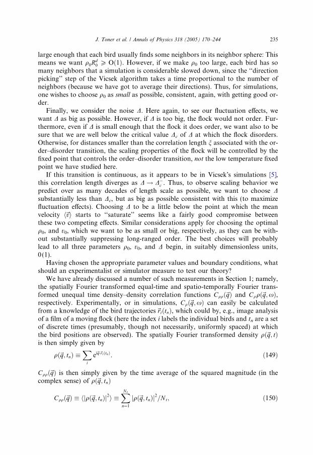
J. Toner et al. / Annals of Physics 318 (2005) 170–244 235
large enough that each bird usually finds some neighbors in its neighbor sphere: Thismeans we want q0R
d0 P Oð1Þ. However, if we make q0 too large, each bird has so
many neighbors that a simulation is considerable slowed down, since the ‘‘directionpicking’’ step of the Vicsek algorithm takes a time proportional to the number ofneighbors (because we have got to average their directions). Thus, for simulations,one wishes to choose q0 as small as possible, consistent, again, with getting good or-der.
Finally, we consider the noise D. Here again, to see our fluctuation effects, wewant D as big as possible. However, if D is too big, the flock would not order. Fur-thermore, even if D is small enough that the flock it does order, we want also to besure that we are well below the critical value Dc of D at which the flock disorders.Otherwise, for distances smaller than the correlation length n associated with the or-der–disorder transition, the scaling properties of the flock will be controlled by thefixed point that controls the order–disorder transition, not the low temperature fixedpoint we have studied here.
If this transition is continuous, as it appears to be in Vicsek�s simulations [5],this correlation length diverges as D ! D�
c . Thus, to observe scaling behavior wepredict over as many decades of length scale as possible, we want to choose Dsubstantially less than Dc, but as big as possible consistent with this (to maximizefluctuation effects). Choosing D to be a little below the point at which the meanvelocity h~vi starts to ‘‘saturate’’ seems like a fairly good compromise betweenthese two competing effects. Similar considerations apply for choosing the optimalq0, and v0, which we want to be as small or big, respectively, as they can be with-out substantially suppressing long-ranged order. The best choices will probablylead to all three parameters q0, v0, and D begin, in suitably dimensionless units,0 (1).
Having chosen the appropriate parameter values and boundary conditions, whatshould an experimentalist or simulator measure to test our theory?
We have already discussed a number of such measurements in Section 1; namely,the spatially Fourier transformed equal-time and spatio-temporally Fourier trans-formed unequal time density–density correlation functions Cqqð~qÞ and Cqqð~q;xÞ,respectively. Experimentally, or in simulations, Cqð~q;xÞ can easily be calculatedfrom a knowledge of the bird trajectories~riðtnÞ, which could by, e.g., image analysisof a film of a moving flock (here the index i labels the individual birds and tn are a setof discrete times (presumably, though not necessarily, uniformly spaced) at whichthe bird positions are observed). The spatially Fourier transformed density qð~q; tÞis then simply given by
qð~q; tnÞ �Xi
ei~q�~riðtnÞ. ð149Þ
Cqqð~qÞ is then simply given by the time average of the squared magnitude (in thecomplex sense) of qð~q; tnÞ
Cqqð~qÞ � hjqð~q; tnÞj2i �XNt
n¼1
jqð~q; tnÞj2=Nt; ð150Þ

236 J. Toner et al. / Annals of Physics 318 (2005) 170–244
where Nt is the total number of time steps averaged over. With qð~q; tÞ in hand,Cqqð~q;xÞ can also be obtained in a real experiment by by first calculating the spat-io-temporally Fourier transformed density
qnð~q;xÞ ¼Xðnþ1Þs
t¼ns
qnð~q; tÞe�ixt; n ¼ 0; 1; 2; . . . ð151Þ
over a set of long ‘‘bins’’ of time intervals of length s � t0 (the ‘‘microscopic’’ timestep), and then averaging the squared magnitude jqð~q;xÞj2 over bins
Cqqð~q;xÞ �Xnmax
n¼0
jqð~q;xÞj2
nmax
. ð152Þ
Our predictions for these correlation functions are given in Eqs. (73) and (32).One additional correlation function that can be measured quite easily is the mean
squared lateral displacement of a bird
w2ðtÞ � hj~x?i ðtÞ �~x?i ð0Þj2i ð153Þ
perpendicular to the mean direction of motion of the flock. This can easily be mea-sured as a function of time in a simulation or experiment simply by labeling a set of nbirds in a ‘‘strip’’ near the center of the channel with its long axis running parallel tothe mean direction of bird motion (see Fig. 17), and then following their subsequentmotion. It is best to center the strip in the channel so as to postpone the birds reach-ing the reflecting walls as long as possible. Once they do reach the walls, of coursew2 (t fi 1) saturates at L2
?, L^ being the width of the channel. We will deal in
Fig. 17. Illustration of the experiment to measure the mean squared lateral wandering w2 (t). One labels allof the birds some central stripe (of width�L, the channel width), and then measures the evolution of theirmean displacements ~x?ðtÞ perpendicular to the mean direction of motion (which mean direction ishorizontal in this figure).

J. Toner et al. / Annals of Physics 318 (2005) 170–244 237
the following discussion with times much smaller than that required for a bird at thecenter of the channel to wander out to its edge.
As shown in [16], we need to distinguish two cases:
[Case (1): 2vf > �1.] In this case, which holds in d = 2, where v = �1/5 and f = 3/5,
w2ðtÞ / t2ð1þvfÞ ¼ t4=3;
2vf> �1 ð154Þ
the last equality holding in d = 2. Note that this behavior is ‘‘hyperdiffusive’’: themean squared displacement w2 (t) grows faster than it would in a simple randomwalk; i.e., faster than linearly with time t.
[Case (2): 2vf < �1.] In this case, which certainly holds for d > 4 (where
v ¼ 1� d2< �1 and f = 1), we get
w2ðtÞ / t;2vf< �1. ð155Þ
Unfortunately, the analogous calculation for the anisotropic model shows that thisrandom ‘‘transverse walk’’ is much less interesting: for d < 5/2, which of course ex-cludes the physically interesting case d = 3, there is no hyperdiffusive behavior;rather, we expect w2 (t) � t. For the only other physically interesting case, namelyd = 2, the anisotropic model is the same as the isotropic model. This negative predic-tion could be checked experimentally, although its confirmation, while a nontrivialcheck of our theory, would clearly be less exciting than verification of our hyperdif-fusive prediction w2 (t) � t4/3 for the isotropic d = 2 model.
Some of the numerical tests discussed in this section have been carried out, par-ticularly on the d = 2 model, and good agreement with our prediction has beenfound, as described in Section 3 and [15].
9. Future directions
It should be obvious that the theoretical work we have reviewed in this paper is justthe tip of an enormous iceberg.As described in Section 1, there is every reason to expectthe behavior of flocks to be as rich as that of equilibrium condensedmatter systems. Inparticular, this means that virtually every one of the dozens of phases known in equi-librium systems probably has an analog in flocks. Indeed, virtually every question onecan ask about any equilibrium system can be asked about flocks. Here wewill present avery abbreviated list of a fewof the interestingquestions andproblems that remainwideopen. Anyone can easily add to this list by substituting one�s favorite phenomenon orphase from equilibrium systems and asking what is the analog in flocks.
9.1. Other phases of flocks
As we have seen in this review, only two phases of flocks (the ferromagnetic andthe nematic) have been extensively studied so far. There is every reason to expect that
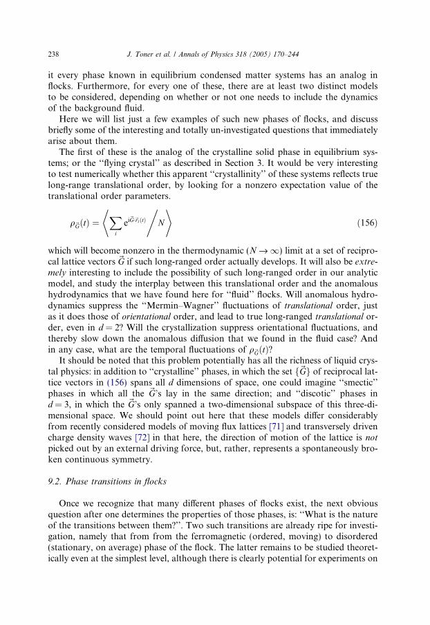
238 J. Toner et al. / Annals of Physics 318 (2005) 170–244
it every phase known in equilibrium condensed matter systems has an analog inflocks. Furthermore, for every one of these, there are at least two distinct modelsto be considered, depending on whether or not one needs to include the dynamicsof the background fluid.
Here we will list just a few examples of such new phases of flocks, and discussbriefly some of the interesting and totally un-investigated questions that immediatelyarise about them.
The first of these is the analog of the crystalline solid phase in equilibrium sys-tems; or the ‘‘flying crystal’’ as described in Section 3. It would be very interestingto test numerically whether this apparent ‘‘crystallinity’’ of these systems reflects truelong-range translational order, by looking for a nonzero expectation value of thetranslational order parameters.
q~GðtÞ ¼Xi
ei~G�~riðtÞ
* ,N
+ð156Þ
which will become nonzero in the thermodynamic (N fi 1) limit at a set of recipro-cal lattice vectors ~G if such long-ranged order actually develops. It will also be extre-mely interesting to include the possibility of such long-ranged order in our analyticmodel, and study the interplay between this translational order and the anomaloushydrodynamics that we have found here for ‘‘fluid’’ flocks. Will anomalous hydro-dynamics suppress the ‘‘Mermin–Wagner’’ fluctuations of translational order, justas it does those of orientational order, and lead to true long-ranged translational or-der, even in d = 2? Will the crystallization suppress orientational fluctuations, andthereby slow down the anomalous diffusion that we found in the fluid case? Andin any case, what are the temporal fluctuations of q~GðtÞ?
It should be noted that this problem potentially has all the richness of liquid crys-tal physics: in addition to ‘‘crystalline’’ phases, in which the set f~Gg of reciprocal lat-tice vectors in (156) spans all d dimensions of space, one could imagine ‘‘smectic’’phases in which all the ~G’s lay in the same direction; and ‘‘discotic’’ phases ind = 3, in which the ~G’s only spanned a two-dimensional subspace of this three-di-mensional space. We should point out here that these models differ considerablyfrom recently considered models of moving flux lattices [71] and transversely drivencharge density waves [72] in that here, the direction of motion of the lattice is notpicked out by an external driving force, but, rather, represents a spontaneously bro-ken continuous symmetry.
9.2. Phase transitions in flocks
Once we recognize that many different phases of flocks exist, the next obviousquestion after one determines the properties of those phases, is: ‘‘What is the natureof the transitions between them?’’. Two such transitions are already ripe for investi-gation, namely that from from the ferromagnetic (ordered, moving) to disordered(stationary, on average) phase of the flock. The latter remains to be studied theoret-ically even at the simplest level, although there is clearly potential for experiments on

J. Toner et al. / Annals of Physics 318 (2005) 170–244 239
it in [22]. The ferromagnetic to disordered transition can be studied by analyzing the(unstable) fixed point at which the renormalized a of our original model (6) is zero.The dynamical RG analysis of this point would be technically similar to the one wehave presented here for the low temperature phase, with a few crucial differences:
1. All components of ~v, not just the ^ components, become massless at thetransition.
2. The fixed point will be isotropic, since no special directions are picked out by h~vi,since h~vi still = 0 at the transition.
3. The bj~vj2~v term becomes another relevant vertex. We know, by power counting,that at the transition, this vertex becomes relevant in d = 4. Indeed, if we ignorethe k vertices, our model simply reduces to a purely relaxational time-dependentGinsburg Landau (TDGL) model for a spin system with the number of compo-nents n of the spin equal to the dimension d of the space those spins live in.
We have convinced ourselves by power counting that at the transition, for d < 4,the k vertices are a relevant perturbation to the Gaussian critical point. Whether theyconstitute a relevant perturbation to the 4 � � TDGL fixed point, thereby changingits critical properties, can only be answered by a full-blown dynamical renormaliza-tion group analysis.
Obviously, a similar analysis could also be done for the anisotropic model.There is numerical evidence [37] that this order–disorder transition may be first
order. In these simulations, the nature of the phase separation between the orderedand disordered states appears very different from that in equilibrium systems: thereappears to be a continuous variation of density across the interface, extending deepinto the ordered region, in contrast to the sharp phase boundary found in, e.g., equi-librium fluid–vapor interfaces. Can such behavior be understood in the context ofour model for ferromagnetic flocking Eq. (6)?
This leads us naturally to the next possible area of investigation.
9.3. Shapes and cohesion of a finite flocks
We have thus far focussed on flocks in closed or periodic boundary conditions.Real flocks are usually surrounded by open space. How do they stay together underthese circumstances? Is there anything like surface tension in a flock? What shapedoes the flock take? How does this shape fluctuate, and is it stable?
This issue is somewhat similar to the problems of the shapes of equilibrium andgrowing crystals (e.g., facetting, dendritic growth). In those problems, it was impor-tant to first understand bulk processes (e.g., thermal diffusion in the case of dendriticgrowth) before one could address surface questions (e.g., dendritic growth). Thenontrivial aspects of the bulk processes in flocks (e.g., anomalous diffusion) will pre-sumably radically alter the shapes and their fluctuations.
Obviously, the presence of boundaries in a real, finite flock affect the internalstructure of the flock as well, as seen in the experiments on Dictyostelia [3,4]described earlier.

240 J. Toner et al. / Annals of Physics 318 (2005) 170–244
9.4. Long-range order and phase separation in two-dimensional active nematics?
The problem of active nematics on a substrate raises several intriguing issues ofprinciple. Foremost, from the point of view of a theoretical physicist, is whethernematic order in two-dimensional active-particle systems is long-ranged or only qua-si-long-ranged. Answering this requires calculating the renormalized stiffnesses (thecoefficients of the diffusive terms in the equation of motion for the angle field). Ifthey grow in a singular manner (no matter how weakly) as wavenumber goes to zero,the variance of the angle field will be rendered finite, and we will have true long-rangenematic order in two dimensions. The renormalization group calculation which willdecide this issue is in progress [49]. Further, the question whether the giant numberfluctuations predicted in [21] and Section 5 are to be thought of as just that, i.e., fluc-tuations, or are an indication of macroscopic phase separation as in [50] is a crucialissue in nonequilibrium statistical mechanics. Preliminary simulations on this aspect[74] are in progress.
9.5. Instabilities of ordered active suspension
The instability of Stokesian polar-ordered suspensions discussed in Section 6 and[19] raises the question of what phase, if any, such suspensions order into, i.e., whatis the ultimate fate of the instability? Calculations to decide this and to study the effectof imposed shear flows on active suspensions near the ordering transition, are in pro-gress [73]. The problem remains an attractive one for large-scale numerical simulations.
9.6. Multi-component flocks
The models we have discussed so far have treated all of the birds as identical. Inparticular, this means that all of the birds fly at the same speed, ignoring fluctua-tions. In a real flock, of course, some birds will be fitter, and hence faster, than oth-ers. One could imagine modeling this in a Vicsek-style simulation by having two (ormany) types of birds, all flying together, each with different mean speeds vk0, wherethe index k labels the ‘‘types.’’ What would the bulk dynamics of such a flock be?Would there be large scale spatial segregation, with fast birds moving to the frontof the flock, and slow birds moving to the back? If so, how would such segregationaffect the shape of the flock? Would it elongate along the mean direction of motion?Would this elongation eventually split the flock into fast and slow moving flocks?
9.7. Reproduction and death
One could relax the constraint on conservation of bird number, by allowing birdsto be born, and die, ‘‘on the wing.’’ Numerical studies of such models, which may beappropriate to bacteria colonies, where reproduction and death are rapid, as well asthe migration of, e.g., huge herds of caribou over thousands of miles and manymonths, have already been undertaken [75]; it should be straightforward to modifyour equations by adding a source term to the bird number conservation equation.

J. Toner et al. / Annals of Physics 318 (2005) 170–244 241
9.8. Growth of order in flocks
Flocks frequently start in a disordered state, and take some time to develop fer-romagnetic order. This is a phenomenon we have all seen every time we walk onto afield full of geese: eventually, our approach startles the geese, and they take off enmasse. Initially, they fly in random directions, but quickly the flock orders, and fliesaway coherently.
A similar process also occurs in Vicsek�s simulation, where the initial velocities ofthe birds in the flock are completely random, but order over time.
The dynamics of this process is clearly in many ways similar to, e.g., the growth offerromagnetic order after a rapid quench from an initial high temperature Ti > Tc,the Curie temperature, to a final temperature Tf < Tc, a problem that has long beenstudied [76] and proven to be very rich and intriguing. In flocks, where, as we haveseen, even the dynamics of the completely ordered state is very nontrivial, the growthof order seems likely to be even richer.
9.9. Valedictory conclusion
Even this list of potential future problems, representing, as it does, probably an-other ten years of research for several groups, clearly represents only a narrow selec-tion of the possible directions in which this embryonic field can go. We have not evenmentioned, for example, the intriguing problem of one-dimensional flocking, with itsapplications to traffic flow (and traffic jams), a topic clearly of interest. This problemhas recently been studied [77] and found to also show a nontrivial phase transitionbetween moving and nonmoving states.
We expect flocking to be a fascinating and fruitful topic of research for biologists,computer scientists, and both experimental and theoretical physicists (at least thesethree!) for many years to come. We hope this review will encourage other researchersto study this fascinating set of problems.
Acknowledgments
J.T. and Y.T. thank T. Vicsek for introducing us to this problem. We also thankM. Ulm and S. Palmer for performing some of the simulations described herein; J.Sethna and K. Dahmen for pointing out the existence of the k2 and k3 terms and P.McEuen for suggesting the go carts. J.T. thanks the Aspen Center for Physics fortheir hospitality at several stages of this work. Y.T. is grateful for many helpful dis-cussions with H. Chate, G. Gregiore, H. Levine, and W.J. Rappel about their work.S.R. thanks Aditi Simha, Madan Rao, and Yashodhan Hatwalne for allowing himto summarize our joint work here, and the Department of Science and Technology,India, for support through the Center for Condensed Matter Theory. J.T.�s workwas supported in part by the National Science Foundation, Grants numberDMR-9634596 and DMR-9980123.

242 J. Toner et al. / Annals of Physics 318 (2005) 170–244
References
[1] C. Reynolds, Comput. Graph. 21 (1987) 25;J.L. Deneubourg, S. Goss, Ethol. Ecol. Evol. 1 (1989) 295;A. Huth, C. Wissel, in: W. Alt, E. Hoffmann (Eds.), Biological Motion, Springer, Berlin, 1990, pp.577–590;B.L. Partridge, Sci. Am. (1982) 114–123.
[2] W. Loomis, The Development of Dictyostelium discoideum, Academic Press, New York, 1982;J.T. Bonner, The Cellular Slime Molds, Princeton University Press, Princeton, NJ, 1967.
[3] W.J. Rappel, A. Nicol, A. Sarkissian, H. Levine, W.F. Loomis, Phys. Rev. Lett. 83 (6) (1999) 1247.[4] H. Levine, W.J. Rappel, I. Cohen, Phys. Rev. E 63 (2001) 17101.[5] T. Vicsek, Phys. Rev. Lett. 75 (1995) 1226;
A. Czirok, H.E. Stanley, T. Vicsek, J. Phys. A 30 (1997) 1375;T. Vicsek, A. Czirok, E. Ben-Jacob, I. Cohen, O. Shochet, Phys. Rev. Lett. 75 (1995) 1226.
[6] Of course, in a real crystalline ferrogmagnet, crystal symmetry breaking fields make the rotationalsymmetry of the spins discrete, rather than continuous, since there are only a discrete set oforientations for the spins preferred by the lattice. In flocks, there are no such symmetry breakingfields, so the rotational symmetry is continuous, as it is in the idealized O(n) Heisenberg model of aferromagnet. Everything we say hereafter about ferromagnetics implicitly refers to this fullyrotationally invariant O(n) model.
[7] The isotropic Heisenberg model of magnetism is invariant under uniform rotation of all the spins,without a corresponding rotation of the lattice on which they live. A flock, like an ordinary collectionof interacting molecules, such as those which form liquid crystals, is invariant only under spatialrotations, which rotate both the position and the velocity vectors of the creatures of the flock.
[8] There are bacteria that carry internal ferromagnetic iron inclusions, which literally do act ascompasses. Interestingly, the bacteria use them to determine not which way is north, but rather whichway is up.
[9] H. Gruler, U. Dewald, M. Eberhardt, Eur. Phys. J. B 11 (1999) 187;R. Kemkemer, D. Kling, D. Kaufmann, H. Gruler, Eur. Phys. J. E 1 (2000) 215;R. Kemkemer, V. Teichgraeber, S. Schrank-Kaufmann, D. Kaufmann, H. Gruler, Eur. Phys. J. E 3(2000) 101.
[10] Spontaneous symmetry breaking at the level of a single out-of-equilibrium deformable object shouldlead to propulsion, suggesting a mechanism for making artificial self-propelled vesicles. See P.Lammert, J. Prost, R. Bruinsma, J. Theor. Biol. 178 (1996) 387–391.
[11] We shall frequently use the term ‘‘boid’’ (a short form for ‘‘birdoid’’), coined by C. Reynolds in thefirst reference in [1].
[12] N.D. Mermin, H. Wagner, Phys. Rev. Lett. 17 (1966) 1133;P.C. Hohenberg, Phys. Rev. 158 (1967) 383;N.D. Mermin, J. Math. Phys. 8 (1967) 1061.
[13] This description of the fundamental logic of the hydrodynamic approach, including the lovely phrase‘‘bury your ignorance’’ that so nicely summarizes it, are taken from D. Forster, HydrodynamicFluctuations, Broken Symmetry, and Correlation Functions, Benjamin, Reading, MA, 1975, a bookthat we heartily recommend to anyone seeking a deeper understanding of hydrodynamic reasoning.
[14] J. Toner, Y. Tu, Phys. Rev. Lett. 75 (1995) 4326.[15] Y. Tu, M. Ulm, J. Toner, Phys. Rev. Lett. 80 (1998) 4819.[16] J. Toner, Y. Tu, Phys. Rev. E 58 (1998) 4828.[17] By ‘‘phases’’ in systems far from equilibrium, we simply mean nonequilibrium steady states of a given
symmetry.[18] P.G. deGennes, J. Prost, The Physics of Liquid Crystals, second ed., Clarendon Press, Oxford, 1993.[19] S. Ramaswamy, R.A. Simha, Phys. Rev. Lett. 89 (2002) 058101;
Phys. A 306 (2002) 262–269;R.A. Simha, Ph. D. thesis, Indian Institute of Science, 2003.
[20] Y. Hatwalne, S. Ramaswamy, M. Rao, R.A. Simha, Phys. Rev. Lett. 92 (2004) 118101.
J. Toner et al. / Annals of Physics 318 (2005) 170–244 243
[21] S. Ramaswamy, R.A. Simha, J. Toner, Europhys. Lett. 62 (2003) 196.[22] T. Neicu, D.L. Blair, A. Kudrolli, Phys. Rev. E 67 (2003) 031303.[23] V. Narayan, N. Menon, S. Ramaswamy (unpublished).[24] S. Fraden et al. (unpublished).[25] Strictly speaking, the medium through which the flock moves must be inhomogeneous (and
dynamical) in order to exert a dissipative force and thus define a preferred frame. We assume here thatthe medium is statistically homogeneous, so that its only effect is to provide such a damping, and thata rigid, static displacement of the flock results in no restoring force. It is in this sense that we assumethe medium to be translation-invariant.
[26] This lack of Galilean invariance is appropriate if the dynamics of the flock alone is underconsideration. The fully Galilean-invariant treatment of the coupled dynamics of the flock and thefluid medium through which it moves [19,20], is discussed in Section 6 of this review.
[27] Though not for precisely the same reason: the velocity field is hydrodynamic in a fluid because ofmomentum conservation, whereas in the flock it is included because it is the order-parameter for aphase in which a continuous symmetry is broken. The transverse components of the velocity arehydrodynamic in the ordered phase, and all components are slow at a continuous transition to theordered phase.
[28] D. Forster, D.R. Nelson, M.J. Stephen, Phys. Rev. A 16 (1977) 732.[29] Smectic A liquid crystals show even stronger damping at long wavelengths than that found here for
flocks. For a theoretical treatment, see G.F. Mazenko, S. Ramaswamy, J. Toner, Phys. Rev. Lett. 49(1982) 51;Phys. Rev. A 28 (1983) 1618;Experimental confirmation of this theory is given by, e.g., S. Bhattacharya, J.B. Ketterson, Phys. Rev.Lett. 49 (1982) 997;J.L. Gallani, P. Martinoty, Phys. Rev. Lett. 54 (1985) 333;See also the discussion in P.G. deGennes, J. Prost, The Physics of Liquid Crystals, second ed.,Clarendon Press, Oxford, 1993, pp. 457–465.
[30] S. Ramaswamy, J. Toner, Phys. Rev. A 28 (1983) 3159.[31] A closely analogous situation arises in the screening of velocity fluctuations in steady sedimentation;
see A.J. Levine, et al., Phys. Rev. Lett. 81 (1998) 5944;S. Ramaswamy, Adv. Phys. 50 (2001) 297.
[32] The noise in the Vicsek model was directly added to the velocity direction instead.[33] To prevent the flock from collapsing as a result of the attractive part of the cohesive force, one can
define neighbors by Voronoi triangulation rather than by a fixed neighborhood size R. Such adefinition of neighborhood is probably more realistic as the effect of boids further away is likely, in areal system, to be shielded by nearer boids.
[34] Y. Tu, Phys. A 281 (2000) 30–40.[35] G. Gregoire, H. Chate, Y. Tu, Phys. D 181 (2003) 157–171.[36] A. Czirok, H.E. Stanley, T. Vicsek, J. Phys. A 30 (5) (1997) 1375.[37] G. Gregoire, H. Chate, Phys. Rev. Lett. 92 (2) (2004).[38] We thank Stephanie Palmer for suggesting this alternative approach to us.[39] Directed transport may arise even in absence of a macroscopic bias provided that both parity and
time reversal symmetry are broken. This ‘‘Curie Principle’’ was first formulated by P. Curie, J. Phys.(Paris) 3� Serie (theorique et applique) t. III, 393 (1894).
[40] B.J. Alder, T.E. Wainwright, Phys. Rev. A 1 (1970) 18;Y. Pomeau, P. Resibois, Phys. Rep. C 19 (1975) 64;W.E. Alley, B.J. Alder, Phys. Rev. A 27 (1983) 3158;Chr. Morkel, Chr. Gronemeyer, W. Glaser, J. Bosse, Phys. Rev. Lett. 58 (1987) 1873.
[41] S. Ramaswamy, G.F. Mazenko, Phys. Rev. A 26 (1982) 1735;A collection of particles at thermal equilibrium on a substrate would nevertheless still show a long-time tail, albeit a faster one, t� (d + 2)/2, as a result of particle motions induced by fluctuating gradientsin the concentration; see M.H.J. Hagen, I. Pagonabarraga, C.P. Lowe, D. Frenkel, Phys. Rev. Lett.78 (1997) 3785.

244 J. Toner et al. / Annals of Physics 318 (2005) 170–244
[42] R.P. Ojha, D.J. Durian, Nature 427 (2004) 521;T.B. Liverpool, M.C. Marchetti, Phys. Rev. Lett. 90 (2003) 138102;T.B. Liverpool, M.C. Marchetti, cond-mat/0406276;K. Feitosa, N. Menon, Phys. Rev. Lett. 88 (2002) 198301, however, show that effective equilibriumdescriptions fail as well for bidisperse, isotropic, agitated granular layers.
[43] See J. Kurchan, cond-mat/9909306;I.K. Ono, C.S. O�Hern, S.A. Langer, A.J. Liu, S.R. Nagel, Phys. Rev. Lett. 89 (2002) 095703.
[44] D. Volfson, A. Kudrolli, L.S. Tsimring, cond-mat/0403489.[45] D. Yamada, T. Hondou, M. Sano, Phys. Rev. E 67 (2003) 040301.[46] I.S. Aranson, L.S. Tsimring, cond-mat/0203237.[47] P.C. Martin, O. Parodi, P.S. Pershan, Phys. Rev. A 6 (1972) 2401.[48] D.R. Nelson, R.A. Pelcovits, Phys. Rev. B 16 (1977) 2191.[49] R.A. Simha, unpublished.[50] D. Das, M. Barma, Phys. Rev. Lett. 85 (2000) 1602;
D. Das, M. Barma, S.N. Majumdar, Phys. Rev. E 64 (2001) 046126;B. Drossel, M. Kardar, cond-mat/0204464.
[51] J. Lighthill, SIAM Rev. 18 (1976) 161.[52] T.J. Pedley, J.O. Kessler, Annu. Rev. Fluid Mech. 24 (1992) 313, discuss aspects of the
hydrodynamics of swimming micro-organisms.[53] C. Brennen, H. Winet, Annu. Rev. Fluid Mech. 9 (1977) 339.[54] X.-L. Wu, A. Libchaber, Phys. Rev. Lett. 84 (2000) 3017.[55] C. Dombrowski, L. Cisneros, S. Chatkaew, R.E. Goldstein, J.O. Kessler, Phys. Rev. Lett. 93 (2004)
098103.[56] G.N. Maksym, et al., J. Appl. Physiol. 89 (2000) 1619;
B. Fabry, et al., Phys. Rev. Lett. 87 (2001) 148102.[57] A.W.C. Lau, et al., Phys. Rev. Lett. 91 (2003) 198101.[58] D. Forster, Phys. Rev. Lett. 32 (1974) 1161.[59] H. Stark, T.C. Lubensky, Phys. Rev. E 67 (2003) 061709.[60] K. Kruse, F. Julicher, Phys. Rev. Lett. 85 (2002) 1778.[61] H. Youn Lee, M. Kardar, Phys. Rev. E 64 (2001) 056113.[62] S. Sankararaman, G.I. Menon, P.B. Sunil Kumar, Phys. Rev. E 70 (2004) 031905.[63] K. Kruse, et al., Phys. Rev. Lett. 92 (2002) 078101.[64] G.V. Soni, et al., Appl. Phys. Lett. 85 (2004) 2414.[65] G.V. Soni, et al., Biophys. J. 84 (2003) 2634–2637.[66] G. Gregoire, H. Chate, Y. Tu, Phys. Rev. Lett. 86 (2001) 556;
Phys. Rev. E 64 (2001) 11902.[67] F.J. Nedelec, et al., Nature 389 (1997) 305;
T. Surrey, et al., Proc. Natl. Acad. Sci. USA 95 (1998) 4293;F.J. Nedelec, et al., Phys. Rev. Lett. 86 (2001) 3192;T. Surrey, et al., Science 292 (2001) 1167.
[68] S. Nasseri, N. Phan-Thien, Comput. Mechan. 20 (1997) 267.[69] J. Kron, J.A. Spudich, Proc. Natl. Acad. Sci. USA 83 (1986) 6272–6276.[70] P.R. Nott, V. Mehendia (unpublished).[71] L. Balents, M.C. Marchetti, L. Radzihovsky, Phys. Rev. Lett. 78 (1997) 3711;
Phys. Rev. B 57 (1998) 7705.[72] L. Radzihovsky, J. Toner, Phys. Rev. Lett. 81 (1998) 3711.[73] S. Muhuri, S. Ramaswamy, M. Rao, unpublished.[74] S. Mishra, S. Ramaswamy, unpublished.[75] E.V. Albano, Phys. Rev. Lett. 77 (1996) 2129.[76] See, e.g., M. Mondello, N. Goldenfeld, Phys. Rev. E 47 (1993) 2384–2393;
G.F. Mazenko, Phys. Rev. E 58 (1998) 1543–1567.[77] A. Czirok, A.-L. Barabasi, T. Vicsek, Phys. Rev. Lett. 82 (1999) 209.