
Entropy production in non-equilibrium fluctuating hydrodynamics
Upload
khangminh22Category
view
2download
0
Numerical Modelling of
Hydrodynamics and Sedimentation
in Upland Lakes and Implications
for Sediment Focusing
Luis Alejandro Morales Marın
Coastal and Estuarine Research Unit
Department of Geography
University College London
A thesis submitted for the degree of
Doctor of Philosophy
April 2013

To my wonderful wife Eliana, and my beautiful daughter Juliana, to
whom I owe this effort.

Declaration
I, Luis Alejandro Morales Marın, declare that this thesis entitled Numerical
Modelling of Hydrodynamics and Sedimentation in Upland Lakes and Im-
plications for Focusing Hypothesis is the result of my own research. Where
information has been derived from other sources, I confirm that this has
been indicated in the thesis.
Signature
Name
Date

Acknowledgements
I would like to acknowledge to the Department of Geography UCL for the
awarded scholarship to pursue my PhD; without this it would had been
impossible to carry out this research. My sincerely gratitude to my first
supervisor Prof. Jon French whose expertise and understanding guided me
through the difficulties of the PhD. He always was very willing to explain
and resolve any difficulties with great patience and enthusiasm. I’d also
like to thank my co-supervisor Dr. Helene Burningham for her advice and
contribution, and all the support given since the beginning.
I acknowledge the CEH Bangor for the provided data of Llyn Conwy catch-
ment which constituted valuable information within the development of
this research. I acknowledge also the Coastal and Estuarine Research Unit
(CERU) to provide the equipment and training during the field campaigns
realised at Llyn Conwy. A special thanks to Ian Patmore for his com-
mitment and useful lessons about field and laboratory works. A special
thank also to Prof. Rick Battarbee for the information provided about
Llyn Conwy and the interesting insights that helped to guide this research.
A special thank to my wife for her love and care. She was able to bear the
difficulties during these years and sacrifice all for this dream. To the most
beautiful gift that God gave us, my daughter Juliana, who always made me
happy and gave more sense to my life.
Lastly, I would like to thank to parents in my beloved Colombia, my dad
Luis and my mother Marlene, my brothers Jorge and Camilo, all them that
always encouraged me and gave the love needed during this long way. To
my parents-in-law, Julio and Liney for all their support and care. To my
brothers- and sisters-in-law, Adrian, Liney, Julio, Maria and Mateo, who
contributed to the realisation of this dream. To my friends at UCL, Mandy,
Richard, Miriam, Temitope, Nahid, Aikaterini, Lizzie, Darryl, Mohammed,
Andrew and Charlotte, thank you indeed.

Abstract
Despite the increasing resolution and precision of palaeolimnological stud-
ies these are often founded on assumptions regarding the distribution and
completeness of lake deposits that are not always justified. In particular,
the assumption that focusing of suspended sediments leads to preferen-
tial deposition in the deepest part of a lake is not always supported by
observations, especially in upland lakes subject to energetic wind forcing.
Surprisingly, very few studies have investigated the hydrodynamic controls
on sediment accumulation. This thesis approaches this problem through
physically-based numerical modelling of a small oligotrophic upland lake
(Llyn Conwy, north Wales, UK). First, a new one-dimensional model is de-
veloped to characterise seasonal variation of lake thermal structure and its
interaction with meteorological factors. Second, a three-dimensional model,
FVCOM, is used to investigate the wind-driven circulation. The existing
FVCOM model code is enhanced through provision of a new graphical user
interface and a semi-empirical wind wave model. Simulations are performed
for varied meteorological conditions and evaluated with respect to observa-
tions. Modelled variations in the bottom stress due to currents and wind
waves are compared with the observed distribution of bottom sediments.
Contrary to the “sediment focusing” hypothesis, some of the deepest wa-
ters are devoid of recent sediment accumulation and this can be directly
attributed to intermittent wind-driven currents that are competent to re-
suspend material. The processes determining sediment accumulation are
investigated further through simulations of suspended sediment dynamics
for a set of idealised lake bed configurations and realistic meteorological
forcing. Whilst the magnitude and frequency of such resuspension events is
a function of the imposed wind climate, their spatial distribution and that
of sedimentation within the lake, appears to be strongly influenced by the
shape of the basin. Further work is required to extend this analysis to a
wider range of upland lake contexts and geometries.

Contents
1 Introduction 23
1.1 Occurrence and Physical Characteristics of Lakes . . . . . . . . . . . . 23
1.2 Lake Sediment Dynamics . . . . . . . . . . . . . . . . . . . . . . . . . . 28
1.3 Sediment Dynamics for Environmental Reconstruction . . . . . . . . . 39
1.4 Numerical Modelling of Lake Hydrodynamics and Sediment Dynamics . 45
1.5 Aims and Objectives . . . . . . . . . . . . . . . . . . . . . . . . . . . . 48
2 Research Design 50
2.1 Computational Modelling Approach . . . . . . . . . . . . . . . . . . . . 50
2.2 Model Calibration and Validation . . . . . . . . . . . . . . . . . . . . . 53
2.3 One-dimensional Lake Dynamic Model,
UCLAKE . . . . . . . . . . . . . . . . . . . . . . . . . . . . . . . . . . 55
2.3.1 Model approach . . . . . . . . . . . . . . . . . . . . . . . . . . . 56
2.3.2 Turbulent diffusion coefficient . . . . . . . . . . . . . . . . . . . 60
2.3.3 General model structure . . . . . . . . . . . . . . . . . . . . . . 61
2.4 FVCOM Model . . . . . . . . . . . . . . . . . . . . . . . . . . . . . . . 63
2.4.1 Hydrodynamic module . . . . . . . . . . . . . . . . . . . . . . . 65
2.4.2 Sediment transport module . . . . . . . . . . . . . . . . . . . . 68
2.4.3 Numerical scheme . . . . . . . . . . . . . . . . . . . . . . . . . . 70
2.4.4 Limitations of FVCOM . . . . . . . . . . . . . . . . . . . . . . 73
2.5 Pre-processing and Post-processing . . . . . . . . . . . . . . . . . . . . 74
2.6 A Linear Wind-Wave Model for FVCOM . . . . . . . . . . . . . . . . 75
2.6.1 UCL-SWM model approach . . . . . . . . . . . . . . . . . . . . 78
2.6.2 UCL-SWM structure . . . . . . . . . . . . . . . . . . . . . . . . 80
2.7 Oscillatory Motions . . . . . . . . . . . . . . . . . . . . . . . . . . . . . 82
2.8 Case Study Design . . . . . . . . . . . . . . . . . . . . . . . . . . . . . 83
6

CONTENTS
2.8.1 Llyn Conwy . . . . . . . . . . . . . . . . . . . . . . . . . . . . . 83
2.8.2 Data acquisition . . . . . . . . . . . . . . . . . . . . . . . . . . . 84
2.9 Modelling Tasks . . . . . . . . . . . . . . . . . . . . . . . . . . . . . . . 98
3 Implementation and Validation of A One-dimensional Lake Dynamic
Model 99
3.1 Introduction . . . . . . . . . . . . . . . . . . . . . . . . . . . . . . . . . 99
3.2 General Model Setup . . . . . . . . . . . . . . . . . . . . . . . . . . . . 100
3.3 Model Calibration . . . . . . . . . . . . . . . . . . . . . . . . . . . . . . 102
3.4 Sensitivity Analysis . . . . . . . . . . . . . . . . . . . . . . . . . . . . . 114
3.5 Validation . . . . . . . . . . . . . . . . . . . . . . . . . . . . . . . . . . 115
3.6 Analysis of the Mixed Layer . . . . . . . . . . . . . . . . . . . . . . . . 124
4 FVCOM Graphical User Interface (GUI) Development 129
4.1 Design Requirements of a GUI for FVCOM . . . . . . . . . . . . . . . 129
4.1.1 Overview . . . . . . . . . . . . . . . . . . . . . . . . . . . . . . 129
4.1.2 Structure of FVCOM Input and Result files . . . . . . . . . . . 131
4.2 GUI Architecture . . . . . . . . . . . . . . . . . . . . . . . . . . . . . . 136
4.3 Example Application of GUI to Pre- and Post-process FVCOM Simulation142
5 3D Modelling of Wind-Driven Circulation and Bottom Stress 152
5.1 Introduction . . . . . . . . . . . . . . . . . . . . . . . . . . . . . . . . . 152
5.2 Calibration and Validation of FVCOM . . . . . . . . . . . . . . . . . . 154
5.2.1 Calibration . . . . . . . . . . . . . . . . . . . . . . . . . . . . . 154
5.2.2 Validation . . . . . . . . . . . . . . . . . . . . . . . . . . . . . . 158
5.3 Analysis of Flow Circulation . . . . . . . . . . . . . . . . . . . . . . . . 165
5.4 Analysis of Oscillatory Motions . . . . . . . . . . . . . . . . . . . . . . 173
5.5 Calibration and Validation of UCL-SWM . . . . . . . . . . . . . . . . 185
5.6 Bottom Stresses for Wind Forcing and Water Level Scenarios . . . . . . 196
5.6.1 Introduction . . . . . . . . . . . . . . . . . . . . . . . . . . . . . 196
5.6.2 Wind-wave bottom stress . . . . . . . . . . . . . . . . . . . . . . 205
5.6.3 Current-induced bottom stress . . . . . . . . . . . . . . . . . . . 213
5.7 Combined Current and Wave Bottom Stresses for a Winter Month . . . 222
7

CONTENTS
6 Analysis and Modelling of Lake Sedimentation 230
6.1 Introduction . . . . . . . . . . . . . . . . . . . . . . . . . . . . . . . . . 230
6.2 Analysis of Lake Bottom Sediments . . . . . . . . . . . . . . . . . . . . 232
6.2.1 Spatial extent of lake sediment accumulation . . . . . . . . . . . 232
6.2.2 Physical properties of lake muds . . . . . . . . . . . . . . . . . . 232
6.2.3 Sediment size distributions . . . . . . . . . . . . . . . . . . . . . 236
6.2.4 Density and settling velocity . . . . . . . . . . . . . . . . . . . . 236
6.2.5 Historical sedimentation rate . . . . . . . . . . . . . . . . . . . . 243
6.3 FVCOM Sediment Transport Model . . . . . . . . . . . . . . . . . . . 249
6.4 Analysis of Sediment Dynamics . . . . . . . . . . . . . . . . . . . . . . 253
6.4.1 Spatial pattern of erosion and deposition . . . . . . . . . . . . . 258
6.4.2 Sediment focusing analysis . . . . . . . . . . . . . . . . . . . . . 262
6.4.3 Evaluation of alternative sediment focusing mechanisms . . . . . 275
7 Discussion 280
7.1 Introduction . . . . . . . . . . . . . . . . . . . . . . . . . . . . . . . . . 280
7.2 Modelling of Upland Lake Thermal Structure . . . . . . . . . . . . . . 281
7.3 3D Hydrodynamic Modelling . . . . . . . . . . . . . . . . . . . . . . . . 284
7.4 Sediment Dynamics in Upland Lakes: Test of the Sediment Focusing
Hypothesis . . . . . . . . . . . . . . . . . . . . . . . . . . . . . . . . . . 291
7.5 Implications for Environmental Reconstruction Based on Lake Sediment
Cores . . . . . . . . . . . . . . . . . . . . . . . . . . . . . . . . . . . . . 293
8 Conclusions and Recommendations 298
8.1 Conclusions . . . . . . . . . . . . . . . . . . . . . . . . . . . . . . . . . 298
8.2 Recommendations for Future Research . . . . . . . . . . . . . . . . . . 301
References 302
8

List of Figures
1.1 Schematic representation of physical processes in lakes. . . . . . . . . . 30
1.2 Factors that influence sediment supply, processes of deposition and re-
suspension, and the characteristics of the resulting sedimentary deposits
(modified from Hakanson & Jansson, 1983). . . . . . . . . . . . . . . . 33
1.3 Schematic representation of sediment dynamics in lakes. . . . . . . . . 34
2.1 Computational discretization of a lake domain in UCLAKE. . . . . . . 57
2.2 UCLAKE program structure. . . . . . . . . . . . . . . . . . . . . . . . 62
2.3 FVCOM program module structure (from Chen et al., 2004a). . . . . . 64
2.4 The sigma coordinate system used in FVCOM . . . . . . . . . . . . . . 65
2.5 Erosion and sedimentation algorithm in FVCOM . . . . . . . . . . . . 69
2.6 Ilustration of FVCOM unstructured triangular grid and the locations of
the variables. . . . . . . . . . . . . . . . . . . . . . . . . . . . . . . . . 71
2.7 Illustration of the interaction of the FVCOM external and internal modes. 72
2.8 General representation of computational modelling in hydrodynamics
and transport models. . . . . . . . . . . . . . . . . . . . . . . . . . . . 76
2.9 Compilation and execution of FVCOM . . . . . . . . . . . . . . . . . . 77
2.10 UCL-SWM program structure. . . . . . . . . . . . . . . . . . . . . . . 81
2.11 Llyn Conwy general location and bathymetry (depth contours in m).
a, b, c refer to location of photographs in Figure 2.12. Bathymetry is
sourced from Patrick & Stevenson, 1986. . . . . . . . . . . . . . . . . . 85
2.12 Photographs of Llyn Conwy in July 2010. . . . . . . . . . . . . . . . . 86
2.12 (Continued). . . . . . . . . . . . . . . . . . . . . . . . . . . . . . . . . . 87
2.13 Locations of the CEH data buoy, and measurements made in the July
2010 field campaign. Location of 1987 (CON4) and 2010 (CONLM1)
cores also shown. . . . . . . . . . . . . . . . . . . . . . . . . . . . . . . 89
9

LIST OF FIGURES
2.14 Locations of the measurements and sampling in April 2011 field campaign. 91
2.15 Comparison between the bathymetry of Patrick & Stevenson, 1986 and
the composite bathymetry of 2011. a) 1986 survey b) composite 1986
and 2011 data c) difference between bathymetries. . . . . . . . . . . . . 95
2.16 1986 and new composite bathymetry. a) Transect locations b) old and
new survey data. . . . . . . . . . . . . . . . . . . . . . . . . . . . . . . 96
2.17 Time line for datasets used in this study. DS1 = Capel Curig St. 1171;
DS2 = CEH AWS; DS3 = CEH data buoy; DS4 = field campaign 1;
DS5 = field campaign 2. . . . . . . . . . . . . . . . . . . . . . . . . . . 97
3.1 a) Hypsographic curve (area vs. water depth), and b) volumetric curve
(volume vs. water depth) for Llyn Conwy. . . . . . . . . . . . . . . . . 101
3.2 Hourly averaged meteorological variables between 03/11/2006 and 20/10/2007
used during the calibration of UCLAKE. . . . . . . . . . . . . . . . . . 104
3.3 (a): Comparison between the observed data (red dots), the model simu-
lations for different parameter sets (degraded lines base on NSE), and
the best model simulation (green line) at 0% of the water depth (Sur-
face). (b): NSE vs. Kzmax, C and η; the green squares match the best
parameter set. . . . . . . . . . . . . . . . . . . . . . . . . . . . . . . . . 106
3.4 (a): Comparison between the observed data (red dots), the model simu-
lations for different parameter sets (degraded lines base on NSE), and
the best model simulation (green line) at 50% of the water depth (mid-
layer). (b): NSE vs. Kzmax, C and η; the green squares match the
best parameter set. . . . . . . . . . . . . . . . . . . . . . . . . . . . . . 107
3.5 (a): Comparison between the observed data (red dots), the model simu-
lations for different parameter sets (degraded lines base on NSE), and
the best model simulation (green line) at 100% of the water depth (bot-
tom). (b): NSE vs. Kzmax, C and η; the green squares match the best
parameter set. . . . . . . . . . . . . . . . . . . . . . . . . . . . . . . . . 108
3.6 Comparison between the best simulated temperature and the observed
temperature at five water depths (every 20% of the water depth from
the water surface to the bottom), for the best parameter set (see first
row in Table 3.4). . . . . . . . . . . . . . . . . . . . . . . . . . . . . . . 111
3.7 Linear correlation between the best simulated and observed temperature
series at different levels: a) water surface, b) mid-depth and c) bottom. 113
10

LIST OF FIGURES
3.8 Sensitivity analysis of water temperatures at the water surface. 1) Com-
parison of observed data, the best model simulation, and the range of
model simulations for the upper and the lower parameter limits. 2)
Sensitivity index (Si) estimated using Equation 3.2. . . . . . . . . . . . 116
3.8 Continued. . . . . . . . . . . . . . . . . . . . . . . . . . . . . . . . . . . 117
3.9 Sensitivity analysis of water temperatures at 50% of the water depth. 1)
Comparison of observed data, the best model simulation, and the range
of model simulations for the upper and the lower parameter limits. 2)
Sensitivity index (Si) estimated using Equation 3.2. . . . . . . . . . . . 118
3.9 Continued. . . . . . . . . . . . . . . . . . . . . . . . . . . . . . . . . . . 119
3.10 Hourly meteorological variables between 08/01/2008 and 16/12/2008
used during the validation of UCLAKE. . . . . . . . . . . . . . . . . . 120
3.11 Comparison between the best simulated temperature (continuous line)
and the observed temperature (dashed line) at multiple water levels
(every 20% of the water depth from the water surface to the bottom).
The vertical dashed lines indicate the times of the profiles plotted in
Figure 3.12. . . . . . . . . . . . . . . . . . . . . . . . . . . . . . . . . . 121
3.12 Observed (empty circles) and simulated (continuous line) water temper-
ature profiles at different times indicated in the Figure 3.11 (see numbers
on the top right). . . . . . . . . . . . . . . . . . . . . . . . . . . . . . . 122
3.13 Analysis of the timestep (∆t) calculated by UCLAKE between 08/01/2008
and 16/12/2008 (validation period). a) ∆t against time; b) probability
density function of ∆t. . . . . . . . . . . . . . . . . . . . . . . . . . . . 124
3.14 Relationship between wind speed and timestep (∆t) for the period 08/01/2008
to 16/12/2008. . . . . . . . . . . . . . . . . . . . . . . . . . . . . . . . 125
3.15 a) Time series for dominant meteorological forcing variables air temper-
ature (black) and wind velocity (blue); b) simulated water temperature
contours; c) simulated mixed layer depth. . . . . . . . . . . . . . . . . . 126
3.16 Relative duration of thermal stratification and destratification by month. 127
3.17 (a) Wind kinematic energy (KE). (b) Mixed layer potential energy (PE).
(c) Net energy (KE - PE) available to stir the water column. . . . . . . 128
4.1 Schematic representation of the interaction of a) FVCOM-GUI pre-
processing and, b) post-processing with FVCOM. . . . . . . . . . . . . 132
4.2 Structure of input and output files in FVCOM. . . . . . . . . . . . . . 135
11

LIST OF FIGURES
4.3 FVCOM-GUI file and directory structure. . . . . . . . . . . . . . . . . 136
4.4 FVCOM-GUI script file dependencies. The BASIC ROUTINES are
scripts called on multiple occasions by the post-processing routines. . . 137
4.5 Pre-processing FVCOM-GUI flow diagram. . . . . . . . . . . . . . . . 139
4.6 Post-processing FVCOM-GUI flow diagram. . . . . . . . . . . . . . . . 140
4.7 FVCOM-GUI startup ’splash screen’ and menu to choose between pre-
and post processing modes. . . . . . . . . . . . . . . . . . . . . . . . . 144
4.8 Pre-processing window where the SMS files are read, and the required
files are created. . . . . . . . . . . . . . . . . . . . . . . . . . . . . . . . 145
4.9 Post-processing window where the NetCDF file is read. . . . . . . . . . 146
4.10 Post-processing window showing the multiples files available to read, so
that the input information for the 1D Analysis (One variable) type
of analysis. . . . . . . . . . . . . . . . . . . . . . . . . . . . . . . . . . . 147
4.11 Post-processing window to select points on the computational mesh. . . 148
4.12 Post-processing window with velocity components and magnitude plotted.148
4.13 Post-processing window with velocity field and wind forcing information
plotted. . . . . . . . . . . . . . . . . . . . . . . . . . . . . . . . . . . . 149
4.14 Post-processing window to define a cross section. . . . . . . . . . . . . . 150
4.15 Post-processing window representing the field velocity in a cross section. 151
5.1 Hourly meteorological forcing from 03/04/2011 to 08/04/2011. a) Wind
direction, wind speed measured 10 m above the ground and, incoming
solar radiation (Hs) and net heat flux (Hn). b) Wind rose where the
colour scale and the concentric circles indicate the wind speed (m s−1)
frequency. . . . . . . . . . . . . . . . . . . . . . . . . . . . . . . . . . . 156
5.2 FVCOM model spin-up of the flow velocity structure at two different
points during 2 days of simulation time. a) Magnitude of flow velocity
at P1; and b) at P2. The locations of the points are shown in Figure 5.3. 157
5.3 Initial conditions of the water velocity field at a) surface layer and b)
mid layer for FVCOM model on 03/04/2011 at 2 pm. . . . . . . . . . . 158
12

LIST OF FIGURES
5.4 Calibration of z0 based on the comparison between the simulated and
observed depth-averaged velocities. a) Comparison between hourly ob-
served depth-averaged velocity time series at ADCP1 (see Figure 2.14)
and the simulated series for different values of z0 (degraded lines). Best
model simulation is also plotted in blue. b) z0 vs NSE. The blue square
highlight the best z0 that correspondent to the maximum value of NSE. 159
5.5 (a) Depth-averaged observed (red dots) and simulated (blue line) ve-
locity series, and the range of depth-averaged velocities (shaded area)
limited by the velocity series for z0 = 0.001 (upper line) and for z0 = 0.06
(lower line). (b) Sensitivity index estimated using Equation 3.2. . . . . 160
5.6 Comparison between observed and simulated velocity magnitude, and x
and y components at top (b), middle (b) and bottom (c) levels. The
plot (a) represent the wind speed. Time period presented is 10 am
07/04/2011/ to 8 am 08/04/2011 8:00. . . . . . . . . . . . . . . . . . . 161
5.7 Comparison between observed (red) and simulated (black) flow current
vectors at ADCP2 at top (b), middle (c) and bottom (d) layers. Plot
(a) represents the wind forcing direction for the same period. . . . . . . 163
5.8 Comparison of observed and simulated flow velocity profiles at 12 dif-
ferent hours between 11:00 and 22:00 07/04/2011/ at ADCP location 2.
The red curves represents the observed series and black the simulated
ones. The comparison includes the x (x comp.) and y (y comp.) com-
ponents of the flow. Time is indicated at the top of each profile in the
format: day hour. . . . . . . . . . . . . . . . . . . . . . . . . . . . . . . 164
5.9 Meteorological forcing information recorded during the first field cam-
paign from 06/07/2010 to 09/07/2010. a) Wind direction, wind speed
measured 10 m above the ground and, incoming solar radiation (Hs) and
net heat flux (Hn). Shaded area indicates the dataset used to analyse
vertical circulation (see Figure 5.14). b) Wind rose. The colour scale
indicate ranges of Ws (m s−1) and the concentric circles indicate the
wind speed frequency. . . . . . . . . . . . . . . . . . . . . . . . . . . . . 166
5.10 Hourly averaged velocity fields simulated between 06-Jul-2010 and 09-
Jul-2010 at a) surface layer, b) mid layer and c) bottom layer. . . . . . 167
5.11 EOF mode 1 at a) surface layer, b) mid layer and c) bottom layer. . . . 168
13

LIST OF FIGURES
5.12 Principal components (PCs) of flow circulation patterns for EOF modes
1 and 2 at a) surface layer, b) mid layer and c) bottom layer. . . . . . . 170
5.13 Drifter and Lagrangian particle trajectories during 6 July 2010 experi-
ment. Background vectors represent averaged velocity field at the water
surface. Letter D represents the deployment point and R the retrieval
point of each drifter. . . . . . . . . . . . . . . . . . . . . . . . . . . . . 172
5.14 Transects of flow velocity from point 1 (upwind) to point 2 (downwind)
(see inset at the top left) every two hours starting from 06:00 07-Jul-2010
to 04:00 08-Jul-2010. . . . . . . . . . . . . . . . . . . . . . . . . . . . . 174
5.15 Locations of CERA-Diver pressure sensors used to investigate high fre-
quency oscillations in lake level. . . . . . . . . . . . . . . . . . . . . . . 175
5.16 Singular Spectrum Analysis (SSA) applied to water-level series from
sensor 86017 obtained for 5 to 7 July 2010 at a site on the northwest
shore of the lake (see Figure 5.15 for locations). RC1 through RC3
account for 92% of the series variance. RC2 and RC3 in combination
represent higher frequency oscillations, which show excitation due to
higher wind speeds in the second half of the record. . . . . . . . . . . . 177
5.17 Comparison of lake-level oscillation series obtained through application
of SSA, and based on RC2 and RC3 in combination, for 5 sites around
lake shore (locations given in Figure 5.15). . . . . . . . . . . . . . . . . 178
5.18 Power-spectral functions for RC2 and RC3 in combination extracted
from the lake margin pressure series for 05 to 07 of July 2010. Vertical
lines indicate the most prominent frequencies, corresponding to periods
of 12 and 5 min. . . . . . . . . . . . . . . . . . . . . . . . . . . . . . . 179
5.19 (a) Wind speed and wind direction recorded at 5 minute intervals. (b)
RC2+RC3 reconstructed seiche series for sensors 88104 (upwind) and
9948 (downwind) between 16:00 and 18:00 06/07/2010. . . . . . . . . . 180
5.20 (a) Wind speed, (b) Net heat flux and (c) isotherms between 6 and
18 June 2007 from data acquired by CEH Bangor. Isotherms in white
indicate those chosen for spectral analysis (see Figure 5.21). . . . . . . 182
5.21 Power spectral density analysis for: (a) wind speed, and for three differ-
ent isotherms (b) 12.5 oC (c) 12 oC and (d) 11.5 oC. Analysis based on
data from the CEH data buoy between 6 and 18 June 2007. . . . . . . 183
14

LIST OF FIGURES
5.22 Deviations, from the mean depth, of the 12 and 11.5 oC isotherms.
Analysis based on records taken at the Buoy Station by CEH Bangor
between 06/06/2007 to 18/06/2007. . . . . . . . . . . . . . . . . . . . . 184
5.23 Simulated and observed (red dots) a) significant wave height (Hsig); and
b) spectral peak period (Tp) between 3 and 8 of April 2011 for four
different pressure sensors (see Figure 2.14 for location). The colour of
simulated series corresponds to NSE in the colourbar. . . . . . . . . . . 187
5.24 a) NSE against α1; and b) against α2 for each pressure sensor. The
chosen parameters (squares) (α1 = 8.3×10⁻³, α2 = 0.154) and the best
parameters (triangles) are indicated in the figure. . . . . . . . . . . . . 188
5.25 Comparison of observed versus best simulation series of a) Hsig; and b)
Tp for each sensor location for 3 to 8 of April 2011. . . . . . . . . . . . 190
5.26 a) Simulated against observed Hsig; and b) Tp for the period 3 to 8 of
April 2011. Simulated series for sensor 4 includes the effects of the lake
island. . . . . . . . . . . . . . . . . . . . . . . . . . . . . . . . . . . . . 191
5.27 Comparison between fetch and wind direction at the different sensor
locations for period 3 to 8 of April 2011. . . . . . . . . . . . . . . . . . 193
5.28 Comparison of Hsig and Tp computed with UCL-SWM and SWAN for
Ws = 12 m s−1 and Wd = 210o. . . . . . . . . . . . . . . . . . . . . . . 195
5.29 Regression analysis between the hourly wind speed measured at the CEH
data buoy and at Capel Curig No. 3, from November 2006 to December
2008. . . . . . . . . . . . . . . . . . . . . . . . . . . . . . . . . . . . . . 197
5.30 Daily, monthly and yearly aggregations of the hourly wind speed series
based on Capel Curig No. 3 Station data for August 1993 to August
2011 corrected for the location of Llyn Conwy. . . . . . . . . . . . . . . 198
5.31 Seasonal analysis of hourly wind speed data. (a) Hourly, mean, maxi-
mum and minimum wind speed. (b) standard deviation (σ) of the mean
wind speed. Capel Curig No. 3 Station data for August 1993 to August
2011 corrected for Llyn Conwy location. . . . . . . . . . . . . . . . . . 199
5.32 Aggregation by months of the inter-annual wind speed series (See Fig-
ure 5.31 (a)). Records taken at Capel Curig No. 3 Station between
August 1993 and August 2011 fitted to Llyn Conwy location. . . . . . . 199
15

LIST OF FIGURES
5.33 Grouping of the hourly wind speed series by hour of the day. Data
for Capel Curig No. 3 Station between August 1993 and August 2011
corrected for Llyn Conwy location. . . . . . . . . . . . . . . . . . . . . 200
5.34 Wind speed (Ws) versus significant wave height (Hsig) at different sensor
locations for 3 to 8 of April 2011. Dashed line indicates the Ws = 12 m
s−1 threshold. . . . . . . . . . . . . . . . . . . . . . . . . . . . . . . . . 201
5.35 Probability mass functions for a) wind speed and b) direction, computed
for hourly wind forcing series recorded at Capel Curig No. 3 station
between August 1993 and August 2011 and corrected for Llyn Conwy
location. . . . . . . . . . . . . . . . . . . . . . . . . . . . . . . . . . . . 202
5.36 Joint probability mass function of the hourly wind speed and wind di-
rection for Llyn Conwy. . . . . . . . . . . . . . . . . . . . . . . . . . . . 203
5.37 Maximum wind-wave bottom stresses for wind direction and water sur-
face level scenarios. Wind speed of 12 m s−1. . . . . . . . . . . . . . . . 206
5.38 % of bottom area resuspended (BAR) by wave-induced bottom stress
versus wind direction and for different water surface levels. Wind speed
is constant at 12 m s−1. . . . . . . . . . . . . . . . . . . . . . . . . . . 207
5.39 Wind-wave shear stresses for different wind directions at ∆level = 0
m using a constant wind speed of 12 m s−1. The arrows in the wind
rose indicate wind direction. Grey shaded areas correspond to bottom
stresses < τcri. . . . . . . . . . . . . . . . . . . . . . . . . . . . . . . . . 208
5.40 Wind-wave bottom stresses for wind direction and water surface level
scenarios. Constant wind speed of 12 m s−1. Grey shaded areas corre-
spond to bottom stresses < τcri. . . . . . . . . . . . . . . . . . . . . . . 209
5.41 Maximum wind-wave bottom stresses for wind velocity and water surface
level scenarios. Wind direction of 210 o (southwesterly wind). . . . . . . 210
5.42 % of bottom area resuspended (BAR) by wind-wave bottom stresses
versus wind speed for different water surface levels. Wind direction of
210 o. . . . . . . . . . . . . . . . . . . . . . . . . . . . . . . . . . . . . . 211
5.43 Wind-wave bottom stresses for wind speed scenarios, ∆level = 0 m and
constant wind direction of 210 o (Southwesterly wind). Grey shaded
areas correspond to bottom stresses < τcri. . . . . . . . . . . . . . . . . 212
5.44 Maximum current-induced bottom stresses for wind direction and water
surface level scenarios. Constant wind speed of 12 m s−1. . . . . . . . . 213
16

LIST OF FIGURES
5.45 Current-induced bottom stresses for different wind directions at ∆level =
0 m using a constant wind speed of 12 m s−1. Arrows in the wind rose
indicate wind direction. . . . . . . . . . . . . . . . . . . . . . . . . . . . 215
5.46 Flow current bottom stresses for wd = 0o at different water surface level
scenarios. Constant wind speed of 12 m s−1. . . . . . . . . . . . . . . . 216
5.47 Maximum current-induced bottom stresses for wind speed and water
surface level scenarios. Wind direction of 210o. . . . . . . . . . . . . . . 217
5.48 % of bottom area resuspended (BAR) by current-induced bottom stress
versus wind speed and for different water surface levels. Constant wind
direction of 210 o. . . . . . . . . . . . . . . . . . . . . . . . . . . . . . . 218
5.49 Current-induced bottom stresses for different wind speeds at ∆level = 0
m using a constant wind direction of 210 o (southwesterly wind). Grey
shaded areas correspond to bottom stresses < τcri. . . . . . . . . . . . . 219
5.50 Current-induced bottom stresses for wind speed and water surface level
scenarios. Wind direction of 210 o (southwesterly wind). Grey shaded
areas correspond to bottom stresses < τcri. . . . . . . . . . . . . . . . . 220
5.51 Hourly wind direction (a) and wind speed (c) from 01 to 31 of December
1997. . . . . . . . . . . . . . . . . . . . . . . . . . . . . . . . . . . . . . 223
5.52 Wind-wave, current-induced and total bottom stresses between 01 and
31 of December 1997 at different points in Llyn Conwy. See Figure 5.55
for the location of points. Horizontal broken line represents estimated
τcri. Note different scales on vertical axes. . . . . . . . . . . . . . . . . 224
5.53 Weighted-area spatial average of wind-wave, current-induced and total
bottom stresses between 01 and 31 of December 1997. . . . . . . . . . . 225
5.54 % of bottom area resuspended by wind-wave, current-induced and total
bottom stresses between 01 and 31 of December 1997. . . . . . . . . . . 226
5.55 Average of the total bottom stresses during December 1997. Grey
shaded areas correspond to bottom stresses < τcri. Numbered squares
correspond to location of the time-series plotted in Figure 5.52. The
vectors indicate the mean velocity field at the bottom. . . . . . . . . . 227
5.56 Temporal variation of resuspended bottom areas (%) at different water
depth ranges due to different bottom stress contributions. . . . . . . . . 228
17

LIST OF FIGURES
5.57 Temporal and spatial average of resuspended bottom areas (%) at dif-
ferent water depth ranges due to different bottom stress contributions.
Llyn Conwy bathymetry map shows extent of water depth ranges. . . . 229
6.1 Classification of bottom sediment types based on Ekman grab and coring
attempts during the two field campaigns. Numbers refer to grab samples,
CONLM1 is the core location, and ’x’ denotes coring attempts that
yielded sediment information but no complete core. . . . . . . . . . . . 233
6.2 Distribution of % of water content in Llyn Conwy bottom sediments. . 234
6.3 Distribution of % of organic matter (Worg) in Llyn Conwy bottom sed-
iments. . . . . . . . . . . . . . . . . . . . . . . . . . . . . . . . . . . . . 235
6.4 GSD for organic peat. . . . . . . . . . . . . . . . . . . . . . . . . . . . 237
6.5 GSD for clay-rich peat. . . . . . . . . . . . . . . . . . . . . . . . . . . . 238
6.5 Continued. . . . . . . . . . . . . . . . . . . . . . . . . . . . . . . . . . . 239
6.6 GSD for pre-Holocene clay. . . . . . . . . . . . . . . . . . . . . . . . . . 239
6.7 Averaged GSD distribution of organic peat. . . . . . . . . . . . . . . . 241
6.8 Averaged GSD distribution of clay-rich peat. . . . . . . . . . . . . . . . 242
6.9 Averaged GSD distribution of pre-Holocene clay. . . . . . . . . . . . . . 242
6.10 Spatial distribution of ρbs in Llyn Conwy. . . . . . . . . . . . . . . . . . 243
6.11 Sedimentation rate comparison between cores CON4 and CONLM1. . . 249
6.12 Spatially-averaged suspended sediment dynamics for December 1997
forcing period: a) vertical variation in spatially-averaged SSC; b) space-
and time-average vertical SSC profile; and c) time series of spatially and
vertically averaged SSC, with wind speed series also shown. . . . . . . . 254
6.13 Vertical variation in SSC along a roughly north-south transect (see inset
for location) at successive times during the period of strongest wind
forcing between 12:00 and 17:00, day 24. Run initialised with unlimited
mobile bed sediment. . . . . . . . . . . . . . . . . . . . . . . . . . . . . 256
6.14 Time-averaged spatial SSC and velocity fields at the bottom (a) and (b)
at the surface for December 1997. Run initialised with unlimited mobile
bed sediment. . . . . . . . . . . . . . . . . . . . . . . . . . . . . . . . . 257
6.15 Time-averaged spatial SSC and velocity fields at the bottom (a) and (b)
at the surface for December 1997. Run initialised with 5 mm mobile
bed sediment. . . . . . . . . . . . . . . . . . . . . . . . . . . . . . . . . 258
18

LIST OF FIGURES
6.16 Water surface SSC at successive hourly intervals for period of maximum
wind forcing for December 1997. Arrows indicates indicate wind direc-
tion, with wind speed also given (m s−1). Run initialised with unlimited
mobile bed sediment. . . . . . . . . . . . . . . . . . . . . . . . . . . . . 259
6.17 Spatial-average time series of erosion, deposition and net sediment ac-
cumulation. Wind speed (Ws) serie on the top. . . . . . . . . . . . . . . 260
6.18 Spatially-averaged time series of erosion and deposition rates. Wind
speed (Ws) serie on the top. . . . . . . . . . . . . . . . . . . . . . . . . 261
6.19 Spatial distribution of (a) net bed elevation change (mm); (b) area and
magnitude of deposition (mm); and (c) erosion (mm) at end of model
run. Run initialised with unlimited mobile bed sediment. . . . . . . . . 262
6.20 Spatial distribution of (a) net bed elevation change (mm); (b) area and
magnitude of deposition (mm); and (c) erosion (mm) at end of model
run. Run initialised with 5 mm mobile bed sediment. . . . . . . . . . . 263
6.21 Spatial distribution of (a) net bed elevation change (mm); (b) area and
magnitude of deposition (mm); and (c) erosion (mm) at end of model
run. Run initialised using end sediment conditions of the initial 5 mm
bed sediment run. . . . . . . . . . . . . . . . . . . . . . . . . . . . . . . 264
6.22 3D perspective view of the spatial distribution of bottom areas for 10
successive water depth (m) intervals. . . . . . . . . . . . . . . . . . . . 265
6.23 Spatially-averaged vertical flux at the bed (deposition positive, erosion
negative) in 10 different water-depth ranges. Run initialised with un-
limited mobile bed sediment. . . . . . . . . . . . . . . . . . . . . . . . . 267
6.24 Spatially-averaged vertical flux at the bed (deposition positive, erosion
negative) in 10 different water-depth ranges. Run initialised with 5 mm
mobile bed sediment. . . . . . . . . . . . . . . . . . . . . . . . . . . . . 268
6.25 Spatially-averaged vertical flux at the bed (deposition positive, erosion
negative) in 10 different water-depth ranges. Run initialised using end
point of initial 5 mm bed sediment run. . . . . . . . . . . . . . . . . . . 269
6.26 Time variation in spatially-averaged vertical flux at the bed (deposi-
tion positive, erosion negative) in 10 different water-depth ranges. Run
initialised with unlimited mobile bed sediment. . . . . . . . . . . . . . . 270
19

LIST OF FIGURES
6.27 Time variation in spatially-averaged vertical flux at the bed (deposi-
tion positive, erosion negative) in 10 different water-depth ranges. Run
initialised with 5 mm mobile bed sediment. . . . . . . . . . . . . . . . . 271
6.28 Time variation in spatially-averaged vertical flux at the bed (deposi-
tion positive, erosion negative) in 10 different water-depth ranges. Run
initialised using end point of initial 5 mm bed sediment run. . . . . . . 272
6.29 a) Frequency analysis of erosion and deposition within different water-
depth ranges. b) time- and space-averaged bed flux (erosion negative)
within different depth ranges. . . . . . . . . . . . . . . . . . . . . . . . 273
6.30 a) Wind speed; b) bed flux (mm) at the CONLM1 location; and c) at
CON4 location. . . . . . . . . . . . . . . . . . . . . . . . . . . . . . . . 274
6.31 Summary analysis of Llyn Conwy bottom slopes. a) Spatial distribution
of bed slope, b) spatial average bottom slope in different water-depth
ranges, c) distribution of bottom areas according Hakanson, 1977b clas-
sification, d) downslope pathways, with colour map indicating network
order. . . . . . . . . . . . . . . . . . . . . . . . . . . . . . . . . . . . . 277
7.1 Wind speed forcing data recorded from 10-Nov-06 to 07-Dec-06 at the
CEH data buoy and shore-based automatic weather station (AWS). a)
Wind speeds. b) Linear correlation between the wind speed recorded at
both stations. c) Ratio between wind speed records. . . . . . . . . . . . 288
7.2 Comparison between bottom field velocities generated by uniform and
non uniform wind stress fields for Ws = 12 m s−1 and Wd = 225o. a)
Bottom velocity field for uniform wind stress distribution; b) bottom
velocity field for non-uniform wind stress distribution; c) differences be-
tween flow speeds for uniform and non-uniform wind stress field. . . . . 290
7.3 Workflow for model-based analysis of lake sediment distribution. . . . . 297
20

List of Tables
1.1 Genetic classification of lakes (after Hutchinson, 1957). . . . . . . . . . 26
1.2 Thermal classification of lakes. Dotted lines: winter and/or summer
stratification; dashed lines: circulation temperature; and shaded area:
ice cover (after Lindell, 1980) . . . . . . . . . . . . . . . . . . . . . . . 29
2.1 Summary of meteorological and limnological data collected by CEH at
Llyn Conwy. . . . . . . . . . . . . . . . . . . . . . . . . . . . . . . . . . 87
2.2 Summary of data available from UK Met. office station 1171 at Capel
Curig. . . . . . . . . . . . . . . . . . . . . . . . . . . . . . . . . . . . . 88
2.3 Summary of data acquired during field campaign 1 (5-9 July 2010). AWS
= Automatic Weather Station. . . . . . . . . . . . . . . . . . . . . . . . 90
2.4 Summary of data acquired during field campaign 2 (3-8 April 2011). . . 92
3.1 Parameters values used in UCLAKE. Parameters in bold are adjusted
as part of the model calibration process. . . . . . . . . . . . . . . . . . 102
3.2 Summary of calibration parameter ranges. . . . . . . . . . . . . . . . . 103
3.3 The best parameter set for three different water depths based on the
minimum value of NSE. . . . . . . . . . . . . . . . . . . . . . . . . . . 109
3.4 Best five parameter sets for depth-averaged model performance. Bold
values indicate the best parameter values. . . . . . . . . . . . . . . . . 112
3.5 The average sensitivity (Si) for each calibrated parameter at the water
surface and 50 % of the water depth. . . . . . . . . . . . . . . . . . . . 115
4.1 Geographical information for Llyn Cowlyd. . . . . . . . . . . . . . . . . 142
4.2 Llyn Cowlyd FVCOM model setup information. . . . . . . . . . . . . . 143
5.1 Set-up of FVCOM for calibration. . . . . . . . . . . . . . . . . . . . . . 154
21

LIST OF TABLES
5.2 Variance (σ2) and accumulated variance (∑σ2) of the first five EOF
modes of velocity field at three different layers. . . . . . . . . . . . . . . 169
5.3 Summary of the deployment of five GPS surface drifter during the July
2010 field campaign. Ttra and Dtra represents the drifter travel time and
distance respectively. V represents the mean drifter velocity. . . . . . . 171
5.4 Calibration parameter ranges for UCL-SWM. . . . . . . . . . . . . . . 185
5.5 The best five values of α1 and α2 for each sensor corresponding to the
five highest values of NSE. Bold values indicate the chosen parameter. . 189
5.6 Summary statistical information for simulated and observed wave pa-
rameters between 3 and 8 April 2011. Information for the simulated
data at site 4 includes the effects of the lake island referred to in the text.192
5.7 The five most frequent wind forcing events at Llyn Conwy. Values taken
from the JPMF shown in Figure 5.36. . . . . . . . . . . . . . . . . . . . 203
5.8 Wind forcing scenarios to investigate the bottom stresses due to the
combined action of currents and wind-waves. The letter V and D rep-
resent the wind speed and wind direction scenarios respectively. The
letters in bold highlight the most frequent event. . . . . . . . . . . . . . 204
6.1 Mean, sorting and sediment classification for each sediment sample based
on the GSDs. . . . . . . . . . . . . . . . . . . . . . . . . . . . . . . . . 240
6.2 Continued. . . . . . . . . . . . . . . . . . . . . . . . . . . . . . . . . . . 241
6.2 Diameter (d), bulk density (ρbs), settling velocity (ws) and minimum
time to reach the bed (T ) for Llyn Conwy bottom samples. . . . . . . . 244
6.3 210Pb concentrations obtained for core CONLM1. . . . . . . . . . . . . 246
6.4 137Cs, 134Cs and 241Am concentrations in CONLM1. . . . . . . . . . . . 247
6.5 210Pb chronology of core CONLM1. . . . . . . . . . . . . . . . . . . . . 248
6.6 Literature review of key physical parameters used in lake sediment trans-
port modelling studies. . . . . . . . . . . . . . . . . . . . . . . . . . . . 251
6.7 Parameter values used in FVCOM sediment sub-model. The last col-
umn indicates the source of the information: [1]lLiterature review (see
Table 6.6), [2] analysis of Llyn Conwy samples. . . . . . . . . . . . . . 253
22

Chapter 1
Introduction
Resume
This chapter presents an overview of physical processes in lakes, and the princi-pal hydrodynamic processes that control the fate of suspended materials and theaccumulation of bottom sediments. The importance of understanding spatialvariation in sedimentation for environmental reconstructions based on the in-terpretation of lake sediment cores is explored. The potential of physically-basednumerical modelling as a basis for extending the results of previous empiricalstudies and for predicting the distribution and completeness of lake sedimentsequences is highlighted. Finally, the aims and objectives of the research arepresented.
1.1 Occurrence and Physical Characteristics of Lakes
Lakes are standing bodies of fresh or salt water surrounded by land. From a geomor-
phological perspective, they comprise both a contributing basin and a receiving water
body. Hydrologically, they are distinguished from connected riverine systems by virtue
of their width and depth (Kuusisto & Hyvarinen, 2000). They are also distinguished
from ponds, which are considered to be temporary bodies of water associated with
artificial lakes (e.g. fish pond, farm ponds, etc.), where rooted macrophytes usually
emerge to the water surface (Welch, 1963; Timms, 1992; O’Sullivan & Reynolds, 2005).
Lakes are numerous in mountainous areas, rift zones and areas with ongoing or
recent glaciation, where the primary sources of water are melting ice and snow, runoff
23

1.1 Occurrence and Physical Characteristics of Lakes
from the land surface and precipitation. During the Pleistocene (about 2.588 Ma until
11,600 Ka BP), most of the world’s present lake basins came into existence within
the areas of continental glaciation at least 40% of them in Canada George, 2010).
In addition, many older lake basins became reshaped, although very little is known
about their extent during the interglacials. This is evidenced by most of the present
Alpine piedmont lakes. At the end of each glaciation, large proglacial lakes developed
at the ice fronts. After the most recent glaciation, the Laurentian Ice Lake (with an
area of more than 300×103 km2), the Baltic Ice Lake and the West Siberian Ice Lake,
expanded along the line of withdrawal of the Northern Hemisphere continental glaciers.
In contrast to the first two, which left behind the Great Lakes and the Baltic Sea,
the West Siberian Ice Lake, as well as Lake Agassiz in North America, disappeared
completely. In addition, at this time, many volcanic lakes came into existence; the
crater lakes Lago di Monterosi (formed about 26×103 yr BP) and Lago di Monticchio
(about 75×103 yr BT) in Italy are some examples of these (O’Sullivan & Reynolds,
2005).
The total volume of water presently located in natural and artificial lakes amounts
to at least 229×103 km3 (Margalef, 1994), although some other estimates are as high
as 280×103 km3 (Herdendorf, 1990). A large fraction of this volume, including that of
the Caspian Sea (78.7×10³ km3), is saline. The catastrophic decline of several large
lakes (e.g. the Aral Sea from 69×103 km2 during the 1960s to less than 30×103 km2 at
present, Lake Chad from 25×103 km2 during the 1970s to about 1000 km2 ), is easily
compensated for by the rapidly increasing number of reservoirs (e.g. Lake Volta about
8000 km2 and each of the two dams, Lake Kariba and the Aswan Lake, with about
5000 km2) and artificial ponds (O’Sullivan & Reynolds, 2005). Although total global
lake volume amounts to only 0.017% of the total global water volume, lakes contain
about 98% of the surface freshwater available for human use (George, 2010).
Recent studies of the occurrence and size distribution of surface freshwater bodies
have highlighted the importance of small lakes, especially those smaller than 1 km2.
Based on analysis of high-resolution digital map datasets, Downing et al., 2006 esti-
mated the global lake inventory to be 304 million lakes totaling 4.2×10⁶ km2 in area.
This areal estimate is twice as large as earlier estimates (e.g. Meybeck, 1995) due
to the inclusion of millions of previously overlooked small water bodies. Small lakes
have disproportionately high hydrological and nutrient processing rates (Smith et al.,
24

1.1 Occurrence and Physical Characteristics of Lakes
2002) and their sheer number means that they are a significant contributor to global
geochemical cycles and elemental budgets (Hanson et al., 2007).
Various authors have attempted to classify lakes according to their origin and in
relation to the geomorphological characteristics of their basins. One of the most widely
used genetic classification schemes is that devised by Hutchinson, 1957 (Table 1.1), who
also related various morphometric parameters to lake physical characteristics. Likewise,
in a Scandinavian context, Hakanson & Karlsson, 1984 have linked lake morphometry
to basin geomorphology at a regional scale. The ability to generalise and predict
morphometric characteristics such as area, volume and depth is important since these,
in turn, determine many of the important hydrological, sedimentological and ecological
aspects of lakes (Wetzel, 1975; Hakanson & Karlsson, 1984).
Compared with rivers and estuaries, distinctive characteristics of lakes include: rel-
atively low flow velocities, relatively low inflows and outflows, intermittent development
of vertical stratification, and their function as particularly efficient sinks for nutrients,
sediments and toxins (Imberger, 1998; Tsanis et al., 2007; Ji, 2008; Mohanty, 2008). As
a consequence of velocity differences, the fast-flowing nature of rivers often results in
well-mixed profiles in the vertical and lateral directions and rapid downstream trans-
port, whereas the deeper and slower-moving water in lakes tends to have stratified
vertical profiles and lateral variations in the degree of mixing (Imberger & Hamblin,
1982). Additionally, lakes tend to store water over seasons and years, making internal
chemical and biological processes significant in the lake water column and the sediment
bed; these processes tend to be less important in rapid-flowing rivers. Lakes are also
distinguished from estuaries that interact directly with the ocean and are subject to
tidal exchanges (of both water and salt) and periodic variations in surface level (Ji,
2008).
Lakes interact with all three major components of the hydrological system: at-
mospheric water, surface water and groundwater. Potential sources of water to lakes
include: (i) direct precipitation, (ii) inflowing streams, and (iii) groundwater. Losses
occur to (iv) evaporation, (v) streams, (vi) groundwater and (vii) extraction of lake
water for human use. Inflows contribute to the mixing of lake water and serve as a
primary source of sediments and nutrients. Together, inflows and outflows determine
lake water balance, which, in turn, defines variation in the water surface elevation,
surface area, and lake volume (Winter, 1981; Winter & Woo, 1990; Ji, 2008).
25

1.1 Occurrence and Physical Characteristics of Lakes
Table 1.1: Genetic classification of lakes (after Hutchinson, 1957).
Type Description Examples
Tectonic Formed by movements of the
deeper part of the earth’s crust.
Caspian Sea, Asia, and Victoria
Lake, Africa
Volcanic Formed by volcanic damming. Snag Lake, USA
Landslide Held by rockslides, mudflows and
screes; often ephemeral.
Glacial Produced by glacial activity;
dominate landscape in northern
Europe and America.
English Lake District, UK, and
Lake Geneva, Switzerland
Solution Formed by the percolation of wa-
ter in soluble material (limestone,
gypsum).
Karst area at the Dalmatian
coast
Fluvial Produced by the activity of run-
ning water, such as: water falls or
rapids, deltas, flood plains.
The Rhone Delta, Switzerland,
and The Danube Delta, Romania
Aeolian Formed by wind action, mainly in
arid regions.
Shoreline Formed by damming of mate-
rial transported by longshore cur-
rents.
Laurentian Lakes, USA
Organic Formed by blocking vegetation
and beaver dams.
Anthropogenic Formed by human activity. Bratskoye Dam, Russia; Aswan
Dam, Egypt
Meteorite Created catastrophically through
meteorite impact.
Chubb Lake, Canada
26

1.1 Occurrence and Physical Characteristics of Lakes
One way to evaluate the relative effects of hydrological fluxes in a lake is to calculate
the water residence time. This is the time taken for the water in a lake to be replaced,
assuming that fluxes are uniformly replacing the lake volume. Residence time is most
commonly calculated by dividing lake volume by the rate of outflows, but is also calcu-
lated by dividing volume by the rate of inflows (Winter, 1981). Water residence time
is typically short (days to months) for open lakes located in mountainous, riverine or
glacial terrain because large amounts of water can be lost by means of surface stream
outflow. In contrast, water residence time for lakes whose main water losses are via
evaporation and by groundwater is generally much longer (potentially measured in
years) because these two processes operate much more slowly than open channel flow
(Winter & Woo, 1990).
Water-balance can provide the basis for classifying lakes. Szesztay, 1974 defined
inflow and outflow factors, IF and OF , as:
IF =I
I + P(1.1)
OF =O
O + E(1.2)
where I = inflow, O = outflow, P = precipitation input and E = evaporative loss. In
lakes dominated by throughflow OF approaches 100%, while in closed lakes OF tends
towards 0%. Values of IF are lowest for very large lakes.
From a physical perspective, lakes are dominated essentially by three sets of external
forcings: heat flux exchanges and thermal forcings, inflows and outflows, and wind
forcing (Figure 1.1). The vertical profile of a lake water column typically varies quite
markedly with season. At the end of winter, a lake is often well mixed from top to
bottom as the result of winter meteorological conditions (e.g., cold air temperature,
strong wind, and weak solar radiation). In spring and summer, buoyancy confines
the warmed waters near the surface layer, resulting in the development of a stratified
temperature profile formed by three identifiable layers: 1) epilimnion, 2) thermocline
(metalimnion), and 3) hypolimnion (Figure 1.1). Surface water temperature decreases
towards the end of the summer through the winter, and eventually the lake temperature
profile becomes homogenous in winter (Dake & Harleman, 1969; Riley & Stefan, 1988;
Hondzo & Stefan, 1993).
Lake thermal structure is strongly dependent on the environmental conditions that
prevail. Accordingly, lakes can also be classified on the basis of their thermal structure
27

1.2 Lake Sediment Dynamics
(Hutchinson & Loffler, 1956; Hutchinson, 1957; Dake & Harleman, 1969; Lindell, 1980;
Table 1.2).
From a mass balance perspective, inflows to lakes and reservoirs include river
flows, watershed runoff, groundwater inflow, and discharges from wastewater treat-
ment plants. An inflow displaces the standing lake water after entering a lake (Winter,
1981; Winter & Woo, 1990). If there is no density difference between the inflow water
and the lake water, the inflow will mix with the lake water rapidly. If there are density
differences, turbulent mixing in the lake will be affected, and the inflow will move as a
density current in the form of overflow, interflow, or underflow (Imberger & Hamblin,
1982; Imberger, 1998). Inflows contribute to lake mixing and also serve as a primary
source of sediments and nutrients (Hondzo & Stefan, 1993).
Lake outflows include natural discharges as well as releases via reservoir dams,
water abstractions (e.g. pumping systems) and other control structures. When water
is released from a reservoir, potential energy is converted into kinetic energy. Mixing is
a result of this conversion of energy, and the degree of mixing varies with the location
of the discharge outlets within the water column. Bottom discharge increases vertical
mixing and the potential for resuspension of bottom materials, whereas the surface
discharge has a minimal impact on the bottom materials (Imberger, 1998).
Wind forcing is a key factor determining the pattern of water circulation and also
constitutes a major energy source for vertical mixing. Wind energy is converted into
turbulence in the surface layer and is then transferred to the lower parts of the epil-
imnion by turbulent diffusion, until the thermal gradient dissipates the energy (Spigel
& Imberger, 1980). Turbulent mixing in a lake has a layered vertical structure, because
the water motion is largely confined to the epilimnion and currents in the hypolimnion
are weak (Bailey & Hamilton, 1997; Cozar et al., 2005). In shallow lakes, wind-induced
turbulence may occur at all depths, and therefore can significantly enhance nutrient
entrainment from the sediment bed as well as intermittently resuspending bottom sed-
iments (Imberger, 1998; Jin & Ji, 2004).
1.2 Lake Sediment Dynamics
Because of their location in the landscape, lakes tend to function as very effective sinks
for sediments introduced through catchment erosion and runoff, or produced within
28

1.2 Lake Sediment Dynamics
Table 1.2: Thermal classification of lakes. Dotted lines: winter and/or summer stratifi-
cation; dashed lines: circulation temperature; and shaded area: ice cover (after Lindell,
1980)
Type Description Thermal Structure
Amictic lakesNever circulate and al-
ways frozen.
Cold mo-
nomictic lakes
Temperature never >
4oC; circulate in sum-
mer.
Dimictic lakesCirculate twice a year in
Spring and Autumn.
Warm mo-
nomictic lakes
Temperature never <
4oC; circulate once a
year.
Polymictic
lakes
Have frequent circula-
tion. Exist in regions
with rapidly changing
weather conditions.
Oligomictic
lakes
Found in tropical zone.
Have irregular circula-
tions.
29

1.2 Lake Sediment Dynamics
Precipitation
Wind
Evapotranspiration
Macrophytes
Outflows
Vel
oci
ties
SS
C
Inflows
Solar radiation
Ground w
aterSediments
Epiliminion
Hypolimnion
Thermocline
Algae
Tem
per
atu
re
Figure 1.1: Schematic representation of physical processes in lakes.
the lake water column as a result of biological activity. Although lakes are gener-
ally considered to be less complex than many other sedimentary environments (e.g.
Hakanson, 1981; Leeder, 1982; Margalef, 1994), recent years have seen an increased
interest in the physical and biological controls on lake sedimentation and the impor-
tance of sedimentary processes for contemporary water quality (e.g. Chao et al., 2009,
Fukushima et al., 2010). Work has also focused on the elucidation of past environ-
mental conditions based on the analysis of bottom sediment sequences (e.g. Hakanson,
1984; Stumm, 1985; Imberger, 1998; Bronmark & Hansson, 2005).
Lake sediments vary in origin, the primary distinction is that between allochthonous
sediments transported into the lake as a result of the weathering and erosion within
the catchment, and autochthonous sediments produced in situ by biological activity
(Imberger, 1998). Particulate material of allochthonous origin is mainly derived from
bedrock and soils and thus its composition is dominated by clastic inorganic minerals.
30

1.2 Lake Sediment Dynamics
The geology of the catchment, and the human activities (e.g. agriculture) within it,
are therefore of crucial importance with respect to allochtonous input, both of solutes
and of particulate matter (Bloesch, 1982; Hatfield & Maher, 2009; Zaharescu et al.,
2009). The main point of sources of allochthonous particle input are rivers. In many
lakes, riverine inputs give rise to a distinctive clastic sedimentology characterised by
well-developed delta sediment bodies. Classic examples include the Laitaure Delta in
Swedish Lapland (Andren, 1994), Lake Geneva and the inflow of the River Rhone (Lam-
bert & Giovanoli, 1988) and inflow of the River Rhine into Lake Constance (Lambert,
1982). Under natural conditions, gravel and sand would be sorted in subsurface delta
areas (Sturm & Matter, 1978). In developed regions, however, most natural braided
delta structures have been canalised and/or substantially destroyed as a result of the
exploitation of their sand and gravel resources (Zhiliang, 1986).
Although allochonthous inputs are often dominated by inorganic clastic sediments,
particulate organic matter (POM) is closely associated with suspended mineral par-
ticles, (e.g. adsorbed on to iron oxide surfaces), and is thus transported in this form
into lakes (Gu et al., 1996). In Hallwilersee, Switzerland, up to 43% of the total phos-
phorus input was attributed to nine small streams from the surrounding agricultural
catchment (Bloesch et al., 1997). Lakes also tend to accumulate contaminants such as
heavy metals, and these elements interact strongly with sediment characteristics such
as mineralogy, grain-size, organic matter, carbonate content, acidity, salinity and pH
(Krauskopf, 1979; Langmuir, 1997; Last et al., 2001). Research by Kazancı et al., 2010
in Lake Ulubat, a freshwater shallow lake located in northwest Anatolia, Turkey, re-
ported that, in the last 50 years, the mean sedimentation rate increased from 0.37 mm
yr−1 to 1.6 mm yr−1 due to the establishment of two boron mines and three lignite
industries in the catchment. These establishments represented an important source of
sediments and contaminants, especially heavy metals such as Al, Fe and Ba (Kazancı
et al., 2004). Moreover, a heterogeneous distribution of heavy metals around the lake
was attributed to wind intensity and a short water residence time (Blom et al., 1992;
Kazancı et al., 2010), and high heavy metals concentrations were found at the lake
outlets as a consequence of rapid flushing of the lake water (Algan et al., 2004).
Lakes situated in more remote forested areas may receive significant quantities of
organic material such as plant and wood debris. Such inputs can be significant in lakes
whose area is small compared with that of their catchments (e.g. Mirror Lake in New
Hampshire, USA, of Hubbard Brook Valley; Likens, 1985). Large woody debris may
31

1.2 Lake Sediment Dynamics
alter the aquatic ecosystem and hydrological processes by increasing the amount of
biomass transported and altering the water balance of a lake (Triska & Cromack Jr,
1980; Harmon & Hua, 1991; Christensen et al., 1996).
In contrast to the above inputs, direct airborne deposition of particulate material
is normally insignificant in terms of its contribution to total suspended particulate
material (SPM) loadings and to subsequent bottom sedimentation. However, airborne
deposition may represent a significant source of specific contaminants. For instance,
airborne chlorinated compounds have been found in high concentrations in the Cana-
dian Great Lakes (Eisenreich et al., 1981) and in Swiss mountain lakes (Czuczwa et al.,
1985), reflecting the importance of long-distance inputs from industrial areas (Czuczwa
& Hites, 1986; Rose, 2002).
In many lakes, SPM largely comprises autochthonous sediment produced by in-lake
biological and chemical processes. POM is formed by primary production by phyto-
plankton and in the subsequent food chain by grazers (zooplankton) and decomposers
(bacterial)(Bloesch et al., 1977; Stumm, 1985; Bronmark & Hansson, 2005; Elliott
et al., 2007). When the littoral zone (shallow zones where 1% of surface sunlight
reaches the bottom) covers a significant amount of the lake area (e.g. as in Lake Okee-
chobee, Florida; Jin & Ji, 2004), plant debris from littoral macrophytes may also be an
important source of SPM. Chemical and physical processes also contribute significantly
to production of autochthonous SPM. Biogenic calcite precipitation is a major source
of particulate inorganic matter (PIM) in lakes of the temperate zone (Bloesch et al.,
1977; Kelts & Hsu, 1978).
Sediment dynamics describes the processes by which sediments are eroded, trans-
ported and deposited within geophysical flows. In lakes, sediments introduced to or
produced within the water column participate in a variety of processes that influence
vertical settling (and therefore the rate of sedimentation) as well as the entrainment (or
resuspension) of sediments (and therefore the behaviour of the lake bed). As Hakanson
& Jansson, 1983 have argued, lake sediment dynamics are influenced by the nature and
origin of the sedimentary materials and by the hydrological and hydrodynamic char-
acteristics of the lake. These, in turn, are controlled by a combination of geological,
climatic and anthropogenic factors. All of this results in geographical variation in lake
sediment regimes and in the nature, distribution and rate of sediment accummulation
(see Figure 1.2).
32

1.2 Lake Sediment Dynamics
GEOGRAPHY
Location, climate,
vegetation, rainfall,
winds, etc
GEOLOGY
Soils, bedrock,
topography, etc
HUMAN INFLUENCES
Agriculture, population,
industries, etc
ALLOCHTHONOUS
INPUTAUTOCHTHONOUSPRODUCTION
HYDROLOGICAL
CHARACTERISTICSOrganic matter,
minerals, etc
Algae, phytoplankton,
etc
RATE OF BOTTOM
DYNAMICS
SEDIMENT
DYNAMICS
LAKE SEDIMENTS
Areal, vertical, temporal variation;
sediment types; sediment physics;
chemistry, biology and pollution, etc
SEDIMENTATION
FACTORS
CHARACTERISTICS
PROCESSES
SOURCES
Figure 1.2: Factors that influence sediment supply, processes of deposition and resus-
pension, and the characteristics of the resulting sedimentary deposits (modified from
Hakanson & Jansson, 1983).
A more detailed representation of the main physical processes governing the dynam-
ics of particulate sediments in lakes is presented in Figure 1.3. The influence of the key
processes depicted in this scheme on the concentration of sediment particles within the
water column and exchanges of material with the bed can be expressed mathematically
by the advection-diffusion equation (1.3) (Fischer, 1979; Imberger, 1998; Ji, 2008):
∂C
∂t︸︷︷︸
Net change ofconcentration
= − U∂C
∂x︸ ︷︷ ︸
Advectionterm
+∂
∇·(D∂C
∂x)
︸ ︷︷ ︸
Diffusionterm
+ S︸︷︷︸
Deposition &Erosion
+ R︸︷︷︸
Reactivity
+ Q︸︷︷︸
ExternalLoad
(1.3)
where C = sediment concentration, t = time, U =
(~u~v~w
)
, are the velocity compo-
nents; x =
(~x~y~z
)
is the position; D =(
Kh
Kv
)are the horizontal and vertical diffusivity
coefficients respectively; S = sources and sinks due to deposition and erosion; R =
reactivity of chemical and biological processes; and Q = external loadings from point
and non-point sources.
33

1.2 Lake Sediment Dynamics
Suggested motion of
Noncohesive Cohesive
Settling
Deposition
Erosion and transportation zone
Wave base
τ
b, U b, U
TurbityCurrents
b, UτResuspension
ρ
Direction ofshear stresses
Tendency to rollan exposed grain
Saltating grainsgrains thrown up into turbulent
eddies int the flow
Shore erosion Wind
b, U
Wa
ter d
ep
th
Orb
ital v
elo
citie
s
Water−sedimentinterface
Armoring
Consolidation
τ τ
Sed. Con
τb, U
Figure 1.3: Schematic representation of sediment dynamics in lakes.
Although the external load term may be the dominant source of suspended mate-
rial in many lakes (e.g. Filstrup & Lind, 2010), exchanges between the water column
and the bed are also important, particularly in shallow lakes (Sheng & Lick, 1979;
Luettich Jr et al., 1990; Hamilton & Mitchell, 1996). Erosion of sediment from the bed
occurs when the stresses exerted by the combined effect of currents and wind-waves are
greater than the resisting stresses. In some lakes, bed erosion may be the dominant pro-
cess that maintains high levels of turbidity within the water column. The magnitude
of this process in relation to losses, such as sedimentation, outflow, grazing, and bacte-
rial degradation, determines water turbidity and concentration of suspended solids in
the water (Horppila & Niemisto, 2008). With the erosion of sediments, nutrients and
pollutants are resuspended too, and these sometimes constitute approximately 80% to
90% of the total amount of particulate material (Cozar et al., 2005).
In shallow lakes, wind-waves are the most important factor controlling the erosion
or resuspension of bottom sediments (e.g. Chung et al., 2009). Wind exerts stresses
on the water surface, creating waves that grow towards the shoreline in the direction
34

1.2 Lake Sediment Dynamics
of the fetch (Young & Verhagen, 1996a; Young & Verhagen, 1996b; Young et al., 1996;
Fagherazzi & Wiberg, 2009). The impact of wave-induced stresses on the stability
of bed sediments is greatest in shallow zones (water depth less than half of the wave
length; Luettich Jr et al., 1990; Brydsten, 1992; Kazancı et al., 2010). The extent (and
relative of importance) of resuspension, is thus a function of the energy imparted to the
system by wind-waves, and the lake size and hyposometry (Gabrielson & Lukatelich,
1985; Bloesch, 1994; Lovstedt & Bengtsson, 2008).
Wind blowing over a lake exerts a stress on the water surface that causes waves
to form, break and transfer momentum to the water. The wave motion, especially
when waves are breaking, produces turbulence in the upper layers. This turbulence
then interacts with the mean shear in the upper few metres to produce further tur-
bulent kinetic energy. Often this interaction produces a secondary motion as well as
mean windward drift. Such secondary motions are called Langmuir cells and they
are distinguishable to an observer by the characteristic slick pattern associated with
regions of convergence (Csanady, 1978; McWilliams et al., 1997). The net turbulent
kinetic energy produced in these upper few metres is then exported to lower parts of
the epilimnion by turbulence diffusion or by the advective motion associated with the
Langmuir circulation (Fischer, 1979; Imberger, 1998).
Additionally, the wind stress initiates motion of the water in the epilimnion in the
direction of the wind. If the water surface is to remain nearly horizontal, as it does,
then the water in the hypolimnion must counter this flow and move in the reverse
direction. A shear will develop across the thermocline, which will increase with time
until the thermocline has tilted sufficiently to set up a hydrostatic pressure gradient
that just balances the surface stress (Pan et al., 2002; Schwab & Beletsky, 2003; Laval
et al., 2003). At this stage the motion changes from a whole basin circulation to two
closed gyres, one each in the epilimnion and the hypolimnion and the shear at the
interface will decrease to a very small value. All the work done by the wind is then
either dissipated internally or used to deepen the epilimnion (Stocker & Imberger,
2003).
Different combinations of wind regime, thermal structure and lake morphology re-
sult in varying circulation patterns. For example, Lake Kinneret in Israel is highly
temperature stratified and strongly forced by a daily sea breeze. The mean surface
layer circulation is directly driven by wind stress curl and topological moment, which
are of similar magnitude and of the same sign. However, the spatially varying wind
35

1.2 Lake Sediment Dynamics
field and the complex topography has suggested the need for further studies to un-
derstand the variation of surface circulation (Stocker & Imberger, 2003; Laval et al.,
2003). In Lake Geneva during summer time, a steady cyclonic gyre with a mean speed
of 4cms−1 is found in the central portion of the deep lake basin where the main cir-
culation characteristics are: steady currents with means close to instantaneous speeds,
constant current directions, movement in the epilimnion and the thermocline layers in
the same direction and internal waves with small amplitudes. Hence, the formation
of gyres produces water mass displacements different from the lake-basin end-to end
transports envisioned under homogeneous wind field forcing (Strub & Powell, 1986;
Lemmin & D’Adamo, 1997).
Deposition of particulate matter is governed by particle size, shape and density, and
by water temperature, viscosity and density. For spherical particles, Stokes theoretical
formula gives for the settling velocity (vs) as (Julien, 1998):
vs = 2gr2(ρ′ − ρ)/9η (1.4)
where g is the gravitational acceleration (m s−2), η is the coefficient of viscosity of
the fluid medium (kg ms−1), ρ is its density and ρ′ is the density of the particle (kg
m−3) and r is its radius (m). Various adaptions of this formula have been proposed
for non-spherical particles (Komar & Reimers, 1978; Baba & Komar, 1981). The
Stokes settling law neglects the effects of fluid motion and assumes stagnant waters
and particle Reynolds numbers in the laminar range. The settling behaviour of fine
particles in natural water bodies is more complex. Since the vertical sinking velocity of
settling particles in the range of 1 − 40µm is generally one to six orders of magnitude
less than that of horizontal water currents, we must dismiss the common concept of
a steady downward flux of detritus or phytoplankton cells (Bloesch, 1982). Particles
do not sink vertically, or even at a certain angle, but tend to be carried passively in
turbulent eddies (Bloesch et al., 1977).
Sediment traps deployed at mid-lake stations can be used to measure settling flux
(Gabrielson & Lukatelich, 1985; Bengtsson et al., 1990). The flux determined is then
extrapolated to the whole (or partial) lake area. Vertical sediment-flux differences in
deep lakes, for example between traps located just below the thermocline (epi-traps)
and those deployed above lake bottom (hypo-traps), when compared with horizontal
36

1.2 Lake Sediment Dynamics
and temporal difference, are rather low (Hakanson et al., 1989). Hypo-traps are ex-
pected to collect less of the primary flux than epi-traps, since decomposition of organic
material within the water column will diminish the amount of sediment reaching the
bed (Bloesch & Uehlinger, 1986). Such vertical differences are more distinct in shallow
lakes subject to wind fetch and intensive resuspension and, during periods of strat-
ification, may considerably exceed horizontal variations (Weyhenmeyer et al., 1997;
Terasmaa & Punning, 2006).
Temporal variation in sediment flux is mainly governed by the seasonal dynamics
of primary production. The settling flux in temperate lakes may, in summer, exceed
that of winter by more than an order of magnitude, and usually also exhibits one
or two peaks in spring and late summer, respectively (Bloesch et al., 1977). In a
small dimictic lake in northern Estonia, sediment influxes into the traps increased
continuously from April until July and peaked during July-September (lower trap) and
July-August (upper trap). Subsequent sedimentation decreased rapidly to minimum
values by winter (unstratified period). In addition, the influx into the lower traps
exceeded that of the upper traps by up to 2.7 times during the summer and 1.1 to 1.3
times at other times (Bloesch, 1982).
In the long term, sediment dynamics influences the evolution of lake morphology.
Erosion and resuspension processes may be associated with large fluxes of material,
mainly in the shallow zones of the lake (Sly, 1978; Hakanson, 1981). Smaller transfers
of material occur from higher energy zones of resuspension to lower energy zones of
deposition. Nevertheless these processes take a long time to affect the lake morphology
significantly, and also these depend of the magnitude and frequency of sediment input,
lake morphology, and the extent of anthrophogenic activities such as deforestation.
Sedimentary processes also influence lake ecosystems through changes in the levels
of productivity and the quantity of nutrients within the water column (Gabrielson
& Lukatelich, 1985). An increase in suspended sediment concentration modifies the
light provided by solar radiation within the epilimnion and therefore the levels of
phytoplankton productivity (Scheffer, 1998; Elliott et al., 2007). Temporal and spatial
variation in the distribution of the sediments on the lake bottom due to the variation of
current and wave-generated bottom stress also influences the distribution of the aquatic
vegetation around the lake (Jeppesen, 1998). New deposits of sediments will allow the
growth of macrophytes in shallow zones, which are then able to inhibit resuspension
and promobe deposition by damping wave activity. This, in turn can help maintain
37

1.2 Lake Sediment Dynamics
the transparency of the water and allow transmission of incident light through the
water column (James et al., 2004). Also and as a consequence of the presence of
macrophytes, the levels of phytoplankton are maintained in shallow eutrophic lakes
(Horppila & Nurminen, 2003). In addition, the ability of macrophytes to protect the
lake bottom against erosion can reduce the transport of fine sediment to deeper zones
(Herb & Stefan, 2005).
Water quality conditions are often affected by anoxia, which is a potential issue
in lakes with a well-developed hypoliminion layer (Nurnberg, 1995; Quinlan et al.,
1998; Carpenter et al., 1999). These phenomenon allow the release of nutrients and
hazardous elements from the lake bottom to the overlaying water. Understanding of
sediment resuspension processes and their distribution in lakes thus helps to identify
sites where anoxia has developed to take the needed control actions and reduce the
impacts on the lake ecosystem (Likens, 1985).
From a engineering point of view, high concentrations of sediments in lakes, reser-
voirs, ponds and estuaries introduce several problems relating to the construction and
operation of hydraulic structures. Non-cohesive particles flowing at high velocities
may abrade spillways, pipes and turbines (Julien, 1998; Novak et al., 2007). Also,
rapid accumulation of cohesive sediments in slack water zones around dams can cause
emergency and drainage gates to become inoperative (Morris & Fan, 1998). Main-
tenance of structures that are lateral to the flow such as gates, culverts and weirs,
requires knowledge of sediment dynamics in order that spatial variation in suspended
sediment concentration, and the erosion and sedimentation zones, can be predicted in
order to prolong structure operation and reduce the cost of sediment stripping from
water intakes (Novak et al., 2007). Researchers have attempted to control the entry of
sediments by implementing lateral dams and dikes tested in physical scale models, find-
ing in some cases that these structures produce either a remarkable deposition problem
or significant erosion near the foundation (Udall, 1968). One of the most important
issues associated with the presence of sediments is the loss of reservoir capacity (McMa-
hon & Mein, 1978; Morris & Fan, 1998; White, 2001). The rate of sediment infilling
clearly depends on the load of sediments discharged by streams and/or by superficial
runoff into the lake. Extreme events such as strong storms and landslides speed up
this process. Additionally, the loss of capacity in lakes and reservoirs involve the loss
of navigability, and dredging works may be necessary.
38

1.3 Sediment Dynamics for Environmental Reconstruction
1.3 Sediment Dynamics for Environmental Recon-
struction
Sediment accumulation in lakes is driven by a variety of physical, geochemical and
biological processes. Lake sediment sequences have the potential, therefore, to record
important information on changing environmental conditions within the lake (Battar-
bee, 1978), within their catchments (Davis, 1969; Oldfield, 1977; Davis, 1982; Fos-
ter I.D., 1988; Smol, 1992) as well as broader scale changes in climate (Battarbee,
2000; Solovieva et al., 2005; Wang et al., 2008). Sedimentation rates are often quite
rapid, often of the order of a few mm yr−1. Moreover, the preservation potential of
lake sedimentary features is high compared to many other sedimentary environments
(Leeder, 1982), thereby allowing more-or-less continuous reconstruction of environmen-
tal changes at decadal resolution or better (e.g Stern et al., 2005). Many glacial lakes
are characterised by annually-laminated or varved sediments, that reflect seasonal vari-
ation in meltwater and clastic sediment input (and by implication temperature; Itkonen
& Salonen, 1994), and which provide an absolute incremental chronology (O’Sullivan,
1983; Gajewski et al., 1997). More typically, lake sediments tend to be highly organic
and to contain a rich sub-fossil record that can provide the basis for information about
the nature of the atmosphere, the catchment, and physical and ecological characteris-
tics of the lake waters (Battarbee, 2000).
At the heart of palaeolimnological research is the acquisition of representative sed-
iment cores and the sub-sampling of cores for analyses of standard sedimentological
parameters (e.g. bulk density, loss on ignition, grainsize) and an increasing variety of
geochemical and biological proxy measures, ranging from mineral magnetics (Dearing
et al., 1981; Flower et al., 1984) and stable isotopes (Talbot, 1990) to fossil pollen,
diatoms and chironomid assemblages (Smol et al., 1991; Stoermer & Smol, 2001).
Multi-proxy approaches are increasingly favoured (Brooks & Birks, 2000; Battarbee,
2000) as a means of not investigating just past changes in environmental forcing, but
also lake ecosystem responses to climate change (Battarbee et al., 2012).
Sedimentological studies include analyses of the time-variation in seasonal sediment
influx recorded by varve laminations (Nuhfer & Anderson, 1984; Zhai et al., 2006) and
sedimentary cycles inferred from upward-shoaling sequences associated with variations
in lake water depth over much longer geological timescales (e.g. Trauth et al., 2001).
At Holocene timescales, analyses have focused on reconstruction of factors influencing
39

1.3 Sediment Dynamics for Environmental Reconstruction
the radiation balance and/or the water balance. Radiation balance determines the
availability of light and also influences lake water temperature regimes, which are also
mediated by winter ice, snow cover and by wind. Progressive trends in the radiation
balance lead to changes in the nature and intensity of thermal stratification, with
consequences for a wide range of geochemical and ecosystem processes.
Investigations of temperature changes are usually based on the analysis of deep-
water cores. The deeper zones of freshwater lakes are considered to be foci of sediment
deposition. These usually contain a continuous biologically rich and diverse fossil record
that can be potentially used to reconstruct surface water temperature, a variable that
is strongly correlated with air temperature (Livingstone & Lotter, 1998. Palaeolimno-
logical techniques such as stable isotopes and biological transfer functions have been
used to reconstruct temperature. Stable isotopes studies have focused on carbonate
sources, either bulk authigenic material (Stuiver, 1970; Eicher & Siegenthaler, 1976) or
on ostracod or mollusc calcite (Grafenstein et al., 1994). Biological transfer function
approaches for direct temperature reconstruction include the analysis of chironomids
(Walker et al., 1991; Walker et al., 1997) that are also indicators of hypolimnetic oxygen
conditions and lake trophic status.
Overall water balance is most obviously reflected in variation in lake water level
(Street-Perrott & Harrison, 1985) and residence time. Closed basin lakes with minimal
surface or ground water outflows and moisture losses dominated by evaporation are
especially sensitive to changes in precipitation. Quite small changes in moisture avail-
ability (i.e. the balance between precipitation and evaporation) can result in large level
and salinity variations that often produce a geochemical or biological signal within the
lake sedimentary record (Fritz, 1990; O’Reilly et al., 2003; Wunnemann et al., 2006).
Most freshwater lakes function as open systems, however, and an excess of precipi-
tation over evaporation is balanced by surface water or groundwater outflows. Lakes
with fixed surface outlet threshold elevations may be insensitive to changes in mois-
ture availability, whereas lakes formed in more permeable basins in which groundwater
fluxes are significant may experience large shifts in shoreline position in response to
changes in water balance. In this type of lake system, level changes may affect the
structure of marginal habitats, and can lead to the redistribution of previously de-
posited bottom sediments (Dearing, 1997; Punning et al., 2005). These changes can
be recognised from the characteristics of marginal sediments analysed using lithos-
tratigraphic and biostratigraphic techniques (Digerfeldt, 1988). Changes in the water
40

1.3 Sediment Dynamics for Environmental Reconstruction
residence time affect the availability of nutrients as well as the ionic composition of
lake water (Anderson et al., 1996; Schindler et al., 1996).
Quantitative analysis of the rate of sediment accumulation is made difficult by the
tendency of deposited sediments to be resuspended within shallow marginal areas and
transported progressively to deeper areas. Gross sedimentation rates, as measured by
short-term sediment trap studies, are typically higher in shallow areas as a result of
resuspension by waves and currents (Evans, 1994). Deeper areas, especially in strat-
ified lakes, are not directly influenced by wave-induced bottom stresses and typically
experience less powerful currents (Hakanson, 1977b). As a result, bottom sediment
sequences in the deepest parts of a lake tend to be less disturbed and to show higher
net accumulation rates (Davis, 1969). Likens & Davis, 1975 coined the term ’sediment
focusing’ to describe this set of processes.
Sediment focusing has important implications for palaeolimnological studies based
on the analysis of bottom sediment core samples. The assumption that sediment focus-
ing is an important mechanism controlling the distribution, thickness and complete-
ness of bottom sediment sequences often guides the selection of core sampling locations
(Dearing, 1986; Gilbert, 2003). Moreover, it is often assumed that time-variation in
the rate of accumulation inferred from core depth-age profiles can be directly related to
influx of material from the surrounding catchment. As a consequence, various studies
have been undertaken to investigate these processes in more detail. Lehman, 1975 pre-
sented simple models of sediment accumulation rate for different idealised lake basin
morphologies, and showed that in lakes approximated by a conical geometry, large
discrepancies can occur between the rate of deposition at the centre of the lake and
catchment sediment flux.
Detailed empirical studies show that the linkages between lake morphology and
sedimentation rate are often much more complex. Davis, 1982 investigated sediment
focusing processes in Mirror Lake, New Hampshire, based on multiple cores dated using14C dating and cross-core pollen analysis. The results indicated complex changes in the
pattern of accumulation over the last 11,000 years, attributed to circulation patterns
affected by water volume variability causing intermittent resuspension of inorganic
material deposited initially in littoral zones. The resulting distribution of sedimenta-
tion appeared to be better approximated by the hyperboloide or sinusoide model of
Lehman, 1975, but due to the complex bathymetry, this simple model does not de-
scribe the pattern exactly. Gilbert, 2003 used sub-bottom acoustic surveys to reveal
41

1.3 Sediment Dynamics for Environmental Reconstruction
the distribution of sedimentary facies in a morphologically complex lake in southern
Ontario, Canada. At this site, both the extent and thickness of facies vary under the
influence of changing process regimes. Crucially, they found only a weak relationship
between sediment thickness and water depth. Schiefer, 2006 documents spatially varied
rates of sedimentation in a montane lake in British Columbia, and presents evidence
to show changes in the pattern of deposition between moderate and extreme sediment
delivery events. Larsen et al., 2010 analysed 22 cores from lake and marine sites along
the Norwegian and Svalbard coast as part of a project to investigate historical accu-
mulation of polycyclic aromatic hydrocarbons. At these sites, deposition rates are low
due to the resistant geology and low biological productivity of the contributing catch-
ments. Whilst some sites appear to show continuous deposition influenced by sediment
focusing, others showed irregular deposition with episodic inputs attributable to slump
events.
Short-term sediment trap studies have contributed additional information on the
fundamental processes governing the dynamics of sediments and associated nutrients
and contaminants in lake systems (Bloesch & Uehlinger, 1986; Wieland et al., 2001).
The work of Hilton, 1985 and Hilton et al., 1986a has been especially valuable in
providing a conceptual framework for understanding sedimentation regimes of small
lakes based on multiple cores and data from sediment traps. Hilton et al., 1986a
identified at least ten distinct mechanisms for sediment dispersal in small lakes.
Riverine delta formation: When river flow enters a lake, its energy is dissipated
by the interaction between the standing lake water and the riverine jet. Coarse
particles are deposited, forming a fan that, in some cases, can cover a third of
the lake bottom (Pickrill & Irwin, 1983).
River plume sedimentation: Some fine sediments remain in suspension after larger
particles settle to form the fan. These particles are transported by thermal con-
vection and Coriolis effects that favour movement of suspended particles towards
the right-hand shore line. Sediments are deposited when the energy of the plume
diminishes (Pharo & Carmack, 1979).
Continuous complete mixing: Where suspended sediments are continuously mixed
such that a more-or-less spatially constant flux of particles enters the bottom layer
above the bed. This is consistent with studies showing similar fluxes in sediment
traps deployed in deep and shallow water (e.g. Pennington & Tutin, 1974).
42

1.3 Sediment Dynamics for Environmental Reconstruction
Intermittent complete mixing: A potential mechanism for the resuspension of sed-
iments throughout the lake is the ’stress-drop-jet’ (Bunge & Bryson, 1956), which
occurs when the wind stress driving the circulation suddenly drops. The result
is a rapid current reversal and increase in velocity at the thermocline. Since the
settling flux that follows such a mixing is proportional to the mass of the sed-
iment contained within the water column (which is well mixed), sedimentation
rate will increase linearly with depth (Pennington & Tutin, 1974).
Intermittent epilimnetic complete mixing: Studies with Lycopodium powder in
stratified experiments by Reynolds, 1979 showed deposition of sediments in pro-
portion to the water depth in the epilimnion, and a constant flux of sediments
settling below the thermocline.
Peripheral wave attack: Turbulence created by waves that strike the shoreline is
sufficient to resuspend sediment, some proportion of which will be transported
into deeper water, where it will settle out of the influence of future wave action
and strong resuspension of sediment. Where this process is significant (e.g. Lake
Vanern, Sweden (Hakanson, 1977b)), accumulation rate increases linearly with
depth but with well-defined zones of accumulation and transport.
Random redistribution of sediments: Davis, 1973 and Davis & Brubaker, 1973
used pollen tracers recorded in sediment traps to demonstrate that resuspension
occurred all the year. In this case, wind-waves caused constant resuspension
of sediments, which was corroborated by the fact that the lake did not show
periods of stratification. The dependence of sedimentation on water depth in
this situation is weak.
Current erosion/deposition: Gould & Budinger, 1958 attributed a low amplitude
ridge of sediment along the centre of Lake Washington to high velocity convection
currents originating from water cooling processes in shallow bays. These currents
erode material from the steep side slopes and then redeposit it within the central
part of the lake, resulting in a distinctive ’W’ cross-sectional profile.
Slumping and sliding on slopes: Hakanson, 1977b suggested that accumulation is
negligible for slopes > 14% and that on slopes > 4% but < 14% less sediments
accumulate than in horizontal zones. The processes that cause this difference
are a combination of sliding (movement of the material parallel to the slope) and
43

1.3 Sediment Dynamics for Environmental Reconstruction
slumping (a movement started by a rotational failure of the sediments). Evidence
of this process has come from the analysis of deposited material in which the most
superficial layer of sediment has an older 14C date than the sediments below
(Wetzel & Manny, 1978).
Organic degradation: During periods of rapid algal decomposition, organic partic-
ulate matter is deposited in shallow oxic zones. However, other studies in deep
anoxic zones have found greater accumulation of sediment than in shallow places
(Deevey, 1955).
Only four of the above processes are readily associated with sediment focusing:
intermittent complete mixing; peripheral wave attack; slumping and sliding on slopes;
and organic degradation (Hilton, 1985). Based on an intensive multi-core study of
Esthwaite Water, a small eutrophic lake in the English Lake District, Hilton et al.,
1986a concluded that processes associated with sediment focusing accounted for 59%
of the variance in sediment accumulation rate. Peripheral wave action and intermittent
complete mixing appear to be the most important of the above mechanisms, with
riverine plume and turbidity current effects being locally important.
Complex variability in the spatial and temporal distribution of sedimentation means
that multiple sediment cores may be necessary to draw reliable inferences concerning
past environmental changes (Bloesch & Uehlinger, 1986; Schiefer, 2006; Wang et al.,
2009). The sampling effort in such studies is influenced mainly by logistical considera-
tions (equipment available, water depth, remoteness of the lake, etc) and the complexity
of the intended analysis (Chambers & Cameron, 2001; Gilbert, 2003). Although the
selection of core locations is often intuitive, following the hypothesis of sediment focus-
ing, where cores taken from the deepest part are considered representative of the whole
basin, several studies have evaluated alternative bases for determining the number and
location of cores for environmental reconstruction (e.g. Hakanson & Jansson, 1983;
Hakanson, 1984; Hakanson, 1992). Hakanson, 1984 proposed an empirically-derived
sampling formula based on lake area and shoreline morphology. This formula recog-
nises the tendency of larger lakes with more complex morphologies to have greater
spatial variablity in sedimentation (Carpenter, 1983). Evans & Rigler, 1983 proposed
simple depth regression equations to predict mean sedimentation rate from depth in
order to account for the effects of sediment focusing, although such correlations are
often weak (e.g. Cornett et al., 1984).
44

1.4 Numerical Modelling of Lake Hydrodynamics and Sediment Dynamics
Other work has started to explore more directly the connections between the pat-
tern of sedimentation and hydrodynamic processes. Rowan et al., 1995, for example,
present a sampling framework for 210Pb dating based on the mud deposition bound-
ary depth (mudDBD) theory (Rowan et al., 1992). This interprets lake bathymetry
to identify erosional, depositional and transitional zones according to the influence of
wave resuspension. Zones are determined empirically via simple functions of exposure,
E, or a combination of exposure and bottom slope, S. The mud deposition boundary
is thus given by:
mudDBD = 2.685E0.305 (no inclusion of bed slope) (1.5)
mudDBD = 1.327E0.370100.0526S (with inclusion of bed slope) (1.6)
Mud deposition is assumed to occur for depth > 1.34 mudDBD. Lakes that are ev-
erywhere shallower than the mudDBD are subject to disturbance of bottom sediments
over their entire area. Data for large Canadian lakes suggest that mudDBD theory is
useful for predicting sediment distribution and extrapolating core data (Rowan et al.,
1992).
Sediment accumulation patterns in lakes are often complex and, for any given lake
morphology, are clearly related to hydrodynamic processes, as well as to meteorological
forcing. Empirical studies of the kind reviewed above are useful, but tend to lack gen-
erality. One way of extending the understanding obtained from the numerous previous
field studies is to undertake numerical modelling of the main hydrodynamic factors
implicated in lake sedimentation and their dependence on both lake morphology and
external forcing.
1.4 Numerical Modelling of Lake Hydrodynamics
and Sediment Dynamics
Given the complexities of lake sedimentary processes, numerical modelling approaches
are becoming increasingly popular as a means of characterising the circulation, mix-
ing and stratification processes that control the transport and deposition of sediments
(Rueda et al., 2003; Lee et al., 2007; Chao et al., 2008; Chao et al., 2009). For stud-
ies of vertical thermal structure and density stratification, especially in small lakes,
one-dimensional (1D) models have been used with some predictive success, and also
coupled with biogeochemical and ecosystem models (Svensson, 1998; Blenckner et al.,
45

1.4 Numerical Modelling of Lake Hydrodynamics and Sediment Dynamics
2002; Elliott et al., 2007; Saloranta & Andersen, 2007). Two-dimensional (2D) (verti-
cally averaged) schemes have been used in a few cases, where depth-variation in velocity
or temperature is not significant. This is usually the case only in very shallow water
bodies (Fragoso et al., 2008) and this approach is thus not very common in the limno-
logical literature. In most lakes, especially in which wind-driven currents dominate the
water circulation, 2D models are inappropriate and three-dimensional (3D) schemes
are required. In most cases, models that assume a hydrostatic pressure distribution
are employed (e.g. Stansby, 1997; Jin & Ji, 2005).
A variety of numerical schemes are available for fluid dynamics problems (Ji, 2008).
The most popular are based on finite difference, finite element or finite volume meth-
ods. Finite difference methods (FDM ) are the most straightforward to implement.
These use either an orthogonal or non-orthogonal curvilinear grids (Blumberg et al.,
1987; Tan, 1992; Lin & Chandler-Wilde, 1996). Finite differences are sometimes con-
sidered to have advantages over finite element methods (FEM ) in terms of the accuracy
and efficiency of the solution. However, improvements in FEM (Reed & Hill, 1973;
Maday & Patera, 1989; Cockburn et al., 1990) have made FEM the most common ap-
proach, especially on account of their better ability to represent very irregular domain
boundaries. More recently, finite volume methods (FVM ) have been used in numerical
computations of fluid dynamics (Versteeg & Malalasekera, 1995). FVM resolve the
governing equations expressed in the integral form, ensuring the conservation of mass,
momentum and energy by the flux calculation in every single unit volume (LeVeque,
2002). The finite volume method thus combines the best attributes of finite-differences
(e.g. simple discrete computational efficiency) and finite-elements (geometric flexibil-
ity) (Chen et al., 2003).
In terms of their representation of time and space, numerical models can be cate-
gorised as: 1) steady state or time dependent (dynamic) and 2) zero, one- (1D), two-
(2D) or three-dimensional (3D) respectively. Steady state models are useful when the
input data and boundary conditions are constant in time and the governing equations
are thus a function only of space. On the other hand, time-dependent models include
the time derivatives in the governing equations, so the output is affected by changes in
the forcing and boundary conditions (Abbott, 1991; Tsanis et al., 2007).
Model selection must necessarily be guided by the requirement of the project, in-
cluding the resources available and the research questions to be addressed. Choice of
a particular model may also be influenced by the level of technical support available,
46

1.4 Numerical Modelling of Lake Hydrodynamics and Sediment Dynamics
the quality of supporting documentation and the professional recognition of its perfor-
mance. The range of hydrodynamic and related (e.g. water quality or sedimentary)
processes will also feature in the choice between a simple and a complex model, and
its resolution in space and over time (Hearn, 2008; Ji, 2008).
Comprehensive models are often preferred over simple models for large and com-
plex water systems, since they provide not only predictive output but also aid the
understanding of the underlying hydrodynamic, water quality and sediment transport
processes in the system. 3D models offer the closest approximation to reality by simu-
lating gradients along all three spatial dimensions. Since the 1990s, such models have
improved greatly in their capability and the enormous developments in computing mean
that models that would once have required a super-computer can now be run on the
desktop. A wide variety of 3D models is available, including commercially-developed
packages such as DELFT3D (Lesser et al., 2004) and open-source community mod-
els (e.g. POM, Blumberg & Mellor, 1987; FVCOM, Chen et al., 2003). Although all
essentially solve the same 3D Navier-Stokes equations, they differ in terms of their ap-
proach to turbulence closure, numerical solution method, discretization in space (grid
or mesh type) and treatment of boundary conditions. It must also be remembered that
although 3D numerical models represent one extreme of the complexity spectrum, they
still do not include all the processes and mechanisms that may govern the behaviour
of an aquatic system. Also, despite their physically-complete representation of the real
world, they still incorporate empirical coefficients that must be calibrated by reference
to observations. All such models also remain highly dependent upon the quality of the
data used to calibrate and force them (Jin & Ji, 2004; Cea & French, 2012).
In limnology, 3D numerical models have mainly been applied in the context of
water or sediment quality problems (Park, 1995; Rajar & Cetina, 1997; Taguchi &
Nakata, 1998). In the case of Oaks Arm basin of Clear Lake, California, a 3D numerical
model was employed to understand the implications of hydrodynamic circulation for the
dispersion of mine-derived mercury in the water body. Numerical simulation showed
that the cyclonic baroclinic circulation is driven by stratification, periodic and uniform
winds, and Coriolis effects that, in turn, influence the transport and redistribution
of mercury (Rueda et al., 2003). Sediment resuspension in upland lakes can impact
the physical and chemical environment of the water column (Kristensen et al., 1992;
Mehta, 1996). Increased suspended sediments can reduce light availability, which then
impacts algal and aquatic vegetation growth (Blom et al., 1994) and also can affect
47

1.5 Aims and Objectives
the cycling of nutrients by absorption and desorption of dissolved nutrients from the
water column (Cerco & Cole, 1994).
Numerical modelling of hydrodynamics and sediment transport can be used to eval-
uate the response of a ecosystem to changes of sediment concentration in the water
column. A well-known case is Lake Okeechobee, a large shallow multi-functional lake
in south Florida, USA. The water quality of Lake Okeechobee has been affected dra-
matically in the last century as a result of nutrient input from agriculture and other
human activities (Havens et al., 1996). 3D numerical modelling has been undertaken
with the aim of evaluating the impacts of sediment resuspension on the lake water
quality (Jin & Ji, 2005). Model results indicate that wind waves and water currents
drive sediment resuspension/deposition in the water column, affecting the water qual-
ity via the elevation of phosphorus concetration in shallower zones that are rich in fish
populations.
Although hitherto primarily used in larger lowland lakes, 3D numerical hydrody-
namic modelling clearly has considerable potential as a means of evaluating the factors
controlling spatial patterns of sediment accumulation in smaller upland lakes. The
present study uses numerical modelling to evaluate the influence of meteorological
forcing on the hydrodynamics of an upland oligotrophic lake. Modelled circulation
patterns and variations in the bottom stress due to currents and surface wind waves
are compared with the observed distribution of bottom sediments with a view to eval-
uating the applicability of the sediment focusing model in similar systems subject to
strong wind forcing.
1.5 Aims and Objectives
This thesis aims to advance the understanding of hydrodynamics and patterns of sed-
iment accumulation in upland lakes through physically-based numerical modelling.
Specifically, a numerical hydrodynamic model is used to investigate the sensitivity of
water circulation and the distribution of bottom stress in upland lakes to meteorologi-
cal forcing. Inferences are then made concerning the linkages between hydrodynamics
and the distribution of bottom sediments.
This broad aim is addressed through a number of specific objectives:
48

1.5 Aims and Objectives
1. Development of a new 1D model with which to characterize lake vertical struc-
ture as affected by meteorological forcing and to provide a context for higher
dimensional modelling.
2. Adaptation of an existing open source 3D finite volume hydrodynamic model
(FVCOM ; Chen et al., 2004a) for application to upland lake problems, including
the development of a new fetch-limited wave module.
3. Development of a Graphical User Interface (GUI) for the enhanced FVCOM code,
including pre- and post-processing tools specifically designed for lake modelling
problems.
4. Implementation and validation of the modified FVCOM code to a case study
lake (Llyn Conwy, North Wales, UK) and investigation of the sensitivity of its
circulation to meterological forcing at hourly to annual timescales.
5. Investigation of the relations between modelled hydrodynamics and the observed
distribution of bottom sediments, with a view to testing the applicability of
sediment focusing hypothesis in Llyn Conwy basin.
49

Chapter 2
Research Design
Resume
This chapter outlines the scientific approach for this study. UCLAKE, a new1D lake dynamic model, is described and its use to characterise lake behaviourprior to the deployment of higher dimension models is outlined. The selectionof the 3D FVCOM model, is then justified in more detail. The formulation andcapabilities of FVCOM are summarised, together with some of its limitations.A case is made for the development of a pre- and post-processing interfaceto facilitate application of FVCOM to the problem of meteorological forcingof lake hydrodynamics and sedimentation. Finally, the case study location,Llyn Conwy, is described along with details of existing datasets and the dataacquisition campaigns undertaken as part of this research.
2.1 Computational Modelling Approach
Computational modelling (Te Chow et al., 1988; Abbott, 1991; Versteeg & Malalasek-
era, 1995) has been widely used to tackle a wide variety of hydrodynamic problems
relating to transport processes, buoyant jets and plumes, density stratified flows in nat-
ural environments, and sedimentation and erosion of particulate matter (Fischer, 1979;
Imberger, 1998; Ji, 2008; Mohanty, 2008). In the context of lakes, 1D schemes have
been widely applied to the representation of vertical variability in temperature, water
quality, suspended sediment concentration and biological processes in lakes (Imberger
et al., 1978; Riley & Stefan, 1988; Hamilton & Schladow, 1997). 1D models have low
50

2.1 Computational Modelling Approach
CPU and memory usage requirements by modern standards and their computational
efficiency makes them particularly suited to the simulation of longer-term behaviour,
including resolution of both seasonal and interannual variability in hydrodynamic and
associated physical and biological processes (Hamilton & Schladow, 1997). For exam-
ple, Bell et al., 2006 used a 1D model to simulate seasonal variations in the temperature
and oxygen depth profiles of Bassenthwaite Lake in the English Lake District. Another
1D model used to simulate vertical temperature variation and ice thickness in two small
lakes, Thrush Lake (Minnesota) and Little Rock Lake (Wisconsin), showed standard
errors of 0.48 and 0.68 C respectively in modelled mean winter water temperatures
(Fang & Stefan, 1996). 1D models have been applied mainly in small to medium-sized
lakes, where the assumption of minimal spatial variability in the water mass is reason-
able and justifies the emphasis on vertical variation. However, such an assumption is
much less reasonable in larger lakes, or in small lakes that are subject to strong wind
forcing and/or where density currents are known to be important (Fischer, 1979).
Increases in computing power have meant that 2D depth-integrated hydrodynamic
models have become widely used to model systems that can be considered vertically
well-mixed but which exhibit large horizontal variability. Such schemes are well suited
to problems involving rivers and floodplains (Gee et al., 1990; Nicholas & Walling,
1997; Horritt & Bates, 2002), and well-mixed estuarine and coastal waters (Ji et al.,
2001; Cea et al., 2006). They have also been applied to wetlands and very shallow lakes
(Moustafa & Hamrick, 2000; Lam et al., 2004; Fragoso et al., 2008). These models allow
better approximation of physical processes that show a strong spatial variability (Blom
et al., 1992). In their research on Lake Ketel, a shallow Dutch lake, Blom & Toet, 1993
used a 2D model to simulate the erosion of polluted bottom sediments. More generally,
the inability of 2D depth-averaged models to resolve vertical stratification of the water
column means that their applicability to lake problems is extremely limited.
The earliest implementations of 3D models were mainly concerned with ocean hy-
drodynamic problems (Blumberg & Mellor, 1987), and even when implemented at
coarse spatial resolution, incurred high computational overhead. However, the com-
bination of rapid advances in computer power and the development of more efficient
numerical algorithms to solve the three-dimensional form of the equations of fluid mo-
tion have made the implementation of such models a much more practical proposition.
3D models are increasingly implemented using unstructured meshes and typically com-
prise modules to represent a wide range of physical processes (Chen et al., 2003; Lesser
51

2.1 Computational Modelling Approach
et al., 2004; Chao et al., 2008).
In limnology, 3D models have been more commonly applied to the understanding
of hydrodynamic processes in large lakes. They are well suited to resolving complex
circulation patterns and processes influencing water quality (Jin et al., 2000; Chen
et al., 2004c; Leon et al., 2007). However, the implementation of such models in
small upland lakes has been very limited. This is probably because 1D models have
usually been considered to be adequate for studies concerned primarily with the thermal
structure of lakes at seasonal and longer timescales (Ford & Stefan, 1980). Studies in
which sediment resuspension has been of interest have usually resorted to empirical
formulations (Hamilton & Mitchell, 1996). Even in small lakes, however, 3D models
offer clear advantages in their ability to resolve the full complexity of water circulation
and the interaction between sediments and the water column. In fact, as the review
of lake hydrodynamics in the previous chapter has shown, a 3D scheme is necessary to
realistically simulate hydrodynamic and sediment transport processes in lakes subject
to strong wind forcing.
Despite this, 1D models retain a role in lake modelling on account of their computa-
tional efficiency, which makes them particularly sited to the simulation of longer-term
lake behaviour. It is often useful to gain preliminary insights into the behaviour of a
system using a simple model before progressing to models of greater complexity and
computational cost. Accordingly, a 1D model (UCLAKE ) was first developed in order
to understand more fully the physical behaviour of the case study lake. This model
was validated against existing temperature profile data (see below), and the resulting
understanding assisted with the implementation of a 3D model that was used for the
main part of the study.
An ocean model, FVCOM (Chen et al., 2003; Chen et al., 2004a), was chosen for
the 3D modelling. FVCOM is the product of a community modelling effort and is fully
open source. A significant limitation is the lack of any graphical interface to support
model implementation and visualisation of results, and the development of such an in-
terface is an important component of this study. In addition to wind-driven circulation,
surface wind waves are an important factor influencing the dynamics of bottom sedi-
ments. The generation and propagation of wind waves was therefore investigated using
a newly-developed semi-empirical wave model, UCL-SWM. The UCL-SWM model was
benchmarked against the widely-used but more computationally-intensive SWAN 3rd
generation spectral model (Booij et al., 1996; Booij et al., 1999; Jin & Ji, 2001). Both
52

2.2 Model Calibration and Validation
the FVCOM and UCL-SWM models were validated against observations drawn from
existing datasets as well as from additional datasets acquired during the course of this
study.
The UCLAKE, FVCOM and UCL-SWM simulations are then used to investigate
the nature of water circulation within a case study lake. Llyn Conwy, an upland lake
in the North Wales, UK, was chosen for this purpose (see Section 2.8). This work
investigates the sensitivity of the modelled velocity field to wind speed and direction.
Variations in bottom stress due to the combined effects of wind-driven circulation and
surface wind waves are investigated, along with their likely influence on the accumula-
tion of bottom sediments.
2.2 Model Calibration and Validation
Calibration involves adjusting certain empirical parameters of a model with the aim
of fitting the model output to real data. This process succeeds if the model is able
to reproduce observed variability in the processes of interest to an acceptable level of
accuracy (Moriasi et al., 2007). The calibration is usually carried out for a specific time
period taken from a portion of a longer historical sequence of real data, from which
is also extracted an additional portion of data against which to perform a separate
model validation (Power, 1993). Such calibration and validation periods must span a
representative time interval that exhibits the sufficient variability in the processes of
interest. However, the choice of such periods is often restricted by the availability of
data. In the event of low data availability the calibration period should be selected to
subject the model to the most challenging tests.
Model calibration also requires a sensitivity analysis of the model parameters with
the aim of establishing their sensible ranges. Such analysis also aids the identification of
those parameters that cause major changes in the model output, which makes it easier
to achieve the calibration of complex multi-parameter models. Many difficulties arise
during model calibration and most of them are related to availability and quality of
the real data. Uncertainty is introduced during the acquisition of field data because of
the precision of the measurement devices and inaccuracies in their calibration (French,
2010; Cea & French, 2012). It is thus important to pre-analyse the information with the
aim of ’cleaning up’ the time series before using it as model input or during calibration
(Sutherland et al., 2004).
53

2.2 Model Calibration and Validation
Calibration should evaluate the model performance both qualitatively and quanti-
tatively. The qualitative evaluation is made on the correctness and plausibility of the
physical model behaviour and requires expert knowledge to judge. On the other hand,
the quantitative evaluation should also be made with reference to one or more objec-
tive performance functions (Sutherland et al., 2004; Moriasi et al., 2007). Standard
regression techniques are commonly used to evaluate the linear relationship between
modelled data and observed information by calculating the slope (m) and the correla-
tion coefficient (ρ) (e.g. Santhi et al., 2001).
Dimensionless model performance formulations include the Nash-Sucliffe efficiency
(NSE) (Equation 2.1) that relates the relative magnitude of the residual variance
(’noise’) and the measured data variance, establishing how well the model output fits
the observed values (Nash & Sutcliffe, 1970; Legates & McCabe, 1999). An efficiency
< 0 indicate that the residual variance exceeds the data variance (i.e the mean of the
observed data is a better predictor than the model). Values close to 1 are preferred.
Henriksen et al., 2003 present a qualitative classification of NSE values ranging from
’very poor’ (NSE < 0.2) to ’exellent’ (NSE > 0.85), although this kind of classification
reflects judgements that will likely depend on exactly what is being modelled.
NSE = 1 −Pn
i=1(Y o
i −Y si )2
Pni=1
(Y oi −Y o)2
−∞ ≤ NSE ≤ 1. (2.1)
Error index goal functions include the following (Singh et al., 2005; French, 2010):
• Mean absolute error (MAE)
MAE = 1N
∑Ni=1 |Y o
i − Y si | 0 ≤ MAE ≤ ∞. (2.2)
• Relative mean absolute error (RMAE)
RMAE = 1N
∑Ni=1
∣∣∣Y o
i −Y si
Y oi
∣∣∣ 0 ≤ RMAE ≤ ∞. (2.3)
• Root mean square error (RMSE)
RMSE = 1N
√∑N
i=1 (Y oi − Y s
i )2 0 ≤ RMSE ≤ ∞. (2.4)
Values near to 0 for MAE, RMAE and RMSE indicate very small model errors. These
metrics indices are valuable because they are expressed in the original units of the
variable of interest.
The calibration and validation of the computational models implemented and uti-
lized in the present research utilises NSE as a measure of overall model performance,
supported where appropriate by one or more of the absolute error metrics.
54

2.3 One-dimensional Lake Dynamic Model,UCLAKE
2.3 One-dimensional Lake Dynamic Model,
UCLAKE
Although higher dimension models offer the best approach to simulate physical pro-
cesses in lakes, these are still computationally expensive, which restricts their use, es-
pecially in exploratory modelling. Certainly, for initial modelling to get a feel for lake
behaviour and the characterisation of vertical structure, 1D models remain a valuable
tool (Holland et al., 1982; Henderson-Sellers, 1984).
Several 1D lake models have been developed in the last 20 years. These are usually
classified as either eddy diffusivity models, such as: MINLAKE (Riley & Stefan, 1988)
and QUALAKE-DOT (Antonopoulos & Gianniou, 2003), or energy budget models,
such as DYSREM (Imberger & Patterson, 1981). Eddy diffusivity models describe ver-
tical transport using the advection-diffusion partial differential equation. In contrast
with energy budget models, eddy diffusivity models assume a homogeneous distribu-
tion in the epilimnion and estimate the turbulent diffusion coefficient using either an
analytical (Henderson-Sellers, 1984) or empirical (Orlob & Selna, 1970) approach. The
latter are based on turbulence closure schemes in which vertical transport is related to
the turbulent kinetic energy induced by surface wind stresses.
As a first approach to understand the most significant physical processes in lakes
and provide insights into lake behaviour at seasonal interannual scales, a new 1D eddy
diffusivity model (UCLAKE ) (Morales et al., 2011-Unpublished) has been developed.
This simulates the vertical temperature structure in spatially homogeneous lakes and
reservoirs. UCLAKE resolves the 1D advection-diffusion equation through the water
column using an implicit finite difference scheme. The model includes groundwater
inflows, river inflows and water withdrawals, such as the water outlets in a reservoir
dam. River inflows are treated as density currents on the basis that inflowing water
often differs in density from the lake surface water. The density current model in
UCLAKE is based on the methodology described by Akiyama & Stefan, 1984, which
predicts the vertical layer within which the inflowing current becomes mixed.
One of the advantages of 1D lake dynamic models is that they do not require
spinning-up to achieve realistic initial conditions for a simulation. 2D and 3D models
require previous model runs to reach a steady-state condition with respect to the
hydrodynamics. 1D models do not because the spatial variation of the field velocities
is not involved, and convective forces are mapped by the turbulent diffusion coefficient,
55

2.3 One-dimensional Lake Dynamic Model,UCLAKE
which is usually adjusted to improve the model performance. Therefore the initial
conditions for a 1D simulation are usually taken from observations.
In contrast with models such as MINLAKE (Riley & Stefan, 1988), QUALAKE-
DOT (Antonopoulos & Gianniou, 2003) and TEMIX (Bell et al., 2006) that perform the
computation on a daily time step, UCLAKE provides hourly resolution. This permits
the representation of diurnal variations of lake temperature, including the effects of the
small scale changes in meteorological forcings on the temperature structure. This was
considered important given the later focus on modelling such forcing in 3D. Although
the model is numerically stable on account of the use of a implicit finite differences
scheme, there is a risk of excessive numerical diffusion. To deal with this, an algorithm
is included to adapt the time-step as a function of the turbulent diffusion coefficient,
in order to control the numerical diffusion and to damp spurious behaviour of the time
series.
UCLAKE has been programmed in C and offers very good computational effi-
ciency. Thus, for a year of simulations using 25 vertical layers, the program takes
approximately 8 min to run on a Sun Ultra 24 workstation with 3 GHz Intel Xeon
quad-core processor. It is thus particularly suitable for multi-annual analyses of lake
behaviour. The subsections below explain briefly, the theory behind the model, its
algorithmic structure and the input information required. A more detailed description
is provided by the UCLAKE User Manual (Morales et al., 2011-Unpublished).
2.3.1 Model approach
UCLAKE calculates the water temperature profile using several homogeneous layers
(Figure 2.1). This approximation is valid for most lakes in which tilting of the epil-
imnion by the action of wind stresses on the water surface is negligible. The model
resolves the advection-diffusion equation (Equation 2.5):
∂T (z, t)
∂t=
1
A(z)
∂
∂z
(
A(z)Kz(z, t)∂T (z, t)
∂z
)
− 1
ρCpA(z)
∂(A(z)q(z, t))
∂z(2.5)
where z is the water depth (m) measured downward from water surface (z = 0) to
the bottom (z = h); t is the time (s), T (z, t) is the water temperature (oC), A(z) is
the transverse area (m2) of the middle of a layer (see Alai in Figure 2.1); Kz(z, t) is
the turbulent diffusion coefficient (m2 s−1) and q(z, t) is the net rate of heat (W m−2)
56

2.3 One-dimensional Lake Dynamic Model,UCLAKE
1
2
i
n
.
.
.
.
.
.
∆z, ∆V
Zlei
Zlai
Zlei+1
Alei+1
Alai
Alei
z
h
V lei
V lei+1
V lai
As
VTQini
Qout2
R E (1 − r)Hs Hl He Hc
W
Figure 2.1: Computational discretization of a lake domain in UCLAKE.
generated per unit of area absorbed from the top to the bottom layer.
Water surface boundary conditions
The boundary conditions at the water surface are the main driving mechanism of the
physical conditions in a lake. These comprise the net heat flux at the water surface
and the shear stresses exerted by the wind. The net heat budget, represented as q(z, t)
in Equation 2.5, is computed as follows:
q(z) =
Hn = (1 − r)Hs+Hl −He−Hc if z = 0 (Top layer)
(1 − βs)Hn exp(−ηz) if z > 0 (Lower layers)(2.6)
where Hn is the net heat flux at the water surface (W m−2); Hs is the short-wave
irradiation measured at the water surface (W m−2); Hl is the long-wave radiation
(W m−2); He is the evaporated heat flux, Hc is the sensible heat (W m−2), r is the
short-wave reflectivity and βs is the the short-wave irradiation fraction absorbed at the
surface of the lake.
The fluxes described above are evaluated using the following expressions:
57

2.3 One-dimensional Lake Dynamic Model,UCLAKE
• The long-wave radiation (Hl) is the net heat flux between the radiation emitted
by the water surface (Hlro) and the net radiation received from the atmosphere
and the clouds (Hlra) (Henderson-Sellers, 1984).
Hl = Hlra −Hlro (2.7)
Hlro is estimated as Hlro = εwσT4w where Tw is the water surface temperature
in oK, σ is the Stefan-Boltzmann constant = 5.67 × 10⁻⁸ and εw is emissivity
∼ 0.97 for water. Hlra is estimated as Hlra = Hlri(1 − AL), where AL is the
long wave reflectivity constant equal to 0.03. The incoming radiation from the
atmosphere and clouds is given by Hlri = εaσT4a where Ta is the air temperature
in oK and the emissivity εa is:
εa =
0.87 − n
D(0.175 − 29.92 × 10⁻⁶ψesa) + 2.693 × 10⁻⁵ if n
D≤ 0.4
0.84 − nD
(0.100 − 9.973 × 10⁻⁶ψesa) + 3.491 × 10⁻⁵ if nD≥ 0.4.
In the expressions for εa,nD
is the sunshine duration, ψ is the relative humidity
given as
ψ =actual vapour pressure
saturated vapour pressure
and the saturated vapour pressure is given by the empirical equation (Glanz et al.,
1973) es = 2.171× 10¹⁰ exp−4157/(T−33.41) (N m−2) where T is the temperature of
water or air.
• The evaporated heat flux (He) represents the heat energy loss due to water
evaporation; it is estimated as:
He = LvρE; (2.8)
where the latent heat of vaporisation is given as Lv = 1000[2500.9 − 2.365(Tw −273)] (J kg−1), ρ is the water density (kg m−3) (Huber & Harleman, 1968) give
as ρ = 1000[1.0 − 6.63 × 10⁻⁶(T − 277)2] and E is the evaporation flux (m s−1)
given as E = f(W )(esw−ea) where f(W ) = a+bW is a function of wind velocity
(W ), and a and b are constant. UCLAKE implements five different formulations
(Penman, Meyer, MacMillan, USGS and Sill; Henderson-Sellers, 1984; Morales
et al., 2011-Unpublished) to estimate E. One of the most popular is the Penman
function E = 0.44 × 10⁻¹⁰(1 + 0.437u2)(esw − ea), where esw is the saturated
vapour pressure at the water temperature and ea is the actual vapour pressure
at the temperature of the air.
58

2.3 One-dimensional Lake Dynamic Model,UCLAKE
• The sensible heat flux (Hc) is related to He through the Bowen ratio (β)(Henderson-
Sellers, 1984) as:
Hc = 0.61 × 10⁻³pHe
(Tw − Ta
esw − ea
)
(2.9)
where p is the atmosphere pressure (mbar).
Additionally turbulent kinetic energy (Ek) is supplied by wind shear and it is avail-
able for possible entrainment from the mixed layer to the hypolimnion layers (Ford &
Stefan, 1980):
Ek =
∫
As
CwτdAs (2.10)
where C is the wind sheltering coefficient, As is the water surface area (m2) and
w = τ/ρ is the friction velocity (m s−1). τ = ρaCDw2 is the shear stress, where ρa is
air density (kg m−3), CD is the drag coefficient and w is the wind velocity (m s−1). The
drag coefficient is a function of altitude and multiple formulations exist. In UCLAKE,
CD is calculated using the following expression originally derived for oceans but also
applicable to lakes (Wu, 1982);
CD =
1.25w−0.5 × 10⁻³ w ≤ 1.ms−1
0.5w0.5 × 10−3 1. < w < 15.ms−1
2.6 × 10⁻³ w ≥ 15.ms−1
(2.11)
Water mass balance
Water balance calculation is very important for the understanding of lake hydrody-
namics. Low water levels reduce the water depth and enhance the ability of wind to
deepen the mixed layer and to re-suspend sediments from the bottom. Inflows such as
streams and rivers can modify the basin shape, contribute to the sedimentation and
indirectly, affect the lake thermal structure by the modification of the turbidity levels
(Hakanson, 1984).
The following water fluxes are included in UCLAKE :
• Rainfall and evaporation: Rainfall R (m h−1) is a measured quantity usually
obtained from a meteorological station. The evaporation E (m h−1) is calculated
using the Penman equation (Henderson-Sellers, 1984).
Both quantities only affect the water balance of the uppermost layer and are
considered homogeneously distributed across the water surface. Thus, the balance
59

2.3 One-dimensional Lake Dynamic Model,UCLAKE
at the first layer can be expressed as:
V t+11 − V t
1
∆t= +(R− E)Alat
1; (2.12)
where V1 is the volume (m3) of the first layer.
• Inflows: These are considered to include groundwater flows, river discharges
and/or surface runoff. Groundwater flows derive from aquifers that seep into
the basin and reach a level conducive to mixing. Rivers and surface runoff are
treated as density currents because of the differences with the water density of
the lake. Such currents enter the basin, usually with higher density, and move
through the stagnant water until reaching the plunge point. The current then
slides down the basin bottom until it reaches the layer with similar density, where
mixing finally occurs.
• Outflows: These are considered as water withdrawals at the water surface, via
streams, artificial channels, or underground pipes. Although the turbulence cre-
ated by outflows might potentially affect the physical characteristics of the lake
such as temperature and turbidity, outflows are only considered in terms of their
effect on the water mass balance.
2.3.2 Turbulent diffusion coefficient
The vertical diffusion coefficient (Kz(z, t)) is the rate at which the energy available in
the system is dissipated through time, at different water depths. Such energy origi-
nates from heat energy due to surface heat balance and kinematic energy input by the
wind action. So in the event of a calm day with wind velocity close to zero, the energy
dissipation is due to the interaction among water molecules at a rate known as the
molecular diffusion coefficient (Kzm), which depends on the water temperature and is
approximately equal to Kzm ≈ 1.2 × 10⁻⁷ (m s−2) (Henderson-Sellers, 1984, Bonnet
et al., 2000). Thus Kz is a function of time (t) and water-depth (z). Multiple formula-
tions have been deduced from an analytical point of view (Jassby & Powell, 1975) and
from empirical analysis (Walters et al., 1978; Simons, 1980; Henderson-Sellers, 1984;
Hondzo & Stefan, 1993).
The computation of Kz is performed for the mixed layer (hmix) and for the subse-
quent layers using the following equations (Henderson-Sellers, 1985):
60

2.3 One-dimensional Lake Dynamic Model,UCLAKE
• Kz at the mixed layer is calculated as follows:
Kz0 = w2
uk∗exp(−zk∗) 0 ≤ z ≤ hmix (2.13)
where k∗ = 4.7(f/w) is the decay constant of w, f is the Coriolis coefficient and
u = 22.6ww−0.1/ sin(lat) is related to wind velocity (m s−1), and the latitude
(lat).
• Kz in the layers below is calculated as follows (Munk & Anderson, 1948):
Kz = Kz0(1 + αRγi )
−β hmix < z ≤ h (2.14)
where α, γ and β are constant and usually take values of 37, 2 and 1 respectively
(Henderson-Sellers, 1985). Ri is the Richardson number:
Ri =−1 +
√
1 + 40N2κ2z2
w2 exp−2k∗z
20
where κ = 0.4 is the Von Karman constant and N2 = −(g/ρ)(∂ρ/∂z) is the
Brunt-Vaisala frequency.
Due to the fact that the above expressions are an approximation of the variation of Kz
behaviour through the water column, it is necessary to fit Kz at the layers below the
mixed layer by limiting it to a maximum diffusion coefficient that must be obtained
through calibration.
2.3.3 General model structure
The UCLAKE code is structured into different routines that read the input files, per-
form the computation of the different variables, and write out the results in ascii text
format (Figure 2.2). A brief description of the input file contents is given below:
• casename run.dat: This defines run time information such as start time, num-
ber of iterations and time step. Various constants and parameters are also defined
here.
• casename inf.dat: Inflow information such as: discharge (m3 s−1), tempera-
ture (oC) and salinity (ppm) for specific water depths and times.
61

2.3 One-dimensional Lake Dynamic Model,UCLAKE
asename_met.dat asename_inf.dat asename_arvol.dat asename_de u.dat asename_outf.datRead boundary conditions:
asename_in o.datRead initial conditions:
asename_run.datRead steering file:
time ≤ end time
Interpolate for:Ta Pre Rain W Hs Rh
Heat balance at surface:
Turb. Diff. Coeff (Kz(z,t))
Temperature profile Tw(z,t)
Energy balance at mixed layer:
Conservation of mass:
Set initial geometry.
Increment time step
Write output file: asename_main.out
Hn = f(Hs, Hl, He, Hc)
Wind KE vs. PE
Start
End
Inflows - Outflows
Yes
No
Figure 2.2: UCLAKE program structure.
62

2.4 FVCOM Model
• casename arvol.dat: Relationships of water level against lake area and, water
level against lake volume.
• casename met.dat: Meteorological information such as air temperature (oC),
relative humidity (%), air pressure (mbar), precipitation (m), wind velocity (m
s−1) and short-wave irradiation (W m−2).
• casename outf.dat: Time series of outflows at specific water depths.
• casename inco.dat: Water temperature profile at the beginning of the simu-
lation.
• casename decu.dat: Density current information for multiple inflow channels
such as channel roughness coefficient, width (m) and slope, and time series for
water discharge (m3 s−1) and water temperature (oC).
2.4 FVCOM Model
FVCOM is a prognostic, unstructured-grid, finite-volume, free-surface, three-dimensional
primitive equation ocean model developed originally by Chen et al., 2004a. It has been
designed to simulate time-dependent variation in water levels, currents, temperature,
salinity, tracers, cohesive and non-cohesive sediments and waves in a variety of marine
and freshwater systems. FVCOM includes the following capabilities:
1. runtime computed (internal) and pre-computed (external) hydrodynamics,
2. cohesive and non-cohesive sediment transport,
3. sediment-bound tracer transport (conservative or first-order decay),
4. dissolved tracer transport (conservative or first-order decay),
5. neutrally-buoyant particle tracking and
6. inclusion of wind-wave effects on hydrodynamics and sediment transport.
In contrast with other 3D models such as ECOMsi (Blumberg, 1991) and POM
(Mellor et al., 1993), where the equation resolution is performed on orthogonal and non-
orthogonal mesh coordinate transformation, FVCOM offers the capability of dealing
63

2.4 FVCOM Model
with irregular geometries using a triangular unstructured mesh (Chen et al., 2003).
This makes it well suited to the representation of complex geometries, such as lake
basins with highly irregular shorelines. FVCOM is programmed in Fortran 90 (see
Figure 2.3). Its modular structure allows a user to customise the model with just those
routines required for a particular application. It can optionally be compiled using
the parallel library Message Parallel Interface (MPI) (Cowles, 2008), with the aim of
running a model on multiple machines connected through a network or in a cluster.
Figure 2.3: FVCOM program module structure (from Chen et al., 2004a).
64

2.4 FVCOM Model
Although originally developed as an ocean model, FVCOM has been applied to a
number of lakes, including a study of hydrodynamics and thermal structure in Lake
Superior, and an examination of the influences of biological matter and sediment trans-
port in the ecosystem of Lake Michigan (Chen et al., 2004b).
2.4.1 Hydrodynamic module
The basic equations in FVCOM are cast in a bottom following sigma coordinate system,
which is illustrated in Figure 2.4 (Blumberg & Mellor, 1987). The sigma level scheme
is based on the transformation of the Cartesian coordinate z, and gives a smooth
representation of the bathymetry,
σ =z − ζ
H − ζ(2.15)
where D = H + ζ is water depth, H(x, y) is the bottom topography and ζ(x, y, t) is
the surface elevation. Thus, σ ranges from σ = 0 at z = ζ to σ = −1 at z = H .
ζ
σ = 0z = 0
σ = −1
z=
H(x, y)
H(x, y)
Figure 2.4: The sigma coordinate system used in FVCOM .
The equations of mass, momentum and temperature conservation in σ-coordinates
are given below:∂ζ
∂t+∂Du
∂x+∂Dv
∂y+∂ω
∂σ= 0 (2.16)
65

2.4 FVCOM Model
∂uD
∂t+
∂u2D
∂x+∂uvD
∂y+∂uωD
∂σ− fvD =
−gD∂ζ
∂x− gD
ρo
[ ∂
∂x
(
D
∫ 0
σ
ρ dσ′
)
+ σρ∂D
∂x
]
+
1
D
∂
∂σ
(
Km∂u
∂σ
)
+DFx (2.17)
∂vD
∂t+
∂uvD
∂x+∂v2D
∂y+∂vωD
∂σ− fuD =
−gD∂ζ∂y
− gD
ρo
[ ∂
∂y
(
D
∫ 0
σ
ρ dσ′
)
+ σρ∂D
∂y
]
+
1
D
∂
∂σ
(
Km∂v
∂σ
)
+DFy (2.18)
∂TD
∂t+
∂TuD
∂x+∂TvD
∂y+∂TωD
∂ =1
D
∂
∂σ
(
Kh∂T
∂σ
)
+DH +DFT (2.19)
ρ = ρ(T ) (2.20)
wherein the horizontal diffusion terms are defined as:
DFx ≈ ∂
∂x
[
2AmH∂u
∂x
]
+∂
∂y
[
AmH(∂u
∂x+∂v
∂y
)]
(2.21)
DFy ≈ ∂
∂x
[
AmH(∂u
∂y+∂v
∂x
)]
+∂
∂y
[
2AmH∂v
∂y
]
(2.22)
DFT ≈ ∂
∂x
(
AhH∂T
∂x
)
+∂
∂y
(
AhH∂T
∂y
)
(2.23)
where u, v and ω are the velocity components in x, y and σ directions respectively; T is
the water temperature; ρ is the density; f is the Coriolis parameter; Km is the vertical
eddy viscosity coefficient; Kh is the thermal vertical eddy diffusion coefficient; Am and
Ah are the horizontal eddy and thermal diffusion coefficients, respectively. Km and Kh
are parameterized using Mellor & Yamada, 1982 level 2.5 (MY2.5) turbulence closure
scheme, as modified by Galperin et al., 1988. On the other hand, Am and Ah can be
used as constant values or using Smagorinsky parameterization method (Smagorinsky,
1963).
The boundary conditions for u, v, ω and T at the water surface (σ = 0) are defined
as:(∂u
∂σ,∂v
∂σ
)
=D
ρoKm
(τsx, τsy);ω =E − P
ρ(2.24)
66

2.4 FVCOM Model
∂T
∂σ=
D
ρcpKh
(
Qn(x, y, t) − SW (x, y, 0, t))
(2.25)
and at the bottom (σ = −1) as:
(∂u
∂σ,∂v
∂σ
)
=D
ρoKm(τbx, τby);ω =
Qb
Ω(2.26)
∂T
∂σ=
AhDtanα
Kh − Ahtan2α
∂T
∂n(2.27)
where P and E are the precipitation and evaporation rates, respectively; the Qn =
Qs + Ql + Qe + Qc is the surface net heat flux, which consists of four components:
downward shortwave radiation (Qn), longwave radiation (Ql), sensible heat (Qe), and
latent fluxes (Qc); SW (x, y, 0, t) is the shortwave flux incident at the water surface; Qb
is the groundwater volume flux at the bottom and Ω is the area of the groundwater
source; cp is the specific heat of water, α is the slope of the bottom bathymetry and n
is a horizontal axis. The downward flux SW is approximated by:
SW (x, y, z, t) = SW (x, y, 0, t)[Rez/a + (1 −R)ez/b
](2.28)
where a and b are attenuation lengths for longer and shorter (blue-green) wavelength
components of the shortwave irradiance, and R is the percent of the total flux associated
with the longer wavelength irradiance (Simpson & Dickey, 1981).
The shear stresses at the water surface are expressed as:(τsxτsy
)
= ρaCdw
(wx
wy
)√
w2y + w2
y (2.29)
where wx, wy are the wind velocity components in x and y respectively, ρa is the air
density, and Cdw is the drag coefficient defined in the model.
Similarly, the shear stresses at the bottom due to flow currents are expressed as:(τcxτcy
)
= ρCd
(u
v
)√u2 + v2 (2.30)
where Cd is the drag coefficient determined by matching a logarithmic bottom layer to
the model at a height zab above the bottom; that is:
Cd = max
κ2
ln(
zab
zo
)2 , 0.0025
(2.31)
where κ = 0.4 is the Von Karman constant and zo is the bottom roughness parameter.
67

2.4 FVCOM Model
2.4.2 Sediment transport module
The FVCOM sediment transport module models the transport of suspended sedi-
ments for unlimited number of user-defined size classes of cohesive and non-cohesive
sediments. Each class has fixed attributes of grain diameter, density, settling velocity,
critical shear stress for erosion and erodability constant. These properties are used
to determine the bulk properties of each bed layer (Chen et al., 2004a; Warner et al.,
2008).
The suspended load model is represented by the diffusion-advection equation:
∂Ci
∂t+
∂uCi
∂x+∂vCi
∂y+∂Ci(w − wi)
∂z=
∂
∂x
(Ah
∂Ci
∂x
)+
∂
∂y
(Ah
∂Ci
∂y
)+
∂
∂z
(Kh
∂Ci
∂z
)(2.32)
where x, y and z are the Cartesian coordinates; the sub-indices i represent the sediment
class; wi the settling velocity; and Ci the sediment concentration.
The boundary condition at the water surface is:
Kh∂Ci
∂z= 0 (2.33)
and at the bottom is:
Kh∂Ci
∂z= Ei −Di (2.34)
where Di the depositional flux and the erosion rate (Ei) is calculated as:
Ei = δtQi(1 − Pb)fbi
(τbτci
− 1
)
(2.35)
where Qi is the erosive flux, Pb is the bottom porosity, fbi is the fraction of sediment
i in the bottom, τb is the bottom shear stress for erosion, and τci is the critical shear
stress of sediment class i.
Sediment is entrained when the local bottom shear stress reaches a critical user-
defined value and is removed at a rate defined by the user. The resulting concentration
profile depends on the net balance between advection, vertical diffusion, introduction of
new material through erosion, and loss of material from the water column through set-
tling (Chen et al., 2004a). The sediment bed is represented by three-dimensional arrays
68

2.4 FVCOM Model
with a fixed number of layers beneath each horizontal model cell (see Figure 2.5). Each
cell of each layer in the bed is initialised with a thickness, sediment-class distribution,
porosity, and age. The mass of each sediment class in each cell can be determined from
these values and the grain density. The bed framework also includes two-dimensional
arrays that describe the evolving properties of the seabed, including bulk properties
of the surface layer (active layer thickness, mean grain diameter, mean density, mean
settling velocity, mean critical stress for erosion). The bottom stresses are then used by
the sediment routines to determine resuspension and transport, providing a feedback
from the sediment dynamics to the hydrodynamics (Warner et al., 2008).
Figure 2.5: Erosion and sedimentation algorithm in FVCOM .
The bed layers are modified at each time step to account for erosion and deposition.
69

2.4 FVCOM Model
At the beginning of each time step, an active layer thickness za is calculated based on
the relation of Harris & Wiberg, 1997,
za = max [k1 (τb − τci) ρ0, 0] + k2D50 (2.36)
where τb is the bottom skin-friction stress due to current interaction; τci the averaged
critical stress for erosion over all sediment classes; D50 is the median grain diameter of
surface sediment and k1 and k2 are empirical constants set to 0.007 and 6.0 respectively.
The top bed layer has a minimum thickness equivalent to za. If the top layer is
thicker than za, no action is required. If the top layer is less than za thickness, then its
thickness is increased by the entering sediment mass in the deeper layers, until the top
layer thickness equals za. If sediment from deeper layers than the second layer is mixed
into the top layer, the bottom layer is split to enforce a constant number of layers and
conservation of sediment mass.
2.4.3 Numerical scheme
FVCOM discretizes the horizontal numerical computational domain as a set of non-
overlapping unstructured triangular cells, which are comprised of three nodes, a cen-
troid, and three sides. The vertical discretization is integrated over multiple layers
from the water surface (σ = 0) to the bottom (σ = −1). This scheme is summarised
in Figure 2.6.
The model has two calculation modes, an external mode and an internal mode,
for each time step, ∆t. The external mode resolves the conservation equations inte-
grated vertically, using the modified fourth-order Runge-Kutta time stepping scheme
(Kobayashi et al., 1999) for the surface elevation (D = H+ζ) and the vertical averaged
velocities, ua and va. The spatial discretization integrates the advective and diffusive
fluxes through the element boundary for each bidimensional element.
Assuming that everything is known at tn−1 and tn, the integrals involving the
baroclinic forcing and the advective terms are supplied to the external mode along with
the bottom stress (feedback process, see Figure 2.7) by the internal mode, whose values
are held constant from tn to tn+1. The external mode uses a Leap Frog discretization
scheme (Blumberg, 1991) in the time step ∆tE to get the vertical and time average
velocities and water level, utf , vtf and etb at the time t and utb, vtb and etf for a
previous time. These values are passed to the internal mode where the 3D equations
70

2.4 FVCOM Model
b
Water Surface
Bottom
σ = 0
σ = −1
i
i b
b
b
b
b
b
1
j
n-1
n
h, t, s, cu, v, w
h, t, s, c
u, v, w: Velocity components
h: Water level
t: Temperature
s: Salinity
c: Sediment concentration
Figure 2.6: Ilustration of FVCOM unstructured triangular grid and the locations of
the variables.
71

2.4 FVCOM Model
(described in Section 2.4.1) are solved numerically for a time step ∆tI using a simple
combined explicit and implicit scheme in which the local change of the currents is
integrated using the first-order upwind scheme.
∆tE
∆tI
External mode
Internal mode
etfetbutbvtb
utfvtf
et
Feedback
tn−1 tn tn+1
Time
Figure 2.7: Illustration of the interaction of the FVCOM external and internal modes.
The numerical solutions of the equations in both internal and external mode, must
satisfy the Courant-Friedrich Levy (CFL) stability criterion. This requires that the
ratio between the celerity of a gravity wave and the numerical scheme speed must be
≤ 1, so that:
∆tE ≤ ∆L
U +√gD
(2.37)
where ∆tE is the time step of the external mode, ∆L is the computational length scale
represented by the shortest edge of the triangular grid elements, U is the magnitude
of the horizontal velocity, and D is the local depth. This criterion is derived from the
surface gravity wave lineal equation, where advective and diffusive effects are ignored.
In the same manner, the time step for the internal mode is restricted by:
∆I ≤ ∆L
C1(2.38)
72

2.4 FVCOM Model
where C1 is the maximum phase speed of internal gravity waves. Since CI is usually
smaller than CE =√gD, it is desirable that ∆tI ≤ 10∆tE .
2.4.4 Limitations of FVCOM
FVCOM is a powerful tool for the simulation of 3D hydrodynamics and its underly-
ing algorithms and numerical scheme have been applied with success in a variety of
situations. One of its main limitations, however, is the lack of any graphical inter-
face to support pre-processing of model runs and/or visualisation of the solution files.
An early task of the present study therefore was the development of a flexible and
friendly graphical user interface, FVCOM-GUI, to assist with the compilation of the
large number of input files required by FVCOM and to analyse and visualise its output
files.
The generation of a computational mesh is also a fundamental component of any
spatially-distributed hydrodynamic modelling effort. Various proprietary and open
source mesh generators are available. Environmental hydrodynamic problems typically
involve complex model domains, which may involve highly irregular boundaries and
spatial variation in flow depths or surface characteristics (e.g. bottom roughness) that
need to be reflected in the model mesh. One of the most capable mesh generators is that
provided within the Surfacewater Modeling System (SMS ) package. Although this is
commercial software (marketed by ems-i in the USA), it offers features not commonly
available in open source alternatives, notably support for a variety of mesh generation
algorithms. SMS was therefore selected as the primary tool for the generation of meshes
in the present study, and the FVCOM-GUI thus allows generic SMS-generated meshes
to be read directly.
Another limitation of FVCOM that is especially important for upland lake problems
is the lack of a surface wave model. As noted in Chapter 1 (Section 1.2), wave action is
an important aspect of the interaction between hydrodynamics and sedimentation, es-
pecially in shallow zones. There is a strong correlation between sediment resuspension
and the occurrence of waves because the bottom stresses exerted by waves in the shal-
lower zones usually greatly exceed those induced by currents. The partial dependence
of wave characteristics on surface circulation means that coupled wave and current
models are often preferred (Zhang & Li, 1997; Warner et al., 2008). However, where
73

2.5 Pre-processing and Post-processing
currents are weak, de-coupled calculation of wave generation, propagation, and bot-
tom stress may be sufficient. The requirement to understand spatial variation in wave
characteristics and their influence on bottom stress and zones of sediment resuspension
and deposition is met here by development of a semi-empirical model, UCL-SWM,
based on linear wave theory and wave growth as limited by fetch. This simplified, and
computationally efficient, model is calibrated and validated against wave observations
at multiple locations around the lake shoreline. It is also compared with simulations
using the more capable but computationally-intensive SWAN model (Booij et al., 1996;
Booij et al., 1999).
Like many 3D hydrodynamic schemes, FVCOM uses a hydrostatic approximation
in place of the vertical momentum equation. In other words, the pressure at any point
within the vertical is a function only of the depth. In a lake setting, this hydrostatic
assumption is not considered to be a major limitation, since the dynamic pressure
effects are likely to be negligible relative to the hydrostatic pressure gradient. However,
the modelling of lake hydrodynamics using a non-hydrostatic model is an area worthy
of future research.
The active layer bed model (Harris & Wiberg, 1997) used to represent the bottom
sediment dynamics in FVCOM (and also other models such as ROMS (Moore et al.,
2004) and ECOMsi) does not take account sediment consolidation and the distributions
of multiple sediment classes in a cell. The effects of sediment autocompaction are not
especially relevant to studies of short-term sediment dynamics (sub-annual scales for
which computationally-intensive models such as FVCOM are most appropriate), but
may be significant at historical and longer timescales.
2.5 Pre-processing and Post-processing
The computational modelling of hydrodynamics and transport processes in lakes and
hydrosystems can be thought of as a multi-stage process, the key elements of which are
summarised in Figure 2.8. The pre-processing effort usually accounts for a significant
proportion of the time taken to complete a modelling study. It includes conceptualising
the problem, selecting an appropriate modelling methodology and model, and assem-
bling all the required input data and generating the computational geometry (grid or
mesh).
74

2.6 A Linear Wind-Wave Model for FVCOM
Most modelling systems, including FVCOM, comprise several modules (see Fig-
ure 2.3) that can be selected and/or customised according to particular requirements.
Such customisation may or may not require changes to the model source code and
re-compilation to produce an executable binary file. During the compilation the user
must set up the links between non-standard libraries and the source code, with the aim
of adding the external functions. FVCOM also supports execution in parallel across a
cpu cluster. Specification of the external METIS library that supports parallel process-
ing by dividing the computational domain into a set of zones is therefore an optional
part of the compilation process for FVCOM (Figure 2.9).
Preparation of the input information usually begins with the specification of the
physical boundary of the model domain and its discretization into a computational grid
or mesh. As noted above, FVCOM uses an unstructured triangular mesh that is gener-
ated by an external utility program (in this study, SMS ). An externally-generated com-
putational mesh must be imported and stored in the required format that defines the
spatial co-ordinates of its nodes and the interconnections between them. Bathymetry
data must then be assembled and interpolated onto the mesh. The principal run con-
trol parameters must then be specified. These generally reside in one or more steering
files and include the simulation start and end times, time step, number of iterations,
and additional information on the vertical discretization, turbulence coefficients, and
output information format. In FVCOM, all this input information is stored in ascii
files that separately handle the computational mesh, meteorological data, bathymetry,
boundary conditions, inflows and outflows, and initial conditions. The meteorological
information includes time series for variables such as air temperature, wind direction,
wind velocity and solar radiation.
Post-processing encompasses the visualisation and analysis of the results produced
by the model. Key tasks at this stage include calibration and validation of the model
against observational data, sensitivity analysis to understand the dynamics of the sys-
tem being modelled, and application of the model in the context of the research ques-
tions.
2.6 A Linear Wind-Wave Model for FVCOM
Wind-waves exert a major influence on the deposition and resuspension of sediments
in lakes (Bengtsson & Hellstrom, 1992; Bailey & Hamilton, 1997; Jin & Ji, 2004; Cozar
75

2.6 A Linear Wind-Wave Model for FVCOM
Customize the model:
module selection
Source codecompilation
Input Data:
Meteorological
data
Computational
grid
Bathymetry Boundary
conditions
Inflows &
outflows
Initial
conditions
Others
General parameters
& settings
Run
Model results
the model
Pre
-pro
cess
ing
Po
st-p
roce
ssin
g
Results analysisand visualization
Modelcalibrated?
Yes
No
Figure 2.8: General representation of computational modelling in hydrodynamics and
transport models.
76

2.6 A Linear Wind-Wave Model for FVCOM
Setup makefile(./FVCOM2.6.1/FVCOM_source/)
Use theparallel code?
Setup makefile
(./FVCOM2.6.1/METIS_source/)
Compile Metis Lib.[ username$ make lean[ username$ makeCompilation
done?
(./FVCOM2.6.1/METIS_source/)
Metis Lib.:metis.h
Compile
FVCOM source code:(./FVCOM2.6.1/FVCOM_source/)[ username$ make lean[ username$ make
Compilationdone?
Using
multiples
machines?
Run:(./FVCOM2.6.1/run)[ username$ fv om asename Run:
(./FVCOM2.6.1/run)[ username$ mpiexe np fv om asenameFVCOM executable
(./FVCOM2.6.1/run)
Yes
YesNo
No
Yes
Yes
No
(./FVCOM2.6.1/METIS_source/)
No
Figure 2.9: Compilation and execution of FVCOM .
77

2.6 A Linear Wind-Wave Model for FVCOM
et al., 2005). When the wind blows over sufficiently large surface water areas, stresses
are transfered creating waves of a magnitude that depends on the wind velocity, fetch
and water depth (Hakanson, 1977b; Rueda et al., 2005; Fagherazzi & Wiberg, 2009),
and also the persistence of the wind (Lovstedt & Bengtsson, 2008).
To address the lack of a wave model in FVCOM a linear wave model, UCL-SWM,
was developed, based on linear wave theory and empirical relationships between the
wave properties, physical forcings and the properties of the water body. UCL-SWM
features include estimation of wave parameters such significant wave height, period,
and frequency, and computation of the bottom shear stresses due to waves. With the
addition of UCL-SWM, FVCOM is better able to quantify the sediment resuspended
and to identify potential areas of erosion. Among the advantages of UCL-SWM in
contrast to a more sophisticated wave model such as SWAN (Booij et al., 1999) are
higher computational efficiency and simplicity of the input information required.
2.6.1 UCL-SWM model approach
Sverdrup & Munk, 1947 developed some of the earliest empirical relationships to esti-
mate ocean wave characteristics based on weather conditions. Based on field data from
Lake Okeechobee and the Gulf of Mexico, Bretschneider, 1957 developed graphical rela-
tions between wave height, wave period, water depth and wind fetch. These where then
were translated to empirical formulations, thereby extending the Sverdrup & Munk,
1947 model. This became known as the SMB (Sverdrup, Munk and Bretschneider)
model. The SMB model was replaced by Hasselmann, 1973, who studied fetch-limited
wave growth in deep water. Their JONSWAP model was then included in the US
Army Corps Of Engineers Shore Protection Manual (Corps & Center, 1984).
The JONSWAP model provides good prediction of wave evolution in deep wa-
ter. However, limitations arise in shallow areas. To address this, Young & Verhagen,
1996a undertook experiments in Lake George, Australia, a shallow (≈ 2 m maximum
depth) lake, to study the wave evolution in fetch-limited areas. They derived new
empirical formulations in which the non-dimensional wave energy ǫ = g2E/U410 and
non-dimensional peak frequency ν = fU10/g are related to the non-dimensional fetch
χ = gx/U210 and the non-dimensional water depth δ = gd/U2
10 through the expressions:
ǫ = α1
[
tanhA1 tanh
(B1
tanhA1
)]γ1
(2.39)
78

2.6 A Linear Wind-Wave Model for FVCOM
and
ν = α2
[
tanhA2 tanh
(B2
tanhA2
)]γ2
(2.40)
where g is the gravitational acceleration, E is wave energy, f is wave frequency, U10
is the wave wind velocity at an elevation of 10 m given by the expression U10
U= 10
z
1/7,
x is fetch described as the distance between the point of computation and the upwind
shoreline, A1 = 0.493δ0.75, B1 = 3.13 × 10⁻³χ0.57, A2 = 0.331δ1.01, B2 = 5.215 ×10⁻⁴χ0.73 and the following calibration constants: α1 = 3.64 × 10⁻³, γ1 = 1.74, α2 =
0.133 γ2 = −0.37. The value of d is calculated as the mean of the water depth along
fetch as:
d =1
x
∫ x
0
d(x)dx (2.41)
Significant wave height (H) is calculated from wave energy using the expression
E = ρgH2/8 and wave period (T ) uses T = U/(gν).
The computation of sediment resuspension requires estimation of the bottom shear
stress due to waves ( ~τw) given by (Dyer, 1986):
(τwx
τcy
)
=1
2ρfw
(ubx
uby
)√
u2bx + u2
by (2.42)
where fw is the friction factor estimated as:
fw = 2(Rew)−1/2 (2.43)
where Rew = UbAb
νis the wave Reynolds Number. The wave orbital velocity (Ub) and
wave orbital amplitude (Ab) are estimated using the equations below (Luettich Jr et al.,
1990; Ji, 2008):
Ub =2πH
T sinh(kd)(2.44)
Ab =UbT
2π(2.45)
where k is the wave number obtained resolving the following implicit equation:
2π
T=
√
gk tanh(kd). (2.46)
79

2.6 A Linear Wind-Wave Model for FVCOM
2.6.2 UCL-SWM structure
UCL-SWM is programmed in a structured way using Fortran 90. Figure 2.10 shows the
program structure. The model starts by reading the casename run.dat, which is a con-
figuration file to set the model parameters and to enable/disable additional computa-
tions. The mandatory files consist of the x, y and z node coordinates (casename xyz.dat),
the connectivity of the triangular elements (casename cnod.dat) that form the un-
structured triangular mesh, the water level as a function of time (casename lev.dat),
the wind velocity and the wind direction as function of time (casename met.dat), x
and y flow velocity components as a function of space and time (casename vel.dat)
and bottom roughness coefficient as a function of space (casename rou.dat). An op-
tional file (casename sed.dat) is required to run a sediment module, which identifies
potential areas and rates of sediment resuspension.
The computation in UCL-SWM begins with the interpolation of the time-dependent
variables such as wind velocity, wind direction and water level. Then, according to
the water level value, any wet elements (triangles) are identified. This is followed by
calculation of the fetch and the mean water depth d, using the following algorithm:
1. Extraction of the triangle edges belonging to the main basin shoreline and island
shorelines.
2. As the fetch and d are calculated in each node of the mesh, the following is the
procedure used for a node i:
(a) Identify whether the node i is on the shoreline. If it is, it is necessary to
know the distance from node i to the closest shoreline following the upwind
direction of the wind (go to next step). If by following such direction, the
search algorithm finds itself outside the mesh, the fetch is zero and d is equal
to water depth in i (start calculation for the next node).
(b) Identify nodes that are in the quadrant opposite to the wind direction.
(c) Find the element edges that intersect the straight line along the wind di-
rection from node i. Element edges that are parallel to the line are ignored
during the search.
(d) If more than one shoreline is encountered, the nearest to i is chosen.
80

2.6 A Linear Wind-Wave Model for FVCOM
Start
Read: asename_run.datRead: asename_xyz.dat asename_ nod.dat asename_met.dat asename_vel.dat asename_lev.dat
Read (Optional): asename_sed.dat
Wave module:
Wave param. & stresses
Estimation of:
W. level, Wind vel. and Wind dir.
Pick wet elements
from the computational mesh
Estimation of fetch & d
i ≤ # nodes?t ≤ Tot. time?Write: asename.n
Optional computation:
Sediment module (optional):
Potential erosion & sedimentation
- Fetch table
- Calib. curves of Area & Vol.
End
i = i + 1t = t + ∆ t
asename_rou.dat
Figure 2.10: UCL-SWM program structure.
81

2.7 Oscillatory Motions
(e) Calculate the fetch as the distance between the intersection point and the
point i. Calculate d by the Equation 2.41 using the closest points to the
fetch line.
Once the fetch and d has been estimated, UCL-SWM calculates the wave parame-
ters and the bottom stresses using the equations described above.
Information such as fetch, wave parameters, wind stresses and sedimentation infor-
mation are written in (casename.nc), using the NetCDF library (Rew & Davis, 2002),
which provides a compact and structured way to store large datasets. UCL-SWM of-
fers the option of computing key information as a look-up fetch table and calibration
curves for lake area and volume. The fetch table is computed for multiple values of wind
directions (columns) and water levels (rows), both dimensions uniformly distributed.
Calibration curves for the lake area and volume are estimated as a function of the water
depth.
2.7 Oscillatory Motions
Oscillatory motions or seiches are a fundamental aspect of the hydrodynamics of closed
basins. Such motions are caused when wind acting on the water surface pushes the
fluid downwind tilting the surface and leading to vertical circulations in the mixed layer
(Imberger & Hamblin, 1982). The tilting of the mixed layer is balanced by a counter-
flow circulation in the lowest layers causing the tilting of the pynocline (hypothetical
layer that distinguish the mixed layer from the lowest layers) in the opposite direction.
When the wind ceases or changes its direction, free back-and-forth oscillatory motions
of the lake water surface (Csanady, 1975; Ji & Jin, 2006) commence.
The occurrence of seiches can trigger more complex motions such as Kelvin and
Poincare waves. The former are triggered along the shores as consequences of the
periodic oscillation of the lake. Kelvin waves also rotate counter-clockwise around the
lake and decay exponentially toward the interior, and look similar to a spinning coin
just before it falls flat (Csanady, 1967; Hodges et al., 2000). Poincare waves look
similar to Kelvin waves but combine the gravitational effects of Earth’s rotation and
posses transverse velocity components.
Seiches are parametrized by the estimation of the vertical displacement (∆ζ) at the
downwind end, and the period (T1) at which seiches oscillate. Assumming that the
lake basin can be represented by a closed rectangular channel with vertical walls and
82

2.8 Case Study Design
uniform depth, from the 1D motion equation the vertical displacement is calculated
using the following espression (Ji, 2008):
∆ζ =τsL
ρgH=CDρaw
2L
ρgH(2.47)
where CD is the wind drag coefficient, w is the wind velocity, L is the horizontal
distance, H is the mean water depth, ρ is the water density and ρa is the air density.
Similarly, the the longest seiche period (T1) for free oscillations in a lake basin is given
by:
T1 =2L√gH
. (2.48)
Seiches are potentially an important feature of lake hydrodynamics, not least be-
cause they can influence sediment transport and the distribution of bottom sediments
(Gloor et al., 1994). Seiches usually interact with the bathymetry at different levels
with varying consequences for sediment dynamics. Oscillatory motions of the mixed
layer resuspend sediments in shallow areas and enhance the transport by the action of
Kelvin and Poincare waves. On the other hand, within layers below the mixed layer,
seiches interact with the benthic turbulent layer to resuspend sediments and enhance
the transport of matter between the sediments and the water body.
2.8 Case Study Design
2.8.1 Llyn Conwy
Llyn Conwy (Lake Conwy), a small upland lake in North Wales, UK, was chosen for
an intensive case study for the various modelling approaches developed in this thesis.
Llyn Conwy is situated at an altitude of 450 m above mean sea-level at the head of the
Conwy catchment (Figure 2.11, Figure 2.12a). The surrounding catchment is small (96
ha compared to a lake area of 40 ha) and its moderate relief has a maximum elevation
of 526 m, only 75 m above the lake surface (Patrick & Stevenson, 1986). Catchment
geology is a mixture of Ordovician and Silurian mudstones and shales, with occasional
outcrops of Ordovician volcanics (Patrick & Stevenson, 1986). Soils are predominantly
blanket peats, with some ditching dating from the 1930s to 1960s; these have since
been blocked as part of a project to restore the peat upland habitat. The peatland’s
dominant vegetation is Calluna vulgaris, Erophorum vaginatum, Cladonia spp and
Sphagnum spp. Two small streams enter the lake from the northeast (Figure 2.12b)
83

2.8 Case Study Design
and southeast but inflow is largely distributed around the shoreline and occurs by
seepage and surface runoff from the blanket peat. A single outflow drains from the
southern end of the lake into the River Conwy. Mean and maximum water depth are
approximately 7.7 and 22.0 m respectively, and the bathymetry is characterised by a
central basin flanked by shallower bays to the south and east.
The lake provides a secondary source of drinking water to the upper Conwy Valley
and its level is controlled by an artificial sill (Figure 2.12c). Lake water level may fall
below this level in the summer or due to water supply abstraction. Since the level
changes due to abstraction are small (estimated at < 1 m ) and given the relatively
small inflows and outflows, these are neglected in the present model application.
Mean annual precipitation is approximately 2300 mm, and mean annual tempera-
ture is 8oC (Austnes et al., 2010). The lake is exposed to strong wind forcing in the
form of predominantly westerly to southwesterly winds. A Centre for Ecology and
Hydrology (CEH) automatic weather station installed within the catchment between
2006 and 2008 recorded mean annual wind speeds of ∼10 m s−1, with peak hourly
wind speeds exceeding 30 m s−1 on several occasions.
2.8.2 Data acquisition
The primary datasets required for the Llyn Conwy modelling study include bathymetry,
time-series of various meteorological forcing variables, time-series of vertical thermal
structure, and observations of surface water circulation, vertical velocity structure,
and surface wave characteristics, and information on the nature and distribution of the
bottom sediments.
One of the main factors influencing the selection of Llyn Conwy as a case study
was the availability of data from an instrumented buoy deployment by CEH Bangor.
These data were collected as part of a broader programme to monitor upland lakes
throughout the UK, and include time series of water temperature variation with depth
measured with a thermistor string in the deepest part of the lake (see Figure 2.13).
The thermistor string was equipped with 10 platinum resistance thermometers (PRTs)
deployed at 2m intervals in the vertical. The CEH monitoring programme also included
acquisition of meteorological data at two automatic weather stations, one located on
the buoy and the other sited close to the lake shoreline (see Figure 2.13). Table 2.1
summarizes the extent of these data.
84

2.8 Case Study Design
0 150 30075 Meters
a
c
b
Figure 2.11: Llyn Conwy general location and bathymetry (depth contours in m). a, b,
c refer to location of photographs in Figure 2.12. Bathymetry is sourced from Patrick
& Stevenson, 1986.
85

2.8 Case Study Design
(a) Northerly view.
(b) Inflow on northeastern shore.
Figure 2.12: Photographs of Llyn Conwy in July 2010.
86

2.8 Case Study Design
(c) Outflow showing evidence of minor fluctuations in lake level (arrows).
Figure 2.12: (Continued).
Table 2.1: Summary of meteorological and limnological data collected by CEH at Llyn
Conwy.
Buoy Station Weather Station
Latitude 53.001555o 52.993484o
Longitude −3.8200267o −3.814053o
Elevation 450 m (a.s.l) 460 m (a.s.l)
Start Date 02/11/2006 01/11/2006
End Date 15/12/2008 17/07/2007
∆time 1 Hour 1 Day
Measured Data wt ws wd at ap sr rh ws wd at st ra sr
Completeness % ≈ 89.6 % ≈ 11.0 %
wt: Water temperature (Co); at: Air temperature (Co);
sr: Solar radiation (W m−2); ap: Air pressure (mBar);
ws: Wind speed (m s−1); wd: Wind direction (Deg);
st: Soil temperature (Co); ra: Rainfall (mm);
rh: Relative humidity (%)
87

2.8 Case Study Design
Table 2.2: Summary of data available from UK Met. office station 1171 at Capel Curig.
Latitude 53.0939o
Longitude −3.94016o
Elevation 216 m (a.s.l)
Start Date 01/01/2005
End Date 01/01/2010
∆time 1 Hour or 1 Day
Measured Dataatm d atM d at h ws h ra h
wd h
Completeness % ≈ 98.5 %
atm d: Daily min air temperature (Co)
atM d: Daily max air temperature (Co)
at h: Hourly air temperature (Co)
ws h: Hourly wind speed (m s−1)
wd h: Hourly wind direction (Deg)
ra h: Hourly rainfall (mm h−1)
Note: The ra h serie ends in 04/11/2009.
The information recorded by CEH Bangor contains significant gaps, and an attempt
was made to fill these using UK Met Office MIDAS station data. Station 1171 (Capel
Curig No. 3; see Table 2.2) was particularly useful for this purpose given its proximity
to Llyn Conwy and the completeness of its data.
Two field campaigns were undertaken in order to acquire the additional data needed
for calibrate the 3D hydrodynamic model (including the wave sub-model) together
with information on the nature and distribution of the lake bottom sediments. Data
acquired in these campaigns are summarised in Tables 2.3 and 2.4. The first campaign
(July 2010) included reconnaissance survey of the lake, preliminary data on variation
in wind waves with fetch and wind speed and direction, measurements of surface cir-
culation and core sampling of the bottom sediments. Sampling locations are shown
in Figure 2.13. The second campaign (April 2011) concentrated on the acquisition
of extended wind wave data and more intensive measurements of the vertical velocity
field at two locations within the lake. Systematic mapping and sampling of bottom
sediment characteristics was also undertaken at this time. Measurement and sampling
locations for this campaign are shown in Figure 2.14.
Meteorological data were obtained using a Davis Automatic Weather Station (AWS)
88

2.8 Case Study Design
equipped with sensors for wind speed (±3% accuracy), direction (±7 degree accuracy),
temperature (accuracy ±1 C), pressure (accuracy ±1 mB) and relative humidity (ac-
curacy ±3%). The AWS was installed on a small island off the eastern shore of the
lake (Figure 2.13 summarises this and other measurement locations), with the sensors
approximately 2 m above the water level.
2.777 2.778 2.779 2.78 2.781 2.782 2.783 2.784
x 105
3.457
3.458
3.459
3.46
3.461
3.462
3.463
3.464
3.465
x 105
D9958
88104CTD
F2400
86017CTD
D9948
1
3
4
6
7
1.1
1.1
1.1
1.1
1.11.1
1.1
1.1
2.6
2.62.6
2.6
2.62.6
2.6
2.6
2.6
2.6
2.6
4.1
4.1
4.1
4.1
4.1
4.1
4.1
4.1
4.1
4.1
5.65.
6
5.65.6
5.6
5.6
5.6
5.67.1
7.1
7.1
7.1
7.1
7.1
8.6
8.6
8.6
8.6
8.610.1
10.1
10.1
10.1
10.1
10.1
11.611.6
11.6
11.6
11.613.1
13.1
13.1
13.114.6
14.6
14.6
16.2
16.2
16.216.2
17.7
17.7
19.2
19.2
20.7
20.7
East (m)
North
(m)
DiverAWSCEH buoyDrifter init. pos.Core(CONLM1)Core(CON4)
Figure 2.13: Locations of the CEH data buoy, and measurements made in the July
2010 field campaign. Location of 1987 (CON4) and 2010 (CONLM1) cores also shown.
Wind wave measurements were undertaken at 6 locations around the lake shore
89

2.8 Case Study Design
Table 2.3: Summary of data acquired during field campaign 1 (5-9 July 2010). AWS
= Automatic Weather Station.
Measurement Device Duration Purpose
Meteorology (wind
speed and direction, air
temperature, pressure
and relative humidity)
Davis AWS 6-8 JulyForcing for wave and
hydrodynamic models
Wind waves
Druck PTX1830
pressure sensor and
Campbell CR10 data
recorder systems (6
units)
6-8 JulyValidation of UCL-
SWM wave model
Water level fluctuations
Cera-Diver self
recording pressure
sensors (5 units)
6-8 July Analysis of seiching
Water temperature hy-
drodynamics
Cera-Diver self
recording pressure
sensors (5 units)
6-8 July Validation of FVCOM
Surface circulation pat-
terns hydrodynamics
GPS drifters (5
units)7 July Validation of FVCOM
Secchi depth Secchi disc 8 JulyParameterisation of 1D
UCLAKE model
Sediment coring
Rodless piston
corer (Chambers &
Cameron, 2001)
8 JulyEstimation of sediment
accumulation rate
90

2.8 Case Study Design
2.777 2.778 2.779 2.78 2.781 2.782 2.783 2.784
x 105
3.457
3.458
3.459
3.46
3.461
3.462
3.463
3.464
3.465
x 105
1
2
34
5
67
8
9
1011 12 13
14
15
16
17
18
19
20
21
22
23
24
25
26
27
28
1
3
4
5
6
1
2
1.1
1.1
1.1
1.1
1.1
1.1
1.1
1.1
2.6
2.62.6
2.6
2.62.6
2.6
2.6
2.6
2.6
2.64.1
4.1
4.1
4.1
4.1
4.1
4.1
4.1
4.1
4.1
5.6
5.6
5.6
5.6
5.6
5.6
5.6
5.67.1
7.1
7.1
7.1
7.1
7.1
8.6
8.6
8.6
8.6
8.610.1
10.1
10.1
10.1
10.1
10.1
11.611.6
11.6
11.6
11.613.1
13.1
13.1
13.114.6
14.6
14.6
16.2
16.2
16.216.2
17.7
17.7
19.2
19.2
20.7
20.7
East (m)
North
(m)
Wave sensorADCPAWSSed. Sample
Figure 2.14: Locations of the measurements and sampling in April 2011 field campaign.
91

2.8 Case Study Design
Table 2.4: Summary of data acquired during field campaign 2 (3-8 April 2011).
Measurement Devise Duration Purpose
Meteorology (wind
speed and direction, air
temperature, pressure
and relative humidity)
Davis AWS 3-8 AprilForcing for wave and
hydrodynamic models
Wind waves
Druck PTX1830
pressure sensor and
Campbell CR10 data
recorder systems (6
units)
3-8 AprilValidation of UCL-
SWM wave model
Vertical velocity profiles
ADCP (RDI
Workhorse
1200KHz)
4-6 and
6-7 April
Validation of FVCOM
hydrodynamics
Bathymetry
Echosounder
equipped with dGPS
pressure sensors (5
units)
various
Update of existing
bathymetric chart of
Patrick & Stevenson,
1986
Bottom sediment sam-
plingEkman grab various
Characterisation of bot-
tom sediments
92

2.8 Case Study Design
using Druck PTX1830 pressure sensors, connected via atmospherically-vented cables
and sampled at 8Hz using Campbell CR10 data recorders located on shore. Pressure
sensors were secured to steel rods driven into the lake bed about 1 m below the water
surface. 4096 value sequences of near-bed pressure were used to construct wave height
parameters at the free surface using the method of Lee & Wang, 1984. A separate set
of Cera-Diver self-recording pressure recorders were co-deployed at the same locations
to investigate short-term oscillations in water level due to seiching.
Surface water circulation patterns were investigated using GPS-equipped tracking
drifters. These were constructed of polyurethane foam, with a weighted anchor line to
limit movement driven purely by the wind. Tracking was accomplished using eTRex
H GPS units (rms accuracy ±3 m) enclosed within waterproof bags. Drifters were
released at 5 locations along the eastern and southern shore and recovered by boat.
A major element of the second field campaign was the deployment of an acoustic
Doppler current profiler (ADCP) at two locations within the lake to determine time
variation in vertical velocity profiles in response to wind forcing. The ADCP (RDI
1200KHz Workhorse Sentinel) was deployed in upward looking mode on a bottom
frame. The instrument was set to record 3D velocities at a vertical interval of 0.5 m,
using ensembles of 150 pings to give a precision (standard deviation) of ±0.057 m s−1.
Sediment coring utilised a modified rod-less version of the piston corer designed by
Chambers & Cameron, 2001, equipped with a 7 cm diameter core tube. A single 1.18
m core (UCL-CONLM1) was recovered from a depth of approximately 9 m within the
eastern part of the lake. The core was sliced on-site at 1 cm intervals, with samples
being stored in individual bags prior to laboratory analysis. This included standard
determinations of bulk density, grainsize and loss-on-ignition. Additional bottom sedi-
ment samples were obtained at 28 locations using an Ekman grab. These were similarly
analysed for grainsize and for loss-on-ignition.
Dried sediment samples from the CONLM1 core were analysed for 210Pb, 226Ra,137Cs and 241Am by direct gamma assay in the Bloomsbury Environmental Isotope Fa-
cility (BEIF) at University College London (UCL), by Dr Handong Yang. Analysis was
carried out using an ORTEC HPGe GWL series well-type coaxial low background in-
trinsic germanium detector. 210Pb was determined via its gamma emissions at 46.5keV,
and 226Ra by the 295keV and 352keV gamma rays emitted by its daughter isotope214Pb following 3 weeks storage in sealed containers to allow radioactive equilibration.137Cs and 241Am were measured by their emissions at 662keV and 59.5keV (Appleby
93

2.8 Case Study Design
et al., 1986). The absolute efficiencies of the detector were determined using calibrated
sources and sediment samples of known activity. Corrections were made for the effect
of self absorption of low energy gamma rays within the sample (Appleby et al., 1992).
The quality of the bathymetric data exerts a critical influence on the results ob-
tained using computational hydrodynamic models (Hodges et al., 2000; Cea & French,
2012). In the case of Llyn Conwy, the only existing bathymetric data were those ob-
tained by Patrick & Stevenson, 1986. As shown in Figure 2.15a, this survey lacks detail
in the shallow water marginal areas and also indicates a rather smooth-floored depres-
sion in the deepest part of the lake. To increase the resolution for modelling purposes,
additional data were obtained with a Raytheon echo sounding system interfaced to a
dGPS, along multiple intersecting transects. Data were merged with the earlier dataset
to create a bathymetry that better represented the shallow marginal areas in particu-
lar. The revised composite bathymetry (Figure 2.15b) reveals the deepest part of the
lake to have a slightly more complex topography, as well as highlighting the irregular
morphology of the margins (notably on the eastern and southeastern shores). Differ-
ences between the two datasets are shown in Figure 2.15c, and indicate the potentially
large errors within the earlier survey. Figure 2.16 further compares the surveys along
selected transects.
A timeline for the various datasets used in this study is provided in Figure 2.17.
This includes the historic Meteorological Office data for station at nearby Capel Curig,
the data buoy and AWS deployments carried out by CEH bangor, and the two field
campaigns conducted by the author in 2010 and 2011.
94

2.8 Case Study Design
2.778 2.78 2.782 2.784
x 105
3.457
3.458
3.459
3.46
3.461
3.462
3.463
3.464
3.465
x 105
(a)
East (m)
5
10
15
20
2.778 2.78 2.782 2.784
x 105
3.457
3.458
3.459
3.46
3.461
3.462
3.463
3.464
3.465
x 105
(b)
East (m)
5
10
15
20
2.778 2.78 2.782 2.784
x 105
3.457
3.458
3.459
3.46
3.461
3.462
3.463
3.464
3.465
x 105 (c)
East (m)
0
20
40
60
80
100
North
(m)
Depth
(m)
North
(m)
Depth
(m)
North
(m)
1986
-2011
(%)
Figure 2.15: Comparison between the bathymetry of Patrick & Stevenson, 1986 and
the composite bathymetry of 2011. a) 1986 survey b) composite 1986 and 2011 data
c) difference between bathymetries.
95

2.8 Case Study Design
2.778 2.78 2.782 2.784
x 105
3.457
3.458
3.459
3.46
3.461
3.462
3.463
3.464
3.465
x 105
S1 S1′
East (m)
North
(m)
(a)
S2
S2′S3
S3′
S4
S4′
S5
S5′
S6
S6′
(b)
0 200 400 600 800
−20
−10
0
Dep
th(m
)
S1 S1′
Old transect
New transect
0 200 400 600 800
−20
−10
0S2 S2′
0 200 400 600−20
−10
0
Dep
th(m
) S3 S3′
0 200 400 600
−20
−10
0S4 S4′
0 200 400 600
−10
−5
0
Distance (m)
Dep
th(m
) S5 S5′
0 200 400 600
−15
−10
−5
0
Distance (m)
S6 S6′
Figure 2.16: 1986 and new composite bathymetry. a) Transect locations b) old and
new survey data.
96

2.8
Case
Stu
dy
Desig
n
19/11/2006 07/06/2007 24/12/2007 11/07/2008 27/01/2009 15/08/2009 03/03/2010 19/09/2010 07/04/2011
W. Temp. (oC)A. Temp. (oC)A. Pres. (mb)W. Spe. (m/s)
W. Dir. (o)R. Humi. (%)W. Level (m)
Sed. samples.Water Vel. (m/s)
W. Temp. (oC)A. Temp. (oC)
S. Rad. (W/m^2)A. Pres. (mb)
W. Dir. (o)W. Spe. (m/s)R. Humi. (%)
W. Spe. (m/s)W. Dir. (o)
A. Temp. (oC)Rainfall (mm)
S. Rad. (W/m^2)W. Spe. (m/s)
W. Dir. (o)A. Temp. (oC)W. Temp. (oC)
← DS5← DS4
← DS3
← DS2
← DS1
← 2007→ ← 2008→ ← 2009→ ← 2010→ ← 2011→
Figure 2.17: Time line for datasets used in this study. DS1 = Capel Curig St. 1171; DS2 = CEH AWS; DS3 = CEH
data buoy; DS4 = field campaign 1; DS5 = field campaign 2.
97

2.9 Modelling Tasks
2.9 Modelling Tasks
The objectives of this study are delivered through a series of more-or-less self-contained
modelling tasks.
1. Calibration and validation of UCLAKE model against temperature profile data
for Llyn Conwy to give insights into the seasonal variability of thermal structure
in the lake and identify periods with stratification. Also, UCLAKE will help to
identify sensible parameter values for the thermal model in FVCOM.
2. Adaptation of the FVCOM model, which was originally developed for ocean
modelling applications, to problems involving small lakes. Provision of a GUI to
support pre- and post-processing of model runs is an important element of this
task.
3. Validation of the FVCOM hydrodynamic model against field measurements of
the surface circulation and vertical velocity structure in Llyn Conwy.
4. Validation of a surface wave generation and propagation model (UCL-SWM )
based on the widely used SWAN model, against wave measurements around
Llyn Conwy.
5. Analysis of lake hydrodynamics modelled using FVCOM and estimates of the
wave base obtained from a SWAN -based wave model in order to determine likely
zones of sediment erosion, resuspension and deposition in Llyn Conwy. These
analyses are supported by sampling of the distribution of bottom sediments.
98

Chapter 3
Implementation and Validation of
A One-dimensional Lake Dynamic
Model
Resume
This chapter summarises the implementation, calibration and validation of the1D model, UCLAKE. The model is calibrated against the Llyn Conwy ther-mistor chain data for a one-year period (November 2006 to October 2007) andvalidated using a separate one-year dataset for 2008. The validation period isused to characterise the seasonal evolution of the vertical thermal structure andto identify the timing and extent of stratification and overturn. The responseof the lake to high-frequency (hourly) variability in meteorological forcing isalso considered.
3.1 Introduction
As a prelude to higher dimensional (3D) modelling of the hydrodynamic regime of
Llyn Conwy and its response to meteorological forcing, a 1D model (UCLAKE, see
Section 2.3) has been developed to provide insights into the vertical structure of the
lake at annual timescales. The main requirement here is to understand how the ther-
mal structure of the lake evolves seasonally, especially in order that the importance
of stratification can be judged prior to the application of the more computationally
99

3.2 General Model Setup
intensive 3D model.
This chapter describes the calibration of UCLAKE against observations for the
period from 3 November 2006 to 20 October 2007. Calibration was achieved through
adjustment of three key empirical parameters: the maximum turbulent diffusion coef-
ficient at the hypolimnion (Kzmax), the wind sheltering or wind efficiency (C) and the
extinction coefficient (η) (Hondzo & Stefan, 1993; Bonnet et al., 2000; Gal et al., 2003).
The last part of the chapter describes the validation of the model against data for 20
January 2008 to 13 December 2008, using the optimal parameters obtained from the
calibration stage. The validation includes an analysis of the thermal structure by the
identification of the overturn and stratified periods. The behaviour of the mixed layer
is also analysed, along with the wind velocity variation. Additionally, short periods of
strong meteorological forcing are examined, with the aim of understanding the response
of the lake thermal regime over short (hourly) timescales. The chapter concludes with
a comparison between the kinematic energy imposed by wind forcing and the potential
energy through the vertical temperature structure, and with an analisis of the energy
balance as a proxy of the lake stratification.
3.2 General Model Setup
The relationship between the bathymetry and the water depth can be summarised
through the construction of the hypsographic curve (horizontal lake areas vs. water
depths) (Figure 3.1 a)) and the volumetric curve (accumulated volumes vs. water
depth) (Figure 3.1 b)). The hypsographic curves exhibit a slightly convex form, which
has been corroborated by obtaining the inverse of the lake form factor (V−1d = 0.93)
Hakanson, 1977a. Based on this, the morphology of Llyn Conwy can be classified as
linear but very close to slightly convex, which is a common characteristic of small lakes
with an area ≤ 1km2. In terms of V−1d , Llyn Conwy is characterised as a lake with a
intermediate extent of shallow areas (half of the lake bottom is classified as shallow).
This clearly has implications for the degree of sediment resuspension by wind-generated
waves given the exposure of the lake to strong winds.
Figure 3.1 shows fitted curves (second order polynomial (f(x) = a2x2 + a1x + a0)
functions) for both area (A = f(h)) and volume (V = f(h)).
Llyn Conwy experiences relatively little variation of water level (≈ ±1 m) through-
out a typical year. This is less than 5% of the annual-mean maximum water depth (≈
100

3.2 General Model Setup
0.5 1 1.5 2 2.5 3 3.5
x 105
0
5
10
15
20
Area (m2)
Wat
erdep
th(m
)(a)
Water surface
DataA =7.31e+02h2 + -3.26e+04h + 3.77e+05; R2=0.99
0 0.5 1 1.5 2 2.5 3
x 106
0
5
10
15
20
Volume (m3)
Wat
erdep
th(m
)
(b)
Water surface
DataV =-2.43e+03h2 + -9.48e+04h + 3.11e+06; R2=1.00
Figure 3.1: a) Hypsographic curve (area vs. water depth), and b) volumetric curve
(volume vs. water depth) for Llyn Conwy.
21 m), which implies that the inflows and outflows can be considered negligible for the
purposes of the present analysis. Therefore, only the incoming rainfall and the outgoing
evaporation through the water surface are included in the water balance calculations.
However, to guarantee the mean water depth throughout the periods of calibration and
validation, a fixed outflow of 3.8×10⁻² m3 s−1 was needed to account for the excess of
rainfall over evaporation. This outflow was estimated from computation of the water
balance based on rainfall and evaporation at the water surface layer. The very low
value of this term is not unexpected given the small size and ephemeral nature of the
outlet stream and small scale of water abstraction.
The parameters used during the calibration and validation are summarised in Ta-
101

3.3 Model Calibration
Table 3.1: Parameters values used in UCLAKE. Parameters in bold are adjusted as
part of the model calibration process.
Parameter Symbol Values Units Literature Source
Max. layer thickness δmax 1.5 m [5]
Min. layer thickness δmin 0.5 m [5]
Max. hypolim. turb. diff. coeff. Kzmax See Table 3.2 m2s−1 −Long-wave albedo α 0.04 − [4]
Short-wave reflectivity r 0.08 − [1]
Wind sheltering coefficient C See Table 3.2 − −Emissivity of water ǫ 0.972 − [2]
Solar rad. fract. absor. in first layer βs 0.5 − [6]
Extinction coefficient η See Table 3.2 m−1 −Constant in Equation 2.14 α 37 − [3]
Constant in Equation 2.14 β 1 − [3]
Constant in Equation 2.14 γ 2 − [3]
Molecular diffusion coefficient Kzmol 1.2×10⁻⁷ m2s−1 [6]
Latitude Lat 53 o −Initial number of layers nlay0 25 − −Initial water surface level Levws 0.0 m −Bottom depth Levbot 21.0 m −
[1] Patten et al., 1975; [2] Imberger & Patterson, 1981; [3] Henderson-Sellers, 1985; [4] Nakamura &
Hayakawa, 1991; [5] Hondzo & Stefan, 1993; [6] Bonnet et al., 2000
ble 3.1. It worth noting that some of these parameters could potentially be estimated
using locally determined empirical relationships. Such relationships have been used
to estimate: short-wave reflectivity, solar radiation fraction absorbed in the first layer,
extinction coefficient (Henderson-Sellers, 1984) and wind sheltering coefficient (Hondzo
& Stefan, 1993). However, given that such relationships were obtained under certain
climate conditions, lake turbidity levels and morphometric characteristics, their use is
generally limited to lakes that have similar conditions.
3.3 Model Calibration
The UCLAKE model was calibrated using data spanning a period of nearly one year
from 3 November 2006 to 20 October 2007. Hourly meteorological information for this
period is shown in Figure 3.2.
The period between November and January is characterised by intermittently high
102

3.3 Model Calibration
wind speeds that on occasion exceed 25 m s−1. Air temperature is fairly uniform at
around 9 C whilst rainfall intensities are high but irregular. It is also observed that, in
late December and early February, air temperature are lowest and air pressures highest
(≈ 1080 mbar). These dry periods coincide with the lowest wind speeds.
Spring and summer are characterised by gradually increasing of solar irradiation,
which exceeds 1000 W m−2 in early June and July. Air temperatures increase to 23C at the end of June. Seasonality is very evident in the solar irradiation series, but
much less so for the air temperature. This is not unexpected given the sensitivity of
temperature to wind speed, precipitation, and to the local effects such as high humidity
in the vicinity of the lake.
For calibration purposes, fixed values for most of the model paramenters were used,
with reference to appropriate literature sources (Table 3.1). Three parameters were
adjusted in order to calibrate model output against observed data: maximum turbulent
diffusion coefficient in the hypolimnion (Kzmax), the wind sheltering or wind efficiency
coefficient (C), and the extinction coefficient (η). The ranges for each calibration
parameter and literature sources are listed in Table 3.2.
Table 3.2: Summary of calibration parameter ranges.
Parameter Range of Values Units Literature Source
Kzmax 9.95e-7 - 1.00e-4 m2s−1 Lewis Jr, 1983
C 0.1 - 1.0 m−1 Hondzo & Stefan, 1993
η 0.1 - 2.0 − Henderson-Sellers, 1984
Calibration was accomplished using 80 different sets of parameter values. Sampling
of parameters was carried out using a Monte-Carlo approach (Beven & Freer, 2001),
whereby each parameter was picked randomly from its range with the assumption that
values were uniformly distributed. The model was evaluated following three objective
functions (see Section 2.2), with particular emphasis on maximisation of the Nash-
Sucliffe coefficient (NSE).
The first step was to compare the simulated and observed water temperature based
on the analysis of NSE at three different levels within the water column: the water
surface; mid depth; and the bottom of the lake. The results from this stage are shown
in the Figures 3.3, 3.4 and 3.5 respectively. At the water surface (Figure 3.3) the results
show that for 95% of the parameters, the model performs very well. NSE values are all
103

3.3 Model Calibration
0
10
2001-Dec 01-Jan 01-Feb 01-Mar 01-Apr 01-May 01-Jun 01-Jul 01-Aug 01-Sep 01-Oct
Air
T.(o
C)
70
80
90
100
Rel
.H
um
i.(%
)
1040
1060
1080
Air
P.(m
bar)
0
5
10
Pre
ci.
(mm
/h)
10
20
30
Win
dV
.(m
/s)
19/11/2006 08/01/2007 27/02/2007 18/04/2007 07/06/2007 27/07/2007 15/09/2007
0
500
1000
Sol.
I.(W
/m
2)
Time (Hours)
Figure 3.2: Hourly averaged meteorological variables between 03/11/2006 and
20/10/2007 used during the calibration of UCLAKE.
104

3.3 Model Calibration
above 0.94. In contrast, the model performance simulating temperature is weaker at
mid-depth (Figures 3.4) and at the bottom (Figures 3.5). Even here, however, values
of NSE are still good with about 95% of the parameter value combinations yielding
NSE between 0.5 and 1.
The spread of the model performance at half of the water depth and at the bottom
(about −1.5 < NSE < 1.0) is larger than that at the water surface (about 0.88 <
NSE < 1.0). This implies that greater efforts have to be made to calibrate the model
at those levels below the mixed layer. Table 3.3 shows the best parameter set values
at each water depth.
A clear pattern is observed in the mid- and bottom layers (Figures 3.4 and 3.5,
respectively), where the worst model performance arises for those parameter sets that
include values of Kzmax under 1.5×10⁻⁵. This pattern is explained by the fact that
the energy dissipation carried out by the model at the rate specified by Kzmax below
the mixed layer is overestimated for those periods where there is stratification.
105

3.3
ModelC
alib
ratio
n
19/11/2006 08/01/2007 27/02/2007 18/04/2007 07/06/2007 27/07/2007 15/09/2007
5
10
15
Time
Tem
per
ature
(oC
)
01-Dec 01-Jan 01-Feb 01-Mar 01-Apr 01-May 01-Jun 01-Jul 01-Aug 01-Sep 01-Oct
(a)
(b)
DataBest Simul.
NSE0.97 0.96 0.95 0.94 0.93 0.92 0.91 0.9 0.89
2 4 6 8 100.88
0.9
0.92
0.94
0.96
0.98
Kzmax (m2s−1 x 10⁻⁵)
NSE
0.2 0.4 0.6 0.8 10.88
0.9
0.92
0.94
0.96
0.98
C0.5 1 1.5 2
0.88
0.9
0.92
0.94
0.96
0.98
η (m−1)
Figure 3.3: (a): Comparison between the observed data (red dots), the model simulations for different parameter sets
(degraded lines base on NSE), and the best model simulation (green line) at 0% of the water depth (Surface). (b): NSE
vs. Kzmax, C and η; the green squares match the best parameter set.
106

3.3
ModelC
alib
ratio
n
19/11/2006 08/01/2007 27/02/2007 18/04/2007 07/06/2007 27/07/2007 15/09/2007
5
10
15
Time
Tem
per
ature
(oC
)
01-Dec 01-Jan 01-Feb 01-Mar 01-Apr 01-May 01-Jun 01-Jul 01-Aug 01-Sep 01-Oct
(a)
(b)
DataBest Simul.
NSE0.8 0.6 0.4 0.2 0 −0.2 −0.4 −0.6 −0.8 −1 −1.2
2 4 6 8 10−1.5
−1
−0.5
0
0.5
1
Kzmax (m2s−1 x 10⁻⁵)
NSE
0.2 0.4 0.6 0.8 1−1.5
−1
−0.5
0
0.5
1
C0.5 1 1.5 2
−1.5
−1
−0.5
0
0.5
1
η (m−1)
Figure 3.4: (a): Comparison between the observed data (red dots), the model simulations for different parameter sets
(degraded lines base on NSE), and the best model simulation (green line) at 50% of the water depth (mid-layer). (b):
NSE vs. Kzmax, C and η; the green squares match the best parameter set.
107

3.3
ModelC
alib
ratio
n
19/11/2006 08/01/2007 27/02/2007 18/04/2007 07/06/2007 27/07/2007 15/09/2007
5
10
15
Time
Tem
per
ature
(oC
)
01-Dec 01-Jan 01-Feb 01-Mar 01-Apr 01-May 01-Jun 01-Jul 01-Aug 01-Sep 01-Oct
(a)
(b)
DataBest Simul.
NSE0.8 0.6 0.4 0.2 0 −0.2 −0.4 −0.6 −0.8 −1 −1.2
2 4 6 8 10−1.5
−1
−0.5
0
0.5
1
Kzmax (m2s−1 x 10⁻⁵)
NSE
0.2 0.4 0.6 0.8 1−1.5
−1
−0.5
0
0.5
1
C0.5 1 1.5 2
−1.5
−1
−0.5
0
0.5
1
η (m−1)
Figure 3.5: (a): Comparison between the observed data (red dots), the model simulations for different parameter sets
(degraded lines base on NSE), and the best model simulation (green line) at 100% of the water depth (bottom). (b):
NSE vs. Kzmax, C and η; the green squares match the best parameter set.
108

3.3
ModelC
alib
ratio
n
Tab
le3.3:
The
best
param
eterset
forth
reediff
erent
water
dep
ths
based
onth
em
ini-
mum
value
ofNSE
.
h/H
RM
SE
RM
AE
NSE
Kz
max
Cη
00.6884
0.07600.9726
5.60e-050.9000
0.3111
0.50.6565
0.06980.9707
6.70e-050.1000
1.3667
1.00.7317
0.08530.9626
1.00e-040.1000
1.1556
Itis
clearfrom
Tab
le3.3
that
the
optim
um
param
etervalu
esvary
asa
function
ofth
ew
aterdep
th.
Itis
thus
necessary
toob
taina
single
setth
atprov
ides
the
best
overallperform
ance
overth
ew
atercolu
mn
asa
whole.
To
do
this,
acom
parison
of
the
geometry
mean
s(E
quation
3.1)of
the
simulated
and
observed
water
temperatu
re
profi
lew
ascarried
out.
The
topfive
param
etersets
aresh
own
inTab
le3.4.
Te(t)
=1
Nlayers
Nla
yer
s∑i=
1
Te
i(3.1)
Hon
dzo
&Stefan
,1993
implem
ented
aform
ulation
similar
toE
quation
3.1,in
which
the
water
temperatu
reat
eachlayer
issu
bjected
toa
weigh
t,in
this
caseth
elayer
volum
e,an
dth
ecu
mulative
sum
isdiv
ided
by
the
totallake
volum
e.Several
attempts
tocalib
rateth
em
odel
were
mad
eusin
gth
isap
proach
.H
owever,
itw
asfou
nd
that
this
approx
imation
places
too
much
weigh
ton
the
upper
layersan
dm
uch
lesson
the
lower
ones
becau
seof
the
distrib
ution
ofth
ew
atervolu
me
(Figu
re3.1
b)).
Choosin
g
the
optim
um
data
setvalu
esusin
gth
isap
proach
yield
sgo
od
perform
ance
forth
e
weigh
tedvertical
water
temperatu
reaverage
but
signifi
cant
discrep
ancies
stilloccu
rin
the
temperatu
reat
lower
levels.
Figu
re3.6
compares
the
simulated
temperatu
reseries
(degrad
edlin
es)usin
gth
e
best
param
eterset
(Kz
max
=8.90×
10−
5,C
=0.20
andη
=2.00)
against
the
observed
temperatu
revalu
es(red
lines)
atfive
diff
erent
fractions
(h/H
)of
the
water
dep
th(H
)
from0.0
(water
surface)
to1.0
(bottom
lake)at
intervals
ofh/H
=0.25.
Model
perform
ance
isvery
good
with
avalu
eofNSE
=0.9785.
Exam
ination
ofth
eob
jectivem
odel
perform
ance
function
(Tab
le3.4)
show
sth
at
the
model
perform
ance
isvery
good
forall
the
topfive
model
runs.
How
ever,it
is
notab
leth
atall
the
values
forKz
max
areab
ove5.0×
10−
5,close
toits
upper
bou
nd,
and
the
values
ofC
are≤0.2.
With
regardtoKz
max ,
the
high
levelsof
water
turb
ulen
ce
109

3.3 Model Calibration
imposed by the wind forcing necessitates increase in the value of Kzmax, with the aim
of controlling the energy diffusion through the water column correctly.
With regard to C, work by Hondzo & Stefan, 1993 on small lakes has established
that C is function of the lake area (or more specifically, of the maximun fetch). Consid-
eration of the Llyn Conwy’s surface area suggests a value of C = 0.11, which coincides
with the results reported in Table 3.4. On the other hand, due to the fact that the wind
velocities were measured on a buoy on Llyn Conwy located more than halfway along
the fetch for the dominant southwesterly winds, an overestimation of the wind velocity
values is implicit in the measurement, because wind velocity typically increases with the
fetch (Young & Verhagen, 1996a). This means that the further the wind measurement
is made along the fetch, the smaller the value of C.
Multiple relationships of the form η = az−bsd , where zsd is the sechi disk depth in
metres, and a and b are constant ≈ to 1.5 and 1.0 respectively, were derived to estimate
the value of η (Henderson-Sellers, 1984; Hondzo & Stefan, 1993). Such formulations
vary markedly from site to site, such that they are probably not readily transferable.
Using a mean value of zsd = 1.8 measured during the first field campaign at Llyn Conwy,
a value of η = 1.1 (m−1) is computed using formulation proposed by Henderson-Sellers,
1984. This differs considerably from the optimal value (η = 2.0 (m−1) but is similar to
the second and third best parameter sets (Table 3.4).
110

3.3
ModelC
alib
ratio
n
5
10
15
01-Dec 01-Jan 01-Feb 01-Mar 01-Apr 01-May 01-Jun 01-Jul 01-Aug 01-Sep 01-OctDepth = 0 (m)
DataSimulated
5
10
15Depth = 5.25 (m)
5
10
15
Tem
per
ature
(oC
)
Depth = 10.5 (m)
5
10
15Depth = 15.75 (m)
19/Nov/06 08/Jan/07 27/Feb/07 18/Apr/07 07/Jun/07 27/Jul/07 15/Sep/07
5
10
15
Time
Depth = 21 (m)
Figure 3.6: Comparison between the best simulated temperature and the observed temperature at five water depths (every
20% of the water depth from the water surface to the bottom), for the best parameter set (see first row in Table 3.4).
111

3.3
ModelC
alib
ratio
n
Tab
le3.4:
Best
five
param
etersets
fordep
th-averaged
model
perform
ance.
Bold
values
indicate
the
best
param
etervalu
es.
Run
RM
SE
RM
AE
NSE
Kz
max
Cη
54
0.7
092
0.0
648
0.9
785
8.9
0e-0
50.2
000
2.0
000
110.7160
0.06510.9782
7.80e-050.1000
1.1556
460.7196
0.06510.9776
8.90e-050.1000
0.9400
550.7311
0.06530.9775
7.80e-050.2000
0.7333
300.7396
0.06560.9775
6.70e-050.1000
1.3667
An
alternative
meth
od
tocom
pare
the
results
ofsim
ulated
and
observed
data
isby
computin
gth
edeterm
ination
coeffi
cient
(R2)
betw
eenob
servedan
dm
odelled
values.
Encou
ragingly,
Figu
re3.7
show
sa
clearlin
earrelation
ship
betw
eenth
ebest
simulated
and
the
measu
redtem
peratu
reat
the
top,m
iddle
and
bottom
levels.V
alues
ofR
2are
around
0.98in
allcases.
112

3.3
ModelC
alib
ratio
n
5 10 15
5
10
15
Sim
ula
ted
Te.
(oC
) (a)
R2 =0.98948
5 10 15
2
4
6
8
10
12
14
Observed Te. (oC)
(b)
R2 =0.98781
5 10 15
2
4
6
8
10
12
14 (c)
R2 =0.98148
Figure 3.7: Linear correlation between the best simulated and observed temperature series at different levels: a) water
surface, b) mid-depth and c) bottom.
113

3.4 Sensitivity Analysis
3.4 Sensitivity Analysis
A sensitivity analysis provides further insights into how water temperature responds to
variation in the model parameters. To do this, a time-dependent sensitivity quantity
(Si) was computed for each parameter as:
Si =|Teup
i − Teloi |
Tebesti
(3.2)
where the subscript i indicates a time instant, Teupi is the temperature simulated with
the upper bound value of the parameter, Teloi is the simulated temperature with the
lower bound value of the parameter and Tebesti is the simulated temperature with the
best set of parameters. The higher the values of (Si) the more sensitive the water
temperature is to any change in the parameter.
Figures 3.8 and 3.9 show the results of the sensitivity analysis for the temperature
at the water surface and at mid-depth. Comparing the results at both water levels
(see Table 3.5) the water temperature at mid-depth is very sensitive to changes in
the parameters, especially in spring and summer. The main reason for this is that
the uppermost layers are more sensitive to changing weather conditions, such that
temperature variations are driven most of the time by the heat flux (Hn) at the water
surface. The quality of the temperature prediction at the epilimnion thus depends
strongly on the quality of the meteorological data.
On the other hand, the temperatures in the layers below the mixed layer are strongly
influenced by how the turbulent energy, represented by Kz, and the downward dis-
tribution of the remaining incoming solar radiation (Hs) are parametrised. This is
demonstrated in Figures 3.9a and 3.9c, which show that the model results are very
sensitive to Kzmax and η and that model uncertainty is greatest at lower levels in the
water column.
Additionally, the model is practically insensitive to any changes of the parameters
from mid-autumn to late-winter. This period is characterised by low incoming heat
energy and high wind velocities, triggering a constant convective circulation. This
produces high values and a homogeneous distribution ofKz, which guarantees constant
mixing throughout the water depth. It follows that, the water temperature structure in
these periods is exclusively sensitive to changes in weather conditions, and the accuracy
of the simulations again depends on the quality of the weather data.
114
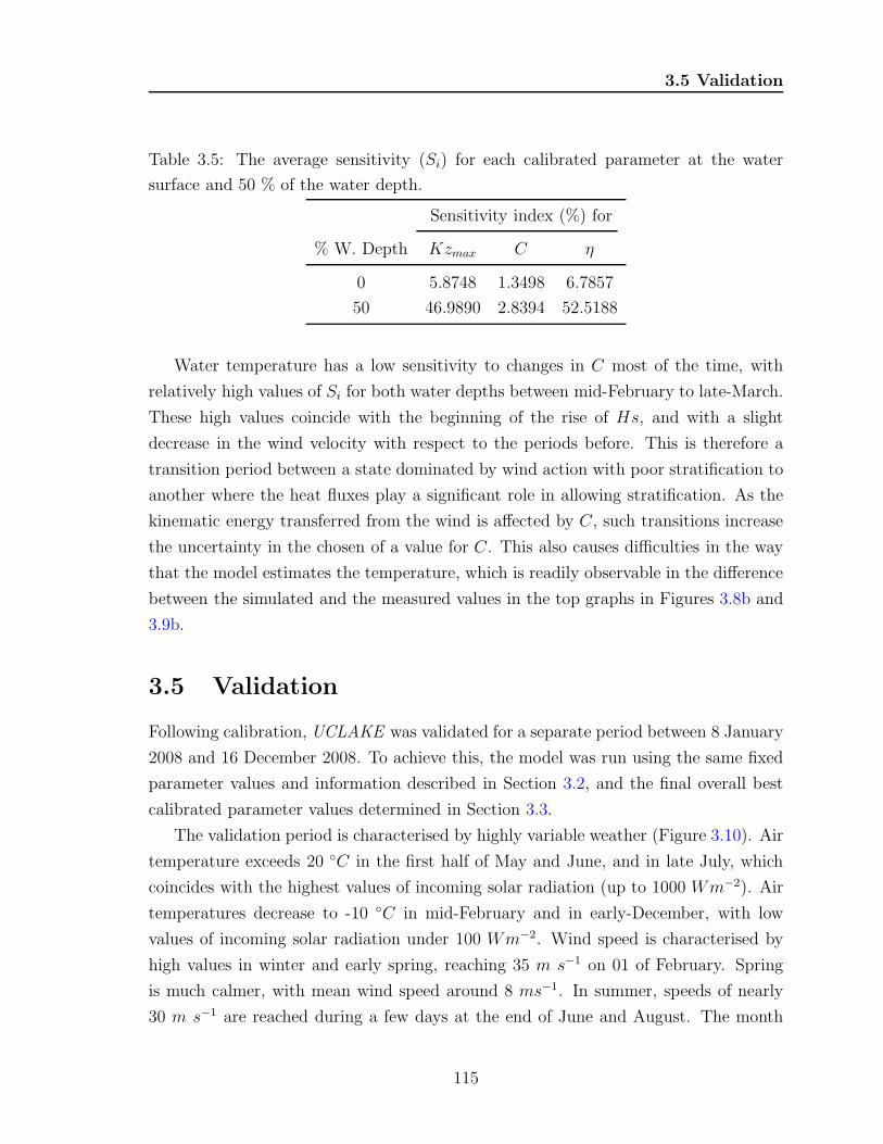
3.5 Validation
Table 3.5: The average sensitivity (Si) for each calibrated parameter at the water
surface and 50 % of the water depth.
Sensitivity index (%) for
% W. Depth Kzmax C η
0 5.8748 1.3498 6.7857
50 46.9890 2.8394 52.5188
Water temperature has a low sensitivity to changes in C most of the time, with
relatively high values of Si for both water depths between mid-February to late-March.
These high values coincide with the beginning of the rise of Hs, and with a slight
decrease in the wind velocity with respect to the periods before. This is therefore a
transition period between a state dominated by wind action with poor stratification to
another where the heat fluxes play a significant role in allowing stratification. As the
kinematic energy transferred from the wind is affected by C, such transitions increase
the uncertainty in the chosen of a value for C. This also causes difficulties in the way
that the model estimates the temperature, which is readily observable in the difference
between the simulated and the measured values in the top graphs in Figures 3.8b and
3.9b.
3.5 Validation
Following calibration, UCLAKE was validated for a separate period between 8 January
2008 and 16 December 2008. To achieve this, the model was run using the same fixed
parameter values and information described in Section 3.2, and the final overall best
calibrated parameter values determined in Section 3.3.
The validation period is characterised by highly variable weather (Figure 3.10). Air
temperature exceeds 20 C in the first half of May and June, and in late July, which
coincides with the highest values of incoming solar radiation (up to 1000 Wm−2). Air
temperatures decrease to -10 C in mid-February and in early-December, with low
values of incoming solar radiation under 100 Wm−2. Wind speed is characterised by
high values in winter and early spring, reaching 35 m s−1 on 01 of February. Spring
is much calmer, with mean wind speed around 8 ms−1. In summer, speeds of nearly
30 m s−1 are reached during a few days at the end of June and August. The month
115

3.5 Validation
01-Dec 01-Jan 01-Feb 01-Mar 01-Apr 01-May 01-Jun 01-Jul 01-Aug 01-Sep 01-Oct
Tem
per
ature
(oC
)
(1)
4
6
8
10
12
14
16
18
20
DataBest Simul.Kzmax (m2s−1) range
19/11/2006 08/01/2007 27/02/2007 18/04/2007 07/06/2007 27/07/2007 15/09/2007
0
20
40
60
Time
Sen
siti
vity
(%) (2)
(a) Kz
01-Dec 01-Jan 01-Feb 01-Mar 01-Apr 01-May 01-Jun 01-Jul 01-Aug 01-Sep 01-Oct
Tem
per
ature
(oC
)
(1)
4
6
8
10
12
14
16
18
DataBest Simul.C range
19/11/2006 08/01/2007 27/02/2007 18/04/2007 07/06/2007 27/07/2007 15/09/2007
0
5
10
15
Time
Sen
siti
vity
(%) (2)
(b) C
Figure 3.8: Sensitivity analysis of water temperatures at the water surface. 1) Compar-
ison of observed data, the best model simulation, and the range of model simulations
for the upper and the lower parameter limits. 2) Sensitivity index (Si) estimated using
Equation 3.2.
116

3.5 Validation
01-Dec 01-Jan 01-Feb 01-Mar 01-Apr 01-May 01-Jun 01-Jul 01-Aug 01-Sep 01-Oct
Tem
per
ature
(oC
)
(1)
4
6
8
10
12
14
16
18
20
DataBest Simul.η (m−1) range
19/11/2006 08/01/2007 27/02/2007 18/04/2007 07/06/2007 27/07/2007 15/09/2007
0
20
40
60
Time
Sen
siti
vity
(%) (2)
(c) η
Figure 3.8: Continued.
of February exhibits conditions similar to these encountered in the calibration period.
The air temperature decreases to -10 C, wind speeds drop below 5 m s−1, and very
little rainfall occurs.
During the calibration of UCLAKE, parameter set values were established based on
the optimisation of the NSE statistics. Such values shown also in Table 3.4 were used
in the validation of UCLAKE. These parameter set values were: Kzmax = 8.90×10⁻⁵,
C = 0.2 and η = 2.0.
Figure 3.11 shows a good agreement between the observed and the simulated tem-
perature, with NSE values of 0.9510, 0.9718 and 0.9725 at the water surface, mid-depth
and at the bottom respectively. Similarly, the temperature profiles at different times
(Figure 3.12), demonstrate the ability of the model to represent the temperature profile
at any time during the year. A maximum difference of 3.9 C during the first half of
February is registered and the mean RMAE is 8.1% for the 24 profiles plotted. Nu-
merical analysis of the vertical temperature structure throughout the validation period,
shows that RMAE is below 10% for 77% of the time. This confirms that the model is
able to simulate the whole vertical structure within the water column.
The main differences between simulated and observed series occur during the months
117

3.5 Validation
01-Dec 01-Jan 01-Feb 01-Mar 01-Apr 01-May 01-Jun 01-Jul 01-Aug 01-Sep 01-Oct
Tem
per
ature
(oC
)
(1)
4
6
8
10
12
14
DataBest Simul.Kzmax (m2s−1) range
19/11/2006 08/01/2007 27/02/2007 18/04/2007 07/06/2007 27/07/2007 15/09/2007
0
20
40
60
Time
Sen
siti
vity
(%) (2)
(a) Kz
01-Dec 01-Jan 01-Feb 01-Mar 01-Apr 01-May 01-Jun 01-Jul 01-Aug 01-Sep 01-Oct
Tem
per
ature
(oC
)
(1)
4
6
8
10
12
14
DataBest Simul.C range
19/11/2006 08/01/2007 27/02/2007 18/04/2007 07/06/2007 27/07/2007 15/09/2007
0
10
20
30
Time
Sen
siti
vity
(%) (2)
(b) C
Figure 3.9: Sensitivity analysis of water temperatures at 50% of the water depth.
1) Comparison of observed data, the best model simulation, and the range of model
simulations for the upper and the lower parameter limits. 2) Sensitivity index (Si)
estimated using Equation 3.2.
118

3.5 Validation
01-Dec 01-Jan 01-Feb 01-Mar 01-Apr 01-May 01-Jun 01-Jul 01-Aug 01-Sep 01-Oct
Tem
per
ature
(oC
)
(1)
4
6
8
10
12
14
16
DataBest Simul.η (m−1) range
19/11/2006 08/01/2007 27/02/2007 18/04/2007 07/06/2007 27/07/2007 15/09/2007
0
20
40
60
80
Time
Sen
siti
vity
(%) (2)
(c) η
Figure 3.9: Continued.
of February and March, where errors reach 50%. These discrepancies are caused mainly
by the time scale at which the model is implemented. Sub-daily changes in the meteo-
rological forcings are only weakly coupled to changes in the thermal structure because
the latter are gradual and usually lag the longer term weather conditions.
119

3.5 Validation
0
10
2001-Feb 01-Mar 01-Apr 01-May 01-Jun 01-Jul 01-Aug 01-Sep 01-Oct 01-Nov 01-Dec
Air
T.(o
C)
70
80
90
100
Rel
.H
um
i.(%
)
1020
1040
1060
1080
1100
Air
P.(m
bar)
0
5
10
Pre
ci.
(mm
/h)
10
20
30
Win
dV
.(m
/s)
12/02/2008 02/04/2008 22/05/2008 11/07/2008 30/08/2008 19/10/2008 08/12/2008
0
500
1000
Sol.
I.(W
/m
2)
Time (Hours)
Figure 3.10: Hourly meteorological variables between 08/01/2008 and 16/12/2008 used
during the validation of UCLAKE.
120

3.5 Validation
10
20
0% (Water surface)
1 2 3 4 5 6 7 8 9 10111213 14 1516 171819 20 21 22 23 24
DataSimulated
10
2010%
10
2020%
10
2030%
10
20
Tem
per
ature
(oC
)
40%
10
20
50%
10
20
60%
10
20
70%
10
20
80%
10
20
90%
12/02/2008 02/04/2008 22/05/2008 11/07/2008 30/08/2008 19/10/2008 08/12/2008
10
20
100% (Bottom)
Time
Figure 3.11: Comparison between the best simulated temperature (continuous line)
and the observed temperature (dashed line) at multiple water levels (every 20% of the
water depth from the water surface to the bottom). The vertical dashed lines indicate
the times of the profiles plotted in Figure 3.12.
121

3.5
Valid
atio
n
5 10 15 20500
505
510
515
520
W.dep
ht
(m)
1
5 10 15 20
2
5 10 15 20
3
5 10 15 20
4
5 10 15 20
5
5 10 15 20
Temperature (oC )
6
5 10 15 20
7
5 10 15 20
8
5 10 15 20
9
5 10 15 20
10
5 10 15 20
11
5 10 15 20
12
5 10 15 20500
505
510
515
520
W.dep
ht
(m)
13
5 10 15 20
14
5 10 15 20
15
5 10 15 20
16
5 10 15 20
17
5 10 15 20
Temperature (oC )
18
5 10 15 20
19
5 10 15 20
20
5 10 15 20
21
5 10 15 20
22
5 10 15 20
23
5 10 15 20
24
Figure 3.12: Observed (empty circles) and simulated (continuous line) water temperature profiles at different times
indicated in the Figure 3.11 (see numbers on the top right).
122

3.5 Validation
With the aim of testing the timestep scale issues, UCLAKE was set up using
daily averaged meteorological data, except for the solar irradiation where a single
value corresponding to the midday value was taken. The analysis shows that the
maximum temperature differences between observed and simulated decrease to 1.7 C
(50% less than in the analysis made using sub-daily time step data) with a decrease
in the RMAE to 6.1%. Although the analysis demonstrates that model performance
improves significantly when a daily timestep is used, the sub-daily details of the lake
stratification is not modelled and information on lake response to sub-daily variability
is lost.
Other sources of error are related to the uncertainty of the meteorological informa-
tion. Small changes in air temperature affect the temperature structure, especially the
mixed layer. Likewise, changes in wind forcing trigger changes in the flux of heat by
evaporation, and therefore changes in the net heat balance at the water surface. In-
cremental increase in wind speed can cause a misleading deepening of the mixed layer
and therefore changes in the temperature structure at the hypolimnion.
The high variability of the meteorological conditions at subdaily scales, where for
example wind speed varys from 0 to 40 m s−1 over the winter months, represents a
challenge to the modelling of the thermal structure in lakes at such scales, since the
numerical stability of the model is constantly affected. The condition of stability of
1D advection-diffusion models establishes that numerical calculations will be stable ifδ
2Kz∆t≤ 1 (Ryan & Harleman, 1973). Since Kz varies continuously, an adaption of ∆t
was required with the aim of guaranteeing numerical stability. Figure 3.13(a) shows
that ∆t usually varies between 0 < ∆t < 1405.5 s, and for some periods between
0 < ∆t < 3600 s. The analysis of frequency (see Figure 3.13 (b)) shows a two-mode
probability distribution function. The first mode indicates that values of ∆t close to 0
s are the most frequent (∼50% of the whole period), and correspond to the wind speeds
> 10 m s−1. The second mode indicates that ∆t around 1405.5 s are the second most
frequent and correspond to periods of thermal overturn. On the other hand, ∆t = 3600
s corresponds to wind speeds < 5 m s−1.
The relationship between wind speed and ∆t (see Figure 3.14) is inversely propor-
tional, so when wind speed increases the value of ∆t will decrease. A little dispersion is
shown in Figure 3.14. However, it is noticeable that ∆t = 1405.5 s is set independently
of the wind speeds when Kzmax reaches the threshold value 8.9 ×10⁻⁵ m2 s−1 which
corresponds to periods of thermal overturn. Since it is quite unusual in the literature to
123

3.6 Analysis of the Mixed Layer
02/04/2008 11/07/2008 19/10/2008
500
1000
1500
2000
2500
3000
3500
Time
∆t
(s)
(a)
1000 2000 30000
0.1
0.2
0.3
0.4
0.5
∆t (s)
Pro
bability
(b)
Figure 3.13: Analysis of the timestep (∆t) calculated by UCLAKE between 08/01/2008
and 16/12/2008 (validation period). a) ∆t against time; b) probability density function
of ∆t.
find lake dynamic models driven by wind speeds > 15 m s−1, the adaptive ∆t is a very
useful feature that makes UCLAKE extremely well suited to modelling the long-term
thermal structure of lakes subjected to strong wind forcing conditions. The adaptation
of ∆t in UCLAKE not only guarantees its numerical estability but also improves the
model performance.
3.6 Analysis of the Mixed Layer
Meteorological forcings are clearly the main factor driving the hydrodynamics of Llyn
Conwy. The wind velocity field interacts with the water body, triggering a near constant
stirring of the water column through the year (Figure 3.15 (c)). On the other hand,
increasing heat energy, especially in May, June and July, ensures certain periods of
continuous stratification (Figure 3.15 (b)), which are intermittently interrupted by the
occurrence of high wind speeds.
In winter and autumn, the lake is well mixed around 67.5 % of the time (Fig-
ure 3.16). The mean low incoming solar radiation and high wind velocities (mean 12.7
m s−1) ensure that the water column remains totally mixed. During early spring, the
lower average wind velocity of 11 m s−1 allows the lake to stratify for 44 % of the time
(Figure 3.16). The low temperatures and the high wind velocities, especially in the first
124

3.6 Analysis of the Mixed Layer
5 10 15 20 25 30 35
500
1000
1500
2000
2500
3000
3500
∆t
(s)
Wind vel. (m/s)
Figure 3.14: Relationship between wind speed and timestep (∆t) for the period
08/01/2008 to 16/12/2008.
half of March, guarantee a mixed layer through the whole month, with very episodic
overturns in the middle of the month. April is characterised by intermittent overturns
of the thermal structure due to the chaotic variance of the wind speed and the onset of
a more sustained air temperature rise. Through late April and May, the lake becomes
stratified with an apparently constant mixed layer depth of 2.5 m. This lasts through
the first half of May until an increase in wind speed above 12 m s−1 deepens the mixed
layer to 15 m.
As expected, the lake is stratified for about 80% of the time in summer (Figure 3.15
(b) and Figure 3.16). The mixed layer is held constant at 2 m and reaches the bottom
in the second half of June; stratification returns at the end of the month when the
wind forcing decreases from 30 ms−1 to below 10 ms−1. Periods of stratification occur
again in May and June, and episodic mixing due to wind forcing in late May, late June,
through July and August (Figure 3.15 (c)). The first half of July is characterised by
intermittent periods of stratification. However, the reduction in the wind speed and the
rise in air temperature over 22 C stimulates a rapid stratification that lasts until the
first week of August. Intermittent water mixing events through August are matched
by highly variable wind forcing that enhances mixing as the heat energy sources begin
to decrease.
125

3.6 Analysis of the Mixed Layer
0
10
20
Air
Te.
(oC
)(a)
01-Feb 01-Mar 01-Apr 01-May 01-Jun 01-Jul 01-Aug 01-Sep 01-Oct 01-Nov 01-Dec
10
20
30
Win
dV
e.(m
s−
1)
4
4
6
6
8
8
10
10
12
12
4
4
14
14
4
4
14
14
12
44
10
10
66
12
44
14
666
6
14
16
14 1412 1
214 1
4
6
44
44
14
812 1
4
18
8
44
10 6
14
14
12
10
6
16
141
4
14
14
14
16
14
14
14 18
18 14161
6 16 141
4
1814
146
(b)
W.D
epth
(m)
0
5
10
15
20
18/02/2008 31/03/2008 12/05/2008 22/06/2008 03/08/2008 14/09/2008 25/10/2008 06/12/2008
0
5
10
15
20
(c)
Time
Mix
.L
ay.
Dep
th(m
)
Mixed layer
Figure 3.15: a) Time series for dominant meteorological forcing variables air temper-
ature (black) and wind velocity (blue); b) simulated water temperature contours; c)
simulated mixed layer depth.
Figure 3.17 shows a complementary analysis of the lake stratification based on an
analysis of the energy balance. During the months of January, February and March,
the balance of energy at the water column is dominated by the wind kinematic energy
where no resisting forces, represented by the stratification gradient, appear to damp
the wind effects. Thus the whole range of wind magnitudes guarantee the homogeneous
temperature structure in the lake. Between the months of April and September, an
increase in incoming heat energy ensures stratification, raising the potential energy in
the lake and impeding wind stirring of the water column. It is also notable that, for
these months, wind velocities under 10 ms−1 (Figure 3.17 (b)) guarantee the existence
of the thermocline and the multiple mixing events are due to the gradual increase
126

3.6 Analysis of the Mixed Layer
Jan−08 Feb−08 Mar−08 Apr−08 May−08 Jun−08 Jul−08 Aug−08 Sep−08 Oct−08 Nov−08 Dec−08
0
20
40
60
80
100
Month
%oftime
Stratified Destratified
Figure 3.16: Relative duration of thermal stratification and destratification by month.
of the wind velocity over this threshold and the deepening of the mixed layer. In
winter, overturn of the water column is the predominant state. Stratification occurs
during short periods when wind speed falls below 5 ms−1 and the incoming solar
radiation provides sufficient heat energy to the uppermost layers. Winter is therefore
characterized by homothermal conditions controlled by high wind speeds that also
presumably serve to enhance turbidity by sediment resuspension.
127

3.6 Analysis of the Mixed Layer
0.5
1
1.5
2
2.5x 10
7
KE
(Nm)
(a)01-Feb 01-Mar 01-Apr 01-May 01-Jun 01-Jul 01-Aug 01-Sep 01-Oct 01-Nov 01-Dec
0
2
4
6
8
x 106
PE
(Nm)
(b)
12/02/2008 02/04/2008 22/05/2008 11/07/2008 30/08/2008 19/10/2008 08/12/2008
0
10
20
x 106
KE
-PE
(Nm)
(c)
Figure 3.17: (a) Wind kinematic energy (KE). (b) Mixed layer potential energy (PE).
(c) Net energy (KE - PE) available to stir the water column.
128

Chapter 4
FVCOM Graphical User Interface
(GUI) Development
Resume
A Graphical User Interface (GUI) to pre-process and post-process FVCOMinformation has been designed and programmed. The GUI is used to create theinput files required by FVCOM for different setups and to analyse and visualizethe results produced. It is specially configured for lake modelling problems. Thischapter begins with a description of the FVCOM input file configuration and abrief explanation of the different functions that these perform. The architectureof the pre- and post-processing interface is explained with the aim of giving anidea of its capabilities and some areas for future development. In order todemonstrate the use of the GUI, an illustrative case study of Llyn Cowlyd,North Wales, is set up using FVCOM-GUI.
4.1 Design Requirements of a GUI for FVCOM
4.1.1 Overview
Computational modelling requires interfaces to manipulate the model information in
an optimal and versatile manner. This is particularly the case for spatially-distributed
hydrodynamic models applied to environmental problems involving complex domain
boundaries (French & Clifford, 2000; Covelli et al., 2002). Most numerical model
129

4.1 Design Requirements of a GUI for FVCOM
codes require multiple data files that specify the computational mesh, bathymetry, and
boundary conditions. Additionally, one or more steering files are commonly required
to control aspects of model execution, including timestep, values for model constants,
and numerical solver parameter values. Dynamic simulations performed at high spatial
and temporal resolution generate large solution files and effective visualisation tools are
also required. Powerful pre- and post-processing software thus not only facilities and
simplifies the modelling process, but also allows the modeller to obtain greater insight
into the environmental problem being studied (Garcia-Martinez & Rodriguez-Molina,
1998).
Graphical User Interfaces (GUI) are increasingly provided as an integral part of
hydraulic and hydrological model codes. Commercial models such as the Mike series
(Havnø et al., 1995; Thompson et al., 2004) and Delft3D are packaged with GUIs that
offer comprehensive pre- and post-processing functionality. Other standalone software
packages, such as the Surface Water Modeling System (SMS, Zundel, 2005) offer similar
functionality in a generic format such that a broad suite of different model codes
are supported. Proprietary GUI software is typically programmed using a low level
language, often one with object oriented facilities such as Visual Basic, C++ and Java.
Such GUI software is often tied to a particular computer operating system, even though
many model codes are open source and capable of installation and compilation across
multiple platforms. However, such packages usually provide very powerful visualisation
features, such as the ability to overlay hydrodynamic solutions on base maps or to
generate animations.
Open source model codes originating from the research community tend to have less
well developed pre- and post-processing software. Sometimes, such GUI functionality
is provided in the forms of libraries of routines developed using scripting languages
such as Matlab or Python. For example, Rusu et al., 2008 describe the implementation
of a Matlab-based GUI for the SWAN shallow water wave model. From a research
perspective, development of GUIs using scripting languages offers greater flexibility
since the underlying code can be readily modified to suit particular user needs, even
where the scripting language itself is part of a proprietary package (such as Matlab
or IDL). Indeed, commercial packages such as Matlab are quite attractive for GUI
development on account of their in-built features that support specialised data storage
formats used within the modelling community (e.g. NetCDF ; Rew et al., 1997, Rew &
Davis, 2002), and tools for GUI programming (such as the GUIDE toolbox included
130

4.1 Design Requirements of a GUI for FVCOM
with Matlab). They also allow development of plotting, data extraction and video
animation capabilities to match any commercial package. Of course, the use of such
GUIs requires the user to have access to the scripting language, which generally requires
the purchase of the appropriate licence.
The FVCOM hydrodynamic code selected for the present study is not equipped
with a dedicated general purpose GUI. Accordingly, a major component of the study
has been the development of a GUI to provide a flexible and fast tool for the manage-
ment of FVCOM modelling tasks. As shown in Figure 4.1, the GUI includes both pre-
and post-processing tools. The pre-processing interface allows the user to set up the
input files that contain the model bathymetry, boundary conditions, initial conditions
and meteorological forcing data. The post-processing interface has been designed to
visualise and selectively analyse the solution files resulting from FVCOM model runs.
In particular, time series and vertical profiles can be derived for multiple variables at
a specific mesh node, and 2D plots can be produced for levels within the water column
or along a user-defined section. In addition, the post-processing interface includes an
option to produce and save animations to show the time evolution of any given variable.
FVCOM-GUI has been developed in Matlab. Matlab was selected as a development
platform for several reasons. First, it provides a powerful fourth-generation program-
ming language that incorporates a large set of built-in mathematical and data ma-
nipulation functions. Second, it has excellent graphical and visualisation capabilities.
Third, it includes a set of GUI design environment (GUIDE ) tools that allow interac-
tive creation of complex GUI templates. Fourth, specialised toolboxes are available to
perform functions that are crucial to supporting numerical hydrodynamic modelling
applications. Of particular importance, it the availability of a NetCDF toolbox that
greatly simplifies handling of the large (> 1Gb) model solution files produced by FV-
COM. Fifth, it is supported under most major operating systems (Linux, Mac OS X,
Windows). Finally, although it is proprietary product, Matlab is widely used within
the hydrodynamic modelling community and generally available within universities and
research institutes.
4.1.2 Structure of FVCOM Input and Result files
FVCOM requires a set of input files that vary according to the application. These are
all ascii text files. The model may write files in ascii format but the netCDF (Network
Common Data Form) format is more commonly specified for practical applications.
131

4.1 Design Requirements of a GUI for FVCOM
FVCOM
a)
b )
Figure 4.1: Schematic representation of the interaction of a) FVCOM-GUI pre-
processing and, b) post-processing with FVCOM.
132

4.1 Design Requirements of a GUI for FVCOM
NetCDF is distributed as a machine-independent software library that provides mul-
tiple functions to create, access and share scientific information. Its implementation
provides a format for representing scientific data in a compact and organised manner
(Rew & Davis, 2002). The netCDF format is widely used in climatology, oceanog-
raphy and GIS applications and offers an efficient means of storing and interrogating
very large multivariate data sets.
Overall execution of FVCOM is controlled by the casename run.dat file. This
includes information on the simulation duration and timestep, parameters that control
input and output (including format of the data fields), and certain global parameters
relating to diffusivity, baroclinic pressure gradient terms, and atmospheric and/or tidal
forcing. Other aspects of the computation, such as the representation of wetting and
drying, are governed by settings contained in this file. In addition to the run control
file, FVCOM requires a variable set of input files, which can be broadly classified
according to their function (Figure 4.2). These file groups include:
• INPUT FILES REQUIRED FOR ALL SETUPS : This is a group of manda-
tory files that contain essential information relating to the computational mesh,
bathymetry and boundary conditions.
• STARTUP DEPENDENT FILES : This group includes the files that define the
initial conditions depending on the RESTART option set in casename run.dat
file. A model can be cold-started from unknown initial conditions and spun-
up until it reaches a steady-state condition. Alternatively, a hot-start option is
available to enable the model to be restarted from a file containing all the model
variables saved from a previous simulation. This last option is useful for very long
simulations where, in some cases, it is necessary to stop and restart the model.
• METEOROLOGICAL FORCING DEPENDENT FILES : This file group con-
tains information on meteorological forcings. These can be spatially uniform
across the model domain and either time-varying or constant, or else can be spa-
tially varied (controlled by settings contained in the casename run.dat steering
file). Whilst many climate forcings are appropriately defined as time series dis-
tributed uniformly in space, there may be certain cases where spatially distributed
forcings may be required.
133

4.1 Design Requirements of a GUI for FVCOM
• OPEN BOUNDARY CONDITIONS SPECIFICATION FILES : This group of
files is used to define the open boundary conditions, including inflow and/or
outflow discharges and also, if required, water temperature and salinity.
• OPEN BOUNDARY SURFACE ELEVATION SPECIFICATION FILES : This
group of files is used to define time-dependent forcing of water surface elevation.
Although not relevant to lake simulations, various options are available to specify
tidal forcings.
• LAGRANGIAN TRACKING DEPENDENT FILES : This group includes only
one file that is used to specify the starting locations of particles tracked using
FVCOM’s Lagrangian tracking module.
• SEDIMENT MODELLING DEPENDENT FILES : These files are used to define
the physical characteristics of sediments and the structure and composition of
the bed, which can be represented as a series of layers. The sediment model may
optionally be forced by imposed suspended sediment concentrations at a set of
open boundary nodes or as point sources at river boundary nodes.
The outputs arising from an FVCOM model run can be obtained directly from
the screen during run-time execution. In practice, however, they are retrieved from
one or more NetCDF output files. The file casename 0001.nc, contains the mesh
configuration, bathymetry, and the values of the variables (previously specified in the
casename run.dat file) at every mesh node (or, for some variables, at the element
centres) for each time step.
The file casename ave 0001.nc contains the mean value of the selected variables
at specific time intervals. The file casename lag.nc is optionally used to save the
x, y and z coordinates of each particle followed by the Langrangian tracking module
through time. It is also possible to append the values of variables (e.g. velocity and
temperature) to each particle at every position.
It is evident from this brief overview of FVCOM input and output files that a
considerable effort is required to assemble and format the required information and
to organise the file set. This task also requires low-level understanding of FVCOM
file structures, source code organisation, and output formats - especially the NetCDF
file structure. This stage of the modelling process is therefore a prime candidate for
simplification by use of a GUI.
134

4.1 Design Requirements of a GUI for FVCOM
Casename_bfw.da t
Casename_c o r .da t
Casename_dep .da t
Casename_el_obc.dat
Casename_el j_obc.dat
Casename_el_ in i .dat
Casename_g r d .da t
Casename_h fx .da t
Casename_ i ts .da t
Casename_ jmpobc .da t Casename_lag_ in i .da tCasename_mc .da t
Casename_obc .da t
Casename_r iv . da t
Casename_spg .da t
Casename_uv_ in i .da t
Casename_wnd .da t
Casename_tsobc .da t
Casename_mean f low .da t
REQUIERED INPUT FILESFOR ALL SETUPS
RESTART = cold_start
Casename_r es ta r t .da t *
Casename_ i ts .da t
Casename_r es ta r t .da t *
M_TYPE = uniform
M_TYPE = non-uniform
S_TYPE = non-julian
S_TYPE = julian
OPEN B O U N D A R Y SURFACE E L E V A T I O N
S P E C I F I C A T I O N FILES
OPEN B O U N D A R Y CONDITIONS
S P E C I F I C A T I O N FILES
in i t_sed.F**
Casename_sed imen t . i np
Casename_sed_nudge.da t
Casename_sed_ptsource .da t
SEDIMENT MODELLING DEPENDENT FILESLAGRANGIAN TRACKING DEPENDENT FILES
METEOROLOGICAL F O R C I N G DEPENDENT FILES
S T A R T U P DEPENDENT FILES
Casename_run .da t
RESTART = hot_start
RESTART = hot_start_s
SED_PTSOURCE = T
SED_NUDGE = T
LAG_ON = T
FLAG_24 = -DSEDIMENT
FVCOM E x e c u t a b l e:
fvcom
S c r een r e p o r t
INFOFILE = screen CDF_OUT = T
Casename_0001 .nc
Casename_ave_0001.nc
Casename_ave_000n.nc
.
.
.
CDF_OUT_AVE = T
NetCDF output f i les Lagrang ian t rack ing ou tpu t f i l es
LAG_ON = T
Casename_lag .nc
. /FVCOM2.6.1/ run/
. /FVCOM2.6 .1 /mode ls /casename/
. /FVCOM2.6.1/ run/OUTDIR_casename/
. /FVCOM2.6.1/FVCOM_source/I n p u t F i l e s
O u t p u t F i l e s
R u n t i m e C o n t r o l P a r a m e t e r s F i l e
Notes :1) * F i l e s dumped by FVCOM in ear ly s imula t ions2) ** FVCOM source f i les located in: . /FVCOM2.6.1/FVCOM_s o u r c e/3) Uncomment f lag in the FVCOM m a k e f i l e
Figure 4.2: Structure of input and output files in FVCOM.
135

4.2 GUI Architecture
4.2 GUI Architecture
The overall GUI architecture is summarised in Figure 4.3. The GUI starts by ex-
ecuting a Matlab script fvcom gui.m, which calls the two main program modules,
sms2fvcom.m and main.m, that manage the pre-processing and post-processing inter-
faces respectively.
aux_functions post-processing
FVCOM-UCL-GUI(v1.0)
fvcom_gui.m/fig ucl.jpg pre-processing
Figure 4.3: FVCOM-GUI file and directory structure.
The pre-processing functionality is provided by a set of Matlab script files contained
in the pre-processing directory. These are invoked as required by the managing script
sms2fvcom.m , as shown in Figure 4.4. The pre-processing is described by the flow
chart represented in Figure 4.5. Pre-processing starts with the reading of two files
that contain the x and y coordinates of the computational mesh, and the x and y
coordinates of the boundary nodes. Generation of the computational mesh is thus
handled externally (the Surfacewater Modeling System, SMS, has been used to generate
all the mesh files used in this study) and this functionality is not presently built into
the GUI. Once these files have been read, the mesh can be displayed.
The GUI then allows the user to set three kinds of boundary conditions (BCs): solid
boundaries, specified inflows and outflows, and open boundary conditions (OBC). At
solid boundaries it is assumed that there is no flow through the boundary and this
is the default boundary type within FVCOM. Alternatively, inflows can be defined
as point sources where discharge, temperature and/or salinity can be set for a specific
mesh boundary point and elevation for groundwater inflows, or else distributed through
the water depth in the case of river inflows. Outflows are specified in the same way
but signed as negative values. The OBC option, includes ten distinct types of open
boundary conditions used to model forcing by time-varying water surface elevations.
These include a range of tidal options and are not fully implemented in the present
version of the GUI (they are not immediately relevant to lake modelling problems).
136

4.2 GUI Architecture
aux_functions
fvcom_gui.m/fig
ucl.jpg
FVCOMinput_files.m/fig
meshpatch.m
meshpoints.fig
nearest_oi_node.m
sms2fvcom_settings.mat
pad.m
sms2fvcom.m/fig
bathy_plot.m
check_point_level.m
check_plan_level.m
check_point.m
check_points_dist.m
check_time.m
element_surro_node.m
interp.m
mesh_plot.m
myupdatefcn1.m
open_netcdf_file.m
plot_figure1.m
plot_figure2.m
plot_figure3.m
plot_figure4.m
plot_figure5.m
plot_patch.m
point_level.mpreliminary_netcdf_datas.m
savePlotWithinGUI.m
spatial_level.m
xys_coordinate.m/fig
sms2fvcom.m/fig
main.m/fig
1
2
3
4
5
2, 6
6
7
8
7
5
main.m/fig
pre-processing post-processing
BASIC ROUTINES
save_fig.m
2, 6
1, 6, 8
3, 4, 5, 6
Figure 4.4: FVCOM-GUI script file dependencies. The BASIC ROUTINES are scripts
called on multiple occasions by the post-processing routines.
137

4.2 GUI Architecture
BC assignment is handled interactively. The user first specifies a BC type and
then selects the associated boundary points on screen. For each node selected in this
way, the GUI records, the type of BC, the node number and its x and y coordinates.
Multiple BC types can be set for a study case, by repeating the selection of BC, the
points chosen and the saving of the information.
The GUI is presently configured to generate the various categories of FVCOM input
file as described in Section 4.1.2. At the present time, however, generation of the OPEN
BOUNDARY CONDITIONS SPECIFICATION FILES is not fully implemented. The
GUI will always write the first file group, REQUIRED INPUT FILES FOR ALL
SETUPS, and will write other files according to options chosen by the user. The GUI
pre-processing stage can be exited after the necessary input files needed have been
written. Multiple model setups are possible without having to exit the GUI, which is
convenient for the preparation of a set of model runs with varied parameters or forcings.
The post-processing module of the GUI is designed to visualise and analyse the
information contained in FVCOM solution files. The program flow is summarised
in Figure 4.6. The first stage involves selection and opening for read access of an
FVCOM -generated NetCDF file (see **NetCDF file (Mod.) in Figure 4.6). Several
additional options are available here. These include options to read a netCDF file
containing relevant observational data in a compact format; a NetCDF file containing
information from a particle tracking simulation; and/or the meteorological forcing data
file casename mc.dat which is used as one of the input files for an FVCOM model run.
These optional files facilitate comparison between model predictions and observations,
and also allow convenient visualisation of the relationship between modelled outcomes
and the main (in this case meteorological) forcings used in the model run.
Once the NetCDF data files are read, the GUI invites the user to select from various
visualisation options:
• 1D analysis (One variable): This option allows the user to plot either the
time evolution or the variation with depth of a variable, at one or more locations
within the model domain (selection of up to five locations is currently supported).
The time evolution and the depth variation plots differ from each other in that,
in the case of the former the user must specify the start and end time, whereas for
the latter only a single time is required. The x, y and z (σ level) coordinates of
the points chosen can be set interactively by selecting points in the mesh. At this
138

4.2 GUI Architecture
Start
Read**x y mesh node coor.
Read** x y bound. mesh node coor.
Select boundary type?
Optional files
Conventions:
Set:casename
latitude
Write FVCOM files:
-REQUIRED INPUT
FILES FOR ALL SETUP
Advance setup?
End
STARTUP DEPENDENT FILES
METEOROLOGICAL FORCINGDEPENDET FILES
OPEN BOUNDARY CONDITIONS
SPECIFICATION FILES
OPEN BOUNDARY SURFACE
ELEVATION SPECIFICATION FILES
LAGRANGIAN TRACKING
DEPENDENT FILES
SEDIMENT MODELLING
DEPENDENT FILES
Inflows and outfows Open boundary conditions
(Tidal / water level coditions)
Yes
No
Yes
No
(Assu
me
solid
B.C
.)
Figure 4.5: Pre-processing FVCOM-GUI flow diagram.
139

4.2 GUI Architecture
Start
Read**NetCDF file (Mod.)
Read**NetCDF file (Obser.)
ReadParticle Track. file
ReadMeteo. forcing file
Type of analysis
1D Analysis (One var.) 2D Analysis (XY view)1D Analysis (Two var.) 3D Analysis (Under constr.)2D Analysis (Cross section)
Ask for:
- Dimension
- Variable
- Time in
- Time out
- Numb. of points
- x y coordinates
- Include ext. files
Ask for:
- Dimension
- Variable 1
- Time in
- Time out
- Numb. of points
- x y coordinates
- Variable 2
- Variable
- Time
- Level
- Kind of plot
- Include ext. files
Ask for:
- Variable
- Time
- Kind of plot
Ask for:
Visualization mode
DynamiclStatic
Plot picture
Save picture:
*.jpg *.png *.bmp *.eps
Set movie info.
Reproduce movie
Save movie
*.avi *.mov
End
Input files
Optional files
Conventions:
Figure 4.6: Post-processing FVCOM-GUI flow diagram.
140

4.2 GUI Architecture
stage there is also an option to plot meteorological forcing data and/or observed
variables along with the modelled information.
• 1D analysis (Two variables): This option allows the user to plot two dif-
ferent variables through time or the water depth in the same axes for an specific
point, with the aim of comparing both series.
• 2D analysis (XY view): This option is used to plot an XY view of a variable
for a specific time and level within the water column (σ level). This option offers
the possibility of plotting the information in any of the three following ways:
contours, filled contours and as a vector field. These plot types are enabled
for all the variables listed in a pop-up Variable menu, with the exception of
the vector field plot type, which is only available for the velocity variable. As
with the two 1D options described above, this option includes the possibility of
including a meteorological forcing variable for a specific time. There is a further
option to plot the positions of particles simulated using particle tracking features
in FVCOM.
• 2D analysis (Cross section): This option is used to plot the values of a
variable along a cross section (or transect) for an specific time. The cross section
is defined by entering the x, y and z coordinates for two points to define the start
and end points of a transect. An algorithm within the GUI firstly searches the
triangular elements that are intersected by the line, then projects perpendicularly
the vertices of the elements found onto the transect and calculates the new x
and y coordinates along the line; the σ coordinates are kept untouched. To
visualise information contained in the projected nodes, the algorithm transforms
the σ coordinates to real coordinates and interpolates the attribute (value of the
variable choosen) of each node onto a orthogonal rectangular grid adapted to
transect.
• 3D analysis: This option is still under construction but, when completed, will
allow plotting of results in three dimensions.
After the analysis type has been specified using one of the options described above,
the user is ready to visualise the information using either a Static or Dynamic
mode. The Static mode plots the information already defined for the chosen Type
of Analysis option. On the other hand, the Dynamic mode is used to produce
141

4.3 Example Application of GUI to Pre- and Post-process FVCOM
Simulation
Table 4.1: Geographical information for Llyn Cowlyd.
Location Snowdonia National Park, North Wales
Coordinates: 53o08′N 3o55′W
Altitude: 355.00 m
Maximum length: 2.78 km
Surface area: 1.1 km2
and save a movie animation, and this is available only for a sub-set of the Type of
Analysis options: 2D analysis (XY view), 2D analysis (Cross section) and
3D analysis. The user must set under the Dynamic label, the number of frames to be
recorded, the start time and the end time of the movie; the water level for the option
2D analysis (XY view) must be set in its own menu. Movie animations are saved
using the AVI format, and can replayed using any software that supports this format.
To save the AVI file, an algorithm divides the time interval by the number of frames
and sets a series of new times that are approximated to the nearest simulated times,
with the aim of retrieving the information from the NetCDF file for each time. The
files can also be played using the implay tool in Matlab, which offers multiple options
to play, pause, and step through an animation.
4.3 Example Application of GUI to Pre- and Post-
process FVCOM Simulation
In order to demonstrate further the functionality provided by the new FVCOM-GUI, a
hypothetical model set up for Llyn Cowlyd (Lake Cowlyd) is presented. This is another
small upland lake in North Wales, and provides a good illustration of the tasks involved
in implementing an FVCOM model and visualising the modelled hydrodynamic be-
haviour. Table 4.1 summarises the principal geographical and physical characteristics
of the lake. This demonstration FVCOM simulation is setup using null values for all
the meteorological forcing data included in the Cowlyd mc.dat file, with the exception
of the wind forcing, which was set up with a constant northerly wind of 10 m/s. The
properties of the computational mesh and the run control parameters are summarised
in Table 4.2.
142

4.3 Example Application of GUI to Pre- and Post-process FVCOM
Simulation
Table 4.2: Llyn Cowlyd FVCOM model setup information.
No. of Nodes 831
No. of Elements 1492
No. of layers 15
Mean length element edge: ≈ 32 m
Duration 15 days
∆t: 1 s
Installation of the GUI is straightforward. First, the user must obtain and uncom-
press the archive FVCOM-UCL-GUIv1.0.tar.gz. Next, Matlab must be started and its
path set to the FVCOM-UCL-GUIv1.0 directory path. The GUI has been tested un-
der linux (RedHat Enterprise Linux ), MacOS-X (10.6.8 Snow Leopard), and Windows
XP/Vista/7 operating systems with Matlab2008b or later pre-installed. To start the
GUI, the user must type fvcom gui at the Matlab command line. The FVCOM-GUI
start-up screen is then displayed (Figure 4.7).
At this stage, the user can choose between pre- and post-processing functionalities.
The GUI can also be exited at this stage. Pressing the pre-processing button, results
in the window shown in the Figure 4.8 being displayed. The Select new mesh file
button is used to open the SMS Llyn Cowlyd.2dm file that contains information
about the mesh configuration, and the Select new BC files button is used to open
the Llyn Cowlyd.bc file that identifies which nodes are located on the mesh boundary.
Both files are then read into memory using the Read files button.
Display of the computational mesh is toggled by the Show/Hide mesh button.
Boundary types are then selected interactively by stepping through the set of bound-
ary node segments specified in the BC input file. An undo option has been implemented
here so that any mistakes can be immediately rectified. For the purpose of this illus-
trative example, the lake is considered to be enclosed by a closed solid boundary (the
default option in FVCOM ).
Once the Casename and Latitude fields have been populated, the Write FVCOM
files button is used to write the minimal set of REQUIRED INPUT FILES FOR
ALL SETUP. This set of files is sufficient for this GUI test case. The FVCOM model
can now be executed.
Once FVCOM model execution has been finished successfully, the user can visualise
the results using the post-processing mode. On selecting the post-processing option
143

4.3 Example Application of GUI to Pre- and Post-process FVCOM
Simulation
Figure 4.7: FVCOM-GUI startup ’splash screen’ and menu to choose between pre- and
post processing modes.
(see Figure 4.7), the window shown in Figure 4.9 prompts the user to open a NetCDF
solution file. A filesystem browser dialogue filters files with a *.nc filename extension.
Once the NetCDF file is opened and read, the interface is transformed and new func-
tions become available, as is shown in the Figure 4.10. In this case, a file Cowlyd 0001.nc
generated by a previous FVCOM run has been selected. This window allows the user
to open and read additional files at any time during the post-processing usage. For
example, if the user wants to include the meteorological data use to force the model
run, they can check the square box under the Meteorological Forcing File frame
and a dialogue will be displayed to open the relevant file. A list of meteorological forc-
ing variables will then be displayed under the Meteo. Forcing Var. popup menu,
144

4.3 Example Application of GUI to Pre- and Post-process FVCOM
Simulation
Figure 4.8: Pre-processing window where the SMS files are read, and the required files
are created.
ready to be selected.
The Type of Analysis pop-up allows the user to select from the five different
modes of analysis outlined in Section 4.2. Each type of analysis has its own Input
Values frame, so each time the user changes the type of analysis a new frame will
appear underneath. In the current example, the 1D Analysis (One variable) op-
tion has been chosen. A temporal analysis has been selected here (the default) with
Velocity as the variable chosen using the Variable pop-up menu. Additionally, the
values of Time in and Time out must be set using either the manual entry field or
the slider. The user will notice that any value introduced in the manual entry field will
cause a movement in the slider. Likewise, the time indicated by the slider position will
automatically appear in the entry field. The user will also see that the time set under
Time in frame can not be greater than the one under Time out frame, so if the first
one is set greater than the second one both sliders are pulled back to the minimum
time.
For the 1D Analysis (One variable) option, it is also necessary to choose the
number of points at which to plot the variable chosen. Using the Number of points
145

4.3 Example Application of GUI to Pre- and Post-process FVCOM
Simulation
Figure 4.9: Post-processing window where the NetCDF file is read.
pop-up menu 5 points have been chosen (the maximum number of points available)
and the window shown in Figure 4.11 then appears. This allows the user to set the x
and y coordinates and the water level of the points interactively using the mouse or by
entering coordinates manually in the relevant fields. To select a point, the user has to
press its associated radio button (the small circular buttons) and then click on any node
on the mesh. Each time the user clicks on a node on the mesh, the x and y coordinates
fields are updated along with the lower (water surface level) and upper (bottom level)
limits of the Sigma-level slider. If the coordinates are already known, these can
be entered manually, and the interface will automatically find the nearest mesh node.
Once the points have been chosen, it is possible to save, then using the Plot button
to plot the points using numbered red spots (see Figure 4.11). Additionally, the Clear
plot remove the points plotted.
Once the information required for the 1D Analysis (One variable) option has
been set, the user is ready to plot the Variable from Time in to Time out at the
points already selected by pressing the Plot button. The time series are plotted within
the graphic pane on the right hand side of the window (see Figure 4.10). In the event
146

4.3 Example Application of GUI to Pre- and Post-process FVCOM
Simulation
Figure 4.10: Post-processing window showing the multiples files available to read, so
that the input information for the 1D Analysis (One variable) type of analysis.
that multiple points are specified, the plot lines are colour coded.
Vertical variation in a variable over the water depth can be plotted by selecting the
Water depth radio button under Kind of analysis and by setting the parameters
available under this option. Figure 4.12 shows plots of the x, y and z components of
the vector velocity and its magnitude, where each colour represent a different point.
Note that shorter velocity profiles correspond to shallower locations in the lake.
Further analysis can be chosen from the Type of Analysis pop-up menu. In Fig-
ure 4.13 the type 2D Analysis (XY view) has been chosen to represent the velocity
field, most of the options for which are set up in the way described above for the 1D
Analysis (One variable). The user will notice that the lower limit (water surface
level) of the Level slider will change according to the the time. Additionally, the user
can choose between three different kind of plots: contours, filled contours and
vector field. The user can either pick one or all three of these options using the
square check boxes placed in the Kind of plot frame.
Figure 4.13 shows a 2D Analysis (XY view) analysis in which the user has also
147

4.3 Example Application of GUI to Pre- and Post-process FVCOM
Simulation
Figure 4.11: Post-processing window to select points on the computational mesh.
Figure 4.12: Post-processing window with velocity components and magnitude plotted.
148

4.3 Example Application of GUI to Pre- and Post-process FVCOM
Simulation
Figure 4.13: Post-processing window with velocity field and wind forcing information
plotted.
149

4.3 Example Application of GUI to Pre- and Post-process FVCOM
Simulation
selected and read in the Meteorological Forcing File. The graphic pane thus dis-
plays both the velocity vector field, including filled contours for a particular moment
in time and a specified level. In addition, the wind forcing information (wind velocity
and direction) is plotted in a small set of axes placed in the left upper corner.
The 2D Analysis (Cross section) option is illustrated in Figures 4.14 and 4.15.
In contrast to the 2D Analysis (XY view), this option does not require the user to
specify a given water level, nor does this option support inclusion of external infor-
mation (such as meteorological forcing or particle tracks). Instead, the 2D Analysis
(Cross section) option requires a cross section of the basin to be defined by inter-
actively setting the x and y coordinates for its start and end points. Figure 4.14 shows
this process after the user has just entered the transect co-ordinates. Both points are
highlighted on the mesh and the transect line has been plotted. The velocity field for
the section shown in Figure 4.14 is plotted in Figure 4.15.
Figure 4.14: Post-processing window to define a cross section.
In conclusion, it should be noted that any plot displayed within the GUI can be
saved using the Save file button. In the case of a movie animation, the Dynamic frame
must be activated and the information required under it must be provided. As in the
pre-processing module, the GUI can be shutdown using the Close button.
150

4.3 Example Application of GUI to Pre- and Post-process FVCOM
Simulation
Figure 4.15: Post-processing window representing the field velocity in a cross section.
151

Chapter 5
3D Modelling of Wind-Driven
Circulation and Bottom Stress
Resume
This chapter applies the 3D FVCOM model to investigate various aspects ofthe hydrodynamics of Llyn Conwy. FVCOM is evaluated with respect to ver-tical velocity profiles measured by ADCP deployments in the second field cam-paign. This is complemented by an analysis of surface seiche and internal wavemotions, aided by observations of pressure and temperature fluctuation. Thesimplified wind wave model, UCL-SWM, is calibrated and validated againsttime-series of surface wave variables obtained at selected locations around thelake shore. A comprehensive analysis of wind records from 1993 to 2011 is un-dertaken to determine the characteristics of extreme wind forcing events andthe most prevalent wind directions. Multiple wind speed and wind directionscenarios along with water surface level scenarios are specified and the spaceand time variation in bottom stress due to the effects of wind-driven currentsand waves is investigated in detail. The chapter concludes with the analy-sis of bottom shear stresses during December 1997, which includes the highestmagnitude wind forcing event between 1993 and 2011.
5.1 Introduction
As shown in Chapter 4, one-dimensional hydrodynamic models can provide valuable
insights into the thermal evolution of lakes that are especially useful in characterising
152

5.1 Introduction
lake behaviour over seasonal and multi-annual timescales. However, such models ne-
glect aspects of the circulation that can be very important, even in small lakes, when
the externally-imposed wind stress is strong, or when inflows and outflows are signifi-
cant (e.g. Imberger & Hamblin, 1982, Hodges et al., 2000). In lakes subject to strong
wind forcing, horizontal gradients are no longer negligible and complex patterns of
circulation arise due to the interaction with bathymetry. These water movements may
exert a significant influence on the transport and deposition of sediments (Csanady,
1975) and knowledge of this aspect of lake hydrodynamic behaviour is thus very im-
portant to inform any subsequent analyses of lake depositional sequences (e.g. for
palaeoenvironmental reconstruction).
This chapter demonstrates the application of the 3D FVCOM model to investigate
various aspects of the hydrodynamics of Llyn Conwy. First, the ability of FVCOM
to resolve the vertical velocity profiles generated by wind-generated surface stress is
investigated with reference to the ADCP datasets obtained during the second field
campaign. This is complemented by an analysis of oscillatory motions, both surface
seiche effects and internal waves, aided by observations of high-frequency pressure fluc-
tuations from the first field campaign and the vertical thermistor chain data from the
CEH data buoy. Second, the space and time variation in bottom stress due to the
effects of wind-driven currents and waves, in isolation and in combination, is inves-
tigated. This involves calibration and validation of the simplified wind wave model,
UCL-SWM, against time-series of surface waves obtained at selected locations around
the lake shore during the second field campaign. In addition a comprehensive analysis
of wind records from 1993 to 2011 is undertaken to determine the characteristics of the
most extreme wind forcing events, and also the most prevalent wind directions. From
the wind forcing frequency analysis, multiple wind speed and wind direction scenarios
along with water surface level scenarios, are established with the aim of analysing the
effects of the wind forcing and water surface level changes on the bottom shear stress
distribution. The chapter concludes with the analysis of bottom shear stresses during
the month of December 1997, which is a period of strong winds and includes the high-
est magnitude wind forcing event between 1993 and 2011. This analysis informs the
subsequent analysis of the nature and controls on bottom sediment accumulation in
Chapter 6.
153

5.2 Calibration and Validation of FVCOM
Table 5.1: Set-up of FVCOM for calibration.
Parameter value
Starting date 03/04/2011 14:00:00
Finishing date 08/04/2011 07:00:00
# of elements 2028
# of nodes 1097
# of σ levels 12
∆t(s) 1.0
Mean element edge length (m) 13.2
5.2 Calibration and Validation of FVCOM
5.2.1 Calibration
Full calibration of 3D hydrodynamic models is not always undertaken because of the
high computational requirements. Many 3D models thus use parameter values obtained
from previous sensitivity analysis with simpler 1D and 2D models. Parameters such
as bottom roughness (z0) are established based on physical characteristics such as
sediment grain size and density. For example in Clear Lake California, USA, where
sediments are predominantly muddy, Rueda et al., 2003 set z0 = 0.02 cm to implement
a 2D model. In Lake Okeechobee Florida, USA, a relative high value of z0 = 0.5
cm was set to take account of abundant vegetation in littoral areas (Jin et al., 2000).
Other studies (e.g. Gross et al., 1999) suggest a spatial distribution of z0 based on the
local depth, to account for the effects of wave motions in the hydrodynamic model.
Despite an extensive literature on the roughness coefficient, its specification is often
rather arbitrary.
Here, a calibration with respect to z0 was carried out against the velocity profiles
recorded using an ADCP at location 1 (ADCP1) shown in Figure 2.14. z0 was assumed
to follow a uniform distribution between 0.001 m to 0.06 m (Ji, 2008), with values
sampled at random using a Monte-Carlo approach. Model performance was evaluated
following the performance functions described in Chapter 2, with particular emphasis
on the maximisation of the Nash-Sucliffe coefficient (NSE). The characteristics of the
model setup used for each simulation are summarised in Table 5.1.
154

5.2 Calibration and Validation of FVCOM
FVCOM was forced by the meteorological data recorded during the second field
campaign (Figure 5.1). The meteorological wind forcing series shows that, a south-
westerly wind is the dominant pattern (Figure 5.1b) with velocities fluctuating mainly
between 12 and 16 m s−1.
The initial conditions were established by spinning up the model over two days
using a constant wind speed (11.2 ms−1) and direction (241.92o) which correspond to
the wind forcing conditions at the start of the calibration period. To illustrate the
model performance during the spin-up time, the temporal evolution of the vertical
velocity structure is shown at two different points (Figure 5.2) chosen randomly in the
lake basin (see Figure 5.3 for the point locations). At both points, the velocity structure
behaves chaotically over the first two days because the water body is accelerated from a
static condition by the wind forcing. After the first day the flow becomes more stable,
and a more organised velocity structure is observed, but still with no steady structure
at P2 (Figure 5.2b). Only after the end of the two-day spin-up period, does the velocity
structure tends to be more stable.
The resulting flow velocity fields at the water surface (Figure 5.3a) and at the
mid water depth (Figure 5.3b) after the spin-up period, give preliminary clues about
the characteristic circulation patterns in the lake. A comparison between both shows
similar patterns of circulations especially at the northern and the eastern sides of the
lake. In these areas, the formation of an anticyclone gyre is visible after the confluence
of two strong current flows at the east of the lake. The first originates from the north,
and the second from the south centre of the lake.
Not only are initial conditions for the flow field required, but also scalar magnitudes
such as water temperature need to be defined at the initial time step. A uniform
distribution of the water temperature was set, equal to 4.71 oC based on the thermal
structure analysis described in Chapter 3. This showed that in the month of April, the
lake stays mixed more than 40% of the time and during intermittent stratified periods,
the thermocline is not significantly sharp.
Simulations were performed for 90 different values of z0, from which the best pa-
rameter was found by the maximisation of the NSE (Figure 5.4a). The results of the
calibration show a generally acceptable model performance (NSE > 0.5) for all the z0
values. Figure 5.4b shows that as the values of z0 grow between 0.001 and 0.02 m, NSE
increases rapidly, reaching its maximum value of 0.84 when z0 = 0.0227 m. Then, NSE
155

5.2 Calibration and Validation of FVCOM
180200220240260280
Winddir.(o)
5
10
15
Windvel.(m
s−1)
04 00 04 12 05 00 05 12 06 00 06 12 07 00 07 12 08 00
0
200
400
600
(Wm
−2)
Time (Day and hour)
HsHn
(a)
10%
20%
30%
40%
WEST EAST
SOUTH
NORTH
0 - 2
2 - 4
4 - 6
6 - 8
8 - 10
10 - 12
12 - 14
14 - 16
16 - 18
18 - 20
(b)
Figure 5.1: Hourly meteorological forcing from 03/04/2011 to 08/04/2011. a) Wind
direction, wind speed measured 10 m above the ground and, incoming solar radiation
(Hs) and net heat flux (Hn). b) Wind rose where the colour scale and the concentric
circles indicate the wind speed (m s−1) frequency.
156

5.2 Calibration and Validation of FVCOM
0.0
1
0.01
0.0
1
0.0
1
0.0
2
0.0
2
0.0
2
0.0
2
0.0
2
0.02
0.0
3
0.03 0.03 0.03 0.03
0.0
3
0.03
0.0
4
0.04
0.0
4
0.05
0.0
5
0.0
6
0.0
6
0.0
7
Time (sec)
W.D
epth
(m)
0 2 4 6 8 10 12 14 16
x 104
−20
−15
−10
−5
(a)
0.0
10.0
20.0
20.0
30.0
30.0
40. 0
40.0
50. 0
5
0.05
0.0
60.0
6
0.06 0.06 0.06 0.06
0.0
6
0. 0
6
0.0
7
0.0
7
0.0
7
0.0
7
0.07
0.0
7
0.07 0.07 0.07
0.0
7
0.0
7
0.0
7
0.070.070.07
0.07 0.07 0.07
0.07
0.0
8
0.08
0.0
8
0.080.080.08
0.08
0.08 0.08 0.08
0.0
8
0. 0
80.0
9
0.09
Time (sec)
W.D
epth
(m)
0 2 4 6 8 10 12 14 16
x 104
−6
−5
−4
−3
−2
−1
(b)
Figure 5.2: FVCOM model spin-up of the flow velocity structure at two different points
during 2 days of simulation time. a) Magnitude of flow velocity at P1; and b) at P2.
The locations of the points are shown in Figure 5.3.
function decreases slightly to ∼0.80 for z0 > 0.0227 m, indicating model insensitivity
for that set of z0 values.
Additional model performance analysis yields a correlation coefficient of ∼0.9 be-
tween the wind speed and the depth-averaged observed and best simulated flow velocity
series. This shows that both the lake and the model are thus very sensitive to changes of
wind speed and respond quickly to wind forcing changes despite the relative shortness
of the meteorological data time step (1 hour).
Although the model performs well for the best z0 values, it underestimates the flow
speed by almost 25% at the velocity peak that occurred around 6 am on 5 of April.
In contrast, model overestimation occurs around 6 am on 04 of April and is even more
157

5.2 Calibration and Validation of FVCOM
2.777 2.778 2.779 2.78 2.781 2.782 2.783 2.784
x 105
3.457
3.458
3.459
3.46
3.461
3.462
3.463
3.464
3.465
x 105
0 m s−1
0.19 m s−1
Velocity scales Wind V. = 11.2 m s−1
P1
P2
East (m)
Nort
h(m
)
Flo
wsp
eed(m
s−
1)
0.04
0.06
0.08
0.1
0.12
0.14
0.16
0.18
(a)
2.777 2.778 2.779 2.78 2.781 2.782 2.783 2.784
x 105
3.457
3.458
3.459
3.46
3.461
3.462
3.463
3.464
3.465
x 105
0 m s−1
0.19 m s−1
Velocity scales Wind V. = 11.2 m s−1
P1
P2
East (m)
Nort
h(m
)
Flo
wsp
eed(m
s−
1)
0.02
0.04
0.06
0.08
0.1
0.12
0.14
0.16
0.18
(b)
Figure 5.3: Initial conditions of the water velocity field at a) surface layer and b) mid
layer for FVCOM model on 03/04/2011 at 2 pm.
significant at the end of the period when overestimation is nearly 30% when the flow
is relatively low. Such discrepancies are also visible in the sensitivity analysis of z0
(Figure 5.5). Observing Figure 5.5 (b), it is evident that the sensitivity index varies
through time, so it may be eventually possible to obtain not only a unique value for z0
but different ones for different periods. The sensitivity index shows also that the model
is relatively sensitive (> 30%) to changes of z0 when flow velocities are greater than
0.05 m s−1, and less sensitive (< 20%) when flow velocities are lower. The behaviour
of the sensitivity index suggest that the model performance would be improved if z0
were ≤ 0.005 m for relatively high flow velocities and ≥ 0.01 m for lower velocities.
5.2.2 Validation
Validation was carried out against the velocity profiles from the second ADCP de-
ployment (ADCP2; see Figure 2.14 for location). Comparisons between observed and
simulated flow magnitudes and components during the deployed time (Figure 5.6) at
three different levels, show that observed and simulated flow series have similar be-
haviour at the three levels. The velocity series for the top (Figure 5.6 (b)) and mid
layers (Figure 5.6 (c)) show a high correlation with wind forcing. In contrast, the veloc-
ity series in the bottom layer (Figure 5.6 (d)) shows certain insensitivity for wind speeds
158

5.2 Calibration and Validation of FVCOM
04 00 04 12 05 00 05 12 06 00
0.02
0.04
0.06
0.08
0.1
Time (Day and hour)
Flow
speed
(ms−1)
DataBest Simul.
NSE0.8 0.75 0.7 0.65 0.6 0.55
(a)
0.005 0.01 0.015 0.02 0.025 0.03 0.035 0.04 0.045 0.050.5
0.55
0.6
0.65
0.7
0.75
0.8
0.85
0.9
Z0(m)
NSE
(b)
Figure 5.4: Calibration of z0 based on the comparison between the simulated and
observed depth-averaged velocities. a) Comparison between hourly observed depth-
averaged velocity time series at ADCP1 (see Figure 2.14) and the simulated series for
different values of z0 (degraded lines). Best model simulation is also plotted in blue. b)
z0 vs NSE. The blue square highlight the best z0 that correspondent to the maximum
value of NSE.
159

5.2 Calibration and Validation of FVCOM
Flow
speed(m
s−1)
(a)
0.02
0.04
0.06
0.08
DataBest Simul.Z0(m) range
04 00 04 12 05 00 05 12 06 00
20
40
Time (Day and hour)
Sensitivity(%
)
(b)
Figure 5.5: (a) Depth-averaged observed (red dots) and simulated (blue line) velocity
series, and the range of depth-averaged velocities (shaded area) limited by the velocity
series for z0 = 0.001 (upper line) and for z0 = 0.06 (lower line). (b) Sensitivity index
estimated using Equation 3.2.
below 3 m s−1, since the velocity tends to remain constant as wind speed decreases.
A comparison between the x and y component of simulated and observed flow
velocity reveals certain similarities. In both observed and simulated series, marked
return flows are observed. These occur during the whole period and are more intensive
during the first four hours when the wind speed is above 3 m s−1. As wind speed
decreases, the magnitude of the return flows decreases too and the flow velocity tends
toward 0 m s−1 (Figure 5.6 (d)).
Comparing the flow vector directions of observed and simulated velocities (Fig-
ure 5.7), both demonstrate the presence of oscillatory motions in the lake. In the first
half of the period, the observed and simulated flow vectors follow similar directions,
specially in the mid and bottom layers where return flows take place. In the top layer
a small shift between the wind direction and flow direction (Figure 5.7 (a)) occurs be-
cause of the bi-directional interaction of currents. In the second half, a return flow in
160

5.2 Calibration and Validation of FVCOM
1
2
3
4
5
windsp
eed(m
s−1)
(a)
−0.02
−0.01
0
0.01
0.02
0.03
0.04
Flow
speed(m
s−1)
(b) Top layer
−0.02
−0.01
0
0.01
0.02
Flow
speed(m
s−1)
(c) Middle layer
07 14 07 19 08 00 08 04
−0.03
−0.02
−0.01
0
0.01
0.02
0.03
Flow
speed(m
s−1)
Time (Day and hour)
(d) Bottom layer
Obs. | U |Obs. Ux.Obs. Uy
Mod. | U |Mod. Ux
Mod. Uy
Figure 5.6: Comparison between observed and simulated velocity magnitude, and x
and y components at top (b), middle (b) and bottom (c) levels. The plot (a) represent
the wind speed. Time period presented is 10 am 07/04/2011/ to 8 am 08/04/2011
8:00.
161

5.2 Calibration and Validation of FVCOM
the top and mid layer is noted in the observed and simulated vectors, triggered by lake
seiching. This oscillatory behaviour occurs as soon as wind speed decreases to < 3 m
s−1, which leads to relaxation of the water body, after the water surface tilting driven
by wind forcing. At the end of the second half, the simulated and observed current
vectors differ substantially in the bottom layer since the velocities at the bottom are
relatively small (< 0.5 cm s−1) and therefore difficult to simulate.
A striking feature evident at the water surface (Figure 5.7(b)) is that neither the
simulated nor observed current vectors match the wind direction. Such behaviour is
presumably caused because the wind forcing is relatively weak during the whole pe-
riod and unable to drive the top layer flows in this direction. This means that lake
circulation and velocity field in general, are temporarily controlled by the topological
and bottom stress moment respectively in the vorticity equation (Laval et al., 2003).
Studies of the mechanisms affecting circulation in Lake Michigan showed that, when
the lake was forced with uniform wind field, the topological moment was the domi-
nating factor during unstratified periods (Schwab & Beletsky, 2003). On the other
hand, a combination of internal waves and topological moments was found to be as
the dominating factor in the set-up of meso-scale vorticity in lake Stechlin, Germany
(Kirillin et al., 2008). Such combinations may apply to the discrepancies between wind
and flow directions, in the second half of the Llyn Conwy data.
Return flows are more clearly visible in the comparison of observed and simulated
flow velocity profiles at ADCP2 (see Figure 5.8). During the first three hours of the
measurement period some discrepancies are noticeable between observed and simulated
flow profiles, especially in the middle layers where the model tends to over estimate
the velocity magnitude. Remarkable coincidences between observed and simulated
flow profiles is observed in the last 6 hours, where magnitudes and components match
each other well. In general, the validation procedure shows that the model is able to
reproduce the field velocity in Llyn Conwy with a good approximation. The analysis
indicates that the model is not only sensitive to wind forcing, but to also bathymetry
and bottom roughness effects. These are reflected in more complex motions such as
seiches and in the dissipation of return flows within the bottom layers.
162

5.2 Calibration and Validation of FVCOM
−0.5
0
0.5(a) Wind forcing direction
−2
−1
0
1
2
F.sp
e.(cm
s−1)
(b) Top layer
−2
−1
0
1
2
F.sp
e.(cm
s−1)
(c) Mid layer
07 12 07 14 07 16 07 18 07 20 07 22
−2
−1
0
1
2
F.sp
e.(cm
s−1)
(d) Bottom layer
Time (Day and hour)
Figure 5.7: Comparison between observed (red) and simulated (black) flow current
vectors at ADCP2 at top (b), middle (c) and bottom (d) layers. Plot (a) represents
the wind forcing direction for the same period.
163

5.2
Calib
ratio
nand
Valid
atio
nofFV
CO
M
−0.05 0 0.05
−10
−8
−6
−4
−2
007 11
Depth
(m)
−0.05 0 0.05
07 12
−0.05 0 0.05
07 13
Mod. | U | Mod. Ux Mod. Uy Obs. | U | Obs. Ux. Obs. Uy
−0.05 0 0.05
07 14
−0.05 0 0.05
07 15
−0.05 0 0.05
07 16
−0.05 0 0.05
−10
−8
−6
−4
−2
007 17
Dep
th(m
)
−0.05 0 0.05
07 18
−0.05 0 0.05
07 19
Flow speed (m s−1)
−0.05 0 0.05
07 20
−0.05 0 0.05
07 21
−0.05 0 0.05
07 22
Figure 5.8: Comparison of observed and simulated flow velocity profiles at 12 different hours between 11:00 and 22:00
07/04/2011/ at ADCP location 2. The red curves represents the observed series and black the simulated ones. The
comparison includes the x (x comp.) and y (y comp.) components of the flow. Time is indicated at the top of each profile
in the format: day hour.
164

5.3
Analy
sisofFlo
wC
ircula
tion
5.3
Analy
sisofFlo
wC
ircula
tion
Inord
erto
investigate
the
natu
reof
the
water
circulation
,FV
CO
Mw
asset
up
accord-
ing
toth
ein
formation
givenin
Tab
le5.1,
and
was
forcedusin
gm
eteorologicaldata
acquired
durin
gth
efirst
field
campaign
(Figu
re5.9).
The
initial
condition
sw
erees-
tablish
edby
spin
nin
gup
FV
CO
Musin
gth
em
eteorologicalin
formation
correspon
din
g
toth
efirst
hou
rof
the
simulation
perio
d(4
day
s).
Hou
rlyaveraged
simulated
velocity
field
sat
three
diff
erent
water
layers:su
rface,
mid
dle
and
bottom
,are
show
nin
Figu
re5.10.
At
the
water
surface
(Figu
re5.10a)
the
circulation
isessen
tiallyfree
ofan
ygy
res.In
stead,
the
flow
with
inth
esu
rfacelayer
increases
along
the
pred
omin
ant
south
westerly
win
ddirection
,w
ithregion
sof
more
rapid
flow
along
the
north
shore
(betw
eenB
and
C).
At
mid
-dep
th,th
ehou
rlyaverage
velocity
field
(Figu
re5.10b
)sh
ows
the
existen
ceof
two
diff
erent
gyres:
anan
ti-cyclon
e
gyre
(clock
wise
rotating)
onth
enorth
ofth
elake
whose
max
imum
velocity
isreach
ed
below
B,an
da
cyclon
egy
re(cou
nterclo
ckw
iserotatin
g)form
edon
the
eastof
the
lake
exten
din
gfrom
the
south
eastof
Ato
C.B
othgy
rescon
vergenorth
west
ofC
and
return
toward
the
centre
ofth
elake.
The
central
return
flow
iscom
pletely
develop
edat
the
bottom
ofth
elake
(Figu
re5.10c)
where,
alsom
ostof
the
bottom
areais
affected
by
return
curren
tsth
atfollow
the
opposite
direction
ofth
epred
omin
ant
win
ddirection
.
The
hou
rlyaveraged
velocity
field
prov
ides
ausefu
lprelim
inary
insigh
tin
toth
e
pred
omin
ant
circulation
pattern
s.H
owever,
the
persisten
ceof
the
circulation
pattern
s
may
not
be
reliably
inferred
fromth
eaveraged
field
,so
analy
sisof
the
variance
in
flow
pattern
isreq
uired
.A
ccordin
gly,E
mpirical
Orth
ogonal
Function
(EO
F)
analy
sis
(Em
ery&
Thom
son,2001,
Ji&
Jin
,2006)
was
used
torem
oveth
em
eanvelo
cityfield
fromth
evelo
cityfield
sat
eachtim
ean
dth
endecom
pose
itin
toprin
cipal
circulation
modes.
EO
Fan
alysis
(sum
marized
inTab
le5.2)
show
sth
atap
prox
imately
100%of
the
totalvarian
ce(en
ergy)
isrep
resented
by
the
first
five
EO
Fm
odes,
with
EO
Fm
ode
1
contain
ing>
85%
ofth
evarian
ce.T
he
concen
trationof
the
variance
ina
simple
mode
implies
that
the
circulation
pattern
does
not
varysign
ifican
tlyth
rough
time,
which
is
not
entirely
unex
pected
giventh
epersisten
tsou
thw
esterlyw
ind
forcing
condition
s.
The
EO
Fm
ode
1at
the
water
surface
layer(F
igure
5.11a)accou
nts
for89.7%
of
the
totalsp
atialvarian
ce.T
his
mode
show
sth
eex
istence
oftw
ogy
res:a
small
one
toward
the
north
eastan
dan
other
toward
the
east.Such
gyres
strength
enth
em
ean
circulation
pattern
s(see
Figu
re5.10a)
onth
enorth
and
onth
eeast
ofth
elake.
In
contrast,
weaken
ing
ofth
em
eanfield
velocities
onth
esou
than
don
the
west
ofth
e
165

5.3 Analysis of Flow Circulation
180
200
220
240
Winddir.(o)
Vertical cir. data set
2
4
6
8
10
Windvel.(m
s−1)
06 12:00 07 00:00 07 12:00 08 00:00 08 12:00 09 00:00
−200
0
200
400
600
(Wm
−2)
Time (Day and hour)
HsHn
(a)
15%
30%
45%
WEST EAST
SOUTH
NORTH
0 - 1
1 - 2
2 - 3
3 - 4
4 - 5
5 - 6
6 - 7
7 - 8
8 - 9
9 - 10
10 - 11
11 - 12
(b)
Figure 5.9: Meteorological forcing information recorded during the first field campaign
from 06/07/2010 to 09/07/2010. a) Wind direction, wind speed measured 10 m above
the ground and, incoming solar radiation (Hs) and net heat flux (Hn). Shaded area
indicates the dataset used to analyse vertical circulation (see Figure 5.14). b) Wind
rose. The colour scale indicate ranges of Ws (m s−1) and the concentric circles indicate
the wind speed frequency.166

5.3 Analysis of Flow Circulation
2.777 2.778 2.779 2.78 2.781 2.782 2.783 2.784
x 105
3.457
3.458
3.459
3.46
3.461
3.462
3.463
3.464
3.465
x 105
0 ms−1
0.1 ms−1
Velocity scales
B
A
C
D
East (m)
Nort
h(m
)
Flo
wsp
eed
(ms−
1)
0.02
0.03
0.04
0.05
0.06
0.07
0.08
0.09
(a)
2.777 2.778 2.779 2.78 2.781 2.782 2.783 2.784
x 105
3.457
3.458
3.459
3.46
3.461
3.462
3.463
3.464
3.465
x 105
0 ms−1
0.1 ms−1
Velocity scales
B
A
C
D
East (m)
Nort
h(m
)
Flo
wsp
eed
(ms−
1)
0.02
0.03
0.04
0.05
0.06
0.07
0.08
0.09
(b)
2.777 2.778 2.779 2.78 2.781 2.782 2.783 2.784
x 105
3.457
3.458
3.459
3.46
3.461
3.462
3.463
3.464
3.465
x 105
0 ms−1
0.05 ms−1
Velocity scales
B
A
C
D
East (m)
Nor
th(m
)
Flo
wsp
eed
(ms−
1)
0.01
0.015
0.02
0.025
0.03
0.035
0.04
0.045
0.05
(c)
Figure 5.10: Hourly averaged velocity fields simulated between 06-Jul-2010 and 09-Jul-
2010 at a) surface layer, b) mid layer and c) bottom layer.
lake is due to the currents flowing in an opposite direction to the mean ones in the
EOF mode 1. The EOF mode 1 at the mid layer, which accounts for 94.40% of the
total spatial variance (Figure 5.11b), shows the existence of two large gyres: one in the
north and the other on the east of the lake. Both gyres strengthen the mean circulation
at the mid layer especially near the centre of the lake. The current patterns show by
the EOF mode 1 at the bottom layer (Figure 5.11c) strengthen the mean circulation
in the north and the flow from the east towards the centre of the lake.
The two-gyre pattern shown by EOF mode 1 at the surface and mid layers is
167

5.3 Analysis of Flow Circulation
2.776 2.777 2.778 2.779 2.78 2.781 2.782 2.783 2.784
x 105
3.457
3.458
3.459
3.46
3.461
3.462
3.463
3.464
3.465
x 105
East (m)
Nor
th(m
)
(a)
2.777 2.778 2.779 2.78 2.781 2.782 2.783 2.784
x 105
3.457
3.458
3.459
3.46
3.461
3.462
3.463
3.464
3.465
x 105
East (m)
Nor
th(m
)
(b)
2.777 2.778 2.779 2.78 2.781 2.782 2.783 2.784
x 105
3.457
3.458
3.459
3.46
3.461
3.462
3.463
3.464
3.465
x 105
East (m)
Nor
th(m
)
(c)
Figure 5.11: EOF mode 1 at a) surface layer, b) mid layer and c) bottom layer.
168

5.3 Analysis of Flow Circulation
Surface layer Mid layer Bottom layer
EOF Mode Var. (%)∑
Var. (%) Var. (%)∑
Var. (%) Var. (%)∑
Var. (%)
1 89.70 89.70 94.40 94.40 85.10 85.10
2 4.50 94.20 2.10 96.50 7.00 92.10
3 2.45 96.65 1.45 97.95 4.35 96.45
4 1.70 98.35 1.00 98.95 1.95 98.40
5 1.45 99.80 0.85 99.80 1.35 99.75
Table 5.2: Variance (σ2) and accumulated variance (∑σ2) of the first five EOF modes
of velocity field at three different layers.
mainly driven by the action of the predominantly southwesterly winds. Analysing the
principal components (PCs) of EOF mode 1 and 2 (see Figure 5.12), which give the
amplitudes through the time of a EOF mode, a correlation of about 95% is found
between the scaled wind speed series and the PC Mode 1 series. This confirms the
strong dependecy of lake circulation on wind forcing. On the other hand, since PC
Mode 1 is positive during the whole period, the two gyre patterns exposed by the EOF
mode 1 at the surface (Figure 5.11a) and mid (Figure 5.11b) layers can be considered
to represent the characteristic patterns in the lake.
The PCs for EOF Mode 2 (PC Mode 2) (see Figure 5.12) represent a correction
to the PC Mode 1. PC Mode 2 to some extent compensates for aspects of the cir-
culation represented by EOF mode 1. At high wind speed events (e.g. around 18:00
on 06/07/2010), for example, PC Mode 1 shows high positive values whereas the PC
Mode 2 shows negative values that balance the effects of large changes in wind forcing.
PC Mode 1 and PC Mode 2 are often out of phase during strong wind forcing changes,
such that the combination of both modes constitutes a complex circulation pattern.
The modelled flow circulation was compared against the surface track of five GPS
drifters deployed at different places on the water surface (see Figure 5.13) during the
July 2010 field campaign. A summary of these drifter deployments is shown in Ta-
ble 5.3. In general, the drifters travelled very short distances (150 < Dtra(m) < 620)
over very short times (16 < Ttra(min) < 40) at moderately high velocities (0.15 <
V (ms−1) < 0.25). No drifters took more than 1 hour to traverse the lake, except
drifter 3, which moved 618.45 m in 66.62 min (from the south to the small bay located
at the east side of the lake; See D3 and R3 in Figure 5.13). Despite the differences be-
tween the distances travelled by each drifter, their mean velocities are quite consistent,
169

5.3 Analysis of Flow Circulation
06 12:00 07 00:00 07 12:00 08 00:00 08 12:00 09 00:00
−0.15
−0.1
−0.05
0
0.05
0.1
0.15
Time
PC
PC Mode 1PC Mode 2Scaled wind speed
(a)
06 12:00 07 00:00 07 12:00 08 00:00 08 12:00 09 00:00
−0.15
−0.1
−0.05
0
0.05
0.1
0.15
Time
PC
PC Mode 1PC Mode 2Scaled wind speed
(b)
06 12:00 07 00:00 07 12:00 08 00:00 08 12:00 09 00:00
−0.1
0
0.1
0.2
Time
PC
PC Mode 1PC Mode 2Scaled wind speed
(c)
Figure 5.12: Principal components (PCs) of flow circulation patterns for EOF modes
1 and 2 at a) surface layer, b) mid layer and c) bottom layer.
170

5.3 Analysis of Flow Circulation
Drifter Deployment Retrieval Ttra (min) Dtra (m) V (ms−1)
1 06-Jul-2010 14:25 06-Jul-2010 14:42 17 157 0.16
3 06-Jul-2010 12:13 06-Jul-2010 13:20 67 618 0.15
4 06-Jul-2010 12:03 06-Jul-2010 12:42 40 490 0.20
6 06-Jul-2010 11:58 06-Jul-2010 12:37 39 567 0.24
7 08-Jul-2010 10:39 08-Jul-2010 11:08 29 255 0.15
Table 5.3: Summary of the deployment of five GPS surface drifter during the July
2010 field campaign. Ttra and Dtra represents the drifter travel time and distance
respectively. V represents the mean drifter velocity.
indicating homogenity in the wind-driven currents across the lake surface.
Based on the drifter trajectories an attempt to validate the modelled circulation
at the surface layer was made by tracking five massless particles released at the same
drifter initial deployments using the FVCOM Lagrangian module. The comparison be-
tween particle and drifter trajectories (see Figure 5.13) reveals significant coincidences
in almost all the deployments. However particles 1 and 6 diverge significantly from the
corresponding drifters trajectories, since particles tend to match the circulation trajec-
tories that are affected by sudden shifts in the predominant wind forcing direction. In
contrast, drifters are dragged by wind-waves and tend to follow the wave propagation
direction, which commonly follows a straighter path. However, when the circulation
is quite strong such as along the northern shore, the flow circulation is more closely
matched by the final path (drifters 1 and 4).
The analysis of horizontal circulation is complemented by further analysis of the
vertical circulation. For this purpose, a one day period characterized by drastic changes
in wind speed and direction (see grey shaded area in Figure 5.9) was selected. A sam-
ple transect along the predominant southwesterly wind track was chosen to analyse
the variation in vertical velocity structure at different times. The analysis shows (Fig-
ure 5.14) that the flow is generally accelerated by wind forcing from point 1 toward
point 2, at which point a strong return flow commences along the downwind bed slope.
Observing the circulation between 08:00 and 12:00 hour, during which time the wind
speed rises from nearly 4 to 8 m s−1 (see Figure 5.9a), a large vertical circulation
spanning the whole water column is initiated at x = 200 m. The maximum water
velocities (∼ 0.08 m s−1) occur at this time at the deepest part of the section. A
noteworthy characteristic of the vertical circulation is that, in the shallowest regions
171

5.3 Analysis of Flow Circulation
2.777 2.778 2.779 2.78 2.781 2.782 2.783 2.784
x 105
3.457
3.458
3.459
3.46
3.461
3.462
3.463
3.464
3.465
x 105
0 ms−1
0.1 ms−1
Velocity scales
East (m)
North
(m)
D 1
R 1
D 3
R 3
D 4
R 4
D 6
R 6
D 7
R 7
DriftersLagran. Particles
Figure 5.13: Drifter and Lagrangian particle trajectories during 6 July 2010 experiment.
Background vectors represent averaged velocity field at the water surface. Letter D
represents the deployment point and R the retrieval point of each drifter.
172

5.4 Analysis of Oscillatory Motions
(corresponding to the proximal end of the transect where x < 200 m), the velocities
are always < 0.01 m s−1 because the return flow circulation does not extend this far
and remains bounded by the deeper basin.
A significant feature of the vertical circulation occurs when the wind speed drops
below 4 m s−1. Because the water column is not completely stirred, a more intense
circulation develops in the upper layers and a weaker one in the lower ones (see section
at 08-Jul-2010 16:00 and 18:00 in Figure 5.14). The upper circulation, which extends
from 0 to -8 m below the water surface, leads to the formation of a mixed layer that
is limited by the depeest sectors of the section. The weaker circulation, which extends
from -8 to -21 m depth and rotates counter-clockwise, may partly reflect the remnants
of past circulation events across the whole water column that were driven by strong
wind forcing events. This weaker circulation tends to dissipate as it loses its energy by
friction against the bottom and the circulation enclosed within the upper mixed layer.
The double vertical circulation is disrupted by significant changes in wind direction.
Looking at the wind forcing series between 18:00 and 20:00 on 08-Jul-2010, the wind
direction shifts by 70 o from the predominant southwesterly direction to a southeast-
erly direction. Around this time (see Figure 5.14), the double circulation pattern is
substantially disrupted leading to the formation of a unique anti-clockwise circulation
and a chaotic flow field at the interface between the shallow and deep regions between
200 < x < 300 m (see transect section at 08-Jul-2010 20:00 in Figure 5.14). This
chaotic flow field is formed when the quiescent current flowing from point 1 meets the
energetic new vertical circulation, yielding a turbulent regime at the interface. At sub-
sequent times, this chaotic interface is smoothed and the currents tend to recover their
characteristic vertical circulation as wind shifts back to a more typical southwesterly
direction.
5.4 Analysis of Oscillatory Motions
As noted in the introductory review of this thesis, oscillatory motions are a common fea-
ture of lakes, especially those subject to strong and/or variable wind stress. Barotropic
seiches are initiated when the water surface is tilted downwind by the action of wind
shear stress, such that when the wind slackens, the water body oscillates back and
forth. Internal seiche motions can also arise in stratified lakes, where the two-layer
173

5.4 Analysis of Oscillatory Motions
−20
−15
−10
−5
1 204:00
1
2
−20
−15
−10
−5
1 206:00
−20
−15
−10
−5
1 208:00
−20
−15
−10
−5
1 210:00
−20
−15
−10
−5
1 212:00
0 200 400 600
−20
−15
−10
−5
1 214:00
Flow speed (m s−1)
0.02 0.04 0.06 0.08
1 216:00
1 218:00
1 220:00
1 222:00
1 200:00
0 200 400 600
1 202:00
Figure 5.14: Transects of flow velocity from point 1 (upwind) to point 2 (downwind)
(see inset at the top left) every two hours starting from 06:00 07-Jul-2010 to 04:00
08-Jul-2010.174

5.4 Analysis of Oscillatory Motions
vertical structure of the water column facilitates the formation of internal waves at the
interface (metalimnion) (Spigel & Imberger, 1980, Imberger & Hamblin, 1982)).
The theoretical free-surface seiche amplitude for Llyn Conwy can be calculated with
Equation 2.47 using values for L and H of 800 m and 7 m respectively. Given a value
of 1.2×10⁻³ for CD, seiche amplitude is just 0.2 cm for a windspeed of 10 m s−1, which
is barely resolvable. Seiche amplitude increases to 0.5 cm at 17 m s−1 and 1.6 cm at 30
m s−1. The period for the first seiche mode, given by Equation 2.48, is approximately
3.25 min. The existence of such motions was investigated with reference to time-series
of bottom pressure recorded by the CERA-Diver sensors placed at five locations around
the lake shore (Figure 5.15). The raw pressure series were converted to water level and
de-meaned to remove datum offsets. Low frequency variation due to changes in water
balance (rainfall, evaporation) was removed using Singular Spectrum Analysis (SSA),
which was also used to investigate higher frequency oscillations.
2.777 2.778 2.779 2.78 2.781 2.782 2.783 2.784
x 105
3.457
3.458
3.459
3.46
3.461
3.462
3.463
3.464
3.465
x 105
9958
88104
2400
86017
9948
East (m)
North
(m)
9958
88104
2400
86017
9948
Figure 5.15: Locations of CERA-Diver pressure sensors used to investigate high fre-
quency oscillations in lake level.
SSA is essentially a principal component analysis performed in the time domain.
175

5.4 Analysis of Oscillatory Motions
An autocorrelation matrix is formed by lagging a normalised time series over zero to
M-1 time steps, where M is a lag window size. Eigenvalues, λk (k = 1 · · ·M), and
eigenvectors (empirical orthogonal functions) of the lagged autocorrelation matrix are
then computed. These contain successive fractions of the variance of the time series.
A plot in order of their decreasing magnitude typically exhibits a steep initial slope
containing the signal components, which is terminated by a flatter floor that repre-
sents noise. Principal components are calculated for each eigenvector, and a set of
reconstructed components (RCs) are then obtained by multiplying these by their cor-
responding eigenvectors. SSA thus decomposes a time series into a set of independent
components that represent low frequency trend, periodic and quasi-periodic variation,
and noise. Typically, one or two RCs contain variations at periodicities greater than
the lag window size, M . Periodic components are represented by paired RCs with sim-
ilar λk, and periods in the range 0.2M to M can generally be identified (Schoellhamer,
2002).
Application of SSA to the Llyn Conwy series with a window size, M , of 60 (equiv-
alent to 15 minutes), allowed separation of low frequency variation and two dominant
RCs representing oscillatory motion. Across the five stations, RCs 1,2 and 3 accounted
for between 90% and 98% of the variance in the raw level series, with the remaining
terms being considered to represent noise. Figure 5.16 summarises the analysis for a
site on the northwest shore of the lake (sensor 86017). The oscillatory variation for all
five stations (see Figure 5.15 for locations) is plotted in Figure 5.17. For much of the
roughly 40 hour measurement duration, oscillation in lake level as represented by RC2
and RC3 is close to the sensor resolution. Mid-way through the deployment, however,
windspeeds increased from around 7 to over 12 m s−1, leading to marked oscillation at
sites 86017 (northwest), 88104 (western shore of southern headland) and 9948 (eastern
shore). The peak amplitudes of about 0.5 cm are broadly in accordance with theoretical
amplitudes as calculated above. Data for two sensors, 9958 (southern basin adjacent
to outflow sluice) and 2400 (sheltered bay in northeast corner of the lake) show less
marked excitation of the free surface at these times. Within the southern bay, sensor
9958 shows weaker oscillation at a higher frequency, possibly due to a separate seiching
motion across the shorter west to east fetch and within an area of generally shallower
water.
The Power spectral density functions of each of the RC2+RC3 series (Figure 5.18)
show a very consistent behaviour of the oscillatory motions at the water surface. The
176

5.4 Analysis of Oscillatory Motions
0 500 1000 1500 2000
−5
0
5
Raw de-meaned level series: 86017
cm
0 500 1000 1500 2000
−0.5
0
0.5
cm
Seiche from RC2+RC3 : Sensor86017
0 500 1000 1500 2000
−0.1
0
0.1
cm
RC2
0 500 1000 1500 2000
−0.1
0
0.1
cm
RC3
Minutes
Figure 5.16: Singular Spectrum Analysis (SSA) applied to water-level series from sen-
sor 86017 obtained for 5 to 7 July 2010 at a site on the northwest shore of the lake
(see Figure 5.15 for locations). RC1 through RC3 account for 92% of the series vari-
ance. RC2 and RC3 in combination represent higher frequency oscillations, which show
excitation due to higher wind speeds in the second half of the record.
spectral analysis reveals the existence of a seiche-type oscillation with a predominant
period of ∼ 12 min (see Figures 5.18) at the stations 86017, 88104 and 9948 stations,
but slightly lesser at the station 2400 since the oscillations are affected by the sheltering
provided by the northeastern bay. At station 9958, the lake basin appears to oscillate
at the more rapid ∼ 5 min period, which may be due to the much shorter west to east
fetch in this part of the lake basin.
A more detailed analysis of the seiche motions was made by comparing the water
level variation at the two most widely separated sensors (88104 and 9948) along the
177

5.4 Analysis of Oscillatory Motions
0 500 1000 1500 2000
−0.5
0
0.5
cm
Seiche from RC2+RC3 : Sensor 86017
0 500 1000 1500 2000
−0.5
0
0.5
cm
Seiche from RC2+RC3 : Sensor 88104
0 500 1000 1500 2000
−0.5
0
0.5
cm
Seiche from RC2+RC3 : Sensor 9948
0 500 1000 1500 2000
−0.5
0
0.5
cm
Seiche from RC2+RC3 : Sensor 9958
0 500 1000 1500 2000
−0.5
0
0.5
cm
Minutes
Seiche from RC2+RC3 : Sensor 2400
Figure 5.17: Comparison of lake-level oscillation series obtained through application
of SSA, and based on RC2 and RC3 in combination, for 5 sites around lake shore
(locations given in Figure 5.15).
178

5.4 Analysis of Oscillatory Motions
1 2 3 4
x 10−3
0.1
0.2
0.3
0.4
0.5
86017Spectral
density
(m2Hz−1)
1 2 3 4
x 10−3
0.2
0.4
0.6
0.8
88104
1 2 3 4
x 10−3
0.1
0.2
0.3
0.4
0.5
0.6
0.7
0.8
Frequency (Hz)
9948
1 2 3 4
x 10−3
0.2
0.4
0.6
0.8
1
1.2
1.4
1.6
Frequency (Hz)
9958
Spectral
density
(m2Hz−1)
1 2 3 4
x 10−3
0.05
0.1
0.15
0.2
0.25
0.3
0.35
0.4
Frequency (Hz)
2400
12 min5 min
Figure 5.18: Power-spectral functions for RC2 and RC3 in combination extracted from
the lake margin pressure series for 05 to 07 of July 2010. Vertical lines indicate the
most prominent frequencies, corresponding to periods of 12 and 5 min.
predominant southwesterly wind track (see Figure 5.15 for locations). The analysis
concentrated on a particularly windy period between 16:00 and 18:00 on 06/07/2010.
Wind speed increased from around 8 to 14 m s−1 in this period, which was also marked
by significant shift in wind direction. A comparison of the records for upwind (88104)
and downwind (9948) sensors (Figure 5.19) shows that the water level oscillates regu-
larly out of phase with an amplitude up to 0.5 cm. Thus, when an upwelling occurs
at 9948 downwelling is noted at 88104. The oscillation out of phase is quite regular,
however, around the middle of the period when the wind direction shifts (Figure 5.19
(a)) toward the south and the wind speed temporarily decreases to 8.2 m s−1, the water
level oscillates more-or-less in-phase. These changes in the oscillatory mode given by
shifts of wind directions, suggest the existence of multiple horizontal modes of seiches
179

5.4 Analysis of Oscillatory Motions
in Llyn Conwy. The energy and persistence of these will depend on the duration of the
wind forcing shifts.
Interestingly, it is also evident from Figure 5.19 (b), that the period at which both
out-of-phase water level series fluctuate is ∼ 12 min. This coincides with the most
energetic period in the spectral function analysis summarised in Figure 5.18. Spectral
analysis of wind speed series shows a peak corresponding to a period of around 13 min
and it seems reasonable to suppose that this may account for the superimposition of
12 min variation in level on the theoretical seiche period of around 3 min predicted by
Equation 2.48.
7.8
9.8
11.8
13.8
(a)
Ws(m
s−1)
220
240
Wd(o)
06 16:04 06 16:19 06 16:33 06 16:48 06 17:02 06 17:16 06 17:31 06 17:45
−0.4
−0.2
0
0.2
0.4
Time
Level
(cm)
(b)
88104 9948
Figure 5.19: (a) Wind speed and wind direction recorded at 5 minute intervals. (b)
RC2+RC3 reconstructed seiche series for sensors 88104 (upwind) and 9948 (downwind)
between 16:00 and 18:00 06/07/2010.
Llyn Conwy is characterised by a strong vertical circulation activity modulated
by wind forcing changes that lead to short periods of stratification during summer.
This makes the existence of intermittent internal seiches quite likely. Accordingly, the
occurrence of internal seiches in Llyn Conwy was investigated through an analysis of
the hourly temperature profiles recorded by the thermistor chain on the CEH data
Buoy (Figure 2.13). This focused on a portion of the data series corresponding to the
period 06-Jun-2007 to 18-Jun-2007. In this period, wind speed varies diurnally, with
180

5.4 Analysis of Oscillatory Motions
calm periods in the morning (wind speeds below 4 m s−1) and peak wind speeds in the
afternoons (speeds up to 8 m s−1, see Figure 5.20 (a)).
The analysis of the isotherms shows a gradual intensification of the stratification
in the first half of the period and, in the second, significant thickening of the mixed
layer (see Figure 5.20). Prior to 11 June, the thermal structure is characterized by a
broad thermocline (∼8 m in thickness) and a thin mixed layer (∼2 m in thickness) on
account of regular high solar irradiation input and relatively weak wind forcing. It is
noticeble that during this period, the nights are characterized by slight deepenings of
the mixed layer as thermals plunge downward and cool the mixed layer. During the
11th and 13th of June a rapid increase in the mixed layer temperature is triggered
by high solar irradiation input. This leads to temperature differences of 9oC between
the epilimnion and the hypolymnion. This intense stratification period is momentarily
interrupted by intermittent but sustained increases in the wind speed from 5 to 12.5
m s−1 that rapidily deepen the mixed layer from 2 m to 4 m. However, the mixed
layer recovers its previous level when the wind decreases. On morning of 12th June,
when the low solar irradiation accompanied by a sudden increase in wind velocity of
nearly 10 m s−1, the mixed layer deepens from 2 to 3.5 m. It is sustained at this level
until midnight, when wind speeds > 15 m s−1 deepen the mixed layer again to 6 m.
In the subsequent days, the mixed layer is maintained approximately at this level by
high wind speed events and a relatively low solar irradiation, and the thermocline is
compresed to a thickness of 5 m.
The behaviour of isotherms are characterized by different features. The 12.5oC
isotherm located at the low part of the metalimnion (see Figure 5.20 (c)) oscillates
approximately every 24 h with an amplitude of 0.8 m. Comparing the power-spectral
density functions of wind speed and the 12.5 oC isotherm (see Figure 5.21) shows that
the excursion of the isotherm is dictated by the diel periodicity in wind forcing. This
24 h oscillatory motion of the thermocline means that, at certain hours in the day
when the wind speed is low, the lake becomes characterised by a stable water column,
shallow mixed layer and thick metalimnion. However, as soon as wind speed rise to its
diurnal maximum value, a slight upwelling of the isotherms at the metalimnion takes
place.
Additionally, observing the isotherms at the middle section of the metalimnion
(from 3 to 7.5 m depth) between the 11th and 13th of June (see isotherms in white in
Figures 5.20 (c)) these oscillate rapidily and regularly every ∼7 h with a well defined
181

5.4 Analysis of Oscillatory Motions
5
10
15W
s(m
s−1)
(a)
0
500
Hn(W
m−2)
(b)
07−Jun 09−Jun 11−Jun 13−Jun 15−Jun 17−Jun
−15
−10
−5
0
Time (Days)
Depth
(m)
(c)
11.5
1312.512
13.514
Temperature (oC)12 13 14 15 16 17 18 19
Figure 5.20: (a) Wind speed, (b) Net heat flux and (c) isotherms between 6 and 18
June 2007 from data acquired by CEH Bangor. Isotherms in white indicate those
chosen for spectral analysis (see Figure 5.21).
amplitude of ∼1.0 m. The spectral density functions indicate that this frequency is
more energetic at the bottom and in the middle of the metalimnion (see Figures 5.21
(c) and (d), respectively). Although such oscillatory behaviour is not easily noted
in those isotherms just below the mixed layer, it is consistent with vertical mode 1
seiching (Lemmin, 1987) characterised by short duration and high amplitudes. This
then dissipated into higher harmonics, resulting in slow wave decay and little vertical
mixing.
On the other hand, comparing the excursion of the 12oC and 11.5oC isotherms
182

5.4 Analysis of Oscillatory Motions
10−2
100
102
24h18h
7hSpec
tral
den
sity
(ms−
12H
z−
1)
Wind speed
(a)
10−2
10−1
100
Spec
tral
den
sity
(m2H
z−
1)
12.5 oC
(b)
10−3
10−2
10−1
100
Spec
tral
den
sity
(m2H
z−
1)
12 oC
(c)
10−5
10−4
10−3
10−2
10−1
Spec
tral
den
sity
(m2H
z−
1)
Frequency (Hz)
11.5 oC
(d)
Figure 5.21: Power spectral density analysis for: (a) wind speed, and for three different
isotherms (b) 12.5 oC (c) 12 oC and (d) 11.5 oC. Analysis based on data from the
CEH data buoy between 6 and 18 June 2007.183

5.4 Analysis of Oscillatory Motions
(Figure 5.22) an out-of-phase oscillatory behaviour is observed. Such behaviour is
consistent when the wind speed has a daily periodicity, especially between the 6th and
9th of June and after the 14th of June. These out-of-phase oscillations are interrupted
between 11th and 13th of June, when the wind speed begins to vary rapidly. They
give way to the vertical mode 1, where the isotherms oscillate in-phase rapidly with a
period of ∼ 7 h. The amplitude of the out-of-phase seiching varies between ± 0.5 and
± 1.0 m and occurs about every 18 h as is indicated by the spectral density functions
(Figure 5.21). Such internal waves are classified as a vertical mode 2, which is usually
predominant between periods of first vertical mode dominance (Pannard et al., 2011).
07−Jun 09−Jun 11−Jun 13−Jun 15−Jun 17−Jun
−1.5
−1
−0.5
0
0.5
1
1.5
Time (Days)
Dev
iati
onfr
omm
ean
(m)
12 oC11.5 oC
Figure 5.22: Deviations, from the mean depth, of the 12 and 11.5 oC isotherms. Anal-
ysis based on records taken at the Buoy Station by CEH Bangor between 06/06/2007
to 18/06/2007.
The internal seiches identified between 06 and 18 June 2007 are characterised by
alternating oscillatory modes. The 24 h period internal wave identified in the 12oC
isotherm is driven by daily periodic wind forcing, but its persistence is countered by
sudden large increments of wind speed in excess of 15 m s−1 that deepen the mixed
layer and eventually can overturn the thermal structure when the lake is only weakly
stratified. The vertical mode 1, with a period of about 7 h and which is excited by
wind speeds oscillating at high frequencies, is amplified with depth, achieving maximum
amplitude at the interface between the metalimnion and hypolimnion. Vertical mode
2, characterized by an out-of-phase oscillatory motion between the metalimnion and
184

5.5 Calibration and Validation of UCL-SWM
hypolimnion isotherms, is caused by a more complex interaction between the thermal
structure and the diurnal scale wind forcing events. This analysis should be considered
preliminary and is necessarily constrained by the extent and quality of the available
data. In particular, higher frequency and also longer duration temperature profiles at
multiple locations are needed to corroborate the internal waves identified here. Such
data would also facilitate the investigation of higher horizontal oscillatory modes.
5.5 Calibration and Validation of UCL-SWM
The calibration and validation of the semi-empirical linear wave model, UCL-SWM,
was carried out against high frequency water level measurements at four locations
around the shore of Llyn Conwy (see Figure 2.14). These data were acquired during
the April 2011 field campaign. The water level measurements were first subjected
to quality controls to remove outliers and to de-trend the series. Then, using spectral
analysis and following the methodology described by Lee & Wang, 1984, the significant
wave height (Hsig) and the spectral peak period (Tp) series in each sensor location were
obtained from the cleaned-up time series.
A preliminary sensitivity analysis indicated that the most sensitive parameters in
UCL-SWM are α1 and α2, included in the non-dimensional energy Equation 2.39 and
in the non-dimensional peak frequency Equation 2.40 respectively. This preliminary
analysis also served to establish the most probable ranges for these parameters (see
Table 5.4), and also demonstrated that the parameters γ1 and γ2, also included in
the aforementioned equations and used for calibration in earlier work by Young &
Verhagen, 1996a, were insensitive under the conditions in Llyn Conwy.
Table 5.4: Calibration parameter ranges for UCL-SWM.
Parameter Young & Verhagen, 1996a Present study
α1 3.64e-4 0.1α1 - 10α1
α2 0.133 0.6α2 - 2α2
UCL-SWM was run for fifty different combinations of α1 and α2 (see Figures 5.23a
and 5.23b), with values chosen randomly from a uniform probability distribution
bounded by the ranges listed in Table 5.4. UCL-SWM was run over an irregular
triangular mesh and was set up using the new bathymetry that resulted from the April
185

5.5 Calibration and Validation of UCL-SWM
2011 field surveys. The model was forced by the wind data recorded during the same
field campaign.
The results of the calibration processes indicate that it is possible to get different
best values of α1 and α2 for each pressure sensor location (see Table 5.5). However,
having different optimal parameter values for different lake areas is not very practical,
because a lake zonification would be required for α1 and α2, affecting the parsimony of
the model. Therefore, a unique best value was chosen for each parameter, based on the
average NSE value for each pressure sensor. The resulting optimal values were α1 =
8.3×10⁻³ and α2 = 0.154 (see Figures 5.24a and 5.24b), which are quite close to those
determined by Young & Verhagen, 1996a. These are used hereafter for all modelling
of waves in Llyn Conwy.
Comparing the best Hsig simulated series against the observed ones (Figure 5.25a)
the model performs well estimating Hsig for sensors 3, 5 and 6, with NSE values greater
than 0.65 (see Table 5.5a). The correlation between the observed and the simulated
Hsig series for these sensors is > 0.85 (see Table 5.6a and Figure 5.26a), which further
demonstrates the ability of the model to estimate Hsig correctly. However, some dis-
crepancies are visible at site 3, where the model tends to underestimate Hsig during
the windiest event between 6 pm on 04/04/11 and 6 am on 05/04/11. Additionally,
model overestimation of Hsig is observed at sites 5 and 6 between 10 pm on 05/04/11
and 10 am on 06/04/11 (see Figure 5.25a), when the wind forcing decreases consid-
erably. On the other hand, comparing the observed and the best simulated series of
Tp (Figure 5.25b) an acceptable correlation coefficient r > 0.73 (see Table 5.6b and
Figure 5.26b) is obtained for the four sensors. However, acceptable results of NSE are
obtained only for sensors 3 and 5. At site 6, a persistent offset of ≈ 0.4 s is evident
throughout the evaluation period, which leads to a very low NSE of -1.28.
In contrast with the more acceptable results for sites 3, 5 and 6, comparison between
simulated and observed Hsig and Tp at site 4 reveals a constant bias. This can be
attributed to the existence of a small island not initially included in the computational
domain (see Figure 2.11 for island location), which blocks incident waves and shortens
the effective fetch at this part of the shore. After incorporation of the island into the
UCL-SWM computational domain, the fetch is shortened at site 4, and predicted Hsig
and Tp are correspondingly lower. This improves estimation of Hsig and Tp, increasing
the NSE values to 0.37 and 0.54 respectively.
186

5.5 Calibration and Validation of UCL-SWM
0
0.2
0.4
Sensor No. 3
NSE
0.5
0
−0.5
−1
Observed
0
0.2
0.4
0.6H
sig(m
)
Sensor No. 4
NSE
0
−10
−20
0
0.2
0.4
Sensor No. 5
NSE
0
−2
−4
−6
04 00:00 04 12:00 05 00:00 05 12:00 06 00:00 06 12:00 07 00:00
0
0.1
0.2
0.3
Time
Sensor No. 6
NSE
0
−2
−4
(a)
0
1
2
Sensor No. 3
NSE
0.5
0
−0.5
Observed
0
1
2
Tp(s)
Sensor No. 4
NSE
0
−2
−4
−6
−8
0
1
2
Sensor No. 5
NSE
0
−2
−4
−6
−8
04 00:00 04 12:00 05 00:00 05 12:00 06 00:00 06 12:00 07 00:00
0
1
2
Time
Sensor No. 6
NSE
0
−2
−4
−6
(b)
Figure 5.23: Simulated and observed (red dots) a) significant wave height (Hsig); and
b) spectral peak period (Tp) between 3 and 8 of April 2011 for four different pressure
sensors (see Figure 2.14 for location). The colour of simulated series corresponds to
NSE in the colourbar.
187

5.5 Calibration and Validation of UCL-SWM
−2
−1
0
1 Sensor No. 3
−2
−1
0
1
NSE
Sensor No. 4
Best α1Chosen α1
−2
−1
0
1 Sensor No. 5
0.01 0.02 0.03
−2
−1
0
1
α1
Sensor No. 6
(a)
−1
−0.5
0
0.5
1
Sensor No. 3
Best α2
Chosen α2
−1
−0.5
0
0.5
1
NSE
Sensor No. 4
−1
−0.5
0
0.5
1 Sensor No. 5
0.1 0.2
−1
−0.5
0
0.5
1
α2
Sensor No. 6
(b)
Figure 5.24: a) NSE against α1; and b) against α2 for each pressure sensor. The chosen
parameters (squares) (α1 = 8.3×10⁻³, α2 = 0.154) and the best parameters (triangles)
are indicated in the figure.
188
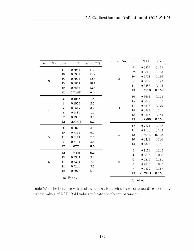
5.5 Calibration and Validation of UCL-SWM
Sensor No. Run NSE α1(×10−3)
3
17 0.7954 11.9
16 0.7934 11.2
18 0.7924 12.6
15 0.7859 10.4
19 0.7848 13.3
12 0.7247 8.3
4
3 0.4052 1.8
4 0.3952 2.5
5 0.2515 3.2
2 0.1883 1.1
52 0.1331 3.6
12 -2.4041 8.3
5
9 0.7341 6.1
10 0.7334 6.9
11 0.7119 7.6
8 0.7100 5.4
12 0.6724 8.3
6
12 0.7441 8.3
13 0.7366 9.0
11 0.7320 7.6
14 0.7121 9.7
10 0.6977 6.9
(a) For α1.
Sensor No. Run NSE α2
3
9 0.6827 0.129
32 0.6819 0.133
10 0.6778 0.136
8 0.6682 0.123
11 0.6587 0.142
13 0.5910 0.154
4
16 0.3653 0.173
15 0.3628 0.167
17 0.3506 0.179
14 0.3391 0.161
18 0.3223 0.185
13 0.2890 0.154
5
12 0.7274 0.148
11 0.7126 0.142
13 0.6974 0.154
10 0.6401 0.136
14 0.6326 0.161
6
5 0.7159 0.105
4 0.6893 0.098
6 0.6249 0.111
3 0.4935 0.092
7 0.4522 0.117
13 -1.2847 0.154
(b) For α2
Table 5.5: The best five values of α1 and α2 for each sensor corresponding to the five
highest values of NSE. Bold values indicate the chosen parameter.
189

5.5 Calibration and Validation of UCL-SWM
0
0.1
0.2
0.3
Sensor No. 3ObservedSimulated
0
0.1
0.2
Hsig(m
)
Sensor No. 4Simulated. incl. island
0
0.1
0.2Sensor No. 5
04 00:00 04 12:00 05 00:00 05 12:00 06 00:00 06 12:00 07 00:00
0
0.05
0.1
0.15
Time
Sensor No. 6
(a)
0
0.5
1
1.5 Sensor No. 3
0
0.5
1
Tp(s)
Sensor No. 4
Simulated. incl. island
0
0.5
1
Sensor No. 5
ObservedSimulated
04 00:00 04 12:00 05 00:00 05 12:00 06 00:00 06 12:00 07 00:00
0
0.5
1
1.5
Time
Sensor No. 6
(b)
Figure 5.25: Comparison of observed versus best simulation series of a) Hsig; and b)
Tp for each sensor location for 3 to 8 of April 2011.
190

5.5 Calibration and Validation of UCL-SWM
0 0.1 0.2 0.30
0.1
0.2
0.3
Sensor No. 3
Sim
ulatedH
sig(m
)
0 0.05 0.1 0.150
0.05
0.1
0.15
Sensor No. 4
0 0.1 0.20
0.05
0.1
0.15
0.2
Sensor No. 5
Sim
ulatedH
sig(m
)
Observed Hsig (m)0 0.05 0.1 0.15
0
0.05
0.1
0.15
Sensor No. 6
Observed Hsig (m)
(a)
0 0.5 1 1.50
0.5
1
1.5
Sensor No. 3
Sim
ulatedTp(s)
0 0.5 10
0.5
1
Sensor No. 4
0 0.5 10
0.5
1
Sensor No. 5
Sim
ulatedTp(s)
Observed Tp (s)0 0.5 1 1.5
0
0.5
1
1.5
Sensor No. 6
Observed Tp (s)
(b)
Figure 5.26: a) Simulated against observed Hsig; and b) Tp for the period 3 to 8 of
April 2011. Simulated series for sensor 4 includes the effects of the lake island.
191

5.5 Calibration and Validation of UCL-SWM
Table 5.6: Summary statistical information for simulated and observed wave parame-
ters between 3 and 8 April 2011. Information for the simulated data at site 4 includes
the effects of the lake island referred to in the text.
Site 3 Site 4 Site 5 Site 6
Obs. Sim. Obs. Sim. Obs. Sim. Obs. Sim.
Maximum (m) 0.32 0.22 0.19 0.19 0.23 0.22 0.19 0.17
Mean (m) 0.15 0.13 0.08 0.12 0.11 0.13 0.09 0.10
Std. Dev. (m) 0.07 0.04 0.04 0.03 0.05 0.03 0.04 0.02
Corr. Coef. 0.86 0.85 0.91 0.89
RMSE (m) 0.05 0.04 0.03 0.02
Linear fit.:
-Slope 0.44 0.55 0.58 0.54
-Intercept (m) 0.06 0.07 0.06 0.05
NSE 0.72 0.37 0.67 0.74
(a) Wave Height, Hsig
Site 3 Site 4 Site 5 Site 6
Obs. Sim. Obs. Sim. Obs. Sim. Obs. Sim.
Maximum (s) 1.62 1.25 1.32 1.16 1.27 1.24 1.75 1.17
Mean(s) 1.19 0.94 1.04 0.92 1.01 0.94 1.33 0.87
Std. Dev. (s) 0.16 0.14 0.10 0.09 0.14 0.13 0.20 0.13
Corr. Coef. 0.76 0.73 0.88 0.78
RMSE (s) 0.28 0.14 0.09 0.47
Linear fit.:
-Slope 0.67 0.65 0.83 0.51
-Intercept (s) 0.14 0.24 0.11 0.20
NSE 0.59 0.54 0.70 -1.28
(b) Wave period, Tp
192

5.5 Calibration and Validation of UCL-SWM
Intermittent spikes appear in both the modelled Hsig (Figure 5.25a) and Tp (Fig-
ure 5.25b) series. These are associated with sudden and significant changes in the fetch
given by deviations of the wind from the predominant direction. Comparing the fetch
computed using UCL-SWM and the wind direction at the four locations (Figure 5.27)
it is evident that the fetch is very sensitive to wind direction changes. This means
that small changes in the wind direction will trigger significant changes in the fetch,
which may greatly affect calculations of Hsig and Tp. The occurrence of these spikes
caused by sudden increase in the fetch will become more frequent for more complex
and irregular basin shapes.
0
500
Sensor No. 3
0
200
Fetch W. Dir.
0
500
Fetch
(m)
Sensor No. 4
0
200
Winddirection
(o)
Fetch incl. island
0
500 Sensor No. 5
0
200
04 00:00 04 12:00 05 00:00 05 12:00 06 00:00 06 12:00 07 00:00
0
500
Time
Sensor No. 6
0
200
Figure 5.27: Comparison between fetch and wind direction at the different sensor
locations for period 3 to 8 of April 2011.
More generally, discrepancies between simulated and observed Hsig and Tp might
originate in various ways. One of the common mistakes in the set-up of wind-wave
193

5.5 Calibration and Validation of UCL-SWM
propagation models is that the time at which the waves are triggered is computed
wrongly, so the arrival time and the frequency of waves are affected (Hawley et al.,
2004). Also, since UCL-SWM is based on linear wave theory, the estimation of the
wave information is made at every point of the computational grid without considering
the effects induced by its neighbours. The bi-directional propagation of waves and pro-
cesses such as diffraction and refraction of waves are not considered. This bi-directional
behaviour is particularly important near the shoreline because when waves break, sec-
ondary currents and oscillations are initiated, which feedback into the incident waves.
Errors in the estimation of Hsig and Tp are also induced by the way that the wind field
is introduced (Schwab et al., 1984, Hawley et al., 2004). Although the wind forcing
in Llyn Conwy was set up to be spatially uniform over the whole lake, a more precise
spatial distribution of the wind field might improve the simulation of wave propagation,
by considering the effects of wind gradients locally on the displacement of waves.
The advantages of modelling wind-wave bi-dimentional propagation is easily visu-
alized by comparing Hsig and Tp maps (Figure 5.28) computed using UCL-SWM and
the spectral wave model, SWAN (Booij et al., 1999), for Ws = 12 m s−1 and Wd = 210o
(the most frequent wind forcing conditions in Llyn Conwy). Whereas UCL-SWM does
not consider a 2D bidimensional propagation, SWAN is a bidimensional model which
includes quadruplet wave-wave interactions, bottom friction, and depth-induced wave
breaking. Such SWAN features significantly influence the discrepancies between both
calculations that occur especially along the sectors of longer fetches, where relative
spatial discontinuities toward the central and eastern sectors coincide with significant
contiguos fetch changes. Despite the spatial differences, the magnitude of Hsig and Tp
are quite similar for both models and discrepancies are below 10%.
Significant differences exist between the computational performance of UCL-SWM
and SWAN. Clocking the run time of both models on a Sun Ultra 24 workstation with
3 GHz Intel quad-core processor, shows that whereas UCL-SWM takes 1 s, SWAN
requires 10 s. The much longer time required by SWAN is because it uses an implicit
numerical scheme where performance is linked to numerical convergence, which is quite
sensitive to bathymetric resolution, boundary conditions and wind forcing data. Com-
putational performance can be more critical when SWAN is coupled with 3D hydrody-
namic models (e.g. Zhang & Li, 1997, Warner et al., 2008), because the data exchange
between models usually increases run time and required expertise to determine the op-
timum synchronization interval. UCL-SWM thus offers a robust and computationally
194

5.5 Calibration and Validation of UCL-SWM
efficient alternative suitable to couple with 2D/3D hydrodynamic models to estimate
the wind-wave parameters in complex lake basins.
North(m)
North(m)
North(m)
North(m)
North(m)
North(m)
North(m)
North(m)
North(m
)
Hsig(m
)
(a) UCL-SWM , Hsig
North(m)
North(m)
North(m)
North(m)
North(m)
North(m)
North(m)
North(m)
North(m
)
Hsig(m
)
(b) SWAN, Hsig
North(m)
North(m)
North(m)
North(m)
North(m)
North(m)
North(m)
North(m)
North(m
)
Tp(s)
(c) UCL-SWM , Tp
North(m)
North(m)
North(m)
North(m)
North(m)
North(m)
North(m)
North(m)
North(m
)
Tp(s)
(d) SWAN, Tp
Figure 5.28: Comparison of Hsig and Tp computed with UCL-SWM and SWAN for
Ws = 12 m s−1 and Wd = 210o.
195

5.6 Bottom Stresses for Wind Forcing and Water Level Scenarios
5.6 Bottom Stresses for Wind Forcing and Water
Level Scenarios
5.6.1 Introduction
Analysis of bottom shear stresses resulting from both currents and wind-waves was
undertaken for hypothetical scenarios based on long time series of observed wind speed
and wind direction for the Llyn Conwy catchment, and the observed variation in water
surface level. The selection of wind speed and wind direction scenarios was based on
a frequency analysis of the records from the CEH data buoy and the catchment AWS
(see Figure 2.13) between November 2006 and December 2008, and a longer series for
nearby Capel Curig from August 1993 and August 2011. Since the difference of altitude
between Llyn Conwy and Capel Curig No.3 station is ≈ 238 m, the data recorded at
the station were corrected empirically following the wind profile power law (Justus &
Mikhail, 1976):
Wsz = Ws0
(z
z0
)α
(5.1)
where Wsz is the resultant wind speed at height z, Ws0 is the known wind speed
at height z0, and α is an empirical exponent. A linear regression analysis between
hourly wind speed recorded at the weather stations and at Llyn Conwy for the period
2006-2008 (see Figure 5.29) was used to obtain the optimum value of α. This yielded
a regression equation of the form WsBuoy = 1.29WsCapelCur.. It should be noted that,
since the values z, z0 and the fitted exponent α are known, the fraction in the Equa-
tion 5.1 reduces to 1.29. No corrections were made to the hourly wind direction series
measured at the weather station, since comparison against the records at Llyn Conwy
coincided with the predominance of southwesterly wind.
The frequency analysis of the fitted wind speed series at Capel Curig No.3 began
with a preliminary analysis of the series at different levels of aggregation (see Fig-
ure 5.30). The hourly series contains peak wind speeds over 40 m s−1 during winter
months. The monthly aggregation also shows that the windiest months are at the
beginning and at the end of every year. On the other hand, the yearly wind speed
aggregation shows more subdued interannual variation between 6 and 8 m s−1, with
no evidence for any progressive trend.
196

5.6 Bottom Stresses for Wind Forcing and Water Level Scenarios
0 5 10 15 20 25 30 350
5
10
15
20
25
30
35
40
45
Capel Curig No.3 Ws (m s−1)
r = 0.65
DataWsBuoy = 1.29WsCapelCur.
CEH
Buoy
St.
Ws(m
s−1)
Figure 5.29: Regression analysis between the hourly wind speed measured at the CEH
data buoy and at Capel Curig No. 3, from November 2006 to December 2008.
An analysis of the seasonal variation in hourly wind speed based on the whole 18
year dataset (Figure 5.31) shows that the wind speed varies sustantially year by year
since standard deviations (σ) of the mean wind speed varies between 3 and 10 m s−1
over the year (see Figure 5.31 (b)). The variability is less in summer (σ ≈ 4 m s−1)
when the averaged wind speeds are relatively low (≈ 6 m s−1) and much higher in
winter (σ ≈ 8 m s−1) when averaged wind speeds are around 10 m s−1.
Aggregating by months (see Figure 5.32) shows that the windiest months are Jan-
uary and February, with a monthly mean wind speed close to 10 m s−1, which varies
between 1 m s−1 and 25 m s−1. In contrast, the lowest monthly mean wind speeds
occur in August and September when the mean wind speed decreases to around 7 m
s−1 (range 2 m s−1 to 16 m s−1).
Further analysis by grouping the hourly wind speed data to hour of the day (from
00 h to the 23 h) (Figure 5.33) shows that the wind speed can vary from 0 to over 30
197

5.6 Bottom Stresses for Wind Forcing and Water Level Scenarios
0
50 93 94 95 96 97 98 99 00 01 02 03 04 05 06 07 08 09 10
Hourly Data (Orig.)
0
20
40
Windsp
eed
(ms−1)
Daily mean
0
10
20
Monthly mean
1993 1995 1998 2001 2004 2006 2009 2012
6
8
10
Yearly mean
Figure 5.30: Daily, monthly and yearly aggregations of the hourly wind speed series
based on Capel Curig No. 3 Station data for August 1993 to August 2011 corrected
for the location of Llyn Conwy.
m s−1 at any hour during the day. However, a weakly periodic mean daily behaviour
of wind speed can be discerned. The mean wind speed remains relatively constant
at about 7.5 m s−1 for the first hours of the day. It gradually increases after 07:00,
reaching a maximum value of 9.8 m s−1 at 15:00. Mean wind speed decreases gradually
reaching the initial value of 7.5 m s−1 around 21:00 remaining at this level until the
end of the day. Diurnal wind speed variation is quite commonly encountered in lake
catchments (e.g. Lake Geneva and Lake Kinneret) and has been used to force daily
average hydrodynamic processes in lakes (e.g Lemmin & D’Adamo, 1997; Pan et al.,
2002). The preceding analysis of the wind speed regime for Llyn Conwy allows the
198

5.6 Bottom Stresses for Wind Forcing and Water Level Scenarios
0
10
20
30
40W
ind
spee
d(m
s−
1)
(a)
Data Mean Maximum Minimum
Jan Mar May Jun Aug Sep Nov
2468
10
σ(m
s−1)
Time (hours)
(b)
Figure 5.31: Seasonal analysis of hourly wind speed data. (a) Hourly, mean, maximum
and minimum wind speed. (b) standard deviation (σ) of the mean wind speed. Capel
Curig No. 3 Station data for August 1993 to August 2011 corrected for Llyn Conwy
location.
Jan Feb Mar Apr May Jun Jul Aug Sep Oct Nov Dec
5
10
15
20
Month
Win
dsp
eed
(ms−
1)
Minimum Maximum Mean ± σ
Figure 5.32: Aggregation by months of the inter-annual wind speed series (See Fig-
ure 5.31 (a)). Records taken at Capel Curig No. 3 Station between August 1993 and
August 2011 fitted to Llyn Conwy location.
199

5.6 Bottom Stresses for Wind Forcing and Water Level Scenarios
quantification of three key aspects of the wind forcing scenarios: the range within
which wind speed fluctuates; the calmest and windiest months during an average year;
and the diurnal wind speed variation.
0 1 2 3 4 5 6 7 8 9 10 11 12 13 14 15 16 17 18 19 20 21 22 23
0
10
20
30
40
Hour
Win
dsp
eed
(ms−
1)
Minimum Maximum Mean ± σ
Figure 5.33: Grouping of the hourly wind speed series by hour of the day. Data for
Capel Curig No. 3 Station between August 1993 and August 2011 corrected for Llyn
Conwy location.
Analysis of the wind-wave parameters obtained from the high resolution water level
measurements versus the meteorological data reveals that wind speeds under 12 m s−1
do not generate significant waves capable of sediment resuspension (see Figure 5.34).
Accordingly, a threshold wind speed of 12 m s−1 was applied in setting up the scenar-
ios. A lower threshold has been reported in other studies of sediment resuspension in
estuaries and lakes. For example, Luettich Jr et al., 1990 used wind speeds within a
range of 5 to 6 m s−1 to study the resuspension of sediments in a large shallow lake.
French et al., 2000 studied muddy sediment dynamics in the Blyth estuary, Suffolk UK,
and established a wind speed threshold of 4.5 m s−1 for sediment resuspension. Other
studies by Bengtsson & Hellstrom, 1992 and Chao et al., 2008 considered a wider wind
speed range of between 1 and 12 m s−1.
Frequency analysis of the wind speed time series shows that wind speed follows an
exponential probability distribution function (Figure 5.35a). The most frequent wind
speeds are around 4 m s−1 and wind speeds > 35 m s−1 are very rare. On the other
hand, the frequency analysis of the wind direction time series (Figure 5.35b) shows
200

5.6 Bottom Stresses for Wind Forcing and Water Level Scenarios
0
0.2
0.4 Sensor No. 3
0
0.1
0.2H
sig
(m)
Sensor No. 4
0
0.2
0.4 Sensor No. 5
0 10 200
0.1
0.2
Ws (m s−1)
Sensor No. 6
Figure 5.34: Wind speed (Ws) versus significant wave height (Hsig) at different sensor
locations for 3 to 8 of April 2011. Dashed line indicates the Ws = 12 m s−1 threshold.
201

5.6 Bottom Stresses for Wind Forcing and Water Level Scenarios
clearly a dominant southwesterly wind direction between 200o and 250o. Although
the probability mass functions in Figures 5.35 show individually the most frequent
wind speed and wind direction events, it is useful to know their joint probability of
occurrence. To do this, a joint probability mass function (JPMF) for wind speed and
wind direction (Figure 5.36) was obtained. The JPMF analysis shows that the most
frequent event is represented by a wind speed of 12 m s−1 and a wind direction of 210o.
It is also evident that 210o is the predominant direction for wind speeds between 6 and
14 m s−1 (see Figure 5.36). Table 5.7 summarises the five most probable wind forcing
events.
5 10 15 20 25 30 350
0.02
0.04
0.06
0.08
0.1
0.12
0.14
0.16
Pro
bab
ility
Wind vel. (m s−1)
(a)
0 50 100 150 200 250 300 3500
0.05
0.1
0.15
0.2
0.25
0.3
Wind dir. (o)
Pro
bab
ility
(b)
Figure 5.35: Probability mass functions for a) wind speed and b) direction, computed
for hourly wind forcing series recorded at Capel Curig No. 3 station between August
1993 and August 2011 and corrected for Llyn Conwy location.
Based on the frequency analysis of wind forcing data two different groups of sce-
narios were established: wind direction scenarios and wind speed scenarios. The wind
direction scenarios consider a constant 12 m s−1 wind speed and different wind direc-
tions binned every 45o from 0o (North) to 315o (Northwest). The wind speed scenarios
consider a constant wind direction of 210 o and different wind speeds binned every 4
m s−1 from 12 to 40 m s−1. A summary of the wind forcing scenarios is shown in
Table 5.8.
202

5.6 Bottom Stresses for Wind Forcing and Water Level Scenarios
0100
200300
1020
30
0
0.02
0.04
Wind dir. (o)Wind vel. (m s−1)
Pro
bability
Figure 5.36: Joint probability mass function of the hourly wind speed and wind direc-
tion for Llyn Conwy.
Table 5.7: The five most frequent wind forcing events at Llyn Conwy. Values taken
from the JPMF shown in Figure 5.36.
Id Wind Dir. Bin (o) Wind Vel. Bin (m s−1) Frequency ×10−2
±15 ±1
1 210 12.0 4.5
2 210 10.0 4.2
3 210 14.0 3.9
4 210 8.0 3.8
5 210 6.0 3.2
203

5.6 Bottom Stresses for Wind Forcing and Water Level Scenarios
Table 5.8: Wind forcing scenarios to investigate the bottom stresses due to the com-
bined action of currents and wind-waves. The letter V and D represent the wind
speed and wind direction scenarios respectively. The letters in bold highlight the most
frequent event.
Wind direction bins (o)
0 45 90 135 180 210 225 270 315
Win
dve
loci
tybin
s(m
s−1)
12 D D D D D V D D D
16 V
20 V
24 V
28 V
32 V
36 V
40 V
Despite the very low probability of occurrence of wind speeds > 32 m s−1 (Fig-
ures 5.35a and 5.36), such extremes are included in the scenarios evaluated. The
reason is twofold. First, due to the non-linear relation between bottom stress and sed-
iment entrainment and transport, infrequent high magnitude stress events can be very
significant contributors to overall sediment redistribution. Second, rare stress peaks
can extend sediment resuspension to parts of a lake that are ordinarily dominated by
deposition. Understanding the location and timing of such events is critically impor-
tant for the understanding of the completeness of lake sediment sequences and their
palaeoenvironmental archives.
Along with the wind forcing scenarios, surface water level variations are also con-
sidered. Observations and measurements of water marks on the sluice at the southern
outlet (see Figure 2.12c) indicate that the average water level may drop about -1 m in
summer, when lower rainfall and higher evaporation are compounded by water abstrac-
tion. In contrast, when rainfall events are persistent, excess lake water is discharged
via the outflow at the south leading to a regulated maximum water surface increment
of about +0.5 m. Based on this, four different water surface level scenarios were es-
tablished: -1, -0.5, 0 (’typical’) and 0.5 m. The wind forcing scenarios sumarised in
Table 5.8 were evaluated for each water surface level scenario.
204

5.6 Bottom Stresses for Wind Forcing and Water Level Scenarios
5.6.2 Wind-wave bottom stress
The computation of the wind-wave shear stress (τw) on the lake bottom was made
using UCL-SWM in isolation from the wind forcing (wind speed and wind direction)
and the water surface level (∆level) scenarios.
Wind direction and water surface level scenarios
The results for the wind direction (Wd) scenarios show that the highest maximum
τw = 1.2 N m−2 occurs when Wd = 90o (easterly wind) and ∆level = 0 m (see
Figure 5.37). High values of maximum τw also occur for the same level when Wd = 0o
and Wd = 270o. The maximum stresses computed for ∆level = −0.5 m are slightly
lower than to those computed for ∆level = 0 m. In contrast, the lowest maximum
τw = 0.7 N m−2 occur when Wd = 45o (Northeasterly wind) and ∆level = 0.5 m.
Integration of the maximum τw in Figure 5.37 for each ∆level shows that the
greatest fraction of maximum τw occurs for ∆level = 0 m, and not for ∆level = −1 m
when water depths are the lowest and shallow sectors become more exposed to wave
action. As is expected, the lower fraction of maximum τw occurs for ∆level = 0.5 m
when a large proportion of the lake bed is protected from the action of waves by the
greatest water depths. Similarly, integrating the maximum τw for each Wd, reveals
that the greatest fraction of maximum τw occurs when Wd = 270o (westerly wind) and
Wd = 0o (northerly wind). This is consistent with the maximum value of fetch and
therefore the development of the largest wind-waves. In contrast, the lowest fraction of
maximum τw occurs for Wd = 135o (southeasterly wind) and Wd = 45o (northeasterly
wind) because the relatively short fetch and the less extensive shallow water zones
along these directions impedes the formation of bigger waves.
In general, the homogeneous behaviour of the maximum τw shown in Figure 5.37,
which varies between 0.8 and 1.2 N m−2, demonstrates the low spatial variability of the
bottom shear stresses due to wind-waves in Llyn Conwy for typical and reduced water
levels. In contrast, a notably reduction of τw, which does not exceed 0.8 N m−2, is
observed when the water level rises (∆level = 0.5). On the other hand, the variation of
the maximum τw in terms of wind direction scenarios demonstrate the complex shape
of Llyn Conwy, where the fetch is sustantially different between wind directions. Also,
the distribution of the shallow areas is not concentric to the deepest areas of the main
lake basin. Rather, these are distributed largely toward the south and in places along
205

5.6 Bottom Stresses for Wind Forcing and Water Level Scenarios
the western and eastern shores. Such diversity of fetch and heterogenous distribution
of shallow sectors affects the growth of wind-waves and therefore the magnitude of τw.
−1−0.5
00.5
0
100
200
3000
0.5
1
∆ level (m)Wind dir. (o)
Max
.stress
(Nm
−2)
Figure 5.37: Maximum wind-wave bottom stresses for wind direction and water surface
level scenarios. Wind speed of 12 m s−1.
The potential bottom area resuspended (BAR) was quantified by comparing the
computed bottom stresses against a critical bottom stress (τcri). The selection of τcri =
0.1 N m−2 was made based on a review of diverse studies of sediment resuspension in
lakes (Sheng & Lick, 1979; Kang et al., 1982; Bengtsson & Hellstrom, 1992; Lou et al.,
2000), which indicate the choosen value as the most appropriate. The results, shown
in Figure 5.38, indicate that the % of BAR is very similar among −0.5 < ∆level <
0.5 m (> 2.8%), but less for ∆level = −1 m (BAR < 2%), because as water level
falls, this removes more of the extensive low gradient shallow marginal areas from the
computation. In terms of the wind direction scenarios, the maximum % of BAR (>
2.8%) occurs for Wd = 0o (northerly wind) and Wd = 225o (southwesterly wind). In
contrast, the minimun % of BAR (< 2.5%) will occur forWd between 45 o (northeasterly
wind) and 180o (southerly wind).
The spatial distribution analysis of τw for different wind directions (e.g. Figure 5.39)
shows that the BAR is, for most of the wind direction scenarios, distributed in a band
206

5.6 Bottom Stresses for Wind Forcing and Water Level Scenarios
1
2
3
4 ∆ level = 0.5 m
1
2
3
4
%of
bott
om
are
a
∆ level = 0 m (”typical”)
1
2
3
4 ∆ level = -0.5 m
0 45 90 135 180 225 270 315
1
2
3
4 ∆ level = -1 m
Wind Direction (o)
Figure 5.38: % of bottom area resuspended (BAR) by wave-induced bottom stress
versus wind direction and for different water surface levels. Wind speed is constant at
12 m s−1.
along the shores, exept for Wd = 0o and Wd = 270o where the BAR covers small
shallow inshore areas. τw usually reaches its maximum values close to the shore where
the maximun fetch is reached. On the other hand, analysing the spatial distribution
of τw under different water surface levels (see Figure 5.40), it is observed that the
proportion of BAR remain nearly constant for −0.5 < ∆level < 0.5 m, and decrease
when ∆level = −1 m since some sectors along the shore become dry areas. Observing
the distribution of τw at different levels for Wd = 0o (Figure 5.40a), the BAR around
207

5.6 Bottom Stresses for Wind Forcing and Water Level Scenarios
the western headland and some sectors along the eastern shore disappears as ∆level
decreases, whereas BAR grows in the south of the lake. On the other hand, analysing
the distribution of τw at different levels for Wd = 225o (see Figure 5.40b) it is observed
that the proportion of BAR in the north-eastern bay stays approximately constant
between for −0.5 < ∆level < 0.5 m, and this almost disappears for ∆level = −1
m. At the northern sectors, larger bottom areas might experience resuspension for
∆level ≥ 0 m.
Figure 5.39: Wind-wave shear stresses for different wind directions at ∆level = 0 m
using a constant wind speed of 12 m s−1. The arrows in the wind rose indicate wind
direction. Grey shaded areas correspond to bottom stresses < τcri.
208

5.6
Botto
mStre
sses
for
Win
dForc
ing
and
Wate
rLevelScenario
s
East (m) x 105North (m) x 105
∆level
(m)
(a) Wind direction 0o (Northerly wind).
East (m) x 105North (m) x 105
∆level
(m)
(b) Wind direction 225o (Southwesterly wind).
Figure 5.40: Wind-wave bottom stresses for wind direction and water surface level scenarios. Constant wind speed of 12
m s−1. Grey shaded areas correspond to bottom stresses < τcri.
209

5.6
Botto
mStre
sses
for
Win
dForc
ing
and
Wate
rLevelScenario
s
Win
dsp
eed
and
wate
rsu
rface
levelsc
enario
s
The
computation
ofτw
forw
ind
speed
and
water
surface
levelscen
ariossh
ows
an
approx
imate
linear
growth
ofth
em
axim
umτw
foreach
∆lev
el(see
Figu
re5.41).
The
linear
growth
ofth
em
axim
umτw
ism
oreaccen
tuated
for∆lev
el=
0m
,w
here
the
high
estvalu
eof
the
max
imunτw
isreach
edfor
Ws
=40
ms−
1.In
contrast,
aless
accentu
atedgrow
thin
max
imumτw
isob
servedfor
∆lev
el=
0.5m
,w
hich
reflects
the
factth
atless
ofth
ebed
isex
posed
tow
ind-w
avesw
hen
the
water
surface
rises.
Integratin
gth
em
axim
umτw
inFigu
re5.41
foreach
∆lev
elsh
ows
that
the
greatest
prop
ortionof
max
imumτw
occu
rsfor
∆lev
el=
0m
.Sin
cesim
ilarresu
ltsw
erefou
nd
in
the
analy
sisof
win
ddirection
and
water
levelscen
arios,th
ism
eans
that
∆lev
el=
0m
(i.e.th
eap
prox
imate
’typical’
lakelevel)
migh
tbe
consid
eredto
represen
tth
eop
timum
forth
eoccu
rrence
ofth
em
axim
unτw
and
therefore
forth
em
ostw
idesp
readsed
imen
t
resusp
ension
irrespective
ofth
ew
eather
condition
s.
−1
−0.5
00.5
20
30
40 0
0.5 1
1.5
∆level(m
)W
indsp
eed(m
s−1)
Max. shear stress (N m−2)
Figu
re5.41:
Max
imum
win
d-w
avebottom
stressesfor
win
dvelo
cityan
dw
atersu
rface
levelscen
arios.W
ind
direction
of210
o(sou
thw
esterlyw
ind).
Observ
ing
Figu
re5.42,
itis
clearth
atth
eB
AR
grows
linearly
forW
sbetw
eento
12
and
40ms−
1under
eachw
atersu
rfacelevel
scenario,
excep
tfor
∆lev
el=
−1m
where
the
growth
startfrom
16ms−
1.T
he
linear
beh
aviou
rm
eans
that
the
rateat
which
210

5.6 Bottom Stresses for Wind Forcing and Water Level Scenarios
BAR increases is proportional to the incremental change in Ws. This relationship
might serve to obtain approximate values of BAR by interpolating for Ws within the
range studied.
2
4
6
8
10
12 ∆ level = 0.5 m
2
4
6
8
10
12
%of
bottom
area
∆ level = 0 m (”typical”)
2
4
6
8
10
12 ∆ level = -0.5 m
12 16 20 24 28 32 36 40
2
4
6
8
10
12 ∆ level = -1 m
Wind speed (m s−1)
Figure 5.42: % of bottom area resuspended (BAR) by wind-wave bottom stresses versus
wind speed for different water surface levels. Wind direction of 210 o.
A spatial analysis of the change in BAR with increasing wind speed (see Figure 5.43)
shows that small areas along the north, northeast and east shores of the lake are always
resuspended for any wind speed > 12 m s−1. As wind speed increases, BAR extends
slowly from the northeast toward the southwest, ending as a broader band along the
shore. Towards the southwest of the easterly bay and at the windward side of the
211

5.6 Bottom Stresses for Wind Forcing and Water Level Scenarios
westerly headland, BAR starts to grow at Ws = 24 m s−1. Small central bottom
sectors in the south can be also resuspended when Ws ≥ 36 m s−1.
Figure 5.43: Wind-wave bottom stresses for wind speed scenarios, ∆level = 0 m and
constant wind direction of 210 o (Southwesterly wind). Grey shaded areas correspond
to bottom stresses < τcri.
212

5.6 Bottom Stresses for Wind Forcing and Water Level Scenarios
5.6.3 Current-induced bottom stress
The bottom shear stresses produced by currents (τc) were computed using FVCOM
in steady-state mode, for each of the wind direction and wind velocity scenarios, and
the water surface level scenarios. FVCOM was run at variable time steps to guarantee
numerical stability under higher wind speeds.
Wind direction and water surface level scenarios
The analysis of maximum τc (see Figure 5.44) for different wind direction scenarios at
different water surface levels shows that the highest maximum τc is equal to 0.05 N
m−2 and occurs when Wd = 90o and ∆level = 0.5 m. Integrating the maximum τc for
each wind direction in Figure 5.44 yields that the highest proportion of maximum τc
occurs when Wd = 90o. On the other hand, integrating Figure 5.44 for each water level
shows that the proportion of maximum τc is slightly higher for ∆level = 0.5 m.
−1−0.5
00.5
0
100
200
3000
0.01
0.02
0.03
0.04
∆ level (m)Wind dir. (o)
Max
.st
ress
(Nm
−2)
Figure 5.44: Maximum current-induced bottom stresses for wind direction and water
surface level scenarios. Constant wind speed of 12 m s−1.
Interestingly, the τc computed for the wind direction and water level scenarios does
not exceed the τcri. Thus, no resuspension of bottom sediment by currents is predicted
for any combination of wind direction and water surface level when wind speed is ≤
213

5.6 Bottom Stresses for Wind Forcing and Water Level Scenarios
12 m s−1. That said, the spatial distribution of the τc for the wind direction scenarios
(see Figure 5.45) shows that τc is usually higher at the downwind end of the fetch,
where the return flow over the lake bottom reaches its maximum magnitude. However,
for some wind direction scenarios such as Wd = 0o (see Figure 5.46), some mid-fetch
locations are affected by high τc, because the bottom currents are strongly influenced
by the bathymetry. In the particular case of Wd = 0o, those intermediate sectors are
located at the transition between the deeper central basin and the shallower water of
the southeastern shelf. This bathymetric transition zone dissipates part of the energy
of the bottom currents. On the other hand, variation of the water surface level has
little effect on the spatial distribution of τc, but does affect its magnitude and the
extent of the bottom area affected.
Wind speed and water surface level scenarios
The computations of τc for wind speed scenarios show that the maximum τc increases
linearly for each ∆level as the wind speed increases (see Figure 5.47). For ∆level = 0m
the growth of the maximum τc is much more accentuated. By integrating the maximun
τc along each ∆level in Figure 5.47, it is observed that the greatest proportion of
maximum τc will occur for ∆level = 0 m. This result is similar to that already
obtained in the previous section.
The % BAR normally grows linearly fromWs = 24 m s−1 (BAR < 10%) to Ws = 40
m s−1 (where the BAR is > 60%; see Figure 5.48) for all ∆levels. Although the
tendency is similar for all ∆levels, the magnitude of % of BAR for each wind speed
is different and grows in proportion to the increment in water surface level as more
extensive shallow areas are flooded. In all cases, no resuspension of sediments due to
currents is predicted below Ws = 24 m s−1, except for ∆level = 0 m where a small
portion of the area (2%) is resuspended when Ws = 20 m s−1.
The spatial distribution of BAR (see Figure 5.49) shows that bottom areas on the
north and in the northeast of the lake are always affected by Ws ≥ 20 m s−1. These
areas are characterised by strong surface currents that lead to the formation of strong
near-bed return flows that generate high τc values. On the other hand, as wind speed
grows, the BAR begins to expand from the northern and northeastern sectors toward
the soutwestern part of the lake. The expansion is not restricted to this direction,
since BAR simultaneously increases in shallower places along the western and southern
margins where τc is relatively low. It is clear that a large area immediately southeast
214

5.6 Bottom Stresses for Wind Forcing and Water Level Scenarios
Figure 5.45: Current-induced bottom stresses for different wind directions at ∆level =
0 m using a constant wind speed of 12 m s−1. Arrows in the wind rose indicate wind
direction.
215

5.6 Bottom Stresses for Wind Forcing and Water Level Scenarios
East (m) x 105North (m) x 105
∆le
vel
(m)
Figure 5.46: Flow current bottom stresses for wd = 0o at different water surface level
scenarios. Constant wind speed of 12 m s−1.
216

5.6 Bottom Stresses for Wind Forcing and Water Level Scenarios
−1−0.5
00.5
1520
2530
3540
0
0.2
0.4
0.6
0.8
∆ level (m)Wind speed (m s−1)
Max
.stress
(Nm
−2)
Figure 5.47: Maximum current-induced bottom stresses for wind speed and water
surface level scenarios. Wind direction of 210o.
of the lake centre is always unaffected by flow currents even, when wind speed reaches
40 m s−1.
As mentioned above, the % of BAR grows as the water level rises. Figure 5.50
shows that as the water surface level increases new areas, especially along the shores,
are flooded. These are zones where resuspension of sediment is likely. But the incre-
ments of the water surface level are not the only factor that influence the variation
of the BAR. In particular, the lake hydrodynamics are also affected and thus the
configuration of bottom currents, which changes the magnitude and distribution of
τc. Comparing how BAR changes as water surface level increases for two different
wind speeds (Figures 5.50a and 5.50b) it is evident that BAR grows more rapidly for
Ws = 40 m s−1 than for Ws = 24 m s−1 where also, the growth is always around the
same bottom sectors. For both wind speed scenarios it is also observed that northern
and northeastern parts of the lake always experience current-induced bed stresses that
are high enough to resuspend sediments, irrespective of the water level.
217

5.6 Bottom Stresses for Wind Forcing and Water Level Scenarios
12 16 20 24 28 32 36 400
20
40
60
80 ∆ level = -1 m
Wind speed (m s−1)
0
20
40
60
80
%of
bottom
area
∆ level = -0.5 m
0
20
40
60
80 ∆ level = 0 m
0
20
40
60
80 ∆ level = 0.5 m
Figure 5.48: % of bottom area resuspended (BAR) by current-induced bottom stress
versus wind speed and for different water surface levels. Constant wind direction of
210 o.
218

5.6 Bottom Stresses for Wind Forcing and Water Level Scenarios
Figure 5.49: Current-induced bottom stresses for different wind speeds at ∆level = 0
m using a constant wind direction of 210 o (southwesterly wind). Grey shaded areas
correspond to bottom stresses < τcri.
219

5.6
Botto
mStre
sses
for
Win
dForc
ing
and
Wate
rLevelScenario
s
2.7782.78
2.7822.784
3.458
3.46
3.462
3.464
−1
−0.5
0
0.5
Shear Stress (N m−2)
0.1 0.11 0.12 0.13 0.14 0.15 0.16 0.17 0.18 0.19 0.2
East (m) x 105North (m) x 105
∆level(m
)
(a) Wind speed 24 m s−1.
2.7782.78
2.7822.784
3.458
3.46
3.462
3.464
−1
−0.5
0
0.5
Shear Stress (N m−2)
0.1 0.2 0.3 0.4 0.5 0.6 0.7 0.8
East (m) x 105North (m) x 105
∆level
(m)
(b) Wind speed 40 m s−1.
Figure 5.50: Current-induced bottom stresses for wind speed and water surface level scenarios. Wind direction of 210 o
(southwesterly wind). Grey shaded areas correspond to bottom stresses < τcri.
220

5.6
Botto
mStre
sses
for
Win
dForc
ing
and
Wate
rLevelScenario
s
The
analy
sisofτw
andτcfor
the
win
dsp
eed,w
ind
direction
and
water
levelscen
ar-
iosprov
ide
some
poten
tiallyim
portan
tin
sights
into
how
win
dforcin
gdrives
complex
hydro
dynam
icpro
cessesth
at,in
turn
,con
trolth
edynam
icsof
sedim
ent
accum
ulation
.
The
results
clearlyhave
implication
sfor
the
validity
ofth
esed
imen
tfo
cusin
gth
eory
asa
basis
forpred
icting
the
location
ofth
edeep
estan
dm
ostcom
plete
sedim
ent
se-
quen
ces.In
Lly
nC
onw
y,th
ecom
parison
ofτw
andτc
clearlyin
dicates
the
dom
inan
ce
ofτw
overτc
form
uch
ofth
elake
area.C
omparin
gth
em
axim
umτw
(Figu
re5.41)
and
the
max
imumτc
(See
Figu
re5.47)
forth
ew
ind
direction
and
water
levelscen
arios,it
isseen
thatτw
ison
average15
times
greaterth
anτc .
This
iscon
sistent
with
compar-
isons
carriedou
tby
Chao
etal.,
2008,w
ho
found
thatτw
isab
out
tentim
esgreater
than
τc
fora
win
dsp
eedof
10ms−
1in
aox
bow
lake.Sim
ilarly,stu
dies
ofsed
imen
t
resusp
ension
mad
eby
Luettich
Jr
etal.,
1990in
ash
allowlake
found
thatτw
ism
ore
than
tentim
esgreater
than
τc .
Ingen
eral,th
erelative
importan
ceof
these
two
bottom
stresscom
pon
ents
will
vary
dep
endin
gof
the
magn
itude
ofth
ew
ind
speed
.Low
win
dsp
eeds
will
likelycau
seslow
growth
ofτc
and
therefore
aratio
ofτw/τ
cgreater
than
15.B
ut
when
the
win
dsp
eed
ishigh
,τc
grows
more
rapid
lyth
anτw
and
the
ratiodecreases
closerto
1.T
his
ratiois
alsoaff
ectedby
how
the
shallow
erareas
aredistrib
uted
around
the
lake.T
hus,
alarge
expan
seof
shallow
water
dow
nw
ind
will
increase
the
prob
ability
ofth
eoccu
rrence
of
high
erτw
oversu
chareas.
The
analy
sesof
max
imumτw
andτc
computed
forw
ind
speed
and
water
surface
levelscen
arios,in
dicate
that
forboth
the
most
exten
siveareas
ofhigh
bottom
stress
occu
rfor
∆lev
el=
0m
.T
his
contrad
ictsth
ein
tuitive
thin
kin
gth
at,as
water
level
decreases
the
bottom
becom
esex
posed
tow
ind-w
avesan
dcu
rrents,
sostron
gerstresses
will
be
exerted
.H
owever,
the
scenario-b
asedan
alysis
dem
onstrates
that
forw
aterlevels
under
∆lev
el=
0m
much
ofth
epoten
tiallyresu
spen
ded
bottom
areasbecom
edry,
and
the
reduction
ofw
aterdep
thdam
pen
sth
ew
ind-w
avean
dcu
rrent-in
duced
stresses.
The
analy
sesofτw
andτc
versus
win
dsp
eedscen
arioslead
toth
eid
entifi
cationof
certainbottom
areasin
the
north
,north
eastan
deast
ofth
elake
(seeFigu
res5.43
and
5.49),w
ithin
which
bottom
sedim
ents
arelikely
tobe
regularly
resusp
ended
under
a
wid
eran
geof
win
dsp
eeds.
The
distrib
ution
sof
those
areasaff
ectedbyτw
arestron
gly
determ
ined
by
the
fetchgrow
than
dare
preferen
tiallylo
cateddow
nw
ind
along
parts
ofth
esh
orew
here
the
win
d-w
aveen
ergyis
greater.In
contrast,
those
bottom
areas
221
5.7 Combined Current and Wave Bottom Stresses for a Winter Month
affected by high values of τc are more complex to predict since they depend on the
three dimensional behaviour of flow.
5.7 Combined Current and Wave Bottom Stresses
for a Winter Month
The analysis of bottom stress distributions arising under a range of hypothetical wind
forcing and water surface level scenarios provides an idea of which areas of the lake
are susceptible to sediment resuspension by waves and currents. All these scenarios
were computed for steady-state forcing conditions, however, it is important to also in-
vestigate the evolution of the bed stress field under unsteady wind forcing conditions.
Accordingly, this section presents an unsteady analysis of the bottom stresses in Llyn
Conwy for the month of December 1997. As shown in Figure 5.51, this month was char-
acterized by a high mean wind speed (13.4 m s−1) and, in fact, the highest wind speed
between August 1993 and August 2011 occurred in this month (see also Figure 5.31).
December 1997 was also characterised by high wind direction variability (Figure 5.51
(a)), such that a wide range of bottom stress distributions can be expected. As before,
computation of wind-wave bottom stresses (τw) and current bottom stresses (τc) was
made using UCL-SWM and FVCOM respectively.
Bottom stress time series computed at different points distributed around the lake
all show a strong correlation with the wind speed (see Figure 5.52). Wind speed is
better correlated with τw (r ≈ 0.75) for the inshore points (Points 1, 2, 4, and 6)
than with τc (r ≈ 0.67), since the former depends almost linearly on the wind forcing
data, which are explicitely given in the equations resolved in UCL-SWM. The latter
are affected by the non-linear behaviour of the lake circulation. Analysing the bottom
stresses in the inshore points 1, 2 and 4, it is found that τc are low relative to τw
since bottom currents are sustantially dampened in shallow places, in contrast with
wind-waves, which increase in energy on approaching the shore. In the inshore point
6 τw is low relative to τc, since the short fetch at this point impedes the formation
of bigger waves. At offshore points (Points 3 and 5) bottom stresses are only due to
currents since τw are rarely induced at these sectors. Data for point 3, in particular,
demonstrate that the deepest sector of the lake is stronger affected by currents for
Ws > 30 m s−1. At all the near shore locations (i.e. wave sensor sites), bottom stresses
are dominated by τw since flow currents are relatively weak.
222

5.7 Combined Current and Wave Bottom Stresses for a Winter Month
0
100
200
300W
inddir.(o)
(a)
Dec−01 Dec−06 Dec−11 Dec−16 Dec−21 Dec−26 Dec−31
0
20
40
Windvel.(m
s−1)
(b)
Figure 5.51: Hourly wind direction (a) and wind speed (c) from 01 to 31 of December
1997.
The weighted-area spatial average of τw and τc (see Figure 5.53) provides a more
general idea of how bottom stresses vary through time in response to sequential forcing
events. The spatial average stress series also exhibit a high correlation (r = 0.88)
between wind speed and τt. The biggest contribution to that correlation is made by
τw, which has a r = 0.96 with wind speed, whereas r = 0.81 for the relationship between
wind speed and τc. It is observed that 2.3% of the time τt exceeds τcri, which means
that sediment resuspension would likely have occurred during these extremely high
wind forcing conditions. During such sediment resuspension events, τc would contribute
18% of the time whereas the combinations of both type of stresses would contribute
82% of the time, showing that sediment resuspension is mainly due to currents. The
contribution of wind-waves to sediment resuspension may thus be restricted to very
shallow areas, in contrast with bottom currents where resuspension would come also
from medium and deeper sectors too.
An indication of the proportion of the lake bed affected by sediment resuspension
during December 1997 is given by Figure 5.54. This analysis shows that, on average
during the whole month, 4.4% of the bottom area is resuspended by τt, 2.8% by τw and
1.6% by τc. It is notable that about 10% of the lake bottom is eroded continuously by
223

5.7 Combined Current and Wave Bottom Stresses for a Winter Month
0
20
40W
s(m
s−1)
0
0.5Point 1 (Wave sensor 5)
Wind-waves (τw)Currents (τc)Total (τt)
0
0.5
1
Point 2 (Wave sensor 3)
0
0.1
Bottom
stress
(Nm
−2)
Point 3 (CEH Data Buoy)
0
0.5
Point 4 (Max. fetch)
0
0.2
Point 5 (Sediment core)
Dec−06 Dec−11 Dec−16 Dec−21 Dec−26 Dec−31
0
0.05
0.1
Point 6 (Wave sensor 6)
Figure 5.52: Wind-wave, current-induced and total bottom stresses between 01 and 31
of December 1997 at different points in Llyn Conwy. See Figure 5.55 for the location
of points. Horizontal broken line represents estimated τcri. Note different scales on
vertical axes.
224

5.7 Combined Current and Wave Bottom Stresses for a Winter Month
0
20
40
Ws
(ms−
1)
Dec−06 Dec−11 Dec−16 Dec−21 Dec−26 Dec−31
0
0.05
0.1
0.15
0.2
Mea
nst
ress
(Nm
−2)
τwτcτtτcri
Figure 5.53: Weighted-area spatial average of wind-wave, current-induced and total
bottom stresses between 01 and 31 of December 1997.
τw between the 5 and 13 of December, whereas the % of bottom area resuspended by
τc in the same period is affected only intermittently for short periods (but with more
intensity). During the maximum wind speed event (around 25 of December) about
83% of the lake bottom is resuspended, where τc contributes with 95% and τw with 5%
of this area.
A spatial analysis of bottom areas resuspended (BAR) (see Figure 5.55) shows that,
of the 4.4% of BAR by τt, nearly 95% is located along the northerly, northeasterly and
easterly shores, and the 5% remaining corresponds to isolated areas on the southern
margin of the lake. This distribution coincides broadly with the steady state south-
westerly wind direction and multiple wind speed scenarios analysed in the previous
section. Here and in the scenario results, the resuspension zones were mainly deter-
mined by the action of wind-waves whose maximum energy was expected along the
northeasterly shore. However, for higher wind speeds (> 20 m s−1) current bottom
stresses contribute significantly to sediment resuspension in most diverse areas. Cur-
rents might also play a role in the transport of resuspended sediments away from these
areas towards the southerly and westerly areas, where deposition might be favoured.
An analysis of the temporal variation of % of BAR at different water depth ranges
(Figure 5.56) shows that only at the shallower depth range at least a sector of the
225

5.7 Combined Current and Wave Bottom Stresses for a Winter Month
Dec−06 Dec−11 Dec−16 Dec−21 Dec−26 Dec−31
0
20
40
60
80
100%
ofresu
s.bottom
area
Wind-waves (τw) Currents (τc) Total (τt)
Figure 5.54: % of bottom area resuspended by wind-wave, current-induced and total
bottom stresses between 01 and 31 of December 1997.
lake is resuspended at every hour during the whole month due mainly to the action
of τw. As the depth increase resuspension events are limited to extreme wind forcing
conditions and only due to the action of τc. Averaging the % of BAR along the time at
different water depth ranges (Figure 5.57), only those % BAR due to τw have a fairly
consistent tendency to decrease with depth, but only from 0 to 6.6 m. The behaviour
of the % of BAR due to τc does not decrease with depth but instead has a gaussian
distribution where the maximun is in the intermediate depth-range of 6.61-8.81 m.
This behaviour mean that the flow circulation is stronger at the depth-range of 6.6-8.8
m, so the transportation of sediments eroded at shallower areas mainly by wind-waves
is likely to be more intensive at these depths. Such a strong circulation is observed
in Figure 5.14 along the depth-range of 6.6-8.8 m, where a vertical circulation in the
upper half of the section yields a maximun velocity at this range. The % of BAR due
to τt decrease consistently from the shallower areas where the contribution is mostly
made by τw to the deepest sectors where the contributions is only made by τc. The
behaviour of % of BAR at deepest areas indicates that despite the depth, sediment
deposits could be eroded by currents.
The Hakanson, 1984 approach to classifying the lake bottom, which divides it into
erosion, transport and accumulation zones based on water depth and fetch, shows that
226

5.7 Combined Current and Wave Bottom Stresses for a Winter Month
East(mx105)
East(mx105)
East(mx105)
East(mx105)
East(mx105)
East(mx105)
East
(mx10
5)
Meantotalstress
(Nm
−2)
Figure 5.55: Average of the total bottom stresses during December 1997. Grey shaded
areas correspond to bottom stresses < τcri. Numbered squares correspond to location
of the time-series plotted in Figure 5.52. The vectors indicate the mean velocity field
at the bottom.
the erosion zone will generally grow as function of fetch and will cover the bottom areas
above 20 m depth. In contrast, the transportation zones will be those areas below the
erosion zone but not deeper than about 40 m depth and the accumulation areas will
correspond to areas below 40 m. This classification serves as a starting point for iden-
tifying the spatial extent of the sediment remobilization. An approximate sub-division
of these zones in Llyn Conwy based on Figure 5.57 indicates that the erosion zones
would be constituted by those shallow areas between 0 and 5 m affected mostly by
wind-waves, transportation sectors would correspond to those located between 5 to 15
227

5.7 Combined Current and Wave Bottom Stresses for a Winter Month
0
50
100 Depth: 0 - 2.2 m
Wind-waves (τw) Currents (τc) Total (τt)
0
50
100 Depth: 2.2 - 4.4 m
0
50
100 Depth: 4.4 - 6.6 m
0
50
100 Depth: 6.6 - 8.8 m
0
50
100
%of
resu
s.bottom
area
Depth: 8.8 - 11 m
0
50
100 Depth: 11 - 13.2 m
0
50
100 Depth: 13.2 - 15.4 m
0
50
100 Depth: 15.4 - 17.6 m
0
50
100 Depth: 17.6 - 19.8 m
06 11 16 21 26 31
0
50
100
Time (days)
Depth: 19.8 - 22 m
Figure 5.56: Temporal variation of resuspended bottom areas (%) at different water
depth ranges due to different bottom stress contributions.
228

5.7 Combined Current and Wave Bottom Stresses for a Winter Month
0 2 4 6 8 10 12
0 − 2.2
2.2 − 4.4
4.4 − 6.6
6.6 − 8.8
8.8 − 11
11 − 13.2
13.2 − 15.4
15.4 − 17.6
17.6 − 19.8
19.8 − 22
Mean resuspended bottom area (%)
Total (τt)Wind-waves (τw)Currents (τc)
Depth (m)
2.2
4.4
6.61
8.81
11.01
13.21
15.41
17.62
19.82
22.02
Depth
(m)
Figure 5.57: Temporal and spatial average of resuspended bottom areas (%) at dif-
ferent water depth ranges due to different bottom stress contributions. Llyn Conwy
bathymetry map shows extent of water depth ranges.
and deposition would occur over the sectors below 15 m depth. However, the nonlin-
earity of the hydrodynamic processes demonstrated in this chapter and the complex
time-variation in meteorological forcing make such prediction more difficult in practice.
Analysing, for example the % of BAR below 15.4 m where, according to hypothetical
zone division deposition of sediments is supposed to occur, intermittent resuspension
due to currents is also predicted. The next chapter investigates the spatial and tempo-
ral variation in the extent of these three sediment transport zones, and the implications
for the applicability of the sediment focusing theory in more detail.
229

Chapter 6
Analysis and Modelling of Lake
Sedimentation
Resume
This chapter examines the dynamics of sedimentation in Llyn Conwy, withreference to sedimentological analysis of its bottom sediments and modelling ofsedimentary processes using FVCOM coupled with the UCL-SWM wind wavemodel. Ekman grab samples of bed material are analysed to determine thespatial extent of sediment accumulation and the physical properties of the de-posits. Suspended sediment settling characteristics are inferred from determi-nations of particle size and density. Results from dated sediment cores provideinsight in historical sediment accumulation rates at two locations within thelake. The dynamics of sediment movement are modelled using hydrodynamicsforced by meteorological data for a one-month period dominated by very strongsouthwesterly winds in an effort to understand the potential for current- andwave-generated bed stresses to influence the spatial extent of erosion and de-position. Modelling results are compared with both the spatial variation in bedcomposition and historical variation in sedimentation, and then used to informan evaluation of the relative importance of sediment focusing processes in LlynConwy.
6.1 Introduction
The resuspension, transport and deposition of sediments in lakes is complex and re-
quires significant physical and human resources to investigate empirically over timescales
230

6.1 Introduction
long enough to capture the full range of environmental conditions. This is especially
true of upland lakes, where sedimentation may be controlled by wind forcing that is
inherently intermittent, and where extreme conditions with long recurrence intervals
may be important in mediating the location, thickness and completeness of bottom sed-
iment sequences. Various early empirical studies attempted to infer the dynamics of
sediment resuspension based on data obtained from arrays of sediment traps combined
with simultaneous wind data (e.g. Kristensen et al., 1992, Bengtsson & Hellstrom,
1992, Luettich Jr et al., 1990). More recently, studies of large lakes have combined
field measurements with computational hydrodynamic models to investigate the sen-
sitivity of sediment dynamics to both current- and wave-generated shear stresses and
the fate of resuspended material (e.g. Blom et al., 1992,Jin & Ji, 2004, Lee et al.,
2005), and the implications of resuspension for sediment and water quality (e.g. Blom
& Toet, 1993, Lee et al., 2007, Jin & Ji, 2004, Chao et al., 2008). To date, however, few
studies have attempted to model spatial variation in sediment accumulation from the
perspective of longer-term lake infilling or have attempted to test the extent to which
infilling can be explained with reference to the various sediment focusing mechanisms.
Accordingly, this chapter considers further the extent to which conventional sediment
focusing processes can account for the occurrence of significant accumulations of lake
sediment and, also, the extent to which sedimentation in the main accumulation zones
of the Llyn Conwy basin can be expected to proceed continuously or else be subjected
to intermittent resuspension.
The Ekman grab samples of bottom sediment obtained in the April 2011 field cam-
paign are first used to map the extent of the sediment accumulation zones. Sediment
samples are analysed for key physical properties, grainsize distribution and particle
settling characteristics. These data are then used to constrain numerical sediment
transport simulations carried out using the suspended sediment module of FVCOM.
FVCOM is run in conjunction with the UCL-SWM wind wave model, driven by me-
teorological data for a one-month period of extreme southwesterly winds, to provide
indicative insights into fine sediment dynamics under conditions of strong wind forcing.
Model runs are used to identify zones of erosion and deposition and the time variation
in sedimentation in relation to variation in wind speed. The preservation potential of
the sediment sequence is also considered in the context at longer term accumulation
rates from 210Pb dated cores and with reference to the likely interval between resus-
pension events. Finally, the modelling results are used to evaluate the extent to which
231

6.2 Analysis of Lake Bottom Sediments
the operation of sediment focusing processes can explain the pattern of sedimentation
in Llyn Conwy.
6.2 Analysis of Lake Bottom Sediments
6.2.1 Spatial extent of lake sediment accumulation
Over the two field campaigns in 2010 and 2011, 28 deployments of an Ekman grab
resulted in sample recovery from 25 locations, with 3 locations returning no sediment.
In addition, five attempts were made to obtain sediment cores, of which four resulted
in the recovery of at least some lake sediment, with one complete core (CONLM1).
The material recovered can be divided into a number of distinct types. Lake muds
comprised either poorly consolidated organic peat or a mixture of peat with clay. In
a few locations, notably in the northeastern part of the basin, a sparse cover of fine
pebbles of compacted peat class (mean diameter ≈ 5 mm) were observed overlying pre-
Holocene deposits of buff clay and silt with a variable fine gravel component. Along
the north shore of the lake and in part of the deepest central basin, no sediment was
recovered, again implying the absence of any Holocene lake sedimentation. Figure 6.1
summarises the distribution of these sediment types. It is notable that much of the
eastern half of the basin is essentially devoid of continuous lake sediment sequences, in
contrast to the western basin and sheltered southern tip of the longer eastern basin.
This is broadly consistent with the wave-stress acting as a mediator of bed sediment
stability. However, it is also clear that deeper parts of the basin that lie well below the
wave base also lack deposits of lake mud.
6.2.2 Physical properties of lake muds
The lake muds (organic peat with small fractions of silt and clay samples) and the silt
and clay fraction of the pre-Holocene samples (i.e. excluding any gravel or fine peat
pebble components) were subjected to further analysis to determine water content, loss
on ignition (LOI) and grainsize distribution. After drying of sub-samples at 105 oC for
6 hours the water fraction (Ww) was computed from
Ww =Wt −Ws
Wt100 (6.1)
232

6.2 Analysis of Lake Bottom Sediments
North(m
)
Figure 6.1: Classification of bottom sediment types based on Ekman grab and coring
attempts during the two field campaigns. Numbers refer to grab samples, CONLM1 is
the core location, and ’x’ denotes coring attempts that yielded sediment information
but no complete core.
233

6.2 Analysis of Lake Bottom Sediments
where Wt is the total weight and Ws is the dry weight of sediments. The spatial
distribution of water content in the bottom sediments (Figure 6.2) reveals two distinct
zones. The first extends over western and southern areas and comprises sediments
with the highest water content (> 75 %). These are generally highly organic and
poorly consolidated peats, including those samples with some clay and silt component.
In contrast, the second zone is distributed across parts of the northwest and eastern
basin, and comprises the pre-Holocene deposits dominated by clays and silts with a
lower water content (< 45 %).
North(m
)
Figure 6.2: Distribution of % of water content in Llyn Conwy bottom sediments.
LOI was used as a proxy for the % of organic matter (Worg). Dried sub-samples
were heated at 550 oC in a furnace for 2 hours and Worg computed from
Worg =Ws −WNorg
Ws
100 (6.2)
where WNorg is the inorganic fraction (e.g. mineral content) in the sample.
234

6.2 Analysis of Lake Bottom Sediments
The spatial distribution of Worg (Figure 6.3) shows an slightly heterogeneous pat-
tern. The highest Worg (> 60%) is found in an small area located at the most southern
part of the lake. Here, one of the few streams within the catchment flows into a
sheltered area of shallow water. A more extensive area is covered by sediments with
25 < Worg < 60%. In contrast, the lowest Worg values (< 20%) are observed in the
east, northeast and centre of the lake where lake muds are absent and pre-Holocene
clays persist on the bed.
North(m
)
Figure 6.3: Distribution of % of organic matter (Worg) in Llyn Conwy bottom sedi-
ments.
There is a strong correspondence between the spatial distributions of Worg and
Ww distributions. This is unsurprising since sediments with high organic content are
generally characterised by high porosity (see, for example, Hakanson & Jansson, 1983).
A linear correlation analysis between Worg and Ww yielded R2 = 0.72 (n = 25, p =
0.02).
235

6.2 Analysis of Lake Bottom Sediments
6.2.3 Sediment size distributions
All samples were additionally subjected to grain size analysis using a Malvern Master-
Sizer 2000 laser granulometer. Grainsize was computed and selected summary statistics
(median (d50) diameter, sorting and sediment classification) determined using the Folk
& Ward, 1957 arithmetical measures. Two sets of analyses were run. The first was
conducted using gently agitated samples; the second included 10 minutes of ultrasonic
pre-treatment to disaggregate any composite particles. The resulting grainsize distri-
butions are summarised in Figures 6.4, 6.5 and 6.6. Each distribution represents the
average of three successive laser granulometer analyses. Distributions are grouped into
the three main bottom sediment types: organic peat; clay-rich peat; and pre-Holocene
clay. Curves for samples with and without ultrasonic pre-treatment are shown. Ultra-
sonic pre-treatment invariably results in a significant shift in the both the mode and
median particle size, although these shifts are smaller for some of the pre-Holocene
samples. With the exception of sample 27, areas lacking in Holocene lake sediments
are characterised by much finer clay-rich silts (d50 approximately 11 to 13 µ). Summary
statistics for samples, grouped by sediment type, are provided in Table 6.2. Based on
conventional classificatory schemes (e.g. Blott & Pye, 2001), the ultrasonically-treated
lake muds all lie in the coarse silt range, and most are poorly sorted, with some very
poorly sorted (see Figures 6.7, 6.8 and 6.9).
6.2.4 Density and settling velocity
The bulk density (ρbs) for each sediment sample was estimated using the density bottle
technique, which offers good accuracy for the analysis of soft lake bed sediments (Hilton
et al., 1986b). As seen in Table 6.2, the sediment density is very low owing to the high
organic fraction. Computed densities were then used in conjunction with the Stokes
settling law to to estimate the settling velocity (ws). This assumes spherical particles
settling in a quiescent and homogeneous water column. The latter is a reasonable
representation of the lake environment. The assumption of spherical particles is clearly
hard to justify, however, given the fibrous nature of the organic component of the lake
deposits. Various modifications to take account of shape effects on settling have been
proposed (e.g. Baba & Komar, 1981; Hallermeier, 1981) but in the absence of any shape
information, the original Stokes formulation has been used here. It is not entirely clear
to what extent the larger reduction in particle size for the peat-dominated samples
236

6.2 Analysis of Lake Bottom Sediments
10−1
100
101
102
103
0
0.5
1
1.5
2
2.5
3
Particle size(µ m)
Volume(%
)
RawUltrasoundMedian
(a) Sample No. 2
10−1
100
101
102
103
0
0.5
1
1.5
2
2.5
3
3.5
4
Particle size(µ m)
Volume(%
)
RawUltrasoundMedian
(b) Sample No. 3
10−1
100
101
102
103
0
0.5
1
1.5
2
2.5
3
3.5
4
Particle size(µ m)
Volume(%
)
RawUltrasoundMedian
(c) Sample No. 4
10−1
100
101
102
103
0
0.5
1
1.5
2
2.5
3
3.5
Particle size(µ m)
Volume(%
)
RawUltrasoundMedian
(d) Sample No. 5
10−1
100
101
102
103
0
0.5
1
1.5
2
2.5
3
3.5
4
Particle size(µ m)
Volume(%
)
RawUltrasoundMedian
(e) Sample No. 8
10−1
100
101
102
103
0
0.5
1
1.5
2
2.5
3
3.5
4
Particle size(µ m)
Volume(%
)
RawUltrasoundMedian
(f) Sample No. 24
Figure 6.4: GSD for organic peat.
237

6.2 Analysis of Lake Bottom Sediments
10−1
100
101
102
103
0
1
2
3
4
5
6
Particle size(µ m)
Volume(%
)
RawUltrasoundMedian
(a) Sample No. 6
10−1
100
101
102
103
0
1
2
3
4
Particle size(µ m)
Volume(%
)
RawUltrasoundMedian
(b) Sample No. 7
10−1
100
101
102
103
0
1
2
3
4
Particle size(µ m)
Volume(%
)
RawUltrasoundMedian
(c) Sample No. 10
10−1
100
101
102
103
0
1
2
3
4
Particle size(µ m)
Volume(%
)
RawUltrasoundMedian
(d) Sample No. 12
10−1
100
101
102
103
0
1
2
3
4
5
Particle size(µ m)
Volume(%
)
RawUltrasoundMedian
(e) Sample No. 18
10−1
100
101
102
103
0
1
2
3
4
5
Particle size(µ m)
Volume(%
)
RawUltrasoundMedian
(f) Sample No. 19
10−1
100
101
102
103
0
0.5
1
1.5
2
2.5
3
3.5
4
Particle size(µ m)
Volume(%
)
RawUltrasoundMedian
(g) Sample No. 23
10−1
100
101
102
103
0
1
2
3
4
5
Particle size(µ m)
Volume(%
)
RawUltrasoundMedian
(h) Sample No. 25
Figure 6.5: GSD for clay-rich peat.
238

6.2 Analysis of Lake Bottom Sediments
10−1
100
101
102
103
0
0.5
1
1.5
2
2.5
3
3.5
4
Particle size(µ m)
Volume(%
)
RawUltrasoundMedian
(i) Sample No. 28
Figure 6.5: Continued.
10−1
100
101
102
103
0
1
2
3
4
5
6
Particle size(µ m)
Volume(%
)
RawUltrasoundMedian
(a) Sample No. 1
10−1
100
101
102
103
0
0.5
1
1.5
2
2.5
3
3.5
Particle size(µ m)
Volume(%
)
RawUltrasoundMedian
(b) Sample No. 9
10−1
100
101
102
103
0
0.5
1
1.5
2
2.5
3
Particle size(µ m)
Volume(%
)
RawUltrasoundMedian
(c) Sample No. 21
10−1
100
101
102
103
0
0.5
1
1.5
2
2.5
3
3.5
Particle size(µ m)
Volume(%
)
RawUltrasoundMedian
(d) Sample No. 27
Figure 6.6: GSD for pre-Holocene clay.
239

6.2 Analysis of Lake Bottom Sediments
Table 6.1: Mean, sorting and sediment classification for each sediment sample based
on the GSDs.
Sample Test Median (µ m) Sorting (µ m) Description
2Raw 59.98 5.03 Very poorly sorted very coarse silt.
Ultrasound 20.79 5.54 Very poorly sorted coarse silt.
3Raw 82.02 3.32 Poorly sorted very fine sand.
Ultrasound 20.97 3.29 Poorly sorted coarse silt.
4Raw 101.54 3.44 Poorly sorted very fine sand.
Ultrasound 21.39 3.50 Poorly sorted coarse silt.
5Raw 68.04 3.55 Poorly sorted very fine sand.
Ultrasound 25.27 4.04 Very poorly sorted coarse silt.
8Raw 125.02 3.57 Poorly sorted fine sand.
Ultrasound 20.38 3.25 Poorly sorted coarse silt.
24Raw 123.70 3.28 Poorly sorted very fine sand.
Ultrasound 23.12 3.39 Poorly sorted coarse silt.
AverageRaw 91.28 3.74 Poorly sorted very fine sand.
Ultrasound 21.930 3.83 Poorly sorted coarse silt.
(a) Organic peat.
Sample Test Median (µ m) Sorting (µ m) Description
6Raw 260.84 4.28 Very poorly sorted medium sand.
Ultrasound 27.33 3.85 Poorly sorted coarse silt.
7Raw 118.39 3.24 Poorly sorted very fine sand.
Ultrasound 21.63 3.38 Poorly sorted coarse silt.
10Raw 115.92 3.59 Poorly sorted very fine sand.
Ultrasound 24.19 3.39 Poorly sorted coarse silt.
12Raw 139.16 3.02 Poorly sorted fine sand.
Ultrasound 29.09 3.65 Poorly sorted coarse silt.
18Raw 332.40 3.60 Poorly sorted medium sand.
Ultrasound 192.49 5.37 Very poorly sorted fine sand.
19Raw 136.55 3.16 Poorly sorted fine sand.
Ultrasound 19.89 3.32 Poorly sorted coarse silt.
23Raw 135.34 3.54 Poorly sorted fine sand.
Ultrasound 23.09 3.47 Poorly sorted coarse silt.
25Raw 146.23 2.80 Poorly sorted fine sand.
Ultrasound 29.69 3.34 Poorly sorted coarse silt.
28Raw 122.86 3.39 Poorly sorted very fine sand.
Ultrasound 18.46 3.19 Poorly sorted coarse silt.
AverageRaw 152.06 3.58 Poorly sorted fine sand.
Ultrasound 26.02 4.00 Poorly sorted very coarse silt.
(b) Clay-rich peat.240

6.2 Analysis of Lake Bottom Sediments
Table 6.2: Continued.
Sample Test Median (µ m) Sorting (µ m) Description
1Raw 115.70 6.35 Very poorly sorted very fine sand.
Ultrasound 13.12 3.42 Poorly sorted medium silt.
9Raw 24.04 5.88 Very poorly sorted coarse silt.
Ultrasound 11.28 5.12 Very poorly sorted medium silt.
21Raw 14.33 5.01 Very poorly sorted medium silt.
Ultrasound 11.90 5.38 Very poorly sorted medium silt.
27Raw 144.98 5.79 Very poorly sorted fine sand.
Ultrasound 43.82 8.65 Very poorly sorted very coarse silt.
AverageRaw 40.23 6.95 Very poorly sorted very coarse silt.
Ultrasound 14.65 6.25 Very poorly sorted medium silt.
(c) Pre-Holocene clay.
10−1
100
101
102
103
0
0.5
1
1.5
2
2.5
3
3.5
4
Particle size(µ m)
Volume(%
)
← Clay → ← Silt → ← Sand →SampleSample averageMedian
(a) Without ultrasound pre-treatment.
10−1
100
101
102
103
0
0.5
1
1.5
2
2.5
3
3.5
4
Particle size(µ m)
Volume(%
)
← Clay → ← Silt → ← Sand →SampleSample averageMedian
(b) With ultrasound pre-treatment.
Figure 6.7: Averaged GSD distribution of organic peat.
241

6.2 Analysis of Lake Bottom Sediments
10−1
100
101
102
103
0
1
2
3
4
5
6
Particle size(µ m)
Volume(%
)
← Clay → ← Silt → ← Sand →SampleSample averageMedian
(a) Without ultrasound pre-treatment.
10−1
100
101
102
103
0
0.5
1
1.5
2
2.5
3
3.5
4
4.5
Particle size(µ m)
Volume(%
)
← Clay → ← Silt → ← Sand →SampleSample averageMedian
(b) With ultrasound pre-treatment.
Figure 6.8: Averaged GSD distribution of clay-rich peat.
10−1
100
101
102
103
0
1
2
3
4
5
6
Particle size(µ m)
Volume(%
)
← Clay → ← Silt → ← Sand →SampleSample averageMedian
(a) Without ultrasound pre-treatment.
10−1
100
101
102
103
0
0.5
1
1.5
2
2.5
3
3.5
4
4.5
Particle size(µ m)
Volume(%
)
← Clay → ← Silt → ← Sand →SampleSample averageMedian
(b) With ultrasound pre-treatment.
Figure 6.9: Averaged GSD distribution of pre-Holocene clay.
242

6.2 Analysis of Lake Bottom Sediments
follow ultrasound treatment reflects the existence of more complex post-depositional
aggregations of peat fibres, or whether the ultrasonic treatment is actually aiding the
disintegration of individual peat fragments. Therefore, the raw untreated particle sizes
are used in all the settling velocity calculations. An approximate spatial distribution
of ρbs is shown in Figure 6.10. This reveals two distinctive zones. First, a region of
higher density pre-Holocene clays and silts that are also characterised by higher ws (see
Table 6.2). Second, a region of low density organic lake sediments, with low ws (≤ 0.3
cm s−1).
North(m
)
ρbs
(gcm
−3)
Figure 6.10: Spatial distribution of ρbs in Llyn Conwy.
6.2.5 Historical sedimentation rate
Radiometric dating analysis of the upper 0.40 m of the sediment core (CONLM1)
for 210Pb, 137Cs and 241Am was undertaken in the BEIF at UCL by Dr Handong
Yang. The results of this analysis are summarised in Table 6.3. Total 210Pb activity
reaches equilibrium with the supported 210Pb at a depth of around 0.27 m in this core.
Unsupported 210Pb activities, calculated by subtracting supported from total 210Pb
243

6.2 Analysis of Lake Bottom Sediments
Table 6.2: Diameter (d), bulk density (ρbs), settling velocity (ws) and minimum time
to reach the bed (T ) for Llyn Conwy bottom samples.
Sample d (µ m) ρbs (g cm−3) ws (cm s−1) Depth (m) T (s)
2 60.0 1.8 0.1 3.0 2529
3 82.0 1.9 0.2 5.1 2075
4 101.5 1.8 0.3 2.7 795
5 68.0 2.4 0.3 2.6 945
8 125.0 1.7 0.4 16.2 3616
24 123.7 1.6 0.4 21.2 5711
Mean 91.3 1.7 0.3 8.5 2612
(a) Organic peat.
Sample d (µ m) ρbs (g cm−3) ws (cm s−1) Depth (m) T (s)
6 260.8 2.0 2.9 7.0 244
7 118.4 2.0 0.6 3.9 666
10 115.9 2.2 0.7 9.5 1418
12 139.2 1.9 0.8 20.0 2647
18 332.4 1.6 2.7 4.8 176
19 136.5 1.9 0.7 3.6 507
23 135.3 1.7 0.5 20.4 3824
25 146.2 1.9 0.8 18.1 2337
28 122.9 1.6 0.4 17.5 4742
Mean 146.9 1.9 0.9 12.5 2048
(b) Clay-rich peat.
Sample d (µ m) ρbs (g cm−3) ws (cm s−1) Depth (m) T (s)
1 115.7 1.7 0.4 2.9 774
9 24.4 2.1 0.0 9.0 31676
21 14.3 2.6 0.0 5.0 35355
27 145.0 2.2 1.0 14.5 1391
Mean 40.2 2.2 0.5 7.9 17299
(c) Pre-Holocene clay.
244

6.2 Analysis of Lake Bottom Sediments
activity, decline irregularly with depth. This implies that the sediment accumulation
has varied over time. However, as the decline is more-or-less exponential in nature,
these variations in rate appear to have been fairly gentle. The inventory of unsupported210Pb in the core indicates a mean flux to the core location of c. 31 Bq m−2yr−1. This
is lower than the atmospheric 210Pb deposition flux for this region, which suggests that
this location in the lake has experienced at least some degree of sediment focusing (i.e.
preferential deposition).
Notably, the 137Cs activity versus depth profile Table 6.4 shows that the peak
is significant but at the sediment surface, with a tail of declining activity downwards
within the core. There is also a significant 241Am activity peak in the surface sediments;
below the surface, 241Am activity is below the limit of detection. 241Am fallout was
derived from the atmospheric testing of nuclear weapons and fallout peaked around
1963. Unlike 137Cs, it is generally considered to be essentially immobile in vertical
sediment sequences (Appleby et al., 1991), and thus provides an unambiguous marker
1963 in lake sediment cores. The presence of a 137Cs activity peak at the surface,
together with 241Am implies that the very top of the profile is missing. In some cases,
this can happen through the coring and core handling process. However, this core was
acquired and extruded with great care and with a seemingly intact sediment-water
interface. The conclusion, therefore, is either that there has been a virtual cessation of
sedimentation since the mid-1960s or, more likely, that several cm of surface mud have
been lost through post-depositional reworking.
The core chronology Table 6.5 suggests an average post 1836 rate of sedimentation
of 0.0063 g cm−2 yr−1 or 0.22 cm yr−1. In accordance with the account given by Patrick
& Stevenson, 1986, the rate of sedimentation appears to increase significantly after the
1930s and this is likely due to enhanced sediment production within the catchment. A
second core, CON4 (see Figure 2.13 for location), was acquired in 1987 by researchers
from the ECRC and it is interesting to compare the sedimentation histories at the two
sites. The CON4 core was obtained from a site in the western part of the central basin
in 7.4 m of water. The mean sedimentation rate at this site is 0.28 cm yr−1, which is
very close to that seen in CONLM1. As Figure 6.11 shows, however, the age versus
sedimentation rate curves are quite different. CON4 shows a single prolonged phase
of increased sediment between about 1900 and the 1940s, which then declines through
the 1960s, with minor insignificant peaks into the 1980s. The basal rate is averaged
between 1900 and 1827 but, at 0.21 cm yr−1, and is rather higher than the rates
245

6.2 Analysis of Lake Bottom Sediments
Table 6.3: 210Pb concentrations obtained for core CONLM1.
Depth 210Pb Cum. unsupported
Total Supported Unsupported 210Pb
cm Bq Kg−1 ± Bq Kg−1 ± Bq Kg−1 ± Bq m−2 ±
0.5 735.05 26.59 39.79 4.98 695.26 27.05 91.2 5.1
1.5 319.69 24.76 41.18 5.4 278.51 25.34 199.6 9.5
2.5 259.39 22.8 50.92 5.18 208.47 23.38 263.9 11.9
3.5 225.39 20.11 43.63 4.63 181.76 20.64 319.3 13.8
6.5 185.54 23.29 39.71 5.28 145.83 23.88 460.7 21.9
9.5 225.19 20.43 53.52 4.96 171.67 21.02 605.2 31.1
12.5 198.44 20.97 41.21 4.83 157.23 21.52 758.2 37.6
15.5 108.18 17.44 36.34 4.35 71.84 17.97 853.7 42.1
18.5 102.48 17.64 35.04 8.28 67.44 19.49 914.4 45.2
20.5 108.45 17.79 34.79 4.14 73.66 18.27 956.5 47
21.5 73.77 9.87 41.61 2.64 32.16 10.22 972.1 47.4
23.5 50.81 12.21 48.03 3.34 2.78 12.66 979.7 47.8
24.5 72.07 11.87 39.85 2.96 32.22 12.23 983.5 48.1
26.5 73.83 11.86 48.51 2.95 25.32 12.22 1000.6 48.5
27.5 42.58 8.36 42.21 2.17 0.37 8.64 1002.3 48.7
30.5 49.4 8.75 40.12 2.21 9.28 9.02 1005 49.2
35.5 41.86 10.33 35.64 2.76 6.22 10.69 1023.1 50.3
39.5 49.17 8.86 43.11 2.65 6.06 9.25 1031.1 51.8
for the same period in the CONLM1 core. The CONLM1 curve, in contrast, shows
three distinct peaks in sedimentation around 1840, 1900 and 1960. One interpretation
of this is that this site is generally conducive to sedimentation but also subject to
infrequent erosion under extreme wind forcing events. This would have the effect of
removing poorly consolidated material close to the water-sediment interface, thereby
introducing a step-like discontinuity in the age versus sedimentation curve. Clearly, one
of the main questions to be investigated through the subsequent sediment dynamics
modelling is whether intermittent resuspension is plausible at the CONLM1 site in 9
m of water.
246

6.2 Analysis of Lake Bottom Sediments
Table 6.4: 137Cs, 134Cs and 241Am concentrations in CONLM1.
Depth 137Cs 134Cs 241Am
cm Bq Kg−1 ± Bq Kg−1 Bq Kg−1 ±
0.5 676.43 9.62 0 0 9.62 2.18
1.5 184.06 5.88 0 0 0 0
2.5 90.00 4.34 0 0 0 0
3.5 108.24 4.35 0 0 0 0
6.5 105.37 4.98 0 0 0 0
9.5 95.63 4.35 0 0 0 0
12.5 84.11 3.89 0 0 0 0
15.5 67.10 3.62 0 0 0 0
18.5 44.05 3.36 0 0 0 0
20.5 29.17 2.63 0 0 0 0
21.5 23.47 1.48 0 0 0 0
23.5 20.08 1.94 0 0 0 0
24.5 18.89 1.72 0 0 0 0
26.5 14.72 1.63 0 0 0 0
27.5 13.12 1.17 0 0 0 0
30.5 10.58 1.18 0 0 0 0
35.5 4.43 1.36 0 0 0 0
39.5 6.01 1.20 0 0 0 0
247

6.2 Analysis of Lake Bottom Sediments
Table 6.5: 210Pb chronology of core CONLM1.
Depth Dry mass Chronology Sedimentation rate
Date Age
cm g cm−2 AD yr ± g cm−2 yr−1 cm yr−1 ± %
0 0 1963 47
0.5 0.0119 1960 50 2 0.0041 0.171 6.9
1.5 0.0357 1956 54 2 0.009 0.356 11.1
2.5 0.0623 1953 57 2 0.011 0.401 13.1
3.5 0.0907 1951 59 2 0.0117 0.407 13.4
6.5 0.1774 1943 67 2 0.0116 0.390 18.2
9.5 0.2686 1933 77 3 0.0072 0.235 15.7
12.5 0.3617 1918 92 4 0.0048 0.161 19.3
15.5 0.4493 1902 108 6 0.0064 0.221 31.5
18.5 0.5366 1885 125 9 0.0041 0.138 40.0
20.5 0.5963 1864 146 16 0.0019 0.064 55.4
21.5 0.6274 1851 159 24 0.0029 0.094 80.0
23.5 0.6905 1839 171 30 0.0054 0.170 95.6
24.5 0.7224 1836 174 35 0.0018 0.060 107.6
mean 0.0057 0.1721
248

6.3 FVCOM Sediment Transport Model
0 1 2 3 4 51820
1840
1860
1880
1900
1920
1940
1960
1980
2000
Sedimentation rate (mm yr−1)
Date
CON4CONLM1
Figure 6.11: Sedimentation rate comparison between cores CON4 and CONLM1.
6.3 FVCOM Sediment Transport Model
In order to further understand the dynamics of sedimentation within Llyn Conwy the
FVCOM hydrodynamic and sediment transport models were coupled with the UCL-
SWM linear wind-wave model. To facilitate this, UCL-SWM was pre-compiled as a
Fortran library that can then be called directly by FVCOM. This arrangement equips
FVCOM with the ability to compute the bottom stress due to waves (τw) and combine
this with the current-generated bottom stress (τc) prior to execution of the sediment
transport module. The FVCOM sediment transport sub-model requires information
including the initial concentration of suspended sediments, sediment particle properties
used to compute their transport and settling behaviour (e.g. diameter, density, etc.)
as well as a specification of the vertical variation in bed characteristics. Information on
open boundary inflows and outflows is also required. All of this information is specified
through an external file, as summarised previously in Figure 4.2 (see also Chen et al.,
2004a).
The sediment transport model accommodates multiple (non-interacting) sediment
size fractions. Each class is described by a characteristic grain diameter (d50), particle
249

6.3 FVCOM Sediment Transport Model
density (ρs), critical stresses for resuspension (τcri), and deposition (τcd), and erosion
rate constant (δE), a settling velocity (Ws) and a porosity (Po). Not surprisingly given
the diverse environmental contexts for lake sedimentation modelling, a wide range of
values for these parameters can be found in previous studies. Table 6.6 reviews a
selection of relevant modelling studies. For some parameters there is greater consensus
over the most appropriate value. For τcri, a value around 0.1 N m−2 in used in much of
the literature. In contrast, the values and ranges of τcd and δE are more heterogeneous,
suggesting that these parameters may be more lake-dependent.
250

6.3
FV
CO
MSedim
ent
Tra
nsp
ort
Model
Table 6.6: Literature review of key physical parameters used in lake sediment transport modelling studies.
Reference Sediment class d50 τcri τcd δE ws
(mm) (N m−2) (N m−2) (Kg m−2 s−1) (cm s−1)
Sheng & Lick, 1979Clay and sil. - 5×10⁻²- 1.5×10⁻² - 3.6×10⁻⁵ 7×10⁻³ - 1×10⁻¹
Kang et al., 1982Clay and silt 1×10⁻³-1 0.1 - - -
Luettich Jr et al.,
1990
Clay and fine silt 1.6×10⁻² 5×10⁻² - 1.9×10⁻⁸ - 3.7×10⁻⁵ 2.2×10⁻²
Bengtsson & Hell-
strom, 1992
Sediment flocs 2×10⁻³ 0.15 - 5.56×10⁻⁶ 4×10⁻³
Bailey & Hamilton,
1997
Cohesive, 50% or-
ganic matter.
- - - 2.3×10⁻⁷ - 3.5×10⁻⁷ 3×10⁻³
Lou et al., 2000Silt and sand.
Coarse sand along
shores.
3×10⁻² 5×10⁻² - 0.2 - - 5.8×10⁻³
Jin & Ji, 2004Cohesive - 1.2τcd 0.18 6×10⁻⁵ 1×10⁻³
Lee et al., 2005Silt and clay 0.25 0.1 1.5 1.16×10⁻³ < 8×10⁻²
Chao et al., 2008Clay 2.5×10⁻³ - 3.0×10⁻³ 2×10⁻² 1×10⁻² 1×10⁻⁵ - 4×10⁻⁴ 1×10⁻²
251
6.3
FV
CO
MSedim
ent
Tra
nsp
ort
Model
No
data
exist
with
which
toaccu
ratelyquan
tifycon
temporary
sedim
ent
inputs
into
the
Lly
nC
onw
y.A
lthou
ghtw
osm
allstream
sen
terth
enorth
eastan
dsou
theast
cor-
ners
ofth
ebasin
,th
esehave
not
been
observed
togen
eratevisib
leplu
mes
ofsu
spen
ded
material
under
aran
geof
rainfall
condition
s.H
owever,
durin
gth
eperio
dof
loww
ater
levelin
the
sum
mer
of2010,
peat
dep
ositsw
ereex
posed
where
the
south
easternin
flow
enters
the
lake,im
ply
ing
that
poin
tsou
rcesm
aybe
signifi
cant
attim
es.Such
inputs
may
have
been
more
num
erous
durin
gm
uch
ofth
e20th
centu
ryafter
the
constru
c-
tionof
drain
agech
annels
with
inth
epeat
bog,
especially
inth
eeastern
half
ofth
e
catchm
ent
( Patrick
&Steven
son,
1986).M
ostof
these
have
since
been
blo
ckedan
d
totalsed
imen
tin
put
fromth
ecatch
men
taccord
ingly
reduced
.It
islikely
that
much
ofth
econ
temporary
input
derives
fromerosion
ofth
edep
ositsex
posed
around
the
lakean
dbasal
seepage
emergin
gfrom
the
peat
cover.G
iventh
euncertain
natu
reof
these
bou
ndary
condition
s,it
was
thus
decid
edto
only
undertake
indicative
simula-
tions
ofsed
imen
tex
chan
gesbetw
eenth
ebed
and
the
water
colum
nin
order
toid
entify
zones
oferosion
,dep
ositionan
dresu
spen
sionunder
energetic
metereorological
forcing.
Extern
alsed
imen
tin
puts
areth
us
neglected
.
Sim
ulation
sw
ereru
nusin
ga
single
particle
classw
ithsize
and
settling
character-
isticsgiven
byd
50
=91µ
man
dw
s=
0.3mms−
1,corresp
ondin
gto
the
averagevalu
es
determ
ined
empirically
forth
eorgan
iclake
sedim
ents.
Oth
ersed
imen
tm
odel
param
-
etervalu
esare
givenin
Tab
le6.7.
The
fractionof
sedim
ent
mob
ilisedby
bed
load
transp
ortis
generally
not
signifi
cant
inlakes
(Lee
etal.,
2007)an
dth
em
ainin
terest
here
isth
epattern
oforgan
icsed
imen
taccu
mulation
.B
edload
transp
ortw
asth
ere-
foreneglected
and
only
the
transp
ortof
sedim
ents
insu
spen
sioncon
sidered
.T
he
first
model
run
was
initialised
with
acover
ofsed
imen
tw
ithth
esech
aracteristicsin
alayer
ofin
finite
thick
ness,
effectively
givin
gan
unlim
itedsed
imen
tsu
pply.
This
correspon
ds
toa
transp
ort-limited
situation
and
prov
ides
ausefu
lfirst
insigh
tin
toth
eab
ilityof
the
various
lakehydro
dynam
icpro
cessesto
redistrib
ute
material.
Asecon
dset
ofru
ns
were
initialised
with
a5mm
layerof
mob
ilesed
imen
tw
itha
view
toin
vestigating
am
orerealistic
supply
-limited
redistrib
ution
ofsed
imen
t.T
his
run
was
exten
ded
by
usin
gth
een
dcon
dition
toin
itialisea
second
simulation
with
iden
ticalm
eteorological
forcing
tofu
rther
mitigate
the
artificial
natu
reof
the
initial
state.
The
model
was
forcedby
spatially
uniform
hou
rlyin
tervalw
ind
data
forth
em
onth
ofD
ecember
1997(see
Figu
re5.51)
employed
inth
eearlier
analy
sisin
Chap
ter5.
These
data
were
re-sampled
toa
much
shorter
model
time-step
of1s,
which
was
252

6.4 Analysis of Sediment Dynamics
Table 6.7: Parameter values used in FVCOM sediment sub-model. The last column
indicates the source of the information: [1]lLiterature review (see Table 6.6), [2] analysis
of Llyn Conwy samples.
Parameter Units Values Source
d50 mm 0.091 [2]
ρs Kg m−3 1700 [2]
ws mm s−1 0.3 [1], [2]
δE Kg m−2 s−1 4×10⁻⁵ [1]
τcri N m−2 0.1 [1]
τcd N m−2 0.08 [1]
Po % 0.76 [2]
required to avoid numerical instabilities caused by wind speeds exceeding 30 m s−1.
As noted above, inflows and outflows were neglected and the water balance was assumed
to be static over this short period. Model output included hourly values of suspended
sediment concentration (SSC) at every (x, y, z) location within the computational mesh,
and the net erosion or deposition at every (x, y) location at the bed.
6.4 Analysis of Sediment Dynamics
An initial insight into the temporal variation in SSC in response to wind forcing can be
obtained by considering the spatially-averaged concentrations. Figure 6.12a) shows a
strong correspondence between spatially-averaged SSC for the lake as a whole and the
wind forcing (as represented by the wind speed series). So as wind speed increases above
∼ 12 m s−1 bottom sediments are resuspended, while at lower Ws the concentration
declines proportionally. Integrating the spatial-averaged SSC for each vertical layer
over time (Figure 6.12b) shows a characteristic vertical profile that is consistent with
the familiar Rouse, 1937 profile. The assumption of an unlimited thickness of mobile
sediment across the entire lake bed clearly results in concentrations greater than would
be expected to occur in reality, with an average of around 0.5 mg l−1 in the upper half
of the water column to around 2 mg l−1 at the bottom layer. As Figure 6.12c) shows,
peaks in wind speed result in average concentrations exceeding 10 mg l−1, and over 30
mg l−1 in response to extreme wind speeds of 40 m s−1 (the highest wind speed within
253

6.4 Analysis of Sediment Dynamics
the historical record for this site). SSC rapidly declines after such excursions, and is
almost zero for wind speeds below 12 m s−1.%
ofdep
th
(a)
0.2
0.4
0.6
0.8
1
SSC (mg l−1)
5 10 15 20 25 30 35 40 45
0
20
40
Ws(m
s−1)
0 1 2
SSC (mg l−1)
(b)
Dec−06 Dec−16 Dec−26
0
10
20
Time
SSC
(mgl−
1)
(c)
Figure 6.12: Spatially-averaged suspended sediment dynamics for December 1997 forc-
ing period: a) vertical variation in spatially-averaged SSC; b) space- and time-average
vertical SSC profile; and c) time series of spatially and vertically averaged SSC, with
wind speed series also shown.
Figure 6.13 presents a more detailed analysis of SSC variability along a roughly
north-south transect defining the longest axis of the lake basin for a five-hour period
on 24 December. This period contains the strongest wind forcing and, not surprisingly,
the highest SSC in the simulation performed here. High SSC values are restricted to the
near-bed portion of the water column and are generally highest in shallow zones at the
southern end of the transect, where the bottom gradient is lower, and along the north
shore, where the strongest currents and highest wind-wave heights occur. The wind
254

6.4 Analysis of Sediment Dynamics
speed peaks between 15:00 and 16:00 hours, at which time wind speed exceeds 40 m
s−1, generated waves that cause major resuspension of SSC through the water column
(∼ 5 m depth) in the south part of the lake. It is interesting to note that, whereas
sediments in shallow areas are entrained almost instantaneously as soon as wind speed
rises, entrainment in the deepest places is lagged by nearly an hour after the maximum
intensity of the storm. This indicate that the wind forcing energy is rapidly transmitted
to the bottom via wave-generated stresses in shallow water, whereas in the deepest parts
of the basin the transmission of an incremental increase in wind forcing only takes place
after a strong vertical circulation develops to entrain the bottom sediment.
Analysing the time-averaged spatial distribution of SSC at the bottom layer (see
Figure 6.14a) a narrow band of very high SSC along the northern and eastern shores
is evident where the unlimited supply provided by the bed in this idealised simulation
is exploited by high bottom stresses due to waves. This contrasts with the low SSC
elsewhere in the lake and a steep gradient is evident between the zone of entrainment
and a zone more conducive to deposition. As demonstrated in Chapter 5, waves reach
their maximum height along the northern and eastern shores under the predominant
southwesterly winds, and the predicted significant wave heights under the extremely
high winds driving this simulation reach 0.7 m. The return currents that flow upwind
from the north and east reach values of 0.08 m s−1, and are responsible for extending
the zone of sediment entrainment into deeper water and also transporting suspended
sediments away from the resuspension zone and distributing them into lower energy
areas within the basin. This redistribution process can clearly be observed in the
spatial distribution of SSC at the surface layer (Figure 6.14b)). The distribution of
SSC at the surface layers contrasts with the more localised zones of SSC at the bottom
(which is strongly related to the fetch), and reflects the complex current-driven driven
circulation pathways.
The SSC distribution within the bottom layer is thus much more readily predicted
since this is intimately linked to wind wave generation and propagation along the
fetch. In contrast, the SSC distribution at the surface is more difficult to predict since
it depends on the more complex 3D current circulation. An analysis of SSC at the water
surface at successive hourly intervals during the period of strongest wind forcing (24
December) shows quite clearly how SSC reflects the evolution of the current velocity
field (Figure 6.16). Concentrations are much lower than those at the bed, but the
distinct zones of peak SSC occur in the western and southern margins, far removed
255

6.4 Analysis of Sediment Dynamics
−20
−15
−10
−5
0 1 212:00 (Ws = 24.5m s−1)
Depth
(m)
1
2
−20
−15
−10
−5
0 1 213:00 (Ws = 28.4m s−1)
Depth
(m)
0 200 400 600 800−20
−15
−10
−5
0 1 214:00 (Ws = 31.1m s−1)
Distance (m)
Depth
(m)
1 215:00 (Ws = 33.7m s−1)
1 216:00 (Ws = 41m s−1)
0 200 400 600 800
1 217:00 (Ws = 28.4m s−1)
Distance (m)
SSC (m g l−1)
0 20 40
Figure 6.13: Vertical variation in SSC along a roughly north-south transect (see inset
for location) at successive times during the period of strongest wind forcing between
12:00 and 17:00, day 24. Run initialised with unlimited mobile bed sediment.
256

6.4 Analysis of Sediment Dynamics
(a)
0.08 m s−1
SSC (m g l−1)
2 4 6 8 10
(b)
0.15 m s−1
SSC (m g l−1)
0.2 0.4 0.6 0.8 1 1.2
Figure 6.14: Time-averaged spatial SSC and velocity fields at the bottom (a) and (b)
at the surface for December 1997. Run initialised with unlimited mobile bed sediment.
from the northern and eastern zones of entrainment from the bed. Wind-wave action
in these areas is weak and it seems clear that the relative elevation of surface SSC
in these parts is the result of redistribution by return flows and the circulation more
generally.
A comparison between the SSC patterns for the three scenarios of boundary bottom
sediment supply conditions show few differences. The spatial distribution of SSC for
the unlimited bottom sediment supply scenario (Figure 6.14) and for the 5 mm layer of
mobile bed scenario (Figure 6.15) show similar patterns but a slighly higher extension
of SSC at the bottom layer for the first scenario because of the unlimited supply of
sediment. Comparisons against the third scenario, where the final bottom configuration
of the 5 mm layer of mobile bed scenario is used as the initial condition, indicate that
SSC is reduced since no sediment sources remain.
257

6.4 Analysis of Sediment Dynamics
(a)
0.08 m s−1
SSC (m g l−1)
2 4 6 8 10
(b)
0.15 m s−1
SSC (m g l−1)
0.2 0.4 0.6 0.8
Figure 6.15: Time-averaged spatial SSC and velocity fields at the bottom (a) and (b)
at the surface for December 1997. Run initialised with 5 mm mobile bed sediment.
6.4.1 Spatial pattern of erosion and deposition
Time series of spatially-averaged cumulative erosion and deposition are shown in Fig-
ure 6.17. These more-or-less mirror each other, with the mean rate of erosion exceeding
the mean rate of deposition, since the area dominated by erosion is rather smaller than
that dominated by deposition. Marked inflexions in both curves correspond to intervals
of high wind speed. The net balance between erosion and deposition remains effectively
constant, indicating that transfer of sediment from the bed is mainly restricted to the
lower portion of the water column from which settlement occurs fairly rapidly when the
bottom stress diminishes (over both space and time). This can also be visualised in a
comparison of the average erosion and deposition rates over time (see Figure 6.18). At
wind speeds below about 15 m s−1 the erosion rate is almost zero and this is reflected
in a similarly low deposition rate. In contrast, when wind speed rises above 15 m s−1
marked erosional and depositional events are observed. Here again it should be noted
258

6.4 Analysis of Sediment Dynamics
12:00
24.5
13:00
28.4
14:00
31.1
15:00
33.7
16:00
41
SSC (m g l−1)
0 20 40
17:00
28.4
Figure 6.16: Water surface SSC at successive hourly intervals for period of maximum
wind forcing for December 1997. Arrows indicates indicate wind direction, with wind
speed also given (m s−1). Run initialised with unlimited mobile bed sediment.
259

6.4 Analysis of Sediment Dynamics
that the erosion rates tend to exceed the deposition rates because they are averaged
over a smaller area that predominantly sources material, mainly under the action of
the waves.
01 06 11 16 21 26 31
−10000
−5000
0
5000
Time (days)
(gm
−2)
ErosionDepositionNet flux at the bed
0
20
40
Ws(m
s−1)
Figure 6.17: Spatial-average time series of erosion, deposition and net sediment accu-
mulation. Wind speed (Ws) serie on the top.
Figure 6.19 summarises the spatial pattern of net bed evolution and also the sepa-
rated patterns of net deposition and erosion. Absolute change in bed level is artificially
high under this simulation on account of the unlimited sediment input from shallow
marginal areas. Rates of the order of ±2 cm over 1 month for much of the basin are two
orders of magnitude higher than the recent historical rates inferred from the analysis
of the sediment cores. Sediment deposition is more widely favoured over large parts of
260

6.4 Analysis of Sediment Dynamics
06 16 260
100
200
300
400
Time (days)
(gm
−2h−1)
Erosion RateDeposition rate
0
20
40
Ws(m
s−1)
Figure 6.18: Spatially-averaged time series of erosion and deposition rates. Wind speed
(Ws) serie on the top.
the basin, with erosion being more heterogeneous and highly concentrated in smaller
areas. Depositional areas are preferentially located in the south, west and centre of the
lake. Deposition is relatively high along western margins, including those within the
lee of the main headland. Deepwater accumulation is relatively low and more uniform
over a large extension of the central basin. Areas of rapid deposition broadly corre-
spond to areas of elevated SSC in the surface layer (see Figure 6.14). Erosion ’hotspots’
occur along the northern and eastern shores, where wave-generated bottom stresses are
highest. Certain areas in the west and northwest experience erosion due to the return
circulation currents that flow adjacent to the bed and dissipate on the upwind slope
of the basin. Behind the headland that protrudes from the southern shore, erosion
can also occur due to the strong circulation produced in this bay and, to some extent,
wind-waves.
For the 5 mm mobile bed scenario (see Figure 6.20) the model clearly demarcates
better the zones of erosion and deposition. Due to the limited sediment supply, lower
absolute rates are obtained. Comparing against the extended 5 mm mobile bed sce-
nario results (Figure 6.21), an incremental change from above is observed, with more
subtle zones of erosion and deposition. Lower depositional rates for this last scenario
261

6.4 Analysis of Sediment Dynamics
are broadly comparable with observed historical rates due to the limited supply. This
is therefore a more realistic simulation that clearly differentiates depositional and ero-
sional zones, which coincide broadly with the field observations.
Figure 6.19: Spatial distribution of (a) net bed elevation change (mm); (b) area and
magnitude of deposition (mm); and (c) erosion (mm) at end of model run. Run
initialised with unlimited mobile bed sediment.
6.4.2 Sediment focusing analysis
Sediment focusing is a processes in which sediments are redistributed from shallower
to deeper water by the action of multiple hydrodynamic processes (Likens & Davis,
262

6.4 Analysis of Sediment Dynamics
Figure 6.20: Spatial distribution of (a) net bed elevation change (mm); (b) area and
magnitude of deposition (mm); and (c) erosion (mm) at end of model run. Run
initialised with 5 mm mobile bed sediment.
263
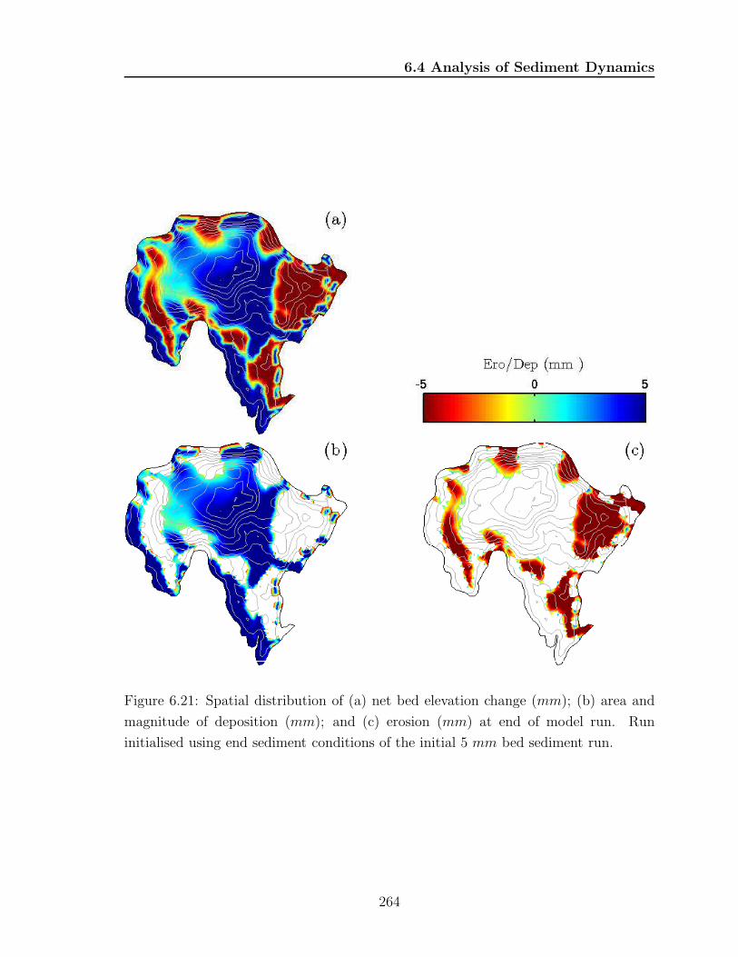
6.4 Analysis of Sediment Dynamics
Figure 6.21: Spatial distribution of (a) net bed elevation change (mm); (b) area and
magnitude of deposition (mm); and (c) erosion (mm) at end of model run. Run
initialised using end sediment conditions of the initial 5 mm bed sediment run.
264

6.4 Analysis of Sediment Dynamics
1975; Blais & Kalff, 1995; Weyhenmeyer et al., 1997). As noted previously, the 210Pb
chronology for the CONLM1 core suggests that a degree of sediment focusing occurs in
Llyn Conwy since the cumulative unsupported 210Pb inventory exceeds the mean atmo-
spheric flux for this region. However, both the distribution of lake sediment deposits
within the basin and the modelled sediment dynamics suggest that the mechanisms
determining sediment accumulation are more complex than envisaged in a simple fo-
cusing model. To further investigate the importance of sediment focusing processes in
Llyn Cowy, the lake bed was divided into 10 different water-depth ranges (Figure 6.22)
and the sediment dynamics in each zone evaluated in detail.
0.5 − 2.72.7 − 4.94.9 − 77 − 9.29.2 − 11.411.4 − 13.613.6 − 15.815.8 − 1818 − 20.120.1 − 22.3
Figure 6.22: 3D perspective view of the spatial distribution of bottom areas for 10
successive water depth (m) intervals.
Curves for cumulative sediment flux at the bed, spatially averaged within each of
these depth zones (see Figure 6.23) reveal several important aspects of the bed dy-
namics. First, it is evident that the shallowest region (0.5≤h<2.7 m) effectively shows
progressive erosion punctuated by stability (with imperceptible deposition) during calm
days. Second, intermediate water depth zones (2.7≤h<13.6 m), exept 4.9≤h<9.2 m
depth zones where an overall erosion is presented, show overall net deposition but this
265

6.4 Analysis of Sediment Dynamics
is punctuated by episodes of erosion under strong wind events. The interplay between
these processes is also evident within times-series of the instantaneous bed flux (see
Figure 6.26). Notably, the depth range from 2.7 to 11.4 m shows a more balanced al-
ternation between deposition and accumulation with little cumulative change relative
to the initial conditions (Figure 6.23). In contrast the zone between 11.4 and 13.6 m
shows a much stronger depositional tendency interrupted only by the most extreme
wind conditions. Third, it is interesting that in the 13.6 to 15.8 m depth zone, the
rate of deposition exceeds that in deeper waters, especially between days 5 and 11 of
the simulation. Finally, in areas deeper than 13.6 m, deposition is clearly the domi-
nant processes (see Figure 6.23). Even here, however, the simulations shows that very
slight erosion can occur on rare occasions when the wind speed exceeds 25 m s−1 (see
Figure 6.26).
Comparing the cumulative sediment flux at the bed within each of the depth zones
given by the unlimited bed supply and the 5 mm mobile bed sediment conditions at
the shallowest region (0.5≤h<2.7 m), the whole 5 mm sediment layer is eroded during
the first strong wind forcing episode around day 6 followed by a strong accumulation
of sediments during the rest of the period (Figure 6.24). This accumulation is pref-
erentially in the western and southern sectors where the wind-wave action is weaker.
More intermediate depths (4.9≤h<9.2 m) are still overall eroded since these are more
affected by currents where erosion and deposition alternate depending on the wind
forcing intensity (see Figure 6.27). Similarly to the first unlimited bed supply scenario,
areas deeper than 13.6 m still show overall net deposition.
The extended 5 mm mobile bed sediment scenario, which is intiated with a conce-
tration provided by the final concentration of the 5 mm mobile bed sediment scenario,
imposes an initial displacement of the curves in Figure 6.25. This scenario shows over-
all net deposition in all the bottom depth zones (Figure 6.25). Erosion of sediments is
limited to episodic wind speeds > 25 m s−1 at those intermediate depths (4.9≤h<13.6
m) affected mostly by currents. Erosion by wind-waves does not occur since sediments
have already been redeposited below the wind-wave base. Deposition is preferently at
the shallower and the deepest areas where the action of currents is weaker see (see
Figure 6.28).
An analysis of the frequency of erosion and deposition in the various depth zones
is presented in Figure 6.29. The frequency of erosion decreases exponentially from
the shallowest waters (h < 2.7 m) where erosion occurs ∼ 64% of the time, to the
266

6.4 Analysis of Sediment Dynamics
01 06 11 16 21 26 31 05
−4000
−3000
−2000
−1000
0
1000
2000
3000
Fluxat
thebed
(gm
−2)
Time (days)
0.5 - 2.7 m
2.7 - 4.9 m
4.9 - 7 m
7 - 9.2 m
11.4 - 13.6 m
13.6 - 15.8 m
15.8 - 18 m
18 - 20.1 m20.1 - 22.3 m
9.2 - 11.4 m
Figure 6.23: Spatially-averaged vertical flux at the bed (deposition positive, erosion
negative) in 10 different water-depth ranges. Run initialised with unlimited mobile bed
sediment.
267

6.4 Analysis of Sediment Dynamics
01 06 11 16 21 26 31 05
−500
0
500
1000
1500
2000
2500
Fluxat
thebed
(gm
−2)
Time (days)
0.5 - 2.7 m
2.7 - 4.9 m
4.9 - 7 m
7 - 9.2 m
9.2 - 11.4 m
11.4 - 13.6 m
13.6 - 15.8 m
15.8 - 18 m
18 - 20.1 m
20.1 - 22.3 m
Figure 6.24: Spatially-averaged vertical flux at the bed (deposition positive, erosion
negative) in 10 different water-depth ranges. Run initialised with 5 mm mobile bed
sediment.
268

6.4 Analysis of Sediment Dynamics
01 06 11 16 21 26 31 05
0
1000
2000
3000
4000
5000
6000
Fluxat
thebed
(gm
−2)
Time (days)
0.5 - 2.7 m
2.7 - 4.9 m
4.9 - 7 m
7 - 9.2 m
9.2 - 11.4 m
11.4 - 13.6 m
13.6 - 15.8 m
15.8 - 18 m
18 - 20.1 m
20.1 - 22.3 m
Figure 6.25: Spatially-averaged vertical flux at the bed (deposition positive, erosion
negative) in 10 different water-depth ranges. Run initialised using end point of initial
5 mm bed sediment run.
269

6.4 Analysis of Sediment Dynamics
−60−40−20
020
0.5 - 2.7 m
Erosion Deposition
050
1002.7 - 4.9 m
−200−100
04.9 - 7 m
−200−100
07 - 9.2 m
−150−100
−500
509.2 - 11.4 m
Bedfluxrate
(gm
−2h−1)
−100
0
100 11.4 - 13.6 m
050
10013.6 - 15.8 m
050
100150 15.8 - 18 m
050
100150
18 - 20.1 m
01 06 11 16 21 26 31
050
100150
20.1 - 22.3 m
Time (days)
Figure 6.26: Time variation in spatially-averaged vertical flux at the bed (deposition
positive, erosion negative) in 10 different water-depth ranges. Run initialised with
unlimited mobile bed sediment.
270

6.4 Analysis of Sediment Dynamics
050
1000.5 - 2.7 m
Erosion Deposition
050
1002.7 - 4.9 m
−150−100
−500
4.9 - 7 m
−100−50
07 - 9.2 m
−100−50
050 9.2 - 11.4 m
Bedfluxrate
(gm
−2h−1)
−150−100
−500
5011.4 - 13.6 m
−200
20406080
13.6 - 15.8 m
050
10015.8 - 18 m
050
100150
18 - 20.1 m
01 06 11 16 21 26 31
050
100150
20.1 - 22.3 m
Time (days)
Figure 6.27: Time variation in spatially-averaged vertical flux at the bed (deposition
positive, erosion negative) in 10 different water-depth ranges. Run initialised with 5
mm mobile bed sediment.
271

6.4 Analysis of Sediment Dynamics
0
50
1000.5 - 2.7 m
Erosion Deposition
0
50
100 2.7 - 4.9 m
−80−60−40−2002040 4.9 - 7 m
−60−40−20
02040 7 - 9.2 m
−500
509.2 - 11.4 m
Bed
fluxrate
(gm
−2h−1)
−500
5011.4 - 13.6 m
−200
204060
13.6 - 15.8 m
050
10015.8 - 18 m
050
100
18 - 20.1 m
01 06 11 16 21 26 31
050
100150
20.1 - 22.3 m
Time (days)
Figure 6.28: Time variation in spatially-averaged vertical flux at the bed (deposition
positive, erosion negative) in 10 different water-depth ranges. Run initialised using end
point of initial 5 mm bed sediment run.
272

6.4 Analysis of Sediment Dynamics
the deepest areas where erosion occurs less than 2.5% of the time. This coincides
with a negative sediment flux at the bed (erosion) in the shallow water zone and
a positive (depositional) flux in deeper water (Figure 6.29 b). The most frequent
deposition (∼ 68%) occurs at intermediate water depths 4.9≤h<7.0 m, and not at the
deepest sectors, where deposition occur less than 40% of the time. This interesting
finding can be explained by the fact that the deepest areas are subject to current
velocities associated with the overall hydrodynamic circulation that lead to long periods
during which the bed stress exceeds the deposition threshold whilst remaining below
the erosion threshold. Such periods of effective bed stability become much less frequent
in shallower water, since they depend on an absence of wave action and therefore calm
weather conditions, which are unusual at this site.
0 50 1000.5 − 2.7
2.7 − 4.9
4.9 − 7
7 − 9.2
9.2 − 11.4
11.4 − 13.6
13.6 − 15.8
15.8 − 18
18 − 20.1
20.1 − 22.3
(a)
Erosion Deposition
Frequency (%)
Depth
(m)
−4 −2 0 2 4
Bed flux rate (g m−2 h−1)
(b)
Figure 6.29: a) Frequency analysis of erosion and deposition within different water-
depth ranges. b) time- and space-averaged bed flux (erosion negative) within different
depth ranges.
These results indicate that sediment focusing in Llyn Conwy occurs partially and in
273

6.4 Analysis of Sediment Dynamics
a complex manner. Sediments are not strictly deposited in the deepest part of the lake,
although its conical shape may favour the deposition in the central basin. Instead, sed-
iments are deposited irregularly in those areas below about 2.7 m reaching a maximum
deposition rate at intermediate depths. The radiometric dating of the CONLM1 core
(obtained in approximately 9 m of water) also suggests that this intermediate depth
zone has been subjected to sediment focusing (see Figure 6.30).
0
20
40(a)
Ws(m
s−1)
−1
0
1
2
(b)
Bed
flux(m
m)
Unlimited supply 5 mm bed layer Extended 5 mm bed layer
01 06 11 16 21 26 31
0
0.2
0.4
0.6
0.8
(c)
Bed
flux(m
m)
Time (days)
Figure 6.30: a) Wind speed; b) bed flux (mm) at the CONLM1 location; and c) at
CON4 location.
A comparison of the sediment bed flux at the two core locations (Figure 6.30) indi-
cates that for the unlimited sediment supply and the 5 mm bed layer supply scenarios
accumulation is the dominant process at both sites. For both scenarios at both sites
there is an overall increase in bed level over the month-long simulation period albeit
274

6.4 Analysis of Sediment Dynamics
with some periods of erosion. The bed flux of sediments is larger at the CONLM1
site since eastern sectors of the lake are subjected to greater current and wind-wave
activity compared to the more calmer zones in the west where CON4 was recovered. At
both core sites, sediment accumulation increases substantially for those periods where
Ws > 10 m s−1, but it is interrupted by erosion events when Ws > 20 m s−1. The
behaviour of the bed flux for the more realistic extended 5 mm bed layer scenario
(see Figure 6.30) supports the suggestion that the top of the CONLM1 core has been
lost. Results for this scenario demonstrate that an overall negative (erosion) bed flux
balance is obtained by the end of the simulation period. In contrast, for the same
scenario sediment accumulation is the dominant process at CON4 site although short-
lived periods of erosion still occur. This supports the hypothesis, based on core dating,
that such western areas are more subject to sediment accumulation. The analysis of
bed flux at both core sites therefore supports the spatial configuration of erosional and
depositional sectors predicted by the model, and also the heterogenity of sedimentary
processes including sediment focusing in Llyn Conwy.
6.4.3 Evaluation of alternative sediment focusing mechanisms
Hilton et al., 1986a identified ten different mechanisms involved in sediment distribu-
tion within small lakes (see discussion in Chapter 1). Only four of those are strictly
implicated in sediment focusing as such, and not all of these are relevant to upland
oligotrophic lakes such as Llyn Conwy. Each is considered further below in the context
of the empirical and modelling evidence presented thus far.
The first factor identified by Hilton et al., 1986a is organic degradation. Llyn Conwy
is very much an oligotrophic system in that it hosts virtually no aquatic macrophytes
and has extremely low turbidity and nutrient loadings. Its catchment is isolated from
urban influences and nutrient-rich discharges. Moreover, the lake is mixed through
most of the year and is only weakly and intermittently stratified during summer. The
low inflow of organic matter and the strong water mixing prevent the onset of anoxia
and eutrophication processes that might otherwise cause the decomposition of organic
matter and sediment focusing in the deepest areas. This mechanism can thus be
completely discounted here.
The second factor involves sliding and slumping within the basin marginal areas.
According to Hakanson, 1977b sediment will not accumulate on slopes > 14%, with
accumulation becoming progressively more likely as the slope declines to 4%. Below
275

6.4 Analysis of Sediment Dynamics
4%, the slope does not impart any significant spatial variation in accumulation. A
map of bottom slope distribution in Llyn Conwy (Figure 6.31a) reveals a concentric
zone of steep slope around the deepest basin in which slopes are relatively high > 10%,
especially along the northern and northeastern shores where slopes attain values up
to 23%. In contrast, more even areas with slopes < 5% are found in the centre of the
basin and within the shallower areas near the western and eastern shores and within
the southern embayment. Slopes around much of the shoreline are relatively consistent
at around 7%, except in the north and northeast shores where the shoreline is steeper,
reaching 13% in places. A summary of spatially-averaged bottom slopes within the
depth zones defined in the preceding section (see Figure 6.31b) reveals that relatively
low gradient areas are preferentially located in the deepest part of the lake, with a
narrower range of shallow depths also characterised by low bed gradients.
The Hakanson classification of bottom slope is applied in Figure 6.31c, from which
it is clear that most of the basin (more than 70% of the bottom area) is likely to
accumulate sediments to at least some degree, whereas the other 30% would favour
mobilisation, either by sliding or by rotational failure, of sediments covering shallower
areas toward the deeper basin. Potential sediment pathways can be visualised by
constructing a slope network of the kind presented in Figure 6.31d. This reveals long
paths that extend from the peripheral areas outside the concentric zone of steepest
slope, especially from the western and northern shores, into the deep central basin.
These could conceivably facilitate sliding of material into the deepest parts of the lake.
A comparison of the slope zones with the observed distribution of bottom sediments
(Figure 6.1) indicates that lake sediments are indeed absent from some areas of steep
slope to the north. The western and southern margins of the deepest basin are, in
contrast, mantled with sediment despite extensive areas of intermediate slope and
localised slopes > 14%. The evidence for slope-control over sedimentation in Llyn
Conwy is thus rather inconclusive. It is certainly a potential factor, and may be
responsible for disturbance to the sediment sequence that the Ekman grab sampling
cannot resolve. Some form of bed imaging (e.g. sidescan sonar) seismic survey would
be required to investigate the prevalence of slope related slides and slumps. An early
application of such techniques by Cronin et al., 1993 to another small upland lake in
Wales did find limited evidence for slumping of highly organic sediments on slopes of
about 15 degrees (26%).
276

6.4 Analysis of Sediment Dynamics
North
(m)
East (m)
North
(m)
North
(m)
East (m)
North
(m)
East (m)
North
(m)
North
(m)
East (m)2.777 2.778 2.779 2.78 2.781 2.782 2.783 2.784
x 105
3.457
3.458
3.459
3.46
3.461
3.462
3.463
3.464
3.465
x 105
0
5
10
15
20
East (m)
North
(m)
Slope(%
)
(a)
0 2 4 6 8 100.5 − 2.7
2.7 − 4.9
4.9 − 7
7 − 9.2
9.2 − 11.4
11.4 − 13.6
13.6 − 15.8
15.8 − 18
18 − 20.1
20.1 − 22.3
Slope (%)
Depth
(m)
(b)
2.777 2.778 2.779 2.78 2.781 2.782 2.783 2.784
x 105
3.457
3.458
3.459
3.46
3.461
3.462
3.463
3.464
3.465
x 105
Slope < 4%4 < Slope < 14%Slope > 14%
East (m)
North
(m)
(c)
2.777 2.778 2.779 2.78 2.781 2.782 2.783 2.784
x 105
3.457
3.458
3.459
3.46
3.461
3.462
3.463
3.464
3.465
x 105
Order
1
2
3
4
5
6
7
8
9
10
11
12
East (m)
North
(m)
(d)
Figure 6.31: Summary analysis of Llyn Conwy bottom slopes. a) Spatial distribu-
tion of bed slope, b) spatial average bottom slope in different water-depth ranges, c)
distribution of bottom areas according Hakanson, 1977b classification, d) downslope
pathways, with colour map indicating network order.
277

6.4 Analysis of Sediment Dynamics
Hilton et al., 1986a also describe a process that they term intermittent complete
mixing, driven by widespread resuspension, mixing, and settling. This leads to sed-
iment focusing by virtue of the greater mass of material in the water column above
deeper areas. The analysis of hourly wind forcing data presented in Chapter 5 re-
vealed high variability in the wind speed record with annually averaged hourly σ ≈ 6
m s−1. The analysis also showed a weak daily periodicity, and wind forcing conditions
dominated by southwesterly winds that can reach 40 m s−1. A persistent overturn
of the thermal structure during winter and autumn, and intermittent and high fre-
quent mixing of water temperature during summer occur as the thermal structure
responds to this meteorological forcing. Such behaviour is only possible in small lakes
such as Llyn Conwy, where the thermocline is rapidly destroyed, thereby allowing the
resuspension of sediment from deeper waters. Wind forcing conditions also lead to
a complex spatial distribution of bottom stress and sediment dynamics around the
lake. Over the duration of the sediment model runs, large incremental increases in
wind forcing drive resuspension of sediments over virtually the entire lake bed via the
action of strong vertical circulation that generates a spatially-averaged τt > 0.5 N
m2. The initial transport-limited model runs predict erosion rates of up to 150 g m−2
h−1 in the shallower northern and eastern areas, accompanied by deposition at a rate
that increases progressively with water depth (see Figure 6.26). Intermittently eroded
marginal sediments are thus efficiently redistributed to intermediate and deeper ar-
eas where the probability of deposition is higher (see Figure 6.29). As established by
Bunge & Bryson, 1956, the occurrence of a stress-drop jet is a major factor in inter-
mittent complete mixing that results in sediment focusing. This phenomenon emerges
in the hydrodynamic simulations of Llyn Conwy and its existence is corroborated by
the flow velocity profiles measured with the ADCP. Both data and model predictions
show that a drastic drop in the wind forcing leads to a reduction of the flow intensity
and also the reversal and attenuation of the vertical circulation in the deepest part of
the basin, leaving the hypolimnion in a quiescent state. The dynamic of both thermal
structure and hydrodynamics are thus consistent with the intermittent complete mix-
ing processes, which can therefore be considered an important mechanism of sediment
focusing in Llyn Conwy.
The fourth mechanism, peripheral wave action is clearly the most important driver
of sediment resuspension in the near-shore regions of Llyn Conwy. This material is
efficiently transported out to deeper water, where settling occurs. Despite the limited
278

6.4 Analysis of Sediment Dynamics
fetch, significant wave heights of 0.3 m commonly occur along the northern and eastern
shores, with heights exceeding 0.5 m under extreme conditions. Combined current and
wind wave modelling shows that the wave-generated bed stresses are typically a order
of magnitude greater than those resulting from currents in shallow water areas.
The frequency of strong winds makes peripheral wave action an important mech-
anism for sediment focusing in Llyn Conwy. Constant exposure to erosion in the
northern and eastern sectors precludes the accumulation of lake sediments, and the
bed is variously made up of coarse lag gravels and relatively resistant pre-Holocene
deposits. Hilton et al., 1986a found that 6% of the total variance of the accumulation
rate estimated by the deployment of sediment traps in Esthwaite water, UK, was due
to wave action. This is manifest as a negative correlation between sedimentation rate
and wind fetch. Deposition rates estimated using sediment traps in lakes located in
the Muskoba-Haliburton region of Canada (Hilton, 1985) similarly indicated that in-
termittent complete mixing and peripheral wave action were the main mechanisms of
sediment focusing.
The above analysis suggests that three of the four mechanisms that Hilton et al.,
1986a associates with sediment focusing can be considered potentially important in Lly
Conwy and possibly within oligotrophic upland lakes in general. Intermittent complete
mixing and peripheral wave action appear to be the most important mechanisms to
explain sediment focusing, since both are consistent with the observed and modelled
hydrodynamics. There is presently no direct evidence to support a role for sliding and
slumping along high gradient downslope pathways.
279

Chapter 7
Discussion
7.1 Introduction
The research presented here has shown that the hydrodynamics and sediment dynamics
of upland lakes are driven by a complex interaction between the incident meteorologi-
cal conditions, the lake bathymetry and the characteristics of the sediments. Processes
such as water thermal stratification, vertical and horizontal circulation and sediment
transport are driven by this interaction and by the interrelationship between these pro-
cesses. Upland lakes are typically characterized by strong but variable meteorological
forcing (e.g. George et al., 2001; Bell et al., 2006). This has been documented here
through analysis of historical records for the Llyn Conwy area. Wind speed at Llyn
Conwy is highly variable (σ ≈ 7 m s−1), especially during winter months when this
varies between 0 and 40 m s−1 . The seasonal temperature is also large with monthly
average air temperature of over 25oC in June and below 4oC in December. Incoming
solar radiation, which is a key variable influencing the lake stratification behaviour,
varies between nearly 100 W m−2 in winter up to 1000 W m−2 in summer.
Bathymetry exerts a major control on both hydrodynamics and sediment dynamics.
In tidal systems, the velocity field may be more sensitive to changes in the bathymetry
than to the bottom roughness (Cea & French, 2012). In lakes with highly complex
bathymetry, the pycnocline turbulence transport varies with bottom slope. About
80% is dissipated where bottom slopes are up to 10%, 60% where bottom slopes are
3%, and less than 7% where bottom slopes are about 0.1% (MacIntyre et al., 2009).
The highly irregular bathymetry of Llyn Conwy is comprised of an extended shallow
(h ≈ 3 m) region in the south and the west where bottom slopes are < 5%, and a deeper
280

7.2 Modelling of Upland Lake Thermal Structure
sector (h ≈ 20 m) towards the centre, where slopes can be up to 22%. The slightly
convex hypsographic area-depth curve indicates a potentially significant exposure of
the lake bottom to wind-wave sediment resuspension.
The study of hydrodynamics and sediment dynamics in upland lakes has been
approached in this thesis by the implementation of computational models. The main
model used is a 3D ocean community code, FVCOM, which has been improved and
adapted for lake problems by the creation of a graphical user interface, FVCOM-GUI
and by the addition of a new wind wave model (UCL-SWM ). A new 1D dynamic model
(UCLAKE ), has also been programmed as a pre-cursor to studies using the 3D model,
to investigate the thermal structure at multiple timescales.
The numerical modelling approach provides new insights into the hydrodynamics
and sediment dynamics, and their relationships, in upland lakes. Such understanding is
crucial in order to provide a scientifically informed context for the coring and analysis
of lake sediments for environmental reconstruction (Hakanson, 1984; Rowan et al.,
1995). The following sections disccuss the key results emerging from the modelling
of hydrodynamics and sediment dynamics in Llyn Conwy and their implications for
the applicability of the sediment focusing theory. Finally, some guidelines for the
optimal acquision of sediment cores are provided in order to improve the robustness of
palaeolimnological studies based on upland lakes.
7.2 Modelling of Upland Lake Thermal Structure
A first step towards the understanding of lake hydrodynamics is the investigation of
the thermal structure, particularly the behaviour of the mixed layer (Imberger, 1985;
Spigel et al., 1986). Knowledge of the time-variation in stratification allows inferences
regarding lake sensitivity to meteorological conditions and, in particular, the intensity
of turbulent mixing through the water column and how frequently the mixed layer is
depened.
A new 1D dynamic eddy-difusivity lake model (e.g. Riley & Stefan, 1988; Hondzo
& Stefan, 1993), UCLAKE, has been implemented and calibrated for Llyn Conwy in
order to investigate the thermal structure over inter-seasonal periods, at daily and
subdaily time scales. A key feature of the model is its ability to dynamically adapt
the numerical timestep to guarantee the good computational performance required for
long-term studies of thermal structure (e.g. Hondzo & Stefan, 1991). The model is
281

7.2 Modelling of Upland Lake Thermal Structure
used to analyse the sensitivity of thermal structure to the important parameters in the
advection-diffusion model of water temperature incorporated into the higher dimension
FVCOM model.
The calibration of UCLAKE was achieved with respect to three parameters: Kzmax,
C and η; commonly subjected to calibration in other eddy difusivity models such as
MINLAKE (Riley & Stefan, 1988). In some similar models (e.g. Hondzo & Stefan,
1993) the calibration procedure is simpler because the highly sensitive Kzmax is esti-
mated as a function of the lake surface area and the buoyancy frequency (N). Other
models (e.g. Henderson-Sellers, 1984) have estimated η as an exponential function of
the secchi-disk depth, but the accuracy of such a function is highly dependent on the
availability of observed data needed to estimate it.
Whilst most 1D lake dynamic models are calibrated and validated against depth-
averaged water temperature time series (e.g. Hondzo & Stefan, 1993; Gal et al., 2003),
calibration of UCLAKE was based on the most appropriate specific temperature in-
formation dimensions (time series or water depth profiles). Following the common
practice, calibration by comparing water temperature time series was initially chosen.
The calibration and sensitivity analysis was carried out at three different depth levels:
surface, middle and bottom, for which different sets of parameter values were obtained.
The results indicate that Kzmax and C decrease in the upper half layer, whereas η in-
creases. The sensitivity analysis shows that, at the water surface layer between March
and April, the model is quite sensitive to changes in any of the three parameters. This
is because, during these months, the lake undergoes a transition from a long period of
overturn to a period of stratification facilitated by a decline in wind speed and the rapid
increase in solar radiation. In the middle layer, from April to December, the model is
very sensitive to changes of Kzmax and η, whereas for C the model is sensitive only
during March and April. In general, the sensitivity of Kzmax and η seems to increase
with depth, especially for summer and autum months, whereas C is only significantly
sensitive between March and April.
An alternative calibration procedure (not reported in detail here) using hourly
temperature profiles yielded different and heterogenous sets of parameters at each time.
Despite this, parameters show certain homegenity by grouping them by months or
seasons. Since this approach was not considered practical because of the difficulties
in grouping parameters (which also affects the parsimony of the model), a calibration
procedure based on water temperature time series was adopted in order to obtain an
282

7.2 Modelling of Upland Lake Thermal Structure
unique value for each unconstrained parameter. The model calibration results indicate
a generally excellent performance with NSE = 0.97 and RMSE = 0.71 oC for Kzmax =
8.90×10⁻⁵, C = 0.2 and η = 2.0 out of 80 model simulations. Similar procedures
applied by Hondzo & Stefan, 1993 to calibrate a 1D dynamic lake model to a wide
range of small lakes, yielded an RMSE of 1.1 oC. In another example, trial and error
calibration of a 1D dynamic lake model of a reservoir by Bonnet et al., 2000, where
the parameters were divided into three different groups: heat exchange, dispersion
processes and inflow and outflows discharges, yielded an RMSE of 0.57 oC.
The performance of UCLAKE is also very good for the validation period, which
lends confidence to the calibrated parameter set values. The model performance yielded
NSE > 0.95 for surface, mid-depth and bottom layer water temperature time series.
The comparisons between observed and simulated water temperature profiles in the
validation period yield an average RMAE of 8.1%, and RMAEs < 10% for 77% of the
validation period. A high RMAE of 50% was found for some short periods in February
and March when the lake is well-mixed and the water temperature falls to ≈ 4oC. To
deal with low water temperature, some models (e.g. Hondzo & Stefan, 1991) include a
threshold under which the model is not able to make any temperature estimation. In
other energy-budget models (Imberger & Patterson, 1981; Spigel et al., 1986) the time-
step is adaptated within a range from 0 to 24 h as a function of subdaily water-surface
energy balance, and the temperature of inflow and outflow. Other sources of discrepan-
cies between observed and simulated temperatures especially at the epilimnetic layers
are probably due to the sensitivity of changes in meteorological information such as
air and dew point temperature (Hondzo & Stefan, 1992). Unreliable wind forcing in-
formation is another source of temperature errors, because most of the components of
the heat energy balance at the water surface depend of this variable (Gal et al., 2003).
The analysis of the thermal structure indicates that the mixed layer only persists for
short continuous periods (< 20 days) in May, June and July. The mixed layer is quite
unstable because of persistent disrruptions of the thermal stratification by the action
of high sustained wind speeds during short periods facilitated by a weak thermocline
(maximun ∆T 6 oC); this allows the continuos stirring of the water column. These
periods are also characterized by having a typical thickness (he) between 2 and 2.5 m,
which can increase up to ∼15 m when sudden increments of wind speed occur. On the
other hand, in autumn, the lake is weakly and intermittent stratified about 30% of the
time because of the low shortwave solar radiation and energetic wind forcing conditions
283

7.3 3D Hydrodynamic Modelling
(averaged Ws = 14.7 m s−1). At the end of spring, the lake is predominantly stratified
(> 70% of the time), facilitated by the relatively low wind speed (< 9 m s−1) and the
rapid increase in shortwave solar radiation. In contrast, during winter the lake is well
mixed nearly 100% of the time because of the low incoming solar radiation and the
high wind speeds.
UCLAKE constitutes a robust and computationally efficient tool for prediction
of lake thermal structure and the behaviour of the mixed layer at sub-daily and daily
scales. The active variations of the mixed layer thickness indicate a rapid lake response
to changes of the meteorological conditions and this implies that such changes may be
potentially important for the resuspension of bottom sediments. Such a response is not
only translated into a mixing mechanism that erodes the thermocline, but also into the
production of complex patterns of internal waves that are not considered explicitly in
1D modelling. The implementation of UCLAKE in Llyn Conwy has served not only
to understand its thermal structure, but also provides insights into the hydrodynamics
and sediment dynamics. The 1D model approach thus serves as a preparatory stage to a
more extensive three-dimensional study of the hydrodynamics and sediment transport
in upland lakes.
7.3 3D Hydrodynamic Modelling
3D hydrodynamic models developed primarily for ocean study cases has been widely
implemented in large lakes (e.g. Jin et al., 2000; Chen et al., 2004b), but their use
in small lakes has been very limited. The use of the 3D hydrodynamic and sediment
dynamic model FVCOM in the upland Llyn Conwy has introduced some new chal-
lenges, such as the design of a computational mesh based on an adequate resolution
and configuration, and an appropriate definition of the bathymetry that minimises
the model uncertainty and improves its performance (e.g Legrand et al., 2006). A
key issue is the mitigation of numerical instabilities caused by the interaction between
high wind speeds and the water body at this exposed upland location. FVCOM has
also been improved by the designing and programming of a graphical user interface,
FVCOM-GUI, to pre- and post-process model information. This makes it much more
comparable with leasing commercial hydrodynamic models such as Delf 3D and MIKE
3D. In addition, a semi-empirical linear wave model, UCL-SWM, has been successfully
284

7.3 3D Hydrodynamic Modelling
incorporated into FVCOM. This is of crucial importance for studies of lake sedimenta-
tion since it represents the effects of wind-wave generated stresses on bottom sediment
resuspension.
The FVCOM hydrodynamics model was calibrated for Llyn Conwy by fitting the
bottom roughness coefficient (z0). This yielded an optimum z0 = 0.0227 m and a
remarkable model performance of NSE = 0.84 with respect to the velocity field. The
relatively high value of z0 is explained by the fact that the lake bed is highly irregular
and the sediment bottom composition is quite heterogeneous as was shown by the
bottom sediment survey carried out in April 2011. High values of z0 were also obtained
by Gross et al., 1999 in their calibration of a 3D hydrodynamic model of the San
Francisco Bay, US, and were attributed to the presence of a rough bed in shallower
areas, which served to dampen wind-wave propagation.
Despite the generally good FVCOM model performance, the model underestimates
the flow velocity by nearly 25% in the middle and near the end of the calibration period
when the velocity reaches peak values. These discrepancies might be associated with
errors in the recording of wind forcing and/or the measuring of flow velocity profiles,
and the asumption of a homogenous bottom sediment composition. According to the
sensitivity analysis, the model underestimation for high flow speed > 0.05 m s−1 can
be overcome if z0 is ∼0.005 m, which demonstrates the dependence of the roughness
parameter from the flow velocity magnitude. Similar dependence has been noted in
the calibration of 1D/2D river hydrodynamic models, where the bottom roughness
represented by the Manning coefficient often exerts a large influence on changes in
water discharge (Horritt & Bates, 2002; Pappenberger et al., 2005).
Two major aspects of the hydrodynamics, gross circulation and seiches, were anal-
ysed after model calibration and validation. Flow circulation is characterized by the
existence of two different gyres which extend throughout the upper half of the water-
depth layer. Analysis of persistence of this typical two-gyre circulation pattern using
Empirical Orthogonal Functions (EOFS) (Emery & Thomson, 2001; Ji & Jin, 2006)
indicates that EOFS mode 1 accounts for more than 85% of the variance of the circula-
tion. This implies that the flow circulation pattern is driven mainly by the predominant
south-westerly wind forcing. Observing the anti-cyclonic gyre, this covers the centre-
north of the lake and flows intensively along the north shore. The cyclonic gyre located
towards the east of the lake flows faster along the east shore and returns toward the
centre with great intensity. There, it merges with the anti-cyclonic gyre and flows
285

7.3 3D Hydrodynamic Modelling
smoothly toward the west of the lake. This western flow is completely developed at
the lower water-depth layers, where return currents from the north to the centre of
the lake are also apparent. The circulation patterns are therefore mainly produced by
the interaction of wind forcing, the water body and the bathymetry. The effect of the
coriolis force and the vorcity induced by spatially distributed wind forcing fields appear
to be negligible.
Vorticity analysis in lakes has concluded that bottom stresses and advection-diffusion
of flow act as sinks of vorticity, whereas wind stress gradients, internal pressure gra-
dients (including temperature gradients) and Coriolis force can be regarded as sources
of vorticity (Strub & Powell, 1986; Schwab & Beletsky, 2003; Laval et al., 2003; Rueda
et al., 2005). The balance of these sources and sinks, as determined by weather condi-
tions, lake catchment topography and the bathymetry, define the vorticity or circulation
patterns in the lake. For example, Schwab & Beletsky, 2003 found that, in Lake Michi-
gan, a cyclonic circulation occur in winter periods (unstratified period) caused by a
wind stress curl. Similarly, in summer, the cyclonicity was maintained but with slight
variations due to non-linearities introduced by the baroclinicity. In Lakes Ontario and
Erie, Beletsky et al., 1999 observed two cyclonic gyres during winter, which were trig-
gered by a non-uniform wind field. In Lake Erie, which is shallower than Ontario,
anticyclonic circulation was observed due to an anticyclonic wind stress curl induced
by a meso-scale high pressure gradient over the lake. Studies conducted to characterise
the vorticity in Lake Kinneret and Lake Constance (Serruya et al., 1984), and Lake
Geneva (Lemmin & D’Adamo, 1997), show that their circulation patterns are driven
by wind stress curls.
In small lakes, it has been demonstrated that the circulation patterns can be
strongly affected by topographic sheltering. A study by Podsetchine & Schernewski,
1999 of Lake Belau, a small lake (A = 1.1 km2) in Northern Germany, compared the
circulation patterns triggered by uniform and non-uniform wind stress fields. The non-
uniform field was interpolated using data from two meteorological stations located at
the lake centre and on the shore. The interpolation assumed a zero stress along the
upwind shores and a downwind linear growth of the wind stress along the fetch. The
results indicated that local topography and sheltering from surrounding forest creates
persistent patterns of non-uniform wind field, resulting in a single gyre pattern in the
flow. In contrast, the assumption of uniform wind field yields a two-gyre pattern.
286

7.3 3D Hydrodynamic Modelling
Topographic sheltering is probably relatively unimportant at Llyn Conwy. More-
over, other factors such as the lake shape (Laird et al., 2003), surface roughness hetero-
geneity and differential wind acceleration along the fetch (Young & Verhagen, 1996a)
can create inhomogeneous wind fields over a lake basin. To examine the homogenity
of the wind field a comparison between the wind forcing series recorded at the CEH
data buoy and at the shore-based automatic weather station between 10 November
and 7 December 2006 (Figure 7.1 a)) has been undertaken. The results indicate a
systematic average difference of ∼40% between the records, with higher wind speed
at the buoy station (see Figure 7.1 c)). Additionally, a linear correlation coefficient
of r2 = 0.70 (see Figure 7.1 b)) between both wind speed record indicate that both
measurements have the similar growing trend (see Figure 7.1 a)). Comparisons of the
wind direction records at both stations reveals that a predominant southwesterly wind
is recorded at the shore weather station, whereas a southerly wind was more frequent
at the data buoy. There is thus some evidence for non-uniform wind forcing even in a
small catchment and lake such as this.
A preliminary study was therefore carried out to analyse the differences between the
circulation patterns driven by a uniform and a non-uniform wind forcing field in Llyn
Conwy. The first scenario assumes a uniform wind stress field driven by Ws = 12 m s−1
and Wd = 210o. The second scenario considers a non-uniform wind stress field based
on the assumption that the wind speed grows linearly along the southeasterly wind
track from an initial value set along the western shores (upwind side) as a percentage
of the value measured at the buoy. The two wind forcing scenarios were then used to
force FVCOM in steady-state mode.
The model results for the uniform wind field scenario (see Figure 7.2a) show strong
bottom current patterns over approximately the whole bottom lake, whereas for the
non-uniform wind field scenario (see Figure 7.2b) strong bottom currents are only
generated on the east and northeast sectors of the lake. Noticeable differences between
both scenarios are detected (see Figure 7.2c) in short-fetch shallower regions in the
western and the southern parts of the lake bottom. Circulation patterns are also
different in that only one return flow originates from the northeast under the uniform
wind field scenario, whereas two return flows emanate from the northeast under the
non-uniform scenario. The northern and western flow patterns given in both scenarios
would explain the distribution of areas free of lake deposits in the north. However,
toward the shallower western and southern sectors, the slower flow patterns given by
287

7.3 3D Hydrodynamic Modelling
Nov/09 Nov/19 Nov/29 Dec/090
10
20
30(a)
Ws(m
s−1)
Buoy
AWS
0 10 200
10
20
30
40(b)
AWS Ws (m s−1)
Buoy
Ws(m
s−1)
r2 = 0.70
Nov/09 Nov/19 Nov/29 Dec/090
0.2
0.4
0.6
0.8
1
Mean
AW
SW
s/Buoy
Ws
(c)
Figure 7.1: Wind speed forcing data recorded from 10-Nov-06 to 07-Dec-06 at the
CEH data buoy and shore-based automatic weather station (AWS). a) Wind speeds.
b) Linear correlation between the wind speed recorded at both stations. c) Ratio
between wind speed records.
288

7.3 3D Hydrodynamic Modelling
non-uniform wind field match the bottom sediment composition rather better (this
would facilitate the deposition of sediments in these areas). A interesting aspect is
the coincidence between the two return flows from the northeast (see Figure 7.2b)
given by the non-uniform wind forcing scenario and the two bottom corridors (see
Figure 6.1) where the bed is composed of pre-Holocene sediments and a thin lay deposit
of peat pebbles presumably transported by these currents. Despite the apparently
better correspondence between the field velocity given by non-uniform wind field and
the bottom sediment composition, longer and well distributed records of wind data
are needed at different points around the Llyn Conwy basin (e.g. Nuss & Titley,
1994; Rueda et al., 2005), to get a more reliable spatial representation of wind forcing.
Further studies might include the use of mesoescale models (e.g. Penn State/NCAR
Mesoescale Model (MM5), Kelley et al., 1998; Zhong & Fast, 2003) to simulate the
2D/3D wind field in a spatial grid over Llyn Conwy catchment, which then would
serve to force FVCOM.
Basin-scale oscillatory motions constitute another important feature of lake hy-
drodynamics. The spectral analysis of spatially distributed water level records in Llyn
Conwy yields a characteristic predominant seiche period of ∼12 min in the main basin.
In sheltered areas such as the northeast bay, the seiche is slightly damped, increasing
its frequency. Over the southern basin the ∼12 min seiche alternates with a more
dominant seiche period of ∼5 min excited by wind forcing acting along a shorter west-
to-east fetch and in shallower water. Oscillatory motions were also detected internally
through analysis of isotherms during a short stratified period. The analysis of the
12.5oC isotherm at the bottom of the metalimnion reveals the existence of internal
waves oscillating at 24 h driven by diel wind forcing. Vertical mode 1 internal waves
with a period of 7 h were also detected at the interface between the epilimnion and
metalimnion excited by rapid fluctuations in wind forcing. An 18 h period vertical
mode 2 internal wave was also detected by comparing the metalimnetic and top hy-
polimnetic isotherms. The vertical mode 2 might be associated with higher horizontal
modes driven by a combination of bathymetry irregularities and wind direction changes
(e.f. Lemmin, 1987; Roget et al., 1997).
Despite the lack of longer water level series and spatially distributed temperature
water-depth profiles for longer stratified periods (needed to fully investigate the ex-
istence of higher horizontal modes), the approximate characterisation of oscillatory
motions in Llyn Conwy has indicated the likely existence of a complex family of waves.
289

7.3 3D Hydrodynamic Modelling
|U
U|(m
s−1)
(a)
|U
NU|(m
s−1)
(b)
|U
U|-|U
NU|(m
s−1)
(c)
Figure 7.2: Comparison between bottom field velocities generated by uniform and non
uniform wind stress fields for Ws = 12 m s−1 and Wd = 225o. a) Bottom velocity field
for uniform wind stress distribution; b) bottom velocity field for non-uniform wind
stress distribution; c) differences between flow speeds for uniform and non-uniform
wind stress field.290

7.4 Sediment Dynamics in Upland Lakes: Test of the Sediment FocusingHypothesis
The importance of such oscillatory motions is twofold. First, they transport turbu-
lent kinetic energy across the unstable thermocline (e.g. Kelvin-Helmholz instability,
Thorpe, 1977) to erode the hypolimnion. Second, a portion of their energy is eventually
dissipated in the resuspension and redistribution of sediments (Bloesch, 1995; Horppila
& Niemisto, 2008).
7.4 Sediment Dynamics in Upland Lakes: Test of
the Sediment Focusing Hypothesis
The Llyn Conwy sediment deposits are mainly comprised of allochtonous material de-
rived from the catchment while the production of autochthonous matter is limited by
the oligothropic condition. Inflowing sediments are predominantly comprised of organic
peat fragments with a variable inclusion of clastic silt-sized material derived from the
weathering and breakdown of catchment rocks. The dominant pathways from catch-
ment to lake are unclear. Two small streams in the northeast and southeast corners of
the lake have minor accumulations of sediment in their vicinity but have not formed
major deltaic deposits. Drainage of the upland peat bogs in the 1930s undoubtedly in-
creased sediment input due to the excavation of multiple drainage channels, especially
in the eastern part of the catchment (Patrick & Stevenson, 1986). This conclusion is
supported by historical sediment rates inferred from the dated cores (especially CON4),
which peak in this period. Most of these drainage channels have since been blocked.
A more diffuse pathway in the form of seepage and minor outflows around much of
the shoreline at the interface between peat and bedrock may be equally important,
although it is hard to estimate its role in the absence of any monitoring data. Finally,
direct erosion of the shoreline is evident, especially along eastern shores. This may
contribute larger fragments of peat as well as clastic material. The origin of the peat
pebbles, found at depth at certain locations, is not entirely clear. These appear to
have been transported either from the shoreline, down the steeper slopes, under the
action of return wind-driven flow currents. Where recovered in the grab samples, they
probably represent a lag deposit that is too coarse for further entrainment.
The Llyn Conwy bed sediments are mostly eroded by the action of shear stresses
caused by individual or combined action of wind-waves and currents over the bottom
(Grant & Madsen, 1979; Zhang et al., 2004). The transport of sediment is due to the
action of currents which mobilize suspended particles mainly via the general circulation
291

7.4 Sediment Dynamics in Upland Lakes: Test of the Sediment FocusingHypothesis
and much less through oscillatory motions. Sediments might be transported short
distances by the action of wind-waves that are able to drag sediments inshore, which
are then quickly deposited. In relatively quiescent waters sediment deposition depends
basically on the grain size (the suspended sediment concentrations here are never likely
to be high enought to affect settling velocity). In moving waters, the viscous shear
stresses can inhibit sediment deposition such that particles are transported greater
distances. The distribution of sediment on the bottom depends of the lake bathymetry.
In deeper places, more continuous sediment deposits might be expected to form based
on the assumption of sediment focusing (e.g Hilton, 1985; Rowan et al., 1995; Blais
& Kalff, 1995), whereas in shallow places, deposits are due to distribution by the
circulation currents that weaken in this locations.
In Llyn Conwy the magnitude and patterns of distribution of erosion are dictated by
wind forcing conditions and much less by water level variation. Under the predominant
wind forcing conditions (Ws = 12 m s−1 and Wd = 210o) erosion occurs mostly over
small regions along the northern and the eastern shores, which represent ∼ 2.8% of the
bottom area. Such erosion is exclusively due to the action of wind-wave bottom stresses
(τw), since current bottom stresses (τc) are weak and only significant for Ws > 20 m
s−1. This is consistent with the existence of consolidated pre-Holocene deposits (some
with a peat pebble lag) that remain after the regular removal of any accumulated
sediments.
The wind speed scenarios indicate that, in general, the bottom stresses and the %
of bottom areas resuspended (BAR) increase with wind speed. The increment in the
magnitude of the stresses is much more rapid in current-induced bottom stresses, τc,
than in τw because of the non-linear behaviour of the flow hydrodynamics. Such rapid
increment of τc ensures that the stress ratio (τw/τc) become close to 1 for higher wind
speeds. Bottom areas resuspended by τc increase more quickly than the areas due to
τw as wind speed increases, so for the maximun wind speed registered (Ws = 40 m s−1)
the BAR due to τc it is ∼ 80% whereas for τc is ∼ 12%. The distribution of BAR for τw
is quite predictable since this grows along the fetch and is therefore located along the
downwind shore, limiting it to relatively shallow places. In contrast, the distribution
of BAR for τc is quite heterogenous and it is found at any range of bottom depth owing
to the more complex and non-linear 3D current behaviour. This is why, despite the
lower probability of occurrence of Ws ≥ 30 m s−1, only wind-induced currents are able
to resuspend sediments in the deepest sector of the lake.
292

7.5 Implications for Environmental Reconstruction Based on LakeSediment Cores
The analysis of bottom stresses in different bottom depth ranges allows the differ-
entiation of bottom sectors that are potentially affected by each type of bottom stress.
The BAR due to τw shows a logarithmic behaviour, decreasing rapidly toward almost
0% above 6.6 m depth. Water depths within the range 0 to 6.6 m are located along
the shore and more central sectors in the southern part of the lake. Interestingly, the
BAR due to τc shows a gaussian behaviour, so the maximun BAR would be expected
at intermediate depths (6.6-11.0 m) and the minimum BAR would occur at the shal-
lower and deepest sectors. As is intuitively predicted, the combination of both bottom
stresses means that the BAR decreases logarithmically from shallower to the deepest
sectors, with the major contribution being from τw and τc in shallow and deep waters
respectively.
7.5 Implications for Environmental Reconstruction
Based on Lake Sediment Cores
The successful reconstruction of environmental change from lake sediment sequences
depends on the acquisition and analysis of one or more core samples from locations of
continuous sediment accumulation (Hakanson & Jansson, 1983). The basic sediment
focusing model (Lehman, 1975; Blais & Kalff, 1995) provides one means of, a priori,
selecting suitable locations based on bathymetric data alone. Such work has been
extended in two main directions. First, various workers have attempted to improve
the statistical basis for core sampling by considering the number of cores necessary to
provide an acceptable level of precision in the estimation of whole lake sedimentation
rates (e.g. Hakanson, 1984; Baudo et al., 1989; Floderus, 1989). Second, various
attempts have been made to improve the dynamic basis of the sediment focusing model.
These have mostly involved modelling of wave-driven redistribution of sediment from
shallow to deeper water (e.g. Sheng & Lick, 1979; Bengtsson & Hellstrom, 1992;
Lovstedt & Bengtsson, 2008). Rowan et al., 1992 thus attempted to quantify the
mud deposition boundary depth (mud DBD) and subsequently used this to derive the
location of suitably representative sedimentary records and optimise the number of
cores needed to estimate mean sedimentation rates (Rowan et al., 1995). Other works
have attempted to evaluate not only the effects of wind-waves on sediment distribution,
but also the effects of bed slopes and wind-induced currents to explain the heterogeneity
293

7.5 Implications for Environmental Reconstruction Based on LakeSediment Cores
of carbon and phosphorus depositional patterns in small lakes (e.g. Mackay et al.,
2011).
While wave-driven resuspension is clearly a major factor driving sediment dynamics
in shallow lakes, many lakes are deep enough to have significant areas that lie below
wave base. The intensive study of Llyn Conwy has revealed a patchy distribution of
lake sediments even within these deeper waters that is controlled not only by wave-
driven transfer from shallow to deep water but also by wind-driven currents that can
re-suspend deep water sediments and even preclude deposition in certain areas. A
priori prediction of these zones is more difficult since the wind-driven circulation is
governed by complex non-linear interactions between meteorological forcing and lake
basin geometry. These can only be understood and predicted through physically-based
modelling.
Lessons from the model-based study of Llyn Conwy have been formalized into a set
of guidelines for lake sediment coring informed by modelling. These are summarized
below and in the workflow presented in Figure 7.3.
1. Bathymetry: A high resolution bathymetry must be surveyed that resolves the
steep bottom slopes as well as shallower sectors to allow the effective applica-
tion of physically based hydrodynamics and sediment transport models. Old
bathymetries can usually be supplemented with more recent bottom surveys both
to ascertain their accuracy and also to improve their resolution. High resolution
bathymetry itself may also allow preliminary inferences about the location of
lake sediment deposits (e.g. Lehman, 1975; Blais & Kalff, 1995). Hypsographic
curves derived from the bathymetry can be used to classify the lake basin in a
way that can also help predict likely areas of erosion, resuspension and deposition
(Hakanson, 1977a).
2. Meteorological information: Meteorological forcing records should ideally be for
multiple locations around the lake basin in order to resolve spatial variability
that can be particularly important in the wind field. The number of weather
stations deployed will depend on the area, planform geometry, and degree of
topographical sheltering experienced by the lake. It is also appropriate to obtain
meteorological series extending over at least two years at a hourly timestep. This
allows the definition of probable scenarios to make inferences about further sectors
subjected to wind-wave erosion.
294

7.5 Implications for Environmental Reconstruction Based on LakeSediment Cores
3. Computational mesh: Physically-based modelling is performed on a computa-
tional mesh that discretizes the model domain. Unstructured meshes are more
suitable for irregular lake geometries and provide a better domain resolution than
regular grids. Irregular meshes are also more typically implemented by more com-
plex finite element and finite volumes schemes. Model resolution depends also on
the available computational resources. High resolution models are increasingly
compiled and run using parallel processing libraries to distribute computation
across multiple cpus.
4. Hydrodynamic model setup: A basic simplified hydrodynamic model setup re-
quires the input of constant meteorological forcing values (either the most fre-
quent or those considered to dominate the process regime) to run the model in
steady-state mode. This simplified setup can be considered as an initial aproxi-
mation and serves to characterize typical horizontal and vertical circulation pat-
terns. Steady-state model simulations can be very useful in an exploratory sense
to identify zones where higher wind-waves and stronger currents occur and sedi-
mentation is likely to be impeded or affected by resuspension events. For a fuller
picture, and as demonstrated in this study, more complex time-dependent simu-
lations are required. These models are sensitive to initial conditions of velocity
and temperature that must be introduced from observations or model results
from steady-state simulations. They also require time-series for the main mete-
orological forcing variables. One of the challenges with unsteady models is to
ensure numerical stability, and a care is needed to simulate extreme meteorolog-
ical conditions.
5. Sediment dynamic model setup: The key requirements here are a realistic repre-
sentation of the sediment particle characteristics and a specification of the bed.
Sediment properties such as density, porosity and grain size can be obtained
routinely via standard laboratory procedures. However, characteristics such as
critical shear stresses for deposition and erosion, erosion rate and settling velocity
are more difficult to measure directly and so are typically based on a review of
the literature.
Despite lake bottoms being composed by multiple sediment classes heterogenously
distributed, sediment dynamics modelling is, in most of the cases, realized for
the most representative sediment class. The modelling with multiple classes
295

7.5 Implications for Environmental Reconstruction Based on LakeSediment Cores
would imply the supply of physical sediment properties for each sediment class
and the management of multiple output results increasing the complexity of the
model setup and results interpretation. Additionally, for enclosed basin with no
tributaries (e.g. rivers and streams) the source of sediments is provided by a
thickness limited bottom layer, the modelling of multiple sediment classes will
require a delimitation of the bottom according to the cover of each class.
6. Analysis of sediment dynamics model results: Interpretation and analysis of the
hydrodynamics and sediment dynamics model results provide the means to quan-
tify zones of erosion, transport and deposition. The model provides the temporal
evolution of the bottom at each node from where it is possible to discerns between
erosion and deposition. The analysis of erosion, transport and deposition of sedi-
ments at sequential bottom depth ranges aids the delimitation of the bottom area
at which each of these processes take place. The spatial analysis of the sediment
rates serves to indentify these places where accumulation occurs rapidly, with the
aim of identifying suitable sediment deposits for sediment sampling works.
The physically-based numerical modelling approach implemented in this work has
attempted to understand the key hydrodynamic features and their effects on sediment
transport in Llyn Conwy. The results presented here demonstrated the potential of a
3D numerical model to describe the linkages between lake meteorological conditions,
hydrodynamics and sediment transport. The approximate erosional and depositional
patterns predicted by the model can constitute a tool for guiding sampling and coring
works in environmental reconstruction analysis. Therefore, the numerical modelling
approach implemented here can be extended to other lakes with the aim of improving
the understanding of hydrodynamics and sedimentation processes and to continue the
testing of the sediment focusing hypothesis in upland lakes.
296

7.5 Implications for Environmental Reconstruction Based on LakeSediment Cores
BathymetryMeteorological
information
Computational
mesh
Hydrodynamicmodel setup
Sediment dynamicmodel setup
Model resultsanalysis
Identification of erosionaland depositional areas
Sediment
τw
,can
alysis
only
properties
Figure 7.3: Workflow for model-based analysis of lake sediment distribution.
297

Chapter 8
Conclusions and Recommendations
8.1 Conclusions
This thesis has approached the hydrodynamics and sediment dynamics in upland lakes
using computational models to critically evaluate the widely accepted sediment focusing
theory. The findings provide a potentially valuable framework for future studies related
to environmental reconstruction that places the selection of sediment core sites and
their interpretation in the context of physical process that drive sedimentation.
A new 1D model,UCLAKE, has been developed to simulate the thermal structure
in lakes over multiple scales at daily and sub-daily time resolution. The model is
specifically designed for application to exposed upland lakes in that it adapts the time
step to guarantee numerical stability under strong wind forcing conditions. Its modular
structure allows easy enhancement with the addition of new subroutines (e.g. sediment
and oxygen vertical concentration). Calibration of the model for Llyn Conwy yields
NSE > 0.95 for all the model parameters, and also shows that that thermal structure is
more sensitive to parameters such as Kz during stratified periods. The analysis of the
mixed layer shows that the lake is weakly stratified in summer for nearly 80% of the time
with an averaged mixed layer thickness of 2 m. The mixed layer thickness behaviour
indicates that bottom areas shallower than 2 m are likely to experience resuspension
during summer, whereas during winter and autumn deeper areas are commonly affected
when the lake is overturned by stronger winds. UCLAKE is being made available via
GNU open source licence to the limnological community.
An existing community hydrodynamic model, FVCOM, has been used as a plat-
form for 3D modelling of hydrodynamics and sediment transport. FVCOM has been
298

8.1 Conclusions
enhanced through the providing of a new GUI. This supports a wide range of pre- and
post-processing tasks. The FVCOM-GUI is also being made freely available to the
modelling community.
A linear wave generator model, UCL-SWM, was designed and programmed as a
stand-alone software and as a library incorporated into FVCOM to account for the
effects of wind-waves. UCL-SWM includes efficient algorithms to estimate wave pa-
rameters (significant wave height, wave period and wave length), and to compute wave-
induced shear stresses over the lake bottom. A key feature of the model is an algorithm
to estimate the fetch at any point in the basin using wind direction and basin geometry
only. Benchmarking against a full spectral wave model, SWAN, shows that discrepan-
cies between models are below 10%. However, UCL-SWM is about 10 times faster than
SWAN. Calibration and validation against wave measurements at multiple locations
shows a generally excellent performance. The new UCL-SWM model is thus a useful
in its own right to estimate wind-wave parameters in highly irregular hydrosystems
(e.g. lakes and estuaries), and it could potentially be used to pre-identify locations of
sediment resuspension.
The improved 3D FVCOM model has been used to extend the understanding of hy-
drodynamics and sediment dynamics in upland lake systems. The model was calibrated
against measured velocity profiles for Llyn Conwy via adjustment of the bottom rough-
ness coefficient, z0. Sensitivity analysis indicates a rapid response of the flow velocity
field to changes in the wind forcing conditions, and predicts the occurrence of seiches
when the wind speed drops substantially. The analysis of flow circulation reveals a
persistent two-gyre circulation pattern in the upper half layer of the lake driven by the
interaction of a predominant southwesterly wind and the irregular lake bathymetry.
At the lake bottom, the flow is characterised by locally strong currents. Analysis of
vertical circulation over short time scales shows strong currents in the deepest sectors
and, also, the responsiveness of the water column to changes in wind speed and direc-
tion. Analysis of secondary hydrodynamic features, such as seiches and internal waves,
indicates weak free back-and-forth oscillatory motions for average wind forcing condi-
tions. During stratified periods, a vertical mode 1 internal wave is driven by strong
wind forcing fluctuations, and a less frequent and weak vertical mode 2 internal waves
may also exist.
As a prelude to a full sediment dynamics modelling, FVCOM and UCL-SWM were
set up independently to analyse current and wind-wave bottom stresses for different
299

8.1 Conclusions
wind and water level scenarios. The results indicate in general, the dominance of wind-
wave stresses over flow current stresses for Ws ≤ 12 m s−1, but the ratio between both
bottom stresses become close to unity as wind speed increases above this threshold.
The results for wind direction scenarios under typical wind speed conditions indicate
that wind waves would resuspend sediments over narrow downwind zones along the
shore. The largest bottom area resuspended (BAR) occurs when Wd is equal to 0o and
225o, and the smallest when Wd is between 45o and 180o. The wind speed scenarios
for the predominant southwesterly wind direction, show that BAR due to τw is mostly
concentrated in northern and eastern areas and extends progressively inshore as wind
speed increases. In contrast, the BAR due to τc is much larger, reaching ∼80% of
bottom area for Ws = 40 m s−1. It also grows less uniformly due to the non-linearity
of flow circulation. Further analysis of bottom shear stresses for a period of extreme
forcing conditions indicates that sediment erosion over the northern and eastern sectors
is persistent. The analysis of BAR at different depth ranges indicate that wind-waves
are only able to resuspend sediments in areas less than about ∼ 5 m in depth, whereas
for current-induced stresses, the BAR is more extensive for intermediate depths.
Modelling of sediment dynamics for highly idealized sediment supply and bed config-
uration scenarios yields simulated bottom sediment distribution that broadly coincide
with the surveyed bottom composition. Such distribution patterns reflect a complex
interaction between wind forcing, the water body and the basin morphology. The
erosional areas delimited by the model coincide with areas of pre-Holocene sediments.
Depositional areas located toward the central basin and the southern and the western
sectors are also broadly predicted by the model. Sediment transport model results
show that sediments are not simply deposited in the deepest places, but are focused
towards intermediate depths under the influence of a strongly 3D circulation pattern.
A comparative evaluation of the mechanisms involved in the sediment focusing shows
that intermittent complete mixing and peripheral wave action are the most important
factors. Although there is no direct evidence of sliding and slumping events, the actual
bottom slope configuration in Llyn Conwy indicates that this factor may also play a
role in sediment focusing in areas of high bottom gradient.
300

8.2 Recommendations for Future Research
8.2 Recommendations for Future Research
Future research in upland lake hydrodynamics and sediment dynamics should focus on
a number of areas that emerge from the present work. These include:
• Further work to extend the modelling approach developed here and to generalize
the analysis to a wider range of upland lakes with contrasting size, geometry and
exposure. This might also include simulation of idealized geometries.
• Further work using 3D Lagrangian sediment transport models coupled to a hy-
drodynamic model in order to study more fully the main mechanisms involved
in lake sediment focusing (e.g. Nino & Garcıa, 1998). This should ideally extend
to field validation via bottom sediment surveys deployments of sediment traps.
• More detailed studies of wind forcing heterogeneity in upland lake catchments
and its effects on lake circulation and sediment transport. Such work should also
consider the effects of topography sheltering, hitherto investigated only for a few
lakes (e.g. Rueda et al., 2005).
• Analysis of internal waves in upland lakes by the installation of spatially dis-
tributed high resolution thermistor chains to identify oscillatory wave modes and
their implications for the erosion and transport of sediments (e.g. Gloor et al.,
1994).
301

References
Abbott, M.B. (1991). Hydroinformatics: information technology and the aquatic
environment . Avebury Technical, Aldershot; Brookfield, USA. 145 pp. 46, 50
Akiyama, J. & Stefan, H.G. (1984). Plunging flow into a reservoir: Theory. Journal
of Hydraulic Engineering , 110, 484–499. 55
Algan, O., Balkıs, N., Cagatay, M.N. & Sarı, E. (2004). The sources of metal
contents in the shelf sediments from the Marmara Sea, Turkey. Environmental Ge-
ology , 46, 932–950. 31
Anderson, N., Odgaard, B., Segerstrom, U. & Renberg, I. (1996). Climate-
lake interactions recorded in varved sediments from a Swedish boreal forest lake.
Global Change Biology , 2, 399–403. 41
Andren, H. (1994). Development of the Laitaure Delta, Swedish Lappland: A Study
of Growth, Distributary Forms and Processes. UNGI Rapport, Uppsala Universitet,
Institutionen for Geovetenskap, Naturgeografi. 188 pp. 31
Antonopoulos, V. & Gianniou, S. (2003). Simulation of water temperature and
dissolved oxygen distribution in Lake Vegoritis, Greece. Ecological Modelling , 160,
39–53. 55, 56
Appleby, P., Nolan, P., Gifford, D., Godfrey, M., Oldfield, F., An-
derson, N. & Battarbee, R. (1986). 210Pb dating by low background gamma
counting. Hydrobiologia, 143, 21–27. 93
Appleby, P., Richardson, N. & Nolan, P. (1991). 241Am dating of lake sedi-
ments. Hydrobiologia, 214, 35–42. 245
302

REFERENCES
Appleby, P., Richardson, N. & Nolan, P. (1992). Self-absorption corrections
for well-type germanium detectors. Nuclear Instruments and Methods in Physics
Research Section B: Beam Interactions with Materials and Atoms , 71, 228–233. 94
Austnes, K., Evans, C., Eliot-Laze, C., Naden, P. & Old, G. (2010). Effects
of storm events on mobilisation and in-stream processing of dissolved organic matter
(DOM) in a Welsh peatland catchment. Biogeochemistry , 99, 157–173. 84
Baba, J. & Komar, P. (1981). Measurements and analysis of setting velocities of
natural quartz sand grains. Journal of Sedimentary Research, 51, 631–640. 36, 236
Bailey, M. & Hamilton, D. (1997). Wind induced sediment resuspension: a lake-
wide model. Ecological Modelling , 99, 217–228. 28, 75, 251
Battarbee, R. (1978). Observations on the recent history of Lough Neagh and its
drainage basin. Philosophical Transactions of the Royal Society of London. Series B,
Biological Sciences , 281, 303–345. 39
Battarbee, R. (2000). Palaeolimnological approaches to climate change, with special
regard to the biological record. Quaternary Science Reviews, 19, 107–124. 39
Battarbee, R., Anderson, N., Bennion, H. & Simpson, G. (2012). Combining
limnological and palaeolimnological data to disentangle the effects of nutrient pol-
lution and climate change on lake ecosystems: problems and potential. Freshwater
Biology , 57, 2091–2106. 39
Baudo, R., Amantini, L., Bo, F., Cenci, R., Hannaert, P., Lattanzio, A.,
Marengo, G. & Muntau, H. (1989). Spatial distribution patterns of metals in
the surface sediments of Lake Orta (Italy). Science of the Total Environment , 87,
117–128. 293
Beletsky, D., Saylor, J. & Schwab, D. (1999). Mean circulation in the Great
Lakes. Journal of Great Lakes Research, 25, 78–93. 286
Bell, V., George, D., Moore, R. & Parker, J. (2006). Using a 1-D mixing
model to simulate the vertical flux of heat and oxygen in a lake subject to episodic
mixing. Ecological Modelling , 190, 41–54. 51, 56, 280
303

REFERENCES
Bengtsson, L. & Hellstrom, T. (1992). Wind-induced resuspension in a small
shallow lake. Hydrobiologia, 241, 163–172. 75, 200, 206, 231, 251, 293
Bengtsson, L., Hellstrom, T. & Rakoczi, L. (1990). Redistribution of sediments
in three Swedish lakes. Hydrobiologia, 192, 167–181. 36
Beven, K. & Freer, J. (2001). Equifinality, data assimilation, and uncertainty
estimation in mechanistic modelling of complex environmental systems using the
GLUE methodology. Journal of Hydrology , 249, 11–29. 103
Blais, J.M. & Kalff, J. (1995). The influence of lake morphometry on sediment
focusing. Limnology and Oceanography , 40, 582–588. 265, 292, 293, 294
Blenckner, T., Omstedt, A. & Rummukainen, M. (2002). A Swedish case study
of contemporary and possible future consequences of climate change on lake function.
Aquatic Sciences-Research Across Boundaries, 64, 171–184. 45
Bloesch, J. (1982). Inshore-offshore sedimentation differences resulting from resus-
pension in the eastern basin of Lake Erie. Canadian Journal of Fisheries and Aquatic
Sciences , 39, 748–759. 31, 36, 37
Bloesch, J. (1994). Editorial: Sediment resuspension in lakes. Hydrobiologia, 284,
1–3. 35
Bloesch, J. (1995). Mechanisms, measurement and importance of sediment resus-
pension in lakes. Marine and Freshwater Research, 46, 295–304. 291
Bloesch, J. & Uehlinger, U. (1986). Horizontal sedimentation differences in a
eutrophic Swiss lake. Limnology and Oceanography , 31, 1094–1109. 37, 42, 44
Bloesch, J., Stadelmann, P. & Buhrer, H. (1977). Primary production, miner-
alization, and sedimentation in the euphotic zone of two Swiss lakes. Limnology and
Oceanography , 22, 511–526. 32, 36, 37
Bloesch, J., Bossard, P., Buhrer, H., Burgi, H. & Muller, R. (1997).
Lake oligotrophication due to external phosphorus load reduction in Swiss Lakes. In
Proceedings of 6th International Conference on the Conservation and Management
of Lakes, Kasumigaura. Lakes and Reservoirs: Research and Management , vol. 4,
738–742. 31
304

REFERENCES
Blom, G. & Toet, C. (1993). Modelling sediment transport and sediment quality
in a shallow Dutch lake (Lake Ketel). Water Science & Technology , 28, 79–90. 51,
231
Blom, G., Duin, E., Aalderink, R., Lijklema, L. & Toet, C. (1992). Modelling
sediment transport in shallow lakes - interactions between sediment transport and
sediment composition. Hydrobiologia, 235, 153–166. 31, 51, 231
Blom, G., van Duin, E. & Lijklema, L. (1994). Sediment resuspension and light
conditions in some shallow Dutch lakes. Water Science and Technology , 30, 243–252.
47
Blott, S. & Pye, K. (2001). GRADISTAT: a grain size distribution and statistics
package for the analysis of unconsolidated sediments. Earth Surface Processes and
Landforms , 26, 1237–1248. 236
Blumberg, A.F. (1991). A primer for ECOM-si. Technique Report of HydroQual,
Inc. 63, 70
Blumberg, A.F. & Mellor, G.L. (1987). A description of a three-dimensional
coastal ocean circulation model. Coastal and Estuarine Sciences , 4, 1–16. 47, 51, 65
Blumberg, A.F., Herring, H.J. et al. (1987). Circulation modeling using orthog-
onal curvilinear coordinates. Three-dimensional models of marine and estuarine dy-
namics. Elsevier Oceanography Series, 45, 55–88. 46
Bonnet, M., Poulin, M. & Devaux, J. (2000). Numerical modeling of thermal
stratification in a lake reservoir. methodology and case study. Aquatic Sciences-
Research Across Boundaries, 62, 105–124. 60, 100, 102, 283
Booij, N., Holthuijsen, L. & Ris, R. (1996). The SWAN wave model for shallow
water. In Proceedings of the 25th International Conference on Coastal Engineering
ASCE , vol. 1, 668–676. 52, 74
Booij, N., Ris, R. & Holthuijsen, L. (1999). A third-generation wave model for
coastal regions. I- Model description and validation. Journal of Geophysical Research,
104, 7649–7666. 52, 74, 78, 194
305

REFERENCES
Bretschneider, C. (1957). Revisions in wave forecasting: deep and shallow water.
In Proceedings of the Sixth Conference on Coastal Engineering , vol. 1. 78
Bronmark, C. & Hansson, L.A. (2005). The biology of lakes and ponds . Oxford
University Press, Oxford. 285 pp. 30, 32
Brooks, S. & Birks, H. (2000). Chironomid-inferred late-glacial and early-Holocene
mean July air temperatures for Krakenes Lake, western Norway. Journal of Pale-
olimnology , 23, 77–89. 39
Brydsten, L. (1992). Wave-induced sediment resuspension in the Ore estuary, north-
ern Sweden. Hydrobiologia, 235, 71–83. 35
Bunge, W. & Bryson, R.A. (1956). Ice on Wisconsin lakes. Tech. rep., University
of Wisconsin, Department of Meteorology, Madison. 43, 278
Carpenter, S. (1983). Lake geometry: implications for production and sediment
accretion rates. Journal of Theoretical Biology , 105, 273–286. 44
Carpenter, S., Ludwig, D. & Brock, W. (1999). Management of eutrophication
for lakes subject to potentially irreversible change. Ecological Applications , 9, 751–
771. 38
Cea, L. & French, J. (2012). Bathymetric error estimation for the calibration and
validation of estuarine hydrodynamic models. Estuarine Coastal and Shelf Science,
100, 124–132. 47, 53, 94, 280
Cea, L., French, J. & Vazquez-Cendon, M. (2006). Numerical modelling of
tidal flows in complex estuaries including turbulence: an unstructured finite volume
solver and experimental validation. International Journal for Numerical Methods in
Engineering , 67, 1909–1932. 51
Cerco, C. & Cole, T. (1994). Three-dimensional eutrophication model of Chesa-
peake Bay: Volume 1. Tech. rep., EL-94-4, US Army Engineer Waterways Experi-
ment Station, Vicksburg, MS. 48
Chambers, J. & Cameron, N. (2001). A rod-less piston corer for lake sediments; an
improved, rope-operated percussion corer. Journal of Paleolimnology , 25, 117–122.
44, 90, 93
306

REFERENCES
Chao, X., Jia, Y., Shields, F., Wang, S. & Cooper, C. (2008). Three-
dimensional numerical modeling of cohesive sediment transport and wind wave im-
pact in a shallow oxbow lake. Advances in Water Resources, 31, 1004–1014. 45, 52,
200, 221, 231, 251
Chao, X., Jia, Y., Shields Jr, F., Wang, S. & Cooper, C. (2009). Numerical
simulation of sediment-associated water quality processes for a Mississippi delta lake.
Ecohydrology , 2, 350–359. 30, 45
Chen, C., Liu, H. & Beardsley, R. (2003). An unstructured grid, finite-volume,
three-dimensional, primitive equations ocean model: application to coastal ocean
and estuaries. Journal of Atmospheric and Oceanic Technology , 20, 159–186. 46, 47,
51, 52, 64
Chen, C., Cowles, G. & Beardsley, R. (2004a). An unstructured grid, finite-
volume coastal ocean model: FVCOM User Manual. Tech. rep., 04-0601, pp183,
School of Marine Science and Technology, University of Massachusetts, Dartmouth.
9, 49, 52, 63, 64, 68, 249
Chen, C., Wang, L., Ji, R., Budd, J.W., Schwab, D.J., Beletsky, D., Fah-
nenstiel, G.L., Vanderploeg, H., Eadie, B. & Cotner, J. (2004b). Impacts
of suspended sediment on the ecosystem in Lake Michigan: A comparison between
the 1998 and 1999 plume events. Journal of Geophysical Research: Oceans, 109,
n/a–n/a. 65, 284
Chen, C., Zhu, J., Zheng, L., Ralph, E. & Budd, J. (2004c). A non-orthogonal
primitive equation coastal ocean circulation model: application to Lake Superior.
Journal of Great Lakes Research, 30, 41–54. 52
Christensen, D., Herwig, B., Schindler, D. & Carpenter, S. (1996). Impacts
of lakeshore residential development on coarse woody debris in north temperate lakes.
Ecological Applications , 6, 1143–1149. 32
Chung, E., Bombardelli, F. & Schladow, S. (2009). Sediment resuspension in
a shallow lake. Water Resources Research, 45, n/a–n/a. 34
Cockburn, B., Hou, S. & Shu, C. (1990). The Runge-Kutta local projection dis-
continuous Galerkin finite element method for conservation laws. IV: The multidi-
mensional case. Mathematics of Computation, 54, 545–581. 46
307

REFERENCES
Cornett, R., Chant, L. & Link, D. (1984). Sedimentation of 210Pb in Laurentian
Shield lakes. Water Pollution Journal of Canada, 19, 97–109. 44
Corps, U.S.A. & Center, C.E.R. (1984). Shore Protection Manual. Tech. Rep. 1,
United States Army Corps of Engineers, Coastal Engineering Research Center, Vicks-
burg, MS. 78
Covelli, P., Marsili-Libelli, S. & Pacini, G. (2002). SWAMP: A two-
dimensional hydrodynamic and quality modeling platform for shallow waters. Nu-
merical Methods for Partial Differential Equations, 18, 663–687. 129
Cowles, G.W. (2008). Parallelization of the FVCOM coastal ocean model. Interna-
tional Journal of High Performance Computing Applications, 22, 177–193. 64
Cozar, A., Galvez, J., Hull, V., Garcıa, C. & Loiselle, S. (2005). Sediment
resuspension by wind in a shallow lake of Esteros del Ibera (Argentina): a model
based on turbidimetry. Ecological Modelling , 186, 63–76. 28, 34, 75
Cronin, S., Lamb, H. & Whittington, R. (1993). Seismic reflection and sonar
survey as an aid to the investigation of lake sediment stratigraphy: a case study from
upland wales. In J. McManus & R. Duck, eds., Geomorphology and Sedimentology
of Lakes and Reservoirs , 181–203, John Wiley. 276
Csanady, G. (1967). Large-scale motion in the great lakes. Journal of Geophysical
Research, 72, 4151–4162. 82
Csanady, G. (1975). Hydrodynamics of large lakes. Annual Review of Fluid Mechan-
ics , 7, 357–386. 82, 153
Csanady, G. (1978). Water circulation and dispersal mechanisms. In A. Lerman, ed.,
Lakes , 21–64, Springer New York. 35
Czuczwa, J. & Hites, R. (1986). Airborne dioxins and dibenzofurans: sources and
fates. Environmental Science & Technology , 20, 195–200. 32
Czuczwa, J., Niessen, F. & Hites, R. (1985). Historical record of polychlorinated
dibenzo–dioxins and dibenzofurans in Swiss lake sediments. Chemosphere, 14, 1175–
1179. 32
308

REFERENCES
Dake, J.M. & Harleman, D.R. (1969). Thermal stratification in lakes: analytical
and laboratory studies. Water Resources Research, 5, 484–495. 27, 28
Davis, M. (1969). Climatic changes in southern Connecticut recorded by pollen de-
position at Rogers Lake. Ecology , 50, 409–422. 39, 41
Davis, M. (1973). Redeposition of pollen grains in lake sediment. Limnology and
Oceanography , 18, 44–52. 43
Davis, M. (1982). Sediment focusing in Mirror Lake, New Hampshire. Limnology and
Oceanography , 27, 137–150. 39, 41
Davis, M. & Brubaker, L. (1973). Differential sedimentation of pollen grains in
lakes. Limnology and Oceanography , 18, 635–646. 43
Dearing, J. (1986). Core correlation and total sediment influx. In B.E. Berlund (Ed),
Handbook of Holocene Palaeoecology and Palaeohydrology, Wiley , 247–270. 41
Dearing, J. (1997). Sedimentary indicators of lake-level changes in the humid tem-
perate zone: a critical review. Journal of Paleolimnology , 18, 1–14. 40
Dearing, J., Elner, J. & Happey-Wood, C. (1981). Recent sediment flux and
erosional processes in a Welsh upland lake-catchment based on magnetic suscepti-
bility measurements. Quaternary Research, 16, 356–372. 39
Deevey, E. (1955). The obliteration of the hypolimnion. Mem. 1st. Ital. Idrobiol , 8,
9–38. 44
Digerfeldt, G. (1988). Reconstruction and regional correlation of Holocene lake-
level fluctuations in Lake Bysjon, South Sweden. Boreas , 17, 165–182. 40
Downing, J.A., Prairie, Y., Cole, J., Duarte, C., Tranvik, L., Striegl,
R., McDowell, W., Kortelainen, P., Caraco, N., Melack, J. & Middel-
burg, J. (2006). The global abundance and size distribution of lakes, ponds, and
impoundments. Limnology and Oceanography , 51, 2388–2397. 24
Dyer, K. (1986). Coastal and estuarine sediment dynamics. Wiley-Interscience pub-
lication, Wiley. 342 pp. 79
309

REFERENCES
Eicher, U. & Siegenthaler, U. (1976). Palynological and oxygen isotope investi-
gations on Late-Glacial sediment cores from Swiss lakes. Boreas , 5, 109–117. 40
Eisenreich, S., Looney, B. & Thornton, J. (1981). Airborne organic contam-
inants in the Great Lakes ecosystem. Environmental Science and Technology , 15,
30–8. 32
Elliott, J., Persson, I., Thackeray, S. & Blenckner, T. (2007). Phytoplank-
ton modelling of Lake Erken, Sweden by linking the models PROBE and PROTECH.
Ecological Modelling , 202, 421–426. 32, 37, 46
Emery, W. & Thomson, R. (2001). Data analysis methods in physical oceanography .
Elsevier Science & Technology Books. 638 pp. 165, 285
Evans, R. (1994). Empirical evidence of the importance of sediment resuspension in
lakes. Hydrobiologia, 284, 5–12. 41
Evans, R. & Rigler, F. (1983). A test of lead-210 dating for the measurement of
whole lake soft sediment accumulation. Canadian Journal of Fisheries and Aquatic
Sciences , 40, 506–515. 44
Fagherazzi, S. & Wiberg, P.L. (2009). Importance of wind conditions, fetch, and
water levels on wave-generated shear stresses in shallow intertidal basins. Journal of
Geophysical Research: Earth Surface, 114, n/a–n/a. 35, 78
Fang, X. & Stefan, H. (1996). Long-term lake water temperature and ice cover
simulations/measurements. Cold Regions Science and Technology , 24, 289–304. 51
Filstrup, C. & Lind, O. (2010). Sediment transport mechanisms influencing spa-
tiotemporal resuspension patterns in a shallow, polymictic reservoir. Lake and Reser-
voir Management , 26, 85–94. 34
Fischer, H. (1979). Mixing in inland and coastal waters. Academic Press Inc. 483 pp.
33, 35, 50, 51
Floderus, S. (1989). Sediment sampling evaluated with a new weighting function
and index of reliability. Hydrobiologia, 176, 451–464. 293
Flower, R., Dearing, J. & Nawas, R. (1984). Sediment supply and accumulation
in a small Moroccan lake: an historical perspective. Hydrobiologia, 112, 81–92. 39
310

REFERENCES
Folk, R. & Ward, W. (1957). Brazos river bar: a study in the significance of grain
size parameters. Journal of Sedimentary Petrology , 27, 3–26. 236
Ford, D. & Stefan, H. (1980). Thermal predictions using integral energy model.
Journal of the Hydraulics Division, 106, 39–55. 52, 59
Foster I.D., J..G.R., Dearing (1988). Lake-catchments: a evaluation of their con-
tribution to studies of sediment yield and delivery processes. IAHS , 413–424. 39
Fragoso, C., Motta Marques, D., Collischonn, W., Tucci, C. & van Nes,
E. (2008). Modelling spatial heterogeneity of phytoplankton in lake mangueira, a
large shallow subtropical lake in south brazil. Ecological Modelling , 219, 125–137.
46, 51
French, C.E., French, J.R., Clifford, N.J. & Watson, C.J. (2000).
Sedimentation–erosion dynamics of abandoned reclamations: the role of waves and
tides. Continental Shelf Research, 20, 1711–1733. 200
French, J. (2010). Critical perspectives on the evaluation and optimization of com-
plex numerical models of estuary hydrodynamics and sediment dynamics. Earth Sur-
face Processes and Landforms , 35, 174–189. 53, 54
French, J. & Clifford, N. (2000). Hydrodynamic modelling as a basis for ex-
plaining estuarine environmental dynamics: some computational and methodological
issues. Hydrological Processes, 14, 2089–2108. 129
Fritz, S. (1990). Twentieth-century salinity and water-level fluctuations in Dev-
ils Lake, North Dakota: Test of a diatom-based transfer function. Limnology and
Oceanography , 35, 1771–1781. 40
Fukushima, T., Kamiya, K., Onda, Y., Imai, A. & Matsushige, K. (2010).
Long-term changes in lake sediments and their influences on lake water quality in
Japanese shallow lakes. Fundamental and Applied Limnology/Archiv fur Hydrobiolo-
gie, 177, 177–188. 30
Gabrielson, J. & Lukatelich, R. (1985). Wind-related resuspension of sediments
in the Peel-Harvey estuarine system. Estuarine, Coastal and Shelf Sciences , 20, 135–
145. 35, 36, 37
311

REFERENCES
Gajewski, K., Hamilton, P. & McNeely, R. (1997). A high resolution proxy-
climate record from an arctic lake with annually-laminated sediments on Devon
Island, Nunavut, Canada. Journal of Paleolimnology , 17, 215–225. 39
Gal, G., Imberger, J., Zohary, T., Antenucci, J., Anis, A. & Rosenberg,
T. (2003). Simulating the thermal dynamics of Lake Kinneret. Ecological Modelling ,
162, 69–86. 100, 282, 283
Galperin, B., Kantha, L., Hassid, S. & Rosati, A. (1988). A quasi-equilibrium
turbulent energy model for geophysical flows. Journal of the Atmospheric Sciences,
45, 55–62. 66
Garcia-Martinez, R. & Rodriguez-Molina, J. (1998). A visual tool to simulate
hydrodynamics, pollutant and suspended sediment transport in rivers and coastal
regions. In Proceedings 3rd International Conference on Hydroinformatics, Copen-
hagen, Denmark , 583–589. 130
Gee, D., Anderson, M. & Baird, L. (1990). Large-scale floodplain modelling.
Earth Surface Processes and Landforms, 15, 513–523. 51
George, D., Talling, J. & Rigg, E. (2001). Factors influencing the temporal
coherence of five lakes in the english lake district. Freshwater Biology , 43, 449–461.
280
George, G. (2010). The impact of climate change on european lakes. In G. George,
ed., The Impact of Climate Change on European Lakes , vol. 4 of Aquatic Ecology
Series, 1–13, Springer Netherlands. 24
Gilbert, R. (2003). Spatially irregular sedimentation in a small, morphologically com-
plex lake: implications for paleoenvironmental studies. Journal of Paleolimnology ,
29, 209–220. 41, 44
Glanz, D., Orlob, G. & Young, G. (1973). Ecologic simulation : Tocks Island
Lake. Water Resources Engineers, Inc. 144 pp. 58
Gloor, M., Wuest, A. & Munnich, M. (1994). Benthic boundary mixing and
resuspension induced by internal seiches. Hydrobiologia, 284, 59–68. 83, 301
312

REFERENCES
Gould, H. & Budinger, T. (1958). Control of sedimentation and bottom config-
uration by convection currents, Lake Washington, Washington. Journal Of Marine
Research, 17, 183–198. 43
Grafenstein, U., Erlenkeuser, H., Kleinmann, A., Muller, J. & Trim-
born, P. (1994). High-frequency climatic oscillations during the last deglaciation
as revealed by oxygen-isotope records of benthic organisms (Ammersee, southern
Germany). Journal of Paleolimnology , 11, 349–357. 40
Grant, W.D. & Madsen, O.S. (1979). Combined wave and current interaction with
a rough bottom. Journal of Geophysical Research: Oceans, 84, 1797–1808. 291
Gross, E., Koseff, J. & Monismith, S. (1999). Three-dimensional salinity simula-
tions of south san francisco bay. Journal of Hydraulic Engineering , 125, 1199–1209.
154, 285
Gu, B., Mehlhorn, T., Liang, L. & McCarthy, J. (1996). Competitive adsorp-
tion, displacement, and transport of organic matter on iron oxide: I. Competitive
adsorption. Geochimica et Cosmochimica Acta, 60, 1943–1950. 31
Hakanson, L. (1977a). On lake form, lake volume and lake hypsographic survey.
Geografiska Annaler , 59, 1–29. 100, 294
Hakanson, L. (1977b). The influence of wind, fetch, and water depth on the distri-
bution of sediments in Lake Vanern, Sweden. Canadian Journal of Earth Sciences ,
14, 397–412. 20, 41, 43, 78, 275, 277
Hakanson, L. (1981). A manual of lake morphometry . Springer Verlag. 78 pp. 30, 37
Hakanson, L. (1984). On the relationship between lake trophic level and lake sedi-
ments. Water Research, 18, 303–314. 30, 44, 59, 226, 281, 293
Hakanson, L. (1992). Sediment variability. In: Sediment Toxicity Assessment. Lewis
Publishers, Boca Raton, Florida., 19–35. 44
Hakanson, L. & Jansson, M. (1983). Principles of lake sedimentology . Springer.
332 pp. 9, 32, 33, 44, 235, 293
313

REFERENCES
Hakanson, L. & Karlsson, B. (1984). On the Relationship between Regional Ge-
omorphology and Lake Morphometry. A Swedish Example. Geografiska Annaler.
Series A. Physical Geography , 66, 103–119. 25
Hakanson, L., Floderus, S. & Wallin, M. (1989). Sediment trap assemblages-a
methodological description. Hydrobiologia, 176, 481–490. 37
Hallermeier, R. (1981). Terminal settling velocity of commonly occurring sand
grains. Sedimentology , 28, 859–865. 236
Hamilton, D. & Mitchell, S. (1996). An empirical model for sediment resuspension
in shallow lakes. Hydrobiologia, 317, 209–220. 34, 52
Hamilton, D. & Schladow, S. (1997). Prediction of water quality in lakes and
reservoirs. Part I–Model description. Ecological Modelling , 96, 91–110. 50, 51
Hanson, P., Carpenter, S., Cardille, J., Coe, M. & Winslow, L. (2007).
Small lakes dominate a random sample of regional lake characteristics. Freshwater
Biology , 52, 814–822. 25
Harmon, M. & Hua, C. (1991). Coarse woody debris dynamics in two old-growth
ecosystems. BioScience, 41, 604–610. 32
Harris, C. & Wiberg, P. (1997). Approaches to quantifying long-term continental
shelf sediment transport with an example from the Northern California STRESS
mid-shelf site. Continental Shelf Research, 17, 1389–1418. 70, 74
Hasselmann, K. (1973). Measurements of Wind-wave Growth and Swell Decay Dur-
ing the Joint North Sea Wave Project (JONSWAP). Erganzungsheft. Reihe A,
Deutsches Hydrographisches Institut. 95 pp. 78
Hatfield, R. & Maher, B. (2009). Fingerprinting upland sediment sources: parti-
cle size-specific magnetic linkages between soils, lake sediments and suspended sedi-
ments. Earth Surface Processes and Landforms, 34, 1359–1373. 31
Havens, K.E., Aumen, N.G., James, R.T. & Smith, V.H. (1996). Rapid ecolog-
ical changes in a large subtropical lake undergoing cultural eutrophication. Ambio.
Stockholm, 25, 150–155. 48
314

REFERENCES
Havnø, K., Madsen, M., Dørge, J. & Singh, V. (1995). MIKE 11-a generalized
river modelling package. Computer Models of Watershed Hydrology , 733–782. 130
Hawley, N., Lesht, B.M. & Schwab, D.J. (2004). A comparison of observed and
modeled surface waves in southern Lake Michigan and the implications for models
of sediment resuspension. Journal of Geophysical Research: Oceans, 109, n/a–n/a.
194
Hearn, C. (2008). The dynamics of coastal models . Cambridge University Press. 488
pp. 47
Henderson-Sellers, B. (1984). Engineering limnology . Pitman Advanced Pub.,
Boston. 356 pp. 55, 58, 59, 60, 102, 103, 110, 282
Henderson-Sellers, B. (1985). New formulation of eddy diffusion thermocline mod-
els. Applied Mathematical Modelling , 9, 441–446. 60, 61, 102
Henriksen, H., Troldborg, L., Nyegaard, P., Sonnenborg, T., Resgaard,
J. & Madsen, B. (2003). Methodology for construction, calibration and validation
of a national hydrological model for Denmark. Journal of Hydrology , 280, 52–71. 54
Herb, W.R. & Stefan, H.G. (2005). Dynamics of vertical mixing in a shallow lake
with submersed macrophytes. Water Resources Research, 41, n/a–n/a. 38
Herdendorf, C. (1990). Distribution of the Worlds Large Lakes. In M. Tilzer &
C. Serruya, eds., Large Lakes , Brock/Springer Series in Contemporary Bioscience,
3–38, Springer Berlin Heidelberg. 24
Hilton, J. (1985). A conceptual framework for predicting the occurrence of sediment
focusing and sediment redistribution in small lakes. Limnology and Oceanography ,
30, 1131–1143. 42, 44, 279, 292
Hilton, J., Lishman, J. & Allen, P. (1986a). The dominant processes of sediment
distribution and focusing in a small, eutrophic, monomictic lake. Limnology and
Oceanography , 31, 125–133. 42, 44, 275, 276, 279
Hilton, J., Lishman, J. & Millington, A. (1986b). A comparison of some rapid
techniques for the measurement of density in soft sediments. Sedimentology , 33,
777–781. 236
315

REFERENCES
Hodges, B., Imberger, J., Saggio, A. & Winters, K. (2000). Modeling basin-
scale internal waves in a stratified lake. Limnology and Oceanography , 45, 1603–1620.
82, 94, 153
Holland, J., Dortch, M. & Smith, D. (1982). Norfork Lake, Arkansas, tempera-
ture analysis; mathematical model investigation. Tech. rep., Army Engineer Water-
ways Experiment Station, Vicksburg, MS (USA). Hydraulics Lab. 55
Hondzo, M. & Stefan, H. (1991). Three case studies of lake temperature and
stratification response to warmer climate. Water Resources Research, 27, 1837–1846.
281, 283
Hondzo, M. & Stefan, H. (1992). Propagation of uncertainty due to variable mete-
orological forcing in lake temperature models. Water Resources Research, 28, 2629–
2638. 283
Hondzo, M. & Stefan, H. (1993). Lake water temperature simulation model. Jour-
nal of Hydraulic Engineering , 119, 1251–1273. 27, 28, 60, 100, 102, 103, 109, 110,
281, 282, 283
Horppila, J. & Niemisto, J. (2008). Horizontal and vertical variations in sed-
imentation and resuspension rates in a stratifying lake-effects of internal seiches.
Sedimentology , 55, 1135–1144. 34, 291
Horppila, J. & Nurminen, L. (2003). Effects of submerged macrophytes on sed-
iment resuspension and internal phosphorus loading in Lake Hiidenvesi (southern
Finland). Water Research, 37, 4468–4474. 38
Horritt, M. & Bates, P. (2002). Evaluation of 1D and 2D numerical models for
predicting river flood inundation. Journal of Hydrology , 268, 87–99. 51, 285
Huber, W. & Harleman, D. (1968). Laboratory and analytical studies of the thermal
stratification of reservoirs. Massachusetts Institute of Technology, Hydrodynamics
Laboratory. 58
Hutchinson, G. (1957). A treatise on limnology. Vol. 1. Geography. Physics, and
Chemistry. Wiley, New York . 21, 25, 26, 28
316

REFERENCES
Hutchinson, G. & Loffler, H. (1956). The thermal classification of lakes. Pro-
ceedings of the National Academy of Sciences of the United States of America, 42,
84. 28
Imberger, J. (1985). The diurnal mixed layer. Limnology and Oceanography , 30,
737–770. 281
Imberger, J. (1998). Physical Processes in Lakes and Oceans . Coastal and estuarine
studies, 54, American Geophysical Union. 668 pp. 25, 28, 30, 33, 35, 50
Imberger, J. & Hamblin, P. (1982). Dynamics of lakes, reservoirs, and cooling
ponds. Annual Review of Fluid Mechanics , 14, 153–187. 25, 28, 82, 153, 175
Imberger, J. & Patterson, J. (1981). A dynamic reservoir simulation model-
DYRESM: 5. In Transport Models for Inland and Coastal Waters: Symposium Pro-
ceedings. Academic Press Inc, 310–361. 55, 102, 283
Imberger, J., Loh, I., Hebbert, B. & Patterson, J. (1978). Dynamics of reser-
voir of medium size. Journal of the Hydraulics Division, 104, 725–743. 50
Itkonen, A. & Salonen, V. (1994). The response of sedimentation in three varved
lacustrine sequences to air temperature, precipitation and human impact. Journal
of Paleolimnology , 11, 323–332. 39
James, W., Best, E. & Barko, J. (2004). Sediment resuspension and light attenu-
ation in Peoria Lake: can macrophytes improve water quality in this shallow system?
Hydrobiologia, 515, 193–201. 38
Jassby, A. & Powell, T. (1975). Vertical patterns of eddy diffusion during strati-
fication in Castle Lake, California. Limnology and Oceanography , 20, 530–543. 60
Jeppesen, E. (1998). The structuring role of submerged macrophytes in lakes. Eco-
logical Studies, Springer Verlag. 423 pp. 37
Ji, Z. (2008). Hydrodynamics and Water Quality: Modeling Rivers, Lakes, and Estu-
aries. Wiley. 624 pp. 25, 33, 46, 47, 50, 79, 83, 154
Ji, Z. & Jin, K. (2006). Gyres and seiches in a large and shallow lake. Journal of
Great Lakes Research, 32, 764–775. 82, 165, 285
317

REFERENCES
Ji, Z., Morton, M. & Hamrick, J. (2001). Wetting and drying simulation of
estuarine processes. Estuarine, Coastal and Shelf Science, 53, 683–700. 51
Jin, K. & Ji, Z. (2001). Calibration and verification of a spectral wind-wave model
for Lake Okeechobee. Ocean Engineering , 28, 571–584. 52
Jin, K., Hamrick, J. & Tisdale, T. (2000). Application of three-dimensional hy-
drodynamic model for lake okeechobee. Journal of Hydraulic Engineering , 126, 758.
52, 154, 284
Jin, K.R. & Ji, Z.G. (2004). Case study: modeling of sediment transport and wind-
wave impact in Lake Okeechobee. Journal of hydraulic engineering , 130, 1055–1067.
28, 32, 47, 75, 231, 251
Jin, K.R. & Ji, Z.G. (2005). Application and validation of three-dimensional model
in a shallow lake. Journal of Waterway, Port, Coastal, and Ocean Engineering , 131,
213–225. 46, 48
Julien, P. (1998). Erosion and sedimentation. Cambridge University Press. 280 pp.
36, 38
Justus, C. & Mikhail, A. (1976). Height variation of wind speed and wind distri-
butions statistics. Geophysical Research Letters, 3, 261–264. 196
Kang, S., Sheng, Y. & Lick, W. (1982). Wave action and bottom shear stresses
in lake erie. Journal of Great Lakes Research, 8, 482–494. 206, 251
Kazancı, N., Leroy, S., Ileri, O., Emre, O., Kibar, M. & Oncel, S. (2004).
Late Holocene erosion in NW Anatolia from sediments of Lake Manyas, Lake Ulubat
and the southern shelf of the Marmara Sea, Turkey. Catena, 57, 277–308. 31
Kazancı, N., Leroy, S., Oncel, S., Ileri, O., Toprak, O., Costa, P., Sayılı,
S., Turgut, C. & Kibar, M. (2010). Wind control on the accumulation of heavy
metals in sediment of Lake Ulubat, Anatolia, Turkey. Journal of Paleolimnology , 43,
89–110. 31, 35
Kelley, J.G., Hobgood, J.S., Bedford, K.W. & Schwab, D.J. (1998). Gen-
eration of three-dimensional lake model forecasts for Lake Erie. Weather and Fore-
casting , 13, 659–687. 289
318

REFERENCES
Kelts, K. & Hsu, K. (1978). Freshwater carbonate sedimentation. Lakes: Chemistry,
Geology, Physics , 295–323. 32
Kirillin, G., Engelhardt, C. & Golosov, S. (2008). A mesoscale vortex in a
small stratified lake. Environmental Fluid Mechanics , 8, 349–366. 162
Kobayashi, M., Pereira, J. & Pereira, J. (1999). A conservative finite-volume
second-order-accurate projection method on hybrid unstructured grids. Journal of
Computational Physics , 150, 40–75. 70
Komar, P.D. & Reimers, C. (1978). Grain shape effects on settling rates. The
Journal of Geology , 86, 193–209. 36
Krauskopf, K. (1979). Introduction to geochemistry . McGraw-Hill, New York. 617
pp. 31
Kristensen, P., Søndergaard, M. & Jeppesen, E. (1992). Resuspension in a
shallow eutrophic lake. Hydrobiologia, 228, 101–109. 47, 231
Kuusisto, E. & Hyvarinen, V. (2000). Hydrology of Lakes. Hydrological and lim-
nological aspects of lake monitoring , 1. 23
Laird, N.F., Walsh, J.E. & Kristovich, D.A.R. (2003). Model simulations ex-
amining the relationship of lake-effect morphology to lake shape, wind direction, and
wind speed. Monthly Weather Review , 131, 2102–2111. 287
Lam, D., Leon, L., Hamilton, S., Crookshank, N., Bonin, D. & Swayne,
D. (2004). Multi-model integration in a decision support system: a technical user
interface approach for watershed and lake management scenarios. Environmental
Modelling & Software, 19, 317–324. 51
Lambert, A. (1982). Turbidity currents from the Rhine River on the bottom of Lake
Constance. Wasserwirtschaft , 72, 1–4. 31
Lambert, A. & Giovanoli, F. (1988). Records of riverborne turbidity currents
and indications of slope failures in the Rhone delta of Lake Geneva. Limnology and
Oceanography , 33, 458–468. 31
Langmuir, D. (1997). Aqueous environmental geochemistry . Prentice Hall. 600 pp.
31
319

REFERENCES
Larsen, J., Appleby, P., Christensen, G., Berg, T. & Eide, I. (2010). His-
torical and geographical trends in sediment chronology from lakes and marine sites
along the Norwegian coast. Water, Air, & Soil Pollution, 206, 237–250. 42
Last, W., Smol, J. & Birks, H. (2001). Tracking Environmental Change Using
Lake Sediments: Volume 1: Basin Analysis, Coring, and Chronological Techniques .
Kluwer. 576 pp. 31
Laval, B., Imberger, J., Hodges, B. & Stocker, R. (2003). Modeling circu-
lation in lakes: Spatial and temporal variations. Limnology and Oceanography , 48,
983–994. 35, 36, 162, 286
Lee, C., Schwab, D.J. & Hawley, N. (2005). Sensitivity analysis of sediment
resuspension parameters in coastal area of southern Lake Michigan. Journal of Geo-
physical Research: Oceans , 110, n/a–n/a. 231, 251
Lee, C., Schwab, D.J., Beletsky, D., Stroud, J. & Lesht, B. (2007). Nu-
merical modeling of mixed sediment resuspension, transport, and deposition during
the March 1998 episodic events in southern Lake Michigan. Journal of Geophysical
Research: Oceans , 112, n/a–n/a. 45, 231, 252
Lee, D.Y. & Wang, H. (1984). Measurement of surface waves from subsurface gage.
In Proceedings of the 19th International Conference on Coastal Engineering , vol. 1,
271–286. 93, 185
Leeder, M. (1982). Sedimentology: Process and Product . Chapman & Hall. 344 pp.
30, 39
Legates, D. & McCabe, G. (1999). Evaluating the use of ‘goodness-of-fit’ measures
in hydrologic and hydroclimatic model validation. Water Resources Research, 35,
233–241. 54
Legrand, S., Deleersnijder, E., Hanert, E., Legat, V. & Wolanski, E.
(2006). High-resolution, unstructured meshes for hydrodynamic models of the Great
Barrier Reef, Australia. Estuarine, Coastal and Shelf Science, 68, 36–46. 284
Lehman, J.T. (1975). Reconstructing the rate of accumulation of lake sediment: the
effect of sediment focusing. Quaternary Research, 5, 541–550. 41, 293, 294
320

REFERENCES
Lemmin, U. (1987). The structure and dynamics of internal waves in Baldeggersee.
Limnology and Oceanography , 32, 43–61. 182, 289
Lemmin, U. & D’Adamo, N. (1997). Summertime winds and direct cyclonic circu-
lation: observations from Lake Geneva. In Annales Geophysicae, vol. 14, 1207–1220,
Springer. 36, 198, 286
Leon, L., Lam, D., Schertzer, W., Swayne, D. & Imberger, J. (2007). To-
wards coupling a 3D hydrodynamic lake model with the Canadian regional climate
model: simulation on Great Slave Lake. Environmental Modelling & Software, 22,
787–796. 52
Lesser, G., Roelvink, J., Van Kester, J. & Stelling, G. (2004). Development
and validation of a three-dimensional morphological model. Coastal Engineering , 51,
883–915. 47, 51
LeVeque, R. (2002). Finite Volume Methods for Hyperbolic Problems. Cambridge
Texts in Applied Mathematics, Cambridge University Press. 578 pp. 46
Lewis Jr, W. (1983). Temperature, heat, and mixing in Lake Valencia, Venezuela.
Limnology and Oceanography , 28, 273–286. 103
Likens, G. (1985). An Ecosystem Approach to Aquatic Ecology: Mirror Lake and its
Environment . Springer-Verlag. 516 pp. 31, 38
Likens, G. & Davis, M. (1975). Post-Glacial History of Mirror Lake and Its Water-
shed In New Hampshire, U. S. A.: An Initial Report. Verhandlungen Internationale
Vereinigung Limnologie, 19, 982–993. 41, 262
Lin, B. & Chandler-Wilde, S. (1996). A depth-integrated 2D coastal and estuarine
model with conformal boundary-fitted mesh generation. International Journal for
Numerical Methods in Fluids, 23, 819–846. 46
Lindell, T. (1980). Hydrographic characteristics. Welch EB, Ecological effects of
waste water. Cambridge Univ Press, Cambridge, 17–47. 21, 28, 29
Livingstone, D. & Lotter, A. (1998). The relationship between air and water
temperatures in lakes of the Swiss Plateau: a case study with palaeolimnological
implications. Journal of Paleolimnology , 19, 181–198. 40
321

REFERENCES
Lou, J., Schwab, D., Beletsky, D. & Hawley, N. (2000). A model of sedi-
ment resuspension and transport dynamics in southern Lake Michigan. Journal of
Geophysical Research, 105, 6591–6610. 206, 251
Lovstedt, C.B. & Bengtsson, L. (2008). The role of non-prevailing wind direction
on resuspension and redistribution of sediments in a shallow lake. Aquatic Sciences ,
70, 304–313. 35, 78, 293
Luettich Jr, R., Harleman, D. & Somlyody, L. (1990). Dynamic behavior of
suspended sediment concentrations in a shallow lake perturbed by episodic wind
events. Limnology and Oceanography , 35, 1050–1067. 34, 35, 79, 200, 221, 231, 251
MacIntyre, S., Clark, J.F., Jellison, R. & Fram, J.P. (2009). Turbulent
mixing induced by nonlinear internal waves in Mono Lake, California. Limnology
and Oceanography , 54, 2255–2272. 280
Mackay, E.B., Jones, I.D., Folkard, A.M. & Barker, P. (2011). Contribution
of sediment focussing to heterogeneity of organic carbon and phosphorus burial in
small lakes. Freshwater Biology , 57, 290–304. 294
Maday, Y. & Patera, A. (1989). Spectral element methods for the incompressible
Navier-Stokes equations. In State-of-the-art surveys on computational mechanics.
American Society of Mechanical Engineers. Research supported by DARPA., 71–143.
46
Margalef, R. (1994). Limnology now: a paradigm of planetary problems. Elsevier.
553 pp. 24, 30
McMahon, T. & Mein, R. (1978). Reservoir capacity and yield . Elsevier Science &
Technology. 213 pp. 38
McWilliams, J., Sullivan, P. & Moeng, C. (1997). Langmuir turbulence in the
ocean. Journal of Fluid Mechanics , 334, 1–30. 35
Mehta, A.J. (1996). Interaction between fluid mud and water waves. Water Science
and Technology Library , 19, 153–188. 47
Mellor, G. & Yamada, T. (1982). Development of a turbulence closure model for
geophysical fluid problems. Reviews of Geophysics , 20, 851–875. 66
322

REFERENCES
Mellor, G., in Atmostpheric, P.U.P. & Sciences, O. (1993). Users guide for
a three dimensional, primitive equation, numerical ocean model . Atmospheric and
Oceanic Sciences Program, Princeton University. 56 pp. 63
Meybeck, M. (1995). Global distribution of lakes. In A. Lerman, D. Imboden &
J. Gat, eds., Physics and chemistry of lakes , 1–35, Springer-Verlag. 24
Mohanty, P. (2008). Monitoring and modelling lakes and coastal environments.
Springer London, Limited. 247 pp. 25, 50
Moore, A., Arango, H., Di Lorenzo, E., Cornuelle, B., Miller, A. &
Neilson, D. (2004). A comprehensive ocean prediction and analysis system based
on the tangent linear and adjoint of a regional ocean model. Ocean Modelling , 7,
227–258. 74
Morales, L., French, J. & Burningham, H. (2011-Unpublished). UCLAKE
V1.0: An One-Dimensional Dynamic Model. Tech. rep., Costals and Estuaries Re-
search Unit, Deparment of Geography, University College London (UCL). 55, 56,
58
Moriasi, D., Arnold, J., Van Liew, M., Bingner, R., Harmel, R. & Veith,
T. (2007). Model evaluation guidelines for systematic quantification of accuracy in
watershed simulations. Transactions of the American Society of Agricultural Engi-
neers, 50, 885–900. 53, 54
Morris, G.L. & Fan, J. (1998). Reservoir sedimentation handbook: design and
management of dams, reservoirs, and watersheds for sustainable use, vol. 9. McGraw-
Hill New York. 736 pp. 38
Moustafa, M. & Hamrick, J. (2000). Calibration of the wetland hydrodynamic
model to the Everglades Nutrient Removal Project. Water Quality and Ecosystems
Modeling , 1, 141–167. 51
Munk, W. & Anderson, E. (1948). Notes on a theory of the thermocline. Journal
of Marine Research, 7, 276–295. 61
Nakamura, Y. & Hayakawa, N. (1991). Modelling of thermal stratification in lakes
and coastal seas. 20 th General Assembly of the International Union of Geodesy and
Geophysics, Vienna, Austria, 08/11-24/91 , 227–236. 102
323

REFERENCES
Nash, J. & Sutcliffe, J. (1970). River flow forecasting through conceptual models
part I–A discussion of principles. Journal of Hydrology , 10, 282–290. 54
Nicholas, A. & Walling, D. (1997). Modelling flood hydraulics and overbank
deposition on river floodplains. Earth Surface Processes and Landforms, 22, 59–77.
51
Nino, Y. & Garcıa, M. (1998). Using Lagrangian particle saltation observations for
bedload sediment transport modelling. Hydrological Processes, 12, 1197–1218. 301
Novak, P., Moffat, A., Nalluri, C. & Narayanan, R. (2007). Hydraulic Struc-
tures. Taylor & Francis. 736 pp. 38
Nuhfer, E. & Anderson, R. (1984). Changes in sediment composition during sea-
sonal resuspension in small shallow dimictic inland lakes. Sedimentary Geology , 41,
131–158. 39
Nurnberg, G. (1995). Quantifying anoxia in lakes. Limnology and Oceanography , 40,
1100–1111. 38
Nuss, W. & Titley, D. (1994). Use of multiquadric interpolation for meteorological
objective analysis. Monthly Weather Review , 122, 1611–1631. 289
Oldfield, F. (1977). Lakes and their drainage basins as units of sediment-based
ecological study. Progress in Physical Geography , 1, 460–504. 39
O’Reilly, C., Alin, S., Plisnier, P., Cohen, A. & McKee, B. (2003). Climate
change decreases aquatic ecosystem productivity of Lake Tanganyika, Africa. Nature,
424, 766–768. 40
Orlob, G. & Selna, L. (1970). Temperature variations in deep reservoirs. Journal
of the Hydraulics Division, 96, 391–410. 55
O’Sullivan, P. (1983). Annually-laminated lake sediments and the study of Qua-
ternary environmental changes–a review. Quaternary Science Reviews, 1, 245–313.
39
O’Sullivan, P. & Reynolds, C. (2005). The Lakes Handbook: Limnology and
Limnetic Ecology . No. v. 1 in Limnology and limnetic ecology, Wiley. 708 pp. 23, 24
324

REFERENCES
Pan, H., Avissar, R. & Haidvogel, D. (2002). Summer circulation and temper-
ature structure of Lake Kinneret. Journal of Physical Oceanography , 32, 295–313.
35, 198
Pannard, A., Beisner, B., Bird, D., Braun, J., Planas, D. & Bormans, M.
(2011). Recurrent internal waves in a small lake: Potential ecological consequences
for metalimnetic phytoplankton populations. Limnology & Oceanography: Fluids &
Environments , 1, 91–109. 184
Pappenberger, F., Beven, K., Horritt, M. & Blazkova, S. (2005). Uncer-
tainty in the calibration of effective roughness parameters in HEC-RAS using inun-
dation and downstream level observations. Journal of Hydrology , 302, 46–69. 285
Park, K. (1995). A Three-dimensional Hydrodynamic-eutrophication Model (HEM-
3D): Description of Water Quality and Sediment Process Submodels . Special report
in applied marine science and ocean engineering, Virginia Institute of Marine Science.
204 pp. 47
Patrick, S. & Stevenson, A. (1986). Palaeoecological evaluation of the recent
acidification of Welsh lakes Part 3; Llyns Conwy and Gamallt, Gwynedd (site de-
scriptions, fishing and land use/management histories). Tech. Rep. 19, University
College London, Department of Geography. 9, 10, 83, 85, 92, 94, 95, 245, 252, 291
Patten, B., Egloff, D. & Richardson, T. (1975). Total Ecosystem Model for
a Cove in Lake Texoma. University of Georgia. Contributions in systems ecology,
Academic Press. 217 pp. 102
Pennington, W. & Tutin, T. (1974). Seston and sediment formation in five Lake
District lakes. The Journal of Ecology , 62, 215–251. 42, 43
Pharo, C. & Carmack, E.C. (1979). Sedimentation processes in a short residence-
time intermontane lake, Kamloops Lake, British Columbia. Sedimentology , 26, 523–
541. 42
Pickrill, R. & Irwin, J. (1983). Sedimentation in a deep glacier-fed lake–Lake
Tekapo, New Zealand. Sedimentology , 30, 63–75. 42
Podsetchine, V. & Schernewski, G. (1999). The influence of spatial wind inho-
mogeneity on flow patterns in a small lake. Water Research, 33, 3348–3356. 286
325

REFERENCES
Power, M. (1993). The predictive validation of ecological and environmental models.
Ecological Modelling , 68, 33–50. 53
Punning, J., Koff, T., Kadastik, E. & Mikomagi, A. (2005). Holocene lake
level fluctuations recorded in the sediment composition of Lake Juusa, Southeastern
Estonia. Journal of Paleolimnology , 34, 377–390. 40
Quinlan, R., Smol, J. & Hall, R. (1998). Quantitative inferences of past hypolim-
netic anoxia in south-central Ontario lakes using fossil midges (Diptera: Chironomi-
dae). Canadian Journal of Fisheries and Aquatic Sciences, 55, 587–596. 38
Rajar, R. & Cetina, M. (1997). Hydrodynamic and water quality modelling: an
experience. Ecological Modelling , 101, 195–207. 47
Reed, W. & Hill, T. (1973). Triangular mesh methods for the neutron transport
equation. Tech. Rep. LA-UR-73-479, Los Alamos Scientific Laboratory, Los Alamos,
NM. 46
Rew, R. & Davis, G. (2002). NetCDF: an interface for scientific data access. Com-
puter Graphics and Applications, IEEE , 10, 76–82. 82, 130, 133
Rew, R., Davis, G., Emmerson, S. & Davies, H. (1997). NetCDF users guide for
C: An access interface for self-describing, portable data, version 3. Unidata Program
Center, University Corporation for Atmospheric Research, Boulder, Colorado. 130
Reynolds, C. (1979). Seston sedimentation. Freshwater Biology , 9, 55–76. 43
Riley, M. & Stefan, H. (1988). MINLAKE: A dynamic lake water quality simula-
tion model. Ecological modelling , 43, 155–182. 27, 50, 55, 56, 281, 282
Roget, E., Salvade, G. & Zamboni, F. (1997). Internal seiche climatology in a
small lake where transversal and second vertical modes are usually observed. Lim-
nology and Oceanography , 42, 663–673. 289
Rose, N. (2002). Fly-Ash Particles. In W. Last & J. Smol, eds., Tracking Environ-
mental Change Using Lake Sediments , vol. 2 of Developments in Paleoenvironmental
Research, 319–349, Springer Netherlands. 32
Rouse, H. (1937). Modern conceptions of the mechanics or fluid turbulence. Trans-
actions of the American Society of Civil Engineers, 102, 463–505. 253
326

REFERENCES
Rowan, D., Kalff, J. & Rasmussen, J. (1992). Estimating the mud deposi-
tion boundary depth in lakes from wave theory. Canadian Journal of Fisheries and
Aquatic Sciences , 49, 2490–2497. 45, 293
Rowan, D., Cornett, R., King, K. & Risto, B. (1995). Sediment focusing and210Pb dating: a new approach. Journal of Paleolimnology , 13, 107–118. 45, 281, 292,
293
Rueda, F., Schladow, S., Monismith, S. & Stacey, M. (2003). Dynamics of
large polymictic lake. I: Field observations. Journal of Hydraulic Engineering , 129,
82. 45, 47, 154
Rueda, F., Schladow, S., Monismith, S. & Stacey, M. (2005). On the effects
of topography on wind and the generation of currents in a large multi-basin lake.
Hydrobiologia, 532, 139–151. 78, 286, 289, 301
Rusu, E., Conley, D. & Ferreira-Coelho, E. (2008). A hybrid framework for
predicting waves and longshore currents. Journal of Marine Systems, 69, 59–73. 130
Ryan, P. & Harleman, D. (1973). An analytical and experimental study of transient
cooling pond behavior . Volume 161 of Report (Ralph M. Parsons Laboratory for
Water Resources and Hydrodynamics), Dept. of Civil Engineering, Massachusetts
Institute of Technology. 439 pp. 123
Saloranta, T. & Andersen, T. (2007). MyLake–A multi-year lake simulation
model code suitable for uncertainty and sensitivity analysis simulations. Ecological
Modelling , 207, 45–60. 46
Santhi, C., Arnold, J., Williams, J., Dugas, W., Srinivasan, R. & Hauck,
L. (2001). Validation of the SWAT model on a large river basin with point and non-
point sources. Journal of the American Water Resources Association, 37, 1169–1188.
54
Scheffer, M. (1998). Ecology of Shallow Lakes . Chapman & Hall, London. 357 pp.
37
Schiefer, E. (2006). Depositional regimes and areal continuity of sedimentation in
a montane lake basin, British Columbia, Canada. Journal of Paleolimnology , 35,
617–628. 42, 44
327

REFERENCES
Schindler, D., Bayley, S., Parker, B., Beaty, K., Cruikshank, D., Fee,
E., Schindler, E. & Stainton, M. (1996). The effects of climatic warming on the
properties of boreal lakes and streams at the Experimental Lakes Area, northwestern
Ontario. Limnology and Oceanography , 41, 1004–1017. 41
Schoellhamer, D. (2002). Variability of suspended-sediment concentration at tidal
to annual time scales in San Francisco Bay, USA. Continental Shelf Research, 22,
1857–1866. 176
Schwab, D.J. & Beletsky, D. (2003). Relative effects of wind stress curl, to-
pography, and stratification on large-scale circulation in Lake Michigan. Journal of
Geophysical Research: Oceans, 108, n/a–n/a. 35, 162, 286
Schwab, D.J., Bennett, J.R., Liu, P.C. & Donelan, M.A. (1984). Application
of a simple numerical wave prediction model to Lake Erie. Journal of Geophysical
Research: Oceans , 89, 3586–3592. 194
Serruya, S., Hollan, E. & Bitsch, B. (1984). Steady winter circulations in Lakes
Constance and Kinneret driven by wind and main tributaries. Archiv fur Hydrobi-
ologie Supplement 70 , 33–110. 286
Sheng, Y. & Lick, W. (1979). The transport and resuspension of sediments in a
shallow lake. Journal of Geophysical Research, 84, 1809–1826. 34, 206, 251, 293
Simons, T. (1980). Circulation Models of Lakes and Inland Seas. Canadian bulletin
of fisheries and aquatic sciences, Dept. of Fisheries and Oceans. 146 pp. 60
Simpson, J. & Dickey, T. (1981). The relationship between downward irradiance
and upper ocean structure. Journal of Physical Oceanography , 11, 309–323. 67
Singh, J., Knapp, H.V., Arnold, J. & Demissie, M. (2005). Hydrological model-
ing of the iroquois river watershed using HSPF and SWAT1. Journal of the American
Water Resources Association, 41, 343–360. 54
Sly, P. (1978). Sedimentary processes in lakes. In A. Lerman, ed., Lakes: Chemistry,
Geology, Physics , 65–89, Spring-Verlag, New York. 37
Smagorinsky, J. (1963). General circulation experiments with the primitive equa-
tions. Monthly Weather Review , 91, 99–164. 66
328

REFERENCES
Smith, S., Renwick, W., Bartley, J. & Buddemeier, R. (2002). Distribution
and significance of small, artificial water bodies across the united states landscape.
Science of the Total Environment , 299, 21–36. 24
Smol, J. (1992). Paleolimnology: an important tool for effective ecosystem manage-
ment. Journal of Aquatic Ecosystem Stress and Recovery , 1, 49–58. 39
Smol, J., Walker, I. & Leavitt, P. (1991). Paleolimnology and hindcasting cli-
matic trends. Internationale Vereinigung fuer Theoretische und Angewandte Lim-
nologie. Verhandlungen, 24, 1240–1246. 39
Solovieva, N., Jones, V., Nazarova, L., Brooks, S., Birks, H., Grytnes,
J.A., Appleby, P., Kauppila, T., Kondratenok, B., Renberg, I. & Pono-
marev, V. (2005). Palaeolimnological evidence for recent climatic change in lakes
from the northern Urals, arctic Russia. Journal of Paleolimnology , 33, 463–482. 39
Spigel, R. & Imberger, J. (1980). The classification of mixed-layer dynamics of
lakes of small to medium size. Journal of Physical Oceanography , 10, 1104–1121. 28,
175
Spigel, R.H., Imberger, J. & Rayner, K.N. (1986). Modeling the diurnal mixed
layer. Limnology and Oceanography , 31, 533–556. 281, 283
Stansby, P. (1997). Semi-implicit finite volume shallow-water flow and solute trans-
port solver with k–ε turbulence model. International Journal for Numerical Methods
in Fluids , 25, 285–313. 46
Stern, G., Braekevelt, E., Helm, P., Bidleman, T., Outridge, P., Lock-
hart, W., McNeeley, R., Rosenberg, B., Ikonomou, M., Hamilton, P.,
Tomy, G. & Wilkinson, P. (2005). Modern and historical fluxes of halogenated
organic contaminants to a lake in the Canadian arctic, as determined from annually
laminated sediment cores. Science of the Total Environment , 342, 223–243. 39
Stocker, R. & Imberger, J. (2003). Horizontal transport and dispersion in the
surface layer of a medium-sized lake. Limnology and Oceanography , 48, 971–982. 35,
36
Stoermer, E. & Smol, J. (2001). The Diatoms: Applications for the Environmental
and Earth Sciences . Cambridge University Press, Cambridge. 469 pp. 39
329

REFERENCES
Street-Perrott, F. & Harrison, S. (1985). Lake levels and climate reconstruc-
tion. In A.D. Hecht, ed., Paleoclimate Analysis and Modeling , 291–340, Wiley, New
York. 40
Strub, P. & Powell, T. (1986). Wind-driven surface transport in stratified closed
basins: Direct versus residual circulations. Journal of Geophysical Research: Oceans,
91, 8497–8508. 36, 286
Stuiver, M. (1970). Oxygen and carbon isotope ratios of fresh-water carbonates as
climatic indicators. Journal of Geophysical Research, 75, 5247–5257. 40
Stumm, W. (1985). Chemical Processes in Lakes . John Wiley & Sons, New York. 435
pp. 30, 32
Sturm, M. & Matter, A. (1978). Turbidites and varves in Lake Brienz (Switzer-
land): deposition of clastic detritus by density currents. Modern and Ancient Lake
Sediments , 2, 147–168. 31
Sutherland, J., Walstra, D., Chesher, T., Van Rijn, L. & Southgate, H.
(2004). Evaluation of coastal area modelling systems at an estuary mouth. Coastal
Engineering , 51, 119–142. 53, 54
Svensson, U. (1998). PROBE: program for boundary layers in the environment:
system description and manual. Tech. Rep. 24, SMHI, Oceanography. 45
Sverdrup, H. & Munk, W. (1947). Wind, sea, and swell: theory of relations for
forecasting. Tech. rep., Hydrographic Office, Washington. 78
Szesztay, K. (1974). Water balance and water level fluctuations of lakes. Hydrological
Sciences Journal , 19, 73–84. 27
Taguchi, K. & Nakata, K. (1998). Analysis of water quality in Lake Hamana using
a coupled physical and biochemical model. Journal of Marine Systems, 16, 107–132.
47
Talbot, M. (1990). A review of the palaeohydrological interpretation of carbon and
oxygen isotopic ratios in primary lacustrine carbonates. Chemical Geology: Isotope
Geoscience section, 80, 261–279. 39
330

REFERENCES
Tan, W. (1992). Shallow Water Hydrodynamics: Mathematical Theory and Numer-
ical Solution for a Two-dimensional System of Shallow-water Equations . Elsevier
Oceanography Series, Elsevier Science. 434 pp. 46
Te Chow, V., Maidment, D.R. & Mays, L.W. (1988). Applied hydrology . Tata
McGraw-Hill Education. 572 pp. 50
Terasmaa, J. & Punning, J. (2006). Sedimentation dynamics in a small dimictic
lake in northern Estonia. Proc Estonian Acad Sci Biol Ecol , 55, 228–242. 37
Thompson, J., SøRENSON, H., Gavin, H. & Refsgaard, A. (2004). Appli-
cation of the coupled MIKE SHE/MIKE 11 modelling system to a lowland wet
grassland in southeast England. Journal of Hydrology , 293, 151–179. 130
Thorpe, S. (1977). Turbulence and mixing in a scottish loch. Philosophical Transac-
tions for the Royal Society of London. Series A, Mathematical and Physical Sciences ,
125–181. 291
Timms, B. (1992). Lake Geomorphology . Gleneagles Pub., Adelaide. 180 pp. 23
Trauth, M., Deino, A. & Strecker, M. (2001). Response of the East African
climate to orbital forcing during the last interglacial (130-117 ka) and the early last
glacial (117-60 ka). Geology , 29, 499. 39
Triska, F. & Cromack Jr, K. (1980). The role of wood debris in forests and
streams. In Proceedings of the annual biology colloquium (Oregon State University),
vol. 40, 171–190. 32
Tsanis, I., Wu, J., Shen, H. & Valeo, C. (2007). Environmental Hydraulics:
Hydrodynamic and Pollutant Transport Models of Lakes and Coastal Waters. Devel-
opments in Water Science, Elsevier Science. 368 pp. 25, 46
Udall, S. (1968). Design of Small Dams . Oxford & IBH Publishing Company. 611
pp. 38
Versteeg, H. & Malalasekera, W. (1995). An Introduction to Computational
Fluid Dynamics . Longman Scientific & Technical. 520 pp. 46, 50
331

REFERENCES
Walker, I., Smol, J., Engstrom, D. & Birks, H. (1991). An assessment of
Chironomidae as quantitative indicators of past climatic change. Canadian Journal
of Fisheries and Aquatic Sciences, 48, 975–987. 40
Walker, I., Levesque, A., Cwynar, L. & Lotter, A. (1997). An expanded
surface-water palaeotemperature inference model for use with fossil midges from
eastern Canada. Journal of Paleolimnology , 18, 165–178. 40
Walters, R., Carey, G. & Winter, D. (1978). Temperature computation for
temperate lakes. Applied Mathematical Modelling , 2, 41–48. 60
Wang, H., Holmes, J., Street-Perrott, F., Waller, M. & Perrott, R.
(2008). Holocene environmental change in the West African Sahel: sedimentological
and mineral-magnetic analyses of lake sediments from Jikariya Lake, northeastern
Nigeria. Journal of Quaternary Science, 23, 449–460. 39
Wang, J., Zhu, L., Nishimura, M., Nakamura, T., Ju, J., Xie, M., Takahiro,
W. & Testsuya, M. (2009). Spatial variability and correlation of environmental
proxies during the past 18,000 years among multiple cores from Lake Pumoyum Co,
Tibet, China. Journal of Paleolimnology , 42, 303–315. 44
Warner, J., Sherwood, C., Signell, R., Harris, C. & Arango, H. (2008).
Development of a three-dimensional, regional, coupled wave, current, and sediment-
transport model. Computers and Geosciences, 34, 1284–1306. 68, 69, 73, 194
Welch, P. (1963). Limnology . McGraw-Hill publications in the zoological sciences,
McGraw-Hill. 538 pp. 23
Wetzel, R. (1975). Limnology . Saunders, Philadelphia. 860 pp. 25
Wetzel, R. & Manny, B. (1978). Postglacial rates of sedimentation, nutrient and
fossil pigment deposition in a hardwater marl lake of Michigan. Polskie Archiwum
Hydrobiologii , 25, 453–469. 44
Weyhenmeyer, G., Hakanson, L. & Meili, M. (1997). A validated model for
daily variations in the flux, origin, and distribution of settling particles within lakes.
Limnology and Oceanography , 42, 1517–1529. 37, 265
332

REFERENCES
White, W. (2001). Evacuation of Sediments from Reservoirs. Thomas Telford Lim-
ited. 260 pp. 38
Wieland, E., Lienemann, P., Bollhalder, S., Luck, A. & Santschi, P.
(2001). Composition and transport of settling particles in Lake Zurich: Relative im-
portance of vertical and lateral pathways. Aquatic Sciences-Research Across Bound-
aries, 63, 123–149. 42
Winter, T. (1981). Uncertainties in estimating the water balance of lakes. Journal
of the American Water Resources Association, 17, 82–115. 25, 27, 28
Winter, T. & Woo, M. (1990). Hydrology of lakes and wetlands. In Surface Water
Hydrology , 159–187, Geological Society of America, Boulder, Colorado. 25, 27, 28
Wu, J. (1982). Wind-stress coefficients over sea surface from breeze to hurricane.
Journal of Geophysical Research: Oceans, 87, 9704–9706. 59
Wunnemann, B., Mischke, S. & Chen, F. (2006). A Holocene sedimentary record
from Bosten lake, China. Palaeogeography, Palaeoclimatology, Palaeoecology , 234,
223–238. 40
Young, I. & Verhagen, L. (1996a). The growth of fetch limited waves in water
of finite depth. Part 1. Total energy and peak frequency. Coastal Engineering , 29,
47–78. 35, 78, 110, 185, 186, 287
Young, I. & Verhagen, L. (1996b). The growth of fetch limited waves in water of
finite depth. Part 2. Spectral evolution. Coastal Engineering , 29, 79–99. 35
Young, I., Verhagen, L. & Khatri, S. (1996). The growth of fetch limited waves
in water of finite depth. Part 3. Directional spectra. Coastal Engineering , 29, 101–
121. 35
Zaharescu, D., Hooda, P., Soler, A., Fernandez, J. & Burghelea, C.
(2009). Trace metals and their source in the catchment of the high altitude Lake
Respomuso, Central Pyrenees. Science of the Total Environment , 407, 3546–3553.
31
Zhai, Q., Guo, Z., Li, Y. & Li, R. (2006). Annually laminated lake sediments and
environmental changes in Bashang Plateau, North China. Palaeogeography, Palaeo-
climatology, Palaeoecology , 241, 95–102. 39
333

REFERENCES
Zhang, H., Madsen, O., Sannasiraj, S. & Soon Chan, E. (2004). Hydrody-
namic model with wave–current interaction in coastal regions. Estuarine, Coastal
and Shelf Science, 61, 317–324. 291
Zhang, M. & Li, Y. (1997). The dynamic coupling of a third-generation wave model
and a 3D hydrodynamic model through boundary layers. Continental Shelf Research,
17, 1141–1170. 73, 194
Zhiliang, H. (1986). Preliminary approach of the classification of lake basin deltas.
Oil & Gas Geology , 4, 1–13. 31
Zhong, S. & Fast, J. (2003). An evaluation of the MM5, RAMS, and Meso-Eta
models at subkilometer resolution using VTMX field campaign data in the Salt Lake
Valley. Monthly Weather Review , 131, 1301–1322. 289
Zundel, A. (2005). Surface-water Modeling System reference manual–Version 9.0.
Brigham Young University Environmental Modeling Research Laboratory . 130
334
Copyright © 2022 FDOKUMEN