arX

iv:1

304.

0804

v2 [

phys

ics.

flu-

dyn]

7 N

ov 2

013 Numerical simulations of particle sedimentation us-

ing the immersed boundary method

Sudeshna Ghosh1 and John M. Stockie1,∗

1 Department of Mathematics, Simon Fraser University, Burnaby, British Columbia,V5A 1S6, Canada

Abstract. We study the settling of solid particles within a viscous incompressible fluidcontained in a two-dimensional channel, where the mass density of the particles isslightly greater than that of the fluid. The fluid-structure interaction problem is sim-ulated numerically using the immersed boundary method, with an added mass termthat is incorporated using a Boussinesq approximation. Simulations are performedwith a single circular particle, and also with two particles in various initial configura-tions. The terminal settling velocities for the particles correspond closely with both the-oretical and experimental results, and the single-particle dynamics reproduce expectedbehavior qualitatively. The two-particle simulations exhibit drafting-kissing-tumblingdynamics that is similar to what is observed in other experimental and numerical stud-ies.

AMS subject classifications: 74F10, 76D05, 76M20, 76T20

Key words: immersed boundary method, particle suspension, sedimentation, settling velocity,fluid-structure interaction

1 Introduction

Particulate flows involve a dynamically evolving fluid that interacts with solid suspendedparticles, and arise in a wide range of applications in natural and industrial processes[10]. We are particularly interested in the gravitational settling or sedimentation prob-lem, in which the suspended solid particles have large enough mass that they settle un-der their own weight. Sedimentation is observed in many applications, including flowof pollutants in rivers and the atmosphere, tea leaves settling to the bottom of a teacup,industrial crystal precipitation, mineral ore processing, and hail formation in thunder-clouds, to name just a few.

There is an extensive literature on experimental, theoretical and computational stud-ies of particulate flows involving sedimentation. We make no attempt here to perform a

∗Corresponding author. Email addresses: sga33@sfu.ca (S. Ghosh), jstockie@sfu.ca (J. M. Stockie)

http://www.global-sci.com/ Global Science Preprint

2

comprehensive review, but will rather highlight a few of the more important results. Ex-perimental studies of sedimentation have had a long history including the earlier work ofRichardson and Zaki [44] and extending to more recent years [14,18,29,30]. Many analyt-ical and approximate solutions have been developed to explain the behavior of settlingsuspensions, especially in the dilute limit where there are only a small number of parti-cles. Back in 1851, Stokes [47] derived an analytical solution for a single particle settlingwithin an unbounded fluid, and many other authors have since extended these resultsto other more practical sedimentation problems [7, 13, 22, 52]. More recently, many nu-merical approaches have been applied to simulate settling particles, including the finiteelement method [17, 20, 28, 36], lattice-Boltzmann method [15, 32, 43], and boundary ele-ment method [25,39]. The underlying feature of these numerical methods is that the fluidflow is governed by the Navier-Stokes equations whereas the particles are governed byNewton’s equations of motion. The hydrodynamic forces between the particle and fluidare obtained from the solution of this coupled system, which typically requires eithercomplex interfacial matching conditions at the fluid-particle interface, or else some formof dynamic boundary-fitted meshing. In any case, these methods tend to be complex andextremely CPU-intensive, especially for three-dimensional flows.

One numerical approach that has proven to be especially effective for solving com-plex fluid-structure interaction problems involving dynamic moving structures is the im-mersed boundary (or IB) method. This approach has been used extensively to simulatedeformable structures arising in problems in biofluid mechanics [38]. Wang and Lay-ton [53] have recently used the IB method to simulate sedimentation of multiple rigid1D fibers suspended in a viscous incompressible fluid, and several other authors haveapplied the the IB approach to solve related sedimentation problems [8, 15, 26, 51, 54].

The IB method is a mixed Eulerian-Lagrangian approach, in which the fluid equationsare solved on an equally-spaced rectangular mesh, while the moving solid boundaries areapproximated at a set of points that moves relative to the underlying fluid grid. In theoriginal IB method, the effect of these immersed boundaries is represented as a singularforce that is computed from the IB configuration and which is then spread onto fluid gridpoints by means of a regularized delta function. The added mass due to a sedimentingparticle can also be distributed onto the fluid in a similar manner. With the exceptionof the papers by Wang and Layton [53] and Hopkins and Fauci [26], the other authorsmentioned above have employed a modification of this IB approach known as the “directforcing IB method,” wherein the force is an artificial quantity that is calculated directlyfrom the governing equations so as to satisfy the velocity boundary conditions exactly onthe immersed boundary (see [35] for more details).

Our aim in this paper is to apply the original IB method to solving sedimentationproblems, rather than the direct forcing approach. We restrict ourselves to a two-dimensionalgeometry, in which one or two particles with a circular cross-section settle under theinfluence of gravity within a rectangular channel that has vertical bounding walls. Al-though the IB approach has been applied to solve certain sedimentation problems, therehas not yet been an extensive comparison to other results in the literature. Our primary

3

aim is therefore to perform such a comparison to a number of experimental [48, 55], the-oretical [16, 49], and numerical [17] studies, in order to ascertain the validity of the IBapproach in simulating sedimentation problems. Although we focus here on solid par-ticles, the long-term goal of our work is to develop a numerical framework that can beused to investigate the settling of highly deformable particles.

We begin in Section 2 by describing the IB method and defining the forces used tosimulate the presence of both settling particles and channel walls. Section 3 containsa review of previous analytical and experimental results on the settling velocity for asingle particle in both unbounded and wall-bounded domains. We then perform a seriesof numerical simulations of sedimentation at small to moderate Reynolds numbers, andreport the results in Sections 4 and 5. Most of the results appearing in this article arecontained in the PhD thesis of the first author [19].

2 Immersed boundary method

The immersed boundary method is both a mathematical formulation and a numericalscheme. We begin in this section by describing the model equations that underlie the IBformulation for fluid-structure interaction. Following that, we discretize the equationsand describe the numerical algorithm used to determine an approximate solution. Fi-nally, we provide details on the specification of the discrete IB force density representingthe channel walls and sedimenting particles.

2.1 Model formulation

In this section we describe a two-dimensional IB model that is capable of capturing solid(and potentially deformable) elastic bodies with general shape and that move withina surrounding incompressible, Newtonian fluid under the action of gravitational force.The details of the IB force density used to handle a solid circular object in the presence oftwo parallel bounding walls are left for section 2.3. All variables and parameters in thispaper are stated in CGS units, unless otherwise indicated.

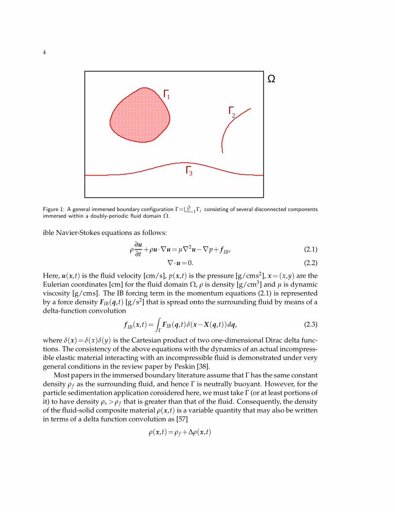
Suppose that a moving elastic solid body Γ is contained within a fluid domain Ω

as pictured in Figure 1. In general, Γ may consist of several disconnected components,Γ=

⋃i Γi, where each Γi can be a one-dimensional elastic membrane (parameterized by a

single real parameter s) or an elastic solid region (whose specification requires two pa-rameters, r and s). We denote the location or “configuration” of the immersed boundaryby X(q,t) [cm], where q is a dimensionless IB parameterization that is used to representeither a scalar s or a vector (r,s), depending on the context. For simplicity, we assumethat Ω=[0,Lx]×[0,Ly] is rectangular in shape and that periodic boundary conditions areapplied in both the x- and y-directions.

The effect of the elastic body on the fluid is to impose a force f IB [g/cm2s2] onto theadjacent fluid particle at location x=X(q,t), which is incorporated into the incompress-

4

1

Γ2

Γ3

ΩΓ

Figure 1: A general immersed boundary configuration Γ=⋃3

i=1 Γi consisting of several disconnected componentsimmersed within a doubly-periodic fluid domain Ω.

ible Navier-Stokes equations as follows:

ρ∂u

∂t+ρu·∇u=µ∇2u−∇p+ f IB, (2.1)

∇·u=0. (2.2)

Here, u(x,t) is the fluid velocity [cm/s], p(x,t) is the pressure [g/cms2], x=(x,y) are theEulerian coordinates [cm] for the fluid domain Ω, ρ is density [g/cm3] and µ is dynamicviscosity [g/cms]. The IB forcing term in the momentum equations (2.1) is representedby a force density FIB(q,t) [g/s2] that is spread onto the surrounding fluid by means of adelta-function convolution

f IB(x,t)=∫

ΓFIB(q,t)δ(x−X(q,t))dq, (2.3)

where δ(x)=δ(x)δ(y) is the Cartesian product of two one-dimensional Dirac delta func-tions. The consistency of the above equations with the dynamics of an actual incompress-ible elastic material interacting with an incompressible fluid is demonstrated under verygeneral conditions in the review paper by Peskin [38].

Most papers in the immersed boundary literature assume that Γ has the same constantdensity ρ f as the surrounding fluid, and hence Γ is neutrally buoyant. However, for theparticle sedimentation application considered here, we must take Γ (or at least portions ofit) to have density ρs >ρ f that is greater than that of the fluid. Consequently, the densityof the fluid-solid composite material ρ(x,t) is a variable quantity that may also be writtenin terms of a delta function convolution as [57]

ρ(x,t)=ρ f +∆ρ(x,t)

5

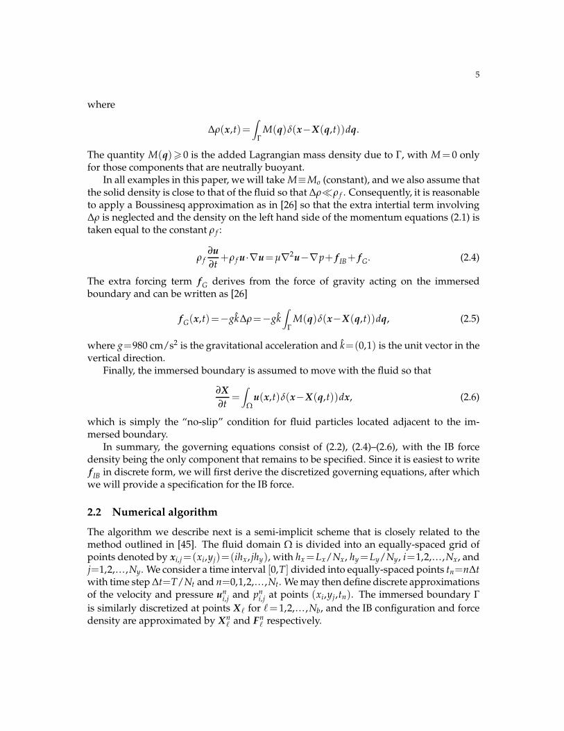
where

∆ρ(x,t)=∫

ΓM(q)δ(x−X(q,t))dq.

The quantity M(q)>0 is the added Lagrangian mass density due to Γ, with M= 0 onlyfor those components that are neutrally buoyant.

In all examples in this paper, we will take M≡Mo (constant), and we also assume thatthe solid density is close to that of the fluid so that ∆ρ≪ρ f . Consequently, it is reasonableto apply a Boussinesq approximation as in [26] so that the extra intertial term involving∆ρ is neglected and the density on the left hand side of the momentum equations (2.1) istaken equal to the constant ρ f :

ρ f∂u

∂t+ρ f u·∇u=µ∇2u−∇p+ f IB+ fG. (2.4)

The extra forcing term fG derives from the force of gravity acting on the immersedboundary and can be written as [26]

fG(x,t)=−gk∆ρ=−gk∫

ΓM(q)δ(x−X(q,t))dq, (2.5)

where g=980 cm/s2 is the gravitational acceleration and k=(0,1) is the unit vector in thevertical direction.

Finally, the immersed boundary is assumed to move with the fluid so that

∂X

∂t=

∫

Ωu(x,t)δ(x−X(q,t))dx, (2.6)

which is simply the “no-slip” condition for fluid particles located adjacent to the im-mersed boundary.

In summary, the governing equations consist of (2.2), (2.4)–(2.6), with the IB forcedensity being the only component that remains to be specified. Since it is easiest to writef IB in discrete form, we will first derive the discretized governing equations, after whichwe will provide a specification for the IB force.

2.2 Numerical algorithm

The algorithm we describe next is a semi-implicit scheme that is closely related to themethod outlined in [45]. The fluid domain Ω is divided into an equally-spaced grid ofpoints denoted by xi,j=(xi,yj)=(ihx, jhy), with hx=Lx/Nx, hy=Ly/Ny, i=1,2,.. . ,Nx, andj=1,2,.. . ,Ny. We consider a time interval [0,T] divided into equally-spaced points tn=n∆twith time step ∆t=T/Nt and n=0,1,2,.. . ,Nt. We may then define discrete approximationsof the velocity and pressure un

i,j and pni,j at points (xi,yj,tn). The immersed boundary Γ

is similarly discretized at points Xℓ for ℓ=1,2,.. . ,Nb, and the IB configuration and forcedensity are approximated by Xn

ℓand Fn

ℓrespectively.

6

Using the above notation, we introduce finite difference operators that approximatethe spatial derivatives appearing in the governing equations. In particular, we define twoone-sided difference approximations of the x–derivative of a grid quantity wi,j

D+x wi,j=

wi+1,j−wi,j

hxand D−

x wi,j=wi,j−wi−1,j

hx, (2.7)

as well as the centered approximation

D0xwi,j=

wi+1,j−wi−1,j

2hx. (2.8)

Analogous definitions apply for the y–derivative approximations D+y , D−

y and D0y, and

the gradient is replaced by the centered approximation ∇h =(D0x,D0

y). Finally, the deltafunction appearing in the integral terms is replaced by the regularized function

δh(x)=1

hxhyφ

(x

hx

)φ

(y

hy

), (2.9)

where

φ(r)=

1

4

(1+cos

(πr

2

)), if |r|62,

0, otherwise.(2.10)

We are now prepared to state the immersed boundary algorithm. In any given timestep, we assume that values of the velocity un−1

i,j and IB configuration Xn−1ℓ

are known

from the previous step. These quantities are evolved to time tn using the following pro-cedure:

1. Compute the IB force density Fn−1IB,ℓ based on the configuration Xn−1

ℓas described in

section 2.3.

2. Spread the IB force to the fluid grid points using a discretization of the integral in(2.3)

f n−1IB,i,j=

Nb

∑ℓ=1

Fn−1IB,ℓ δh(xi,j−Xn−1

ℓ)Ab, (2.11)

and a similar approximation of the integral in (2.5) yields a formula for f n−1G,i,j . The

scaling factor Ab in both cases is inversely proportional to the number of IB points(Nb) and has a different interpretation depending on whether the immersed bound-ary is a 1D fiber (channel wall) or a 2D solid block (circular particle). In the case ofa fiber Ab is a length, while for a solid region Ab is an area; in both cases, the factorAb ensures that the formula (2.11) scales properly with the number of IB points andthat it is a consistent approximation of the corresponding integral. More details onthe precise form of (2.11) and the specification of Ab are provided in section 2.3.

7

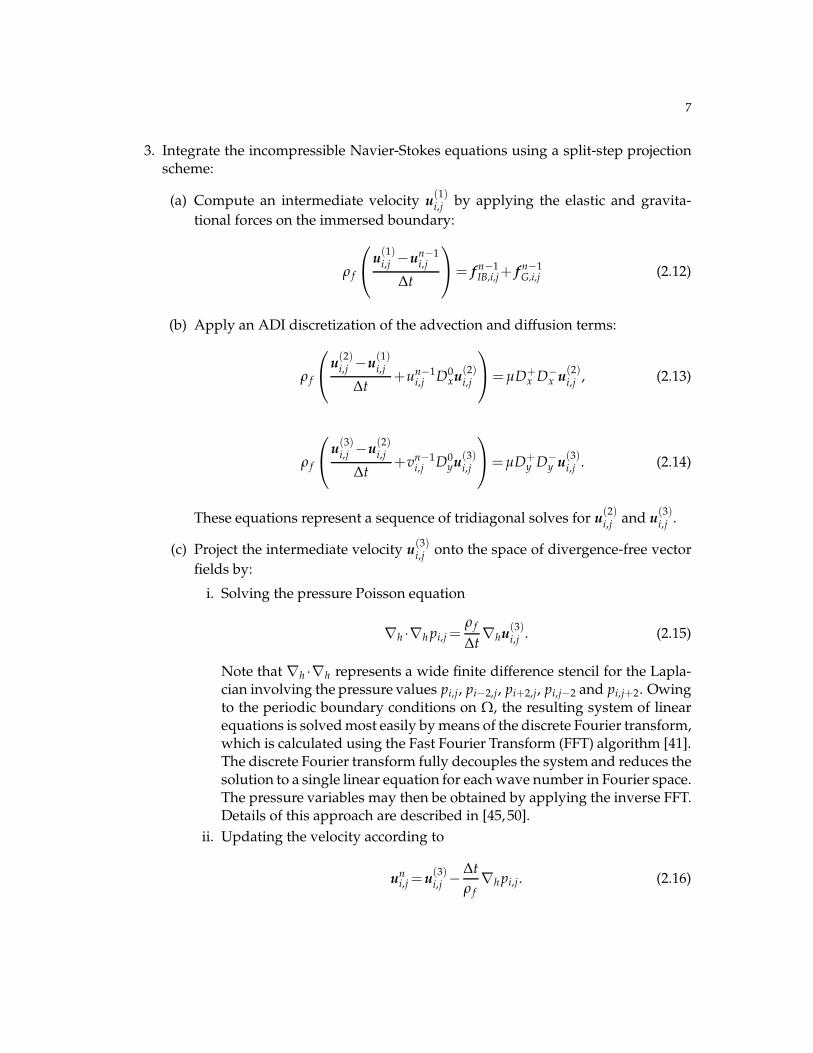
3. Integrate the incompressible Navier-Stokes equations using a split-step projectionscheme:

(a) Compute an intermediate velocity u(1)i,j by applying the elastic and gravita-

tional forces on the immersed boundary:

ρ f

u

(1)i,j −un−1

i,j

∆t

= f n−1

IB,i,j+ f n−1G,i,j (2.12)

(b) Apply an ADI discretization of the advection and diffusion terms:

ρ f

u

(2)i,j −u

(1)i,j

∆t+un−1

i,j D0xu

(2)i,j

=µD+

x D−x u

(2)i,j , (2.13)

ρ f

u

(3)i,j −u

(2)i,j

∆t+vn−1

i,j D0yu

(3)i,j

=µD+

y D−y u

(3)i,j . (2.14)

These equations represent a sequence of tridiagonal solves for u(2)i,j and u

(3)i,j .

(c) Project the intermediate velocity u(3)i,j onto the space of divergence-free vector

fields by:

i. Solving the pressure Poisson equation

∇h ·∇h pi,j =ρ f

∆t∇hu

(3)i,j . (2.15)

Note that ∇h ·∇h represents a wide finite difference stencil for the Lapla-cian involving the pressure values pi,j, pi−2,j, pi+2,j, pi,j−2 and pi,j+2. Owingto the periodic boundary conditions on Ω, the resulting system of linearequations is solved most easily by means of the discrete Fourier transform,which is calculated using the Fast Fourier Transform (FFT) algorithm [41].The discrete Fourier transform fully decouples the system and reduces thesolution to a single linear equation for each wave number in Fourier space.The pressure variables may then be obtained by applying the inverse FFT.Details of this approach are described in [45, 50].

ii. Updating the velocity according to

uni,j =u

(3)i,j −

∆t

ρ f∇h pi,j. (2.16)

8

4. Evolve the immersed boundary using

Xnℓ=Xn−1

ℓ+∆t∑

i,j

uni,j δh(xi,j−Xn−1

ℓ)hxhy. (2.17)

This simple semi-implicit time discretization described above introduces a CFL-like time-step restriction on the numerical scheme that depends on the Reynolds number as wellas the elastic IB force. The dependence of the stable time step on parameters can becharacterized in certain idealized cases [6,27,33], and these results can be used as a guideto selecting a value for ∆t, but in practical computations the time step must be determinedmanually.

This algorithm yields a solution that is first-order accurate in time, and although allspatial derivatives are approximated using second-order finite differences, the methodis also first-order accurate in space owing to errors in velocity interpolation near the im-mersed boundary that arise from the use of the regularized delta function. It is straight-forward to increase the temporal accuracy to second order using an algorithm such asthat proposed by Lai and Peskin [34], but it is much more difficult to increase the spatialaccuracy [21]. Since the focus of the current study is to validate the general IB approachin the study of particle sedimentation, we have chosen to employ the simple schemeabove, and leave for future work the implementation of higher order extensions to thealgorithm.

2.3 Discrete IB force density for particle and channel walls

We begin by describing the geometry for the particle sedimentation problem. Referringto Figure 2, we take a rectangular fluid domain of size Lx×Ly and place two vertical im-mersed fibers representing the channel walls a distance W<Lx apart, symmetric relativeto the channel centerline, and separated from the domain boundary by a narrow strip offluid. With periodic boundary conditions applied on all sides of the domain, the channelwalls naturally connect to each other across the top and bottom boundaries. A single,solid, circular particle of diameter D is initially located at the center of the channel. Lateron, we will consider other initial configurations with one and two particles, but for nowthis will suffice to illustrate the calculation of the IB force density. This circular particle in2D may be thought of as corresponding in 3D to a cross-section of a solid cylinder withinfinite length.

In our sedimentation model, the IB force density FIB is the sum of two terms, FIB =Fw+Fc, where Fw represents the force density generated by the channel walls and Fc isthat generated by the circular particle. These forces are discussed separately in the nexttwo sections.

2.3.1 Elastic force from the channel walls, Fw

The vertical walls are discretized using an equally-spaced array of IB points that are ini-

tially at locations Xw,Lℓ

=(

12(Lx−W),ℓhw

)for the left wall, and Xw,R

ℓ=(

12(Lx+W),ℓhw

)

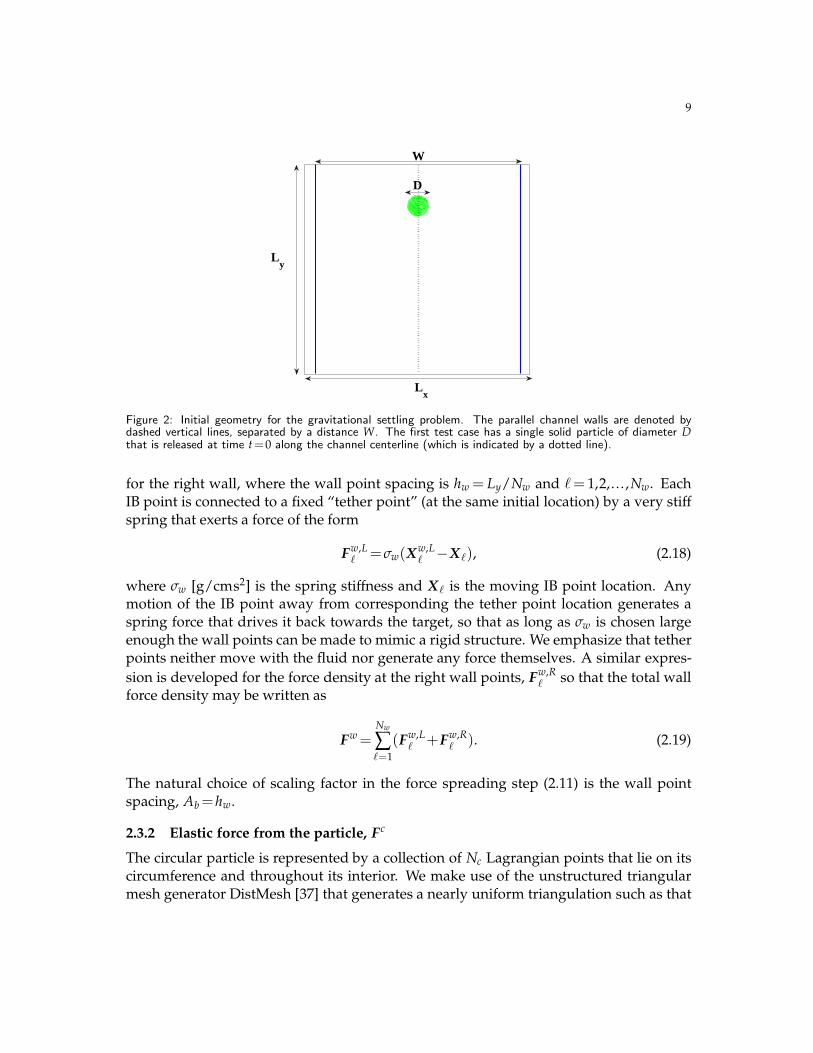
9

D

W

Lx

Ly

Figure 2: Initial geometry for the gravitational settling problem. The parallel channel walls are denoted bydashed vertical lines, separated by a distance W. The first test case has a single solid particle of diameter Dthat is released at time t=0 along the channel centerline (which is indicated by a dotted line).

for the right wall, where the wall point spacing is hw = Ly/Nw and ℓ= 1,2,.. . ,Nw. EachIB point is connected to a fixed “tether point” (at the same initial location) by a very stiffspring that exerts a force of the form

Fw,Lℓ

=σw(Xw,Lℓ

−Xℓ), (2.18)

where σw [g/cms2] is the spring stiffness and Xℓ is the moving IB point location. Anymotion of the IB point away from corresponding the tether point location generates aspring force that drives it back towards the target, so that as long as σw is chosen largeenough the wall points can be made to mimic a rigid structure. We emphasize that tetherpoints neither move with the fluid nor generate any force themselves. A similar expres-

sion is developed for the force density at the right wall points, Fw,Rℓ

so that the total wallforce density may be written as

Fw =Nw

∑ℓ=1

(Fw,Lℓ

+Fw,Rℓ

). (2.19)

The natural choice of scaling factor in the force spreading step (2.11) is the wall pointspacing, Ab=hw.

2.3.2 Elastic force from the particle, Fc

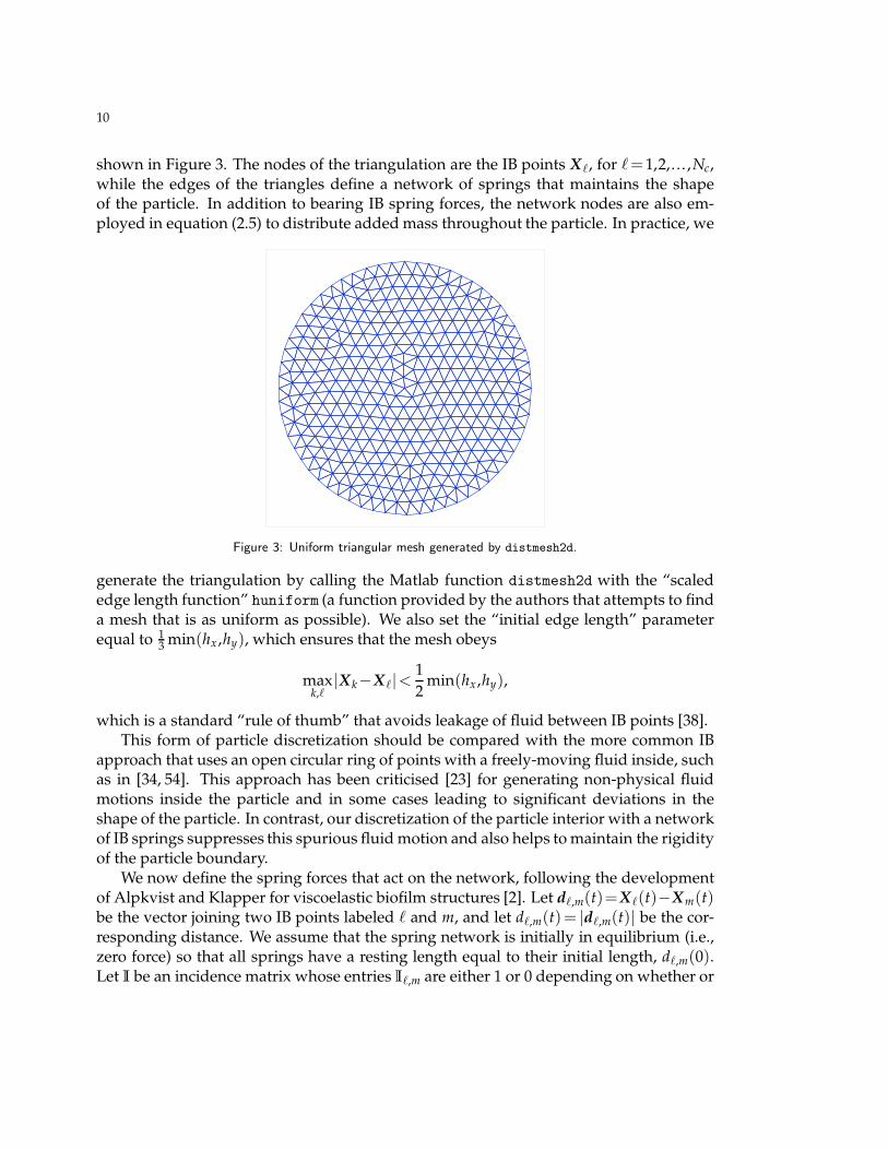
The circular particle is represented by a collection of Nc Lagrangian points that lie on itscircumference and throughout its interior. We make use of the unstructured triangularmesh generator DistMesh [37] that generates a nearly uniform triangulation such as that

10

shown in Figure 3. The nodes of the triangulation are the IB points Xℓ, for ℓ=1,2,.. . ,Nc,while the edges of the triangles define a network of springs that maintains the shapeof the particle. In addition to bearing IB spring forces, the network nodes are also em-ployed in equation (2.5) to distribute added mass throughout the particle. In practice, we

Figure 3: Uniform triangular mesh generated by distmesh2d.

generate the triangulation by calling the Matlab function distmesh2d with the “scalededge length function” huniform (a function provided by the authors that attempts to finda mesh that is as uniform as possible). We also set the “initial edge length” parameterequal to 1

3 min(hx,hy), which ensures that the mesh obeys

maxk,ℓ

|Xk−Xℓ|<1

2min(hx,hy),

which is a standard “rule of thumb” that avoids leakage of fluid between IB points [38].This form of particle discretization should be compared with the more common IB

approach that uses an open circular ring of points with a freely-moving fluid inside, suchas in [34, 54]. This approach has been criticised [23] for generating non-physical fluidmotions inside the particle and in some cases leading to significant deviations in theshape of the particle. In contrast, our discretization of the particle interior with a networkof IB springs suppresses this spurious fluid motion and also helps to maintain the rigidityof the particle boundary.

We now define the spring forces that act on the network, following the developmentof Alpkvist and Klapper for viscoelastic biofilm structures [2]. Let dℓ,m(t)=Xℓ(t)−Xm(t)be the vector joining two IB points labeled ℓ and m, and let dℓ,m(t)= |dℓ,m(t)| be the cor-responding distance. We assume that the spring network is initially in equilibrium (i.e.,zero force) so that all springs have a resting length equal to their initial length, dℓ,m(0).Let I be an incidence matrix whose entries Iℓ,m are either 1 or 0 depending on whether or

11

not points ℓ and m are connected, respectively. Then the force density acting on the ℓth IBpoint in the network is

Fcℓ=σc

Nb

∑m=1

Iℓ,m 6=0

Iℓ,mdℓ,m

dℓ,m(dℓ,m(0)−dℓ,m), (2.20)

where the sum is taken only over those m for which Xm is connected to Xℓ in the network.We have also assumed that the spring stiffness σc [g/cms2] is constant for all networkconnections. The total elastic force density generated by all IB points making up thecircular particle is then given by

Fc=Nc

∑ℓ=1

Fcℓ. (2.21)

The appropriate scaling factor for the force integral (2.11) is the average area of a trian-gular mesh cell, Ab =π(D/2)2/Nc. A similar approach was employed by Hopkins andFauci [26] to simulate a suspension of microbial cells that they treated as point particles.

3 Approximate formulas for settling velocity

We next review some of the existing analytical and experimental results on the settling ofa single particle falling under the action of gravity. The study of a spherical particle in anunbounded fluid medium in 3D is a classical problem that was considered by Stokes [47],who obtained a formula for the settling velocity that is now known as Stokes’ law. Wewill first state Stokes’ result and then modify it for a circular particle in 2D, which corre-sponds to an idealized “infinite cylinder” in 3D. We then consider the case of a circularparticle falling in a bounded fluid domain between two vertical walls and then reviewseveral of the most commonly-used formulas for the “wall-correction factors” that havebeen obtained from either fitting to experimental data or using approximate analyticaltechniques. A fairly extensive overview of settling for cylindrical particles, includingmany of the wall correction formulas reported in the literature, is given by Champmartinand Ambari [11].

3.1 Stokes’ law for a spherical particle in 3D

There are two main forces acting upon a massive particle settling in a fluid: the gravita-tional force Fg, and the drag force Fd due to the “friction” between the particle and thefluid. A particle that is initially at rest will accelerate under the action of gravity, and asthe particle begins to move through the fluid it experiences a drag force in the directionopposite to its motion that increases with the speed of the particle relative to the fluid.If the drag force becomes large enough that it equals the gravitational force, then the

12

two forces are in balance and no further acceleration occurs. The particle velocity in thisequilibrium state is known as the settling or terminal velocity.

We take a sphere of diameter D and density ρs whose added mass relative to the fluid

is 43 π

(D2

)3(ρs−ρ f ). The net gravitational force acting on the sphere is

Fg=4π

3

(D

2

)3

g(ρs−ρ f ), (3.1)

and the corresponding drag force is

Fd=1

2Cdρ f V

2π

(D

2

)2

, (3.2)

where Cd is the drag coefficient for a sphere and V is the velocity of the sphere relativeto the fluid. The settling velocity Vs corresponds to the long-term steady state in whichdrag and gravity forces are in balance, so that Fd=Fg. By equating (3.1) and (3.2), we cansolve for

Vs =

√4gD(ρs−ρ f )

3Cdρ f, (3.3)

keeping in mind that the drag coefficient on the right hand side also typically depends onthe settling velocity, Vs. Indeed, we know from [3] that the drag coefficient for a spherecan be approximated for small Reynolds number by

Cd=24

Re=

24µ

ρ f VsD, (3.4)

where we have taken

Re=ρ f DVs

µ, (3.5)

based on the particle diameter. Substituting this expression into (3.3) and solving for Vs

we obtain Stokes’ law

Vs=gD2(ρs−ρ f )

18µ, (3.6)

which is valid for Re.0.1.

3.2 Settling velocity for a circular particle in 2D

A similar argument may be used to derive the corresponding expression for a circularparticle in 2D. We begin by considering a cylinder with diameter D and length ℓ and take

13

the limit as ℓ→ ∞ in order to obtain a result that is relevant to our 2D geometry. The

immersed cylinder has an added mass (relative to the fluid) of m=π(

D2

)2ℓ(ρs−ρ f ) for

which the net gravitational force is

Fg=π

4gℓD2(ρs−ρ f ), (3.7)

and the drag force is

Fd=1

2Cdρ f V

2Dℓ. (3.8)

Notice that the cross-sectional area factor π(D/2)2 for the sphere from (3.2) is replacedby Dℓ for the cylinder, and the tildes are used here to denote cylindrical quantities. Wealso make use of the drag coefficient for a cylinder from [3]

Cd=8π

Re ln(

7.4Re

) , (3.9)

which holds when Re≪1.The settling velocity for the cylinder is then obtained by equating the gravitational

and drag forces in (3.7) and (3.8), which yields

Vs =

√πgD(ρs−ρ f )

2Cdρ f

. (3.10)

Observe that the factor of length ℓ cancels in the above expression, so that this sameexpression is valid also for the 2D geometry in the ℓ→∞ limit. Furthermore, this expres-sion is the same as that for the sphere in (3.3) except that the factor

√4/3 is replaced here

with√

π/2, and of course the cylinder drag coefficient is also different. When equations(3.9)–(3.10) are taken together, they reduce to a nonlinear equation in Re

f (Re)=Re− ρ f gD3(ρs−ρ f )

16µ2ln

(7.4

Re

)=0, (3.11)

which can alternatively be written as an equation in Vs. It is easy to show that the functionf (x) is continuous on the interval 0< x<∞ and has the following properties:

limx→0+

f (x)=−∞, limx→∞

f (x)=+∞ and f ′(x)>0.

Therefore, f is guaranteed to have a unique positive real root by the intermediate valuetheorem.

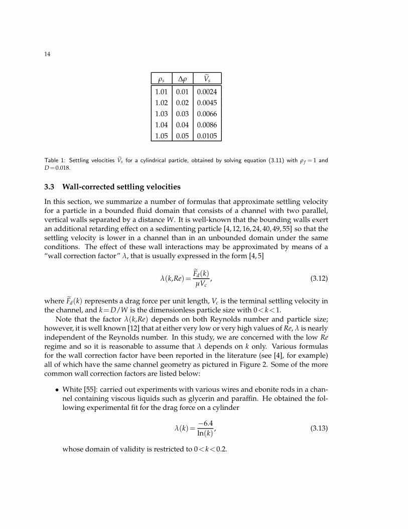
Newton’s method may be used to solve (3.11) for Re, and we find that any initial guessfor Re suffices since the convergence is to rapid. Table 1 lists values of Vs from (3.11) forparameters D=0.018 and ρs ranging from 1.01 to 1.05. As expected, the settling velocityincreases with particle density as in the Stokes case.

14

ρs ∆ρ Vs

1.01 0.01 0.0024

1.02 0.02 0.0045

1.03 0.03 0.0066

1.04 0.04 0.0086

1.05 0.05 0.0105

Table 1: Settling velocities Vs for a cylindrical particle, obtained by solving equation (3.11) with ρ f = 1 and

D=0.018.

3.3 Wall-corrected settling velocities

In this section, we summarize a number of formulas that approximate settling velocityfor a particle in a bounded fluid domain that consists of a channel with two parallel,vertical walls separated by a distance W. It is well-known that the bounding walls exertan additional retarding effect on a sedimenting particle [4, 12, 16, 24, 40, 49, 55] so that thesettling velocity is lower in a channel than in an unbounded domain under the sameconditions. The effect of these wall interactions may be approximated by means of a“wall correction factor” λ, that is usually expressed in the form [4, 5]

λ(k,Re)=Fd(k)

µVc, (3.12)

where Fd(k) represents a drag force per unit length, Vc is the terminal settling velocity inthe channel, and k=D/W is the dimensionless particle size with 0< k<1.

Note that the factor λ(k,Re) depends on both Reynolds number and particle size;however, it is well known [12] that at either very low or very high values of Re, λ is nearlyindependent of the Reynolds number. In this study, we are concerned with the low Reregime and so it is reasonable to assume that λ depends on k only. Various formulasfor the wall correction factor have been reported in the literature (see [4], for example)all of which have the same channel geometry as pictured in Figure 2. Some of the morecommon wall correction factors are listed below:

• White [55]: carried out experiments with various wires and ebonite rods in a chan-nel containing viscous liquids such as glycerin and paraffin. He obtained the fol-lowing experimental fit for the drag force on a cylinder

λ(k)=−6.4

ln(k), (3.13)

whose domain of validity is restricted to 0< k<0.2.

15

• Faxen [16, 24]: derived an approximate analytical solution of the Stokes equations,from which he obtained

λ(k)=−4π

0.9157+ln(k)−1.724k2+1.730k4−2.406k6+4.591k8. (3.14)

Some authors claim that this approximation is valid for k as large as 0.5 [4], whileothers cite an upper bound of k=0.3 or even lower [40] which is more in line withour numerical simulations (see Figure 8 in Section 4).

• Takaisi [49]: used an analytical solution of Oseen’s equations to obtain the approx-imation

λ(k)=−4π

0.9156+ln(k), (3.15)

which is restricted to 0 < k < 0.2. He also performed a comparison with White’sexperimental fit and showed that the two expressions match reasonably well whenk<0.05.

If we now consider λ(k) to be a known function of the dimensionless particle size k,then equation (3.12) can be solved for the drag force per unit length as

Fd(k)=Vcµλ(k).

Equating this expression with the gravitational force

Fg=π

4gD2(ρs−ρ f ),

we find the following formula for the confined (or wall-corrected) terminal settling ve-locity of a cylinder

Vc=πgD2(ρs−ρ f )

4µλ(k). (3.16)

In the next section, this expression will be compared with numerically simulated valuesfor the three choices of λ(k) listed above.

4 Numerical results: Single particle case

In this section, we concentrate on a single particle that settles under the influence ofgravity. Two initial configurations are investigated: one a symmetric case in which theparticle is released along the centerline, and a second asymmetric case where the particleis released from an off-center location.

16

We restrict ourselves to a low Reynolds number regime corresponding to Re.7, whereRe refers to a “final” Reynolds number that is based on the vertical velocity after a par-ticle has achieved its terminal settling velocity. Unless otherwise indicated, we choosephysical parameters ρ f = 1, ρs = 1.01 and D= 0.08. The wall and particle IB spring stiff-ness values are taken large enough that the walls and particle boundary do not deform“too much” from their initial shapes – taking σw =σc =3×104 keeps the relative error inthese boundary shapes to within approximately 0.2%.

Except for the convergence study in the next section, most of our simulations areperformed at the same grid resolution of hx = hy = 0.0083 and with a time step of ∆t =10−5. We also select the number of IB points for the two channel walls (Nw) such that theratio of spacing between wall points to fluid grid size is hw/min(hx,hy)≈ 1

3 – this ratio

is well within the factor of 12 that is recommended to avoid leakage of fluid between IB

points [38]. We also adjust the number of IB points for the particle (Nc) until the initialmesh computed by DistMesh satisfies the same criterion.

4.1 Convergence study

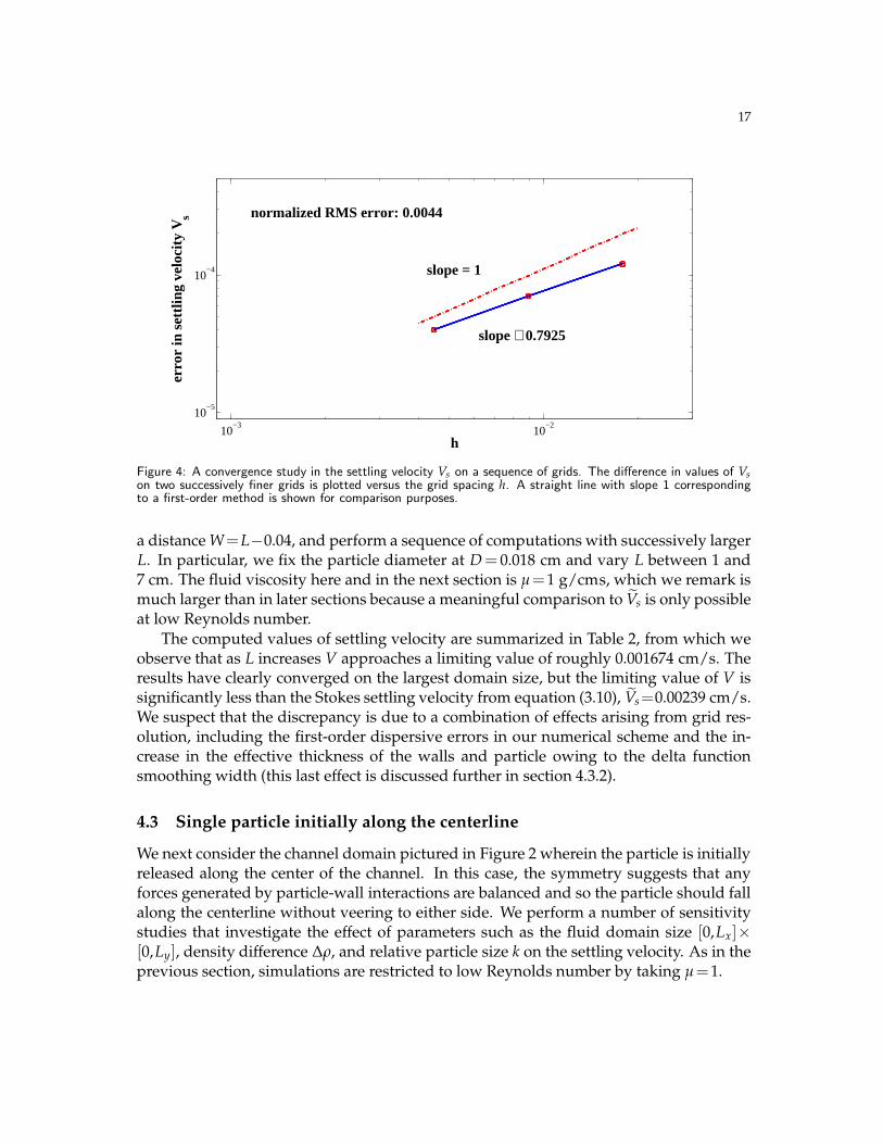
We begin by performing a convergence study that validates the spatial accuracy of ournumerical method. As mentioned earlier in section 2.2, the IB algorithm being employedhere is well-known to be first order accurate in space. To verify this result, we select asequence of fluid grids with Nx = Ny = 56, 112, 224 and 448 on a square domain withside length Lx = Ly = 1, and use the settling velocity Vs as a representative measure ofthe solution for each case. The difference between values of Vs on successive grids iscalculated and the results are plotted in Figure 4, which demonstrates that our numericalsolution converges as the grid spacing is reduced. The curve is nearly a straight line ona log-log scale, and the slope of 0.79 obtained from a least squares fit suggests that ourimplementation of the IB method is close to the expected first-order accuracy. Similarconvergence rates are observed for other quantities such as fluid velocity, IB position, etc.

4.2 Comparison with Stokes’ law

We aim next to validate the numerical method against the settling velocity Vs for a cylin-der in an unbounded medium. However, we recall that our doubly periodic geometryimplies that a single particle actually corresponds to an infinite array of sedimentingparticles. Therefore, in the absence of solid boundaries or any other mechanism for dis-sipating energy, the net effect of gravity acting on such an infinite array of mass-bearingparticles will be to accelerate the particles and the surrounding fluid indefinitely. Thissituation is clearly non-physical, and so instead we introduce walls into the domain thatare situated “far enough” from the particle so as to minimize wall-particle interactionsand yet still permit the particle to reach its natural terminal velocity. To this end, we takea square domain with side length Lx=Ly=L that contains two vertical walls separated by

17

10−3

10−2

10−5

10−4

h

erro

r in

set

tling

vel

ocity

Vs

slope ≅ 0.7925

normalized RMS error: 0.0044

slope = 1

Figure 4: A convergence study in the settling velocity Vs on a sequence of grids. The difference in values of Vson two successively finer grids is plotted versus the grid spacing h. A straight line with slope 1 correspondingto a first-order method is shown for comparison purposes.

a distance W=L−0.04, and perform a sequence of computations with successively largerL. In particular, we fix the particle diameter at D= 0.018 cm and vary L between 1 and7 cm. The fluid viscosity here and in the next section is µ=1 g/cms, which we remark ismuch larger than in later sections because a meaningful comparison to Vs is only possibleat low Reynolds number.

The computed values of settling velocity are summarized in Table 2, from which weobserve that as L increases V approaches a limiting value of roughly 0.001674 cm/s. Theresults have clearly converged on the largest domain size, but the limiting value of V issignificantly less than the Stokes settling velocity from equation (3.10), Vs=0.00239 cm/s.We suspect that the discrepancy is due to a combination of effects arising from grid res-olution, including the first-order dispersive errors in our numerical scheme and the in-crease in the effective thickness of the walls and particle owing to the delta functionsmoothing width (this last effect is discussed further in section 4.3.2).

4.3 Single particle initially along the centerline

We next consider the channel domain pictured in Figure 2 wherein the particle is initiallyreleased along the center of the channel. In this case, the symmetry suggests that anyforces generated by particle-wall interactions are balanced and so the particle should fallalong the centerline without veering to either side. We perform a number of sensitivitystudies that investigate the effect of parameters such as the fluid domain size [0,Lx]×[0,Ly], density difference ∆ρ, and relative particle size k on the settling velocity. As in theprevious section, simulations are restricted to low Reynolds number by taking µ=1.

18

L computed V

1 0.001230

2 0.001462

3 0.001565

4 0.001635

5 0.001673

6 0.001674

7 0.001674

Table 2: Computed settling velocity as a function of domain size L for D=0.018.

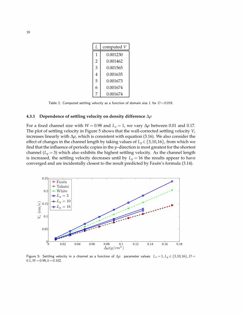
4.3.1 Dependence of settling velocity on density difference ∆ρ

For a fixed channel size with W = 0.98 and Lx = 1, we vary ∆ρ between 0.01 and 0.17.The plot of settling velocity in Figure 5 shows that the wall-corrected settling velocity Vc

increases linearly with ∆ρ, which is consistent with equation (3.16). We also consider theeffect of changes in the channel length by taking values of Ly∈3,10,16, from which wefind that the influence of periodic copies in the y–direction is most greatest for the shortestchannel (Ly = 3) which also exhibits the highest settling velocity. As the channel lengthis increased, the settling velocity decreases until by Ly = 16 the results appear to haveconverged and are incidentally closest to the result predicted by Faxen’s formula (3.14).

0 0.02 0.04 0.06 0.08 0.1 0.12 0.14 0.16 0.180

0.05

0.1

0.15

0.2

0.25

∆ρ(g/cm3 )

Vc

(cm

/s)

FaxenTakaisiWhiteLy = 3

Ly = 10

Ly = 16

Figure 5: Settling velocity in a channel as a function of ∆ρ. parameter values: Lx = 1, Ly ∈ 3,10,16, D =0.1, W=0.98, k=0.102.

19

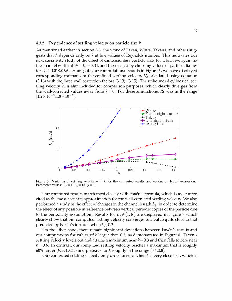
4.3.2 Dependence of settling velocity on particle size k

As mentioned earlier in section 3.3, the work of Faxen, White, Takaisi, and others sug-gests that λ depends only on k at low values of Reynolds number. This motivates ournext sensitivity study of the effect of dimensionless particle size, for which we again fixthe channel width at W=Lx−0.04, and then vary k by choosing values of particle diame-ter D∈ [0.018,0.96]. Alongside our computational results in Figure 6, we have displayedcorresponding estimates of the confined settling velocity Vc calculated using equation(3.16) with the three wall correction factors (3.13)–(3.15). The unbounded cylindrical set-tling velocity Vs is also included for comparison purposes, which clearly diverges fromthe wall-corrected values away from k = 0. For these simulations, Re was in the range[1.2×10−5,1.8×10−2].

0 0.05 0.1 0.15 0.2 0.25 0.3 0.35 0.40

0.05

0.1

k

Vc (

cm/s

)

WhiteFaxen eighth orderTakaisiOur simulationsAnalytical

Figure 6: Variation of settling velocity with k for the computed results and various analytical expressions.Parameter values: Lx =1, Ly=16, µ=1.

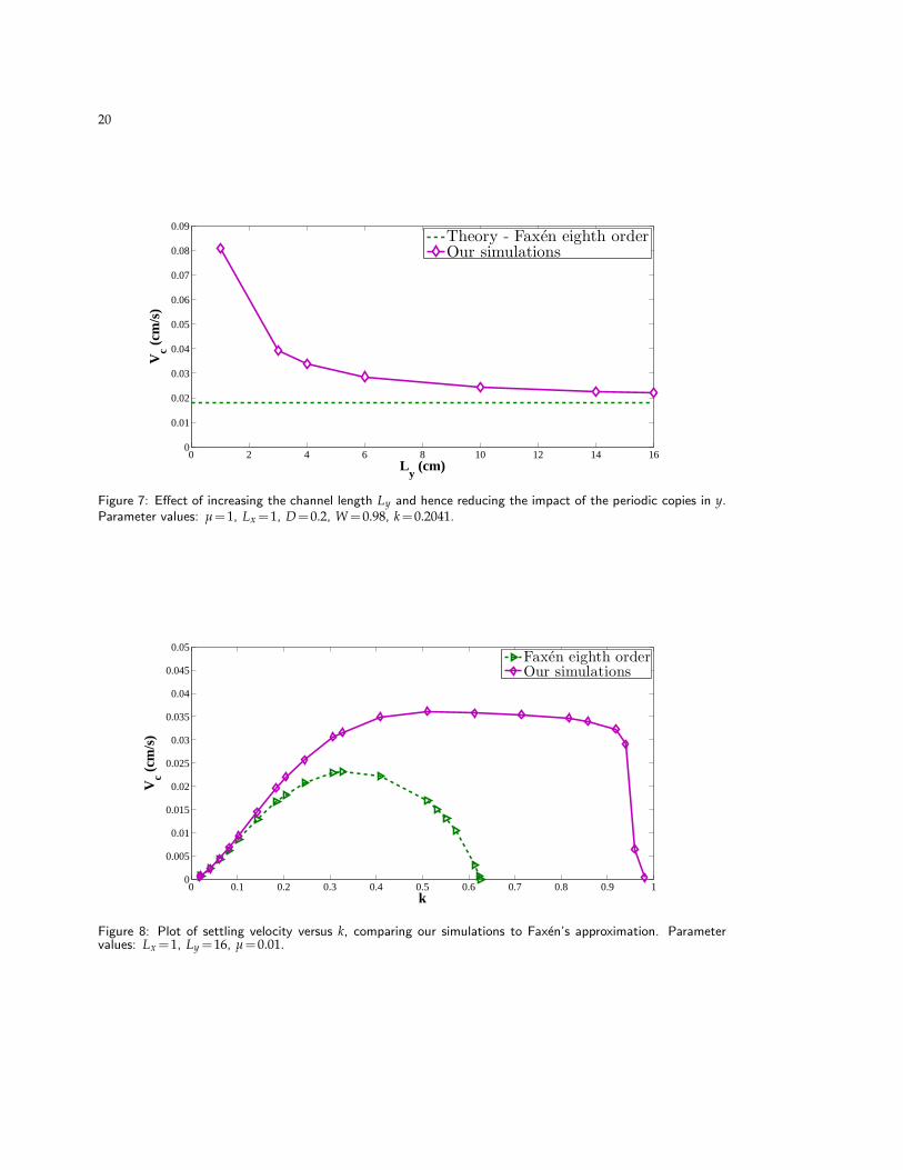
Our computed results match most closely with Faxen’s formula, which is most oftencited as the most accurate approximation for the wall-corrected settling velocity. We alsoperformed a study of the effect of changes in the channel length Ly, in order to determinethe effect of any possible interference between vertical periodic copies of the particle dueto the periodicity assumption. Results for Ly ∈ [1,16] are displayed in Figure 7 whichclearly show that our computed settling velocity converges to a value quite close to thatpredicted by Faxen’s formula when k.0.2.

On the other hand, there remain significant deviations between Faxen’s results andour computations for values of k larger than 0.2, as demonstrated in Figure 8. Faxen’ssettling velocity levels out and attains a maximum near k=0.3 and then falls to zero neark= 0.6. In contrast, our computed settling velocity reaches a maximum that is roughly60% larger (Vc≈0.035) and plateaus for k roughly in the range [0.4,0.8].

Our computed settling velocity only drops to zero when k is very close to 1, which is

20

0 2 4 6 8 10 12 14 160

0.01

0.02

0.03

0.04

0.05

0.06

0.07

0.08

0.09

Ly (cm)

Vc (

cm/s

)

Theory - Faxen eighth orderOur simulations

Figure 7: Effect of increasing the channel length Ly and hence reducing the impact of the periodic copies in y.Parameter values: µ=1, Lx =1, D=0.2, W=0.98, k=0.2041.

0 0.1 0.2 0.3 0.4 0.5 0.6 0.7 0.8 0.9 10

0.005

0.01

0.015

0.02

0.025

0.03

0.035

0.04

0.045

0.05

k

Vc (

cm/s

)

Faxen eighth orderOur simulations

Figure 8: Plot of settling velocity versus k, comparing our simulations to Faxen’s approximation. Parametervalues: Lx =1, Ly =16, µ=0.01.

21

easily justified since the particle must come to a stop as it come into direct contact withthe stationary walls. However, our results in Figure 8 show that Vc actually tends tozero not at k=1 but rather k≈0.96. The reason for this apparent reduction of 0.04 in thechannel width is that the approximate delta function in our numerical scheme has a finitesmoothing width that has the effect of introducing an extra “effective thickness” to boththe walls and the particle. The numerical simulations in [46] show that when using thecosine delta function, the effective thickness of an immersed boundary is approximately1.6h, where h is the fluid grid spacing†. Consequently, a particle with diameter D shouldhave an effective diameter of roughly Deff ≈D+3.2h, while the walls should each extendan additional distance of 3.2h into the channel. Taken together this suggests a total re-duction of 6.4h in the effective channel width, which for h=0.0083 equals approximately0.053. This is not far away from the observed reduction of 0.04.

We summarize the behavior from our numerical simulations as follows:

• For small particle diameters corresponding to k∈ [0,0.2], the particle is far enoughfrom the channel walls that the retarding effects of wall drag are not as prominent.In this range, the dependence of the settling velocity is roughly proportional to k,which is consistent with Faxen’s result.

• For intermediate values of k, roughly in the range [0.4,0.8], the settling velocity hasattained a maximum value and remains approximately constant. For these particlesizes, the interactions with the walls are at long range and are mediated by the fluid.

• For values of k∈ [0.8,1.0], the particle is very close to the walls, giving rise to close-range interactions that slow the particle significantly.

Of course, the validity of Faxen’s approximation is limited to k.0.2 and so it is no surprisethat our results differ so much for larger k.

4.4 Single particle initially off-center

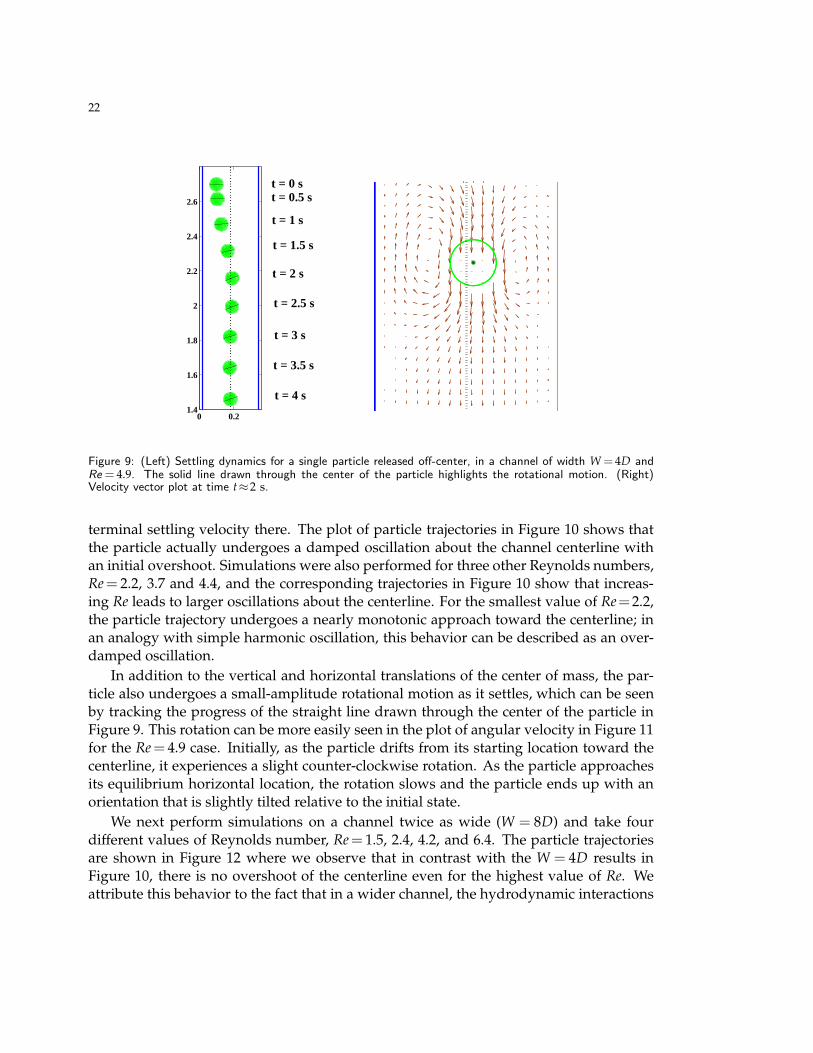
In this section, we consider an asymmetry initial condition in which the particle is re-leased from an off-center location. In Figure 9, the initial configuration labeled “t= 0 s”shows the particle a distance W/2 to the left of center. The diameter of the particle istaken to be D=0.08 cm, the channel length is Ly=3, and we consider two different chan-nel widths, W = 4D and 8D. We also vary Reynolds number by taking values of theviscosity µ∈ [0.006,0.018] g/cms. This choice of parameters allows us to draw a compar-ison with the analytical and experimental results reported by Sucker and Brauer [48], aswell as numerical simulations of Feng et al. [17].

The settling dynamics are pictured in Figure 9 for W=4D and Re=4.9. As the particlefalls, it initially drifts to the right toward the channel centerline, eventually attaining its

†Note that the effective thickness depends on the choice of regularized delta function. Bringley [9] computedan effective thickness closer to 1.25h for a different but closely-related approximate delta function.

22

0 0.21.4

1.6

1.8

2

2.2

2.4

2.6

t = 0 s

t = 2 s

t = 2.5 s

t = 3 s

t = 3.5 s

t = 0.5 s

t = 1 s

t = 1.5 s

t = 4 s

Figure 9: (Left) Settling dynamics for a single particle released off-center, in a channel of width W = 4D andRe = 4.9. The solid line drawn through the center of the particle highlights the rotational motion. (Right)Velocity vector plot at time t≈2 s.

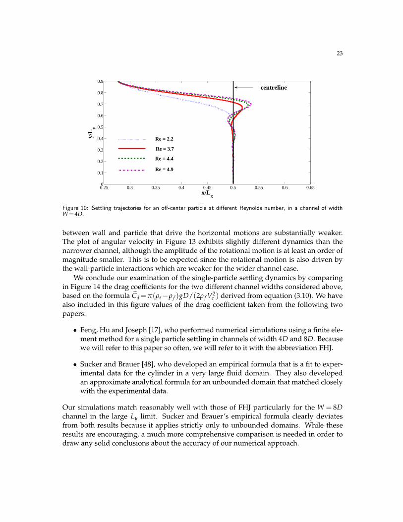
terminal settling velocity there. The plot of particle trajectories in Figure 10 shows thatthe particle actually undergoes a damped oscillation about the channel centerline withan initial overshoot. Simulations were also performed for three other Reynolds numbers,Re= 2.2, 3.7 and 4.4, and the corresponding trajectories in Figure 10 show that increas-ing Re leads to larger oscillations about the centerline. For the smallest value of Re=2.2,the particle trajectory undergoes a nearly monotonic approach toward the centerline; inan analogy with simple harmonic oscillation, this behavior can be described as an over-damped oscillation.

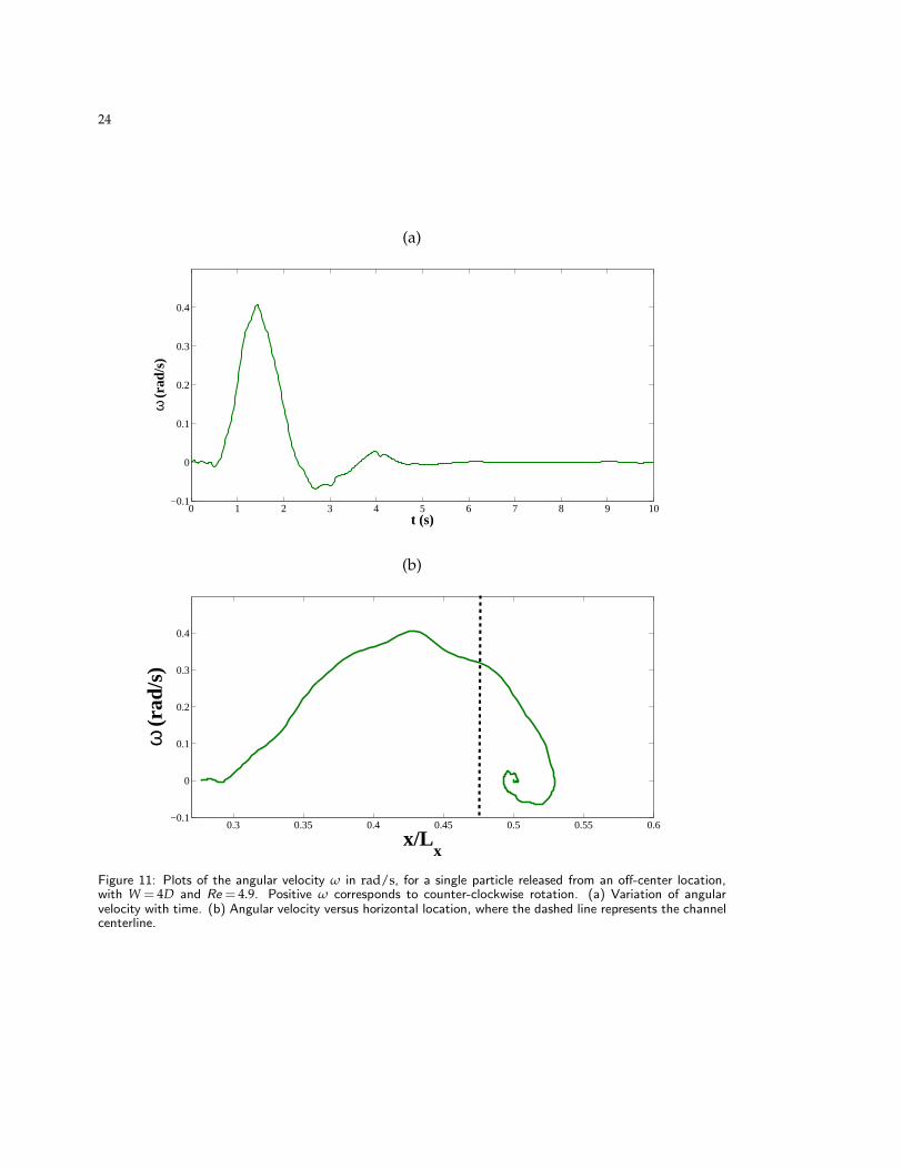
In addition to the vertical and horizontal translations of the center of mass, the par-ticle also undergoes a small-amplitude rotational motion as it settles, which can be seenby tracking the progress of the straight line drawn through the center of the particle inFigure 9. This rotation can be more easily seen in the plot of angular velocity in Figure 11for the Re= 4.9 case. Initially, as the particle drifts from its starting location toward thecenterline, it experiences a slight counter-clockwise rotation. As the particle approachesits equilibrium horizontal location, the rotation slows and the particle ends up with anorientation that is slightly tilted relative to the initial state.

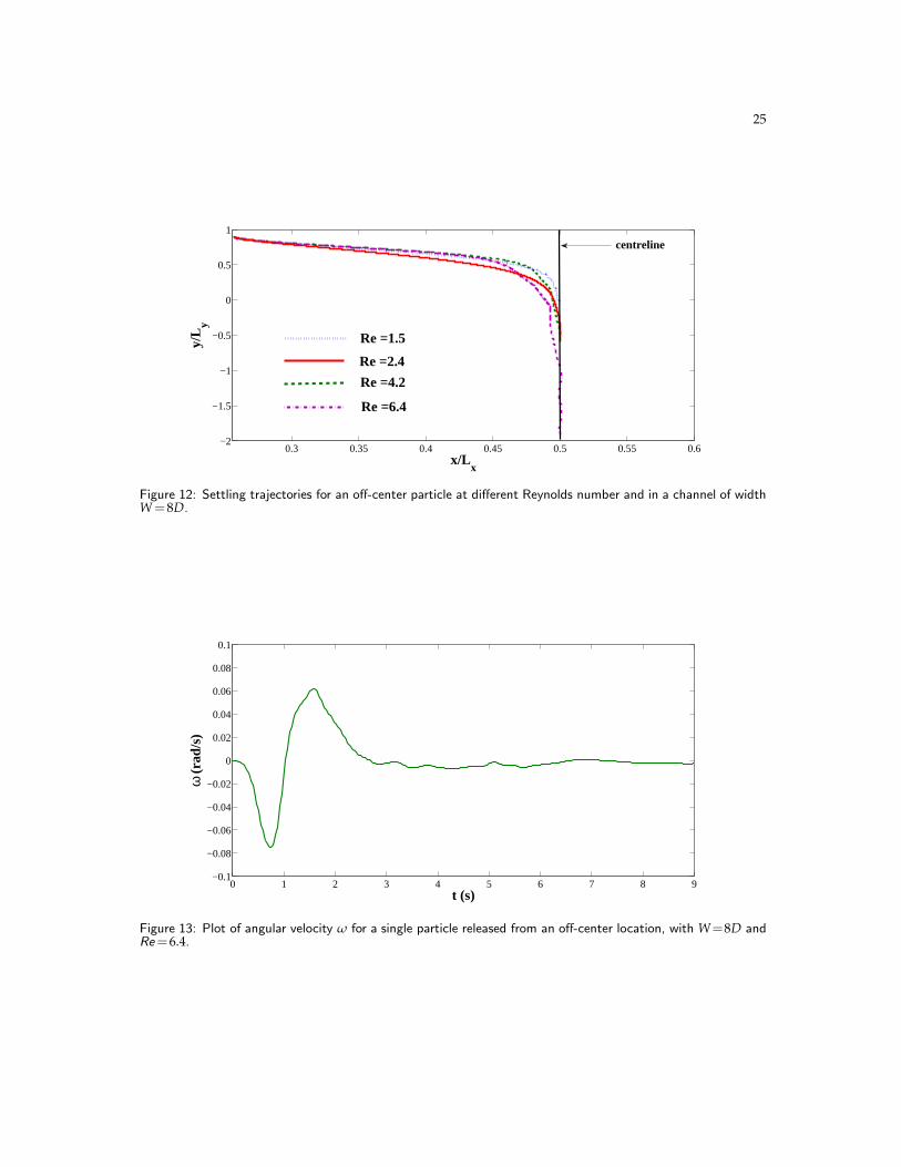
We next perform simulations on a channel twice as wide (W = 8D) and take fourdifferent values of Reynolds number, Re= 1.5, 2.4, 4.2, and 6.4. The particle trajectoriesare shown in Figure 12 where we observe that in contrast with the W = 4D results inFigure 10, there is no overshoot of the centerline even for the highest value of Re. Weattribute this behavior to the fact that in a wider channel, the hydrodynamic interactions

23

0.25 0.3 0.35 0.4 0.45 0.5 0.55 0.6 0.650

0.1

0.2

0.3

0.4

0.5

0.6

0.7

0.8

0.9

x/Lx

y/L

y

Re = 2.2

Re = 3.7

Re = 4.4

Re = 4.9

centreline

Figure 10: Settling trajectories for an off-center particle at different Reynolds number, in a channel of widthW=4D.

between wall and particle that drive the horizontal motions are substantially weaker.The plot of angular velocity in Figure 13 exhibits slightly different dynamics than thenarrower channel, although the amplitude of the rotational motion is at least an order ofmagnitude smaller. This is to be expected since the rotational motion is also driven bythe wall-particle interactions which are weaker for the wider channel case.

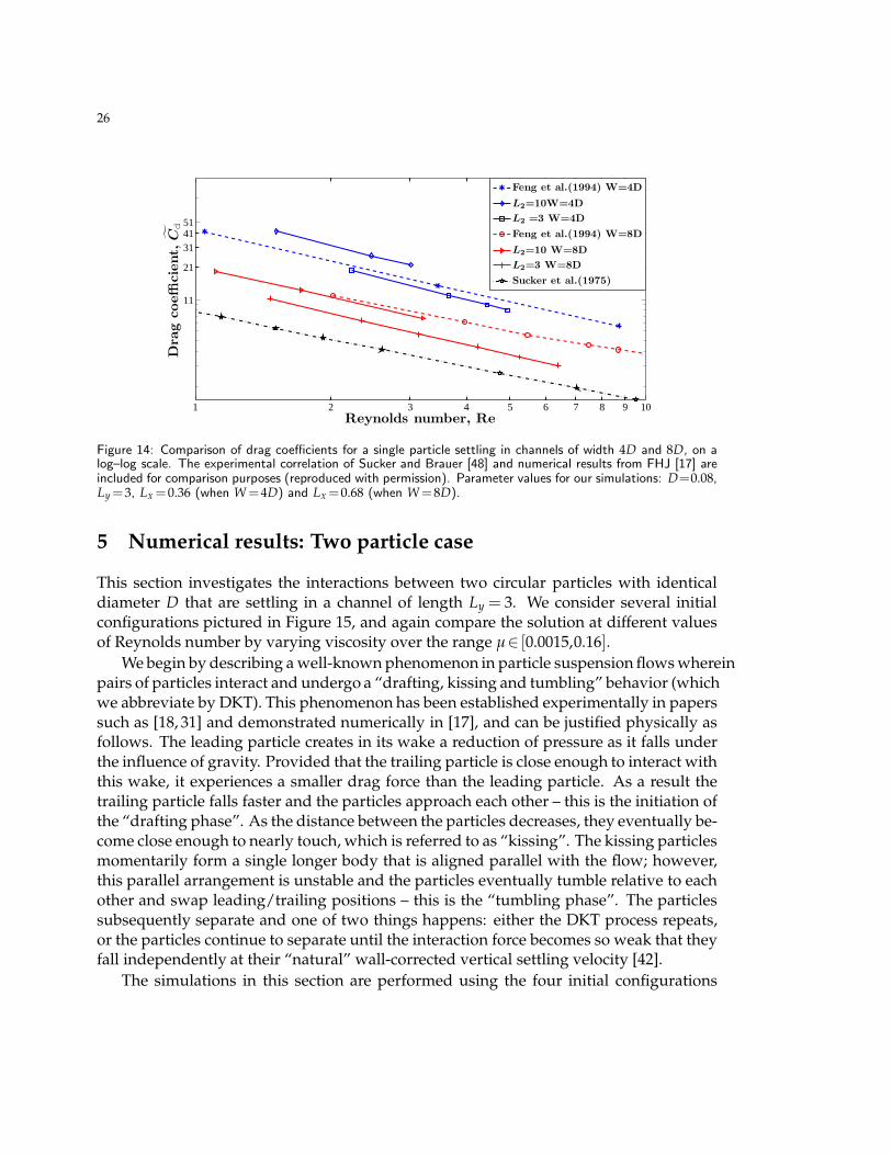
We conclude our examination of the single-particle settling dynamics by comparingin Figure 14 the drag coefficients for the two different channel widths considered above,based on the formula Cd=π(ρs−ρ f )gD/(2ρ f V2

c ) derived from equation (3.10). We havealso included in this figure values of the drag coefficient taken from the following twopapers:

• Feng, Hu and Joseph [17], who performed numerical simulations using a finite ele-ment method for a single particle settling in channels of width 4D and 8D. Becausewe will refer to this paper so often, we will refer to it with the abbreviation FHJ.

• Sucker and Brauer [48], who developed an empirical formula that is a fit to exper-imental data for the cylinder in a very large fluid domain. They also developedan approximate analytical formula for an unbounded domain that matched closelywith the experimental data.

Our simulations match reasonably well with those of FHJ particularly for the W = 8Dchannel in the large Ly limit. Sucker and Brauer’s empirical formula clearly deviatesfrom both results because it applies strictly only to unbounded domains. While theseresults are encouraging, a much more comprehensive comparison is needed in order todraw any solid conclusions about the accuracy of our numerical approach.

24

(a)

0 1 2 3 4 5 6 7 8 9 10−0.1

0

0.1

0.2

0.3

0.4

t (s)

ω (

rad/

s)

(b)

0.3 0.35 0.4 0.45 0.5 0.55 0.6−0.1

0

0.1

0.2

0.3

0.4

x/Lx

ω (

rad/

s)

Figure 11: Plots of the angular velocity ω in rad/s, for a single particle released from an off-center location,with W = 4D and Re = 4.9. Positive ω corresponds to counter-clockwise rotation. (a) Variation of angularvelocity with time. (b) Angular velocity versus horizontal location, where the dashed line represents the channelcenterline.

25

0.3 0.35 0.4 0.45 0.5 0.55 0.6−2

−1.5

−1

−0.5

0

0.5

1

x/Lx

y/L

y

centreline

Re =1.5

Re =6.4

Re =2.4

Re =4.2

Figure 12: Settling trajectories for an off-center particle at different Reynolds number and in a channel of widthW=8D.

0 1 2 3 4 5 6 7 8 9−0.1

−0.08

−0.06

−0.04

−0.02

0

0.02

0.04

0.06

0.08

0.1

t (s)

ω (

rad/

s)

Figure 13: Plot of angular velocity ω for a single particle released from an off-center location, with W=8D andRe=6.4.

26

1 2 3 4 5 6 7 8 9 10

11

21

314151

Reynolds number, Re

Dra

gcoeffi

cie

nt,

Cd

Feng et al.(1994) W=4D

L2=10W=4D

L2 =3 W=4D

Feng et al.(1994) W=8D

L2=10 W=8D

L2=3 W=8D

Sucker et al.(1975)

Figure 14: Comparison of drag coefficients for a single particle settling in channels of width 4D and 8D, on alog–log scale. The experimental correlation of Sucker and Brauer [48] and numerical results from FHJ [17] areincluded for comparison purposes (reproduced with permission). Parameter values for our simulations: D=0.08,Ly=3, Lx =0.36 (when W=4D) and Lx =0.68 (when W=8D).

5 Numerical results: Two particle case

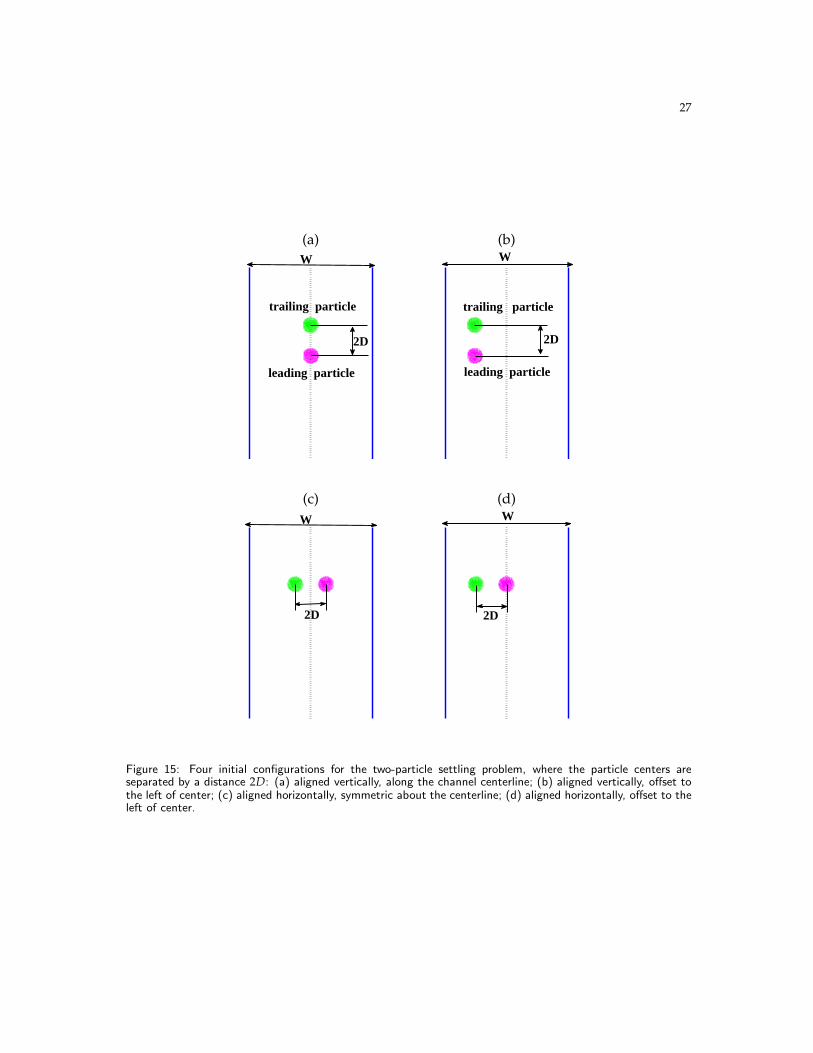
This section investigates the interactions between two circular particles with identicaldiameter D that are settling in a channel of length Ly = 3. We consider several initialconfigurations pictured in Figure 15, and again compare the solution at different valuesof Reynolds number by varying viscosity over the range µ∈ [0.0015,0.16].

We begin by describing a well-known phenomenon in particle suspension flows whereinpairs of particles interact and undergo a “drafting, kissing and tumbling” behavior (whichwe abbreviate by DKT). This phenomenon has been established experimentally in paperssuch as [18, 31] and demonstrated numerically in [17], and can be justified physically asfollows. The leading particle creates in its wake a reduction of pressure as it falls underthe influence of gravity. Provided that the trailing particle is close enough to interact withthis wake, it experiences a smaller drag force than the leading particle. As a result thetrailing particle falls faster and the particles approach each other – this is the initiation ofthe “drafting phase”. As the distance between the particles decreases, they eventually be-come close enough to nearly touch, which is referred to as “kissing”. The kissing particlesmomentarily form a single longer body that is aligned parallel with the flow; however,this parallel arrangement is unstable and the particles eventually tumble relative to eachother and swap leading/trailing positions – this is the “tumbling phase”. The particlessubsequently separate and one of two things happens: either the DKT process repeats,or the particles continue to separate until the interaction force becomes so weak that theyfall independently at their “natural” wall-corrected vertical settling velocity [42].

The simulations in this section are performed using the four initial configurations

27

(a) (b)

2D

W

trailing particle

leading particle

W

2D

trailing particle

leading particle

(c) (d)

W

2D

W

2D

Figure 15: Four initial configurations for the two-particle settling problem, where the particle centers areseparated by a distance 2D: (a) aligned vertically, along the channel centerline; (b) aligned vertically, offset tothe left of center; (c) aligned horizontally, symmetric about the centerline; (d) aligned horizontally, offset to theleft of center.

28

depicted in Figure 15:

(a) Aligned vertically, one above the other along the channel centerline.

(b) Aligned vertically, but shifted to the left to a position midway between the channelcenterline and the left wall.

(c) Aligned horizontally, and placed symmetrically about the centerline.

(d) Aligned horizontally, but shifted to the left of center.

In all cases, the particle diameter is D = 0.08 cm and the initial separation distance be-tween the centers of mass of the two particles is 2D. As in the previous section, we alsoconsider two channel widths, W=4D and W=8D.

5.1 Two vertically-aligned particles, released along the centerline

As a first test of the two-particle case, we use the initial set-up shown in Figure 15(a)wherein the particles are both released along the centerline with their centers of massseparated vertically by a distance 2D. We perform simulations with channel width W =8D and three different Reynolds numbers, Re=3, 14 and 80.

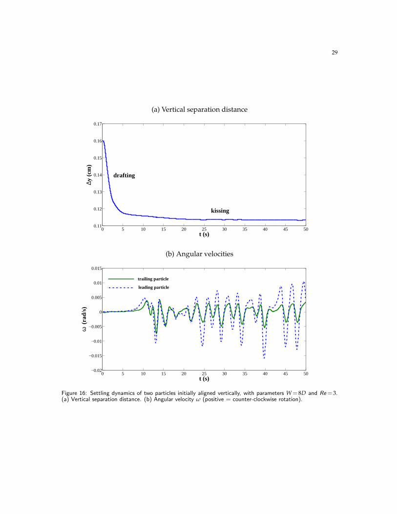
Starting with the smallest value of Re=3, we find that both particles remain along thechannel centerline throughout the simulation, and while drafting and kissing behavior isobserved, no tumbling occurs. As seen in Figure 16(a), the trailing particle approachesquite close to the leading particle, but never touches it. This is because of the increase inthe effective diameter of the particle owing to the delta function smoothing radius, as wasdiscussed already at the end of section 4.3.2. After kissing, the particles continue to fall asa single body with no significant relative motion, except for a very slight “wobble” thatcorresponds to a small-amplitude oscillation in the orientation angle (refer to the angularvelocity plot in Figure 16(b)). This motion can be attributed primarily to oscillations ofthe IB points making up the particles that arises from the IB spring forces driving slightdeviations from the equilibrium (stress-free) state; this is an artifact of the IB method thatis not present in actual solid particles.

Upon increasing the Reynolds number to Re= 14 the dynamics become much morecomplex. The trailing particle catches up with and subsequently passes the leading par-ticle at time t≈11 s, breaking the left-right symmetry. This tumbling behavior is evidentin Figure 17(a) where the vertical separation distance becomes negative. After the firsttumble, the particles separate horizontally and move to locations symmetrically oppositeeach other relative to the centerline and separated by a horizontal distance of roughly0.27 cm. They continue to fall vertically at approximately the same x locations, and forthe next 20 seconds they exchange leading and trailing positions via a small periodicvariation in the vertical velocity whose amplitude decreases in time. By time t ≈ 35 s,the particles have essentially reached a steady state in which they are falling at constantvelocity and maintaining a constant separation distance (refer to Figure 17(b)).

29

(a) Vertical separation distance

0 5 10 15 20 25 30 35 40 45 500.11

0.12

0.13

0.14

0.15

0.16

0.17

∆y (

cm)

t (s)

drafting

kissing

(b) Angular velocities

0 5 10 15 20 25 30 35 40 45 50−0.02

−0.015

−0.01

−0.005

0

0.005

0.01

0.015

t (s)

ω (

rad/

s)

trailing particle

leading particle

Figure 16: Settling dynamics of two particles initially aligned vertically, with parameters W = 8D and Re= 3.(a) Vertical separation distance. (b) Angular velocity ω (positive = counter-clockwise rotation).

30

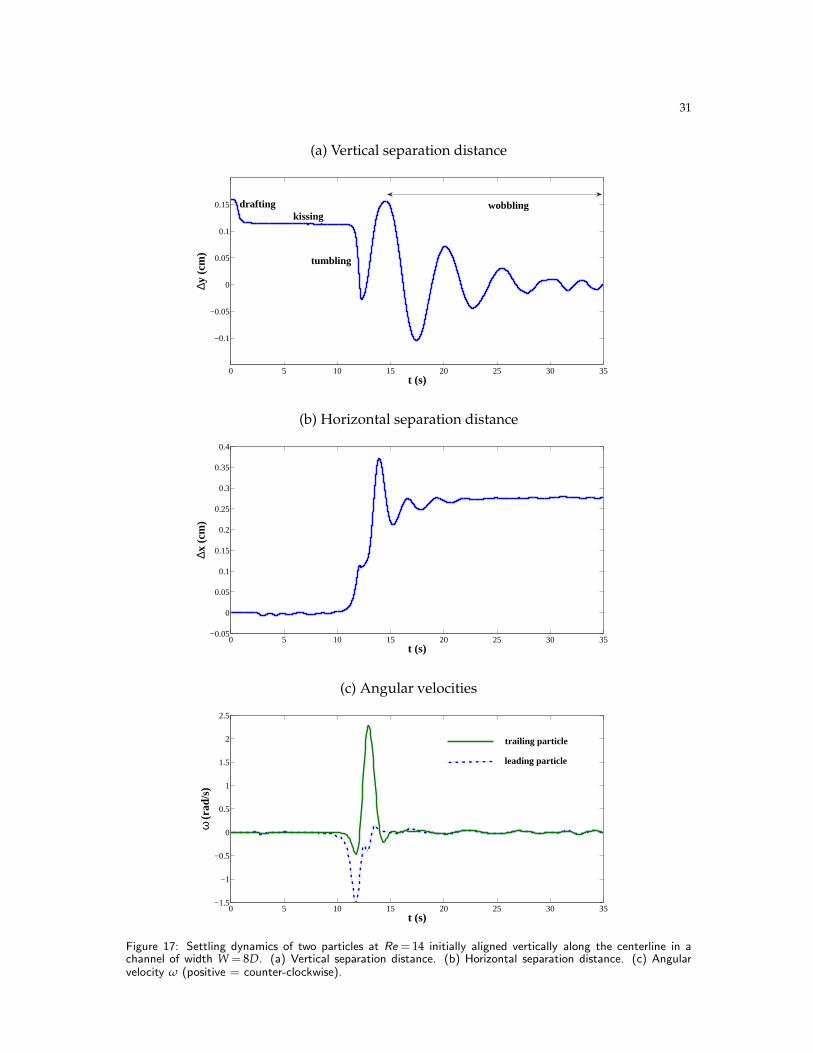
The angular velocity plot in Figure 17(c) shows that both particles experience a sig-nificant rotation during the tumbling phase that is several orders of magnitude largerthan the small “wobbling” motion observed in the Re=3 case. In fact, the growth of thisrotational motion appears to be connected with the breaking of the horizontal symmetrythat initiates the tumbling motion. By time t=15 s, the rotational motion has subsided.

Because of the symmetry in both the initial conditions and the governing equations,one would expect that the numerical solution should remain symmetric for all time, re-gardless of Reynolds number. The most likely source of asymmetry that initiates thetumbling behavior observed in the higher Re simulation is numerical error – these errorsare sufficiently damped out when Re=3, but remain large enough to initiate tumbling atRe=14. This conjecture is borne out by the simulations in section 5.2, where two particlesare aligned vertically and released off-center. We have nonetheless shown the results forthis symmetric initial condition since it is commonly studied in other simulations [17].

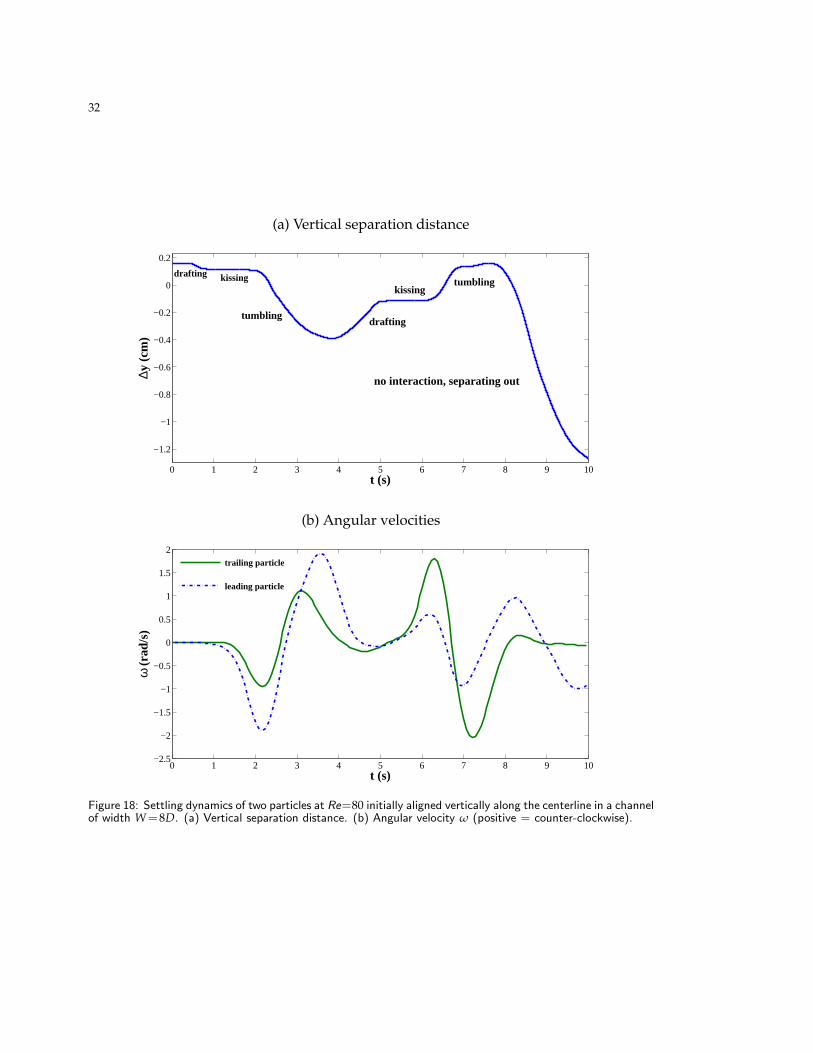
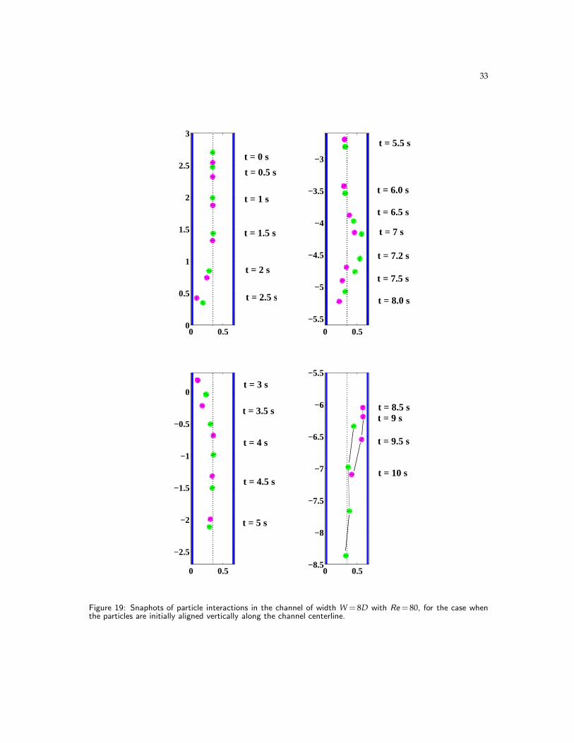
As the Reynolds number is increased yet further to Re= 80, we observe in Figure 18another qualitative change in solution behavior that is most easily seen in the sequenceof snapshots collected in Figure 19. The two particles begin with a DKT exchange such asthat observed for Re=14, however this occurs as the two particles drift together towardthe left channel wall (instead of toward the channel centerline). Following that, the par-ticles drift reverse direction toward the right wall and undergo a second DKT exchange,after which the particle that was initially trailing ends up in the lead. These two DKTexchanges are accompanied by a back-and-forth rotational motion of each particle thathas an amplitude similar in size to the Re= 14 case (refer to Figure 18(b)). Once again,it appears to be growth in the small “wobble” in the particle angular velocity plot thatinitiates tumbling. We also observe that when a particle nears the left wall it experiencesa clockwise rotation, while the direction of rotation is reversed near the right wall – this isconsistent with physical intuition, which suggests that wall drag arising from the no-slipcondition at the channel wall should cause a rolling-type motion as the portion of theparticle closest to the wall slows down.

FHJ [17] have performed a similar computation at Re= 70 (for the same symmetricinitial conditions) that exhibits results consistent with ours up to time t≈5.4 s. However,they terminate their computation at this point and there is no indication in their paperof the subsequent dynamics. We have computed beyond this time and find that after thesecond tumble, the particles separate vertically as they migrate toward the center of thechannel. By time t=10 s they settle at roughly the same speed and no longer interact inany significant way. Our computations also exhibit much the same qualitative behavioras the experiments reported in [18, 31] and numerical simulations from [20, 51].

5.2 Two vertically-aligned particles, released off-center

In this section, we consider an asymmetric initial layout where the two particles arealigned vertically (again separated by a distance 2D) but instead have their centers ofmass displaced to the left of center at location x=W/4. This initial geometry is depicted

31

(a) Vertical separation distance

0 5 10 15 20 25 30 35

−0.1

−0.05

0

0.05

0.1

0.15

t (s)

∆y (

cm)

drafting

tumbling

wobblingkissing

(b) Horizontal separation distance

0 5 10 15 20 25 30 35−0.05

0

0.05

0.1

0.15

0.2

0.25

0.3

0.35

0.4

t (s)

∆x (

cm)

(c) Angular velocities

0 5 10 15 20 25 30 35−1.5

−1

−0.5

0

0.5

1

1.5

2

2.5

t (s)

ω (

rad/

s)

trailing particle

leading particle

Figure 17: Settling dynamics of two particles at Re = 14 initially aligned vertically along the centerline in achannel of width W = 8D. (a) Vertical separation distance. (b) Horizontal separation distance. (c) Angularvelocity ω (positive = counter-clockwise).

32

(a) Vertical separation distance

0 1 2 3 4 5 6 7 8 9 10

−1.2

−1

−0.8

−0.6

−0.4

−0.2

0

0.2

t (s)

∆y (

cm)

drafting kissing

tumblingdrafting

kissing

no interaction, separating out

tumbling

(b) Angular velocities

0 1 2 3 4 5 6 7 8 9 10−2.5

−2

−1.5

−1

−0.5

0

0.5

1

1.5

2

t (s)

ω (

rad/

s)

trailing particle

leading particle

Figure 18: Settling dynamics of two particles at Re=80 initially aligned vertically along the centerline in a channelof width W=8D. (a) Vertical separation distance. (b) Angular velocity ω (positive = counter-clockwise).

33

0 0.50

0.5

1

1.5

2

2.5

3

t = 0.5 s

t = 0 s

t = 1.5 s

t = 1 s

t = 2 s

t = 2.5 s

0 0.5

−5.5

−5

−4.5

−4

−3.5

−3

t = 5.5 s

t = 7.5 s

t = 6.0 s

t = 6.5 s

t = 7 s

t = 7.2 s

t = 8.0 s

0 0.5

−2.5

−2

−1.5

−1

−0.5

0t = 3 s

t = 4 s

t = 5 s

t = 3.5 s

t = 4.5 s

0 0.5−8.5

−8

−7.5

−7

−6.5

−6

−5.5

t = 8.5 st = 9 s

t = 10 s

t = 9.5 s

Figure 19: Snaphots of particle interactions in the channel of width W = 8D with Re= 80, for the case whenthe particles are initially aligned vertically along the channel centerline.

34

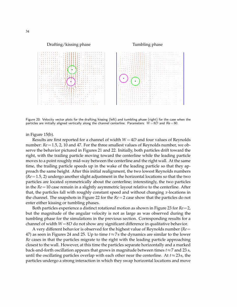
Drafting/kissing phase Tumbling phase

Figure 20: Velocity vector plots for the drafting/kissing (left) and tumbling phase (right) for the case when theparticles are initially aligned vertically along the channel centerline. Parameters: W=8D and Re=80.

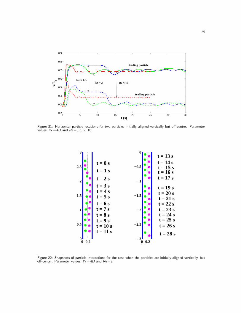
in Figure 15(b).Results are first reported for a channel of width W =4D and four values of Reynolds

number: Re=1.5, 2, 10 and 47. For the three smallest values of Reynolds number, we ob-serve the behavior pictured in Figures 21 and 22. Initially, both particles drift toward theright, with the trailing particle moving toward the centerline while the leading particlemoves to a point roughly mid-way between the centerline and the right wall. At the sametime, the trailing particle speeds up in the wake of the leading particle so that they ap-proach the same height. After this initial realignment, the two lowest Reynolds numbers(Re=1.5, 2) undergo another slight adjustment in the horizontal locations so that the twoparticles are located symmetrically about the centerline; interestingly, the two particlesin the Re=10 case remain in a slightly asymmetric layout relative to the centerline. Afterthat, the particles fall with roughly constant speed and without changing x-locations inthe channel. The snapshots in Figure 22 for the Re=2 case show that the particles do notenter either kissing or tumbling phases.

Both particles experience a distinct rotational motion as shown in Figure 23 for Re=2,but the magnitude of the angular velocity is not as large as was observed during thetumbling phase for the simulations in the previous section. Corresponding results for achannel of width W=8D do not show any significant difference in qualitative behavior.

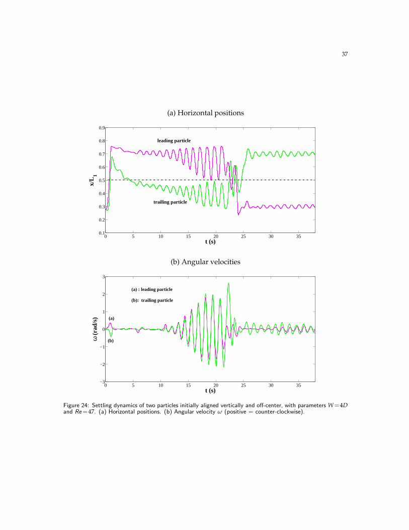
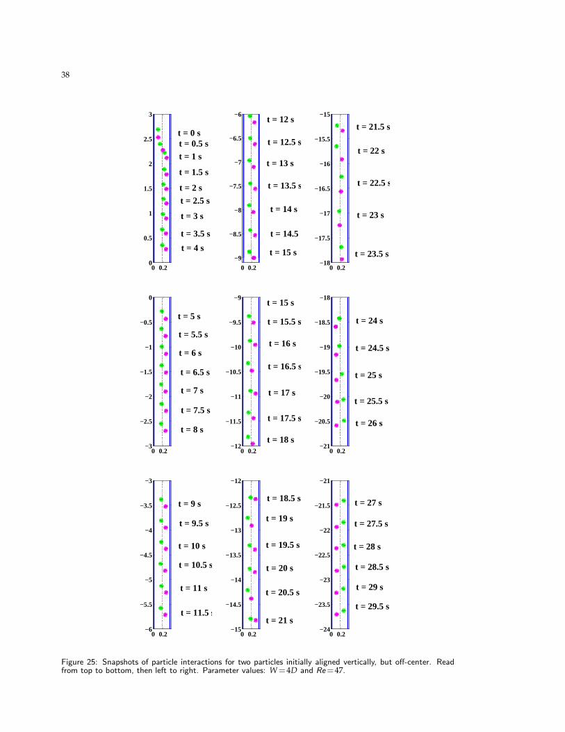
A very different behavior is observed for the highest value of Reynolds number (Re=47) as seen in Figures 24 and 25. Up to time t≈7 s the dynamics are similar to the lowerRe cases in that the particles migrate to the right with the leading particle approachingclosest to the wall. However, at this time the particles separate horizontally and a markedback-and-forth oscillation appears that grows in magnitude between times t≈7 and 23 s,until the oscillating particles overlap with each other near the centerline. At t≈23 s, theparticles undergo a strong interaction in which they swap horizontal locations and move

35

0 5 10 15 20 25 30 350.2

0.3

0.4

0.5

0.6

0.7

0.8

0.9

t (s)

x/L

1

trailing particle

leading particle

Re ≈ 1.5Re ≈ 2 Re ≈ 10

Figure 21: Horizontal particle locations for two particles initially aligned vertically but off-center. Parametervalues: W=4D and Re=1.5, 2, 10.

0 0.20

0.5

1

1.5

2

2.5

3

t = 11 s

t = 9 st = 8 st = 7 st = 6 st = 5 st = 4 st = 3 st = 2 s

t = 1 st = 0 s

t = 10 s

0 0.2−3

−2.5

−2

−1.5

−1

−0.5

0t = 13 st = 14 s

t = 28 s

t = 26 st = 25 st = 24 st = 23 st = 22 st = 21 st = 20 st = 19 s

t = 17 st = 16 st = 15 s

Figure 22: Snapshots of particle interactions for the case when the particles are initially aligned vertically, butoff-center. Parameter values: W=4D and Re=2.

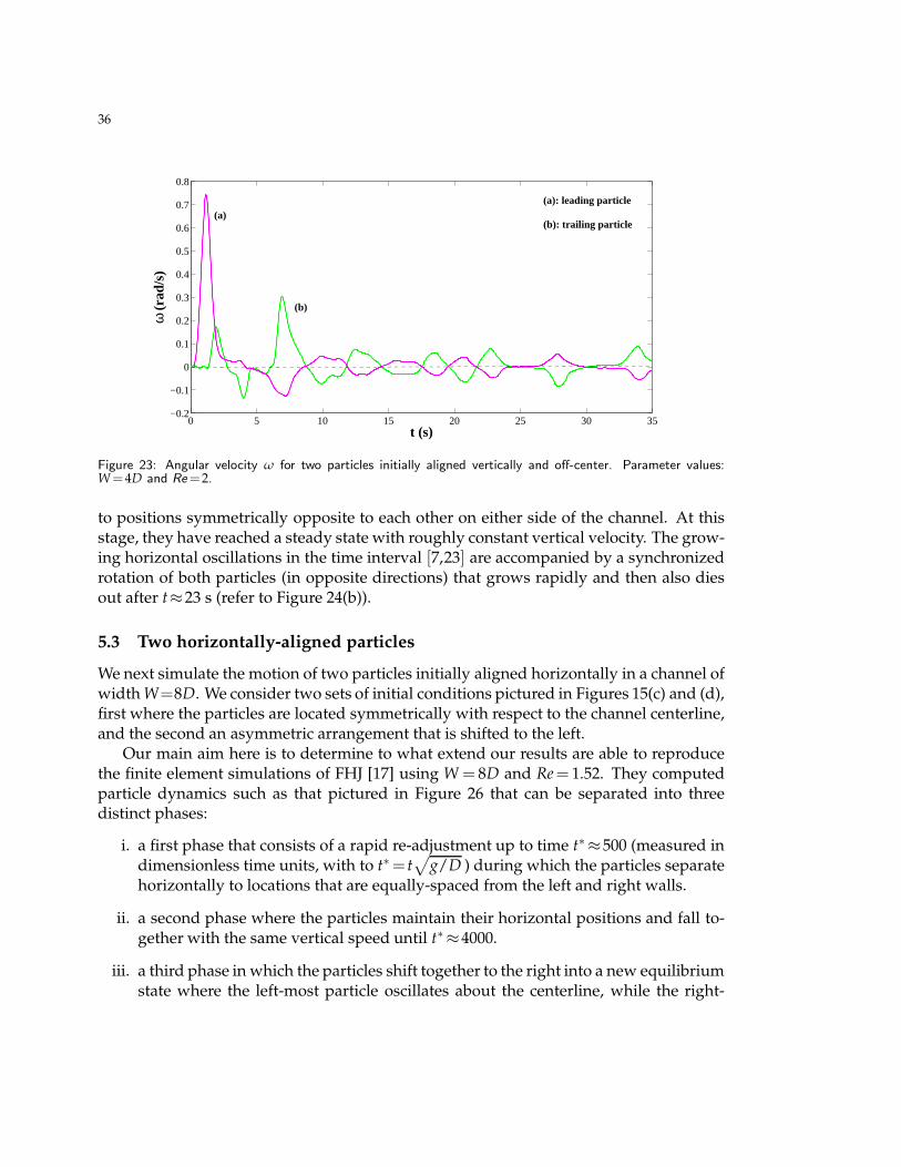
36

0 5 10 15 20 25 30 35−0.2

−0.1

0

0.1

0.2

0.3

0.4

0.5

0.6

0.7

0.8

t (s)

ω (

rad/

s)

(a): leading particle

(b): trailing particle(a)

(b)

Figure 23: Angular velocity ω for two particles initially aligned vertically and off-center. Parameter values:W=4D and Re=2.

to positions symmetrically opposite to each other on either side of the channel. At thisstage, they have reached a steady state with roughly constant vertical velocity. The grow-ing horizontal oscillations in the time interval [7,23] are accompanied by a synchronizedrotation of both particles (in opposite directions) that grows rapidly and then also diesout after t≈23 s (refer to Figure 24(b)).

5.3 Two horizontally-aligned particles

We next simulate the motion of two particles initially aligned horizontally in a channel ofwidth W=8D. We consider two sets of initial conditions pictured in Figures 15(c) and (d),first where the particles are located symmetrically with respect to the channel centerline,and the second an asymmetric arrangement that is shifted to the left.

Our main aim here is to determine to what extend our results are able to reproducethe finite element simulations of FHJ [17] using W = 8D and Re= 1.52. They computedparticle dynamics such as that pictured in Figure 26 that can be separated into threedistinct phases:

i. a first phase that consists of a rapid re-adjustment up to time t∗≈500 (measured indimensionless time units, with to t∗= t

√g/D ) during which the particles separate

horizontally to locations that are equally-spaced from the left and right walls.

ii. a second phase where the particles maintain their horizontal positions and fall to-gether with the same vertical speed until t∗≈4000.

iii. a third phase in which the particles shift together to the right into a new equilibriumstate where the left-most particle oscillates about the centerline, while the right-

37

(a) Horizontal positions

0 5 10 15 20 25 30 350.1

0.2

0.3

0.4

0.5

0.6

0.7

0.8

0.9

t (s)

x/L

1

leading particle

trailing particle

(b) Angular velocities

0 5 10 15 20 25 30 35−3

−2

−1

0

1

2

3

t (s)

ω (

rad/

s) (a)

(a) : leading particle

(b): trailing particle

(b)

Figure 24: Settling dynamics of two particles initially aligned vertically and off-center, with parameters W=4Dand Re=47. (a) Horizontal positions. (b) Angular velocity ω (positive = counter-clockwise).

38

0 0.20

0.5

1

1.5

2

2.5

3

t = 0 s

t = 4 s

t = 3.5 s

t = 2.5 st = 2 s

t = 1.5 s

t = 0.5 st = 1 s

t = 3 s

0 0.2−9

−8.5

−8

−7.5

−7

−6.5

−6t = 12 s

t = 14.5 s

t = 15 s

t = 14 s

t = 13.5 s

t = 13 s

t = 12.5 s

0 0.2−18

−17.5

−17

−16.5

−16

−15.5

−15

t = 23.5 s

t = 21.5 s

t = 22 s

t = 22.5 s

t = 23 s

0 0.2−3

−2.5

−2

−1.5

−1

−0.5

0

t = 5 s

t = 8 s

t = 7.5 s

t = 7 s

t = 6.5 s

t = 6 s

t = 5.5 s

0 0.2−12

−11.5

−11

−10.5

−10

−9.5

−9t = 15 s

t = 18 s

t = 17 s

t = 16.5 s

t = 16 s

t = 17.5 s

t = 15.5 s

0 0.2−21

−20.5

−20

−19.5

−19

−18.5

−18

t = 24 s

t = 24.5 s

t = 25 s

t = 25.5 s

t = 26 s

0 0.2−6

−5.5

−5

−4.5

−4

−3.5

−3

t = 11.5 s

t = 9 s

t = 9.5 s

t = 10 s

t = 10.5 s

t = 11 s

0 0.2−15

−14.5

−14

−13.5

−13

−12.5

−12

t = 18.5 s

t = 19 s

t = 19.5 s

t = 20 s

t = 20.5 s

t = 21 s

0 0.2−24

−23.5

−23

−22.5

−22

−21.5

−21

t = 29.5 s

t = 27 s

t = 27.5 s

t = 28 s

t = 28.5 s

t = 29 s

Figure 25: Snapshots of particle interactions for two particles initially aligned vertically, but off-center. Readfrom top to bottom, then left to right. Parameter values: W=4D and Re=47.

39

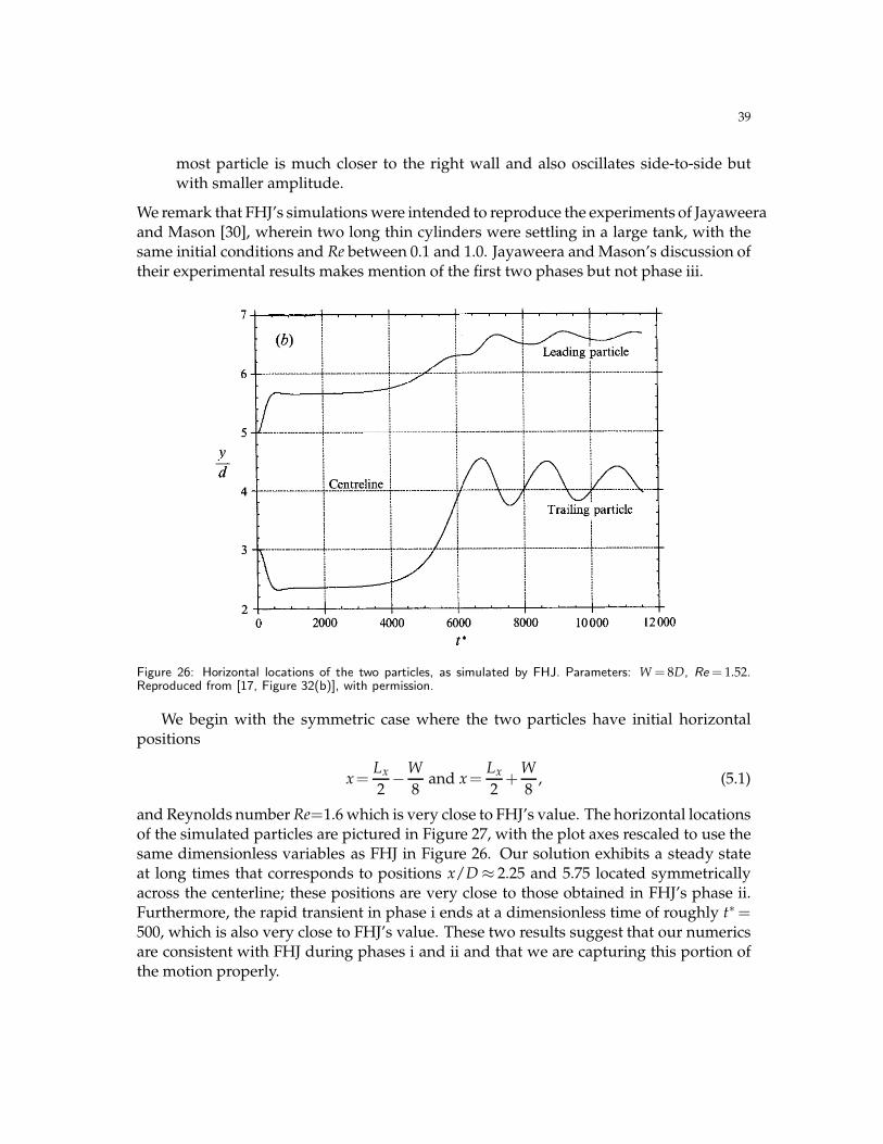
most particle is much closer to the right wall and also oscillates side-to-side butwith smaller amplitude.

We remark that FHJ’s simulations were intended to reproduce the experiments of Jayaweeraand Mason [30], wherein two long thin cylinders were settling in a large tank, with thesame initial conditions and Re between 0.1 and 1.0. Jayaweera and Mason’s discussion oftheir experimental results makes mention of the first two phases but not phase iii.

Figure 26: Horizontal locations of the two particles, as simulated by FHJ. Parameters: W = 8D, Re= 1.52.Reproduced from [17, Figure 32(b)], with permission.

We begin with the symmetric case where the two particles have initial horizontalpositions

x=Lx

2−W

8and x=

Lx

2+

W

8, (5.1)

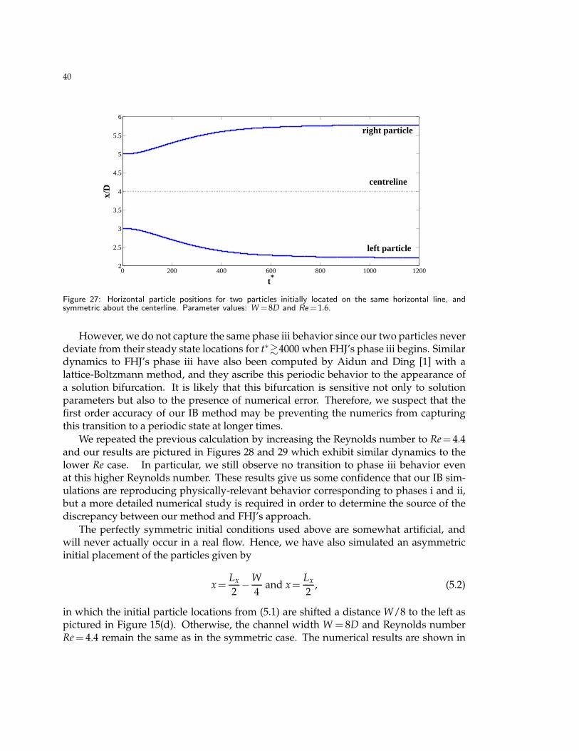
and Reynolds number Re=1.6 which is very close to FHJ’s value. The horizontal locationsof the simulated particles are pictured in Figure 27, with the plot axes rescaled to use thesame dimensionless variables as FHJ in Figure 26. Our solution exhibits a steady stateat long times that corresponds to positions x/D ≈ 2.25 and 5.75 located symmetricallyacross the centerline; these positions are very close to those obtained in FHJ’s phase ii.Furthermore, the rapid transient in phase i ends at a dimensionless time of roughly t∗=500, which is also very close to FHJ’s value. These two results suggest that our numericsare consistent with FHJ during phases i and ii and that we are capturing this portion ofthe motion properly.

40

0 200 400 600 800 1000 12002

2.5

3

3.5

4

4.5

5

5.5

6

t*

x/D

left particle

centreline

right particle

Figure 27: Horizontal particle positions for two particles initially located on the same horizontal line, andsymmetric about the centerline. Parameter values: W=8D and Re=1.6.

However, we do not capture the same phase iii behavior since our two particles neverdeviate from their steady state locations for t∗&4000 when FHJ’s phase iii begins. Similardynamics to FHJ’s phase iii have also been computed by Aidun and Ding [1] with alattice-Boltzmann method, and they ascribe this periodic behavior to the appearance ofa solution bifurcation. It is likely that this bifurcation is sensitive not only to solutionparameters but also to the presence of numerical error. Therefore, we suspect that thefirst order accuracy of our IB method may be preventing the numerics from capturingthis transition to a periodic state at longer times.

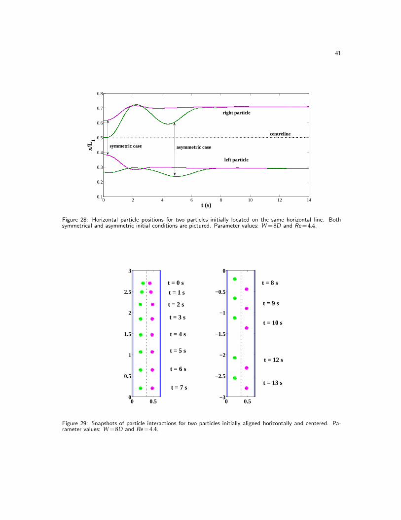
We repeated the previous calculation by increasing the Reynolds number to Re=4.4and our results are pictured in Figures 28 and 29 which exhibit similar dynamics to thelower Re case. In particular, we still observe no transition to phase iii behavior evenat this higher Reynolds number. These results give us some confidence that our IB sim-ulations are reproducing physically-relevant behavior corresponding to phases i and ii,but a more detailed numerical study is required in order to determine the source of thediscrepancy between our method and FHJ’s approach.

The perfectly symmetric initial conditions used above are somewhat artificial, andwill never actually occur in a real flow. Hence, we have also simulated an asymmetricinitial placement of the particles given by

x=Lx

2−W

4and x=

Lx

2, (5.2)

in which the initial particle locations from (5.1) are shifted a distance W/8 to the left aspictured in Figure 15(d). Otherwise, the channel width W = 8D and Reynolds numberRe= 4.4 remain the same as in the symmetric case. The numerical results are shown in

41

0 2 4 6 8 10 12 140.1

0.2

0.3

0.4

0.5

0.6

0.7

0.8

t (s)

x/L

1

right particle

left particle

asymmetric casesymmetric case

centreline

Figure 28: Horizontal particle positions for two particles initially located on the same horizontal line. Bothsymmetrical and asymmetric initial conditions are pictured. Parameter values: W=8D and Re=4.4.

0 0.50

0.5

1

1.5

2

2.5

3

t = 0 s

t = 1 s

t = 2 s

t = 3 s

t = 4 s

t = 5 s

t = 6 s

t = 7 s

0 0.5−3

−2.5

−2

−1.5

−1

−0.5

0

t = 8 s

t = 9 s

t = 12 s

t = 13 s

t = 10 s

Figure 29: Snapshots of particle interactions for two particles initially aligned horizontally and centered. Pa-rameter values: W=8D and Re=4.4.

42

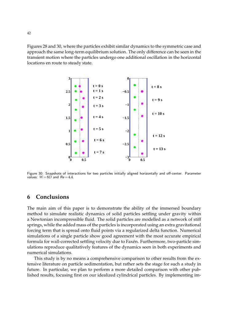
Figures 28 and 30, where the particles exhibit similar dynamics to the symmetric case andapproach the same long-term equilibrium solution. The only difference can be seen in thetransient motion where the particles undergo one additional oscillation in the horizontallocations en route to steady state.

0 0.50

0.5

1

1.5

2

2.5

3

t = 0 st = 1 s

t = 4 s

t = 7 s

t = 2 s

t = 3 s

t = 5 s

t = 6 s

0 0.5−3

−2.5

−2

−1.5

−1

−0.5

0

t = 8 s

t = 10 s

t = 9 s

t = 13 s

t = 12 s

Figure 30: Snapshots of interactions for two particles initially aligned horizontally and off-center. Parametervalues: W=8D and Re=4.4.

6 Conclusions

The main aim of this paper is to demonstrate the ability of the immersed boundarymethod to simulate realistic dynamics of solid particles settling under gravity withina Newtonian incompressible fluid. The solid particles are modelled as a network of stiffsprings, while the added mass of the particles is incorporated using an extra gravitationalforcing term that is spread onto fluid points via a regularized delta function. Numericalsimulations of a single particle show good agreement with the most accurate empiricalformula for wall-corrected settling velocity due to Faxen. Furthermore, two-particle sim-ulations reproduce qualitatively features of the dynamics seen in both experiments andnumerical simulations.

This study is by no means a comprehensive comparison to other results from the ex-tensive literature on particle sedimentation, but rather sets the stage for such a study infuture. In particular, we plan to perform a more detailed comparison with other pub-lished results, focusing first on our idealized cylindrical particles. By implementing im-

43

provements to the numerical algorithm that increase accuracy of the solution approxima-tion (such as in [34]) we hope to be able to explain the discrepancy we observed betweenour results and those of Feng, Hu and Joseph [17]. After that, the natural next step wouldbe to extend our numerical method to 3D in order to permit simulations spherical particleinteractions in a more realistic geometry.

We emphasize that this study is a “proof-of-concept” that the immersed boundarymethod may be applied to simulating the sedimentation of particles that are denser thanthe suspending fluid. We make no claim to improve on or to compete with other numer-ical methods that are specially-tailored to deal with rigid, non-deformable particles. In-stead, our ultimate goal is to solve sedimentation problems involving irregularly-shapedand highly deformable particles, which to our knowledge has not been sufficiently wellstudied in the literature. Such particle systems arise in the study of suspensions of redblood cells, wood pulp fibers, vesicles, bubbles, etc. Making use of the uniform triangu-lated meshes from the DistMesh package will allow us to deal with more general particleshapes. Furthermore, we plan to take advantage of recent developments in massivelyparallel immersed boundary algorithms by Wiens and Stockie [56], which should proveinstrumental in allowing efficient 2D and 3D immersed boundary simulations to be per-formed for non-dilute suspensions containing large numbers of particles.

Acknowledgments

This work was supported by grants from the Natural Sciences and Engineering ResearchCouncil of Canada and the Mprime Network of Centres of Excellence.

References

[1] C. K. Aidun and E.-J. Ding. Dynamics of particle sedimentation in a vertical channel: Period-doubling bifurcation and chaotic state. Phys. Fluids, 15(6):1612–1621, 2003.

[2] E. Alpkvist and I. Klapper. Description of mechanical response including detachment usinga novel particle model of biofilm/flow interaction. Water Sci. Tech., 55:265–273, 2007.

[3] G. K. Batchelor. An Introduction to Fluid Dynamics. Cambridge University Press, 1967.[4] A. Ben Richou, A. Ambari, M. Lebey, and J. K. Naciri. Drag force on a circular cylinder

midway between two parallel plates at Re ≪ 1. Part 2: moving uniformly (numerical andexperimental). Chem. Eng. Sci., 60(10):2535–2543, 2005.

[5] A. Ben Richou, A. Ambari, and J. K. Naciri. Drag force on a circular cylinder midway be-tween two parallel plates at Re ≪ 1. Part 1: Poiseuille flow (numerical). Chem. Eng. Sci.,59(15):3215–3222, 2004.

[6] D. Boffi, L. Gastaldi, and L. Heltai. On the CFL condition for the finite element immersedboundary method. Comput. Struct., 85:775–783, 2007.

[7] H. Brenner. Hydrodynamic resistance of particles at small Reynolds number. Adv. Chem.Eng., 6:287–438, 1966.

[8] W.-P. Breugem. A second-order accurate immersed boundary method for fully resolvedsimulations of particle-laden flows. J. Comput. Phys., 231(13):4469–4498, 2012.

44

[9] T. T. Bringley. Analysis of the Immersed Boundary Method for Stokes Flow. PhD thesis, Depart-ment of Mathematics, New York University, May 2008.

[10] R. Burger and W. L. Wendland. Sedimentation and suspension flows: Historical perspectiveand some recent developments. J. Eng. Math., 41:101–116, 2001.

[11] S. Champmartin and A. Ambari. Kinematics of a symmetrically confined cylindrical particlein a “Stokes-type” regime. Phys. Fluids, 19:073303, 2007.

[12] R. P. Chhabra, S. Agarwal, and K. Chaudhary. A note on wall effect on the terminal fallingvelocity of a sphere in quiescent Newtonian media in cylindrical tubes. Powder Tech., 129:53–58, 2003.

[13] R. H. Davis and A. Acrivos. Sedimentation of noncolloidal particles at low Reynolds num-bers. Annu. Rev. Fluid Mech., 17:91–118, 1985.

[14] R. Di Felice. The sedimentation velocity of dilute suspensions of nearly monosized spheres.Int. J. Multiphase Flow, 25:559–574, 1999.

[15] A. Dupuis, P. Chatelain, and P. Koumoutsakos. An immersed boundary-lattice-Boltzmannmethod for the simulation of the flow past an impulsively started cylinder. J. Comput. Phys.,227(9):4486–4498, 2008.

[16] O. H. Faxen. Forces exerted on a rigid cylinder in a viscous fluid between two parallel fixedplanes. Proceedings of the Royal Swedish Academy of Sciences, 187:1–13, 1946.

[17] J. Feng, H. H. Hu, and D. D. Joseph. Direct simulation of initial value problems for themotion of solid bodies in a Newtonian fluid. Part 1. Sedimentation. J. Fluid Mech., 261:95–134, 1994.

[18] A. F. Fortes, D. D. Joseph, and T. S. Lundgren. Nonlinear mechanics of fluidization of bedsof spherical particles. J. Fluid Mech., 177:467–483, 1987.

[19] S. Ghosh. The immersed boundary method for simulating gravitational settling and fluid shear-induced deformation of elastic structures. PhD thesis, Department of Mathematics, Simon FraserUniversity, Burnaby, Canada, Mar. 2013.

[20] R. Glowinski, T. W. Pan, T. I. Hesla, D. D. Joseph, and J. Periaux. A fictitious domain ap-proach to the direct numerical simulation of incompressible viscous flow past moving rigidbodies: Application to particulate flow. J. Comput. Phys., 169(2):363–426, 2001.

[21] B. E. Griffith, R. D. Hornung, D. M. McQueen, and C. S. Peskin. An adaptive, formally sec-ond order accurate version of the immersed boundary method. J. Comput. Phys., 223(1):10–49, 2007.

[22] E. Guazzelli and J. F. Morris. A Physical Introduction to Suspension Dynamics. CambridgeTexts in Applied Mathematics. Cambridge University Press, 2012.

[23] S. Haeri and J. S. Shrimpton. On the application of immersed boundary, fictitious domainand body-conformal mesh methods to many particle multiphase flows. Int. J. MultiphaseFlow, 40:38–55, 2012.

[24] J. Happel and H. Brenner. Low Reynolds number hydrodynamics, with special applications toparticulate media. Mechanics of fluids and transport processes. Martinus Nijhoff Publishers,1983.

[25] J. P. Hernandez-Ortiz. Boundary Integral Equations for Viscous Flows – non-Newtonian Behaviorand Solid Inclusions. PhD thesis, University of Wisconsin-Madison, Department of Mechani-cal Engineering, 2004.

[26] M. M. Hopkins and L. J. Fauci. A computational model of the collective fluid dynamics ofmotile microorganisms. J. Fluid Mech., 455:149–174, 2002.

[27] T. Y. Hou and Z. Shi. Removing the stiffness of elastic force from the immersed boundarymethod for the 2D Stokes equations. J. Comput. Phys., 227:9138–9169, 2008.

45

[28] H. H. Hu. Direct simulation of flows of solid-liquid mixtures. Int. J. Multiphase Flow,22(2):335–352, 1996.

[29] H. H. Hu, D. D. Joseph, and A. F. Fortes. Experiments and direct simulation of fluid particlemotions. Int. Vid. J. Eng. Res., 2:17–24, 1997.

[30] K. O. L. F. Jayaweera and B. J. Mason. The behaviour of freely falling cylinders and cones ina viscous fluid. J. Fluid Mech., 22(4):709–720, 1965.

[31] D. D. Joseph, A. Fortes, T. S. Lundgren, and P. Singh. Nonlinear mechanics of fluidizationof spheres, cylinders and disks in water. In Advances in Multiphase Flow and Related Problems,pages 101–122. SIAM, Philadelphia, PA, 1987.

[32] A. J. C. Ladd. Numerical simulations of particulate suspensions via a discretized Boltzmannequation. Part II. Numerical results. J. Fluid Mech., 271:311–339, 1994.

[33] M.-C. Lai. Simulations of the flow past an array of circular cylinders as a test of the immersedboundary method. PhD thesis, New York University, Sept. 1998.

[34] M.-C. Lai and C. S. Peskin. An immersed boundary method with formal second-order accu-racy and reduced numerical viscosity. J. Comput. Phys., 160(2):705–719, 2000.

[35] R. Mittal and G. Iaccarino. Immersed boundary methods. Annu. Rev. Fluid Mech., 37:239–261,2005.

[36] R. Munster, O. Mierka, and S. Turek. Finite element-fictitious boundary methods (FEM-FBM) for 3D particulate flow. Int. J. Numer. Meth. Fluids, 69(2):294–313, 2012.

[37] P. O. Persson and G. Strang. A simple mesh generator in MATLAB. SIAM Review, 46(2):329–345, 2004.

[38] C. S. Peskin. The immersed boundary method. Acta Numer., 11:1–39, 2002.[39] N. Phan-Thien and X.-J. Fan. Viscoelastic mobility problem using a boundary element

method. J. Non-Newton. Fluid Mech., 105(2-3):131–152, 2002.[40] G. Pianet and E. Arquis. Simulation of particles in fluid: a two-dimensional benchmark for

a cylinder settling in a wall-bounded box. Euro. J. Mech. B Fluids, 27:309–321, 2008.[41] W. H. Press, S. A. Teukolsky, W. T. Vetterling, and B. P. Flannery. Numerical Recipes in C: The

Art of Scientific Computing. Cambridge University Press, second edition, 1992.[42] A. Prosperetti and G. Tryggvason, editors. Computational Methods for Multiphase Flow. Cam-

bridge University Press, 2007.[43] D. Qi. Lattice-Boltzmann simulations of particles in non-zero-Reynolds-number flows. J.

Fluid Mech., 385:41–62, 1999.[44] J. F. Richardson and W. N. Zaki. Sedimentation and fluidisation: Part I. Trans. Inst. Chem.

Eng., 32:35–53, 1954.[45] J. M. Stockie. Analysis and Computation of Immersed Boundaries, with Application to Pulp Fibres.

PhD thesis, Institute of Applied Mathematics, University of British Columbia, Vancouver,Canada, 1997. Available at http://circle.ubc.ca/handle/2429/7346.

[46] J. M. Stockie. Modelling and simulation of porous immersed boundaries. Comput. Struct.,87(11-12):701–709, 2009.

[47] G. G. Stokes. Section IV. Determination of the motion of a fluid about a sphere which movesuniformly with a small velocity. In Mathematical and Physical Papers, volume III of The Sourcesof Science, No. 33, pages 55–67. Cambridge University Press, Teddington, UK, second edition,1966. First published in 1901.

[48] D. Sucker and H. Brauer. Fluiddynamik bei quer angestromten Zylindern. Heat Mass Trans-fer, 8(3):149–158, 1975.

[49] Y. Takaisi. The drag on a circular cylinder moving with low speeds in a viscous liquidbetween two parallel walls. J. Phys. Soc. Japan, 10:685–693, 1955.

46

[50] C. Tu and C. S. Peskin. Stability and instability in the computation of flows with moving im-mersed boundaries: A comparison of three methods. SIAM J. Sci. Stat. Comput., 13(6):1361–1376, 1992.

[51] M. Uhlmann. An immersed boundary method with direct forcing for the simulation ofparticulate flows. J. Comput. Phys., 209:448–476, 2005.

[52] P. Vasseur and R. G. Cox. The lateral migration of spherical particles sedimenting in a stag-nant bounded fluid. J. Fluid Mech., 80(3):561–591, 1977.

[53] J. Wang and A. Layton. Numerical simulations of fiber sedimentation in Navier-Stokes flow.Commun. Comput. Phys., 5(1):61–83, 2009.

[54] Z. Wang, J. Fan, and K. Luo. Combined multi-direct forcing and immersed boundarymethod for simulating flows with moving particles. Int. J. Multiphase Flow, 34:283–302, 2008.

[55] C. M. White. The drag of cylinders in fluids at slow speeds. Proc. Roy. Soc. A, 186:472–479,1946.

[56] J. K. Wiens and J. M. Stockie. An efficient parallel immersed boundary algorithm using apseudo-compressible fluid solver. J. Comput. Phys., May 2013. Submitted, arXiv:1305.3976.

[57] L. Zhu and C. S. Peskin. Simulation of a flapping flexible filament in a flowing soap film bythe immersed boundary method. J. Comput. Phys., 179(2):452–468, 2002.