Investigation of granular batch sedimentation via DEM–CFD coupling

Granular Matter (2014) 16:921–932DOI 10.1007/s10035-014-0534-0

ORIGINAL PAPER

Investigation of granular batch sedimentation via DEM–CFDcoupling

T. Zhao · G. T. Houlsby · S. Utili

Received: 3 February 2014 / Published online: 12 November 2014© Springer-Verlag Berlin Heidelberg 2014

Abstract This paper presents three dimensional numeri-cal investigations of batch sedimentation of spherical parti-cles in water, by analyses performed by the discrete elementmethod (DEM) coupled with computational fluid dynam-ics (CFD). By employing this model, the features of bothmechanical and hydraulic behaviour of the fluid-solid mix-ture system are captured. Firstly, the DEM–CFD model isvalidated by the simulation of the sedimentation of a singlespherical particle, for which an analytical solution is avail-able. The numerical model can replicate accurately the set-tling behaviour of particles as long as the mesh size ratio(Dmesh/d) and model size ratio (W/Dmesh) are both largerthan a given threshold. During granular batch sedimentation,segregation of particles is observed at different locations inthe model. Coarse grains continuously accumulate at the bot-tom, leaving the finer grains deposited in the upper part of thegranular assembly. During this process, the excess pore waterpressure initially increases rapidly to a peak value, and thendissipates gradually to zero. Meanwhile, the compressibilityof the sediments decreases slowly as a soil layer builds upat the bottom. Consolidation of the deposited layer is causedby the self-weight of grains, while the compressibility of thesample decreases progressively.

Electronic supplementary material The online version of thisarticle (doi:10.1007/s10035-014-0534-0) contains supplementarymaterial, which is available to authorized users.

T. Zhao (B) · G. T. HoulsbyDepartment of Engineering Science, University of Oxford,Oxford OX1 3PJ, UKe-mail: [email protected]

S. UtiliSchool of Engineering, University of Warwick,Coventry CV4 7AL, UK

Keywords Granular batch sedimentation · DEM–CFDcoupling · Segregation · Pore water pressure · Effectivestress · Compressibility

1 Introduction

The sedimentation and consolidation processes of granu-lar materials are common in both terrestrial and submergedenvironments. In the natural environment, granular mate-rials often settle continuously towards the seabed, lake orriver floor to form a loose sediment layer. As the skeletonof the sediment layer is extremely compressible, it under-goes relatively large strain under additional loads. Sedimen-tation processes are very important for solid-liquid sepa-ration, as can be found in the fields of chemical, mining,wastewater, food, pharmaceutical and other industries [1–3]. The related research includes theoretical, experimentaland numerical investigations on a variety of materials [3–10].

During granular sedimentation, the average settling veloc-ity of a suspension is the most notable parameter quantifyingthe dynamic behaviour of the fluid-solid mixture system [11–15]. As first proposed by Kynch [4], the average settlingvelocity of a suspension depends only on the local concen-tration of solid materials (in addition to the characteristics ofthe particles and fluid). This statement has been validated byexperimental measurements of the grain settling rates in gran-ular suspension systems [6,8,16]. Numerical simulations ofsedimentation mainly focus on the settling and depositionalbehaviour of particles in either monodisperse [7,12,17] orpolydisperse [10,18] systems. This research reveals threedistinct zones in a grain settling system, enumerated fromtop to bottom as: 1. the hindered settling zone, where thesurface settling velocity is approximately constant; 2. the

123

http://dx.doi.org/10.1007/s10035-014-0534-0

922 T. Zhao et al.

transition zone where the settling rate decreases graduallytowards zero; and 3. the compression zone where a soil layeris formed at the bottom and consolidation occurs due to theself-weight of sediments. However, as reported by Richard-son and Zaki [7], zone 1 is absent for very fine flocculatedpulps, and the settling rate decreases progressively.

For many years, analytical and numerical investiga-tions of sedimentation employing empirical correlationsof the mixture properties based on laboratory experimentshave been reported [3,7,19–22]. However, a fully system-atic study of sedimentation is still lacking as the fluid-solid mixture presents a highly heterogeneous structurefeaturing a spatially non-uniform distribution of parti-cles [6,23]. The numerical investigation reported here isbased on the concept that the motion of particles is com-pletely governed by the Newtonian equations of motion,and interparticle collisions are modelled by the soft parti-cle approach [3]. The fluid flow is calculated by the Navier–Stokes equations [3,11,24]. Consequently, the discrete ele-ment method (DEM) [25] and computational fluid dynamics(CFD) [26] techniques can be used to study the mechanicaland hydraulic behaviour of particles and fluid flow, respec-tively. By coupling these two methods, a complete analysisof the sedimentation of a fluid-solid mixture system can beachieved [27].

The work presented here is part of a research effort toextend the DEM modelling of landslides [28–30] to the sub-merged case. The paper is organised as follows. We explainthe theory and methodology of the DEM and CFD in Sect. 2.The numerical investigation of granular sedimentation is pre-sented in Sect. 3. We first validate the DEM–CFD couplingmodel by simulating the sedimentation of a single sphericalparticle (Sect. 3.1). Then, we analyse the batch sedimen-tation of particles, examining the segregation of particles,generation and dissipation of excess pore water pressures,and evolution of contact force chains (Sect. 3.2). Section 4summarizes the results and main conclusions achieved by thework.

2 Theory and methodology

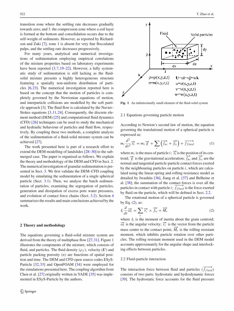
The equations governing a fluid-solid mixture system arederived from the theory of multiphase flow [27,31]. Figure 1illustrates the components of the mixture, which consists offluid, and particles. The fluid density (ρ f ), velocity (U) andparticle packing porosity (n) are functions of spatial posi-tion and time. The DEM and CFD open source codes ESyS-Particle [32,33] and OpenFOAM [34] were employed forthe simulations presented here. The coupling algorithm fromChen et al. [27] originally written in YADE [35] was imple-mented in ESyS-Particle by the authors.

Fig. 1 An infinitesimally small element of the fluid-solid system

2.1 Equations governing particle motion

According to Newton’s second law of motion, the equationgoverning the translational motion of a spherical particle isexpressed as:

mid2

dt2−→xi = mi

−→g +∑

c

(−→fnc + −→

ftc

)+ −−−→

f f luid (1)

where mi is the mass of particle i;−→xi is the position of its cen-troid; −→g is the gravitational acceleration;

−→fnc and

−→ftc are the

normal and tangential particle-particle contact forces exertedby the neighbouring particles on particle i , which are calcu-lated using the linear-spring and rolling resistance model asdetailed by Iwashita [36], Jiang et al. [37] and Belheine etal. [38]; the summation of the contact forces is over all theparticles in contact with particle i;−−−→

f f luid is the force exertedby fluid on the particle, which will be defined in Sect. 2.2.

The rotational motion of a spherical particle is governedby Eq. (2), as:

Iid

dt−→ωi =

∑

c

−→rc × −→ftc + −→

Mr (2)

where Ii is the moment of inertia about the grain centroid;−→ωi is the angular velocity; −→rc is the vector from the particlemass centre to the contact point;

−→Mr is the rolling resistant

moment, which inhibits particle rotation over other parti-cles. The rolling resistant moment used in the DEM modelaccounts approximately for the angular shape and interlock-ing effects between particles.

2.2 Fluid-particle interaction

The interaction force between fluid and particles (−−−→f f luid)

consists of two parts: hydrostatic and hydrodynamic forces[39]. The hydrostatic force accounts for the fluid pressure

123

Investigation of granular batch sedimentation 923

gradient around an individual particle (i.e. buoyancy) [27,40,41], expressed as:

−→f ib = −vpi∇ p (3)

where−→f ib is the hydrostatic buoyant force acting on particle

i, vpi is the volume of particle i; p is the fluid pressure.The hydrodynamic forces acting on a particle are the drag,

lift and virtual mass forces. The drag force is caused by theviscous shearing effect of fluid on the particle; the lift force iscaused by the high fluid velocity gradient-induced pressuredifference on the surface of the particle and the virtual massforce is caused by relative acceleration between particle andfluid [42–44]. The latter two forces are normally very smallwhen compared to the drag force in simulating fluid flow atrelatively low Reynolds numbers [44]. Therefore, the lift andvirtual mass forces are neglected in the current DEM–CFDcoupling model. In this process, the drag force occurs whenthere is a non-zero relative velocity between fluid and parti-cles. It acts at the particle centre in a direction opposite to theparticle motion relative to the fluid [45]. Experimental corre-lations [20,21,46] and numerical simulations [47–49] for thedrag force are reported in the literature. In this research, thedrag force (Fdi ) acting on an individual particle is calculatedusing the empirical correlation proposed by Di Felice [22],as:

Fdi = 1

2Cdρ f

πd2

4|U − V| (U − V) n−χ+1 (4)

where Cd is the drag force coefficient; d and V are particlediameter and velocity, respectively.

The porosity correction function n−(χ+1) in Eq. (4) rep-resents the influence of the packing concentration of grainson the drag force. The expression for the term χ is [22]:

χ = 3.7 − 0.65 exp

[−

(1.5 − log10 Rep

)2

2

](5)

where Rep = ρ f dn |U − V |/μ is the Reynolds numberdefined at the particle size level, with μ being the fluid vis-cosity. In the current analyses, χ ranges from 3.4 to 3.7.

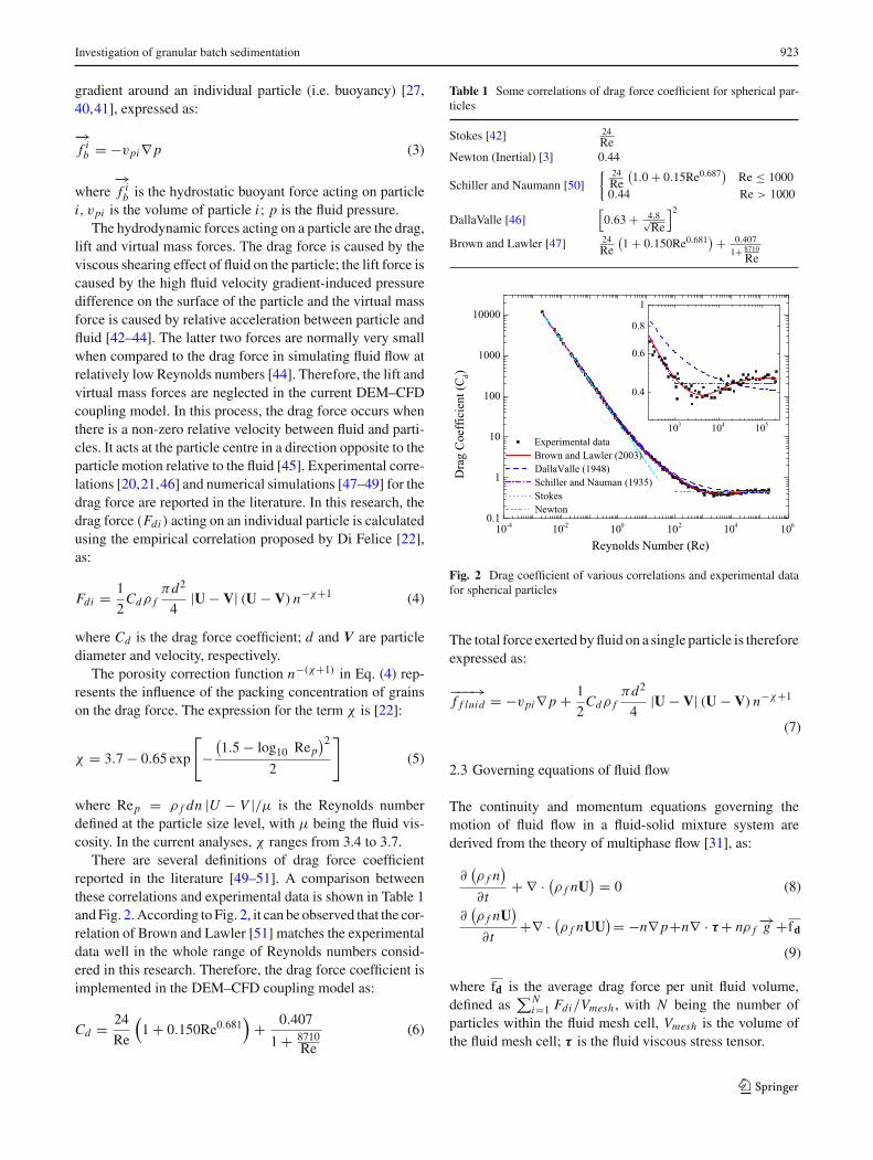
There are several definitions of drag force coefficientreported in the literature [49–51]. A comparison betweenthese correlations and experimental data is shown in Table 1and Fig. 2. According to Fig. 2, it can be observed that the cor-relation of Brown and Lawler [51] matches the experimentaldata well in the whole range of Reynolds numbers consid-ered in this research. Therefore, the drag force coefficient isimplemented in the DEM–CFD coupling model as:

Cd = 24

Re

(1 + 0.150Re0.681

)+ 0.407

1 + 8710Re

(6)

Table 1 Some correlations of drag force coefficient for spherical par-ticles

Stokes [42] 24Re

Newton (Inertial) [3] 0.44

Schiller and Naumann [50]

{ 24Re

(1.0 + 0.15Re0.687

)Re ≤ 1000

0.44 Re > 1000

DallaValle [46][0.63 + 4.8√

Re

]2

Brown and Lawler [47] 24Re

(1 + 0.150Re0.681

) + 0.4071+ 8710

Re

10-4 10-2 100 102 104 1060.1

1

10

100

1000

10000

Experimental data Brown and Lawler (2003)DallaValle (1948)Schiller and Nauman (1935)StokesNewton

Dra

g C

oeff

icie

nt (C

d)

Reynolds Number (Re)

103 104 105

0.4

0.6

0.8

1

Fig. 2 Drag coefficient of various correlations and experimental datafor spherical particles

The total force exerted by fluid on a single particle is thereforeexpressed as:

−−−→f f luid = −vpi∇ p + 1

2Cdρ f

πd2

4|U − V| (U − V) n−χ+1

(7)

2.3 Governing equations of fluid flow

The continuity and momentum equations governing themotion of fluid flow in a fluid-solid mixture system arederived from the theory of multiphase flow [31], as:

∂(ρ f n

)

∂t+ ∇ · (ρ f nU

) = 0 (8)

∂(ρ f nU

)

∂t+∇ · (

ρ f nUU)= −n∇ p+n∇ · τ + nρ f

−→g +fd

(9)

where fd is the average drag force per unit fluid volume,defined as

∑Ni=1 Fdi/Vmesh , with N being the number of

particles within the fluid mesh cell, Vmesh is the volume ofthe fluid mesh cell; τ is the fluid viscous stress tensor.

123

924 T. Zhao et al.

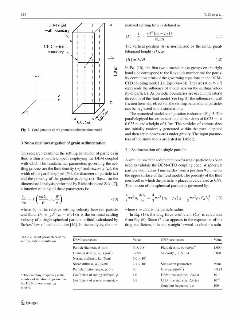
Fig. 3 Configuration of the granular sedimentation model

3 Numerical investigation of grain sedimentation

This research examines the settling behaviour of particles influid within a parallelepiped, employing the DEM coupledwith CFD. The fundamental parameters governing the set-tling process are the fluid density (ρ f ) and viscosity (μ), thewidth of the parallelepiped (W ), the diameter of particle (d)

and the porosity of the granular packing (n). Based on thedimensional analysis performed by Richardson and Zaki [7],a function relating all these parameters is:

Ur

U0= f

(ρdUr

µ, n,

W

d

)(10)

where Ur is the relative settling velocity between particleand fluid, U0 = gd2 (ρs − ρ)/18μ is the terminal settlingvelocity of a single spherical particle in fluid, calculated byStokes’ law of sedimentation [46]. In the analysis, the nor-

malized settling time is defined as:

[T ] = t

tc= gd2

(ρs − ρ f

)t

18μH(11)

The vertical position (h) is normalized by the initial paral-lelepiped height (H), as:

[H ] = h/H (12)

In Eq. (10), the first two dimensionless groups on the righthand side correspond to the Reynolds number and the poros-ity correction terms of the governing equations in the DEM–CFD coupling model (i.e. Eqs. (4)–(6)). The size ratio (W/d)

represents the influence of model size on the settling veloc-ity of particles. As periodic boundaries are used in the lateraldirections of the fluid model (see Fig. 3), the influence of wallfriction (non-slip effect) on the settling behaviour of particlescan be neglected in the simulations.

The numerical model configuration is shown in Fig. 3. Theparallelepiped has cross-sectional dimensions of 0.025 m ×0.025 m and a height of 1.0 m. The particles of various sizesare initially randomly generated within the parallelepipedand then settle downwards under gravity. The input parame-ters of the simulations are listed in Table 2.

3.1 Sedimentation of a single particle

A simulation of the sedimentation of a single particle has beenused to validate the DEM–CFD coupling code. A sphericalparticle with radius 1 mm settles from a position 9 cm belowthe upper surface of the fluid model. The porosity of the fluidmesh cell in which the particle is placed is calculated as 0.99.The motion of the spherical particle is governed by:

4

3πr3ρs

∂Ur

∂t= 4

3πr3 (

ρs − ρ f)

g − 1

2πr2ρ f CdU 2

r (13)

where r = d/2 is the particle radius.In Eq. (13), the drag force coefficient (Cd) is calculated

from Eq. (6). Since U also appears in the expression of thedrag coefficient, it is not straightforward to obtain a solu-

Table 2 Input parameters of thesedimentation simulation

∗ The coupling frequency is thenumber of iteration steps used inthe DEM in one couplinginterval

DEM parameters Value CFD parameters Value

Particle diameter, d (mm) [1.8, 3.8] Fluid density, ρ f (kg/m3) 1,000

Granular density, ρs (kg/m3) 2,650 Viscosity, μ (Pa · s) 0.001

Normal stiffness, Kn (N/m) 3.0 × 107

Shear stiffness, Ks (N/m) 2.7 × 107 Simulation parameters Value

Particle friction angle, φμ(◦) 30 Gravity, g(m/s2) −9.81

Coefficient of rolling stiffness, β 1.0 DEM time step size, ts(s) 10−7

Coefficient of plastic moment, η 0.1 CFD time step size, t f (s) 10−5

Coupling frequency∗, α 100

123


0.0 0.1 0.2 0.3 0.40.00

0.05

0.10

0.15

0.20

0.25

0.30

Settl

ing

velo

city

(m/s

)

Time (s)

Analytical results Numerical results

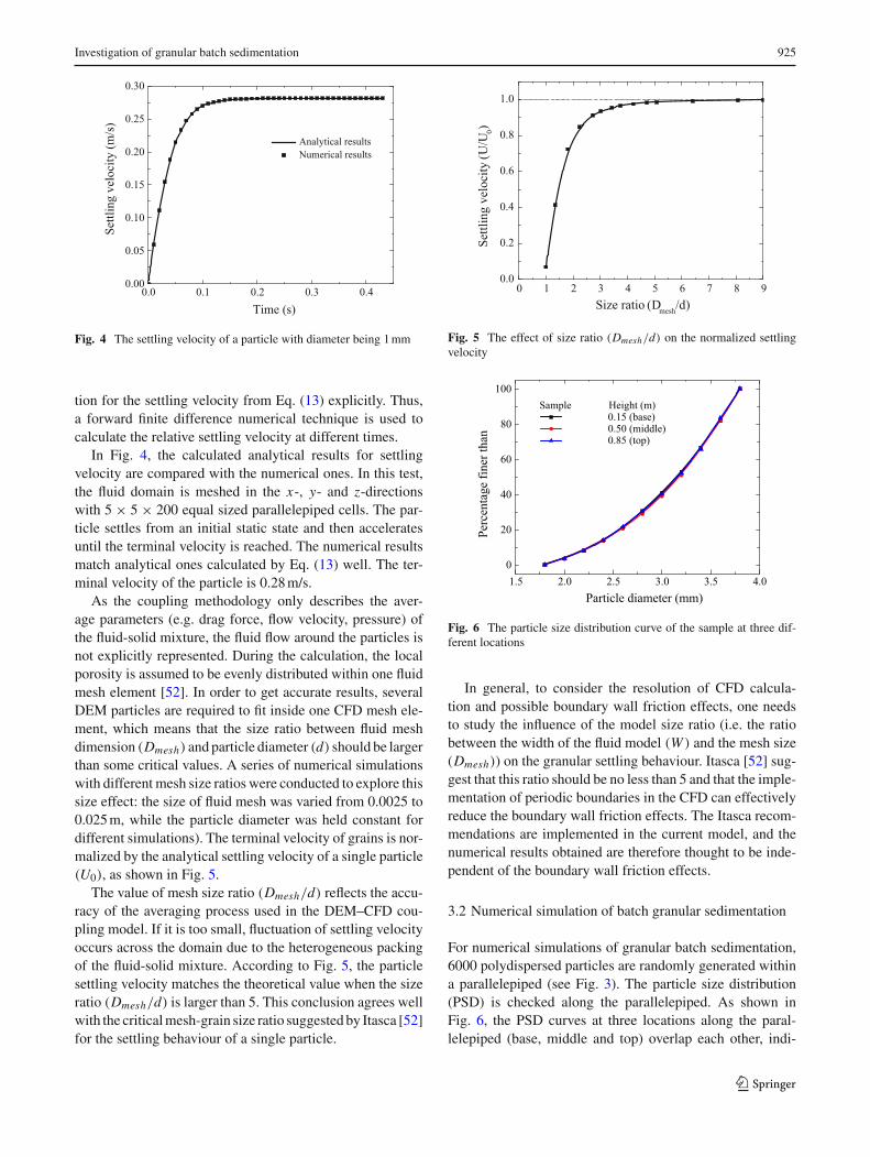
Fig. 4 The settling velocity of a particle with diameter being 1 mm

tion for the settling velocity from Eq. (13) explicitly. Thus,a forward finite difference numerical technique is used tocalculate the relative settling velocity at different times.

In Fig. 4, the calculated analytical results for settlingvelocity are compared with the numerical ones. In this test,the fluid domain is meshed in the x-, y- and z-directionswith 5 × 5 × 200 equal sized parallelepiped cells. The par-ticle settles from an initial static state and then acceleratesuntil the terminal velocity is reached. The numerical resultsmatch analytical ones calculated by Eq. (13) well. The ter-minal velocity of the particle is 0.28 m/s.

As the coupling methodology only describes the aver-age parameters (e.g. drag force, flow velocity, pressure) ofthe fluid-solid mixture, the fluid flow around the particles isnot explicitly represented. During the calculation, the localporosity is assumed to be evenly distributed within one fluidmesh element [52]. In order to get accurate results, severalDEM particles are required to fit inside one CFD mesh ele-ment, which means that the size ratio between fluid meshdimension (Dmesh) and particle diameter (d) should be largerthan some critical values. A series of numerical simulationswith different mesh size ratios were conducted to explore thissize effect: the size of fluid mesh was varied from 0.0025 to0.025 m, while the particle diameter was held constant fordifferent simulations). The terminal velocity of grains is nor-malized by the analytical settling velocity of a single particle(U0), as shown in Fig. 5.

The value of mesh size ratio (Dmesh/d) reflects the accu-racy of the averaging process used in the DEM–CFD cou-pling model. If it is too small, fluctuation of settling velocityoccurs across the domain due to the heterogeneous packingof the fluid-solid mixture. According to Fig. 5, the particlesettling velocity matches the theoretical value when the sizeratio (Dmesh/d) is larger than 5. This conclusion agrees wellwith the critical mesh-grain size ratio suggested by Itasca [52]for the settling behaviour of a single particle.

0 1 2 3 4 5 6 7 8 90.0

0.2

0.4

0.6

0.8

1.0

Settl

ing

velo

city

( U/U

0)

Size ratio (Dmesh/d)

Fig. 5 The effect of size ratio (Dmesh/d) on the normalized settlingvelocity

1.5 2.0 2.5 3.0 3.5 4.00

20

40

60

80

100

Perc

enta

ge fi

ner t

han

Particle diameter (mm)

Sample 0.15 (base)0.50 (middle)0.85 (top)

Height (m)

Fig. 6 The particle size distribution curve of the sample at three dif-ferent locations

In general, to consider the resolution of CFD calcula-tion and possible boundary wall friction effects, one needsto study the influence of the model size ratio (i.e. the ratiobetween the width of the fluid model (W ) and the mesh size(Dmesh)) on the granular settling behaviour. Itasca [52] sug-gest that this ratio should be no less than 5 and that the imple-mentation of periodic boundaries in the CFD can effectivelyreduce the boundary wall friction effects. The Itasca recom-mendations are implemented in the current model, and thenumerical results obtained are therefore thought to be inde-pendent of the boundary wall friction effects.

3.2 Numerical simulation of batch granular sedimentation

For numerical simulations of granular batch sedimentation,6000 polydispersed particles are randomly generated withina parallelepiped (see Fig. 3). The particle size distribution(PSD) is checked along the parallelepiped. As shown inFig. 6, the PSD curves at three locations along the paral-lelepiped (base, middle and top) overlap each other, indi-

123

926 T. Zhao et al.

1.5 2.0 2.5 3.0 3.5 4.0

0

20

40

60

80

100 Base Middle TopInitial PSD curve

Perc

enta

ge sm

alle

r tha

n


[T] = 0.0

0

20

40

60

80


Perc

enta

ge sm

alle

r tha

n


[T] = 1.8

0

20

40

60

80


Perc

enta

ge sm

alle

r tha

n


[T] = 3.6

0

20

40

60

80


Perc

enta

ge sm

alle

r tha

n


[T] = 5.4

1.5 2.0 2.5 3.0 3.5 4.0

1.5 2.0 2.5 3.0 3.5 4.01.5 2.0 2.5 3.0 3.5 4.0

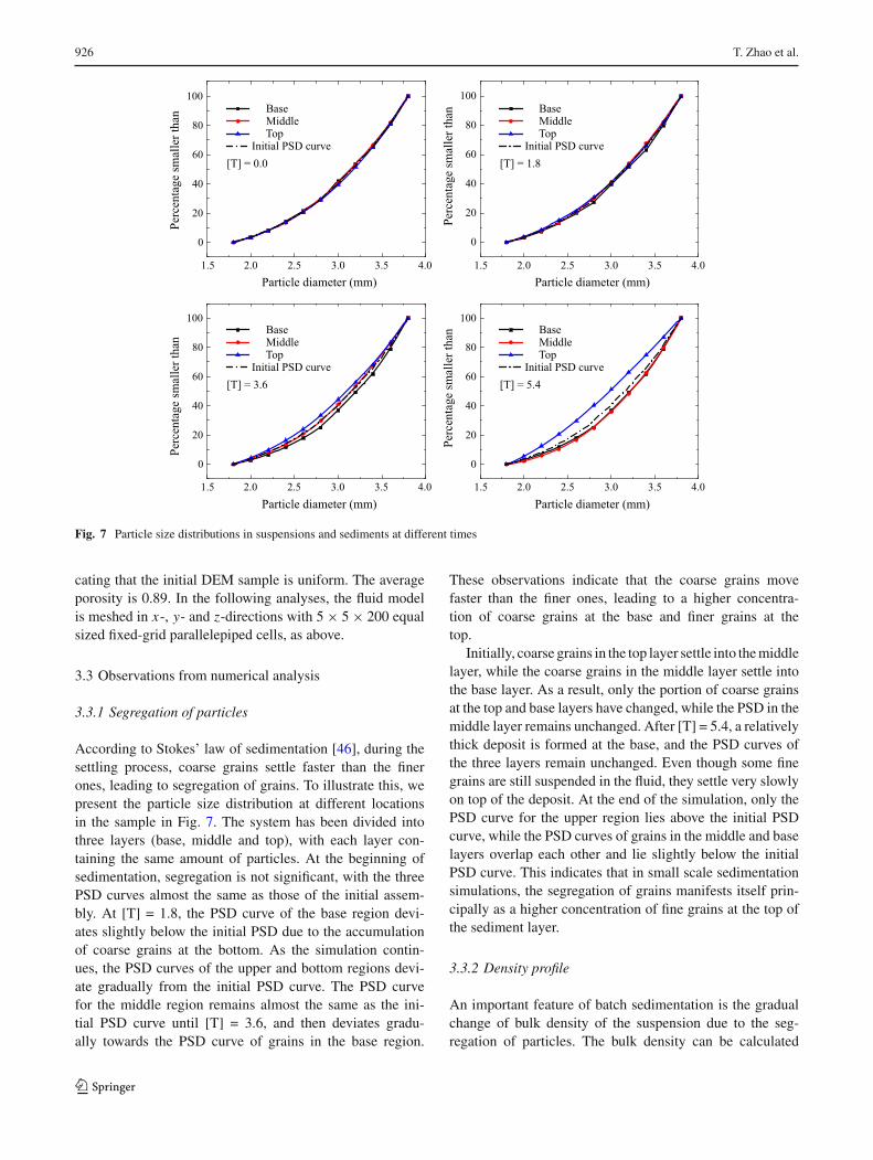
Fig. 7 Particle size distributions in suspensions and sediments at different times

cating that the initial DEM sample is uniform. The averageporosity is 0.89. In the following analyses, the fluid modelis meshed in x-, y- and z-directions with 5 × 5 × 200 equalsized fixed-grid parallelepiped cells, as above.

3.3 Observations from numerical analysis

3.3.1 Segregation of particles

According to Stokes’ law of sedimentation [46], during thesettling process, coarse grains settle faster than the finerones, leading to segregation of grains. To illustrate this, wepresent the particle size distribution at different locationsin the sample in Fig. 7. The system has been divided intothree layers (base, middle and top), with each layer con-taining the same amount of particles. At the beginning ofsedimentation, segregation is not significant, with the threePSD curves almost the same as those of the initial assem-bly. At [T] = 1.8, the PSD curve of the base region devi-ates slightly below the initial PSD due to the accumulationof coarse grains at the bottom. As the simulation contin-ues, the PSD curves of the upper and bottom regions devi-ate gradually from the initial PSD curve. The PSD curvefor the middle region remains almost the same as the ini-tial PSD curve until [T] = 3.6, and then deviates gradu-ally towards the PSD curve of grains in the base region.

These observations indicate that the coarse grains movefaster than the finer ones, leading to a higher concentra-tion of coarse grains at the base and finer grains at thetop.

Initially, coarse grains in the top layer settle into the middlelayer, while the coarse grains in the middle layer settle intothe base layer. As a result, only the portion of coarse grainsat the top and base layers have changed, while the PSD in themiddle layer remains unchanged. After [T] = 5.4, a relativelythick deposit is formed at the base, and the PSD curves ofthe three layers remain unchanged. Even though some finegrains are still suspended in the fluid, they settle very slowlyon top of the deposit. At the end of the simulation, only thePSD curve for the upper region lies above the initial PSDcurve, while the PSD curves of grains in the middle and baselayers overlap each other and lie slightly below the initialPSD curve. This indicates that in small scale sedimentationsimulations, the segregation of grains manifests itself prin-cipally as a higher concentration of fine grains at the top ofthe sediment layer.

3.3.2 Density profile

An important feature of batch sedimentation is the gradualchange of bulk density of the suspension due to the seg-regation of particles. The bulk density can be calculated

123


as:

ρb = nρ f + (1 − n) ρs (14)

where ρb is the bulk density ρs is the density of solid mate-rials.

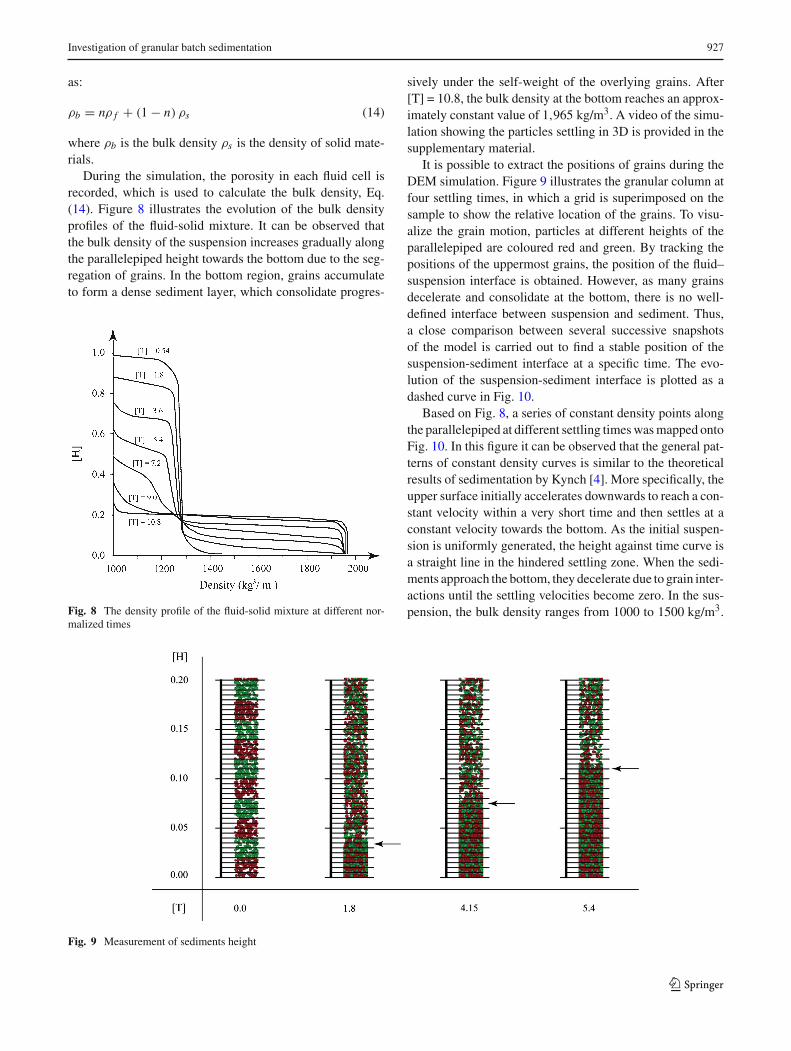
During the simulation, the porosity in each fluid cell isrecorded, which is used to calculate the bulk density, Eq.(14). Figure 8 illustrates the evolution of the bulk densityprofiles of the fluid-solid mixture. It can be observed thatthe bulk density of the suspension increases gradually alongthe parallelepiped height towards the bottom due to the seg-regation of grains. In the bottom region, grains accumulateto form a dense sediment layer, which consolidate progres-

Fig. 8 The density profile of the fluid-solid mixture at different nor-malized times

sively under the self-weight of the overlying grains. After[T] = 10.8, the bulk density at the bottom reaches an approx-imately constant value of 1,965 kg/m3. A video of the simu-lation showing the particles settling in 3D is provided in thesupplementary material.

It is possible to extract the positions of grains during theDEM simulation. Figure 9 illustrates the granular column atfour settling times, in which a grid is superimposed on thesample to show the relative location of the grains. To visu-alize the grain motion, particles at different heights of theparallelepiped are coloured red and green. By tracking thepositions of the uppermost grains, the position of the fluid–suspension interface is obtained. However, as many grainsdecelerate and consolidate at the bottom, there is no well-defined interface between suspension and sediment. Thus,a close comparison between several successive snapshotsof the model is carried out to find a stable position of thesuspension-sediment interface at a specific time. The evo-lution of the suspension-sediment interface is plotted as adashed curve in Fig. 10.

Based on Fig. 8, a series of constant density points alongthe parallelepiped at different settling times was mapped ontoFig. 10. In this figure it can be observed that the general pat-terns of constant density curves is similar to the theoreticalresults of sedimentation by Kynch [4]. More specifically, theupper surface initially accelerates downwards to reach a con-stant velocity within a very short time and then settles at aconstant velocity towards the bottom. As the initial suspen-sion is uniformly generated, the height against time curve isa straight line in the hindered settling zone. When the sedi-ments approach the bottom, they decelerate due to grain inter-actions until the settling velocities become zero. In the sus-pension, the bulk density ranges from 1000 to 1500 kg/m3.

Fig. 9 Measurement of sediments height

123

928 T. Zhao et al.

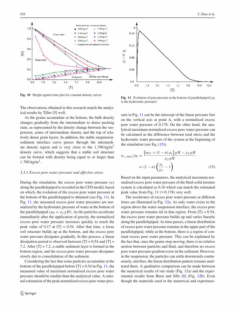
Fig. 10 Height against time plot for constant density curves

The observations obtained in this research match the analyt-ical results by Tiller [5] well.

As the grains accumulate at the bottom, the bulk densitychanges gradually from the intermediate to dense packingstate, as represented by the density change between the sus-pension, zones of intermediate density and the top of rela-tively dense grain layers. In addition, the stable suspension-sediment interface curve passes through the intermedi-ate density region and is very close to the 1,700 kg/m3

density curve, which suggests that a stable soil structurecan be formed with density being equal to or larger than1,700 kg/m3.

3.3.3 Excess pore water pressure and effective stress

During the simulation, the excess pore water pressure (u)

along the parallelepiped is recorded in the CFD model, basedon which, the evolution of the excess pore water pressure atthe bottom of the parallelepiped is obtained (see Fig. 11). InFig. 11, the measured excess pore water pressures are nor-malized by the hydrostatic pressure of water at the bottom ofthe parallelepiped (p0 = ρ f gH). As the particles accelerateimmediately after the application of gravity, the normalizedexcess pore water pressure increases quickly to reach thepeak value of 0.17 at [T] = 0.54. After that time, a loosesoil structure builds up at the bottom, and the excess porewater pressure dissipates gradually. In this process, a lineardissipation period is observed between [T] = 0.54 and [T] =7.2. After [T] = 7.2, a stable sediment layer is formed at thebottom region, and the excess pore water pressure dissipatesslowly due to consolidation of the sediment.

Considering the fact that some particles accumulate at thebottom of the parallelepiped before [T] = 0.54 in Fig. 11, themeasured value of maximum normalised excess pore waterpressure should be smaller than the analytical value. A ratio-nal estimation of the peak normalised excess pore water pres-

Fig. 11 Evolution of pore pressure at the bottom of parallelepiped (p0is the hydrostatic pressure)

sure in Fig. 11 can be the intercept of the linear pressure lineon the vertical axis at point A, with a normalized excesspore water pressure of 0.178. On the other hand, the ana-lytical maximum normalised excess pore water pressure canbe calculated as the difference between total stress and thehydrostatic water pressure of the system at the beginning ofthe simulation (see Eq. (15)).

ue_ max/p0 =[nρ f + (1 − n) ρs

]gH − ρ f gH

ρ f gH

= (1 − n)

(ρs

ρ f− 1

)(15)

Based on the input parameters, the analytical maximum nor-malised excess pore water pressure of the fluid-solid mixturesystem is calculated as 0.18 which can match the estimatedpeak value from Fig. 11 (≈0.178) very well.

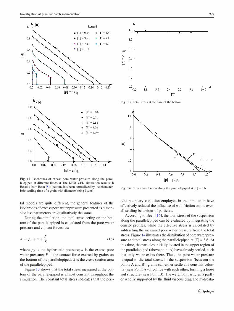
The isochrones of excess pore water pressure at differenttimes are illustrated in Fig. 12a. As only water exists in theregion above the water-suspension interface, the excess porewater pressure remains nil in that region. From [T] = 0.54,the excess pore water pressure builds up and varies linearlyalong the parallelepiped. As time passes, a linear distributionof excess pore water pressure remains in the upper part of theparallelepiped, while at the bottom, there is a region of con-stant excess pore water pressure. This can be explained bythe fact that, once the grains stop moving, there is no relativemotion between particles and fluid, and therefore no excesspore water pressure gradient exists in the sediment. However,in the suspension, the particles can settle downwards contin-uously, and thus, the linear distribution pattern remains unal-tered there. A qualitative comparison can be made betweenthe numerical results of our study (Fig. 12a) and the exper-imental results from Been and Sills [8] (Fig. 12b). Eventhough the materials used in the numerical and experimen-

123


Fig. 12 Isochrones of excess pore water pressure along the paral-lelepiped at different times. a The DEM–CFD simulation results. bResults from Been [8] (the time has been normalized by the character-istic settling time of a grain with diameter being 5 μm)

tal models are quite different, the general features of theisochrones of excess pore water pressure presented as dimen-sionless parameters are qualitatively the same.

During the simulation, the total stress acting on the bot-tom of the parallelepiped is calculated from the pore waterpressure and contact forces, as:

σ = ps + u + F

S(16)

where ps is the hydrostatic pressure; u is the excess porewater pressure; F is the contact force exerted by grains onthe bottom of the parallelepiped; S is the cross section areaof the parallelepiped.

Figure 13 shows that the total stress measured at the bot-tom of the parallelepiped is almost constant throughout thesimulation. The constant total stress indicates that the peri-

Fig. 13 Total stress at the base of the bottom

Fig. 14 Stress distribution along the parallelepiped at [T] = 3.6

odic boundary condition employed in the simulation haveeffectively reduced the influence of wall friction on the over-all settling behaviour of particles.

According to Been [16], the total stress of the suspensionalong the parallelepiped can be evaluated by integrating thedensity profiles, while the effective stress is calculated bysubtracting the measured pore water pressure from the totalstress. Figure 14 illustrates the distribution of pore water pres-sure and total stress along the parallelepiped at [T] = 3.6. Atthis time, the particles initially located in the upper region ofthe parallelepiped (above point A) have already settled, suchthat only water exists there. Thus, the pore water pressureis equal to the total stress. In the suspension (between thepoints A and B), grains can either settle at a constant veloc-ity (near Point A) or collide with each other, forming a loosesoil structure (near Point B). The weight of particles is partlyor wholly supported by the fluid viscous drag and hydrosta-

123

930 T. Zhao et al.

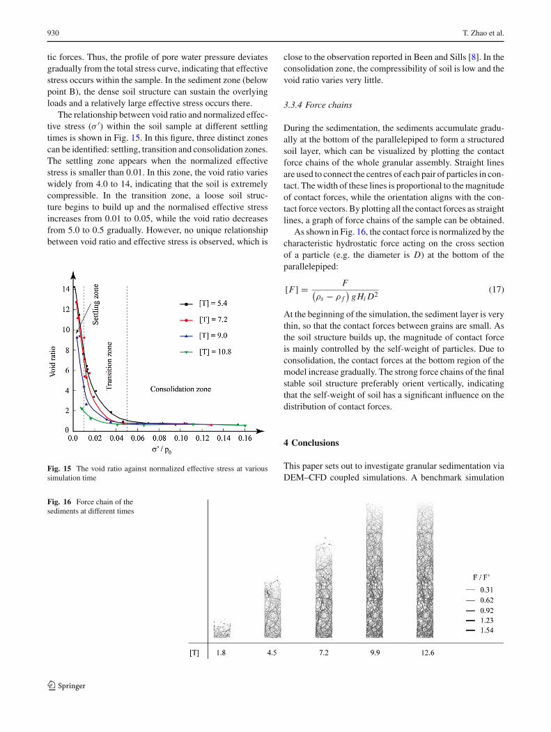
tic forces. Thus, the profile of pore water pressure deviatesgradually from the total stress curve, indicating that effectivestress occurs within the sample. In the sediment zone (belowpoint B), the dense soil structure can sustain the overlyingloads and a relatively large effective stress occurs there.

The relationship between void ratio and normalized effec-tive stress (σ ′) within the soil sample at different settlingtimes is shown in Fig. 15. In this figure, three distinct zonescan be identified: settling, transition and consolidation zones.The settling zone appears when the normalized effectivestress is smaller than 0.01. In this zone, the void ratio varieswidely from 4.0 to 14, indicating that the soil is extremelycompressible. In the transition zone, a loose soil struc-ture begins to build up and the normalised effective stressincreases from 0.01 to 0.05, while the void ratio decreasesfrom 5.0 to 0.5 gradually. However, no unique relationshipbetween void ratio and effective stress is observed, which is

Fig. 15 The void ratio against normalized effective stress at varioussimulation time

close to the observation reported in Been and Sills [8]. In theconsolidation zone, the compressibility of soil is low and thevoid ratio varies very little.

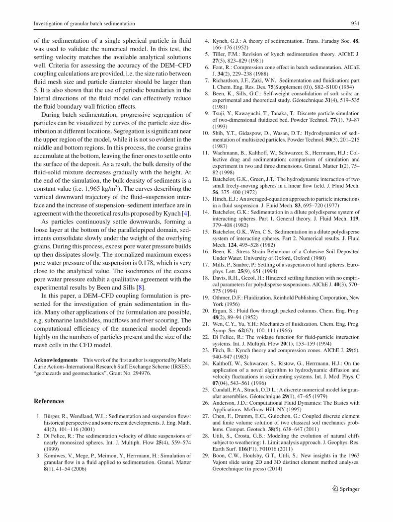
3.3.4 Force chains

During the sedimentation, the sediments accumulate gradu-ally at the bottom of the parallelepiped to form a structuredsoil layer, which can be visualized by plotting the contactforce chains of the whole granular assembly. Straight linesare used to connect the centres of each pair of particles in con-tact. The width of these lines is proportional to the magnitudeof contact forces, while the orientation aligns with the con-tact force vectors. By plotting all the contact forces as straightlines, a graph of force chains of the sample can be obtained.

As shown in Fig. 16, the contact force is normalized by thecharacteristic hydrostatic force acting on the cross sectionof a particle (e.g. the diameter is D) at the bottom of theparallelepiped:

[F] = F(ρs − ρ f

)gHi D2

(17)

At the beginning of the simulation, the sediment layer is verythin, so that the contact forces between grains are small. Asthe soil structure builds up, the magnitude of contact forceis mainly controlled by the self-weight of particles. Due toconsolidation, the contact forces at the bottom region of themodel increase gradually. The strong force chains of the finalstable soil structure preferably orient vertically, indicatingthat the self-weight of soil has a significant influence on thedistribution of contact forces.

4 Conclusions

This paper sets out to investigate granular sedimentation viaDEM–CFD coupled simulations. A benchmark simulation

Fig. 16 Force chain of thesediments at different times

123


of the sedimentation of a single spherical particle in fluidwas used to validate the numerical model. In this test, thesettling velocity matches the available analytical solutionswell. Criteria for assessing the accuracy of the DEM–CFDcoupling calculations are provided, i.e. the size ratio betweenfluid mesh size and particle diameter should be larger than5. It is also shown that the use of periodic boundaries in thelateral directions of the fluid model can effectively reducethe fluid boundary wall friction effects.

During batch sedimentation, progressive segregation ofparticles can be visualized by curves of the particle size dis-tribution at different locations. Segregation is significant nearthe upper region of the model, while it is not so evident in themiddle and bottom regions. In this process, the coarse grainsaccumulate at the bottom, leaving the finer ones to settle ontothe surface of the deposit. As a result, the bulk density of thefluid-solid mixture decreases gradually with the height. Atthe end of the simulation, the bulk density of sediments is aconstant value (i.e. 1,965 kg/m3). The curves describing thevertical downward trajectory of the fluid–suspension inter-face and the increase of suspension–sediment interface are inagreement with the theoretical results proposed by Kynch [4].

As particles continuously settle downwards, forming aloose layer at the bottom of the parallelepiped domain, sed-iments consolidate slowly under the weight of the overlyinggrains. During this process, excess pore water pressure buildsup then dissipates slowly. The normalized maximum excesspore water pressure of the suspension is 0.178, which is veryclose to the analytical value. The isochrones of the excesspore water pressure exhibit a qualitative agreement with theexperimental results by Been and Sills [8].

In this paper, a DEM–CFD coupling formulation is pre-sented for the investigation of grain sedimentation in flu-ids. Many other applications of the formulation are possible,e.g. submarine landslides, mudflows and river scouring. Thecomputational efficiency of the numerical model dependshighly on the numbers of particles present and the size of themesh cells in the CFD model.

Acknowledgments This work of the first author is supported by MarieCurie Actions-International Research Staff Exchange Scheme (IRSES).“geohazards and geomechanics”, Grant No. 294976.

References

1. Bürger, R., Wendland, W.L.: Sedimentation and suspension flows:historical perspective and some recent developments. J. Eng. Math.41(2), 101–116 (2001)

2. Di Felice, R.: The sedimentation velocity of dilute suspensions ofnearly monosized spheres. Int. J. Multiph. Flow 25(4), 559–574(1999)

3. Komiwes, V., Mege, P., Meimon, Y., Herrmann, H.: Simulation ofgranular flow in a fluid applied to sedimentation. Granul. Matter8(1), 41–54 (2006)

4. Kynch, G.J.: A theory of sedimentation. Trans. Faraday Soc. 48,166–176 (1952)

5. Tiller, F.M.: Revision of kynch sedimentation theory. AIChE J.27(5), 823–829 (1981)

6. Font, R.: Compression zone effect in batch sedimentation. AIChEJ. 34(2), 229–238 (1988)

7. Richardson, J.F., Zaki, W.N.: Sedimentation and fluidisation: partI. Chem. Eng. Res. Des. 75(Supplement (0)), S82–S100 (1954)

8. Been, K., Sills, G.C.: Self-weight consolidation of soft soils: anexperimental and theoretical study. Géotechnique 31(4), 519–535(1981)

9. Tsuji, Y., Kawaguchi, T., Tanaka, T.: Discrete particle simulationof two-dimensional fluidized bed. Powder Technol. 77(1), 79–87(1993)

10. Shih, Y.T., Gidaspow, D., Wasan, D.T.: Hydrodynamics of sedi-mentation of multisized particles. Powder Technol. 50(3), 201–215(1987)

11. Wachmann, B., Kalthoff, W., Schwarzer, S., Herrmann, H.J.: Col-lective drag and sedimentation: comparison of simulation andexperiment in two and three dimensions. Granul. Matter 1(2), 75–82 (1998)

12. Batchelor, G.K., Green, J.T.: The hydrodynamic interaction of twosmall freely-moving spheres in a linear flow field. J. Fluid Mech.56, 375–400 (1972)

13. Hinch, E.J.: An averaged-equation approach to particle interactionsin a fluid suspension. J. Fluid Mech. 83, 695–720 (1977)

14. Batchelor, G.K.: Sedimentation in a dilute polydisperse system ofinteracting spheres. Part 1. General theory. J. Fluid Mech. 119,379–408 (1982)

15. Batchelor, G.K., Wen, C.S.: Sedimentation in a dilute polydispersesystem of interacting spheres. Part 2. Numerical results. J. FluidMech. 124, 495–528 (1982)

16. Been, K.: Stress Strain Behaviour of a Cohesive Soil DepositedUnder Water. University of Oxford, Oxford (1980)

17. Mills, P., Snabre, P.: Settling of a suspension of hard spheres. Euro-phys. Lett. 25(9), 651 (1994)

18. Davis, R.H., Gecol, H.: Hindered settling function with no empiri-cal parameters for polydisperse suspensions. AIChE J. 40(3), 570–575 (1994)

19. Othmer, D.F.: Fluidization. Reinhold Publishing Corporation, NewYork (1956)

20. Ergun, S.: Fluid flow through packed columns. Chem. Eng. Prog.48(2), 89–94 (1952)

21. Wen, C.Y., Yu, Y.H.: Mechanics of fluidization. Chem. Eng. Prog.Symp. Ser. 62(62), 100–111 (1966)

22. Di Felice, R.: The voidage function for fluid-particle interactionsystems. Int. J. Multiph. Flow 20(1), 153–159 (1994)

23. Fitch, B.: Kynch theory and compression zones. AIChE J. 29(6),940–947 (1983)

24. Kalthoff, W., Schwarzer, S., Ristow, G., Herrmann, H.J.: On theapplication of a novel algorithm to hydrodynamic diffusion andvelocity fluctuations in sedimenting systems. Int. J. Mod. Phys. C07(04), 543–561 (1996)

25. Cundall, P.A., Strack, O.D.L.: A discrete numerical model for gran-ular assemblies. Géotechnique 29(1), 47–65 (1979)

26. Anderson, J.D.: Computational Fluid Dynamics: The Basics withApplications. McGraw-Hill, NY (1995)

27. Chen, F., Drumm, E.C., Guiochon, G.: Coupled discrete elementand finite volume solution of two classical soil mechanics prob-lems. Comput. Geotech. 38(5), 638–647 (2011)

28. Utili, S., Crosta, G.B.: Modeling the evolution of natural cliffssubject to weathering: 1. Limit analysis approach. J. Geophys. Res.Earth Surf. 116(F1), F01016 (2011)

29. Boon, C.W., Houlsby, G.T., Utili, S.: New insights in the 1963Vajont slide using 2D and 3D distinct element method analyses.Geotechnique (in press) (2014)

123

932 T. Zhao et al.

30. Utili, S., Crosta, G.B.: Modeling the evolution of natural cliffssubject to weathering: 2. Discrete element approach. J. Geophys.Res. Earth Surf. 116(F1), F01017 (2011)

31. Brennen, C.E.: Fundamentals of Multiphase Flow. Cambridge Uni-versity Press, Cambridge (2005)

32. Weatherley, D., Boros, V., Hancock, W.: ESyS-Particle Tutorial andUser’s Guide Version 2.1. Earth Systems Science ComputationalCentre, The University of Queensland (2011)

33. Abe, S., Place, D., Mora, P.: A parallel implementation of the latticesolid model for the simulation of rock mechanics and earthquakedynamics. Pure Appl. Geophys. 161(11–12), 2265–2277 (2004)

34. OpenCFD OpenFOAM—The open source CFD toolbox, http://www.openfoam.com/

35. Šmilauer, V., Catalano, E., Chareyre, B., Dorofeenko, S., Duriez,J., Gladky, A., Kozicki, J., Modenese, C., Scholtès, L., Sibille, L.,Stránský, J., Thoeni, K.: Yade Documentation, (The YADE Project;http://yade-dem.org/doc/) (2010)

36. Iwashita, K.: Rolling resistance at contacts in simulation of shearband development by DEM. J. Eng. Mech. 124(285), 285–292(1998)

37. Jiang, M.J., Yu, H.S., Harris, D.: A novel discrete model for gran-ular material incorporating rolling resistance. Comput. Geotech.32(5), 340–357 (2005)

38. Belheine, N., Plassiard, J.P., Donzé, F.V., Darve, F., Seridi, A.:Numerical simulation of drained triaxial test using 3D discrete ele-ment modeling. Comput. Geotech. 36(1–2), 320–331 (2009)

39. Shafipour, R., Soroush, A.: Fluid coupled-DEM modelling ofundrained behavior of granular media. Comput. Geotech. 35(5),673–685 (2008)

40. Kafui, D.K., Johnson, S., Thornton, C., Seville, J.P.K.: Paralleliza-tion of a Lagrangian–Eulerian DEM/CFD code for application tofluidized beds. Powder Technol. 207(1–3), 270–278 (2011)

41. Zeghal, M., El Shamy, U.: A continuum-discrete hydromechani-cal analysis of granular deposit liquefaction. Int. J. Numer. Anal.Methods Geomech. 28(14), 1361–1383 (2004)

42. Drew, D.A., Lahey, R.T.: Some supplemental analysis concerningthe virtual mass and lift force on a sphere in a rotating and strainingflow. Int. J. Multiph. Flow 16(6), 1127–1130 (1990)

43. DEMSolutions: EDEM-CFD Coupling for FLUENT: User Guide(2010)

44. Kafui, K.D., Thornton, C., Adams, M.J.: Discrete particle-continuum fluid modelling of gas-solid fluidised beds. Chem. Eng.Sci. 57(13), 2395–2410 (2002)

45. Guo, Y.: A coupled DEM/CFD analysis of die filling process—PhDThesis. The University of Birmingham (2010)

46. Stokes, G.G.: Mathematical and Physical Papers. Cambridge Uni-versity Press, Cambridge (1901)

47. Choi, H.G., Joseph, D.D.: Fluidization by lift of 300 circular par-ticles in plane Poiseuille flow by direct numerical simulation. J.Fluid Mech. 438, 101–128 (2001)

48. Zhang, J., Fan, L.S., Zhu, C., Pfeffer, R., Qi, D.: Dynamic behaviorof collision of elastic spheres in viscous fluids. Powder Technol.106(1–2), 98–109 (1999)

49. Beetstra, R., van der Hoef, M.A., Kuipers, J.A.M.: Drag forceof intermediate Reynolds number flow past mono- and bidispersearrays of spheres. AIChE J. 53(2), 489–501 (2007)

50. DallaValle, J.M.: Micromeritics: The Technology of Fine Particles,2nd edn. Pitman Pub. Corp (1948)

51. Brown, P., Lawler, D.: Sphere drag and settling velocity revisited.J. Environ. Eng. 129(3), 222–231 (2003)

52. Itasca: CCFD-PFC Documentaton, 1.0 vols. Itasca ConsultingGroup Inc, Minnesota (2008)

123

http://www.openfoam.com/

http://www.openfoam.com/

http://yade-dem.org/doc/

Investigation of granular batch sedimentation via DEM–CFD coupling

Documents

Transcript of Investigation of granular batch sedimentation via DEM–CFD coupling