CFD SIMULATION AND EXPERIMENTAL INVESTIGA - USQ ...
240
PERFORMANCE ENHANCEMENT OF SOLAR STILL DESALINATION SYSTEMS USING REVOLVING TUBES: CFD SIMULATION AND EXPERIMENTAL INVESTIGATION A Thesis submitted by Ahmed Kasim Taha Alkaisi M.Sc. B.Sc. Mechanical Engineering For the award of Doctor of Philosophy 2019
-
Upload
khangminh22 -
Category
Documents
-
view
3 -
download
0
Transcript of CFD SIMULATION AND EXPERIMENTAL INVESTIGA - USQ ...

PERFORMANCE ENHANCEMENT OF SOLAR STILL
DESALINATION SYSTEMS USING REVOLVING TUBES:
CFD SIMULATION AND EXPERIMENTAL INVESTIGATION
A Thesis submitted by
Ahmed Kasim Taha Alkaisi
M.Sc. B.Sc. Mechanical Engineering
For the award of
Doctor of Philosophy
2019

i
Abstract
Water and energy are indispensable resources for life and civilisation. The
scarcity of both water and energy have emerged as amongst the most serious concerns
of our time due to the dramatic growth in population, enhancement in our standards of
living, and the rapid development of the agricultural and industrial sectors in many
countries. Desalination seems to be one of the most promising solutions to solve the
problem of water scarcity; however, it is not without costs, as the desalination process
is energy-intensive. Conventional sources of energy, such as fossil fuels, are limited,
depleted and pollute the environment. Therefore, the use of renewable sources of
energy such as solar energy is essential and represents a better option. Solar
desalination systems are environmentally friendly and offer a win-win solution to
solve shortages of both water and energy. The simplest and the most straightforward
solar desalination process is the natural evaporation-condensation process of the Solar
Still Desalination (SD) system. An SD system simply consists of a water basin and a
tilted transparent cover that is exposed to solar radiation. SD systems have a low
capital cost; however, the low productivity of these systems make the cost of the water
that they produce higher than that produced via other traditional desalination systems.
On balance, the selection of SD systems for remote areas that have relatively low
demand for water makes those systems a feasible option, due to the elimination of the
high costs of water transfer if such systems are deployed locally. SD systems can work
powered by solar energy, which makes them environmentally friendly and suitable for
areas that have no access to electricity, such as remote villages and less developed
regions of the world.
The main purpose of this study is to find a method to increase the productivity
of SD systems to provide people in remote and less developed regions of the world
with freshwater. The proposed technique is a simple amendment to the regular double-
sloped SD system. The suggested modification was to add three parallel and
symmetrical PVC tubes into the water basin of the SD system to be rotated by small
DC motors. These tubes were wrapped in an absorbent black mat and were placed
horizontally along the basin to be semi immersed in the water. The purpose of this
modification is to stir the water in the basin and to generate a thin water layer around
the tubes’ circumference, which leads to an increase in the surface area for water

ii
evaporation. This modification enhanced the water evaporation rate within the SD
system, and thereby increased the productivity of this system.
In this study, two SD systems: the Normal SD (NSD) system and the Modified
SD (MSD) system were designed and manufactured, simulated numerically and tested
experimentally. The CFD simulation was done using ANSYS-Fluent software. The
experimental investigations were carried out during spring and summer in
Toowoomba, Australia. The effective operation and design parameters such as water
depth, the tubes’ diameter and the tubes’ rotation speed were analysed and optimised
using the sensitivity analysis. The dimensional analysis, uncertainty analysis, and the
cost analysis for the present experimental setup of both the SD systems were conducted
as well.
The daily productivity of the SD systems is equal to the distillate yield within
a day and the daily efficiency is equal to this productivity divided by the daily
insolation. The results show that the daily productivity and the daily efficiency of the
MSD system were always higher than that of the NSD system. According to the
experimental results, the maximum daily productivity and the maximum daily
efficiency of the MSD system were 2.908𝑙
𝑚2𝑑𝑎𝑦 and 21.01%, respectively. While the
maximum daily productivity and the maximum daily efficiency of the NSD system
were 1.685𝑙
𝑚2𝑑𝑎𝑦 and 13.12%, respectively. The maximum enhancement in the daily
productivity and the daily efficiency of the MSD system due to the modification were
74.8% and 63.4% higher than the NSD system, respectively. The results of the CFD
simulation showed a very good agreement with the data of the experimental
investigation, which means it is a successful tool for modelling SD systems. The cost
analysis of the present experimental setup estimated that the price of the water
produced by the MSD system and the NSD system is $0.57 per litre and $0.34 per
litre, respectively.

iii
Certification of Thesis
This Thesis is entirely the work of Ahmed Kasim Taha Alkaisi except where otherwise
acknowledged. The work is original and has not previously been submitted for any
other award, except where acknowledged.
Principal Supervisor: Dr Ahmad Sharifian-Barforoush
Associate Supervisor: Dr Ruth Mossad
Student and supervisors signatures of endorsement are held at the University.

iv
Acknowledgements
First, thank God for giving me health, courage, knowledge and strength to accomplish
this work.
With a deep sense of gratitude, I would like to express my deepest thanks and sincere
gratitude to my supervisors Dr Ruth Mossad and Dr Ahmad Sharifian-Barforoush, for
their invaluable help, advice, and encouragement. It has been a privilege to have
worked with them. I am sure without their guidance; this work would not have taken
this final shape.
I am indebted to all staff members at the University of Southern Queensland, special
thanks to Mr Mohan Trada, Mr Brian Aston, Mr Oliver Kinder, and Mr Brett Richards
for their assistance in the experimental setup of this project, and special thanks to Ms
Libby Collett for proofreading this thesis.
I would like to thank my sponsor the Higher Committee for Education Development
and the Ministry of Water Resources in Iraq for their financial support throughout this
research.
At last, I offer my sincere thanks to my family, my friends, and all of the people that
supported and encouraged me during the period of my study.
Ahmed Alkaisi
2019

v
Dedication
To my beloved mother with gratitude
To the memory of my dear father and my dear sister

vi
Table of Contents Abstract i
Certification of Thesis iii
Acknowledgements iv
Dedication v
Nomenclature ix
1 Chapter One: Introduction .................................................................................... 1
1.1 Background .................................................................................................... 1
1.2 Desalination Techniques ................................................................................ 3
1.2.1 Evaporation- Condensation Systems ...................................................... 3
1.2.2 Filtration Systems ................................................................................... 8
1.2.3 Crystallisation Systems ........................................................................ 10
1.3 Solar Still Desalination Systems.................................................................. 11
1.4 Cost of Desalination .................................................................................... 12
1.5 Present Study ............................................................................................... 16
1.6 Thesis Objectives ......................................................................................... 20
1.7 Thesis Outline .............................................................................................. 21
2 Chapter Two: Literature Review ........................................................................ 22
2.1 Conventional SD Systems ........................................................................... 22
2.2 Modified SD Systems .................................................................................. 24
2.2.1 SD Systems with External Heat Sources.............................................. 24
2.2.2 SD Systems with Thermal Energy Storages ........................................ 28
2.2.3 SD Systems with Reflective Surfaces .................................................. 33
2.2.4 SD Systems with External Condensers ................................................ 36
2.2.5 SD Systems with Cover Cooling .......................................................... 41
2.2.6 SD Systems with Extended Surfaces ................................................... 45
2.2.7 Other Improvements to the SD Systems .............................................. 50
2.3 SD Systems Simulation ............................................................................... 54
2.4 SD Systems Productivity and Cost .............................................................. 57

vii
2.5 Conclusions Drawn From the Literature ..................................................... 59
3 Chapter Three: CFD Simulation ........................................................................ 62
3.1 Theoretical Background .............................................................................. 62
3.2 CFD Software .............................................................................................. 67
3.3 Models Design and Mesh ............................................................................ 68
3.4 Multiphase Flows ........................................................................................ 71
3.5 Assumptions ................................................................................................ 73
3.6 Governing Equations ................................................................................... 74
3.6.1 Continuity Equation ............................................................................. 74
3.6.2 Momentum Equation ............................................................................ 74
3.6.3 Energy Equation ................................................................................... 75
3.6.4 Radiation Equation ............................................................................... 75
3.6.5 Convection Equation ............................................................................ 77
3.6.6 Turbulence Equations........................................................................... 77
3.6.7 Mass Transfer Equations ...................................................................... 79
3.7 Initial and Boundary Conditions ................................................................. 80
3.8 Solution Method .......................................................................................... 81
4 Chapter Four: Experimental Investigation ......................................................... 85
4.1 Experimental Setup ..................................................................................... 85
4.1.1 NSD system .......................................................................................... 86
4.1.2 MSD system ......................................................................................... 87
4.2 Construction Materials ................................................................................ 89
4.3 Instrumentation ............................................................................................ 91
4.4 Observation ................................................................................................. 93
4.5 Data Collection ............................................................................................ 99
5 Chapter Five: Results and Discussions ............................................................ 101
5.1 Results of the CFD Simulation .................................................................. 101

viii
5.1.1 Solar Radiation ................................................................................... 102
5.1.2 Temperature ....................................................................................... 103
5.1.3 Pressure .............................................................................................. 105
5.1.4 Density ............................................................................................... 106
5.1.5 Velocity .............................................................................................. 107
5.1.6 Evaporation and Condensation ........................................................... 108
5.2 Results of the Experimental Investigation ................................................. 110
5.2.1 Temperature Profile ............................................................................ 110
5.2.2 Productivity ........................................................................................ 113
5.2.3 Efficiency ........................................................................................... 119
5.2.4 Enhancement in Productivity and Efficiency ..................................... 124
5.2.5 Datasheets ........................................................................................... 127
5.3 Mesh Independence Study ......................................................................... 130
5.4 CFD Model Validation .............................................................................. 132
6 Chapter Six: Analyses ...................................................................................... 135
6.1 Sensitivity Analysis ................................................................................... 136
6.1.1 Regression Analysis ........................................................................... 136
6.1.2 Dimensional Analysis ........................................................................ 144
6.2 Uncertainty Analysis ................................................................................. 150
6.3 Cost Analysis ............................................................................................. 152
7 Chapter Seven: Conclusions and Recommendations ....................................... 155
7.1 Thesis Summary ........................................................................................ 155
7.2 Conclusions ............................................................................................... 156
7.3 Recommendations ..................................................................................... 158
References 159
Appendix A: Figures 173
Appendix B Tables 195
Appendix C Uncertainty Analysis Calculations 226

ix
Nomenclature
The symbols used in this thesis have the following meanings unless otherwise stated in
the text.
Symbol Description Units
𝐴 Area 𝑚2
𝐶 Constant
𝑐𝑝 Heat capacity at constant pressure 𝑘𝐽/𝑘𝑔. 𝐾
𝐸 Energy 𝑘𝐽
�� Force vector 𝑁
𝐺 Solar insolation 𝑀𝐽/𝑚2. 𝑑𝑎𝑦
𝐺𝑟 Grashof number (ratio of buoyancy forces to viscous forces) Dimensionless
�� Gravitational acceleration 𝑚/𝑠2
ℎ Heat transfer coefficient
Species enthalpy
𝑊/𝑚2. 𝐾
𝑘𝐽/𝑘𝑔
𝐼 Solar radiation intensity 𝑊/𝑚2
𝑘 Thermal conductivity
Kinetic energy of turbulence per unit mass
𝑊/𝑚. 𝐾
𝐽/𝑘𝑔
𝐿𝑣 Latent heat of evaporation 𝑀𝐽/𝑘𝑔
𝑙 Length 𝑚
𝑚 Mass 𝑘𝑔
�� Mass flow rate 𝑘𝑔/𝑠
𝑁𝑢 Nusselt number (ratio of convective to conductive heat transfer) Dimensionless
𝑝 Pressure 𝑃𝑎 = 𝑁/𝑚2
𝑃𝑟 Prandtl number (ratio of momentum diffusivity to thermal
diffusivity)
Dimensionless
𝑄 Heat 𝑊
�� Heat flux 𝑊/𝑚2
𝑅 Radius 𝑚
𝑅𝑎 Rayleigh number (strength of buoyancy in natural convection) Dimensionless
𝑅𝑒 Reynolds number (ratio of inertial forces to viscous forces) Dimensionless
𝑇 Temperature 𝐾, ℃
𝑡 Time 𝑠
𝑈 Free-stream velocity 𝑚/𝑠
𝑉 Volume 𝑚3
�� Velocity vector 𝑚/𝑠
𝑊 Work 𝐽

x
Greek symbols
Symbol Description Units
𝛼 Absorptivity
Thermal diffusivity
Dimensionless
𝑚2/𝑠
𝛽 Thermal expansion coefficient 𝐾−1
𝛥 Change in variable (𝑓𝑖𝑛𝑎𝑙 − 𝑖𝑛𝑖𝑡𝑖𝑎𝑙)
𝜀 Emissivity
Turbulent dissipation rate
Dimensionless
𝑚2/𝑠3
𝜂 Efficiency Dimensionless
𝜇 Dynamic viscosity 𝑘𝑔/𝑚. 𝑠
𝜈 Kinematic viscosity 𝑚2/𝑠
𝜌 Density 𝑘𝑔/𝑚3
𝜎 Reflectivity
Surface tension
Dimensionless
𝑘𝑔/𝑚
𝜏 Transmissivity Dimensionless
𝜔 Rotational speed 𝑟𝑝𝑚, 𝑟𝑎𝑑/𝑠
Subscripts
Symbol Description
𝑎 Ambient
𝑏 Basin
𝑐 Cover
𝑒, 𝑒𝑣 Evaporation
𝑒𝑓𝑓 Effective
𝑔 Glass
𝑘 Conduction
𝑙 Liquid
𝑟 Radiation
𝑠 Storage, Solar, Surface
𝑡 Total
𝑣 Vapour
𝑤 Water
∞ Freestream
xi
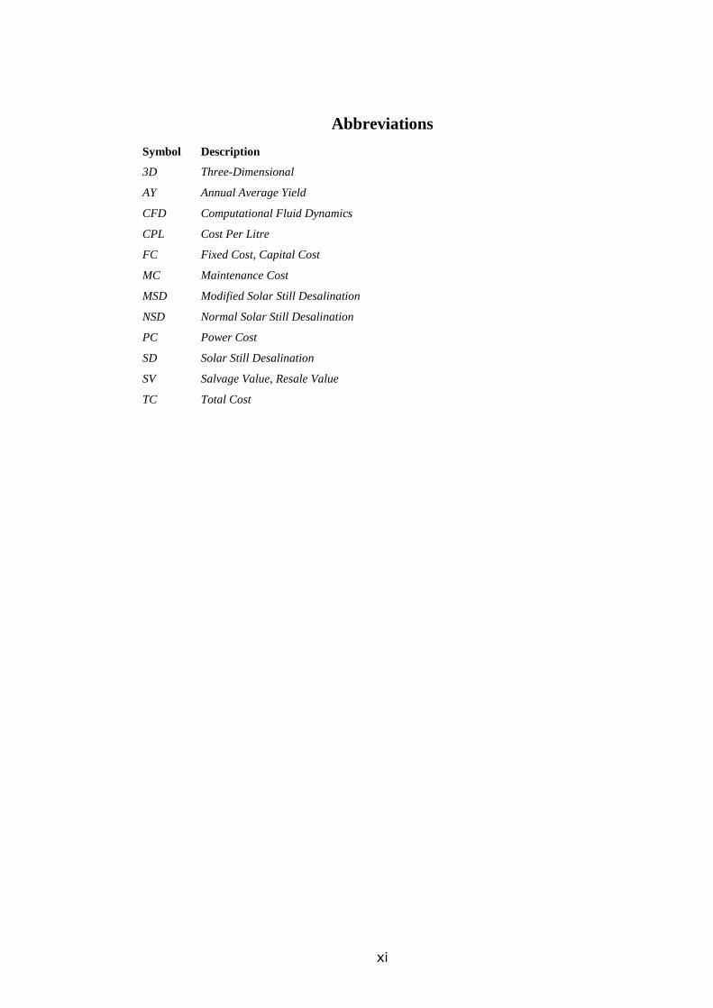
Abbreviations
Symbol Description
3D Three-Dimensional
AY Annual Average Yield
CFD Computational Fluid Dynamics
CPL Cost Per Litre
FC Fixed Cost, Capital Cost
MC Maintenance Cost
MSD Modified Solar Still Desalination
NSD Normal Solar Still Desalination
PC Power Cost
SD Solar Still Desalination
SV Salvage Value, Resale Value
TC Total Cost

Chapter 1 Introduction
1
1 Chapter One: Introduction
Water means life. Freshwater is an essential element not only to human life but also to
almost all human daily activities such as domestic uses and hygiene, livestock farming,
crop irrigation, and most industrial processes. Without freshwater, humans cannot
survive or exist.
1.1 Background
Despite the fact that water covers about 75% of the earth’s surface area, freshwater
represents only about 2.5% of the total amount of global water stores and the rest is
saline water (Eakins & Sharman, 2010). Moreover, not all of the 2.5% is an accessible
resource, as most of the freshwater is in the form of groundwater, permafrost, glaciers,
and ice caps; and only about 0.007% is accessible surface freshwater such as that
stored in lakes and rivers (Gleick, 1993). Figure 1.1 shows by percentages the
distribution of water globally (Perlman, 2016).
Figure 1. 1 Global water distribution (Perlman, 2016)

Chapter 1 Introduction
2
Water can be classified into four categories according to its salt contents (from fresh
to salty) into; freshwater, brackish water, seawater, and brine. Freshwater is defined as
water with a total dissolved salts/solids (TDS) level of fewer than 500 parts per million
(ppm) or (mg/l), while brackish water has a TDS of up to 7000 ppm, seawater has a
TDS of up to 35000 ppm and beyond salinity level, water is considered to be brine
(Lethea, 2017). According to the World Health Organisation (2011), the best quality
of drinking water has less than 300 ppm, but the permissible limit of salinity in potable
water is up to 1000 ppm.
Water scarcity is the most crucial issue of our time. Water scarcity occurs when water
supplies fall below 1000 cubic meters per capita per year and absolute scarcity occurs
when the water supplies are below 500 cubic meters per capita per year (Rijsberman,
2006). Freshwater is an unsustainable resource due to overexploitation, contamination,
weather changes, and global warming. Furthermore, the population explosion, the
increase in living standards and their consequential results such as the growth in the
industrial and the agricultural sectors have worsened the problem of the water scarcity.
According to a recent report by the World Health Organization and UNICEF (2017),
844 million people do not have sufficient freshwater.
To overcome the water shortage problem, many plans and solutions have been applied
such as building dams and reservoirs, recycling and reusing greywater (wastewater),
harvesting rainwater, and seawater desalination. However, there are some negative
impacts caused by the afore-mentioned solutions. The main disadvantages of the use
of dams and reservoirs are that they use of large areas of land that could otherwise be
used for agricultural, industrial or residential activities, as well as the high capital cost.
Meanwhile there are public health issues that have held back the widespread use of
recycled and reused wastewater. Seawater desalination is one of the most promising
techniques in producing freshwater; however, seawater desalination is an energy-
intensive process, which also creates environmental pollution. Employing renewable
energy sources into the seawater desalination process can mitigate the environmental
issues of desalination and can reduce the cost of producing freshwater significantly
(Shatat et al, 2013).

Chapter 1 Introduction
3
1.2 Desalination Techniques
Desalination is defined simply as the process of producing freshwater from saline
water. Desalination techniques can be categorized into three main groups: evaporation-
condensation, filtration, and crystallisation. Figure 1.2 presents the different
techniques of desalination under these three main groups.
Figure 1. 2 Desalination techniques
1.2.1 Evaporation- Condensation Systems
In these systems, freshwater is obtained by evaporating the saline water then
condensing the vapour to produce pure water. These systems produce freshwater with
TDS up to 20 ppm, which is considered to be high-quality purification. The following
are the most common evaporation-condensation techniques:

Chapter 1 Introduction
4
a) Multi-Effect Distillation (MED): In this process, the saline water is heated by
solar energy or fossil fuels and sprayed in parallel vacuumed vessels to
decrease the evaporation temperature. The latent heat rejected by the produced
vapour in the condensation process is used to preheat the feed saline water.
This method is commonly used in oil-rich countries because it requires heat
from burning fuel or with the aid of solar energy more than electric power.
Figure 1.3 shows a schematic diagram of a MED system with a solar water
heater (Sharaf et al, 2011).
Figure 1. 3 Schematic diagram of the MED system (Sharaf et al, 2011)
b) Multi-Stage Flash Desalination (MSF): Saline water in the MSF system is
heated by burning fuel or with the help of solar radiation under high pressure
to increase the boiling temperature and then the water is pumped into low-
pressure vessels to produce vapour. The formed vapour on the condenser tubes
preheats the feed saline water. This system is also widely used in Middle-
Eastern and oil-rich countries for the same reason mentioned in the previous
paragraph (section a). Figure 1.4 shows a schematic diagram of the MSF
system with a solar heater and heat storage (Moustafa et al, 1985).

Chapter 1 Introduction
5
Figure 1. 4 Schematic diagram of the MSF system (Moustafa et al, 1985)
c) Mechanical Vapour Compression (MVC): In this system, a mechanical
compressor is used to increase the vapour pressure and temperature. The
compressed hot vapour is used to heat up the saline water to produce more
vapour. The compressed vapour is then condensed under high temperature, and
the latent heat of condensation is used to preheat the feed water. Figure 1.5
shows a schematic diagram of a single stage MVC system (Helal & Al-Malek,
2006).
Figure 1. 5 Schematic diagram of the MVC system (Helal & Al-Malek, 2006)

Chapter 1 Introduction
6
d) Thermal Vapour Compression (TVC): In this system, a thermo-compressor
is used to increase the steam pressure, which leads to enhancing the
desalination performance due to increase in the condensation temperature and
the vapour can be used as a heating medium to the feedwater. Figure 1.6 shows
a schematic diagram of the TVC system combined with MED system (Yang et
al, 2015).
Figure 1. 6 Schematic diagram of the TVC system (Yang et al, 2015)
e) Natural Vacuum Desalination: The main idea of this system is to produce
vapour at low water temperature. Whilst water can evaporate at low
temperature under vacuum pressure, producing vacuum pressure requires a
complex system and a huge amount of energy. In natural vacuum desalination
systems, the saline water is pumped to a certain height and let it flow down
under its weight and gravity, which produces a vacuum pressure that is required
for the evaporation at low temperature. The main advantage of this process is
the low power consumption. However, this method has limited productivity
(Maroo & Goswami, 2009). Figure 1.7 shows a schematic diagram of a simple
natural vacuum desalination system with a solar heater as a booster
enhancement (Al-Kharabsheh & Yogi, 2003).

Chapter 1 Introduction
7
Figure 1. 7 Schematic diagram of the Natural vacuum desalination system (Al-Kharabsheh & Yogi, 2003)
f) Humidification-Dehumidification Desalination (HDH): As implied by the
name, HDH is a system that combines two chambers, one for evaporation and
one for condensation. There are four types of HDH systems; open water- open
air, closed water- closed air, closed water- open air, and open water- closed air
cycles (Parekh et al, 2004). The fact that hot air can carry more moisture is
employed in the HDH systems. Therefore, heated air is circulated in the system
using an external source of energy. In addition, the heat rejected from the
vapour is used to heat up the feed saline water in sequence processes by
employing a hot air circulation. Figure 1.8 shows a schematic diagram of a
simple HDH system in four configurations with solar air and water heaters
(Parekh et al, 2004).

Chapter 1 Introduction
8
Figure 1. 8 Schematic diagram of the HDH system (Parekh et al, 2004)
1.2.2 Filtration Systems
In these systems, the saline water is pumped at high pressure through many stages of
filters to purify the water from the suspended solids and dissolved salts. The total
dissolved solids TDS of the water produced depends on the system type, size, pressure
and the number of filtration stages. Most of these systems produce freshwater with
TDS up to 500 ppm, which is an acceptable limit for human consumption. The
following are the most common filtration techniques:
a) Reverse Osmosis (RO): RO is a widespread common technique used around
the world, especially in the western developed countries, due to the fact that it
consumes energy more efficiently compared with thermal systems. RO system
is a pressure-driven desalination process in which the feedwater is pumped to

Chapter 1 Introduction
9
a pressure that is higher than the osmotic pressure of the membranes. The cross-
flow membrane unit allows water molecules to pass through, leaving behind
the bigger particles of the salt and other solids. The water processed in multi-
stages until reaching a desirable TDS, usually in the range of 500 ppm to 700
ppm. The feed water is usually pre-treated to remove all impurities, and the
freshwater produced is post-treated to be potable water. Figure 1.9 shows the
basic elements of the RO system (Australian Water Association, 2009).
Figure 1. 9 Schematic diagram of the RO system (Australian Water Association, 2009)
b) Forward Osmosis (FO): FO is a new technique that allows the saline water to
move naturally using osmotic pressure instead of applying a hydraulic pressure
as in the RO systems. The seawater moves through a semipermeable membrane
into a highly concentrated solution of ammonia salts leaving the sea salts on
another side. This technique consumes less power than RO; however, this
method requires more research and development (Akther, 2015).

Chapter 1 Introduction
10
c) Electro-Dialysis (ED): The seawater is composed of negative ions called
anions and positive ions called cations. When DC polarity is applied across the
cathode and anode the feed water converts it into two streams; concentrated
brine and freshwater. The negative ions pass through the anion exchange
membrane and positive ions pass through the cation exchange membranes and
these ions get accumulated in a certain compartment and are cleared out as a
brine, while freshwater passes through the other passages (Sadrzadeh &
Mohammadi, 2008).
d) Nano Filtration (NF): Nano-filtration is a recently developed membrane
filtration technique that relies on the permeability of membranes to distinguish
between the physical size and the type of the particles in mixtures or in
solutions. NF works under low pressure and is mainly used for water post-
treatment and food processing (Hirunpinyopas, 2017).
e) Membrane Distillation (MD): MD is a separation process in which only
vapours are allowed to pass through a porous hydrophobic membrane. It is a
new desalination technique that is still under development. It combines both
the evaporation-condensation and filtration processes (Wang & Chung, 2015).
1.2.3 Crystallisation Systems
In these methods, a salt separation occurs due to molecular crystallisation. Freshwater
can be produced by removing the formed salts or the concentrated brine. The following
are the most common methods:
a) Freezing: In this process, a pure water ice crystal grows on the saline water
surface leaving concentrated brine. The freshwater is achieved by separating
the ice from the concentrated brine. The main advantages of this system are
that the energy required for freezing is less than that required for evaporation.
In addition, ice has a less corrosive effect on the system materials than vapour.
The disadvantages of this method are the inherent complexities of the
refrigeration systems and the ice separation mechanisms. In addition, this

Chapter 1 Introduction
11
process requires freshwater to wash the produced ice before melting (Qiblawey
& Banat, 2008).
b) Hydration: This is an old fashioned chemical-based desalination process
employing a gas hydrate such as methane, carbon dioxide or nitrogen to
remove the dissolved minerals from the seawater such as Na, K, Mg2, Ca, B,
Cl, and SO4 (Kang et al, 2014).
1.3 Solar Still Desalination Systems
The Solar Still Desalination (SD) system is a simple device that has a low cost and low
maintenance. The SD simply consists of a blackened basin covered with an inclined
transparent cover. The working principle of the SD system is simple and it relies on
the phenomenon of evaporation and condensation as well as gravity. The blackened
basin and the brackish water in it absorb the solar energy that transmits through the
transparent cover, which produces water vapour due to the increase in the water
temperature. The water vapour condenses on the tilted cover, producing freshwater
that trickles down into the discharge channel. Figure 1.10 shows a schematic diagram
of a conventional SD system (Sharshir et al, 2016).
Figure 1. 10 A schematic diagram of the conventional single-slope SD system (Sharshir et al, 2016)

Chapter 1 Introduction
12
The SD systems can be divided - according to its operation method - into passive and
active types. The passive SD systems typically depend only on solar energy and do not
require any mechanical parts or the use of any other sources of energy, while the active
SD systems require an external source of energy to run special mechanical equipment
such as pumps and fans. The SD system also can be sorted according to the cover
shape into single-slope, double-slope, pyramidal, conical, hemispherical or tubular
cover SD system or according to the basin to single basin, stepped basin, or multi-
basin SD system. Most SD systems have the advantages of being cheap, simple, and
do not require special skills or maintenance. It can be run by inexperienced people,
and it is environmentally friendly. The only drawback of the SD systems is the low
productivity per unit area which is about (2-3) litres per meter square per day
(Qiblawey & Banat, 2008).
1.4 Cost of Desalination
Over the last few decades, systematic research and development have reduced the cost
of desalination technology due to more efficient designs, lower power requirement,
and higher water productivity. According to the International Desalination Association
(IDA), more than 86.8 million cubic meters per day are produced by 18,426
desalination plants that are installed in over 150 countries to provide more than 300
million people with fresh water daily (Baawain et al, 2015). Figure 1.11 shows the
desalination capacity of some countries with production size over 70,000 cubic meters
per day (Peluffo & Neger, 2013).

Chapter 1 Introduction
13
Figure 1. 11 The global desalination capacity (Peluffo & Neger, 2013)
The contribution of each desalination technique to the world water production is as
follows; about 62% is the RO systems production, about 24% is the MED and MSF
systems production, and about 14% desalinated water is produced by other
desalination techniques as shown in the figure 1.12 (Ghaffour et al, 2015). The RO
systems are the most applicable in the western countries because they are electrically
driven and more energy-efficient than other desalination systems while, the MED and
MSF systems are the most common desalination techniques in the oil-rich countries
because these systems depend on the heat produced from burning fuel which is
abundant in these countries.

Chapter 1 Introduction
14
Figure 1. 12 The contribution of each desalination technique by percentages (Ghaffour et al, 2015)
The impact of the desalination on the environment is the production of greenhouse
gases, and these gases are regarded as being the main cause of global warming.
Desalination using the above methods is power-intensive process in which, to produce
1,000 cubic meters per day of freshwater requires about 10,000 tons of oil per year
(Shatat et al, 2013). Therefore, it is not easy to estimate the exact cost of the
desalination process or the cost of freshwater produced by the desalination techniques
due to the hidden environmental factor as well as fluctuating oil prices. However, the
availability and the cost of the energy and the feedwater, the workforce wages, the
maintenance cost, the land cost, and the government subsidy are the main factors,
which play a significant role in estimating the cost of the water produced by the
desalination technology.
In general, the total cost of desalination can be divided into three main categories;
about 45-50% is the capital investment repayment, about 33-49% is the cost of the
electrical and/or thermal energy, and about 6-17% is the operational and maintenance
cost. Figure 1.13 shows the percentage of the total annual cost of the main desalination
techniques (Huttner, 2013).

Chapter 1 Introduction
15
Figure 1. 13 The total annual cost percentage of the main desalination systems (Huttner, 2013)
The cost of the water produced by desalination systems can be lowered significantly
by increasing the size/scale of production; which means that the bigger desalination
plants are more economical and feasible than the smaller ones. However, in the remote
areas, a small desalination plant is feasible due to the high cost of water transport
(Gude et al, 2010). Table 1.1 lists the cost of freshwater produced by some desalination
systems.
Table 1. 1 The cost of the water produced by the main desalination technologies
Desalination
systems
Capacity
(m3/day)
Energy source Cost
(USD/m3)
Reference
SD 1 Solar 12 (Banat & Jwaied, 2008)
SD 5 Solar 3 (Goosen et al, 2000)
RO 10 Electrical 14 (Banat & Jwaied, 2008)
RO 250 Electrical 3.2 (Slesarenko, 2001)
RO 500 Electrical 2.6 (Rayan et al, 2001)
RO 2000 Electrical 2.2 (Lamei et al, 2008)
ED 10 Electrical 5 (Banat & Jwaied, 2008)
MED 100 Thermal 5.5 (Karagiannis & Soldatos, 2008)
MSF 20,000 Thermal 2 (Banat & Jwaied, 2008)
MVC 375 Thermal and
electrical
3.8 (El-Mudir et al, 2004)

Chapter 1 Introduction
16
1.5 Present Study
The SD system is the most appropriate technique for remote and rural areas,
whose populations are suffering from water and energy stress. SD systems are simple,
could be portable, provide a reasonable amount of potable water, and the most
important feature of these systems is that they could solely run on solar energy, hence
they are environmentally friendly. The only disadvantage of the SD systems is their
low productivity, which makes it a costly and unfeasible choice for areas experiencing
high demand for water. However, in scenarios with a small scale of water demand such
as on small islands, ships, villages, or even for household use, the use of the SD system
is a competitive option due to the high cost of other methods of acquiring water such
as water transportation or connection to the electricity grids.
The low productivity of the SD systems has motivated researchers to try to
improve the performance of those systems. Numerous researchers had proposed
several modifications and improvements to the SD systems to enhance the systems’
performance and to increase the water production of those systems. However, most of
these modifications and improvements to the SD systems led to an increase in costs
and/or complexities of those systems, and/or a failure to achieve significant
augmentation in water productivity. Therefore, further research is required to produce
an SD system with higher productivity, whilst maintaining simplicity and low cost.
Some examples of the previous efforts to enhance the performance of the SD systems
(all mentioned in details in chapter two) are: increasing the temperature of the
feedwater using heat exchangers and heaters (Kumar et al, 2014); storing the solar
energy using thermal storages (Kabeel & Abdelgaied, 2017); increasing the solar gain
using reflectors (Estahbanati et al, 2016); increasing the condensation rate using
vacuum fans and separated condensers (El-Samadony et al, 2015); decreasing the
temperature of the cover using film cooling (Sharshir et al, 2017); and increasing the
surface area of the water using fins (Srivastava & Agrawal, 2013).
The main aim or purpose of this research is finding ways to improve the
productivity of the SD systems - using a simple and low-cost technique - to make them
available to a wide range of beneficiaries, especially to those living in remote and
arid/semi-arid areas, and poorer/less-developed regions. From previous research that
was found in the literature review, extending the surface area of the water seems to be

Chapter 1 Introduction
17
promising. Since the evaporation occurs on the free surface of the water that is in
contact with the ambient air, increasing the water surface area will lead to an increase
in the evaporation rate, which will enhance the productivity of the SD systems.
Another finding from the literature review that - as implied by the name of the Solar
“Still” Desalination system - the water in these systems is usually “still” or “stagnant”;
and most previous studies of the SD systems deal with water that is stagnant in the
basins of these systems.
The research gap is how combining two ideas for enhancements will affect the
performance of the system; for instance, extending the water surface area and
generating water movement within the basin of the SD system. The research question
then is: what are the effects of stirring the water and increasing the surface area of the
water on the SD system’s performance and productivity? To achieve this goal,
revolving tubes have been introduced into the water basin of the SD system to produce
water circulation around the tubes’ circumference and to extend the surface area the
water. Three symmetrical PVC tubes were proposed to be semi-immersed into the
water basin of the SD system. These tubes placed horizontally in a parallel
arrangement and coupled with small DC motors to generate the rotational movement.
These tubes have the advantages of stirring the water, extending the surface area of the
water, and absorbing solar radiation as well. This amendment or modification to the
SD system will hopefully increase the water evaporation rate, and thereby, enhance
the SD system performance and productivity.
In this study, two SD systems will be run at the same time under the same
weather conditions in Toowoomba, Australia during two seasons, spring and summer.
The first system is a regular or normal double-sloped SD system that is denoted by
(NSD) and the second system is the modified SD system with the proposed revolving
tubes that is denoted by (MSD). Both the SD systems will have the same dimensions
and are made of the same construction materials, except for the modification of the
revolving tubes in the MSD system. Figures 1.14 and 1.15 show sketches of the two
SD systems; the MSD and the NSD under study.

Chapter 1 Introduction
18
Figure 1. 14 A schematic diagram of the NSD system under study
Figure 1. 15 A schematic diagram of the MSD system under study

Chapter 1 Introduction
19
The methodology of this research is conducting numerical simulation and
experimental investigations for both SD systems. The numerical simulation will be
done by developing a CFD model with the aid of ANSYS-Fluent software. The
experimental investigations will be done by manufacturing two physical small-scale
models to meet with the research budget. Comparisons will be done between these two
SD systems. The sensitivity analysis (optimisation) to the design parameters such as
water depth, tube diameter, tube rotation speed, the dimensional analysis, the
uncertainty analysis of the measured values, and the cost analysis of both the SD
systems will be conducted as well.
The significance of this research is its contribution to engineering and health
sectors. Water, energy, and the environment are amongst the most vital factors
affecting our life and wellbeing. We all need clean and safe water, sustainable and
green energy, and an environment that is free of contaminants to survive and thrive.
Traditional desalination techniques that use fossil fuels produce greenhouse gases that
pollute the environment and worsen the problem of global warming. Moreover, fossil
fuels are finite and will soon run out. Using solar energy in desalination has become
essential to mitigate the effect of using fossil fuels. Solar desalination provides a clean
and sustainable solution to the problems of both energy and water scarcity. The
availability of fresh and safe water without the need for using traditional energy
sources has great significance and high levels of impact on the economy, society,
environment, health, and human life. Another significance of this research is the
provision of a device at low cost, that is simple to maintain, easy to run, and
environmentally friendly for water desalination purposes that will be available to a
wide range of people, especially for those living in remote and arid areas and poor
people living in less-developed countries with few resources. This system can sustain
communities in those areas and has the potential to revive abandoned remote lands.
Other important outcomes of this study are to provide researchers with knowledge of
the effect of combining these enhancement ideas and provide the designers with a
simple optimisation to some important parameters of designing SD systems. If the
suggested modification to the SD system achieves a good enhancement in producing
freshwater, it can be manufactured in larger scales to provide a wide range of
beneficiaries with reasonably priced freshwater.

Chapter 1 Introduction
20
1.6 Thesis Objectives
The objectives of the present research are as follows:
1. Designing the NSD system, which is a conventional double-slope SD system
depending on the current knowledge that is available in the literature; then
design the MSD system including the proposed modification of three revolving
tubes in its basin.
2. Developing a CFD model to simulate numerically the NSD system and the
MSD system using ANSYS-Fluent software.
3. Manufacturing moderate-sized NSD and MSD systems.
4. Conducting experimental investigations for both the SD systems over two
seasons; spring and summer in Toowoomba, Australia.
5. Estimating the uncertainty analysis of the measured values.
6. Validating the results of the CFD simulation using the experimental data.
7. Implementing a sensitivity analysis (optimisation) of the operation and design
parameters for both the SD systems using the developed CFD model.
8. Conducting a dimensional analysis of the parameters that affect the
productivity of the SD systems.
9. Performing a cost analysis of the present experimental setup of both the SD
systems.
10. Presenting and discussing the results, reaching conclusions, and suggesting
recommendations for future work.

Chapter 1 Introduction
21
1.7 Thesis Outline
The following is a brief description of the structure or an overview of this thesis;
1. Chapter One: Introduction: Gives a brief background of the current water
status and the water desalination techniques. States the research problem and
suggests a possible solution. Presents the research aim, the research gap, the
research question, the research methodology, and the significance of the study.
Outlines the objectives of this project.
2. Chapter Two: Literature Review: Presents the existing knowledge and the
current efforts undertaken by the researchers in developing the SD systems.
Reaches conclusions that will help in identifying the research gap and
developing the aim of the present research.
3. Chapter Three: CFD Simulation: Presents the theoretical background and
the correlations that were used to estimate the productivity and the efficiency
of the SD system. The chapter presents the governing partial differential
equations and highlight the assumptions used to facilitate the solution. It
describes the steps that were taken to conduct the numerical simulation such as
creating the geometry and generating the computational grid. Then it presents
the numerical models that were used in this study and the solution method.
4. Chapter Four: Experimental Investigation: Describes the experimental
setup of both the SD systems that were used in this project and presents the
instrumentation, observation, and data collection.
5. Chapter Five: Results and Discussion: Presents and discusses the results of
the CFD simulation and the recorded data from the experimental investigations
and makes a comparison between both SD systems under study. Validates the
CFD results with the experimental data.
6. Chapter Six: Analyses: Presents the important analyses that were done in this
study, the sensitivity analysis (optimisation) of the operation and design
conditions, the dimensional analysis to the parameters that affect the
productivity, the uncertainty analysis, and the cost analysis of both the SD
systems under study.
7. Chapter Seven: Conclusions and Recommendations: Presents a summary
of the thesis, reaches conclusions and provides suggestions for future work.

Chapter 2 Literature Review
22
2 Chapter Two: Literature Review
This chapter presents recent efforts done by researchers to enhance the performance
of the Solar Still Desalination (SD) systems and the recent developments applied to
SD systems found in the literature. This chapter is divided into the following sections;
firstly it presents the conventional SD systems, then the enhancements that were
introduced to the SD systems, then the previous numerical simulation of the SD
systems, then the water productivity and its cost by the SD systems, and finally the
conclusions drawn from the literature review.
2.1 Conventional SD Systems
The conventional SD system refers to the regular and prevalent Solar Still Desalination
system without modifications or enhancements. Some researchers have studied the
conventional SD systems to understand the working principle of the SD system and
the effect of the weather, designs, and operations factors on SD systems’ performance.
Al-Hinai et al (2002) studied the effect of some weather conditions and design
parameters on the productivity of a double-slope SD system using a mathematical
model. They used a simple energy balance approach to estimate the heat transfer
coefficient of evaporation, and hence the productivity of the SD system. They found
that higher hourly productivity can be achieved with a higher solar intensity, a higher
ambient temperature, a higher wind velocity, a greater cover’s slope-angle during
winter and a steeper cover’s slope-angle during summer, a thicker basin’s insulation,
a higher feedwater temperature, and shallower water. The results showed that the
average annual productivity was (4.15 kg/m2.day) and the average cost was ($16.3
USD/m3). Figure 2.1 shows a schematic diagram of the SD system.

Chapter 2 Literature Review
23
Figure 2. 1 The schematic diagram of the SD system and the heat balance. Where: I= solar incidence, q= heat
transfer, and the subscript: abs= absorbed, c= convection, ev = evaporation, k= conduction, r = radiation,
x=stored, while w-b= the direction from water to basin, w-g= from water to glass, and g-a= from glass to
ambient (Al-Hinai et al, 2002)
Jamil and Akhtar (2017) investigated experimentally the effect of the gap between the
basin and the cover of a single-slope SD system. The fixed design parameters were;
(0.7m× 1.4m) of the basin’s dimensions, (28°) of the cover’s slope-angle (which is the
same latitude angle of the location), and (10 mm) of the water depth. They controlled
the height of the gap between the basin and the cover using polystyrene sheets within
five stages and it was from 0.266m to 0.366m. They concluded that a smaller cavity
(the gap between the basin and the cover) increases the SD system productivity.
According to the results, the average daily productivity ranged from 1.341 L/m2 to
4.186 L/m2, the average daily efficiency ranged from 11.25% to 39.59%, and the
average cost of the produced water ranged from ($0.074 USD/L) to ($0.024 USD/L).
Figure 2.2 shows a schematic diagram of the experimental setup.

Chapter 2 Literature Review
24
Figure 2. 2 The schematic diagram of the experimental setup where the polystyrene sheets used to adjust the
height between the basin and the cover, T= temperature, and the subscript b= basin, w= water, v = vapour, gi=
glass inner, go= glass outer (Jamil & Akhtar, 2017)
2.2 Modified SD Systems
Numerous researchers have introduced many types of enhancements or modifications
to the conventional SD system. Improving water productivity (the distillate yield) of
the SD systems was the main purpose of these enhancements. This section presents
the literature, which is divided according to the type of enhancement to the SD system
as follows;
2.2.1 SD Systems with External Heat Sources
One enhancement to the SD systems is by combining a further heat source to the
conventional SD system. Some researchers attempted to increase the SD systems’
productivity by accelerating the evaporation rate. For this purpose, they combined the
basin of the SD system with a sort of heat exchanger to heat up the brackish water in
the basin or to heat up the feed water pre-accessing the SD system. The external heat

Chapter 2 Literature Review
25
source could be a solar collector, solar pond, or any other waste heat source such as
the rejected heat of an engine’s exhaust system.
Badran and Al-Tahaineh (2005) investigated experimentally the effect of coupling a
flat plate solar collector with a single-slope SD system to heat up the brackish water
into the SD basin. They found that productivity of the SD system increased by (36%)
due to this modification. Figure 2.3 shows a schematic diagram of the experimental
setup and Figure 2.4 shows the variation of the hourly productivity of the conventional
and the enhanced SD systems.
Figure 2. 3 The schematic diagram of the experimental setup (Badran & Al-Tahaineh, 2005)
Figure 2. 4 The hourly productivity of the conventional and the enhanced SD systems (Badran & Al-Tahaineh,
2005)

Chapter 2 Literature Review
26
Abdel-Rehim and Lasheen (2007) combined the SD system with a solar parabolic
trough with a focal pipe and a simple heat exchanger with oil as working fluid to heat
up the brackish water in the SD basin. They found that the productivity of the SD
system increased by an average of (18%) due to the modification. Figure 2.5 shows a
schematic diagram of the experimental setup and Figure 2.6 shows the variation of the
accumulative productivity of the conventional and the modified SD systems.
Figure 2. 5 The schematic diagram of the experimental setup (Abdel-Rehim & Lasheen, 2007)
Figure 2. 6 The hourly accumulative productivity of the conventional SD system (without heater) and modified
SD system (with heater) in mL on 5/6/2005 (Abdel-Rehim & Lasheen, 2007)

Chapter 2 Literature Review
27
El-Sebaii et al (2008) studied the effect of coupling the SD system with a shallow solar
pond by a tube heat exchanger to heat up the brackish water before it gets into the SD
basin. They found that productivity and efficiency of the modified SD system were
higher by (52.36%) and (43.8%), respectively. The daily productivity of the modified
SD system ranged from (1.904 kg/m2) in winter to (6.570 kg/m2) in summer. Figure
2.7 shows a schematic diagram of the experimental setup.
Figure 2. 7 The schematic diagram of the experimental setup (El-Sebaii et al, 2008)
Kumar et al (2014) integrated a single-slope SD system with an evacuated tube solar
collector to heat up the brackish water as it goes into the SD basin. They found that
during a typical summer day, the maximum daily yield was (3.47 kg/m2) which is
higher than a conventional SD system by about (20%). The result also showed that the
maximum efficiency was (33.8%), which is higher approximately (26%) than the SD
system without this enhancement. They also concluded that the optimum water depth
into the basin is (0.03 m). Figure 2.8 shows a schematic diagram of the experimental
setup.

Chapter 2 Literature Review
28
Figure 2. 8 The schematic diagram of the experimental setup (Kumar et al, 2014)
2.2.2 SD Systems with Thermal Energy Storages
Another improvement to the SD systems is made by adding heat storage to the SD
system. Some researchers tried to store the heat of solar energy during the daytime
sunlight hours to produce more freshwater during the night and the cloudy weather,
i.e. during the absence of sunlight. For this purpose, they used many types of materials
such as rubber, rocks, marbles, etc. as sensible heat storage or Phase Change Materials
(PCM) such as paraffin wax as latent heat storage.
El-Sebaii et al (2009) investigated theoretically only the effect of adding a PCM to a
single-slope SD system. Using 3.3 cm thickness of stearic acid PCM underneath the
SD absorber surface on a typical summer day, they found that the maximum daily
productivity was (9.005 kg/m2) and (4.998 kg/m2) of the SD system with, and without
PCM, respectively. The improvement in daily productivity was about 80% due to the
enhancement of adding the PCM. Figure 2.9 shows a schematic diagram of the SD
system with the PCM.

Chapter 2 Literature Review
29
Figure 2. 9 The schematic diagram of the experimental setup (El-Sebaii et al, 2009)
Shalaby et al (2016) studied experimentally the effect of using Paraffin wax PCM
under a v-corrugated solar absorber of a single- slope SD system. They found that
using the paraffin wax PCM as latent heat storage decreases the productivity of the SD
system during the daylight by (7.4%) while increases the productivity by (72.7%)
overnight. The total daily productivity of the SD system was about (11.7%) higher
when using PCM than without PCM. Figure 2.10 shows a schematic diagram of the
experimental setup.
Figure 2. 10 The schematic diagram of the experimental setup (Shalaby et al, 2016)

Chapter 2 Literature Review
30
Dashtban and Tabrizi (2011) studied experimentally a weir-type cascade SD system
with paraffin wax PCM underneath the solar absorber surface. They found that daily
productivity of the SD system increased by (31%) when using PCM. The daily yield
was (6.7 kg/m2) and (5.1 kg/m2) for the SD system with and without PCM,
respectively. The overall thermal efficiency was 64% and 47% of the SD system with
and without PCM, respectively. Figure 2.11 shows a schematic diagram of the
experimental setup.
Figure 2. 11 The schematic diagram of the experimental setup (Dashtban & Tabrizi, 2011)
Kabeel and Abdelgaied (2016) improved the daily productivity of the SD system from
(4.51 l/m2) to (7.54 l/m2) by using PCM (Paraffin wax) layer beneath the absorber
surface of the SD system. The productivity of the SD system with PCM was higher by
(67.18%) than the SD system without PCM. Kabeel and Abdelgaied (2017) also
performed experimental tests to a modified SD system with two enhancements, a PCM
as a latent heat energy storage and an oil heat exchanger to heat the feed water. They
found that the maximum freshwater productivity was (4.48 l/m2.day) and (10.77
l/m2.day) of the conventional and the modified SD systems, respectively. The result
also showed that the maximum daily efficiency was 25.73% and 46% for the
conventional and the enhanced SD system respectively. The enhancement in the

Chapter 2 Literature Review
31
productivity and efficiency were about (140.4%) and (44%) due to the modifications,
respectively. Figure 2.12 shows a schematic diagram of the experimental setup.
Figure 2. 12 The schematic diagram of the experimental setup (Kabeel & Abdelgaied, 2017)
Murugavel et al (2010) investigated the effect of using different materials as sensible
heat storages on the SD system performance. They tested adding different types of
materials such as; quartzite rock, red brick pieces, cement concrete pieces, washed
stones, and iron scraps into the water basin of a double-slope SD system. The
dimensions of the basin were 2.08m×0.84m and the water depth in the basin was (0.5
- 0.75 cm). The results showed that the maximum enhancement in daily productivity
was 6.2% using 0.75 inches sized quartzite rock as sensible heat storage. Figure 2.13
shows the variation in the hourly productivity of the SD system using different
materials into its water basin and Figure 2.14 shows the materials that were used in
this study.

Chapter 2 Literature Review
32
Figure 2. 13 The variation in the hourly productivity of the SD system using different materials into its water
basin as sensible heat storage (Murugavel et al, 2010)
Figure 2. 14 The material used in the experimental investigation (Murugavel et al, 2010)

Chapter 2 Literature Review
33
2.2.3 SD Systems with Reflective Surfaces
Another improvement to the SD systems is by adding internal and/or external sunlight
reflectors. Some researchers tried to increase the solar radiation gain by attaching
reflector surfaces inside the basin and/or over the cover of the SD system. Increasing
the solar radiation gain means increasing the water temperature, which leads to
accelerating the evaporation rate, hence increase the productivity of the SD system.
Tanaka and Nakatake (2006) studied theoretically the effects of adding internal and
external reflectors on the SD system performance. They concluded that the annual
distillate productivity increases by an average of (48%) higher than the SD system
without reflectors. Figure 2.15 shows the schematic diagram of the modified SD
system.
Figure 2. 15 The schematic diagram of the experimental setup (Tanaka & Nakatake, 2006)
Khalifa and Ibrahim (2009) studied experimentally the effect of the internal reflectors,
the external reflector, and the inclination angle of the external reflector during all
seasons on the SD system productivity. They found that the average enhancement in
the annual productivity was (19.9%) with internal reflectors only and (34.4%, 34.5%,
34.8%, and 24.7%) for combined internal and external reflectors at (0°, 10°, 20°, and
30°) slope angle of the external reflector, respectively higher than the SD system

Chapter 2 Literature Review
34
without reflectors. They also concluded that the effect of the reflectors was negative
during summer. Figure 2.16 shows the schematic diagram of the experimental setup.
Figure 2. 16 The schematic diagram of the experimental setup (Khalifa & Ibrahim, 2009)
Estahbanati et al (2016) compared theoretically and experimentally the distillate
productivity of the SD system with and without internal reflectors. The results showed
that average (annual, winter, and summer) enhancement in the productivity of the SD
system with reflectors on all inner walls were (34%, 65%, and 22%) higher than the
SD system without reflectors, respectively. They also concluded that the internal
reflectors are more beneficial during winter than in summer.
Omara et al (2014) investigated the performance of a stepped basin SD system with
and without internal and external reflectors and compared it to a conventional SD
system. The results showed that the daily productivity of the stepped basin SD system
was higher than the conventional SD system by (57%, 75%, and up to 125%) when it
was without reflectors, with internal reflectors only, and with internal and external
reflectors, respectively. The daily efficiency of the conventional SD system, stepped
without reflectors SD system, and stepped with reflectors SD system were 34%, 53%,
and 56%, respectively. Figure 2.17 shows the schematic diagram of the experimental

Chapter 2 Literature Review
35
setup and Figure 2.18 shows the variation in productivity between the conventional
and modified SD systems.
Figure 2. 17 The schematic diagram of the experimental setup (Omara et al, 2014)
Figure 2. 18 The accumulative productivity of the conventional and enhanced SD systems (Omara et al, 2014)

Chapter 2 Literature Review
36
2.2.4 SD Systems with External Condensers
Another improvement to the SD system is by adding an external condenser to the
conventional SD system to increase the yield of the SD system. The idea is to cool
down the produced vapour, which leads to speed up the condensation rate hence
increase the productivity of the SD system. Combining the SD system with an external
condenser will increase the thermal efficiency of the SD system as well. However, this
modification to the SD systems requires more land area in addition to the increase in
the system capital and operation cost, complexity and further maintenance
requirements.
Abu-Qudais and Othman (1996) compared the performance of two SD systems, with
and without an external condenser. They found that the thermal efficiency of the SD
system is higher by (47%) when using the external condenser modification. Figure
2.19 shows a schematic diagram of the experimental setup.
Figure 2. 19 The schematic diagram of the experimental setup (Abu-Qudais & Othman, 1996)

Chapter 2 Literature Review
37
El-Bahi and Inan (1999a) examined experimentally attaching an outside passive
condenser and external reflector to a single-slope SD system with (4°) minimum
cover’s slope angle. They found that the maximum daily productivity of the modified
SD system was about (7 l/m2). The daily yield and the efficiency of the enhanced SD
system were improved by about (70%) and (75%), respectively. Figure 2.20 shows a
schematic diagram of the experimental setup.
Figure 2. 20 The schematic diagram of the experimental setup (El-Bahi & Inan, 1999)
Monowe et al (2011) proposed a new design of the SD system for domestic purposes
with two enhancements: an external reflector and external condenser. The results
showed that the efficiency of the proposed SD system was up to (77%) when using the
latent heat of condensation to preheat the feed brackish water (in the condenser). The
daily water productivity was up to (8 l/m2). Figure 2.21 shows a schematic diagram of
the experimental setup.

Chapter 2 Literature Review
38
Figure 2. 21 The schematic diagram of the experimental setup (Monowe et al, 2011)
Kabeel et al (2014a) investigated three enhancements to the conventional single-slope
SD system. The enhancements included adding an external condenser, adding
Nanoparticles into the water, and adding a vacuum fan. The results showed that the
daily productivity of the enhanced SD system compared to the conventional SD system
improved by (53.2%) when using the external condenser only, by (76%) when using
the external condenser and the nanoparticles into the water, and up to (116%) when
using the external condenser, the nanoparticles, and the vacuum fan. The advantage of
the vacuum fan is to extract and accelerate the humid-air flow from the SD system to
the condenser. Figure 2.22 shows a schematic diagram of the experimental setup.

Chapter 2 Literature Review
39
Figure 2. 22 The schematic diagram of the experimental setup (Kabeel et al, 2014)
El-Samadony et al (2015) modified a stepped SD system by adding an external
condenser and internal and external reflector surfaces. They compared the modified
model with a conventional single-slope SD system and they found that the productivity
was higher by (66%) when using external condenser only and by (165%) when using
the external condenser and the internal and external reflectors. Figure 2.23 shows a
schematic diagram of the experimental setup and Figure 2.24 shows the variation of
the accumulative productivity between the conventional and the modified SD systems.

Chapter 2 Literature Review
40
Figure 2. 23 The schematic diagram of the experimental setup (El-Samadony et al, 2015)
Figure 2. 24 The accumulative productivity of the conventional and the enhanced SD systems (El-Samadony et al,
2015)
Ibrahim et al (2015) investigated the effect of attaching an external condenser to a
single-slope SD system working under vacuum pressure. The result showed that the
productivity of the enhanced model was higher by (16.2%) than the conventional SD
system. The daily efficiency was (29% and 37.6%) for the conventional and the

Chapter 2 Literature Review
41
enhanced SD systems, respectively. Figure 2.25 shows a schematic diagram of the
experimental setup.
Figure 2. 25 The schematic diagram of the experimental setup (Ibrahim et al, 2015)
2.2.5 SD Systems with Cover Cooling
Another enhancement to the SD systems is by cooling down the cover of the SD
system to increase the condensation rate. Some researchers increased the distillate
yield of the SD system by lowering the temperature of the SD system cover using
many techniques.
Gupta et al (2016) investigated experimentally the effect of attaching a water sprinkler
with a constant discharge of (0.0001 kg/s) over the glass cover of a single-slope SD
system. The dimensions of the SD system were; the basin= (1×1×0.1 m), the water
depth= (5 cm), and the cover slope angle= (23°) which is equal to the latitude angle of
the experiment location. The results showed an increase in daily productivity and the
efficiency of the enhanced SD system by (20%) and (21%), respectively. The daily
productivity was (2.940 l/m2) and (3.541 l/m2) for the conventional and the enhanced
SD systems, respectively.

Chapter 2 Literature Review
42
Somwanshi and Tiwari (2014) used cool water from a tank of an air cooler to flow
over the cover of a single-slope SD system. According to the experimental data, the
productivity and the efficiency of the SD system improved by (56.5%) and (9.9%),
respectively. The results showed that the optimum flow rate of the cooling water over
the cover of the SD system was (0.075 kg/s). Figure 2.26 shows the schematic diagram
of the experimental setup.
Figure 2. 26 The schematic diagram of the experimental setup (Somwanshi & Tiwari, 2014)
Sharshir et al (2017) investigated and compared the effects of four modifications on
the performance of a single-slope SD system. The modifications were namely (A, B,
C, and D) included: (A) adding nanoparticles (flake graphite) into the water, (B)
adding nanoparticles plus PCM, (C) adding nanoparticles with cover cooling, and (D)
adding nanoparticles plus PCM with cover cooling. The purpose of adding the
nanoparticles into water is to increase the solar radiation absorbance and the thermal
conductivity of the water, the PCM is to store latent heat thermal energy, and the cover
film cooling is to decrease the cover temperature. The results showed improvement in
the productivity of the SD system by (50.28% for the model A), (65% for the model
B), (56.15% for the model C), and by (73.8% for the model D). Figure 2.27 shows the
schematic diagram of the experimental setup.

Chapter 2 Literature Review
43
Figure 2. 27 The schematic diagram of the experimental setup (Sharshir et al, 2017)
Rahbar and Esfahani (2012) introduced a heat-pipe heat exchanger as surface cooler
to the SD system. They tested their system experimentally for five days and they
concluded that the maximum daily efficiency was 70% and the system has a potential
for further developments. Figure 2.28 shows the schematic diagram of the
experimental setup and Figure 2.29 shows the productivity and efficiency of the
modified SD system.

Chapter 2 Literature Review
44
Figure 2. 28 The schematic diagram of the experimental setup (Rahbar & Esfahani, 2012)
Figure 2. 29 The hourly variation of climatic conditions, productivity, and instantaneous efficiency in a typical
day (8/2/2010) (Rahbar & Esfahani, 2012)

Chapter 2 Literature Review
45
2.2.6 SD Systems with Extended Surfaces
Another improvement to the SD systems is by adding further surfaces in the water
basin to increase the surface area of the evaporation hence enhance the evaporation
rate. The idea behind this modification is also to increase the amount of the absorbed
solar energy in addition to increasing the surface area of the evaporation, which leads
to improving the SD system productivity. For this purpose, researchers used many
kinds of extended surfaces such as; different kinds of fins, corrugated plates, perforated
plates, wicks, wire meshes etc.
Omara et al (2011) studied experimentally the effect of adding fins and corrugated
plate to the water basin of a single-slope SD system. The dimensions of the SD system
were (0.5 m×2 m) and the water depth was (50 mm). The result showed that adding
fins and corrugated plate into the basin of the SD system improved productivity by
(40%) and (21%), respectively. Figure 2.30 shows the schematic diagram of the
experimental setup and Figure 2.31 shows the accumulative yields for the different
configurations of the SD system.
Figure 2. 30 The schematic diagram of the experimental setup (Omara et al, 2011)

Chapter 2 Literature Review
46
Figure 2. 31 The accumulative productivity of the conventional and enhanced SD systems (Omara et al, 2011)
Nafey et al (2002) studied experimentally the effect of adding a floating perforated
black aluminium plate into the water basin of the SD system at different water depth
(3, 4, 5, and 6 cm). The results showed that this enhancement was more effective with
higher water depth. The distillate yield of the enhanced SD system was greater than
the conventional SD system by up to (15%) at a water depth of (3 cm), and up to (40%)
at a water depth of (6 cm).
Srivastava and Agrawal (2013a) used a floating water absorber porous material
(blackened jute cloth) to increase the evaporation surface area. The results showed that
the distillate yield of the SD system increased due to this enhancement by about (68%)
and (35%) during clear days and cloudy days, respectively. They also investigated the
effect of adding external reflectors and they achieved up to (79%) increase in
productivity due to both enhancements; i.e. the floating absorber and the external
reflectors. The results also showed that the depth of the water in the basin of the SD
system had a slight effect on productivity when using the floating absorber. Figure
2.32 shows the schematic diagram of the experimental setup and Figure 2.33 shows
the effect of the water depth in the basin of the SD system.

Chapter 2 Literature Review
47
Figure 2. 32 The schematic diagram of the experimental setup (Srivastava & Agrawal, 2013a)
Figure 2. 33 The effect of the water depth in the basin of the enhanced SD system (Srivastava & Agrawal, 2013a)
Srivastava and Agrawal (2013b) also studied the effect of adding porous fins that
extended from the base of the water basin to over the water surface on the SD
performance. The porous fins made of blackened cotton rag. The results showed that
the daily productivity of the enhanced SD system was higher by (15%) during May
(summer) and by (48%) during February (winter) compared to the conventional SD
system. The maximum achieved productivity was (7.5 kg/m2) during May. Figure 2.34
shows the schematic diagram of the experimental setup and Figure 2.35 shows the
accumulated productivity of the conventional and modified SD system during a typical
day of winter and summer seasons.

Chapter 2 Literature Review
48
Figure 2. 34 The schematic diagram of the experimental setup (Srivastava & Agrawal, 2013b)
Figure 2. 35 The accumulative productivity of the modified and the conventional SD systems during summer
(May) and winter (February) 2012 (Srivastava & Agrawal, 2013b)
Abu-Hijleh and Rababa'h (2003) investigated the effect of adding black coal, yellow
sponge cubes, black sponge cubes, and black steel cubes into the water basin of the
SD system. The results showed an increase in the SD system productivity about (18%
- 73%) and the black sponge cubes was the most effective. The tested SD system
dimensions were; the basin = (0.5×0.5 m), the cover slope angle = (23°), and the water
depth (50 mm). Figure 2.36 shows the schematic diagram of the experimental setup.

Chapter 2 Literature Review
49
Figure 2. 36 The schematic diagram of the experimental setup (Abu-Hijleh & Rababa'h, 2003)
Sakthivel et al (2010) studied the effect of using jute cloth to extend the evaporation
surface area. According to the results, the maximum improvement in the daily
productivity of the modified SD system compared to the conventional SD system was
(20%), and the maximum daily efficiency of the modified SD system was (52%),
which was higher than the conventional SD system by (8%). Figure 3.37 shows the
schematic diagram of the experimental setup.
Figure 2. 37 The schematic diagram of the experimental setup (Sakthivel et al, 2010)

Chapter 2 Literature Review
50
2.2.7 Other Improvements to the SD Systems
Abdallah and Badran (2008) employed a sun tracking system to enhance SD system
productivity. They used a simple single-slope single basin SD system with the
dimensions of (1m×1.2 m) and (32°) of the cover tilt angle. The results showed that
the sun tracking system improved the daily productivity of the SD system by about
(22%) higher than the fixed SD system. Figure 2.38 shows the difference in the hourly
productivity of both the SD systems.
Figure 2. 38 The variation in the hourly productivity between the fixed and sun tracked SD systems (Abdallah &
Badran, 2008)
Kianifar et al (2012) investigated the effect of adding fan inside a pyramid-shaped
cover SD system. They found that during the summer season, the productivity of the
SD system increased by (20%) due to using the fan, while the fan had an unnoticeable
effect during the winter season. Figure 2.39 shows the schematic diagram of the
experimental setup.

Chapter 2 Literature Review
51
Figure 2. 39 The schematic diagram of the experimental setup (Kianifar et al, 2012)
Dev et al (2011a & 2011b) introduced an inverted absorber SD system and compared
its performance to a conventional SD system. The results showed that the maximum
daily productivity was (6.3 kg/m2) and (4.15 kg/m2) for the inverted SD system and
the conventional SD system, respectively. The results also showed that the maximum
daily efficiency was (34.6%) and (48%) for the inverted SD system and the normal SD
system, respectively. They also studied the effect of the water depth, and they found
that the optimal water depth was (3 cm). Figure 2.40 shows the schematic diagram of
the experimental setup.

Chapter 2 Literature Review
52
Figure 2. 40 The schematic diagram of the experimental setup (Dev et al, 2011b)
El-Agouz (2014) tested a single-slope stepped basin SD system with water circulation
using a water pump. The results showed that the productivity of the modified SD
system was higher than the conventional SD system by up to (48%), and the daily
efficiency was higher by about (20%). Figure 2.41 shows the schematic diagram of the
experimental setup.
Figure 2. 41 The schematic diagram of the experimental setup. (1) Solar still frame, (2) glass cover, (3) absorber
plate, (4) digital thermometer, (5) water vessel, (6, 12) control valve, (7) water drain, (8) graduate level, (9) flow
meter, (10) water pump and (11) control timer (El-Agouz, 2014)

Chapter 2 Literature Review
53
Al-Sulttani et al (2017) tested a Double-slope SD system with rubber scrapers on the
cover inner-surface. The rubber scrapers are similar to windshield wiper blades. The
purpose of the rubber scrapers is to collect the condensed water on the inner surface
of the cover of the SD system allowing more light (solar energy) to be transmitted and
preventing the condensed water from re-evaporating. The results showed that the
average daily productivity was (4.24 l/m2) and the productivity enhancement was
about (63%) due to using the rubber scrapers enhancement. Figure 2.42 shows the
schematic diagram of the experimental setup and Figure 2.43 shows the accumulated
productivity of the conventional and the modified SD systems.
Figure 2. 42 The schematic diagram of the experimental setup (Al-Sulttani et al, 2017)

Chapter 2 Literature Review
54
Figure 2. 43 The accumulative productivity of the conventional and modified SD systems (Al-Sulttani et al, 2017)
2.3 SD Systems Simulation
Due to the complexity of the evaporation-condensation phenomena involved in the SD
systems, most previous work on the SD systems were experimental investigations.
Only a few researchers had conducted a numerical simulation of the SD systems.
Setoodeh et al (2011) used CFD software (ANSYS CFX 11) to simulate the
evaporation-condensation processes in a single-slope SD system to estimate the
evaporation flow rate. For that purpose, they employed the volume of fluid (VOF)
multiphase model with two phases; the water-liquid phase and the water-vapour phase.
They did not include a turbulence model as they assumed a low evaporation rate. In
addition, they assumed a steady-state condition, and they employed a quasi-steady
analysis with constant temperature boundary conditions. They concluded that CFD is
a powerful tool for the purpose of simulation and parametric analysis of SD systems.
Figure 2.44 shows the contour of the water distribution on the cover of the SD system.

Chapter 2 Literature Review
55
Figure 2. 44 The contour of the water volume fraction on the cover of the SD system (Setoodeh et al, 2011)
Rashidi et al (2018) employed a two-phase flow model using (ANSYS fluent) solver
to simulate the evaporation-condensation problem occur in the SD system. They used
the VOF multiphase model in two-dimensional (2D) geometry under steady state
condition. The boundary conditions were; no heat flux from the walls, and constant
temperature of 30° and 40° for the glass cover and the absorber plate, respectively.
They did not include the solar radiation effect nor the turbulence flow. Figure 2.45
shows the contour of the water volume fraction in the SD system.
Figure 2. 45 The contour of the water volume fraction in the SD system (Rashidi et al, 2018)

Chapter 2 Literature Review
56
Rahbar and Esfahani (2013) examined the capability of a two-dimensional simulation
using ANSYS Fluent CFD software to estimate the SD system productivity. They
compared the results of the CFD simulation with a well-known correlation (Dunkle’s
model) for the estimation of the daily yield of the SD system. They concluded that the
CFD simulation was a successful tool to estimate the productivity of the SD system
and in a good agreement with the available experimental results. They used steady-
state, laminar flow, and assumed that the vapour is an incompressible ideal gas. For
the boundary conditions, they assumed adiabatic walls and constant temperature for
the cover and the bottom. Figure 3.46 shows the vapour mass fraction contour lines.
Figure 2. 46 The vapour mass fraction contour lines of the SD system (Rahbar & Esfahani, 2013)
Rahbar et al (2015) also investigated the distillate yield of a tubular SD system using
CFD simulation. They employed two-dimensional analysis in (ANSYS fluent 14) CFD
software. They assumed laminar flow, steady-state, and constant properties for the
water and the vapour. The boundary conditions assumed to be constant temperature
for the water and the vapour and adiabatic walls. They concluded that the accuracy of
the results of the CFD simulation was about ±15% compared to the previous
experimental work.
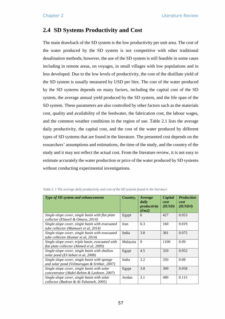
Chapter 2 Literature Review
57
2.4 SD Systems Productivity and Cost
The main drawback of the SD system is the low productivity per unit area. The cost of
the water produced by the SD system is not competitive with other traditional
desalination methods; however, the use of the SD system is still feasible in some cases
including in remote areas, on voyages, in small villages with low populations and in
less developed. Due to the low levels of productivity, the cost of the distillate yield of
the SD system is usually measured by USD per litre. The cost of the water produced
by the SD systems depends on many factors, including the capital cost of the SD
system, the average annual yield produced by the SD system, and the life span of the
SD system. These parameters are also controlled by other factors such as the materials
cost, quality and availability of the feedwater, the fabrication cost, the labour wages,
and the common weather conditions in the region of use. Table 2.1 lists the average
daily productivity, the capital cost, and the cost of the water produced by different
types of SD systems that are found in the literature. The presented cost depends on the
researchers’ assumptions and estimations, the time of the study, and the country of the
study and it may not reflect the actual cost. From the literature review, it is not easy to
estimate accurately the water production or price of the water produced by SD systems
without conducting experimental investigations.
Table 2. 1 The average daily productivity and cost of the SD systems found in the literature
Type of SD system and enhancements Country, Average
daily
productivity
(l/m2)
Capital
cost
($USD)
Production
cost
($USD/l)
Single-slope cover, single basin with flat plate
collector (Eltawil & Omara, 2014)
Egypt 6 427 0.053
Single-slope cover, single basin with evacuated
tube collector (Mamouri et al, 2014)
Iran 6.3 160 0.019
Single-slope cover, single basin with evacuated
tube collector (Kumar et al, 2014)
India 3.8 381 0.075
Single-slope cover, triple basin, evacuated with
flat plate collector (Ahmed et al, 2009)
Malaysia 9 1100 0.09
Single-slope cover, single basin with shallow
solar pond (El-Sebaii et al, 2008)
Egypt 4.5 320 0.052
Single-slope cover, single basin with sponge
and solar pond (Velmurugan & Srithar, 2007)
India 3.2 350 0.08
Single-slope cover, single basin with solar
concentrator (Abdel-Rehim & Lasheen, 2007)
Egypt 3.8 300 0.058
Single-slope cover, single basin with solar
collector (Badran & Al-Tahaineh, 2005)
Jordan 3.1 480 0.115

Chapter 2 Literature Review
58
Type of SD system and enhancements Country, Average
daily
productivity
(l/m2)
Capital
cost
($USD)
Production
cost
($USD/l)
Single-slope cover, single basin with fins and
solar pond (Appadurai & Velmurugan, 2015)
India 3 310 0.076
Single-slope cover, single basin with fins
(Velmurugan et al, 2008a)
India 2.8 200 0.054
Single-slope cover, single basin with fins and
wick (Velmurugan et al, 2008b)
India 2.8 250 0.065
Single-slope cover, single basin with PCM and
wick (Shalaby et al, 2016)
Egypt 3.3 238 0.095
Single-slope cover, single basin with PCM
(Kabeel & Abdelgaied, 2016)
Egypt 3.5 165 0.032
Single-slope cover, single basin with PCM
(Ansari et al, 2013)
Morocco 3 245 0.06
Single-slope cover, Stepped basin with pebbles
(Velmurugan et al, 2009)
India 3.3 160 0.072
Single-slope cover, Stepped basin with
reflectors (Omara et al, 2014)
Egypt 5.1 240 0.031
Single-slope cover, single basin, vacuum with
external condenser (Ibrahim et al, 2015)
Egypt 2.5 195 0.041
Single-slope cover, single basin, nanoparticles
with external condenser and vacuum fan
(Kabeel et al, 2014b)
Egypt 6 268 0.022
Double-glass cover, single basin with separate
condenser (El-Bahi & Inan, 1999b)
Turkey 4.3 350 0.06
Single-slope cover, single basin with cover
cooling (Rahbar & Esfahani, 2012)
Iran 4.1 181 0.27
Hemispherical cover with cover cooling
(Arunkumar et al, 2012)
India 4.2 165 0.041
Single-slope cover, single basin with fins and
corrugated plate (Omara et al, 2011)
Egypt 3.5 122 0.03
Pyramidal cover, concave basin with wick
(Kabeel, 2009)
Egypt 4.1 145.5 0.065
Triangular cover (Ahsan et al, 2014) Malaysia 4.1 35 0.017
Tubular cover (Ahsan et al, 2012) Japan 5 355 0.105
Hemispherical cover (Ismail, 2009) Canada 4 958 0.18
Pyramidal cover (Fath et al, 2003) Egypt 2.9 99.5 0.016
Single-slope cover, stepped basin with water
circulation (El-Agouz, 2014)
Egypt 5.2 300 0.035
Single-slope cover, single basin with inverted
absorber (Dev et al, 2011b)
Oman 4 165 0.031
Single-slope cover, single basin with sun
tracking (Abdallah & Badran, 2008)
Jordan 1.25 282 0.167
Single-slope cover, Stepped basin with sun
tracking (Abdallah et al, 2008)
Jordan 3.7 350 0.071

Chapter 2 Literature Review
59
2.5 Conclusions Drawn From the Literature
After conducting an intense literature review of numerous previous studies on the Solar
Still Desalination (SD) Systems, the following conclusions were drawn:
1. Due to the complexity of the evaporation-condensation phenomena involved
in the SD systems, most previous research on the SD systems were
experimental investigations, very few studies were theoretical or mathematical
models based upon experimental correlations, and far fewer studies used
numerical methods such as CFD simulation. In this study, both CFD simulation
and experimental investigations will be conducted to compare the results and
to evaluate the performance of the SD systems. The present study will test the
reliability of the numerical simulation and the possibility of using it for the
purpose of optimisation. The experimental investigation is essential to estimate
the cost of the SD systems and the price of the water produced by those
systems. The experimental investigation is also important and necessary to
validate the computational results.
2. Since the productivity of the SD systems is low, the purpose of most of the
previous research was to increase the distillate yield or the productivity of the
SD systems. Improving the SD systems’ productivity was achieved by many
means as follows:
i. Increase the evaporation rate: this was done using four methods; by
increasing the brackish water temperature using heaters, solar
collectors, and heat exchangers, or by extending the surface area of the
evaporation using fins and wicks, or by increasing the solar gain using
reflector surfaces, or by storing the solar heat using storage materials.
ii. Increase the condensation rate: this was done using two approaches;
by decreasing the cover temperature using film cooling, or by using an
external condenser.
iii. Enhance the thermo-optical properties of brackish water: by
adding dyes and/or nanoparticles to improve the thermal conductivity
and the solar radiation absorption of the brackish water
iv. Some researchers combined two or more enhancements to the SD
system or introduced new designs such as multi-stage SD systems.

Chapter 2 Literature Review
60
3. According to the literature review, extending the evaporation surface
enhancement to improve the productivity of the SD systems seems to be a
promising enhancement and it will be employed in this research. Since the
evaporation occurs from the water surface, extending the surface area of the
evaporation enhances the productivity of the SD system.
4. According to the literature review, most previous studies were for SD systems
with stagnant or still water in their basins. In the current study, a rotational
movement will be introduced to the water in the basin of the SD system.
5. The research gap: According to the literature survey, an important research
gap is to find a novel, simple, and inexpensive technique to enhance the
productivity of the SD systems with retaining the simplicity of those systems
and the low cost of the water production. From the previous points (3 and 4),
the research gap is to study the effects of combining two enhancements;
generating a water movement in the basin and increasing the surface area of
the water evaporation. For this purpose, semi-immersed revolving tubes that
are wrapped in an absorbent substance will be introduced to the water basin of
the SD system.
6. According to the literature review, it is not easy to estimate accurately the size
of the water production or the price of the water produced by the SD systems
without conducting experimental investigations.
7. To design the NSD system and then the MSD system, the following parameters
were found to be useful to consider to achieve the best design possible for the
preliminary investigations:
i. The cover slope angle: According to references Khalifa (2011); Sarray
et al (2017); and Velmurugan and Srithar (2011), the cover tilt angle
was preferred to be equal to the latitude of the geographical location.
The previous research used slope angle from 10° to 40°. In the current
study, a tilt of 27.5° will be considered.
ii. The cover thickness: According to references Dimri et al (2008);
Panchal and Shah (2012); and Sarray et al (2017), less cover thickness
was preferable to decrease the heat stored in the cover; however, the
cover should be durable and capable to resist the weather conditions. In
this study, 3 mm thick cover will be considered.

Chapter 2 Literature Review
61
iii. The water depth: According to Khalifa and Hamood (2009); Panchal
and Patel (2017); Sarray et al (2017); and Tiwari and Tiwari (2006),
less depth increased the day productivity; however, higher depth
enhanced the nightly productivity. The previous research used water
depth from 10 mm to 70 mm. In this study, a depth of 40 mm will be
considered.
iv. The basin material: According to Malaiyappan and Elumalai (2016),
the aluminium sheet was superior to other materials due to its good
thermo-physical properties and using it led to enhanced productivity.
In this study, a 3 mm aluminium sheet will be used for the basin of the
SD systems.
v. The cover type: According to Edalatpour et al (2016); Rajaseenivasan
and Murugavel (2013); and Tiwari and Sahota (2017), the double-slope
cover was preferable than the single-slope cover and will be considered
in this study.

Chapter 3 CFD Simulation
62
3 Chapter Three: CFD Simulation
The working principle of the Solar Still Desalination (SD) System is an Evaporation-
Condensation process under the aid of solar radiation. The saline water is heated using
solar energy to produce water vapour that is condensed to produce freshwater. The
Evaporation-Condensation process is a transient heat transfer, mass transfer, and phase
change phenomenon. In this chapter, modelling and simulating the proposed MSD and
NSD systems and the theoretical background are described.
3.1 Theoretical Background
The purpose of using the SD system is to produce freshwater from salty water as
happens in the hydrologic cycle or the natural water cycle, where seawater evaporates
due to the solar radiation producing clouds that give freshwater through the rain.
Engineers apply the same principle in the distillers or the SD systems design.
The brackish water in the water basin of the SD system heats up by absorbing the
transmitted solar radiation through the transparent cover. The brackish water
evaporates due to the increase in its temperature; the vapour condenses on the inner
surface of the cover due to the temperature difference between the vapour temperature
and the cover temperature producing freshwater, and the condensed freshwater trickles
down into a discharge channel due to the gravity and the cover tilt angle.
The performance of the SD system depends on how much solar energy gets absorbed
by the system and used efficiently in the water evaporation process. According to
Malik et al. (1982), the evaporation process in the SD systems uses only about one-
third of the total daily solar exposure. The rest of the solar energy is wasted due to the
solar reflection and heat losses to the environment (Tiwari, 2002). Figure 3.1 shows
the main heat transfer modes in the SD system adopted from (Sahota & Tiwari, 2016).

Chapter 3 CFD Simulation
63
Figure 3. 1 The main heat transfer in the SD system adopted from (Sahota & Tiwari, 2016)
The energy balance on the water in the basin of the SD system, can be written as;
𝐴𝑠 𝐺𝜏𝑐𝛼𝑤 + 𝑊𝑠 = 𝐴𝑠[��𝑒𝑣 + ��𝑟𝑤−𝑐+ ��𝑐𝑤−𝑐
+ ��𝑘𝑤−𝑏] + 𝑚𝑤 ��𝑠𝑤
(3.1)
Where;
𝐴𝑠 is the surface area of the SD system in (𝑚2)
𝐺 is the solar radiation or the insolation in (𝑘𝑊/𝑚2 ≡ 𝑘𝐽/𝑚2. 𝑑𝑎𝑦)
𝜏𝑐, 𝛼𝑤 are the transmittance of the cover and the absorbance of the water,
respectively
𝑊𝑠 is the shaft work (for the modified model) in (𝑘𝑊 ≡ 𝑘𝐽/𝑑𝑎𝑦)
��𝑒𝑣 is the evaporation heat transfer flux in (𝑘𝑊/𝑚2 ≡ 𝑘𝐽/𝑚2. 𝑑𝑎𝑦)
��𝑟𝑤−𝑐, ��𝑐𝑤−𝑐
are the radiation and convection heat transfer flux (from the water to
space above the water surface) in (𝑘𝑊/𝑚2 ≡ 𝑘𝐽/𝑚2. 𝑑𝑎𝑦), respectively
��𝑘𝑤−𝑏 is the conduction heat transfer flux (from the water through the base)
in (𝑘𝑊/𝑚2 ≡ 𝑘𝐽/𝑚2. 𝑑𝑎𝑦)
��𝑠𝑤 is the heat stored in the water in (𝑘𝐽/𝑘𝑔. 𝑑𝑎𝑦).
𝑚𝑤 is the water mass in the basin in (𝑘𝑔)
Figure 3.2 shows the thermal network of the SD system

Chapter 3 CFD Simulation
64
Figure 3. 2 The schematic diagram of the thermal network of the SD system
Where 𝐺 is solar radiation, ��𝑒𝑣 , ��𝑐 , ��𝑟 , ��𝑘 , ��𝑠 are the heat transfer by evaporation, convection, radiation,
conduction, and the heat stored, respectively. 𝑇𝑤, 𝑇𝑐 , 𝑇𝑏 , 𝑇𝑎 are the temperature of the water, cover, basin, and
ambient, respectively. 𝜎, 𝜏, 𝛼 are the reflectance, absorptance, and transmittance, respectively,
In the SD systems, evaporation rate reflects in somehow the condensation rate as well.
The condensation rate represents the distillate yield of freshwater produced by the SD
system, which is also referred to as the hourly or daily productivity of the SD system.
The distilled yield of the SD system per unit time per unit area (𝑘𝑔/𝑚2. 𝑑𝑎𝑦) can be
expressed as;
��𝑒 =��𝑒𝑣
𝐿𝑣 (3.2)
Where ��𝑒𝑣 is the evaporation heat transfer and 𝐿𝑣 is the latent heat of evaporation in
(𝑘𝐽/𝑘𝑔)
The instantaneous thermal efficiency (𝜂𝑖) of the SD system at any time is defined as
the ratio of evaporation heat transfer (��𝑒𝑣) to the total solar radiation applied on the
system (𝐺);

Chapter 3 CFD Simulation
65
𝜂𝑖 =��𝑒𝑣
𝐺=
��𝑒 𝐿𝑣
𝐺 (3.3)
This efficiency is usually integrated over some extended period to indicate long-term
performance, i.e. day or month (Duffie & Beckman, 2013).
As can be noticed to estimate the productivity of the SD system from equation (3.2)
and to estimate the efficiency of the SD system from equation (3.3), the challenging
part is how to estimate the value of the evaporation heat transfer (��𝑒𝑣). Dunkle (1961)
proposed the first empirical correlations to estimate the evaporation heat transfer
coefficient (ℎ𝑒𝑣) from which we can estimate the evaporation heat transfer. Dunkle
model has been extensively used by researchers since then until now for a rough
estimation of the SD system yield (Al-Sulttani et al, 2017). However, Dunkle model
has some limitations such as; it is based on low operating temperature
(approximately 50℃), and low cover tilt angle (approximately 10°), and it is
independent of the dimensions and the internal cavity of the SD system (Rahbar &
Esfahani, 2013). These limitations lead to underestimating or overestimating the
distilled yield by about ± 30% when applied to the SD systems with a different
temperature range and/or different design parameters (Dwivedi & Tiwari, 2009).
Dunkle used the experimental data and the linear regression analysis to estimate the
evaporation heat transfer (��𝑒𝑣) as follows,
��𝑒𝑣 = ℎ𝑒𝑣 𝐴𝑠 (𝑇𝑤 − 𝑇𝑐) (3.4)
Where 𝑇𝑤 and 𝑇𝑐 are the temperature of the water (w) and the cover (c), respectively,
𝐴𝑠 is the surface area of the water in the SD system, and ℎ𝑒𝑣 is the evaporation heat
transfer coefficient which can be expressed as (Al-Sulttani et al, 2017),
ℎ𝑒𝑣 = 0.01623 ℎ𝑐 𝑃𝑤−𝑃𝑐
𝑇𝑤−𝑇𝑐 (3.5)
By substituting equation (3.5) in equation (3.4);
��𝑒𝑣 = 0.01623 ℎ𝑐 𝐴𝑠 (𝑃𝑤 − 𝑃𝑐) (3.6)
Where 𝑃𝑤 and 𝑃𝑐 are the saturation pressure at the water temperature 𝑇𝑤 and cover
temperature 𝑇𝑐, respectively, and (ℎ𝑐) is the convection heat transfer coefficient,
which can be found from the following relation;
𝑁𝑢 =ℎ𝑐 𝑙
𝑘= 𝐶(𝑅𝑎)𝑛 (3.7)

Chapter 3 CFD Simulation
66
Where (𝑁𝑢) is the Nusselt number, which is a dimensionless number, it reflects the
ratio of convective (ℎ𝑐) to conductive (𝑘) heat transfer, and (𝑙) is the characteristic
length or the vertical length from the water surface to the cover,
Parameters (𝐶) and (𝑛) are dimensionless constants which can be found from the
experimental data regression analysis (in Dunkle model 𝐶 = 0.075 and 𝑛 = 13⁄ ).
These values can be modified accordingly to the experimental data to better fit with
the design parameters and the weather conditions,
(𝑅𝑎) is the Rayleigh number, which is a dimensionless number used in the calculation
of natural convection, defined as the product of Grashof Number (𝐺𝑟) and Prandtl
Number (𝑃𝑟), and can be expressed as;
𝑅𝑎 = 𝐺𝑟 𝑃𝑟 =𝐵𝑜𝑢𝑦𝑎𝑛𝑐𝑦 𝑓𝑜𝑟𝑐𝑒
𝑉𝑖𝑠𝑐𝑜𝑢𝑠 𝑓𝑜𝑟𝑐𝑒∙
𝑉𝑖𝑠𝑐𝑜𝑢𝑠 𝑑𝑖𝑓𝑓𝑢𝑠𝑖𝑜𝑛
𝑇ℎ𝑒𝑟𝑚𝑎𝑙 𝑑𝑖𝑓𝑓𝑢𝑠𝑖𝑜𝑛=
𝑔 𝛽 𝑙3 ∆𝑇
𝜈 𝛼 (3.8)
Where (𝑔) is the acceleration due to gravity, (𝛽) is the coefficient of thermal
expansion of the vapour, ΔT is temperature difference, (𝜈) is the kinematic viscosity,
and (𝛼) is the thermal diffusivity of the vapour.
The convection heat transfer coefficient in the SI unit can be expressed in terms of
temperatures as follows (Al-Sulttani et al, 2017);
ℎ𝑐 = 0.884 [(𝑇𝑤 − 𝑇𝑐) + ((𝑃𝑤−𝑃𝑐)
268900−𝑃𝑤) 𝑇𝑤 ]
1
3 (3.9)
Where
𝑃𝑤 = 𝑒(25.317−
5144
𝑇𝑤) (3.10)
𝑃𝑐 = 𝑒(25.317−
5144
𝑇𝑐) (3.11)
From the previous description, the evaporation-condensation problem implicated in
the SD system problem is a complex phenomenon and cannot be solved theoretically.
It can only be solved through empirical correlations verified by experimental tests or
through numerical simulation as will be described in the following sections.

Chapter 3 CFD Simulation
67
3.2 CFD Software
Computational Fluid Dynamics (CFD) is a branch of fluid mechanics that uses
numerical analysis to solve and analyse problems that involve fluid flows. CFD has
become an indispensable tool for engineering. Advances in CFD algorithms have
increasingly enabled the simulation of complex flow phenomena. Furthermore,
advances in high-performance computing (HPC) have significantly reduced the
running time for complex simulations (Löhner, 2008).
To perform a numerical simulation, CFD software is required. The ANSYS-Fluent
solver is well-known general-purpose CFD software based on the Finite Volume
Method (FVM) and includes numerous codes that have been written in C computer
language. The FVM is a numerical method to solve partial differential equations in the
form of algebraic equations. The advantages of the FVM over other numerical methods
are: it does not require a structured mesh; boundary conditions can be applied
noninvasively because the values of the conserved variables are located within the
volume element, not at nodes or surfaces; and it is powerful on non-uniform grids and
in calculations where the mesh moves or track interfaces (Versteeg & Malalasekera,
2007). ANSYS-Fluent is a very powerful tool that can model and simulate a wide
range of different engineering problems. ANSYS-Fluent solves the governing partial
differential equations for the conservation of mass, momentum, and other scalars such
as energy and turbulence equations in integral form and provides comprehensive
modelling capabilities of steady-state or transient analyses for a wide range of
compressible, incompressible, laminar, and turbulent fluid flow problems. Another
very useful group of models included in ANSYS-Fluent is the multiphase flow models,
which can be used for the analysis of gas-liquid, or solid-fluid flows problems (Fluent,
2017).
The following sections describe systematically the process of the numerical simulation
using the ANSYS- Fluent software.

Chapter 3 CFD Simulation
68
3.3 Models Design and Mesh
The first step of any CFD simulation is to determine the domain under study. Three-
Dimensional (3D) geometry of the SD system has been sketched. This was done by
using SpaceClaim DesignModeler SCDM version 18.1. Then, the geometry was
imported into ANSYS 19.1 software. The proposed design of the SD system has a
double-sloped glass cover with 27.5o tilt angle from the two sides, the water basin
dimensions are 800×600×100 mm, and the water depth is assumed to be 40 mm. Two
SD systems have been created, the NSD system and the MSD system. The Two SD
systems have the same design and dimensions except for the modification in the MSD
system, which includes three symmetrical and parallel revolving tubes laying
horizontally into the water basin. The tubes diameter is 90 mm, and their centre is 60
mm above the basin base in which the tubes are semi-immersed into the water. The
centre to centre distance between the tubes is 200 mm. The SD systems have two
channels on both sides to collect the condensed water trickling down from the slopped
cover due to the gravitational force. The SD system also has one inlet tube to get the
brackish water into the basin and to compensate for the evaporated amount of the water
during the evaporation process. The inlet tube and the outlets' tubes have the same
cross-sectional area, which is 707 mm2. Figure 3.3 represents the 3D model of both
NSD and MSD systems under study.
a)

Chapter 3 CFD Simulation
69
Figure 3. 3 The three-dimensional models of the a) NSD system b) MSD system
The next step is to generate a computational grid or mesh in the domain. The mesh is
one of the most important steps of any CFD simulation. A good mesh can solve
significantly faster and provide results that are more accurate. For 3D geometries,
ANSYS-Fluent offers two main meshing methods, Tetrahedrons and Hexahedrons,
depending on the element type (cell shape). As shown in Figure 3.4, the tetrahedral
element has four faces and four nodes, and the hexahedral element has six faces and
eight nodes. The Tetrahedrons meshing method has many advantages over the
Hexahedrons meshing method such as; easy to mesh complex geometries, easy to
achieve better mesh qualities, and much fewer nodes for the equivalent number of
elements in the case of hexahedral which means less computational effort, faster
solution, and results that are more accurate.

Chapter 3 CFD Simulation
70
Figure 3. 4 The mesh element types a) Tetrahedral element b) Hexahedral element
The unstructured mesh has been created for the geometries using ANSYS Workbench
and Fluent solver. The Tetrahedrons meshing method has been used to both geometries
resulting in 138172 Elements (cell) and 27559 Nodes to the NSD system and 160446
Elements and 32590 Nodes to the MSD system.
The quality of the mesh plays a significant role in the accuracy and stability of the
numerical computation. The main attributes associated with mesh quality are
orthogonal quality and skewness (Fluent, 2017). The orthogonal quality represents a
normalization of the cell faces and the skewness determines how much the cell faces
are distorted from the standard shape. Figure 3.5 presents the criteria of the mesh
quality for the skewness and the orthogonality (Fatchurrohman & Chia, 2017).
Figure 3. 5 The mesh quality criteria (Fatchurrohman & Chia, 2017)
The mesh quality for both geometries is very good according to the mesh quality
definition given above. The average mesh orthogonal quality was about 0.86, where
the scale is (0 to 1), and 1 refers to the highest (perfect) quality. The average mesh

Chapter 3 CFD Simulation
71
skewness is 0.23, where the scale is (0 to 1), and 1 refers to a high skewed (poor) mesh.
Figure 3.6.shows the mesh for both SD systems.
Figure 3. 6 The models mesh structure
3.4 Multiphase Flows
This study comprises of multiphase flow, mainly two phases, water liquid and water
vapour. Currently there are two approaches for the numerical calculation of multiphase

Chapter 3 CFD Simulation
72
flows: the Euler-Lagrange approach and the Euler-Euler approach. The Euler-
Lagrange approach is used for the solid-fluid flow problems while the Euler-Euler
approach is used for the fluid-fluid flow problems, such as liquid- vapour in our case.
In the Euler-Euler approach, the different phases are treated mathematically as
interpenetrating continua (Fluent, 2017). In ANSYS-Fluent, three different Euler-
Euler multiphase models are available: the volume of fluid (VOF) model, the mixture
model, and the Eulerian model.
The VOF model is a surface-tracking technique which is to be applied to a fixed mesh
and is used to solve a time-dependent problem to calculate the mass transfer from the
liquid phase to the vapour phase and vice versa. The VOF formulation relies on the
fact that two or more fluids (or phases) are not interpenetrating (Fluent, 2017). A
variable called the phase Volume Fraction (α) in the computational cell is introduced
for each phase exists in the problem. The Volume Fraction is assumed to be a
continuous function in space and time (Minocha et al, 2016).
The Volume Fractions of all phases sum to unity in each control volume. In our case
the Volume Fraction of the liquid phase (𝛼𝑙) and vapour phase (𝛼𝑣) are presented as
follows;
𝛼𝑙 + 𝛼𝑣 = 1 (3.12)
The fields for all variables and properties are shared by all the phases and represent
volume-averaged values, as long as the Volume Fraction of each of the phases is
known at each cell. Thus the variables and properties in any given cell are either purely
representative of one of the phases, or representative of a mixture of the phases,
depending upon the Volume Fraction values. In other words, if the fluid’s Volume
Fraction in the cell is denoted by 𝛼𝑞 , then the following three conditions are possible:
𝛼𝑞 = 0 : The cell is empty (of the 𝑞𝑡ℎ fluid).
𝛼𝑞 = 1 : The cell is full (of the 𝑞𝑡ℎ fluid).
0 < 𝛼𝑞 < 1 : The cell contains the interface between the 𝑞𝑡ℎ fluid and one or
more other fluids.
Based on the local value of 𝛼𝑞 , the appropriate properties and variables will be
assigned to each control volume (cell) within the domain.

Chapter 3 CFD Simulation
73
The properties appearing in the transport equations are determined by the presence of
the component phases in each control volume. In a two-phase system, if the phases are
represented by the subscripts 1 and 2, and if the volume fraction of the second of these
is being tracked, the density in each cell is given by
𝜌 = 𝛼2𝜌2 + (1 − 𝛼2)𝜌1 (3.13)
In general, for an n-phase system, the volume-fraction-averaged density takes on the
following form:
𝜌 = ∑ 𝛼𝑞𝜌𝑞 (3.14)
All other thermal properties such as viscosity, thermal conductivity, and specific heat
are computed in this way.
The VOF model has been proposed by many researchers to simulate the evaporation-
condensation problem such as Rashidi et al (2018); Sharshir et al (2016); and Sun and
Chen (2014). In the VOF model, The Eulerian Wall Film (EWF) model can be used to
predict the creation and the flow of thin liquid films on the surface of walls. The VOF
model can also include the effects of surface tension along with the interface between
each pair of phases and specify a wall adhesion angle in conjunction with the surface
tension model. The VOF method has inherent mass conservation, more easily
capturing interface with heat transfer of phase change (Welch & Wilson, 2000).
3.5 Assumptions
To facilitate the simulation of the complex transient multiphase (the evaporation-
condensation) problem, the following assumptions were proposed:
1. The cover of the SD system is airtight; i.e. there is no vapour leak from the SD
system
2. The basin of the SD system is fully insulated; there are no heat losses from the
SD system basin
3. It is a two-phase problem; there are only two phases (water-liquid and vapour-
air mixture) present in the SD system
4. The thermal properties of the liquid (the brackish water) and the thermal
properties of solid materials (the aluminium basin, the plexiglass cover, and

Chapter 3 CFD Simulation
74
the revolving PVC tubes) remain at nearly constant values due to the low
temperature rise
3.6 Governing Equations
The continuity, momentum, and energy conservation equations of a time-dependent
problem with a multiphase flow are presented in the following sections. The problem
also contains turbulent flows and mass transfer equations.
3.6.1 Continuity Equation
According to ANSYS Fluent theory guide (2019), the continuity or mass conservation
equation is;
𝜕𝜌
𝜕𝑡+ ∇ ∙ (𝜌��) = 𝑆𝑚 (3.15)
Where 𝜌 is the fluid density, 𝑡 is the time, �� is the overall velocity vector, and 𝑆𝑚 is
mass source term to reflect the presence of the evaporation and condensation
processes. The source 𝑆𝑚 e.g. is the mass subtracted from the continuous phase (the
water-liquid phase) and added to the dispersed second phase (the water-vapour phase)
in the evaporation process (Fluent, 2017).
3.6.2 Momentum Equation
A single set of momentum equations is solved throughout the domain, and the resulting
velocities field is shared among the phases. The momentum equation (Fluent, 2017),
shown below, is dependent on the Volume Fractions of all phases through the
properties 𝜌 and 𝜇.
𝜕
𝜕𝑡(𝜌��) + ∇ ∙ (𝜌����) = −∇𝑝 + ∇ ∙ [μ(∇�� + ∇��T)] + 𝜌�� + �� (3.16)
Where 𝜇 is the dynamic viscosity, 𝑝 is the static pressure, 𝜌�� is the gravitational body
force, and �� is any external body forces.

Chapter 3 CFD Simulation
75
3.6.3 Energy Equation
The energy equation is also shared among the phases (Fluent, 2017) and can be
described as;
𝜕
𝜕𝑡(𝜌𝐸) + ∇ ∙ (��(𝜌𝐸 + 𝑝)) = ∇ ∙ ( 𝑘𝑒𝑓𝑓∇𝑇) + 𝑆ℎ (3.17)
Where 𝐸 is the total Energy, 𝑘𝑒𝑓𝑓 is the effective conductivity, 𝑇 is the Temperature,
the first term on the right-hand side represents energy transfer due to conduction and
convection, and 𝑆ℎ is a source term contains contributions from radiation as well as
any other volumetric heat sources.
In the VOF model, the energy 𝐸 is treated as a mass-averaged variable as follows;
𝐸 =∑ 𝛼𝑞𝜌𝑞𝐸𝑞
𝑛𝑞=1
∑ 𝛼𝑞𝜌𝑞𝑛𝑞=1
(3.18)
Where 𝐸𝑞 for each phase is based on the specific heat of that phase and the shared
temperature;
𝐸𝑞 = ℎ −𝑝
𝜌+
𝑣2
2 (3.19)
Where ℎ is the enthalpy and for incompressible flow;
ℎ = ∑ 𝑌𝑗ℎ𝑗 + 𝑝
𝜌𝑗 (3.20)
Where 𝑌𝑗 is the mass fraction of species 𝑗;
ℎ𝑗 = ∫ 𝑐𝑝,𝑗 𝑑𝑇𝑇
𝑇𝑟𝑒𝑓 (3.21)
Where 𝑐𝑝 is the heat capacity at constant pressure, and 𝑇𝑟𝑒𝑓 is a reference temperature.
3.6.4 Radiation Equation
ANSYS-Fluent provides a solar load model that allows the effect of solar radiation to
be included. The radiative transfer equation for an absorbing, emitting, and scattering
medium is (Fluent, 2017);
𝑑𝐼(𝑟,𝑠)
𝑑𝑠+ (𝑎 + 𝜎𝑠)𝐼 (𝑟, 𝑠) = 𝑎𝑛2 𝜎𝑇4
𝜋+
𝜎𝑠
4𝜋∫ 𝐼(𝑟, ��)Φ (𝑠, ��)𝑑Ω
4𝜋
0 (3.22)

Chapter 3 CFD Simulation
76
Where,
𝑟 = position vector
𝑠 = direction vector
�� = scattering direction vector
𝑠 = path length
𝑎 = absorption coefficient
𝑛 = refractive index
𝜎𝑠 = scattering coefficient
𝜎 = Stefan-Boltzmann constant = 5.66 × 10⁻⁸𝑊/𝑚2𝐾−4
𝐼 = radiation intensity, which depends on the position 𝑟 and direction 𝑠
𝑇 = surface temperature in K
Φ = phase function
Ω = solid angle
(𝑎 + 𝜎𝑠) is the optical thickness or opacity of the medium. The refractive index (𝑛),
which is defined as the ratio of the speed of light in the medium to the speed of light
in vacuum, is important when considering radiation in a semi-transparent media.
Figure 3.7 illustrates the process of Radiative Heat Transfer.
Figure 3. 7 Radiative Heat Transfer
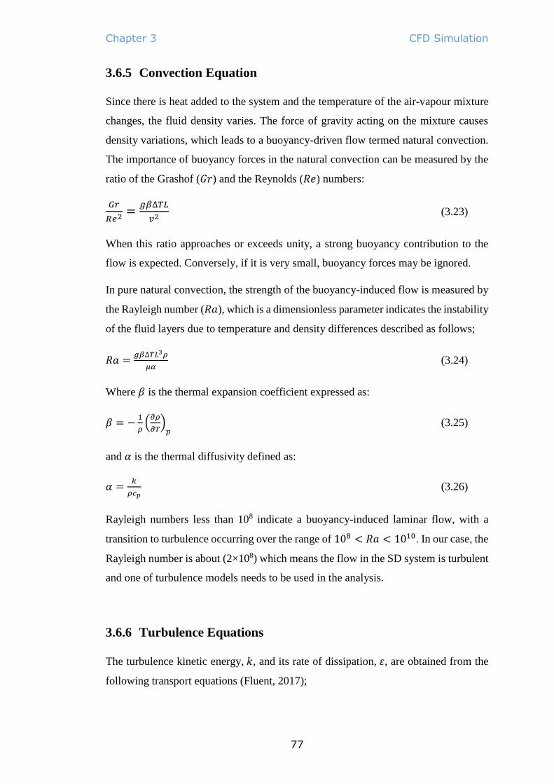
Chapter 3 CFD Simulation
77
3.6.5 Convection Equation
Since there is heat added to the system and the temperature of the air-vapour mixture
changes, the fluid density varies. The force of gravity acting on the mixture causes
density variations, which leads to a buoyancy-driven flow termed natural convection.
The importance of buoyancy forces in the natural convection can be measured by the
ratio of the Grashof (𝐺𝑟) and the Reynolds (𝑅𝑒) numbers:
𝐺𝑟
𝑅𝑒2=
𝑔𝛽∆𝑇𝐿
𝑣2 (3.23)
When this ratio approaches or exceeds unity, a strong buoyancy contribution to the
flow is expected. Conversely, if it is very small, buoyancy forces may be ignored.
In pure natural convection, the strength of the buoyancy-induced flow is measured by
the Rayleigh number (𝑅𝑎), which is a dimensionless parameter indicates the instability
of the fluid layers due to temperature and density differences described as follows;
𝑅𝑎 =𝑔𝛽∆𝑇𝐿3𝜌
𝜇𝛼 (3.24)
Where 𝛽 is the thermal expansion coefficient expressed as:
𝛽 = −1
𝜌(
𝜕𝜌
𝜕𝑇)
𝑝 (3.25)
and 𝛼 is the thermal diffusivity defined as:
𝛼 =𝑘
𝜌𝑐𝑝 (3.26)
Rayleigh numbers less than 108 indicate a buoyancy-induced laminar flow, with a
transition to turbulence occurring over the range of 108 < 𝑅𝑎 < 1010. In our case, the
Rayleigh number is about (2×10⁸) which means the flow in the SD system is turbulent
and one of turbulence models needs to be used in the analysis.
3.6.6 Turbulence Equations
The turbulence kinetic energy, 𝑘, and its rate of dissipation, 𝜀, are obtained from the
following transport equations (Fluent, 2017);

Chapter 3 CFD Simulation
78
𝜕
𝜕𝑡(𝜌𝑘) +
𝜕
𝜕𝑥𝑗(𝜌𝑘𝑢𝑗) =
𝜕
𝜕𝑥𝑗[(𝜇 +
𝜇𝑡
𝜎𝑘)
𝜕𝑘
𝜕𝑥𝑗] + Gk + 𝐺𝑏 + 𝜌𝜀 − 𝑌𝑀 + 𝑆𝑘 (3.27)
and;
𝜕
𝜕𝑡(𝜌𝜀) +
𝜕
𝜕𝑥𝑗(𝜌𝜀𝑢𝑗) =
𝜕
𝜕𝑥𝑗[(𝜇 +
𝜇𝑡
𝜎𝜀)
𝜕𝜀
𝜕𝑥𝑗] + 𝐶1ε
𝜀
𝑘(𝐺𝑘 + 𝐶3ε𝐺𝑏) − C2ερ
𝜀2
𝑘+ 𝑆𝜀
(3.28)
Two-equation turbulence models allow the determination of both, a turbulent length
and time scale by solving two separate transport equations. The (𝑘 − 𝜀) model has
become the workhorse of practical engineering flow calculations in the time since
proposed by Launder and Spalding (1972). Robustness, economy, and accuracy for a
wide range of turbulent flows explain its popularity in flow and heat transfer
simulations. This model has been extensively validated for a wide range of flows (Kim
et al, 1999).
In these equations, 𝐺𝑘 represents the generation of turbulence kinetic energy due to the
mean velocity gradients, 𝐺𝑏 is the generation of turbulence kinetic energy due to
buoyancy, 𝑌𝑀 represents the contribution of the fluctuating dilatation in compressible
turbulence to the overall dissipation rate, 𝜎𝑘 𝑎𝑛𝑑 𝜎𝜀 are the turbulent Prandtl numbers
for 𝑘 and 𝜀, respectively, and 𝑆𝑘 𝑎𝑛𝑑 𝑆𝜀 are user-defined source terms.
The turbulent or eddy viscosity 𝜇𝑡 is computed by combining 𝑘 and 𝜀 as follows:
𝜇𝑡 = 𝜌𝐶𝜇𝑘2
𝜀 (3.29)
While the model constants in equations (3.18, 19, 20) have the following default
values;
𝐶1𝜀 = 1.44, 𝐶2𝜀 = 1.92, 𝐶𝜇 = 0.09, 𝜎𝑘 = 1.0, 𝜎𝜀 = 1.3
These default values have been determined from experiments for fundamental
turbulent flows. They have been found to work fairly well for a wide range of wall-
bounded and free shear flows and they are most widely accepted (Fluent, 2017).

Chapter 3 CFD Simulation
79
3.6.7 Mass Transfer Equations
In ANSYS-Fluent, evaporation-condensation problems can be modelled using the
model of Lee (1979). The Lee model is a mechanistic model with a physical basis. It
can be used in conjunction with the VOF multiphase model. The phase-change model
proposed by Lee (1979) has been extensively used for evaporation- condensation
problem (Sun & Chen, 2014).
In the Lee model, the liquid-vapour mass transfer (evaporation-condensation) is
governed by the vapour transport equation (Fluent, 2017);
𝜕
𝜕𝑡(𝛼𝑣𝜌𝑣) + ∇ ∙ (𝛼𝑣𝜌𝑣��𝑣) = ��𝑙𝑣 − ��𝑣𝑙 (3.30)
Where
𝑣 = vapour phase
𝛼𝑣 = vapour volume fraction
𝜌𝑣 = vapour density
��𝑣 = vapour phase velocity
��𝑙𝑣, ��𝑣𝑙 = the rates of mass transfer due to evaporation and condensation,
respectively. These rates have the units of kg/s/m3
Based on the following temperature regimes, mass transfer can be described as
follows:
If 𝑇𝑙 > 𝑇𝑠𝑎𝑡 (Evaporation)
��𝑙𝑣 = 𝑐𝑜𝑒𝑓𝑓 ∗ 𝛼𝑙𝜌𝑙(𝑇𝑙−𝑇𝑠𝑎𝑡)
𝑇𝑠𝑎𝑡 (3.31)
If 𝑇𝑣 < 𝑇𝑠𝑎𝑡 (Condensation)
��𝑣𝑙 = 𝑐𝑜𝑒𝑓𝑓 ∗ 𝛼𝑣𝜌𝑣(𝑇𝑠𝑎𝑡−𝑇𝑣)
𝑇𝑠𝑎𝑡 (3.32)
Where; 𝑇𝑙 , 𝑇𝑣, 𝑇𝑠𝑎𝑡 are the liquid, vapour, and saturation temperature, respectively,
𝑐𝑜𝑒𝑓𝑓 is a coefficient that must be fine-tuned and can be derived from the
experimental results, 𝛼 and 𝜌 are the phase volume fraction and density, respectively.

Chapter 3 CFD Simulation
80
3.7 Initial and Boundary Conditions
After providing all the governing equations, the Initial and Boundary Condition have
been applied to the domain as follows;
The Initial Condition of the SD system:
The initial temperature of the system is 298 K under atmospheric pressure 101325 Pa.
The SD system has been treated as one domain and the water-liquid zone has been
adapted and patched. The water depth has been patched to the adapted region of 40
mm with a Volume Fraction 1 for the liquid phase. The solar radiation intensity and
direction have been set using solar calculator embedded in Solar Ray Tracing model
in the Fluent solver according to the geometry orientation, the location Longitude and
Altitude, and according to the day of the year, and time of the day. In this location, the
Longitude is 151.9oE and Altitude is 27.6oS.
Regarding the Boundary Conditions:
The basin base has been considered fully insulated with 0-heat flux and it participates
in the solar radiation as an opaque material with absorptivity (𝛼) = 0.8. The base
material is 3 mm thick aluminium. The cover and walls material is 3 mm thick
plexiglass. The cover and walls participate in the solar radiation as a semi-transparent
medium with transmissivity (𝜏) = 0.8. The cover and the walls have been set as mixed
thermal boundary condition including the effect of radiation and convection heat
transfer. The free stream temperature was taken as 300-310 K and the free convection
heat transfer coefficient (ℎ∞), which depends on the free stream velocity (wind
speed 𝑈∞), was taken according to the following correlation (Badran et al, 2007).
ℎ∞ = 5.7 + 3.8𝑈∞ (3.33)
Where; {0.1𝑚
𝑠≤ 𝑈∞ ≤ 5
𝑚
𝑠} within a temperature range (10 − 40 ℃)
The inlet and outlet have been set as pressure-inlet and pressure-outlet, respectively.
The inlet Volume Fraction of the liquid phase is 1 and for the outlet, this value is
calculated from neighbouring cells. For the Modified SD system, the three revolving
tubes have been set as moving walls with a rotational speed of 4.2 rad/s (40 rpm). The
revolving tubes material is PVC and they participate in the solar radiation as an opaque
material with absorptivity (𝛼) = 0.8.

Chapter 3 CFD Simulation
81
3.8 Solution Method
Using the Pressure-Based Solver (Fluent, 2017), ANSYS Fluent solves the governing
integral equations for the conservation of mass, momentum, energy, and other scalars
such as turbulence and mass transfer. A control-volume-based technique is used that
consists of:
Division of the domain into discrete control volumes using a computational
grid.
Integration of the governing equations on the individual control volumes to
construct algebraic equations for the discrete dependent variables
(“unknowns”) such as velocities, pressure, temperature, volume fraction and
conserved scalars such as energy and turbulence.
Linearization of the discretized equations and solution of the resultant linear
equations system to yield updated values of the dependent variables.
The pressure-based solver employs an algorithm which belongs to a general class of
methods called the projection method (Chorin, 1968). In the projection method the
constraint of mass conservation (the continuity equation) i.e. the velocity field, is
achieved by solving a pressure (or pressure correction) equation. The pressure equation
is derived from the continuity and momentum equations in such a way that the velocity
field, corrected by the pressure, satisfies the continuity equation.
The pressure-based solver uses a solution algorithm where the governing equations are
solved sequentially (that is, segregated from one another). Since the governing
equations are nonlinear and coupled to one another, the solution process involves
iterations wherein the entire set of governing equations is solved repeatedly until the
solution converges. The solution converges when the results have varied from the
previous iteration with only very small value defined by the user (with subsequent
iterations and all mass, momentum, energy, and scalar balances have been achieved).
The segregated algorithm is memory-efficient since the discretized equations need
only to be stored in the memory one at a time. The individual governing equations for
the variables (for example 𝑢, 𝑣, 𝑤, 𝑝, 𝑇, 𝑘, 𝜀, and so on) are solved one after another.

Chapter 3 CFD Simulation
82
Each governing equation, while being solved, is “decoupled” or “segregated” from
other equations.
With the segregated algorithm, each iteration consists of the steps illustrated in Figure
3.6 and outlined below:
1. Update fluid properties (for example, density, viscosity, specific heat)
including turbulent viscosity (diffusivity) based on the temperature obtained in
the current solution.
2. Solve the momentum equations, one after another, using the recently updated
values of pressure and face mass fluxes.
3. Solve the pressure correction equation using the recently obtained velocity
field and the mass-flux.
4. Correct face mass fluxes, pressure, and the velocity field using the pressure
correction obtained from Step 3.
5. Solve the equations for the additional scalars, such as turbulent quantities,
energy, species, and radiation intensity using the current values of the solution
variables.
6. Update the source terms arising from the interactions among different phases.
7. Check for the convergence of the equations.
In transient modelling, these steps are continued until the convergence criteria are
achieved to the current Time Step before advancing to the next Time Step.
The Timestep size, ∆t, must be small enough to resolve time-dependent features; we
need to make sure that the convergence is reached within the number of Max Iterations
per Time Step. An appropriate time step size can be estimated by:
∆𝑡 =𝑇𝑦𝑝𝑖𝑐𝑎𝑙 𝑐𝑒𝑙𝑙 𝑠𝑖𝑧𝑒
𝐶ℎ𝑎𝑟𝑎𝑐𝑡𝑒𝑟𝑖𝑠𝑡𝑖𝑐 𝑓𝑙𝑜𝑤 𝑣𝑒𝑙𝑜𝑐𝑖𝑡𝑦 (3.34)
The Time Step value is set as 0.01 second, and the Maximum number of Iterations per
Time Step is set as 1000 iterations.
In reality on the available computers, the results residuals cannot go to zero; however,
the residuals decline to some small value (round-off) and then stop changing. The
lower the residual value is, the more numerically accurate the solution. In ANSYS-
Fluent the default convergence criterion is (10-3) for all equations and (10-6) for energy
equations which are sufficient for most problems. The residual of the convergence

Chapter 3 CFD Simulation
83
criteria has been set to the following values; (10-4) for continuity, momentum,
turbulent, and volume fraction equations and (10-8) for energy and radiation equations.
The convergence has been achieved after 80 iterations for the first time step. Then it
converged after fewer iterations when advancing in time for the next time steps until
it reached 2-3 iterations after few Time Steps.
The Pressure-Implicit with Splitting Operators (PISO) Pressure-Velocity coupling
scheme has been used to improve the efficiency of the calculation and accelerate the
convergence. The PISO algorithm performs neighbour and skewness correction to
satisfy the momentum balance after solving the pressure-correction equation.
The Pressure-Based solver includes the Under-Relaxation Factor (URF) to stabilize
the iterative process and to control the update of the computed variables at each
iteration as shown in the following equation (Fluent, 2017);
∅𝑛𝑒𝑤 = ∅𝑜𝑙𝑑 + 𝑈𝑅𝐹 ∗ ∆∅ (3.35)
Where ∅ represent the value of any variable
The default values of the URF, which are between 0.1 to 1, are suitable for a wide
range of problems; however, these values can be reduced to help in achieving faster
convergence when it is necessary, especially with complex nonlinear problems. In our
case, the URF values were; for continuity equation = 0.1, for momentum equation =
0.2, for turbulent equations = 0.5, for volume fraction and mass transfer equations =
0.1, and for energy equation = 0.8.
The Double Precision solution option has been used to ensure highly accurate results
for the 3D Transient Multiphase problem under the Implicit Formulation scheme.
Figure 3.8 shows the flowchart of the solution method using the Pressure-Based solver

Chapter 3 CFD Simulation
84
Figure 3. 8 Overview of the Pressure-Based Segregated Algorithm Solution Methods
The Iterative Time Advancement (ITA) scheme

Chapter 4 Experimental Investigation
85
4 Chapter Four: Experimental Investigation
After performing the CFD simulation, the experimental tests were conducted to verify
the CFD model and to validate the results of the CFD simulation. The experimental
tests were carried out at the University of Southern Queensland campus, in
Toowoomba city (Australia) during the spring and summer seasons (from the 4th of
October 2017 to the 23rd of April 2018) and further investigations (from the 1st to the
17th of April 2019). The experimental setup, instrumentation, observation, and data
collection are described in this chapter.
4.1 Experimental Setup
Two apparatuses, the NSD system and the MSD system, were built to conduct the
experimental examinations. As described in the previous chapters, the NSD system is
a Normal Solar Still Desalination system, which has a single basin and double slope
cover. The MSD system is the Modified Solar Still Desalination system, which has the
proposed modification of three revolving tubes into its water basin. Both the NSD and
the MSD systems have the same overall dimensions, the same operation conditions,
and the same construction materials (except for the three revolving tubes). Both SD
systems were run at the same time, at the same location, and under the same weather
conditions. The designs, operating conditions, and the construction materials of both
the NSD and the MSD systems are presented in the following sections.

Chapter 4 Experimental Investigation
86
4.1.1 NSD system
The NSD system, as shown in figure 4.1, has the following design parameters;
Figure 4. 1 The schematic diagram of the NSD system design
The water basin was a rectangular shape and its dimensions were; the length = 800
mm, the width = 600 mm, and the height = 100 mm. To minimize the heat loss from
the water, the water basin was completely insulated from the outside by a 60 mm
insulation foam layer. To enhance the solar radiation absorbance and to minimize the
solar radiation reflectance, the basin liner was coated with matt black paint.
The cover was a double slope with a tilt angle of 27.6° from two opposite sides, which
is the same latitude angle of the experiment’s location. The two sides of the cover were
facing the east and the west direction.
The NSD system has a water inlet to compensate for the amount of water that
evaporates from the basin and to keep the water in the basin at a constant level. The
water level in the basin was 40 ±1 mm and was controlled by a small water-float.
To measure the productivity of the NSD system through the distillate yield, the
condensed water on the inner surface of the cover of the NSD system was collected
and discharged using two side-channels and two outlet tubes. The condensed water
was measured using a graduated flask.

Chapter 4 Experimental Investigation
87
4.1.2 MSD system
The MSD system, as shown in figure 4.2, has similar design parameters to the NSD
system except for the addition of three identical revolving tubes to the water basin of
the MSD system.
Figure 4. 2 The schematic diagram of the MSD system design
The diameter of the revolving tubes was 90 mm, the centre-to-centre distance between
the tubes was 200 mm, and the tubes centre above the base of the basin was 60 mm.
The water level in the basin was 40±1 mm, which means the tubes were semi-
immersed in the water.
Figure 4.3 shows the revolving tubes used in the MSD system. The revolving tubes
were PVC pipes plugged from both ends by push-on PVC caps with central steel
shafts. The revolving tubes were wrapped with a black absorbent mat to maximize the
solar radiation absorbance and to ensure that the outer circumference of the tubes was
always wet.

Chapter 4 Experimental Investigation
88
Figure 4. 3 The three revolving tubes used in the MSD system
Figure 4.4 shows three worm gear DC motors connected to three revolving tubes of
the MSD system and run by a variable DC power supply. The DC motors’
specifications were; maximum voltage = 16 V, maximum power = 50 W, maximum
torque = 5 N∙m, and maximum rotation speed = 65 rpm. To control the rotational speed
of the revolving tubes, these motors were powered by a variable (switch-mode Lab)
DC power supply (0-16V/ 25A).
Figure 4. 4 a) The DC motor b) The coupling arrangement to the MSD system, c) The variable DC power supply
that used in the experiment

Chapter 4 Experimental Investigation
89
4.2 Construction Materials
In both the NSD and the MSD systems, the basin was made of a 3 mm thick aluminium
sheet, the cover was made of a 3 mm thick clear plexiglass sheet, and the insulation
was made of a 60 mm thick XPS foam board. In the MSD system, the tubes were made
of a 90 mm diameter PVC pipe. The construction materials were chosen according to
their good thermal and optical properties. According to the literature review, the
aluminium basins were preferable due to their good physical and thermal properties
(Malaiyappan & Elumalai, 2016). Aluminium is lightweight, anti-corrosion, and the
coated aluminium has a good absorbance to solar radiation. The plexiglass has many
advantages over the glass, it has a lighter weight, is unbreakable, easy to fabricate,
safer, has a higher transmittance to solar radiation, and is much cheaper than glass.
The PVC tube is widely abundant at trivial cost and it is very lightweight, which means
it requires less energy for rotating by a small DC motor. The XPS foam has good
insulation properties and it is weather and rain resistant. All materials used are
available in local markets at moderate prices. Table 4.1 lists the Thermal and Optical
properties of the selected construction materials. Figure 4.5 shows the constructed
NSD and MSD systems used in this work.
Table 4. 1 The thermal and optical properties of the construction materials used in this project
Properties Aluminium Plexiglass PVC XPS foam
Density 𝜌 (𝑘𝑔 𝑚3⁄ ) 2790 1190 1470 20
Specific Heat 𝑐𝑝 (𝐽 𝑘𝑔 ∙ 𝐾)⁄ 880 1450 850
Thermal Conductivity 𝑘 (𝑊 𝑚 ∙ 𝐾)⁄ 168 0.7 0.2 0.02
Absorbance 0.88 (coated) 0.05 0.88 (coated)
Transmittance 0 0.90 0
Reflectance 0.12 0.05 0.12

Chapter 4 Experimental Investigation
90
Figure 4. 5 The experimental apparatus, the NSD system (left) and the MSD system (right) the MSD was without water to show the inside

Chapter 4 Experimental Investigation
91
4.3 Instrumentation
Some instrumentation were used in the experiment part of this study to measure the
temperatures, the output distillate water, and the weather conditions.
A calibrated thermometer Data-logger with twelve K-type thermocouples were used
to measure the temperature of the water, the temperature of the vapour, the temperature
of the cover, and the temperature of the basin in both the NSD and the MSD systems.
The type of Datalogger was (Lutron BTM-4208SD) 12 Channels Thermometer
recorder with a capability to store the data of many days as spreadsheets on an external
memory card.
Two graduated measuring cylinders (500 ±5 ml) and (50 ± 0.5 ml) were used to
measure the volume of the distillate yield or the productivity of each SD system. An
electronic scale (0 to 5000 ±0.5 g) also was used to measure the mass of the output
water.
The meteorological parameters (i.e. the weather conditions) such as the solar intensity,
the wind speed, and the relative humidity were obtained from the official weather
station of the University of Southern Queensland (2019). The weather station is
reliable and very close to the experiment location. The data from the weather stations
of the Toowoomba city that run by the Australian Government- Bureau of
Meteorology (2019) also were considered reliable and were used for confirming the
readings. Figure 4.6 shows the instruments used in this study and Table 4.2 lists their
technical specifications as provided by the manufacturers.

Chapter 4 Experimental Investigation
92
Figure 4. 6 a) the thermocouples and the data logger b) the measuring cylinders and electronic scale
Table 4. 2 The technical specifications of the instruments used in the experimental tests
Instrument Resolution Range Accuracy Error %
Temperature Logger 0.1°C -50 to 999.9°C ±0.5°C ±0.4%
K-type thermocouples -40 to 260°C ±0.5°C ±0.4%
Measuring cylinder1 5 ml 50 to 500 ml ±5 ml ±1%
Measuring cylinder2 1 ml 5 to 50 ml ±0.5 ml ±1%
Electronic scale 1 g 0 to 5000 g ±0.5 g ±0.1%
Electronic stopwatch 0.01 s 0 to 5999 s ±0.1 s ±0.001%
a
) b)

Chapter 4 Experimental Investigation
93
4.4 Observation
The experimental tests were carried out at the University of Southern Queensland
campus, in Toowoomba, Australia during the spring and summer seasons due to the
higher levels of solar exposure in these two seasons when compared to other seasons.
According to the Australian Government Bureau of Meteorology (2019), in
Toowoomba city, the average daily solar exposure for the period of six months from
October to April is about (21 to 24 MJ/m2) while it is about (12 to 15 MJ/m2) from
May to September. Therefore, the experimental tests were run from the 4th of October
2017 to the 23rd of April 2018 and further investigations were undertaken from the 1st
to the 17th of April 2019.
Figure 4.7 shows the average daily solar exposure in Australia during the spring and
summer seasons from October to April, and Figure 4.8 during the autumn and winter
seasons from May to September (Bureau of Meteorology, 2019).
Figure 4. 7 The average daily solar exposure in Australia during the spring and summer seasons (Bureau of
Meteorology, 2019). (CC licenced Product Code: IDCJCM0019). The star symbol is added to the original picture
to indicate the location of Toowoomba city where the experiment was performed

Chapter 4 Experimental Investigation
94
Figure 4. 8 The average daily solar exposure in Australia during the autumn and winter seasons (Bureau of
Meteorology, 2019). (CC licenced Product Code: IDCJCM0019). The star symbol is added to the original picture
to indicate the location of Toowoomba city where the experiment was performed
The geographical location of the experimental investigations was, Longitude =
151.931º East, Latitude = 27.601º South, and Elevation = 691 m. The orientation of
the apparatuses (Both SD systems) was due north because the site was in the southern
hemisphere. The two sides of the SD system cover were facing the east and the west.
Figure 4.9 shows the satellite image of the experiment geographical location taken by
Google Maps (2019) and figure 4.10 shows the SD systems orientation during the
experimental tests.
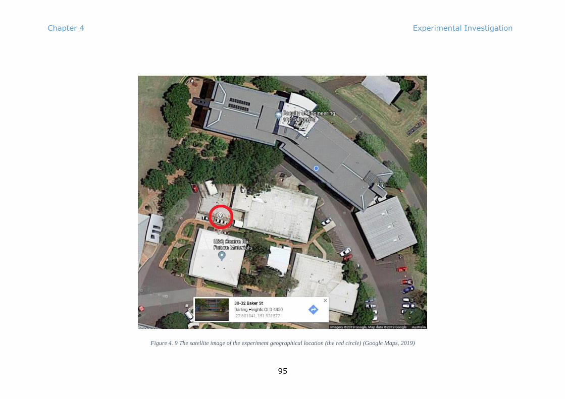
Chapter 4 Experimental Investigation
95
Figure 4. 9 The satellite image of the experiment geographical location (the red circle) (Google Maps, 2019)

Chapter 4 Experimental Investigation
96
Figure 4. 10 The two SD system during the experiment and the orientation

Chapter 4 Experimental Investigation
97
To evaluate and compare the performance of the MSD system and the NSD system,
both SD systems were run at the same time, at the same location, and under the same
weather conditions. Several parameters were measured during the experimental
investigations and the observation methodology was as follows;
1. The thermometer data-logger with twelve channels was set to record the
temperature of the water, the temperature of the vapour, the temperature of the
basin, and the temperature of the cover for both the SD systems every five
minutes and stored the data into spreadsheets on an external memory card. The
data was continually transferred to the computer.
2. Twelve K-type thermocouples were connected to the data-logger and
distributed between the two SD systems as follows; four thermocouples placed
into the water, four thermocouples placed into space above the water, two
thermocouples attached to the basins, and two thermocouples attached to the
covers.
3. The weather conditions such as the ambient temperature, the solar intensity,
the wind speed, and the relative humidity were collected from the nearby
weather station of the University of Southern Queensland and the weather
stations of Toowoomba city.
4. The distillate water or the productivity of the NSD system and the MSD system
were collected into two separate water containers. The collected water was
measured daily in the early morning to find out the daily productivity of each
SD system. A digital scale and measuring cylinders were used for measuring
the daily productivity of both the SD systems.
5. The hourly yield of both the SD systems was measured on selected clear days
about the middle of every month during the experimental period.
Figure 4.11 shows a schematic diagram of the experiment layout and indicates the
locations of the thermocouples.

Chapter 4 Experimental Investigation
98
Figure 4. 11 The experiment layout and the locations of the thermocouples

Chapter 4 Experimental Investigation
99
4.5 Data Collection
The experimental data were recorded in three of datasheets as follows;
1. The first data sheet was used to record the following parameters every 5
minutes 24 hours a day, 7 days a week during the whole period of the
experimental investigations. The data captured included the temperature of the
water, the temperature of the vapour, the temperature of the basin, and the
temperature of the cover of both the MSD system and the NSD system. The
data also included the weather conditions, the ambient temperature, the solar
intensity, the wind speed, and the relative humidity. Table 4.3 shows the first
data sheet used in in the experimental part of this study.
2. The second data sheet was used to record the daily productivity (or the daily
distillate yield) of both the SD systems. The data collection also included; the
daily insolation (or the daily solar exposure), the maximum ambient
temperature, the average wind speed, the average relative humidity, and the
average cloud cover amount. The daily maximum temperature of the water, the
vapour, the cover, and the basin of both the SD systems were recorded as well.
The daily efficiency of both the SD systems and the enhancement in the daily
efficiency and the daily productivity due to the modification were calculated
and recorded daily in the same datasheet. Table 4.4 shows the second data sheet
used in the experimental part of this study.
3. The third data sheet was used to record the hourly productivity and the hourly
insolation of the selected days during the experimental tests. It also used to
record the hourly efficiency and the enhancement in the hourly productivity
and hourly efficiency. Table 4.5 shows the third data sheet used in the
experimental part of this study.

Chapter 4 Experimental Investigation
100
Table 4. 3 The first datasheet of the experimental data collection
Time Water
Temperature
(°C)
Vapour
Temperature
(°C)
Basin
Temperature
(°C)
Cover
Temperature
(°C)
Ambient
Temperature
(°C)
Wind speed
(km/hr)
Relative
Humidity
(%)
Solar intensity
(W/m2)
MSD NSD MSD NSD MSD NSD MSD NSD
06:00
06:05
Table 4. 4 The second datasheet of the experimental data collection
Day Daily
Solar
Exposure
= Daily
Insolation
(MJ/m2)
Daily
Max.
Ambient
Temperat
ure
(°C)
Daily
Ave.
Wind
Speed
(km/hr)
Daily
Ave.
Relative
Humidity
(%)
Daily
Ave.
Cloud
Amount
(Oktas)
Daily Max.
Water
Temperature
(°C)
Daily Max.
Vapour
Temperature
(°C)
Daily Max.
Basin
Temperature
(°C)
Daily Max.
Cover
Temperature
(°C)
Daily
Productivity
(kg/m2.day)
Daily
Thermal
Efficiency
(%)
Daily
Productivity
Enhancement
(%)
Daily
Efficiency
Enhancement
(%)
MSD NSD MSD NSD MSD NSD MSD NSD MSD NSD MSD NSD
Table 4. 5 the third datasheet of the experimental data collection
Day/Time Hourly insolation
(MJ/m^2)
Hourly Productivity
(ml/hr)
Hourly efficiency
(%)
Enhancement in hourly
productivity
(%)
Enhancement in hourly
efficiency
(%) MSD NSD MSD NSD

Chapter 5 Results and Discussions
101
5 Chapter Five: Results and Discussions
This chapter presents and discusses the results of the CFD simulation and the results
of the experimental investigation that were described in Chapters Three and Four,
respectively. This chapter is divided into the following sections; the results of the CFD
simulation, the results of the experimental investigation, and the CFD model
validation.
5.1 Results of the CFD Simulation
Using the CFD Fluent solver which is part of ANSYS 19.1 software, the CFD
simulation was carried out to simulate both the MSD and the NSD systems. As
described in Chapter Three, the simulation was conducted as three-dimensional,
transient, and multiphase (with phase change) analysis. The solution method was an
iterative implicit scheme in double precision, using pressure-based solver. For the
phase change (evaporation-condensation), the Lee model included in the VOF
multiphase model was applied. For the turbulence flow, the 𝑘 − 𝜖 turbulence model
was used. For the solar radiation load, the solar ray-tracing model was applied.
As mentioned also in Chapter Three, mixed convection and radiation boundary
conditions were applied to the walls; including the cover in both the SD systems and
the revolving tubes in the MSD system. The basin wall was considered fully insulated
with no heat losses. All walls participated in the solar radiation; the cover was
transparent, and the basin and the revolving tubes were opaque objects. There were
two pressure outlets and one velocity inlet in every SD system. The numerical model
dimensions were as the experimental model dimensions; the basin was 800 𝑚𝑚 ×
600 𝑚𝑚 × 100 𝑚𝑚, the cover slope angle was 27.5°, the water depth was 40 𝑚𝑚,
the revolving tubes’ diameter was 90 𝑚𝑚, the tubes centre-to-centre was 200 𝑚𝑚 and
the tube centre to the basin was 60 𝑚𝑚. The results obtained from the CFD simulation
are presented in the following sections.

Chapter 5 Results and Discussions
102
5.1.1 Solar Radiation
Figure 5.1 shows the rate of the absorbed solar radiation (solar heat flux) into the
absorber of the MSD and NSD systems. The results show that in addition to the solar
radiation absorbed by the base in both the SD systems, the MSD system has the
advantage of absorbing solar radiation by the revolving tubes. According to the results,
the MSD system absorbs more solar energy than the NSD system. As solar radiation
is the only input heat source, solar radiation is the most important factor that affects
the performance of the SD systems. Increasing the amount of absorbed solar radiation
by the SD system means an SD system with higher productivity and higher thermal
efficiency.
Figure 5. 1 The solar radiation distribution of the MSD system (left) and the NSD system (right)
Orthogonal solar radiation = 1000 W/m2, ambient temperature = 300 K, wind Speed = 5 m/s, atmospheric
pressure = 1 bar, tube’s rotation speed = 40 rpm, water depth = 40 mm, tube’s diameter = 90 mm

Chapter 5 Results and Discussions
103
5.1.2 Temperature
Figures 5.2 and 5.3 show the temperature distribution in the mid plane of the MSD
system and the NSD system at two different time steps. The results showed that the
temperature of the MSD system was a little higher than the NSD system. The
explanation to this case is the revolving tubes of the MSD system was heated by the
solar radiation. The rotational movement of these tubes raise the temperature of the
water in the basin and heats up the surrounding vapour. According to the results, there
was about 5ºC difference between the temperature of the MSD system and the
temperature of the NSD system. Increasing the absorbance of solar radiation in the
MSD system was the reason for increasing the difference in the temperature between
the two SD systems. Temperature is a very important factor for the SD systems’
performance. Higher water temperature means more evaporation and hotter air carries
more moisture, which leads to an increase in the productivity of the SD system.
Figure 5. 2 The temperature distribution in the midplane of the MSD system (left) and the NSD system (right)
after one hour. Orthogonal solar radiation = 1000 W/m2, ambient temperature = 300 K, wind Speed = 5 m/s,
atmospheric pressure = 1 bar, tube’s rotation speed = 40 rpm, water depth = 40 mm, tube’s diameter = 90 mm

Chapter 5 Results and Discussions
104
Figure 5. 3 The temperature distribution in the midplane of the MSD system (upper) and the NSD system (lower)
after two hours. Orthogonal solar radiation = 1000 W/m2, ambient temperature = 300 K, wind Speed = 5 m/s,
atmospheric pressure = 1 bar, tube’s rotation speed = 40 rpm, water depth = 40 mm, tube’s diameter = 90 mm

Chapter 5 Results and Discussions
105
5.1.3 Pressure
Figure 5.4 shows the contours of the static gauge pressure of a central cross-section of
both the MSD and the NSD systems after one hour. The results showed that the
modification of the revolving tubes that was introduced to the MSD system did not
affect the pressure distribution of the SD system. The explanation to this case is, the
temperature was rising slowly, and there were two pressure outlets. The outlet pressure
keeps the pressure in balance with the surrounding atmosphere.
Figure 5. 4 The pressure contours of the central cross-section of the MSD system (left) and the NSD system
(right). Orthogonal solar radiation = 1000 W/m2, ambient temperature = 300 K, wind Speed = 5 m/s,
atmospheric pressure = 1 bar, tube’s rotation speed = 40 rpm, water depth = 40 mm, tube’s diameter = 90 mm

Chapter 5 Results and Discussions
106
5.1.4 Density
Figure 5.5 shows the density contours of a central cross-section of both the MSD and
the NSD systems. The results showed that the density distribution within the MSD
system is closely similar to that of the NSD system except for a thin layer of water
density around the circumferences of the revolving tubes in the MSD system. There
were three main distinctive zones; the upper zone which is occupied by the vapour
with density of about (0.7 kg/m3), the lower zone which is occupied by water with
density of about (998 kg/m3), and the in-between zone (layer), which is a mixture
between the vapour and the water. According to the results, the MSD system has the
advantage of increasing the surface area of the evaporation, which leads to an increase
in the evaporation rate.
Figure 5. 5 The density contours of the central cross-section of the MSD system (left) and the NSD system (right)
Orthogonal solar radiation = 1000 W/m2, ambient temperature = 300 K, wind Speed = 5 m/s, atmospheric
pressure = 1 bar, tube’s rotation speed = 40 rpm, water depth = 40 mm, tube’s diameter = 90 mm

Chapter 5 Results and Discussions
107
5.1.5 Velocity
Figure 5.6 shows the velocity contours of a central cross-section of both the MSD and
the NSD systems. The results showed that the MSD system has a higher vapour
velocity than the NSD system. The explanation to this case is that the flow inside the
cavity of the MSD system was more turbulence than the NSD system due to the
modification of the revolving tubes. According to the results, the vapour velocity
ranged from (0 m/s) to about (0.3 m/s).
Figure 5. 6 The velocity contours of the central cross-section of the MSD system (left) and the NSD system (right)
Orthogonal solar radiation = 1000 W/m2, ambient temperature = 300 K, wind Speed = 5 m/s, atmospheric
pressure = 1 bar, tube’s rotation speed = 40 rpm, water depth = 40 mm, tube’s diameter = 90 mm

Chapter 5 Results and Discussions
108
5.1.6 Evaporation and Condensation
Figure 5.7 shows the evaporation rate of the MSD and the NSD systems after one hour.
Figure 5.8 (a) and (b) show the progressive condensation film mass of the MSD system
and the NSD system at two different times. The results show that the MSD system has
higher evaporation and higher condensation rates than the NSD system. According to
the results, the evaporation and condensation rates of the MSD system were about
double that of the NSD system. The explanation to this results is, the water temperature
of the MSD system was higher than the water temperature of the NSD system (as
presented in section 5.1.2, figures 5.2 & 5.3), which means faster evaporation. Since
temperature is a big factor on the amount of the water particles that evaporate, causes
them to move upward far from the water surface towards the cover of the SD system.
Another reason is, the surface area of the evaporation in the MSD system was greater
than that in the NSD system, which also leads to an increase in the evaporation rate.
The increase in the evaporation enhances the possibility of an increase in the
condensation hence increase the productivity of the SD system.
Figure 5. 7 The evaporation rate in the middle plane of the MSD system (left) and the NSD system (right) after 1
hour. Orthogonal solar radiation = 1000 W/m2, ambient temperature = 300 K, wind Speed = 5 m/s, atmospheric
pressure = 1 bar, tube’s rotation speed = 40 rpm, water depth = 40 mm, tube’s diameter = 90 mm

Chapter 5 Results and Discussions
109
Figure 5.8 (a) The condensation film mass of the MSD system (left) and the NSD system (right) after 30 minutes
Orthogonal solar radiation = 1000 W/m2, ambient temperature = 300 K, wind Speed = 5 m/s, atmospheric
pressure = 1 bar, tube’s rotation speed = 40 rpm, water depth = 40 mm, tube’s diameter = 90 mm
Figure 5. 8 (b) The condensation film mass of the MSD system (left) and the NSD system (right) after 1 hour
Orthogonal solar radiation = 1000 W/m2, ambient temperature = 300 K, wind Speed = 5 m/s, atmospheric
pressure = 1 bar, tube’s rotation speed = 40 rpm, water depth = 40 mm, tube’s diameter = 90 mm

Chapter 5 Results and Discussions
110
5.2 Results of the Experimental Investigation
After conducting the experimental investigations (from the 4th of October 2017 to the
23rd of April 2018) and further investigations (from the 1st to the 17th of April 2019) to
both the MSD and the NSD systems in the University of Southern Queensland-
Toowoomba city- Australia, the following results were obtained.
5.2.1 Temperature Profile
The experimental data showed the following results;
1- In both the SD systems, the temperature starts rising at about 7:00 am, peaks
at about 2:00 pm, and then starts declining slowly up to the next day morning.
2- In both the SD systems, the water temperature has the highest value during the
peak time from about 2:00 pm to approximately 3:00 pm.
3- In both the SD systems, the vapour temperature could be a little higher than the
water temperature before noon, then becomes nearly equal to the water
temperature at noon, and then lower than the water temperature afternoon.
4- In both the SD systems, the basin temperature was nearly equal to the water
temperature except for the noon period when the water temperature was a little
higher than the basin temperature.
5- In both the SD systems, during the peak time, the highest temperature was the
temperature of the water and vapour followed by the temperature of the basin
and then the temperature of the cover.
6- In both the SD systems, the cover temperature had the lowest temperature
values, and it could be lower than the ambient temperature during the night and
up to the early morning of the next day.
7- The temperature of the MSD system was always higher than the temperature
of the NSD system, especially during the noon period or the peak time.
8- During the peak time, the temperature of the MSD system was higher than the
temperature of the NSD system by an average of 5℃ for the temperature of the
water, vapour, and the basin, and by an average of 3℃ for the temperature of
the cover.

Chapter 5 Results and Discussions
111
9- During the peak time, the average temperature difference between the water
and the cover was about 15℃ in the MSD system and about 12℃ in the NSD
system.
Table 5.1 lists the average temperature values during the noon and the maximum-
recorded temperature in both SD systems.
Table 5. 1 The temperature of the MSD system and the NSD system (the average value is from the maximum
temperature of all days, and the maximum value is the maximum recorded during the whole period of the
experiment)
Average Temperature (℃) Maximum Temperature (℃)
MSD NSD MSD NSD
Water temperature 55.7 50.5 73.9 68.6
Vapour temperature 54.6 49.5 74.2 69.3
Basin temperature 53.4 48.1 70.1 65.4
Cover temperature 41.9 38.9 57.7 55.1
Figure 5.10 shows the temperature profile of the water, the vapour, the cover, the basin,
and the ambient temperature of both the MSD and the NSD systems over a period from
6:00 am of the 4th of April 2019 to 7:00 am of the next day the 5th of April 2019.
The temperature profile of selected days, during the experiment period, is presented in
Appendix A.

Chapter 5 Results and Discussions
112
Figure 5. 9 The temperature profile of the components of the MSD system and the NSD system
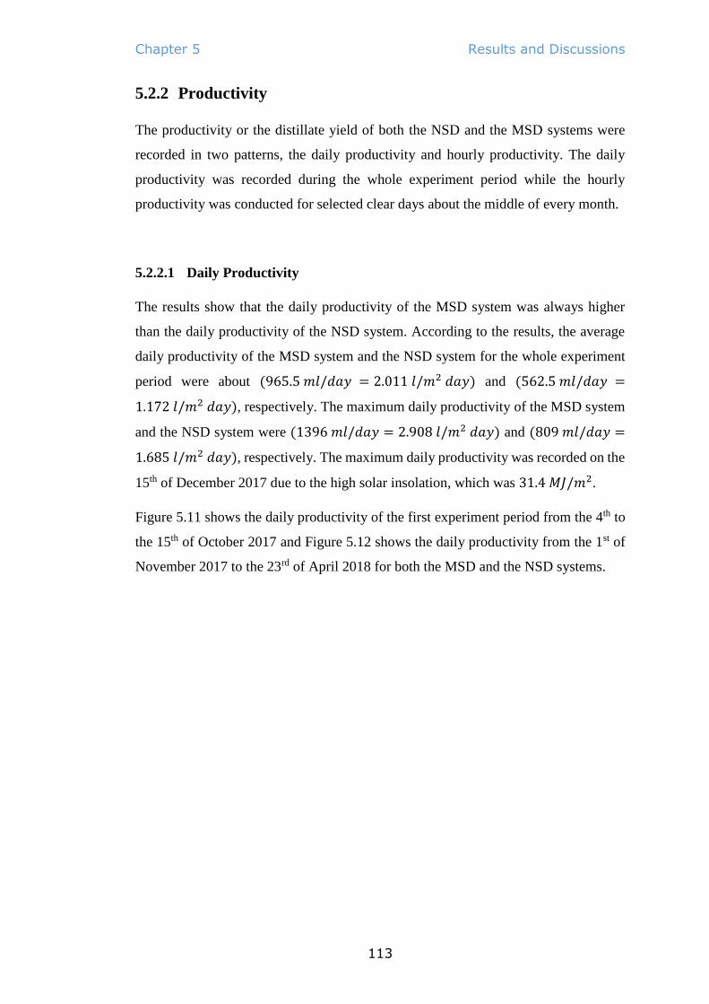
Chapter 5 Results and Discussions
113
5.2.2 Productivity
The productivity or the distillate yield of both the NSD and the MSD systems were
recorded in two patterns, the daily productivity and hourly productivity. The daily
productivity was recorded during the whole experiment period while the hourly
productivity was conducted for selected clear days about the middle of every month.
5.2.2.1 Daily Productivity
The results show that the daily productivity of the MSD system was always higher
than the daily productivity of the NSD system. According to the results, the average
daily productivity of the MSD system and the NSD system for the whole experiment
period were about (965.5 𝑚𝑙/𝑑𝑎𝑦 = 2.011 𝑙/𝑚2 𝑑𝑎𝑦) and (562.5 𝑚𝑙/𝑑𝑎𝑦 =
1.172 𝑙/𝑚2 𝑑𝑎𝑦), respectively. The maximum daily productivity of the MSD system
and the NSD system were (1396 𝑚𝑙/𝑑𝑎𝑦 = 2.908 𝑙/𝑚2 𝑑𝑎𝑦) and (809 𝑚𝑙/𝑑𝑎𝑦 =
1.685 𝑙/𝑚2 𝑑𝑎𝑦), respectively. The maximum daily productivity was recorded on the
15th of December 2017 due to the high solar insolation, which was 31.4 𝑀𝐽/𝑚2.
Figure 5.11 shows the daily productivity of the first experiment period from the 4th to
the 15th of October 2017 and Figure 5.12 shows the daily productivity from the 1st of
November 2017 to the 23rd of April 2018 for both the MSD and the NSD systems.

Chapter 5 Results and Discussions
114
Figure 5. 10 The daily productivity of the MSD system and the NSD system during October 2017

Chapter 5 Results and Discussions
115
Figure 5. 11 The daily productivity of the MSD system and the NSD system from the 1st of November 2017 to the 23rd of April 2018

Chapter 5 Results and Discussions
116
5.2.2.2 Hourly Productivity
The results show that the hourly productivity of the MSD system was always higher
than the productivity of the NSD system. The hourly data collection was conducted
for selected clear days around the middle of every month during the experimental
period. The hourly productivity was measured every hour from 9:00 am to 5:00 pm.
According to the results, the maximum hourly productivity was during noon or the
peak time about 2:00 pm. The selected days are; the 13th of October 2017, the 15th of
November 2017, the 14th of December 2017, the16th of January 2018, the 14th of
February 2018, the16th of March 2018, and the 16th of April 2018.
Figures 5.13 and 5.14 show the hourly productivity and the cumulative hourly
productivity on the 13th of October 2017 of both the MSD and the NSD systems.
The hourly productivity and the cumulative hourly productivity of selected days are
presented in Appendix A.

Chapter 5 Results and Discussions
117
Figure 5. 12 The hourly productivity the MSD and the NSD systems on the 13th of October 2017
The daily insolation 24.7 MJ/m2, Max. Ambient temperature 27.5 ºC, Mean wind speed 16 km/hr, average relative humidity 56%

Chapter 5 Results and Discussions
118
Figure 5. 13 The cumulative hourly productivity the MSD and the NSD systems on the 13th of October 2017
The daily insolation 24.7 MJ/m2, Max. Ambient temperature 27.5 ºC, Mean wind speed 16 km/hr, average relative humidity 56%

Chapter 5 Results and Discussions
119
5.2.3 Efficiency
The daily and the hourly efficiency for both the SD systems were estimated as follows;
5.2.3.1 Daily efficiency
The daily efficiency 𝜂 can be found from equations 3.2 and 3.3 in Chapter Three, or
as follows;
𝜂% =𝑇ℎ𝑒 ℎ𝑒𝑎𝑡 𝑢𝑠𝑒𝑑 𝑖𝑛 𝑡ℎ𝑒 𝑒𝑣𝑎𝑝𝑜𝑟𝑎𝑡𝑖𝑜𝑛 (𝑜𝑢𝑡𝑝𝑢𝑡)
𝑇ℎ𝑒 𝑡𝑜𝑡𝑎𝑙 𝑠𝑢𝑝𝑝𝑙𝑖𝑒𝑑 ℎ𝑒𝑎𝑡 (𝑖𝑛𝑝𝑢𝑡)× 100% (5.1)
From the above equation, the efficiency of the NSD system 𝜂𝑁𝑆𝐷 will be;
𝜂𝑁𝑆𝐷% =��𝑒×𝐿𝑣
𝐺𝑠×𝐴𝑠× 100% (5.2)
While the efficiency of the MSD system 𝜂𝑀𝑆𝐷 will be;
𝜂𝑀𝑆𝐷% =��𝑒×𝐿𝑣
(𝐺𝑠×𝐴𝑠)+𝐸𝑚× 100% (5.3)
Where; ��𝑒 is the daily distillate yield or daily productivity, 𝐿𝑣 is the latent heat of
vaporisation, 𝐺𝑠 is the daily solar exposure or the daily insolation, 𝐴𝑠 is the surface
area of the SD system, and 𝐸𝑚 is the electric energy used to run the revolving tubes in
the MSD system.
𝐸𝑚 = 𝑉 × 𝐴 × 𝑛𝑢𝑚𝑏𝑒𝑟 𝑜𝑓 ℎ𝑜𝑢𝑟𝑠 × 3600 (5.4)
Where; 𝑉 𝑎𝑛𝑑 𝐴 are the voltage and the current that required to run three motors and
were recorded from the power supply. (𝑉 = 10 𝑉 , 𝑎𝑛𝑑 𝐴 = 5 𝐴).
The results showed that the daily efficiency of the MSD system was always higher
than the daily efficiency of the NSD system. According to the results, the average daily
efficiency was 18.77% and 12.11% for the MSD system and the NSD system,
respectively. The maximum daily efficiency was 21.01% and 13.12% for the MSD
system and the NSD system, respectively.
Figure 5.15 shows the daily efficiency for the period from the 4th to the 15th of October
2017 and Figure 5.16 shows the daily efficiency from the 1st of November 2017 to the
23rd of April 2018 for both systems.

Chapter 5 Results and Discussions
120
Figure 5. 14 The daily efficiency of the MSD system and the NSD system during October 2017

Chapter 5 Results and Discussions
121
Figure 5. 15 The daily efficiency of the MSD system and the NSD system from the 1st of November 2017 to the 23rd of April 2018

Chapter 5 Results and Discussions
122
5.2.3.2 Hourly efficiency
The same equations used in calculating the daily efficiency were used to calculate the
hourly efficiency using the values of the hourly productivity and the hourly insolation.
Similar to the hourly productivity the hourly efficiency was estimated to every hour
from 10:00 am to 5:00 pm for the same selected days to conduct the hourly
productivity as presented in section 5.2.2.2.
The results showed that the hourly efficiency of the MSD system was always higher
than the hourly efficiency of the NSD system. According to the results, the average
hourly efficiency for the conducted hours was 24.8% and 15.5% for the MSD system
and the NSD system, respectively. The maximum hourly efficiency was recorded
during the peak time about 2:00 pm on the 15th of November 2017 and it was 37.4%
and 23.9% for the MSD system and the NSD system, respectively.
Figure 5.17 shows the hourly efficiency on the 13th of October 2017.
The hourly efficiency of selected days are presented in Appendix A. Table of the
hourly insolation, hourly productivity, hourly efficiency, and the enhancement in the
hourly productivity and hourly efficiency is presented in Appendix B.

Chapter 5 Results and Discussions
123
Figure 5. 16 The hourly efficiency of the MSD system and the NSD system on the 13th of October 2017

Chapter 5 Results and Discussions
124
5.2.4 Enhancement in Productivity and Efficiency
The enhancement in daily productivity and the daily efficiency was found from the
following relations;
𝑃𝑟𝑜𝑑𝑢𝑐𝑡𝑖𝑣𝑖𝑡𝑦 𝐸𝑛ℎ𝑎𝑛𝑐𝑒𝑚𝑒𝑛𝑡% =𝑀𝑆𝐷 𝑝𝑟𝑜𝑑𝑢𝑐𝑡𝑖𝑣𝑖𝑡𝑦−𝑁𝑆𝐷 𝑝𝑟𝑜𝑑𝑢𝑐𝑡𝑖𝑣𝑖𝑡𝑦
𝑁𝑆𝐷 𝑝𝑟𝑜𝑑𝑢𝑐𝑡𝑖𝑣𝑖𝑡𝑦× 100%
(5.5)
𝐸𝑓𝑓𝑖𝑐𝑖𝑒𝑛𝑐𝑦 𝐸𝑛ℎ𝑎𝑛𝑐𝑒𝑚𝑒𝑛𝑡% =𝑀𝑆𝐷 𝑒𝑓𝑓𝑖𝑐𝑖𝑒𝑛𝑐𝑦−𝑁𝑆𝐷 𝑒𝑓𝑓𝑖𝑐𝑖𝑒𝑛𝑐𝑦
𝑁𝑆𝐷 𝑒𝑓𝑓𝑖𝑐𝑖𝑒𝑛𝑐𝑦× 100%
(5.6)
According to the results, the average enhancement in daily productivity and daily
efficiency was approximately 70.7% and 54.3%, respectively. The maximum
enhancement in the daily productivity and the daily efficiency were about 74.8% and
63.4%, respectively.
Figure 5.18 shows the enhancement in the daily productivity and the daily efficiency
of the MSD system with respect to NSD system for the period from the 4th to the 15th
of October 2017. Figure 5.19 shows the enhancement in the daily productivity and the
daily efficiency of the MSD system with respect to NSD system for the period from
the 1st of November 2017 to the 23rd of April 2018.

Chapter 5 Results and Discussions
125
Figure 5. 17 The enhancement in the daily productivity and the daily efficiency of the MSD system respect to NSD system during October 2017

Chapter 5 Results and Discussions
126
Figure 5. 18 The enhancement in the daily productivity and the daily efficiency of the MSD system respect to NSD system from the 1st of November 2017 to the 23rd of April 2018

Chapter 5 Results and Discussions
127
5.2.5 Datasheets
As presented in Chapter Four, the data collection was recorded into three types of
datasheets. The data from these data sheets were used in the previous sections to
present the temperature profile, the hourly and daily productivity, the hourly and daily
efficiency, and the enhancement in the daily productivity and efficiency.
Table 5.1 and Table 5.2 show a sample of the first and the second datasheets,
respectively. The first datasheets of some selected days, the second datasheets of all
days, and the third data sheet of all selected days are presented in Appendix B.

Chapter 5 Results and Discussions
128
Table 5. 2 The first pattern of datasheets- the data of the 4th of April 2019 (the temperature used in figure 5.10)
Time Water
Temperature
(ºC)
Vapour
Temperature
(ºC)
Basin
Temperature
(ºC)
Cover
Temperature
(ºC)
Ambient
Temperature
(ºC)
Wind speed
(km/hr)
Relative
Humidity
(%)
Solar intensity
(W/m2)
MSD NSD MSD NSD MSD NSD MSD NSD
10:00:00 31.3 30.2 38.4 37.2 31.4 31.1 26.4 26.7 19 2 67 703
10:10:00 32.6 31.4 39.9 38.1 32.9 32.3 27.2 27.4 19.1 21 65 722
10:20:00 34.1 32.6 40 38.5 34.3 33.5 27.5 27.6 19.4 23 64 742
10:30:00 35.5 33.9 41.1 39.7 35.5 34.6 28.5 28.7 19.8 2 64 759
10:40:00 36.9 35 41.9 40.3 37.1 35.8 28.9 28.9 20.1 27 58 775
10:50:00 38.3 36.2 42.7 41.5 38.4 36.9 30.4 30.4 20.3 23 56 789
11:00:00 39.6 37.4 44.1 42.8 39.7 38.1 31 30.8 20.4 31 57 798
11:10:00 41 38.5 44.6 44.1 40.9 39.4 31.8 31.7 20.6 18 58 809
11:20:00 42.3 39.6 46.1 44.5 42.1 40.3 32.4 32.2 21.1 11 56 819
11:30:00 43.5 40.8 46.6 46.2 43.4 41.5 33.7 33.2 21.2 6 57 826
11:40:00 44.7 41.8 48 46.6 44.6 42.6 34.4 33.2 21.7 27 54 831
11:50:00 46 42.7 48 47 45.7 43.5 34.7 33.8 21.2 24 57 828
12:00:00 47.1 43.6 49.9 48 46.6 44.3 36 34.3 21.3 19 55 833
12:10:00 48.2 44.4 50.4 48.8 47.6 45.1 36.5 35.2 21.1 26 57 830
12:20:00 49.4 45.1 50.9 47.9 48.4 45.6 36.6 35.2 21.3 13 56 830
12:30:00 50.2 45.7 52.4 48.8 49.5 46.3 38 36 21.2 5 56 823
12:40:00 51.2 46.4 52.7 49.7 50.2 46.7 39.5 37.6 21.4 23 55 817
12:50:00 52 47 53.6 50.1 51 47.2 38.7 37.1 21.9 21 53 812
13:00:00 52.8 47.5 53.9 49.8 51.6 47.3 38.2 36.5 21.8 5 54 802

Chapter 5 Results and Discussions
129
Table 5. 3 the second pattern of datasheets- the daily data of October 2017 (the data used in figure 5.11, 5.15, and 5.17)
Day Daily
Solar
Exposure
= Daily
Insolation
(MJ/m2)
Daily
Max.
Ambient
Temperat
ure
(°C)
Daily
Ave.
Wind
Speed
(km/hr)
Daily
Ave.
Relative
Humidity
(%)
Daily
Ave.
Cloud
Amount
(Oktas)
Daily Max.
Water
Temperature
(°C)
Daily Max.
Vapour
Temperature
(°C)
Daily Max.
Basin
Temperature
(°C)
Daily Max.
Cover
Temperature
(°C)
Daily
Productivity
(ml/day)
Daily
Thermal
Efficiency
(%)
Daily
Productivity
Enhancement
(%)
Daily
Efficiency
Enhancement
(%)
MSD NSD MSD NSD MSD NSD MSD NSD MSD NSD MSD NSD
4 20.9 26 6.5 62 3 53.3 50.4 54.3 48.7 50.3 45.1 42.2 37.7 874 515 19 12.3 69.7 53.8
5 22.4 28 9 60 5 57 54.5 55 52 56 50 45 42 952 557 19.4 12.4 70.9 55.9
6 21.2 29.3 22.5 45 1 52 49.3 51 48 50 48 43 40 880 519 18.8 12.2 69.6 53.9
7 10.6 18.8 25 88 1 35 33 34 32 34 32 30 29 332 200 13 9.4 65.9 37.9
8 16.3 22.6 14 73 1 50 48 49 47 48 45 40 38 638 388 17.3 11.9 64.5 45.2
9 22 28.9 22 63 1 54.9 53.3 56.4 55.3 54.4 52.1 44.6 43.6 862 503 17.8 11.4 71.4 56.1
10 20.1 30 6.5 44 2 59.4 56.5 55.2 54.6 57.4 55 42.5 41.2 834 482 18.7 12 73.1 56.2
11 20.2 26 17.5 74 2 57.1 56.8 59.7 57.1 55 54.7 39.9 38.6 764 459 17.1 11.4 66.5 50.4
12 7.8 22.9 23 91 8 32.4 31.4 31.6 29.7 31.7 30.7 25 23.7 276 166 13.9 10.6 66.2 30.2
13 24.7 27.5 16 56 2 59.5 56.8 57.1 55.8 56 54.4 41 40.2 1045 610 19.5 12.3 71.7 57.5
14 9.4 22 14 87 7 28.7 26.6 26.1 26.1 27.4 26.3 20.9 19.9 356 209 15.4 11.1 70.6 38.5
15 6.6 17.2 23 89 8 20.3 18.9 20.5 19.1 19.5 18.8 15.9 15.5 204 128 11.6 9.7 59.2 20.1

Chapter 5 Results and Discussions
130
5.3 Mesh Independence Study
Mesh independence test has been conducted to show the sensitivity of the CFD
results to the space discretization and to find the optimal mesh size that best
represents the heat/mass flow within the SD systems in the shortest time possible
without sacrificing the accuracy.
In this study, different mesh cell sizes (five grid-resolutions) have been considered
from the coarser to the finer as presented in Table 5.4. to compare the results.
Table 5. 4 Mesh statistics and numerical results at different design points (grid size)
Design
point
Mesh cell
Size (𝒎𝒎)
Mesh Nodes Mesh Elements Mean Velocity (𝒎/𝒔)
MSD NSD MSD NSD MSD NSD
1 25 7995 7207 36996 34756 0.0734 0.0205
2 20 14260 12703 67690 62421 0.0704 0.0149
3 15 28217 24794 138762 125521 0.0681 0.0123
4 10 73122 62644 370205 323771 0.0675 0.0126
5 5 385288 341068 2038793 1839800 0.0678 0.0131
According to the numerical results, the optimum mesh cell-size, which is considered
in this CFD simulation, is 15 mm. The new finer meshing results differ by
approximately ±2% of the previous mesh size. The current CFD simulation is
considered to be as a mesh independent solution as long as the numerical results
approximately stop varying with successive mesh refinements.
Figure 5.19 shows the mean velocity magnitude at different design points (grid size).

Chapter 5 Results and Discussions
131
Figure 5. 19 Mean velocity at different design point (grid size) in the MSD and NSD systems.
Operating conditions: Orthogonal solar radiation = 1000 W/m2, ambient temperature = 300 K, wind Speed = 5
m/s, atmospheric pressure = 100 kPa, water depth = 40 mm, tube’s diameter = 90 mm, and tube’s rotation speed
= 40 rpm.

Chapter 5 Results and Discussions
132
5.4 CFD Model Validation
In order to validate the CFD results of this work, the experimental data were used to
compare with the results of the CFD simulation. The data included the hourly
temperature of the water and the hourly productivity of both the MSD system and the
NSD system.
The percentage differences between the CFD results and the experimental data were
calculated using the following relation;
𝐷𝑖𝑓𝑓𝑒𝑟𝑒𝑛𝑐𝑒% =𝑇ℎ𝑒 𝐶𝐹𝐷 𝑉𝑎𝑙𝑢𝑒−𝑇ℎ𝑒 𝐸𝑥𝑝𝑒𝑟𝑖𝑚𝑒𝑛𝑡𝑎𝑙 𝑉𝑎𝑙𝑢𝑒
𝑇ℎ𝑒 𝐸𝑥𝑝𝑒𝑟𝑖𝑚𝑒𝑛𝑡𝑎𝑙 𝑉𝑎𝑙𝑢𝑒× 100% (5.7)
According to the results, the maximum percentage difference between the results of
the CFD simulation and the data of the experimental investigation was approximately
(±10%).
The difference between the results of the CFD simulation and the data of the
experimental investigation were due to the assumptions made in the CFD model such
as a fully insulated basin and an airtight cover. In the experiment, there were some heat
losses from the basin and some vapour leakage from the cover.
The CFD simulation was run to model every hour and the results were recorded at the
end of the simulation of the hour period. The average experimental data of every hour
was applied to the CFD model for the initial and boundary conditions such as solar
radiation, the ambient temperature, and the wind speed. The CFD simulation results
showed good alignment with the experimental data.
Figure 5.20 shows the experimental and the CFD results for the temperature profile
and Figure 5.21 shows the experimental and the CFD results for the cumulative hourly
productivity on the 15th of November 2017 for both the SD systems.

Chapter 5 Results and Discussions
133
Figure 5. 20 The water temperature profile of the MSD system and the NSD system on the 15th of November 2017 using the experimental (Exp.) and the simulation (CFD) data

Chapter 5 Results and Discussions
134
Figure 5. 21 The hourly productivity of the MSD system and the NSD system on the 15th of November 2017 using the experimental (Exp.) and the simulation (CFD) data

Chapter 6 Analyses
135
6 Chapter Six: Analyses
This chapter deals with three significant analyses; which are the sensitivity analysis,
the uncertainty analysis, and the cost analysis. In this work, the sensitivity analysis is
used to estimate the SD system productivity depending on the input parameters such
as; solar radiation, water depth, and water temperature. The uncertainty analysis is
used to estimate the error in the measurements of the experimental data. The cost
analysis is used to determine the cost-effectiveness of the proposed modification to the
SD system. Figure 6.1 shows the flowchart of the current study and the three
mentioned analysis.
Figure 6. 1 The flowchart of the current study including the mentioned analysis

Chapter 6 Analyses
136
6.1 Sensitivity Analysis
As conducting several experiments under different design parameters is infeasible, the
design of the SD systems was tested using the computer model before they were
manufactured. Sensitivity analysis is a tool used to analyse and understand the effect
of a set of independent variables on the dependent variable under certain specific
conditions (Kleijnen, 2005). Sensitivity analysis is also known as (what-if) analysis to
predict how changes in one variable affect the outcome.
Sensitivity analysis helps decision-makers to acquire a decent knowledge about how
sensitive is the selected optimum design of the SD system to any modifications in the
input values of one or more design parameters. Sensitivity analysis also helps in
developing recommendations. Sensitivity analysis can be done using two different
approaches, which are the regression analysis and dimensional analysis.
6.1.1 Regression Analysis
Regression analysis usually involves identifying the relationship between a dependent
variable and one independent variable. Regression is a statistical measurement used to
determine the strength of the relationship between one dependent variable (𝑌) and a
series of other changing independent variables (𝑋).
There are two kinds of regression; linear regression and nonlinear regression. Linear
regression uses one independent variable (𝑋) to predict the outcome of the dependent
variable (𝑌) as follows Draper & Smith, 2014),
𝑌 = 𝑎 + 𝑏𝑋 + 𝑢 (6.1)
In this case, the dependent variable 𝑌 is the SD system productivity; the independent
variable 𝑋 is the variable that affects the dependent variable 𝑌, which in our case can
be the solar radiation, the water temperatures, the cover temperature, the water depth,
the rotation speed of the revolving tubes, or the diameter of the revolving tubes.
While, 𝑎 and 𝑏 are constant parameters (the intercept and the slope, respectively), and
𝑢 is the regression residual or the unobserved random error or the uncertainty.

Chapter 6 Analyses
137
Nonlinear regression models are more complicated than linear regression because the
function is created through a series of approximations (iterations) that may be obtained
by trial-and-error (Draper & Smith, 2014).
Figure 6.2 shows the concept of the linear regression that is used in this study. Where
the Y-axis is the dependent variable, which is the SD system productivity and the X-
axis is the independent variable or the sensitive parameter, which is the solar radiation,
the temperature of the water, the temperature of the cover, the water depth, the tubes
diameter, or the tubes rotation speed.
Figure 6. 2 The linear regression
The following sections present the sensitivity of each parameter (input) that affects the
productivity (output) of both the SD systems using the CFD simulation data and the
linear regression analysis.

Chapter 6 Analyses
138
6.1.1.1 Solar Radiation
Figure 6.3 shows the effects of solar radiation on the productivity of the MSD and the
NSD systems. The readings of one hour modelling under the standard conditions were
recorded. By changing the value of the solar radiation intensity and keeping other
parameters at constant values, it can be noticed that the productivity increases as the
solar radiation increases.
Figure 6. 3 A computational exploration of the effect of the solar radiation value on the hourly productivity of the
MSD and the NSD systems. Ambient temperature = 300 K, wind Speed = 5 m/s, atmospheric pressure = 100 kPa,
water depth = 40 mm, tube’s rotation speed = 40 rpm, tube’s diameter = 90 mm.
6.1.1.2 Temperature
Figures 6.4 and 6.5 show the effects of the water temperature and the cover
temperature on the productivity of the MSD and NSD systems. By changing the initial
values of the water temperature or the cover temperature and keeping other parameters
at constant values, it can be noticed that the productivity of the SD systems increases
with the increase of the water temperature or with the decrease of the cover
temperature.

Chapter 6 Analyses
139
Figure 6. 4 A computational exploration of the effect of the water temperature on the hourly productivity of the
MSD and the NSD systems. Orthogonal solar radiation = 1000 W/m2, ambient temperature = 300 K, wind Speed
= 5 m/s, atmospheric pressure = 100 kPa, water depth = 40 mm, tube’s rotation speed = 40 rpm, tube’s diameter =
90 mm.
Figure 6. 5 A computational exploration of the effect of the cover temperature on the hourly productivity of the
MSD and the NSD systems. Orthogonal solar radiation = 1000 W/m2, ambient temperature = 300 K, wind Speed
= 5 m/s, atmospheric pressure = 100 kPa, water depth = 40 mm, tube’s rotation speed = 40 rpm, tube’s diameter =
90 mm.

Chapter 6 Analyses
140
6.1.1.3 Water Depth
Figure 6.6 shows the effect of the water depth in the basin on the productivity of the
MSD and the NSD systems. By changing the value of the water depth and keeping
other parameters at constant values, it can be noticed that productivity of the SD
systems increases with the decrease of the water depth. The changing in the water
depth has less influence on the MSD system than the NSD system.
Figure 6. 6 A computational exploration of the effect of the water depth on the hourly productivity of the MSD
and the NSD systems. Orthogonal solar radiation = 1000 W/m2, ambient temperature = 300 K, wind Speed = 5
m/s, atmospheric pressure = 100 kPa, tube’s rotation speed = 40 rpm, tube’s diameter = 90 mm.
6.1.1.4 Revolving Tubes Diameter
Figures 6.7 shows the effect of the diameter of the revolving tubes on the productivity
of the MSD system. By changing the value of the diameter of the revolving tubes and
keeping other parameters at constant values, it can be noticed that productivity of the
MSD system increases with the increase of the diameter of the revolving tubes. Figure
6.8 shows the percentage of enhancement in the productivity of the MSD system
compared to the productivity of the NSD system at different values of the diameter of
the revolving tubes for the MSD system. Note that the NSD system has no tubes and
presented for comparison purpose.

Chapter 6 Analyses
141
Figure 6. 7 A computational exploration of the effect of the diameter of the revolving tubes on the hourly
productivity of the MSD system including the Zero value of the tube diameter whereas the MSD productivity is
equal to the NSD productivity. Orthogonal solar radiation = 1000 W/m2, ambient temperature = 300 K, wind
Speed = 5 m/s, atmospheric pressure = 100 kPa, water depth = 40 mm, tube’s rotation speed = 40 rpm.
Figure 6. 8 A computational exploration of the percentage enhancement in hourly productivity of the MSD system
according to the tube diameter. Orthogonal solar radiation = 1000 W/m2, ambient temperature = 300 K, wind
Speed = 5 m/s, atmospheric pressure = 100 kPa, water depth = 40 mm, tube’s rotation speed = 40 rpm.

Chapter 6 Analyses
142
6.1.1.5 Revolving Tubes Rotation Speed
Figure 6.9 shows the effects of the rotation speed of the revolving tubes on the
productivity of the MSD system. By changing the value of the rotation speed of the
revolving tubes and keeping other parameters at constant values, it can be noticed that
productivity of the MSD system increases with the increase of the rotation speed of
the revolving tubes. Figure 6.10 shows the percentage of enhancement in the
productivity of the MSD system compared to the productivity of the NSD system at
different values of the rotation speed of the revolving tubes. It can be noticed that the
revolving tubes have a negative effect on the productivity of the MSD system when
they are stagnant or rotating at a low speed lower than 12 rpm. Note that the NSD
system has no tubes and presented for comparison purpose.
Figure 6. 9 A computational exploration of the effect of the rotation speed of the revolving tubes on hourly
productivity of the MSD system. Orthogonal solar radiation = 1000 W/m2, ambient temperature = 300 K, wind
Speed = 5 m/s, atmospheric pressure = 100 kPa, water depth = 40 mm, tube’s diameter = 90 mm.

Chapter 6 Analyses
143
Figure 6. 10 A computational exploration of the percentage enhancement in hourly productivity of the MSD
system according to the rotation speed of the revolving tubes. Orthogonal solar radiation = 1000 W/m2, ambient
temperature = 300 K, wind Speed = 5 m/s, atmospheric pressure = 100 kPa, water depth = 40 mm, tube’s
diameter = 90 mm.

Chapter 6 Analyses
144
6.1.2 Dimensional Analysis
The dimensional analysis is a mathematical technique used to predict physical
parameters that influence engineering problems such as fluid flow and heat transfer
problems (White, 2016). Dimensional analysis is commonly used to determine the
relationships between several variables and to obtain a correlation to relate those
variables or parameters. Dimensional analysis is important in experimental work to
minimize the time and expenses spent on experiments and to acquire valuable
information from the fewest number of experiments possible. To reduce the number
of required experiments, the independent variables are grouped together to form
dimensionless parameters with the help of their units of measurements using several
dimensional analysis techniques. One of the most famous dimensional analysis
techniques is the Pi method which is a theorem introduced by Edgar Buckingham
(1914). The advantage of this theorem is that one can predict the number of
dimensionless groups that could be expected from the number of variables that affect
a given physical phenomenon. The number of dimensionless groups (𝜋) can be
obtained from the following relation;
𝜋 = 𝑘 − 𝑟 (6.2)
Where 𝑘 is the number of the effective variables and 𝑟 is the number of the repeating
variables
Table 6.1 lists the effective independent variables that affect the dependent variable,
which is the productivity of the SD system(𝑚𝑒 );

Chapter 6 Analyses
145
Table 6. 1 The effective parameters
Quantity Symbol SI units Dimensional units
SD system productivity 𝑚𝑒 𝑘𝑔
𝑚2 ∙ ℎ𝑟
𝑀𝐿−2𝑇−1
Solar radiation 𝐺𝑠 𝑊 =
𝑘𝑔. 𝑚2
𝑠3
𝑀𝐿2𝑇−3
Water mass 𝑚𝑤 𝑘𝑔 𝑀
Water depth ℎ𝑤 𝑚𝑚 𝐿
Water surface area 𝐴𝑤 𝑚2 𝐿2
Rotation speed of the revolving tubes 𝜔 𝑟𝑎𝑑/𝑠 𝑇−1
Radius of the revolving tubes 𝑅 𝑚𝑚 𝐿
Temperature of the cover and water 𝑇𝑐 , 𝑇𝑤 ℃ 𝜃
Time 𝑡 ℎ𝑟 𝑇
The SD system productivity 𝑚𝑒 is a function to the above-mentioned parameters as
follows,
𝑚𝑒 = 𝑓(𝐺𝑠, 𝑚𝑤, ℎ𝑤 , 𝐴𝑤, 𝜔, 𝑅, 𝑇𝑐, 𝑇𝑤, 𝑡) (6.3)
The repeating variables should represent all basic dimensional units in the problem
under study, these are the mass (𝑀), the length (𝐿), the time (𝑇), and the temperature
(𝜃). In this study, the repeating variables 𝑀, 𝐿, 𝑇, 𝑎𝑛𝑑 𝜃 are chosen to be the water
mass 𝑚𝑤, the water depth ℎ𝑤, the time 𝑡, and the cover temperature 𝑇𝑐, respectively.
From equation 6.2, (𝜋 = 10 − 4 = 6), which means there are six dimensionless
groups, and by applying the Buckingham Pi theorem the following relation is found;
𝜋1 = ∅ [ 𝜋2, 𝜋3, 𝜋4, 𝜋5, 𝜋6] (6.4)
Where;
𝜋1 =𝑚𝑒 ℎ𝑤
2 𝑡
𝑚𝑤 (6.5)
𝜋2 = 𝐺𝑠 𝑡3
𝑚𝑤 ℎ𝑤2 (6.6)
𝜋3 =𝐴
ℎ𝑤2 (6.7)
𝜋4 = 𝜔 𝑡 (6.8)

Chapter 6 Analyses
146
𝜋5 =𝑅
ℎ𝑤 (6.9)
𝜋6 = 𝑇𝑤
𝑇𝑐 (6.10)
By substituting equations 6.5 to 6.10 in equation 6.4, the following relation can be
found;
𝑚𝑒 ℎ𝑤2 𝑡
𝑚𝑤= ∅ [
𝐺𝑠 𝑡3
𝑚𝑤 ℎ𝑤2 ,
𝐴
ℎ𝑤2 , 𝜔 𝑡 ,
𝑅
ℎ𝑤,
𝑇𝑤
𝑇𝑐 ] (6.11)
From the first glance to the above relation 6.11, it can be noticed that the productivity
of the SD system increases with the increase of the solar radiation, time, water surface-
area, tube diameter, tube rotation speed, and the temperature of the water. While, the
productivity of the SD system decreases with the increase of the water mass, water
depth, and the temperature of the cover.
To find the relation between these dimensionless groups, the repeating variables were
fixed at constant values. The water mass was assumed to be 19.2 kg, the water depth
is 40 mm, the time is 1 hr, and the cover temperature is 30℃.
Then after determining the values of the repeating variable, every two dimensionless
groups have two unknown variables, one input and another output. For instance, π1
and π2 have only two unknown variables; the solar radiation 𝐺𝑠 and the
productivity 𝑚𝑒 . By varying the value of the solar radiation, the productivity can be
found; hence, the relation between π1 and π2 can be found too. The same procedure is
followed to find the relations between other dimensionless groups.
Figures 6.8 to 6.12 represent the relation between the dimensionless groups of the
equations 6.4 and 6.11.

Chapter 6 Analyses
147
Figure 6. 11 The relation between 𝜋1 =𝑚𝑒 ℎ𝑤
2 𝑡
𝑚𝑤 and 𝜋2 =
𝐺𝑠 𝑡3
𝑚𝑤 ℎ𝑤2
Figure 6. 12 The relation between 𝜋1 =𝑚𝑒 ℎ𝑤
2 𝑡
𝑚𝑤 and 𝜋3 =
𝐴
ℎ𝑤2

Chapter 6 Analyses
148
Figure 6. 13 The relation between 𝜋1 =𝑚𝑒 ℎ𝑤
2 𝑡
𝑚𝑤 and 𝜋4 = 𝜔 𝑡
Figure 6. 14 The relation between 𝜋1 =𝑚𝑒 ℎ𝑤
2 𝑡
𝑚𝑤 and 𝜋5 =
𝑅
ℎ𝑤

Chapter 6 Analyses
149
Figure 6. 15 The relation between 𝜋1 =𝑚𝑒 ℎ𝑤
2 𝑡
𝑚𝑤 and 𝜋6 =
𝑇𝑤
𝑇𝑐
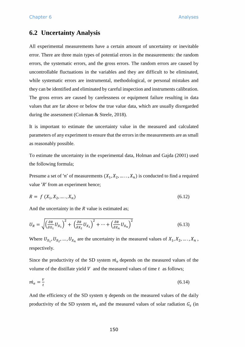
Chapter 6 Analyses
150
6.2 Uncertainty Analysis
All experimental measurements have a certain amount of uncertainty or inevitable
error. There are three main types of potential errors in the measurements: the random
errors, the systematic errors, and the gross errors. The random errors are caused by
uncontrollable fluctuations in the variables and they are difficult to be eliminated,
while systematic errors are instrumental, methodological, or personal mistakes and
they can be identified and eliminated by careful inspection and instruments calibration.
The gross errors are caused by carelessness or equipment failure resulting in data
values that are far above or below the true value data, which are usually disregarded
during the assessment (Coleman & Steele, 2018).
It is important to estimate the uncertainty value in the measured and calculated
parameters of any experiment to ensure that the errors in the measurements are as small
as reasonably possible.
To estimate the uncertainty in the experimental data, Holman and Gajda (2001) used
the following formula;
Presume a set of ‘𝑛’ of measurements (𝑋1, 𝑋2, … . . , 𝑋𝑛) is conducted to find a required
value ‘𝑅’ from an experiment hence;
𝑅 = 𝑓 (𝑋1, 𝑋2, … . , 𝑋𝑛) (6.12)
And the uncertainty in the 𝑅 value is estimated as;
𝑈𝑅 = √(𝜕𝑅
𝜕𝑋1𝑈𝑋1
)2
+ (𝜕𝑅
𝜕𝑋2𝑈𝑋2
)2
+ ⋯ + (𝜕𝑅
𝜕𝑋𝑛𝑈𝑋𝑛
)2
(6.13)
Where 𝑈𝑋1, 𝑈𝑋2
, … , 𝑈𝑋𝑛 are the uncertainty in the measured values of 𝑋1, 𝑋2, … . , 𝑋𝑛 ,
respectively.
Since the productivity of the SD system 𝑚𝑒 depends on the measured values of the
volume of the distillate yield 𝑉 and the measured values of time 𝑡 as follows;
𝑚𝑒 =𝑉
𝑡 (6.14)
And the efficiency of the SD system 𝜂 depends on the measured values of the daily
productivity of the SD system 𝑚𝑒 and the measured values of solar radiation 𝐺𝑠 (in

Chapter 6 Analyses
151
addition to the latent heat of evaporation 𝑙𝑣 and the surface area of the SD system 𝐴𝑠
which are considered constant values) as follows;
𝜂 =𝑚𝑒 ×𝑙𝑣
𝐴𝑠×𝐺𝑠 (6.15)
The uncertainty in the measured productivity 𝑈𝑚𝑒 of the SD system can be found from
the following relation (Holman & Gajda, 2001);
𝑈𝑚𝑒 = √(𝜕𝑚𝑒
𝜕𝑉𝑈𝑉)
2
+ (𝜕𝑚𝑒
𝜕𝑡𝑈𝑡)
2
(6.16)
In the same way, the uncertainty in the estimated efficiency 𝑈𝜂 of the SD system can
be found from the following relation;
𝑈𝜂 = √(𝜕𝜂
𝜕𝑚𝑒𝑈𝑚𝑒 )
2
+ (𝜕𝜂
𝜕𝐺𝑈𝐺𝑠
)2
(6.17)
Where 𝑈𝑉 , 𝑈𝑡, 𝑎𝑛𝑑 𝑈𝐺𝑠 are the uncertainties in the values of the measured volume of
the distillate yield, the values of the measured time, and the values of the measured
solar radiation; respectively.
The results showed that the maximum estimated uncertainty was ±4.6% and ±5.25%
for the productivity and efficiency, respectively. The full calculations of the
uncertainty analysis is presented in Appendix C.

Chapter 6 Analyses
152
6.3 Cost Analysis
The cost analysis was conducted for the NSD and the MSD systems under study, to
estimate the cost of the water produced by the NSD system and the MSD system, and
to find out if the modification of the MSD system is justified or not?
The Cost of the water produced Per Litre (𝐶𝑃𝐿) can be found from the following
equations (Rajaseenivasan & Srithar, 2016);
𝐶𝑃𝐿 = 𝑇𝐶 𝐴𝑌⁄ (6.18)
Where;
𝐴𝑌 = Average Yield in litres
𝑇𝐶 = Total Cost in AUD
The total cost of the NSD system is;
𝑇𝐶𝑁𝑆𝐷 = 𝐹𝐶 + 𝑀𝐶 − 𝑆𝑉 (6.19)
The total cost of the MSD system is;
𝑇𝐶𝑀𝑆𝐷 = 𝐹𝐶 + 𝑀𝐶 + 𝑃𝐶 − 𝑆𝑉 (6.20)
Where;
𝐹𝐶 = Fixed Cost (capital cost)
𝑀𝐶 = Maintenance Cost (for two years) ≅ 20% 𝐹𝐶
𝑆𝑉 = Salvage Value (resale value at the end of use) ≅ 20% 𝐹𝐶
𝑃𝐶 = Power Cost for the MSD system
Table 6.2 lists the fixed or the capital cost of the NSD system and the MSD system

Chapter 6 Analyses
153
Table 6. 2 The capital cost or the fixed cost FC of the NSD system and the MSD system
Item Quantity Cost ($AUD)
NSD MSD
Aluminium sheet (1200 mm ×2400 mm ×3 mm) 1 60 60
Plexiglas sheet (1220 mm ×2440 mm ×3 mm) 1 50 50
Insulation XPS foam board (1200 mm ×600 mm ×60 mm) 3 30 30
Worm-gear DC motor (12 V, 50 W, 29 Nm, 65 rpm) 3 120
Variable DC power supply (16 V, 25 A) 1 120
PVC pipe (90 mm × 3 m) 1 10
PVC push-on cap (90 mm) 6 15
Tubing, float, and other accessories sum 30 50
Total 170 455
If we assumed that;
1. The life span of both the SD systems is two years only.
2. Both the SD systems are working 300 days per year assuming 65 days per year
for the maintenance
And if we knew that;
3. The average daily productivity of the NSD system and the MSD system was
about 0.562 𝑙/𝑑𝑎𝑦 and 0.965 𝑙/𝑑𝑎𝑦, respectively
4. The energy consumed by the DC motors in the MSD system was about
50 𝑊𝑎𝑡t, they were working 12 hours per day, and the electricity cost is
0.1 $𝐴𝑈𝐷/𝑘𝑊ℎ𝑟
We can find that;
1. The 𝐴𝑌 of the NSD system and the MSD system during two years period will
be about 337.2 𝑙𝑖𝑡𝑟𝑒 and 579 𝑙𝑖𝑡𝑟𝑒, respectively
2. The 𝑃𝐶 =50 𝑊
1000× 12 ℎ𝑟 × 600 𝑑𝑎𝑦𝑠 × 0.1 $𝐴𝑈𝐷/𝑘𝑊ℎ𝑟 = 36 $𝐴𝑈𝐷
3. The 𝑇𝐶𝑁𝑆𝐷 = 170 $𝐴𝑈𝐷 and the 𝑇𝐶𝑀𝑆𝐷 = 455 + 36 = 491 $𝐴𝑈𝐷.
4. The 𝐶𝑃𝐿 of the NSD system and the MSD system will be (0.5 $AUD/l= 0.34
$USD/l) and (0.85 $AUD/l= 0.57 $USD/l), respectively. The exchange rate
from AUD to USD was 0.67.

Chapter 6 Analyses
154
According to the cost analysis, the capital or the fixed cost 𝐹𝐶 of the MSD system was
higher by 167.6% than the capital cost of the NSD system. The total cost 𝑇𝐶 of the
MSD system was higher by 188.8% than the total cost of the NSD system. The cost
of the water produced per litre 𝐶𝑃𝐿 of the MSD system was higher by 67.6% than that
of the NSD system. The cost analysis showed that the modification to the SD system
was unjustified even though the modification had increased the productivity (average
yield) 𝐴𝑌 of the SD system by an average of 71.7%. The reason for the increase in the
cost was the cost of the extra items required for the modification and the cost of the
power that was used to run the motors to rotate the tubes. It is worth mentioning that
the present SD systems used in this experiment were small-sized to fulfil the research
budget and the lifespan was considered to be only two years (other researchers
considered longer lifetime up to 30 years). Besides a longer lifespan, if the present
MSD system manufactured in a larger-scale the cost of the extra items that are required
for the modification will be diminished, thereby the price of the water produced by
this system will be much cheaper.

Chapter 7 Conclusions
155
7 Chapter Seven: Conclusions and
Recommendations
This chapter provides a summary of the thesis, presents the conclusions of this work,
and suggests recommendations for future work.
7.1 Thesis Summary
Water is an essential need, and there is an ethical obligation to provide all people with
clean and fresh water. Some more impoverished regions have limited, or no access to
potable water, especially the small communities that live in remote and arid areas.
Some of these areas have no resources or suitable infrastructure with which to build
desalination plants. In addition, transporting water to these remote areas is costly and
connecting these areas to the electricity grid that is needed to operate the desalination
plants may be a challenge. One of the simplest and most effective solutions is
employing abundant solar energy to run small and inexpensive solar desalination
systems. Solar Still Desalination (SD) systems consist of a basin of saline water
covered with a tilted transparent cover that is exposed to solar radiation. The solar
radiation heats the brackish water in the basin, producing vapour that condenses on the
inner surface of the cover providing fresh water. SD systems do not require
complicated maintenance or special skills to run. SD systems are very simple, low-
cost, can be constructed from locally available materials, and can be operated by
anyone. Despite the advantages of the SD systems, low productivity is the only
drawback of these systems.
Increasing the productivity of the SD systems is the main purpose of this study. The
proposed modification to achieve this goal was introducing three symmetrical and
parallel revolving tubes in the water basin of the SD system. The revolving tubes were
semi-immersed in the water in the basin. The Modified SD system (MSD) has
advantages over the Normal SD system (NSD) of adding extra surfaces for the water
evaporation, preventing water stagnation, and enhancing the solar absorption.
Increasing the surface area of evaporation led to an increase in the evaporation rate,

Chapter 7 Conclusions
156
which led to increases in productivity. Increasing the SD system productivity under
the same unit area means enhancing the efficiency of the SD system.
This study was conducted in the following sequence. Firstly, a CFD model using
ANSYS-FLUENT software was developed to simulate the NSD system and the MSD
system and to estimate the productivities of both systems to confirm the possibility of
the enhancement of performance. Then experimental tests for both the SD systems
were carried out in the University of Southern Queensland campus, Toowoomba,
Australia for about seven months from the 4th of October 2017 to the 23rd of April
2018. After validating the simulation results with the experimental data, the numerical
model was then employed to perform the sensitivity analysis for some design and
operation parameters. The uncertainty in the experimental measurements was
estimated for reliability. Finally, the cost analysis of both the SD systems was
implemented to justify the extra cost of the modification to the MSD system.
The conclusions of the present study and the recommendations for future work are
presented in the following sections.
7.2 Conclusions
After conducting the numerical simulation, the experimental investigation, the
sensitivity analysis, and the cost analysis to the MSD system and the NSD system, the
following conclusions were reached:
1. The maximum and the average daily productivity of the MSD system were
2.908 𝑙/𝑚2 and 2.011 𝑙/𝑚2 , respectively.
2. The maximum and the average daily productivity of the NSD system were
1.685 𝑙/𝑚2 and 1.172 𝑙/𝑚2 , respectively.
3. The daily productivity of the MSD system was higher than the daily
productivity of the NSD system by an average of 71.7%.
4. The maximum and the average daily efficiency of the MSD system were
21.01% and 18.77% , respectively.
5. The maximum and the average daily efficiency of the NSD system were
13.12% and 12.11% , respectively.

Chapter 7 Conclusions
157
6. The daily efficiency of the MSD system was higher than the daily efficiency
of the NSD system by an average of 54.3%.
7. The maximum enhancement in the daily productivity and in the daily
efficiency of the MSD system were 74.8% and 63.4% higher than the NSD
system, respectively.
8. The results of the CFD simulation showed a good agreement with the
experimental results with a maximum error of ±10%.
9. The numerical modelling using ANSYS- Fluent proved to be a successful tool
to simulate the SD system performance and to analyse the operation and design
parameters of the SD systems.
10. According to the sensitivity analysis, the increase in the solar radiation
intensity, the temperature of the feed water, the surface area, the diameter of
the revolving tubes, and the rotation speed of the revolving tubes have a
positive effect on the productivity of the SD systems.
11. According to the sensitivity analysis, the increase in the water depth, water
mass, and the temperature of the SD cover have a negative effect on the
productivity of the SD systems.
12. The initial or the capital cost of the MSD system and the NSD system were
$455 𝐴𝑈𝐷 and $170 𝐴𝑈𝐷 , respectively.
13. According to the cost analysis, the cost of the water produced by the MSD
system and the NSD system were $0.85 𝐴𝑈𝐷 = 0.57 $𝑈𝑆𝐷 𝑝𝑒𝑟 𝑙𝑖𝑡𝑟𝑒 and
$0.5 𝐴𝑈𝐷 = 0.34 $𝑈𝑆𝐷 𝑝𝑒𝑟 𝑙𝑖𝑡𝑟𝑒 , respectively.
14. According to the cost analysis, the capital cost of the MSD system was higher
by 167.6% than the capital cost of the NSD system, and the value of the
produced water by the MSD system was higher by 67.6% than the value of the
water produced by the NSD system.
In brief, the SD system has low productivity per unit area. The modification of the
revolving tubes that were added to the basin of the SD system had enhanced the
productivity of the system significantly. However, this modification was not cost-
effective due to the extra cost of the additional items and the cost of power required to
run the motors that rotate the tubes. Noting that, the size of the SD system was small
and the lifespan considered short being only two years. The effect of the cost of the

Chapter 7 Conclusions
158
power and the extra items on the cost of the produced water can be mitigated using a
bigger sized SD system and considering a longer working life.
7.3 Recommendations
Finally, the researcher would like to suggest the following recommendations for future
work:
1. Establish and conduct experimental tests to a more extensive sized SD system,
at least 1.5 𝑚 × 1 𝑚 or larger if possible. The reason is the larger system will
have higher productivity and the cost of the extra items required for the
modification would be close to the present system used in this work, which
may lead to decrease the cost of the water produced significantly.
2. Use revolving tubes wrapped with other alternative absorbent materials such
as a sponge layer or other porous materials and/or change the tube’s material
and/or the tube’s cross-section shape. The current research used PVC tubes
wrapped with a black absorbent mat. Using other materials or other tubes
configurations such as polygon tube may have a good effect on the productivity
of the SD system and will need to be tested experimentally to verify this
expectation.
3. Study the feasibility of using a small solar panel or a small wind turbine to run
the motors instead of electrical power. Using renewable sources to run the
motors may reduce the cost of the power, the power supply and the wiring. It
is more environmentally friendly and more practical for remote areas without
power connections.
4. Use other enhancements to the SD system in conjunction with the present
enhancement of the revolving tubes, such as reflective surfaces, heat
exchangers to preheat the feed water, and/or film cooling to reduce the cover
temperature. Using multiple enhancements or modifications in one system may
have a great combined effect on the productivity and it will require further
study.
5. Go further with dimensional analysis and Pi-groups to develop empirical
correlations.

References
159
References
Abdallah, S., & Badran, O. O. (2008). Sun tracking system for productivity
enhancement of solar still. Desalination, 220(1-3), 669-676.
Abdallah, S., Badran, O. O., & Abu-Khader, M. M. (2008). Performance evaluation
of a modified design of a single slope solar still. Desalination, 219(1-3), 222-
230.
Abdel-Rehim, Z. S., & Lasheen, A. (2007). Experimental and theoretical study of a
solar desalination system located in Cairo, Egypt. Desalination, 217(1-3), 52-
64.
Abu-Hijleh, B. A. K., & Rababa'h, H. M. (2003). Experimental study of a solar still
with sponge cubes in basin. Energy Conversion and Management, 44(9),
1411-1418.
Abu-Qudais, M., & Othman, O. N. (1996). Experimental study and numerical
simulation of a solar still using an external condenser. Energy, 21(10), 851-
855.
Ahmed, M. I., Hrairi, M., & Ismail, A. F. (2009). On the characteristics of multistage
evacuated solar distillation. Renewable Energy, 34(6), 1471-1478
Ahsan, A., Imteaz, M., Rahman, A., Yusuf, B., & Fukuhara, T. (2012). Design,
fabrication and performance analysis of an improved solar still. Desalination,
292, 105-112.
Ahsan, A., Imteaz, M., Thomas, U. A., Azmi, M., Rahman, A., & Daud, N. N.
(2014). Parameters affecting the performance of a low cost solar still. Applied
energy, 114, 924-930.
Akther, N., Sodiq, A., Giwa, A., Daer, S., Arafat, H. A., & Hasan, S. W. (2015).
Recent advancements in forward osmosis desalination: a review. Chemical
Engineering Journal, 281, 502-522.

References
160
Al-Hinai, H., Al-Nassri, M. S., & Jubran, B. A. (2002). Effect of climatic, design and
operational parameters on the yield of a simple solar still. Energy Conversion
and Management, 43(13), 1639-1650.
Al-Kharabsheh, S., & Yogi, D. (2003). Analysis of an innovative water desalination
system using low-grade solar heat. Desalination, 156(1-3), 323-332.
Al-Sulttani, A. O., Ahsan, A., Rahman, A., Daud, N. N., & Idrus, S. (2017). Heat
transfer coefficients and yield analysis of a double-slope solar still hybrid
with rubber scrapers: an experimental and theoretical study. Desalination,
407, 61-74.
Ansari, O., Asbik, M., Bah, A., Arbaoui, A., & Khmou, A. (2013). Desalination of
the brackish water using a passive solar still with a heat energy storage
system. Desalination, 324, 10-20.
Appadurai, M., & Velmurugan, V. (2015). Performance analysis of fin type solar still
integrated with fin type mini solar pond. Sustainable Energy Technologies
and Assessments, 9, 30-36.
Arunkumar, T., Jayaprakash, R., Denkenberger, D., Ahsan, A., Okundamiya, M. S.,
Tanaka, H., & Aybar, H. Ş. (2012). An experimental study on a
hemispherical solar still. Desalination, 286, 342-348.
Australian Water Association. (2009). Desalination Fact sheet. National Water
Week 18-24 October. Australia: AWA.
Baawain, M., Choudri, B. S., Ahmed, M., & Purnama, A. (Eds.). (2015). Recent
progress in desalination, environmental and marine outfall systems. Cham,
Switzerland: Springer.
Badran, O. O., & Abu-Khader, M. M. (2007). Evaluating thermal performance of a
single slope solar still. Heat and mass transfer, 43(10), 985-995.
Badran, O. O., & Al-Tahaineh, H. A. (2005). The effect of coupling a flat-plate
collector on the solar still productivity. Desalination, 183(1-3), 137-142.

References
161
Banat, F., & Jwaied, N. (2008). Economic evaluation of desalination by small-scale
autonomous solar-powered membrane distillation units. Desalination, 220(1-
3), 566-573.
Buckingham, E. (1914). On physically similar systems; illustrations of the use of
dimensional equations. Physical review, 4(4), 345.
Bureau of Meteorology, Australia. (2019). Latest Weather Observations for
Queensland. Retrieved from http://www.bom.gov.au/qld/observations/
Chorin, A. J. (1968). Numerical solution of the Navier-Stokes equations.
Mathematics of computation, 22(104), 745-762.
Coleman, H. W., & Steele, W. G. (2018). Experimentation, validation, and
uncertainty analysis for engineers. John Wiley & Sons.
Dashtban, M., & Tabrizi, F. F. (2011). Thermal analysis of a weir-type cascade solar
still integrated with PCM storage. Desalination, 279(1-3), 415-422.
Dev, R., Abdul-Wahab, & Tiwari, G. N. (2011a). Characteristic equation of the
inverted absorber solar still. Desalination, 269(1-3), 67-77.
Dev, R., Abdul-Wahab, S. A., & Tiwari, G. N. (2011b). Performance study of the
inverted absorber solar still with water depth and total dissolved solid.
Applied energy, 88(1), 252-264.
Dimri, V., Sarkar, B., Singh, U., & Tiwari, G. N. (2008). Effect of condensing cover
material on yield of an active solar still: an experimental validation.
Desalination, 227(1-3), 178-189.
Draper, N. R., & Smith, H. (2014). Applied regression analysis (Vol. 326). John
Wiley & Sons.
Duffie, J. A., & Beckman, W. A. (2013). Solar engineering of thermal processes.
John Wiley & Sons.

References
162
Dunkle, R. V. (1961). Solar water distillation: the roof type still and a multiple effect
diffusion still. In Proc. International Heat Transfer Conference, University of
Colorado, USA (Vol. 5, p. 895).
Dwivedi, V. K., & Tiwari, G. N. (2009). Comparison of internal heat transfer
coefficients in passive solar stills by different thermal models: an
experimental validation. Desalination, 246(1-3), 304-318.
Eakins, B.W., & Sharman, G.F. (2010). Volumes of the World's Oceans from
ETOPO1. National Geophysical Data Centre, Boulder. CO: NOAA.
Edalatpour, M., Aryana, K., Kianifar, A., Tiwari, G. N., Mahian, O., & Wongwises,
S. (2016). Solar stills: A review of the latest developments in numerical
simulations. Solar Energy, 135, 897-922.
El-Agouz, S. A. (2014). Experimental investigation of stepped solar still with
continuous water circulation. Energy Conversion and Management, 86, 186-
193.
El-Bahi, A., & Inan, D. (1999a). A solar still with minimum inclination, coupled to
an outside condenser. Desalination, 123(1), 79-83.
El-Bahi, A., & Inan, D. (1999b). Analysis of a parallel double glass solar still with
separate condenser. Renewable Energy, 17(4), 509-521
El-Mudir, W., El-Bousiffi, M., & Al-Hengari, S. (2004). Performance evaluation of a
small size TVC desalination plant. Desalination, 165, 269-279.
El-Samadony, Y. A. F., Abdullah, A. S., & Omara, Z. M. (2015). Experimental study
of stepped solar still integrated with reflectors and external condenser.
Experimental Heat Transfer, 28(4), 392-404.
El-Sebaii, A. A., Al-Ghamdi, A. A., Al-Hazmi, F. S., & Faidah, A. S. (2009).
Thermal performance of a single basin solar still with PCM as a storage
medium. Applied Energy, 86(7-8), 1187-1195.

References
163
El-Sebaii, A. A., Ramadan, M. R. I., Aboul-Enein, S., & Salem, N. (2008). Thermal
performance of a single-basin solar still integrated with a shallow solar pond.
Energy conversion and Management, 49(10), 2839-2848.
Eltawil, M. A., & Omara, Z. M. (2014). Enhancing the solar still performance using
solar photovoltaic, flat plate collector and hot air. Desalination, 349, 1-9.
Estahbanati, M. K., Ahsan, A., Feilizadeh, M., Jafarpur, K., Ashrafmansouri, S. S., &
Feilizadeh, M. (2016). Theoretical and experimental investigation on internal
reflectors in a single-slope solar still. Applied Energy, 165, 537-547.
Fatchurrohman, N., & Chia, S. T. (2017). Performance of hybrid nano-micro
reinforced mg metal matrix composites brake calliper: simulation approach.
Fourth International Conference on Mechanical Engineering Research, (Vol.
257, p. 012060). IOP.
Fath, H. E., El-Samanoudy, M., Fahmy, K., & Hassabou, A. (2003). Thermal-
economic analysis and comparison between pyramid-shaped and single-slope
solar still configurations. Desalination, 159(1), 69-79.
Fluent, A. (2017). ANSYS Fluent Theory Guide, Release 18.2. USA: ANSYS Inc.
Ghaffour, N., Bundschuh, J., Mahmoudi, H., & Goosen, M. F. (2015). Renewable
energy-driven desalination technologies: A comprehensive review on
challenges and potential applications of integrated systems. Desalination,
356, 94-114.
Gleick, P. H. (1993). Water in crisis: a guide to the world’s fresh water resources.
Oxford University Press.
Google Maps Australia. (2019). Retrieved from https://www.google.com/maps/
Goosen, M. F., Sablani, S. S., Shayya, W. H., Paton, C., & Al-Hinai, H. (2000).
Thermodynamic and economic considerations in solar desalination.
Desalination, 129(1), 63-89.

References
164
Gude, V. G., Nirmalakhandan, N., & Deng, S. (2010). Renewable and sustainable
approaches for desalination. Renewable and sustainable energy reviews,
14(9), 2641-2654.
Gupta, B., Sharma, R., Shankar, P., & Baredar, P. (2016). Performance enhancement
of modified solar still using water sprinkler: An experimental approach.
Perspectives in Science, 8, 191-194.
Helal, A. M., & Al-Malek, S. A. (2006). Design of a solar-assisted mechanical vapor
compression (MVC) desalination unit for remote areas in the UAE.
Desalination, 197(1-3), 273-300.
Hirunpinyopas, W., Prestat, E., Worrall, S. D., Haigh, S. J., Dryfe, R. A., & Bissett,
M. A. (2017). Desalination and nanofiltration through functionalized laminar
MoS2 membranes. ACS nano, 11(11), 11082-11090.
Holman, J. P., & Gajda, W. J. (2001). Experimental methods for engineers (Vol. 2).
NY: McGraw-Hill.
Huttner, K. R. (2013). Overview of existing water and energy policies in the MENA
region and potential policy approaches to overcome the existing barriers to
desalination using renewable energies. Desalination and Water Treatment,
51(1-3), 87-94.
Ibrahim, A. G., Allam, E. E., & Elshamarka, S. E. (2015). A modified basin type
solar still: Experimental performance and economic study. Energy, 93, 335-
342.
Ismail, B. I. (2009). Design and performance of a transportable hemispherical solar
still. Renewable Energy, 34(1), 145-150.
Jamil, B., & Akhtar, N. (2017). Effect of specific height on the performance of a
single slope solar still: An experimental study. Desalination, 414, 73-88
Kabeel, A. E. (2009). Performance of solar still with a concave wick evaporation
surface. Energy, 34(10), 1504-1509.

References
165
Kabeel, A. E., & Abdelgaied, M. (2016). Improving the performance of solar still by
using PCM as a thermal storage medium under Egyptian conditions.
Desalination, 383, 22-28.
Kabeel, A. E., & Abdelgaied, M. (2017). Observational study of modified solar still
coupled with oil serpentine loop from cylindrical parabolic concentrator and
phase changing material under basin. Solar Energy, 144, 71-78.
Kabeel, A. E., Omara, Z. M., & Essa, F. A. (2014a). Enhancement of modified solar
still integrated with external condenser using nanofluids: an experimental
approach. Energy conversion and management, 78, 493-498.
Kabeel, A. E., Omara, Z. M., & Essa, F. A. (2014b). Improving the performance of
solar still by using nanofluids and providing vacuum. Energy Conversion and
Management, 86, 268-274.
Kang, K. C., Linga, P., Park, K. N., Choi, S. J., & Lee, J. D. (2014). Seawater
desalination by gas hydrate process and removal characteristics of dissolved
ions (Na+, K+, Mg2+, Ca2+, B3+, Cl−, SO42−). Desalination, 353, 84-90.
Karagiannis, I. C., & Soldatos, P. G. (2008). Water desalination cost literature:
review and assessment. Desalination, 223(1-3), 448-456.
Khalifa, A. J. N. (2011). On the effect of cover tilt angle of the simple solar still on
its productivity in different seasons and latitudes. Energy conversion and
management, 52(1), 431-436.
Khalifa, A. J. N., & Hamood, A. M. (2009). Performance correlations for basin type
solar stills. Desalination, 249(1), 24-28.
Khalifa, A. J. N., & Ibrahim, H. A. (2009). Effect of inclination of the external
reflector on the performance of a basin type solar still at various seasons.
Energy for Sustainable Development, 13(4), 244-249.
Kianifar, A., Heris, S. Z., & Mahian, O. (2012). Exergy and economic analysis of a
pyramid-shaped solar water purification system: active and passive cases.
Energy, 38(1), 31-36.

References
166
Kim, S. E., Choudhury, D., & Patel, B. (1999). Computations of complex turbulent
flows using the commercial code FLUENT. In M. D. Salas, J. N. Hefner, &
L. Sakell (Eds.), Modeling complex turbulent flows (pp. 259-276). Dordrecht:
Springer- Science+ Business Medea.
Kleijnen, J. P. (2005). An overview of the design and analysis of simulation
experiments for sensitivity analysis. European Journal of Operational
Research, 164(2), 287-300.
Kumar, S., Dubey, A., & Tiwari, G. N. (2014). A solar still augmented with an
evacuated tube collector in forced mode. Desalination, 347, 15-24.
Lamei, A., Van der Zaag, P., & Von Muench, E. (2008). Impact of solar energy cost
on water production cost of seawater desalination plants in Egypt. Energy
Policy, 36(5), 1748-1756.
Launder, B. E., & Spalding, D. B. (1972). Mathematical models of turbulence.
Academic press.
Lee, W. H. (1979). A Pressure Iteration Scheme for Two-Phase Flow Modeling
(Technical Paper No. LA-UR-79-975). USA: Los Alamos National
Laboratory.
Lethea, L. (2017). Impact of water hardness on energy consumption of geyser
heating elements. Water SA, 43(4), 614-625.
Löhner, R. (2008). Applied computational fluid dynamics techniques: an
introduction based on finite element methods. John Wiley & Sons.
Malaiyappan, P., & Elumalai, N. (2016). Numerical investigations: basin materials of
a single-basin and single-slope solar still. Desalination and Water Treatment,
57(45), 21211-21233.
Malik, M. A. S., Tiwari, G. N., Kumar, A., & Sodha, M. S. (1982). Solar distillation:
a practical study of a wide range of stills and their optimum design,
construction, and performance. Oxford: Pergamon press.

References
167
Mamouri, S. J., Derami, H. G., Ghiasi, M., Shafii, M. B., & Shiee, Z. (2014).
Experimental investigation of the effect of using thermosyphon heat pipes
and vacuum glass on the performance of solar still. Energy, 75, 501-507.
Maroo, S. C., & Goswami, D. Y. (2009). Theoretical analysis of a single-stage and
two-stage solar driven flash desalination system based on passive vacuum
generation. Desalination, 249(2), 635-646.
Minocha, N., Joshi, J. B., Nayak, A. K., & Vijayan, P. K. (2016). 3D CFD simulation
of passive decay heat removal system under boiling conditions: Role of
bubble sliding motion on inclined heated tubes. Chemical Engineering
Science, 145, 245-265.
Monowe, P., Masale, M., Nijegorodov, N., & Vasilenko, V. (2011). A portable
single-basin solar still with an external reflecting booster and an outside
condenser. Desalination, 280(1-3), 332-338.
Moustafa, S. M. A., Jarrar, D. I., & El-Mansy, H. I. (1985). Performance of a self-
regulating solar multistage flash desalination system. Solar Energy, 35(4),
333-340.
Murugavel, K. K., Sivakumar, S., Ahamed, J. R., Chockalingam, K. K., & Srithar, K.
(2010). Single basin double slope solar still with minimum basin depth and
energy storing materials. Applied Energy, 87(2), 514-523.
Nafey, A. S., Abdelkader, M., Abdelmotalip, A., & Mabrouk, A. A. (2002).
Enhancement of solar still productivity using floating perforated black plate.
Energy Conversion and Management, 43(7), 937-946.
Omara, Z. M., Hamed, M. H., & Kabeel, A. E. (2011). Performance of finned and
corrugated absorbers solar stills under Egyptian conditions. Desalination,
277(1-3), 281-287.
Omara, Z. M., Kabeel, A. E., & Younes, M. M. (2014). Enhancing the stepped solar
still performance using internal and external reflectors. Energy conversion
and management, 78, 876-881.

References
168
Panchal, H. N., & Patel, S. (2017). An extensive review on different design and
climatic parameters to increase distillate output of solar still. Renewable and
sustainable energy reviews, 69, 750-758.
Panchal, H. N., & Shah, P. K. (2012). Effect of Varying Glass cover thickness on
Performance of Solar still: in a Winter Climate Conditions. International
Journal of Renewable Energy Research (IJRER), 1(4), 212-223.
Parekh, S., Farid, M. M., Selman, J. R., & Al-Hallaj, S. (2004). Solar desalination
with a humidification-dehumidification technique: a comprehensive technical
review. Desalination, 160(2), 167-186.
Peluffo, A., & Neger, Y. (2013). Seawater desalination: technical, environmental
and social aspects. Paris: Environmental Research and Teaching Institute,
CERES‐ERTI. Retrieved from
http://www.environnement.ens.fr/IMG/Desalination.pdf
Perlman, H. (2016). The distribution of water on, in, and above the Earth. Where is
Earth's water? USGS, Water science school. Retrieved from
https://www.usgs.gov/media/images/distribution-water-and-above-earth
Qiblawey, H. M., & Banat, F. (2008). Solar thermal desalination technologies.
Desalination, 220(1-3), 633-644.
Rahbar, N., & Esfahani, J. A. (2012). Experimental study of a novel portable solar
still by utilizing the heatpipe and thermoelectric module. Desalination, 284,
55-61.
Rahbar, N., & Esfahani, J. A. (2013). Productivity estimation of a single-slope solar
still: Theoretical and numerical analysis. Energy, 49, 289-297.
Rahbar, N., Esfahani, J. A., & Fotouhi-Bafghi, E. (2015). Estimation of convective
heat transfer coefficient and water-productivity in a tubular solar still–CFD
simulation and theoretical analysis. Solar Energy, 113, 313-323.

References
169
Rajaseenivasan, T., & Murugavel, K. K. (2013). Theoretical and experimental
investigation on double basin double slope solar still. Desalination, 319, 25-
32.
Rajaseenivasan, T., & Srithar, K. (2016). Performance investigation on solar still
with circular and square fins in basin with CO2 mitigation and economic
analysis. Desalination, 380, 66-74.
Rashidi, S., Akar, S., Bovand, M., & Ellahi, R. (2018). Volume of fluid model to
simulate the nanofluid flow and entropy generation in a single slope solar
still. Renewable Energy, 115, 400-410.
Rayan, M. A., Djebedjian, B., & Khaled, I. (2001). Water supply and demand and a
desalination option for Sinai, Egypt. Desalination, 136(1-3), 73-81.
Rijsberman, F. R. (2006). Water scarcity: fact or fiction?. Agricultural water
management, 80(1-3), 5-22.
Sadrzadeh, M., & Mohammadi, T. (2008). Sea water desalination using
electrodialysis. Desalination, 221(1-3), 440-447.
Sahota, L., & Tiwari, G. N. (2016). Effect of nanofluids on the performance of
passive double slope solar still: a comparative study using characteristic
curve. Desalination, 388, 9-21.
Sakthivel, M., Shanmugasundaram, S., & Alwarsamy, T. (2010). An experimental
study on a regenerative solar still with energy storage medium Jute cloth.
Desalination, 264(1-2), 24-31.
Sarray, Y., Hidouri, N., Mchirgui, A., & Brahim, A. B. (2017). Study of heat and
mass transfer phenomena and entropy rate of humid air inside a passive solar
still. Desalination, 409, 80-95.
Setoodeh, N., Rahimi, R., & Ameri, A. (2011). Modeling and determination of heat
transfer coefficient in a basin solar still using CFD. Desalination, 268(1-3),
103-110.

References
170
Shalaby, S. M., El-Bialy, E., & El-Sebaii, A. A. (2016). An experimental
investigation of a v-corrugated absorber single-basin solar still using PCM.
Desalination, 398, 247-255.
Sharaf, M. A., Nafey, A. S., & García-Rodríguez, L. (2011). Exergy and thermo-
economic analyses of a combined solar organic cycle with multi effect
distillation (MED) desalination process. Desalination, 272(1-3), 135-147.
Sharshir, S. W., Peng, G., Wu, L., Essa, F. A., Kabeel, A. E., & Yang, N. (2017).
The effects of flake graphite nanoparticles, phase change material, and film
cooling on the solar still performance. Applied energy, 191, 358-366.
Sharshir, S. W., Yang, N., Peng, G., & Kabeel, A. E. (2016). Factors affecting solar
stills productivity and improvement techniques: a detailed review. Applied
Thermal Engineering, 100, 267-284.
Shatat, M., Worall, M., & Riffat, S. (2013). Opportunities for solar water
desalination worldwide. Sustainable cities and society, 9, 67-80.
Singh, H. N., & Tiwari, G. N. (2004). Monthly performance of passive and active
solar stills for different Indian climatic conditions. Desalination, 168, 145-
150.
Slesarenko, V. V. (2001). Heat pumps as a source of heat energy for desalination of
seawater. Desalination, 139(1-3), 405-410.
Somwanshi, A., & Tiwari, A. K. (2014). Performance enhancement of a single basin
solar still with flow of water from an air cooler on the cover. Desalination,
352, 92-102.
Srivastava, P. K., & Agrawal, S. K. (2013a). Experimental and theoretical analysis of
single sloped basin type solar still consisting of multiple low thermal inertia
floating porous absorbers. Desalination, 311, 198-205.
Srivastava, P. K., & Agrawal, S. K. (2013b). Winter and summer performance of
single sloped basin type solar still integrated with extended porous fins.
Desalination, 319, 73-78.

References
171
Sun, D., Xu, J., & Chen, Q. (2014). Modeling of the evaporation and condensation
phase-change problems with FLUENT. Numerical Heat Transfer, Part B:
Fundamentals, 66(4), 326-342.
Tanaka, H., & Nakatake, Y. (2006). Theoretical analysis of a basin type solar still
with internal and external reflectors. Desalination, 197(1-3), 205-216.
Tiwari, A. K., & Tiwari, G. N. (2006). Effect of water depths on heat and mass
transfer in a passive solar still: in summer climatic condition. Desalination,
195(1-3), 78-94.
Tiwari, G. N. (2002). Solar energy: fundamentals, design, modelling and
applications. Alpha Science Int'l Ltd.
Tiwari, G. N., & Sahota, L. (2017). Review on the energy and economic efficiencies
of passive and active solar distillation systems. Desalination, 401, 151-179.
University of Southern Queensland. (2019). Toowoomba weather station. Retrieved
from http://foesweather.usq.edu.au/
Velmurugan, V., & Srithar, K. (2007). Solar stills integrated with a mini solar
pond—analytical simulation and experimental validation. Desalination,
216(1-3), 232-241.
Velmurugan, V., & Srithar, K. (2011). Performance analysis of solar stills based on
various factors affecting the productivity: a review. Renewable and
sustainable energy reviews, 15(2), 1294-1304.
Velmurugan, V., Deenadayalan, C. K., Vinod, H., & Srithar, K. (2008a).
Desalination of effluent using fin type solar still. Energy, 33(11), 1719-1727.
Velmurugan, V., Gopalakrishnan, M., Raghu, R., & Srithar, K. (2008b). Single basin
solar still with fin for enhancing productivity. Energy Conversion and
Management, 49(10), 2602-2608.
Velmurugan, V., Kumar, K. N., Haq, T. N., & Srithar, K. (2009). Performance
analysis in stepped solar still for effluent desalination. Energy, 34(9), 1179-
1186.

References
172
Versteeg, H. K., & Malalasekera, W. (2007). An introduction to computational fluid
dynamics: the finite volume method. Pearson education.
Wang, P., & Chung, T. S. (2015). Recent advances in membrane distillation
processes: Membrane development, configuration design and application
exploring. Journal of membrane science, 474, 39-56.
Welch, S. W., & Wilson, J. (2000). A volume of fluid based method for fluid flows
with phase change. Journal of computational physics, 160(2), 662-682.
White, F. M. (2016). Fluid mechanics (8th Ed.). NY: McGraw-Hill Education.
World Health Organization, & UNICEF. (2017). Progress on drinking water,
sanitation and hygiene: 2017 update and SDG baselines. Switzerland: JMP.
World Health Organization. (2011). Guidelines for drinking-water quality (4th Ed.).
Malta: Gutenberg.
Yang, Y., Shen, S., Zhou, S., Mu, X., & Zhang, K. (2015). Research for the
adjustable performance of the thermal vapour compressor in the MED–TVC
system. Desalination and Water Treatment, 53(7), 1725-1734.

Appendices
173
Appendix A: Figures
1. The temperature profile of selected days

Appendices
174

Appendices
175

Appendices
176

Appendices
177

Appendices
178

Appendices
179

Appendices
180

Appendices
181

Appendices
182

Appendices
183

Appendices
184
2. The hourly productivity of selected days

Appendices
185

Appendices
186

Appendices
187

Appendices
188

Appendices
189

Appendices
190

Appendices
191
3. The hourly efficiency of selected days

Appendices
192

Appendices
193

Appendices
194

Appendices
195
Appendix B: Tables
1. The recorded data of selected days of every month
The recorded data on the 4th of October 2017 Time Water Temperature
(°C)
Vapour
Temperature (°C)
Basin Temperature
(°C)
Cover Temperature
(°C)
Ambient
Tempera
ture (°C)
Wind
speed
(km/hr)
Relative
Humidit
y (%)
Solar
intensity
(W/m2) MSD NSD MSD NSD MSD NSD MSD NSD
6:00:00 20.1 22.5 19.3 20.7 20 21.4 19.2 19.8 19.4 0 98 21
6:05:00 20.1 22.5 19.1 20.4 20 21.4 18.9 19.7 19.2 0 98 28
6:10:00 20.1 22.4 19.1 20.6 20 21.4 18.9 19.7 19.5 0 98 33
6:15:00 20 22.4 19.1 20.6 20 21.4 19 19.7 19.4 3 98 42
6:20:00 20 22.4 19 20.6 19.9 21.4 18.9 19.7 19.4 2 98 54
6:25:00 19.9 22.3 19 20.5 19.8 21.3 18.6 19.6 19.4 0 98 51
6:30:00 20 22.3 19.4 20.7 19.9 21.3 18.8 19.6 19.4 0 98 74
6:35:00 20 22.3 19.2 20.6 19.9 21.3 18.8 19.8 19.4 0 98 84
6:40:00 20 22.2 19.4 20.8 19.9 21.3 19.3 19.9 19.5 0 98 69
6:45:00 19.9 22.2 19.5 21.1 19.9 21.2 19.4 20 19.5 0 98 93
6:50:00 20 22.2 19.5 21.2 20 21.3 19.7 20.1 19.5 5 98 128
6:55:00 20.1 22.3 19.9 21.5 20.1 21.4 20 20.3 19.6 6 98 137
7:00:00 20.1 22.2 19.7 21.5 20.1 21.3 19.6 20.4 19.6 2 98 155
7:05:00 20.2 22.3 19.8 21.3 20.3 21.5 19.5 20.5 19.7 0 98 178
7:10:00 20.3 22.3 20 21.5 20.4 21.5 19.8 20.5 19.7 2 98 178
7:15:00 20.2 22.3 20 21.5 20.3 21.4 19.9 20.3 19.4 2 98 278
7:20:00 20.4 22.4 20.3 22.6 20.6 21.6 20.3 21.4 20.1 8 98 186
7:25:00 20.6 22.5 20.9 22.7 20.7 21.7 20.5 21.3 20.1 5 98 220
7:30:00 20.6 22.5 22.2 23.8 20.8 21.8 20.3 22.2 20 2 98 172
7:35:00 20.7 22.7 25.6 27.4 21.2 22 21.2 23.7 20.3 3 98 169
7:40:00 20.9 22.8 26.7 31.3 21.6 22.2 21.7 24.2 20.4 0 98 178
7:45:00 21.2 23 24.5 28.2 22 22.7 21.5 23.4 20.4 5 98 195
7:50:00 21.8 23.4 24.7 28.3 22.5 23.2 21.8 23.6 20.7 0 98 227
7:55:00 22.3 23.5 23.1 25.7 22.7 23.4 21.6 22.8 20.3 2 98 239
8:00:00 22.6 23.7 25.6 29 23 23.4 21.7 23.4 20.8 3 98 207
8:05:00 22.8 24 30.1 34.2 23.5 23.6 23 25.5 21.1 5 98 243
8:10:00 23.2 24.2 29.6 33.8 24 24 23.6 26.6 22.2 5 97 211
8:15:00 23.7 24.6 28.9 33.3 24.6 24.5 23.9 25.9 21.6 2 97 288
8:20:00 24.5 24.7 25.7 28.4 25.1 25 22.6 24 20.8 5 97 237
8:25:00 24.9 25 26.2 28.9 25.3 25.1 22.8 24.2 21.6 2 96 216
8:30:00 25.2 25.4 30.3 34 25.5 25.1 23.9 26.3 22.3 0 96 246
8:35:00 25.6 25.6 29.2 33.1 26.1 25.4 23.9 25.9 21.9 0 96 274
8:40:00 26 25.9 32.6 36.5 26.5 25.6 24.4 27 22.7 0 96 295
8:45:00 26.7 26.3 31.6 35.3 27.2 26.1 24.6 26.3 22.3 0 95 336
8:50:00 27.2 26.7 35 39.5 27.8 26.5 25.9 28.7 23.7 0 94 315
8:55:00 27.6 27.1 35 40.1 28.4 27 26.1 28.9 23.1 0 93 257
9:00:00 28.3 27.5 36 41.3 29.2 27.7 26.7 29.6 23.7 0 91 257
9:05:00 29.2 27.9 36.7 41 29.8 28.3 26.8 29.6 23.3 0 90 336
9:10:00 29.9 28.3 36.2 40.3 30.5 28.8 27.2 30 23.6 5 90 404
9:15:00 30.7 28.7 36.7 41.2 31.1 29.1 27 29.5 23.3 5 89 234
9:20:00 31.4 29.1 34.1 37.2 31.8 29.4 26.3 28 22.3 0 87 299
9:25:00 32 29.5 37.6 41 32.1 29.6 27.4 29.9 23.6 3 87 387
9:30:00 32.5 29.8 37.1 40.8 32.9 29.7 27.3 29.3 23.7 0 87 380
9:35:00 33.1 30.1 38.3 41.9 33.2 30 27.8 30.3 23.9 13 87 311
9:40:00 33.7 30.6 39.5 43.8 33.9 30.3 28.7 31.3 24.1 8 86 308
9:45:00 34.4 31.1 41.3 45.2 34.9 30.9 29.7 32 24.9 3 87 364
9:50:00 35.3 31.4 36.9 39.1 35.5 31.5 28.2 29.6 23.5 2 86 606
9:55:00 35.9 32 40.5 44.3 36 31.8 29.3 31.5 24.4 6 87 508
10:00:00 36.5 32.4 41.4 44.9 36.6 32.1 29.8 31.9 24.5 10 87 1088
10:05:00 37.3 32.9 42.8 46.5 37.4 32.6 30.5 32.7 24.8 5 83 1021
10:10:00 38.1 33.3 43.2 46.7 38.2 33 31.1 33.1 25.4 10 83 1037
10:15:00 38.9 33.8 42.6 44.9 38.9 33.6 30.9 32.7 24.9 2 83 582
10:20:00 39.5 34.4 44.9 48.6 39.6 34 32.2 34.6 27 2 83 759
10:25:00 40.4 35 45.4 49.1 40.6 34.7 32.8 35.2 27.5 6 80 373
10:30:00 41.3 35.6 45.4 49.3 41.5 35.4 32.8 35.4 25.7 2 81 524
10:35:00 42.1 36.1 45.9 49.2 42.3 36.1 32.4 34.9 25.6 5 79 431
10:40:00 43 36.7 46.8 49.9 43.1 36.7 33 35.9 27 6 79 490
10:45:00 43.8 37.2 47.4 49.8 43.8 37.1 33 35.5 26 6 79 411
10:50:00 44.7 37.8 48.6 50.2 44.6 37.6 33.7 36.1 27.1 8 78 1266
10:55:00 45.5 38.3 49.3 50.5 45.3 38 33.6 35.6 26.2 8 77 515
11:00:00 46.1 38.8 50.1 51.5 46 38.4 34.7 37.1 28.1 8 77 594
11:05:00 46.9 39.3 50.5 51.3 46.7 38.8 34.9 37 27.5 6 77 1253
11:10:00 47.8 39.9 50.9 51.5 47.4 39.3 35.1 37.3 27.7 3 78 367
11:15:00 48.4 40.3 51.3 51.4 48 39.7 35.9 37.9 28.8 8 76 415
11:20:00 49.2 40.9 52.2 52.8 48.8 40.2 35.5 37.8 26.9 2 75 415
11:25:00 49.9 41.4 52.5 52.5 49.5 40.8 35.7 38.1 27.3 3 75 406
11:30:00 50.6 41.9 53.3 53.1 50.1 41.3 35.7 38.5 27.8 6 74 322
11:35:00 51.1 42.4 53.7 53.2 50.7 41.6 36.3 39.3 28.9 3 74 401
11:40:00 51.8 42.9 53.8 53.4 51.2 41.9 36.3 38.5 27.6 0 74 323
11:45:00 52.4 43.4 54.7 53.1 51.8 42.4 36.8 39.7 28.8 5 74 1208
11:50:00 53.1 43.8 55.3 53.8 52.3 42.7 37.1 38.8 26.8 3 74 1118

Appendices
196
Time Water Temperature
(°C)
Vapour
Temperature (°C)
Basin Temperature
(°C)
Cover Temperature
(°C)
Ambient
Tempera
ture (°C)
Wind
speed
(km/hr)
Relative
Humidit
y (%)
Solar
intensity
(W/m2) MSD NSD MSD NSD MSD NSD MSD NSD
11:55:00 53.7 44.4 55.7 53.9 52.9 43.1 37.2 38.8 27.1 8 70 1060
12:00:00 54.3 44.9 56.4 54.4 53.5 43.5 38.3 40.7 29.6 6 70 1069
12:05:00 54.7 45.3 56.5 54.5 54 43.7 38.5 41.2 29.5 0 69 1069
12:10:00 55.2 45.6 57 55 54.4 44 38.5 40.7 28.9 11 69 316
12:15:00 55.8 46.2 57.3 54.5 54.9 44.4 38.7 40.8 29 8 66 1055
12:20:00 56.3 46.5 57.5 54.5 55.1 44.5 38.4 39.5 27.5 13 69 1079
12:25:00 56.7 47 58.2 54.4 55.3 44.5 38.5 39.2 27.5 2 66 1090
12:30:00 57.2 47.3 57.6 54.7 55.7 44.5 38.3 39.4 27.4 3 68 1206
12:35:00 57.5 47.7 58.6 55.3 56.1 44.5 38.7 40.5 28.2 5 65 250
12:40:00 57.8 47.9 58.7 54.9 56.5 44.6 39.1 41.6 29.3 6 65 1058
12:45:00 58.1 48.2 60.1 55.7 56.9 44.9 39.8 42.2 29.5 0 64 1139
12:50:00 58.2 48.4 58.7 55 56.8 45.2 39.4 39.9 27.9 10 64 1076
12:55:00 58.5 48.7 59.2 56.4 57.1 45.3 39.8 41.4 29.2 5 63 1034
13:00:00 58.8 49 59.7 56.3 57.3 45.4 39.5 40.2 27.9 5 61 246
13:05:00 58.9 49.3 59.8 56.3 57.5 45.7 39.8 40.6 27.6 8 57 1009
13:10:00 59.2 49.6 59.5 56 57.8 45.8 40.3 41.7 29.7 6 62 1035
13:15:00 59.4 49.8 59.6 56.2 58 45.9 40 41.6 29.8 5 61 246
13:20:00 59.6 50 59 55.1 58.1 46.1 39.8 41.1 28.3 5 61 211
13:25:00 59.8 50.3 59.6 56.2 58.3 46.4 40.1 41.3 28.9 5 60 1002
13:30:00 59.9 50.6 59.7 56.3 58.5 46.5 40 41.5 29.6 3 59 972
13:35:00 60.1 50.7 59.5 55.3 58.5 46.5 39.8 41.3 28.9 11 59 933
13:40:00 60.2 50.9 60 55.4 58.6 46.6 40.1 41.9 29.2 8 59 193
13:45:00 60.4 51.1 59.6 55.2 58.7 46.7 40.5 41.3 29.2 3 60 886
13:50:00 60.4 51.3 59.7 55.2 58.7 46.7 40.1 40.8 28.9 3 58 896
13:55:00 60.3 51.4 59.5 55 58.8 46.7 40.6 42 29.8 5 56 882
14:00:00 60.4 51.5 59.2 55 58.8 46.7 40.6 40.9 28.5 8 56 831
14:05:00 60.3 51.6 58.9 54.8 58.8 46.8 40 41.2 28.7 11 55 139
14:10:00 60.3 51.7 58.7 54.5 58.8 46.9 39.9 40.9 29.2 10 58 167
14:15:00 60.2 51.8 59.1 55 58.7 46.8 40.1 41.4 29.1 6 56 195
14:20:00 60.2 51.8 58.8 54.6 58.6 46.8 40.6 42.1 30.1 2 53 185
14:25:00 60.1 51.9 58.4 54.3 58.6 46.8 40.2 41.6 29.6 3 56 749
14:30:00 60.1 51.9 58.2 53.8 58.5 46.9 40.5 41.8 30.1 2 51 754
14:35:00 59.9 51.9 57.9 54.4 58.5 46.9 39.9 41.4 29.1 3 52 754
14:40:00 59.7 52 57.4 53.8 58.1 46.9 39.9 40.2 28.7 3 48 155
14:45:00 59.6 52 57.6 54 58.1 46.8 40.2 41 28.8 8 48 701
14:50:00 59.5 52.2 57.3 53.9 58.1 46.9 40.5 41.9 30 10 49 661
14:55:00 59.5 52.2 56.9 53.5 57.9 47 39.9 40.6 29 3 49 633
15:00:00 59.2 52.3 56.5 53.8 57.7 47 40 41 28.4 8 48 589
15:05:00 58.9 52.3 56.1 53.3 57.3 46.9 39.1 39.3 27.4 2 44 566
15:10:00 58.7 52.4 55.6 52.8 57.2 46.9 39.9 40.3 28.8 3 44 557
15:15:00 58.4 52.3 55.2 52.9 57 46.7 39.6 40.3 28.3 2 45 526
15:20:00 58.2 52.3 54.9 53.4 56.6 46.6 39.1 39.4 27.3 5 44 499
15:25:00 57.7 52.3 54.3 53.4 56.3 46.5 38.8 39.1 27.7 8 44 485
15:30:00 57.6 52.3 54.2 53.4 56 46.5 38.6 39.4 27.5 6 42 471
15:35:00 57.4 52.1 53.6 52.8 55.7 46.3 38.8 39.6 28.4 3 45 457
15:40:00 57.1 52 54.1 52.7 55.5 46.2 39.1 39.8 28.7 8 44 438
15:45:00 56.8 51.8 53.7 52.3 55.1 46.1 38.1 37.8 26.5 2 44 420
15:50:00 56.4 51.7 53.2 52 54.7 45.8 37.9 37.7 26.9 3 43 399
15:55:00 56.1 51.4 53.1 52.1 54.4 45.6 38.6 39.3 28.3 5 43 380
16:00:00 55.7 51 52.5 51.6 54.1 45.3 38.4 38.9 27.8 6 42 366
16:05:00 55.4 50.7 52.4 51.8 53.8 45.1 38 38.7 27.8 2 39 346
16:10:00 55.1 50.5 52.2 51.5 53.6 44.9 38 38.4 27.8 3 45 338
16:15:00 54.7 50.1 51.8 50.9 53.2 44.6 37.4 37.4 27.1 2 44 308
16:20:00 54.4 49.8 51.5 51 53 44.4 37.7 38.2 27.8 0 44 294
16:25:00 54.1 49.5 51.3 47.9 52.6 44.2 37.1 37.4 26.8 0 43 271
16:30:00 53.9 49.3 51.2 47.8 52.4 44.1 36.6 37.3 26.8 6 44 248
16:35:00 54 49.7 50.9 47.3 52.1 43.9 36.7 36.6 27 5 44 229
16:40:00 53.6 49.7 49.1 45 51.7 43.6 35.6 36.6 27 0 44 207
16:45:00 53.2 49.5 48.7 44 51.2 43.3 35 36.1 26.8 3 43 188
16:50:00 53.2 49.5 47.3 44 51.1 43.4 34.8 36.1 27.3 2 44 174
16:55:00 52 48.7 46.4 43.2 50 42.7 34 36.1 26.8 2 45 151
17:00:00 51 48.1 45.2 42.7 49 42.1 33.3 34.9 26.3 0 43 128
17:05:00 50.1 47.7 44.6 42.4 48.1 41.6 33.1 34.1 25.8 2 42 111
17:10:00 49.4 47.2 43.7 41.5 47.4 41.2 32.9 34.2 26 0 42 88
17:15:00 48.7 46.8 42.8 41.3 46.7 40.9 32.2 33.9 25.7 0 44 72
17:20:00 47.9 46.2 42 41.1 46 40.4 31.8 33.8 25.8 0 43 56
17:25:00 47.1 45.8 41.4 40.3 45.3 40 31.4 32.8 25 0 44 42
17:30:00 46.4 45.3 40.6 39.6 44.6 39.6 31.3 32.8 25.3 0 44 32
17:35:00 45.8 45 39.5 39 44 39.3 30.6 32 24.6 0 46 23
17:40:00 45.1 44.6 39.2 38.4 43.4 39 30.4 31.7 24.6 11 54 18
17:45:00 44.4 44.2 38.6 38.3 42.7 38.6 29.9 31.7 24.3 6 58 14
17:50:00 43.8 43.7 38.3 38.1 42.2 38.2 29.6 31.1 24.2 8 61 11
17:55:00 43.3 43.3 37.7 37.3 41.5 37.8 29.2 30.1 23.6 14 64 7
18:00:00 42.6 42.9 36.9 36.9 40.9 37.4 28.7 29.9 23.7 14 64 7
18:05:00 42 42.6 36.7 36.7 40.3 37.1 28.7 30.2 23.6 8 67 7
18:10:00 41.4 42.2 36.1 36.4 39.8 36.7 28.5 29.8 23.4 8 68 0
18:15:00 40.8 41.8 35.3 36 39.3 36.4 28 29.5 23.3 11 68 0
18:20:00 40.3 41.4 34.9 35.5 38.7 36.1 27.9 29 22.9 5 69 0
18:25:00 39.8 41 34.3 35.2 38.3 35.8 27.5 28.8 23 6 69 0

Appendices
197
Time Water Temperature
(°C)
Vapour
Temperature (°C)
Basin Temperature
(°C)
Cover Temperature
(°C)
Ambient
Tempera
ture (°C)
Wind
speed
(km/hr)
Relative
Humidit
y (%)
Solar
intensity
(W/m2) MSD NSD MSD NSD MSD NSD MSD NSD
18:30:00 39.2 40.6 33.9 35.1 37.7 35.5 27.4 28.7 22.8 14 70 0
18:35:00 38.7 40.3 33.3 34.4 37.2 35.1 27 28.2 22.7 18 71 0
18:40:00 38.3 39.9 32.8 33.8 36.7 34.8 26.6 27.5 22.4 16 75 0
18:45:00 37.7 39.6 32.4 33.9 36.4 34.6 26.5 27.7 22.6 11 79 0
18:50:00 37.2 39.2 32.1 33.6 35.9 34.2 26.3 27.5 22.5 19 82 0
18:55:00 36.9 39 31.7 33.6 35.4 34 26 27.1 22.2 13 84 0
19:00:00 36.3 38.5 31.5 33.4 34.9 33.7 25.8 27 22.2 24 85 0
19:05:00 36 38.4 30.8 32.9 34.6 33.5 25.5 26.8 22.2 21 86 0
19:10:00 35.5 37.9 30.5 32.1 34.2 33.2 25.3 26.3 21.7 16 87 0
19:15:00 35.1 37.7 30.3 31.5 33.8 33 25 26.5 22 13 88 0
19:20:00 34.7 37.4 29.5 31.5 33.4 32.7 24.6 25.8 21.6 24 89 0
19:25:00 34.3 37.1 29.4 31 33 32.4 24.3 25.6 21.5 13 89 0
19:30:00 33.9 36.7 28.8 30.9 32.6 32.1 24 25.5 21.2 10 90 0
19:35:00 33.5 36.4 28.3 31 32.3 31.9 24 25.4 21.1 11 90 0
19:40:00 33.1 36.2 28.4 30.5 32 31.7 23.9 25.2 21.2 23 90 0
19:45:00 32.7 35.9 28.2 30.2 31.6 31.4 23.7 24.9 20.9 14 90 0
19:50:00 32.3 35.5 27.7 30.7 31.2 31.2 23.5 24.9 20.8 13 91 0
19:55:00 32.1 35.3 27.8 30.6 31 31 23.7 24.7 20.7 14 92 0
20:00:00 31.7 35 27.3 30.2 30.6 30.7 23.9 24.8 20.9 16 92 0
20:05:00 31.4 34.8 27.2 30.1 30.4 30.5 24 24.5 20.6 21 93 0
20:10:00 31.1 34.5 27.2 29.6 30.1 30.4 24.1 24.9 20.8 14 93 0
20:15:00 30.9 34.3 27 29.5 29.9 30.2 24 24.8 20.8 23 93 0
20:20:00 30.6 34.1 26.7 29.3 29.6 30 23.9 24.4 20.5 11 94 0
20:25:00 30.4 33.9 26.8 29 29.5 30 24 24.3 20.7 16 94 0
20:30:00 30.1 33.7 26.5 29.2 29.2 29.8 23.7 24.2 20.4 11 94 0
20:35:00 29.8 33.4 26 28.7 28.9 29.6 23.4 24.2 20.5 13 94 0
20:40:00 29.7 33.3 25.7 28.4 28.7 29.5 22.7 23.6 20.3 18 94 0
20:45:00 29.3 33 25.3 28.3 28.5 29.3 22.2 23.2 20 14 95 0
20:50:00 29.1 32.8 25.1 27.4 28.2 29.1 21.7 22.9 19.8 14 95 0
20:55:00 28.8 32.6 24.6 27.1 27.9 28.8 21.4 22.7 19.9 19 95 0
21:00:00 28.6 32.3 24.6 27.2 27.7 28.6 21.3 22.6 19.7 14 95 0
21:05:00 28.2 32.1 24.3 26.8 27.4 28.3 21.1 22.5 19.8 18 95 0
21:10:00 27.9 31.8 24 27 27.1 28.2 21 22.4 19.6 24 95 0
21:15:00 27.7 31.6 23.9 26.8 26.9 27.9 20.9 22.2 19.6 19 95 0
21:20:00 27.5 31.4 23.6 26.1 26.7 27.8 20.7 21.9 19.6 21 96 0
21:25:00 27.3 31.2 23.3 26.1 26.5 27.6 20.6 21.9 19.5 16 95 0
21:30:00 26.9 30.9 23.2 26.1 26.1 27.4 20.3 21.7 19.4 23 96 0
21:35:00 26.7 30.7 22.9 26 25.9 27.2 20.3 21.6 19.4 23 96 0
21:40:00 26.6 30.6 22.9 25.6 25.8 27.1 20.3 21.6 19.4 18 96 0
21:45:00 26.3 30.4 22.8 25.6 25.6 27 20.2 21.5 19.4 14 96 0
21:50:00 26.1 30.2 22.4 25.3 25.4 26.8 20.1 21.4 19.3 18 96 0
21:55:00 25.9 29.9 22.4 25.1 25.2 26.6 20 21.1 19.1 19 96 0
22:00:00 25.7 29.7 22.1 25 25 26.4 19.8 21 19.1 19 96 0
22:05:00 25.4 29.5 22 24.9 24.8 26.2 19.7 20.9 19.1 14 96 0
22:10:00 25.3 29.3 21.9 24.6 24.6 26.1 19.6 20.9 19 16 96 0
22:15:00 25.1 29.2 21.8 24.5 24.4 26 19.5 20.7 18.9 13 96 0
22:20:00 24.8 29 21.6 24.3 24.2 25.8 19.3 20.6 18.9 18 96 0
22:25:00 24.7 28.8 21.6 24.2 24.1 25.7 19.3 20.7 19.1 16 96 0
22:30:00 24.4 28.5 21.2 23.8 23.8 25.5 19.1 20.4 18.7 18 96 0
22:35:00 24.3 28.4 21.2 23.7 23.7 25.4 19 20.3 18.7 14 96 0
22:40:00 24.1 28.2 21 23.7 23.5 25.2 18.9 20.1 18.7 21 96 0
22:45:00 24 28.1 20.9 23.6 23.4 25.2 18.9 20.3 18.7 14 96 0
22:50:00 23.8 27.9 20.9 23.3 23.2 24.9 18.8 20 18.6 16 96 0
22:55:00 23.5 27.7 20.5 23.2 23 24.8 18.7 19.9 18.7 16 96 0
23:00:00 23.4 27.5 20.4 23.1 22.9 24.6 18.5 19.8 18.5 18 96 0
23:05:00 23.3 27.4 20.4 23 22.7 24.5 18.6 19.8 18.5 18 96 0
23:10:00 23.1 27.2 20.2 23.1 22.6 24.4 18.4 19.7 18.4 14 96 0
23:15:00 23 27.1 20.2 23.1 22.5 24.3 18.4 19.7 18.5 16 96 0
23:20:00 22.8 26.9 19.9 22.8 22.3 24.2 18.2 19.6 18.4 21 96 0
23:25:00 22.7 26.7 20 22.6 22.2 24.1 18.2 19.6 18.4 18 96 0
23:30:00 22.5 26.6 19.8 22.5 22 23.9 18.6 19.5 18.3 14 96 0
23:35:00 22.4 26.5 20.2 23 21.9 23.9 19.4 19.9 18.5 19 96 0
23:40:00 22.3 26.3 20.2 22.8 21.8 23.7 19.1 19.7 18.5 14 96 0
23:45:00 22.1 26.2 20 22.7 21.7 23.7 19.3 19.9 18.6 16 96 0
23:50:00 22.1 26 19.9 22.6 21.6 23.6 19.2 19.9 18.6 16 96 0
23:55:00 21.9 25.9 19.8 22.2 21.5 23.5 18.6 19.7 18.5 19 96 0
0:00:00 21.8 25.8 19.6 22.2 21.6 23.4 18.2 19.5 18.5 19 96 0

Appendices
198
The recorded data on the 5th of November 2017 Time Water Temperature
(°C)
Vapour
Temperature (°C)
Basin Temperature
(°C)
Cover Temperature
(°C)
Ambient
Temperatur
e (°C)
Wind
speed
(km/hr)
Relative
Humidit
y (%)
Solar
intensit
y
(W/m2)
MSD NSD MSD NSD MSD NSD MSD NSD
6:00:00 12.5 15.8 11.6 13.2 12.6 14.7 10.8 12.5 13.7 8 70 141
6:05:00 12.5 15.8 11.7 13.3 12.6 14.6 10.8 12.5 13.7 5 71 160
6:10:00 12.5 15.7 11.7 13.3 12.6 14.6 11 12.6 13.7 6 72 183
6:15:00 12.4 15.6 11.8 13.2 12.5 14.6 11.1 12.7 13.7 10 72 206
6:20:00 12.4 15.6 11.8 13.4 12.5 14.6 11.1 12.7 13.8 8 72 227
6:25:00 12.3 15.5 11.8 13.2 12.5 14.5 11.3 12.8 13.8 3 71 246
6:30:00 12.3 15.4 11.8 13.4 12.4 14.5 11.1 12.8 14 10 70 265
6:35:00 12.3 15.5 11.9 13.4 12.5 14.5 11.2 12.9 14.1 10 69 285
6:40:00 12.2 15.3 11.8 13.3 12.5 14.5 11 12.9 14.1 10 70 304
6:45:00 12.3 15.4 11.8 13.4 12.5 14.6 11.3 13 14.4 5 70 322
6:50:00 12.2 15.4 11.9 13.5 12.5 14.6 11.4 13.2 14.6 8 70 330
6:55:00 12.2 15.3 11.9 13.3 12.5 14.5 11.4 13.3 14.8 10 70 44
7:00:00 12.3 15.3 12 13.4 12.6 14.6 11.7 13.4 15 5 70 141
7:05:00 12.3 15.3 12.1 13.7 12.6 14.6 12 13.7 15.4 5 70 399
7:10:00 12.4 15.3 12.4 14.2 12.6 14.6 13.5 15.8 15.7 3 69 418
7:15:00 12.4 15.4 12.4 17.9 12.7 14.7 14.4 17.1 15.5 5 68 434
7:20:00 12.3 15.5 15.3 19.4 12.8 14.9 14.9 18.2 15.8 5 68 454
7:25:00 12.3 15.7 16.6 21.2 13.3 15.3 15.1 18.9 16.2 5 67 471
7:30:00 12.5 15.8 18.2 24.8 13.6 15.8 15.8 19.6 16.6 11 67 490
7:35:00 12.7 16 20.9 25.5 14 16.2 16.9 19.7 16.6 10 67 510
7:40:00 13 16.2 21.6 26.2 14.4 16.5 17.8 20.5 17.5 5 66 527
7:45:00 13.5 16.6 22.2 26.8 14.8 16.9 18.3 21.1 17.9 8 65 561
7:50:00 14 16.8 23 27.6 15.4 17.3 18.4 21.4 18 11 65 577
7:55:00 14.6 17.2 23.6 28.1 16.1 17.8 18.7 21.9 18 8 64 596
8:00:00 15.3 17.6 24.2 31.1 16.8 18.2 19 21.8 17.7 8 64 613
8:05:00 16.1 18.1 25 32 17.4 18.7 19.7 22.4 18.3 6 63 471
8:10:00 16.7 18.4 26.1 32.4 18 19.1 20.1 23 19.1 14 62 121
8:15:00 17.4 18.9 27.2 33.4 18.8 19.6 20.8 23.8 19.7 6 65 645
8:20:00 18.2 19.3 28 34.2 19.5 20.1 21.3 24 19.5 11 63 677
8:25:00 18.9 19.7 28.5 34.7 20.2 20.5 21.5 24.2 19.5 13 63 693
8:30:00 19.7 20.2 29 35.4 20.9 20.9 21.7 24.1 19.2 10 65 708
8:35:00 20.6 20.6 29.8 35.7 21.6 21.4 22.1 24.5 19.7 10 64 722
8:40:00 21.3 21.1 30.4 36.1 22.4 21.7 22.4 24.6 19.6 13 63 737
8:45:00 22.4 21.6 31 36.7 23.1 22.1 22.6 25.2 20.2 8 62 752
8:50:00 23 22.1 31.5 37.6 23.9 22.5 23 25.6 20.5 14 62 768
8:55:00 23.9 22.6 32 37.9 24.7 22.9 23.3 25.6 20 16 63 779
9:00:00 24.7 23 33.1 38.6 25.3 23.3 23.6 26 20.3 19 61 796
9:05:00 25.4 23.5 33.4 39.3 26.1 23.7 24 26.8 21.3 8 60 819
9:10:00 26.2 23.9 33.8 38.9 26.8 23.9 24.2 26.5 20.7 10 61 802
9:15:00 26.9 24.4 35.6 40.8 27.7 24.4 25.2 27.8 21.6 11 60 744
9:20:00 27.9 25 35.5 40.8 28.5 25 25.5 27.6 21.1 3 60 371
9:25:00 28.7 25.4 35.9 41.1 29.3 25.5 26 28.5 21.9 8 60 872
9:30:00 29.6 25.8 36.9 41.3 30.2 26 25.9 28.2 20.7 10 57 867
9:35:00 30.5 26.5 37.7 41.9 31 26.5 26.5 29.1 22.4 5 58 872
9:40:00 31.3 27 38 42.8 31.8 26.9 26.6 28.9 21.9 14 56 884
9:45:00 32.3 27.5 38.8 43.3 32.5 27.2 26.7 28.8 21.4 11 55 893
9:50:00 33.2 28.2 38.8 43.2 33.3 27.7 27.1 29 21.9 10 55 422
9:55:00 33.9 28.6 40.2 44.5 34.1 28.2 27.7 30.1 23.3 5 55 907
10:00:00 34.9 29.1 40.3 45.2 34.9 28.6 27.7 29.7 21.7 19 52 916
10:05:00 35.6 29.7 41.3 45.4 35.7 29.2 28.1 30.3 22 3 54 918
10:10:00 36.5 30.3 41.7 45.2 36.4 29.7 28.3 30.1 22.3 5 52 933
10:15:00 37.4 30.8 42 46.1 37.2 30 28.8 30.6 22.8 10 52 939
10:20:00 38.2 31.4 42.6 46.5 38.1 30.5 29 30.8 22.5 10 51 944
10:25:00 39.1 31.9 43.6 47.1 38.8 30.9 29.3 30.9 22.4 8 49 947
10:30:00 39.8 32.5 44.3 47.5 39.6 31.4 30.1 31.8 23.1 8 49 949
10:35:00 40.7 33 44.9 47.7 40.4 31.8 29.8 31.4 22.5 3 48 954
10:40:00 41.5 33.6 45.4 47.9 41.1 32.3 30.5 32 23.3 10 46 962
10:45:00 42.3 34.1 45.7 48.3 41.8 32.7 30.9 32.6 23.8 6 47 970
10:50:00 43.1 34.5 46.4 49 42.6 33.2 31.3 32.7 23.9 3 46 981
10:55:00 43.8 35.1 47.5 48.7 43 33.5 31.2 32 23 11 45 990
11:00:00 44.5 35.6 48.1 49.9 44 34 32.2 33.5 23.9 6 43 990
11:05:00 45.4 36.1 48.5 49.1 44.9 34.5 32.5 34 24.5 11 41 990
11:10:00 46.1 36.6 49.4 48.7 45.3 35 32.6 33.6 24 10 39 1009
11:15:00 46.9 37.3 49.4 49.5 46.2 35.5 32.9 34.2 24.9 5 40 1005
11:20:00 47.6 37.7 49.5 50 46.8 35.8 32.8 33.6 23.6 2 38 1020
11:25:00 48.2 38.2 49.4 50.6 47.4 36.2 34 35.1 25.4 8 35 1016
11:30:00 48.9 38.7 51 51 48.1 36.7 34.3 35.4 25.4 11 35 1007
11:35:00 49.7 39.3 51.6 51.2 48.9 37.2 34.7 36.5 26.5 18 34 1021
11:40:00 50.2 39.8 51.8 51.4 49.5 37.8 34.4 36 25.2 13 34 1021
11:45:00 51 40.3 51.4 49.8 50 38.3 34.1 34.7 24.5 11 35 1032
11:50:00 51.5 40.8 53.1 51.8 50.6 38.6 34.4 35.7 24.7 0 35 1032
11:55:00 52.2 41.3 53.4 52.1 51.2 39.1 35 35.9 25 3 33 1037
12:00:00 52.7 41.8 53.5 52.2 51.7 39.5 35.2 36.1 25 14 34 1062
12:05:00 53.2 42.2 55.6 53.5 52.3 39.8 36.5 38.4 27.4 10 35 1053

Appendices
199
Time Water Temperature
(°C)
Vapour
Temperature (°C)
Basin Temperature
(°C)
Cover Temperature
(°C)
Ambient
Temperatur
e (°C)
Wind
speed
(km/hr)
Relative
Humidit
y (%)
Solar
intensit
y
(W/m2)
MSD NSD MSD NSD MSD NSD MSD NSD
12:10:00 53.8 42.6 55.5 53 52.7 40.1 36.2 37.4 26.6 10 34 1002
12:15:00 54.3 43.1 55.7 53.3 53 40.3 36 36.5 25.8 11 33 997
12:20:00 54.8 43.5 56.1 53.3 53.4 40.5 36.9 37.5 27.2 6 34 998
12:25:00 55.4 43.9 56.5 54 54.1 40.7 36.7 37.6 25.8 6 35 1025
12:30:00 55.9 44.4 56.6 53.3 54.4 41 37 37.9 26.2 2 34 410
12:35:00 56.2 44.8 58 54.2 55 41.3 37.9 39.1 26.6 10 34 213
12:40:00 56.7 45.3 58.4 54.2 55.2 41.5 37.8 37.9 26.1 14 35 183
12:45:00 57.1 45.7 57.6 53.7 55.3 41.6 37 36.8 24.8 8 36 211
12:50:00 57.4 46 57.5 54.3 55.7 41.6 37.7 37.7 25.9 2 38 346
12:55:00 57.8 46.3 58.6 54.8 56.1 41.9 37.9 38.9 27.3 11 36 1027
13:00:00 58.1 46.7 59.3 55.8 56.4 42.1 38.6 39 26.9 8 38 1035
13:05:00 58.3 46.8 57.2 46.9 56.7 42.4 37.6 37.6 25.6 14 36 230
13:10:00 58.4 47.1 59.6 49.9 56.8 42.4 38.6 38.9 26.4 11 34 204
13:15:00 58.6 47.3 59.3 51.2 57 42.6 38.5 39.3 26.5 11 34 229
13:20:00 58.8 47.6 59.4 54.8 57.2 42.8 38.4 38.4 25.8 16 31 155
13:25:00 59.1 48 59.4 55 57.5 43.2 39.1 39.8 27.4 10 31 148
13:30:00 59.3 48.4 61.1 52.2 58.1 43.5 40.5 40.4 27.7 6 32 172
13:35:00 59.8 48.8 61.4 52.5 58.5 44.1 40.6 41.3 27.3 10 32 172
13:40:00 60.2 49.2 62.1 53 58.9 44.6 40.6 41.1 27.2 2 32 186
13:45:00 60.7 49.4 57.8 50.3 58.8 45.1 37.7 38.3 25 13 31 185
13:50:00 60.6 49.7 59.4 54 59.1 45 39.2 40 27 5 31 169
13:55:00 60.8 49.9 57.5 49.9 58.9 45.1 36.6 37.4 24.6 6 31 830
14:00:00 60.4 49.7 56.3 48 58.3 44.9 36.4 36.6 24 6 30 814
14:05:00 59.5 49.5 57.9 51.5 57.3 44.1 37.8 38.2 25 3 29 807
14:10:00 59.3 49.5 59.9 55.8 57.6 43.6 39.7 40.1 26.5 3 28 791
14:15:00 59.3 49.7 59.9 56.3 57.8 43.5 39.9 40.1 26.7 11 27 779
14:20:00 59.5 49.8 58.8 54.9 57.8 43.9 39.1 38.6 25.6 16 27 754
14:25:00 59.6 49.9 55.6 48.8 57.4 44.2 36.9 36.8 24.4 16 26 735
14:30:00 59.1 49.8 57.6 52.9 57 43.8 38.7 38.9 26.1 6 28 717
14:35:00 58.8 49.7 57.7 53.2 56.9 43.4 39 39 26.6 8 27 712
14:40:00 58.7 49.7 57.2 53.2 57.1 43.4 38.1 38 24.8 21 26 700
14:45:00 58.7 49.9 57.2 52.6 57.1 43.6 38.6 37.8 25.1 2 26 682
14:50:00 58.5 49.8 55.5 50.3 56.6 43.8 38 38.7 26.1 6 26 673
14:55:00 58.1 49.8 56.2 52.3 56.6 43.7 37.8 38.2 26.3 6 27 661
15:00:00 58.3 50 54.1 47.6 56.6 44 37.1 38 25.6 23 26 645
15:05:00 57.6 49.8 55 51.1 55.9 43.7 37.7 37.7 25.6 23 26 635
15:10:00 57 49.6 55.2 52.8 55.5 43.6 38.4 39.2 26.3 16 27 608
15:15:00 56.8 49.7 55.1 52.6 55.4 43.5 38.1 38.3 26 6 28 585
15:20:00 57.1 49.8 52.4 46.3 55.3 43.9 35.7 37.3 24.9 10 28 571
15:25:00 56 49.4 52.8 50.5 54.3 43.6 37.3 36.8 25.2 3 29 568
15:30:00 55.7 49.3 52.2 49.4 54 43.2 37.2 37.6 26 10 29 529
15:35:00 55.2 49.2 51.9 50.5 53.8 43.2 36.6 36.8 24.9 14 29 503
15:40:00 55 49.1 51.3 50 53.5 43.2 36.6 36.9 24.8 16 30 487
15:45:00 54.7 49.1 51.5 49.9 53.2 43.1 36.4 36.7 24.8 11 30 469
15:50:00 54.5 49 51.5 49.6 52.8 43 36.4 36.4 25.2 11 32 457
15:55:00 54.3 48.7 51.9 50.1 52.8 42.9 36.5 36.9 25 19 32 436
16:00:00 54 48.5 51.6 50.4 52.6 42.5 36.5 36.2 24 14 33 142
16:05:00 53.9 48.3 50.8 48.5 52.3 42.3 35.7 36.2 24.6 19 33 302
16:10:00 53.6 48 50.3 48.3 52 41.9 35.5 36.2 24.2 19 34 76
16:15:00 53.4 47.7 49.7 47.9 51.7 41.7 34.7 35.9 24.5 31 34 79
16:20:00 53.2 47.4 49.7 47.9 51.4 41.3 34.9 36.1 24.5 23 35 76
16:25:00 53 47.2 49.5 47.6 51.2 40.9 35 35.6 24.2 19 36 84
16:30:00 52.9 47.4 49.4 47.9 51.2 41 34.9 35.4 24.3 26 36 70
16:35:00 53 48.1 49.7 48.6 51.3 41.6 35 35.8 24.5 19 35 56
16:40:00 53 48.3 48.7 47.1 51.2 41.5 34.1 34.8 23.6 14 35 60
16:45:00 52.3 48 46.5 43.1 50.4 41.4 33.1 34.5 23.7 14 35 62
16:50:00 52 47.9 48.8 47 50.2 41.2 33.6 34.3 23.4 21 35 104
16:55:00 51.8 47.7 48.6 44.4 49.9 41 33.3 33.7 23.3 19 35 67
17:00:00 51.2 47.1 45.8 41.7 49.2 40.6 31.6 32.5 23.1 24 35 67
17:05:00 50.3 46.6 44.2 41.2 48.3 39.9 31 32.4 22.7 21 35 70
17:10:00 49.6 46.1 43.4 40.4 47.5 39.4 30.5 32.2 22.6 19 35 54
17:15:00 48.7 45.6 42.5 39.8 46.7 39.1 30 31.8 22.4 19 35 53
17:20:00 47.7 45 41.3 39 45.8 38.9 30.1 31.5 22.5 27 35 60
17:25:00 46.9 44.6 41.1 38.5 44.9 38.3 29.7 31.3 22.5 24 35 54
17:30:00 46.2 44.1 40 38.1 44.1 37.8 29.5 30.3 21.6 19 35 39
17:35:00 45.5 43.7 39.2 37.3 43.4 37.3 28.4 29.4 21.2 19 35 53
17:40:00 44.7 43.2 38.7 37.4 42.6 36.9 28.4 29.4 21.3 19 35 26
17:45:00 44.1 42.9 38.2 36.5 42.2 36.8 28.6 29.5 21.4 16 35 21
17:50:00 43.4 42.4 37.3 36.1 41.5 36.2 28.5 29.2 20.9 24 43 16
17:55:00 42.8 42.1 37.1 36 40.9 36 28.2 29 20.8 23 50 11
18:00:00 42.2 41.7 36.3 36.2 40.3 35.8 28.3 28.8 20.8 19 57 9
18:05:00 41.5 41.3 35.1 34.5 39.8 35.5 24.3 28.2 20.5 16 60 7
18:10:00 40.8 40.9 33.9 33.7 39.1 35.2 24.9 27.5 20 34 61 0
18:15:00 40.2 40.5 32.9 32.9 38.5 34.9 23.3 26.6 19.3 29 61 0
18:20:00 39.5 40.1 31.7 32.5 37.8 34.5 23.1 26 19.1 24 64 0
18:25:00 38.8 39.6 31.7 32.2 37.1 34.1 22.5 24.8 19 19 66 0
18:30:00 38.2 39.2 31 31.1 36.3 33.5 22 24.8 18.6 19 68 0
18:35:00 37.5 38.8 30.9 31.3 35.7 33 21.9 23.9 18.5 34 69 0
18:40:00 37 38.5 30.3 30.8 35.1 32.6 21.7 23.6 18.1 24 69 0

Appendices
200
Time Water Temperature
(°C)
Vapour
Temperature (°C)
Basin Temperature
(°C)
Cover Temperature
(°C)
Ambient
Temperatur
e (°C)
Wind
speed
(km/hr)
Relative
Humidit
y (%)
Solar
intensit
y
(W/m2)
MSD NSD MSD NSD MSD NSD MSD NSD
18:45:00 36.3 37.8 29.8 30.4 34.4 32.2 21.7 22.9 18.3 35 69 0
18:50:00 35.7 37.4 29.4 30.8 34 31.8 21.9 24.4 18.6 21 69 0
18:55:00 35.2 37.2 29.5 30.6 33.6 31.7 22.1 25 18.6 39 70 0
19:00:00 34.6 36.9 29.2 30.3 33.1 31.5 21.9 25.6 18.7 37 70 0
19:05:00 34.3 36.6 28.8 30.5 32.8 31.5 22.1 25.3 18.6 35 70 0
19:10:00 33.8 36.3 28.6 30.2 32.4 31.4 21.7 25.2 18.8 31 70 0
19:15:00 33.4 36 28.4 30.1 32 31.2 21.7 25 18.7 32 70 0
19:20:00 32.9 35.6 28 29.9 31.6 30.9 20.9 24.3 18.5 13 70 0
19:25:00 32.6 35.4 27.9 29.8 31.4 30.7 20.9 24.1 18.3 32 70 0
19:30:00 32.2 35.2 27.4 29.4 31 30.5 20 23.7 18.2 21 70 0
19:35:00 31.8 34.8 26.7 29.2 30.5 30.2 19.9 23.2 18.1 32 70 0
19:40:00 31.5 34.6 25.9 28.7 30.2 29.9 20.2 22.8 18 32 70 0
19:45:00 31 34.3 25.7 28.2 29.8 29.7 20 22.4 17.8 19 70 0
19:50:00 30.7 34.1 25.6 28 29.5 29.4 20.1 22.3 17.8 26 70 0
19:55:00 30.4 33.7 25.4 28.1 29.1 29.1 20.6 22.2 17.7 26 68 0
20:00:00 29.9 33.5 25.2 28 28.7 28.9 20.7 21.9 17.6 35 67 0
20:05:00 29.6 33.1 24.6 27.4 28.4 28.6 20.6 21.9 17.6 23 65 0
20:10:00 29.2 32.9 24.4 27.3 28.1 28.4 20.7 21.7 17.5 32 64 0
20:15:00 28.9 32.8 24.4 26.9 27.9 28.3 20.5 21.7 17.4 19 62 0
20:20:00 28.6 32.4 23.9 26.6 27.4 28 20.2 21.2 17.2 29 62 0
20:25:00 28.3 32.2 23.6 26.6 27.2 27.7 20.1 21.2 17.4 26 61 0
20:30:00 28 32 23.4 26.4 26.9 27.5 20 21 17.4 23 60 0
20:35:00 27.6 31.6 23.3 26.2 26.5 27.2 19.7 20.8 17.2 19 58 0
20:40:00 27.3 31.4 22.7 26.1 26.3 27.1 19.7 21 17.3 39 57 0
20:45:00 27 31.2 22.9 25.6 26.1 27 19.6 20.9 17.4 32 56 0
20:50:00 26.8 31 22.5 25.3 25.8 26.9 19.5 20.9 17.2 37 56 0
20:55:00 26.5 30.8 22.4 25.4 25.6 26.8 19.4 20.8 17.3 29 55 0
21:00:00 26.2 30.5 22.1 25.3 25.3 26.6 19.2 20.7 17.3 34 55 0
21:05:00 26 30.4 22.1 25 25.1 26.5 19.1 20.3 17.1 23 55 0
21:10:00 25.7 30.2 21.6 25.3 24.9 26.3 19 20.4 17.1 40 54 0
21:15:00 25.5 29.9 21.5 24.8 24.6 26.1 18.7 20.2 17 27 54 0
21:20:00 25.3 29.8 21.4 24.7 24.5 26.1 18.7 20.2 17.1 19 53 0
21:25:00 25 29.6 21.1 24.2 24.2 25.8 18.6 20 17 26 52 0
21:30:00 24.7 29.3 20.8 24.5 24 25.6 18.3 19.7 16.9 27 52 0
21:35:00 24.5 29.1 20.5 24.1 23.7 25.4 18.2 19.4 16.8 21 51 0
21:40:00 24.3 28.9 20.3 24.1 23.5 25.3 18.1 19.5 16.9 24 51 0
21:45:00 24 28.7 20.2 23.7 23.3 25 18 19.2 16.7 32 50 0
21:50:00 23.9 28.6 20.2 23.5 23.1 25 17.8 19.1 16.7 37 50 0
21:55:00 23.6 28.4 19.7 23.3 22.9 24.7 17.7 19.1 16.6 34 50 0
22:00:00 23.4 28.1 19.9 23.3 22.7 24.6 17.6 19 16.6 29 49 0
22:05:00 23.3 28 19.5 23.1 22.5 24.6 17.5 19.1 16.6 29 49 0
22:10:00 23 27.8 19.3 22.5 22.3 24.4 17.3 18.7 16.4 39 48 0
22:15:00 22.8 27.6 19.3 22.8 22.2 24.3 17.2 18.7 16.4 31 48 0
22:20:00 22.6 27.5 19.2 22.4 21.9 24.1 17.1 18.4 16.3 40 48 0
22:25:00 22.5 27.3 19.2 22.4 21.8 23.9 17 18.4 16.4 21 48 0
22:30:00 22.3 27.1 18.8 22.2 21.6 23.8 16.9 18.3 16.3 23 47 0
22:35:00 22.1 26.9 18.7 22.1 21.5 23.6 16.9 18.2 16.3 18 47 0
22:40:00 21.9 26.8 18.5 22.2 21.3 23.5 16.7 18.1 16.3 23 47 0
22:45:00 21.8 26.6 18.2 22.1 21.2 23.5 16.6 18.1 16.3 29 47 0
22:50:00 21.5 26.4 18.2 21.5 20.9 23.2 16.5 17.9 16.3 29 47 0
22:55:00 21.4 26.4 18.2 21.6 20.9 23.2 16.5 17.9 16.3 34 47 0
23:00:00 21.2 26.1 17.9 21.4 20.6 23 16.2 17.8 16.2 29 47 0
23:05:00 21 26 17.7 21.3 20.5 22.9 16.2 17.7 16.1 35 47 0
23:10:00 21 25.8 17.8 21.2 20.4 22.9 16.1 17.7 16.3 23 46 0
23:15:00 20.7 25.7 17.5 21.1 20.2 22.7 15.9 17.7 16.1 23 46 0
23:20:00 20.6 25.5 17.6 21.1 20.1 22.6 16 17.6 16.5 26 46 0
23:25:00 20.4 25.4 17.4 21.1 20 22.5 15.8 17.7 16.3 31 45 0
23:30:00 20.3 25.2 17.2 20.9 19.8 22.4 15.6 17.5 16 29 45 0
23:35:00 20.1 25.1 17.1 20.7 19.7 22.2 15.7 17.3 16.4 40 44 0
23:40:00 20 24.9 17.1 20.3 19.5 22 15.7 17.1 16.3 31 44 0
23:45:00 19.9 24.7 17 20.4 19.4 21.9 15.6 17.1 16.5 33 45 0
23:50:00 19.7 24.6 16.9 20.1 19.2 21.7 15.5 17 16.4 33 45 0
23:55:00 19.6 24.4 16.8 20.2 19.1 21.6 15.5 17 16.4 32 45 0
0:00:00 19.4 24.3 16.8 20.2 19 21.5 15.5 17 16.4 33 46 0

Appendices
201
The recorded data on the 7th of December 2017
Time Water Temperature
(°C)
Vapour
Temperature (°C)
Basin Temperature
(°C)
Cover Temperature
(°C)
Ambient
Temperatur
e (°C)
Wind
speed
(km/hr)
Relative
Humidit
y (%)
Solar
intensit
y
(W/m2)
MSD NSD MSD NSD MSD NSD MSD NSD
6:00:00 22.1 24 21.2 22.5 22.2 23.3 19.8 20.5 23 8 44 90
6:05:00 22.1 24.1 21.5 22.7 22.2 23.3 20.2 20.8 23.1 6 44 244
6:10:00 22.2 24.1 21.5 23.1 22.3 23.5 20.5 21.2 23.5 6 45 220
6:15:00 22.2 24.1 21.7 23.2 22.4 23.5 20.5 21.2 23.5 10 45 218
6:20:00 22.3 24.2 21.9 23.4 22.5 23.6 20.6 21.4 23.7 8 45 322
6:25:00 22.2 24.2 21.9 23.3 22.5 23.6 20.7 21.4 23.9 6 45 158
6:30:00 22.4 24.2 22.1 23.3 22.5 23.7 20.9 21.6 23.7 8 45 336
6:35:00 22.3 24.1 22.2 23.5 22.6 23.7 20.8 21.5 23.9 5 45 174
6:40:00 22.5 24.2 22.5 23.8 22.6 23.8 21.1 21.6 24.2 11 43 410
6:45:00 22.6 24.3 22.7 24.9 22.8 23.9 21.2 21.8 24.1 10 43 396
6:50:00 22.5 24.3 25.7 29.6 22.7 23.9 21.4 23.2 24.2 5 43 274
6:55:00 22.5 24.4 27.7 32.6 23 24 21.6 24.1 24.4 5 44 439
7:00:00 22.6 24.6 27.7 33 23.2 24.4 22.8 24.4 24.1 5 43 436
7:05:00 22.8 24.4 29.3 34.8 23.4 24.6 23.6 25 24.7 8 42 468
7:10:00 23.1 24.9 30.2 35.4 23.7 24.9 24.1 25.5 24.8 8 42 485
7:15:00 23.3 25.4 31 35.9 24.1 25.2 24.5 26 25.2 6 41 496
7:20:00 23.6 25.6 31.8 36.7 24.5 25.6 25.1 26.5 25.6 5 39 487
7:25:00 24 26.3 32.5 37.6 24.9 26.1 25.4 27 25.8 8 39 524
7:30:00 24.4 26.5 33.1 38.5 25.3 26.5 25.6 27.2 25.5 8 39 547
7:35:00 25 26.9 33.7 38.8 25.8 27 26 27.6 26.3 3 39 540
7:40:00 25.6 27.4 34.3 39.7 26.4 27.4 26.3 28 26.3 6 38 566
7:45:00 26.4 27.8 34.8 39.8 27.2 28 26.7 28.4 26.7 6 37 552
7:50:00 27.1 28.2 35 40 27.8 28.5 26.7 28.5 26.4 6 37 656
7:55:00 27.7 28.6 35.7 40.9 28.4 28.9 27.1 28.9 27.4 8 36 253
8:00:00 28.5 29.2 36 40.8 29 29.4 27.3 29.1 26.8 2 34 650
8:05:00 28.9 29.5 36.4 41.5 29.6 29.7 27.6 29.3 27.3 10 37 687
8:10:00 29.6 30 37.5 42.7 30.2 30.2 28.3 30 27.9 6 36 731
8:15:00 30.3 30.6 38.5 43.9 30.9 30.7 28.7 30.5 27.5 5 36 735
8:20:00 31 31.1 38.5 44.1 31.6 31.2 29.2 31 28.6 6 35 691
8:25:00 31.7 31.5 39.4 44.8 32.3 31.7 29.6 31.5 28.7 8 35 710
8:30:00 32.4 32 40.2 45.8 32.8 32.1 30 31.7 29 6 35 768
8:35:00 33 32.5 41.1 47.2 33.6 32.5 30.8 32.5 29.4 3 32 817
8:40:00 33.8 33.1 41.9 48.1 34.3 33.1 31.2 32.9 29.1 2 32 817
8:45:00 34.6 33.6 42.5 48.9 35.1 33.6 31.5 33.4 29.2 2 32 425
8:50:00 35.4 34.2 42.7 49.4 35.9 34.1 32.2 33.8 29.2 0 31 844
8:55:00 36.1 34.6 42.2 47.4 36.5 34.6 31.8 33.3 29.1 3 31 731
9:00:00 36.9 35.1 43.6 49.1 37.1 34.9 32.2 33.7 29.8 5 29 659
9:05:00 37.6 35.7 43.8 49.2 37.8 35.4 32.7 34.2 29.7 3 30 965
9:10:00 38.2 36 44 48.1 38.4 35.7 32.9 34.2 30.5 3 31 700
9:15:00 38.8 36.6 46.1 51.3 39 36.1 34.3 35.3 31.5 6 30 916
9:20:00 39.5 37.2 47.1 52.4 39.9 36.7 35 36.2 31.5 6 32 889
9:25:00 40.3 37.8 47.3 53.7 40.6 37.3 35.3 36.5 31.7 2 30 914
9:30:00 41.1 38.5 48.3 54.2 41.4 38 36.3 37.4 32.2 3 31 919
9:35:00 41.9 39.1 49 54.7 42.1 38.6 37 37.9 31.9 2 31 925
9:40:00 42.8 39.8 49.5 54.7 43 39.3 37.2 38.1 32.4 2 30 939
9:45:00 43.7 40.5 50 55.2 43.8 40 37.5 38.4 32.4 13 30 970
9:50:00 44.7 41.2 50.5 55.6 44.5 40.6 37.6 38.6 31.5 2 32 1011
9:55:00 45.5 41.8 51.7 55.8 45.4 41 38.5 39.4 33.7 5 31 867
10:00:00 46.3 42.5 52.2 56.1 46.1 41.5 38.7 39.5 32.2 2 29 946
10:05:00 47.1 43.2 53.2 56.7 46.9 42 39.5 40 32.4 11 27 953
10:10:00 47.9 43.8 51.9 54.8 47.6 42.5 39.2 39.6 32.1 5 27 802
10:15:00 48.6 44.3 52.6 55.4 48.2 42.9 39.7 39.6 32.5 5 29 997
10:20:00 49.4 45 52.5 55 48.7 43.4 40 39.7 32.6 6 28 1113
10:25:00 49.8 45.3 55.1 57.5 49.2 43.4 40.8 40.4 34.3 2 26 385
10:30:00 50.4 45.9 55.8 59.1 50 43.8 42.1 41.5 35.2 13 27 1158
10:35:00 51.2 46.5 56.9 59.8 50.8 44.5 42.5 42.3 33.9 14 27 1044
10:40:00 52 47.1 56.9 60.2 51.5 45.2 43.1 42.6 33.1 14 27 721
10:45:00 52.8 47.7 57.4 60.6 52.2 45.8 43.5 42.9 35.2 6 26 788
10:50:00 53.5 48.4 57.7 61.1 52.9 46.4 44.2 43.3 33.8 13 26 1058
10:55:00 54.2 49 58 61.1 53.6 46.8 44.3 43.4 33.6 8 25 1071
11:00:00 55 49.6 58.8 61.7 54.3 47.3 45.4 44.1 35.8 2 26 1137
11:05:00 55.8 50.2 59.7 62.3 55.1 47.8 46 44.4 36.3 11 26 798
11:10:00 56.5 50.8 61.2 62.7 55.7 48.3 46 44.6 34.1 13 27 1116
11:15:00 57.2 51.5 61.7 63 56.4 48.9 46.9 45.1 34.4 11 27 575
11:20:00 57.9 52 61.4 63.2 57.1 49.4 47.2 45.5 36.2 6 26 1042
11:25:00 58.6 52.6 61.8 63.6 57.6 49.8 47.5 45.5 35.1 8 26 1065
11:30:00 59.3 53.2 63.3 63.6 58.3 50.3 48.1 46 35.2 2 28 1074
11:35:00 60 53.8 63.3 64.4 58.9 50.8 49.2 46.8 37.7 11 25 1063
11:40:00 60.6 54.3 64.2 64.8 59.5 51.2 49.4 47 36.6 3 26 1049
11:45:00 61.3 54.9 64.4 64.8 60 51.8 49.4 47 36.4 21 26 1042
11:50:00 61.8 55.5 64.5 65.3 60.7 52.2 50.2 47.8 37 21 25 1042
11:55:00 62.3 56 65 65.5 61.1 52.6 50.2 47.8 36.2 11 27 1039
12:00:00 63 56.6 65.1 65.2 61.6 53 49.4 47.5 36.6 11 28 1037
12:05:00 63.5 57.1 66.4 66.4 62.1 53.1 51.5 48.8 36.9 10 26 1034
12:10:00 63.9 57.4 66 65.6 62.6 53.4 51.9 49.3 37.7 18 28 1032

Appendices
202
Time Water Temperature
(°C)
Vapour
Temperature (°C)
Basin Temperature
(°C)
Cover Temperature
(°C)
Ambient
Temperatur
e (°C)
Wind
speed
(km/hr)
Relative
Humidit
y (%)
Solar
intensit
y
(W/m2)
MSD NSD MSD NSD MSD NSD MSD NSD
12:15:00 64.2 57.4 65.1 63.3 62.5 53.6 50.6 47 35.1 0 26 1030
12:20:00 64.3 57.9 67 66 62.9 53.6 52.4 49.1 38.4 19 27 1030
12:25:00 64.9 58.6 67.8 67.1 63.5 53.8 53 50.4 38 8 25 1021
12:30:00 65.2 59 67.9 67.2 63.9 54.2 53.4 50.3 38.7 3 25 1018
12:35:00 65.8 59.5 67.6 67.3 64.1 54.5 52.1 49.9 36 8 25 1014
12:40:00 66.2 59.9 68 67.1 64.5 54.9 52.6 49.5 37.7 16 25 1005
12:45:00 66.4 60.2 68.3 67.4 64.8 54.9 53.5 50.4 37.3 13 26 1004
12:50:00 66.8 60.6 68.9 67.3 64.8 55 52.8 49.7 35.8 11 26 997
12:55:00 67.2 60.8 68.8 66.6 65.3 55.2 54.2 50.8 37.7 18 26 990
13:00:00 67.3 61.2 69.8 67.8 65.6 55.2 53.9 51.1 38.1 13 25 981
13:05:00 67.6 61.5 69.8 67.7 66 55.4 53.6 51.3 37.6 6 25 976
13:10:00 67.8 61.7 65.5 68.2 66.1 55.7 54.8 51.6 36 5 25 963
13:15:00 68.2 62.1 66.6 68.4 66.3 56.1 55.2 51.5 36.7 13 24 958
13:20:00 68.4 62.3 68 68.6 66.6 56.2 55.3 52.1 36.9 24 25 949
13:25:00 68.7 62.6 70.9 68.9 66.9 56.4 56.5 52.5 37.9 19 26 940
13:30:00 68.9 62.8 71.3 69.3 67.2 56.6 55.7 53.3 38.5 16 23 930
13:35:00 69.2 63.1 70.7 68.8 67.4 56.8 56.1 52.4 38.2 8 24 921
13:40:00 69.4 63.3 71.3 69.5 67.7 56.9 57.1 53.2 37.9 16 24 914
13:45:00 69.6 63.6 71.7 69.9 67.8 57.1 57.2 53.8 40.1 21 24 900
13:50:00 69.8 63.7 71.7 69.7 68 57.3 57.3 53.8 39.4 13 25 888
13:55:00 70 63.4 68 62.9 68.1 57.7 54.2 51 37.3 11 23 879
14:00:00 69.8 63.6 70.2 67.2 68 57.4 56.3 52.7 38.7 11 24 867
14:05:00 69.7 62.9 66.5 60.6 67.5 57.4 53.1 50.1 36.1 0 24 856
14:10:00 69.2 63 69.9 66.7 67.2 56.9 55.6 52.5 37.6 8 24 847
14:15:00 69 63.4 71.6 69.3 67.3 56.5 56.1 53.5 39.8 14 22 837
14:20:00 68.9 63.4 70.7 68.8 67.3 56.5 55.8 53 39.1 21 21 526
14:25:00 69 63.5 70.4 68.1 67.4 56.7 55.3 52.6 38.6 13 22 541
14:30:00 69.2 63.8 70.8 68.4 67.6 57 56.4 53.2 38.5 8 22 687
14:35:00 69.2 63.8 70.4 68.5 67.5 57.2 55.5 53 37.7 13 21 780
14:40:00 68.9 63.5 69.9 67.4 67.2 57.2 55.9 52.7 38.5 10 22 768
14:45:00 69 63.2 67.6 63.4 67 57.1 54.5 51.6 38.6 10 22 751
14:50:00 68.6 63.1 68.3 65.9 66.8 56.7 55.3 52.4 39.2 8 22 733
14:55:00 68.6 63 67 63 66.5 56.7 53.4 51.1 37.1 10 22 717
15:00:00 68.1 62.6 66.4 62.2 66.1 56.6 53.4 51.2 37.7 13 23 703
15:05:00 67.9 62.7 67.6 64.5 66.2 56.3 54.5 52.2 38.6 16 22 691
15:10:00 67.6 62.8 69.1 67.6 66.1 56.2 55.9 53.5 39 18 23 671
15:15:00 67.7 62.6 65.9 62.4 66 56.5 53.4 51.3 38 14 22 657
15:20:00 67.4 62.2 64.8 60.9 65.6 56.5 52.9 50.6 38.9 18 22 638
15:25:00 66.9 61.9 65.5 62.2 65 56.1 53.1 51 38.1 14 22 622
15:30:00 66.6 61.8 64.5 61.8 64.7 55.8 52.4 50.6 38 19 22 603
15:35:00 66.1 61.4 63.3 60 64.1 55.4 50.1 48.8 37.2 8 22 589
15:40:00 65.4 60.9 62.3 59.2 63.2 54.9 49.9 48.3 36.5 6 21 573
15:45:00 64.9 60.5 61.4 58.2 62.6 54.4 49.9 48.4 36.4 6 22 555
15:50:00 64.2 59.9 60.2 57.2 61.8 53.9 48.2 47.2 35.8 2 22 540
15:55:00 63.4 59.4 59.4 56.4 61.1 53.2 49 47.6 36.4 13 22 520
16:00:00 62.6 58.9 58.4 55.8 60.5 52.7 48.2 47.1 36.5 8 22 506
16:05:00 61.8 58.3 57.8 55.4 59.7 52.1 47.7 46.7 36.1 10 21 482
16:10:00 61.1 58 57.4 55.2 59.1 51.8 47.5 46.8 36.7 8 21 462
16:15:00 60.4 57.5 56.5 55 58.4 51.3 46.7 46.1 36.1 6 22 446
16:20:00 59.8 57.1 56 54.7 58 51.1 46.5 45.8 36.7 10 22 431
16:25:00 59.2 56.7 55.5 53.6 57.3 50.8 46.6 46 36.3 2 21 424
16:30:00 58.5 56.1 54 52.3 56.5 50.3 43.8 43.6 34 8 22 86
16:35:00 57.9 55.6 53.2 51.9 55.7 49.7 43.3 43 34 8 21 378
16:40:00 57.1 55.2 52.4 51.1 54.7 49.1 42.3 42.4 33.2 10 21 359
16:45:00 56.4 54.6 51.6 50.4 54.1 48.5 41.9 42 32.8 13 21 338
16:50:00 55.7 54.1 51 50 53.3 48 41.2 41.3 32.5 13 22 316
16:55:00 55 53.6 50.2 49.4 52.9 47.4 40.8 41.2 32.4 10 21 297
17:00:00 54.4 53.2 49.5 49.3 52.2 46.9 40.1 40.4 32 11 21 274
17:05:00 53.8 52.7 48.9 48.8 51.4 46.4 39.8 40.2 32.1 6 22 257
17:10:00 53.1 52.2 48.5 48.4 51 46 39.2 39.7 31.4 14 21 239
17:15:00 52.6 51.7 47.6 47.5 50.6 45.7 38.9 39.4 31.3 10 21 220
17:20:00 52 51.2 47 46.7 49.7 45.2 38 38.6 30.8 13 21 202
17:25:00 51.3 50.7 46 46 49.3 44.7 37.3 36.9 30.3 2 22 188
17:30:00 50.7 50.2 45.5 45.4 48.6 44.3 36.6 37.3 29.7 8 22 169
17:35:00 50.1 49.7 44.9 45.1 47.9 43.8 36.5 37.3 29.7 6 22 148
17:40:00 49.4 49.2 44.2 44.1 47.4 43.3 35.6 36.4 29.6 6 21 130
17:45:00 48.7 48.5 42.9 43 46.6 42.8 34 34.6 29 3 22 107
17:50:00 48.1 48.1 43 43.2 46.1 42.3 35 35.7 29.4 5 22 88
17:55:00 47.5 47.6 42.5 42.8 45.6 41.9 35.1 36 29 11 22 74
18:00:00 47 47.2 41.8 42.5 45.1 41.6 34.4 35.3 28.9 16 30 58
18:05:00 46.4 46.8 40.9 42 44.5 41.2 28.2 34.5 28.4 11 32 44
18:10:00 45.7 46.2 39 39.7 44 40.8 27.5 29.2 27.5 8 33 32
18:15:00 45.1 45.6 38.3 39.2 43.4 40.4 28.9 30.7 27.4 6 34 23
18:20:00 44.4 45.2 37.9 38.9 42.7 39.9 27.7 31.2 27.7 11 35 16
18:25:00 43.9 44.8 38.2 39.1 42.3 39.5 31.1 31.8 27.7 13 36 12
18:30:00 43.2 44.3 38.4 39.6 41.7 39.1 32.1 33.2 27.8 11 36 11
18:35:00 42.8 43.9 38.2 40.2 41.4 38.9 32.5 33.6 28.1 14 37 7
18:40:00 42.3 43.5 38.2 39.5 40.9 38.5 32.2 33.4 27.9 14 37 5
18:45:00 42 43.2 37.7 39.1 40.6 38.3 32.3 33.3 28.2 13 38 0

Appendices
203
Time Water Temperature
(°C)
Vapour
Temperature (°C)
Basin Temperature
(°C)
Cover Temperature
(°C)
Ambient
Temperatur
e (°C)
Wind
speed
(km/hr)
Relative
Humidit
y (%)
Solar
intensit
y
(W/m2)
MSD NSD MSD NSD MSD NSD MSD NSD
18:50:00 41.5 42.9 37.3 38.6 40.2 38.1 31.9 33 27.9 10 38 0
18:55:00 41.1 42.5 37.3 38.1 39.8 37.9 31.9 33 27.8 13 38 0
19:00:00 40.7 42.2 36.8 38.2 39.5 37.7 31.5 32.5 28 11 39 0
19:05:00 40.4 42 36.5 38.2 39.2 37.5 31.5 32.6 28.1 13 39 0
19:10:00 40 41.6 36.2 37.5 38.8 37.4 31.2 32.3 28.1 11 39 0
19:15:00 39.8 41.4 35.7 37.5 38.7 37.3 30.9 32.1 28.2 10 40 0
19:20:00 39.4 41.1 35.5 36.9 38.3 37 30.8 32.1 28.3 10 40 0
19:25:00 39.2 40.9 35.5 37 38.1 36.9 30.8 32 28 10 40 0
19:30:00 38.8 40.6 35.3 36.7 37.8 36.7 30.5 31.8 28 10 40 0
19:35:00 38.5 40.4 35.2 36.5 37.6 36.5 30.4 31.6 28.2 6 40 0
19:40:00 38.3 40.1 34.9 36.7 37.3 36.3 30 31.3 27.6 6 40 0
19:45:00 38 39.8 34.6 36.1 37 36.2 29.9 31.2 27.6 10 40 0
19:50:00 37.8 39.7 34.3 36.2 36.8 36.1 29.9 31.1 28.1 6 40 0
19:55:00 37.5 39.4 33.9 36 36.5 35.8 29.6 30.9 27.8 8 40 0
20:00:00 37.2 39.1 33.9 35.7 36.2 35.7 29.5 30.8 27.6 10 40 0
20:05:00 37 39 33.5 35.5 36.1 35.5 29.5 30.7 27.7 13 41 0
20:10:00 36.7 38.7 33.5 35.2 35.8 35.3 29.4 30.7 27.5 13 41 0
20:15:00 36.6 38.6 33.5 34.8 35.7 35.3 29.3 30.6 27.6 10 41 0
20:20:00 36.3 38.3 33.1 34.6 35.4 35.1 29.1 30.4 27.6 19 41 0
20:25:00 36 38.1 33 34.8 35.2 34.9 29.1 30.5 27.7 13 42 0
20:30:00 35.8 37.9 33 34.7 35.1 34.8 29.2 30.5 28.1 14 44 0
20:35:00 35.7 37.8 32.9 34.8 34.9 34.7 29.1 30.5 28 14 45 0
20:40:00 35.5 37.6 32.6 34.4 34.7 34.7 29.2 30.5 27.7 11 47 0
20:45:00 35.2 37.4 32.3 34.2 34.5 34.4 29.1 30.4 27.8 10 48 0
20:50:00 35 37.2 32.4 34.2 34.3 34.4 29 30.4 28 11 49 0
20:55:00 34.9 37.1 32.4 34.1 34.2 34.3 28.9 30.2 28.1 11 50 0
21:00:00 34.7 37 32 34.1 34.1 34.2 28.8 30.2 28.1 16 51 0
21:05:00 34.5 36.7 32.1 33.8 33.8 34 28.7 30.1 27.9 18 52 0
21:10:00 34.3 36.5 31.8 34 33.7 34 28.5 29.9 28.1 16 52 0
21:15:00 34.2 36.4 31.7 33.4 33.5 33.8 28.4 29.7 27.8 13 53 0
21:20:00 34 36.3 31.5 33.4 33.4 33.7 28.3 29.7 27.8 16 53 0
21:25:00 33.9 36.2 31.3 33.4 33.3 33.6 28.3 29.6 27.8 16 54 0
21:30:00 33.7 36 31.2 33 33.1 33.6 28.1 29.5 27.7 16 54 0
21:35:00 33.6 35.9 31.1 33 33 33.5 28.1 29.4 27.6 13 54 0
21:40:00 33.4 35.7 30.9 32.7 32.8 33.3 27.7 29.1 27.7 18 54 0
21:45:00 33.3 35.5 30.9 32.6 32.7 33.2 27.6 28.9 27.8 13 54 0
21:50:00 33.1 35.4 30.6 32.5 32.6 33.2 27.5 28.7 27.6 16 54 0
21:55:00 33 35.3 30.6 32.1 32.5 33 27.4 28.7 27.6 11 55 0
22:00:00 32.8 35.1 30.3 32.1 32.2 32.9 27.1 28.4 27.2 14 55 0
22:05:00 32.6 35 30.2 31.6 32.1 32.8 26.8 28.2 27 16 55 0
22:10:00 32.5 34.8 30 31.8 31.9 32.6 26.7 28.1 27.2 13 55 0
22:15:00 32.4 34.7 29.8 31.7 31.9 32.5 27.1 28.4 27.4 8 56 0
22:20:00 32.2 34.5 30 31.5 31.7 32.4 27.3 28.6 27 13 56 0
22:25:00 32.1 34.4 30.1 31.7 31.6 32.3 27.6 28.8 27.4 21 56 0
22:30:00 31.9 34.3 29.7 31.5 31.4 32.1 27.4 28.7 27.1 14 56 0
22:35:00 31.8 34.1 29.7 31.5 31.4 32.1 27.1 28.4 27.3 11 56 0
22:40:00 31.7 34.1 29.6 31.4 31.2 32.1 26.9 28.2 27.1 14 56 0
22:45:00 31.6 33.9 29.4 31.1 31.2 31.9 26.7 28 27.1 13 56 0
22:50:00 31.4 33.8 29.2 31.2 30.9 31.8 26.6 27.9 26.7 14 57 0
22:55:00 31.4 33.6 29.3 31.4 30.9 31.7 26.8 28 26.5 14 57 0
23:00:00 31.2 33.6 29.2 31.3 30.8 31.6 26.8 28.1 26.8 16 57 0
23:05:00 31.1 33.4 29.2 31.1 30.7 31.5 26.7 27.9 26.9 11 57 0
23:10:00 31 33.3 29 30.7 30.6 31.4 26.5 27.8 26.9 14 57 0
23:15:00 30.9 33.2 29 30.7 30.5 31.4 26.4 27.6 26.7 6 57 0
23:20:00 30.7 33.1 28.6 30.5 30.3 31.2 26.1 27.4 26.6 13 58 0
23:25:00 30.6 33 28.8 30.4 30.2 31.1 25.9 27.2 26.5 19 58 0
23:30:00 30.6 32.9 28.2 30.2 30.2 31.1 25.7 27 26.4 18 58 0
23:35:00 30.4 32.7 28.1 30.4 30 30.9 25.4 26.7 26.6 13 58 0
23:40:00 30.4 32.6 28 30 29.9 30.9 25.3 26.5 26.6 14 58 0
23:45:00 30.2 32.5 27.8 29.5 29.8 30.7 25 26.2 26.5 11 58 0
23:50:00 30.1 32.4 27.9 29.6 29.7 30.7 25 26.2 26.6 11 59 0
23:55:00 30 32.3 27.7 29.4 29.5 30.5 24.8 26 26.5 11 58 0
0:00:00 29.8 32.1 27.6 29.4 29.4 30.3 24.8 25.9 26.2 12 58 0

Appendices
204
The recorded data on the 16th of January 2018
Time Water Temperature
(°C)
Vapour
Temperature (°C)
Basin Temperature
(°C)
Cover Temperature
(°C)
Ambient
Temperatur
e (°C)
Wind
speed
(km/hr)
Relative
Humidit
y (%)
Solar
intensit
y
(W/m2)
MSD NSD MSD NSD MSD NSD MSD NSD
6:00:00 14.9 17.2 13.4 14.4 14.9 16.3 10.9 11.4 16.5 13 56 14
6:05:00 14.9 17.2 13.3 14.7 14.9 16.3 11.2 11.7 16.7 13 56 14
6:10:00 14.8 17.1 13.1 14.8 14.8 16.2 11.2 11.9 16.6 13 56 14
6:15:00 14.8 17.1 13.8 14.9 14.9 16.2 11.3 12.2 16.8 13 56 14
6:20:00 14.8 17.1 13.9 15 14.9 16.3 11.4 12.2 16.9 13 56 14
6:25:00 14.7 17.1 13.8 15 14.9 16.4 11.5 12.3 17.1 13 56 14
6:30:00 14.8 17.1 14 15.1 15 16.6 11.9 12.6 17.1 13 56 14
6:35:00 14.8 17 14.1 15.2 15 16.6 11.9 12.8 17.1 13 56 14
6:40:00 14.7 17 14.1 15.3 15 16.6 11.7 12.8 17.4 13 56 14
6:45:00 14.8 17.1 14.4 17.7 15 16.7 11.9 13.1 17.3 13 56 14
6:50:00 14.7 17.1 14.7 18.9 15 16.7 12 14.8 17.6 13 56 14
6:55:00 14.7 17.1 17 20.2 15.1 16.9 13 16.1 17.8 13 56 14
7:00:00 14.6 17 17.2 21.7 15.4 17.2 14.1 16.9 17.2 13 56 14
7:05:00 14.9 17.6 17.5 23.2 15.7 17.6 15.4 17.7 17.4 13 56 14
7:10:00 15.1 17.8 19.4 25.2 16 17.9 16.1 18.1 17.8 13 56 14
7:15:00 15.4 18.1 20.9 28 16.4 18.3 16.9 18.8 18.8 13 56 14
7:20:00 15.6 18.5 23.6 29.2 16.7 18.7 17.6 19.5 18.9 13 56 14
7:25:00 16 18.9 24.6 30.4 17.1 19.2 17.9 19.7 19 13 56 14
7:30:00 16.3 19.3 25.2 31 17.5 19.7 18.4 20.2 18.6 13 56 14
7:35:00 17 20.1 26 32.6 18.1 20.3 18.6 20.5 20.2 13 56 14
7:40:00 17.7 20.3 26.8 34.2 18.7 20.9 18.9 20.9 19.8 13 56 14
7:45:00 18.5 20.8 27.6 35.1 19.4 21.4 19.5 21.5 20 13 56 14
7:50:00 19.2 21.2 28.5 36.1 20.1 21.9 20.2 22.1 20.7 13 56 14
7:55:00 19.9 21.8 29.2 36.8 20.8 22.5 20.4 22.4 21.2 13 56 14
8:00:00 20.6 22.3 30 37.5 21.6 23.1 20.9 22.9 21.7 13 56 14
8:05:00 21.5 23 30.5 38 22.3 23.7 21.6 23.4 20.7 13 56 14
8:10:00 22.2 23.6 30.9 38.5 23.1 24.2 21.7 23.7 20.9 13 56 14
8:15:00 23 24.1 31.5 39.2 23.8 24.7 22.3 24.2 21.1 13 56 14
8:20:00 23.9 24.7 32.2 40.4 24.7 25.3 22.3 24.5 21.9 13 56 14
8:25:00 24.7 25.1 33 41.2 25.4 25.7 22.7 24.8 23.6 13 56 14
8:30:00 25.4 25.8 34 42 26.2 26.2 23.2 25.4 21.8 8 55 703
8:35:00 26.3 26.3 34.5 42.4 26.9 26.9 23.8 25.9 20.9 6 53 722
8:40:00 27.1 27 35.4 43.4 27.7 27.4 24 26.3 22.7 2 54 735
8:45:00 27.9 27.5 36.1 44.4 28.5 27.7 24.5 26.6 22.5 3 54 747
8:50:00 28.7 28.1 36.8 45.2 29.3 28.2 25 27.1 23.6 6 51 766
8:55:00 29.5 28.7 37.7 45.9 30.1 28.8 25.7 27.7 23.8 8 49 784
9:00:00 30.4 29.2 37.7 46.1 30.8 29.4 26.1 28 24 8 49 800
9:05:00 31.3 29.9 38.8 46.6 31.7 30 26.7 28.7 25.5 5 49 812
9:10:00 32 30.4 40.2 47 32.5 30.5 27 29 24 6 49 826
9:15:00 32.9 31.1 40.2 47.5 33.4 31.1 27.5 29.5 24 0 48 844
9:20:00 34 31.9 40.7 47.6 34.3 31.8 28.1 29.7 24.2 5 48 854
9:25:00 34.8 32.5 41.8 49 35.1 32.3 28.8 30.4 24.3 3 46 865
9:30:00 35.7 33 41.9 48.9 35.8 32.8 28.9 30.4 24.8 10 47 879
9:35:00 36.5 33.7 43.4 50.2 36.7 33.3 29.7 31 26.2 6 44 895
9:40:00 37.4 34.4 44 51.3 37.6 33.9 30.7 31.6 26.4 0 44 907
9:45:00 38.2 35.1 44.2 51.7 38.3 34.6 31 32.2 24.9 5 45 916
9:50:00 39.1 35.7 45 52.1 39.1 35.3 31.1 32.3 24 3 43 930
9:55:00 40 36.4 46.1 52 39.9 35.8 31.7 32.6 23.7 2 43 942
10:00:00 40.9 37.1 46.4 52.4 40.7 36.2 32.7 33.4 25.2 11 41 949
10:05:00 41.8 37.8 47.5 52.7 41.6 36.7 33.5 34 27.2 6 41 956
10:10:00 42.6 38.4 48.2 53.1 42.4 37.3 33.7 34.1 25 3 43 969
10:15:00 43.5 39.2 48.8 53.3 43.3 37.9 34.1 34.3 25.5 2 45 972
10:20:00 44.4 39.9 49.4 54 44 38.5 34.7 34.8 27.3 10 39 981
10:25:00 45.2 40.5 50.5 54.3 44.9 39 35 35.2 26.5 8 40 988
10:30:00 46.1 41.3 51.2 55.2 45.8 39.8 35.9 36 26.4 10 40 1000
10:35:00 46.8 41.8 51.7 55.2 46.4 40.5 36.6 35.9 26.2 5 39 1009
10:40:00 47.5 42.5 51.8 56.1 47.1 41.1 37.1 36.4 27.8 5 40 1011
10:45:00 48.4 43.2 52.7 56.1 47.8 41.7 37 36.2 25.6 10 41 1025
10:50:00 49.3 44 53.2 56.8 48.7 42.3 38.5 37.4 28.8 8 40 1027
10:55:00 50.1 44.5 53.9 57.2 49.3 42.8 39.1 37.8 27.2 5 40 1032
11:00:00 50.9 45.2 55.4 57.5 50.1 43.3 39.8 38.1 27.8 11 41 1035
11:05:00 51.6 45.8 56.1 57.9 50.8 43.7 40.6 38.6 27.3 8 42 1041
11:10:00 52.4 46.5 55.7 58.1 51.5 44.2 40.6 38.9 29.1 5 42 1049
11:15:00 53.1 47.1 56.7 58.7 52.3 44.8 41 39.2 29.5 6 41 1048
11:20:00 53.9 47.8 57.9 59 53.1 45.4 42.7 39.9 28.5 3 41 1055
11:25:00 54.7 48.4 58.2 59.1 53.7 46.1 41.7 39.5 27.6 11 42 1053
11:30:00 55.5 49.1 58.9 59.3 54.4 46.6 43.2 40.6 29.1 3 39 1058
11:35:00 56.1 49.6 59.9 59.1 55 47 43 40.5 29.4 14 40 1060
11:40:00 56.9 50.2 59.5 59.8 55.8 47.6 43 40.8 28.9 6 41 1058
11:45:00 57.4 50.8 60 60.3 56.3 48 43.5 41 28.3 11 40 1060
11:50:00 58.1 51.4 60.5 60.6 56.9 48.6 44.9 41.8 27.6 5 39 1053
11:55:00 58.6 52 61.5 61.1 57.3 49 44.5 41.7 30.8 8 40 1051
12:00:00 59.3 52.5 62 61.9 57.9 49.4 45.6 42.4 30.5 11 40 1055
12:05:00 59.7 53 61.6 61.6 58.4 49.8 45.5 42.2 29.3 11 39 1062
12:10:00 60.4 53.6 62 61.9 58.9 50.2 45.9 43 28.9 3 39 1056

Appendices
205
Time Water Temperature
(°C)
Vapour
Temperature (°C)
Basin Temperature
(°C)
Cover Temperature
(°C)
Ambient
Temperatur
e (°C)
Wind
speed
(km/hr)
Relative
Humidit
y (%)
Solar
intensit
y
(W/m2)
MSD NSD MSD NSD MSD NSD MSD NSD
12:15:00 60.8 54.1 63 62.7 59.3 50.5 46 42.9 28.6 5 39 1055
12:20:00 61.4 54.6 58.2 62.2 59.8 50.9 46.8 43.3 29.2 3 38 1067
12:25:00 61.9 55.1 60.2 63.6 60.3 51.2 48.2 44.7 29.3 8 38 1049
12:30:00 62.2 55.5 60.7 63.3 60.7 51.6 48.4 44.7 31 16 38 1046
12:35:00 62.7 55.9 63.6 63.4 61.1 51.9 47.5 44.5 29.2 8 39 1049
12:40:00 63.1 56.3 65.5 63.5 61.5 52.1 48.9 45.1 31 2 39 1037
12:45:00 63.6 56.8 65.7 64.1 61.9 52.4 49.7 46.1 31.3 13 39 1039
12:50:00 63.9 57 65.2 63.6 62.3 52.7 49.3 46.2 30.6 6 38 1030
12:55:00 64.3 57.6 66.6 63.9 62.6 53.1 49.4 45.5 29.5 8 37 1034
13:00:00 64.6 57.8 66.8 64.2 62.9 53.3 50.6 46.9 30.7 6 37 1023
13:05:00 65 58.2 66.7 64.5 63.2 53.5 50.3 46.4 31.3 6 37 1021
13:10:00 65.3 58.6 66.6 64.2 63.4 53.8 50.5 46.8 30.8 5 37 1014
13:15:00 65.5 58.9 66.7 64.3 63.6 53.9 49.6 46.4 31.2 8 37 1007
13:20:00 65.7 59.1 67.5 64.6 63.9 53.9 50.4 47.1 31.1 2 36 1004
13:25:00 66 59.3 67.3 64.4 64.1 54 50.2 47.2 32.3 13 37 993
13:30:00 66.2 59.5 67.1 64.1 64.2 54.2 50.7 47.2 30.3 6 37 977
13:35:00 66.4 59.8 67.3 64.6 64.4 54.3 49.9 46.9 30.6 3 36 970
13:40:00 66.5 59.9 67.4 64.7 64.5 54.4 50.1 46.9 29.1 5 36 958
13:45:00 66.6 60.1 66.9 64.5 64.6 54.5 49.8 46.6 30.8 5 36 949
13:50:00 66.7 60.1 66.7 64.5 64.5 54.4 50.4 46.8 31.1 10 36 942
13:55:00 66.6 60.1 67 64 64.5 54.2 51 46.7 30.8 5 35 933
14:00:00 66.8 60.3 67.7 64.5 64.7 54.2 50 47.4 31.1 10 35 921
14:05:00 66.8 60.4 67.8 64.5 64.9 54.3 51.9 48 32 6 35 914
14:10:00 66.8 60.4 67.4 64.6 64.9 54.3 50.1 47 30.2 6 35 896
14:15:00 66.8 60.4 67.4 63.9 64.8 54.4 50.3 47.1 31.6 3 34 888
14:20:00 67 60.5 67.4 64.1 64.9 54.3 50.8 47 31.1 8 35 872
14:25:00 67 60.6 67 63.4 65 54.4 50.6 47.1 32.2 11 35 861
14:30:00 67 60.7 67.2 64.4 65 54.5 50.9 47.3 30.9 10 34 851
14:35:00 67.1 60.8 67.4 63.5 65.1 54.6 50.6 47.8 30.9 5 35 831
14:40:00 66.9 60.7 67.1 63.3 64.9 54.6 51.3 47.8 32.6 13 34 819
14:45:00 66.9 60.7 66.6 63 64.9 54.6 50.5 47.2 30.4 13 34 809
14:50:00 66.8 60.6 66.4 62.7 64.8 54.5 50.7 47.1 31.6 11 35 793
14:55:00 66.8 60.6 66.1 62.3 64.8 54.5 49.8 46.7 30.8 8 35 777
15:00:00 66.6 60.6 66.1 62.1 64.6 54.3 50.6 47.2 31.1 8 36 763
15:05:00 66.6 60.6 65.6 62.2 64.6 54.3 48.9 46.5 31.2 11 35 747
15:10:00 66.3 60.4 65.2 62.1 64.4 54.2 50.4 46.9 31.9 11 34 729
15:15:00 66.3 60.3 64.9 61.8 64.4 54.2 49 46.1 30.1 11 35 719
15:20:00 66 60.2 64.7 61.1 64.1 54.1 49.6 46.1 30.4 18 36 698
15:25:00 65.9 60.1 64.2 60.3 64 53.9 48.5 46.2 30.9 6 35 677
15:30:00 65.9 60 63.8 59.9 63.6 53.7 48.1 46 30.1 10 35 664
15:35:00 65.5 59.8 63.5 60 63.4 53.3 48.9 46 32 13 37 650
15:40:00 65.4 59.9 63.3 59.8 63.3 53.2 47.3 45.4 30.7 14 38 631
15:45:00 65.1 59.6 62.9 59.6 63 52.9 47.8 45.3 30.8 8 38 612
15:50:00 64.8 59.5 62.4 59.4 62.7 52.7 47 44.6 28.8 18 38 594
15:55:00 64.5 59.3 61.5 59 62.4 52.5 46.5 44.5 30.5 18 39 578
16:00:00 64.1 59.1 61.5 58.6 62 52.1 46.6 44.4 29.7 13 39 561
16:05:00 63.8 58.9 60.6 58 61.7 52 45.7 43.9 29.3 10 39 543
16:10:00 63.6 58.7 60.4 58.2 61.4 51.7 45.5 43.7 29.3 13 38 527
16:15:00 63.4 58.6 60 58.1 61.1 51.4 45.4 43.6 29.8 11 38 508
16:20:00 63 58.3 59.9 57.7 60.8 51.2 44.7 43 29.7 13 38 492
16:25:00 62.6 58.1 59.4 56.2 60.6 51 45.4 43.4 30.7 16 39 471
16:30:00 62.3 57.9 59 55.9 60.2 50.8 43.9 42.2 28.8 16 41 452
16:35:00 61.8 57.7 58.7 55.1 59.8 50.7 43.2 41.4 29.2 19 41 434
16:40:00 61.5 57.4 58.4 56 59.4 50.4 42.6 41.6 28.7 14 42 415
16:45:00 61.1 57 58.1 55.3 59 50.2 42 41.1 28.8 19 42 399
16:50:00 60.5 56.6 57 54.8 58.6 49.8 41.2 40.3 28.2 19 43 378
16:55:00 59.9 56.4 56.4 54.4 58.1 49.6 40.3 40.3 27.6 13 43 357
17:00:00 59.3 55.9 55.8 54.3 57.6 49.2 41.2 40.7 29.1 19 44 339
17:05:00 58.6 55.5 55.1 53.9 57 48.8 40.1 39.8 27.6 19 44 322
17:10:00 58 55 54.1 53.3 56.4 48.5 39.5 39.5 27.5 26 44 302
17:15:00 57.5 54.5 53.5 52 55.7 48.1 39.2 39.2 28.3 23 45 287
17:20:00 56.8 53.9 52.5 50.7 55.1 47.5 37.5 38.1 27.3 13 45 267
17:25:00 56.1 53.3 52.2 50.4 54.4 47 37.2 37.4 26.6 19 46 248
17:30:00 55.4 52.9 51.3 49.8 53.8 46.6 37.3 36.9 27.5 18 46 232
17:35:00 54.6 52.3 50.5 49.6 53.2 46.1 37.2 37.5 27.2 18 45 211
17:40:00 53.9 51.8 49.7 48.8 52.5 45.6 35.5 36.3 26.3 16 46 192
17:45:00 53.3 51.1 49.2 45.8 52 45.2 35.6 35.3 26 13 46 172
17:50:00 52.6 50.3 46.6 44.7 50.8 44.6 34.8 34.5 26.2 18 46 156
17:55:00 51.7 49.6 45.6 44 49.7 43.8 34.4 34.1 26 16 46 137
18:00:00 50.8 49 44.9 43.4 48.8 43.2 33.3 33.5 25.5 14 47 116
18:05:00 50.1 48.5 44.1 43 48.1 42.6 33.3 33.2 25.4 16 47 97
18:10:00 49.3 47.9 43.3 41.9 47.2 42.1 32.6 32.5 25 18 47 79
18:15:00 48.6 47.4 42.4 41.5 46.6 41.6 31.9 32 24.7 18 47 62
18:20:00 47.8 46.8 41.8 41 45.8 41 31.2 31.7 24.6 13 48 49
18:25:00 47.1 46.3 40.8 40.6 45.1 40.6 30.9 31.4 24.3 11 48 39
18:30:00 46.3 45.8 40.5 39.6 44.4 40.2 30.6 30.9 24.7 19 48 28
18:35:00 45.7 45.3 39.8 39.3 43.9 39.7 30.1 30.6 24.4 13 49 21
18:40:00 45.1 44.7 38.1 38.5 43.2 39.3 29.3 29.9 23.8 13 49 16
18:45:00 44.5 44.3 38.6 38.6 42.6 38.8 29.2 29.7 23.6 13 49 0

Appendices
206
Time Water Temperature
(°C)
Vapour
Temperature (°C)
Basin Temperature
(°C)
Cover Temperature
(°C)
Ambient
Temperatur
e (°C)
Wind
speed
(km/hr)
Relative
Humidit
y (%)
Solar
intensit
y
(W/m2)
MSD NSD MSD NSD MSD NSD MSD NSD
18:50:00 43.8 43.8 37.8 37.8 42 38.4 28.7 29.4 23.8 13 49 0
18:55:00 43.2 43.3 37.5 37.8 41.4 37.9 28.2 29.1 23.9 13 49 0
19:00:00 42.6 42.9 36.4 37.2 40.9 37.6 27.9 28.6 23.3 13 49 0
19:05:00 42.1 42.4 36.3 36.7 40.3 37.2 27.4 28.2 23.4 13 49 0
19:10:00 41.5 42 35.8 36.1 39.9 36.9 27.1 28.1 23.1 13 49 0
19:15:00 41 41.5 35.3 35.9 39.3 36.5 27 27.7 22.8 13 49 0
19:20:00 40.4 41.1 34.8 35.6 38.8 36.1 26.4 27.4 22.9 13 49 0
19:25:00 39.9 40.6 33.9 35.4 38.3 35.7 26 26.9 22.6 13 49 0
19:30:00 39.4 40.2 34 34.9 37.8 35.5 25.7 26.6 22.4 13 49 0
19:35:00 38.9 39.8 33.2 34.2 37.3 35 25.2 26.3 22.5 13 49 0
19:40:00 38.4 39.4 33 33.5 36.9 34.7 25 26 22.2 13 49 0
19:45:00 37.9 39 32.6 33.2 36.4 34.3 24.7 25.8 22.1 13 49 0
19:50:00 37.5 38.7 32.4 33.1 36 34 24.7 25.8 22.2 13 49 0
19:55:00 37.1 38.3 31.8 33 35.6 33.8 24.3 25.5 22 13 49 0
20:00:00 36.5 37.9 31.2 32.4 35.2 33.5 24 25.1 21.8 13 49 0
20:05:00 36.1 37.5 30.7 31.7 34.7 33.1 23.6 24.7 21.8 13 49 0
20:10:00 35.8 37.3 30.4 32.2 34.4 32.9 23.4 24.7 21.7 13 49 0
20:15:00 35.3 36.9 30.3 31.5 34 32.6 23.1 24.3 21.3 13 49 0
20:20:00 34.9 36.5 29.9 30.7 33.6 32.3 22.8 24 21.2 13 49 0
20:25:00 34.6 36.3 29.4 31 33.3 32.1 22.5 23.8 21.1 13 49 0
20:30:00 34.2 35.9 29.2 30.9 32.9 31.8 22.3 23.5 20.9 13 49 0
20:35:00 33.8 35.5 29 30.8 32.5 31.4 22 23.3 21 13 49 0
20:40:00 33.5 35.3 28.3 30.2 32.2 31.3 21.9 23.1 20.8 13 49 0
20:45:00 33 34.9 28.1 30 31.8 30.9 21.6 22.9 20.5 13 49 0
20:50:00 32.7 34.6 27.3 29.4 31.4 30.7 21.2 22.5 20.1 13 49 0
20:55:00 32.4 34.3 27.5 29.2 31.2 30.5 21 22.4 20.1 13 49 0
21:00:00 32 34 27 28.8 30.8 30.1 20.7 22.2 19.9 13 49 0
21:05:00 31.7 33.7 26.9 28.3 30.4 29.9 20.5 21.7 19.6 13 49 0
21:10:00 31.3 33.4 26.4 28.9 30.1 29.5 20.2 21.5 19.5 13 49 0
21:15:00 31.1 33.2 26.2 28.3 29.9 29.4 20.1 21.4 19.5 13 49 0
21:20:00 30.7 32.8 26 27.5 29.5 29 19.8 21.1 19.1 13 49 0
21:25:00 30.4 32.6 25.6 27.4 29.2 28.9 19.6 20.8 19 13 49 0
21:30:00 30.1 32.3 25.2 27 28.9 28.6 19.4 20.7 19.2 13 49 0
21:35:00 29.8 32.1 24.8 26.7 28.7 28.4 19.3 20.5 19.2 13 49 0
21:40:00 29.4 31.7 24.8 26.8 28.3 28.1 19.1 20.2 18.7 13 49 0
21:45:00 29.2 31.8 24.4 26.5 28.1 27.9 19 20.1 18.7 13 49 0
21:50:00 28.9 31.2 24.3 25.8 27.8 27.6 18.6 19.9 18.7 13 49 0
21:55:00 28.6 30.9 24.2 25.7 27.5 27.4 18.5 19.8 18.7 13 49 0
22:00:00 28.4 30.8 23.9 25.7 27.3 27.2 18.4 19.8 18.8 13 49 0
22:05:00 28 30.5 23.4 25.8 27 27 18.2 19.5 18.4 13 49 0
22:10:00 27.7 30.1 23.4 25 26.8 26.8 18.1 19.3 18.3 13 49 0
22:15:00 27.5 29.9 23.3 25 26.6 26.6 17.9 19.2 18.2 13 49 0
22:20:00 27.3 29.7 23 24.6 26.3 26.4 17.8 19 18.3 13 49 0
22:25:00 27.1 29.4 22.7 24.5 26.1 26.2 17.7 18.9 18.2 13 49 0
22:30:00 26.8 29.2 22.6 24.3 25.9 26 17.6 18.8 18.1 13 49 0
22:35:00 26.4 28.9 22.4 24.2 25.6 25.7 17.3 18.5 18 13 49 0
22:40:00 26.2 28.6 22.3 24.2 25.3 25.5 17.2 18.4 17.9 13 49 0
22:45:00 26 28.4 21.8 23.6 25.1 25.4 17.1 18.2 17.6 13 49 0
22:50:00 25.8 28.2 21.7 23.3 24.9 25.1 17 18.1 17.7 13 49 0
22:55:00 25.5 28 21.4 23.3 24.7 25 16.8 17.9 17.6 13 49 0
23:00:00 25.4 27.8 21.5 23.2 24.6 24.9 16.8 17.9 17.7 13 49 0
23:05:00 25.2 27.5 21.3 23.2 24.4 24.7 16.7 17.8 17.5 13 49 0
23:10:00 24.9 27.4 21 22.5 24.1 24.5 16.5 17.6 17.5 13 49 0
23:15:00 24.7 27.1 20.9 22.5 23.9 24.4 16.3 17.4 17.3 13 49 0
23:20:00 24.5 27 20.9 22.4 23.8 24.2 16.2 17.3 17.1 13 49 0
23:25:00 24.3 26.8 20.4 22.3 23.5 24 16 17.1 17.1 13 49 0
23:30:00 24.1 26.5 20.2 21.9 23.4 23.8 15.9 17 17 13 49 0
23:35:00 23.9 26.3 20.2 21.9 23.1 23.6 15.8 16.8 17.1 13 49 0
23:40:00 23.7 26.1 20 21.6 22.9 23.5 15.7 16.8 17.1 13 49 0
23:45:00 23.5 26 19.7 21.4 22.7 23.3 15.6 16.7 16.9 13 49 0
23:50:00 23.2 25.7 19.7 21.3 22.6 23.2 15.5 16.6 16.6 13 49 0
23:55:00 23.2 25.6 19.6 21.1 22.4 23.1 15.4 16.5 16.7 13 49 0
0:00:00 23 25.5 19.5 21.1 22.3 22.9 15.4 16.4 16.7 13 49 0

Appendices
207
The recorded data of the 9th of February 2018 Time Water Temperature
(°C)
Vapour Temperature
(°C)
Basin Temperature
(°C)
Cover Temperature
(°C)
Ambient
Temperatur
e (°C)
Wind
speed
(km/hr)
Relative
Humidit
y (%)
Solar
intensit
y
(W/m2)
MSD NSD MSD NSD MSD NSD MSD NSD
6:00:00 14.9 17.3 13.7 14.6 14.8 16.2 12.2 14.1 15.5 8 35 42
6:05:00 14.8 17.2 13.7 14.7 14.8 16.2 12.3 14.2 15.6 6 36 56
6:10:00 14.8 17.2 13.8 14.7 14.9 16.2 12.5 14.3 15.8 8 37 69
6:15:00 14.8 17.1 13.8 14.6 14.7 16.2 12.4 14.3 15.9 6 39 84
6:20:00 14.8 17.1 14.1 14.8 14.8 16.2 12.8 14.6 16.1 5 39 98
6:25:00 14.9 17 14.3 15.1 14.9 16.2 12.9 14.7 16.2 8 39 125
6:30:00 14.7 17 14.2 15.1 14.8 16.2 13.1 14.9 16.3 8 40 146
6:35:00 14.8 17.1 14.4 15.3 15 16.4 13.3 15 16.4 6 42 169
6:40:00 14.8 17 14.4 15.1 14.9 16.4 13.4 15.1 16.6 8 43 192
6:45:00 14.8 17 14.5 15.4 15 16.4 13.5 15.3 16.8 8 44 211
6:50:00 14.8 17 14.4 15.7 15 16.4 13.5 15.3 16.9 8 46 234
6:55:00 14.7 16.9 14.5 15.5 15 16.4 15 16.9 17 6 48 255
7:00:00 14.8 17 14.6 19.6 15 16.4 16.2 18.2 17.1 3 50 276
7:05:00 14.7 17.1 17.1 21.5 15.1 16.6 16.8 19.1 17.2 10 52 276
7:10:00 14.7 17.2 18.7 25.4 15.4 16.9 17.2 19.9 17.3 3 54 316
7:15:00 14.8 17.4 21.9 27.7 15.7 17.3 17.4 20.3 17.5 11 58 338
7:20:00 15 17.5 23 29.2 15.9 17.6 17.9 21.2 18.5 8 58 104
7:25:00 15.4 17.8 23.9 29.9 16.4 18.1 18.1 21.5 18.3 14 60 51
7:30:00 15.8 18.1 24.5 30.7 16.9 18.5 18.1 22 19.1 5 61 35
7:35:00 16.4 18.5 25.3 31.3 17.4 18.9 18.2 22.3 18.7 6 64 418
7:40:00 16.9 18.9 26 32.2 18.1 19.4 18.3 22.9 19.6 3 64 434
7:45:00 17.6 19.3 26.1 32.9 18.7 19.9 18.4 23 19 3 66 452
7:50:00 18.2 19.7 26.7 33.7 19.4 20.4 18.6 23.9 20.4 6 67 466
7:55:00 18.9 20.2 27.5 34.2 20 21 19.4 23.7 19.4 6 67 483
8:00:00 19.6 20.7 28.5 35.1 20.7 21.5 20.2 24.7 21.3 10 69 503
8:05:00 20.3 21.1 27.8 35.6 21.4 21.9 21.3 25.1 21.2 10 71 522
8:10:00 21.1 21.7 29.1 36.4 22.2 22.6 22.1 26.3 22.2 14 71 541
8:15:00 21.7 22.2 29.9 37.3 22.9 23.1 22.8 26.5 22.2 6 71 559
8:20:00 22.4 22.6 30.2 37.7 23.4 23.6 23.2 26.6 21.6 6 70 577
8:25:00 23.2 23.2 30.9 38.6 24.2 24.2 23.7 27.6 23.7 10 69 594
8:30:00 24 23.7 32 39.5 25.1 24.8 24.5 28.7 24.3 2 69 608
8:35:00 24.7 24.3 32.6 40.1 25.8 25.4 24.7 28.8 23.4 8 68 541
8:40:00 25.6 25 33.7 41.1 26.6 26.1 25.3 28.9 23.4 3 65 35
8:45:00 26.4 25.6 34 41.1 27.2 26.5 25.4 29.1 23.3 13 65 49
8:50:00 27.3 26.2 35.5 42 28.1 27.1 26 30.2 24.1 8 64 673
8:55:00 28 26.7 36.2 42.5 28.8 27.7 26.4 30.5 24.1 11 64 691
9:00:00 28.8 27.5 36.8 43.2 29.7 28.3 26.9 30.7 23.4 11 63 703
9:05:00 29.7 28.1 37.5 43.6 30.5 28.9 27.1 31.3 23.9 11 63 717
9:10:00 30.6 28.8 38.6 44 31.3 29.5 28 32 25.7 2 62 737
9:15:00 31.5 29.4 39.4 44.7 32.2 30.1 28.1 31.8 24 10 60 749
9:20:00 32.4 30.1 40.5 44.9 33 30.7 28.5 32 23.2 3 59 763
9:25:00 33.3 30.7 40.7 45.9 33.8 31.2 29.4 33.2 25.8 0 59 775
9:30:00 34.3 31.4 42.1 46.9 34.6 31.7 29.7 32.4 23.5 10 59 793
9:35:00 35.2 32.1 42.4 47.6 35.5 32.3 30.2 33.5 24.5 6 58 802
9:40:00 36.1 32.8 43.7 48.8 36.4 32.9 30.7 33.3 24.3 8 60 814
9:45:00 37 33.5 43.8 49.3 37.3 33.4 31 34.4 25.4 0 60 826
9:50:00 38 34.2 45 49.8 38.2 34 31.4 33.8 24.4 3 60 838
9:55:00 38.9 35 44.6 50.1 38.9 34.6 31.4 33.8 24.5 6 58 853
10:00:00 39.7 35.6 45.5 50.2 39.8 35 32.2 35.8 27.3 8 57 865
10:05:00 40.8 36.2 46.3 50.8 40.6 35.4 32.7 35.1 25 5 56 870
10:10:00 41.5 37 47.2 51.2 41.6 36.1 33.3 36.5 25.9 5 55 882
10:15:00 42.4 37.6 48.3 51.3 42.2 36.6 33.4 35.5 25.3 10 54 891
10:20:00 43.2 38.3 48.1 52.3 43.1 37.1 34 36.2 26.4 2 52 900
10:25:00 44.2 39.1 49.4 53.2 43.9 37.6 34.2 37.5 26.6 10 54 911
10:30:00 45 39.7 50.7 53.9 44.7 38.1 35 37.6 27.1 2 53 916
10:35:00 45.8 40.4 51.6 54.6 45.6 38.7 35.7 39.1 28 11 52 923
10:40:00 46.7 41.1 52 54.7 46.4 39.3 35.9 38.6 27.6 2 54 933
10:45:00 47.5 41.7 52.7 54.8 47.1 39.8 36.1 38.7 26.9 8 54 940
10:50:00 48.6 42.5 53.5 55.1 48 40.6 36.6 39 26.7 5 53 947
10:55:00 49.3 43.1 53.3 55.5 48.7 41 37.2 39.2 28.2 2 51 951
11:00:00 50.2 43.8 54.4 56 49.6 41.6 37.4 39.9 28.2 8 50 962
11:05:00 51 44.4 54.9 56.7 50.2 42.2 38.1 39.9 28.9 3 47 969
11:10:00 51.8 45.1 55.6 57.1 51 42.7 38.7 40.1 28.4 3 43 967
11:15:00 52.6 45.7 56.5 57.5 51.7 43.1 38.6 39.6 27.6 8 44 970
11:20:00 53.5 46.5 57.2 57.7 52.5 43.7 38.8 40.9 29.8 8 42 977
11:25:00 54.3 47.1 57 57.9 53.1 44 38.6 39.9 27.6 6 43 983
11:30:00 54.9 47.7 57.8 58.7 53.8 44.4 39.2 40.8 29.2 14 42 986
11:35:00 55.5 48.4 58.3 58.9 54.4 44.8 39.6 40.2 28.4 13 43 990
11:40:00 56.3 49 58.7 59.4 55.1 45.3 40.3 41.7 29.5 8 42 990
11:45:00 56.9 49.4 59.4 59.8 55.6 45.6 40.9 41.7 29 6 42 995
11:50:00 57.4 49.9 59.6 60.1 56.2 46 41.2 43.2 31.2 16 40 995
11:55:00 58 50.4 60.4 60.2 56.7 46.5 41.7 42.5 30.6 18 40 995
12:00:00 58.6 51 60.4 60.3 57.3 46.9 41.9 42.3 29.6 6 40 997
12:05:00 59.3 51.6 61.4 60.5 57.9 47.4 41.4 42.2 29.2 8 39 997
12:10:00 59.8 52.1 61.8 60.6 58.3 47.6 42.1 42.2 29.5 5 40 995

Appendices
208
Time Water Temperature
(°C)
Vapour Temperature
(°C)
Basin Temperature
(°C)
Cover Temperature
(°C)
Ambient
Temperatur
e (°C)
Wind
speed
(km/hr)
Relative
Humidit
y (%)
Solar
intensit
y
(W/m2)
MSD NSD MSD NSD MSD NSD MSD NSD
12:15:00 60.3 52.6 56.5 60.8 58.5 47.8 42.7 42.7 30.2 13 40 1000
12:20:00 60.7 53 59.3 61.7 59.2 48 44 44.3 31.3 16 40 993
12:25:00 61.1 53.5 60.8 61.7 59.6 48.4 43.2 43.4 30 8 40 988
12:30:00 61.6 53.9 63.1 61.5 60.1 48.6 43.8 44.2 30.3 13 39 988
12:35:00 62 54.4 63.5 61.9 60.5 48.9 43.8 44.7 29.5 11 40 983
12:40:00 62.5 54.9 64.5 63.3 61 49.2 44.6 45.5 31.6 11 40 983
12:45:00 62.9 55.3 64.3 62.7 61.4 49.6 44 45.1 29.9 6 39 981
12:50:00 63.2 55.6 65.1 62.6 61.4 49.8 44.7 45.7 30.7 14 39 976
12:55:00 63.6 56 65.5 62.8 61.9 50.1 45.3 45.1 31.5 6 39 974
13:00:00 63.7 56.3 65.9 62.7 62 50.3 45.2 46.4 32 11 38 969
13:05:00 64.2 56.6 65.9 63.1 62.1 50.5 45.5 45.6 31.1 10 38 963
13:10:00 64.5 56.9 65.7 64.3 62.6 50.8 45.3 45.1 30.4 6 36 541
13:15:00 64.5 57.2 66 63.6 62.7 51 46.2 46.6 32.4 13 35 954
13:20:00 64.9 57.5 66.5 64.4 63.1 51.1 46.6 47.7 32.2 5 36 944
13:25:00 65.3 57.9 66.4 63.8 63.5 51.5 46.1 45.5 29.9 13 36 937
13:30:00 65.5 58.3 66.3 63.9 63.5 51.7 46.1 45.8 30.4 5 35 928
13:35:00 65.6 58.4 66.8 63.4 63.5 51.8 46.4 46.3 31.2 14 36 923
13:40:00 65.7 58.5 67.4 55.1 63.8 51.7 46.4 46.6 30.7 16 35 914
13:45:00 65.9 58.7 62.5 58.9 63.8 51.8 46.6 45.6 30.7 3 35 900
13:50:00 65.9 58.9 66.5 59.2 64 52 47.4 47.7 32.6 8 36 895
13:55:00 66 59 66.4 60.3 64 52.1 47.1 46.5 31 11 33 886
14:00:00 66.2 59.2 66.6 63.2 64.1 52.1 47 46.4 31.5 18 34 879
14:05:00 66.3 59.3 66.6 63.4 64.2 52.2 47.7 46.8 31.9 8 34 863
14:10:00 66.3 59.4 66.9 63.5 64.4 52.3 47.6 46.6 32.1 19 33 856
14:15:00 66.4 59.4 66.6 63.9 64.3 52.4 47.1 46 30.1 10 33 844
14:20:00 66.5 59.5 67.7 63.7 64.4 52.3 47.9 46.6 31.7 10 32 831
14:25:00 66.5 59.6 66.7 63.3 64.2 51.9 47.1 46.3 31 18 31 821
14:30:00 66.4 59.7 66 62.6 64.4 51.8 46.8 45.8 31.4 23 30 809
14:35:00 66.4 59.7 66.5 62.3 64.3 51.9 47.3 47.2 32.9 16 30 793
14:40:00 66.2 59.6 65.8 62.3 64.2 51.8 47.5 47.7 32 14 30 779
14:45:00 65.8 59.5 65.5 61.7 64 52 47.4 47.6 33.5 11 32 766
14:50:00 66.1 59.5 65.9 62.1 64 52.1 47.6 46.8 32.4 8 31 754
14:55:00 65.8 59.4 65.2 61.5 63.9 52.2 47.3 47.4 32.5 16 34 738
15:00:00 65.8 59.3 64.6 60.8 63.6 52.2 46.1 46.3 31.8 23 34 722
15:05:00 65.5 59.2 64.4 61.1 63.6 52.1 47.1 49.2 33.1 18 34 708
15:10:00 65.4 59.2 64.8 61.2 63.6 52.2 48.3 48.4 33.1 5 34 694
15:15:00 65.2 59.1 64.3 61.6 63.4 52.2 48.6 48.2 32.6 5 34 686
15:20:00 65.2 59.2 64 61 63.5 52.5 47.4 49.4 33.9 13 33 682
15:25:00 65 59.2 64 60.8 63.3 52.5 48.5 48.9 33.7 10 35 657
15:30:00 64.7 59.1 63.7 60.6 63.2 52.5 48.3 48.4 32.6 10 34 650
15:35:00 64.7 59.2 63.6 60.9 63 52.6 48 48.8 33.2 2 33 628
15:40:00 64.5 59.3 62.9 60.4 63 52.7 47.1 48.5 32.9 6 34 606
15:45:00 64.2 59.3 62.4 59.9 62.6 52.6 46.6 48.7 33.5 16 36 587
15:50:00 64.1 59.2 61.8 59.6 62.4 52.5 46.1 47.8 32.5 10 36 568
15:55:00 63.7 59.2 61.4 58.9 62.1 52.5 46.6 48 33.6 3 36 547
16:00:00 63.4 59 60.8 58.8 61.7 52.3 46 47.1 32.1 13 37 529
16:05:00 63.1 58.9 60.9 59 61.3 51.9 46.7 46.7 31.9 8 36 512
16:10:00 62.9 58.6 60.3 59.2 61 51.5 45.9 47.8 32.5 11 36 494
16:15:00 62.8 58.6 60.2 59.2 60.9 51.3 45.8 47.7 32.5 16 37 483
16:20:00 62.7 58.5 60.5 58.5 60.8 51.3 44.6 46.9 32.2 11 36 457
16:25:00 62.7 58.5 60.3 58 60.7 51.3 44.4 46 31.5 10 37 443
16:30:00 62.4 58.3 59.9 57.6 60.4 51 44.5 45.8 31.8 10 37 424
16:35:00 62.2 58.1 59.6 57.8 60.2 50.8 43.7 46.1 31.7 14 38 404
16:40:00 62.1 58 59.8 56.3 60 50.6 43.7 46.1 31.5 18 38 387
16:45:00 61.7 57.8 59.3 56 59.8 50.5 43.1 46.1 31.8 19 39 369
16:50:00 61.3 57.7 58.9 56 59.5 50.3 43.2 45.4 31 14 40 350
16:55:00 60.9 57.6 58.7 55.8 59.2 50.4 42.8 44.5 30.6 8 40 330
17:00:00 60.6 57.5 58.2 55.4 59 50.3 42 44.3 30.7 19 40 315
17:05:00 59.9 57 57.9 56.1 58.5 50.1 42.3 44.6 31.1 18 41 295
17:10:00 59.3 56.7 57 55.9 57.9 49.8 42.2 44.2 30.3 13 42 276
17:15:00 58.6 56.3 55.7 55.4 57.2 49.4 42.4 44.3 30.7 16 41 257
17:20:00 58 55.9 54.5 54.6 56.7 49.1 41.4 43.5 30 6 41 239
17:25:00 57.3 55.1 53 50.2 55.8 48.6 40 41.6 29.7 18 41 220
17:30:00 56.4 54.3 51.2 48.8 54.5 47.9 38.9 40.8 29.5 14 42 206
17:35:00 55.5 53.7 50.4 48.6 53.5 47.3 38.6 41.1 29.4 19 42 186
17:40:00 54.8 53.1 49.7 48.1 52.7 46.7 38.4 40.9 29.1 13 43 169
17:45:00 53.9 52.5 48.5 47.2 51.8 46.1 37.4 39.1 28.5 6 43 148
17:50:00 53 51.9 47.7 46.5 51.1 45.5 37.2 39 28.4 18 43 128
17:55:00 52.3 51.3 47.1 45.8 50.3 44.9 36.9 38.6 28.4 18 44 107
18:00:00 51.6 50.8 46.2 45.3 49.6 44.5 36.4 38.2 28.1 23 44 88
18:05:00 50.9 50.3 45.5 44.8 49 44 35.9 37.8 28.3 16 44 72
18:10:00 50.1 49.8 45 44.3 48.3 43.5 35.6 37.7 27.8 14 45 56
18:15:00 49.5 49.3 44.2 43.8 47.6 43.2 35.1 37.2 27.6 10 45 42
18:20:00 48.8 48.8 43.6 43.3 47 42.7 34.6 35.8 27 5 45 32
18:25:00 48.2 48.3 42.9 42.7 46.4 42.3 34.3 36.1 27.2 13 46 23
18:30:00 47.5 47.8 42 42.4 45.7 41.8 33.8 35.7 27 13 47 16
18:35:00 46.9 47.4 41.5 42.1 45.1 41.5 33.8 35 26.7 11 47 12
18:40:00 46.3 46.9 41.1 41.7 44.6 41.1 33.5 34.4 26.2 13 48 11
18:45:00 45.7 46.5 40.7 41.1 44 40.7 33.2 34.6 26.6 16 48 7

Appendices
209
Time Water Temperature
(°C)
Vapour Temperature
(°C)
Basin Temperature
(°C)
Cover Temperature
(°C)
Ambient
Temperatur
e (°C)
Wind
speed
(km/hr)
Relative
Humidit
y (%)
Solar
intensit
y
(W/m2)
MSD NSD MSD NSD MSD NSD MSD NSD
18:50:00 45 46.1 40 40.8 43.4 40.3 32.9 34.6 26.5 13 49 0
18:55:00 44.6 45.7 39.7 40.6 43 40 32.7 34.1 26.4 11 49 0
19:00:00 44 45.2 38.9 40 42.4 39.7 32.5 34.1 26.2 10 49 0
19:05:00 43.5 44.8 38.5 39.2 42 39.4 31.9 34 26.1 11 50 0
19:10:00 42.9 44.5 38.1 39.2 41.5 39.1 31.5 33.7 26.1 13 50 0
19:15:00 42.5 44 37.6 38.9 41 38.7 31.4 33.4 25.9 13 51 0
19:20:00 42 43.7 37.5 38.4 40.6 38.5 31.2 32.9 25.9 10 51 0
19:25:00 41.5 43.4 36.7 38.1 40.1 38.1 31 32.9 25.6 10 51 0
19:30:00 41.1 43 36.6 37.7 39.7 37.9 30.8 32.4 25.4 11 51 0
19:35:00 40.7 42.7 36.1 37.6 39.3 37.7 30.5 32.4 25.3 10 52 0
19:40:00 40.2 42.3 35.4 37.6 38.8 37.3 30.1 32 25.3 10 52 0
19:45:00 39.7 42 35.2 36.9 38.5 37 29.8 31.7 25.1 13 52 0
19:50:00 39.3 41.6 34.6 36.5 38.1 36.8 29.6 31.1 24.9 14 52 0
19:55:00 39.1 41.4 34.6 36.2 37.8 36.6 29.4 30.9 25.1 14 53 0
20:00:00 38.6 41 33.8 36.1 37.3 36.3 28.9 30 24.8 11 53 0
20:05:00 38.2 40.7 33.3 35.6 36.9 36 28.5 30.1 24.4 19 53 0
20:10:00 37.8 40.3 33.1 35.3 36.5 35.6 28.2 30 24.3 27 56 0
20:15:00 37.4 40 32.8 34.2 36.1 35.3 27.7 29.2 23.7 13 60 0
20:20:00 37 39.8 32.1 34.2 35.8 35 27.3 28.7 23.4 23 64 0
20:25:00 36.6 39.4 31.9 33.5 35.4 34.7 27.1 28.9 23.4 19 66 0
20:30:00 36.2 39.1 31.5 33.6 35 34.4 26.9 28.7 23.2 19 68 0
20:35:00 35.9 38.8 31.1 33.5 34.6 34.1 26.7 28.6 23.1 16 68 0
20:40:00 35.5 38.5 31 33.9 34.3 33.8 26.5 28 22.8 11 69 0
20:45:00 35.1 38.2 30.7 32.9 34 33.6 26.5 28 22.9 11 69 0
20:50:00 34.8 37.9 30.3 33 33.6 33.4 26.3 27.7 22.6 13 69 0
20:55:00 34.4 37.5 29.6 32.1 33.3 33.1 25.9 27.5 22.2 10 69 0
21:00:00 34.1 37.3 29.6 32 33 32.9 25.5 27 22.1 13 69 0
21:05:00 33.8 37 29.2 31.5 32.7 32.6 25.3 26.8 22 18 69 0
21:10:00 33.4 36.7 28.8 31.6 32.3 32.3 25 26.2 21.7 11 69 0
21:15:00 33.2 36.5 28.7 31.1 32.1 32.1 24.8 26.2 21.6 18 69 0
21:20:00 32.9 36.2 28.5 31 31.8 31.9 24.5 25.8 21.4 13 68 0
21:25:00 32.5 35.8 28 30.6 31.4 31.6 24.4 25.9 21.5 10 68 0
21:30:00 32.2 35.6 27.9 30.4 31.1 31.3 24.2 25.8 21.6 18 67 0
21:35:00 32 35.4 27.7 30.5 30.9 31.1 24.1 25.7 21.4 13 67 0
21:40:00 31.6 35.1 27.4 30.4 30.6 30.9 23.8 25.4 21.3 13 67 0
21:45:00 31.3 34.8 27 30.1 30.3 30.7 23.5 25.4 21.2 14 67 0
21:50:00 31.1 34.6 27.1 29.9 30.1 30.5 23.4 25.3 21.1 16 67 0
21:55:00 30.7 34.3 26.3 29.5 29.8 30.2 23.3 24.9 20.9 8 66 0
22:00:00 30.5 34.1 26.4 29.3 29.6 30.1 23.2 24.8 20.9 6 66 0
22:05:00 30.3 33.9 26.4 29.1 29.4 30 23.2 24.9 21 10 66 0
22:10:00 30 33.6 26.2 28.7 29.1 29.8 22.9 24.7 20.9 8 66 0
22:15:00 29.7 33.3 25.8 28.6 28.8 29.6 22.7 24.4 20.8 13 65 0
22:20:00 29.5 33.1 25.5 28.4 28.7 29.4 22.4 24 20.5 11 65 0
22:25:00 29.1 32.8 25.2 28.1 28.3 29.1 22.1 23.9 20.4 16 65 0
22:30:00 28.9 32.6 25 27.8 28.1 28.9 22 23.7 20.2 11 64 0
22:35:00 28.7 32.4 24.7 27.7 27.9 28.7 21.9 23.2 19.9 14 64 0
22:40:00 28.5 32.2 24.5 27.3 27.6 28.5 21.7 23.3 20.2 13 63 0
22:45:00 28.2 32 24.4 27.4 27.4 28.3 21.5 23.1 20 13 62 0
22:50:00 28 31.8 24.2 27.2 27.2 28.2 21.4 23.1 20 13 62 0
22:55:00 27.8 31.6 24 26.8 27 28 21.2 23 19.9 11 62 0
23:00:00 27.6 31.3 23.7 26.6 26.8 27.8 21 22.9 19.9 13 61 0
23:05:00 27.3 31.2 23.9 26.5 26.6 27.7 21 22.8 19.9 11 61 0
23:10:00 27.2 30.9 23.4 26.4 26.4 27.5 20.9 22.5 19.8 6 60 0
23:15:00 26.9 30.7 23.4 26.3 26.2 27.3 20.6 22.5 19.6 14 60 0
23:20:00 26.7 30.5 23 25.9 26 27.1 20.5 22.2 19.6 16 60 0
23:25:00 26.5 30.3 22.8 25.6 25.8 27 20.4 22.2 19.4 14 60 0
23:30:00 26.3 30.1 22.9 25.5 25.6 26.8 20.2 21.9 19.3 14 59 0
23:35:00 26.1 29.9 22.6 25.3 25.4 26.6 20.1 21.9 19.4 14 59 0
23:40:00 25.9 29.7 22.4 25.3 25.2 26.4 20 21.6 19.3 18 59 0
23:45:00 25.7 29.5 22.1 24.9 25 26.2 19.8 21.5 19.1 16 58 0
23:50:00 25.5 29.2 22 24.5 24.8 26.1 19.7 21.4 18.9 14 57 0
23:55:00 25.4 29.2 22.1 24.8 24.7 26 19.7 21.4 19.1 14 57 0
0:00:00 25.2 29 21.7 24.7 24.5 25.8 19.6 21.2 18.9 14 57 0

Appendices
210
The recorded data of the 15th of March
Time Water Temperature
(°C)
Vapour
Temperature (°C)
Basin Temperature
(°C)
Cover Temperature
(°C)
Ambient
Temperatur
e (°C)
Wind
speed
(km/hr)
Relative
Humidit
y (%)
Solar
intensit
y
(W/m2)
MSD NSD MSD NSD MSD NSD MSD NSD
6:00:00 15.2 18.3 14.2 15.7 15.1 17.3 13.4 15.1 16.2 13 70 5
6:05:00 15.1 18.2 14.2 15.6 15.1 17.3 13.5 15.2 16.3 6 70 7
6:10:00 15 18.1 14.4 15.7 15 17.1 13.5 15.2 16.4 18 70 11
6:15:00 15 18 14.3 15.8 15 17 13.7 15.4 16.5 13 71 18
6:20:00 15 18.1 14.5 16.1 15.1 17.1 13.8 15.6 16.7 16 71 28
6:25:00 15 18 14.5 16 15.1 17.1 13.9 15.7 16.8 16 71 42
6:30:00 14.9 17.9 14.6 16.1 15.1 17.1 14.2 15.8 16.9 10 72 56
6:35:00 14.9 17.9 14.6 16.2 15.2 17.1 14.4 16 17 14 72 72
6:40:00 15 18 14.7 16.2 15.2 17.2 14.4 16.1 17.3 16 72 91
6:45:00 14.9 17.8 14.7 16.1 15.1 17.1 14.6 16.2 17.3 11 72 113
6:50:00 14.9 17.9 14.8 16.5 15.3 17.3 14.8 16.4 17.6 18 72 91
6:55:00 14.9 17.9 14.9 16.5 15.3 17.3 14.9 16.6 17.8 13 72 26
7:00:00 14.9 17.8 14.9 16.5 15.3 17.3 14.9 16.6 17.9 16 72 181
7:05:00 14.9 17.8 15 16.4 15.3 17.4 15 16.7 18 14 72 206
7:10:00 15 17.8 15.2 16.6 15.5 17.4 15.4 16.9 18.1 8 72 158
7:15:00 15.1 17.8 15.4 18.3 15.5 17.5 16.9 19.1 18.2 14 72 197
7:20:00 15 17.9 15.8 21.3 15.5 17.5 18 20 18.2 19 71 265
7:25:00 15 18.1 18.6 22.8 15.6 17.8 18.7 20.8 18.3 16 71 285
7:30:00 15 18.2 19.5 24.8 16 18.1 19.1 21.3 18.5 11 71 304
7:35:00 15.3 18.4 21.1 26.2 16.4 18.6 19.5 21.6 18.6 18 71 323
7:40:00 15.6 18.6 23.6 26.6 16.8 19 19.9 21.9 18.9 16 71 343
7:45:00 16 18.9 24.4 27.5 17.2 19.4 20.3 22.6 19.5 13 71 360
7:50:00 16.7 19.2 25.1 28.8 17.8 19.8 20.7 22.9 19.7 16 71 373
7:55:00 17.3 19.6 25.6 31.3 18.4 20.1 20.9 23.3 19.7 14 71 385
8:00:00 17.9 19.9 26.4 31.8 19.1 20.6 21.2 23.6 20.1 24 71 32
8:05:00 18.6 20.3 27.3 32.4 19.8 21 21.5 23.9 20.2 14 71 33
8:10:00 19.3 20.8 28.2 32.9 20.4 21.5 21.9 24.1 20.2 16 70 53
8:15:00 20.1 21.2 29.1 33.8 21.1 22 22.3 24.8 20.7 18 68 469
8:20:00 20.8 21.6 29.5 34.7 21.8 22.3 22.7 25.1 21 23 67 483
8:25:00 21.5 22.1 29.9 35.2 22.5 22.7 22.8 25.1 20.7 23 67 504
8:30:00 22.2 22.5 30.9 35.8 23.2 23.2 23.2 25.5 21.2 21 66 522
8:35:00 23.1 23 31.3 36.6 24 23.6 23.7 26.2 21.6 14 67 540
8:40:00 23.8 23.4 32 37.2 24.7 24 24 26.4 21.4 13 67 555
8:45:00 24.6 23.8 32.8 37.4 25.3 24.4 24.2 26.5 21.6 23 66 571
8:50:00 25.3 24.3 33.5 38.2 26.1 24.8 24.6 27 21.3 10 67 584
8:55:00 26.1 24.8 34.2 38.9 26.8 25.3 25 27.5 22 8 66 601
9:00:00 26.9 25.2 34.6 39 27.6 25.7 25.3 27.7 21.8 23 67 615
9:05:00 27.7 25.7 34.8 39.5 28.3 26.1 25.6 28.2 22.8 19 66 631
9:10:00 28.5 26.2 35.7 40.1 29.2 26.6 26 28.7 22.2 14 66 647
9:15:00 29.4 26.7 36.7 40.6 30 27.1 26.4 28.9 22.9 13 66 663
9:20:00 30.2 27.2 37 41.1 30.7 27.5 26.7 29.3 23.2 21 66 673
9:25:00 31 27.6 38.1 41.9 31.6 27.9 27.6 30 23.6 16 66 691
9:30:00 31.8 28.1 38.3 42.1 32.3 28.4 27.5 29.8 23.1 18 67 700
9:35:00 32.6 28.6 39.1 42.6 33.1 28.9 27.7 29.9 22.7 21 67 714
9:40:00 33.6 29.2 39.4 43.2 33.9 29.4 27.9 29.9 23 24 67 728
9:45:00 34.4 29.6 40 43.4 34.5 29.7 28.2 30.3 23.1 16 67 740
9:50:00 35.3 30.3 39.9 43.7 35.3 30.2 28.5 30.2 22.8 21 66 752
9:55:00 35.9 30.7 41 44.1 36 30.5 28.8 30.6 23.3 11 66 763
10:00:00 36.8 31.2 41.6 44.6 36.8 30.9 29.3 31.2 23.7 23 66 770
10:05:00 37.6 31.7 42.6 45 37.5 31.4 29.5 31.7 24.3 27 66 782
10:10:00 38.4 32.3 42.9 45.5 38.3 31.9 30.2 32.2 24.2 14 66 791
10:15:00 39.3 32.8 43.8 45.8 39 32.3 30.5 32.2 24.3 14 66 803
10:20:00 40 33.3 44.6 46.2 39.9 32.8 30.9 33.1 25.1 14 65 812
10:25:00 40.8 33.9 45.2 46.7 40.6 33.4 31.2 33.3 25.2 13 65 823
10:30:00 41.6 34.3 45.9 47.3 41.5 33.9 31.6 34.1 25.4 14 65 831
10:35:00 42.4 34.8 46.7 48.3 42.3 34.4 32.3 35.3 27.2 18 64 837
10:40:00 43.2 35.3 47.8 48.9 43.1 35.1 32.4 34.6 25.8 29 64 846
10:45:00 44 36 48 49.2 43.8 35.7 32.5 34.4 25.7 18 64 851
10:50:00 44.9 36.5 48.5 49.7 44.5 36.2 33.3 35.6 27.6 8 65 858
10:55:00 45.7 37 49.3 50.3 45.3 36.6 33 35.1 25.5 5 65 863
11:00:00 46.6 37.7 49.7 50.6 46.1 37.2 33.8 36.1 26.9 14 65 870
11:05:00 47.2 38.2 49.7 50.6 46.7 37.5 33.9 35.7 26.1 24 65 410
11:10:00 48 38.7 51 51.2 47.5 38.1 34.5 36.5 26.7 18 67 877
11:15:00 48.7 39.2 51.2 51 48 38.4 34.5 36.1 26.5 11 66 879
11:20:00 49.4 39.8 52.6 51.5 48.8 38.8 35.2 36.5 26.4 19 66 886
11:25:00 50.2 40.4 47.7 51.8 49.4 39.3 35.3 36.6 26 18 67 889
11:30:00 50.8 40.9 51.2 52.3 50.1 39.7 35.4 37.3 27 18 67 904
11:35:00 51.4 41.3 53.2 52.5 50.6 40.1 35.8 37.6 26.8 14 66 896
11:40:00 52.1 41.8 53.9 52.2 51.2 40.5 36.1 37.9 27.3 13 66 904
11:45:00 52.7 42.4 54.3 52.1 51.3 40.8 35.9 36.6 25.5 8 66 902
11:50:00 53.4 42.9 54.7 54 52.2 41.1 36 37.2 25.6 6 65 904
11:55:00 53.8 43.4 55.2 53.5 52.6 41.3 36.8 37.9 26.6 14 65 902
12:00:00 54.3 43.8 56 53.8 53.2 41.6 37.1 38.5 27.1 14 65 900
12:05:00 54.9 44.2 56.7 54.4 53.9 42 37.9 40.3 28.7 11 64 905
12:10:00 55.3 44.6 57 54.5 54.4 42.6 38 40.1 29 14 61 900

Appendices
211
Time Water Temperature
(°C)
Vapour
Temperature (°C)
Basin Temperature
(°C)
Cover Temperature
(°C)
Ambient
Temperatur
e (°C)
Wind
speed
(km/hr)
Relative
Humidit
y (%)
Solar
intensit
y
(W/m2)
MSD NSD MSD NSD MSD NSD MSD NSD
12:15:00 55.9 45 57.4 54.6 54.9 43 38.2 39.6 27.4 18 62 902
12:20:00 56.4 45.5 57.9 54.6 55.2 43.3 38.7 39.4 27.3 11 61 900
12:25:00 56.8 45.9 57.6 54.6 55.3 43.5 38.2 38.7 27.3 19 60 896
12:30:00 57.2 46.3 58.5 55 55.9 43.5 39 40.2 28.3 11 59 896
12:35:00 57.8 46.6 59.5 55.2 56.4 43.6 38.7 39.9 27.3 16 61 893
12:40:00 58.1 47.1 59 55.1 56.7 43.9 38.5 39.7 27.5 18 61 889
12:45:00 58.5 47.5 60.5 55.2 57.2 44.2 39.2 40.5 28.2 14 61 886
12:50:00 58.9 47.8 60.7 55.8 57.5 44.4 39.9 42 29.3 2 60 884
12:55:00 59.1 48.2 60.2 55.3 57.8 44.8 39.4 40.7 26.9 21 58 882
13:00:00 59.6 48.5 60.3 55.5 58.1 45.2 40 41.3 29.2 19 59 870
13:05:00 59.8 48.8 60.7 56 58.4 45.4 40.1 40.8 28.2 11 57 867
13:10:00 60.1 49.2 60.5 56.2 58.4 45.6 40.7 40.5 28.3 13 57 861
13:15:00 60.3 49.4 60.9 56 58.7 45.7 40.7 41.6 29.1 10 56 853
13:20:00 60.6 49.8 60.7 56.1 59.1 45.9 40.1 41.7 27.4 16 56 846
13:25:00 60.7 50.1 60.9 56 59.3 46.1 40.8 42.1 29.6 18 57 837
13:30:00 61 50.4 61.6 56.3 59.6 46.4 41.1 43.3 30.1 23 57 831
13:35:00 61.2 50.5 61.4 56.2 59.8 46.7 40.5 42.9 30.3 6 56 821
13:40:00 61.4 50.9 61.6 56.3 59.9 47 41.2 43.3 30.1 10 54 817
13:45:00 61.2 51 61.6 56.1 60 47.3 41.1 43.2 29 13 54 805
13:50:00 61.6 51.2 61.8 55.9 60.2 47.5 41.1 42.6 29.5 14 54 798
13:55:00 61.8 51.5 61.3 56.1 60.3 47.6 41.5 42.5 29 11 53 786
14:00:00 62 51.7 61.6 56.1 60.5 47.8 42.1 43.2 30.3 16 52 779
14:05:00 61.9 51.8 61.2 55.8 60.5 47.9 41.5 43.2 30 3 53 766
14:10:00 62 52 61.1 55.3 60.4 48 41 42 28.6 14 52 758
14:15:00 62.1 52.3 61.1 55.6 60.5 48.1 41.6 42.9 29.7 3 53 745
14:20:00 62 52.3 60.9 56.2 60.5 48 42.2 43.5 30.8 18 53 733
14:25:00 61.9 52.5 60.6 55.5 60.5 48.1 40.8 42.6 28.6 16 53 721
14:30:00 62 52.6 60.5 55.1 60.4 48.1 40.7 41.9 29.1 16 52 707
14:35:00 61.8 52.7 60.3 55 60.2 48.1 41.4 42.6 29.9 18 52 694
14:40:00 61.8 52.7 60.1 54.8 60.1 48 40.5 41.3 27.8 21 53 682
14:45:00 61.6 52.8 59.6 54.8 60 47.9 40.9 42.4 29.2 5 53 664
14:50:00 61.5 52.9 59.8 55.1 59.9 47.8 41.4 43.1 30.1 16 53 650
14:55:00 61.4 52.9 59.2 54.7 59.8 47.9 41.1 42.9 29.8 8 53 635
15:00:00 61.1 53 58.9 54.7 59.7 48.1 40.9 42.6 29.2 13 52 621
15:05:00 60.8 53 58.4 54.7 59.4 48 40.9 42.1 29.4 26 52 606
15:10:00 60.6 53.1 58.3 54.8 59.1 48 40.5 42.3 28.9 19 51 596
15:15:00 60.4 53.1 57.4 53.6 58.9 48 41.2 41.9 29.6 10 51 580
15:20:00 60 53.1 57.2 53.8 58.5 47.8 40.4 41.1 28.3 18 52 561
15:25:00 59.6 53.1 56.7 54 58.2 47.7 39.9 40.7 28.1 21 53 540
15:30:00 59.3 53 56.2 54.3 57.9 47.6 40.2 41 28.1 21 53 524
15:35:00 59 53 55.8 53.9 57.5 47.5 39.8 40.1 27.8 21 52 508
15:40:00 58.8 52.9 55.5 53.7 57.2 47.4 40 40.4 28.4 18 53 492
15:45:00 58.5 52.7 55.4 53.3 56.8 47.1 39.4 40.1 27.7 23 54 475
15:50:00 58.2 52.5 55.3 53.1 56.5 46.9 39.4 40.2 27.6 21 55 459
15:55:00 57.9 52.2 55 52.7 56.1 46.6 39.1 39.4 27.1 13 55 438
16:00:00 57.5 51.9 54.5 53.2 55.9 46.4 39.4 40.3 28.2 13 56 420
16:05:00 57.1 51.6 54.2 52.3 55.5 46.1 38.7 39.9 27.9 11 57 401
16:10:00 56.7 51.3 53.6 52 55.2 45.9 38.8 39.6 27.3 23 56 385
16:15:00 56.3 51 53.4 51.9 54.9 45.6 38.5 39.3 27.3 18 56 366
16:20:00 56.1 50.7 53.3 51.6 54.6 45.3 38.9 40.1 28.2 24 56 350
16:25:00 55.8 50.4 53.1 51 54.3 44.9 37.9 39.2 27.2 13 56 330
16:30:00 55.7 50.7 52.9 50.6 54 44.6 38.4 38.8 27.8 16 56 313
16:35:00 55.9 51.2 53 50.7 53.9 44.5 38.3 39.4 28 13 57 292
16:40:00 55.9 51.3 53.2 50.7 53.9 44.8 37.8 38.7 27.4 16 56 272
16:45:00 55.7 51.4 53 50.3 53.8 44.9 37.3 38.3 27 21 56 251
16:50:00 55.5 51.1 51.9 46.4 53.5 44.9 35.9 37.3 26.7 19 56 237
16:55:00 54.7 50.4 49.2 45.7 52.6 44.3 35 36.6 26.7 14 56 221
17:00:00 53.7 49.9 48.6 44.7 51.6 43.8 34.4 36.8 26.7 19 56 202
17:05:00 52.8 49.4 47 44.2 50.7 43.3 34.3 36.2 26.9 21 56 186
17:10:00 51.7 48.8 46.2 43.7 49.8 42.7 34.6 36.2 26.4 18 55 165
17:15:00 50.9 48.3 45.3 43 48.8 42.2 33.4 34.9 25.6 5 55 144
17:20:00 50.1 47.8 44.5 42.5 48.1 41.7 33.1 35 25.8 18 55 123
17:25:00 49.4 47.4 43.6 41.8 47.3 41.4 32.6 34.5 25.9 14 55 102
17:30:00 48.6 46.9 43.1 41.2 46.7 41.1 32.6 34.1 25.5 19 55 86
17:35:00 47.8 46.4 42 41 45.9 40.5 32 33.5 24.9 24 56 69
17:40:00 47 46 41.5 40.4 45.3 40.2 32 33.4 25.1 18 56 53
17:45:00 46.4 45.6 40.6 39.7 44.6 39.8 31.4 32.9 24.9 14 56 39
17:50:00 45.7 45.1 40.1 39.3 43.9 39.4 30.9 32 24.3 16 56 28
17:55:00 45.1 44.7 39.6 38.9 43.3 39.2 30.8 32.3 24.5 14 57 19
18:00:00 44.5 44.4 39 38.5 42.8 38.8 30.5 32 24.3 18 58 16
18:05:00 43.9 43.9 38.3 38.1 42.1 38.5 30.2 32 24.1 11 58 12
18:10:00 43.2 43.5 37.8 37.6 41.5 38.1 29.9 31.7 24.1 14 58 9
18:15:00 42.7 43.2 37.3 37.8 41 37.9 29.6 31.5 24 8 58 5
18:20:00 42.1 42.8 36.9 37 40.5 37.5 29.4 31 23.5 13 59 0
18:25:00 41.6 42.4 36 36.7 40 37.2 29.2 30.5 23.4 11 60 0
18:30:00 41 42.1 35.9 36.7 39.5 37 29.2 30.6 23.7 10 60 0
18:35:00 40.5 41.7 35.6 36.1 38.9 36.6 28.7 29.9 23 13 60 0
18:40:00 39.9 41.4 34.8 35.8 38.5 36.3 28.4 29.9 23.1 11 61 0
18:45:00 39.4 41 34.8 35.1 38 36 28.4 29.8 23.4 10 61 0

Appendices
212
Time Water Temperature
(°C)
Vapour
Temperature (°C)
Basin Temperature
(°C)
Cover Temperature
(°C)
Ambient
Temperatur
e (°C)
Wind
speed
(km/hr)
Relative
Humidit
y (%)
Solar
intensit
y
(W/m2)
MSD NSD MSD NSD MSD NSD MSD NSD
18:50:00 39 40.7 34 35.4 37.5 35.7 27.9 29.1 23 14 61 0
18:55:00 38.6 40.5 33.4 34.9 37.1 35.5 27.7 28.7 22.8 6 62 0
19:00:00 38 40.1 33.1 34.3 36.7 35.1 27.3 28.4 22.6 11 62 0
19:05:00 37.6 39.9 32.5 34.2 36.3 34.9 27.1 28.5 22.7 10 62 0
19:10:00 37.2 39.5 32.4 34.2 35.9 34.7 26.9 28 22.5 11 63 0
19:15:00 36.8 39.3 32.2 33.8 35.5 34.4 26.8 28.5 22.7 11 63 0
19:20:00 36.4 38.9 31.8 33.8 35.1 34.3 26.7 28.4 22.7 10 63 0
19:25:00 35.9 38.7 31 33.6 34.8 34.1 26.5 28 22.4 11 64 0
19:30:00 35.6 38.4 31 32.9 34.4 33.9 26.1 27.7 22.4 10 64 0
19:35:00 35.2 38.1 30.5 33 34 33.7 26 27.4 22.1 14 64 0
19:40:00 34.9 37.9 30.2 32.4 33.7 33.4 25.6 26.9 21.7 13 65 0
19:45:00 34.5 37.6 29.9 32.3 33.3 33.1 25.3 26.8 21.6 13 65 0
19:50:00 34.2 37.4 29.5 32 33 32.9 25.2 26.5 21.5 11 66 0
19:55:00 33.8 37.1 29 32 32.6 32.6 24.9 26.3 21.3 16 66 0
20:00:00 33.3 36.8 29 31.5 32.3 32.4 24.7 26.2 21.4 10 66 0
20:05:00 33.1 36.6 28.9 31.1 32 32.1 24.5 25.7 21.2 13 66 0
20:10:00 32.7 36.2 28.1 31.1 31.6 31.9 24.4 25.8 21.4 13 66 0
20:15:00 32.4 36.1 28.2 31.2 31.4 31.8 24.3 25.6 21.3 8 67 0
20:20:00 32.1 35.8 27.8 30.9 31.1 31.6 24.2 25.5 21.2 13 67 0
20:25:00 31.8 35.6 27.5 30.2 30.7 31.4 23.8 25.4 21 13 67 0
20:30:00 31.5 35.4 27.4 29.9 30.5 31.3 23.7 25.2 20.9 11 67 0
20:35:00 31.1 35.1 26.9 30 30.2 31.1 23.3 25.2 21 11 67 0
20:40:00 30.8 34.9 26.6 29.9 29.9 30.8 23.2 25.1 20.9 11 67 0
20:45:00 30.6 34.7 26.1 29.5 29.6 30.7 23 24.5 20.6 13 68 0
20:50:00 30.3 34.5 26 29.4 29.4 30.5 22.8 24.2 20.5 10 68 0
20:55:00 29.9 34.1 25.9 29.3 29 30.2 22.6 24.4 20.7 13 68 0
21:00:00 29.7 34 25.5 28.5 28.8 30.1 22.6 24.3 20.4 14 68 0
21:05:00 29.4 33.8 25.1 28.7 28.6 30 22.5 24.3 20.5 11 68 0
21:10:00 29.1 33.5 25.1 28.2 28.2 29.7 22.1 24.1 20.3 8 68 0
21:15:00 28.9 33.3 24.9 28.3 28 29.5 22.2 23.7 20.1 11 68 0
21:20:00 28.6 33.1 24.5 28.1 27.8 29.4 22 23.6 20.3 11 68 0
21:25:00 28.4 32.9 24.4 28 27.5 29.2 21.9 23.9 20.7 10 68 0
21:30:00 28.1 32.7 24.1 27.7 27.3 29.1 21.7 23.9 20.4 10 68 0
21:35:00 27.9 32.5 24 27.9 27.1 29 21.5 23.5 20.1 10 68 0
21:40:00 27.7 32.3 23.9 27.6 26.9 28.8 21.4 23.4 20.2 10 69 0
21:45:00 27.4 32.1 23.6 27 26.6 28.6 21.1 23.3 20.1 11 69 0
21:50:00 27.1 31.9 23.4 26.8 26.4 28.5 21 23.2 20.2 10 70 0
21:55:00 26.9 31.7 23 26.9 26.2 28.4 20.8 23.1 20.3 8 71 0
22:00:00 26.7 31.5 23 26.6 25.9 28.2 20.7 22.8 19.9 6 71 0
22:05:00 26.5 31.3 22.8 26.3 25.8 28 20.5 22.9 19.6 11 72 0
22:10:00 26.2 31.1 22.6 26.3 25.6 27.9 20.4 22.5 19.7 10 72 0
22:15:00 26 30.9 22.3 26.3 25.3 27.7 20.3 22.5 19.2 10 72 0
22:20:00 25.8 30.8 22.1 26.2 25.1 27.5 20.2 22 19.1 8 72 0
22:25:00 25.5 30.5 21.9 25.4 24.9 27.4 20.1 21.7 19 10 71 0
22:30:00 25.5 30.5 21.9 25.4 24.8 27.3 20 21.7 19.1 10 71 0
22:35:00 25.2 30.2 21.5 25.5 24.5 27 19.8 21.6 18.9 11 70 0
22:40:00 24.9 30 21.4 25 24.3 26.8 19.6 21.7 19 8 69 0
22:45:00 24.8 29.9 21.3 25.4 24.2 26.8 19.6 21.6 19 14 68 0
22:50:00 24.6 29.7 21 25 24 26.6 19.5 21.5 19 13 67 0
22:55:00 24.3 29.5 20.8 24.5 23.8 26.4 19.2 21.3 19 13 65 0
23:00:00 24.2 29.4 21 24.4 23.7 26.4 19.2 21.2 19.1 14 64 0
23:05:00 24 29.2 20.8 24.4 23.4 26.2 19.1 21 18.9 13 62 0
23:10:00 23.8 29 20.5 24.1 23.3 26 18.9 20.9 19 16 60 0
23:15:00 23.6 28.8 20.4 24.1 23.2 25.8 18.9 20.6 18.8 13 59 0
23:20:00 23.5 28.7 20.3 24.1 23 25.8 18.8 20.7 19 18 57 0
23:25:00 23.3 28.5 20.2 23.9 22.8 25.6 18.6 20.5 18.8 13 55 0
23:30:00 23.1 28.3 19.8 23.8 22.7 25.5 18.6 20.4 18.8 18 54 0
23:35:00 23 28.2 20 23.7 22.5 25.4 18.5 20.4 18.7 11 53 0
23:40:00 22.8 28 19.5 23 22.3 25.2 18.3 20.2 18.7 13 52 0
23:45:00 22.7 27.9 19.6 23.4 22.2 25.1 18.3 20.1 18.6 14 51 0
23:50:00 22.5 27.7 19.4 23 22.1 25 18.2 20.1 18.6 8 50 0
23:55:00 22.4 27.6 19.4 23.2 21.9 24.9 18.1 20 18.5 9 51 0
0:00:00 22.2 27.4 19.2 22.8 21.8 24.7 18 19.9 18.5 10 52 0

Appendices
213
The recorded data of the 11th of April 2018 Time Water Temperature
(°C)
Vapour
Temperature (°C)
Basin Temperature
(°C)
Cover Temperature
(°C)
Ambient
Temperatur
e (°C)
Wind
speed
(km/hr)
Relative
Humidit
y (%)
Solar
intensit
y
(W/m2)
MSD NSD MSD NSD MSD NSD MSD NSD
6:00:00 15.8 18.9 14.9 16.2 15.8 17.8 14 15.3 15.6 14 8 0
6:05:00 15.8 18.8 14.9 16.1 15.7 17.7 13.8 15.2 15.5 19 7 0
6:10:00 15.8 18.8 14.8 16.1 15.7 17.7 13.9 15.2 15.6 13 7 0
6:15:00 15.7 18.7 14.8 16 15.6 17.6 13.7 15.1 15.5 18 7 5
6:20:00 15.7 18.7 14.9 16.1 15.6 17.5 13.9 15.1 15.6 27 8 9
6:25:00 15.6 18.6 14.6 16 15.5 17.4 13.8 15.1 15.6 19 11 14
6:30:00 15.5 18.5 14.8 16 15.5 17.4 13.7 15.2 15.8 24 14 19
6:35:00 15.5 18.5 14.8 16 15.5 17.4 13.7 15.2 15.8 19 19 21
6:40:00 15.5 18.4 14.7 16 15.5 17.4 13.8 15.3 15.8 26 23 32
6:45:00 15.5 18.4 14.8 16.2 15.5 17.4 13.8 15.3 15.9 24 30 53
6:50:00 15.5 18.3 14.8 16 15.5 17.3 13.7 15.4 16 23 40 58
6:55:00 15.5 18.3 14.8 16.2 15.5 17.3 13.7 15.5 16.1 37 49 69
7:00:00 15.4 18.3 14.8 16.2 15.5 17.3 13.7 15.6 16.2 21 56 104
7:05:00 15.4 18.1 14.7 16.2 15.4 17.2 13.6 15.6 16.2 11 60 121
7:10:00 15.4 18.2 14.9 16.2 15.5 17.3 13.7 15.7 16.2 23 61 144
7:15:00 15.4 18.1 14.8 16.2 15.5 17.3 13.9 15.7 16.2 19 63 165
7:20:00 15.5 18.1 14.8 16.3 15.6 17.3 14.1 15.9 16.4 23 64 188
7:25:00 15.4 18.1 14.8 16.3 15.6 17.3 14.2 15.9 16.5 21 67 211
7:30:00 15.5 18.1 14.7 16.3 15.6 17.4 14.4 16 16.6 18 68 230
7:35:00 15.6 18.1 15 16.5 15.7 17.4 14.5 16.2 16.7 18 69 251
7:40:00 15.5 18 14.9 16.6 15.7 17.3 14.6 16.2 16.7 26 69 267
7:45:00 15.6 18 15.1 16.6 15.7 17.4 14.7 16.4 16.8 23 70 287
7:50:00 15.5 18 15.1 16.6 15.7 17.4 14.9 16.4 17 18 70 306
7:55:00 15.6 17.9 15.2 16.9 15.8 17.4 15 16.6 17.2 16 71 322
8:00:00 15.7 18 15.3 17 15.9 17.4 15.2 16.8 17.5 21 72 339
8:05:00 15.7 18 15.6 17.3 16 17.5 15.9 17 17.5 11 72 359
8:10:00 15.7 18.1 16 18.1 16.1 17.5 17.2 17.4 17.8 31 72 376
8:15:00 15.8 18.1 18.4 20.2 16.2 17.5 17.9 18.3 17.9 21 71 388
8:20:00 16.1 18.4 20.4 22.6 16.5 17.7 18.6 20.6 18.1 27 72 406
8:25:00 16.6 18.6 23.7 27.3 17.1 17.9 19.1 21.3 18 19 72 424
8:30:00 17 18.9 24.4 28.8 17.8 18.2 19.3 21.5 18 24 72 441
8:35:00 17.5 19.2 25 29.7 18.6 18.8 19.9 22.4 18.5 26 72 464
8:40:00 17.9 19.5 25.5 29.7 19 19.5 20.3 22.7 18.8 31 72 490
8:45:00 18.4 19.8 26.3 30.3 19.6 20.2 20.3 22.5 18.2 37 72 517
8:50:00 19 20.2 25.9 30.1 20.2 20.8 20.2 22 18.4 29 72 114
8:55:00 19.7 20.3 22.6 25.3 20.4 21.3 19.5 20.7 18.1 23 72 114
9:00:00 20.2 20.8 26.4 29.8 21 21.4 20.4 22.2 18.7 34 72 151
9:05:00 20.9 21 24 26.5 21.4 21.6 19.8 20.9 18.5 29 72 214
9:10:00 21.3 21.3 25.8 28.8 21.9 21.7 21 22.3 19 21 72 232
9:15:00 21.8 21.4 23.1 25.1 22.1 21.8 20.4 20.8 18.5 37 72 214
9:20:00 22.2 21.7 26.8 29.5 22.3 21.7 21 22.4 18.8 27 72 214
9:25:00 22.4 22 26.6 28.9 22.8 21.8 21 22.3 18.7 32 72 700
9:30:00 22.9 22.3 26 28.3 23.4 22.2 20.6 21.7 19 23 72 169
9:35:00 23.2 22.6 29.9 32.9 23.5 22.4 21.7 23 19.1 32 72 677
9:40:00 23.7 23 32.8 35.8 24.5 22.9 23.1 24.6 19.8 27 72 339
9:45:00 24.6 23.1 27.8 29.9 25.3 23.5 22 23.1 19.4 26 71 737
9:50:00 25.3 23.8 33.8 35.7 26 24 23.1 25.3 20.5 23 70 262
9:55:00 26.1 23.8 25.9 26.5 26.2 24.4 21 22.3 19.3 42 70 816
10:00:00 26.5 24 29.7 29.6 26.4 24.2 22.3 23.2 19.6 31 69 199
10:05:00 26.9 24.5 33.2 34.4 27.1 24.1 22.7 25 21 27 69 780
10:10:00 27.5 24.5 28.1 28.1 27.5 24.4 21.4 22.8 20 21 69 777
10:15:00 27.9 24.4 29.9 27.3 27.8 24.4 21.3 23.4 21.5 23 68 861
10:20:00 28.3 24.6 27.5 28.3 28.2 24.3 21.4 23.5 20.8 35 68 768
10:25:00 28.4 24.9 28.8 31.3 28.2 24.3 23.4 24.8 21.4 31 65 752
10:30:00 28.4 25.2 29.6 35.7 28.4 24.4 24.6 25.8 21.8 13 66 754
10:35:00 28.5 25.5 30.9 34.3 28.5 25 23.3 25.7 21.6 23 66 817
10:40:00 29.2 25.7 33 31 29.3 25.6 22.5 24.8 20.8 14 67 802
10:45:00 30.2 25.9 31.2 29 30.1 26 21.9 24.1 21 32 66 770
10:50:00 30.4 26 30.5 30.7 30.3 26 23 25.4 22.7 39 66 311
10:55:00 30.8 26.3 30.7 32 30.5 26.1 24.1 25 21.7 31 65 223
11:00:00 31 26.5 30.9 33 30.7 26.2 24.8 26 21.4 14 66 301
11:05:00 31.5 26.6 30.1 26.6 30.8 26.3 23.2 24.2 21 13 65 302
11:10:00 31.6 26.7 30.2 27 30.9 26.2 23.3 23.9 20.9 13 65 919
11:15:00 31.5 27.2 36.3 32.9 31.2 25.9 25.8 27.4 22.4 26 64 831
11:20:00 31.9 27.6 37 36.6 32 26.5 27 28.9 23 19 64 135
11:25:00 32.6 28.1 37.8 37.4 33 27.4 27.4 28.6 21.9 42 65 246
11:30:00 33.5 28.2 32.7 31.1 33.4 28.4 24.9 25.8 20.7 26 66 895
11:35:00 33.9 28.9 38.2 37.5 33.9 28.6 27.4 29.3 22.9 24 65 524
11:40:00 34.8 29.2 34.3 34.2 34.8 29.2 26.2 27.2 21.3 34 65 554
11:45:00 35.5 29.4 32.9 31.3 35 29.6 24.8 25.8 20.9 21 61 918
11:50:00 35.5 29.8 39 41.3 35.2 29.4 27.7 29.4 23.3 19 61 1072
11:55:00 36.2 30.5 41.2 44.1 36.3 29.7 29.8 30.9 23.8 34 59 1072
12:00:00 37.1 31 40.1 42.3 37.3 30.5 30.1 30.9 23.8 24 56 1039
12:05:00 38 31.2 40.6 41.5 37.6 31.2 30.4 31.5 24.1 31 56 1046
12:10:00 38.4 31.9 43.3 45.8 38.6 31.5 31.7 32.9 24.5 32 57 1067

Appendices
214
Time Water Temperature
(°C)
Vapour
Temperature (°C)
Basin Temperature
(°C)
Cover Temperature
(°C)
Ambient
Temperatur
e (°C)
Wind
speed
(km/hr)
Relative
Humidit
y (%)
Solar
intensit
y
(W/m2)
MSD NSD MSD NSD MSD NSD MSD NSD
12:15:00 39.6 32.2 38.8 38.3 39.6 32.3 29.4 29.8 22.7 34 57 1046
12:20:00 40 32.8 44.7 47.5 39.9 32.5 32.1 33.3 24.4 29 56 888
12:25:00 41.1 33.5 44.8 47.1 41 33.1 32.9 33.7 24.4 11 56 870
12:30:00 41.8 33.9 45.3 46.4 41.9 33.8 32.2 33.2 23.7 26 55 988
12:35:00 42.8 34.7 46.3 46.3 42.6 34.4 32 33.1 23.7 32 55 281
12:40:00 43.7 35 42.4 41.2 43.4 35 30.6 31.6 23.7 34 55 826
12:45:00 44.2 35.4 43.1 41 43.4 35.1 30.2 31.5 23.8 21 55 823
12:50:00 44.7 35.9 45.7 44.9 43.9 34.9 31.8 33.6 24.9 31 54 197
12:55:00 45.2 36.2 46.8 45.8 44.6 35 32.5 34.1 25.3 18 53 833
13:00:00 45.7 36.5 44.8 42.2 44.7 35.5 30.6 31.8 23.4 29 53 884
13:05:00 46.1 36.9 47 45.3 45.2 35.5 31.6 33 24.4 8 53 237
13:10:00 46.8 37.2 43 38.5 45.7 35.9 29.2 30.5 23.2 14 54 253
13:15:00 46.9 37.4 44.2 39.5 45.5 35.8 29.6 31 23.8 29 52 793
13:20:00 46.9 37.5 44.2 39.9 45.1 35.5 29.4 30.6 23.3 14 54 795
13:25:00 46.6 37.5 46.7 44 45.3 34.9 31.4 32.6 25.3 26 51 842
13:30:00 46.7 37.6 47.6 45.6 45.8 34.9 32.7 34.1 25.3 29 50 861
13:35:00 47.1 37.9 48.3 47 46.4 35.5 33.6 35.1 25.7 24 49 942
13:40:00 47.5 38.4 49.3 48.9 47 36.1 34.6 35.7 25.9 16 49 362
13:45:00 48.4 38.8 47.2 44.1 47.7 37 32.7 33.4 24.5 23 51 311
13:50:00 48.9 39.2 45.6 40.5 47.6 37.6 30.8 31.5 23.8 19 50 269
13:55:00 49 39.3 46.5 42.6 47.6 37.3 31.3 32 24.5 21 50 691
14:00:00 48.9 39.4 47.2 43.2 47.6 37 31.8 33.1 24.9 23 51 701
14:05:00 49 39.6 48 44.6 47.8 36.8 32.1 33.3 24.4 35 51 694
14:10:00 49.2 39.7 47.8 44.2 47.8 36.9 31.9 33 24.3 26 51 728
14:15:00 49.5 39.9 48 45.1 48.2 37.1 32.5 34.2 25.5 24 50 158
14:20:00 50.1 40.3 46.1 40.4 48.7 37.8 30.7 32.3 23.9 21 52 652
14:25:00 49.6 40.3 47.3 43.9 48.3 37.5 32 33.4 25.2 18 52 643
14:30:00 49.8 40.4 47.4 43.5 48.5 37.6 31.8 33.3 25.1 23 52 626
14:35:00 49.9 40.5 47.3 43.7 48.6 37.6 32.1 33.1 24.1 16 53 677
14:40:00 49.9 40.7 47.4 43.8 48.7 37.8 32.1 33.3 24.8 26 52 642
14:45:00 50.2 41 47.7 44 49.1 38.1 32.7 33.5 25.2 27 52 659
14:50:00 50.1 41.1 48.2 45.6 49 38.3 33 33.8 24.8 24 54 668
14:55:00 50.4 41.4 48.8 47 49.3 38.5 33.6 34.1 24.9 11 54 243
15:00:00 50.5 41.6 49 47.3 49.5 38.7 33.4 33.9 24.3 29 54 123
15:05:00 50.8 41.9 48.1 45.1 49.3 38.9 32.1 33.2 24.6 16 54 592
15:10:00 50.9 42.1 45.6 39.4 49.3 38.9 29.7 31.1 23.3 21 54 114
15:15:00 50.5 42 46.2 41.9 48.7 38.5 30.7 31.3 24.2 8 56 237
15:20:00 50.3 41.9 45.7 40.6 48.2 38.1 30 30.9 23.3 37 57 190
15:25:00 49.6 41.7 47.8 44.6 48 37.6 32.8 33.4 25.2 35 58 86
15:30:00 49.8 41.7 44.8 39.2 47.9 37.6 30.6 31.3 23.9 32 60 406
15:35:00 49.2 41.5 43.4 37 47.2 37.4 28.8 30.1 23.2 29 59 485
15:40:00 48.3 40.9 45.2 43.3 46.5 36.8 30.2 31 23.9 23 59 283
15:45:00 47.6 40.6 46.2 45.1 46.5 36.6 31.8 32.1 24.8 13 59 90
15:50:00 48.3 41.2 43.5 39 46.8 37.1 30.2 31.1 23.9 21 60 46
15:55:00 48 41.1 42.4 36.9 46.2 37.2 29.3 30 22.9 23 61 332
16:00:00 47.5 40.9 41.3 35.7 45.4 36.9 27.8 28.9 22.4 13 61 329
16:05:00 46.3 39.8 43.5 42.5 44.8 36 29.2 30.3 23.5 32 62 60
16:10:00 46.1 39.8 41.5 38 44.7 36 28.9 29.2 23 23 62 49
16:15:00 46.1 40.3 39.9 35.4 44.3 36.1 27.5 28.6 22.3 24 62 232
16:20:00 45.4 39.7 41 38.6 43.6 35.7 27.6 29 22.5 27 61 214
16:25:00 44.9 39.5 41.9 37.6 43.4 35.3 27 28.4 22.4 24 61 200
16:30:00 44.6 39.6 39.5 37.9 43.1 35.2 27.8 28.8 22.7 24 60 190
16:35:00 44.4 39.4 39.9 35.5 42.7 34.9 27.6 28.7 22.9 29 60 190
16:40:00 43.8 39.1 38.3 34.7 42.2 34.6 26.8 28.2 22.5 31 59 162
16:45:00 43 38.7 37.2 34.3 41.4 34.2 26.5 28 22.5 24 59 130
16:50:00 42.5 38.4 37 33.9 40.8 34 26.1 27.8 22.4 23 59 63
16:55:00 41.9 38.1 36.1 33.2 40.3 33.6 25.8 27.7 22.6 18 60 83
17:00:00 41.3 37.8 35.3 32.8 39.7 33.4 25.4 27.1 22 19 60 67
17:05:00 40.7 37.5 34.8 32.4 39.1 33.1 25.1 26.5 21.7 24 60 51
17:10:00 40.2 37.2 34.3 31.9 38.5 32.8 24.7 26.2 21.5 19 60 39
17:15:00 39.6 36.9 33.9 31.4 38.1 32.6 24.6 26.1 21.4 24 60 30
17:20:00 39.1 36.6 33.4 31.3 37.6 32.4 24.2 26 21.4 29 60 28
17:25:00 38.5 36.3 32.9 31.1 37 32 23.9 25.5 21.2 23 61 26
17:30:00 37.9 35.9 32.3 30.8 36.5 31.6 24 25.5 21.1 21 60 16
17:35:00 37.5 35.7 31.8 30.5 36 31.4 23.9 25.1 20.9 26 61 11
17:40:00 37 35.4 31.1 29.8 35.6 31.2 23.3 24.9 20.8 19 61 5
17:45:00 36.5 35.1 30.9 29.7 35.1 31 23 24.6 20.6 31 62 0
17:50:00 36 34.9 30.6 29.9 34.7 30.8 22.9 24.6 20.6 18 63 0
17:55:00 35.7 34.6 30.2 29 34.2 30.5 22.8 24.1 20.3 31 63 0
18:00:00 35.2 34.3 29.6 28.9 33.9 30.3 22.6 24.2 20.3 13 64 0
18:05:00 34.7 34.1 29.4 28.9 33.3 30 22.3 23.8 20.1 13 64 0
18:10:00 34.3 33.8 29.1 28.5 32.9 29.9 22.1 23.7 20 24 65 0
18:15:00 33.9 33.5 28.6 28.3 32.6 29.6 22 23.4 19.7 24 66 0
18:20:00 33.5 33.3 28.3 28.2 32.2 29.4 21.8 23.3 19.6 26 67 0
18:25:00 33 33 27.9 27.8 31.8 29.1 21.4 23.1 19.6 21 67 0
18:30:00 32.6 32.8 27.6 27.4 31.4 29 21.3 22.8 19.4 16 68 0
18:35:00 32.2 32.5 27.1 27.1 31 28.7 21 22.4 19.1 23 68 0
18:40:00 31.8 32.3 26.6 27 30.7 28.5 20.8 22.4 19.1 23 68 0
18:45:00 31.4 32.1 26.6 26.8 30.3 28.3 20.6 22.1 19 14 68 0

Appendices
215
Time Water Temperature
(°C)
Vapour
Temperature (°C)
Basin Temperature
(°C)
Cover Temperature
(°C)
Ambient
Temperatur
e (°C)
Wind
speed
(km/hr)
Relative
Humidit
y (%)
Solar
intensit
y
(W/m2)
MSD NSD MSD NSD MSD NSD MSD NSD
18:50:00 31.1 31.9 26.3 26.2 29.9 28.1 20.5 22.1 19 27 68 0
18:55:00 30.7 31.7 25.8 26.6 29.6 27.9 20.3 21.8 18.7 16 68 0
19:00:00 30.3 31.4 25.4 26.1 29.3 27.6 20.1 21.6 18.6 29 68 0
19:05:00 29.9 31.2 25.4 25.8 28.9 27.5 20 21.2 18.5 19 68 0
19:10:00 29.7 31 25.1 25.9 28.7 27.3 19.8 21.3 18.6 21 68 0
19:15:00 29.4 30.8 24.8 25.6 28.3 27.1 19.7 21.2 18.5 26 70 0
19:20:00 29 30.6 24.6 25.3 28 27 19.6 21 18.4 37 71 0
19:25:00 28.7 30.3 24.1 24.9 27.7 26.7 19.4 20.9 18.3 16 72 0
19:30:00 28.5 30.1 23.6 24.8 27.4 26.6 19.3 20.6 18 19 72 0
19:35:00 28.1 30 23.9 24.9 27.2 26.4 19.2 20.6 18.1 14 72 0
19:40:00 27.8 29.7 23.6 24.7 26.9 26.2 19 20.4 17.9 18 72 0
19:45:00 27.5 29.6 23.1 24 26.6 26.1 18.9 20.2 17.8 21 72 0
19:50:00 27.2 29.3 22.9 24.5 26.4 25.9 18.6 20 17.7 24 71 0
19:55:00 26.9 29.1 22.5 24.2 26 25.6 18.4 20 17.7 13 71 0
20:00:00 26.7 28.9 22.5 23.9 25.7 25.5 18.3 19.9 17.6 13 71 0
20:05:00 26.4 28.7 22.3 23.7 25.5 25.4 18.3 19.9 17.5 13 71 0
20:10:00 26.2 28.6 22 23.7 25.3 25.2 18.1 19.8 17.6 19 71 0
20:15:00 25.9 28.3 21.9 23.2 25 25 18 19.6 17.3 11 70 0
20:20:00 25.7 28.2 21.8 23.5 24.8 24.9 17.9 19.6 17.5 11 70 0
20:25:00 25.4 28 21.3 23 24.6 24.9 17.7 19.4 17.3 18 70 0
20:30:00 25.2 27.9 21.2 23.2 24.4 24.7 17.7 19.3 17.1 21 69 0
20:35:00 24.9 27.7 20.9 23.1 24.1 24.5 17.5 19 17.1 10 69 0
20:40:00 24.7 27.5 20.9 22.7 23.9 24.3 17.3 18.9 17 23 69 0
20:45:00 24.4 27.3 20.6 22.5 23.7 24.2 17.2 18.9 17 16 69 0
20:50:00 24.3 27.1 20.5 22.3 23.5 24 17.1 18.7 16.9 32 68 0
20:55:00 24 27 20.3 22.2 23.3 23.9 17 18.6 16.9 29 68 0
21:00:00 23.7 26.7 20.2 22 23.1 23.8 16.9 18.5 16.9 24 68 0
21:05:00 23.6 26.6 20 21.9 22.8 23.6 16.8 18.4 16.7 27 68 0
21:10:00 23.4 26.5 19.7 22 22.8 23.5 16.8 18.4 16.7 21 68 0
21:15:00 23.2 26.4 19.7 21.9 22.5 23.4 16.7 18.3 16.7 26 68 0
21:20:00 23 26.1 19.4 21.4 22.3 23.2 16.6 18.2 16.7 29 68 0
21:25:00 22.8 26 19.4 21.2 22.1 23.1 16.5 18 16.7 18 67 0
21:30:00 22.6 25.8 19.4 21.3 22 23 16.5 17.9 16.5 26 66 0
21:35:00 22.4 25.7 19 21.1 21.8 22.9 16.4 17.8 16.6 21 66 0
21:40:00 22.2 25.4 18.5 21 21.6 22.7 16.3 17.8 16.5 26 65 0
21:45:00 22 25.4 18.8 20.9 21.4 22.6 16.3 17.7 16.5 32 64 0
21:50:00 21.8 25.2 18.5 20.7 21.2 22.4 16 17.6 16.4 27 63 0
21:55:00 21.6 25 18.4 20.6 21.1 22.4 16 17.5 16.2 24 62 0
22:00:00 21.5 24.9 18.1 20.6 20.9 22.1 15.9 17.4 16.3 21 62 0
22:05:00 21.3 24.7 18.2 20.2 20.8 22.1 15.8 17.4 16.4 26 61 0
22:10:00 21.1 24.6 17.9 19.9 20.6 22 15.7 17.2 16.2 29 61 0
22:15:00 21 24.4 17.9 20.2 20.5 21.8 15.7 17.1 16.1 16 60 0
22:20:00 20.7 24.3 17.7 19.8 20.3 21.7 15.6 17 16.1 19 60 0
22:25:00 20.7 24.1 17.7 19.9 20.1 21.6 15.6 16.9 16.1 13 59 0
22:30:00 20.5 24 17.5 19.7 20.1 21.6 15.4 17 16.1 16 59 0
22:35:00 20.3 23.9 17.4 19.7 19.8 21.4 15.4 16.8 15.9 13 58 0
22:40:00 20.3 23.8 17.2 19.5 19.8 21.3 15.3 16.8 16 16 57 0
22:45:00 20 23.6 17 19.4 19.6 21.2 15.2 16.7 15.9 27 56 0
22:50:00 19.9 23.5 17 19.3 19.5 21.1 15 16.7 15.9 23 56 0
22:55:00 19.8 23.4 16.8 19.3 19.4 21.1 15.1 16.5 15.8 19 55 0
23:00:00 19.7 23.3 16.8 19.1 19.2 20.9 14.9 16.5 15.8 32 54 0
23:05:00 19.6 23.1 16.9 19.2 19.1 20.9 14.9 16.4 15.9 18 54 0
23:10:00 19.3 23 16.6 18.7 18.9 20.7 14.7 16.3 15.7 29 53 0
23:15:00 19.3 22.9 16.4 18.9 18.8 20.6 14.8 16.3 15.7 21 53 0
23:20:00 19.1 22.8 16.3 18.6 18.7 20.5 14.5 16.1 15.5 24 53 0
23:25:00 19 22.6 16.2 18.7 18.6 20.4 14.5 16.1 15.6 13 52 0
23:30:00 18.8 22.5 16.1 18.4 18.4 20.3 14.3 16 15.6 23 51 0
23:35:00 18.7 22.4 15.9 18.3 18.3 20.3 14.4 16 15.5 18 50 0
23:40:00 18.5 22.2 15.9 18.2 18.1 20 14.1 15.8 15.4 11 49 0
23:45:00 18.4 22.2 15.9 18.1 18.1 20 14.1 15.8 15.4 18 48 0
23:50:00 18.3 21.9 15.6 17.8 17.9 19.9 14 15.7 15.2 26 47 0
23:55:00 18.2 21.9 15.6 18 17.9 19.9 14 15.6 15.2 27 50 0
0:00:00 18.1 21.9 15.6 18 17.8 19.8 14 15.6 15.3 28 49 0

Appendices
216
2. The daily data of the whole experiment period
Days Daily Solar
Exposure
(MJ/m2)
Max. Ambient
Temperature
(°C)
Mean
Wind
Speed
(km/hr)
Mean
Relative
Humidity
(%)
Mean Cloud
Amount
(oktas)
Max Water
Temperature
(°C)
Max Vapour
Temperature
(°C)
Max Basin
Temperature
(°C)
Max Cover
Temperature
(°C)
Productivity
(ml/day)
Efficiency
(%)
Productivity
Enhancement
(%)
Efficiency
Enhancement
(%)
MSD NSD MSD NSD MSD NSD MSD NSD MSD NSD MSD NSD
4/10/2017 20.9 26 6.5 62 3 53.3 50.4 54.3 48.7 50.3 45.1 42.2 37.7 874 515 19 12.3 69.7 53.8
5/10/2017 22.4 28 9 60 5 57 54.5 55 52 56 50 45 42 952 557 19.4 12.4 70.9 55.9
6/10/2017 21.2 29.3 22.5 45 1 52 49.3 51 48 50 48 43 40 880 519 18.8 12.2 69.6 53.9
7/10/2017 10.6 18.8 25 88 1 35 33 34 32 34 32 30 29 332 200 13 9.4 66 37.9
8/10/2017 16.3 22.6 14 73 1 50 48 49 47 48 45 40 38 638 388 17.3 11.9 64.4 45.2
9/10/2017 22 28.9 22 63 1 54.9 53.3 56.4 55.3 54.4 52.1 44.6 43.6 862 503 17.8 11.4 71.4 56.1
10/10/2017 20.1 30 6.5 44 2 59.4 56.5 55.2 54.6 57.4 55 42.5 41.2 834 482 18.7 12 73 56.2
11/10/2017 20.2 26 17.5 74 2 57.1 56.8 59.7 57.1 55 54.7 39.9 38.6 764 459 17.1 11.4 66.4 50.4
12/10/2017 7.8 22.9 23 91 8 32.4 31.4 31.6 29.7 31.7 30.7 25 23.7 276 166 13.9 10.6 66.3 30.2
13/10/2017 24.7 27.5 16 56 2 59.5 56.8 57.1 55.8 56 54.4 41 40.2 1045 610 19.5 12.3 71.3 57.5
14/10/2017 9.4 22 14 87 7 28.7 26.6 26.1 26.1 27.4 26.3 20.9 19.9 356 209 15.4 11.1 70.3 38.5
15/10/2017 6.6 17.2 23 99 8 20.3 18.9 20.5 19.1 19.5 18.8 15.9 15.5 204 128 11.6 9.7 59.4 20.1
1/11/2017 28.7 23 16 34 1 60.9 55.1 59.5 52.9 60.2 48.3 44.6 40.9 1246 729 20.2 12.7 70.9 59
2/11/2017 28.8 24.8 9 28 1 64.9 58.9 64.3 54 63.9 50.2 50 42.6 1272 730 20.5 12.7 74.2 62.1
3/11/2017 27.8 26.8 9 42 3 60.5 51.1 61.2 50 60.2 44.6 50 40.2 1204 694 20.1 12.5 73.5 61
4/11/2017 28.8 28.6 15 37 3 57 50.9 55.8 50 56.9 45.9 47.9 40.7 1272 730 20.5 12.7 74.2 62.1
5/11/2017 26.9 26.9 16 58 1 62.3 51.8 61.1 50.5 61.8 45.7 48.3 40.2 1162 683 20 12.7 70.1 57.5
6/11/2017 24.2 26.8 20 60 1 58.9 59.1 56.1 56 58 50.1 44.1 43 1036 603 19.7 12.5 71.8 57.7
7/11/2017 26.3 26.7 18.5 52 1 63.5 56.2 60.5 54 58.8 48 45.5 40.5 1126 652 19.8 12.4 72.7 59.6
8/11/2017 27.5 22.3 34 58 3 64.1 56.2 59.2 54.2 54.4 48.9 43.5 40.3 1198 690 20.2 12.5 73.6 61
9/11/2017 29.1 21.7 31.5 52 6 63.2 57.9 58.9 53.9 54.8 48.6 42.7 41.7 1278 734 20.4 12.6 74.1 62.1
10/11/2017 22.3 20.3 30.5 79 8 48.5 43.8 42.8 40 39.3 38.3 32.1 31.3 926 532 18.9 11.9 74.1 58.7
11/11/2017 27.9 21.1 31.5 68 2 59.9 54 56.1 47 52.2 45.5 40.2 39.3 1206 695 20.1 12.5 73.5 61.1

Appendices
217
Days Daily Solar
Exposure
(MJ/m2)
Max. Ambient
Temperature
(°C)
Mean
Wind
Speed
(km/hr)
Mean
Relative
Humidity
(%)
Mean Cloud
Amount
(oktas)
Max Water
Temperature
(°C)
Max Vapour
Temperature
(°C)
Max Basin
Temperature
(°C)
Max Cover
Temperature
(°C)
Productivity
(ml/day)
Efficiency
(%)
Productivity
Enhancement
(%)
Efficiency
Enhancement
(%)
MSD NSD MSD NSD MSD NSD MSD NSD MSD NSD MSD NSD
12/11/2017 28.7 22.5 27.5 53 1 61.2 55.3 57.2 48.7 54.9 46.6 42.2 41.2 1246 729 20.2 12.7 70.9 59
13/11/2017 29.1 22.3 27.5 50 1 57.6 52.8 55 45.3 51 43.3 41 40.3 1278 734 20.4 12.6 74.1 62.1
14/11/2017 29.8 23.5 26 50 1 65.3 58.8 61.2 53.4 56.4 49.3 45.7 45.2 1316 766 20.6 12.9 71.8 60.2
15/11/2017 29.9 24.8 21 48 2 65.6 63.5 63.5 58.4 58.5 52.8 47.5 47.4 1318 767 20.6 12.8 71.8 60.3
16/11/2017 25.3 25.8 17.5 54 4 57 53.3 54.6 50.4 50.7 48.6 42.7 42.3 1154 664 21 13.1 73.8 60.1
17/11/2017 24.2 24 25.5 64 6 57.6 52.4 53.6 48.4 48.9 47.3 39.6 39.3 988 579 18.7 12 70.6 56.7
18/11/2017 10.1 18.4 27.5 88 8 27.6 24.1 22.8 20.1 24.2 18.2 17.1 17.1 322 194 13.1 9.6 66 36.7
19/11/2017 26.9 22.1 31.5 81 5 54.2 46.3 50.8 41.3 48.9 34.4 37.7 30.7 1090 635 18.8 11.8 71.7 58.9
20/11/2017 29.8 23.3 26 52 1 62.9 54.8 58.7 55 54.9 48.2 44.8 39.3 1292 742 20.2 12.4 74.1 62.4
21/11/2017 29.1 23 35 61 4 55.4 51.1 54.6 50.9 52.8 46.5 38.6 39 1278 734 20.4 12.6 74.1 62.1
22/11/2017 26.2 22.5 31 59 5 52.6 49.1 51.9 48.2 50.8 42.8 38.6 37.3 1148 675 20.2 12.9 70.1 57.1
23/11/2017 30.4 24.3 23.5 56 1 63.9 58.6 60.3 55.4 58.9 52.4 43.6 41.7 1352 773 20.8 12.7 74.9 63.3
24/11/2017 29.8 26.2 20.5 56 2 67.5 63.5 65.1 61.1 62.6 53.6 49.8 48.2 1316 766 20.6 12.9 71.8 60.2
25/11/2017 29.6 26.9 23.5 54 1 67.9 65 66.4 62.7 63.4 55 52.4 49.1 1312 764 20.7 12.9 71.7 60
26/11/2017 30 27.2 30 53 1 67.5 64.6 65.6 62.4 63.5 54.8 51.3 48.7 1344 768 20.9 12.8 75 63.2
27/11/2017 28.2 27.5 22.5 58 3 65.1 63.1 64.5 61.7 62.3 53.5 50.1 47.4 1236 723 20.4 12.8 71 58.8
28/11/2017 26.1 27.1 27.5 58 5 59.3 57.4 59.3 55.7 57.1 49 44.5 43.1 1146 674 20.3 12.9 70 57
29/11/2017 10.8 21.6 26 98 8 32.3 30.3 28.7 28.7 31.3 26.1 21 21 396 238 15.3 11 66.4 38.7
30/11/2017 17.9 23.2 28.5 98 8 49.7 43.1 49.3 48.4 47.2 37.8 35.8 33.7 646 383 16.1 10.7 68.7 50.5
1/12/2017 26.5 25.5 26 69 5 53.7 46 54.2 50.1 52 40.8 39.2 35.5 1010 582 17.6 11 73.5 60.5
2/12/2017 18 26.6 18 73 6 48.5 43 43 41.8 46.7 39.4 36 33.9 664 384 16.5 10.7 72.9 54.4
3/12/2017 19.6 25.5 15 67 7 48.6 42.7 47 45.1 46.5 37.7 36.3 33.3 824 476 18.9 12.1 73.1 55.9
4/12/2017 5.4 20.1 12 75 8 24.5 24.9 26.3 29.6 24.7 22.5 18.9 19.1 147 89 9.7 8.2 65.2 18
5/12/2017 25.3 26 19.5 53 5 56.8 50.8 57.6 56.1 53.7 43.7 43.6 40.4 1106 640 20.1 12.6 72.8 59.2
6/12/2017 30.8 26.7 23.5 31 2 65.4 59.3 65.7 62.4 62.4 50.7 47.4 45.2 1360 778 20.6 12.6 74.8 63.4

Appendices
218
Days Daily Solar
Exposure
(MJ/m2)
Max. Ambient
Temperature
(°C)
Mean
Wind
Speed
(km/hr)
Mean
Relative
Humidity
(%)
Mean Cloud
Amount
(oktas)
Max Water
Temperature
(°C)
Max Vapour
Temperature
(°C)
Max Basin
Temperature
(°C)
Max Cover
Temperature
(°C)
Productivity
(ml/day)
Efficiency
(%)
Productivity
Enhancement
(%)
Efficiency
Enhancement
(%)
MSD NSD MSD NSD MSD NSD MSD NSD MSD NSD MSD NSD
7/12/2017 30.3 29.9 9 26 1 69.8 62.3 69.9 66.5 66.6 54.4 53.8 50 1349 774 20.8 12.8 74.3 62.7
8/12/2017 10.6 27.1 20 59 8 33 32 32.1 34.3 32.1 28.9 26.2 26.5 368 224 14.4 10.6 64.3 36.5
9/12/2017 30.3 28.7 16 52 2 70 60.4 71 66.3 62.9 52.8 54.6 48.7 1326 772 20.4 12.7 71.8 60.3
10/12/2017 28.8 25.3 22 59 3 66.1 56.8 62.6 54.8 62.2 50.2 45.2 41 1272 730 20.5 12.7 74.2 62.1
11/12/2017 30.3 25.8 24 56 1 65.3 58.7 65.3 62.9 62.6 51.6 48.7 45.9 1326 772 20.4 12.7 71.8 60.3
12/12/2017 31.4 25.6 27 52 1 63.5 57.1 63.5 59.2 60.7 49.4 47.3 44.3 1396 809 20.8 12.9 72.6 61.5
13/12/2017 30.8 26.5 24 56 1 65 58 63.8 60.8 61.5 50.4 46.9 43.9 1360 778 20.6 12.6 74.8 63.4
14/12/2017 30.9 28 18.5 50 1 68.4 62.1 70.1 65.9 65.7 54.9 52.8 49.1 1362 779 20.6 12.6 74.8 63.4
15/12/2017 31.4 30.3 19.5 53 1 68.6 62.4 68.2 65.3 65.8 54.9 52.5 49.5 1396 809 20.8 12.9 72.6 61.5
16/12/2017 28.9 29.3 20 55 1 66.5 60.2 67.9 64.7 64.5 53.5 49.1 46.5 1274 731 20.5 12.6 74.3 62.2
17/12/2017 30.6 29.2 20.5 52 1 67 62 65 64.5 64.6 54 51.8 48.5 1356 776 20.7 12.7 74.7 63.2
18/12/2017 30.3 29.1 19.5 53 2 65 61 67 63.5 63.8 52.8 50 47.5 1326 772 20.4 12.7 71.8 60.3
19/12/2017 30.9 31.8 13 46 1 67 64 70 66.1 66.9 56.8 54 51.1 1362 779 20.6 12.6 74.8 63.4
20/12/2017 30.1 34.4 7 47 1 69 65 73.4 70.5 69.1 58.9 56.8 55.2 1322 770 20.5 12.8 71.7 60.2
21/12/2017 26.3 30.7 19.5 50 5 59.6 54.7 60 60.1 58 49.3 46.9 44.5 1150 676 20.2 12.9 70.1 57.2
22/12/2017 20.2 29.3 13 65 7 58 52 58 52.8 53.5 48 43 40 836 483 18.7 12 73.1 56.4
23/12/2017 25.4 29.3 9 55 2 59 49.1 61 51.8 52.5 44.3 42.2 40.3 1108 641 20.1 12.6 72.9 59.3
24/12/2017 31.2 32.5 13 45 1 69 65.1 72.5 69.6 68.6 57 56.5 53.2 1392 807 20.9 12.9 72.5 61.3
25/12/2017 25 32 15 53 4 68 62 69 65 64.6 54.5 52.4 49.3 1100 636 20.3 12.7 73 59.2
26/12/2017 25.3 28.4 25 72 4 68 58.2 62.3 60.7 62.2 51.3 47.3 44.2 1082 640 19.7 12.6 69.1 55.8
27/12/2017 29.4 26.9 23 68 2 60 55 62 59 58.6 48.8 46.6 42.7 1284 737 20.3 12.5 74.2 62.3
28/12/2017 29.3 27.9 17 62 1 67.6 61.1 63 65.6 65 53.8 51.9 48.2 1282 760 20.4 13 68.7 57.1
29/12/2017 27.1 28.9 17 64 6 65 60.4 66 63.7 64.2 53.3 51.3 47.5 1190 686 20.3 12.7 73.5 60.7
30/12/2017 20.9 30.2 16.5 59 8 52 50 56 53 54.1 46 45 42.8 874 515 19 12.3 69.7 53.8
31/12/2017 22 30.2 19.5 70 7 58.3 52.4 55 52.3 56 47.5 44 41.8 920 528 19 12 74.2 58.7

Appendices
219
Days Daily Solar
Exposure
(MJ/m2)
Max. Ambient
Temperature
(°C)
Mean
Wind
Speed
(km/hr)
Mean
Relative
Humidity
(%)
Mean Cloud
Amount
(oktas)
Max Water
Temperature
(°C)
Max Vapour
Temperature
(°C)
Max Basin
Temperature
(°C)
Max Cover
Temperature
(°C)
Productivity
(ml/day)
Efficiency
(%)
Productivity
Enhancement
(%)
Efficiency
Enhancement
(%)
MSD NSD MSD NSD MSD NSD MSD NSD MSD NSD MSD NSD
1/01/2018 20.9 30.6 15 70 6 58.1 49.7 57 55.8 52.8 44.7 45.2 42.5 874 515 19 12.3 69.7 53.8
2/01/2018 17.4 29.1 12 71 1 55 46.3 52 55 50.2 42.4 40 37.3 780 449 19.9 12.9 73.7 54.5
3/01/2018 29.5 32.5 19.5 46 3 63 58 60 63 61.2 50.5 46.6 44.2 1286 738 20.3 12.5 74.3 62.4
4/01/2018 29.7 28.3 23 58 4 67 58 65.4 62.9 63.9 52.4 49.9 46.5 1314 765 20.6 12.9 71.8 60.1
5/01/2018 20 28 17 68 6 51 46.1 54 52.1 48.8 39.9 31.5 31.3 832 480 18.8 12 73.3 56.4
6/01/2018 31.1 29.5 16 53 3 63 60.3 63.8 61 65.3 53.5 50.3 46.5 1366 782 20.5 12.6 74.7 63.3
7/01/2018 31.3 31.4 13 47 1 69 62.4 70.6 66.5 67.1 55.6 53.5 49.6 1394 808 20.8 12.9 72.5 61.4
8/01/2018 31.3 32.1 16 33 1 69 63.7 70.5 68.4 68 56.1 54.9 51 1394 808 20.8 12.9 72.5 61.4
9/01/2018 30.7 32.3 13 44 1 69.1 62.5 70.5 67.9 67.3 56.2 54.5 51.1 1358 777 20.7 12.7 74.8 63.3
10/01/2018 29.9 30.5 21.5 54 3 65 58.8 65 62.7 63.3 52.5 48.8 45.8 1318 767 20.6 12.8 71.8 60.3
11/01/2018 27.8 30.5 20.5 51 1 63.4 56.7 62.9 59.8 61.9 51.4 49 45.7 1228 718 20.5 12.9 71 58.7
12/01/2018 28.6 32.7 11 52 3 61.5 56.6 61.6 59.3 60.1 51.6 49.7 46.9 1244 728 20.2 12.7 70.9 58.9
13/01/2018 28 37 25 36 1 69.8 63.6 70.2 67.2 68 57.4 56.3 52.7 1192 692 19.8 12.4 72.3 59.9
14/01/2018 28.4 31.7 35 29 1 61.4 55.1 57.5 53.5 58.9 49.2 43.2 41.1 1264 725 20.7 12.8 74.3 62
15/01/2018 30.5 29.7 12 32 1 66.2 59.7 67.4 64.4 64 52.3 50.7 47.2 1354 774 20.7 12.7 74.9 63.4
16/01/2018 30.5 28.3 14 35 1 66.8 60.3 67.7 64.5 64.7 54.2 50 47.4 1354 774 20.7 12.7 74.9 63.4
17/01/2018 28.9 29.8 13 35 1 64.6 57.9 65.5 62.6 62.6 51.9 50.4 46.8 1274 731 20.5 12.6 74.3 62.2
18/01/2018 29.8 30.4 9 42 1 67.7 61.2 69.5 66.1 65.7 54.8 54.1 50.1 1316 766 20.6 12.9 71.8 60.2
19/01/2018 30.1 33.3 17.5 26 1 68.7 62.5 69.7 67.1 66.9 57 52.8 49.7 1322 770 20.5 12.8 71.7 60.2
20/01/2018 30.1 30.6 18.5 33 1 67.5 61.4 68.3 66.4 65.7 56.2 51 48.2 1322 770 20.5 12.8 71.7 60.2
21/01/2018 20 28.1 20.5 53 5 53.6 47.8 53.3 54.2 52.4 44.6 41.3 39.6 832 480 18.8 12 73.3 56.4
22/01/2018 29.4 30.5 20.5 46 1 66.7 60.3 66.9 61.3 64.8 54.8 51.7 48 1284 737 20.3 12.5 74.2 62.3
23/01/2018 29.3 30.6 19.5 50 1 68.2 61.9 69.1 66.5 66.1 56.6 53 49.4 1282 736 20.4 12.6 74.2 62.2
24/01/2018 27.3 31.6 17 50 3 63.3 56.8 59.9 62.3 61.5 52.2 50.5 47.1 1194 688 20.3 12.6 73.5 60.8
25/01/2018 27.3 32.5 14 53 4 58.4 52.8 55.5 62.1 57.3 49.7 47.9 45.1 1194 688 20.3 12.6 73.5 60.8

Appendices
220
Days Daily Solar
Exposure
(MJ/m2)
Max. Ambient
Temperature
(°C)
Mean
Wind
Speed
(km/hr)
Mean
Relative
Humidity
(%)
Mean Cloud
Amount
(oktas)
Max Water
Temperature
(°C)
Max Vapour
Temperature
(°C)
Max Basin
Temperature
(°C)
Max Cover
Temperature
(°C)
Productivity
(ml/day)
Efficiency
(%)
Productivity
Enhancement
(%)
Efficiency
Enhancement
(%)
MSD NSD MSD NSD MSD NSD MSD NSD MSD NSD MSD NSD
26/01/2018 28.1 31.7 21.5 54 1 65.5 59.5 63.7 60.2 63.8 54.6 49.6 46.6 1234 722 20.4 12.8 70.9 58.7
27/01/2018 24.1 31 28.5 64 6 53.2 46.7 46.5 43.1 50.1 38.7 28 28.4 1034 602 19.7 12.5 71.8 57.6
28/01/2018 23.8 29.1 27.5 80 7 55.1 48.9 47.9 44.3 52.5 41.9 29.5 29.2 956 550 18.4 11.6 73.8 59.4
29/01/2018 18.9 26.6 23 66 8 45.5 39.8 39.7 38.4 43.5 35.5 25.8 25.1 786 467 18.7 12.4 68.3 51
30/01/2018 28.3 30.1 17.5 55 1 66.1 58.4 66.6 63.1 62.5 52.7 50.9 46.6 1238 724 20.3 12.8 71 58.9
31/01/2018 25.6 35.3 15.5 42 3 68.9 61.4 68.4 63.4 67 55.5 54.4 49.6 1112 644 20 12.6 72.7 59.2
1/02/2018 5.1 18.7 32 86 8 25.4 23.5 23 22.1 24.5 21.5 17.1 17.1 154 98 10.6 9.6 57.1 10.4
2/02/2018 4.5 16.4 34 99 8 20.6 18.2 18.5 18.4 20.1 16.8 15 15 138 88 10.4 9.8 56.8 6
3/02/2018 6.1 20.4 25.5 90 8 22.6 20 20.2 20 22.3 18.6 15.8 15.5 194 122 11.7 10 59 17.4
4/02/2018 27.3 25.5 31.5 50 5 56.8 49.3 57.1 55.9 54.4 42.7 42.7 38.6 1194 688 20.3 12.6 73.5 60.8
5/02/2018 28.5 26 25 54 1 60 52.8 59.9 56.5 57.7 46.4 43.8 39.9 1242 726 20.3 12.7 71.1 59
6/02/2018 27.7 26.5 28.5 50 2 60.3 53.5 61.4 58.9 58.4 47.6 45.9 41.9 1226 717 20.5 12.9 71 58.6
7/02/2018 28.6 26.2 27.5 47 1 58.9 53 59.8 59.1 56.9 46 44.2 40.9 1268 728 20.6 12.7 74.2 61.9
8/02/2018 27.5 26.2 26 54 1 58.1 51.1 57.3 53.8 56.6 46.1 43.7 40 1198 690 20.2 12.5 73.6 61
9/02/2018 28.8 30.3 14 42 1 66.2 59.2 66.6 63.2 64.1 52.1 51.1 47 1272 730 20.5 12.7 74.2 62.1
10/02/2018 27.9 34 15.5 46 1 67.2 60.2 68.5 64.8 65.3 53.5 53 48.5 1230 719 20.5 12.9 71.1 58.8
11/02/2018 25.1 38.4 34 36 4 70.1 63.5 72.2 69.7 68.1 56.6 57.8 53.4 1078 638 19.8 12.7 69 55.6
12/02/2018 23.2 36.3 11.5 38 3 65.2 59.7 62.8 59.2 63.8 55.1 52.2 48.7 992 567 19.6 12.2 75 60.1
13/02/2018 25.1 33.8 28 66 2 66 58.9 66.7 63.6 64.3 53.9 52.5 48.4 1078 638 19.8 12.7 69 55.6
14/02/2018 24.6 37.5 19.5 39 1 69.1 62.3 70.9 68.2 67 56.1 56.4 52.5 1044 608 19.5 12.4 71.7 57.9
15/02/2018 20.3 36.6 14 43 6 55.5 51.1 54.2 53.1 54.4 46.9 45 42.9 862 508 19.2 12.5 69.7 53.4
16/02/2018 20.3 35.5 28 63 1 66 59 69.6 67.5 64.6 53.7 55.7 51.9 838 484 18.7 11.9 73.1 56.5
17/02/2018 23.7 28.7 30.5 71 5 60.6 53.9 59.2 55.7 58.9 48.6 46.2 42.5 954 549 18.4 11.6 73.8 59.3
18/02/2018 27.1 30.4 19.5 53 3 66.2 58.8 66.4 63.1 64.4 53.5 51.3 46.9 1166 686 19.9 12.7 70 57.4
19/02/2018 23.4 33 16.5 45 2 67.1 59.4 68.7 65.1 65.3 53.5 53.9 49.4 996 593 19.5 12.7 68 53.8

Appendices
221
Days Daily Solar
Exposure
(MJ/m2)
Max. Ambient
Temperature
(°C)
Mean
Wind
Speed
(km/hr)
Mean
Relative
Humidity
(%)
Mean Cloud
Amount
(oktas)
Max Water
Temperature
(°C)
Max Vapour
Temperature
(°C)
Max Basin
Temperature
(°C)
Max Cover
Temperature
(°C)
Productivity
(ml/day)
Efficiency
(%)
Productivity
Enhancement
(%)
Efficiency
Enhancement
(%)
MSD NSD MSD NSD MSD NSD MSD NSD MSD NSD MSD NSD
20/02/2018 13.2 24.4 25 70 6 42.6 35.2 41.5 39.3 41.3 32.7 31.7 29.4 504 303 16.4 11.5 66.3 42.9
21/02/2018 14.1 23.1 36.5 67 7 43.4 37.4 41 39.7 42.2 33.9 30.4 28.5 538 331 16.5 11.7 62.5 40.9
22/02/2018 11.9 21.4 36.5 97 8 33.7 29.8 30.9 29.9 32.7 26.8 24.4 23.1 382 239 13.6 10 59.8 35.3
23/02/2018 12.2 22.6 24 99 8 30.7 28 29.5 30.1 30.3 26.3 22.9 22.8 316 195 11 8 62.1 37.7
24/02/2018 17.5 27.4 21.5 87 4 55.1 46.6 53.1 49.1 53.1 42.6 40.8 36.7 710 426 18.1 12.2 66.7 48.4
25/02/2018 22.1 29.7 18 65 2 62.9 53.5 63.1 59.2 61.4 48.5 48.8 44.2 922 554 19 12.5 66.4 51.6
26/02/2018 20.9 31.1 16 67 2 61.2 52.4 62.8 59.7 60.1 48.3 49.7 44.9 874 515 19 12.3 69.7 53.8
27/02/2018 15.1 23.1 31 82 8 44.5 37.5 41.2 38.6 42.4 34.6 31.4 29.2 566 326 16.4 10.8 73.6 51.9
28/02/2018 26.4 26.8 19.5 60 2 64.6 54.7 65.1 59.7 62.9 49 50.6 44.1 1152 677 20.2 12.8 70.2 57.3
1/03/2018 22.5 30.9 17 61 3 57.5 49.8 53.9 48.3 55.7 46.1 43.8 39.8 954 558 19.3 12.4 71 56
2/03/2018 21.8 27.5 24 75 2 59.5 50.1 60.5 56.4 58.2 46.5 45.4 41.2 868 502 18.1 11.5 72.9 57.3
3/03/2018 16 28.8 15 72 8 45.1 38 45.4 43.3 45 36.4 37.4 34.8 632 384 17.4 12 64.6 45
4/03/2018 19.1 28.4 19.5 66 5 56.4 48.9 57.1 55.9 54.2 43.4 44.6 41.6 790 470 18.6 12.3 68.1 51
5/03/2018 12.2 25.8 15 81 8 46.2 39.5 44.8 42.5 45 37.3 35.7 33 484 291 16.9 11.9 66.3 41.3
6/03/2018 5.4 18.9 29.5 99 8 25.1 22.8 22.2 21.4 24.3 21.4 18.2 18 180 113 11.9 10.5 59.3 13.8
7/03/2018 12 21.5 27 87 8 34.8 28.6 33.4 33 33.2 25.5 25.7 24.2 432 264 15.3 11 63.6 38.7
8/03/2018 22.3 23.7 35 62 2 53.6 44.2 50.5 45.8 51.6 39.3 37 33 926 532 18.9 11.9 74.1 58.7
9/03/2018 20.3 22.9 33.5 69 3 48.5 41.2 45.6 42.2 46.8 36.4 34.5 30.9 838 484 18.7 11.9 73.1 56.5
10/03/2018 17 23.1 23 73 3 48.6 40.3 46.8 43.9 47.1 36.2 35.3 31.6 676 396 17.6 11.6 70.7 51.5
11/03/2018 24.5 23.7 23 66 1 60.4 49.7 56.3 48 58.3 44.9 42.6 36.4 1042 606 19.5 12.4 71.9 58
12/03/2018 24.7 24.1 26 55 1 61.1 50.8 60.7 55.5 59.4 45.8 45.5 39.6 1046 609 19.5 12.3 71.8 57.9
13/03/2018 18.3 23.9 28 71 2 51 43.8 49.2 46.2 49.6 39.3 37.6 33.7 750 436 18.3 11.9 72 53.9
14/03/2018 23.2 24.8 35 61 1 53.9 45.8 50.3 46.5 51.6 40.3 36.6 33.2 992 567 19.6 12.2 75 60.1
15/03/2018 24.3 26 24 53 1 62 51.7 61.6 56.1 60.5 47.8 47.6 42.1 1038 604 19.6 12.4 71.9 57.8
16/03/2018 24.1 28.1 16.5 52 1 63.2 53.5 62.3 57.5 61.5 49.2 47.9 42.6 1034 602 19.7 12.5 71.8 57.6

Appendices
222
Days Daily Solar
Exposure
(MJ/m2)
Max. Ambient
Temperature
(°C)
Mean
Wind
Speed
(km/hr)
Mean
Relative
Humidity
(%)
Mean Cloud
Amount
(oktas)
Max Water
Temperature
(°C)
Max Vapour
Temperature
(°C)
Max Basin
Temperature
(°C)
Max Cover
Temperature
(°C)
Productivity
(ml/day)
Efficiency
(%)
Productivity
Enhancement
(%)
Efficiency
Enhancement
(%)
MSD NSD MSD NSD MSD NSD MSD NSD MSD NSD MSD NSD
17/03/2018 23.9 28.1 23 54 1 62.3 53 61.7 57.1 60.8 48.5 47.9 42.2 1030 599 19.8 12.5 72 57.7
18/03/2018 23.8 27.7 19.5 54 1 63 53.5 62.8 57.8 61.4 49.1 47.4 42.2 1004 598 19.3 12.6 67.9 53.9
19/03/2018 23.3 28 17.5 65 1 63 53.8 62.6 57.6 61.6 49.7 47.9 42.5 994 568 19.5 12.2 75 60.2
20/03/2018 23.1 26.6 25 66 3 60.4 51.5 59.2 55 58.8 46.7 44.8 40.6 966 566 19.1 12.3 70.7 56.1
21/03/2018 20 25.7 29.5 73 2 52.8 44.4 46.9 40.3 50.5 40.4 35.2 32.1 832 480 18.8 12 73.3 56.4
22/03/2018 17.2 23.6 29 79 6 47.4 39.7 42.6 37.9 45.5 36 31.5 28.9 680 399 17.6 11.6 70.4 51.4
23/03/2018 16.6 23.8 28 83 7 43.2 36.8 44.5 45.3 42.3 32.8 34.6 32.1 644 392 17.2 11.8 64.3 45.4
24/03/2018 19.5 24.8 28 73 5 53 43.2 51.6 46.9 51.7 39.7 37.6 33.7 798 474 18.4 12.2 68.4 51.6
25/03/2018 22.4 25.8 23.5 65 1 57.1 47 55.9 52.5 55.8 44 42.6 37.9 952 557 19.4 12.4 70.9 55.9
26/03/2018 18.7 29.4 7.5 66 2 55 45.8 51.3 43.8 53.3 42.2 41.9 36.4 758 441 18.2 11.8 71.9 54.1
27/03/2018 18.5 26.7 23 77 1 48.3 40.9 46.8 45 47.5 38.2 36.8 34.4 706 414 17.1 11.2 70.5 52.7
28/03/2018 22.1 27.3 26.5 59 1 61 50.7 60.1 54.4 59.4 47 46.4 40.8 946 554 19.5 12.5 70.8 55.6
29/03/2018 14.3 24.7 23 85 8 41.7 35.4 40.5 38.2 40.9 33.8 32.6 30.6 526 316 16 11 66.5 44.6
30/03/2018 21.1 25.3 28.5 75 1 55 52 54 51 52 49 44 42 854 494 18.4 11.7 72.9 56.8
31/03/2018 21.6 26.4 35 65 2 57 53 56 53 53 50 45 43 912 524 19.2 12.1 74 58.2
1/04/2018 21.3 26.3 29.5 67 1 50 45 49 48 47 43 38 36 882 520 18.8 12.2 69.6 54
2/04/2018 20.2 26.9 23 71 2 48 42 46 44 45 40 36 33 836 483 18.7 12 73.1 56.4
3/04/2018 17.5 24 27 74 2 39 35 36 33 38 33 30 27 638 378 16.2 10.8 68.8 50.2
4/04/2018 15.1 24.3 29 64 8 40 36 37 34 39 35 31 28 590 350 17.1 11.6 68.6 47.5
5/04/2018 20 24.9 34.5 54 1 46 41 45 44 43 40 36 34 832 480 18.8 12 73.3 56.4
6/04/2018 19 25.6 30.5 61 2 44 38 43 41 42 38 35 33 764 444 18.1 11.7 72.1 54.5
7/04/2018 19.1 24.7 32.5 58 1 43 36 42 40 40 35 30 29 766 446 18 11.7 71.7 54.3
8/04/2018 19 25.2 26 66 4 49 43 47 45 46 40 36 35 764 444 18.1 11.7 72.1 54.5
9/04/2018 20.1 28.1 16.5 56 1 41.4 35 38 35.2 39.8 36.1 28 28.1 834 482 18.7 12 73 56.2
10/04/2018 19.9 27 16 42 1 56.3 45.8 55.9 50.5 55.2 43.3 43 38.3 830 479 18.8 12 73.3 56.3

Appendices
223
Days Daily Solar
Exposure
(MJ/m2)
Max. Ambient
Temperature
(°C)
Mean
Wind
Speed
(km/hr)
Mean
Relative
Humidity
(%)
Mean Cloud
Amount
(oktas)
Max Water
Temperature
(°C)
Max Vapour
Temperature
(°C)
Max Basin
Temperature
(°C)
Max Cover
Temperature
(°C)
Productivity
(ml/day)
Efficiency
(%)
Productivity
Enhancement
(%)
Efficiency
Enhancement
(%)
MSD NSD MSD NSD MSD NSD MSD NSD MSD NSD MSD NSD
11/04/2018 18.8 24.4 31.5 57 4 48.9 39.4 47.2 43.2 47.6 37 35.8 31.8 760 442 18.1 11.8 71.9 54.2
12/04/2018 16.7 23.7 19.5 62 6 43.5 34.5 40.7 36.2 42.7 33.7 31.9 28.9 670 393 17.8 11.8 70.5 51
13/04/2018 19 26.3 14 47 1 53.7 42.5 49.1 40.1 52 41.1 37.8 32 788 468 18.6 12.3 68.4 51.2
14/04/2018 9.4 24.4 17 74 7 28.6 25.4 28.5 29.3 28.6 25 24.7 24.5 356 209 15.4 11.1 70.3 38.5
15/04/2018 18 29.1 28.5 52 3 50.7 40.4 50.3 46.2 49.4 38.5 38.7 35.3 720 432 17.9 12 66.7 48.8
16/04/2018 19 28.6 18.5 34 1 54.8 43.9 53.6 49.6 53.4 41.4 41.3 36.8 788 468 18.6 12.3 68.4 51.2
17/04/2018 18.8 28.8 12 29 1 55.6 44.3 55.4 49.4 54.4 42.9 43.4 37.8 784 466 18.7 12.4 68.2 50.9
18/04/2018 10.1 20.9 23 89 8 27.7 24.7 27.2 26.8 27.4 23.9 23.2 22.3 346 218 14.1 10.8 58.7 30.8
19/04/2018 17.9 23.8 25.5 72 5 48.7 38.1 48.2 44.3 47.5 35.9 35.8 32 718 431 17.9 12 66.6 48.7
20/04/2018 8.7 23.1 10.5 86 7 31.8 28 28.2 26.8 31.3 26.5 20.8 20.6 318 201 14.6 11.6 58.2 26.7
21/04/2018 16.6 23.4 19.5 66 6 45.4 35.8 46.5 44.3 43.9 33.4 36.3 32.5 644 392 17.2 11.8 64.3 45.4
22/04/2018 16.8 23.2 18.5 62 5 43.1 33.8 44.1 43.1 42 32.5 33.5 31.2 672 394 17.7 11.7 70.6 51.1
23/04/2018 17.9 23.9 13 53 1 48.8 37.8 46.7 43.3 47.4 35.6 35.6 31.7 718 431 17.9 12 66.6 48.7

Appendices
224
3. The hourly data of the selected days.
Date/Time Hourly
insolation
(MJ/m^2)
Hourly
Productivity
(ml/hr)
Hourly efficiency
(%)
Enhancement
in the hourly
productivity
(%)
Enhancement
in the hourly
efficiency (%)
MSD NSD MSD NSD
13-10-17
10:00 3.04 38 22 5.9 3.6 72.7 63.1
11:00 3.6 102 58 13.5 8.1 75.9 67.5
12:00 2.99 159 92 25.1 15.4 72.8 63
13:00 3 184 108 28.9 18 70.4 60.7
14:00 2.58 190 114 34.4 22.1 66.7 55.8
15:00 2.56 172 102 31.4 19.9 68.6 57.5
16:00 2 136 78 31.2 19.5 74.4 60
17:00 1.1 64 36 25 16.4 77.8 52.8
15-11-17
10:00 3.25 66 38 9.6 5.8 73.7 64.6
11:00 3.44 145 82 20 11.9 76.8 68
12:00 3.55 194 112 26 15.8 73.2 64.9
13:00 3.4 218 130 30.4 19.1 67.7 59.3
14:00 2.98 218 129 34.5 21.6 69 59.4
15:00 2.55 204 122 37.4 23.9 67.2 56.2
16:00 2.1 166 98 36.4 23.3 69.4 56
17:00 1.33 98 56 32.5 21.1 75 54.1
14-12-17
10:00 3.12 56 32 8.5 5.1 75 65.5
11:00 3.46 136 78 18.7 11.3 74.4 65.7
12:00 3.69 210 120 27.1 16.3 75 66.9
13:00 3.67 242 138 31.4 18.8 75.4 67.2
14:00 3.4 240 138 33.5 20.3 73.9 65.2
15:00 2.92 218 125 35.2 21.4 74.4 64.3
16:00 2.27 168 96 34.3 21.1 75 62.1
17:00 1.51 90 52 26.6 17.2 73.1 54.6
16-01-18
10:00 3.14 68 42 10.2 6.7 61.9 53.1
11:00 3.58 144 81 19.1 11.3 77.8 69.3
12:00 3.79 198 112 24.9 14.8 76.8 68.8
13:00 3.77 222 130 28.1 17.2 70.8 63
14:00 3.54 226 132 30.4 18.6 71.2 62.9
15:00 3.07 212 119 32.6 19.4 78.2 68.3
16:00 2.42 170 96 32.7 19.8 77.1 64.8
17:00 1.66 112 60 30.4 18.1 86.7 68.4
14-02-18
10:00 2.63 48 28 8.5 5.3 71.4 60.4
11:00 2.99 106 62 16.7 10.4 71 61.3
12:00 3.39 152 90 21.3 13.3 68.9 60.4
13:00 3.44 178 105 24.6 15.3 69.5 61.1
14:00 3.04 180 107 28 17.6 68.2 58.8
15:00 2.6 167 98 30 18.8 70.4 59.4
16:00 2.1 136 76 29.8 18.1 78.9 64.8
17:00 1.3 75 42 25.3 16.2 78.6 56.9
16-3-18
10:00 2.46 38 22 7.2 4.5 72.7 61
11:00 2.92 107 62 17.3 10.6 72.6 62.6
12:00 3.17 156 88 23.3 13.9 77.3 67.7

Appendices
225
Date/Time Hourly
insolation
(MJ/m^2)
Hourly
Productivity
(ml/hr)
Hourly efficiency
(%)
Enhancement
in the hourly
productivity
(%)
Enhancement
in the hourly
efficiency (%)
MSD NSD MSD NSD
13:00 3.17 179 105 26.7 16.6 70.5 61.3
14:00 2.79 183 107 30.8 19.2 71 60.7
15:00 2.51 172 102 32 20.3 68.6 57.3
16:00 1.9 137 80 32.9 21.1 71.3 56.4
17:00 1.14 62 34 23.5 14.9 82.4 57.5
16-4-18
10:00 2.14 36 21 7.8 4.9 71.4 58.1
11:00 2.57 83 48 15.1 9.3 72.9 61.6
12:00 2.78 121 70 20.4 12.6 72.9 62.3
13:00 2.77 137 82 23.2 14.8 67.1 56.9
14:00 2.51 136 83 25.3 16.5 63.9 52.9
15:00 2.05 120 74 26.9 18 62.2 49.1
16:00 1.6 96 56 27 17.5 71.4 54.1
17:00 1.2 59 32 21.4 13.3 84.4 60.3

Appendices
226
Appendix C: Uncertainty Analysis Calculations
Equations (6.16) and (6.17) in chapter six were used to estimate the uncertainty in the
measured productivity and the calculated efficiency as follows;
𝑈𝑚𝑒 = √(𝜕𝑚𝑒
𝜕𝑉𝑈𝑉)
2
+ (𝜕𝑚𝑒
𝜕𝑡𝑈𝑡)
2
(6.16)
𝑈𝜂 = √(𝜕𝜂
𝜕𝑚𝑒𝑈𝑚𝑒 )
2
+ (𝜕𝜂
𝜕𝐺𝑈𝐺𝑠
)2
(6.17)
From the above-mentioned equations, the uncertainty of measured volume 𝑈𝑉 and the
uncertainty of measured time 𝑈𝑡 are required to estimate the uncertainty of the
productivity 𝑈𝑚𝑒 . Then, the uncertainty of the productivity 𝑈𝑚𝑒 together with the
uncertainty of the measured solar energy 𝑈𝐺𝑠 are used to estimate the uncertainty of the
efficiency 𝑈𝜂. The following two tables 1 and 2 list the uncertainties in measured values
and the experimental data from the whole experiment period, which are used in the
calculation.
Table 1 Uncertainties in measured values
Measurement Range Maximum Error Uncertainty
Volume 5 𝑚𝑙 − 50 𝑚𝑙 ± 0.5 𝑚𝑙 𝑈𝑣1 =
±0.5
50= 0.01
50 𝑚𝑙 − 500 𝑚𝑙 ± 5 𝑚𝑙 𝑈𝑣2 =
±5
500= 0.01
Time 0 𝑠 − 3600 𝑠 ± 300 𝑠 𝑈𝑡1 =
±300
3600= 0.08
0 ℎ𝑟 − 24 ℎ𝑟 ± 0.5 ℎ𝑟 𝑈𝑡2 =
±0.5
24= 0.02
Solar intensity 0 𝑊/𝑚2 − 1500 𝑊/𝑚2 ± 75 𝑊/𝑚2 𝑈𝐺 =
±75
1500= 0.05

Appendices
227
Table 2 Experimental Data from the whole experiment period
NSD MSD
Minimum Maximum Average Minimum Maximum Average
Daily Productivity
(ml)
88 809 562.4 138 1396 965.4
Hourly Productivity
(ml)
21 138 82.2 36 242 141.6
Daily Efficiency (%) 8 13.1 12.1 9.7 21 18.8
Hourly Efficiency
(%)
3.6 23.9 15.4 5.9 37.4 24.8
Using the values from tables 1 and 2, the uncertainty can be calculated as follows;
1. Daily productivity uncertainty
𝑈𝑚𝑒 𝑑𝑎𝑖𝑙𝑦= √(
𝑚𝑒 𝑚𝑎𝑥−𝑚𝑒 𝑚𝑖𝑛
𝑉𝑚𝑎𝑥−𝑉𝑚𝑖𝑛 𝑈𝑣2)
2
+ (𝑚𝑒 𝑚𝑎𝑥−𝑚𝑒 𝑚𝑖𝑛
𝑡𝑚𝑎𝑥−𝑡𝑚𝑖𝑛 𝑈𝑡2)
2
For MSD system= √(1396−138
500−50 0.01)
2
+ (1396−138
86400−0 0.02)
2
= ±0.0279 = ±2.79%
For NSD system= √(809−88
500−50 0.01)
2
+ (809−88
86400−0 0.02)
2
= ±0.0160 = ±1.6%
2. Hourly productivity uncertainty
𝑈𝑚𝑒 ℎ𝑜𝑢𝑟𝑙𝑦= √(
𝑚𝑒 𝑚𝑎𝑥−𝑚𝑒 𝑚𝑖𝑛
𝑉𝑚𝑎𝑥−𝑉𝑚𝑖𝑛 𝑈𝑣1)
2
+ (𝑚𝑒 𝑚𝑎𝑥−𝑚𝑒 𝑚𝑖𝑛
𝑡𝑚𝑎𝑥−𝑡𝑚𝑖𝑛 𝑈𝑡1)
2
For MSD system= √(242−36
50−5 0.01)
2
+ (242−36
3600−0 0.08)
2
= ±0.0460 = ±4.6%
For NSD system= √(138−21
50−5 0.01)
2
+ (138−21
3600−0 0.08)
2
= ±0.0261 = ±2.61%
3. Daily efficiency uncertainty
𝑈𝜂𝑑𝑎𝑖𝑙𝑦= √(
𝜂𝑚𝑎𝑥−𝜂𝑚𝑖𝑛
𝑚𝑒 𝑚𝑎𝑥−𝑚𝑒 𝑚𝑖𝑛
𝑈𝑚𝑒 )𝑑𝑎𝑖𝑙𝑦
2
+ (𝜂𝑚𝑎𝑥−𝜂𝑚𝑖𝑛
𝐺𝑚𝑎𝑥−𝐺𝑚𝑖𝑛 𝑈𝐺)
𝑑𝑎𝑖𝑙𝑦
2
For MSD system= √(21−9.7
1396−138 0.03)
2
+ (21−9.7
31.4−4.5 0.05)
2
= ±0.0210 = ±2.1%

Appendices
228
For NSD system= √(13.1−8
1396−138 0.03)
2
+ (13.1−8
31.4−4.5 0.05)
2
= ±0.0095 = ±0.95%
4. Hourly efficiency uncertainty
𝑈𝜂ℎ𝑜𝑢𝑟𝑙𝑦= √(
𝜂𝑚𝑎𝑥−𝜂𝑚𝑖𝑛
𝑚𝑒 𝑚𝑎𝑥−𝑚𝑒 𝑚𝑖𝑛
𝑈𝑚𝑒 )ℎ𝑜𝑢𝑟𝑙𝑦
2
+ (𝜂𝑚𝑎𝑥−𝜂𝑚𝑖𝑛
𝐺𝑚𝑎𝑥−𝐺𝑚𝑖𝑛 𝑈𝐺)
ℎ𝑜𝑢𝑟𝑙𝑦
2
For MSD system= √(37.4−5.9
242−36 0.05)
2
+ (37.4−5.9
31.4−1.1 0.05)
2
= ±0.0346 = ±3.46%
For NSD system= √(23.9−3.6
138−21 0.05)
2
+ (23.9−3.6
31.4−1.1 0.05)
2
= ±0.0525 = ±5.25%