Technical University of Munich Chair of Urban Water Systems Engineering

In cooperation with

Environmental Engineering and Earth Sciences, Clemson University

Development of Computational Fluid Dynamics

(CFD) Models for Simulating Foulant Reduction by Patterned RO and NF Membranes

Master Thesis

To obtain academic degree

Master of Science (M.Sc.)

Rasna Sharmin

Supervisors:

Dr. David A. Ladner Environmental Engineering and Earth Sciences, Clemson University

Dr.-Ing. Jörg E. Drewes

Chair of Urban Water Systems Engineering, TUM. May 2017

1

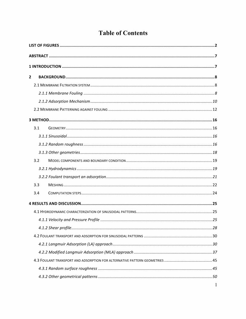
Table of Contents

LISTOFFIGURES...................................................................................................................................2

ABSTRACT............................................................................................................................................7

1INTRODUCTION.................................................................................................................................7

2 BACKGROUND..............................................................................................................................8

2.1MEMBRANEFILTRATIONSYSTEM...............................................................................................................8

2.1.1MembraneFouling.....................................................................................................................8

2.1.2AdsorptionMechanism.............................................................................................................10

2.2MEMBRANEPATTERNINGAGAINSTFOULING.............................................................................................12

3METHOD..........................................................................................................................................16

3.1 GEOMETRY...................................................................................................................................16

3.1.1Sinusoidal..................................................................................................................................16

3.1.2Randomroughness...................................................................................................................16

3.1.3Othergeometries......................................................................................................................18

3.2 MODELCOMPONENTSANDBOUNDARYCONDITION.............................................................................19

3.2.1Hydrodynamics.........................................................................................................................19

3.2.2Foulanttransportanadsorption...............................................................................................21

3.3 MESHING.....................................................................................................................................22

3.4 COMPUTATIONSTEPS.....................................................................................................................24

4RESULTSANDDISCUSSION...............................................................................................................25

4.1HYDRODYNAMICCHARACTERIZATIONOFSINUSOIDALPATTERNS....................................................................25

4.1.1VelocityandPressureProfile....................................................................................................25

4.1.2Shearprofile..............................................................................................................................28

4.2FOULANTTRANSPORTANDADSORPTIONFORSINUSOIDALPATTERNS.............................................................30

4.2.1LangmuirAdsorption(LA)approach.........................................................................................30

4.2.2ModifiedLangmuirAdsorption(MLA)approach......................................................................37

4.3FOULANTTRANSPORTANDADSORPTIONFORALTERNATIVEPATTERNGEOMETRIES...........................................45

4.3.1Randomsurfaceroughness......................................................................................................45

4.3.2Othergeometricalpatterns......................................................................................................50

2

5OTHEREFFORTS...............................................................................................................................55

5.1ADDITIONALSHEARTERM......................................................................................................................55

5.2ONESTEPSTUDY..................................................................................................................................55

6 FUTUREWORK...........................................................................................................................56

6.1PARTICLETRACING................................................................................................................................56

6.2TURBULENTMODELLING........................................................................................................................56

6.3EFFECTOFCONCENTRATIONPOLARIZATION...............................................................................................56

6.43DMODELING.....................................................................................................................................57

6 CONCLUSION..............................................................................................................................57

8REFERENCES....................................................................................................................................58

List of Abbreviations

CFD Computational Fluid Dynamics

UF Ultra-filtration

MF Micro-filtration

NF Nano-filtration

RO Reverse osmosis

OM Organic Matter

NOM Natural Organic Matter

BET Brunauer–Emmett–Teller

NIL Nano-Imprinting Lithography

BSA Bovine serum albumin

PES Polyethersulfone

3

List of Figures Figure 1 Schematic diagram of concentration polarization on membrane surface showing the

buildup gel layer (polarization layer) and boundary layer (Cheryan and Cheryan 1998). ... 10

Figure 2: Adsorption isotherms for Humic Acid (HA) adsorption on polyethersulfone membranes

(Demneh, Nasernejad, and Modarres 2011) ......................................................................... 11

Figure 3: (a) Schematic diagram of NIL process for membrane patterning by line and space silicon

mold, topographic AFM image of (b) non-patterned and (c) patterned membrane(Maruf,

Wang, et al. 2013) ................................................................................................................. 12

Figure 4: Permeate flux yield in different transmembrane pressure for imprinted (patterned) and

pristine (non-patterned) membrane both for DI water (no foulant) and colloidal (with silica

foulant) filtration (Maruf, Wang, et al. 2013). ...................................................................... 13

Figure 5: BSA adsorption isotherm for non-imprinted (non-patterned) and imprinted (patterned)

PES membrane (Maruf, Rickman, et al. 2013). .................................................................... 13

Figure 6 physical patterning on a membrane surface by deformation (Weinman and Husson 2016)

............................................................................................................................................... 14

Figure 7: simulated shear stress for (a) flat membrane and (b) prism patterned membrane and

confocal microscopy images of microbial (green) on membrane surfaces (red) in experiment:

(c) flat membrane and (d) prism patterned membrane. (Lee et al. 2013). ............................ 15

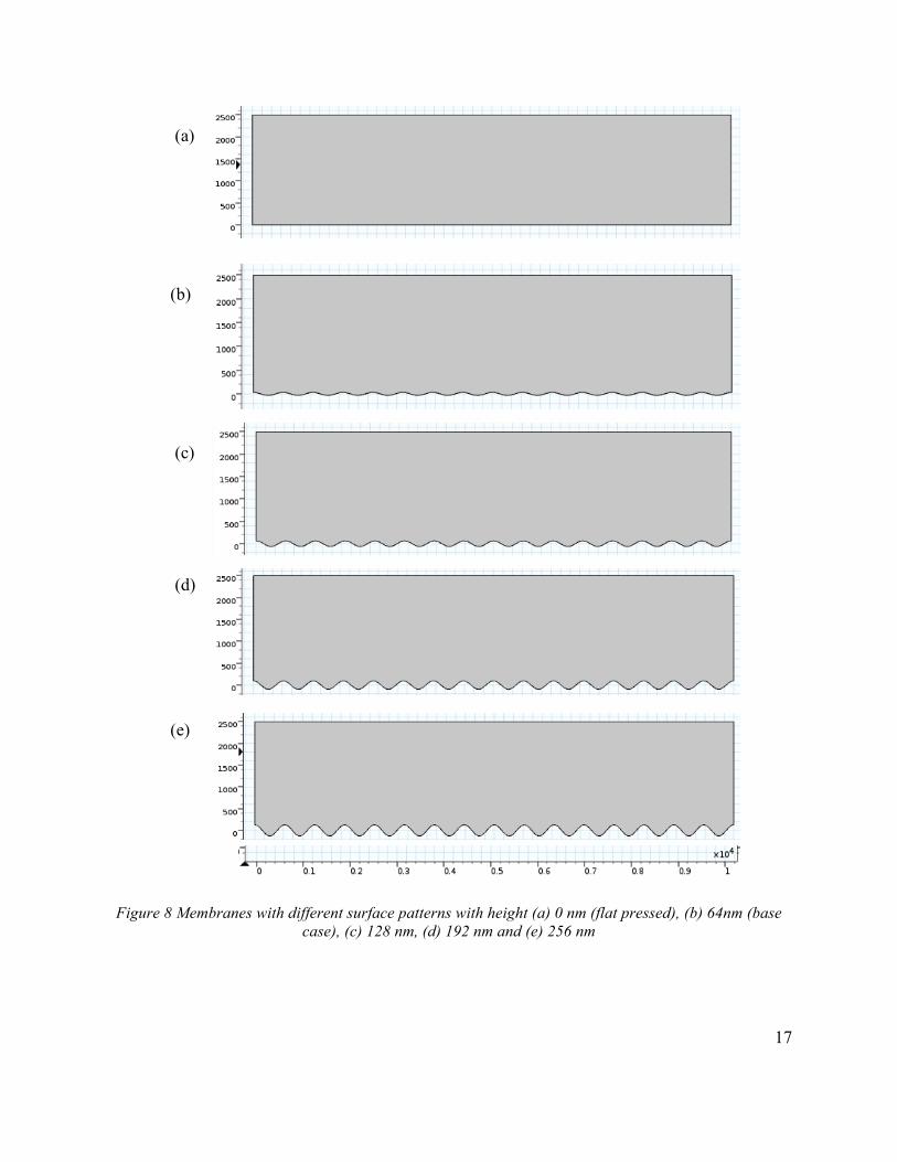
Figure 8 Membranes with different surface patterns with height (a) 0 nm (flat pressed), (b) 64nm

(base case), (c) 128 nm, (d) 192 nm and (e) 256 nm ............................................................ 17

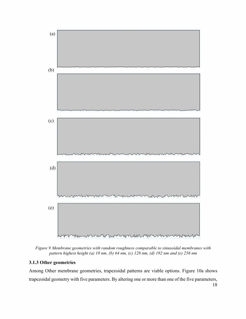
Figure 9 Membrane geometries with random roughness comparable to sinusoidal membranes with

pattern highest height (a) 10 nm, (b) 64 nm, (c) 128 nm, (d) 192 nm and (e) 256 nm ......... 18

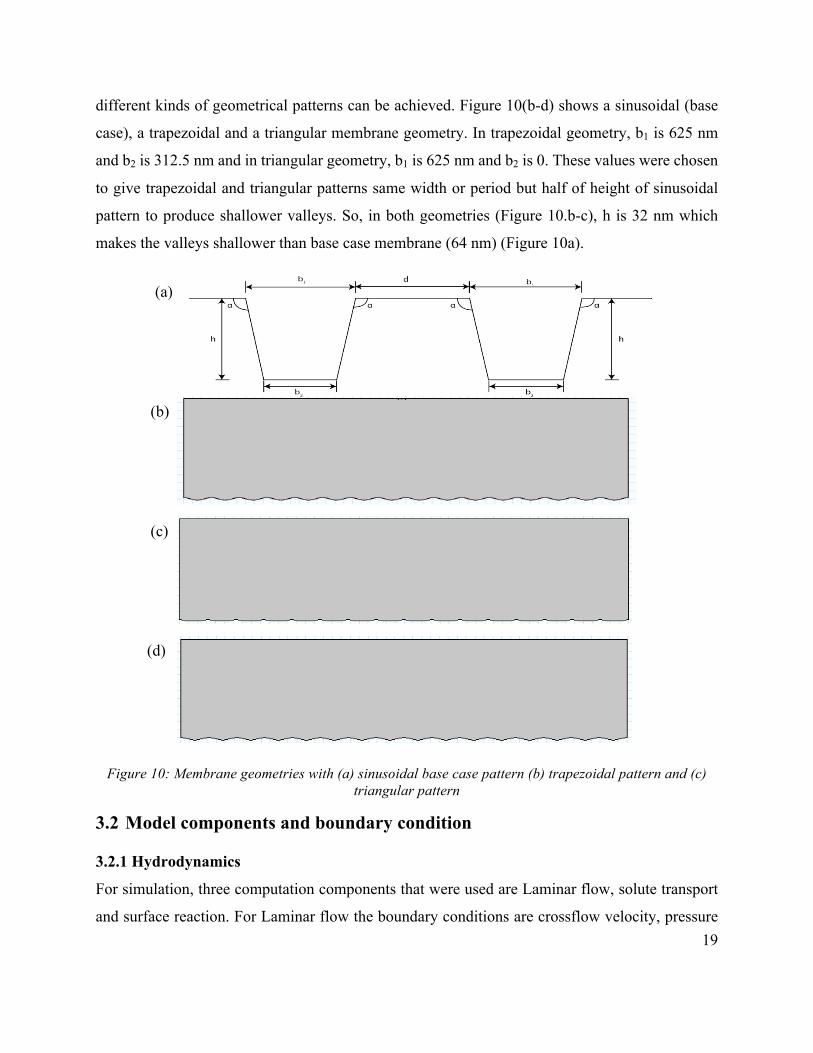
Figure 10: Membrane geometries with (a) sinusoidal base case pattern (b) trapezoidal pattern and

(c) triangular pattern ............................................................................................................. 19

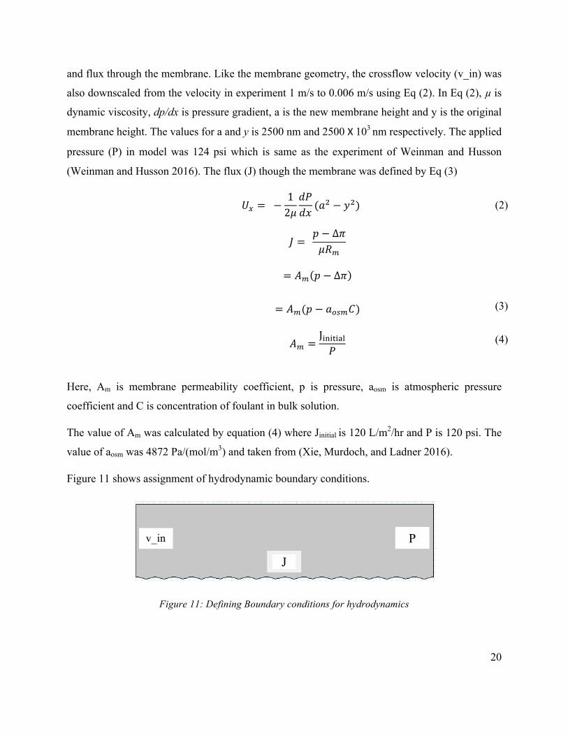
Figure 11: Defining Boundary conditions for hydrodynamics ..................................................... 20

Figure 12: Defining Boundary conditions for foulant transport and adsorption .......................... 21

4

Figure 13 2D modelling elements (Comsol 2016) ........................................................................ 22

Figure 13: Meshing of sinusoidal membranes with different pattern height (a) 0 nm (b) 64 nm, (c)

128 nm, (d) 192 nm and (e) 256 nm ..................................................................................... 23

Figure 15: Zoomed in view of Meshing of sinusoidal membranes with pattern height (a) 0 nm and

(b) .......................................................................................................................................... 24

Figure 16: Velocity magnitude profile of sinusoidal membranes with different pattern height (a) 0

nm (b) 64 nm, (c) 128 nm, (d) 192 nm and (e) 256 nm ........................................................ 26

Figure 17: Pressure profile of sinusoidal membranes with different pattern height (a)0 nm (b) 64

nm, (c) 128 nm, (d) 192 nm and (e) 256 nm ......................................................................... 27

Figure 18: Shear rate along the sinusoidal membrane surface with different pattern height ....... 28

Figure 19: shear rate profile of sinusoidal membranes with different pattern height (a) 0 nm, (b)

64 nm, (c) 128 nm, (d) 192 nm and (e) 256 nm .................................................................... 29

Figure 20: average foulant accumulation on membrane surface with time for five different

sinusoidal membranes. .......................................................................................................... 31

Figure 21 foulant accumulation on membrane surface for five different sinusoidal membranes on

a definite time point (120mins). ............................................................................................ 31

Figure 22: bulk concentration profiles at different time points of sinusoidal membranes with height

(a) 0 nm, (b) 64 nm and (c) 256 nm ...................................................................................... 32

Figure 23: Average flux through membrane over 24 hrs for sinusoidal membranes with different

pattern height. ....................................................................................................................... 33

Figure 24: (a) simulated and (b) experimental results for average flux through membrane over 120

mins (2hrs) for sinusoidal membrane geometries with different pattern height ................... 34

Figure 25: Change in flux decline trend in base case membranes with different (a)k1 and (b) k2

values for LA approach ......................................................................................................... 35

5

Figure 26: Change in flux decline trend in base case membrane with different F values for LA

approach ................................................................................................................................ 36

Figure 27: Effect of different inflow velocity on foulant accumulation on base case membrane

surface. .................................................................................................................................. 37

Figure 28: Foulant accumulation on membrane surface with effect of shear at a definite time point

(120mins) for sinusoidal membranes with different pattern heights. ................................... 38

Figure 29: Average foulant accumulation on membrane surface with effect of shear with time for

(a) 24 hrs (b) 2 hrs (120 mins) for sinusoidal membranes with different pattern heights. ... 39

Figure 30: Flux through membrane surface with effect of shear at a definite time point (120mins)

for sinusoidal membranes with different pattern heights. ..................................................... 41

Figure 31: Average flux through membrane with effect of shear with time for (a) 24 hrs (b) 2 hrs

(120 mins) for sinusoidal membranes with different pattern heights. .................................. 42

Figure 32: Change in flux decline trend with different (a)k1 and (b) k2 values for MLA Approach

............................................................................................................................................... 43

Figure 33: Accumulated foulnt on membrane surface after 120 mins for (a) k 1= 10-1 m3/mol/s, k2

= 10-6 (b) k1 = 10-3m3/mol/s, k2 = 10-6 ..................................................................................... 44

Figure 34: Change in flux decline trend with different F values in base case membrane for MLA

approach ................................................................................................................................ 45

Figure 35: shear profile of membrane geometries with random roughness comparable to sinusoidal

membranes with pattern height (a) 0 nm, (b) 64 nm, (c) 128 nm, (d) 192 nm and (e) 256 nm

............................................................................................................................................... 47

Figure 36: Average foulant accumulation on membrane surface with effect of shear with time for

(a) 24 hrs and (b) 120 mins for membranes with random roughness comparable to sinusoidal

membranes with pattern height 0 nm, 64 nm, 128 nm, 192 nm and 256 nm. ....................... 48

6

Figure 37: Average flux through membrane with effect of shear with time for (a) 24 hrs and (b)

120 mins for membranes with random roughness comparable to sinusoidal membranes with

pattern height 0 nm, 64 nm, 128 nm, 192 nm and 256 nm. .................................................. 49

Figure 38: Comparison of percentage of flux decline after 24 hrs for membranes with random

roughness to sinusoidal patterned membranes. ..................................................................... 50

Figure 39: Velocity profiles of membrane geometries with (a) sinusoidal pattern (64 nm) (b)

trapezoidal pattern and (c) triangular pattern. ....................................................................... 51

Figure 40: Shear profiles of membrane geometries with (a) sinusoidal pattern (64 nm) (b)

trapezoidal pattern and (c) triangular pattern. ....................................................................... 52

Figure 41: Comparison of shear on membrane surface of (a) sinusoidal and trapizoidal patterned

membrane and (b)sinusoidal and triangular patterned membrane ........................................ 53

Figure 42: Average flux through membrane with effect of shear with time (120 mins) for different

patterned membranes. ........................................................................................................... 54

Figure 43: Percentage of flux decline through membrane with effect of shear with time (120 mins)

for different patterned membranes ........................................................................................ 54

7

Abstract In this study, CFD simulations were conducted to demonstrate adsorption behavior of membranes

with modified surface. Langmuir Adsorption (LA) approach and Modified Langmuir Adsorption

(MLA) were used to simulate the adsorption process in membrane system with indirect and direct

effect of hydrodynamics respectively. The shear effect has been the key difference between these

two approaches. Simulation and comparative analysis for sinusoidal patterned membranes with

five different heights are presented here. LA approach was found mostly to depend on the

membrane surface area and MLA approach showed the direct effect of change in shear on foulant

adsorption for different membrane surface patterns. Membranes with random roughness,

trapezoidal and triangular patterns were also simulated using MLA approach and compared to

sinusoidal patterned membranes. Membranes with random roughness had more percentages of flux

decline than sinusoidal. But trapezoidal and triangular patterns were found to utilize the shear force

to have less flux decline and foulant accumulation compared to the sinusoidal pattern.

1 Introduction Membrane technology is one of the emerging innovations in water treatment and wastewater reuse.

Membranes yield treated water with high quality standards and are considered as reliable means

of treatment in wastewater treatment facilities (Singh 2006)(Zhang et al. 2013). Membrane

processes are typically integrated into a water treatment system like reverse osmosis (RO), nano-

filtration (NF), ultra-filtration (UF), micro-filtration (MF) (Šereš et al. 2016). RO and NF are

typically suitable for separation of small organics and electrolyte solutes(Bellona et al.

2004)(Verliefde et al. 2017) (Sayed 2010). These processes use hydrostatic pressure gradient and

osmotic pressure gradient as driving force (Ho and Sirkar 1992). The main limitation for RO and

NF is the permeate flux reduction and pressure drop which are caused by membrane fouling

(Vrouwenvelder et al. 2006)(Maruf, Wang, et al. 2013)(Maruf, Rickman, et al. 2013). Different

solutes like particles, colloids, salts, organic matters that come from biological wastewater

treatment system are highly probable to be adsorbed and accumulated on membrane surface which

eventually cause fouling (Xu et al. 2006a). Fouling can be minimized if the system is engineered

to prevent or minimize the adhesion of foulants onto membrane surface. The fouling propensity

8

varies depending on different types of feed water properties (A. Al-Amoudi and Lovitt 2007)

(Zhang et al. 2013)(Singh 2006).

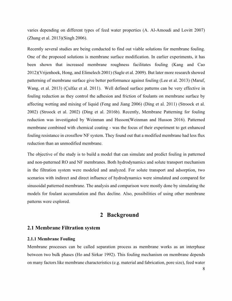
Recently several studies are being conducted to find out viable solutions for membrane fouling.

One of the proposed solutions is membrane surface modification. In earlier experiments, it has

been shown that increased membrane roughness facilitates fouling (Kang and Cao

2012)(Vrijenhoek, Hong, and Elimelech 2001) (Sagle et al. 2009). But later more research showed

patterning of membrane surface give better performance against fouling (Lee et al. 2013) (Maruf,

Wang, et al. 2013) (Çulfaz et al. 2011). Well defined surface patterns can be very effective in

fouling reduction as they control the adhesion and friction of foulants on membrane surface by

affecting wetting and mixing of liquid (Feng and Jiang 2006) (Ding et al. 2011) (Stroock et al.

2002) (Stroock et al. 2002) (Ding et al. 2016b). Recently, Membrane Patterning for fouling

reduction was investigated by Weinman and Husson(Weinman and Husson 2016). Patterned

membrane combined with chemical coating - was the focus of their experiment to get enhanced

fouling resistance in crossflow NF system. They found out that a modified membrane had less flux

reduction than an unmodified membrane.

The objective of the study is to build a model that can simulate and predict fouling in patterned

and non-patterned RO and NF membranes. Both hydrodynamics and solute transport mechanism

in the filtration system were modeled and analyzed. For solute transport and adsorption, two

scenarios with indirect and direct influence of hydrodynamics were simulated and compared for

sinusoidal patterned membrane. The analysis and comparison were mostly done by simulating the

models for foulant accumulation and flux decline. Also, possibilities of using other membrane

patterns were explored.

2 Background

2.1 Membrane Filtration system

2.1.1 Membrane Fouling

Membrane processes can be called separation process as membrane works as an interphase

between two bulk phases (Ho and Sirkar 1992). This fouling mechanism on membrane depends

on many factors like membrane characteristics (e.g. material and fabrication, pore size), feed water

9

characteristics (e.g. solute loading, solute size distribution), hydraulic conditions, operating

conditions etc. (Singh 2006)(Zhang et al. 2013). Membrane fouling has four different types: (a)

Deposition – from silt and suspended solids, (b) Scaling - form inorganic deposits from soluble

salts (c) Biofouling - from microbial growth and (d) organic fouling – from natural or synthetic

organics(Kao et al. 2012). Among the membrane foulants, the most important is organic matter

(OM) in NF and RO filtration system (A. S. Al-Amoudi 2010). A range of soluble organic

compounds present in biologically treated wastewater constitutes the OM. OM can be classified

into three classes: (a) Natural Organic Matter (NOM) (b) Synthetic Organic matter (c) Soluble

microbial products (Drewes and Fox 1999). NOMs are found to be most active in causing

membrane fouling (Xu et al. 2006b). Hydrophobicity of NF Membranes and roughness of RO

membranes increases after the adsorption of NOM (Yongki Shim et al. 2002) and protein

adsorption (Bowen, Doneva, and Yin 2002) respectively. Due to fouling, Changes in membrane

surface characteristics like membrane hydrophobicity, surface charge and surface morphology

causes change in membrane performance (Xu et al. 2006b). Pore blocking, concentration

polarization and cake formation leads to the reduction of permeate flux and increased flow

resistance (Lim and Bai 2003)(Jarusutthirak, Amy, and Croué 2002). Long term fouling can lead

to irreversible fouling from microbial action and reduction of membrane lifetime (Lim and Bai

2003).

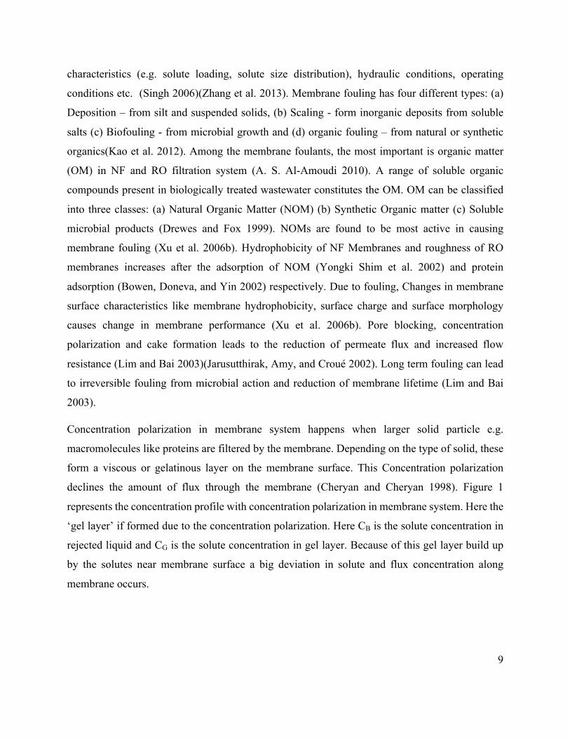
Concentration polarization in membrane system happens when larger solid particle e.g.

macromolecules like proteins are filtered by the membrane. Depending on the type of solid, these

form a viscous or gelatinous layer on the membrane surface. This Concentration polarization

declines the amount of flux through the membrane (Cheryan and Cheryan 1998). Figure 1

represents the concentration profile with concentration polarization in membrane system. Here the

‘gel layer’ if formed due to the concentration polarization. Here CB is the solute concentration in

rejected liquid and CG is the solute concentration in gel layer. Because of this gel layer build up

by the solutes near membrane surface a big deviation in solute and flux concentration along

membrane occurs.

10

Figure 1 Schematic diagram of concentration polarization on membrane surface showing the buildup gel layer (polarization layer) and boundary layer (Cheryan and Cheryan 1998).

2.1.2 Adsorption Mechanism

In liquid-solid systems, Langmuir, BET and Freundlich isotherms are usually very convenient for

environmental modeling, explanation of experimental data and designing equipment (Clark 2009).

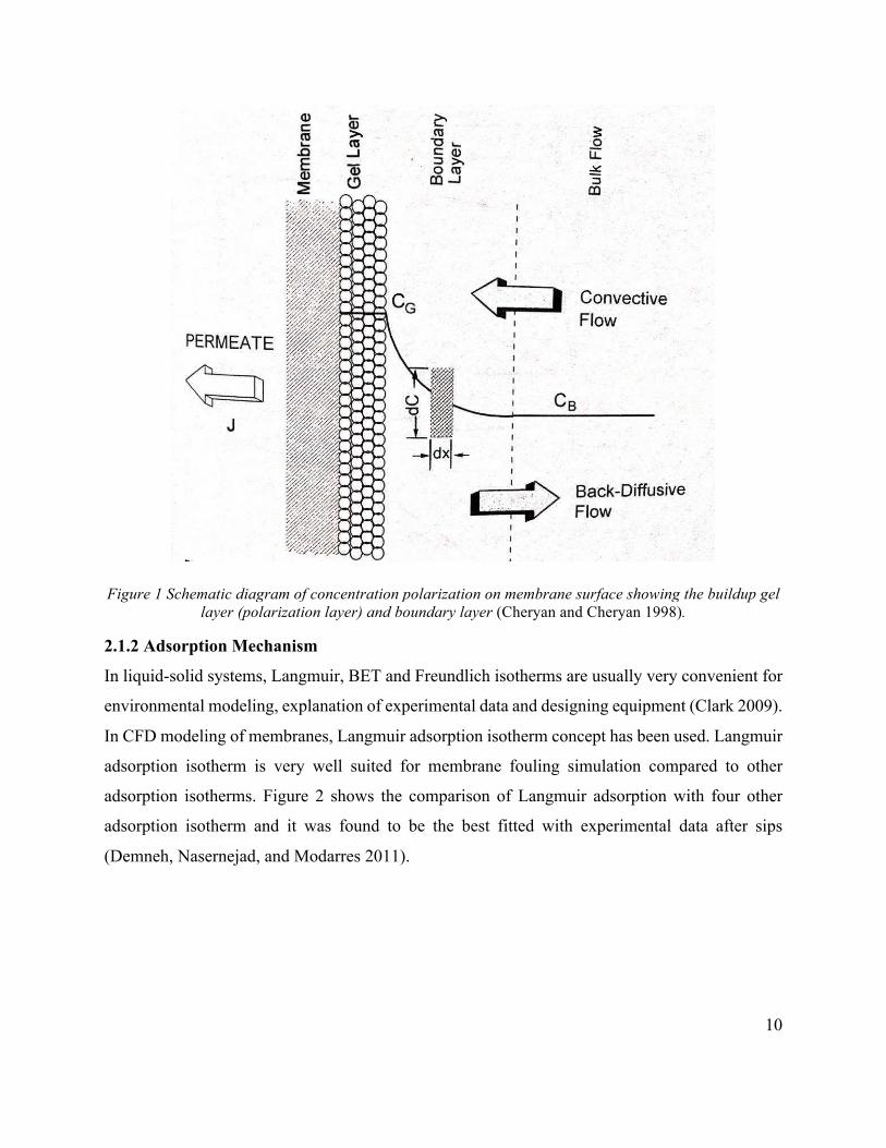
In CFD modeling of membranes, Langmuir adsorption isotherm concept has been used. Langmuir

adsorption isotherm is very well suited for membrane fouling simulation compared to other

adsorption isotherms. Figure 2 shows the comparison of Langmuir adsorption with four other

adsorption isotherm and it was found to be the best fitted with experimental data after sips

(Demneh, Nasernejad, and Modarres 2011).

11

Figure 2: Adsorption isotherms for Humic Acid (HA) adsorption on polyethersulfone membranes (Demneh, Nasernejad, and Modarres 2011)

According to Langmuir isotherm, it is assumed that the rate of desorption is proportional to the

amount of solute that occupies the surface (Clark 2009). So,

Rate of desorption = 𝐾"𝐶$

Here, K2 is desorption coefficient and Cs is accumulated solute on solid surface.

Hence, the rate of adsorption is proportional to the difference between the concentration of solute

at equilibrium and the concentration of accumulated solute on the solid surface. So,

Rate of adsorption = 𝐾&𝐶(𝐶$( − 𝐶$)

Here, K1 is adsorption coefficient, C is concentration of solute in solution and Cse is the

concentration of accumulated solute on solid surface at equilibrium. So, the change in

concentration of accumulated solute on solid surface can be written as following (Clark 2009):

𝑑𝐶$𝑑𝑡 = 𝐾&𝐶 𝐶$( − 𝐶$ −𝐾"𝐶$ (1)

In Equation 1, any definite the unit of k1 and k2 has not been found so far. (Jones and O’Melia

2000) reported calculation of k1 and k2 in his work. Although the units don’t agree with equation

(1) and don’t give the same unit for each term of the equation.

12

2.2 Membrane Patterning against fouling

Surface patterning is one of the latest trends in the area of physical modification of membrane to

reduce fouling. For fouling reduction, two surface modification methods that have been mostly

used so far are phase separation micro-molding (Çulfaz et al. 2011)(Laura Vogelaar et al. 2005)(L.

Vogelaar et al. 2003)(Gironès et al. 2006)(Bikel et al. 2009) and thermal embossing NIL

(Nanoimprint Lithography) process(Wang and Ding 2010)(Chou 1996)(Guo 2007). In phase

inversion process, polymer solutions of the membrane are kept in structured molds to solidify and

become patterned (Laura Vogelaar et al. 2005). In NIL process, a viscous polymer film is pressed

by a nanostructured mold in certain temperature and force (thermal embossing) (Chou

1996)(Weinman and Husson 2016).

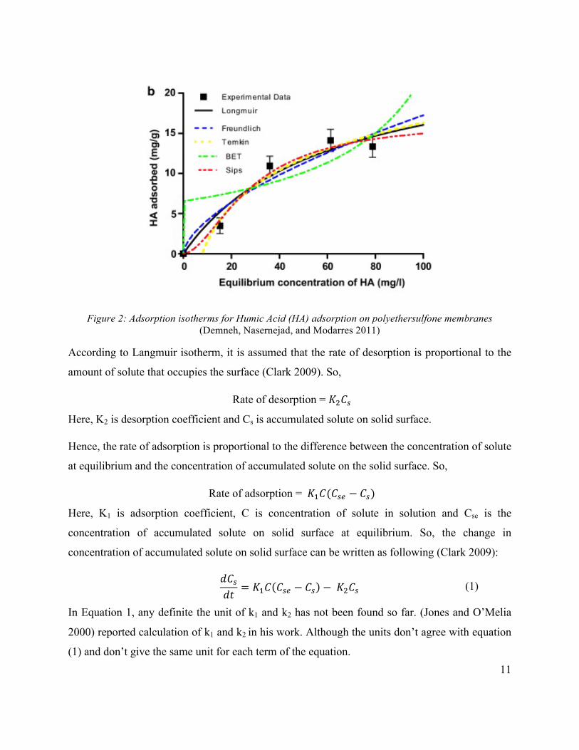
The first direct and effective NIL patterning on membrane was reported by (Maruf, Wang, et al.

2013). They used commercial polyethersulfone UF-type membrane and used a silicon mold which

had line and spaces with 1:1 ratio. The patterning process was done in 120°C with a pressure of

4MPa for 180s. The patterning process is illustrated in Figure 3a. Figure 3b and Figure 3c shows

the change in membrane topographic vertical dimension before and after patterning.

Figure 3: (a) Schematic diagram of NIL process for membrane patterning by line and space silicon mold, topographic AFM image of (b) non-patterned and (c) patterned membrane(Maruf, Wang, et al. 2013)

13

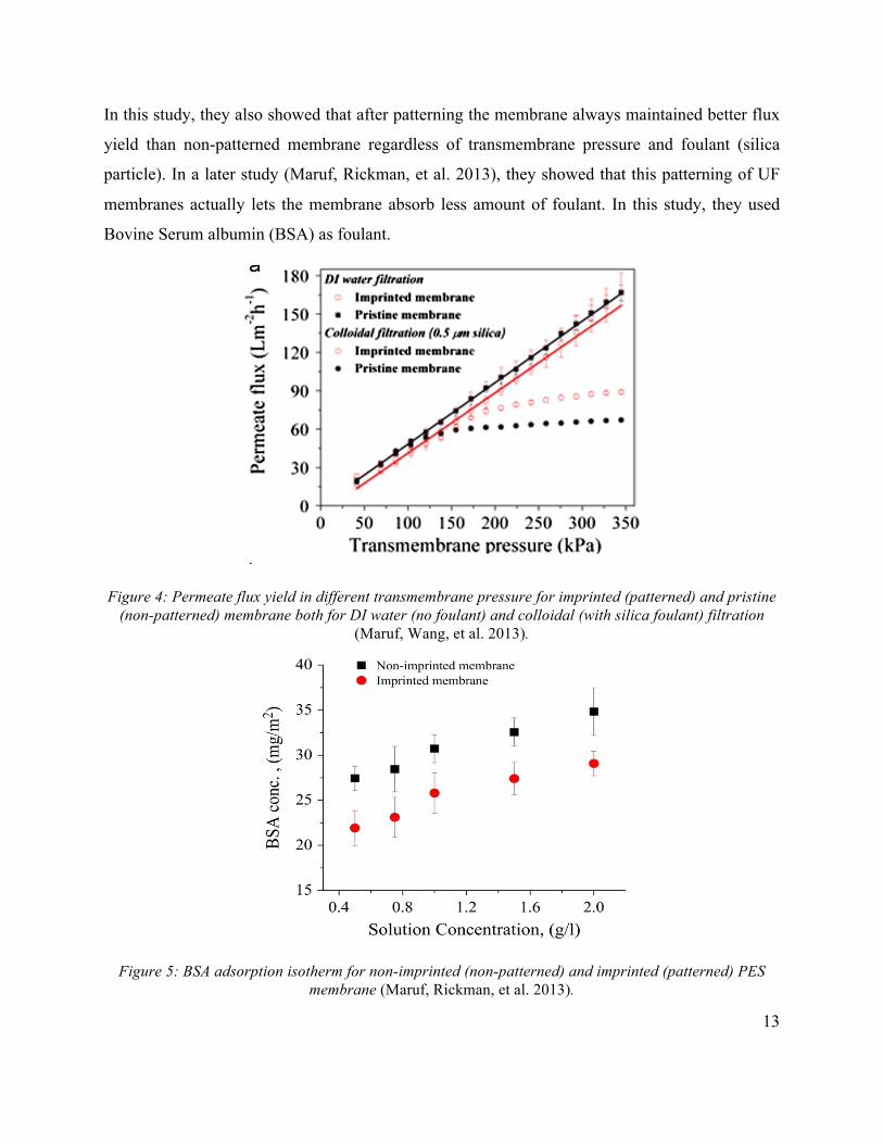
In this study, they also showed that after patterning the membrane always maintained better flux

yield than non-patterned membrane regardless of transmembrane pressure and foulant (silica

particle). In a later study (Maruf, Rickman, et al. 2013), they showed that this patterning of UF

membranes actually lets the membrane absorb less amount of foulant. In this study, they used

Bovine Serum albumin (BSA) as foulant.

Figure 4: Permeate flux yield in different transmembrane pressure for imprinted (patterned) and pristine (non-patterned) membrane both for DI water (no foulant) and colloidal (with silica foulant) filtration

(Maruf, Wang, et al. 2013).

Figure 5: BSA adsorption isotherm for non-imprinted (non-patterned) and imprinted (patterned) PES membrane (Maruf, Rickman, et al. 2013).

14

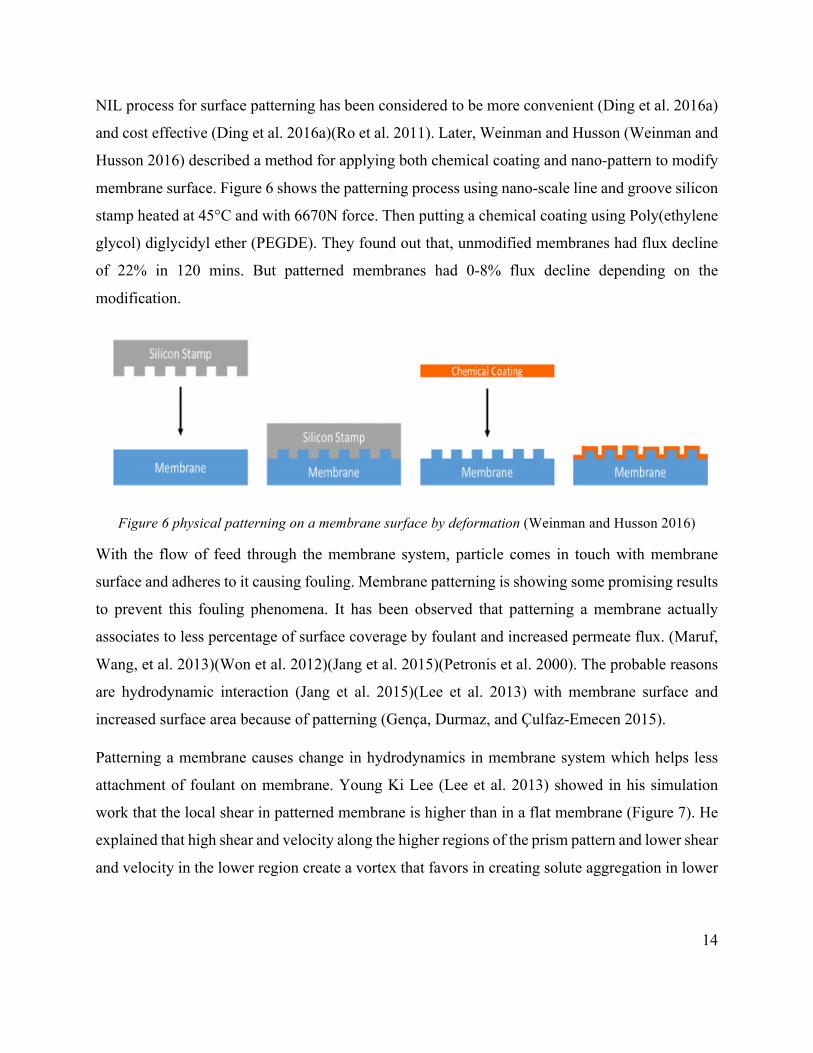
NIL process for surface patterning has been considered to be more convenient (Ding et al. 2016a)

and cost effective (Ding et al. 2016a)(Ro et al. 2011). Later, Weinman and Husson (Weinman and

Husson 2016) described a method for applying both chemical coating and nano-pattern to modify

membrane surface. Figure 6 shows the patterning process using nano-scale line and groove silicon

stamp heated at 45°C and with 6670N force. Then putting a chemical coating using Poly(ethylene

glycol) diglycidyl ether (PEGDE). They found out that, unmodified membranes had flux decline

of 22% in 120 mins. But patterned membranes had 0-8% flux decline depending on the

modification.

Figure 6 physical patterning on a membrane surface by deformation (Weinman and Husson 2016)

With the flow of feed through the membrane system, particle comes in touch with membrane

surface and adheres to it causing fouling. Membrane patterning is showing some promising results

to prevent this fouling phenomena. It has been observed that patterning a membrane actually

associates to less percentage of surface coverage by foulant and increased permeate flux. (Maruf,

Wang, et al. 2013)(Won et al. 2012)(Jang et al. 2015)(Petronis et al. 2000). The probable reasons

are hydrodynamic interaction (Jang et al. 2015)(Lee et al. 2013) with membrane surface and

increased surface area because of patterning (Gença, Durmaz, and Çulfaz-Emecen 2015).

Patterning a membrane causes change in hydrodynamics in membrane system which helps less

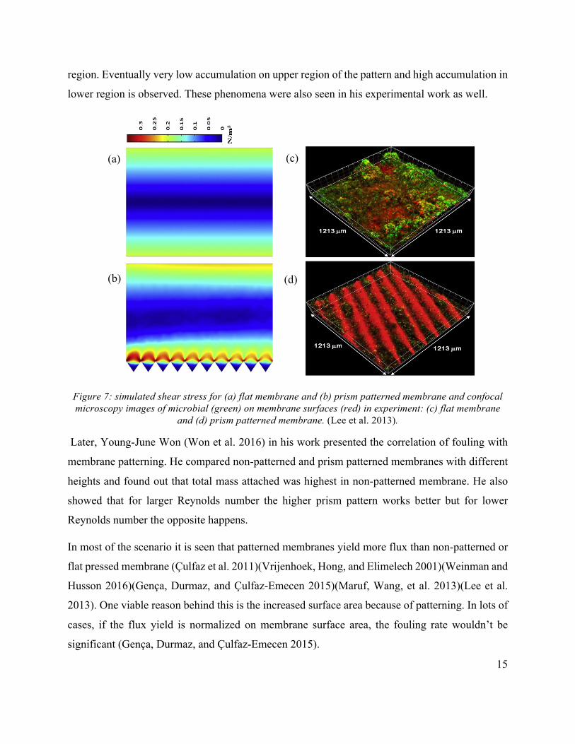
attachment of foulant on membrane. Young Ki Lee (Lee et al. 2013) showed in his simulation

work that the local shear in patterned membrane is higher than in a flat membrane (Figure 7). He

explained that high shear and velocity along the higher regions of the prism pattern and lower shear

and velocity in the lower region create a vortex that favors in creating solute aggregation in lower

15

region. Eventually very low accumulation on upper region of the pattern and high accumulation in

lower region is observed. These phenomena were also seen in his experimental work as well.

Figure 7: simulated shear stress for (a) flat membrane and (b) prism patterned membrane and confocal microscopy images of microbial (green) on membrane surfaces (red) in experiment: (c) flat membrane

and (d) prism patterned membrane. (Lee et al. 2013).

Later, Young-June Won (Won et al. 2016) in his work presented the correlation of fouling with

membrane patterning. He compared non-patterned and prism patterned membranes with different

heights and found out that total mass attached was highest in non-patterned membrane. He also

showed that for larger Reynolds number the higher prism pattern works better but for lower

Reynolds number the opposite happens.

In most of the scenario it is seen that patterned membranes yield more flux than non-patterned or

flat pressed membrane (Çulfaz et al. 2011)(Vrijenhoek, Hong, and Elimelech 2001)(Weinman and

Husson 2016)(Gença, Durmaz, and Çulfaz-Emecen 2015)(Maruf, Wang, et al. 2013)(Lee et al.

2013). One viable reason behind this is the increased surface area because of patterning. In lots of

cases, if the flux yield is normalized on membrane surface area, the fouling rate wouldn’t be

significant (Gença, Durmaz, and Çulfaz-Emecen 2015).

(a)

(b)

(c)

(d)

16

3 Method For this study, simulation of flow behavior and fouling on membrane surface was done in Comsol

Multiphysics 5.2. The geometry properties of sinusoidal membranes and inflow characteristics

were taken from Weinman and Husson’s work (Weinman and Husson 2016).

3.1 Geometry

In this study, 2D CFD models were constructed to simulate the membrane performance with

different pattern geometries.

3.1.1 Sinusoidal

The membrane cross section that was used in the experiment of Weinman and husson (2016) was

1 cm × 2.5 mm. The pattern on the membrane was a sinusoidal pattern with amplitude of 32 nm

(64 nm pattern height) and period 625 nm. For modelling, the membrane cross section was

downscaled by 1000 keeping the membrane pattern same. Therefore, the developed model was a

very small portion of the original membrane cross section in experiment. Figure 8 shows the

membrane geometry in model that represents the flat pressed with 0 nm pattern height (Figure 8a)

and ‘base case’ patterned (Figure 8b) membrane with pattern height 64nm in (Weinman and

Husson 2016)’s work. Here, pattern height indicates the distance from lowest point of a valley to

highest point of a peak of sinusoidal geometry. For better comparison, 3 additional sinusoidal

patterned membranes were simulated with same period 625 nm but different pattern height 128

nm, 192 nm and 256 nm (Figure 8(c-e)).

3.1.2 Random roughness

When a membrane is not patterned or pressed, it has random surface roughness. To explore

adsorption mechanism of membranes with random roughness and make a comparison with

sinusoidal patterned membranes, five different membrane geometries with random surface

roughness were constructed and analyzed. Five random geometries are presented in Figure 9 with

highest pattern height (height from peak to valley) of 10nm, 64 nm, 128 nm, 192 nm and 256 nm

comparable to sinusoidal membranes with pattern height of 0nm, 64 nm, 128 nm, 192 nm and 256

nm respectively.

17

Figure 8 Membranes with different surface patterns with height (a) 0 nm (flat pressed), (b) 64nm (base case), (c) 128 nm, (d) 192 nm and (e) 256 nm

(a)

(d)

(c)

(b)

(e)

18

Figure 9 Membrane geometries with random roughness comparable to sinusoidal membranes with pattern highest height (a) 10 nm, (b) 64 nm, (c) 128 nm, (d) 192 nm and (e) 256 nm

3.1.3 Other geometries

Among Other membrane geometries, trapezoidal patterns are viable options. Figure 10a shows

trapezoidal geometry with five parameters. By altering one or more than one of the five parameters,

(a)

(b)

(c)

(d)

(e)

19

different kinds of geometrical patterns can be achieved. Figure 10(b-d) shows a sinusoidal (base

case), a trapezoidal and a triangular membrane geometry. In trapezoidal geometry, b1 is 625 nm

and b2 is 312.5 nm and in triangular geometry, b1 is 625 nm and b2 is 0. These values were chosen

to give trapezoidal and triangular patterns same width or period but half of height of sinusoidal

pattern to produce shallower valleys. So, in both geometries (Figure 10.b-c), h is 32 nm which

makes the valleys shallower than base case membrane (64 nm) (Figure 10a).

Figure 10: Membrane geometries with (a) sinusoidal base case pattern (b) trapezoidal pattern and (c) triangular pattern

3.2 Model components and boundary condition

3.2.1 Hydrodynamics

For simulation, three computation components that were used are Laminar flow, solute transport

and surface reaction. For Laminar flow the boundary conditions are crossflow velocity, pressure

(a)

(b)

(c)

(d)

20

and flux through the membrane. Like the membrane geometry, the crossflow velocity (v_in) was

also downscaled from the velocity in experiment 1 m/s to 0.006 m/s using Eq (2). In Eq (2), µ is

dynamic viscosity, dp/dx is pressure gradient, a is the new membrane height and y is the original

membrane height. The values for a and y is 2500 nm and 2500 X103 nm respectively. The applied

pressure (P) in model was 124 psi which is same as the experiment of Weinman and Husson

(Weinman and Husson 2016). The flux (J) though the membrane was defined by Eq (3)

𝑈/ = −12𝜇𝑑𝑃𝑑𝑥 (𝑎

" − 𝑦") (2)

𝐽 = 𝑝 − ∆𝜋𝜇𝑅<

= 𝐴< 𝑝 − ∆𝜋

= 𝐴<(𝑝 − 𝑎>$<𝐶) (3)

𝐴< =J@A@B@CD𝑃 (4)

Here, Am is membrane permeability coefficient, p is pressure, aosm is atmospheric pressure

coefficient and C is concentration of foulant in bulk solution.

The value of Am was calculated by equation (4) where Jinitial is 120 L/m2/hr and P is 120 psi. The

value of aosm was 4872 Pa/(mol/m3) and taken from (Xie, Murdoch, and Ladner 2016).

Figure 11 shows assignment of hydrodynamic boundary conditions.

Figure 11: Defining Boundary conditions for hydrodynamics

J

v_in P

21

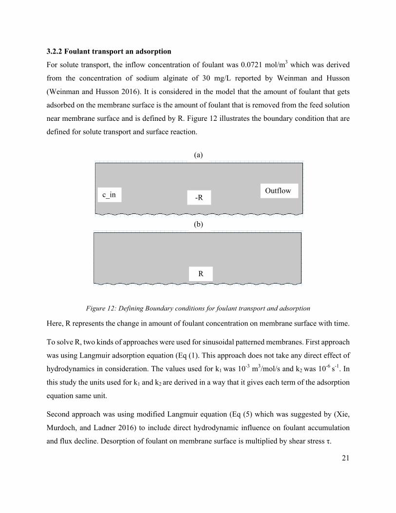
3.2.2 Foulant transport an adsorption

For solute transport, the inflow concentration of foulant was 0.0721 mol/m3 which was derived

from the concentration of sodium alginate of 30 mg/L reported by Weinman and Husson

(Weinman and Husson 2016). It is considered in the model that the amount of foulant that gets

adsorbed on the membrane surface is the amount of foulant that is removed from the feed solution

near membrane surface and is defined by R. Figure 12 illustrates the boundary condition that are

defined for solute transport and surface reaction.

Figure 12: Defining Boundary conditions for foulant transport and adsorption

Here, R represents the change in amount of foulant concentration on membrane surface with time.

To solve R, two kinds of approaches were used for sinusoidal patterned membranes. First approach

was using Langmuir adsorption equation (Eq (1). This approach does not take any direct effect of

hydrodynamics in consideration. The values used for k1 was 10-3 m3/mol/s and k2 was 10-6 s-1. In

this study the units used for k1 and k2 are derived in a way that it gives each term of the adsorption

equation same unit.

Second approach was using modified Langmuir equation (Eq (5) which was suggested by (Xie,

Murdoch, and Ladner 2016) to include direct hydrodynamic influence on foulant accumulation

and flux decline. Desorption of foulant on membrane surface is multiplied by shear stress τ.

Outflow -R

(a)

(b)

c_in

R

22

𝑑𝐶$𝑑𝑡 = 𝐾&𝐶 𝐶$( − 𝐶$ −𝐾"𝐶$𝜏 (5)

Here, foulant concentration in equlibrium, Cse was 1 mol/m2 for both approaches. The values and

units for k1 and k2 were changed. The value of k1 was 10-1 m3/mol/s and k2 was 10-6 s-2.

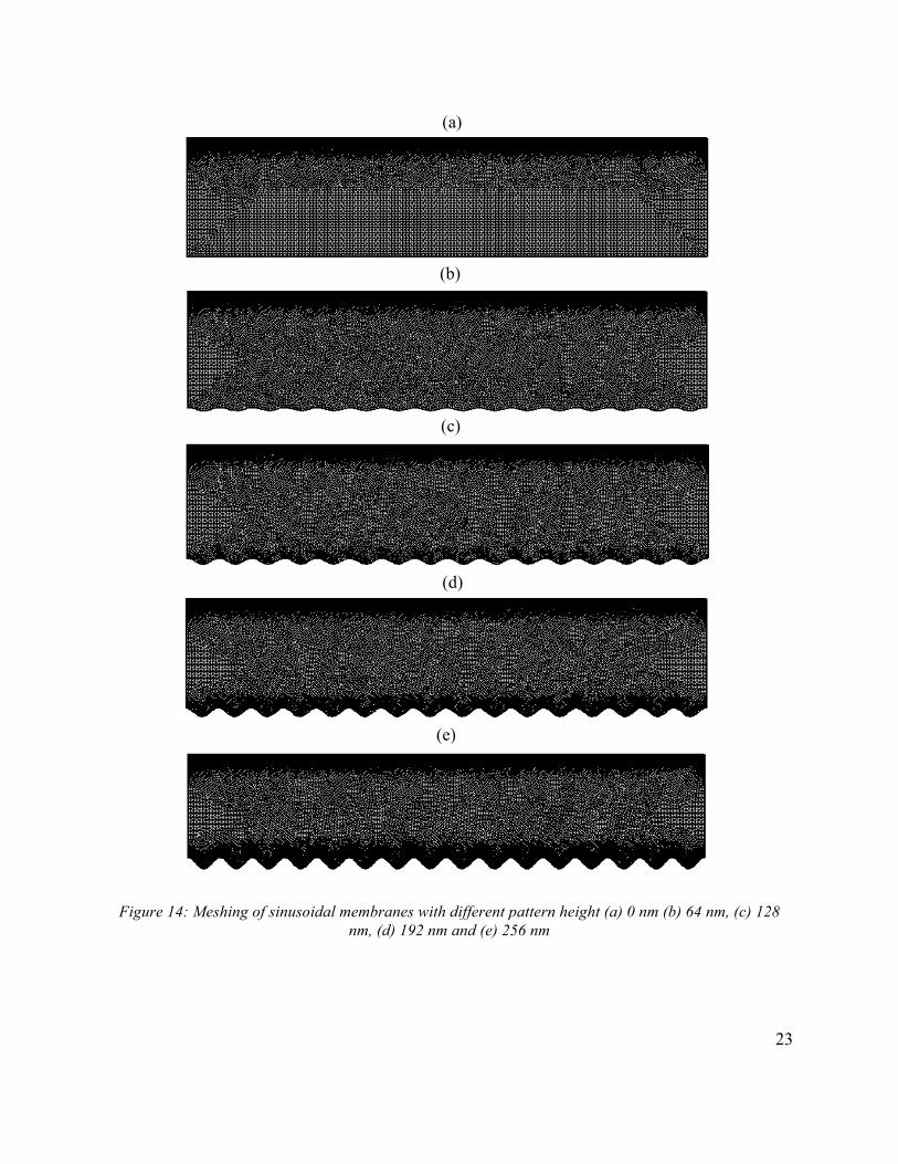
3.3 Meshing

The purpose of meshing is to subdivide geometry into ‘elements’ for modelling and used to solve

and represent the solution field of the problems (Frei 2013). For 2D modelling, triangular and

quadrilateral (Figure 13) elements and for 3D modelling, tetrahedra, hexahedra, triangular

prismatics and pyramid elements are available (Frei 2013). In Figure 13 the black circles are the

corners, or ‘nodes’. For this study, Physics controlled meshing was done using triangular elements

for 2D models which is inbuilt meshing in COMSOL. For membranes with different geometries

constitutes different number of domain elements. The meshing for 5 geometries are presented in

Figure 14. As, the same type of physics controlled meshing was used for all membranes.

In the zoomed in version of meshing, for flat pressed membrane (Figure 15a) the meshing is

uniform all over membrane geometry. But for patterned membrane (Figure 15b) the mesh element

size and number varied depending on the change in membrane pattern. When the patterned

geometry changes, the models require more mesh elements to make accurate calculations.

Figure 13 2D modelling elements (Comsol 2016)

23

Figure 14: Meshing of sinusoidal membranes with different pattern height (a) 0 nm (b) 64 nm, (c) 128 nm, (d) 192 nm and (e) 256 nm

(a) (a)

(b)

(c)

(d)

(e)

24

Figure 15: Zoomed in view of Meshing of sinusoidal membranes with pattern height (a) 0 nm and (b)

3.4 Computation steps

Two step calculation was done for the simulation. In first step, laminar flow modeling was done

in steady state condition. In this step, velocity, pressure and shear was calculated. Next, in time

dependent step, the solute transport and surface reaction modeling was done using the results from

steady state step. Time dependent step calculates change in foulant concentration in bulk solution

and on membrane surface. Time dependent calculation was done for 24 hrs for both simulation

approach.

(a) (b)

25

4 Results and Discussion

4.1 Hydrodynamic characterization of sinusoidal patterns

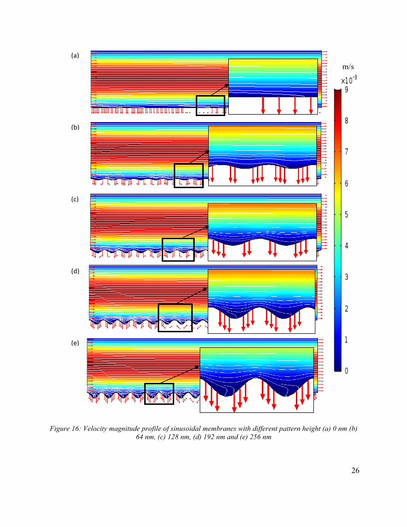
4.1.1 Velocity and Pressure Profile

The laminar flow velocity profiles that are generated in steady state step are presented in Figure

16. The white lines represent streamlines through the membrane cross section and red arrows show

the fluid flux entrance and exit direction. In all five membranes, the velocity was highest in the

center. The zoomed in view of the velocity profiles in Figure 16(a-e) illustrates that stream flows

are different among different membrane patterns. The flat pressed membrane had straight stream

lines near membrane surface, where 64nm pattern makes the streamlines curved along the

membrane surface. In the 256 nm pattern (Figure 16.e), the curved streamlines are more prominent.

These different streamline deviations show how the hydrodynamics can be different in different

membrane patterns and can have different effects on foulant accumulation. In higher pattern

height, the curvature of streamlines are higher which produce more shear stress on the peaks of

the patterns. Also, if the pattern height is big enough, the water flow tends to create full vortex

which in some extent facilitates foulant aggregation. In Figure 16(e), the curved streamlines in the

valleys show initiation of a vortex.

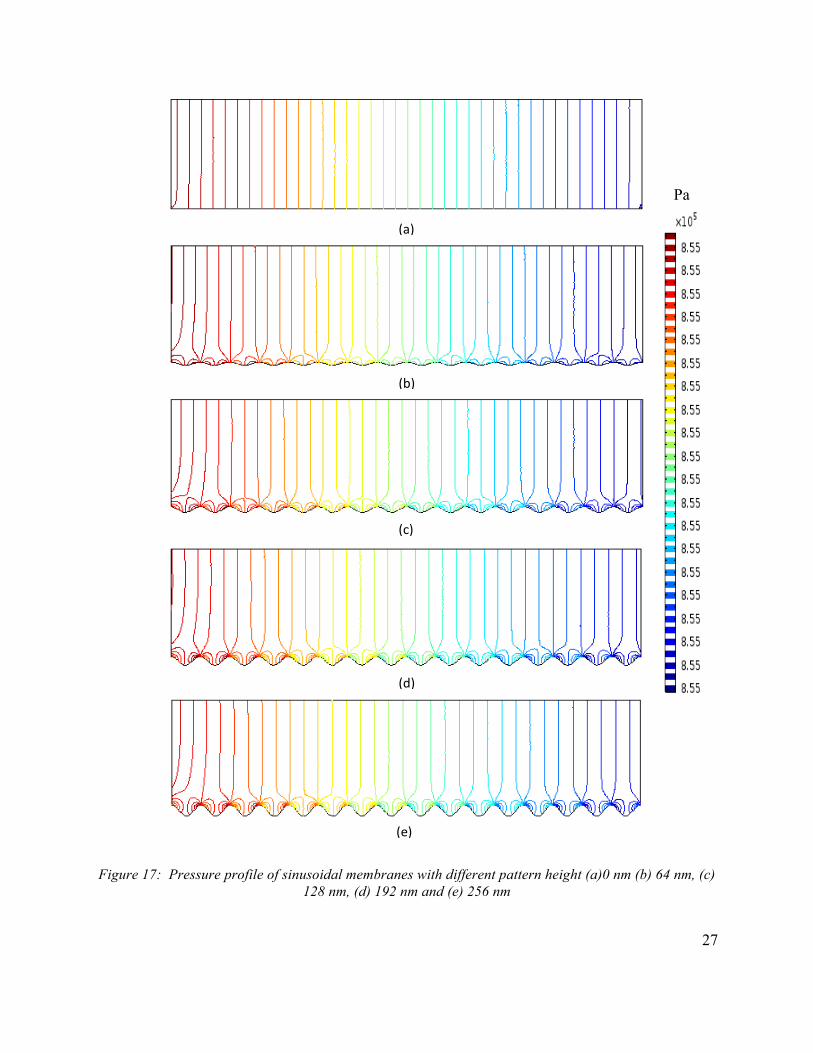
The pressure profiles in Figure 17 represent the pressure change in the membrane as the feed water

flows from left to right and through the membrane surface maintaining a fixed flux in steady state.

When a membrane is patterned, a difference in pressure can be seen between left and right side of

the pattern peak. With increase in pattern height the difference becomes higher. This also gives an

indication of change in effect of hydrodynamics with change in membrane pattern.

26

Figure 16: Velocity magnitude profile of sinusoidal membranes with different pattern height (a) 0 nm (b) 64 nm, (c) 128 nm, (d) 192 nm and (e) 256 nm

(a)

(b)

(c)

(d)

(e)

m/s

27

Figure 17: Pressure profile of sinusoidal membranes with different pattern height (a)0 nm (b) 64 nm, (c) 128 nm, (d) 192 nm and (e) 256 nm

(a)

(b)

(c)

(d)

(e)

Pa

28

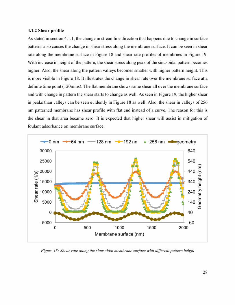
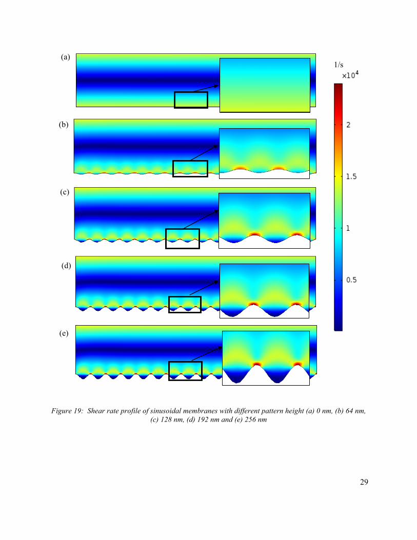
4.1.2 Shear profile

As stated in section 4.1.1, the change in streamline direction that happens due to change in surface

patterns also causes the change in shear stress along the membrane surface. It can be seen in shear

rate along the membrane surface in Figure 18 and shear rate profiles of membrnes in Figure 19.

With increase in height of the pattern, the shear stress along peak of the sinusoidal pattern becomes

higher. Also, the shear along the pattern valleys becomes smaller with higher pattern height. This

is more visible in Figure 18. It illustrates the change in shear rate over the membrane surface at a

definite time point (120mins). The flat membrane shows same shear all over the membrane surface

and with change in pattern the shear starts to change as well. As seen in Figure 19, the higher shear

in peaks than valleys can be seen evidently in Figure 18 as well. Also, the shear in valleys of 256

nm patterned membrane has shear profile with flat end instead of a curve. The reason for this is

the shear in that area became zero. It is expected that higher shear will assist in mitigation of

foulant adsorbance on membrane surface.

Figure 18: Shear rate along the sinusoidal membrane surface with different pattern height

-60

40

140

240

340

440

540

640

-5000

0

5000

10000

15000

20000

25000

30000

0 500 1000 1500 2000

Geo

met

ry h

eigh

t (nm

)

Shea

r rat

e (1

/s)

Membrane surface (nm)

0 nm 64 nm 128 nm 192 nn 256 nm geometry

29

Figure 19: Shear rate profile of sinusoidal membranes with different pattern height (a) 0 nm, (b) 64 nm, (c) 128 nm, (d) 192 nm and (e) 256 nm

(a)

(b)

(c)

(d)

(e)

1/s

30

4.2 Foulant transport and adsorption for sinusoidal patterns

4.2.1 Langmuir Adsorption (LA) approach

While water passing through, foulant accumulates due to the adsorption on membrane surface. To

calculate foulant transport and adsorption, the first approach was using Langmuir adsorption

equation (1).

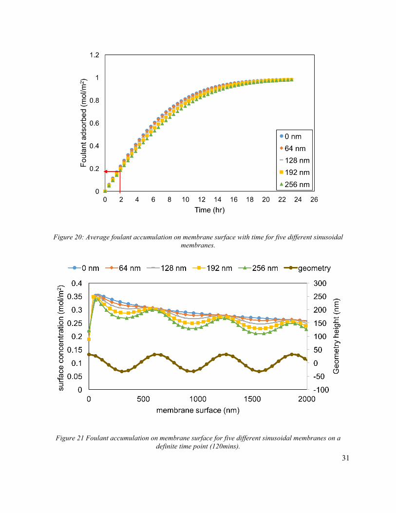
4.2.1.1 Foulant accumulation on membrane surface

In the model, adsorption and desorption in membrane filtration process happens simultaneously

until it reaches the equilibrium surface concentration (Cse) with time. The adsorption (k1) and

desorption (k2) coefficients play an important role to control the time that the system takes to reach

the equilibrium. Primarily to understand the behavior of the model and accumulation trend,

different values of k1 & k2 were tried out (described in section 4.2.1.4). Final values used for k1 &

k2 are 10-3 m3/mol/s and 10-6 s-1 respectively. Figure 20 shows the average foulant accumulation

on membrane surface till it reaches the equilibrium concentration. It took 24 hrs for all five

sinusoidal membranes to reach the equilibrium concentration. Here, 24 hrs time refer to the time

variable used in the model. The required simulation time for each model was several minutes.

Membranes with different pattern height acted differently and took different amount of time to

reach equilibrium. The flat membrane with zero pattern height accumulated foulant faster than any

other sinusoidal membrane and reached the equilibrium first and 256 nm reached last. Higher the

height of the membrane geometry lower the accumulation rate is. Figure 21 shows accumulated

foulant on five sinusoidal membranes on a definite time point (120min). The red arrow in Figure

20 showing the time point of 120min (2hr). Figure 21 shows the trend of foulant adsorption on

membrane. The foulant keeps accumulating on the membrane surface until it reaches the

equilibrium. It can be seen that the amount of adsorbed foulant in more in peaks than the valleys.

As Langmuir equation does not have any hydrodynamics effect in it, the model assumes that

foulant gets adsorbed the first thing it gets on its way. Eventually the amount of surface

concentration (Cs) increases and becomes equal to the equilibrium surface concentration (Cse).

Then adsorption becomes zero and no additional foulant is adsorbed.

31

Figure 20: Average foulant accumulation on membrane surface with time for five different sinusoidal membranes.

Figure 21 Foulant accumulation on membrane surface for five different sinusoidal membranes on a definite time point (120mins).

32

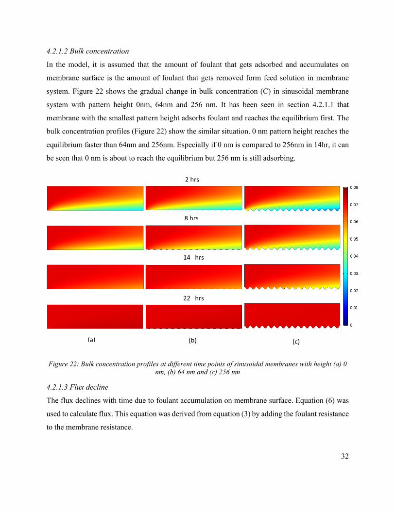
4.2.1.2 Bulk concentration

In the model, it is assumed that the amount of foulant that gets adsorbed and accumulates on

membrane surface is the amount of foulant that gets removed form feed solution in membrane

system. Figure 22 shows the gradual change in bulk concentration (C) in sinusoidal membrane

system with pattern height 0nm, 64nm and 256 nm. It has been seen in section 4.2.1.1 that

membrane with the smallest pattern height adsorbs foulant and reaches the equilibrium first. The

bulk concentration profiles (Figure 22) show the similar situation. 0 nm pattern height reaches the

equilibrium faster than 64nm and 256nm. Especially if 0 nm is compared to 256nm in 14hr, it can

be seen that 0 nm is about to reach the equilibrium but 256 nm is still adsorbing.

Figure 22: Bulk concentration profiles at different time points of sinusoidal membranes with height (a) 0 nm, (b) 64 nm and (c) 256 nm

4.2.1.3 Flux decline

The flux declines with time due to foulant accumulation on membrane surface. Equation (6) was

used to calculate flux. This equation was derived from equation (3) by adding the foulant resistance

to the membrane resistance.

2hrs

8hrs

14 hrs

22 hrsshrr

(a) (b) (c)

33

𝐹𝑙𝑢𝑥, 𝐽 = 𝑝 − ∆𝜋

𝜇𝑅< + 𝜇𝑅K (6)

𝑅K = 𝐶$𝐹 (7)

Here, Rf is foulant resistance and F is foulant coefficient.

F is the part of the equation that influence the effect of foulant accumulation on membrane surface

on flux decline. Several values for F were tried out to get the desired flux decline pattern that

agrees with Weinman and Husson’s experimental results (described in section 4.2.1.5) (Weinman

and Husson 2016). The value for F that was used here is 2.5×1013 m/mol.

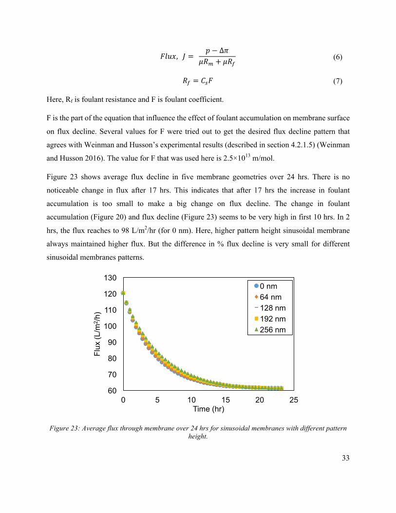
Figure 23 shows average flux decline in five membrane geometries over 24 hrs. There is no

noticeable change in flux after 17 hrs. This indicates that after 17 hrs the increase in foulant

accumulation is too small to make a big change on flux decline. The change in foulant

accumulation (Figure 20) and flux decline (Figure 23) seems to be very high in first 10 hrs. In 2

hrs, the flux reaches to 98 L/m2/hr (for 0 nm). Here, higher pattern height sinusoidal membrane

always maintained higher flux. But the difference in % flux decline is very small for different

sinusoidal membranes patterns.

Figure 23: Average flux through membrane over 24 hrs for sinusoidal membranes with different pattern height.

60

70

80

90

100

110

120

130

0 5 10 15 20 25

Flux

(L/m

2 /h)

Time (hr)

0 nm64 nm128 nm192 nm256 nm

34

Weinman and Husson (2016) presented their experimental findings as flux over time. They

presented the results for 120 mins for different membrane geometries. The simulation results of

this study for 120 mins and experimental results from Weinman and Husson are presented in

Figure 24. The flux decline trend in the model was similar to the experimental results. Although

the difference between flat and patterned membrane is not very big.

Figure 24: (a) Simulated and (b) experimental results for average flux through membrane over 120 mins (2hrs) for sinusoidal membrane geometries with different pattern height

(a)

(b)

35

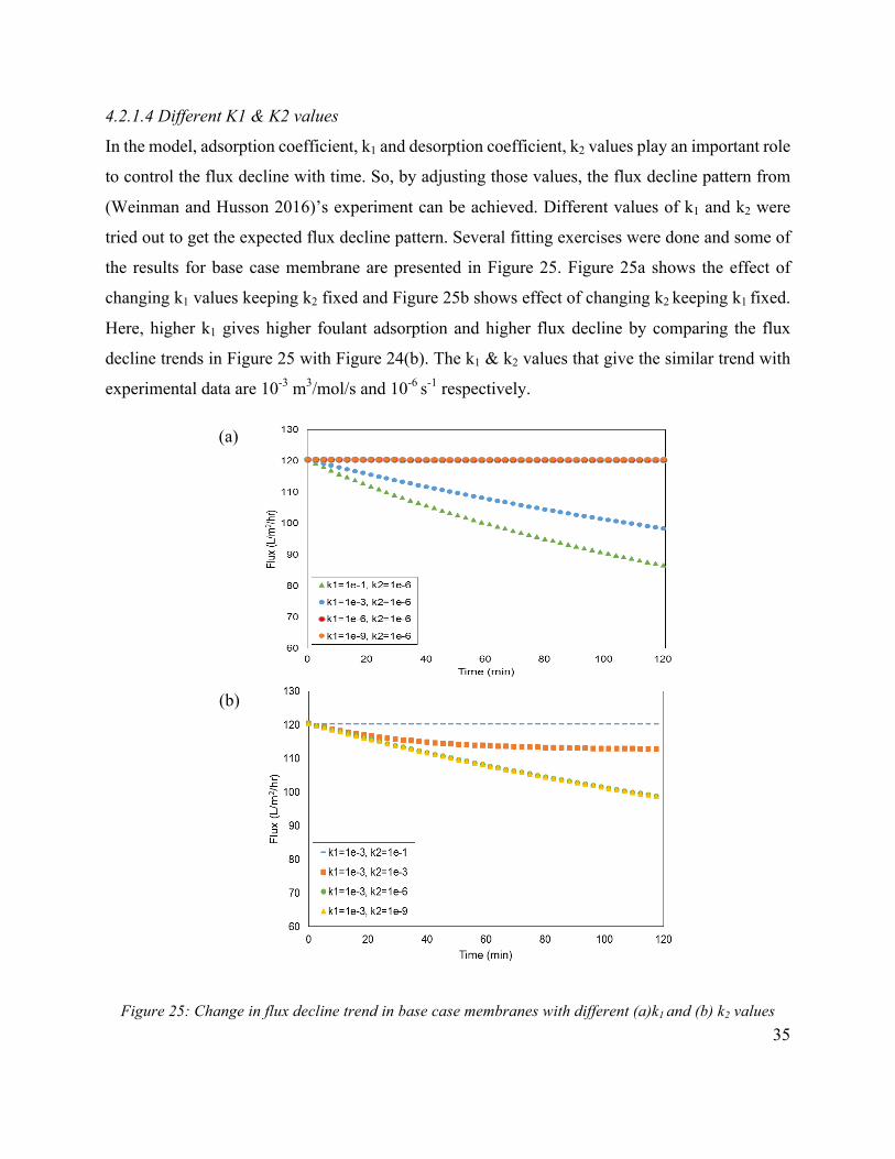
4.2.1.4 Different K1 & K2 values

In the model, adsorption coefficient, k1 and desorption coefficient, k2 values play an important role

to control the flux decline with time. So, by adjusting those values, the flux decline pattern from

(Weinman and Husson 2016)’s experiment can be achieved. Different values of k1 and k2 were

tried out to get the expected flux decline pattern. Several fitting exercises were done and some of

the results for base case membrane are presented in Figure 25. Figure 25a shows the effect of

changing k1 values keeping k2 fixed and Figure 25b shows effect of changing k2 keeping k1 fixed.

Here, higher k1 gives higher foulant adsorption and higher flux decline by comparing the flux

decline trends in Figure 25 with Figure 24(b). The k1 & k2 values that give the similar trend with

experimental data are 10-3 m3/mol/s and 10-6 s-1 respectively.

Figure 25: Change in flux decline trend in base case membranes with different (a)k1 and (b) k2 values

(a)

(b)

36

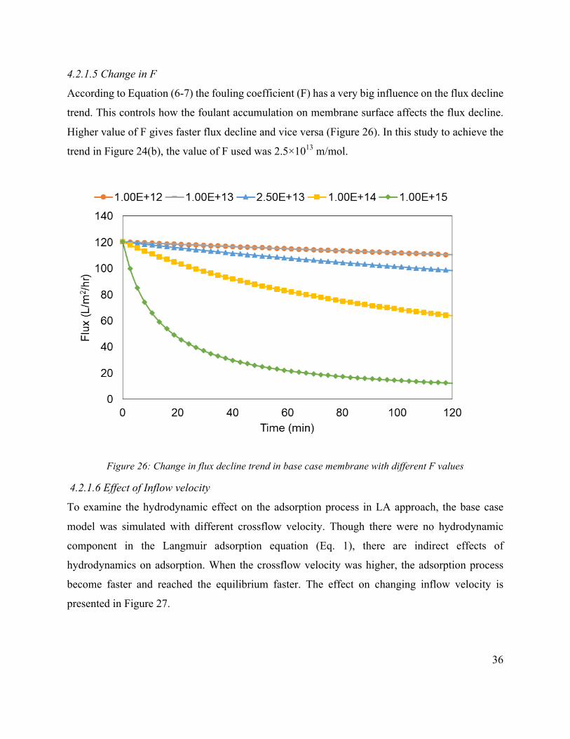
4.2.1.5 Change in F

According to Equation (6-7) the fouling coefficient (F) has a very big influence on the flux decline

trend. This controls how the foulant accumulation on membrane surface affects the flux decline.

Higher value of F gives faster flux decline and vice versa (Figure 26). In this study to achieve the

trend in Figure 24(b), the value of F used was 2.5×1013 m/mol.

Figure 26: Change in flux decline trend in base case membrane with different F values

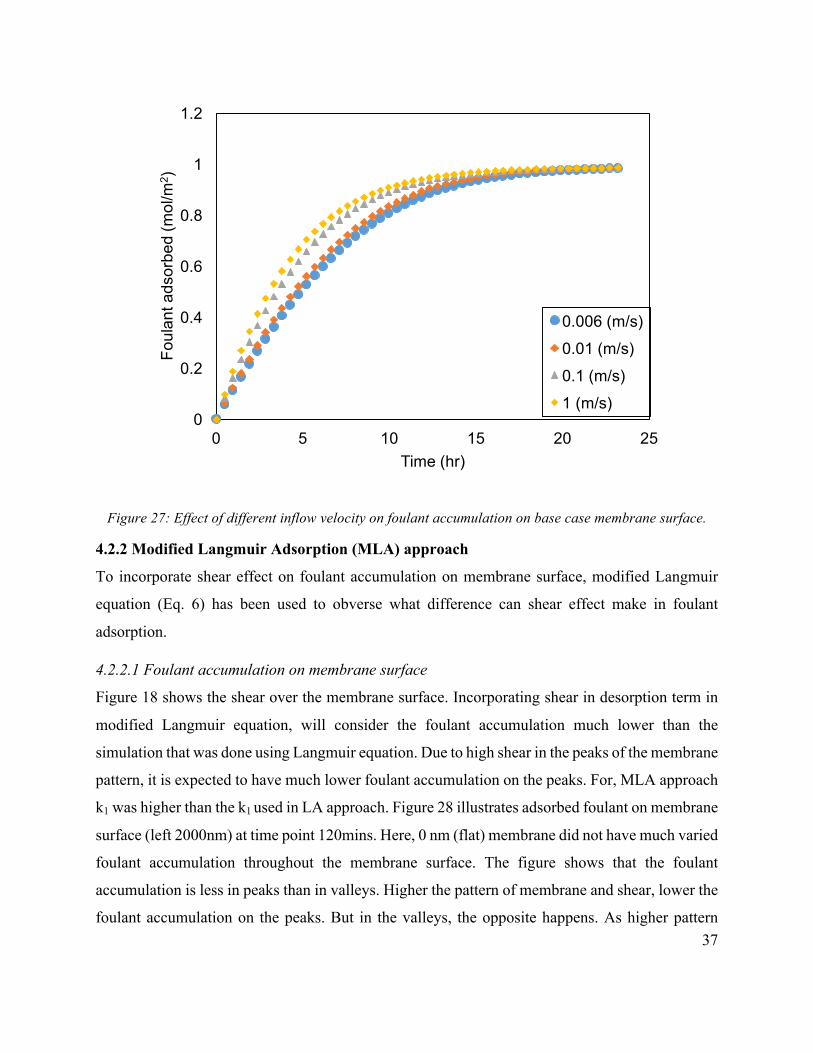
4.2.1.6 Effect of Inflow velocity

To examine the hydrodynamic effect on the adsorption process in LA approach, the base case

model was simulated with different crossflow velocity. Though there were no hydrodynamic

component in the Langmuir adsorption equation (Eq. 1), there are indirect effects of

hydrodynamics on adsorption. When the crossflow velocity was higher, the adsorption process

become faster and reached the equilibrium faster. The effect on changing inflow velocity is

presented in Figure 27.

37

Figure 27: Effect of different inflow velocity on foulant accumulation on base case membrane surface.

4.2.2 Modified Langmuir Adsorption (MLA) approach

To incorporate shear effect on foulant accumulation on membrane surface, modified Langmuir

equation (Eq. 6) has been used to obverse what difference can shear effect make in foulant

adsorption.

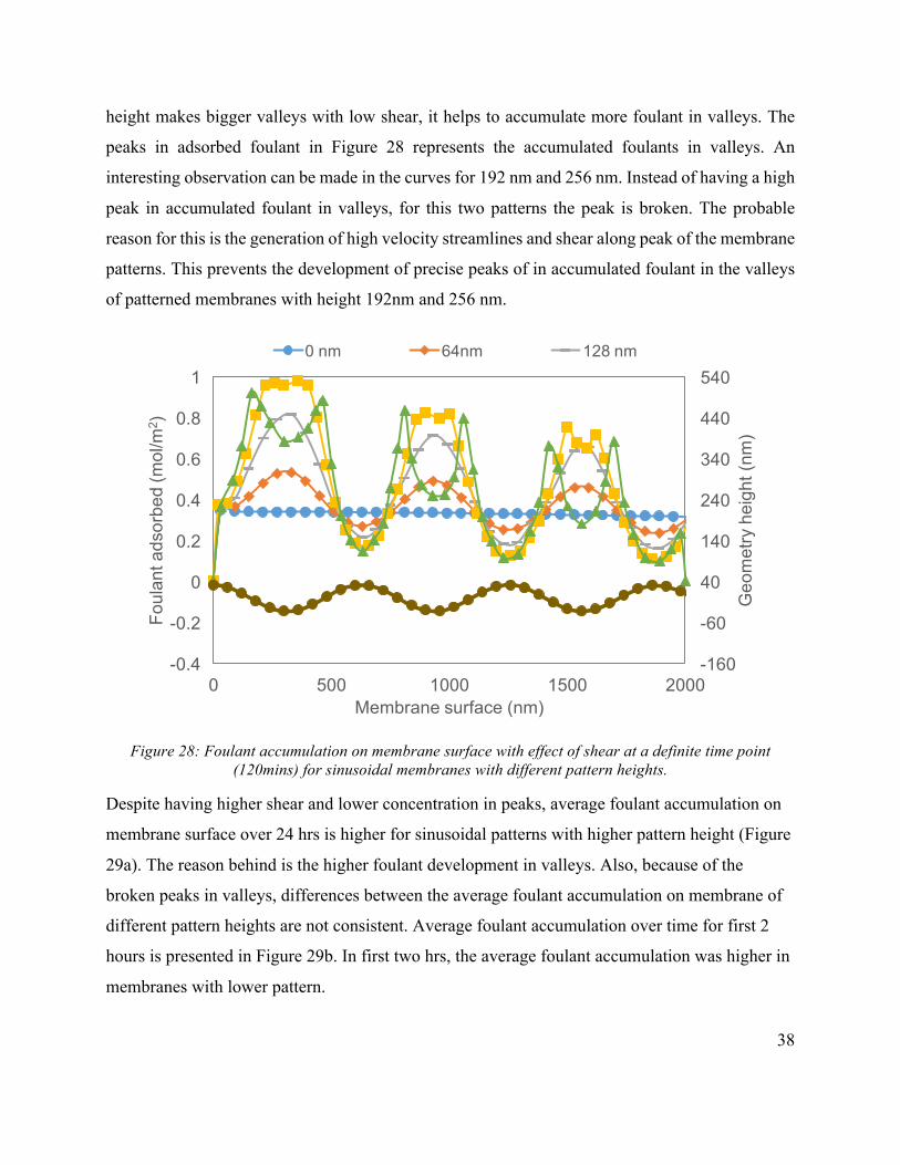
4.2.2.1 Foulant accumulation on membrane surface

Figure 18 shows the shear over the membrane surface. Incorporating shear in desorption term in

modified Langmuir equation, will consider the foulant accumulation much lower than the

simulation that was done using Langmuir equation. Due to high shear in the peaks of the membrane

pattern, it is expected to have much lower foulant accumulation on the peaks. For, MLA approach

k1 was higher than the k1 used in LA approach. Figure 28 illustrates adsorbed foulant on membrane

surface (left 2000nm) at time point 120mins. Here, 0 nm (flat) membrane did not have much varied

foulant accumulation throughout the membrane surface. The figure shows that the foulant

accumulation is less in peaks than in valleys. Higher the pattern of membrane and shear, lower the

foulant accumulation on the peaks. But in the valleys, the opposite happens. As higher pattern

0

0.2

0.4

0.6

0.8

1

1.2

0 5 10 15 20 25

Foul

ant a

dsor

bed

(mol

/m2 )

Time (hr)

0.006 (m/s)

0.01 (m/s)

0.1 (m/s)

1 (m/s)

38

height makes bigger valleys with low shear, it helps to accumulate more foulant in valleys. The

peaks in adsorbed foulant in Figure 28 represents the accumulated foulants in valleys. An

interesting observation can be made in the curves for 192 nm and 256 nm. Instead of having a high

peak in accumulated foulant in valleys, for this two patterns the peak is broken. The probable

reason for this is the generation of high velocity streamlines and shear along peak of the membrane

patterns. This prevents the development of precise peaks of in accumulated foulant in the valleys

of patterned membranes with height 192nm and 256 nm.

Figure 28: Foulant accumulation on membrane surface with effect of shear at a definite time point (120mins) for sinusoidal membranes with different pattern heights.

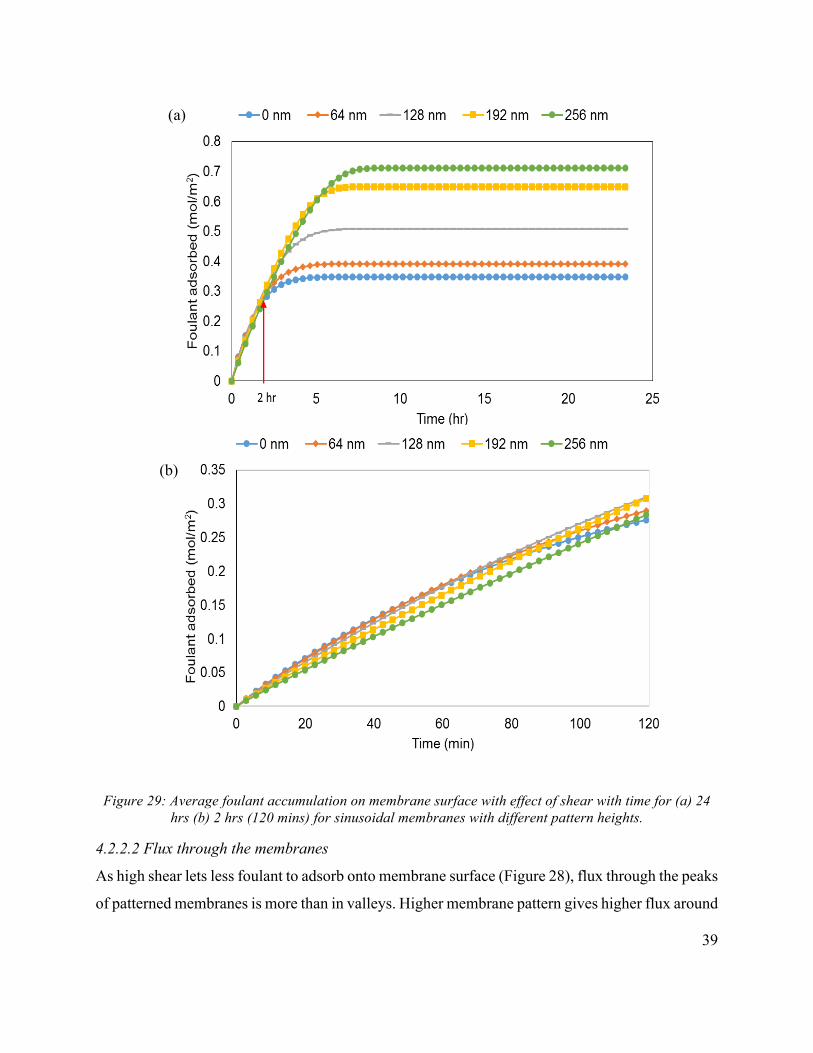
Despite having higher shear and lower concentration in peaks, average foulant accumulation on

membrane surface over 24 hrs is higher for sinusoidal patterns with higher pattern height (Figure

29a). The reason behind is the higher foulant development in valleys. Also, because of the

broken peaks in valleys, differences between the average foulant accumulation on membrane of

different pattern heights are not consistent. Average foulant accumulation over time for first 2

hours is presented in Figure 29b. In first two hrs, the average foulant accumulation was higher in

membranes with lower pattern.

-160

-60

40

140

240

340

440

540

-0.4

-0.2

0

0.2

0.4

0.6

0.8

1

0 500 1000 1500 2000

Geo

met

ry h

eigh

t (nm

)

Foul

ant a

dsor

bed

(mol

/m2 )

Membrane surface (nm)

0 nm 64nm 128 nm

39

Figure 29: Average foulant accumulation on membrane surface with effect of shear with time for (a) 24 hrs (b) 2 hrs (120 mins) for sinusoidal membranes with different pattern heights.

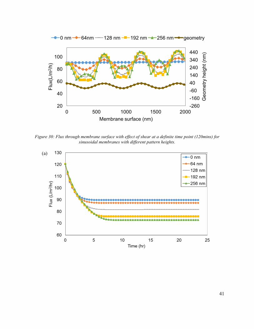
4.2.2.2 Flux through the membranes

As high shear lets less foulant to adsorb onto membrane surface (Figure 28), flux through the peaks

of patterned membranes is more than in valleys. Higher membrane pattern gives higher flux around

(b)

(a)

40

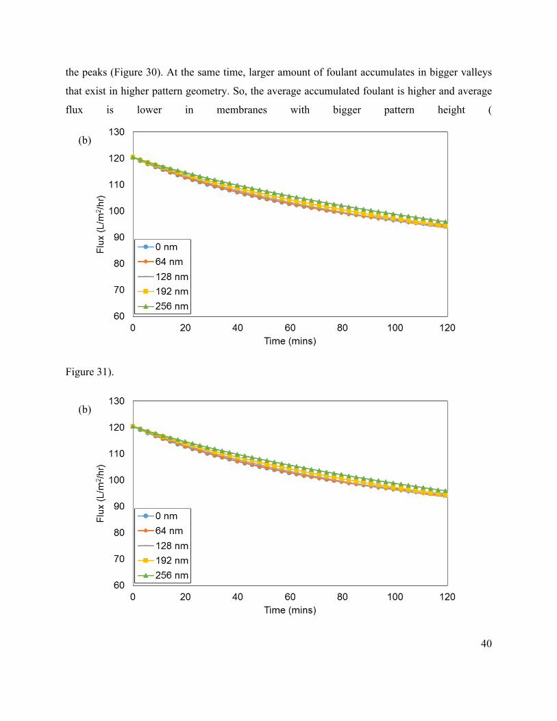
the peaks (Figure 30). At the same time, larger amount of foulant accumulates in bigger valleys

that exist in higher pattern geometry. So, the average accumulated foulant is higher and average

flux is lower in membranes with bigger pattern height (

Figure 31).

(b)

(b)

41

Figure 30: Flux through membrane surface with effect of shear at a definite time point (120mins) for sinusoidal membranes with different pattern heights.

-260-160-6040140240340440

20

40

60

80

100

0 500 1000 1500 2000

Geo

met

ry h

eigh

t (nm

)

Flux

(L/m

2 /h)

Membrane surface (nm)

0 nm 64nm 128 nm 192 nm 256 nm geometry

(a)

42

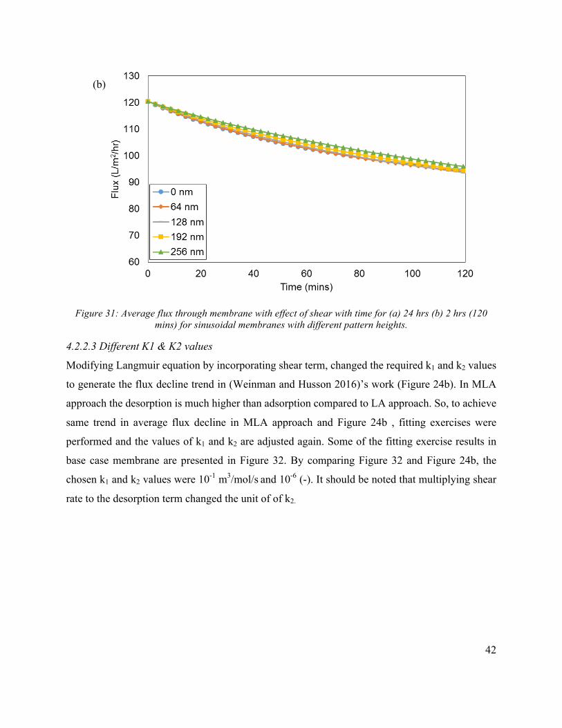
Figure 31: Average flux through membrane with effect of shear with time for (a) 24 hrs (b) 2 hrs (120 mins) for sinusoidal membranes with different pattern heights.

4.2.2.3 Different K1 & K2 values

Modifying Langmuir equation by incorporating shear term, changed the required k1 and k2 values

to generate the flux decline trend in (Weinman and Husson 2016)’s work (Figure 24b). In MLA

approach the desorption is much higher than adsorption compared to LA approach. So, to achieve

same trend in average flux decline in MLA approach and Figure 24b , fitting exercises were

performed and the values of k1 and k2 are adjusted again. Some of the fitting exercise results in

base case membrane are presented in Figure 32. By comparing Figure 32 and Figure 24b, the

chosen k1 and k2 values were 10-1 m3/mol/s and 10-6 (-). It should be noted that multiplying shear

rate to the desorption term changed the unit of of k2.

(b)

43

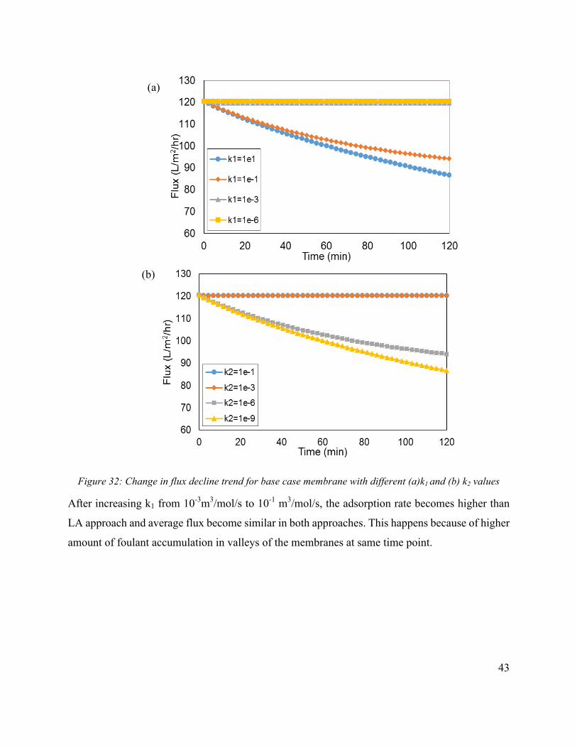
Figure 32: Change in flux decline trend for base case membrane with different (a)k1 and (b) k2 values

After increasing k1 from 10-3m3/mol/s to 10-1 m3/mol/s, the adsorption rate becomes higher than

LA approach and average flux become similar in both approaches. This happens because of higher

amount of foulant accumulation in valleys of the membranes at same time point.

(a)

(b)

44

Figure 33: Accumulated foulnt on membrane surface after 120 mins for (a) k 1= 10-1 m3/mol/s, k2 = 10-6 (b) k1 = 10-3m3/mol/s, k2 = 10-6

-100

0

100

200

300

400

500

600

-0.4

-0.2

0

0.2

0.4

0.6

0.8

1

0 500 1000 1500 2000

Geo

met

ry h

eigh

t (nm

)

Foul

ant a

dsor

bed

(mol

/m2)

Membrane surface (nm)

0 nm 64nm 128 nm 192 nm 256 nm geometry(a)

-100

0

100

200

300

400

500

600

-0.4

-0.2

0

0.2

0.4

0.6

0.8

1

0 500 1000 1500 2000

Geo

met

ry h

eigh

t (nm

)

Foul

ant a

dsor

bed

(mol

/m2)

Membrane surface (nm)

0 nm 64nm 128 nm 192 nm 256 nm geometry(b)

45

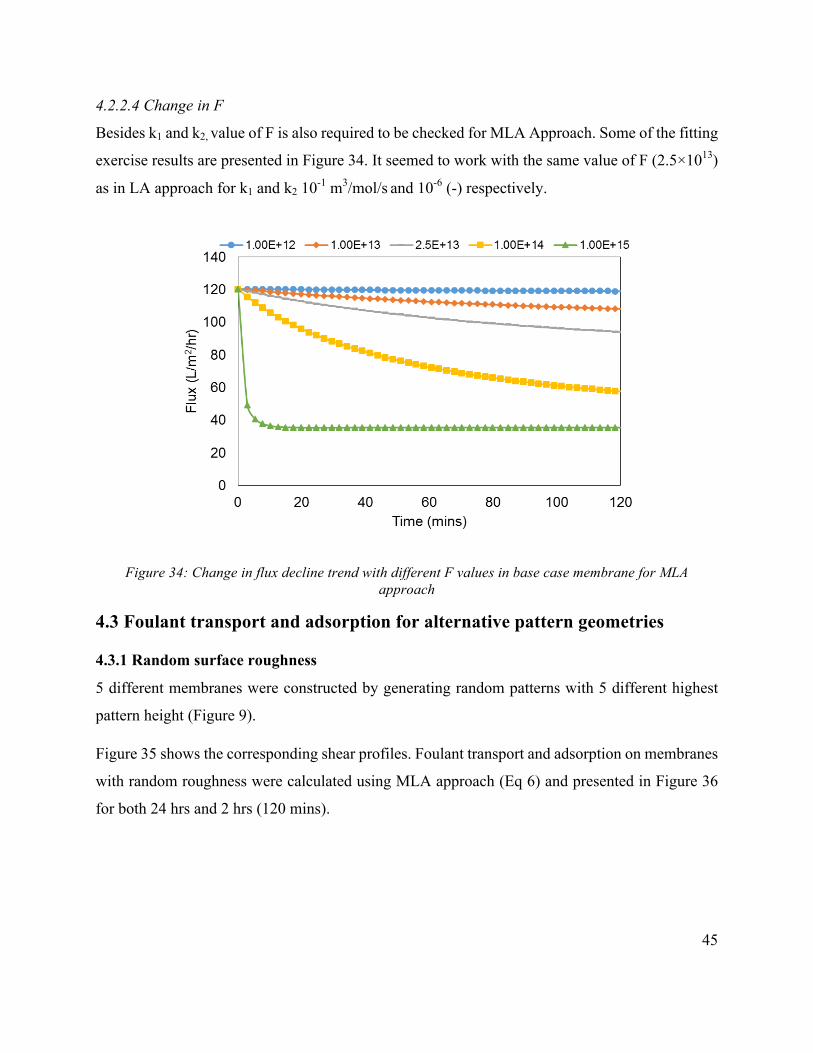
4.2.2.4 Change in F

Besides k1 and k2, value of F is also required to be checked for MLA Approach. Some of the fitting

exercise results are presented in Figure 34. It seemed to work with the same value of F (2.5×1013)

as in LA approach for k1 and k2 10-1 m3/mol/s and 10-6 (-) respectively.

Figure 34: Change in flux decline trend with different F values in base case membrane for MLA approach

4.3 Foulant transport and adsorption for alternative pattern geometries

4.3.1 Random surface roughness

5 different membranes were constructed by generating random patterns with 5 different highest

pattern height (Figure 9).

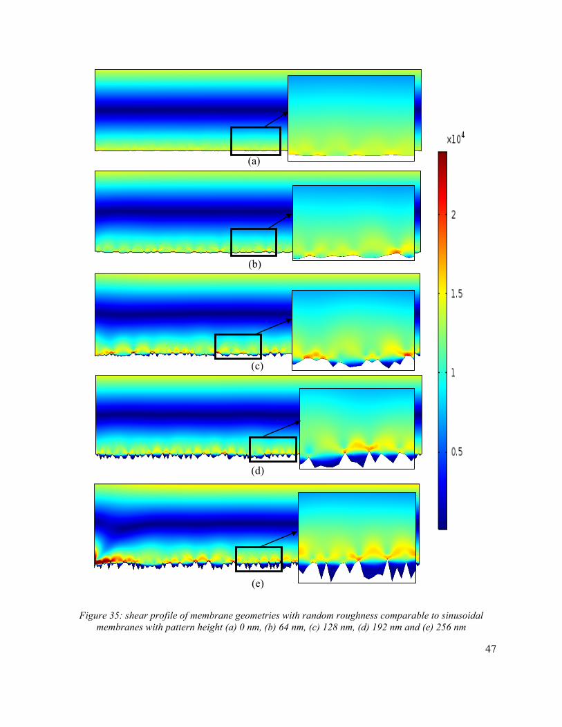
Figure 35 shows the corresponding shear profiles. Foulant transport and adsorption on membranes

with random roughness were calculated using MLA approach (Eq 6) and presented in Figure 36

for both 24 hrs and 2 hrs (120 mins).

46

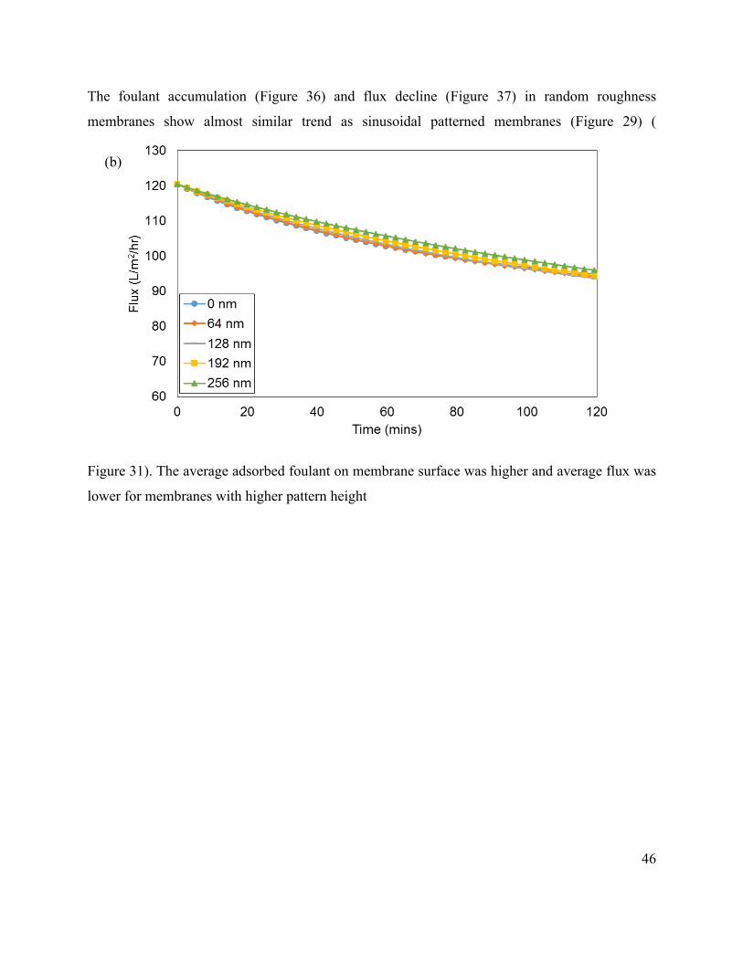
The foulant accumulation (Figure 36) and flux decline (Figure 37) in random roughness

membranes show almost similar trend as sinusoidal patterned membranes (Figure 29) (

Figure 31). The average adsorbed foulant on membrane surface was higher and average flux was

lower for membranes with higher pattern height

(b)

47

Figure 35: shear profile of membrane geometries with random roughness comparable to sinusoidal membranes with pattern height (a) 0 nm, (b) 64 nm, (c) 128 nm, (d) 192 nm and (e) 256 nm

(a)

(b)

(c)

(d)

(e)

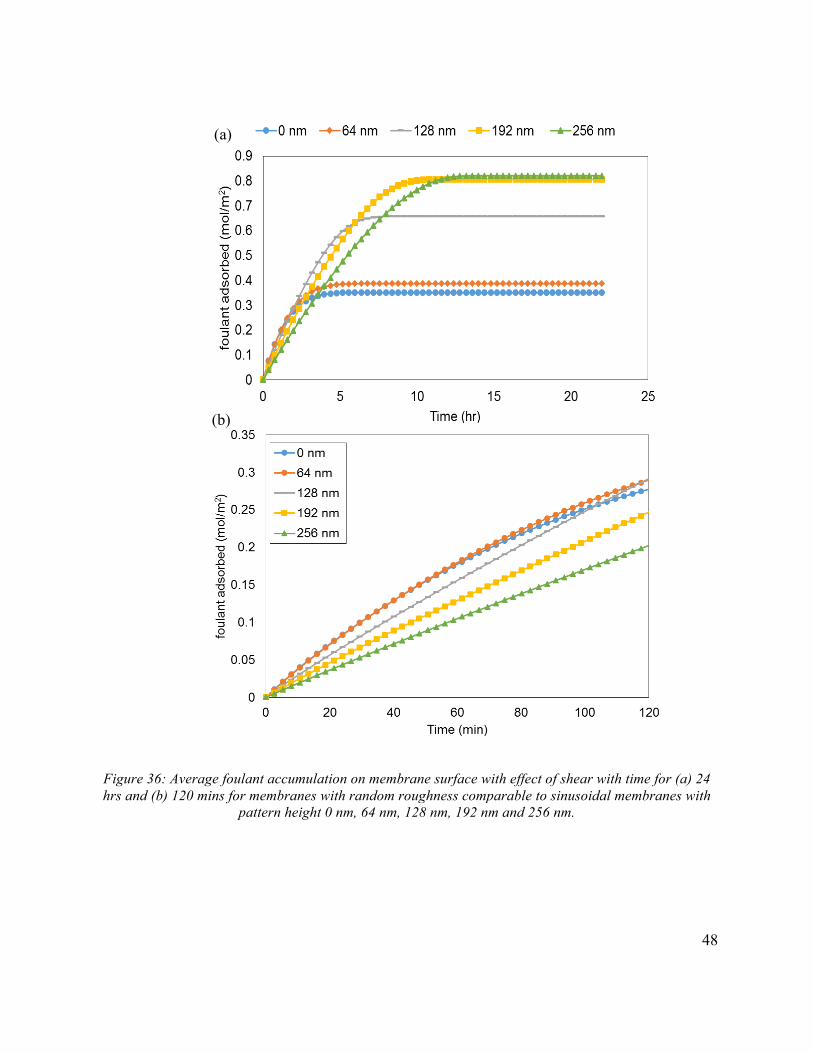
48

Figure 36: Average foulant accumulation on membrane surface with effect of shear with time for (a) 24 hrs and (b) 120 mins for membranes with random roughness comparable to sinusoidal membranes with

pattern height 0 nm, 64 nm, 128 nm, 192 nm and 256 nm.

(a)

(b)

49

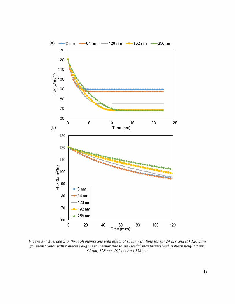
Figure 37: Average flux through membrane with effect of shear with time for (a) 24 hrs and (b) 120 mins for membranes with random roughness comparable to sinusoidal membranes with pattern height 0 nm,

64 nm, 128 nm, 192 nm and 256 nm.

(a)

(b)

50

To make direct comparison, percentage of flux decline in 24hrs for both random roughness

membrane and sinusoidal membranes are plotted in Figure 38. For both kind of membranes, flux

decline increased for higher pattern height. Also, sinusoidal membranes mostly maintained lower

flux decline than random roughness membrane. Higher the pattern height gets, more visible the

differences in flux decline between two kinds of membranes become. This indicates more foulants

accumulate in membranes with random roughness than in membranes with sinusoidal patterns

with.

Figure 38: Comparison of percentage of flux decline after 24 hrs for membranes with random roughness to sinusoidal patterned membranes.

4.3.2 Other geometrical patterns

As seen in Figure 28, less fouling can only be achieved near the peaks of sinusoidal membrane

patterns. But because of the existence of deep valleys, more foulant accumulates there compared

to the amount of foulant that gets removed due to shear. So, if a geometry that has shallower valleys

can give better results.

51

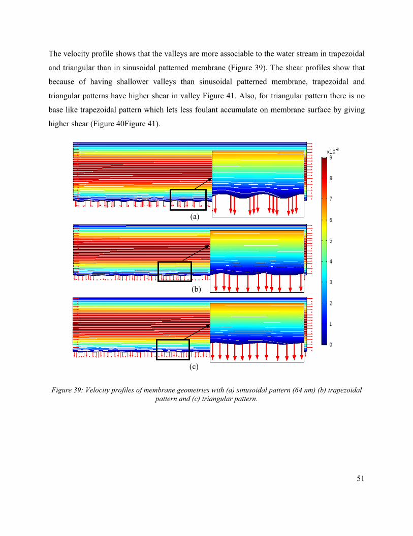
The velocity profile shows that the valleys are more associable to the water stream in trapezoidal

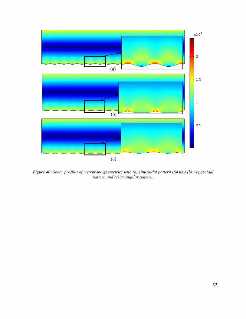
and triangular than in sinusoidal patterned membrane (Figure 39). The shear profiles show that

because of having shallower valleys than sinusoidal patterned membrane, trapezoidal and

triangular patterns have higher shear in valley Figure 41. Also, for triangular pattern there is no

base like trapezoidal pattern which lets less foulant accumulate on membrane surface by giving

higher shear (Figure 40Figure 41).

Figure 39: Velocity profiles of membrane geometries with (a) sinusoidal pattern (64 nm) (b) trapezoidal pattern and (c) triangular pattern.

(a)

(b)

(c)

52

Figure 40: Shear profiles of membrane geometries with (a) sinusoidal pattern (64 nm) (b) trapezoidal pattern and (c) triangular pattern.

(a)

(b)

(c)

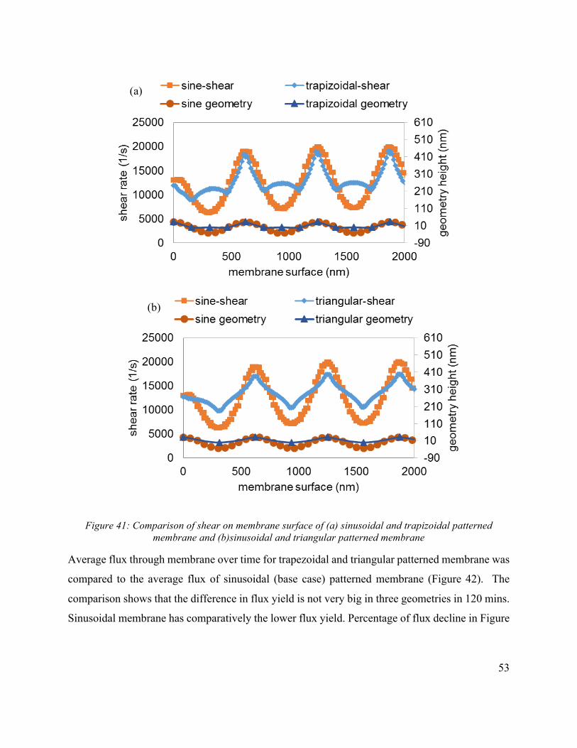
53

Figure 41: Comparison of shear on membrane surface of (a) sinusoidal and trapizoidal patterned membrane and (b)sinusoidal and triangular patterned membrane

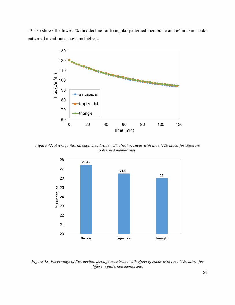
Average flux through membrane over time for trapezoidal and triangular patterned membrane was

compared to the average flux of sinusoidal (base case) patterned membrane (Figure 42). The

comparison shows that the difference in flux yield is not very big in three geometries in 120 mins.

Sinusoidal membrane has comparatively the lower flux yield. Percentage of flux decline in Figure

(b)

(a)

54

43 also shows the lowest % flux decline for triangular patterned membrane and 64 nm sinusoidal

patterned membrane show the highest.

Figure 42: Average flux through membrane with effect of shear with time (120 mins) for different patterned membranes.

Figure 43: Percentage of flux decline through membrane with effect of shear with time (120 mins) for different patterned membranes

55

5 Other efforts Some other efforts were approached during this study but were not pursued further due to

convergence limitation.

5.1 Additional Shear Term

In the MLA approach (Eq 6) that has been discussed in section 4.2.2, the shear rate was multiplied

to the desorption term of Langmuir equation to incorporate direct shear effect on adsorption.

Another effort for modification of Langmuir adsorption equation was equation 10.

𝑑𝐶$𝑑𝑡 = 𝐾&𝐶 𝐶$( − 𝐶$ −𝐾"𝐶$ − 𝑅$ (8)

𝑅$ = 𝑘M𝑐$𝜏 (9)

Here, Rs is the shear term and k3 is shear coefficient. This shear tern adds to desorption term to

include the effect of shear to desorption.

But this effort for modification was unsuccessful because the simulation became complicated and

almost impossible to converge the model to have successful results. The model only converged

and was able to give solution for only very small values of k3 which made Rs term so small that it

had hardly any effect on adsorption. The effect of shear was hardly seen.

5.2 One Step Study

To construct simpler model and make simulations easier, the hydrodynamics and foulant

adsorption equations were combined and incorporated to a one step steady state model. Like it is

explained in section 3.2.1, instead of using the equation (3), equation (6) was used which directly

calculates flux after considering adsorbed foulant (cs) on membrane surface. The model calculated

cs using the equation (12) which was derived from Modified Langmuir adsorption equation (Eq.

5) considering steady state.

𝑐$ =1000 ∗ 𝑘& ∗ 𝑐𝑘& ∗ 𝑐 + 𝑘" ∗ 𝜏

(10)

56

But the major problem with this effort also was convergence. The components of the equations

were inter-dependent. It became very difficult to get the desired trend in hydrodynamics and flux

output as the model converged for limited number of values of K1, K2 and F.

6 Future work

6.1 Particle tracing

The model was completely an adsorption model in this study. So foulant accumulation on

membrane surface solely dependent on the defined adsorption equation and foulant was considered

here as concentration. To evaluate the foulant particle interaction with membrane surface, the next

step should be particle tracing approach. Here, foulants are considered as particles with definite

diameter and number of foulant particles that enters the system can be defined. Depending on the

hydrodynamic conditions the particles will flow through the system. While flowing through it can

interact to the obstructions that it encounters on its way and depending on hydrodynamics it can

get stuck or flow by. This approach will help to understand precisely how can foulants get

removed, how much area gets covered by foulant and what are the effects of changing membrane

structures.

6.2 Turbulent Modelling

In this study the flow was considered as Laminar flow. Although the parameters for the model

were taken from Weinman and Husson’s work (Weinman and Husson 2016) and the crossflow

velocity they used was 1 m/s. It was downscaled for this study. But the next modelling step can be

defining the flow behavior as turbulent flow.

6.3 Effect of concentration polarization

Effect of concentration polarization is not simulated in this study. So, to include that, change of

boundary conditions like flux yield through membrane and adding salt concentration can be

considered. Also, as described in 6.1, Particle tracing also a good way to simulate membrane

filtration system with concentration polarization.

57

6.4 3D modeling

For this study, the simulated geometries were 2D. Converting these models to 3D can be a good

way to have simulation results which agree more to the practical data.

6 Conclusion CFD Simulations illustrated two approaches with indirect (LA) and direct (MLA) effect of

hydrodynamics during adsorption. Simulation showed that with LA approach higher sinusoidal

patterns accumulate less amount of foulant and flux decline on membrane surface. But the

differences between sinusoidal pattern height needs to be significant to have a noticeable change.

LA approach was able to show the similar trend in flux decline for both membranes with 0 nm and

64nm (base case) pattern height in simulated and experimental data of Weinman and Husson

(Weinman and Husson 2016) (Figure 24b).. The difference between average fluxes for these two

membranes were very small in both cases. But in LA approach the foulant accumulation was high

is peaks and low in valleys. This shows that this approach does not consider any shear stress that

is caused by water stream in the system. Also, sinusoidal membranes with higher patterns were

showing less fouling because of bigger surface area than a membrane with smaller sinusoidal

pattern height.

MLA approach had direct effect of hydrodynamics and it showed shear can play a big role in

fouling mitigation in patterned membranes. Higher sinusoidal patterned membranes had higher

shear along their peaks which kept the flux high in that area. But it was also seen that, because of

more foulant accumulation in valleys of membranes with higher sinusoidal pattern height, the

average calculated foulant accumulation and flux decline was higher with time compared to the

membranes with smaller pattern height.

Membranes with random roughness were seen to have higher foulant accumulation and flux

decline with time compared to sinusoidal patterned membranes when simulated using MLA

approach. But, trapezoidal and triangular patterns with same period and half of the pattern height

of sinusoidal base case membrane were seen to accumulate less foulant and have less flux decline.

58

8 References Al-Amoudi, Ahmed, and Robert W. Lovitt. 2007. “Fouling Strategies and the Cleaning System of

NF Membranes and Factors Affecting Cleaning Efficiency.” Journal of Membrane Science

303 (1): 4–28. doi:10.1016/j.memsci.2007.06.002.

Al-Amoudi, Ahmed Saleh. 2010. “Factors Affecting Natural Organic Matter (NOM) and Scaling

Fouling in NF Membranes: A Review.” Desalination 259 (1): 1–10.

doi:10.1016/j.desal.2010.04.003.

Bellona, Christopher, Jog E Drewes, Pei Xu, and Gary Amy. 2004. “Factors Affecting the

Rejection of Organic Solutes during NF/RO Treatment—a Literature Review ARTICLE IN

PRESS.” Water Research 38: 2795–2809. doi:10.1016/j.watres.2004.03.034.

Bikel, Matías, Ineke G. M. Pünt, Rob G. H. Lammertink, and Matthias Wessling. 2009.

“Micropatterned Polymer Films by Vapor-Induced Phase Separation Using Permeable

Molds.” ACS Applied Materials & Interfaces 1 (12). American Chemical Society: 2856–61.

doi:10.1021/am900594p.

Bowen, W.Richard, Teodora A. Doneva, and H.B. Yin. 2002. “Atomic Force Microscopy Studies

of Membrane—solute Interactions (Fouling).” Desalination 146 (1–3): 97–102.

doi:10.1016/S0011-9164(02)00496-4.

Cheryan, Munir., and Munir. Cheryan. 1998. Ultrafiltration and Microfiltration Handbook.

Technomic Pub. Co.

Chou, Stephen Y. 1996. “Nanoimprint Lithography.” Journal of Vacuum Science & Technology

B: Microelectronics and Nanometer Structures 14 (6): 4129. doi:10.1116/1.588605.

Clark, Mark M. 2009. Transport Modeling for Environmental Engineers and Scientists. Wiley.

http://www.wiley.com/WileyCDA/WileyTitle/productCd-0470260726,subjectCd-

CH22.html.

Comsol. 2016. “Detailed Explanation of the Finite Element Method (FEM).” Comsol Website.

https://www.comsol.com/multiphysics/finite-element-method.

59

Çulfaz, P. Zeynep, Steffen Buetehorn, Lavinia Utiu, Markus Kueppers, Bernhard Bluemich,

Thomas Melin, Matthias Wessling, and Rob G. H. Lammertink. 2011. “Fouling Behavior of

Microstructured Hollow Fiber Membranes in Dead-End Filtrations: Critical Flux

Determination and NMR Imaging of Particle Deposition.” Langmuir 27 (5). American

Chemical Society: 1643–52. doi:10.1021/la1037734.

Demneh, Seyedeh Marzieh Ghasemi, Bahram Nasernejad, and Hamid Modarres. 2011. “Modeling

Investigation of Membrane Biofouling Phenomena by Considering the Adsorption of Protein,

Polysaccharide and Humic Acid.” Colloids and Surfaces B: Biointerfaces 88 (1): 108–14.

doi:10.1016/j.colsurfb.2011.06.018.

Ding, Yifu, Sajjad Maruf, Masoud Aghajani, and Alan R. Greenberg. 2016a. “Surface Patterning

of Polymeric Membranes and Its Effect on Antifouling Characteristics.” Separation Science

and Technology 6395 (July): 1–18. doi:10.1080/01496395.2016.1201115.

———. 2016b. “Surface Patterning of Polymeric Membranes and Its Effect on Antifouling

Characteristics.” Separation Science and Technology 6395 (July): 01496395.2016.1201115.

doi:10.1080/01496395.2016.1201115.

Ding, Yifu, Jirun Sun, Hyun Wook Ro, Zhen Wang, Jing Zhou, Nancy J. Lin, Marcus T. Cicerone,

Christopher L. Soles, and Sheng Lin-Gibson. 2011. “Thermodynamic Underpinnings of Cell

Alignment on Controlled Topographies.” Advanced Materials 23 (3). WILEY-VCH Verlag:

421–25. doi:10.1002/adma.201001757.

Drewes, J, and P Fox. 1999. “Fate of Natural Organic Matter (NOM) during Ground Water

Recharge Using Reclaimed Water.” Water Science and Technology 40 (9). IWA Publishing:

241–48. doi:10.1016/S0273-1223(99)00662-9.

Feng, X. J., and L. Jiang. 2006. “Design and Creation of Superwetting/Antiwetting Surfaces.”

Advanced Materials 18 (23). WILEY-VCH Verlag: 3063–78. doi:10.1002/adma.200501961.

Frei, Walter. 2013. “Meshing Considerations for Linear Static Problems | COMSOL Blog.”

Comsol Blog. https://www.comsol.com/blogs/meshing-considerations-linear-static-

problems/.

60

Gença, Y., E. N. Durmaz, and P. Z. Çulfaz-Emecen. 2015. “Preparation of Patterned

Microfiltration Membranes and Their Performance in Crossflow Yeast Filtration.” Journal of

Membrane Science 476: 224–33. doi:10.1016/j.memsci.2014.11.041.

Gironès, M., I.J. Akbarsyah, W. Nijdam, C.J.M. van Rijn, H.V. Jansen, R.G.H. Lammertink, and

M. Wessling. 2006. “Polymeric Microsieves Produced by Phase Separation Micromolding.”

Journal of Membrane Science 283 (1): 411–24. doi:10.1016/j.memsci.2006.07.016.

Guo, L. J. 2007. “Nanoimprint Lithography: Methods and Material Requirements.” Advanced

Materials 19 (4). WILEY-VCH Verlag: 495–513. doi:10.1002/adma.200600882.

Ho, W. S. Winston, and Kamalesh K. Sirkar. 1992. “Overview.” In Membrane Handbook, 3–15.

Boston, MA: Springer US. doi:10.1007/978-1-4615-3548-5_1.

Jang, Jun Hee, Jaewoo Lee, Seon Yeop Jung, Dong Chan Choi, Young June Won, Kyung Hyun

Ahn, Pyung Kyu Park, and Chung Hak Lee. 2015. “Correlation between Particle Deposition

and the Size Ratio of Particles to Patterns in Nano- and Micro-Patterned Membrane Filtration

Systems.” Separation and Purification Technology 156. Elsevier B.V.: 608–16.

doi:10.1016/j.seppur.2015.10.056.

Jarusutthirak, Chalor, Gary Amy, and Jean-Philippe Croué. 2002. “Fouling Characteristics of

Wastewater Effluent Organic Matter (EfOM) Isolates on NF and UF Membranes.”

Desalination 145 (1–3): 247–55. doi:10.1016/S0011-9164(02)00419-8.

Jones, Kimberly L., and Charles R. O’Melia. 2000. “Protein and Humic Acid Adsorption onto

Hydrophilic Membrane Surfaces: Effects of pH and Ionic Strength.” Journal of Membrane

Science 165 (1): 31–46. doi:10.1016/S0376-7388(99)00218-5.

Kang, Guo-dong, and Yi-ming Cao. 2012. “Development of Antifouling Reverse Osmosis

Membranes for Water Treatment: A Review.” Water Research 46 (3): 584–600.

doi:10.1016/j.watres.2011.11.041.

Kao, C. M., B. M. Yang, R. Y. Surampalli, and Tian C. Zhang. 2012. “Limitation of Membrane

Technology and Prevention of Membrane Fouling.” In Membrane Technology and

Environmental Applications, 504–32. Reston, VA: American Society of Civil Engineers.

61

doi:10.1061/9780784412275.ch17.

Lee, Young Ki, Young June Won, Jae Hyun Yoo, Kyung Hyun Ahn, and Chung Hak Lee. 2013.

“Flow Analysis and Fouling on the Patterned Membrane Surface.” Journal of Membrane

Science 427. Elsevier: 320–25. doi:10.1016/j.memsci.2012.10.010.

Lim, A. L., and Renbi Bai. 2003. “Membrane Fouling and Cleaning in Microfiltration of Activated

Sludge Wastewater.” Journal of Membrane Science 216 (1–2): 279–90. doi:10.1016/S0376-

7388(03)00083-8.

Maruf, Sajjad H., Melissa Rickman, Liang Wang, John Mersch IV, Alan R. Greenberg, John

Pellegrino, and Yifu Ding. 2013. “Influence of Sub-Micron Surface Patterns on the

Deposition of Model Proteins during Active Filtration.” Journal of Membrane Science 444.

Elsevier: 420–28. doi:10.1016/j.memsci.2013.05.060.

Maruf, Sajjad H., Liang Wang, Alan R. Greenberg, John Pellegrino, and Yifu Ding. 2013. “Use

of Nanoimprinted Surface Patterns to Mitigate Colloidal Deposition on Ultrafiltration

Membranes.” Journal of Membrane Science 428. Elsevier: 598–607.

doi:10.1016/j.memsci.2012.10.059.

Petronis, Šarūnas, Kent Berntsson, Julie Gold, and Paul Gatenholm. 2000. “Design and

Microstructuring of PDMS Surfaces for Improved Marine Biofouling Resistance.” Journal

of Biomaterials Science, Polymer Edition 11 (10). Taylor & Francis Group : 1051–72.

doi:10.1163/156856200743571.

Ro, Hyun Wook, Vera Popova, Lei Chen, Aaron M. Forster, Yifu Ding, Kyle J. Alvine, Dave J.

Krug, Richard M. Laine, and Christopher L. Soles. 2011. “Cubic Silsesquioxanes as a Green,

High-Performance Mold Material for Nanoimprint Lithography.” Advanced Materials 23 (3).

WILEY-VCH Verlag: 414–20. doi:10.1002/adma.201001761.

Sagle, Alyson C., Elizabeth M. Van Wagner, Hao Ju, Bryan D. McCloskey, Benny D. Freeman,

and Mukul M. Sharma. 2009. “PEG-Coated Reverse Osmosis Membranes: Desalination

Properties and Fouling Resistance.” Journal of Membrane Science 340 (1–2): 92–108.

doi:10.1016/j.memsci.2009.05.013.

62

Sayed, S K I. 2010. “OPTIMUM OPERATION CONDITIONS OF DIRECT CAPILLARY

NANOFILTRATION FOR WASTEWATER TREATMENT” 14.

http://www.iwtc.info/2010_pdf/08-04.pdf.

Šereš, Zita, Dragana Šoronja Simović, Ljubica Dokić, Lidietta Giorno, Biljana Pajin, Cecilia

Hodur, and Nikola Maravić. 2016. “Edible Oil Industry Wastewater Treatment by

Microfiltration with Ceramic Membrane.” World Academy of Science, Engineering and

Technology, International Journal of Chemical, Molecular, Nuclear, Materials and

Metallurgical Engineering 10 (4): 410–13. https://waset.org/Publication/edible-oil-industry-

wastewater-treatment-by-microfiltration-with-ceramic-membrane/10004151.

Singh, Rajindar. 2006. Hybrid Membrane Systems for Water Purification : Technology, Systems

Design and Operation. Elsevier.

Stroock, Abraham D., Stephan K. W. Dertinger, Armand Ajdari, Igor Mezić, Howard A. Stone,

and George M. Whitesides. 2002. “Chaotic Mixer for Microchannels.” Science 295 (5555).

http://science.sciencemag.org/content/295/5555/647.

Verliefde, Arne, Emile Cornelissen, Gary Amy, Bart Van Der Bruggen, and Hans Van Dijk. 2017.

“Priority Organic Micropollutants in Water Sources in Flanders and the Netherlands and

Assessment of Removal Possibilities with Nanofiltration.” Accessed April 21.

doi:10.1016/j.envpol.2006.01.051.

Vogelaar, L., J.N. Barsema, C.J.M. van Rijn, W. Nijdam, and M. Wessling. 2003. “Phase

Separation Micromolding—PSµM.” Advanced Materials 15 (16). WILEY-VCH Verlag:

1385–89. doi:10.1002/adma.200304949.

Vogelaar, Laura, Rob G. H. Lammertink, Jonathan N. Barsema, Wietze Nijdam, Lydia A. M.

Bolhuis-Versteeg, Cees J. M. van Rijn, and Matthias Wessling. 2005. “Phase Separation

Micromolding: A New Generic Approach for Microstructuring Various Materials.” Small 1

(6). WILEY-VCH Verlag: 645–55. doi:10.1002/smll.200400128.

Vrijenhoek, Eric M, Seungkwan Hong, and Menachem Elimelech. 2001. “Influence of Membrane

Surface Properties on Initial Rate of Colloidal Fouling of Reverse Osmosis and Nanofiltration

63

Membranes.” Journal of Membrane Science 188: 115–28.

http://citeseerx.ist.psu.edu/viewdoc/download?doi=10.1.1.515.5946&rep=rep1&type=pdf.

Vrouwenvelder, J.S., J.A.M. van Paassen, L.P. Wessels, A.F. van Dam, and S.M. Bakker. 2006.

“The Membrane Fouling Simulator: A Practical Tool for Fouling Prediction and Control.”

Journal of Membrane Science 281 (1): 316–24. doi:10.1016/j.memsci.2006.03.046.

Wang, Zhen, and Yifu Ding. 2010. “Probing Polymer Deformation Profiles at Varying Depths in

Nanoimprint Lithography.” Nanotechnology 21 (10). IOP Publishing: 105301.

doi:10.1088/0957-4484/21/10/105301.

Weinman, Steven T., and Scott M. Husson. 2016. “Influence of Chemical Coating Combined with

Nanopatterning on Alginate Fouling during Nanofiltration.” Journal of Membrane Science

513: 146–54. doi:10.1016/j.memsci.2016.04.025.

Won, Young June, Seon Yeop Jung, June Hee Jang, Jae Woo Lee, Hee Ro Chae, Dong Chan Choi,

Kyung Hyun Ahn, Chung Hak Lee, and Pyung Kyu Park. 2016. “Correlation of Membrane

Fouling with Topography of Patterned Membranes for Water Treatment.” Journal of

Membrane Science 498: 14–19. doi:10.1016/j.memsci.2015.09.058.

Won, Young June, Jaewoo Lee, Dong Chan Choi, Hee Ro Chae, Inae Kim, Chung Hak Lee, and

In Chul Kim. 2012. “Preparation and Application of Patterned Membranes for Wastewater

Treatment.” Environmental Science and Technology 46 (20): 11021–27.

doi:10.1021/es3020309.

Xie, Peng, Lawrence Murdoch, and David Ladner. 2016. “Comparison of Computational Fluid

Dynamics (CFD) and Experimental Data for Fouling Mitigation with Sinusoidal Reverse

Osmosis Spacer.” ( In Process). Accessed November 2.

http://www.awwa.org/portals/0/files/education/conferences/membrane/mtc16/membrane

papers/wed09 papers/03-xie paper.pdf.

Xu, Pei, Jörg E. Drewes, Tae-Uk Kim, Christopher Bellona, and Gary Amy. 2006a. “Effect of

Membrane Fouling on Transport of Organic Contaminants in NF/RO Membrane

Applications.” Journal of Membrane Science 279 (1): 165–75.

64

doi:10.1016/j.memsci.2005.12.001.

———. 2006b. “Effect of Membrane Fouling on Transport of Organic Contaminants in NF/RO

Membrane Applications.” Journal of Membrane Science 279 (1): 165–75.

doi:10.1016/j.memsci.2005.12.001.

Yongki Shim, Hong-Joo Lee, Sangyoup Lee, and Seung-Hyeon Moon, and Jaeweon Cho*. 2002.

“Effects of Natural Organic Matter and Ionic Species on Membrane Surface Charge.”

American Chemical Society . doi:10.1021/ES015880B.

Zhang, Yang, Luc Pinoy, Boudewijn Meesschaert, and Bart Van der Bruggen. 2013. “A Natural

Driven Membrane Process for Brackish and Wastewater Treatment: Photovoltaic Powered

ED and FO Hybrid System.” Environmental Science & Technology 47 (18):

130904084026001. doi:10.1021/es402534m.

65