Available online at www.sciencedirect.com

Physica A 335 (2004) 35–46www.elsevier.com/locate/physa

Coupled aggregation and sedimentation processes:stochastic mean #eld theory

G. Odriozolaa ;∗, R. Leoneb, A. Moncho-Jord.ac, A. Schmittc,R. Hidalgo- .Alvarezc

aPrograma de Ingenier� a Molecular, Instituto Mexicano del Petr�oleo, L�azaro C�ardenas 152,Mexico, D.F. 07730, Mexico

bDepartamento de Qu� mica F� sica y Matem�atica, Facultad de Qu� mica, Universidad de la Rep�ublica,Montevideo 11800, Uruguay

cDepartamento de F� sica Aplicada, Universidad de Granada, Campus de Fuentenueva,Granada E-18071, Spain

Received 16 May 2003

Abstract

In this paper, we present a stochastic model for obtaining the time evolution of the clustersize distribution for systems following coupled aggregation and sedimentation processes. Both,di5usion-limited cluster aggregation conditions and reaction limited cluster aggregation conditionsare studied under the e5ect of sedimentation. For this purpose, the master equation is adapted forconsidering several slices where cluster aggregation and mass transport through the boundaries aretaken into account. Furthermore, the kernel needed to solve the stochastic equation is adapted forconsidering the sticking probability, P, and the Peclet number, Pe, as parameters. The obtainedsolutions are then compared with the time evolution of the cluster size distribution obtained bymeans of computer simulations in Leone et al. (Eur. Phys. J. E 7 (2002) 105), Odriozola et al.(Phys. Rev. E (2003) 031405).c© 2003 Elsevier B.V. All rights reserved.

PACS: 82.70.Dd; 61.43.Hv; 02.50.−r

Keywords: Aggregation-sedimentation processes; Master equation; Stochastic resolution

∗ Corresponding author.E-mail address: godriozo@imp.mx (G. Odriozola).

0378-4371/$ - see front matter c© 2003 Elsevier B.V. All rights reserved.doi:10.1016/j.physa.2003.12.011

36 G. Odriozola et al. / Physica A 335 (2004) 35–46

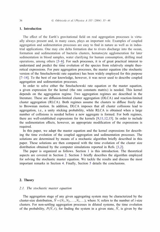
1. Introduction

The e5ect of the Earth’s gravitational #eld on real aggregation processes is virtu-ally always present and, in many cases, plays an important role. Examples of coupledaggregation and sedimentation processes are easy to #nd in nature as well as in indus-trial applications. One may cite delta formation due to rivers discharge into the ocean,formation and sedimentation of bacteria clusters, hematocyte agglomeration for latersedimentation in blood samples, water clarifying for human consumption, drilling mudoperations, among others [3–6]. For such processes, it is of great practical interest tounderstand and predict the time evolution of the species from relatively simple theo-retical expressions. For pure aggregation processes, the master equation (the stochasticversion of the Smoluchowski rate equation) has been widely employed for this purpose[7–14]. To the best of our knowledge, however, it was never used to describe coupledaggregation and sedimentation processes.In order to solve either the Smoluchowski rate equation or the master equation,

a given expression for the kernel (the rate constants matrix) is needed. This kerneldepends on the aggregation regime. Two aggregation regimes are described in theliterature. These are di5usion-limited cluster aggregation (DLCA) and reaction-limitedcluster aggregation (RLCA). Both regimes assume the clusters to di5use freely dueto Brownian motion. In addition, DLCA imposes that all cluster collisions lead toaggregation, i.e., a unity sticking probability, while RLCA is obtained when a largenumber of collisions is needed before a new aggregate is formed. For both regimes,there are well-established expressions for the kernels [9,11,12,15]. In order to includethe sedimentation e5ects, however, an appropriate modi#cation of the expressions isrequired.In this paper, we adapt the master equation and the kernel expressions for describ-

ing the time evolution of the coupled aggregation and sedimentation processes. Thesolutions are determined by means of a stochastic algorithm brieHy described in thispaper. These solutions are then compared with the time evolution of the cluster sizedistribution obtained by the computer simulations reported in Refs. [1,2].The paper is organized as follows. Section 1 is this introduction. The theoretical

aspects are covered in Section 2. Section 3 brieHy describes the algorithm employedfor solving the stochastic master equation. We tackle the results and discuss the mostimportant remarks in Section 4. Finally, Section 5 details the conclusions.

2. Theory

2.1. The stochastic master equation

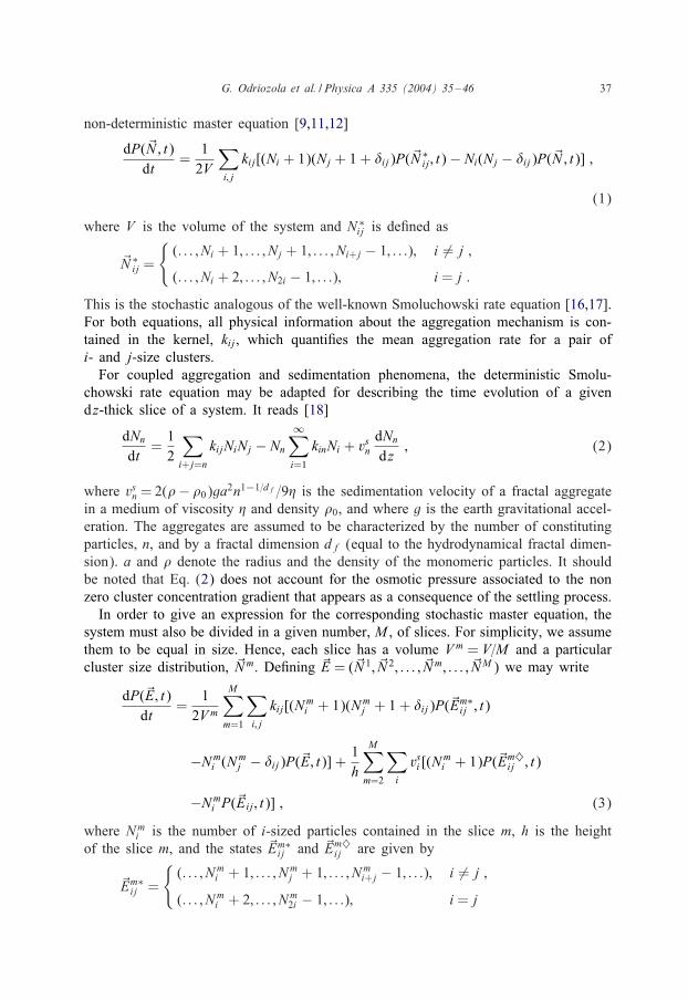
The aggregation stage of any given aggregating system may be characterized by thecluster-size distribution, N=(N1; N2; : : : ; Ni; : : :), where Ni refers to the number of i-sizeclusters. For non-settling aggregation processes in diluted systems, the time evolutionof the probability, P(N ; t), for #nding the system in a given state, N , is given by the

G. Odriozola et al. / Physica A 335 (2004) 35–46 37

non-deterministic master equation [9,11,12]

dP(N ; t)dt

=12V

∑i; j

kij[(Ni + 1)(Nj + 1 + �ij)P(N ∗ij ; t) − Ni(Nj − �ij)P(N ; t)] ;

(1)

where V is the volume of the system and N ∗ij is de#ned as

N ∗ij =

{(: : : ; Ni + 1; : : : ; Nj + 1; : : : ; Ni+j − 1; : : :); i �= j ;

(: : : ; Ni + 2; : : : ; N2i − 1; : : :); i = j :

This is the stochastic analogous of the well-known Smoluchowski rate equation [16,17].For both equations, all physical information about the aggregation mechanism is con-tained in the kernel, kij, which quanti#es the mean aggregation rate for a pair ofi- and j-size clusters.For coupled aggregation and sedimentation phenomena, the deterministic Smolu-

chowski rate equation may be adapted for describing the time evolution of a givendz-thick slice of a system. It reads [18]

dNndt

=12

∑i+j=n

kijNiNj − Nn∞∑i=1

kinNi + vsndNndz

; (2)

where vsn = 2(�− �0)ga2n1−1=df =9� is the sedimentation velocity of a fractal aggregatein a medium of viscosity � and density �0, and where g is the earth gravitational accel-eration. The aggregates are assumed to be characterized by the number of constitutingparticles, n, and by a fractal dimension df (equal to the hydrodynamical fractal dimen-sion). a and � denote the radius and the density of the monomeric particles. It shouldbe noted that Eq. (2) does not account for the osmotic pressure associated to the nonzero cluster concentration gradient that appears as a consequence of the settling process.In order to give an expression for the corresponding stochastic master equation, the

system must also be divided in a given number, M , of slices. For simplicity, we assumethem to be equal in size. Hence, each slice has a volume Vm = V=M and a particularcluster size distribution, Nm. De#ning E = (N 1; N 2; : : : ; N m; : : : ; NM ) we may write

dP(E; t)dt

=1

2Vm

M∑m=1

∑i; j

kij[(Nmi + 1)(Nm

j + 1 + �ij)P(Em∗ij ; t)

−Nmi (N

mj − �ij)P(E; t)] +

1h

M∑m=2

∑i

vsi [(Nmi + 1)P(Em♦

ij ; t)

−Nmi P(Eij ; t)] ; (3)

where Nmi is the number of i-sized particles contained in the slice m, h is the height

of the slice m, and the states Em∗ij and Em♦

ij are given by

Em∗ij =

{(: : : ; Nm

i + 1; : : : ; Nmj + 1; : : : ; Nm

i+j − 1; : : :); i �= j ;

(: : : ; Nmi + 2; : : : ; Nm

2i − 1; : : :); i = j

38 G. Odriozola et al. / Physica A 335 (2004) 35–46

and

Em♦ij = {: : : ; Nm−1

i − 1; : : : ; Nmi + 1; : : : :

Here, the positive term of the #rst sum accounts for aggregation events that allow forthe transition from Em∗

ij towards E. Please note that the state Em∗ij only di5ers form E in

one single aggregation event in the slice m. The negative term of the #rst sum accountsfor those aggregation events that give rise to a transition away from E. The secondsum takes into account the variation of P(E; t) due to mass transfer between the slicesm and m− 1 (arbitrarily, we assign m= 1 to the lower slice and m=M to the upperslice). Hence, a positive term considers those transitions from a state Em♦

ij towards E.Evidently, the only di5erence between Em♦

ij and E is one i-mer in the slice m whichis going to settle towards the next lower slice m− 1. The negative term accounts forthose events that make the system to leave the state E. Since we are considering anisolated system, there is no incoming mass trough the upper boundary and there is nooutgoing mass trough the lower boundary, i.e., the sum limits are imposed as m = 2and M . Finally, it is also necessary to mention that, just like Eq. (2), Eq. (3) does notconsider the osmotic contribution.

2.2. Aggregation kernels

In order to #nd a solution for any of the above-described equations, the aggregationkernel must be known. For DLCA conditions, it is well proved that the Browniankernel yields excellent solutions for the time evolution of the cluster size distribution.It reads [15,19,20]

kBij =kSm114

(i1=df + j1=df)(i−1=df + j−1=df) ; (4)

where kSm11 = 8kT=3� is the Smoluchowski dimer formation rate constant and kT is thethermal energy. This kernel considers all collisions to be e5ective and accounts forBrownian motion as the source of all cluster collisions.For settling particles, however, an additional term must be introduced, as a con-

sequence of the di5erent sedimentation velocities that clusters may have. One maypostulate the following relationship for the Hux of particles j towards a reference par-ticle i [18,21]:

jS = Aij|vsi − vsj |Cj ;where Cj is the j-mer concentration, and Aij is the combined i-j-mer cross-sectionarea. This Hux may be considered equal to the collision frequency between the j-mersand the particular i-mer. For all i-mers the collision frequency becomes

FS = Aij|vsi − vsj |CjCi ;where Ci is the i-mer concentration. Hence, the sedimentation contribution to theaggregation kernel is

kSij = Aij|vsi − vsj | :

G. Odriozola et al. / Physica A 335 (2004) 35–46 39

Assuming Aij = "a2(i1=df + j1=df)2 and introducing the Peclet number, Pe = 4"a4(�−�0)g=3kBT , it #nally reads [19,22,23]

kSij =PekBT6�

(i1=df + j1=df)2|i1−1=df − j1−1=df | : (5)

When not all collisions lead to aggregation, the Brownian kernel has to be modi-#ed in order to account also for the e5ect of non-e5ective collisions. Therefore, thefollowing expression was recently deduced for the kernel [11,12]

kij =P

tdif + (tcij − tdifij )(1 − P)Pcij; (6)

where P is the sticking probability, Pcij is the probability for, given a non-e5ective

collision between an i-mer and a j-mer, the clusters to collide again, tdifij is the averagetime until an i-mer and a j-mer approach due to di5usion, and tcij is the averagetime between two consecutive collisions that i-mers and j-mers may perform. Fornon-settling aggregation, tdifij = (kBrowij )−1 and Eq. (6) becomes

kij =kBijPN11(ij)b

1 + P[N11(ij)b − 1](7)

if one assumes tc�tdif and Nij =N11(ij)b. Here, Nij =∑∞

l=1 lPc(l−1)ij (1 − Pcij) =

1=(1 − Pcij) is the mean number of collisions that two non-aggregating i- and j-mersperform per encounter, N11 is the mean number of collisions per encounter for apair of non-aggregating monomers, and b is a positive constant. For the simulationconditions used in Refs. [11,12], N11 = 6:1 and b= 3:5 were obtained.Considering tdifij = (kBrowij + kSedij )−1 and substituting in Eq. (6), while keeping the

assumptions tc�tdif and Nij =N11(ij)b, one #nally obtains

kij =(kBij + kSij)PN11(ij)b

1 + P[N11(ij)b − 1](8)

for the non-DLCA regime with sedimentation.

3. The stochastic algorithm

For solving Eq. (3) a stochastic simulation approach is employed [7,8]. The pro-cedure involves the calculation of the probability density function, which for pureaggregation processes may be denoted by Pa(); i; j; m) and for pure settling processesit should read Ps(); i; m). For pure aggregation processes, Pa(); i; j; m)d) is the prob-ability that, given the state E at time t, the next reaction in the system will be theaggregation of an i-mer with a j-mer occurring in the slice m during the in#nitesimaltime interval (t + ); t + ) + d)). For pure sedimentation processes, Ps(); i; m) is theprobability that, given the state E at time t, the next reaction in the system will be ani-mer transfer from the slice m+1 to the slice m during the in#nitesimal time interval(t + ); t + )+ d)).

40 G. Odriozola et al. / Physica A 335 (2004) 35–46

De#ning aijm as

aijm =Nmi (N

mj − �ij)kij

Vm(1 + �ij);

the aggregation probability density function for pure aggregation becomes

Pa(); i; j; m) = aijme−a0) ; (9)

where a0 = 12

∑Mm=1

∑Lm

i; j=1 aijm(1 + �ij) and Lm is the size of the largest aggregate inthe slice m. Analogously, for pure sedimentation it is convenient to de#ne

sim =Nmi vih

and hence,

Ps(); i; m) = sime−s0) (10)

is the settling probability density function, where s0 =∑M−1

m=1

∑Lm

i; j=1 sim.The algorithm for calculating the time evolution of the cluster size distribution for

coupled aggregation and sedimentation processes is the following:

(1) Input kij, vi, E(t = 0) and set the time to zero, t = 0.(2) Calculate aijm and sim for all i, j and m. Calculate a0 and s0.(3) Generate the random numbers +1 and +2 uniformly distributed in [0,1].(4) Increment t in )= 1=(a0 + s0)ln(1=+1).(5) If a0¿ +2(a0+s0) then take the #rst m, i and j that veri#es 1

2

∑ml

∑i; jp;q apql(1+

�pq)¿+2(a0 + s0). Consider the reaction as aggregation and adjust the populationof Nm

i+j, Nmi and Nm

j (Nm) accordingly. Continue with the procedure at point 2for recalculating aijm and smi .

(6) Take the #rst m and i that veri#es∑m

l

∑ip spl ¿+2(a0 + s0) − a0. Here, the

reaction is an i-mer transfer from slice m to slice m− 1. Adjust the cluster con-centrations accordingly and continue with the procedure at point 2 for recalculatingaijm and sim.

The procedure ends when a0 + s0 vanishes and so, the whole mass is contained in thesediment.For comparing the solutions of the master equation with the computer simulations

given in Refs. [1,2], the calculations were performed using the same conditions, i.e., asquare section prism with height H=10000a and side L=250a, a monomer particle ra-dius a=315 nm. The solvent was considered to be water at 20◦C. The kernel employedfor the calculations was (8). The prism was divided into M =360 equally sized slices.As will be explained further down in the paper, this choice was not arbitrary. Just asfor the simulations, di5erent Peclet numbers, Pe, and sticking probabilities, P, wereconsidered in order to study their inHuence on the coupled aggregation-sedimentationprocesses. The fractal dimensions, df, were taken from Refs. [1,2] according to thechosen Pe and P. Ten runs were averaged for each set of parameters in order toimprove the statistics of the solutions.

G. Odriozola et al. / Physica A 335 (2004) 35–46 41

4. Results

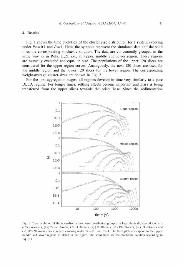
Fig. 1 shows the time evolution of the cluster size distribution for a system evolvingunder Pe=0:1 and P=1. Here, the symbols represent the simulated data and the solidlines the corresponding stochastic solution. The data are conveniently grouped in thesame way as in Refs. [1,2], i.e., an upper, middle and lower region. These regionsare mutually excluded and equal in size. The populations of the upper 120 slices areconsidered for the upper region curves. Analogously, the next 120 slices are used forthe middle region and the lower 120 slices for the lower region. The correspondingweight-average cluster-sizes are shown in Fig. 2.For the #rst aggregation stages, all regions develop in time very similarly to a pure

DLCA regime. For longer times, settling e5ects become important and mass is beingtransferred from the upper slices towards the prism base. Since the sedimentation

10 100 1000 10000

1

1

1E-4

1E-3

0.01

1

Bottom region

(s)

Ni

Middle region

Upper region

time

0.1

0.01

1E-3

1E-4

0.1

0.01

1E-3

1E-4

0.1

Fig. 1. Time evolution of the normalized cluster-size distribution grouped in logarithmically spaced intervals(( ) monomers, (©) 2- and 3-mers, (�) 4–8-mers, (�) 9–18-mers, (♦) 19–38-mers, (+) 39–88-mers and(×) 89–200-mers), for a system evolving under Pe=0:1 and P=1. The three plots correspond to the upper,middle and lower regions as stated in the #gure. The solid lines are the stochastic solution according toEq. (3).

42 G. Odriozola et al. / Physica A 335 (2004) 35–46

1 10 100 1000 10000

1

10

100

Bottom region

Middle region

Upper region

n w

time (s)

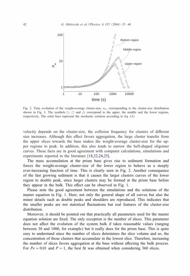
Fig. 2. Time evolution of the weight-average cluster-size, nw , corresponding to the cluster-size distributionshown in Fig. 1. The symbols , © and � correspond to the upper, the middle and the lower regions,respectively. The solid lines represent the stochastic solution according to Eq. (3).

velocity depends on the cluster-size, the collision frequency for clusters of di5erentsize increases. Although this e5ect favors aggregation, the large cluster transfer fromthe upper slices towards the base makes the weight-average cluster-size for the up-per regions to peak. In addition, this also tends to narrow the bell-shaped oligomercurves. These facts are in good agreement with computer calculations, simulations andexperiments reported in the literature [18,22,24,25].The mass accumulation at the prism base gives rise to sediment formation and

forces the weight-average cluster-size of the lower region to behave as a steeplyever-increasing function of time. This is clearly seen in Fig. 2. Another consequenceof the fast growing sediment is that it causes the larger clusters curves of the lowerregion to double peak, since larger clusters may be formed at the prism base beforethey appear in the bulk. This e5ect can be observed in Fig. 1.Please note the good agreement between the simulations and the solutions of the

master equation in Fig. 1. Here, not only the general shape of all curves but also theminor details such as double peaks and shoulders are reproduced. This indicates thatthe smaller peaks are not statistical Huctuations but real features of the cluster-sizedistribution.Moreover, it should be pointed out that practically all parameters used for the master

equation solution are #xed. The only exception is the number of slices. This parameterdoes not a5ect the evolution of the system bulk if takes reasonable values (rangingbetween 30 and 1000, for example) but it really does for the prism base. This is quiteeasy to understand since the number of slices determines the slice volume and so, theconcentration of those clusters that accumulate in the lowest slice. Therefore, increasingthe number of slices favors aggregation at the base without a5ecting the bulk process.For Pe = 0:01 and P = 1, the best #t was obtained when considering 360 slices.

G. Odriozola et al. / Physica A 335 (2004) 35–46 43

10 1000 10000

1

1E-4

1E-3

0.01

1

1

(s)

Ni

Middle region

Upper region0.1

0.01

1E-3

1E-4

0.01

1E-3

1E-4

100time

0.1Bottom region

0.1

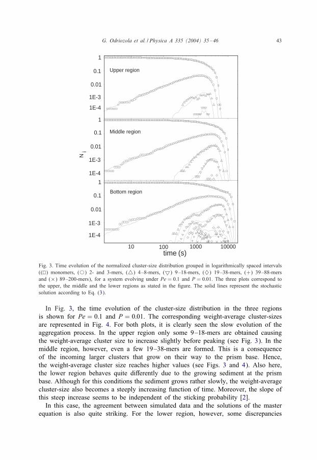
Fig. 3. Time evolution of the normalized cluster-size distribution grouped in logarithmically spaced intervals(( ) monomers, (©) 2- and 3-mers, (�) 4–8-mers, (�) 9–18-mers, (♦) 19–38-mers, (+) 39–88-mersand (×) 89–200-mers), for a system evolving under Pe = 0:1 and P = 0:01. The three plots correspond tothe upper, the middle and the lower regions as stated in the #gure. The solid lines represent the stochasticsolution according to Eq. (3).

In Fig. 3, the time evolution of the cluster-size distribution in the three regionsis shown for Pe = 0:1 and P = 0:01. The corresponding weight-average cluster-sizesare represented in Fig. 4. For both plots, it is clearly seen the slow evolution of theaggregation process. In the upper region only some 9–18-mers are obtained causingthe weight-average cluster size to increase slightly before peaking (see Fig. 3). In themiddle region, however, even a few 19–38-mers are formed. This is a consequenceof the incoming larger clusters that grow on their way to the prism base. Hence,the weight-average cluster size reaches higher values (see Figs. 3 and 4). Also here,the lower region behaves quite di5erently due to the growing sediment at the prismbase. Although for this conditions the sediment grows rather slowly, the weight-averagecluster-size also becomes a steeply increasing function of time. Moreover, the slope ofthis steep increase seems to be independent of the sticking probability [2].In this case, the agreement between simulated data and the solutions of the master

equation is also quite striking. For the lower region, however, some discrepancies

44 G. Odriozola et al. / Physica A 335 (2004) 35–46

1

1

Bottom region

Middle region

Upper region

n w

s)

100

10

100 1000 1000010

time (

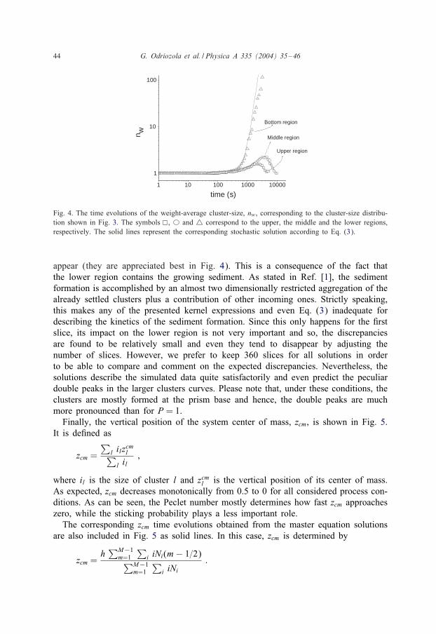
Fig. 4. The time evolutions of the weight-average cluster-size, nw , corresponding to the cluster-size distribu-tion shown in Fig. 3. The symbols , © and � correspond to the upper, the middle and the lower regions,respectively. The solid lines represent the corresponding stochastic solution according to Eq. (3).

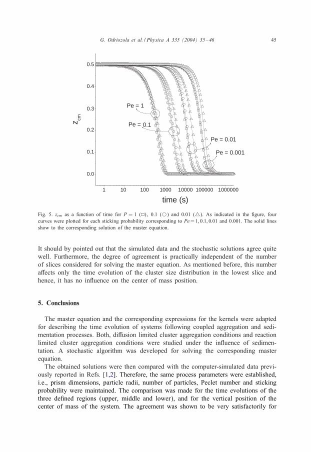
appear (they are appreciated best in Fig. 4). This is a consequence of the fact thatthe lower region contains the growing sediment. As stated in Ref. [1], the sedimentformation is accomplished by an almost two dimensionally restricted aggregation of thealready settled clusters plus a contribution of other incoming ones. Strictly speaking,this makes any of the presented kernel expressions and even Eq. (3) inadequate fordescribing the kinetics of the sediment formation. Since this only happens for the #rstslice, its impact on the lower region is not very important and so, the discrepanciesare found to be relatively small and even they tend to disappear by adjusting thenumber of slices. However, we prefer to keep 360 slices for all solutions in orderto be able to compare and comment on the expected discrepancies. Nevertheless, thesolutions describe the simulated data quite satisfactorily and even predict the peculiardouble peaks in the larger clusters curves. Please note that, under these conditions, theclusters are mostly formed at the prism base and hence, the double peaks are muchmore pronounced than for P = 1.Finally, the vertical position of the system center of mass, zcm, is shown in Fig. 5.

It is de#ned as

zcm =∑

l ilzcml∑

l il;

where il is the size of cluster l and zcml is the vertical position of its center of mass.As expected, zcm decreases monotonically from 0.5 to 0 for all considered process con-ditions. As can be seen, the Peclet number mostly determines how fast zcm approacheszero, while the sticking probability plays a less important role.The corresponding zcm time evolutions obtained from the master equation solutions

are also included in Fig. 5 as solid lines. In this case, zcm is determined by

zcm =h

∑M−1m=1

∑i iNi(m− 1=2)∑M−1

m=1

∑i iNi

:

G. Odriozola et al. / Physica A 335 (2004) 35–46 45

1 100

0.0

0.4

0.5

Pe = 0.001

Pe = 0.01

Pe =

Pe = 1

z cm

time (s)

0.2

0.3

0.1

1000 10000 100000 100000010

0.1

Fig. 5. zcm as a function of time for P = 1 ( ) , 0.1 (©) and 0.01 (�). As indicated in the #gure, fourcurves were plotted for each sticking probability corresponding to Pe=1; 0:1; 0:01 and 0.001. The solid linesshow to the corresponding solution of the master equation.

It should by pointed out that the simulated data and the stochastic solutions agree quitewell. Furthermore, the degree of agreement is practically independent of the numberof slices considered for solving the master equation. As mentioned before, this numbera5ects only the time evolution of the cluster size distribution in the lowest slice andhence, it has no inHuence on the center of mass position.

5. Conclusions

The master equation and the corresponding expressions for the kernels were adaptedfor describing the time evolution of systems following coupled aggregation and sedi-mentation processes. Both, di5usion limited cluster aggregation conditions and reactionlimited cluster aggregation conditions were studied under the inHuence of sedimen-tation. A stochastic algorithm was developed for solving the corresponding masterequation.The obtained solutions were then compared with the computer-simulated data previ-

ously reported in Refs. [1,2]. Therefore, the same process parameters were established,i.e., prism dimensions, particle radii, number of particles, Peclet number and stickingprobability were maintained. The comparison was made for the time evolutions of thethree de#ned regions (upper, middle and lower), and for the vertical position of thecenter of mass of the system. The agreement was shown to be very satisfactorily for

46 G. Odriozola et al. / Physica A 335 (2004) 35–46

the bulk but some expected di5erences appeared for the prism base, where the sedimentgrows.

Acknowledgements

This work was supported by the Instituto Mexicano del Petr.oleo grant D.00072.A.S. and R.H-A. thank the “Ministerio de Ciencia y Tecnolog.Na, Plan Nacional deInvestigaci.on, Desarrollo e Innovaci.on Tecnol.ogica (I+D+I) Project N ◦MAT2000–1550–C03–01” for the #nancial support.

References

[1] R. Leone, G. Odriozola, L. Mussio, A. Schmitt, R. Hidalgo- .Alvarez, Eur. Phys. J. E 7 (2002) 105.[2] G. Odriozola, R. Leone, A. Schmitt, A. Moncho-Jorda, R. Hidalgo- .Alvarez, Phys. Rev. E 65 (2003)

031405.[3] J. Lyklema, Fundamentals of Interface and Colloid Science, Vol. I, Fundamentals, Academic Press,

London, 1991.[4] F. Family, D.P. Landau, Kinetics of Aggregation and Gelation, North-Holland, Amsterdam, 1984.[5] R.J. Hunter, Foundations of Colloid Science, Clarendon Press, Oxford, 1987.[6] H. Van Olphen, An Introduction to Clay Colloid Chemistry, Interscience, London, 1977.[7] D.T. Gillespie, J. Comput. Phys. 22 (1976) 403.[8] D.T. Gillespie, J. Phys. Chem. 81 (1977) 2340.[9] M. Thorn, M.L. Broide, M. Seesselberg, Phys. Rev. Lett. 72 (1994) 3622.[10] M. Thorn, M. Seesselberg, Phys. Rev. E 51 (1995) 4089.[11] G. Odriozola, A. Moncho-Jord.a, A. Schmitt, J. Callejas-Fern.andez, R. Mart.Nnez-Garc.Na, R. Hidalgo-

.Alvarez, Europhys. Lett. 53 (2001) 797.[12] A. Moncho-Jord.a, G. Odriozola, F. Mart.Nnez-L.opez, A. Schmitt, R. Hidalgo- .Alvarez, Eur. Phys. J. E

5 (2001) 471.[13] G. Odriozola, A. Schmitt, A. Moncho-Jord.a, J. Callejas-Fern.andez, R. Mart.Nnez-Garc.Na, R. Leone,

R. Hidalgo- .Alvarez, Phys. Rev. E 65 (2001) 031405.[14] G. Odriozola, A. Schmitt, J. Callejas-Fern.andez, R. Mart.Nnez-Garc.Na, R. Leone, R. Hidalgo- .Alvarez,

J. Phys. Chem. B 107 (2002) 2180.[15] M.L. Broide, R.J. Cohen, Phys. Rev. Lett. 64 (1990) 2026.[16] M. von Smoluchowski, Phys. Z 17 (1916) 557.[17] M. von Smoluchowski, Z. Phys. Chem. 92 (1917) 129.[18] S.B. Grant, J.H. Kimm, C. Poor, J. Colloid Interface Sci. 238 (2001) 238.[19] M. Lattuada, P. SandkRuhler, H. Wu, J. Sefcik, M. Morbidelli, Adv. Colloid Interface Sci. 103 (2003)

33.[20] P. SandkRuhler, J. Sefcik, M. Lattuada, H. Wu, M. Morbidelli, A.l.Ch.E. J. 49 (2003) 1542.[21] A. Thill, S. Moustier, J. Aziz, M.R. Wiesner, Y. Bottero, J. Colloid Interface Sci. 243 (2001) 171.[22] H. Wu, M. Lattuada, P. SandkRuhler, J. Sefcik, M. Morbidelli, Langmuir (2004), to be published.[23] S.K. Friedlander, Smoke, Dust and Haze, Wiley-Interscience, New York, 1977.[24] A.E. Gonzalez, Phys. Rev. Lett. 86 (2001) 1243.[25] C. Allain, M. Cloitre, M. Wafra, Phys. Rev. Lett. 74 (1995) 1478.