Numerical simulations of particle sedimentation using the immersed boundary method
Upload
khangminh22Category
view
1download
0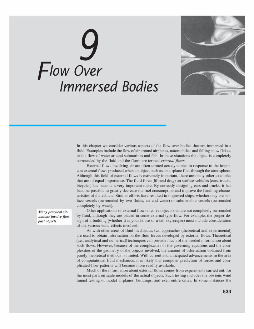
In this chapter we consider various aspects of the flow over bodies that are immersed in a
fluid. Examples include the flow of air around airplanes, automobiles, and falling snow flakes,
or the flow of water around submarines and fish. In these situations the object is completely
surrounded by the fluid and the flows are termed external flows.
External flows involving air are often termed aerodynamics in response to the impor-
tant external flows produced when an object such as an airplane flies through the atmosphere.
Although this field of external flows is extremely important, there are many other examples
that are of equal importance. The fluid force 1lift and drag2 on surface vehicles 1cars, trucks,
bicycles2 has become a very important topic. By correctly designing cars and trucks, it has
become possible to greatly decrease the fuel consumption and improve the handling charac-
teristics of the vehicle. Similar efforts have resulted in improved ships, whether they are sur-
face vessels 1surrounded by two fluids, air and water2 or submersible vessels 1surrounded
completely by water2.Other applications of external flows involve objects that are not completely surrounded
by fluid, although they are placed in some external-type flow. For example, the proper de-
sign of a building 1whether it is your house or a tall skyscraper2 must include consideration
of the various wind effects involved.
As with other areas of fluid mechanics, two approaches 1theoretical and experimental2are used to obtain information on the fluid forces developed by external flows. Theoretical
1i.e., analytical and numerical2 techniques can provide much of the needed information about
such flows. However, because of the complexities of the governing equations and the com-
plexities of the geometry of the objects involved, the amount of information obtained from
purely theoretical methods is limited. With current and anticipated advancements in the area
of computational fluid mechanics, it is likely that computer prediction of forces and com-
plicated flow patterns will become more readily available.
Much of the information about external flows comes from experiments carried out, for
the most part, on scale models of the actual objects. Such testing includes the obvious wind
tunnel testing of model airplanes, buildings, and even entire cities. In some instances the
533
9Flow Over
Immersed Bodies
Many practical sit-
uations involve flow
past objects.

actual device, not a model, is tested in wind tunnels. Figure 9.1 shows tests of vehicles in
wind tunnels. Better performance of cars, bikes, skiers, and numerous other objects has re-
sulted from testing in wind tunnels. The use of water tunnels and towing tanks also provides
useful information about the flow around ships and other objects.
In this chapter we consider characteristics of external flow past a variety of objects.
We investigate the qualitative aspects of such flows and learn how to determine the various
forces on objects surrounded by a moving liquid.
534 ■ Chapter 9 / Flow Over Immersed Bodies
9.1 General External Flow Characteristics
A body immersed in a moving fluid experiences a resultant force due to the interaction be-
tween the body and the fluid surrounding it. In some instances 1such as an airplane flying
through still air2 the fluid far from the body is stationary and the body moves through the
fluid with velocity U. In other instances 1such as the wind blowing past a building2 the body
is stationary and the fluid flows past the body with velocity U. In any case, we can fix the
coordinate system in the body and treat the situation as fluid flowing past a stationary body
For external flows
it is usually easiest
to use a coordinate
system fixed to the
object.
■ F I G U R E 9 . 1
(a) Flow past a full-sized streamlined ve-hicle in the GM aero-dynamics laboratorywind tunnel, an 18-ftby 34-ft test sectionfacility driven by a4000-hp, 43-ft-diame-ter fan. (Photographcourtesy of GeneralMotors Corporation.)(b) Surface flow on amodel vehicle as indi-cated by tufts at-tached to the surface.(Reprinted with per-mission from Societyof Automotive Engi-neers, Ref. 28.)
with velocity U, the upstream velocity. For the purposes of this book, we will assume that
the upstream velocity is constant in both time and location. That is, there is a uniform, con-
stant velocity fluid flowing past the object. In actual situations this is often not true. For ex-
ample, the wind blowing past a smokestack is nearly always turbulent and gusty 1unsteady2and probably not of uniform velocity from the top to the bottom of the stack. Usually the
unsteadiness and nonuniformity are of minor importance.
Even with a steady, uniform upstream flow, the flow in the vicinity of an object may
be unsteady. Examples of this type of behavior include the flutter that is sometimes found
in the flow past airfoils 1wings2, the regular oscillation of telephone wires that “sing” in a
wind, and the irregular turbulent fluctuations in the wake regions behind bodies.
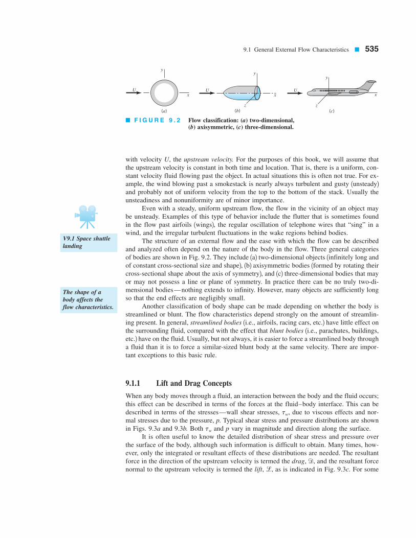
The structure of an external flow and the ease with which the flow can be described
and analyzed often depend on the nature of the body in the flow. Three general categories
of bodies are shown in Fig. 9.2. They include 1a2 two-dimensional objects 1infinitely long and
of constant cross-sectional size and shape2, 1b2 axisymmetric bodies 1formed by rotating their
cross-sectional shape about the axis of symmetry2, and 1c2 three-dimensional bodies that may
or may not possess a line or plane of symmetry. In practice there can be no truly two-di-
mensional bodies—nothing extends to infinity. However, many objects are sufficiently long
so that the end effects are negligibly small.
Another classification of body shape can be made depending on whether the body is
streamlined or blunt. The flow characteristics depend strongly on the amount of streamlin-
ing present. In general, streamlined bodies 1i.e., airfoils, racing cars, etc.2 have little effect on
the surrounding fluid, compared with the effect that blunt bodies 1i.e., parachutes, buildings,
etc.2 have on the fluid. Usually, but not always, it is easier to force a streamlined body through
a fluid than it is to force a similar-sized blunt body at the same velocity. There are impor-
tant exceptions to this basic rule.
9.1.1 Lift and Drag Concepts
When any body moves through a fluid, an interaction between the body and the fluid occurs;
this effect can be described in terms of the forces at the fluid–body interface. This can be
described in terms of the stresses—wall shear stresses, due to viscous effects and nor-
mal stresses due to the pressure, p. Typical shear stress and pressure distributions are shown
in Figs. 9.3a and 9.3b. Both and p vary in magnitude and direction along the surface.
It is often useful to know the detailed distribution of shear stress and pressure over
the surface of the body, although such information is difficult to obtain. Many times, how-
ever, only the integrated or resultant effects of these distributions are needed. The resultant
force in the direction of the upstream velocity is termed the drag, and the resultant force
normal to the upstream velocity is termed the lift, as is indicated in Fig. 9.3c. For somel,
d,
tw
tw,
9.1 General External Flow Characteristics ■ 535
U U Ux
z
y
z
y
xx
y
(c)(b)(a)
■ F I G U R E 9 . 2 Flow classification: (a) two-dimensional,(b) axisymmetric, (c) three-dimensional.
V9.1 Space shuttle
landing
The shape of a
body affects the
flow characteristics.
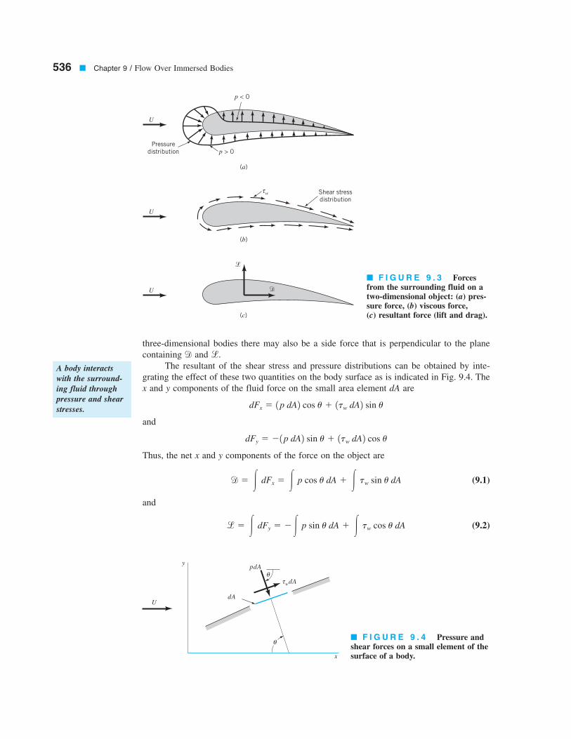
three-dimensional bodies there may also be a side force that is perpendicular to the plane
containing and
The resultant of the shear stress and pressure distributions can be obtained by inte-
grating the effect of these two quantities on the body surface as is indicated in Fig. 9.4. The
x and y components of the fluid force on the small area element dA are
and
Thus, the net x and y components of the force on the object are
(9.1)
and
(9.2) l 5 # dFy 5 2# p sin u dA 1 # tw cos u dA
d 5 # dFx 5 # p cos u dA 1 # tw sin u dA
dFy 5 21p dA2 sin u 1 1tw dA2 cos u
dFx 5 1p dA2 cos u 1 1tw dA2 sin u
l.d
536 ■ Chapter 9 / Flow Over Immersed Bodies
A body interacts
with the surround-
ing fluid through
pressure and shear
stresses.
■ F I G U R E 9 . 3 Forcesfrom the surrounding fluid on atwo-dimensional object: (a) pres-sure force, (b) viscous force,(c) resultant force (lift and drag).
■ F I G U R E 9 . 4 Pressure andshear forces on a small element of thesurface of a body.
U
U
U $
+
(c)
(b)
(a)
w Shear stress
distribution
τ
p > 0
Pressure
distribution
p < 0
U
pdA
θ
dA
τwdA
θ
y
x
Of course, to carry out the integrations and determine the lift and drag, we must know the
body shape 1i.e., as a function of location along the body2 and the distribution of and p
along the surface. These distributions are often extremely difficult to obtain, either experi-
mentally or theoretically. The pressure distribution can be obtained experimentally without
too much difficulty by use of a series of static pressure taps along the body surface. On the
other hand, it is usually quite difficult to measure the wall shear stress distribution.
It is seen that both the shear stress and pressure force contribute to the lift and drag,
since for an arbitrary body is neither zero nor along the entire body. The exception is
a flat plate aligned either parallel to the upstream flow or normal to the upstream
flow as is discussed in Example 9.1.1u 5 021u 5 90°2
90°u
twu
9.1 General External Flow Characteristics ■ 537
EXAMPLE
9.1
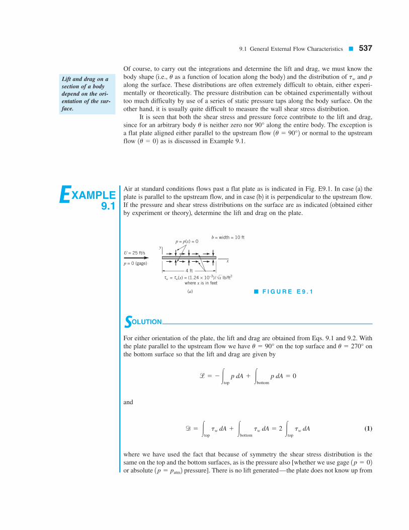
Air at standard conditions flows past a flat plate as is indicated in Fig. E9.1. In case 1a2 the
plate is parallel to the upstream flow, and in case 1b2 it is perpendicular to the upstream flow.
If the pressure and shear stress distributions on the surface are as indicated 1obtained either
by experiment or theory2, determine the lift and drag on the plate.
Lift and drag on a
section of a body
depend on the ori-
entation of the sur-
face.
SOLUTION
For either orientation of the plate, the lift and drag are obtained from Eqs. 9.1 and 9.2. With
the plate parallel to the upstream flow we have on the top surface and on
the bottom surface so that the lift and drag are given by
and
(1)
where we have used the fact that because of symmetry the shear stress distribution is the
same on the top and the bottom surfaces, as is the pressure also [whether we use gage
or absolute pressure]. There is no lift generated—the plate does not know up from1 p 5 patm21 p 5 02
d 5 #top
tw dA 1 #bottom
tw dA 5 2 #top
tw dA
l 5 2#top
p dA 1 #bottom
p dA 5 0
u 5 270°u 5 90°
U = 25 ft/s
p = 0 (gage)
y
x
p = p(x) = 0
4 ft
b = width = 10 ft
= (x) = (1.24 × 10⁻³)/ x lb/ft2
where x is in feet
√τ
(a)
w τw
■ F I G U R E E 9 . 1

538 ■ Chapter 9 / Flow Over Immersed Bodies
down. With the given shear stress distribution, Eq. 1 gives
or
(Ans)
With the plate perpendicular to the upstream flow, we have on the front and
on the back. Thus, from Eqs. 9.1 and 9.2
and
Again there is no lift because the pressure forces act parallel to the upstream flow 1in the di-
rection of not 2 and the shear stress is symmetrical about the center of the plate. With
the given relatively large pressure on the front of the plate 1the center of the plate is a stag-
nation point2 and the negative pressure 1less than the upstream pressure2 on the back of the
plate, we obtain the following drag
or
(Ans)
Clearly there are two mechanisms responsible for the drag. On the ultimately stream-
lined body 1a zero thickness flat plate parallel to the flow2 the drag is entirely due to the shear
stress at the surface and, in this example, is relatively small. For the ultimately blunted body
d 5 55.6 lb
d 5 #2 ft
y522
c0.744 a1 2y
2
4b lb/ft
22 120.8932 lb/ft
2 d 110 ft2 dy
ld
d 5 #front
p dA 2 #back
p dA
l 5 #front
tw dA 2 #back
tw dA 5 0
u 5 180°
u 5 0°
d 5 0.0992 lb
d 5 2 #4 ft
x50
a1.24 3 1023
x1/2 lb/ft
2b 110 ft2 dx
U = 25 ft/s
U
Low p
High p
+ ≠ 0
$ ≠ 0
(c)(b)
p = 0
p = 0.744 1 – lb/ft2
where y is in feet
y2__4
y
p = –0.893 lb/ft2
x
(y) =
– (–y)
( )
τw
τwτw
τw
τw
■ F I G U R E E 9 . 1 (Continued)
9.1 General External Flow Characteristics ■ 539
1a flat plate normal to the upstream flow2 the drag is entirely due to the pressure difference
between the front and back portions of the object and, in this example, is relatively large.
If the flat plate were oriented at an arbitrary angle relative to the upstream flow as in-
dicated in Fig. E9.1c, there would be both a lift and a drag, each of which would be depen-
dent on both the shear stress and the pressure. Both the pressure and shear stress distribu-
tions would be different for the top and bottom surfaces.
Although Eqs. 9.1 and 9.2 are valid for any body, the difficulty in their use lies in ob-
taining the appropriate shear stress and pressure distributions on the body surface. Consid-
erable effort has gone into determining these quantities, but because of the various com-
plexities involved, such information is available only for certain simple situations.
Without detailed information concerning the shear stress and pressure distributions on
a body, Eqs. 9.1 and 9.2 cannot be used. The widely used alternative is to define dimen-
sionless lift and drag coefficients and determine their approximate values by means of either
a simplified analysis, some numerical technique, or an appropriate experiment. The lift co-
efficient, and drag coefficient, are defined as
and
where A is a characteristic area of the object 1see Chapter 72. Typically, A is taken to be frontal
area—the projected area seen by a person looking toward the object from a direction par-
allel to the upstream velocity, U. It would be the area of the shadow of the object projected
onto a screen normal to the upstream velocity as formed by a light shining along the up-
stream flow. In other situations A is taken to be the planform area—the projected area seen
by an observer looking toward the object from a direction normal to the upstream velocity
1i.e., from “above” it2. Obviously, which characteristic area is used in the definition of the
lift and drag coefficients must be clearly stated.
9.1.2 Characteristics of Flow Past an Object
External flows past objects encompass an extremely wide variety of fluid mechanics phe-
nomena. Clearly the character of the flow field is a function of the shape of the body. Flows
past relatively simple geometric shapes 1i.e., a sphere or circular cylinder2 are expected to
have less complex flow fields than flows past a complex shape such as an airplane or a tree.
However, even the simplest-shaped objects produce rather complex flows.
For a given-shaped object, the characteristics of the flow depend very strongly on
various parameters such as size, orientation, speed, and fluid properties. As is discussed in
Chapter 7, according to dimensional analysis arguments, the character of the flow should
depend on the various dimensionless parameters involved. For typical external flows the most
important of these parameters are the Reynolds number, the Mach
number, and for flows with a free surface 1i.e., flows with an interface between
two fluids, such as the flow past a surface ship2, the Froude number, 1Recall
that is some characteristic length of the object and c is the speed of sound.2For the present, we consider how the external flow and its associated lift and drag vary
as a function of Reynolds number. Recall that the Reynolds number represents the ratio of
/
Fr 5 U/1g/.
Ma 5 U/c,
Re 5 rU//m 5 U//n,
CD 5d
12rU
2A
CL 5l
12rU
2A
CD,CL,
Lift coefficients and
drag coefficients
are dimensionless
forms of lift and
drag.

inertial effects to viscous effects. In the absence of all viscous effects the Reynolds
number is infinite. On the other hand, in the absence of all inertial effects 1negligible mass
or 2, the Reynolds number is zero. Clearly, any actual flow will have a Reynolds num-
ber between 1but not including2 these two extremes. The nature of the flow past a body de-
pends strongly on whether or
Most external flows with which we are familiar are associated with moderately sized
objects with a characteristic length on the order of In addition, typi-
cal upstream velocities are on the order of and the fluids involved
are typically water or air. The resulting Reynolds number range for such flows is approxi-
mately As a rule of thumb, flows with are dominated by iner-
tial effects, whereas flows with are dominated by viscous effects. Hence, most fa-
miliar external flows are dominated by inertia.
On the other hand, there are many external flows in which the Reynolds number is
considerably less than 1, indicating in some sense that viscous forces are more important
than inertial forces. The gradual settling of small particles of dirt in a lake or stream is gov-
erned by low Reynolds number flow principles because of the small diameter of the parti-
cles and their small settling speed. Similarly, the Reynolds number for objects moving through
large viscosity oils is small because is large. The general differences between small and
large Reynolds number flow past streamlined and blunt objects can be illustrated by con-
sidering flows past two objects—one a flat plate parallel to the upstream velocity and the
other a circular cylinder.
Flows past three flat plates of length with and are shown
in Fig. 9.5. If the Reynolds number is small, the viscous effects are relatively strong and the
plate affects the uniform upstream flow far ahead, above, below, and behind the plate. To
reach that portion of the flow field where the velocity has been altered by less than 1% of
its undisturbed value we must travel relatively far from the plate. In
low Reynolds number flows the viscous effects are felt far from the object in all directions.
As the Reynolds number is increased 1by increasing U, for example2, the region in
which viscous effects are important becomes smaller in all directions except downstream, as
is shown in Fig. 9.5b. One does not need to travel very far ahead, above, or below the plate
to reach areas in which the viscous effects of the plate are not felt. The streamlines are dis-
placed from their original uniform upstream conditions, but the displacement is not as great
as for the situation shown in Fig. 9.5a.
If the Reynolds number is large 1but not infinite2, the flow is dominated by inertial ef-
fects and the viscous effects are negligible everywhere except in a region very close to the
plate and in the relatively thin wake region behind the plate, as shown in Fig. 9.5c. Since the
fluid viscosity is not zero it follows that the fluid must stick to the solid surface
1the no-slip boundary condition2. There is a thin boundary layer region of thickness
1i.e., thin relative to the length of the plate2 next to the plate in which the fluid
velocity changes from the upstream value of to zero velocity on the plate. The thick-
ness of this layer increases in the direction of flow, starting from zero at the forward or lead-
ing edge of the plate. The flow within the boundary layer may be laminar or turbulent, de-
pending on various parameters involved.
The streamlines of the flow outside of the boundary layer are nearly parallel to the
plate. As we will see in the next section, the slight displacement of the external streamlines
that are outside of the boundary layer is due to the thickening of the boundary layer in the
direction of flow. The existence of the plate has very little effect on the streamlines outside
of the boundary layer—either ahead, above, or below the plate. On the other hand, the wake
region is due entirely to the viscous interaction between the fluid and the plate.
One of the great advancements in fluid mechanics occurred in 1904 as a result of the
insight of Ludwig Prandtl 11875–19532, a German physicist and aerodynamicist. He con-
u 5 U
d 5 d 1x2 ! /
1Re 6 ` 2,
Re 5 0.1
1i.e., U 2 u 6 0.01 U2
107Re 5 rU//m 5 0.1, 10,/
m
Re 6 1
Re 7 10010 6 Re 6 109.
0.01 m/s 6 U 6 100 m/s
0.01 m 6 / 6 10 m.
Re ! 1.Re @ 1
r 5 0
1m 5 02,
540 ■ Chapter 9 / Flow Over Immersed Bodies
The character of
flow past an object
is dependent on the
value of the
Reynolds number.

ceived of the idea of the boundary layer—a thin region on the surface of a body in which
viscous effects are very important and outside of which the fluid behaves essentially as if it
were inviscid. Clearly the actual fluid viscosity is the same throughout; only the relative im-
portance of the viscous effects 1due to the velocity gradients2 is different within or outside
of the boundary layer. As is discussed in the next section, by using such a hypothesis it is
possible to simplify the analysis of large Reynolds number flows, thereby allowing solution
to external flow problems that are otherwise still unsolvable.
As with the flow past the flat plate described above, the flow past a blunt object 1such
as a circular cylinder2 also varies with Reynolds number. In general, the larger the Reynolds
number, the smaller the region of the flow field in which viscous effects are important. For
9.1 General External Flow Characteristics ■ 541
Thin boundary lay-
ers may develop in
large Reynolds
number flows.
Streamlines deflectedconsiderably
Re = U,/v = 0.1
U
Viscous effectsimportant
u < 0.99U
y
x
U
(a)
U
u < 0.99U
y
x
Viscous effectsimportant
Streamlines deflectedsomewhat
Re = 10
Viscosity notimportant
U
Viscosity notimportant
Re = 107
(b)
U
(c)
Viscous effectsimportant
Boundary layer
y
Streamlines deflectionvery slight
δ << ,
Wakeregion
U
x
,
■ F I G U R E 9 . 5
Character of the steady,viscous flow past a flatplate parallel to the up-stream velocity: (a) lowReynolds number flow,(b) moderate Reynoldsnumber flow, (c) largeReynolds number flow.

objects that are not sufficiently streamlined, however, an additional characteristic of the flow
is observed. This is termed flow separation and is illustrated in Fig. 9.6.
Low Reynolds number flow past a circular cylinder is character-
ized by the fact that the presence of the cylinder and the accompanying viscous effects are
felt throughout a relatively large portion of the flow field. As is indicated in Fig. 9.6a, for
the viscous effects are important several diameters in any direction from
the cylinder. A somewhat surprising characteristic of this flow is that the streamlines are es-
sentially symmetric about the center of the cylinder—the streamline pattern is the same in
front of the cylinder as it is behind the cylinder.
As the Reynolds number is increased, the region ahead of the cylinder in which vis-
cous effects are important becomes smaller, with the viscous region extending only a short
distance ahead of the cylinder. The viscous effects are convected downstream and the flow
loses its symmetry. Another characteristic of external flows becomes important—the flow
separates from the body at the separation location as indicated in Fig. 9.6b. With the increase
in Reynolds number, the fluid inertia becomes more important and at some location on the
body, denoted the separation location, the fluid’s inertia is such that it cannot follow the
curved path around to the rear of the body. The result is a separation bubble behind the cylin-
der in which some of the fluid is actually flowing upstream, against the direction of the up-
stream flow. (See the photograph at the beginning of Chapter 9.)
At still larger Reynolds numbers, the area affected by the viscous forces is forced far-
ther downstream until it involves only a thin boundary layer on the front portion of1d ! D2
Re 5 UD/n 5 0.1,
1Re 5 UD/n 6 12
542 ■ Chapter 9 / Flow Over Immersed Bodies
Flow separation
may occur behind
blunt objects.
U
U
U
(c)
(b)
(a)
D
D
Boundary layer
Separated region
Viscosity not
important
Re = 105
δ <<D
Boundary layer separation
Viscous effects
important
Wake
region
x
Separation bubble
Separationlocation
Viscosity not
important
Re = 50
Viscous forces
important throughout
Re = UD/v = 0.1
x
x
Viscous
effects
important
■ F I G U R E 9 . 6
Character of thesteady, viscous flowpast a circular cylin-der: (a) low Reynoldsnumber flow,(b) moderate Rey-nolds number flow,(c) large Reynoldsnumber flow.

the cylinder and an irregular, unsteady 1perhaps turbulent2 wake region that extends far down-
stream of the cylinder. The fluid in the region outside of the boundary layer and wake region
flows as if it were inviscid. Of course, the fluid viscosity is the same throughout the entire
flow field. Whether viscous effects are important or not depends on which region of the flow
field we consider. The velocity gradients within the boundary layer and wake regions are
much larger than those in the remainder of the flow field. Since the shear stress 1i.e., viscous
effect2 is the product of the fluid viscosity and the velocity gradient, it follows that viscous
effects are confined to the boundary layer and wake regions.
The characteristics described in Figs. 9.5 and 9.6 for flow past a flat plate and a circular
cylinder are typical of flows past streamlined and blunt bodies, respectively. The nature of the
flow depends strongly on the Reynolds number. (See Ref. 31 for many examples illustrating
this behavior.) Most familiar flows are similar to the large Reynolds number flows depicted in
Figs. 9.5c and 9.6c, rather than the low Reynolds number flow situations. (See the photograph
at the beginning of Chapters 7 and 11.) In the remainder of this chapter we will investigate
more thoroughly these ideas and determine how to calculate the forces on immersed bodies.
9.1 General External Flow Characteristics ■ 543
Most familiar flows
involve large
Reynolds numbers.
V9.2 Streamlined
and blunt bodies
EXAMPLE
9.2
Reynolds (a) Model in (b) Model inNumber Glycerin Air (c) Car in Air
0.571 46.6
0.672 54.8
1.68 137.0 8.56 3 106Re/
3.42 3 106Reb
2.91 3 106Reh
It is desired to determine the various characteristics of flow past a car. The following tests
could be carried out: 1a2 flow of glycerin past a scale model that is 34-mm
tall, 100-mm long and 40-mm wide, 1b2 air flow past the scale model, or
1c2 air flow past the actual car, which is 1.7-m tall, 5-m long, and 2-m wide.
Would the flow characteristics for these three situations be similar? Explain.
SOLUTION
The characteristics of flow past an object depend on the Reynolds number. For this instance
we could pick the characteristic length to be the height, h, width, b, or length, of the car
to obtain three possible Reynolds numbers, and
These numbers will be different because of the different values of h, b, and Once we ar-
bitrarily decide on the length we wish to use as the characteristic length, we must stick with
it for all calculations when using comparisons between model and prototype.
With the values of kinematic viscosity for air and glycerin obtained from Tables 1.8
and 1.6 as and we obtain the follow-
ing Reynolds numbers for the flows described.
Clearly, the Reynolds numbers for the three flows are quite different 1regardless of
which characteristic length we choose2. Based on the previous discussion concerning flow
past a flat plate or flow past a circular cylinder, we would expect that the flow past the ac-
tual car would behave in some way similar to the flows shown in Figs. 9.5c or 9.6c. That is,
we would expect some type of boundary layer characteristic in which viscous effects would
be confined to relatively thin layers near the surface of the car and the wake region behind
it. Whether the car would act more like a flat plate or a cylinder would depend on the amount
of streamlining incorporated into the car’s design.
nglycerin 5 1.19 3 1023 m2/s,nair 5 1.46 3 1025 m2
/s
/.
Re/ 5 U//n.Reh 5 Uh/n, Reb 5 Ub/n,
/,
U 5 25 m/s
U 5 20 mm/s
U 5 20 mm/s
9.2 Boundary Layer Characteristics
544 ■ Chapter 9 / Flow Over Immersed Bodies
Because of the small Reynolds number involved, the flow past the model car in glyc-
erin would be dominated by viscous effects, in some way reminiscent of the flows depicted
in Figs. 9.5a or 9.6a. Similarly, with the moderate Reynolds number involved for the air flow
past the model, a flow with characteristics similar to those indicated in Figs. 9.5b and 9.6b
would be expected. Viscous effects would be important—not as important as with the glyc-
erin flow, but more important than with the full-sized car.
It would not be a wise decision to expect the flow past the full-sized car to be similar
to the flow past either of the models. The same conclusions result regardless of whether we
use or As is indicated in Chapter 7, the flows past the model car and the full-
sized prototype will not be similar unless the Reynolds numbers for the model and proto-
type are the same. It is not always an easy task to ensure this condition. One 1expensive2 so-
lution is to test full-sized prototypes in very large wind tunnels 1see Fig. 9.12.
Re/.Reh, Reb,
As was discussed in the previous section, it is often possible to treat flow past an object as
a combination of viscous flow in the boundary layer and inviscid flow elsewhere. If the
Reynolds number is large enough, viscous effects are important only in the boundary layer
regions near the object 1and in the wake region behind the object2. The boundary layer is
needed to allow for the no-slip boundary condition that requires the fluid to cling to any solid
surface that it flows past. Outside of the boundary layer the velocity gradients normal to the
flow are relatively small, and the fluid acts as if it were inviscid, even though the viscosity
is not zero. A necessary condition for this structure of the flow is that the Reynolds number
be large.
9.2.1 Boundary Layer Structure and Thickness on a Flat Plate
There can be a wide variety in the size of a boundary layer and the structure of the flow
within it. Part of this variation is due to the shape of the object on which the boundary layer
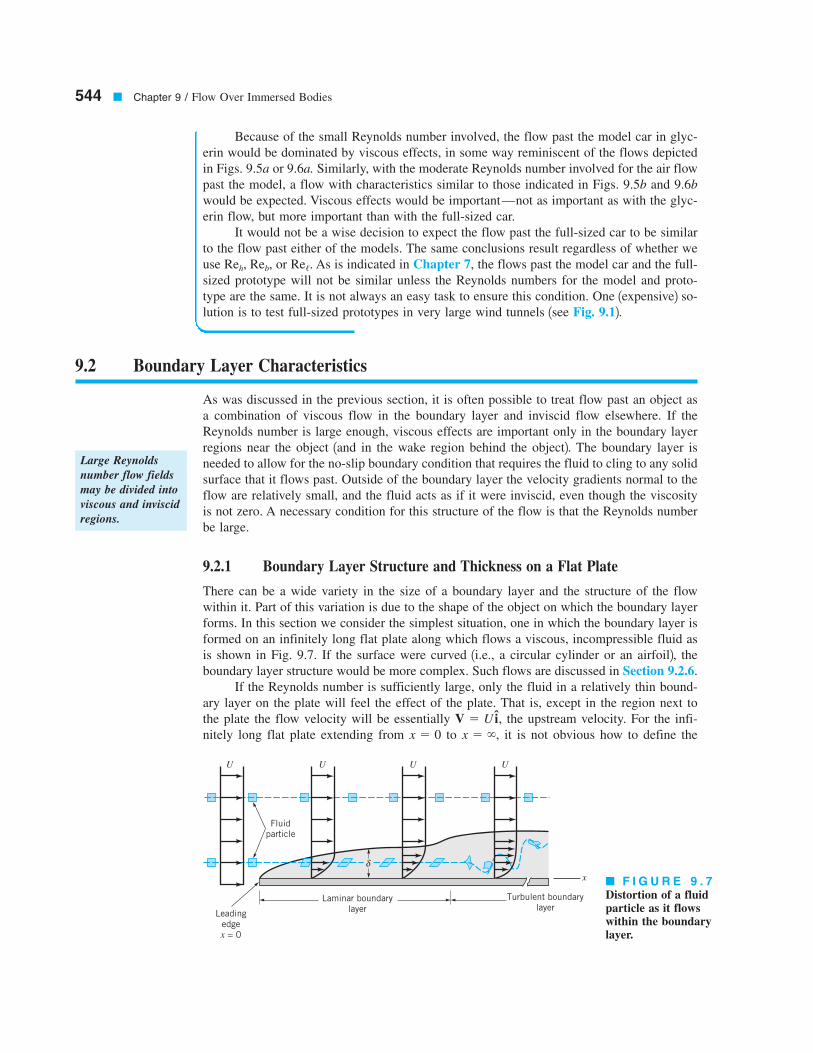
forms. In this section we consider the simplest situation, one in which the boundary layer is
formed on an infinitely long flat plate along which flows a viscous, incompressible fluid as
is shown in Fig. 9.7. If the surface were curved 1i.e., a circular cylinder or an airfoil2, the
boundary layer structure would be more complex. Such flows are discussed in Section 9.2.6.
If the Reynolds number is sufficiently large, only the fluid in a relatively thin bound-
ary layer on the plate will feel the effect of the plate. That is, except in the region next to
the plate the flow velocity will be essentially the upstream velocity. For the infi-
nitely long flat plate extending from to it is not obvious how to define thex 5 `,x 5 0
V 5 U i,
Large Reynolds
number flow fields
may be divided into
viscous and inviscid
regions.
■ F I G U R E 9 . 7
Distortion of a fluidparticle as it flowswithin the boundarylayer.
δ
U U U U
Fluid
particle
Leading
edge
x = 0
Laminar boundary
layer
Turbulent boundary
layer
x
Reynolds number because there is no characteristic length. The plate has no thickness and
is not of finite length!
For a finite length plate, it is clear that the plate length, can be used as the charac-
teristic length. For an infinitely long plate we use x, the coordinate distance along the plate
from the leading edge, as the characteristic length and define the Reynolds number as
Thus, for any fluid or upstream velocity the Reynolds number will be suffi-
ciently large for boundary layer type flow 1i.e., Fig. 9.5c2 if the plate is long enough. Phys-
ically, this means that the flow situations illustrated in Fig. 9.5 could be thought of as occurring
on the same plate, but should be viewed by looking at longer portions of the plate as we step
away from the plate to see the flows in Fig. 9.5a, 9.5b, and 9.5c, respectively.
If the plate is sufficiently long, the Reynolds number is sufficiently large
so that the flow takes on its boundary layer character 1except very near the leading edge2.The details of the flow field near the leading edge are lost to our eyes because we are stand-
ing so far from the plate that we cannot make out these details. On this scale 1Fig. 9.5c2 the
plate has negligible effect on the fluid ahead of the plate. The presence of the plate is felt
only in the relatively thin boundary layer and wake regions. As previously noted, Prandtl in
1904 was the first to hypothesize such a concept. It has become one of the major turning
points in fluid mechanics analysis.
A better appreciation of the structure of the boundary layer flow can be obtained by
considering what happens to a fluid particle that flows into the boundary layer. As is indi-
cated in Fig. 9.7, a small rectangular particle retains its original shape as it flows in the uni-
form flow outside of the boundary layer. Once it enters the boundary layer, the particle be-
gins to distort because of the velocity gradient within the boundary layer—the top of the
particle has a larger speed than its bottom. The fluid particles do not rotate as they flow along
outside the boundary layer, but they begin to rotate once they pass through the fictitious
boundary layer surface and enter the world of viscous flow. The flow is said to be irrota-
tional outside the boundary layer and rotational within the boundary layer. 1In terms of the
kinematics of fluid particles as is discussed in Section 6.1, the flow outside the boundary
layer has zero vorticity, and the flow within the boundary layer has nonzero vorticity.2At some distance downstream from the leading edge, the boundary layer flow becomes
turbulent and the fluid particles become greatly distorted because of the random, irregular
nature of the turbulence. One of the distinguishing features of turbulent flow is the occur-
rence of irregular mixing of fluid parcels that range in size from the smallest fluid particles
up to those comparable in size with the object of interest. For laminar flow, mixing occurs
only on the molecular scale. This molecular scale is orders of magnitude smaller in size than
typical size scales for turbulent flow mixing. The transition from laminar to turbulent flow
occurs at a critical value of the Reynolds number, on the order of to
depending on the roughness of the surface and the amount of turbulence in the upstream
flow, as is discussed in Section 9.2.4.
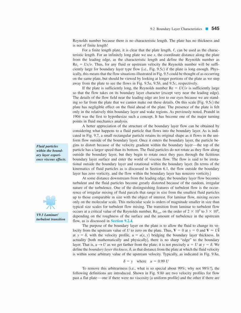
The purpose of the boundary layer on the plate is to allow the fluid to change its ve-
locity from the upstream value of U to zero on the plate. Thus, at and
at with the velocity profile, bridging the boundary layer thickness. In
actuality 1both mathematically and physically2, there is no sharp “edge” to the boundary
layer. That is, as we get farther from the plate; it is not precisely at We
define the boundary layer thickness, as that distance from the plate at which the fluid velocity
is within some arbitrary value of the upstream velocity. Typically, as indicated in Fig. 9.8a,
To remove this arbitrariness 1i.e., what is so special about 99%; why not 98%?2, the
following definitions are introduced. Shown in Fig. 9.8b are two velocity profiles for flow
past a flat plate—one if there were no viscosity 1a uniform profile2 and the other if there are
d 5 y where u 5 0.99 U
d,
y 5 d.u 5 UuSU
u 5 u1x, y2y 5 d,
V < U iy 5 0V 5 0
3 3 106,2 3 105Rexcr,
Re 5 U//n
Rex 5 Ux/n.
/,
9.2 Boundary Layer Characteristics ■ 545
Fluid particles
within the bound-
ary layer experi-
ence viscous effects.
V9.3 Laminar/
turbulent transition
viscosity and zero slip at the wall 1the boundary layer profile2. Because of the velocity deficit,
within the boundary layer, the flowrate across section b–b is less than that across
section a–a. However, if we displace the plate at section a–a by an appropriate amount
the boundary layer displacement thickness, the flowrates across each section will be identi-
cal. This is true if
where b is the plate width. Thus,
(9.3)
The displacement thickness represents the amount that the thickness of the body must
be increased so that the fictitious uniform inviscid flow has the same mass flowrate proper-
ties as the actual viscous flow. It represents the outward displacement of the streamlines
caused by the viscous effects on the plate. This idea allows us to simulate the presence that
the boundary layer has on the flow outside of the boundary layer by adding the displacement
thickness to the actual wall and treating the flow over the thickened body as an inviscid flow.
The displacement thickness concept is illustrated in Example 9.3.
d* 5 #`
0
a1 2u
Ub dy
d*b U 5 #`
0
1U 2 u2b dy
d*,
U 2 u,
546 ■ Chapter 9 / Flow Over Immersed Bodies
The boundary layer
displacement thick-
ness is defined in
terms of volumetric
flowrate.
U U U
δ*
δ
a b
Equal
areas
y a bu = 0.99 U = 0
u = Uµ
≠ 0u = u(y)
µ
U – u
(a) (b)
EXAMPLE
9.3
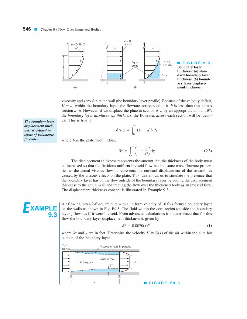
Air flowing into a 2-ft-square duct with a uniform velocity of 10 ftys forms a boundary layer
on the walls as shown in Fig. E9.3. The fluid within the core region 1outside the boundary
layers2 flows as if it were inviscid. From advanced calculations it is determined that for this
flow the boundary layer displacement thickness is given by
(1)
where and x are in feet. Determine the velocity of the air within the duct but
outside of the boundary layer.
U 5 U1x2d*
d* 5 0.00701x21/2
■ F I G U R E 9 . 8
Boundary layerthickness: (a) stan-dard boundary layerthickness, (b) bound-ary layer displace-ment thickness.
(1) (2)
Inviscid core
2-ft square U(x)
x
δ∗
Viscous effects importantU1 =
10 ft/s
■ F I G U R E E 9 . 3
9.2 Boundary Layer Characteristics ■ 547
SOLUTION
If we assume incompressible flow 1a reasonable assumption because of the low velocities in-
volved2, it follows that the volume flowrate across any section of the duct is equal to that at
the entrance 1i.e., 2. That is,
According to the definition of the displacement thickness, the flowrate across section 122is the same as that for a uniform flow with velocity U through a duct whose walls have been
moved inward by That is,
(2)
By combining Eqs. 1 and 2 we obtain
or
(Ans)
Note that U increases in the downstream direction. For example, at
The viscous effects that cause the fluid to stick to the walls of the duct reduce
the effective size of the duct, thereby 1from conservation of mass principles2 causing the fluid
to accelerate. The pressure drop necessary to do this can be obtained by using the Bernoulli
equation 1Eq. 3.72 along the inviscid streamlines from section 112 to 122. 1Recall that this equa-
tion is not valid for viscous flows within the boundary layer. It is, however, valid for the in-
viscid flow outside the boundary layer.2 Thus,
Hence, with and we obtain
or
For example, at
If it were desired to maintain a constant velocity along the centerline of this entrance
region of the duct, the walls could be displaced outward by an amount equal to the bound-
ary layer displacement thickness, d*.
x 5 100 ft.p 5 20.0401 lb/ft2
p 5 0.119 c1 21
11 2 0.0070x1/224 d lb/ft2
51
2 12.38 3 1023 slugs/ft
32 c 110 ft/s22 2102
11 2 0.0079x1/224 ft2/s
2 d
p 51
2 r 1U 2
1 2 U 22p1 5 0r 5 2.38 3 1023 slugs/ft
3
p1 112rU
21 5 p 1
12rU
2
x 5 100 ft.
U 5 11.6 ft/s
U 510
11 2 0.0070x1/222 ft/s
40 ft3/s 5 4U11 2 0.0070x1/222
40 ft3/s 5 #122 u dA 5 U12 ft 2 2d*22
d*.
d*,
U1A1 5 10 ft/s 12 ft22 5 40 ft3/s 5 #122u dA
Q1 5 Q2
Another boundary layer thickness definition, the boundary layer momentum thickness,
is often used when determining the drag on an object. Again because of the velocity
deficit, in the boundary layer, the momentum flux across section b–b in Fig. 9.8 is
less than that across section a–a. This deficit in momentum flux for the actual boundary
layer flow is given by
which by definition is the momentum flux in a layer of uniform speed U and thickness
That is,
or
(9.4)
All three boundary layer thickness definitions, and are of use in boundary layer
analyses.
The boundary layer concept is based on the fact that the boundary layer is thin. For
the flat plate flow this means that at any location x along the plate, Similarly,
and Again, this is true if we do not get too close to the leading edge of the plate 1i.e.,
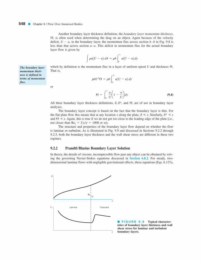
not closer than or so2.The structure and properties of the boundary layer flow depend on whether the flow
is laminar or turbulent. As is illustrated in Fig. 9.9 and discussed in Sections 9.2.2 through
9.2.5, both the boundary layer thickness and the wall shear stress are different in these two
regimes.
9.2.2 Prandtl /Blasius Boundary Layer Solution
In theory, the details of viscous, incompressible flow past any object can be obtained by solv-
ing the governing Navier-Stokes equations discussed in Section 6.8.2. For steady, two-
dimensional laminar flows with negligible gravitational effects, these equations 1Eqs. 6.127a,
Rex 5 Ux/n 5 1000
™ ! x.
d* ! xd ! x.
™,d, d*,
™ 5 #`
0
u
U a1 2
u
Ub dy
rbU 2™ 5 rb#
`
0
u1U 2 u2 dy
™.
# ru1U 2 u2 dA 5 rb#`
0
u1U 2 u2 dy
U 2 u,
™,
548 ■ Chapter 9 / Flow Over Immersed Bodies
The boundary layer
momentum thick-
ness is defined in
terms of momentum
flux.
τ
δ
w
x
x
x
Laminar Turbulent
Recr
■ F I G U R E 9 . 9 Typical character-istics of boundary layer thickness and wallshear stress for laminar and turbulentboundary layers.
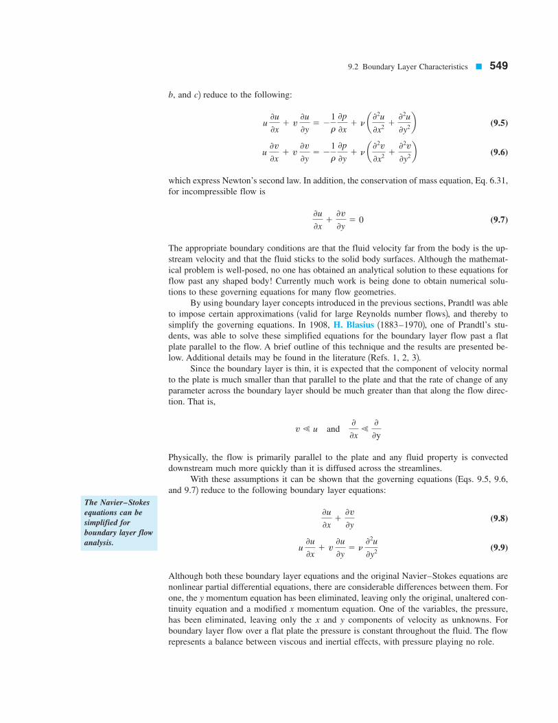
b, and c2 reduce to the following:
(9.5)
(9.6)
which express Newton’s second law. In addition, the conservation of mass equation, Eq. 6.31,
for incompressible flow is
(9.7)
The appropriate boundary conditions are that the fluid velocity far from the body is the up-
stream velocity and that the fluid sticks to the solid body surfaces. Although the mathemat-
ical problem is well-posed, no one has obtained an analytical solution to these equations for
flow past any shaped body! Currently much work is being done to obtain numerical solu-
tions to these governing equations for many flow geometries.
By using boundary layer concepts introduced in the previous sections, Prandtl was able
to impose certain approximations 1valid for large Reynolds number flows2, and thereby to
simplify the governing equations. In 1908, H. Blasius 11883–19702, one of Prandtl’s stu-
dents, was able to solve these simplified equations for the boundary layer flow past a flat
plate parallel to the flow. A brief outline of this technique and the results are presented be-
low. Additional details may be found in the literature 1Refs. 1, 2, 32.Since the boundary layer is thin, it is expected that the component of velocity normal
to the plate is much smaller than that parallel to the plate and that the rate of change of any
parameter across the boundary layer should be much greater than that along the flow direc-
tion. That is,
Physically, the flow is primarily parallel to the plate and any fluid property is convected
downstream much more quickly than it is diffused across the streamlines.
With these assumptions it can be shown that the governing equations 1Eqs. 9.5, 9.6,
and 9.72 reduce to the following boundary layer equations:
(9.8)
(9.9)
Although both these boundary layer equations and the original Navier–Stokes equations are
nonlinear partial differential equations, there are considerable differences between them. For
one, the y momentum equation has been eliminated, leaving only the original, unaltered con-
tinuity equation and a modified x momentum equation. One of the variables, the pressure,
has been eliminated, leaving only the x and y components of velocity as unknowns. For
boundary layer flow over a flat plate the pressure is constant throughout the fluid. The flow
represents a balance between viscous and inertial effects, with pressure playing no role.
u 0u
0x1 v
0u
0y5 n 0
2u
0y2
0u
0x10v
0y
v ! u and 0
0x!0
0y
0u
0x10v
0y5 0
u 0v
0x1 v
0v
0y5 2
1
r
0p
0y1 n a 02v
0x210
2v
0y2b
u 0u
0x1 v
0u
0y5 2
1
r
0p
0x1 n a 02u
0x210
2u
0y2b
9.2 Boundary Layer Characteristics ■ 549
The Navier–Stokes
equations can be
simplified for
boundary layer flow
analysis.
The boundary conditions for the governing boundary layer equations are that the fluid
sticks to the plate
(9.10)
and that outside of the boundary layer the flow is the uniform upstream flow That is,
(9.11)
Mathematically, the upstream velocity is approached asymptotically as one moves away from
the plate. Physically, the flow velocity is within 1% of the upstream velocity at a distance of
from the plate.
In mathematical terms, the Navier–Stokes equations 1Eqs. 9.5, 9.62 and the continuity
equation 1Eq. 9.72 are elliptic equations, whereas the equations for boundary layer flow1Eqs. 9.8 and 9.92 are parabolic equations. The nature of the solutions to these two sets of
equations, therefore, is different. Physically, this fact translates to the idea that what happens
downstream of a given location in a boundary layer cannot affect what happens upstream of
that point. That is, whether the plate shown in Fig. 9.5c ends with length or is extended to
length the flow within the first segment of length will be the same. In addition, the
presence of the plate has no effect on the flow ahead of the plate.
In general, the solutions of nonlinear partial differential equations 1such as the bound-
ary layer equations, Eqs. 9.8 and 9.92 are extremely difficult to obtain. However, by apply-
ing a clever coordinate transformation and change of variables, Blasius reduced the partial
differential equations to an ordinary differential equation that he was able to solve. A brief
description of this process is given below. Additional details can be found in standard books
dealing with boundary layer flow 1Refs. 1, 22.It can be argued that in dimensionless form the boundary layer velocity profiles on a
flat plate should be similar regardless of the location along the plate. That is,
where is an unknown function to be determined. In addition, by applying an order of
magnitude analysis of the forces acting on fluid within the boundary layer, it can be shown
that the boundary layer thickness grows as the square root of x and inversely proportional to
the square root of U. That is,
Such a conclusion results from a balance between viscous and inertial forces within the
boundary layer and from the fact that the velocity varies much more rapidly in the direction
across the boundary layer than along it.
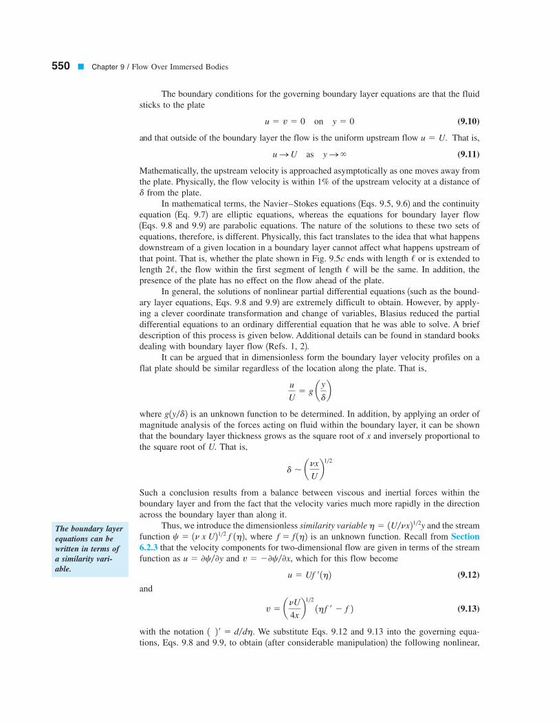
Thus, we introduce the dimensionless similarity variable and the stream
function where is an unknown function. Recall from Section
6.2.3 that the velocity components for two-dimensional flow are given in terms of the stream
function as and which for this flow become
(9.12)
and
(9.13)
with the notation We substitute Eqs. 9.12 and 9.13 into the governing equa-
tions, Eqs. 9.8 and 9.9, to obtain 1after considerable manipulation2 the following nonlinear,
1 2 ¿ 5 d/dh.
v 5 anU4xb1/2
1h f ¿ 2 f 2
u 5 Uf ¿ 1h2v 5 20c/0x,u 5 0c/0y
f 5 f 1h2c 5 1n x U21/2 f 1h2, h 5 1U/nx21/2y
d , anxUb1/2
g1y/d2
u
U5 g ay
db
/2/,
/
d
uSU as yS`
u 5 U.
u 5 v 5 0 on y 5 0
550 ■ Chapter 9 / Flow Over Immersed Bodies
The boundary layer
equations can be
written in terms of
a similarity vari-
able.

third-order ordinary differential equation:
(9.14a)
The boundary conditions given in Eqs. 9.10 and 9.11 can be written as
(9.14b)
The original partial differential equation and boundary conditions have been reduced to an
ordinary differential equation by use of the similarity variable The two independent vari-
ables, x and y, were combined into the similarity variable in a fashion that reduced the par-
tial differential equation 1and boundary conditions2 to an ordinary differential equation. This
type of reduction is not generally possible. For example, this method does not work on the
full Navier-Stokes equations, although it does on the boundary layer equations 1Eqs. 9.8
and 9.92.Although there is no known analytical solution to Eq. 9.14, it is relatively easy to
integrate this equation on a computer. The dimensionless boundary layer profile,
obtained by numerical solution of Eq. 9.14 1termed the Blasius solution2, is sketched in
Fig. 9.10a and is tabulated in Table 9.1. The velocity profiles at different x locations are sim-
ilar in that there is only one curve necessary to describe the velocity at any point in the bound-
ary layer. Because the similarity variable contains both x and y, it is seen from Fig. 9.10b
that the actual velocity profiles are a function of both x and y. The profile at location is
the same as that at except that the y coordinate is stretched by a factor of
From the solution it is found that when Thus,
(9.15)
or
where It can also be shown that the displacement and momentum thicknesses
are given by
(9.16)
and
(9.17)
As postulated, the boundary layer is thin provided that is large as
With the velocity profile known, it is an easy matter to determine the wall shear stress,
where the velocity gradient is evaluated at the plate. The value of
at can be obtained from the Blasius solution to give
(9.18)
Note that the shear stress decreases with increasing x because of the increasing thickness of
the boundary layer—the velocity gradient at the wall decreases with increasing x. Also,
varies as not as U as it does for fully developed laminar pipe flow. These variations are
discussed in Section 9.2.3.
U3/2,
tw
tw 5 0.332U3/2 Brm
x
y 5 0
0u/0ytw 5 m 10u/0y2y50,
RexS`2.1i.e., d/xS 0Rex
™
x5
0.664
1Rex
d*
x5
1.721
1Rex
Rex 5 Ux/n.
d
x5
5
1Rex
d 5 5 Anx
U
h 5 5.0.u/U < 0.99
1x2 /x121/2.x2
x1
h
u/U 5 f ¿ 1h2,
h.
f 5 f ¿ 5 0 at h 5 0 and f ¿ S 1 as hS`
2f ‡ 1 f f – 5 0
9.2 Boundary Layer Characteristics ■ 551
Laminar, flat plate
boundary layer
thickness grows as
the square root of
the distance from
the leading edge.

9.2.3 Momentum-Integral Boundary Layer Equation
for a Flat Plate
One of the important aspects of boundary layer theory is the determination of the drag
caused by shear forces on a body. As was discussed in the previous section, such results
can be obtained from the governing differential equations for laminar boundary layer flow.
Since these solutions are extremely difficult to obtain, it is of interest to have an alternative
approximate method. The momentum integral method described in this section provides
such an alternative.
We consider the uniform flow past a flat plate and the fixed control volume as shown
in Fig. 9.11. In agreement with advanced theory and experiment, we assume that the pres-
sure is constant throughout the flow field. The flow entering the control volume at the lead-
ing edge of the plate [section 112] is uniform, while the velocity of the flow exiting the con-
trol volume [section 122] varies from the upstream velocity at the edge of the boundary layer
to zero velocity on the plate.
The fluid adjacent to the plate makes up the lower portion of the control surface. The
upper surface coincides with the streamline just outside the edge of the boundary layer at
section 122. It need not 1in fact, does not2 coincide with the edge of the boundary layer ex-
cept at section 122. If we apply the x component of the momentum equation 1Eq. 5.222 to the
steady flow of fluid within this control volume we obtain
a Fx 5 r#112
uV ? n dA 1 r #122
uV ? n dA
552 ■ Chapter 9 / Flow Over Immersed Bodies
■ F I G U R E 9 . 1 0 Blasius boundary layer profile: (a) boundary layer profile in dimen-sionless form using the similarity variable (b) similar boundary layer profiles at differentlocations along the flat plate.
H,
x 4 = 16 x1
x 3 = 9 x1
x 2 = 4 x1
x = x1
x 5 = 25 x1
δ ∼ x
u
U
(b)
(a)
0
δ1
δ1δ2 = 2
δ1δ3 = 3
y
1.00.80.60.40.200 0
1
2
3
4
5
u__U
u__U
η≈ 0.99 at ≈ 5
f ′ ( ) =η
= y
( )
U __ vx
1/ 2
η
The momentum in-
tegral method pro-
vides an approxi-
mate technique to
analyze boundary
layer flow.
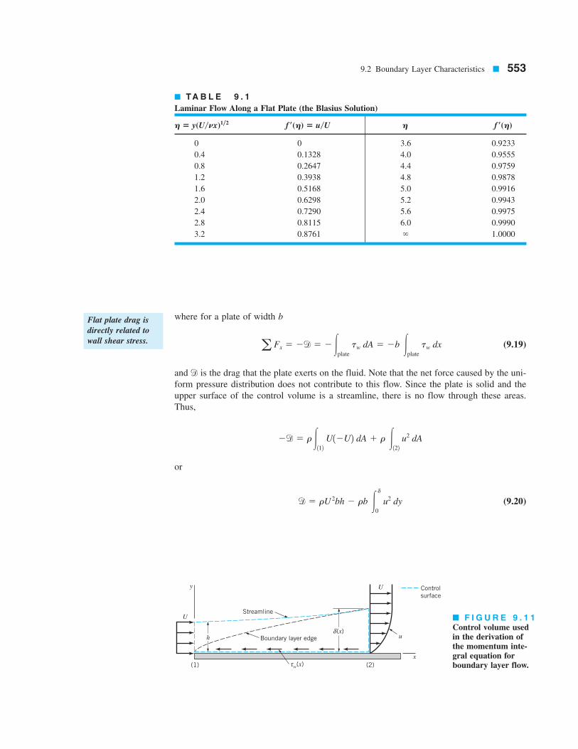
where for a plate of width b
(9.19)
and is the drag that the plate exerts on the fluid. Note that the net force caused by the uni-
form pressure distribution does not contribute to this flow. Since the plate is solid and the
upper surface of the control volume is a streamline, there is no flow through these areas.
Thus,
or
(9.20)d 5 rU 2bh 2 rb #d
0
u2 dy
2d 5 r#112
U12U2 dA 1 r #122
u2 dA
d
a Fx 5 2d 5 2#plate
tw dA 5 2b #plate
tw dx
9.2 Boundary Layer Characteristics ■ 553
■ TA B L E 9 . 1
Laminar Flow Along a Flat Plate (the Blasius Solution)
( ) ( ) ( )
0 0 3.6 0.9233
0.4 0.1328 4.0 0.9555
0.8 0.2647 4.4 0.9759
1.2 0.3938 4.8 0.9878
1.6 0.5168 5.0 0.9916
2.0 0.6298 5.2 0.9943
2.4 0.7290 5.6 0.9975
2.8 0.8115 6.0 0.9990
3.2 0.8761 1.0000`
Hf 9H5 u/UHf 91y2U/NxH 5 y
Flat plate drag is
directly related to
wall shear stress.
Streamline
Boundary layer edge
Control
surface
x
u
U
(2)(1)
U
y
hδ(x)
τw(x)
■ F I G U R E 9 . 1 1
Control volume usedin the derivation ofthe momentum inte-gral equation forboundary layer flow.

Although the height h is not known, it is known that for conservation of mass the
flowrate through section 112 must equal that through section 122, or
which can be written as
(9.21)
Thus, by combining Eqs. 9.20 and 9.21 we obtain the drag in terms of the deficit of mo-
mentum flux across the outlet of the control volume as
(9.22)
If the flow were inviscid, the drag would be zero, since we would have and the
right-hand side of Eq. 9.22 would be zero. 1This is consistent with the fact that if
.2 Equation 9.22 points out the important fact that boundary layer flow on a flat plate
is governed by a balance between shear drag 1the left-hand side of Eq. 9.222 and a decrease
in the momentum of the fluid 1the right-hand side of Eq. 9.222. As x increases, increases
and the drag increases. The thickening of the boundary layer is necessary to overcome the
drag of the viscous shear stress on the plate. This is contrary to horizontal fully developed
pipe flow in which the momentum of the fluid remains constant and the shear force is over-
come by the pressure gradient along the pipe.
The development of Eq. 9.22 and its use was first put forth in 1921 by T. von
Karman 11881–19632, a Hungarian/German aerodynamicist. By comparing Eqs. 9.22 and
9.4 we see that the drag can be written in terms of the momentum thickness, as
(9.23)
Note that this equation is valid for laminar or turbulent flows.
The shear stress distribution can be obtained from Eq. 9.23 by differentiating both sides
with respect to x to obtain
(9.24)
The increase in drag per length of the plate, occurs at the expense of an increase of
the momentum boundary layer thickness, which represents a decrease in the momentum of
the fluid.
Since 1see Eq. 9.192 it follows that
(9.25)dd
dx5 btw
d d 5 tw b dx
dd/dx,
dd
dx5 rbU 2
d™
dx
d 5 rbU 2 ™
™,
d
m 5 0
tw 5 0
u K U
d 5 rb#d
0
u1U 2 u2 dy
rU 2bh 5 rb#d
0
Uu dy
Uh 5 #d
0
u dy
554 ■ Chapter 9 / Flow Over Immersed Bodies
Drag on a flat plate
is related to mo-
mentum deficit
within the bound-
ary layer.

Hence, by combining Eqs. 9.24 and 9.25 we obtain the momentum integral equation for the
boundary layer flow on a flat plate
(9.26)
The usefulness of this relationship lies in the ability to obtain approximate boundary
layer results easily by using rather crude assumptions. For example, if we knew the detailed
velocity profile in the boundary layer 1i.e., the Blasius solution discussed in the previous sec-
tion2, we could evaluate either the right-hand side of Eq. 9.23 to obtain the drag, or the right-
hand side of Eq. 9.26 to obtain the shear stress. Fortunately, even a rather crude guess at the
velocity profile will allow us to obtain reasonable drag and shear stress results from Eq. 9.26.
This method is illustrated in Example 9.4.
tw 5 rU 2 d™
dx
9.2 Boundary Layer Characteristics ■ 555
EXAMPLE
9.4
Consider the laminar flow of an incompressible fluid past a flat plate at The bound-
ary layer velocity profile is approximated as for and for
as is shown in Fig. E9.4. Determine the shear stress by using the momentum integral equa-
tion. Compare these results with the Blasius results given by Eq. 9.18.
y 7 d,u 5 U0 # y # du 5 Uy/d
y 5 0.
Shear stress on a
flat plate is propor-
tional to the rate of
boundary layer
growth.
y
U u0
u = Uy/δ
δ
u = U
■ F I G U R E E 9 . 4
SOLUTION
From Eq. 9.26 the shear stress is given by
(1)
while for laminar flow we know that For the assumed profile we have
(2)
and from Eq. 9.4
™ 5 #`
0
u
U a1 2
u
Ub dy 5 #
d
0
u
U a1 2
u
Ub dy 5 #
d
0
ay
db a1 2
y
db dy
tw 5 m
U
d
tw 5 m10u/0y2y50.
tw 5 rU 2 d™
dx

As is illustrated in Example 9.4, the momentum integral equation, Eq. 9.26, can be
used along with an assumed velocity profile to obtain reasonable, approximate boundary layer
results. The accuracy of these results depends on how closely the shape of the assumed ve-
locity profile approximates the actual profile.
Thus, we consider a general velocity profile
and
where the dimensionless coordinate varies from 0 to 1 across the boundary layer.
The dimensionless function can be any shape we choose, although it should be a rea-
sonable approximation to the boundary layer profile. In particular, it should certainly satisfy
the boundary conditions at and at That is,
g102 5 0 and g112 5 1
y 5 d.u 5 Uy 5 0u 5 0
g1Y 2Y 5 y/d
u
U5 1 for Y 7 1
u
U5 g1Y 2 for 0 # Y # 1
556 ■ Chapter 9 / Flow Over Immersed Bodies
or
(3)
Note that as yet we do not know the value of 1but suspect that it should be a function of x2. By combining Eqs. 1, 2, and 3 we obtain the following differential equation for
or
This can be integrated from the leading edge of the plate, 1where 2 to an arbi-
trary location x where the boundary layer thickness is The result is
or
(4)
Note that this approximate result 1i.e., the velocity profile is not actually the simple straight
line we assumed2 compares favorably with the 1much more laborious to obtain2 Blasius re-
sult given by Eq. 9.15.
The wall shear stress can also be obtained by combining Eqs. 1, 3, and 4 to give
(Ans)
Again this approximate result is close 1within 13%2 to the Blasius value of given by
Eq. 9.18.
tw
tw 5 0.289U3/2 Brm
x
d 5 3.46 Bnx
U
d2
25
6m
rU x
d.
d 5 0x 5 0
d dd 56m
rU dx
mU
d5rU 2
6
dd
dx
d:
d
™ 5d
6
Approximate veloc-
ity profiles are used
in the momentum
integral equation.
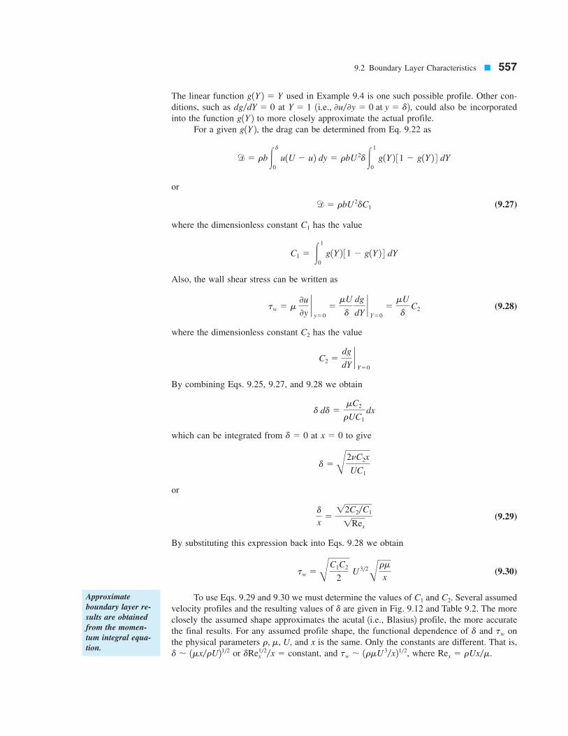
The linear function used in Example 9.4 is one such possible profile. Other con-
ditions, such as at could also be incorporated
into the function to more closely approximate the actual profile.
For a given the drag can be determined from Eq. 9.22 as
or
(9.27)
where the dimensionless constant has the value
Also, the wall shear stress can be written as
(9.28)
where the dimensionless constant has the value
By combining Eqs. 9.25, 9.27, and 9.28 we obtain
which can be integrated from at to give
or
(9.29)
By substituting this expression back into Eqs. 9.28 we obtain
(9.30)
To use Eqs. 9.29 and 9.30 we must determine the values of and Several assumed
velocity profiles and the resulting values of are given in Fig. 9.12 and Table 9.2. The more
closely the assumed shape approximates the acutal 1i.e., Blasius2 profile, the more accurate
the final results. For any assumed profile shape, the functional dependence of and on
the physical parameters and x is the same. Only the constants are different. That is,
or and where Rex 5 rUx/m.tw , 1rmU 3/x21/2,dRe1/2
x /x 5 constant,d , 1mx/rU21/2
r, m, U,
twd
d
C2.C1
tw 5 BC1C2
2 U 3/2 A
rm
x
d
x512C2/C1
1Rex
d 5 B2nC2x
UC1
x 5 0d 5 0
d dd 5mC2
rUC1
dx
C2 5dg
dY`Y50
C2
tw 5 m 0u
0y`y50
5mU
d
dg
dY`Y50
5mU
d C2
C1 5 #1
0
g1Y 2 31 2 g1Y 2 4 dY
C1
d 5 rbU 2dC1
d 5 rb#d
0
u1U 2 u2 dy 5 rbU 2d#1
0
g1Y 2 31 2 g1Y 2 4 dY
g1Y 2,g1Y 2 1i.e., 0u/0y 5 0 at y 5 d2,Y 5 1dg/dY 5 0
g1Y 2 5 Y
9.2 Boundary Layer Characteristics ■ 557
Approximate
boundary layer re-
sults are obtained
from the momen-
tum integral equa-
tion.

It is often convenient to use the dimensionless local friction coefficient, defined as
(9.31)
to express the wall shear stress. From Eq. 9.30 we obtain the approximate value
while the Blasius solution result is given by
(9.32)
These results are also indicated in Table 9.2.
cf 50.664
1Rex
cf 5 12C1C2 Am
rUx512C1C2
1Rex
cf 5tw
12 rU
2
cf ,
558 ■ Chapter 9 / Flow Over Immersed Bodies
The local friction
coefficient is the di-
mensionless wall
shear stress.
Parabolic
Blasius
Sine wave
Cubic
Linear
1.00.500
0.5
1.0
y__δ
u__U
■ F I G U R E 9 . 1 2 Typical approximate boundary layer profilesused in the momentum integralequation.
■ TA B L E 9 . 2
Flat Plate Momentum-Integral Results for Various Assumed Laminar Flow Velocity Profiles
Profile Character
a. Blasius solution 5.00 0.664 1.328
b. Linear 3.46 0.578 1.156
c. Parabolic 5.48 0.730 1.460
d. Cubic 4.64 0.646 1.292
e. Sine wave 4.79 0.655 1.310u/U 5 sin 3p1 y/d2/2 4
u/U 5 31 y/d2/2 2 1y/d23/2
u/U 5 2y/d 2 1y/d22
u/U 5 y/d
CDfRe<
1/2cfRex1/2DRex
1/2/x

For a flat plate of length and width b, the net friction drag, can be expressed in
terms of the friction drag coefficient, as
or
(9.33)
We use the above approximate value of to obtain
where is the Reynolds number based on the plate length. The corresponding
value obtained from the Blasius solution 1Eq. 9.322 gives
These results are also indicated in Table 9.2.
The momentum-integral boundary layer method provides a relatively simple technique
to obtain useful boundary layer results. As is discussed in Sections 9.2.5 and 9.2.6, this tech-
nique can be extended to boundary layer flows on curved surfaces 1where the pressure and
fluid velocity at the edge of the boundary layer are not constant2 and to turbulent flows.
9.2.4 Transition from Laminar to Turbulent Flow
The analytical results given in Table 9.2 are restricted to laminar boundary layer flows along
a flat plate with zero pressure gradient. They agree quite well with experimental results up
to the point where the boundary layer flow becomes turbulent, which will occur for any free
stream velocity and any fluid provided the plate is long enough. This is true because the pa-
rameter that governs the transition to turbulent flow is the Reynolds number—in this case
the Reynolds number based on the distance from the leading edge of the plate,
The value of the Reynolds number at the transition location is a rather complex func-
tion of various parameters involved, including the roughness of the surface, the curvature of
the surface 1e.g., a flat plate or a sphere2, and some measure of the disturbances in the flow
outside the boundary layer. On a flat plate with a sharp leading edge in a typical air stream,
the transition takes place at a distance x from the leading edge given by to
Unless otherwise stated, we will use in our calculations.
The actual transition from laminar to turbulent boundary layer flow may occur over a
region of the plate, not at a specific single location. This occurs, in part, because of the spot-
tiness of the transition. Typically, the transition begins at random locations on the plate in
the vicinity of These spots grow rapidly as they are convected downstream un-
til the entire width of the plate is covered with turbulent flow. The photo shown in Fig. 9.13
illustrates this transition process.
The complex process of transition from laminar to turbulent flow involves the insta-
bility of the flow field. Small disturbances imposed on the boundary layer flow 1i.e., from a
vibration of the plate, a roughness of the surface, or a “wiggle” in the flow past the plate2will either grow 1instability2 or decay 1stability2, depending on where the disturbance is in-
troduced into the flow. If these disturbances occur at a location with they willRex 6 Rexcr
Rex 5 Rexcr.
Rexcr 5 5 3 1053 3 106.
Rexcr 5 2 3 105
Rex 5 Ux/n.
CDf 51.328
1Re/
Re/ 5 U//n
CDf 518C1C2
1Re/
cf 5 12C1C2m/rUx21/2
CDf 51
/ #/
0
cf dx
CDf 5
df
12 rU
2b/5
b #/
0
tw dx
12 rU
2b/
CDf,
df,/
9.2 Boundary Layer Characteristics ■ 559
The friction drag
coefficient is an in-
tegral of the local
friction coefficient.

die out, and the boundary layer will return to laminar flow at that location. Disturbances im-
posed at a location with will grow and transform the boundary layer flow down-
stream of this location into turbulence. The study of the initiation, growth, and structure of
these turbulent bursts or spots is an active area of fluid mechanics research.
Transition from laminar to turbulent flow also involves a noticeable change in the shape
of the boundary layer velocity profile. Typical profiles obtained in the neighborhood of the
transition location are indicated in Fig. 9.14. The turbulent profiles are flatter, have a larger
velocity gradient at the wall, and produce a larger boundary layer thickness than do the lam-
inar profiles.
Rex 7 Rexcr
560 ■ Chapter 9 / Flow Over Immersed Bodies
The boundary layer
on a flat plate will
become turbulent if
the plate is long
enough.
■ F I G U R E 9 . 1 4 Typicalboundary layer profiles on a flat platefor laminar, transitional, and turbulentflow (Ref. 1).
■ F I G U R E 9 . 1 3
Turbulent spots and the tran-sition from laminar to turbu-lent boundary layer flow on aflat plate. Flow from left toright. (Photograph courtesy of B. Cantwell, Stanford University.)
x = 5.25 ft
x = 6.76 ft
x = 8.00 ft
U = 89 ft/s; air flow
Transitional
Turbulent
Laminar
0.06
0.05
0.04
0.03
0.02
0.01
00 0.2 0.4 0.6 0.8 1
u__U
y, f
t
9.2.5 Turbulent Boundary Layer Flow
The structure of turbulent boundary layer flow is very complex, random, and irregular. It
shares many of the characteristics described for turbulent pipe flow in Section 8.3. In par-
ticular, the velocity at any given location in the flow is unsteady in a random fashion. The
flow can be thought of as a jumbled mix of interwined eddies 1or swirls2 of different sizes1diameters and angular velocities2. The various fluid quantities involved 1i.e., mass, momen-
tum, energy2 are convected downstream in the free-stream direction as in a laminar bound-
ary layer. For turbulent flow they are also convected across the boundary layer 1in the di-
rection perpendicular to the plate2 by the random transport of finite-sized fluid particles
associated with the turbulent eddies. There is considerable mixing involved with these finite-
9.2 Boundary Layer Characteristics ■ 561
Random transport
of finite-sized fluid
particles occurs
within turbulent
boundary layers.
EXAMPLE
9.5
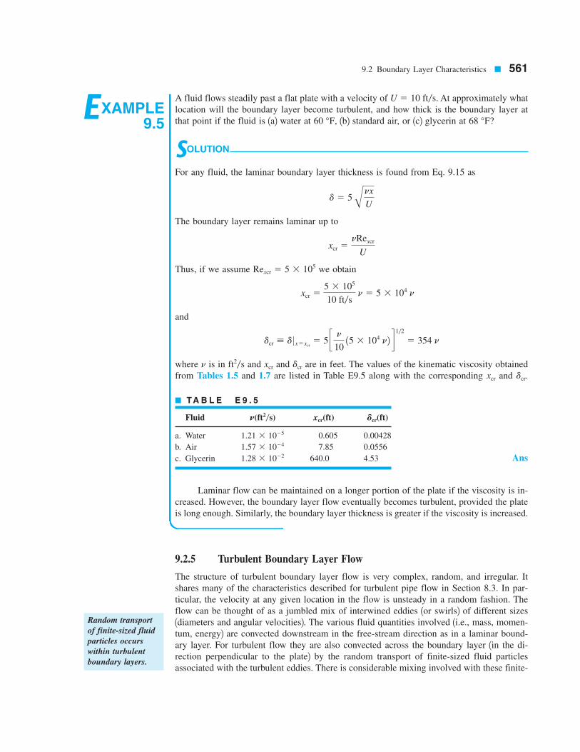
A fluid flows steadily past a flat plate with a velocity of At approximately what
location will the boundary layer become turbulent, and how thick is the boundary layer at
that point if the fluid is 1a2 water at 1b2 standard air, or 1c2 glycerin at
SOLUTION
For any fluid, the laminar boundary layer thickness is found from Eq. 9.15 as
The boundary layer remains laminar up to
Thus, if we assume we obtain
and
where is in and and are in feet. The values of the kinematic viscosity obtained
from Tables 1.5 and 1.7 are listed in Table E9.5 along with the corresponding and dcr.xcr
dcrxcrft2/sn
dcr ; d 0 x5xcr5 5 c n
10 15 3 104 n2 d 1/2
5 354 n
xcr 55 3 105
10 ft/s n 5 5 3 104 n
Rexcr 5 5 3 105
xcr 5nRexcr
U
d 5 5 Anx
U
68 °F?60 °F,
U 5 10 ft/s.
Laminar flow can be maintained on a longer portion of the plate if the viscosity is in-
creased. However, the boundary layer flow eventually becomes turbulent, provided the plate
is long enough. Similarly, the boundary layer thickness is greater if the viscosity is increased.
■ TA B L E E 9 . 5
Fluid ( ) (ft) (ft)
a. Water 0.605 0.00428
b. Air 7.85 0.0556
c. Glycerin 640.0 4.531.28 3 1022
1.57 3 1024
1.21 3 1025
Dcrxcrft2/sN
Ans

562 ■ Chapter 9 / Flow Over Immersed Bodies
EXAMPLE
9.6
Consider turbulent flow of an incompressible fluid past a flat plate. The boundary layer ve-
locity profile is assumed to be for and for
as shown in Fig. E9.6. This is a reasonable approximation of experimentally observed pro-
files, except very near the plate where this formula gives at Note the dif-
ferences between the assumed turbulent profile and the laminar profile. Also assume that the
shear stress agrees with the experimentally determined formula:
(1)
Determine the boundary layer thicknesses and and the wall shear stress, as a
function of x. Determine the friction drag coefficient,
SOLUTION
Whether the flow is laminar or turbulent, it is true that the drag force is accounted for by a
reduction in the momentum of the fluid flowing past the plate. The shear is obtained from
CDf.
tw,™d, d*,
tw 5 0.0225rU 2 a nUdb1/4
y 5 0.0u/0y 5 `
Y 7 1u 5 UY 5 y/d # 1u/U 5 1y/d21/ 75 Y1/ 7
There are no exact
solutions available
for turbulent
boundary layer
flows.
sized eddies—considerably more than is associated with the mixing found in laminar flow
where it is confined to the molecular scale. Although there is considerable random motion
of fluid particles perpendicular to the plate, there is very little net transfer of mass across the
boundary layer—the largest flowrate by far is parallel to the plate.
There is, however, a considerable net transfer of x component of momentum perpen-
dicular to the plate because of the random motion of the particles. Fluid particles moving
toward the plate 1in the negative y direction2 have some of their excess momentum 1they come
from areas of higher velocity2 removed by the plate. Conversely, particles moving away from
the plate 1in the positive y direction2 gain momentum from the fluid 1they come from areas of
lower velocity2. The net result is that the plate acts as a momentum sink, continually extracting
momentum from the fluid. For laminar flows, such cross-stream transfer of these properties
takes place solely on the molecular scale. For turbulent flow the randomness is associated with
fluid particle mixing. Consequently, the shear force for turbulent boundary layer flow is con-
siderably greater than it is for laminar boundary layer flow 1see Section 8.3.22.There are no “exact” solutions for turbulent boundary layer flow. As is discussed in
Section 9.2.2, it is possible to solve the Prandtl boundary layer equations for laminar flow
past a flat plate to obtain the Blasius solution 1which is “exact” within the framework of the
assumptions involved in the boundary layer equations2. Since there is no precise expression
for the shear stress in turbulent flow 1see Section 8.32, solutions are not available for turbu-
lent flow. However, considerable headway has been made in obtaining numerical 1computer2solutions for turbulent flow by using approximate shear stress relationships. Also, progress
is being made in the area of direct, full numerical integration of the basic governing equa-
tions, the Navier-Stokes equations.
Approximate turbulent boundary layer results can also be obtained by use of the mo-
mentum integral equation, Eq. 9.26, which is valid for either laminar or turbulent flow. What
is needed for the use of this equation are reasonable approximations to the velocity profile
where and u is the time-averaged velocity 1the overbar notation, of
Section 8.3.2 has been dropped for convenience2 and a functional relationship describing the
wall shear stress. For laminar flow the wall shear stress was used as In
theory, such a technique should work for turbulent boundary layers also. However, as is dis-
cussed in Section 8.3, the details of the velocity gradient at the wall are not well understood
for turbulent flow. Thus, it is necessary to use some empirical relationship for the wall shear
stress. This is illustrated in Example 9.6.
tw 5 m10u/0y2y50.
u,Y 5 y/du 5 U g1Y 2,

9.2 Boundary Layer Characteristics ■ 563
■ F I G U R E E 9 . 6
Laminar
u__U
u__U
=y__δ
y __
δ
Turbulent
1.00.500
0.2
0.4
0.6
0.8
1.0
Y =
( )1__
7
Eq. 9.26 in terms of the rate at which the momentum boundary layer thickness, increases
with distance along the plate as
For the assumed velocity profile, the boundary layer momentum thickness is obtained
from Eq. 9.4 as
or by integration
(2)
where is an unknown function of x. By combining the assumed shear force dependence1Eq. 12 with Eq. 2, we obtain the following differential equation for
or
This can be integrated from at to obtain
(3) (Ans)
or in dimensionless form
d
x5
0.370
Rex1/5
d 5 0.370 a nUb1/5
x4/5
x 5 0d 5 0
d1/4 dd 5 0.231 a nUb1/4
dx
0.0225rU 2 a nUdb1/4
57
72 rU 2
dd
dx
d:
d
™ 5 d#1
0 Y
1/ 7 11 2 Y1/ 72 dY 57
72 d
™ 5 #`
0
u
U a1 2
u
Ub dy 5 d#
1
0
u
U a1 2
u
Ub dY
tw 5 rU 2 d™
dx
™,
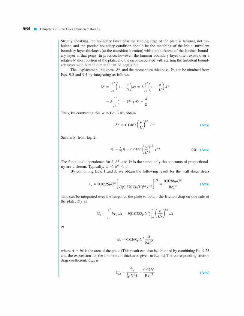
564 ■ Chapter 9 / Flow Over Immersed Bodies
Strictly speaking, the boundary layer near the leading edge of the plate is laminar, not tur-
bulent, and the precise boundary condition should be the matching of the initial turbulent
boundary layer thickness 1at the transition location2 with the thickness of the laminar bound-
ary layer at that point. In practice, however, the laminar boundary layer often exists over a
relatively short portion of the plate, and the error associated with starting the turbulent bound-
ary layer with at can be negligible.
The displacement thickness, and the momentum thickness, can be obtained from
Eqs. 9.3 and 9.4 by integrating as follows:
Thus, by combining this with Eq. 3 we obtain
(Ans)
Similarly, from Eq. 2,
(4) (Ans)
The functional dependence for and is the same; only the constants of proportional-
ity are different. Typically,
By combining Eqs. 1 and 3, we obtain the following result for the wall shear stress
(Ans)
This can be integrated over the length of the plate to obtain the friction drag on one side of
the plate, as
or
where is the area of the plate. 1This result can also be obtained by combining Eq. 9.23
and the expression for the momentum thickness given in Eq. 4.2 The corresponding friction
drag coefficient, is
(Ans)CDf 5
df
12rU
2A5
0.0720
Re/1/5
CDf,
A 5 b/
df 5 0.0360rU 2 A
Re/1/5
df 5 #/
0 btw dx 5 b10.0288rU 22 #
/
0 a n
Uxb1/5
dx
d f,
tw 5 0.0225rU 2 c n
U10.3702 1n/U21/5x4/5d 1/4
50.0288rU 2
Rex1/5
™ 6 d* 6 d.
™d, d*,
™ 57
72 d 5 0.0360 a nUb1/5
x4/5
d* 5 0.0463 a nUb1/5
x4/5
5 d#1
0 11 2 Y1/72 dY 5
d
8
d* 5 #`
0 a1 2
u
Ub dy 5 d#
1
0 a1 2
u
Ub dY
™,d*,
x 5 0d 5 0
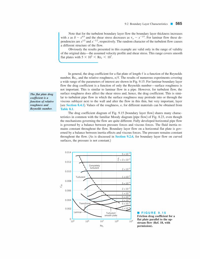
In general, the drag coefficient for a flat plate of length is a function of the Reynolds
number, and the relative roughness, The results of numerous experiments covering
a wide range of the parameters of interest are shown in Fig. 9.15. For laminar boundary layer
flow the drag coefficient is a function of only the Reynolds number—surface roughness is
not important. This is similar to laminar flow in a pipe. However, for turbulent flow, the
surface roughness does affect the shear stress and, hence, the drag coefficient. This is simi-
lar to turbulent pipe flow in which the surface roughness may protrude into or through the
viscous sublayer next to the wall and alter the flow in this thin, but very important, layer
1see Section 8.4.12. Values of the roughness, for different materials can be obtained from
Table 8.1.
The drag coefficient diagram of Fig. 9.15 1boundary layer flow2 shares many charac-
teristics in common with the familiar Moody diagram 1pipe flow2 of Fig. 8.23, even though
the mechanisms governing the flow are quite different. Fully developed horizontal pipe flow
is governed by a balance between pressure forces and viscous forces. The fluid inertia re-
mains constant throughout the flow. Boundary layer flow on a horizontal flat plate is gov-
erned by a balance between inertia effects and viscous forces. The pressure remains constant
throughout the flow. 1As is discussed in Section 9.2.6, for boundary layer flow on curved
surfaces, the pressure is not constant.2
e,
e//.Re/,
/
9.2 Boundary Layer Characteristics ■ 565
Note that for the turbulent boundary layer flow the boundary layer thickness increases
with x as and the shear stress decreases as For laminar flow these de-
pendencies are and respectively. The random character of the turbulent flow causes
a different structure of the flow.
Obviously the results presented in this example are valid only in the range of validity
of the original data—the assumed velocity profile and shear stress. This range covers smooth
flat plates with 5 3 1056 Re/ 6 107.
x21/2,x1/2
tw , x21/5.d , x4/5
0.002
0
0.004
0.006
0.008
0.010
0.012
105 106 107 108 109
Re,
CD
f
Turbulent
Completelyturbulent
1 × 10⁻³
2 × 10–3
= 3 × 10⁻³
5 × 10⁻³
ε
Laminar
5 × 10⁻⁴
2 × 10⁻⁴
1 × 10⁻⁴
5 × 10⁻⁵
5 × 10⁻⁶
1 × 10⁻⁶
Transitional
Turbulentsmooth plate
2 × 10⁻⁵
,
0.014
■ F I G U R E 9 . 1 5
Friction drag coefficient for aflat plate parallel to the up-stream flow (Ref. 18, withpermission).
The flat plate drag
coefficient is a
function of relative
roughness and
Reynolds number.

It is often convenient to have an equation for the drag coefficient as a function of the
Reynolds number and relative roughness rather than the graphical representation given in
Fig. 9.15. Although there is not one equation valid for the entire range, the equa-
tions presented in Table 9.3 do work well for the conditions indicated.
Re/ 2 e//
566 ■ Chapter 9 / Flow Over Immersed Bodies
Various equations
are available for
flat plate drag coef-
ficients.
■ TA B L E 9 . 3
Empirical Equations for the Flat Plate Drag Coefficient (Ref. 1)
Equation Flow Conditions
Laminar flow
Transitional with
Turbulent, smooth plate
Completely turbulentCDf 5 31.89 2 1.62 log1e//2 422.5
CDf 5 0.455/ 1log Re/22.58
Rexcr 5 5 3 105CDf 5 0.455/ 1log Re/22.58
2 1700/Re/
CDf 5 1.328/ 1Re/20.5
EXAMPLE
9.7
The water ski shown in Fig. E9.7a moves through water with a velocity U. Estimate
the drag caused by the shear stress on the bottom of the ski for
SOLUTION
Clearly the ski is not a flat plate, and it is not aligned exactly parallel to the upstream flow.
However, we can obtain a reasonable approximation to the shear force by using the flat plate
results. That is, the friction drag, caused by the shear stress on the bottom of the ski 1the
wall shear stress2 can be determined as
df 512rU
2/bCDf
df,
0 6 U 6 30 ft/s.
70 °F
00
1
2
3
4
5
5 10 15 20 25 30
1
2
3
4
5
U, ft /s
Entire boundarylayer laminar
xcr
$f
$f,
lb
x cr, ft
b = width = 0.5 ft
x = 0 x = 4 ft = ,U
x
(a)
(b)■ F I G U R E E 9 . 7

9.2 Boundary Layer Characteristics ■ 567
With and 1see
Table B.12 we obtain
(1)
where and U are in pounds and respectively.
The friction coefficient, can be obtained from Fig. 9.15 or from the appropriate
equations given in Table 9.3. As we will see, for this problem, much of the flow lies within
the transition regime where both the laminar and turbulent portions of the boundary layer
flow occupy comparable lengths of the plate. We choose to use the values of from the
table.
For the given conditions we obtain
where U is in With or we obtain from Table 9.3
From Eq. 1 the corresponding drag is
By covering the range of upstream velocities of interest we obtain the results shown in
Fig. E9.7b.
If the results of boundary layer theory are not valid—inertia effects are
not dominant enough and the boundary layer is not thin compared with the length of the
plate. For our problem this corresponds to For all practical purposes
U is greater than this value, and the flow past the ski is of the boundary layer type.
The approximate location of the transition from laminar to turbulent boundary layer
flow as defined by is indicated in Fig. E9.7b. Up to
the entire boundary layer is laminar. The fraction of the boundary layer that is laminar de-
creases as U increases until only the front 0.18 ft is laminar when
For anyone who has water skied, it is clear that it can require considerably more force
to be pulled along at than the 1two skis2 indicated in Fig. E9.7b.
As is discussed in Section 9.3, the total drag on an object such as a water ski consists of
more than just the friction drag. Other components, including pressure drag and wave-making
drag, add considerably to the total resistance.
2 3 4.88 lb 5 9.76 lb30 ft/s
U 5 30 ft/s.
U 5 1.31 ft/sRecr 5 rUxcr/m 5 5 3 105
U 5 2.63 3 1023 ft/s.
Re f 1000,
df 5 1.941102210.003082 5 0.598 lb
CDf 5 0.455/ 1log Re/22.58
2 1700/Re/ 5 0.00308.
Re/ 5 3.80 3 106,U 5 10 ft/s,ft/s.
Re/ 5rU/
m511.94 slugs/ft
32 14 ft2U
2.04 3 1025 lb # s/ft2
5 3.80 3 105 U
CDf
CDf,
ft/s,df
5 1.94 U 2CDf
df 512 11.94 slugs/ft
32 12.0 ft22U 2CDf
m 5 2.04 3 1025 lb # s/ft2A 5 /b 5 4 ft 3 0.5 ft 5 2 ft2, r 5 1.94 slugs/ft
3,
The free-stream ve-
locity on a curved
surface is not con-
stant.
9.2.6 Effects of Pressure Gradient
The boundary layer discussions in the previous parts of Section 9.2 have dealt with flow
along a flat plate in which the pressure is constant throughout the fluid. In general, when a
fluid flows past an object other than a flat plate, the pressure field is not uniform. As shown
in Fig. 9.6, if the Reynolds number is large, relatively thin boundary layers will develop along
the surfaces. Within these layers the component of the pressure gradient in the streamwise
direction 1i.e., along the body surface2 is not zero, although the pressure gradient normal to
the surface is negligibly small. That is, if we were to measure the pressure while moving
across the boundary layer from the body to the boundary layer edge, we would find that the
pressure is essentially constant. However, the pressure does vary in the direction along the
body surface if the body is curved. The variation in the free-stream velocity, the fluid
velocity at the edge of the boundary layer, is the cause of the pressure gradient in the bound-
ary layer. The characteristics of the entire flow 1both within and outside of the boundary
Ufs,

layer2 are often highly dependent on the pressure gradient effects on the fluid within the
boundary layer.
For a flat plate parallel to the upstream flow, the upstream velocity 1that far ahead of
the plate2 and the free-stream velocity 1that at the edge of the boundary layer2 are equal—
This is a consequence of the negligible thickness of the plate. For bodies of nonzero
thickness, these two velocities are different. This can be seen in the flow past a circular
cylinder of diameter D. The upstream velocity and pressure are U and respectively. If the
fluid were completely inviscid the Reynolds number would be infinite
and the streamlines would be symmetrical, as are shown in Fig. 9.16a. The
fluid velocity along the surface would vary from at the very front and rear of the
cylinder 1points A and F are stagnation points2 to a maximum of at the top and bot-
tom of the cylinder 1point C 2. The pressure on the surface of the cylinder would be sym-
metrical about the vertical midplane of the cylinder, reaching a maximum value of1the stagnation pressure2 at both the front and back of the cylinder, and a min-
imum of at the top and bottom of the cylinder. The pressure and free-stream
velocity distributions are shown in Figs. 9.16b and 9.16c. These characteristics can be ob-
tained from potential flow analysis of Section 6.6.3.
Because of the absence of viscosity 1therefore, 2 and the symmetry of the pres-
sure distribution for inviscid flow past a circular cylinder, it is clear that the drag on the cylin-
der is zero. Although it is not obvious, it can be shown that the drag is zero for any object
that does not produce a lift 1symmetrical or not2 in an inviscid fluid 1Ref. 42. Based on ex-
perimental evidence, however, we know that there must be a net drag. Clearly, since there is
no purely inviscid fluid, the reason for the observed drag must lie on the shoulders of the
viscous effects.
To test this hypothesis, we could conduct an experiment by measuring the drag on an
object 1such as a circular cylinder2 in a series of fluids with decreasing values of viscosity.
To our initial surprise we would find that no matter how small we make the viscosity 1pro-
tw 5 0
p0 2 3rU 2/2
p0 1 rU 2/2
Ufs 5 2U
Ufs 5 0
rUD/m 5 ` 2 1Re 51m 5 02, p0,
U 5 Ufs.
568 ■ Chapter 9 / Flow Over Immersed Bodies
If there were no
viscosity, there
would be no pres-
sure or friction
drag on a cylinder.
A F
C
θ
p0 + U 21
2
p0 – U 21
2
p0 – U 2
p0 – U 23
2
p0
p
2U
U
00 90 180
, degreesθ
0 90 180
, degreesθ
Ufs
U, p0
A
C
F
C
FA
Ufs
(a)
(b) (c)
ρ
ρ
ρ
ρ
■ F I G U R E 9 . 1 6
Inviscid flow past a circularcylinder: (a) streamlines for theflow if there were no viscous ef-fects, (b) pressure distributionon the cylinder’s surface,(c) free-stream velocity on thecylinder’s surface.
9.2 Boundary Layer Characteristics ■ 569
vided it is not precisely zero2 we would measure a finite drag, essentially independent of the
value of As was noted in Section 6.6.3, this leads to what has been termed d’Alembert’s
paradox—the drag on an object in an inviscid fluid is zero, but the drag on an object in a
fluid with vanishingly small 1but nonzero2 viscosity is not zero.
The reason for the above paradox can be described in terms of the effect of the pres-
sure gradient on boundary layer flow. Consider large Reynolds number flow of a real 1vis-
cous2 fluid past a circular cylinder. As was discussed in Section 9.1.2, we expect the viscous
effects to be confined to thin boundary layers near the surface. This allows the fluid to stick
to the surface—a necessary condition for any fluid, provided The basic idea
of boundary layer theory is that the boundary layer is thin enough so that it does not greatly
disturb the flow outside the boundary layer. Based on this reasoning, for large Reynolds num-
bers the flow throughout most of the flow field would be expected to be as is indicated in
Fig. 9.16a, the inviscid flow field.
The pressure distribution indicated in Fig. 9.16b is imposed on the boundary layer flow
along the surface of the cylinder. In fact, there is negligible pressure variation across the thin
boundary layer so that the pressure within the boundary layer is that given by the inviscid
flow field. This pressure distribution along the cylinder is such that the stationary fluid at the
nose of the cylinder is accelerated to its maximum velocity at
and then is decelerated back to zero velocity at the rear of the cylinder at
This is accomplished by a balance between pressure and inertia effects; viscous
effects are absent for the inviscid flow outside the boundary layer.
Physically, in the absence of viscous effects, a fluid particle traveling from the front to
the back of the cylinder coasts down the “pressure hill” from to 1from point
A to C in Fig. 9.16b2 and then back up the hill to 1from point C to F 2 without any
loss of energy. There is an exchange between kinetic and pressure energy, but there are no
energy losses. The same pressure distribution is imposed on the viscous fluid within the
boundary layer. The decrease in pressure in the direction of flow along the front half of the
cylinder is termed a favorable pressure gradient. The increase in pressure in the direction of
flow along the rear half of the cylinder is termed an adverse pressure gradient.
Consider a fluid particle within the boundary layer indicated in Fig. 9.17. In its attempt
to flow from A to F it experiences the same pressure distribution as the particles in the free
stream immediately outside the boundary layer—the inviscid flow field pressure. However, be-
cause of the viscous effects involved, the particle in the boundary layer experiences a loss of en-
ergy as it flows along. This loss means that the particle does not have enough energy to coast
all of the way up the pressure hill 1from C to F 2 and to reach point F at the rear of the cylinder.
This kinetic energy deficit is seen in the velocity profile detail at point C, shown in Fig. 9.17a.
Because of friction, the boundary layer fluid cannot travel from the front to the rear of the cylin-
der. 1This conclusion can also be obtained from the concept that due to viscous effects the par-
ticle at C does not have enough momentum to allow it to coast up the pressure hill to F.2The situation is similar to a bicyclist coasting down a hill and up the other side of the
valley. If there were no friction the rider starting with zero speed could reach the same height
from which he or she started. Clearly friction 1rolling resistance, aerodynamic drag, etc.2causes a loss of energy 1and momentum2, making it impossible for the rider to reach the
height from which he or she started without supplying additional energy 1i.e., peddling2. The
fluid within the boundary layer does not have such an energy supply. Thus, the fluid flows
against the increasing pressure as far as it can, at which point the boundary layer separates
from 1lifts off 2 the surface. This boundary layer separation is indicated in Fig. 9.17a. (See
the photograph at the beginning of Chapters 7, 9, and 11.) Typical velocity profiles at rep-
resentative locations along the surface are shown in Fig. 9.17b. At the separation location
1profile D2, the velocity gradient at the wall and the wall shear stress are zero. Beyond that
location 1from D to E 2 there is reverse flow in the boundary layer.
u 5 180°
u 5 90°u 5 0
u 5 180°2.1Ufs 5 0u 5 90°21Ufs 5 2U1Ufs 5 0 at u 5 02
m Þ 0.1V 5 02
m.
The pressure gradi-
ent in the external
flow is imposed
throughout the
boundary layer
fluid.
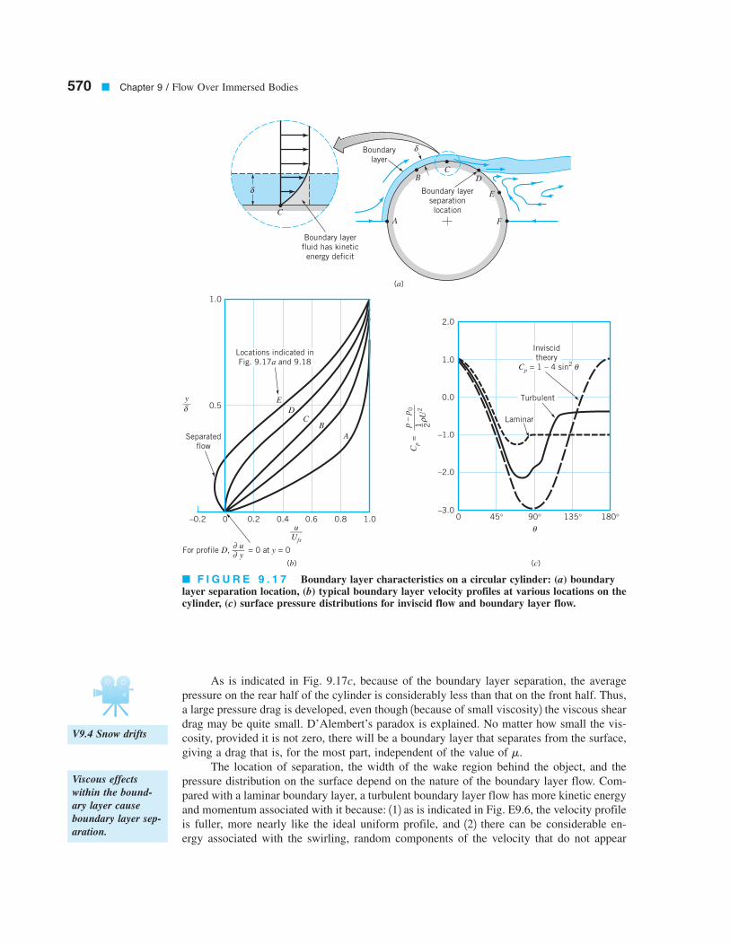
As is indicated in Fig. 9.17c, because of the boundary layer separation, the average
pressure on the rear half of the cylinder is considerably less than that on the front half. Thus,
a large pressure drag is developed, even though 1because of small viscosity2 the viscous shear
drag may be quite small. D’Alembert’s paradox is explained. No matter how small the vis-
cosity, provided it is not zero, there will be a boundary layer that separates from the surface,
giving a drag that is, for the most part, independent of the value of
The location of separation, the width of the wake region behind the object, and the
pressure distribution on the surface depend on the nature of the boundary layer flow. Com-
pared with a laminar boundary layer, a turbulent boundary layer flow has more kinetic energy
and momentum associated with it because: 112 as is indicated in Fig. E9.6, the velocity profile
is fuller, more nearly like the ideal uniform profile, and 122 there can be considerable en-
ergy associated with the swirling, random components of the velocity that do not appear
m.
570 ■ Chapter 9 / Flow Over Immersed Bodies
V9.4 Snow drifts
Viscous effects
within the bound-
ary layer cause
boundary layer sep-
aration.
■ F I G U R E 9 . 1 7 Boundary layer characteristics on a circular cylinder: (a) boundarylayer separation location, (b) typical boundary layer velocity profiles at various locations on thecylinder, (c) surface pressure distributions for inviscid flow and boundary layer flow.
Boundary layer
fluid has kinetic
energy deficit
C
δ
Boundary
layer
A
BC
D
E
F
Boundary layer
separation
location
δ
(a)
(b) (c)
Locations indicated in
Fig. 9.17a and 9.18
E
DC
B
A
1.0
0.5
0–0.2 0.2 0.4 0.6 0.8 1.0
Separated
flow
y__δ
u___Ufs
For profile D, = 0 at y = 0 u___
y
∂∂
2.0
1.0
0.0
–1.0
–2.0
–3.00 45° 90° 135° 180°
Laminar
Turbulent
Inviscid
theory
Cp = 1 – 4 sin2 θ
Cp =
p –
p0
____
___
U
21 _ 2
θ
ρ

in the time-averaged x component of velocity. Thus, as is indicated in Fig. 9.17c, the
turbulent boundary layer can flow farther around the cylinder 1farther up the pressure hill2before it separates than can the laminar boundary layer.
The structure of the flow field past a circular cylinder is completely different for a zero
viscosity fluid than it is for a viscous fluid, no matter how small the viscosity is, provided
it is not zero. This is due to boundary layer separation. Similar concepts hold for other shaped
bodies as well. The flow past an airfoil at zero angle of attack 1the angle between the up-
stream flow and the axis of the object2 is shown in Fig. 9.18a; flow past the same airfoil at
a angle of attack is shown in Fig. 9.18b. Over the front portion of the airfoil the pressure
decreases in the direction of flow—a favorable pressure gradient. Over the rear portion the
pressure increases in the direction of flow—an adverse pressure gradient. The boundary layer
velocity profiles at representative locations are similar to those indicated in Fig. 9.17b for
flow past a circular cylinder. If the adverse pressure gradient is not too great 1because the
body is not too “thick” in some sense2, the boundary layer fluid can flow into the slightly
increasing pressure region 1i.e., from C to the trailing edge in Fig. 9.18a2 without separating
from the surface. However, if the pressure gradient is too adverse 1because the angle of at-
tack is too large2, the boundary layer will separate from the surface as indicated in Fig. 9.18b.
Such situations can lead to the catastrophic loss of lift called stall, which is discussed in
Section 9.4.
Streamlined bodies are generally those designed to eliminate 1or at least to reduce2 the
effects of separation, whereas nonstreamlined bodies generally have relatively large drag due
to the low pressure in the separated regions 1the wake2. Although the boundary layer may be
quite thin, it can appreciably alter the entire flow field because of boundary layer separation.
These ideas are discussed in Section 9.3.
5°
9.2 Boundary Layer Characteristics ■ 571
Boundary layer
separation causes
airplane wings to
stall.
■ F I G U R E 9 . 1 8
Flow visualizationphotographs of flowpast an airfoil (theboundary layer veloc-ity profiles for thepoints indicated aresimilar to those indi-cated in Fig. 9.17b):(a) zero angle of at-tack, no separation,(b) angle of attack,flow separation. Dyein water. (Photographcourtesy of ONERA,France.)
58
9.2.7 Momentum-Integral Boundary Layer
Equation with Nonzero Pressure Gradient
The boundary layer results discussed in Sections 9.2.2 and 9.2.3 are valid only for boundary
layers with zero pressure gradients. They correspond to the velocity profile labeled C in
Fig. 9.17b. Boundary layer characteristics for flows with nonzero pressure gradients can be
obtained from nonlinear, partial differential boundary layer equations similar to Eqs. 9.8 and
9.9, provided the pressure gradient is appropriately accounted for. Such an approach is be-
yond the scope of this book 1Refs. 1, 22.An alternative approach is to extend the momentum integral boundary layer equation
technique 1Section 9.2.32 so that it is applicable for flows with nonzero pressure gradients.
The momentum integral equation for boundary layer flows with zero pressure gradient,
Eq. 9.26, is a statement of the balance between the shear force on the plate 1represented by
2 and rate of change of momentum of the fluid within the boundary layer [represented by
]. For such flows the free-stream velocity is constant If the free-
stream velocity is not constant [ where x is the distance measured along the
curved body], the pressure will not be constant. This follows from the Bernoulli equation
with negligible gravitational effects, since is constant along the streamlines out-
side the boundary layer. Thus,
(9.34)
For a given body the free-stream velocity and the corresponding pressure gradient on the sur-
face can be obtained from inviscid flow techniques 1potential flow2 discussed in Section 6.7.
1This is how the circular cylinder results of Fig. 9.16 were obtained.2Flow in a boundary layer with nonzero pressure gradient is very similar to that shown
in Fig. 9.11, except that the upstream velocity, U, is replaced by the free-stream velocity,
and the pressures at sections 112 and 122 are not necessarily equal. By using the x com-
ponent of the momentum equation 1Eq. 5.222 with the appropriate shear forces and pressure
forces acting on the control surface indicated in Fig. 9.11, the following integral momentum
equation for boundary layer flows is obtained:
(9.35)
The derivation of this equation is similar to that of the corresponding equation for constant-
pressure boundary layer flow, Eq. 9.26, although the inclusion of the pressure gradient effect
brings in additional terms 1Refs. 1, 2, 32. For example, both the boundary layer momentum
thickness, and the displacement thickness, are involved.
Equation 9.35, the general momentum integral equation for two-dimensional boundary
layer flow, represents a balance between viscous forces 1represented by 2, pressure forces
1represented by 2, and the fluid momentum 1represented by the
boundary layer momentum thickness2. In the special case of a flat plate, constant,
and Eq. 9.35 reduces to Eq. 9.26.
Equation 9.35 can be used to obtain boundary layer information in a manner similar
to that done for the flat plate boundary layer 1Section 9.2.32. That is, for a given body shape
the free-stream velocity, is determined, and a family of approximate boundary layer pro-
files is assumed. Equation 9.35 is then used to provide information about the boundary layer
thickness, wall shear stress, and other properties of interest. The details of this technique are
not within the scope of this book 1Refs. 1, 32.
Ufs,
Ufs 5 U 5
™,rUfs dUfs/dx 5 2dp/dx
tw
d*,™,
tw 5 r d
dx 1U 2
fs ™ 2 1 rd* Ufs dUfs
dx
Ufs1x2,
dp
dx5 2rUfs
dUfs
dx
p 1 rU2fs/2
Ufs 5 Ufs1x2,1Ufs 5 U2.rU 2 1d™/dx2
tw
572 ■ Chapter 9 / Flow Over Immersed Bodies
Pressure gradient
effects can be in-
cluded in the mo-
mentum integral
equation.
9.3 Drag
9.3 Drag ■ 573
As was discussed in Section 9.1, any object moving through a fluid will experience a drag,
—a net force in the direction of flow due to the pressure and shear forces on the surface
of the object. This net force, a combination of flow direction components of the normal and
tangential forces on the body, can be determined by use of Eqs. 9.1 and 9.2, provided the
distributions of pressure, p, and wall shear stress, are known. Only in very rare instances
can these distributions be determined analytically. The boundary layer flow past a flat plate
parallel to the upstream flow as is discussed in Section 9.2 is one such case. Current ad-
vances in computational fluid dynamics 1i.e., the use of computers to solve the governing
equations of the flow field2 have provided encouraging results for more complex shapes.
However, much work in this area remains.
Most of the information pertaining to drag on objects is a result of numerous experi-
ments with wind tunnels, water tunnels, towing tanks, and other ingenious devices that are
used to measure the drag on scale models. As was discussed in Chapter 7, these data can
be put into dimensionless form and the results can be appropriately ratioed for prototype cal-
culations. Typically, the result for a given-shaped object is a drag coefficient, where
(9.36)
and is a function of other dimensionless parameters such as Reynolds number, Re, Mach
number, Ma, Froude number, Fr, and relative roughness of the surface, That is,
The character of as a function of these parameters is discussed in this section.
9.3.1 Friction Drag
Friction drag, is that part of the drag that is due directly to the shear stress, on the
object. It is a function of not only the magnitude of the wall shear stress, but also of the ori-
entation of the surface on which it acts. This is indicated by the factor in Eq. 9.1. If
the surface is parallel to the upstream velocity, the entire shear force contributes directly to
the drag. This is true for the flat plate parallel to the flow as was discussed in Section 9.2.
If the surface is perpendicular to the upstream velocity, the shear stress contributes nothing
to the drag. Such is the case for a flat plate normal to the upstream velocity as was discussed
in Section 9.1.
In general, the surface of a body will contain portions parallel to and normal to the up-
stream flow, as well as any direction in between. A circular cylinder is such a body. Because
the viscosity of most common fluids is small, the contribution of the shear force to the over-
all drag on a body is often quite small. Such a statement should be worded in dimensionless
terms. That is, because the Reynolds number of most familiar flows is quite large, the per-
cent of the drag caused directly by the shear stress is often quite small. For highly stream-
lined bodies or for low Reynolds number flow, however, most of the drag may be due to fric-
tion drag.
The friction drag on a flat plate of width b and length oriented parallel to the up-
stream flow can be calculated from
where is the friction drag coefficient. The value of given as a function of Reynolds
number, and relative surface roughness, in Fig. 9.15 and Table 9.3, ise//,Re/ 5 rU//m,
CDf,CDf
df 512rU
2b/CDf
/
tw sin u
tw,df,
CD
CD 5 f1shape, Re, Ma, Fr, e//2
e//.
CD
CD 5d
12rU
2A
CD,
tw,
d
The drag coefficient
is a function of
other dimensionless
parameters.

a result of boundary layer analysis and experiments 1see Section 9.22. Typical values of
roughness, for various surfaces are given in Table 8.1. As with the pipe flow discussed in
Chapter 8, the flow is divided into two distinct categories—laminar or turbulent, with a tran-
sitional regime connecting them. The drag coefficient 1and, hence, the drag2 is not a function
of the plate roughness if the flow is laminar. However, for turbulent flow the roughness does
considerably affect the value of As with pipe flow, this dependence is a result of the sur-
face roughness elements protruding into or through the laminar sublayer 1see Section 8.32.Most objects are not flat plates parallel to the flow; instead, they are curved surfaces
along which the pressure varies. As was discussed in Section 9.2.6, this means that the bound-
ary layer character, including the velocity gradient at the wall, is different for most objects
from that for a flat plate. This can be seen in the change of shape of the boundary layer pro-
file along the cylinder in Fig. 9.17b.
The precise determination of the shear stress along the surface of a curved body is quite
difficult to obtain. Although approximate results can be obtained by a variety of techniques1Refs. 1, 22, these are outside the scope of this text. As is shown by the following example,
if the shear stress is known, its contribution to the drag can be determined.
CDf.
e,
574 ■ Chapter 9 / Flow Over Immersed Bodies
EXAMPLE
9.8
A viscous, incompressible fluid flows past the circular cylinder shown in Fig. E9.8a. Ac-
cording to a more advanced theory of boundary layer flow, the boundary layer remains at-
tached to the cylinder up to the separation location at with the dimensionless
wall shear stress as is indicated in Fig. E9.8b 1Ref. 12. The shear stress on the cylinder in the
wake region, is negligible. Determine the drag coefficient for the
cylinder based on the friction drag only.
SOLUTION
The friction drag, can be determined from Eq. 9.1 as
df 5 #tw sin u dA 5 2 aD
2b b #
p
0 tw sin u du
df,
CDf,108.8 6 u 6 180°,
u < 108.8°,
U θ θ
θ
Re = UD
_____ρµ
(a)
(b)
D
dA = b Dd
__
2
p dA
wdAτ
, degreesθ
Separation
θF = 0 for
> 108
1201008060402000
2
4
6
w R
eτ 1 _ 2
U2
ρF(
) ≡
____
___
θ
■ F I G U R E E 9 . 8
Friction (viscous)
drag is the drag
produced by viscous
shear stresses.

9.3.2 Pressure Drag
Pressure drag, is that part of the drag that is due directly to the pressure, p, on an object.
It is often referred to as form drag because of its strong dependency on the shape or form
of the object. Pressure drag is a function of the magnitude of the pressure and the orienta-
tion of the surface element on which the pressure force acts. For example, the pressure force
on either side of a flat plate parallel to the flow may be very large, but it does not contribute
to the drag because it acts in the direction normal to the upstream velocity. On the other
hand, the pressure force on a flat plate normal to the flow provides the entire drag.
dp,
9.3 Drag ■ 575
where b is the length of the cylinder. Note that is in radians 1not degrees2 to ensure the
proper dimensions of Thus,
This can be put into dimensionless form by using the dimensionless shear stress parameter,
given in Fig. E9.8b as follows:
where Thus,
(1)
The function obtained from Fig. E9.8b, is plotted in Fig. E9.8c. The necessary in-
tegration to obtain from Eq. 1 can be done by an appropriate numerical technique or by
an approximate graphical method to determine the area under the given curve.
The result is or
(Ans)
Note that the total drag must include both the shear stress 1friction2 drag and the pressure
drag. As we will see in Example 9.9, for the circular cylinder most of the drag is due to the
pressure force.
The above friction drag result is valid only if the boundary layer flow on the cylinder
is laminar. As is discussed in Section 9.3.3, for a smooth cylinder this means that
It is also valid only for flows that have a Reynolds number sufficiently
large to ensure the boundary layer structure to the flow. For the cylinder, this means Re 7 100.
rUD/m 6 3 3 105.
Re 5
CDf 55.93
1Re
ep0 F1u2 sin u du 5 5.93,
CDf
F1u2 sin u,
CDf 51
1Re #p
0
F1u2 sin u du
Re 5 rUD/m.
CDf 5 #p
0
tw
12rU
2 sin u du 5
1
1Re #p
0
tw 1Re
12rU
2 sin u du
F1u2 5 tw1Re/ 1rU 2/22,
CDf 5
df
12rU
2bD5
2
rU 2 #p
0
tw sin u du
dA 5 2 1D/22 b du.
u
ππ3___4
π __
2π __
40
0
2
4
6
, radθθ
θ(c)
F(
) si
n■ F I G U R E E 9 . 8 (Continued)
Pressure (form)
drag is the drag
produced by normal
stresses.

As previously noted, for most bodies, there are portions of the surface that are paral-
lel to the upstream velocity, others normal to the upstream velocity, and the majority of which
are at some angle in between. The pressure drag can be obtained from Eq. 9.1 provided a
detailed description of the pressure distribution and the body shape is given. That is,
which can be rewritten in terms of the pressure drag coefficient, as
(9.37)
Here is the pressure coefficient, where is a reference pressure.
The level of the reference pressure does not influence the drag directly because the net pres-
sure force on a body is zero if the pressure is constant 1i.e., 2 on the entire surface.
For flows in which inertial effects are large relative to viscous effects 1i.e., large
Reynolds number flows2, the pressure difference, scales directly with the dynamic
pressure, and the pressure coefficient is independent of Reynolds number. In such
situations we expect the drag coefficient to be relatively independent of Reynolds number.
For flows in which viscous effects are large relative to inertial effects 1i.e., very small
Reynolds number flows2, it is found that both the pressure difference and wall shear stress
scale with the characteristic viscous stress, where is a characteristic length. In such
situations we expect the drag coefficient to be proportional to That is,
These characteristics are similar to the
friction factor dependence of for laminar pipe flow and constant for large
Reynolds number flow 1see Section 8.42.If the viscosity were zero, the pressure drag on any shaped object 1symmetrical or not2 in
a steady flow would be zero. There perhaps would be large pressure forces on the front por-
tion of the object, but there would be equally large 1and oppositely directed2 pressure forces
on the rear portion. If the viscosity is not zero, the net pressure drag may be nonzero be-
cause of boundary layer separation as is discussed in Section 9.2.6. Example 9.9 illustrates
this.
f ,f , 1/ Re
d/ 1rU 2/22 , 1mU//2/ 1rU 2
/22 , m/rU/ 5 1/Re.
CD ,1/Re.
/mU//,
rU 2/2,
p 2 p0,
p0
p0Cp 5 1 p 2 p02/ 1rU 2/22
CDp 5
dp
12rU
2A5
# p cos u dA
12rU
2A5
#Cp cos u dA
A
CDp,
dp 5 # p cos u dA
576 ■ Chapter 9 / Flow Over Immersed Bodies
EXAMPLE
9.9
A viscous, incompressible fluid flows past the circular cylinder shown in Fig. E9.8a. The
pressure coefficient on the surface of the cylinder 1as determined from experimental mea-
surements2 is as indicated in Fig. E9.9a. Determine the pressure drag coefficient for this flow.
Combine the results of Examples 9.8 and 9.9 to determine the drag coefficient for a circu-
lar cylinder. Compare your results with those given in Fig. 9.21.
SOLUTION
The pressure 1form2 drag coefficient, can be determined from Eq. 9.37 as
or because of symmetry
CDp 5 #p
0
Cp cos u du
CDp 51
A # Cp cos u dA 5
1
bD #
2p
0
Cp cos u b aD
2b du
CDp,
The pressure coeffi-
cient is a dimen-
sionless form of the
pressure.
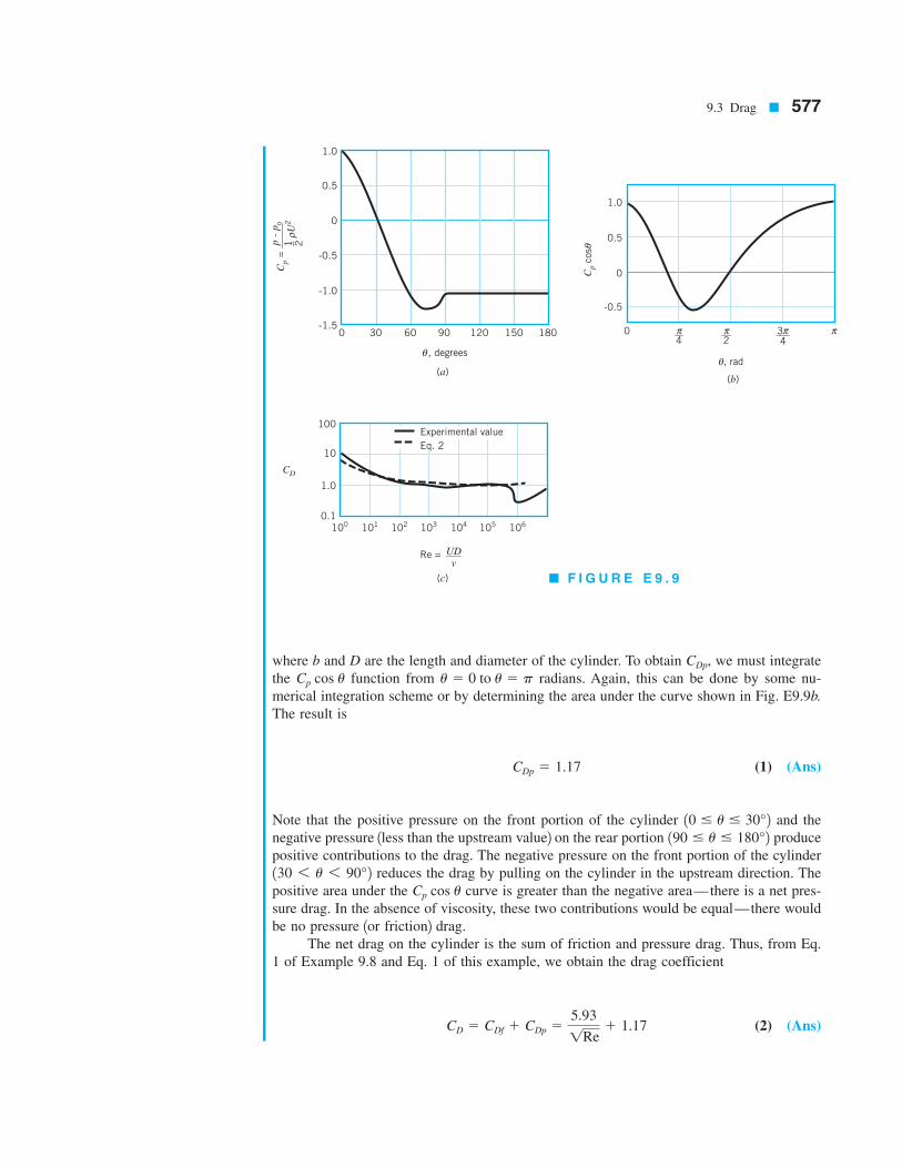
9.3 Drag ■ 577
where b and D are the length and diameter of the cylinder. To obtain we must integrate
the function from radians. Again, this can be done by some nu-
merical integration scheme or by determining the area under the curve shown in Fig. E9.9b.
The result is
(1) (Ans)
Note that the positive pressure on the front portion of the cylinder and the
negative pressure 1less than the upstream value2 on the rear portion produce
positive contributions to the drag. The negative pressure on the front portion of the cylinder
reduces the drag by pulling on the cylinder in the upstream direction. The
positive area under the curve is greater than the negative area—there is a net pres-
sure drag. In the absence of viscosity, these two contributions would be equal—there would
be no pressure 1or friction2 drag.
The net drag on the cylinder is the sum of friction and pressure drag. Thus, from Eq.
1 of Example 9.8 and Eq. 1 of this example, we obtain the drag coefficient
(2) (Ans)CD 5 CDf 1 CDp 55.93
1Re1 1.17
Cp cos u
130 6 u 6 90°2
190 # u # 180°210 # u # 30°2
CDp 5 1.17
u 5 0 to u 5 pCp cos u
CDp,
Experimental value
Eq. 2
1061051041031021011000.1
1.0
10
100
Re = UD___v
(c)
(a)(b)
CD
0-1.5
-1.0
-0.5
0
0.5
1.0
30 60 90 120 150 180
θ , degrees
Cp =
_____
p -
po
1 _ 2U
2ρ
ππ3 ___4
π__2
π__4
0
-0.5
0
0.5
1.0
, rad
θ
θ
Cp c
os
■ F I G U R E E 9 . 9

9.3.3 Drag Coefficient Data and Examples
As was discussed in previous sections, the net drag is produced by both pressure and shear
stress effects. In most instances these two effects are considered together, and an overall drag
coefficient, as defined in Eq. 9.36 is used. There is an abundance of such drag coeffi-
cient data available in the literature. This information covers incompressible and compress-
ible viscous flows past objects of almost any shape of interest—both man-made and natural
objects. In this section we consider a small portion of this information for representative sit-
uations. Additional data can be obtained from various sources 1Refs. 5, 62.Shape Dependence. Clearly the drag coefficient for an object depends on the shape
of the object, with shapes ranging from those that are streamlined to those that are blunt. The
drag on an ellipse with aspect ratio where D and are the thickness and length paral-
lel to the flow, illustrates this dependence. The drag coefficient based
on the frontal area, where b is the length normal to the flow, is as shown in Fig. 9.19.
The more blunt the body, the larger the drag coefficient. With 1i.e., a flat plate
normal to the flow2 we obtain the flat plate value of With the corre-
sponding value for a circular cylinder is obtained. As becomes larger the value of
decreases.
For very large aspect ratios the ellipse behaves as a flat plate parallel to the
flow. For such cases, the friction drag is greater than the pressure drag, and the value of
based on the frontal area, would increase with increasing 1This occurs for
larger values than those shown in the figure.2 For such extremely thin bodies 1i.e., an el-
lipse with a flat plate, or very thin airfoils2 it is customary to use the planform
area, in defining the drag coefficient. After all, it is the planform area on which the
shear stress acts, rather than the much smaller 1for thin bodies2 frontal area. The ellipse drag
coefficient based on the planform area, is also shown in Fig. 9.19. Clearly
the drag obtained by using either of these drag coefficients would be the same. They merely
represent two different ways to package the same information.
The amount of streamlining can have a considerable effect on the drag. Incredibly, the
drag on the two two-dimensional objects drawn to scale in Fig. 9.20 is the same. The width
of the wake for the streamlined strut is very thin, on the order of that for the much smaller
diameter circular cylinder.
CD 5 d/ 1rU 2b//22,A 5 b/,
//DS`,
//D
//D.A 5 bD,
CD
1//DS`2CD//D
//D 5 1CD 5 1.9.
//D 5 0
A 5 bD,
CD 5 d/ 1rU 2 bD/22,///D,
CD,
578 ■ Chapter 9 / Flow Over Immersed Bodies
This result is compared with the standard experimental value 1obtained from Fig. 9.212 in
Fig. E9.9c. The agreement is very good over a wide range of Reynolds numbers. For
the curves diverge because the flow is not a boundary layer type flow—the shear stress and
pressure distributions used to obtain Eq. 2 are not valid in this range. The drastic divergence
in the curves for is due to the change from a laminar to turbulent bound-
ary layer, with the corresponding change in the pressure distribution. This is discussed in
Section 9.3.3.
It is of interest to compare the friction drag to the total drag on the cylinder. That is,
For and this ratio is 0.138, 0.0483, and 0.0158, respectively. Most of the
drag on the blunt cylinder is pressure drag—a result of the boundary layer separation.
105Re 5 103, 104,
df
d5
CDf
CD
55.93/1Re
15.93/1Re2 1 1.175
1
1 1 0.1971Re
Re 7 3 3 105
Re 6 10
V9.5 Skydiving
practice
The drag coefficient
may be based on
the frontal area or
the planform area.
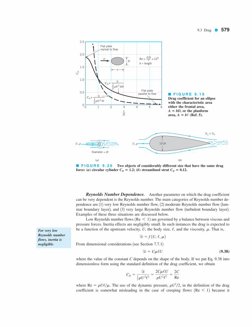
Reynolds Number Dependence. Another parameter on which the drag coefficient
can be very dependent is the Reynolds number. The main categories of Reynolds number de-
pendence are 112 very low Reynolds number flow, 122 moderate Reynolds number flow 1lam-
inar boundary layer2, and 132 very large Reynolds number flow 1turbulent boundary layer2.Examples of these three situations are discussed below.
Low Reynolds number flows are governed by a balance between viscous and
pressure forces. Inertia effects are negligibly small. In such instances the drag is expected to
be a function of the upstream velocity, U, the body size, and the viscosity, That is,
From dimensional considerations 1see Section 7.7.12(9.38)
where the value of the constant C depends on the shape of the body. If we put Eq. 9.38 into
dimensionless form using the standard definition of the drag coefficient, we obtain
where The use of the dynamic pressure, in the definition of the drag
coefficient is somewhat misleading in the case of creeping flows because it 1Re 6 12rU2/2,Re 5 rU//m.
CD 5d
12rU
2/
25
2Cm/U
rU 2/
25
2C
Re
d 5 Cm/U
d 5 f 1U, /, m2m./,
1Re 6 12
9.3 Drag ■ 579
For very low
Reynolds number
flows, inertia is
negligible.
■ F I G U R E 9 . 2 0 Two objects of considerably different size that have the same dragforce: (a) circular cylinder (b) streamlined strut CD 5 0.12.CD 5 1.2;
■ F I G U R E 9 . 1 9
Drag coefficient for an ellipsewith the characteristic areaeither the frontal area,
or the planformarea, (Ref. 5).A 5 b/A 5 bD,
2.5
2.0
1.5
1.0
0.5
00 1 2 3 4 5 6
DU
Flat plateparallel to flow
D
CD
Re = = 105UDv
b = length
U2 bD1
2
CD =
•
U2 b1
2
CD =
Flat platenormal to flow
,
$
$
ρ ,
ρ
,
U, ρU, ρ
Diameter = D
(a) (b)
10 D
$a = $b
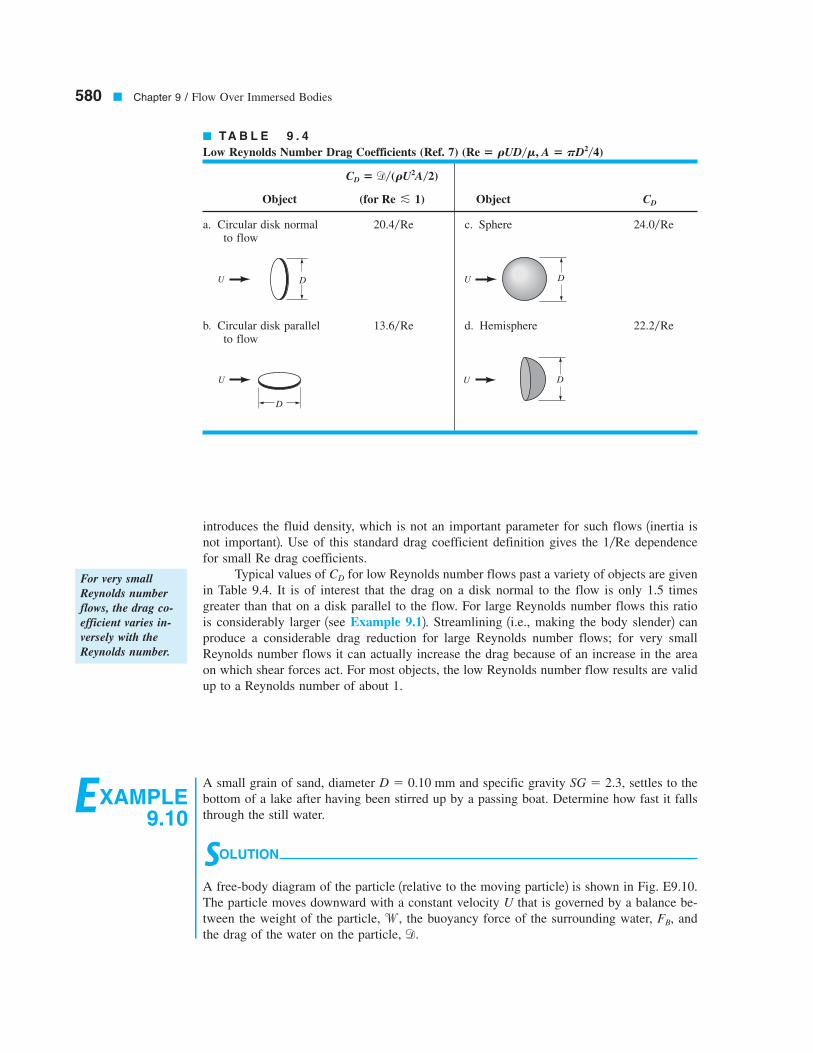
introduces the fluid density, which is not an important parameter for such flows 1inertia is
not important2. Use of this standard drag coefficient definition gives the dependence
for small Re drag coefficients.
Typical values of for low Reynolds number flows past a variety of objects are given
in Table 9.4. It is of interest that the drag on a disk normal to the flow is only 1.5 times
greater than that on a disk parallel to the flow. For large Reynolds number flows this ratio
is considerably larger 1see Example 9.12. Streamlining 1i.e., making the body slender2 can
produce a considerable drag reduction for large Reynolds number flows; for very small
Reynolds number flows it can actually increase the drag because of an increase in the area
on which shear forces act. For most objects, the low Reynolds number flow results are valid
up to a Reynolds number of about 1.
CD
1/Re
580 ■ Chapter 9 / Flow Over Immersed Bodies
■ TA B L E 9 . 4
Low Reynolds Number Drag Coefficients (Ref. 7) ( )
( )
Object ( ) Object
a. Circular disk normal c. Sphereto flow
b. Circular disk parallel d. Hemisphereto flow
22.2/Re13.6/Re
24.0/Re20.4/Re
CDfor Re f 1
RU2A/2CD 5 d/
Re 5 RUD/M, A 5 PD2/4
U D
U
D
U D
U D
For very small
Reynolds number
flows, the drag co-
efficient varies in-
versely with the
Reynolds number.
EXAMPLE
9.10
A small grain of sand, diameter and specific gravity settles to the
bottom of a lake after having been stirred up by a passing boat. Determine how fast it falls
through the still water.
SOLUTION
A free-body diagram of the particle 1relative to the moving particle2 is shown in Fig. E9.10.
The particle moves downward with a constant velocity U that is governed by a balance be-
tween the weight of the particle, the buoyancy force of the surrounding water, and
the drag of the water on the particle, d.
FB,w,
SG 5 2.3,D 5 0.10 mm
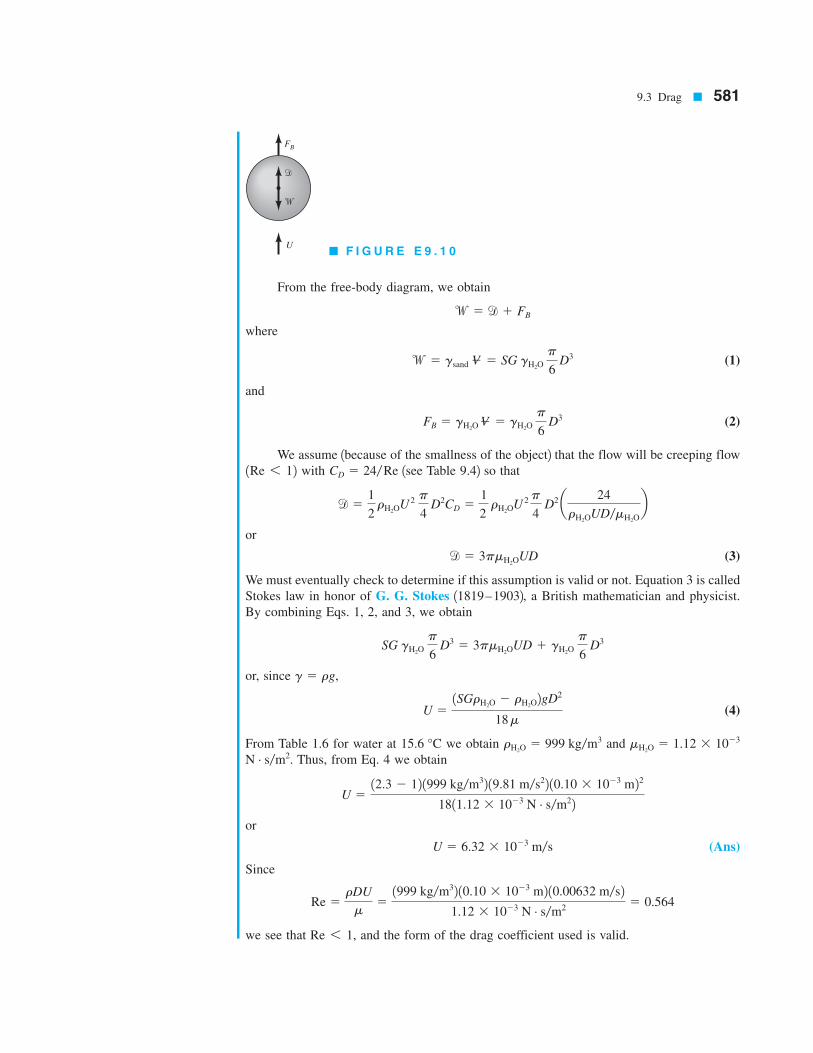
9.3 Drag ■ 581
FB
$
0
U
From the free-body diagram, we obtain
where
(1)
and
(2)
We assume 1because of the smallness of the object2 that the flow will be creeping flow
with 1see Table 9.42 so that
or
(3)
We must eventually check to determine if this assumption is valid or not. Equation 3 is called
Stokes law in honor of G. G. Stokes 11819–19032, a British mathematician and physicist.
By combining Eqs. 1, 2, and 3, we obtain
or, since
(4)
From Table 1.6 for water at we obtain and
Thus, from Eq. 4 we obtain
or
(Ans)
Since
we see that and the form of the drag coefficient used is valid.Re 6 1,
Re 5rDU
m51999 kg/m
32 10.10 3 1023 m2 10.00632 m/s21.12 3 1023 N # s/m
25 0.564
U 5 6.32 3 1023 m/s
U 512.3 2 12 1999 kg/m
32 19.81 m/s22 10.10 3 1023 m22
1811.12 3 1023 N # s/m22
N # s/m2.
mH2O5 1.12 3 1023rH2O
5 999 kg/m315.6 °C
U 5
1SGrH2O2 rH2O
2gD2
18 m
g 5 rg,
SG gH2O p
6 D3
5 3pmH2OUD 1 gH2O
p
6 D3
d 5 3pmH2OUD
d 51
2 rH2O
U 2 p
4 D2CD 5
1
2
rH2OU 2
p
4 D2
a 24
rH2OUD/mH2O
bCD 5 24/Re1Re 6 12
FB 5 gH2O V2 5 gH2O p
6 D3
w 5 gsand V2 5 SG gH2O p
6 D3
w 5 d 1 FB
■ F I G U R E E 9 . 1 0
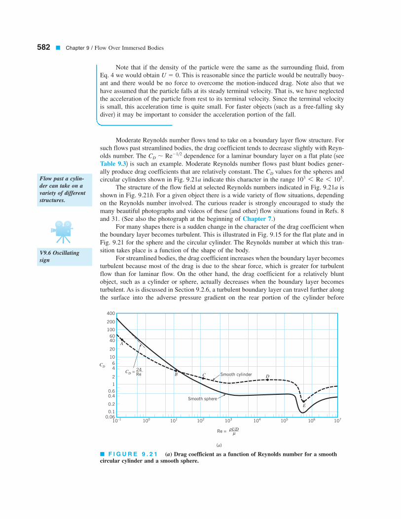
Moderate Reynolds number flows tend to take on a boundary layer flow structure. For
such flows past streamlined bodies, the drag coefficient tends to decrease slightly with Reyn-
olds number. The dependence for a laminar boundary layer on a flat plate 1see
Table 9.32 is such an example. Moderate Reynolds number flows past blunt bodies gener-
ally produce drag coefficients that are relatively constant. The values for the spheres and
circular cylinders shown in Fig. 9.21a indicate this character in the range
The structure of the flow field at selected Reynolds numbers indicated in Fig. 9.21a is
shown in Fig. 9.21b. For a given object there is a wide variety of flow situations, depending
on the Reynolds number involved. The curious reader is strongly encouraged to study the
many beautiful photographs and videos of these 1and other2 flow situations found in Refs. 8
and 31. (See also the photograph at the beginning of Chapter 7.)
For many shapes there is a sudden change in the character of the drag coefficient when
the boundary layer becomes turbulent. This is illustrated in Fig. 9.15 for the flat plate and in
Fig. 9.21 for the sphere and the circular cylinder. The Reynolds number at which this tran-
sition takes place is a function of the shape of the body.
For streamlined bodies, the drag coefficient increases when the boundary layer becomes
turbulent because most of the drag is due to the shear force, which is greater for turbulent
flow than for laminar flow. On the other hand, the drag coefficient for a relatively blunt
object, such as a cylinder or sphere, actually decreases when the boundary layer becomes
turbulent. As is discussed in Section 9.2.6, a turbulent boundary layer can travel further along
the surface into the adverse pressure gradient on the rear portion of the cylinder before
1036 Re 6 105.
CD
CD , Re21/2
582 ■ Chapter 9 / Flow Over Immersed Bodies
Note that if the density of the particle were the same as the surrounding fluid, from
Eq. 4 we would obtain This is reasonable since the particle would be neutrally buoy-
ant and there would be no force to overcome the motion-induced drag. Note also that we
have assumed that the particle falls at its steady terminal velocity. That is, we have neglected
the acceleration of the particle from rest to its terminal velocity. Since the terminal velocity
is small, this acceleration time is quite small. For faster objects 1such as a free-falling sky
diver2 it may be important to consider the acceleration portion of the fall.
U 5 0.
Flow past a cylin-
der can take on a
variety of different
structures.
V9.6 Oscillating
sign
■ F I G U R E 9 . 2 1 (a) Drag coefficient as a function of Reynolds number for a smoothcircular cylinder and a smooth sphere.
A
B C D
E
Smooth cylinder
Smooth sphere
CD = 24
___
Re
400
200
100
6040
20
10
64
2
1
0.60.4
0.2
0.1
0.0610–1 100 101 102 103 104 105 106 107
Re = UD
____ρµ
(a)
CD
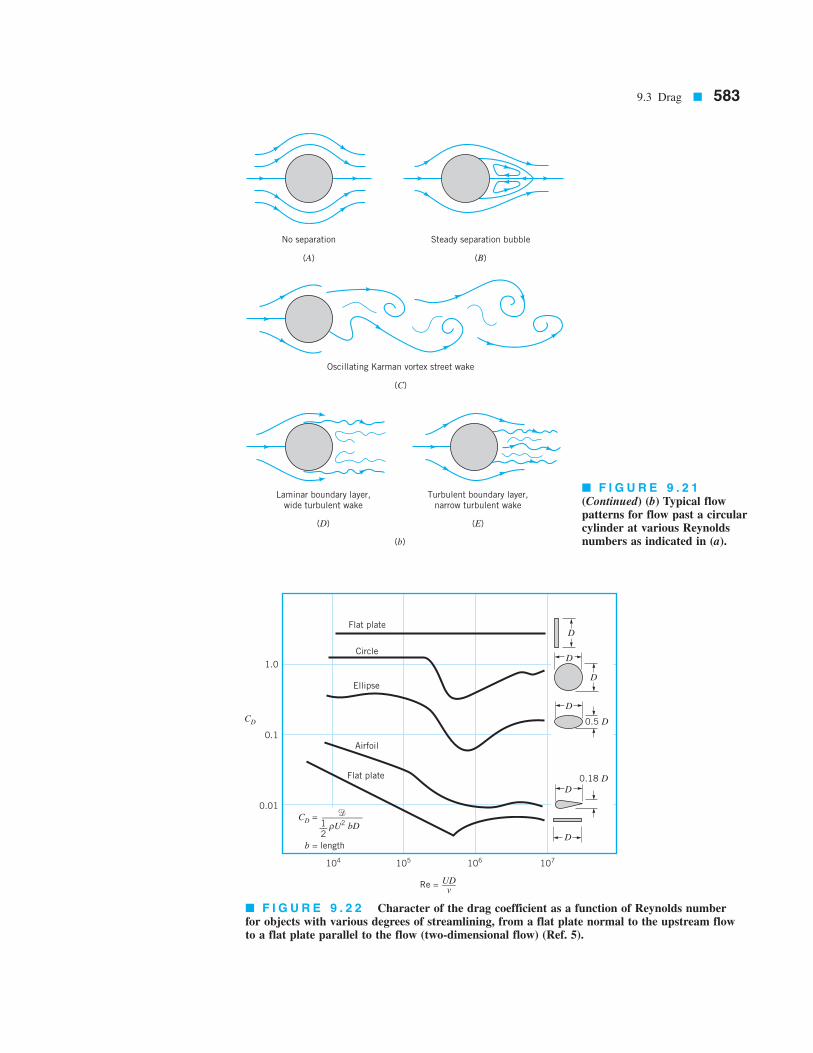
9.3 Drag ■ 583
No separation
(A)
Steady separation bubble
(B)
Oscillating Karman vortex street wake
(C)
Laminar boundary layer,
wide turbulent wake
(D)
Turbulent boundary layer,
narrow turbulent wake
(E)
(b)
Flat plate
Circle
Ellipse
Airfoil
Flat plate
CD =$_________
U2
bD1__
2ρ
D
D
0.18 D
0.5 D
D
D
D
D
1.0
0.1
0.01
CD
104 105 106 107
Re = UD___v
b = length
■ F I G U R E 9 . 2 1
(Continued) (b) Typical flowpatterns for flow past a circularcylinder at various Reynoldsnumbers as indicated in (a).
■ F I G U R E 9 . 2 2 Character of the drag coefficient as a function of Reynolds numberfor objects with various degrees of streamlining, from a flat plate normal to the upstream flowto a flat plate parallel to the flow (two-dimensional flow) (Ref. 5).

separation occurs. The result is a thinner wake and smaller pressure drag for turbulent bound-
ary layer flow. This is indicated in Fig. 9.21 by the sudden decrease in for
In a portion of this range the actual drag 1not just the drag coefficient2 de-
creases with increasing speed. It would be very difficult to control the steady flight of such
an object in this range—an increase in velocity requires a decrease in thrust 1drag2. In all
other Reynolds number ranges the drag increases with an increase in the upstream velocity1even though may decrease with Re2.For extremely blunt bodies, like a flat plate perpendicular to the flow, the flow sepa-
rates at the edge of the plate regardless of the nature of the boundary layer flow. Thus, the
drag coefficient shows very little dependence on the Reynolds number.
The drag coefficients for a series of two-dimensional bodies of varying bluntness are
given as a function of Reynolds number in Fig. 9.22. The characteristics described above are
evident.
CD
1056 Re 6 106.
CD
584 ■ Chapter 9 / Flow Over Immersed Bodies
The drag coefficient
may change consid-
erably when the
boundary layer be-
comes turbulent.
EXAMPLE
9.11
Hail is produced by the repeated rising and falling of ice particles in the updraft of a thun-
derstorm, as is indicated in Fig. E9.11. When the hail becomes large enough, the aerody-
namic drag from the updraft can no longer support the weight of the hail, and it falls from
the storm cloud. Estimate the velocity, U, of the updraft needed to make -in.-diameter1i.e., “golf ball-sized”2 hail.
D 5 1.5
SOLUTION
As is discussed in Example 9.10, for steady-state conditions a force balance on an object
falling through a fluid gives
where is the buoyant force of the air on the particle, is the particle
weight, and is the aerodynamic drag. This equation can be rewritten as
(1)
With and since 1i.e., 2, Eq. 1 can be simplified to
(2)
By using and
Eq. 2 becomes
or
(3)U 564.5
1CD
U 5 c 411.84 slugs/ft32 132.2 ft/s
22 10.125 ft2312.38 3 1023 slugs/ft
32CD
d 1/2
D 5 1.5 in. 5 0.125 ft,rice 5 1.84 slugs/ft3, rair 5 2.38 3 1023 slugs/ft
3,
U 5 a4
3
rice
rair
gD
CD
b1/2
w @ FBgice @ gairV2 5 pD3/6
12rairU
2 p
4 D2CD 5w 2 FB
d
w 5 gice V2FB 5 gair V2
w 5 d 1 FB
Anvil
Storm
movement
Ground
HailUpdraft
Rain
40,000
to
50,000 ftDowndraft
■ F I G U R E E 9 . 1 1
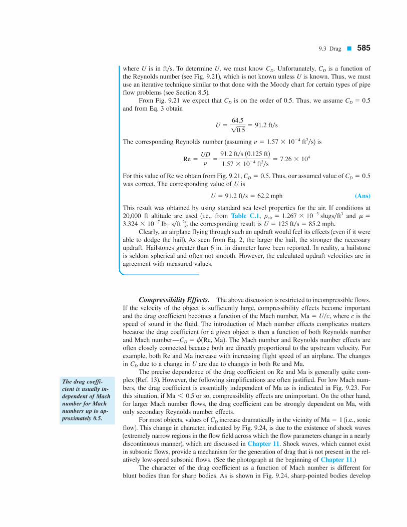
Compressibility Effects. The above discussion is restricted to incompressible flows.
If the velocity of the object is sufficiently large, compressibility effects become important
and the drag coefficient becomes a function of the Mach number, where c is the
speed of sound in the fluid. The introduction of Mach number effects complicates matters
because the drag coefficient for a given object is then a function of both Reynolds number
and Mach number— The Mach number and Reynolds number effects are
often closely connected because both are directly proportional to the upstream velocity. For
example, both Re and Ma increase with increasing flight speed of an airplane. The changes
in due to a change in U are due to changes in both Re and Ma.
The precise dependence of the drag coefficient on Re and Ma is generally quite com-
plex 1Ref. 132. However, the following simplifications are often justified. For low Mach num-
bers, the drag coefficient is essentially independent of Ma as is indicated in Fig. 9.23. For
this situation, if or so, compressibility effects are unimportant. On the other hand,
for larger Mach number flows, the drag coefficient can be strongly dependent on Ma, with
only secondary Reynolds number effects.
For most objects, values of increase dramatically in the vicinity of 1i.e., sonic
flow2. This change in character, indicated by Fig. 9.24, is due to the existence of shock waves
1extremely narrow regions in the flow field across which the flow parameters change in a nearly
discontinuous manner2, which are discussed in Chapter 11. Shock waves, which cannot exist
in subsonic flows, provide a mechanism for the generation of drag that is not present in the rel-
atively low-speed subsonic flows. (See the photograph at the beginning of Chapter 11.)
The character of the drag coefficient as a function of Mach number is different for
blunt bodies than for sharp bodies. As is shown in Fig. 9.24, sharp-pointed bodies develop
Ma 5 1CD
Ma 6 0.5
CD
CD 5 f1Re, Ma2.
Ma 5 U/c,
9.3 Drag ■ 585
The drag coeffi-
cient is usually in-
dependent of Mach
number for Mach
numbers up to ap-
proximately 0.5.
where U is in To determine U, we must know Unfortunately, is a function of
the Reynolds number 1see Fig. 9.212, which is not known unless U is known. Thus, we must
use an iterative technique similar to that done with the Moody chart for certain types of pipe
flow problems 1see Section 8.52.From Fig. 9.21 we expect that is on the order of 0.5. Thus, we assume
and from Eq. 3 obtain
The corresponding Reynolds number 1assuming 2 is
For this value of Re we obtain from Fig. 9.21, Thus, our assumed value of
was correct. The corresponding value of U is
(Ans)
This result was obtained by using standard sea level properties for the air. If conditions at
20,000 ft altitude are used 1i.e., from Table C.1, and
2, the corresponding result is
Clearly, an airplane flying through such an updraft would feel its effects 1even if it were
able to dodge the hail2. As seen from Eq. 2, the larger the hail, the stronger the necessary
updraft. Hailstones greater than 6 in. in diameter have been reported. In reality, a hailstone
is seldom spherical and often not smooth. However, the calculated updraft velocities are in
agreement with measured values.
U 5 125 ft/s 5 85.2 mph.3.324 3 1027 lb # s/ft 2
m 5rair 5 1.267 3 1023 slugs/ft3
U 5 91.2 ft/s 5 62.2 mph
CD 5 0.5CD 5 0.5.
Re 5UD
n5
91.2 ft/s 10.125 ft2
1.57 3 1024 ft2/s
5 7.26 3 104
n 5 1.57 3 1024 ft2/s
U 564.5
10.55 91.2 ft/s
CD 5 0.5CD
CDCD.ft/s.
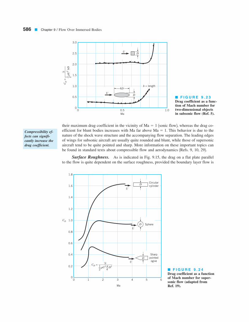
their maximum drag coefficient in the vicinity of 1sonic flow2, whereas the drag co-
efficient for blunt bodies increases with Ma far above This behavior is due to the
nature of the shock wave structure and the accompanying flow separation. The leading edges
of wings for subsonic aircraft are usually quite rounded and blunt, while those of supersonic
aircraft tend to be quite pointed and sharp. More information on these important topics can
be found in standard texts about compressible flow and aerodynamics 1Refs. 9, 10, 292.
Surface Roughness. As is indicated in Fig. 9.15, the drag on a flat plate parallel
to the flow is quite dependent on the surface roughness, provided the boundary layer flow is
Ma 5 1.
Ma 5 1
586 ■ Chapter 9 / Flow Over Immersed Bodies
■ F I G U R E 9 . 2 3
Drag coefficient as a func-tion of Mach number fortwo-dimensional objects in subsonic flow (Ref. 5).
■ F I G U R E 9 . 2 4
Drag coefficient as a functionof Mach number for super-sonic flow (adapted from Ref. 19).
4D
UD
UD
0.5 1.0
b = length
0
Ma
3.0
2.5
2.0
1.5
1.0
0.5
0
CD =
$__
____
____
U2 b
D1 __ 2
ρ
U
U
U
Circular
cylinderD
SphereD
Sharp
pointed
ogiveD
CD =$___________
U2
D21__2
__4
π
0 1 2 3 4 5 6
Ma
0
0.2
0.4
0.6
0.8
1.0
1.2
1.4
1.6
1.8
CD
ρ
Compressibility ef-
fects can signifi-
cantly increase the
drag coefficient.

turbulent. In such cases the surface roughness protrudes through the laminar sublayer adja-
cent to the surface 1see Section 8.42 and alters the wall shear stress. In addition to the in-
creased turbulent shear stress, surface roughness can alter the Reynolds number at which the
boundary layer flow becomes turbulent. Thus, a rough flat plate may have a larger portion
of its length covered by a turbulent boundary layer than does the corresponding smooth plate.
This also acts to increase the net drag on the plate.
In general, for streamlined bodies, the drag increases with increasing surface rough-
ness. Great care is taken to design the surfaces of airplane wings to be as smooth as possi-
ble, since protruding rivets or screw heads can cause a considerable increase in the drag. On
the other hand, for an extremely blunt body, such as a flat plate normal to the flow, the drag
is independent of the surface roughness, since the shear stress is not in the upstream flow di-
rection and contributes nothing to the drag.
For blunt bodies like a circular cylinder or sphere, an increase in surface roughness can
actually cause a decrease in the drag. This is illustrated for a sphere in Fig. 9.25. As is dis-
cussed in Section 9.2.6, when the Reynolds number reaches the critical value 1for a smooth sphere2, the boundary layer becomes turbulent and the wake region behind the
sphere becomes considerably narrower than if it were laminar 1see Fig. 9.172. The result is a
considerable drop in pressure drag with a slight increase in friction drag, combining to give
a smaller overall drag 1and 2.The boundary layer can be tripped into turbulence at a smaller Reynolds number by
using a rough-surfaced sphere. For example, the critical Reynolds number for a golf ball is
approximately In the range the drag on the stan-
dard rough 1i.e., dimpled2 golf ball is considerably less
than for the smooth ball. As is shown in Example 9.12, this is precisely the Reynolds num-
ber range for well-hit golf balls—hence, the reason for dimples on golf balls. The Reynolds
number range for well-hit table tennis balls is less than Thus, table tennis
balls are smooth.
Re 5 4 3 104.
1DDrough/CDsmooth < 0.25/0.5 5 0.524 3 104
6 Re 6 4 3 105,Re 5 4 3 104.
CD
Re 5 3 3 105
9.3 Drag ■ 587
■ F I G U R E 9 . 2 5 The effect of surface roughness on the drag coefficient of a sphere inthe Reynolds number range for which the laminar boundary layer becomes turbulent (Ref. 5).
0.6
0.5
0.4
0.3
0.2
0.1
04 × 104 105 106 4 × 10⁵ 4 × 10⁶
Re = UD
___v
Golf
ball
CD =
$__
____
____
_
U
2
D
21 __ 2
__ 4π
ε__D
ε__D
ε__D
ε__D
ε__D
= 5 × 10–3
= 1.25 × 10–2
= 0 (smooth)
= relative roughness
ρ
= 1.5 × 10⁻³
Depending on the
body shape, an in-
crease in surface
roughness may in-
crease or decrease
drag.

588 ■ Chapter 9 / Flow Over Immersed Bodies
EXAMPLE
9.12
A well-hit golf ball 1diameter in., weight 2 can travel at
as it leaves the tee. A well-hit table tennis ball 1diameter weight
can travel at as it leaves the paddle. Determine the drag on a standard golf ball,
a smooth golf ball, and a table tennis ball for the conditions given. Also determine the de-
celeration of each ball for these conditions.
SOLUTION
For either ball, the drag can be obtained from
(1)
where the drag coefficient, is given in Fig. 9.25 as a function of the Reynolds number
and surface roughness. For the golf ball in standard air
while for the table tennis ball
The corresponding drag coefficients are for the standard golf ball, for
the smooth golf ball, and for the table tennis ball. Hence, from Eq. 1 for the stan-
dard golf ball
(Ans)
for the smooth golf ball
(Ans)
and for the table tennis ball
(Ans)
The corresponding decelerations are where m is the mass of the
ball. Thus, the deceleration relative to the acceleration of gravity, 1i.e., the number of g’s
deceleration2 is or
(Ans)
(Ans)
and
(Ans)
Note that there is a considerably smaller deceleration for the rough golf ball than for the
smooth one. Because of its much larger drag-to-mass ratio, the table tennis ball slows down
a
g5
0.0263 lb
0.00551 lb5 4.77 for the table tennis ball
a
g5
0.378 lb
0.0992 lb5 3.81 for the smooth golf ball
a
g5
0.185 lb
0.0992 lb5 1.86 for the standard golf ball
a/g 5 d/w
a/g
a 5 d/m 5 gd/w,
d 51
2 12.38 3 1023 slugs/ft
32 160 ft/s22 p4
a1.50
12 ftb2
10.502 5 0.0263 lb
d 51
2 12.38 3 1023 slugs/ft
32 1200 ft/s22 p4
a1.69
12 ftb2
10.512 5 0.378 lb
d 51
2 12.38 3 1023 slugs/ft
32 1200 ft/s22 p4
a1.69
12 ftb2
10.252 5 0.185 lb
CD 5 0.50
CD 5 0.51CD 5 0.25
Re 5UD
n5160 ft/s2 11.50/12 ft21.57 3 1024 ft2
/s5 4.78 3 104
Re 5UD
n51200 ft/s2 11.69/12 ft2
1.57 3 1024 ft2/s
5 1.79 3 105
CD,
d 51
2 rU 2
p
4 D2CD
U 5 60 ft/s
w5 0.00551 lb2D 51.50 in.,
U 5 200 ft/sw 5 0.0992 lbD 5 1.69
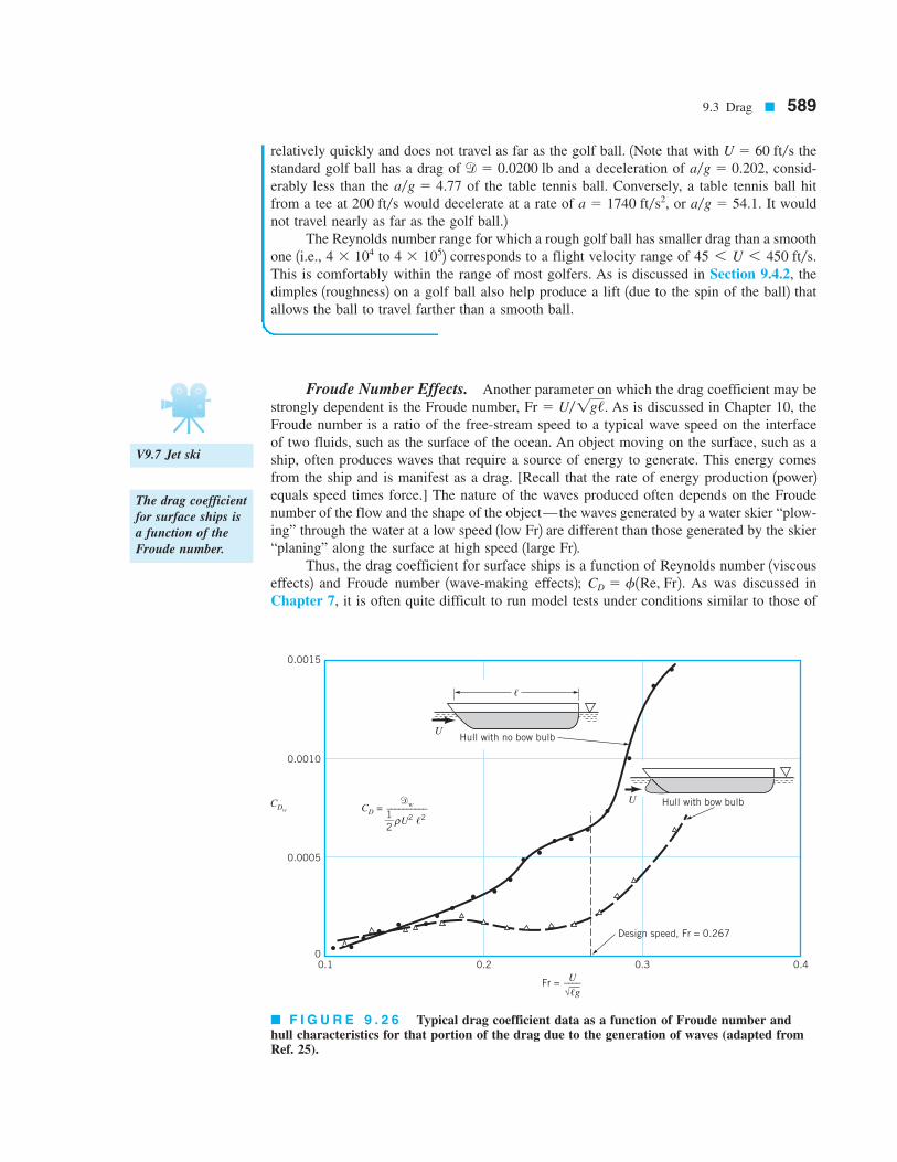
9.3 Drag ■ 589
relatively quickly and does not travel as far as the golf ball. 1Note that with the
standard golf ball has a drag of and a deceleration of consid-
erably less than the of the table tennis ball. Conversely, a table tennis ball hit
from a tee at would decelerate at a rate of or It would
not travel nearly as far as the golf ball.2The Reynolds number range for which a rough golf ball has smaller drag than a smooth
one 1i.e., to 2 corresponds to a flight velocity range of
This is comfortably within the range of most golfers. As is discussed in Section 9.4.2, the
dimples 1roughness2 on a golf ball also help produce a lift 1due to the spin of the ball2 that
allows the ball to travel farther than a smooth ball.
45 6 U 6 450 ft/s.4 3 1054 3 104
a/g 5 54.1.a 5 1740 ft/s2,200 ft/s
a/g 5 4.77
a/g 5 0.202,d 5 0.0200 lb
U 5 60 ft/s
Froude Number Effects. Another parameter on which the drag coefficient may be
strongly dependent is the Froude number, As is discussed in Chapter 10, the
Froude number is a ratio of the free-stream speed to a typical wave speed on the interface
of two fluids, such as the surface of the ocean. An object moving on the surface, such as a
ship, often produces waves that require a source of energy to generate. This energy comes
from the ship and is manifest as a drag. [Recall that the rate of energy production 1power2equals speed times force.] The nature of the waves produced often depends on the Froude
number of the flow and the shape of the object—the waves generated by a water skier “plow-
ing” through the water at a low speed 1low Fr2 are different than those generated by the skier
“planing” along the surface at high speed 1large Fr2.Thus, the drag coefficient for surface ships is a function of Reynolds number 1viscous
effects2 and Froude number 1wave-making effects2; As was discussed in
Chapter 7, it is often quite difficult to run model tests under conditions similar to those of
CD 5 f1Re, Fr2.
Fr 5 U/1g/.
■ F I G U R E 9 . 2 6 Typical drag coefficient data as a function of Froude number andhull characteristics for that portion of the drag due to the generation of waves (adapted fromRef. 25).
Design speed, Fr = 0.267
0.30.20.1
Hull with bow bulb
0.4
Hull with no bow bulb
U
U
,
0.0015
0.0010
0.0005
0
CD =CDw
$w__________
U2 ,21__2
ρ
Fr =U____
√,g
The drag coefficient
for surface ships is
a function of the
Froude number.
V9.7 Jet ski

the prototype 1i.e., same Re and Fr for surface ships2. Fortunately, the viscous and wave effects
can often be separated, with the total drag being the sum of the drag of these individual ef-
fects. A detailed account of this important topic can be found in standard texts 1Ref. 112.As is indicated in Fig. 9.26, the wave-making drag, can be a complex function of
the Froude number and the body shape. The rather “wiggly” dependence of wave drag co-
efficient, on the Froude number shown is typical. It results from the
fact that the structure of the waves produced by the hull is a strong function of the ship speed
or, in dimensionless form, the Froude number. This wave structure is also a function of the
body shape. For example, the bow wave, which is often the major contributor to the wave
drag, can be reduced by use of an appropriately designed bulb on the bow, as is indicated in
Fig. 9.26. In this instance the streamlined body 1hull without a bulb2 has more drag than the
less streamlined one.
Composite Body Drag. Approximate drag calculations for a complex body can of-
ten be obtained by treating the body as a composite collection of its various parts. For example,
the drag on an airplane can be approximated by adding the drag produced by its various com-
ponents—the wings, fuselage, tail section, and so on. Considerable care must be used in
such an approach because of the interactions between the various parts. For example, the
flow past the wing root 1near the wing-fuselage intersection2 is considerably altered by the
fuselage. Hence, it may not be correct to merely add the drag of the components to obtain
the drag of the entire object, although such approximations are often reasonable.
CDw 5 dw/ 1rU 2/
2/22,
dw,
590 ■ Chapter 9 / Flow Over Immersed Bodies
EXAMPLE
9.13
A 60-mph 1i.e., 88-fps2 wind blows past the water tower shown in Fig. E9.13a. Estimate the
moment 1torque2, M, needed at the base to keep the tower from tipping over.
SOLUTION
We treat the water tower as a sphere resting on a circular cylinder and assume that the total
drag is the sum of the drag from these parts. The free-body diagram of the tower is shown
in Fig. E.9.13b. By summing moments about the base of the tower, we obtain
(1)
where
(2)
and
(3)dc 51
2 rU 2bDcCDc
ds 51
2 rU 2
p
4 D2
sCDs
M 5 ds ab 1Ds
2b 1 dc ab
2b
The drag on a com-
plex body can be
approximated as
the sum of the drag
on its parts.
U = 60 mph =
88 fps
Ds = 40 ft
Dc = 15 ft
b = 50 ftb
Dc
Ds$s
$c
b + Ds /2
b/2
Rx
Ry
M
(b)(a)
0
■ F I G U R E E 9 . 1 3

9.3 Drag ■ 591
The aerodynamic drag on automobiles provides an example of the use of composite
bodies. The power required to move a car along a level street is used to overcome the rolling
resistance and the aerodynamic drag. For speeds above approximately 30 mph, the aerody-
namic drag becomes a significant contribution to the net propulsive force needed. The con-
tribution of the drag due to various portions of car 1i.e., front end, windshield, roof, rear end,
windshield peak, rear roofytrunk, and cowl2 have been determined by numerous model and
full-sized tests as well as by numerical calculations. As a result it is possible to predict the
aerodynamic drag on cars of a wide variety of body styles.
As is indicated in Fig. 9.27, the drag coefficient for cars has decreased rather contin-
uously over the years. This reduction is a result of careful design of the shape and the de-
tails 1such as window molding, rear view mirrors, etc.2. An additional reduction in drag has
been accomplished by a reduction of the projected area. The net result is a considerable in-
crease in the gas mileage, especially at highway speeds. Considerable additional information
about the aerodynamics of road vehicles can be found in the literature 1Ref. 302.
are the drag on the sphere and cylinder, respectively. For standard atmospheric conditions,
the Reynolds numbers are
and
The corresponding drag coefficients, and can be approximated from Fig. 9.21 as
Note that the value of was obtained by an extrapolation of the given data to Reynolds
numbers beyond those given 1a potentially dangerous practice!2. From Eqs. 2 and 3 we obtain
and
From Eq. 1 the corresponding moment needed to prevent the tower from tipping is
(Ans)
The above result is only an estimate because 1a2 the wind is probably not uniform from
the top of the tower to the ground, 1b2 the tower is not exactly a combination of a smooth
sphere and a circular cylinder, 1c2 the cylinder is not of infinite length, 1d2 there will be some
interaction between the flow past the cylinder and that past the sphere so that the net drag is
not exactly the sum of the two, and 1e2 a drag coefficient value was obtained by extrapola-
tion of the given data. However, such approximate results are often quite accurate.
M 5 3470 lb a50 ft 140
2 ftb 1 4840 lb a50
2 ftb 5 3.64 3 105 ft # lb
dc 5 0.512.38 3 1023 slugs/ft32 188 ft/s22150 ft 3 15 ft2 10.72 5 4840 lb
ds 5 0.512.38 3 1023 slugs/ft32 188 ft/s22 p
4 140 ft2210.32 5 3470 lb
CDs
CDs < 0.3 and CDc < 0.7
CDc,CDs
Rec 5UDc
n5188 ft/s2 115 ft2
1.57 3 1024 ft2/s
5 8.41 3 106
Res 5UDs
n5188 ft/s2 140 ft2
1.57 3 1024 ft2/s
5 2.24 3 107
Considerable effort
has gone into re-
ducing the aerody-
namic drag of auto-
mobiles.
V9.8 Drag on a
truck

The effect of several important parameters 1shape, Re, Ma, Fr, and roughness2 on the
drag coefficient for various objects has been discussed in this section. As stated previously,
drag coefficient information for a very wide range of objects is available in the literature.
Some of this information is given in Figs. 9.28, 9.29, and 9.30 for a variety of two- and three-
dimensional, natural and manmade objects. Recall that a drag coefficient of unity is equiva-
lent to the drag produced by the dynamic pressure acting on an area of size A. That is,
if Typical nonstreamlined objects have drag coefficients
on this order.
CD 5 1.d 512rU
2ACD 512rU
2A
592 ■ Chapter 9 / Flow Over Immersed Bodies
9.4 Lift
As is indicated in Section 9.1, any object moving through a fluid will experience a net force
of the fluid on the object. For symmetrical objects, this force will be in the direction of the
free stream—a drag, If the object is not symmetrical 1or if it does not produce a sym-
metrical flow field, such as the flow around a rotating sphere2, there may also be a force nor-
mal to the free stream—a lift, Considerable effort has been put forth to understand the
various properties of the generation of lift. Some objects, such as an airfoil, are designed to
generate lift. Other objects are designed to reduce the lift generated. For example, the lift on
a car tends to reduce the contact force between the wheels and the ground, causing reduc-
tion in traction and cornering ability. It is desirable to reduce this lift.
9.4.1 Surface Pressure Distribution
The lift can be determined from Eq. 9.2 if the distributions of pressure and wall shear stress
around the entire body are known. As is indicated in Section 9.1, such data are usually not
known. Typically, the lift is given in terms of the lift coefficient.
(9.39)
which is obtained from experiments, advanced analysis, or numerical considerations. The
lift coefficient is a function of the appropriate dimensionless parameters and, as the drag
CL 5
l
12rU
2A
l.
d.
The lift coefficient
is a dimensionless
form of the lift.
0.8
0.6
0.4
0.2
01920 1930 1940 1950 1960
Year
1970 1980 1990 2000
CD
■ F I G U R E 9 . 2 7 The historical trend of streamlining automobiles to reduce their aero-dynamic drag and increase their miles per gallon (adapted from Ref. 5).

coefficient, can be written as
The Froude number, Fr, is important only if there is a free surface present, as with an un-
derwater “wing” used to support a high-speed hydrofoil surface ship. Often the surface rough-
ness, is relatively unimportant in terms of lift—it has more of an effect on the drag. The
Mach number, Ma, is of importance for relatively high-speed subsonic and supersonic flows
and the Reynolds number effect is often not great. The most important pa-
rameter that affects the lift coefficient is the shape of the object. Considerable effort has gone
into designing optimally shaped lift-producing devices. We will emphasize the effect of the
1i.e., Ma 7 0.82,
e,
CL 5 f1shape, Re, Ma, Fr, e//2
9.4 Lift ■ 593
The lift coefficient
is a function of
other dimensionless
parameters.
■ F I G U R E 9 . 2 8 Typical drag coefficients for regular two-dimensional objects (Refs. 5and 6).
D
R
Square rod
with rounded
corners
DR
Rounded
equilateral
triangle
DSemicircular
shell
Semicircular
cylinderD
D T-beam
I-beamD
D Angle
D
Hexagon
,
D Rectangle
ShapeReference area
A(b = length)
A = bD
A = bD
A = bD
A = bD
A = bD
A = bD
A = bD
A = bD
A = bD
Drag coefficient
CD =$________
U2A1__2
ρ
R/D CD
00.02
0.170.33
2.22.0
1.21.0
R/D CD
00.020.080.25
1.41.21.31.1
2.12.01.91.3
2.3
1.1
2.15
1.15
1.80
1.65
1.98
1.82
2.05
1.0
,/D CD
0.1
0.5
0.65
1.0
2.0
3.0
1.9
2.5
2.9
2.2
1.6
1.3
Reynolds number
Re = UD/ ρ
Re = 105
Re = 105
Re = 2 × 10⁴
Re > 104
Re > 104
Re > 104
Re > 104
Re > 104
Re = 105
<
µ

shape on lift—the effects of the other dimensionless parameters can be found in the litera-
ture 1Refs. 13, 14, 292.Most common lift-generating devices 1i.e., airfoils, fans, spoilers on cars, etc.2 operate
in the large Reynolds number range in which the flow has a boundary layer character, with
viscous effects confined to the boundary layers and wake regions. For such cases the wall
shear stress, contributes little to the lift. Most of the lift comes from the surface pressure
distribution. A typical pressure distribution on a moving car is shown in Fig. 9.31. The dis-
tribution, for the most part, is consistent with simple Bernoulli equation analysis. Locations
with high-speed flow 1i.e., over the roof and hood2 have low pressure, while locations with
low-speed flow 1i.e., on the grill and windshield2 have high pressure. It is easy to believe that
the integrated effect of this pressure distribution would provide a net upward force.
tw,
594 ■ Chapter 9 / Flow Over Immersed Bodies
Usually most lift
comes from pres-
sure forces, not vis-
cous forces.
■ F I G U R E 9 . 2 9 Typical drag coefficients for regular three-dimensional objects (Ref. 5).
DSolid
hemisphere
DHollow
hemisphere
D Thin disk
,
D
Circular
rod
parallel
to flow
D Cone
CubeD
Cube
D
D
Streamlined
body
ShapeReference area
A
A = D2__4π
A = D2__4π
A = D2__4π
A = D2__4π
A = D2__4π
A = D2
A = D2
A = D2__4π
Drag coefficient
CD
1.17
0.42
1.42
0.38
1.1
, degrees CD
10
30
60
90
0.30
0.55
0.80
1.15
,/D CD
0.5
1.0
2.0
4.0
1.1
0.93
0.83
0.85
θ
1.05
0.80
0.04
Re > 104
Re > 104
Re > 103
Re > 105
Re > 104
Re > 104
Re > 104
Re > 105
Reynolds number
Re = UD/ ρ µ
θ

9.4 Lift ■ 595
■ F I G U R E 9 . 3 0 Typical drag coefficients for objects of interest (Refs. 5, 6, 15, and 20).
U
D Parachute
D Porous
parabolic
dish
Average
person
Fluttering
flagD
l
Empire
State Building
Six-car passenger train
Bikes
Upright commuter
Racing
Drafting
Streamlined
Tractor-trailor tucks
Fairing
Gap seal
Standard
With fairing
With
fairing and
gap seal
TreeU = 10 m/s
U = 20 m/s
U = 30 m/s
Dolphin
Large
birds
Shape Reference area
Frontal area
A = D2__4π
Frontal area
A = D2__4π
Standing
Sitting
Crouching
A = ,D
Frontal area
Frontal area
A = 5.5 ft2
A = 3.9 ft2
A = 3.9 ft2
A = 5.0 ft2
Frontal area
Frontal area
Frontal area
Frontal area
Frontal area
Wetted area
Drag coefficient
CD
1.4
Porosity
Porosity = open area/total area
0 0.2 0.5
1.42 1.20 0.82
0.95 0.90 0.80
CDA = 9 ft2
CDA = 6 ft2
CDA = 2.5 ft2
,/D CD
21
3
0.120.07
0.15
1.4
1.8
1.1
0.88
0.50
0.12
0.96
0.76
0.70
0.43
0.26
0.20
0.0036 at Re = 6 × 10⁶
(flat plate has CDf = 0.0031)
0.40

596 ■ Chapter 9 / Flow Over Immersed Bodies
EXAMPLE
9.14
U, p0
Denotes p > p0
Denotes p < p0
For objects operating in very low Reynolds number regimes viscous
effects are important, and the contribution of the shear stress to the lift may be as important
as that of the pressure. Such situations include the flight of minute insects and the swimming
of microscopic organisms. The relative importance of and p in the generation of lift in a
typical large Reynolds number flow is shown in Example 9.14.
tw
1i.e., Re 6 12,
■ F I G U R E 9 . 3 1 Pressure distribution on the surface of an automobile.
The relative impor-
tance of shear
stress and pressure
effects depends
strongly on the
Reynolds number.
When a uniform wind of velocity U blows past the semicircular building shown in Fig. E9.14a,
the wall shear stress and pressure distributions on the outside of the building are as given
previously in Figs. E9.8b and E9.9a, respectively. If the pressure in the building is atmos-
pheric 1i.e., the value, far from the building2, determine the lift coefficient and the lift on
the roof.
SOLUTION
From Eq. 9.2 we obtain the lift as
(1)
As is indicated in Fig. E9.14a, we assume that on the inside of the building the pressure is
uniform, and that there is no shear stress. Thus, Eq. 1 can be written as
or
(2)
where b and D are the length and diameter of the building, respectively, and
Equation 2 can be put into dimensionless form by using the dynamic pressure, plan-
form area, and dimensionless shear stress
to give
(3)
The values of the two integrals in Eq. 3 can be obtained by determining the area under the
curves of and plotted in Figs. E9.14bF1u2 cos u versus u3 1p 2 p02/ 1rU 2/22 4 sin u versus u
l 51
2 rU 2A c21
2 #p
0
1p 2 p02
12rU
2 sin u du 1
1
21Re #p
0
F1u2 cos u du d
F1u2 5 tw1Re21/2/ 1rU 2
/22A 5 bD,
rU 2/2,
dA 5 b1D/22du.l 5
bD
2 c2#
p
0
1p 2 p02 sin u du 1 #p
0
tw cos u du d
l 5 2#p
0
1p 2 p02 sin u b aD
2b du 1 #
p
0
tw cos u b aD
2b du
p 5 p0,
l 5 2# p sin u dA 1 # tw cos u dA
p0,

9.4 Lift ■ 597
and E9.14c. The results are
and
Thus, the lift is
or
(Ans)
and
(4) (Ans)CL 5l
1
2rU2A
5 0.88 11.96
1Re
l 5 a0.88 11.96
1Reb a1
2 rU 2Ab
l 51
2 rU 2A c a21
2b 121.762 1
1
21Re 13.922 d
#p
0
F1u2 cos u du 5 3.92
#p
0
1p 2 p02
1
2rU2
sin u du 5 21.76
d
w dA
p0 dA
pdA
D/2
θ
τ
θ
U
p0
(a)
(b) (c)
1.0
0.5
0
–0.5
–1.0
–1.50
Cp s
in =
θp –
p0
____
___
U
21 __ 2
ρ
π __
4
π __
2
3 ___
4
π 00
2
4
6
π __
4
π __
2
π3 ___
4
π
θ, rad θ, rad
F(
) c
os
θ
θ
π
■ F I G U R E E 9 . 1 4
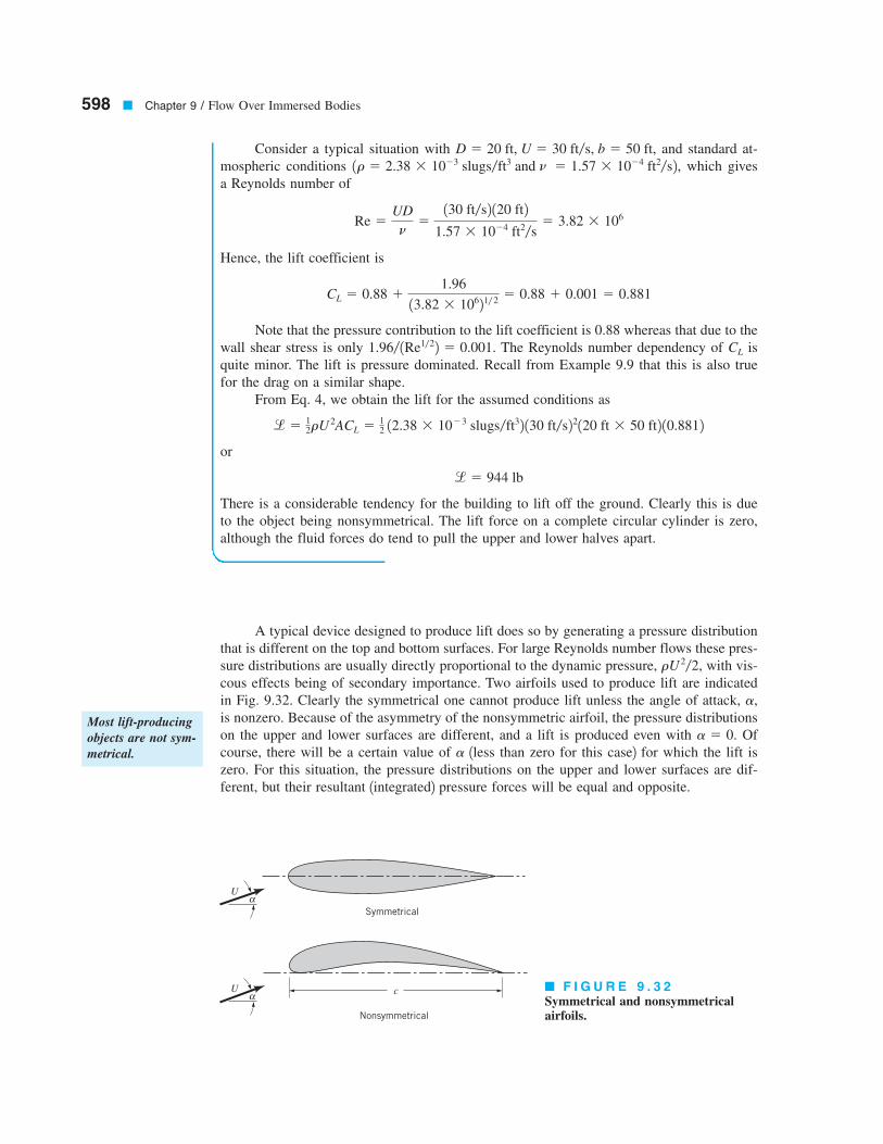
598 ■ Chapter 9 / Flow Over Immersed Bodies
Consider a typical situation with and standard at-
mospheric conditions which gives
a Reynolds number of
Hence, the lift coefficient is
Note that the pressure contribution to the lift coefficient is 0.88 whereas that due to the
wall shear stress is only The Reynolds number dependency of is
quite minor. The lift is pressure dominated. Recall from Example 9.9 that this is also true
for the drag on a similar shape.
From Eq. 4, we obtain the lift for the assumed conditions as
or
There is a considerable tendency for the building to lift off the ground. Clearly this is due
to the object being nonsymmetrical. The lift force on a complete circular cylinder is zero,
although the fluid forces do tend to pull the upper and lower halves apart.
l 5 944 lb
l 512rU
2ACL 512 12.38 3 1023 slugs/ft
32 130 ft/s22120 ft 3 50 ft2 10.8812
CL1.96/ 1Re1/22 5 0.001.
CL 5 0.88 11.96
13.82 3 10621/ 25 0.88 1 0.001 5 0.881
Re 5UD
n5130 ft/s2 120 ft2
1.57 3 1024 ft2/s
5 3.82 3 106
1r 5 2.38 3 1023 slugs/ft3 and n 5 1.57 3 1024 ft2
/s2,D 5 20 ft, U 5 30 ft/s, b 5 50 ft,
A typical device designed to produce lift does so by generating a pressure distribution
that is different on the top and bottom surfaces. For large Reynolds number flows these pres-
sure distributions are usually directly proportional to the dynamic pressure, with vis-
cous effects being of secondary importance. Two airfoils used to produce lift are indicated
in Fig. 9.32. Clearly the symmetrical one cannot produce lift unless the angle of attack,
is nonzero. Because of the asymmetry of the nonsymmetric airfoil, the pressure distributions
on the upper and lower surfaces are different, and a lift is produced even with Of
course, there will be a certain value of 1less than zero for this case2 for which the lift is
zero. For this situation, the pressure distributions on the upper and lower surfaces are dif-
ferent, but their resultant 1integrated2 pressure forces will be equal and opposite.
a
a 5 0.
a,
rU 2/2,
■ F I G U R E 9 . 3 2
Symmetrical and nonsymmetricalairfoils.
α
U
Symmetrical
Nonsymmetrical
c
α
U
Most lift-producing
objects are not sym-
metrical.

Since most airfoils are thin, it is customary to use the planform area, in the
definition of the lift coefficient. Here b is the length of the airfoil and c is the chord length—
the length from the leading edge to the trailing edge as indicated in Fig. 9.32. Typical lift
coefficients so defined are on the order of unity. That is, the lift force is on the order of the
dynamic pressure times the planform area of the wing, The wing loading,
defined as the average lift per unit area of the wing, therefore, increases with speed.
For example, the wing loading of the 1903 Wright Flyer aircraft was while for the
present-day Boeing 747 aircraft it is The wing loading for a bumble bee is ap-
proximately 1Ref. 152.Typical lift and drag coefficient data as a function of angle of attack, and aspect ra-
tio, are indicated in Figs. 9.33a and 9.33b. The aspect ratio is defined as the ratio of the
square of the wing length to the planform area, If the chord length, c, is constant
along the length of the wing 1a rectangular planform wing2, this reduces to
In general, the lift coefficient increases and the drag coefficient decreases with an in-
crease in aspect ratio. Long wings are more efficient because their wing tip losses are
a 5 b/c.
a 5 b2/A.
a,
a,
1 lb/ft2
150 lb/ft2.
1.5 lb/ft2,
l/A,
l < 1rU 2/22A.
9.4 Lift ■ 599
■ F I G U R E 9 . 3 3 Typical lift and drag coefficient data as a func-tion of angle of attack and the aspect ratio of the airfoil: (a) lift coefficient,(b) drag coefficient.
–0.4 –10 0 10
, degrees
(a)
(b)
α
, degreesα
20
–0.2
0
0.2
0.4
0.6
0.8
1.0
1.2
1.4
CL
CD
! = 7
! = 3
! = 1
! = 1 ! = 3
! = 7
0.03
0.02
0.01
0–10 0 10 20
Lift and drag coef-
ficients for wings
are functions of the
angle of attack.
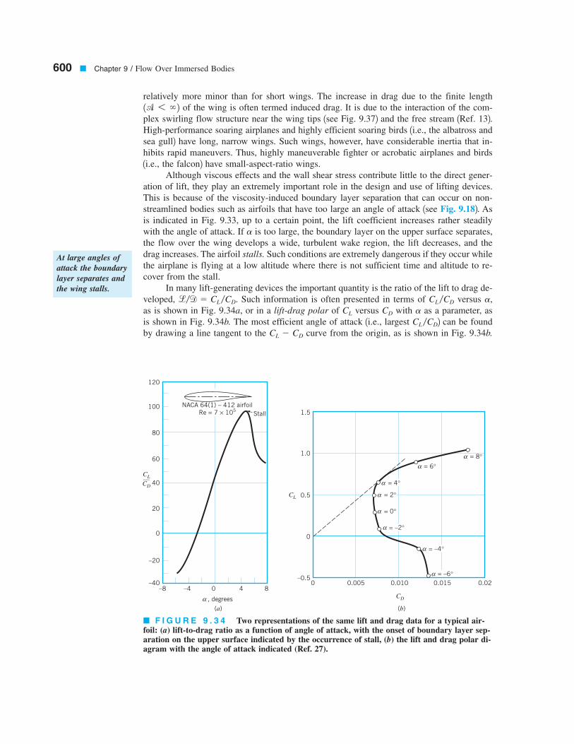
relatively more minor than for short wings. The increase in drag due to the finite length
of the wing is often termed induced drag. It is due to the interaction of the com-
plex swirling flow structure near the wing tips 1see Fig. 9.372 and the free stream 1Ref. 132.High-performance soaring airplanes and highly efficient soaring birds 1i.e., the albatross and
sea gull2 have long, narrow wings. Such wings, however, have considerable inertia that in-
hibits rapid maneuvers. Thus, highly maneuverable fighter or acrobatic airplanes and birds
1i.e., the falcon2 have small-aspect-ratio wings.
Although viscous effects and the wall shear stress contribute little to the direct gener-
ation of lift, they play an extremely important role in the design and use of lifting devices.
This is because of the viscosity-induced boundary layer separation that can occur on non-
streamlined bodies such as airfoils that have too large an angle of attack 1see Fig. 9.182. As
is indicated in Fig. 9.33, up to a certain point, the lift coefficient increases rather steadily
with the angle of attack. If is too large, the boundary layer on the upper surface separates,
the flow over the wing develops a wide, turbulent wake region, the lift decreases, and the
drag increases. The airfoil stalls. Such conditions are extremely dangerous if they occur while
the airplane is flying at a low altitude where there is not sufficient time and altitude to re-
cover from the stall.
In many lift-generating devices the important quantity is the ratio of the lift to drag de-
veloped, Such information is often presented in terms of versus
as is shown in Fig. 9.34a, or in a lift-drag polar of versus with as a parameter, as
is shown in Fig. 9.34b. The most efficient angle of attack 1i.e., largest 2 can be found
by drawing a line tangent to the curve from the origin, as is shown in Fig. 9.34b.CL 2 CD
CL /CD
aCDCL
a,CL /CDl/d 5 CL /CD.
a
1a 6 ` 2
600 ■ Chapter 9 / Flow Over Immersed Bodies
At large angles of
attack the boundary
layer separates and
the wing stalls.
■ F I G U R E 9 . 3 4 Two representations of the same lift and drag data for a typical air-foil: (a) lift-to-drag ratio as a function of angle of attack, with the onset of boundary layer sep-aration on the upper surface indicated by the occurrence of stall, (b) the lift and drag polar di-agram with the angle of attack indicated (Ref. 27).
120
100
80
60
40
20
0
–20
–40–8 –4 0 4 8
, degreesα
CL__CD
NACA 64(1) – 412 airfoil
Re = 7 × 10⁵Stall 1.5
1.0
0.5
0
–0.50 0.005 0.010 0.015 0.02
CD
CL
(b)(a)
= –6°α
= –4°α
= –2°α
= 0°α
= 2°α
= 4°α
= 6°α
= 8°α

High-performance airfoils generate lift that is perhaps 100 or more times greater than their
drag. This translates into the fact that in still air they can glide a horizontal distance of 100 m
for each 1 m drop in altitude.
As is indicated above, the lift and drag on an airfoil can be altered by changing the an-
gle of attack. This actually represents a change in the shape of the object. Other shape changes
can be used to alter the lift and drag when desirable. In modern airplanes it is common to
utilize leading edge and trailing edge flaps as is shown in Fig. 9.35. To generate the neces-
sary lift during the relatively low-speed landing and takeoff procedures, the airfoil shape is
altered by extending special flaps on the front andyor rear portions of the wing. Use of the
flaps considerably enhances the lift, although it is at the expense of an increase in the drag
1the airfoil is in a “dirty” configuration2. This increase in drag is not of much concern dur-
ing landing and takeoff operations—the decrease in landing or takeoff speed is more im-
portant than is a temporary increase in drag. During normal flight with the flaps retracted
1the “clean” configuration2, the drag is relatively small, and the needed lift force is achieved
with the smaller lift coefficient and the larger dynamic pressure 1higher speed2.The use of the complex flap systems for modern aircraft has proved to be an impor-
tant breakthrough in aeronautics. Actually, certain birds use the leading edge flap concept.
Some species have special feathers on the leading edge of their wings that extend as a lead-
ing edge flap when low-speed flight is required 1such as when their wings are fully extended
during landing2 1Ref. 152.A wide variety of lift and drag information for airfoils can be found in standard aero-
dynamics books 1Ref. 13, 14, 292.
9.4 Lift ■ 601
Flaps alter the lift
and drag character-
istics of a wing.
No flaps
Trailing edge
slotted flap
Double slotted
trailing edge flaps
(Data not
shown)
Leading
edge flap
3.0
2.0
1.0
00 0.1 0.2 0.3
CD
CL
■ F I G U R E 9 . 3 5
Typical lift and drag alter-ations possible with the useof various types of flap de-signs (Ref. 21).
602 ■ Chapter 9 / Flow Over Immersed Bodies
EXAMPLE
9.15
In 1977 the Gossamer Condor won the Kremer prize by being the first human-powered air-
craft to complete a prescribed figure-of-eight course around two turning points 0.5 mi apart1Ref. 222. The following data pertain to this aircraft:
Determine the lift coefficient, and the power, required by the pilot.
SOLUTION
For steady flight conditions the lift must be exactly balanced by the weight, or
Thus,
where and for
standard air. This gives
(Ans)
a reasonable number. The overall-lift-to drag ratio for the aircraft is
23.7.The product of the power that the pilot supplies and the power train efficiency equals
the useful power needed to overcome the drag, That is,
where
Thus,
(1)
or
(Ans) p 5 166 ft # lb/s a 1 hp
550 ft # lb/sb 5 0.302 hp
p 512.38 3 1023 slugs/ft
32 1720 ft22 10.0462 115 ft/s23210.82
p 5dU
h5
12rU
2ACDU
h5rACDU 3
2h
d 512rU
2ACD
hp 5 dU
d.
CL /CD 5 1.09/0.046 5
CL 521210 lb2
12.38 3 1023 slugs/ft32 115 ft/s221720 ft22 5 1.09
r 5 2.38 3 1023 slugs/ft3A 5 bc 5 96 ft 3 7.5 ft 5 720 ft2, w 5 210 lb,
CL 52w
rU 2A
w 5 l 512rU
2ACL
p,CL,
power train efficiency 5 h 5 power to overcome drag/pilot power 5 0.8
drag coefficient 5 CD 5 0.046 1based on planform area2 weight 1including pilot2 5w 5 210 lb
wing size 5 b 5 96 ft, c 5 7.5 ft 1average2 flight speed 5 U 5 15 ft/s

9.4.2 Circulation
Since viscous effects are of minor importance in the generation of lift, it should be possible
to calculate the lift force on an airfoil by integrating the pressure distribution obtained from
the equations governing inviscid flow past the airfoil. That is, the potential flow theory dis-
cussed in Chapter 6 should provide a method to determine the lift. Although the details are
beyond the scope of this book, the following is found from such calculations 1Ref. 42.The calculation of the inviscid flow past a two-dimensional airfoil gives a flow field
as indicated in Fig. 9.36. The predicted flow field past an airfoil with no lift 1i.e., a sym-
metrical airfoil at zero angle of attack, Fig. 9.36a2 appears to be quite accurate 1except for
the absence of thin boundary layer regions2. However, as is indicated in Fig. 9.36b, the
9.4 Lift ■ 603
This power level is obtainable by a well-conditioned athlete 1as is indicated by the fact that
the flight was successfully completed2. Note that only 80% of the pilot’s power 1i.e.,
which corresponds to a drag of 2 is needed to force the
aircraft through the air. The other 20% is lost because of the power train inefficiency. Note
from Eq. 1 that for a constant drag coefficient the power required increases as —a dou-
bling of the speed to would require an eightfold increase in power 1i.e., 2.42 hp, well
beyond the range of any human2.30 ft/s
U3
d 5 8.86 lb0.8 3 0.302 5 0.242 hp,
Inviscid flow analy-
sis can be used to
obtain ideal flow
past airfoils.
(a)
(b)
(c)
+ =
(d)
= 0
+ = 0
α
> 0
+ = 0
α
> 0
+ > 0
α
"(a) + circulation = (c)"
■ F I G U R E 9 . 3 6
Inviscid flow past anairfoil: (a) symmetri-cal flow past the sym-metrical airfoil at azero angle of attacks;(b) same airfoil at anonzero angle of at-tack—no lift, flownear trailing edge notrealistic; (c) same con-ditions as for (b) ex-cept circulation hasbeen added to theflow—nonzero lift, re-alistic flow; (d) super-position of flows toproduce the final flowpast the airfoil.
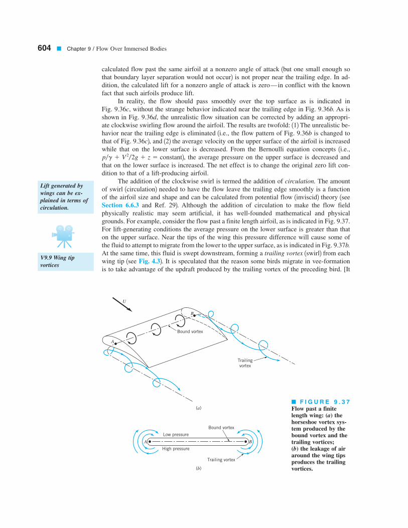
calculated flow past the same airfoil at a nonzero angle of attack 1but one small enough so
that boundary layer separation would not occur2 is not proper near the trailing edge. In ad-
dition, the calculated lift for a nonzero angle of attack is zero—in conflict with the known
fact that such airfoils produce lift.
In reality, the flow should pass smoothly over the top surface as is indicated in
Fig. 9.36c, without the strange behavior indicated near the trailing edge in Fig. 9.36b. As is
shown in Fig. 9.36d, the unrealistic flow situation can be corrected by adding an appropri-
ate clockwise swirling flow around the airfoil. The results are twofold: 112 The unrealistic be-
havior near the trailing edge is eliminated 1i.e., the flow pattern of Fig. 9.36b is changed to
that of Fig. 9.36c2, and 122 the average velocity on the upper surface of the airfoil is increased
while that on the lower surface is decreased. From the Bernoulli equation concepts 1i.e.,
2, the average pressure on the upper surface is decreased and
that on the lower surface is increased. The net effect is to change the original zero lift con-
dition to that of a lift-producing airfoil.
The addition of the clockwise swirl is termed the addition of circulation. The amount
of swirl 1circulation2 needed to have the flow leave the trailing edge smoothly is a function
of the airfoil size and shape and can be calculated from potential flow 1inviscid2 theory 1see
Section 6.6.3 and Ref. 292. Although the addition of circulation to make the flow field
physically realistic may seem artificial, it has well-founded mathematical and physical
grounds. For example, consider the flow past a finite length airfoil, as is indicated in Fig. 9.37.
For lift-generating conditions the average pressure on the lower surface is greater than that
on the upper surface. Near the tips of the wing this pressure difference will cause some of
the fluid to attempt to migrate from the lower to the upper surface, as is indicated in Fig. 9.37b.
At the same time, this fluid is swept downstream, forming a trailing vortex 1swirl2 from each
wing tip 1see Fig. 4.32. It is speculated that the reason some birds migrate in vee-formation
is to take advantage of the updraft produced by the trailing vortex of the preceding bird. [It
p/g 1 V 2/2g 1 z 5 constant
604 ■ Chapter 9 / Flow Over Immersed Bodies
Lift generated by
wings can be ex-
plained in terms of
circulation.
V9.9 Wing tip
vortices
■ F I G U R E 9 . 3 7
Flow past a finite length wing: (a) thehorseshoe vortex sys-tem produced by thebound vortex and thetrailing vortices; (b) the leakage of airaround the wing tipsproduces the trailingvortices.
U
A
B
Bound vortex
Trailing
vortex
(a)
(b)
BA
Low pressure
High pressure
Bound vortex
Trailing vortex
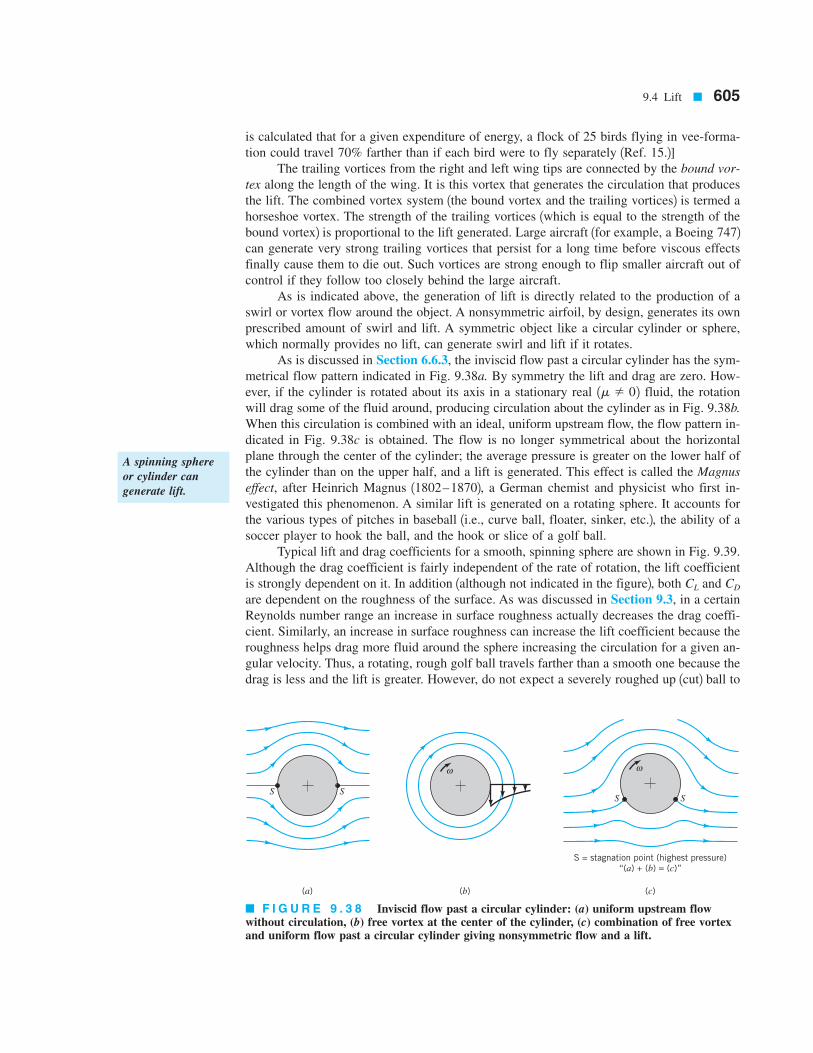
is calculated that for a given expenditure of energy, a flock of 25 birds flying in vee-forma-
tion could travel 70% farther than if each bird were to fly separately 1Ref. 15.2]The trailing vortices from the right and left wing tips are connected by the bound vor-
tex along the length of the wing. It is this vortex that generates the circulation that produces
the lift. The combined vortex system 1the bound vortex and the trailing vortices2 is termed a
horseshoe vortex. The strength of the trailing vortices 1which is equal to the strength of the
bound vortex2 is proportional to the lift generated. Large aircraft 1for example, a Boeing 7472can generate very strong trailing vortices that persist for a long time before viscous effects
finally cause them to die out. Such vortices are strong enough to flip smaller aircraft out of
control if they follow too closely behind the large aircraft.
As is indicated above, the generation of lift is directly related to the production of a
swirl or vortex flow around the object. A nonsymmetric airfoil, by design, generates its own
prescribed amount of swirl and lift. A symmetric object like a circular cylinder or sphere,
which normally provides no lift, can generate swirl and lift if it rotates.
As is discussed in Section 6.6.3, the inviscid flow past a circular cylinder has the sym-
metrical flow pattern indicated in Fig. 9.38a. By symmetry the lift and drag are zero. How-
ever, if the cylinder is rotated about its axis in a stationary real fluid, the rotation
will drag some of the fluid around, producing circulation about the cylinder as in Fig. 9.38b.
When this circulation is combined with an ideal, uniform upstream flow, the flow pattern in-
dicated in Fig. 9.38c is obtained. The flow is no longer symmetrical about the horizontal
plane through the center of the cylinder; the average pressure is greater on the lower half of
the cylinder than on the upper half, and a lift is generated. This effect is called the Magnus
effect, after Heinrich Magnus 11802–18702, a German chemist and physicist who first in-
vestigated this phenomenon. A similar lift is generated on a rotating sphere. It accounts for
the various types of pitches in baseball 1i.e., curve ball, floater, sinker, etc.2, the ability of a
soccer player to hook the ball, and the hook or slice of a golf ball.
Typical lift and drag coefficients for a smooth, spinning sphere are shown in Fig. 9.39.
Although the drag coefficient is fairly independent of the rate of rotation, the lift coefficient
is strongly dependent on it. In addition 1although not indicated in the figure2, both and
are dependent on the roughness of the surface. As was discussed in Section 9.3, in a certain
Reynolds number range an increase in surface roughness actually decreases the drag coeffi-
cient. Similarly, an increase in surface roughness can increase the lift coefficient because the
roughness helps drag more fluid around the sphere increasing the circulation for a given an-
gular velocity. Thus, a rotating, rough golf ball travels farther than a smooth one because the
drag is less and the lift is greater. However, do not expect a severely roughed up 1cut2 ball to
CDCL
1m Þ 02
9.4 Lift ■ 605
A spinning sphere
or cylinder can
generate lift.
■ F I G U R E 9 . 3 8 Inviscid flow past a circular cylinder: (a) uniform upstream flowwithout circulation, (b) free vortex at the center of the cylinder, (c) combination of free vortexand uniform flow past a circular cylinder giving nonsymmetric flow and a lift.
S S
ωω
S S
S = stagnation point (highest pressure)
“(a) + (b) = (c)”
(c)(b)(a)
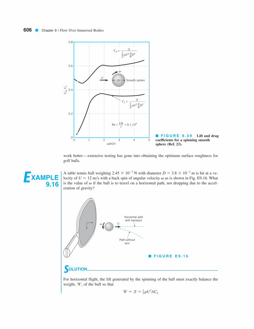
work better—extensive testing has gone into obtaining the optimum surface roughness for
golf balls.
606 ■ Chapter 9 / Flow Over Immersed Bodies
EXAMPLE
9.16
A table tennis ball weighing with diameter is hit at a ve-
locity of with a back spin of angular velocity as is shown in Fig. E9.16. What
is the value of if the ball is to travel on a horizontal path, not dropping due to the accel-
eration of gravity?
v
vU 5 12 m/s
D 5 3.8 3 1022 m2.45 3 1022 N
■ F I G U R E 9 . 3 9 Lift and dragcoefficients for a spinning smoothsphere (Ref. 23).
■ F I G U R E E 9 . 1 6
Smooth sphereDU
ω
00
0.2
0.4
0.6
0.8
1 2 3
D/2Uω
4 5
Re = = 6 × 10⁴UD___v
CL =+ ____________
U2
D21__
2 __4
ρπ
CD =$ ____________
U2
D21__
2 __4
ρπ
CD,
CL
SOLUTION
For horizontal flight, the lift generated by the spinning of the ball must exactly balance the
weight, of the ball so that
w 5 l 512rU
2ACL
w,
ω U
Horizontal path
with backspin
Path without
spin

References ■ 607
or
where the lift coefficient, can be obtained from Fig. 9.39. For standard atmospheric con-
ditions with we obtain
which, according to Fig. 9.39, can be achieved if
or
Thus,
(Ans)
Is it possible to impart this angular velocity to the ball? With larger angular velocities
the ball will rise and follow an upward curved path. Similar trajectories can be produced by
a well-hit golf ball—rather than falling like a rock, the golf ball trajectory is actually curved
up and the spinning ball travels a greater distance than one without spin. However, if top
spin is imparted to the ball 1as in an improper tee shot2 the ball will curve downward more
quickly than under the action of gravity alone—the ball is “topped” and a negative lift is
generated. Similarly, rotation about a vertical axis will cause the ball to hook or slice to one
side or the other.
v 5 1568 rad/s2 160 s/min2 11 rev/2p rad2 5 5420 rpm
v 52U10.92
D5
2112 m/s2 10.92
3.8 3 1022 m5 568 rad/s
vD
2U5 0.9
CL 5212.45 3 1022 N2
11.23 kg/m32 112 m/s2
21p/42 13.8 3 1022 m225 0.244
r 5 1.23 kg/m3
CL,
CL 52w
rU 21p/42D2
Key Words and Topics
In the E-book, click on any key word
or topic to go to that subject.
Adverse pressure gradient
Blasius solution
Boundary layer
Boundary layer separation
Boundary layer thickness
Boundary layer transition
Circulation
Drag
Drag coefficient
Favorable pressure gradient
Flow separation
Form drag
Free-stream velocity
Friction drag
Laminar boundary layer
Lift
Lift coefficient
Momentum–integral equation
Pressure coefficient
Pressure drag
Stall
Turbulent boundary layer
Upstream velocity
Wake
References
1. Schlichting, H., Boundary Layer Theory, 7th Ed., McGraw-Hill, New York, 1979.
2. Rosenhead, L., Laminar Boundary Layers, Oxford Univer-sity Press, London, 1963.
3. White, F. M., Viscous Fluid Flow, McGraw-Hill, New York,1974.
4. Currie, I. G., Fundamental Mechanics of Fluids, McGraw-Hill, New York, 1974.

5. Blevins, R. D., Applied Fluid Dynamics Handbook, Van Nos-trand Reinhold, New York, 1984.
6. Hoerner, S. F., Fluid-Dynamic Drag, published by the au-thor, Library of Congress No. 64,19666, 1965.
7. Happel, J., Low Reynolds Number Hydrodynamics, PrenticeHall, Englewood Cliffs, NJ, 1965.
8. Van Dyke, M., An Album of Fluid Motion, Parabolic Press,Stanford, Calif., 1982.
9. Thompson, P. A., Compressible-Fluid Dynamics, McGraw-Hill, New York, 1972.
10. Zucrow, M. J., and Hoffman, J. D., Gas Dynamics, Vol. I,Wiley, New York, 1976.
11. Clayton, B. R., and Bishop, R. E. D., Mechanics of MarineVehicles, Gulf Publishing Co., Houston, 1982.
12. CRC Handbook of Tables for Applied Engineering Science,2nd Ed., CRC Press, 1973.
13. Shevell, R. S., Fundamentals of Flight, 2nd Ed., PrenticeHall, Englewood Cliffs, NJ, 1989.
14. Kuethe, A. M. and Chow, C. Y., Foundations of Aerody-namics, Bases of Aerodynamics Design, 4th Ed., Wiley, 1986.
15. Vogel, J., Life in Moving Fluids, 2nd Ed., Willard GrantPress, Boston, 1994.
16. Kreider, J. F., Principles of Fluid Mechanics, Allyn and Ba-con, Newton, Mass., 1985.
17. Dobrodzicki, G. A., Flow Visualization in the NationalAeronautical Establishment’s Water Tunnel, National Re-search Council of Canada, Aeronautical Report LR-557,1972.
18. White, F. M., Fluid Mechanics, McGraw-Hill, New York,1986.
19. Vennard, J. K., and Street, R. L., Elementary Fluid Me-chanics, 6th Ed., Wiley, New York, 1982.
20. Gross, A. C., Kyle, C. R., and Malewicki, D. J., The Aero-dynamics of Human Powered Land Vehicles, Scientific Ameri-can, Vol. 249, No. 6, 1983.
21. Abbott, I. H., and Von Doenhoff, A. E., Theory of WingSections, Dover Publications, New York, 1959.
22. MacReady, P. B., “Flight on 0.33 Horsepower: The Gos-samer Condor,” Proc. AIAA 14th Annual Meeting 1Paper No.78-3082, Washington, DC, 1978.
23. Goldstein, S., Modern Developments in Fluid Dynamics,Oxford Press, London, 1938.
24. Achenbach, E., Distribution of Local Pressure and SkinFriction around a Circular Cylinder in Cross-Flow up to
Journal of Fluid Mechanics, Vol. 34, Pt. 4,1968.
25. Inui, T., Wave-Making Resistance of Ships, Transactionsof the Society of Naval Architects and Marine Engineers, Vol.70, 1962.
26. Sovran, G., et al. 1ed.2, Aerodynamic Drag Mechanisms ofBluff Bodies and Road Vehicles, Plenum Press, New York,1978.
27. Abbott, I. H., von Doenhoff, A. E. and Stivers, L. S., Sum-mary of Airfoil Data, NACA Report No. 824, Langley Field,Va., 1945.
28. Society of Automotive Engineers Report HSJ1566, “Aero-dynamic Flow Visualization Techniques and Procedures,” 1986.
29. Anderson, J. D., Fundamentals of Aerodynamics, 2nd Ed.,McGraw-Hill, New York, 1991.
30. Hucho, W. H., Aerodynamics of Road Vehicles, Butter-worth – Heinemann, 1987.
31. Homsy, G. M., et. al., Multimedia Fluid Mechanics CD-ROM, Cambridge University Press, New York, 2000.
Re 5 5 3 106,
608 ■ Chapter 9 / Flow Over Immersed Bodies
Review Problems
In the E-book, click here to go to a set of review problems
complete with answers and detailed solutions.
Problems
Note: Unless otherwise indicated use the values of fluid prop-erties found in the tables on the inside of the front cover. Prob-lems designated with an 1*2 are intended to be solved with theaid of a programmable calculator or a computer. Problems des-ignated with a 1†2 are “open ended” problems and require crit-ical thinking in that to work them one must make various as-sumptions and provide the necessary data. There is not a uniqueanswer to these problems.
In the E-book, answers to the even-numbered problemscan be obtained by clicking on the problem number. In the E-book, access to the videos that accompany problems can be ob-tained by clicking on the “video” segment (i.e., Video 9.3) ofthe problem statement. The lab-type problems can be accessedby clicking on the “click here” segment of the problem state-ment.
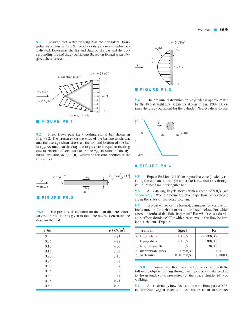
9.1 Assume that water flowing past the equilateral trian-gular bar shown in Fig. P9.1 produces the pressure distributionsindicated. Determine the lift and drag on the bar and the cor-responding lift and drag coefficients 1based on frontal area2. Ne-glect shear forces.
9.2 Fluid flows past the two-dimensional bar shown inFig. P9.2. The pressures on the ends of the bar are as shown,and the average shear stress on the top and bottom of the baris Assume that the drag due to pressure is equal to the dragdue to viscous effects. (a) Determine in terms of the dy-namic pressure, (b) Determine the drag coefficient forthis object.
*9.3 The pressure distribution on the 1-m-diameter circu-lar disk in Fig. P9.3 is given in the table below. Determine thedrag on the disk.
9.4 The pressure distribution on a cylinder is approximatedby the two straight line segments shown in Fig. P9.4. Deter-mine the drag coefficient for the cylinder. Neglect shear forces.
9.5 Repeat Problem 9.1 if the object is a cone 1made by ro-tating the equilateral triangle about the horizontal axis throughits tip2 rather than a triangular bar.
9.6 A 17-ft-long kayak moves with a speed of s (seeVideo V9.2). Would a boundary layer type flow be developedalong the sides of the boat? Explain.
9.7 Typical values of the Reynolds number for various an-imals moving through air or water are listed below. For whichcases is inertia of the fluid important? For which cases do vis-cous effects dominate? For which cases would the flow be lam-inar; turbulent? Explain.
† 9.8 Estimate the Reynolds numbers associated with thefollowing objects moving through air: (a) a snow flake settlingto the ground, (b) a mosquito, (c) the space shuttle, (d) youwalking.
9.9 Approximately how fast can the wind blow past a 0.25-in.-diameter twig if viscous effects are to be of importance
5 ft/
rU 2/2.
tavg
tavg.
Problems ■ 609
p = 0.5 U2
U = 5 ft /s
p = –0.25 U2
b = length = 4 ft
Linear distribution
0.1 ft
ρ
ρ
■ F I G U R E P 9 . 1
U
Width = b
p =
10h
h
avgU2ρ τ
avgτ
1__2
p = –0.2 U2ρ1__2( )
■ F I G U R E P 9 . 2
r
D = 1m
p = p(r)
p = –5 kN/m2
U
■ F I G U R E P 9 . 3
900
– U2ρ
U2ρ
180, deg
1__2
p
θ
θ
U
■ F I G U R E P 9 . 4
r (m) p (kN )
0 4.34
0.05 4.28
0.10 4.06
0.15 3.72
0.20 3.10
0.25 2.78
0.30 2.37
0.35 1.89
0.40 1.41
0.45 0.74
0.50 0.0
/m2 Animal Speed Re
1a2 large whale 300,000,000
1b2 flying duck 300,000
1c2 large dragonfly 30,000
1d2 invertebrate larva 0.31e2 bacterium 0.00003 0.01 mm/s 1 mm/s
7 m/s
20 m/s
10 m/s

throughout the entire flow field 1i.e., 2? Explain. Repeatfor a 0.004-in.-diameter hair and a 6-ft-diameter smokestack.
9.10 A viscous fluid flows past a flat plate such that theboundary layer thickness at a distance 1.3 m from the leadingedge is 12 mm. Determine the boundary layer thickness at dis-tances of 0.20, 2.0, and 20 m from the leading edge. Assumelaminar flow.
9.11 If the upstream velocity of the flow in Problem 9.10is determine the kinematic viscosity of the fluid.
9.12 Water flows past a flat plate with an upstream veloc-ity of Determine the water velocity a distanceof 10 mm from the plate at distances of and
from the leading edge.
*9.13 A Pitot tube connected to a water-filled U-tubemanometer is used to measure the total pressure within a bound-ary layer. Based on the data given in the table below, determinethe boundary layer thickness, the displacement thickness,and the momentum thickness,
9.14 Because of the velocity deficit, in the bound-ary layer, the streamlines for flow past a flat plate are not ex-actly parallel to the plate. This deviation can be determined byuse of the displacement thickness, For air blowing past theflat plate shown in Fig. P9.14, plot the streamline A–B thatpasses through the edge of the boundary layer at point B. That is, plot for streamline A–B. Assumelaminar boundary layer flow.
9.15 Air enters a square duct through a 1-ft opening as isshown in Fig. P9.15. Because the boundary layer displacementthickness increases in the direction of flow, it is necessary toincrease the cross-sectional size of the duct if a constant
velocity is to be maintained outside the boundary
layer. Plot a graph of the duct size, d, as a function of x forif U is to remain constant. Assume laminar flow.
9.16 A smooth, flat plate of length and widthis placed in water with an upstream velocity of
Determine the boundary layer thickness and thewall shear stress at the center and the trailing edge of the plate.Assume a laminar boundary layer.
9.17 An atmospheric boundary layer is formed when thewind blows over the earth’s surface. Typically, such velocityprofiles can be written as a power law: where the con-stants a and n depend on the roughness of the terrain. As is in-dicated in Fig. P9.17, typical values are for urban ar-eas, for woodland or suburban areas, and for flat open country 1Ref. 232. (a) If the velocity is 20 ftys atthe bottom of the sail on your boat what is the ve-locity at the top of the mast (b) If the average ve-locity is 10 mph on the tenth floor of an urban building, whatis the average velocity on the sixtieth floor?
9.18 A 30-story office building 1each story is 12 ft tall2 isbuilt in a suburban industrial park. Plot the dynamic pressure,
as a function of elevation if the wind blows at hurricanestrength 175 mph2 at the top of the building. Use the atmos-pheric boundary layer information of Problem 9.17.
9.19 The typical shape of small cumulus clouds is as indi-cated in Fig. P9.19. Based on boundary layer ideas, explain whyit is clear that the wind is blowing from right to left as indicated.
9.20 Show that by writing the velocity in terms of the simi-larity variable and the function the momentum equa-tion for boundary layer flow on a flat plate 1Eq. 9.92 can be writ-ten as the ordinary differential equation given by Eq. 9.14.
*9.21 Integrate the Blasius equation 1Eq. 9.142 numericallyto determine the boundary layer profile for laminar flow past aflat plate. Compare your results with those of Table 9.1.
f 1h2,h
ru2/2,
1y 5 30 ft2?1y 5 4 ft2,n 5 0.16n 5 0.28
n 5 0.40
u 5 ayn,
U 5 0.5 m/s.b 5 4 m
/ 5 6 m
0 # x # 10 ft
U 5 2 ft/s
y 5 y1x2 1y 5 dB at x 5 /2d*.
U 2 u,
™.d*,d,
x 5 15 mx 5 1.5 m
U 5 0.02 m/s.
U 5 1.5 m/s,
Re 6 1
610 ■ Chapter 9 / Flow Over Immersed Bodies
y (mm), h (mm),distance above plate manometer reading
0 0
2.1 10.6
4.3 21.1
6.4 25.6
10.7 32.5
15.0 36.9
19.3 39.4
23.6 40.5
26.8 41.0
29.3 41.0
32.7 41.0
yU =1 m/s
x
, = 4 m
Edge of boundary layer
Streamline A–B
δB
B
A
■ F I G U R E P 9 . 1 4
1 ft d(x) 2 ft/s
U =2 ft/s
x
■ F I G U R E P 9 . 1 5
u ~ y0.40
u ~ y0.28
u ~ y0.16
450
300
150
0
y, m
■ F I G U R E P 9 . 1 7

9.22 An airplane flies at a speed of 400 mph at an altitudeof 10,000 ft. If the boundary layers on the wing surfaces be-have as those on a flat plate, estimate the extent of laminarboundary layer flow along the wing. Assume a transitionalReynolds number of If the airplane maintainsits 400-mph speed but descends to sea level elevation, will theportion of the wing covered by a laminar boundary layerincrease or decrease compared with its value at 10,000 ft?Explain.
† 9.23 If the boundary layer on the hood of your car be-haves as one on a flat plate, estimate how far from the frontedge of the hood the boundary layer becomes turbulent. Howthick is the boundary layer at this location?
9.24 A laminar boundary layer velocity profile is approxi-mated by for and for
(a) Show that this profile satisfies the appropriate bound-ary conditions. (b) Use the momentum integral equation to de-termine the boundary layer thickness,
9.25 A laminar boundary layer velocity profile is approxi-mated by the two straight-line segments indicated in Fig. P9.25.Use the momentum integral equation to determine the bound-ary layer thickness, and wall shear stress,Compare these results with those in Table 9.2.
*9.26 An assumed, dimensionless laminar boundary layerprofile for flow past a flat plate is given in the table below. Usethe momentum integral equation to determine Compare your result with the exact Blasius solution result 1seeTable 9.22.
*9.27 For a fluid of specific gravity flowing pasta flat plate with an upstream velocity of the wallshear stress on a flat plate was determined to be as indicated inthe table below. Use the momentum integral equation to deter-mine the boundary layer momentum thickness, As-sume at the leading edge,
9.28 The square, flat plate shown in Fig. P9.28a is cutinto four equal-sized prices and arranged as shown in Fig.P9.28b. Determine the ratio of the drag on the original plate[case (a)] to the drag on the plates in the configuration shownin (b). Assume laminar boundary flow. Explain your answerphysically.
9.29 A plate is oriented parallel to the free stream as is in-dicated in Fig. 9.29. If the boundary layer flow is laminar, de-termine the ratio of the drag for case (a) to that for case (b).Explain your answer physically.
9.30 If the drag on one side of a flat plate parallel to theupstream flow is when the upstream velocity is U, what willthe drag be when the upstream velocity is 2U; or Assumelaminar flow.
U/2?d
x 5 0.™ 5 0™ 5 ™ 1x2.
U 5 5 m/s,SG 5 0.86
d 5 d1x2.
tw 5 tw1x2.d 5 d1x2,
d 5 d1x2.y 7 d.
u 5 Uy # d,u/U 5 32 2 1y/d2 4 1y/d2
Rexcr 5 5 3 105.
Problems ■ 611
y
δ
δ /2
u
U0 2U___3
■ F I G U R E P 9 . 2 5
U
■ F I G U R E P 9 . 1 9
0 0
0.080 0.133
0.16 0.265
0.24 0.394
0.32 0.517
0.40 0.630
0.48 0.729
0.56 0.811
0.64 0.876
0.72 0.923
0.80 0.956
0.88 0.976
0.96 0.988
1.00 1.000
u/Uy/D
x (m) (Ny )
0 —
0.2 13.4
0.4 9.25
0.6 7.68
0.8 6.51
1.0 5.89
1.2 6.57
1.4 6.75
1.6 6.23
1.8 5.92
2.0 5.26
m2Tw
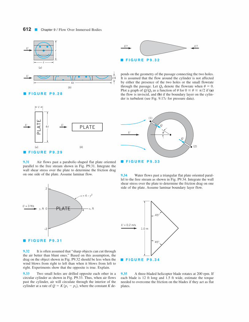
612 ■ Chapter 9 / Flow Over Immersed Bodies
9.31 Air flows past a parabolic-shaped flat plate orientedparallel to the free stream shown in Fig. P9.31. Integrate thewall shear stress over the plate to determine the friction dragon one side of the plate. Assume laminar flow.
9.32 It is often assumed that “sharp objects can cut throughthe air better than blunt ones.” Based on this assumption, thedrag on the object shown in Fig. P9.32 should be less when thewind blows from right to left than when it blows from left toright. Experiments show that the opposite is true. Explain.
9.33 Two small holes are drilled opposite each other in acircular cylinder as shown in Fig. P9.33. Thus, when air flowspast the cylinder, air will circulate through the interior of thecylinder at a rate of where the constant K de-
pends on the geometry of the passage connecting the two holes.It is assumed that the flow around the cylinder is not affectedby either the presence of the two holes or the small flowratethrough the passage. Let denote the flowrate when Plot a graph of as a function of for if (a)
the flow is inviscid, and (b) if the boundary layer on the cylin-der is turbulent (see Fig. 9.17c for pressure data).
9.34 Water flows past a triangular flat plate oriented paral-lel to the free stream as shown in Fig. P9.34. Integrate the wallshear stress over the plate to determine the friction drag on oneside of the plate. Assume laminar boundary layer flow.
9.35 A three-bladed helicopter blade rotates at 200 rpm. Ifeach blade is 12 ft long and 1.5 ft wide, estimate the torqueneeded to overcome the friction on the blades if they act as flatplates.
0 # u # p/2uQ/Q0
u 5 0.Q0
Q 5 K 1p1 2 p22,
U
U
,
4,
,
,/4
(b)
(a)
■ F I G U R E P 9 . 2 8
PL
AT
E
,
4,U U
PLATE
(a) (b)
■ F I G U R E P 9 . 2 9
2
0y, ft
–2
4
U = 3 ft/sx, ft
x = 4 – y2
PLATE
■ F I G U R E P 9 . 3 1
U? U?
■ F I G U R E P 9 . 3 2
U
(1)
Q
Q
θ
(2)
■ F I G U R E P 9 . 3 3
U = 0.2 m/s
1.0 m
45°
45°
■ F I G U R E P 9 . 3 4
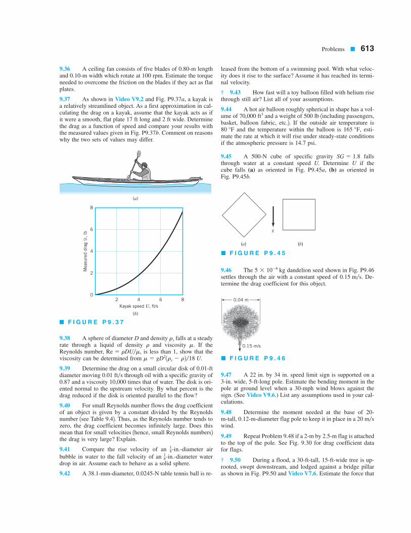
Problems ■ 613
9.36 A ceiling fan consists of five blades of 0.80-m lengthand 0.10-m width which rotate at 100 rpm. Estimate the torqueneeded to overcome the friction on the blades if they act as flatplates.
9.37 As shown in Video V9.2 and Fig. P9.37a, a kayak isa relatively streamlined object. As a first approximation in cal-culating the drag on a kayak, assume that the kayak acts as ifit were a smooth, flat plate 17 ft long and 2 ft wide. Determinethe drag as a function of speed and compare your results withthe measured values given in Fig. P9.37b. Comment on reasonswhy the two sets of values may differ.
9.38 A sphere of diameter D and density falls at a steadyrate through a liquid of density and viscosity If theReynolds number, is less than 1, show that theviscosity can be determined from
9.39 Determine the drag on a small circular disk of 0.01-ftdiameter moving through oil with a specific gravity of0.87 and a viscosity 10,000 times that of water. The disk is ori-ented normal to the upstream velocity. By what percent is thedrag reduced if the disk is oriented parallel to the flow?
9.40 For small Reynolds number flows the drag coefficientof an object is given by a constant divided by the Reynoldsnumber 1see Table 9.42. Thus, as the Reynolds number tends tozero, the drag coefficient becomes infinitely large. Does thismean that for small velocities 1hence, small Reynolds numbers2the drag is very large? Explain.
9.41 Compare the rise velocity of an -diameter air
bubble in water to the fall velocity of an -diameter waterdrop in air. Assume each to behave as a solid sphere.
9.42 A 38.1-mm-diameter, 0.0245-N table tennis ball is re-
leased from the bottom of a swimming pool. With what veloc-ity does it rise to the surface? Assume it has reached its termi-nal velocity.
† 9.43 How fast will a toy balloon filled with helium risethrough still air? List all of your assumptions.
9.44 A hot air balloon roughly spherical in shape has a vol-ume of and a weight of 500 lb 1including passengers,basket, balloon fabric, etc.2. If the outside air temperature is
and the temperature within the balloon is esti-mate the rate at which it will rise under steady-state conditionsif the atmospheric pressure is 14.7 psi.
9.45 A 500-N cube of specific gravity fallsthrough water at a constant speed U. Determine U if thecube falls (a) as oriented in Fig. P9.45a, (b) as oriented inFig. P9.45b.
9.46 The dandelion seed shown in Fig. P9.46settles through the air with a constant speed of De-termine the drag coefficient for this object.
9.47 A 22 in. by 34 in. speed limit sign is supported on a3-in. wide, 5-ft-long pole. Estimate the bending moment in thepole at ground level when a 30-mph wind blows against thesign. (See Video V9.6.) List any assumptions used in your cal-culations.
9.48 Determine the moment needed at the base of 20-m-tall, 0.12-m-diameter flag pole to keep it in place in a wind.
9.49 Repeat Problem 9.48 if a 2-m by 2.5-m flag is attachedto the top of the pole. See Fig. 9.30 for drag coefficient datafor flags.
† 9.50 During a flood, a 30-ft-tall, 15-ft-wide tree is up-rooted, swept downstream, and lodged against a bridge pillaras shown in Fig. P9.50 and Video V7.6. Estimate the force that
20 m/s
0.15 m/s.5 3 1026 kg
SG 5 1.8
165 °F,80 °F
70,000 ft3
18-in.
18-in.
0.01 ft/s
m 5 gD21rs 2 r2/18 U.Re 5 rDU/m,
m.rrs
(a)
g
(b)
■ F I G U R E P 9 . 4 5
0.04 m
0.15 m/s
■ F I G U R E P 9 . 4 6
8
6
4
2
02 4
Kayak speed U, ft/s
6 8
Measu
red d
rag $
, lb
(b)
(a)
■ F I G U R E P 9 . 3 7
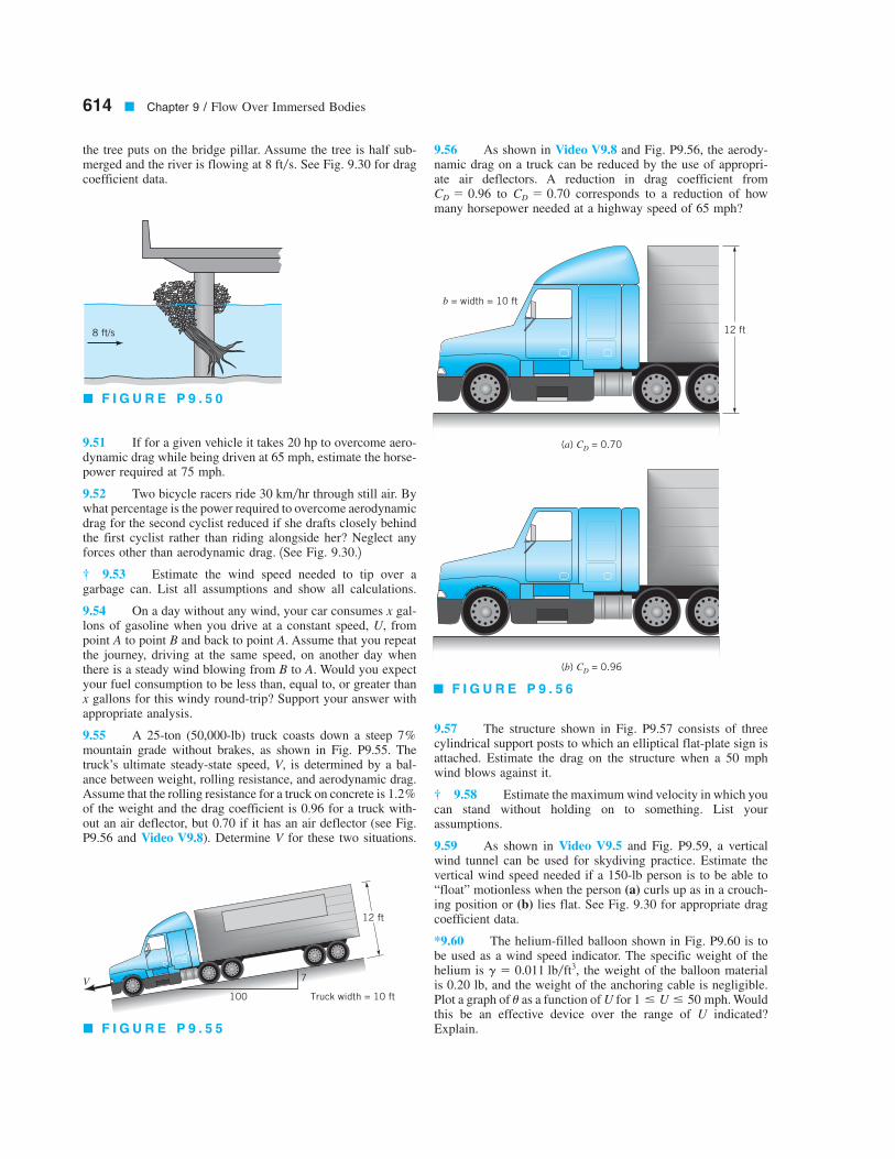
614 ■ Chapter 9 / Flow Over Immersed Bodies
the tree puts on the bridge pillar. Assume the tree is half sub-merged and the river is flowing at See Fig. 9.30 for dragcoefficient data.
9.51 If for a given vehicle it takes 20 hp to overcome aero-dynamic drag while being driven at 65 mph, estimate the horse-power required at 75 mph.
9.52 Two bicycle racers ride through still air. Bywhat percentage is the power required to overcome aerodynamicdrag for the second cyclist reduced if she drafts closely behindthe first cyclist rather than riding alongside her? Neglect anyforces other than aerodynamic drag. 1See Fig. 9.30.2† 9.53 Estimate the wind speed needed to tip over agarbage can. List all assumptions and show all calculations.
9.54 On a day without any wind, your car consumes x gal-lons of gasoline when you drive at a constant speed, U, frompoint A to point B and back to point A. Assume that you repeatthe journey, driving at the same speed, on another day whenthere is a steady wind blowing from B to A. Would you expectyour fuel consumption to be less than, equal to, or greater thanx gallons for this windy round-trip? Support your answer withappropriate analysis.
9.55 A 25-ton (50,000-lb) truck coasts down a steep mountain grade without brakes, as shown in Fig. P9.55. Thetruck’s ultimate steady-state speed, V, is determined by a bal-ance between weight, rolling resistance, and aerodynamic drag.Assume that the rolling resistance for a truck on concrete is of the weight and the drag coefficient is 0.96 for a truck with-out an air deflector, but 0.70 if it has an air deflector (see Fig.P9.56 and Video V9.8). Determine V for these two situations.
9.56 As shown in Video V9.8 and Fig. P9.56, the aerody-namic drag on a truck can be reduced by the use of appropri-ate air deflectors. A reduction in drag coefficient from
to corresponds to a reduction of howmany horsepower needed at a highway speed of 65 mph?
9.57 The structure shown in Fig. P9.57 consists of threecylindrical support posts to which an elliptical flat-plate sign isattached. Estimate the drag on the structure when a 50 mphwind blows against it.
† 9.58 Estimate the maximum wind velocity in which youcan stand without holding on to something. List yourassumptions.
9.59 As shown in Video V9.5 and Fig. P9.59, a verticalwind tunnel can be used for skydiving practice. Estimate thevertical wind speed needed if a 150-lb person is to be able to“float” motionless when the person (a) curls up as in a crouch-ing position or (b) lies flat. See Fig. 9.30 for appropriate dragcoefficient data.
*9.60 The helium-filled balloon shown in Fig. P9.60 is tobe used as a wind speed indicator. The specific weight of thehelium is the weight of the balloon materialis 0.20 lb, and the weight of the anchoring cable is negligible.Plot a graph of as a function of U for Wouldthis be an effective device over the range of U indicated?Explain.
1 # U # 50 mph.u
g 5 0.011 lb/ft3,
CD 5 0.70CD 5 0.96
1.2%
7%
30 km/hr
8 ft/s.
8 ft/s
■ F I G U R E P 9 . 5 0
100
7
Truck width = 10 ft
12 ft
V
■ F I G U R E P 9 . 5 5
(a) CD = 0.70
b = width = 10 ft
(b) CD = 0.96
12 ft
■ F I G U R E P 9 . 5 6
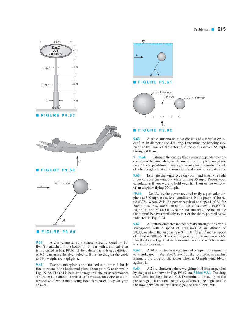
Problems ■ 615
9.61 A 2-in.-diameter cork sphere 1specific weight2 is attached to the bottom of a river with a thin cable, as
is illustrated in Fig. P9.61. If the sphere has a drag coefficientof 0.5, determine the river velocity. Both the drag on the cableand its weight are negligible.
9.62 Two smooth spheres are attached to a thin rod that isfree to rotate in the horizontal plane about point O as shown inFig. P9.62. The rod is held stationary until the air speed reaches
Which direction will the rod rotate 1clockwise or coun-terclockwise2 when the holding force is released? Explain youranswer.
9.63 A radio antenna on a car consists of a circular cylin-der in. in diameter and 4 ft long. Determine the bending mo-ment at the base of the antenna if the car is driven 55 mphthrough still air.
† 9.64 Estimate the energy that a runner expends to over-come aerodynamic drag while running a complete marathonrace. This expenditure of energy is equivalent to climbing a hillof what height? List all assumptions and show all calculations.
9.65 Estimate the wind force on your hand when you holdit out of your car window while driving 55 mph. Repeat yourcalculations if you were to hold your hand out of the windowof an airplane flying 550 mph.
*9.66 Let be the power required to fly a particular air-plane at 500 mph at sea level conditions. Plot a graph of the ra-tio where is the power required at a speed of U, for
at altitudes of sea level, 10,000 ft,20,000 ft, and 30,000 ft. Assume that the drag coefficient forthe aircraft behaves similarly to that of the sharp-pointed ogiveindicated in Fig. 9.24.
9.67 A 0.50-m-diameter meteor streaks through the earth’satmosphere with a speed of at an altitude of 20,000 m where the air density is and the speedof sound is The specific gravity of the meteor is 7.65.Use the data in Fig. 9.24 to determine the rate at which the me-teor is decelerating.
9.68 A 30-ft-tall tower is constructed of equal 1-ft segmentsas is indicated in Fig. P9.68. Each of the four sides is similar.Estimate the drag on the tower when a 75-mph wind blowsagainst it.
9.69 A 2-in.-diameter sphere weighing 0.14 lb is suspendedby the jet of air shown in Fig. P9.69 and Video V3.1. The dragcoefficient for the sphere is 0.5. Determine the reading on thepressure gage if friction and gravity effects can be neglected forthe flow between the pressure gage and the nozzle exit.
300 m/s.9 3 1022 kg/m
31800 m/s
500 mph # U # 3000 mphpp/p0,
p0
14
50 ft/s.
lb/ft3
5 13
10 ft
0.6 ft
0.8 ft
1 ft 15 ft
15 ft
15 ft
5 ft
■ F I G U R E P 9 . 5 7
U
■ F I G U R E P 9 . 5 9
60°
U
■ F I G U R E P 9 . 6 1
U
1.5-ft diameter
0.7-ft diameterO (pivot)
, ,
■ F I G U R E P 9 . 6 2
U2-ft diameter
θ
■ F I G U R E P 9 . 6 0

616 ■ Chapter 9 / Flow Over Immersed Bodies
9.70 The United Nations Building in New York is approx-imately 87.5-m wide and 154-m tall. (a) Determine the drag onthis building if the drag coefficient is 1.3 and the wind speedis a uniform (b) Repeat your calculations if the veloc-ity profile against the building is a typical profile for an urbanarea 1see Problem 9.172 and the wind speed halfway up thebuilding is
† 9.71 An “air-popper” popcorn machine blows hot airpast the kernels with speed U so that the unpopped ones remainin the holder but the popped kernels are blown outof the holder Estimate the range of air velocity al-lowed for proper operation of the machine List all assumptions and show all calculations.
9.72 When the 0.9-lb box kite shown in Fig. P9.72 is flownin a wind, the tension in the string, which is at a an-gle relative to the ground, is 3.0 lb. (a) Determine the lift anddrag coefficients for the kite based on the frontal area of (b) If the wind speed increased to would the kite riseor fall? That is, would the angle shown in the figure in-crease or decrease? Assume the lift and drag coefficients re-main the same. Support your answer with appropriate calcula-tions.
9.73 A regulation football is 6.78 in. in diameter and weighs0.91 lb. If its drag coefficient is determine its decel-eration if it has a speed of at the top of its trajectory.
9.74 Explain how the drag on a given smokestack could bethe same in a 2 mph wind as in a 4 mph wind. Assume the val-ues of and are the same for each case.
9.75 The faster a baseball bat is swung, the farther the ballwill travel when hit by the bat. If the aerodynamic drag on thebat can be reduced, the bat can be swung faster. As discussedin Section 9.3, the drag on dimpled golf balls is less than thaton equal-sized smooth balls. Thus, does it follow that dimpleson baseball bats can increase the distance that balls are hit? Ex-plain your answer.
† 9.76 If the wind becomes strong enough, it is “impos-sible” to paddle a canoe into the wind. Estimate the wind speedat which this will happen. List all assumptions and show all cal-culations.
9.77 A strong wind can blow a golf ball off the tee by piv-oting it about point 1 as shown in Fig. P9.77. Determine thewind speed necessary to do this.
9.78 An airplane tows a banner that is tall andlong at a speed of If the drag coefficient
based on the area is estimate the power requiredto tow the banner. Compare the drag force on the banner withthat on a rigid flat plate of the same size. Which has the largerdrag force and why?
9.79 By appropriate streamlining, the drag coefficient foran airplane is reduced by 12% while the frontal area remainsthe same. For the same power output, by what percentage is theflight speed increased?
CD 5 0.06,b/150 km/hr./ 5 25 m
b 5 0.8 m
mr
20 ft/sCD 5 0.2,
30°30 ft/s,
6.0 ft2.
30°20 ft/s
1Umin 6 U 6 Umax2.1U 7 Umin2.1U 6 Umax2,
20 m/s.
20 m/s.
2 in.
1 in.
1 in.
1 ft
1 ft
■ F I G U R E P 9 . 6 8
Air
Area = 0.6 ft2
Area = 0.3 ft2
Pressure
gage
■ F I G U R E P 9 . 6 9
U = 20 ft/s
30°
T = 3 lb
■ F I G U R E P 9 . 7 2
0.20 in.
Weight = 0.0992 lb
Radius = 0.845 in.
(1)
U
■ F I G U R E P 9 . 7 7

Problems ■ 617
9.80 The dirigible Akron had a length of 239 m and a max-imum diameter of 40.2 m. Estimate the power required at itsmaximum speed of if the drag coefficient based onfrontal area is 0.060.
9.81 Estimate the power needed to overcome the aerody-namic drag of a person who runs at a rate of 100 yds in 10 sin still air. Repeat the calculations if the race is run into a 20-mph headwind; a 20-mph tailwind. Explain.
† 9.82 Skydivers often join together to form patterns dur-ing the free-fall portion of their jump. The current Guiness Bookof World Records record is 297 skydivers joined hand-to-hand.Given that they can’t all jump from the same airplane at thesame time, describe how they manage to get together (see VideoV9.5). Use appropriate fluid mechanics equations and princi-ples in your answer.
9.83 A fishnet consists of 0.10-in.-diameter strings tiedinto squares 4 in. per side. Estimate the force needed to tow a15-ft by 30-ft section of this net through seawater at
9.84 An iceberg floats with approximately of its volumein the air as is shown in Fig. P9.84. If the wind velocity is Uand the water is stationary, estimate the speed at which the windforces the iceberg through the water.
9.85 A Piper Cub airplane has a gross weight of 1750 lb,a cruising speed of 115 mph, and a wing area of . De-termine the lift coefficient of this airplane for these conditions.
9.86 A light aircraft with a wing area of and a weightof 2000 lb has a lift coefficient of 0.40 and a drag coefficientof 0.05. Determine the power required to maintain level flight.
9.87 As shown in Video V9.9 and Fig. P9.87, a spoiler isused on race cars to produce a negative lift, thereby giving abetter tractive force. The lift coefficient for the airfoil shown is
, and the coefficient of friction between the wheels andthe pavement is 0.6. At a speed of 200 mph, by how much woulduse of the spoiler increase the maximum tractive force that couldbe generated between the wheels and ground? Assume the airspeed past the spoiler equals the car speed and that the airfoilacts directly over the drive wheels.
9.88 The wings of old airplanes are often strengthened bythe use of wires that provided cross-bracing as shown inFig. P9.88. If the drag coefficient for the wings was 0.020 1basedon the planform area2, determine the ratio of the drag from thewire bracing to that from the wings.
9.89 The jet engines on a Boeing 757 must develop a cer-tain amount of power to propel the airplane through the air witha speed of 570 mph at a cruising altitude of 35,000 ft. By whatpercent must the power be increased if the same airplane wereto maintain its 570 mph flight speed at sea level?
9.90 A wing generates a lift when moving through sealevel air with a velocity U. How fast must the wing movethrough the air at an altitude of 35,000 ft with the same lift co-efficient if it is to generate the same lift?
*9.91 When air flows past the airfoil shown in Fig. P9.91,the velocity just outside the boundary layer, u, is as indicated.Estimate the lift coefficient for these conditions.
l
CL 5 1.1
200 ft2
179 ft2
17
5 ft/s.
135 km/hrakkjbgfkgbsgboiabkv
GOOD YEAR
A manufacturer of fine clothing and accessories
33sfglfbkjxfdbaerg
200 mph
Spoiler 1.5 ft
b = spoiler length = 4 ft
■ F I G U R E P 9 . 8 7
Speed: 70 mph
Wing area: 148 ft2
Wire: length = 160 ft
diameter = 0.05 in.
■ F I G U R E P 9 . 8 8
1.6
1.2
0.8
0.4
00 0.2 0.4 0.6 0.8 1.0
x__c
u__U
U
uNACA 632–015
Lower surface
Upper surface
( )2
■ F I G U R E P 9 . 9 1
U
volume in water6__7
volume in air1__7
■ F I G U R E P 9 . 8 4

618 ■ Chapter 9 / Flow Over Immersed Bodies
9.92 To help ensure safe flights, air-traffic controllers en-force a minimum time interval between takeoffs. During busytimes this can result in a long queue of aircraft waiting for take-off clearance. Based on the flow shown in Fig. 9.37 and Videos4.2, 9.1, and 9.9, explain why the interval between takeoffs canbe shortened if the wind has a cross-runway component (as op-posed to blowing directly down the runway).
9.93 A Boeing 747 aircraft weighing 580,000 lb whenloaded with fuel and 100 passengers takes off with an airspeedof 140 mph. With the same configuration 1i.e., angle of attack,flap settings, etc.2, what is its takeoff speed if it is loaded with372 passengers? Assume each passenger with luggage weighs200 lb.
9.94 Show that for unpowered flight 1for which the lift,drag, and weight forces are in equilibrium2 the glide slope an-gle, is given by
9.95 If the lift coefficient for a Boeing 777 aircraft is 15times greater than its drag coefficient, can it glide from an al-titude of 30,000 ft to an airport 80 mi away if it loses powerfrom its engines? Explain. 1See Problem 9.94.29.96 On its final approach to the airport, an airplane flieson a flight path that is relative to the horizontal. What lift-to-drag ratio is needed if the airplane is to land with its enginesidled back to zero power? 1See Problem 9.94.29.97 A sail plane with a lift-to-drag ratio of 25 flies with aspeed of 50 mph. It maintains or increases its altitude by fly-ing in thermals, columns of vertically rising air produced bybuoyancy effects of nonuniformly heated air. What vertical air-speed is needed if the sail plane is to maintain a constant alti-tude?
9.98 Over the years there has been a dramatic increase inthe flight speed (U ) and altitude (h), weight and wingloading ( divided by wing area) of aircraft. Usethe data given in the table below to determine the lift coeffi-cient for each of the aircraft listed.
9.99 The landing speed of an airplane such as the SpaceShuttle is dependent on the air density. (See Video V9.1.) Bywhat percent must the landing speed be increased on a day whenthe temperature is compared to a day when it is Assume that the atmospheric pressure remains constant.
9.100 Commercial airliners normally cruise at relativelyhigh altitudes 130,000 to 35,000 ft2. Discuss how flying at thishigh altitude 1rather than 10,000 ft, for example2 can save fuelcosts.
9.101 A pitcher can pitch a “curve ball” by puttingsufficient spin on the ball when it is thrown. A ball that hasabsolutely no spin will follow a “straight” path. A ball that ispitched with a very small amount of spin 1on the order of onerevolution during its flight between the pitcher’s mound andhome plate2 is termed a knuckle ball. A ball pitched this waytends to “jump around” and “zig-zag” back and forth. Explainthis phenomenon. Note: A baseball has seams.
9.102 Repeated controversy regarding the ability of a base-ball to curve appeared in the literature for years. According toa test 1Life, July 27, 19532, a baseball 1assume the diameter is2.9 in. and weight is 5.25 oz2 spinning 1400 rpm while travel-ing 43 mph was observed to follow a path with an 800-ft hor-izontal radius of curvature. Based on the data of Fig. 9.39, doyou agree with this test result? Explain.
9.103 This problem involves measuring the boundary layerprofile on a flat plate. To proceed with this problem, click herein the E-book.
9.104 This problem involves measuring the pressure distri-bution on a circular cylinder. To proceed with this problem,click here in the E-book.
50 °F?110 °F
w/A 5 weight1w2,
3.0°
tan u 5 CD/CL.u,
Aircraft Year , lb U, mph h, ft
Wright Flyer 1903 750 35 1.5 0Douglas DC-3 1935 25,000 180 25.0 10,000Douglas DC-6 1947 105,000 315 72.0 15,000Boeing 747 1970 800,000 570 150.0 30,000
w/A, lb/ft2
w
Copyright © 2022 FDOKUMEN