Modelling and simulation

of porous immersed boundaries

John M. Stockie ∗

Department of Mathematics, Simon Fraser University, 8888 University Drive,

Burnaby, BC, V5A 1S6, Canada

Abstract

The immersed boundary method has been used to simulate a wide range of fluid-structure interaction problems from biology and engineering, wherein flexible solidstructures deform in response to a surrounding incompressible fluid flow. We gen-eralize the IB method to handle porous membranes by incorporating an additionaltransmembrane flux that obeys Darcy’s law. An approximate analytical solutionis derived that clearly illustrates the effect of porosity on the immersed boundarymotion. Numerical simulations in two dimensions are used to validate the analyticalresults and to illustrate the motion of more general porous membrane dynamics.

Key words: Immersed boundary method, Porous membrane, Fluid-structureinteraction, Volume conservation

1 Introduction

The immersed boundary (IB) method has proven to be a versatile and robustapproach for simulating the interaction of complex, deformable, solid struc-tures with an underlying incompressible fluid flow [23]. The method has beenapplied extensively to problems arising in bio-fluid dynamics, including bloodflow in the heart [24] and arteries [1], biofilms [11], and swimming dynamicsof flagellated cells, worms, and other organisms [7]. The IB method has alsobeen utilized for non-biological fluid-structure interaction problems such assuspension flows [27] and parachute dynamics [16].

∗ Tel: +1 778 782 3553. Fax: +1 778 782 4947.Email address: stockie@math.sfu.ca (John M. Stockie).

Preprint submitted to Elsevier 1 February 2009

The subject of this paper is a class of fluid-structure interaction problemswherein the deformable boundary is also porous, permitting the fluid to flowthrough it in response to transmural pressure gradients. Such porous immersedboundaries abound in biological systems, including such examples as arterywalls [13], brain tissue [26], lipid vesicles and cell membranes [14], and also ap-pear in engineering applications such as ocean wave barriers [5,15] or filtrationand separation processes. Most existing numerical methods for simulating flowthrough porous boundaries assume that the boundary is stationary and doesnot deform in response to the flow, even though the deformations encounteredin actual applications can be substantial; therefore, there is much to be gainedby generalizing the IB method to include the effects of porosity.

The only previous attempt to incorporate porosity within the IB frameworkis a study of parachute dynamics by Kim and Peskin [16] wherein the airvents at the apex of the chute were dealt with by allowing the normal velocityof the canopy to differ from that of the fluid by an amount proportionalto the normal component of the boundary force. The IB method has alsobeen used to study flow through granular media at the pore scale by treatingthe grains making up the medium as immersed boundaries [10], although thegrains themselves are rigid and impermeable in these studies. In a study ofporous cell membrane transport, Layton [18] generalized the closely-relatedimmersed interface method by introducing a porous slip velocity in the normaldirection that is driven by differences in both transmural water pressure andsolute concentration. However, to date there has been no systematic study ofporosity in the context of the IB method.

Our aim in this paper is to extend the IB method to handle porous immersedboundaries in a way that is easily implemented for use in applications. Ourtreatment is restricted to two dimensions although the extension to 3D isstraightforward. We follow Kim and Peskin’s approach [16] by incorporating anormal porous slip velocity into the boundary evolution equation. The modelequations are presented in Section 2 after which we derive an explicit analyti-cal solution for the special case of a circular membrane subject only to porousleakage. The numerical algorithm is outlined in Section 3, which demonstratesthat extending existing IB codes using our approach is straightforward. InSection 4, we draw a connection between errors in volume conservation thatare inherent in non-porous IB computations, and the leakage through porousmembranes. In particular, these volume errors may be viewed as deriving froman intrinsic permeability in the discretized immersed boundary. We investigatethe implications of this hypothesis in some detail and are led naturally to amodification of the IB method that corrects for volume errors by introducingan additional porous correction term. Numerical simulations are presented inSection 5 that validate our analytical solution, illustrate more complex porousmembrane dynamics, and evaluate our proposed technique for improving vol-ume conservation.

2

2 Mathematical Formulation

We begin by presenting the equations governing the motion of a non-porousboundary immersed in a fluid, following the notation introduced by Peskin [23].We consider a two-dimensional fluid domain Ω within which is suspended asingle immersed boundary or membrane that can be described by a continuous,non-intersecting curve Γ. The state of the fluid at any position ~x = (x, y) (ins) and time t (s) is described by the velocity ~u(~x, t) (cm/s) and pressurep(~x, t) (g/cm s2), which are assumed to obey the incompressible Navier-Stokesequations

ρ (~ut + ~u · ∇~u) = µ∆~u −∇p + ~f, (1)

∇ · ~u = 0. (2)

The parameters appearing in the above are the density ρ (g/cm3) and dynamicviscosity µ (g/cm s), both of which are taken to be constant.

The function ~f(~x, t) represents the force exerted by the membrane per unitvolume of fluid (g/cm2 s2), and is dependent on the current configuration of

the membrane. The membrane position is denoted ~X(s, t) = (X(s, t), Y (s, t))where s is a parameterization of the curve in some reference configuration,and so the fluid force may be written as

~f(~x, t) =∫

Γ

~F (s, t) δ(~x − ~X(s, t)) ds, (3)

where δ(~x) is the two-dimensional delta function. The function ~F (g/s2),representing the immersed boundary force per unit length, may be writ-ten as ~F = (T ~τ)s where T (s, t) is the tension within the membrane and

~τ (s, t) = ~Xs/| ~Xs| is the unit tangent vector. For the simple case of a linearelastic material that resists both stretching and compression, the membranetension takes the form T = σ(| ~Xs| − R) where the equilibrium state of the

membrane is given by ~Xs = R for R some constant, and σ (g/cm s2) repre-sents the spring constant of the material. With the above definitions, the forcedensity becomes

~F = σ[~Xs

(1 − R/| ~Xs|

)]

s, (4)

which is a nonlinear function of the IB position ~X except in the special caseof a membrane with zero resting where Eq. (4) reduces to ~F = σ ~Xss.

In order to close the system, an equation governing the membrane motion isrequired. According to the no-slip condition the membrane must move at the

3

same velocity as neighbouring fluid particles, which requires that

~Xt = ~u( ~X(s, t), t),

which is conveniently written in terms of a delta-function convolution as

~Xt =∫

Ω~u(~x, t) δ(~x − ~X(s, t)) d~x. (5)

It is important to note the presence of the delta functions in both Eqs. (3)and (5), which leads us naturally to a simple and efficient numerical schemethat will be described in detail in Section 3.

2.1 Immersed Boundaries with Porosity

The system of equations (1)–(5) is now generalized to include the effect ofporosity in Γ. We follow the approach used by Kim and Peskin [16], whoincorporated the effect of air vents in a parachute canopy by introducing aporous slip velocity that accounts for air leakage through the vents. The porousflux is directed normal to the chute and is driven by a difference in air pressurefrom one side to the other – this is a reasonable assumption if the “pores” aredirected normally to the chute and have diameter that is small relative totheir length. The porous slip velocity can then be expressed as Up ~n where

~n = ~τ × ~e3 = (Xs,−Ys)/| ~Xs| is the unit normal vector to Γ, Up is given byDarcy’s law [4] as

Up(s, t) = −K [[p]]

µa, (6)

and [[p]] = p|Γ+ − p|Γ− denotes the jump in pressure. Among the parametersappearing in the above expression, K represents the membrane permeability(cm2) and a is the membrane thickness (cm).

The introduction of a pressure jump in (6) may seem at first to be a significantcomplication since it introduces a coupling to the momentum equations (1)through the unknown pressure. However, as is demonstrated in [25], Eq. (1)may be integrated to eliminate the delta-function forcing term and obtaininstead the following expressions for the jumps in normal and tangential fluidstress across the membrane:

− [[p]] + µ~n ·[[

∂~u

∂n

]]= −

~F · ~n| ~Xs|

and µ~τ ·[[

∂~u

∂n

]]= −

~F · ~τ| ~Xs|

. (7)

The first jump condition may be simplified using the incompressibility condi-

4

tion (2) to obtain

[[p]] =~F · ~n| ~Xs|

, (8)

which may be used to rewrite the porous slip velocity in Eq. (6) in terms ofthe IB force density

Up(s, t) = −α~F · ~n| ~Xs|

, (9)

where the constant α = Kµa

has units of cm2 s/g. The porous membrane obeys

the same governing equations (1)–(4) as in the non-porous case, except thatthe boundary evolution equation is replaced with

~Xt = −Up ~n +∫

Ω~u(~x, t) δ(~x − ~X(s, t)) d~x, (10)

We note that Kim and Peskin’s formulation [16] is equivalent to our own if

we replace our porous slip parameter α with βγ/| ~Xs|, where β is the numberdensity of pores and γ is the aerodynamic conductance of the membrane. Themain difference between their approach and our own is that we have madeexplicit use of Darcy’s law which permits us to express α in terms of thepermeability K, a parameter that is easily obtained from experiments. Theparameters β and γ, on the other hand, are not commonly available in theporous media literature.

Finally, we close by mentioning the work of Layton [18] who used a similarapproach to incorporate porosity into the related immersed interface method,the primary difference being that her method makes explicit use of the stressjump conditions instead of delta function convolutions.

2.2 A Simple Analytical Solution

We next derive an explicit analytical solution to the porous IB problem in thecase of a circular (radially-symmetric) membrane, centered at the origin in afluid of infinite extent. To this end, we assume that the unstressed equilibriumstate of the membrane is a circle with radius Req ≥ 0. Then the membraneconfiguration at any time t can be written as

~X(s, t) = r(t) [cos s, sin s], (11)

where the parameter s ∈ [0, 2π] corresponds to the polar angle and is measuredcounter-clockwise around the membrane. The other membrane quantities ap-

5

pearing in the IB equations may then be expressed as

~Xs = r(t)[− sin s, cos s], ~τ = [− sin s, cos s],∣∣∣ ~Xs

∣∣∣ = r(t), ~n = [cos s, sin s].

The membrane resting length in Eq. (4) must be R = Req in order that theforce density at the equilibrium state vanishes; consequently,

~F = σ(Req − r)~n, (12)

and the Darcy velocity from Eq. (9) becomes

Up(s, t) = ασ

(1 − Req

r(t)

). (13)

A simple thought experiment can be used to verify that this velocity behaves asexpecte: when r(t) > Req the membrane is stretched which causes the pressureto be higher inside the membrane and consequently results in the interior fluidleaking outwards (i.e., Up > 0). The opposite is true when r(t) < Req, andwhen r(t) = Req the Darcy velocity is identically zero, which implies thatthere is no porous leakage at the equilibrium state.

If we assume that the fluid velocity is small enough that contributions to thedynamics from the underlying fluid flow are negligible, then the membranemotion is driven primarily by porous effects and Eq. (10) can be approximatedby dr/dt ≈ −Up. Then, according to Eq. (13), r(t) satisfies the followingordinary differential equation

dr

dt= −ασ

(1 − Req

r

). (14)

When this equation is supplemented by the initial condition r(0) = Ro an ex-plicit analytical solution may be obtained, which we separate into the followingtwo cases.

Case 1, Req = 0: For a membrane with a zero resting length, Eq. (14) re-duces to dr/dt = −ασ which has exact solution

r(t) =

Ro − ασt, if t < Ro/ασ,

0, otherwise.(15)

The solution is truncated at time t = Ro/ασ, beyond which the radius isidentically zero. This zero-volume steady state is only an idealization sincea physical membrane can never actually shrink to a point; nevertheless, itprovides an extremely useful test case for computations since it is easy tocompute the linear rate of decrease of the membrane radius. The solutionprofiles corresponding to ασ = 0.016 cm/s are displayed in Fig. 1 for several

6

choices of initial radius. If either σ or α were increased – corresponding toa stiffer or more porous membrane respectively – then the linear solutionprofiles would steepen, meaning that the membrane relaxes more rapidly tothe equilibrium state.

Case 2, Req > 0: In the more general case of a non-zero resting length, thesolution to Eq. (14) is

r(t) = Req

[1 + W (c exp[−ασt/Req])

], (16)

where c is a constant of integration, and W (x) is the Lambert W-functionwhich satisfies W (x) eW (x) = x (see [6] for an extensive of review of theproperties of W ). By applying the initial condition, we obtain the constant

c =

(Ro

Req

− 1

)exp

(Ro

Req

− 1

). (17)

We note that the rate of decay depends on the quantity ασ, just as in thecase Req = 0. The time evolution of an initially circular porous membranehaving equilibrium radius Req = 0.2 is displayed in Fig. 1 alongside theanalytical solution for Req = 0, keeping all other parameter values the same.The primary differences between this and the Req = 0 solution is that therate of decay to equilibrium is significantly slower, and the radius no longerbehaves linearly but rather more in an exponential fashion.

[Fig. 1 about here.]

3 Solution Algorithm

The algorithm we describe next is the original IB method proposed by Pe-skin [22] which is still commonly used especially in bio-fluid applications. Themethod can be viewed as a mixed Eulerian-Lagrangian approach, wherein thefluid unknowns are approximated on a fixed Cartesian grid and the membranequantities on a moving set of Lagrangian points. The fluid domain is assumedto be a square Ω = [0, L] × [0, L] and is discretized using a uniform N × Ngrid with spacing h = L/N in each direction. The time interval [0, T ] is di-vided into M equal sub-intervals of length k = T/M . The discrete velocityunknowns may then be written as ~un

i,j ≈ ~u(xi, yj, tn) where xi = ih, yj = jhfor i, j = 1, 2, . . . , N , and tn = nk for n = 1, 2, . . . , M (with similar approxi-

mations for the pressure pni,j and fluid force ~fn

i,j). The membrane variables, onthe other hand, are discretized at a set of Nb points which move relative to theunderlying fluid grid and are parameterized by sℓ = ℓhb for ℓ = 1, 2, . . . , Nb,where hb = 2π/Nb. The discrete IB position and force density are denoted by~Xn

ℓ and ~F nℓ .

7

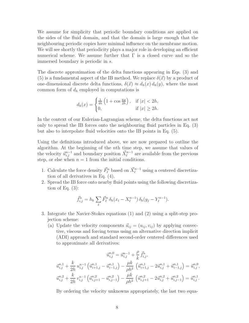
We assume for simplicity that periodic boundary conditions are applied onthe sides of the fluid domain, and that the domain is large enough that theneighbouring periodic copies have minimal influence on the membrane motion.We will see shortly that periodicity plays a major role in developing an efficientnumerical scheme. We assume further that Γ is a closed curve and so theimmersed boundary is periodic in s.

The discrete approximation of the delta functions appearing in Eqs. (3) and(5) is a fundamental aspect of the IB method. We replace δ(~x) by a product ofone-dimensional discrete delta functions, δ(~x) ≈ dh(x) dh(y), where the mostcommon form of dh employed in computations is

dh(x) =

14h

(1 + cos πx

2h

), if |x| < 2h,

0, if |x| ≥ 2h.

In the context of our Eulerian-Lagrangian scheme, the delta functions act notonly to spread the IB forces onto the neighbouring fluid particles in Eq. (3)but also to interpolate fluid velocities onto the IB points in Eq. (5).

Using the definitions introduced above, we are now prepared to outline thealgorithm. At the beginning of the nth time step, we assume that values ofthe velocity ~un−1

i,j and boundary position ~Xn−1ℓ are available from the previous

step, or else when n = 1 from the initial conditions.

1. Calculate the force density ~F nℓ based on ~Xn−1

ℓ using a centered discretiza-tion of all derivatives in Eq. (4).

2. Spread the IB force onto nearby fluid points using the following discretiza-tion of Eq. (3):

~fni,j = hb

∑

ℓ

~F nℓ δh(xi − Xn−1

ℓ ) δh(yj − Y n−1ℓ ).

3. Integrate the Navier-Stokes equations (1) and (2) using a split-step pro-jection scheme:(a) Update the velocity components ~uij = (uij, vij) by applying convec-

tive, viscous and forcing terms using an alternative direction implicit(ADI) approach and standard second-order centered differences usedto approximate all derivatives:

~un,0i,j = ~un−1

i,j +ρ

k~fni,j,

~un,1i,j +

k

2hun−1

i,j

(~un,1

i+1,j − ~un,1i−1,j

)− µk

ρh2

(~un,1

i+1,j − 2~un,1i,j + ~un,1

i−1,j

)= ~un,0

i,j ,

~un,2i,j +

k

2hvn−1

i,j

(~un,2

i,j+1 − ~un,2i,j−1

)− µk

ρh2

(~un,2

i,j+1 − 2~un,2i,j + ~un,2

i,j−1

)= ~un,1

i,j .

By ordering the velocity unknowns appropriately, the last two equa-

8

tions take the form of periodic tridiagonal systems and hence can besolved very efficiently.

(b) Project the velocity onto the space of divergence-free vector fields byfirst solving a Poisson equation for the pressure pn

i,j

pni+2,j + pn

i−2,j + pni,j+2 + pn

i,j−2 − 4pni,j =

2ρh

k

(un,2

i+1,j − un,2i−1,j + vn,2

i,j+1 − vn,2i,j−1

),

which is a 5-diagonal linear system that can be inverted efficientlyusing a Fast Fourier Transform because of the periodic boundaryconditions. The velocity is then updated via

~uni,j = ~un,2

i,j − k

2ρh

(pn

i+1,j − pni−1,j, pn

i,j+1 − pni,j−1

).

4. Evolve the boundary points in time using a forward Euler discretizationof Eq. (5),

~Xnℓ = ~Xn−1

ℓ +2αkhb

(~F n

ℓ · ~nn−1ℓ

)

| ~Xn−1ℓ+1 − ~Xn−1

ℓ−1 |+ kh2

∑

i,j

~uni,j δh(xi − Xn−1

ℓ ) δh(yj − Y n−1ℓ ).

5. Increment n and go to step 1.

The IB method as outlined above has a number of distinct advantages: itis efficient, having a computational cost of O(N2 log N) owing to the use ofthe FFT in the projection step; it is explicit in the sense that it is a step-by-step approach requiring no iteration; and it is simple to implement sinceno interpolation or complicated difference stencil corrections are needed atthe interface like in many other related methods for computing interfacialdynamics (i.e., the delta functions in the IB method handle the interpolationautomatically).

On the other hand, the IB method does have some disadvantages, the firstbeing that the centered treatment of convection terms limits the flows thatcan be handled to low Reynolds number (i.e., Re = 100 or less). Since the IBmethod was originally designed for simulating bio-fluid flow problems whereviscous effects typically dominate, this Re restriction is not a serious concernin some applications. The second major disadvantage is that the use of theapproximate delta function in combination with a discrete projection limits theaccuracy of the method to first order in space. One particular manifestationof this error is a violation of mass conservation which manifests itself as anon-physical slip velocity normal to the membrane – an issue that we treat inmore detail in the next section.

These drawbacks stem largely from the specific centered projection schemedescribed above, although there is nothing to prevent one from using anotherfluid solver that is more accurate and better suited to high-Re flows. Indeed,

9

several extensions to the IB method have been proposed in recent years thataddress the issues mentioned above, including high-order upwind discretiza-tions of the convection terms which allow simulation of convection-dominatedflows [17], and use of adaptive mesh refinement near the boundary to obtainsecond-order accuracy [12].

4 Volume Conservation

Before proceeding with the simulations, it is essential to first address the is-sue of errors in volume conservation in the IB method, since these errors canbe large enough to seriously pollute the numerical solution and preclude anymeaningful comparisons. The volume loss inherent in the IB method has beenrecognized for some time, and various approaches have been developed forcountering it. Peskin and Printz [25] proposed a modification to the standardcentered difference stencils for the gradient, divergence and Laplacian oper-ators which better approximate the divergence-free condition (we will referto this as the “PP method”). This modification typically reduces the volumeerror by at least one order of magnitude, but it comes at the expense of ap-proximately doubling the computational cost because of an increase in thedifference stencil widths.

Newren [21] observed that when the fluid velocity is interpolated onto IBpoints using the discrete version of Eq. (5), errors in volume conservation arisebecause the interpolated velocity does not identically satisfy the divergence-free constraint. He therefore proposed an alternate approach in which the IBvelocity is corrected in a post-processing step to ensure that the area containedwithin the membrane is conserved exactly. The method is simple and efficient,but works only for closed immersed boundaries in two dimensions.

Lee and LeVeque [19] developed a hybrid approach for simulating immersedboundaries, based on a combination of the immersed interface method andthe IB method, which uses a higher order correction to the difference sten-cils for the jump in normal stress across the membrane (i.e., correcting forthe pressure jump condition). An entirely different approach called the blobprojection method was developed by Cortez and Minion [8] and they includedetailed comparisons of their approach with the IB method, as well as exten-sive discussion of volume conservation.

We propose here an alternate strategy for dealing with volume loss that isinspired by a comment of Peskin and Printz [25], who observed in their com-putations that “volume conservation was not exact, and indeed that there wasa systematic tendency for a closed, pressurized chamber to lose volume slowlyat a rate proportional to the pressure difference across its walls, almost as if the

10

fluid were leaking out through a porous boundary.” They performed detailednumerical experiments with fluid marker particles to demonstrate that therewas no actual leakage of fluid through the immersed boundary. Nonetheless,there is a normal slip velocity which increases with the pressure drop, and soit seems reasonable to suggest that intrinsic volume loss in the IB method canbe represented in a manner analogous to flux through a porous membrane fluxby introducing an additional normal slip velocity of the form

Uv = −Kv [[p]]

µa= −Kv(~F · ~n)

µa | ~Xs|, (19)

where Kv (units of cm2) is the intrinsic permeability of the discretized im-mersed boundary. The IB method may then be corrected for volume conser-vation errors by simply adding a term Uv~n to the discrete version of Eq. (10).For a porous membrane, this is equivalent to replacing the membrane perme-ability K with the corrected value (K − Kv).

The membrane thickness a cannot be determined ahead of time since it isactually an effective thickness that derives from the smoothing radius of thediscrete delta function. Therefore, we choose a = 4h = 0.0625 for the pur-poses of specifying the analytical solution and use the corresponding effectivethickness a = Ca in computations, which is equivalent to replacing the porousslip parameter α with α = K/(Cµa). The actual value of the dimensionlessparameter C needs to be determined numerically, although we expect that awill be slightly less than the delta smoothing radius, meaning that C / 1.

The parameters Kv and C will depend on the discretization (namely, h and/orhb) and so both must be determined computationally for a given problem. Wepropose the following simple estimation procedure:

1. First perform a simulation with Req = 0 and K = 0, and a time intervalchosen long enough for the membrane to settle down to its linear rate ofdecay. The membrane velocity Uv is then approximated from the slopeof the r versus t curve, after which Eq. (19) yields an estimate for theintrinsic permeability,

Kv ≈ −(slope) µa | ~Xs|~F · ~n

.

2. Repeat the simulation from Step 1, taking some positive value of thepermeability K > 0 and the modified parameter α = K/(Cµa). Startingfrom an initial guess of C = 1, adjust C iteratively until the numericalsolution coincides with the analytical formula (16).

This is a straightforward procedure that can be easily automated and imple-mented as an initial calibration step in any immersed boundary code.

11

5 Numerical Simulations

In this section, we present results from a number of simple test cases to in-vestigate the effectiveness of the porous IB model as well as our new volumecorrection approach. In order to minimize the effects of intrinsic volume lossand focus instead on the physical porosity, we have chosen to implement thePeskin-Printz (PP) method which ensures that Kv ≪ K for the parameters ofinterest. Their approach is based on modifying the Fourier coefficients of boththe pressure solve and the discrete divergence stencil used in the projectionstep (we refer the reader to [25] for implementation details).

In all of the simulations to follow, we choose a square fluid domain with sidelength L = 1 cm and take fluid parameters ρ = 1 g/cm3 and µ = 1.0 g/cm s.Initially, we take σ = 105 g/cm s2 which is typical of other IB simulationsfor biological flows that have appeared in the literature. The fluid domainis discretized with N = 64 points in each direction and the membrane withNb = 200 points.

5.1 Circular Membrane: Correcting for Volume Loss

As a first computational test example, we consider a circular membrane withinitial radius Ro = 0.4 and equilibrium radius Req = 0, for which the analyticalsolution exhibits a linear decay to equilibrium. This problem is dominated byporous membrane transport since there are no membrane deformations or flownon-uniformities to drive the membrane away from its circular state; hence,this problem represents an ideal scenario for studying porous effects.

In order to determine the volume correction parameters Kv and C, we firstperform a simulation with K = 0 which yields an intrinsic permeability ofKv = 1.8× 10−11. A second run with K = 10−6 (holding all other parametersunchanged) yields the estimate C = 0.794, corresponding to a membrane withan effective thickness of 3.17h, which should be compared to the 4h supportof the delta function. It is worthwhile noting that the volume error arisingfrom Kv will remain small as long as Kv ≪ K, and so for any given immersedboundary calculation Kv will set a limit on the membrane permeabilities thatcan reasonably be simulated.

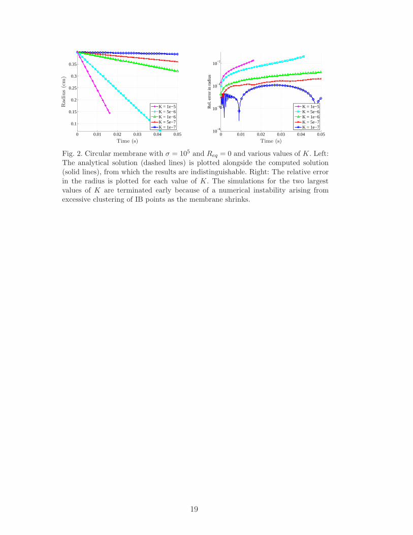
We then perform a series of simulations, holding Kv and C constant whileselecting permeabilities from the range K = [10−7, 10−5] in order to determinehow robust our proposed method is to changes in K. The plots of r(t) givenin Fig. 2 indicate that the computed and analytical solutions are nearly in-distinguishable from each other, and excellent agreement is obtained over theentire range of K considered. The errors increase as K increases which is to

12

be expected since a higher permeability will lead to larger porous flux, andwhen the velocity is large enough convective effects begin to play a significantrole. Recall that our analytical solution was derived based on the assumptionthat convection is negligible, which restricts its validity to small values of ασ.

[Fig. 2 about here.]

To test the robustness of our volume correction approach to changes in otherparameter values, we repeated the previous simulations but took instead asmaller value of the membrane stiffness, σ = 104. In this case, the IB forcedriving the motion is 10 times smaller and so the solution should exhibitsmaller fluid velocities and slower decay rate towards equilibrium. Fig. 3 con-tains the corresponding error plot for the radius. Keeping in mind that theerrors here accumulate over a time interval 10 times longer, we can concludethat the accuracy of our method remains comparable to that of the σ = 105

solution in Fig. 2.

[Fig. 3 about here.]

In order to compare our volume correction approach to other versions of theIB method, we simulate the case of σ = 105 and K = 10−6 using the originalIB approach and the uncorrected PP method. The error comparison in Fig. 4indicates that the PP approach is two orders of magnitude more accurate thanthe original IB method, which is consistent with other studies in the litera-ture [8,25]. When we incorporate our porous correction, the error is reducedby another factor of approximately three.

[Fig. 4 about here.]

Finally, we consider the more realistic situation where Req > 0 and the solutiondecays to steady state in a nonlinear fashion. Parameters are taken to be Req =0.2, σ = 105, and permeability is chosen from the range [10−5, 10−7] as before.The results depicted in Fig. 5 again show excellent agreement between theanalytical and numerical solutions. The analytical solution (which is includedin the plot of radius on the left) is indistinguishable from the computed results,and it is only in the error plot that the discrepancies are visible.

[Fig. 5 about here.]

5.2 Elliptical Membrane

Next, we consider a more interesting situation in which the membrane under-goes significant deformations and hence the membrane–fluid coupling playsan important role. To this end, we take the initial membrane to be an ellipse

13

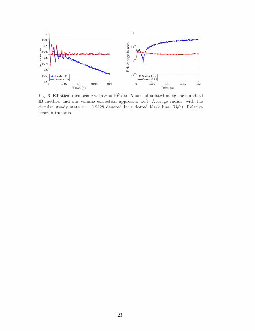
having semi-major and semi-minor axes rmax = 0.4, rmin = 0.2, and the un-stressed state is a circle of radius Req = 0.2 (this is a slightly modified versionof the test problem considered by LeVeque and Li [20]). The membrane os-cillates between horizontally- and vertically-elongated states, with the fluidviscosity gradually damping the motion and eventually settling down to a cir-cular steady state (look ahead to Fig. 8 for an illustration of the membranedynamics). In the non-porous case, the membrane should converge to a circleof radius

√rmin rmax = 0.2828, while for a porous membrane the steady state

circle has radius Req = 0.2.

A comparison of the computed results with and without volume is providedbyFig. 6 for σ = 105. The effectiveness of our approach is demonstrated bythe plots of average radius and relative error in the area, |A(t) − A(0)|/A(0),where A(t) represents the area enclosed by the membrane and A(0) is theexact (initial) value.

[Fig. 6 about here.]

To investigate the effect of changes in permeability on membrane motion, werepeat the last simulation for a selection of non-zero permeabilities and re-port the results in Fig. 7. Since the elliptical membrane decays to a circularshape over time, a meaningful comparison is still possible between the nu-merical solution for the elliptical membrane (in terms of average radius) andour analytical solution (16) for a circular membrane (with Ro = 0.2828 andReq = 0.2). The exact solution for each K is included in the plot of radiusin Fig. 7 using dashed lines, and once the initial oscillations of the ellipticmembrane die out, there is a very close correspondence with the analyticalsolution.

[Fig. 7 about here.]

The dynamics of the elliptical membrane are more clearly seen in Fig. 8 whichdepicts the membrane motion throughout the first period of oscillation. Theloss of volume owing to porous leakage is also evident from this plot.

[Fig. 8 about here.]

6 Conclusions

In this paper, we developed a simple approach for incorporating the effect ofmembrane porosity in the IB method in two dimensions, which requires theaddition of a porous slip velocity term to the boundary evolution equation.This modification is easily implemented in an existing IB code, and requires

14

virtually no additional cost since it involves quantities that are already com-puted. We also derived an explicit, radially-symmetric solution – valid forsmall values of the permeability K and small flow velocities – which may beused to validate porous IB simulations. The analytical and numerical solutionsare compared for a number of membrane geometries and physical parameters,and show very good agreement.

We also investigated the hypothesis that volume conservation errors inherentin the IB method can be attributed to an additional porous flux through theimmersed boundary. The rate of volume loss in any given IB computation isdependent on both the discretization and physical parameters, and can be fullycaptured by introducing two new parameters: an intrinsic permeability (Kv)and an effective membrane thickness (Ca). We presented a straightforwardprocedure for estimating Kv and C numerically, and showed that their valuesremain constant when certain problem parameters are varied. Therefore, ourapproach has the potential to be a general technique correcting volume errorsin the IB method.

Our treatment of volume conservation errors is by no means a comprehensivestudy and so further work is required to determine the sensitivity of Kv and Cto changes in parameters describing the fluid, membrane and discretization.In order to determine how useful our approach is in practice, more extensivesimulations are needed that consider not only a wider range of permeabilitiesrelevant to physical applications, but also more general IB configurations.

While our radially symmetric analytical solution is useful in validating com-putations, analysis of more general 2D membrane configurations would alsobe of interest. We therefore plan to extend the techniques developed in [28,9]to handle porous immersed boundaries. In future, we also intend to apply ournumerical method to the study of specific applications such as the propaga-tion of ocean waves through porous wave barriers, and pulsatile flow of bloodthrough arteries with porous walls. Direct comparisons to other more stan-dard numerical methods for fluid structure interaction such as [3] will alsobe undertaken, and benchmark problems such as those reported in [2] will beinstrumental in demonstrating the practical value of our approach.

Acknowledgements

This work was funded by grants from the Natural Sciences and Engineering Re-search Council of Canada and the MITACS Network of Centres of Excellence.JMS gratefully acknowledges the support of the Alexander von HumboldtFoundation and the Fraunhofer Institut Techno- und Wirtschaftsmathematikin Kaiserslautern, Germany.

15

References

[1] K. M. Arthurs, L. C. Moore, C. S. Peskin, E. B. Pitman, and H. E. Layton.Modeling arteriolar flow and mass transport using the immersed boundarymethod. J. Comput. Phys., 147:402–440, 1998.

[2] K.-J. Bathe and G. A. Ledezma. Benchmark problems for incompressible fluidflows with structural interactions. Computers & Structures, 85:628–644, 2007.

[3] K.-J. Bathe and H. Zhang. Finite element developments for general fluid flowswith structural interactions. Int. J. Numer. Meth. Eng., 60:213–232, 2004.

[4] J. Bear. Dynamics of Fluids in Porous Media. Dover, New York, 1988.

[5] A. T. Chwang. A porous-wavemaker theory. J. Fluid Mech., 132:395–406, 1983.

[6] R. M. Corless, G. H. Gonnet, D. E. G. Hare, D. J. Jeffrey, and D. E. Knuth.On the Lambert W function. Adv. Comput. Math., 5:329–359, 1996.

[7] R. Cortez, L. Fauci, N. Cowen, and R. Dillon. Simulations of swimmingorganisms: Coupling internal mechanics with external fluid dynamics. Comput.

Sci. & Eng., 6(3):38–45, May/June 2004.

[8] R. Cortez and M. Minion. The blob projection method for immersed boundaryproblems. J. Comput. Phys., 161(2):428–453, 2000.

[9] R. Cortez, C. S. Peskin, J. M. Stockie, and D. A. Varela. Parametric resonancein immersed elastic boundaries. SIAM J. Appl. Math., 65(2):494–520, 2004.

[10] R. Dillon and L. Fauci. Microscale model of bacterial and biofilm dynamics inporous media. Biotechnol. Bioeng., 68(5):536–547, 2000.

[11] R. Dillon, L. J. Fauci, A. L. Fogelson, and D. Gaver III. Modeling biofilmprocesses using the immersed boundary method. J. Comput. Phys., 129(1):57–73, 1996.

[12] B. E. Griffith, R. D. Hornung, D. M. McQueen, and C. S. Peskin. An adaptive,formally second order accurate version of the immersed boundary method. J.

Comput. Phys., 223(1):10–49, 2007.

[13] Z. J. Huang and J. M. Tarbell. Numerical simulation of mass transfer in porousmedia of blood vessel walls. Amer. J. Physiol. Heart Circ. Physiol., 273(1):464–477, 1997.

[14] J. T. Jenkins. Static equilibrium configurations of a model red blood cell. J.

Math. Biol., 4:149–169, 1977.

[15] M. H. Kim and S. T. Kee. Flexible-membrane wave barrier. I: Analytic andnumerical solutions. J. Waterway, Port, Coastal, Ocean Eng., 122(1):46–53,1996.

[16] Y. Kim and C. S. Peskin. 2-D parachute simulation by the immersed boundarymethod. SIAM J. Sci. Comput., 28(6):2294–2312, 2006.

16

[17] M. C. Lai and C. S. Peskin. An immersed boundary method with formal second-order accuracy and reduced numerical viscosity. J. Comput. Phys., 160(2):705–719, 2000.

[18] A. T. Layton. Modeling water transport across elastic boundaries using anexplicit jump method. SIAM J. Sci. Comput., 28(6):2189–2207, 2006.

[19] L. Lee and R. J. LeVeque. An immersed interface method for incompressibleNavier-Stokes equations. SIAM J. Sci. Comput., 25(3):832–856, 2003.

[20] R. J. LeVeque and Z. Li. Immersed interface methods for Stokes flow withelastic boundaries or surface tension. SIAM J. Sci. Comput., 18(3):709–735,1997.

[21] E. P. Newren. Enhancing the immersed boundary method: Stability, volume

conservation, and implicit solvers. PhD thesis, University of Utah, Salt LakeCity, UT, 2007.

[22] C. S. Peskin. Numerical analysis of blood flow in the heart. J. Comput. Phys.,25:220–252, 1977.

[23] C. S. Peskin. The immersed boundary method. In Acta Numerica, volume 11,pages 1–39. Cambridge University Press, 2002.

[24] C. S. Peskin and D. M. McQueen. A three-dimensional computational modelfor blood flow in the heart. I. Immersed elastic fibers in a viscous incompressiblefluid. J. Comput. Phys., 81:372–405, 1989.

[25] C. S. Peskin and B. F. Printz. Improved volume conservation in the computationof flows with immersed elastic boundaries. J. Comput. Phys., 105:33–46, 1993.

[26] S. Sivaloganathan, M. Stastna, G. Tenti, and J. M. Drake. Biomechanics of thebrain: A theoretical and numerical study of biot’s equations of consolidationtheory with deformation-dependent permeability. Int. J. Nonlin. Mech.,40(9):1149–1159, 2005.

[27] J. M. Stockie and S. I. Green. Simulating the motion of pulp fibres using theimmersed boundary method. J. Comput. Phys., 147(1):147–165, 1998.

[28] J. M. Stockie and B. T. R. Wetton. Stability analysis for the immersed fiberproblem. SIAM J. Appl. Math., 55(6):1577–1591, 1995.

17

0 0.1 0.2 0.3 0.4 0.50

0.05

0.1

0.15

0.2

0.25

0.3

0.35

0.4

Time (s)

Radiu

s(c

m)

Req = 0

Req = 0.2

Fig. 1. The analytical solution for a circular membrane is displayed for ασ = 0.016,equilibrium radii Req = 0 and 0.2, and initial radii Ro = 0.1, 0.3 and 0.4. Theintercepts t = Ro/ασ for the Req = 0 solution are depicted on the t–axis using opencircles.

18

0 0.01 0.02 0.03 0.04 0.05

0.1

0.15

0.2

0.25

0.3

0.35

K = 1e−5K = 5e−6K = 1e−6K = 5e−7K = 1e−7

Time (s)

Radiu

s(c

m)

0 0.01 0.02 0.03 0.04 0.0510

−8

10−6

10−4

10−2

Rel

. err

or in

rad

ius

K = 1e−5K = 5e−6K = 1e−6K = 5e−7K = 1e−7

Time (s)

Fig. 2. Circular membrane with σ = 105 and Req = 0 and various values of K. Left:The analytical solution (dashed lines) is plotted alongside the computed solution(solid lines), from which the results are indistinguishable. Right: The relative errorin the radius is plotted for each value of K. The simulations for the two largestvalues of K are terminated early because of a numerical instability arising fromexcessive clustering of IB points as the membrane shrinks.

19

0 0.1 0.2 0.3 0.4 0.5

10−6

10−4

10−2

Rel

. err

or in

rad

ius

K = 1e−5K = 5e−6K = 1e−6K = 5e−7K = 1e−7

Time (s)

Fig. 3. Circular membrane with σ = 104 and Req = 0. The relative error in themembrane radius is plotted for the same values of K as in Fig. 2.

20

0.01 0.02 0.03 0.04 0.0510

−6

10−4

10−2

100

Standard IBPeskin−PrintzCorrected PP

Time (s)R

el.er

ror

inra

diu

s

Fig. 4. Plots of solution error for the circular membrane with σ = 105, Req = 0, andK = 10−6, using three different methods for correcting volume loss: the standardIB method, and the PP volume-conserving stencil with Kv = 0 and 1.8 × 10−11.

21

0 0.1 0.2 0.3 0.4 0.50.2

0.25

0.3

0.35

K = 1e−5K = 5e−6K = 1e−6K = 5e−7K = 1e−7

Time (s)

Radiu

s(c

m)

0 0.1 0.2 0.3 0.4 0.510

−8

10−6

10−4

10−2

Rel

. err

or in

rad

ius

K = 1e−5K = 5e−6K = 1e−6K = 5e−7K = 1e−7

Time (s)

Fig. 5. Plots of the radius (left) and error (right) for the circular membrane withσ = 105, Req = 0.2, and various values of K.

22

0 0.005 0.01 0.015 0.020.26

0.265

0.27

0.275

0.28

0.285

0.29

0.295

0.3

Avg

. rad

ius

(cm

)

Standard IBCorrected PP

Time (s)

0 0.005 0.01 0.015 0.02

10−6

10−4

10−2

100

Standard IBCorrected PP

Time (s)

Rel

.ch

ange

inare

a

Fig. 6. Elliptical membrane with σ = 105 and K = 0, simulated using the standardIB method and our volume correction approach. Left: Average radius, with thecircular steady state r = 0.2828 denoted by a dotted black line. Right: Relativeerror in the area.

23

0 0.002 0.004 0.006 0.008 0.010.2

0.22

0.24

0.26

0.28A

vg. r

adiu

s (c

m)

K = 0K = 1e−6K = 1e−5K = 2e−5

Time (s)

0 0.002 0.004 0.006 0.008 0.0110

−8

10−6

10−4

10−2

100

K = 0K = 1e−6K = 1e−5K = 2e−5

Time (s)

Rel

.ch

ange

inare

a

Fig. 7. Elliptical membrane with σ = 105 and various values of the permeability.Left: Average radius, with the corresponding circular exact solutions plotted usingdashed lines. Right: Relative change in radius, |A − A(0)|/A(0).

24

t = 0.0 t = 0.0006 t = 0.0012

0 0.2 0.4 0.6 0.8 10

0.2

0.4

0.6

0.8

1

K = 0K = 1e−6K = 1e−5K = 2e−5

x (cm)

y(c

m)

0 0.2 0.4 0.6 0.8 10

0.2

0.4

0.6

0.8

1

K = 0K = 1e−6K = 1e−5K = 2e−5

x (cm)

y(c

m)

0 0.2 0.4 0.6 0.8 10

0.2

0.4

0.6

0.8

1

K = 0K = 1e−6K = 1e−5K = 2e−5

x (cm)

y(c

m)

t = 0.0018 t = 0.0024 t = 0.0030

0 0.2 0.4 0.6 0.8 10

0.2

0.4

0.6

0.8

1

K = 0K = 1e−6K = 1e−5K = 2e−5

x (cm)

y(c

m)

0 0.2 0.4 0.6 0.8 10

0.2

0.4

0.6

0.8

1

K = 0K = 1e−6K = 1e−5K = 2e−5

x (cm)

y(c

m)

0 0.2 0.4 0.6 0.8 10

0.2

0.4

0.6

0.8

1

K = 0K = 1e−6K = 1e−5K = 2e−5

x (cm)

y(c

m)

Fig. 8. Time evolution of an elliptical membrane with σ = 105 and various valuesof K.

25