UNIVERSITY OF SOUTHAMPTON

Faculty of Natural and Environmental SciencesOcean and Earth Science

National Oceanography Centre, University of Southampton

WAVE DISSIPATION PATTERNSAS AN INDICATOR OFRIP CURRENT HAZARD

By

SEBASTIAN JOHN PITMAN

Thesis for the degree of Doctor of Philosophy

March 2017

UNIVERSITY OF SOUTHAMPTON

ABSTRACT

FACULTY OF NATURAL AND ENVIRONMENTAL SCIENCES

Ocean and Earth Sciences

Doctor of Philosophy

WAVE DISSIPATION PATTERNS AS AN INDICATOR OF RIPCURRENT HAZARDby Sebastian John Pitman

Rip currents (rips) are hazardous offshore-directed flows in the surfzone of beaches worldwide.Rips are a major hazard for recreational beach use and are the dominant cause of beachrescues and drownings. It is therefore important to understand what conditions make a ripmost hazardous, in order for beach safety practitioners to mitigate the risk. The aim ofthis thesis was to determine how patterns of wave breaking influence rip channel hazard onbeaches. In order to quantify wave breaking, video imagery from three hydrodynamicallydiverse case studies was used, and validated at two sites against Lagrangian GPS drifterdata. This thesis first developed pre-processing techniques for video imagery which thensubsequently improved the reliability of rip channel detection. Hitherto, the noise inherentin such signals has made automated detection of rip currents problematic. Wave breakingpatterns could then be identified with the novel application of synoptic typing methods tothe imagery, resulting in a classification scheme for rip currents based on wave breaking.Two dominant types were identified: (1) open channels, whereby the rip channel hasfree connectivity to the region beyond the surfzone; and (2) closed channels, where wavebreaking across the seaward extent of the channel effectively closes this connectivity to theoffshore region. Investigation of Lagrangian data for each of the prevailing states showsthat under open conditions, drifters were highly likely to be transported beyond the edgeof the surfzone by the rip current, with exit rates reaching 100 % at times. Under closedconditions, drifters were more likely to be retained in the surfzone, with typical exit ratesbetween 0 and 35 %. A rip current that exits the surfzone is more hazardous to bathers,and therefore, this thesis subsequently investigated the prevalence of open and closed ripchannels in records of rip rescue events. Over two sites for which data were available,upwards of two thirds of major rip rescues occurred when the channel could be classifiedby this new method as open. Furthermore, the majority of surfer and bodyboarder rescuesoccurred under open conditions. Despite their over-representation in the rip rescue record,the overall prevalence of open channels over a year is only around 40 %. Normalising thenumber of rescues in open rips by their occurrence shows open rips to be twice as hazardousas closed channels. This new approach provides a quick and inexpensive means to assesshigh risk surf conditions at rip beaches worldwide, with the deployment of only a small(often mobile) imaging system.

Contents

Table of contents . . . . . . . . . . . . . . . . . . . . . . . . . . . . . . . . . . . iList of figures . . . . . . . . . . . . . . . . . . . . . . . . . . . . . . . . . . . . . vList of tables . . . . . . . . . . . . . . . . . . . . . . . . . . . . . . . . . . . . . xvDeclaration of authorship . . . . . . . . . . . . . . . . . . . . . . . . . . . . . . xviiAcknowledgements . . . . . . . . . . . . . . . . . . . . . . . . . . . . . . . . . . xixDefinitions and abbreviations . . . . . . . . . . . . . . . . . . . . . . . . . . . . xx

1 Introduction 11.1 Background . . . . . . . . . . . . . . . . . . . . . . . . . . . . . . . . . . . 11.2 Aims and objectives . . . . . . . . . . . . . . . . . . . . . . . . . . . . . . 61.3 Thesis structure . . . . . . . . . . . . . . . . . . . . . . . . . . . . . . . . . 8

2 Literature review 92.1 Automated detection of rip currents . . . . . . . . . . . . . . . . . . . . . . 9

2.1.1 Video remote sensing . . . . . . . . . . . . . . . . . . . . . . . . . . 102.1.2 Quantitative use of video imagery . . . . . . . . . . . . . . . . . . . 122.1.3 Attempts to automate rip detection . . . . . . . . . . . . . . . . . . 152.1.4 Constraints and possible solutions . . . . . . . . . . . . . . . . . . . 17

2.2 Rip channel classification . . . . . . . . . . . . . . . . . . . . . . . . . . . . 192.2.1 Objective surfzone classification . . . . . . . . . . . . . . . . . . . . 192.2.2 Rip current classification . . . . . . . . . . . . . . . . . . . . . . . . 222.2.3 The effect and quantification of rip channel shape . . . . . . . . . . 24

2.3 Controls on surfzone retention . . . . . . . . . . . . . . . . . . . . . . . . . 262.3.1 Rip current circulation . . . . . . . . . . . . . . . . . . . . . . . . . 262.3.2 Controls on circulation . . . . . . . . . . . . . . . . . . . . . . . . . 262.3.3 Retention rates . . . . . . . . . . . . . . . . . . . . . . . . . . . . . 282.3.4 Wave breaking patterns as a control on retention . . . . . . . . . . 29

2.4 Control on rip current hazard . . . . . . . . . . . . . . . . . . . . . . . . . 322.4.1 Coastal drownings . . . . . . . . . . . . . . . . . . . . . . . . . . . 32

i

2.4.2 Hazard and risk . . . . . . . . . . . . . . . . . . . . . . . . . . . . . 332.4.3 Escape strategies . . . . . . . . . . . . . . . . . . . . . . . . . . . . 33

2.5 Summary & knowledge gaps . . . . . . . . . . . . . . . . . . . . . . . . . . 36

3 Study sites 393.1 Tairua Beach, Coromandel, New Zealand . . . . . . . . . . . . . . . . . . . 393.2 Perranporth Beach, Devon, U.K. . . . . . . . . . . . . . . . . . . . . . . . 413.3 Ngarunui Beach, Raglan, New Zealand . . . . . . . . . . . . . . . . . . . . 43

4 Data & methods 474.1 Data . . . . . . . . . . . . . . . . . . . . . . . . . . . . . . . . . . . . . . . 47

4.1.1 Lagrangian rip current data . . . . . . . . . . . . . . . . . . . . . . 474.1.2 Hydrodynamics and bathymetry . . . . . . . . . . . . . . . . . . . . 534.1.3 Video imagery . . . . . . . . . . . . . . . . . . . . . . . . . . . . . . 564.1.4 Rip incident data . . . . . . . . . . . . . . . . . . . . . . . . . . . . 59

4.2 Methods . . . . . . . . . . . . . . . . . . . . . . . . . . . . . . . . . . . . . 604.2.1 Drifter GPS data . . . . . . . . . . . . . . . . . . . . . . . . . . . . 604.2.2 Bathymetry . . . . . . . . . . . . . . . . . . . . . . . . . . . . . . . 634.2.3 Video imagery . . . . . . . . . . . . . . . . . . . . . . . . . . . . . . 63

5 Synthetic imagery for rip channel detection 655.1 Introduction . . . . . . . . . . . . . . . . . . . . . . . . . . . . . . . . . . . 655.2 Methodology . . . . . . . . . . . . . . . . . . . . . . . . . . . . . . . . . . 67

5.2.1 Image rectification . . . . . . . . . . . . . . . . . . . . . . . . . . . 675.2.2 Image filtering . . . . . . . . . . . . . . . . . . . . . . . . . . . . . . 685.2.3 Shoreline detection . . . . . . . . . . . . . . . . . . . . . . . . . . . 715.2.4 Barline position . . . . . . . . . . . . . . . . . . . . . . . . . . . . . 715.2.5 Creation of a synthetic image . . . . . . . . . . . . . . . . . . . . . 755.2.6 Minima detection . . . . . . . . . . . . . . . . . . . . . . . . . . . . 765.2.7 Rip grouping . . . . . . . . . . . . . . . . . . . . . . . . . . . . . . 795.2.8 Application of method . . . . . . . . . . . . . . . . . . . . . . . . . 79

5.3 Results . . . . . . . . . . . . . . . . . . . . . . . . . . . . . . . . . . . . . . 805.3.1 Automation of rip detection . . . . . . . . . . . . . . . . . . . . . . 805.3.2 Utility of synthetic imagery for rip detection . . . . . . . . . . . . . 84

5.4 Discussion . . . . . . . . . . . . . . . . . . . . . . . . . . . . . . . . . . . . 865.4.1 Progress in automated detection . . . . . . . . . . . . . . . . . . . . 865.4.2 Value of filtering and synthetic imagery . . . . . . . . . . . . . . . . 895.4.3 Thresholding imagery . . . . . . . . . . . . . . . . . . . . . . . . . . 90

5.5 Conclusions . . . . . . . . . . . . . . . . . . . . . . . . . . . . . . . . . . . 91

ii

6 Classification of rip channel morphologies 936.1 Introduction . . . . . . . . . . . . . . . . . . . . . . . . . . . . . . . . . . . 936.2 Methodology . . . . . . . . . . . . . . . . . . . . . . . . . . . . . . . . . . 946.3 Results . . . . . . . . . . . . . . . . . . . . . . . . . . . . . . . . . . . . . . 99

6.3.1 Synoptic typing . . . . . . . . . . . . . . . . . . . . . . . . . . . . . 996.3.2 Hydrodynamic controls . . . . . . . . . . . . . . . . . . . . . . . . . 1026.3.3 Temporal controls . . . . . . . . . . . . . . . . . . . . . . . . . . . . 110

6.4 Discussion . . . . . . . . . . . . . . . . . . . . . . . . . . . . . . . . . . . . 1116.4.1 Synoptic typing of surfzone imagery . . . . . . . . . . . . . . . . . . 1116.4.2 Classification and hydrodynamic control . . . . . . . . . . . . . . . 1126.4.3 Temporal controls . . . . . . . . . . . . . . . . . . . . . . . . . . . . 117

6.5 Conclusions . . . . . . . . . . . . . . . . . . . . . . . . . . . . . . . . . . . 118

7 Wave dissipation as an indicator of nearshore circulation 1217.1 Introduction . . . . . . . . . . . . . . . . . . . . . . . . . . . . . . . . . . . 1217.2 Methodology . . . . . . . . . . . . . . . . . . . . . . . . . . . . . . . . . . 122

7.2.1 Video imagery . . . . . . . . . . . . . . . . . . . . . . . . . . . . . . 1237.2.2 Lagrangian drifter data . . . . . . . . . . . . . . . . . . . . . . . . . 123

7.3 Results . . . . . . . . . . . . . . . . . . . . . . . . . . . . . . . . . . . . . . 1267.3.1 Hydrodynamics . . . . . . . . . . . . . . . . . . . . . . . . . . . . . 1267.3.2 Wave breaking controls . . . . . . . . . . . . . . . . . . . . . . . . . 133

7.4 Discussion . . . . . . . . . . . . . . . . . . . . . . . . . . . . . . . . . . . . 1397.5 Conclusions . . . . . . . . . . . . . . . . . . . . . . . . . . . . . . . . . . . 145

8 Quantifying rip current hazard 1478.1 Introduction . . . . . . . . . . . . . . . . . . . . . . . . . . . . . . . . . . . 1478.2 Methodology . . . . . . . . . . . . . . . . . . . . . . . . . . . . . . . . . . 149

8.2.1 Rip incident data . . . . . . . . . . . . . . . . . . . . . . . . . . . . 1498.2.2 Hydrodynamic analysis . . . . . . . . . . . . . . . . . . . . . . . . . 151

8.3 Results . . . . . . . . . . . . . . . . . . . . . . . . . . . . . . . . . . . . . . 1518.3.1 Demographics . . . . . . . . . . . . . . . . . . . . . . . . . . . . . . 1528.3.2 Hindcast hydrodynamics - Ngarunui . . . . . . . . . . . . . . . . . 1528.3.3 Wave breaking patterns . . . . . . . . . . . . . . . . . . . . . . . . 157

8.4 Discussion . . . . . . . . . . . . . . . . . . . . . . . . . . . . . . . . . . . . 1608.4.1 Demographics - Ngarunui . . . . . . . . . . . . . . . . . . . . . . . 1608.4.2 Hydrodynamics - Ngarunui . . . . . . . . . . . . . . . . . . . . . . . 1608.4.3 Wave breaking patterns: Open vs. closed rips . . . . . . . . . . . . 163

8.5 Conclusions . . . . . . . . . . . . . . . . . . . . . . . . . . . . . . . . . . . 165

iii

9 Conclusions and implications 1679.1 Automation of rip detection & the use of synthetics . . . . . . . . . . . . . 1689.2 Morphological classification of rip currents . . . . . . . . . . . . . . . . . . 1699.3 Wave dissipation as a control on surfzone retention . . . . . . . . . . . . . 1719.4 Rip current hazard signature . . . . . . . . . . . . . . . . . . . . . . . . . . 1729.5 Summary . . . . . . . . . . . . . . . . . . . . . . . . . . . . . . . . . . . . 1739.6 Outlook for further work . . . . . . . . . . . . . . . . . . . . . . . . . . . . 177

Appendices 181Appendix A: GPS drifter data processing steps . . . . . . . . . . . . . . . . . . 182Appendix B: Rip perception paper . . . . . . . . . . . . . . . . . . . . . . . . . 186Appendix C: Rip current observations paper . . . . . . . . . . . . . . . . . . . . 193Appendix D: Pulsations in surfzone currents paper . . . . . . . . . . . . . . . . 197

iv

List of Figures

1.1 A schematic of a generalised rip current and associated nearshore circulations.Adapted from MacMahan et al. (2006) and based on early observations. . 3

1.2 (a) A mass rescue from a rip current at Busan beach, South Korea, and (b)the aftermath of the rescue whereby lifeguards have cleared the area of thebeach associated with the rip current. Photo credit: J. Lee. . . . . . . . . . 4

2.1 The three-camera monitoring system installed at Droskyn Point to monitorPerranporth. Picture taken at high tide, with cameras orientated to capturelow tide intertidal beach area. Photo credit: S Pitman. . . . . . . . . . . . 11

2.2 Examples of (a) snapshot, (b) timex, and (c) variance images collected bythe Argus camera at Droskyn Point on 25 Jul 2013. . . . . . . . . . . . . . 13

2.3 An example of a rectified and merged image from the Droskyn Point camera,Perranporth, with prominent features labelled. The black corners are areasoutside the field of view of the camera. A seam is visible running alongshorenear the waters edge, where images from two different fields of view havebeen merged together. . . . . . . . . . . . . . . . . . . . . . . . . . . . . . 14

2.4 Example use of temporary GCPs (when no permanent features are visible inthe image) at Perranporth, U.K. This image depicts checker boards placedon the beach (black circles), providing easily identifiable static positions inthe image. Additionally, the static RNLI truck has also been used as anextra GCP. Photo extract from Argus archive. . . . . . . . . . . . . . . . . 16

2.5 Wright and Short (1984) beach state classification scheme. Illustration fromRanasinghe et al. (2004). . . . . . . . . . . . . . . . . . . . . . . . . . . . . 21

2.6 Contemporary view of rip current circulation, indicating the propensity forrecirculatory flow, in addition to exits. Following the work of Austin et al.(2010) and MacMahan et al. (2010). . . . . . . . . . . . . . . . . . . . . . . 27

v

2.7 Conceptual representation of rip behaviour as a function of wave and tidalcontrols. LW refers to the height of the corresponding low water as anabsolute water depth (m above CD). The overbar is indicative of the longterm mean values. Large positive values of tide factor are indicative ofneap tide conditions and large negative values indicative of spring tides.HT refers to significant wave height × peak period, with the again overbarindicative of long term mean values. Taken from Scott et al. (2014). . . . . 28

3.1 Map of Tairua Beach, New Zealand, with the field study location enclosedby a black box. The Cam-Era camera station is located on cliffs to thesouth (black circle). . . . . . . . . . . . . . . . . . . . . . . . . . . . . . . . 40

3.2 Image of Tairua Beach. Photo credit: backpack-newzealand.com. . . . . . 403.3 Map of Perranporth, U.K., with the field study location enclosed by a black

box. The black circle shows the position of the Argus camera station, andthe star the directional Waverider wave buoy. . . . . . . . . . . . . . . . . 43

3.4 Image of Perranporth Beach, with multiple clearly identifiable rip channelsalongshore [dark, shore-normal streaks intersecting the breaking waves].Photo credit: S. Pitman. . . . . . . . . . . . . . . . . . . . . . . . . . . . 44

3.5 Map of Ngarunui Beach, New Zealand, with the field study location enclosedby a black box. The black circle shows the position of the Cam-era videomonitoring station. . . . . . . . . . . . . . . . . . . . . . . . . . . . . . . 46

3.6 Image of Ngarunui Beach. Photo credit: aa.co.nz. . . . . . . . . . . . . . 46

4.1 Photograph of the GPS drifters during fieldwork at Perranporth. Withoutballast, the drifters stand 1200 mm in height. The design is modified fromSchmidt et al. (2003) and MacMahan et al. (2009). Photo credit: S. Pitman. 49

4.2 Photograph of the GPS drifters during fieldwork at Ngarunui. Photo credit:S. Gallop. . . . . . . . . . . . . . . . . . . . . . . . . . . . . . . . . . . . . 52

4.3 Summary of field conditions from 16 to 20 May 2014 at Perranporth Beach,with vertical grey bars indicating drifter deployments: a) water level Htide;b) significant wave height Hs; c) peak wave period Tp; d) incident wavedirection θ; e) wind speed U ; and f) wind direction WDir. Red lines indicatethe shore-normal direction. ODN refers to Ordnance Datum Newlyn, whichis approximate Mean Sea Level in the UK. . . . . . . . . . . . . . . . . . . 54

4.4 Bathymetry and drifter data for the field experiment with white boxesindicative of study area and solid black line is 0 m ODN. (a) The mergedbathymetric and topographic data, measured on 17 May 2014. (b) Theresidual morphology. (c) The overlay of merged, rectified images from theArgus camera onto the bathymetry. . . . . . . . . . . . . . . . . . . . . . . 55

vi

4.5 Summary of field conditions from 8 to 13 Feb 2015 at Ngarunui Beach,with vertical grey bars indicating drifter deployments: a) water level Htide;b) significant wave height Hs; c) peak wave period Tp; d) incident wavedirection θ; e) wind speed U ; and f) wind direction WDir. Red lines indicatethe shore-normal direction. Tidal heights are reference to MSL. . . . . . . 57

4.6 Bathymetry data for Ngarunui. The solid black line represents MSL. (a)The general bathymetric data merged with topographic data measured on 8Feb 2015. (b) The residual morphology. (c) The overlay of merged, rectifiedimages from the Cam-Era station onto the residual morphology. . . . . . . 58

4.7 Bathymetry and drifter data for the Perranporth field experiment withwhite boxes indicative of study area and solid black line is 0 m ODN. (a)Number of independent observations recorded at 0.1 Hz over the studyperiod, binned into 10 × 10 m grid squares. Grid squares with < 5observations appear as grey and are not considered further in the thesis. (b)Mean drifter velocities recorded during the experiment. (c) Overall surfzonevorticity over the experiment, with red values indicative of an anti-clockwisehorizontal rotation, and blue values indicative of clockwise rotation. . . . . 61

4.8 Bathymetry and drifter data for the Ngarunui field experiment with solidblack line is MSL. (a) Number of independent observations recorded at 0.1Hz over the study period, binned into 10 × 10 m grid squares. Grid squareswith < 5 observations appear as grey and are not considered further inthe thesis. (b) Mean drifter velocities recorded during the experiment. (c)Overall surfzone vorticity over the experiment, with red values indicative ofan anti-clockwise horizontal rotation, and blue values indicative of clockwiserotation. . . . . . . . . . . . . . . . . . . . . . . . . . . . . . . . . . . . . . 62

5.1 (a) Rectified timex image of Tairua Beach, New Zealand. Rain drop foulingis evident in the region of the blue transect line. (b) Filtered version of (a)with red transect line. (c) Intensity profiles for both transect lines, with themaxima marked by horizontal lines. (d) Onset of wave breaking detectedalongshore using intensity maxima transects, as per (c). . . . . . . . . . . . 70

5.2 (a) Original rectified timex image from Tairua Beach, New Zealand (NIWA).The image is orientated so that shoreline runs along the x-axis. (b) Theimage is first segregated into three groups, corresponding to the dominantred, green, and blue pixel clusters. The boundary between beach andbreaking zone is depicted well by this method, and is therefore used (c) asan approximation of shoreline. (d) The image is then converted to grayscalefor further processing. . . . . . . . . . . . . . . . . . . . . . . . . . . . . . 72

vii

5.3 (a) Derivation of barline for one individual column of pixels. The pixelsare shown in the bar below the figure, with the respective normalised pixelintensity along that bar shown above by the blue line. The 0.2 thresholdis marked (dashed line) and the first peak in intensity above that threshold(red line) is stored as the barline location. (b) Repetition of this methodfor every column of pixels in the image gives an estimate of the longshorevariable barline. . . . . . . . . . . . . . . . . . . . . . . . . . . . . . . . . . 74

5.4 Scatter intensity plot of algorithm and (a) manually derived shoreline and(b) barline locations, with white line representing 1:1 correlation. Thecolour is indicative of the number of observations at that location. . . . . . 75

5.5 (a) An original rectified image from Tairua Beach. (b) The parent image(a) was segmented into the offshore region, the beach, and then within thesurfzone into areas of wave breaking, and deeper channeled areas. (c—e)The pixel values from the original image (a) for each zone identified in(b) have been extracted, and presented in terms of their red, green, andblue pixel values. The zones in (b) are then filled with pixels randomlyselected from the corresponding pixel value distribution curve in (c—f).The resulting image is the synthetic image, with each zone now exhibitingthe dominant colour trend observed in the parent image. . . . . . . . . . . 77

5.6 (a) The detected barline and shoreline are used to create a masked image,depicting only the surfzone. The image has also been lowpass filtered. (b)The remaining image is thresholded so that areas of wave breaking (blacksection) can be removed from the search area. (c) Minima are then locatedin the remaining areas. Red lines depict the shore- and bar-line, with bluelines highlighting the search areas. Detected minima are shown as whitelines. (d) This search returns the minima contained within the darker partsof the image. (e) Significant features detected in the algorithm are storedas coherent rip currents (red features). . . . . . . . . . . . . . . . . . . . . 78

5.7 Test automated detections from Tairua Beach. The left column showsexpert digitisations, and provide the standard against which the automateddetections should be judged. The middle column shows detections madeon the original imagery. The right column shows detections made on thesynthetic imagery. Each row (a—d) shows images from a different time. . . 81

5.8 Test automated detections from Perranporth Beach. The left column showsexpert digitisations, and provide the standard against which the automateddetections should be judged. The middle column shows detections madeon the original imagery. The right column shows detections made on thesynthetic imagery. Each row (a—d) shows images from a different time.. . 82

viii

5.9 Sensitivity analysis of surfzone thresholding intensities. Left column showsthe original Perranporth image, and an annotation of the threshold used forsubsequent analysis. Middle column shows detected bar and shorelines (redlines), as well as the masking applied after the various intensity thresholdshave been applied to the surfzone. White lines are indicative of localminima detected. Right hand column shows the resulting rips detectedin the imagery. Each row (a—e) shows an image from a different time. . . 85

5.10 The user-digitized number of rips in each image obtained by digitizationcompared to the error in the number of rips detected in (a) the correspondingoriginal image and (b) synthetic image. Positive and negative numbersrepresent over- and under-predictions, respectively. Each prediction is representedas a scatter point. The data is binned by the user-digitized number of rips,with the mean (red line), the 1.96 standard error of the mean for each class(red bar), and the standard deviation (blue bar). . . . . . . . . . . . . . . . 86

5.11 Adaptation of the process used to create a synthetic image. (a) The original,rectified image, with a rip channel of interest manually selected (red box).(b) After thresholding, information about the pattern of wave breakingis evident, with white areas indicative of wave breaking and black areasindicative of the offshore or rip channel. . . . . . . . . . . . . . . . . . . . . 91

6.1 The original grayscale images (a and b), and the corresponding black andwhite images (c and d). These are two images that the Kirchofer analysisdeems similar. The overall difference (S) is shown with black indicativeof areas that are the same and white indicative of difference (f). Rowscores (SR) and column scores (SC) are shown as a blue line (e and g,respectively), the solid red line indicates the median score threshold appliedhere, and the dashed orange line shows the scores achieved. . . . . . . . . 97

6.2 Two rip channels extracted from the dataset (a and b) that the Kirchoferanalysis deems different. (d) The overall difference (S) is shown with blackindicative of areas that are the same and white indicative of difference. (c)Row scores (SR) and (e) column scores (SC) are shown as a blue line, thesolid red line indicates the median score threshold applied here, and thedashed orange line shows the scores achieved. . . . . . . . . . . . . . . . . 98

6.3 The four dominant rip channel configurations at Perranporth, classifiedusing synoptic typing. Black is indicative of rip channels and the offshoreregion, white depicts wave breaking over sand bars or subaerial beach. . . . 101

6.4 The four dominant rip channel keygrids (a—d) at Perranporth, and aselection of imagery from the database considered to be similar to the keygrids.102

ix

6.5 A compartmentalisation of the dataset based on wave and tide factors. Allimages within the requisite wave and tide conditions have been averaged,and then thresholded to form a black and white representation. . . . . . . 103

6.6 A compartmentalisation of the dataset based on wave and tide factors.Here, all variation from the averaging process was presented to reconstructexemplar greyscale imagery. . . . . . . . . . . . . . . . . . . . . . . . . . . 104

6.7 Standard deviations (σ) in compartmentalised imagery. . . . . . . . . . . . 1056.8 Standard deviations (σ) in the top Kirchofer group for each wave/tide

threshold. . . . . . . . . . . . . . . . . . . . . . . . . . . . . . . . . . . . . 1076.9 Distribution of (a) wave factor and (b) tide factor data points for each of

the four synoptic channel types. Red bars are indicative of median values,and notches show the 95 % confidence interval of the mean. . . . . . . . . . 108

6.10 Rip channel types as a function of wave and tide factors. For each quadrantof the wave-tide factor grid, the prevalence of each of the four channel typesis shown by the barcharts. The direction of transitions observed at each ofthe wave/tide conditions is shown by the arrows, with a transition beingdefined as the difference in synoptic type between one image and the nextone sampled at that same location (which may in fact be no change). . . . 109

6.11 Conceptualisation of different rip channel types. First order classificationis determined by whether the channel is deemed ‘open’ or ‘closed’ to theoffshore region. Second order exemplar channels for each type are shown. . 114

7.1 Examples of rip currents from Perranporth Beach, U.K. The examples hereare classified as (a) open; and (b) closed to the offshore region, by wavebreaking. The classification is achieved through thresholding. (c) Openchannels extend as black pixels from the extreme left of the area and havean open connection to the offshore area. (d) Closed channels are segregatedfrom the offshore region by a distinct band of white pixels, indicative ofwave breaking. . . . . . . . . . . . . . . . . . . . . . . . . . . . . . . . . . 124

7.2 Sensitivity analysis for the application of the Pitman et al., (2016) method.An original, rectified, timex image from Perranporth (top left) with areaof the surfzone incorporating a rip channel used for thresholding (red box).Thresholds (τ) from 0.3 0.7 were tested, and in all the cases shown in thefigure, the rip current was classified as open, irrespective of the selectedthreshold within that range. . . . . . . . . . . . . . . . . . . . . . . . . . 125

x

7.3 Daily observations from Perranporth drifter deployments. Mean (left column)and maximum (right column) observed velocity is presented as the underlyingcolour on grid with cells of 10 x 10 m for the (a) 16th, (b) 17th, (c) 18th, and(d) 19th May 2014 deployments. The overlaid arrows indicate the dominantdirection of flow in each grid square. Wind direction is indicated in the topright, with each barb indicating increments of 2.5 m s−1 in the average windspeed. Dominant direction of wave propagation is given by the symbol atmid height on the right hand side of each panel, and the lowest still waterelevation for each day is given as a solid red line. . . . . . . . . . . . . . . 127

7.4 Drifter observations binned into approximately 45 minute periods throughoutthe Perranporth experiment, with (a) 16 May, (b) 17 May, (c) 18 May, and(d) 19 May presented on individual rows. Timing of the observations isgiven in each panel. Mean observed velocity is presented as the underlyingcolour on grid with cells of 10 x 10 m. The overlaid arrows indicate thedominant direction of flow in each grid square. Wind direction is indicatedin the top right, with each barb indicating increments of 2.5 m s−1 in theaverage wind speed. Dominant direction of wave propagation is given bythe symbol at mid height on the right hand side of each panel, and thelowest still water elevation for each period is given as a solid red line. . . . 128

7.5 Daily observations from Ngarunui drifter deployments. Mean (left column)and maximum (right column) observed velocity is presented as the underlyingcolour on grid with cells of 10 x 10 m for the (a) 10th and (b) 11th Feb2015 deployments. The overlaid arrows indicate the dominant directionof flow in each grid square. Wind direction is indicated in the top right,with each barb indicating increments of 2.5 m s−1 in the average windspeed. Dominant direction of wave propagation is given by the symbol atmid height on the right hand side of each panel, and the lowest still waterelevation for each day is given as a solid red line. . . . . . . . . . . . . . . 130

7.6 Drifter observations binned into approximately 45 minute periods throughoutthe Ngarunui experiment, with (a) 10 Feb and (b) 11 Feb presented onindividual rows. Timing of the observations is given in each panel. Meanobserved velocity is presented as the underlying colour on grid with cellsof 10 x 10 m. The overlaid arrows indicate the dominant direction of flowin each grid square. Wind direction is indicated in the top right, witheach barb indicating increments of 2.5 m s−1 in the average wind speed.Dominant direction of wave propagation is given by the symbol at midheight on the right hand side of each panel, and the lowest still waterelevation for each period is given as a solid red line. . . . . . . . . . . . . 132

xi

7.7 Rip current flow regimes under open and closed channel conditions atPerranporth. (a—d) Closed and (e—h) open channel scenarios observedduring the field experiment. The left hand panel shows the drifter plotsfor that individual hour of observation, binned into a 10 x 10 m grid, withblack arrows indicative of flow direction, with a solid black line indicativeof the lowest still water elevation during that period. The red box indicatesthe part of the channel the classification algorithm was applied to, with theresults presented in the middle panel. Black pixels are indicative of bothchannels and the offshore area, with white pixels representative of wavebreaking. The various behaviours observed (right panel) are presented,with each drift classified as either a linear exit (LE), circulation followed byan exit (C&E), circulation with no exit (CNE), or other (O). The right handtwo bars represent overall behaviour, with Exit constituting the sum of LEand C&E behaviours, and No Exit the product of CNE and O behaviours. 134

7.8 Rip current flow regimes under open and closed channel conditions atNgarunui. (a—c) Closed and (d—f) open channel scenarios observed duringthe field experiment. The left hand panel shows the drifter plots for thatindividual hour of observation, binned into a 10 x 10 m grid, with blackarrows indicative of flow direction, with a solid black line indicative of thelowest still water elevation during that period. The red box indicates thepart of the channel the classification algorithm was applied to, with theresults presented in the middle panel. Black pixels are indicative of bothchannels and the offshore area, with white pixels representative of wavebreaking. The various behaviours observed (right panel) are presented,with each drift classified as either a linear exit (LE), circulation followed byan exit (C&E), circulation with no exit (CNE), or other (O). The right handtwo bars represent overall behaviour, with Exit constituting the sum of LEand C&E behaviours, and No Exit the product of CNE and O behaviours. 135

7.9 A summary of all behaviours observed during the 4-day field campaignat Perranporth, split into (left) closed and (right) open scenarios. Exitswere defined as the sum of Linear exit and Circulation then exit scenarios,whereas the No Exit total was the sum of Circulation, no exit and Otherscenarios. In total, there are 240 individual drifts classified. . . . . . . . . 136

7.10 A summary of all behaviours observed during the 2-day field campaign atNgarunui, split into (left) closed and (right) open scenarios. Exits weredefined as the sum of Linear exit and Circulation then exit scenarios,whereas the No Exit total was the sum of Circulation, no exit and Otherscenarios. In total, there are 38 individual drifts classified. . . . . . . . . . 137

xii

7.11 Offshore-directed current speeds (top) and vorticities (bottom), derivedfrom surfzone measurements in closed (left) and open (right) rip channels atPerranporth. The thin black line is indicative of the mean shoreline positionduring deployments, with the thick black line indicative of typical surfzonelimits in closed (a and c) and open (b and d) rip channels. In the vorticityplots, positive/red values show an anticlockwise horizontal rotation in thefluid, whereas negative/blue is indicative of clockwise rotation. . . . . . . 140

7.12 Offshore-directed current speeds (top) and vorticities (bottom), derivedfrom surfzone measurements in closed (left) and open (right) rip channels atNgarunui. The thin black line is indicative of the mean shoreline positionduring deployments. In the vorticity plots, positive/red values show ananticlockwise horizontal rotation in the fluid, whereas negative/blue is indicativeof clockwise rotation. . . . . . . . . . . . . . . . . . . . . . . . . . . . . . 141

7.13 Alongshore-averaged, cross-shore velocity profiles for closed (top) and open(bottom) rips at Perranporth. All alongshore observations have been accountedfor at each cross-shore location. The cross-shore location is normalisedbetween minimum and maximum extents of the surfzone in closed andopen channels respectively. Normalisation was necessary as typically, thesurfzone under open conditions was approximately 25 % narrower. . . . . 145

8.1 Victim activity for rip rescues at (a) Perranporth (2009—2013); and (b)Ngarunui (2010—2015). Rescue events involving surfers or bodyboardersat Ngarunui are amalgamated into one category by the lifeguards, hencethe difference in the two charts. . . . . . . . . . . . . . . . . . . . . . . . 153

8.2 Distribution of rescue events at Perranporth (a) for the period 2009—2013;and (b) Ngarunui for the period 2010—2015, broken down by gender andage. . . . . . . . . . . . . . . . . . . . . . . . . . . . . . . . . . . . . . . . 154

8.3 Normalised frequency distribution FN of LW heights over a 5 year period(grey area). Blue bars indicate the difference between incident LW FN

(the distribution of LW heights on days when rip rescues occurred) andbackground FN . Positive values indicate a greater proportion of rescuesoccurred at that LW level than would be expected when compared tobackground FN , and negative values represent less rescues than expectedfor a given LW. All rip incidents are presented (a), as are a subset basedon mass rescues where 3 or more people were rescued at once (b). Dashedlines show Mean Low Water Springs (MLWS), Mean Low Water (MLW),and Mean Low Water Neaps (MLWN). . . . . . . . . . . . . . . . . . . . . 155

xiii

8.4 Normalised frequency distribution FN of: (a & b) Hs; (c & d) Tp; (e & f)wave direction θ; and (g & h) wind speed U over a 5 year period (grey area).Blue bars indicate the difference between incident FN (the distributionon days when rip rescues occurred) and background FN . Positive valuesindicate a greater proportion of rescues occurred at that value than would beexpected when compared to background FN , and negative values representless rescues than expected for a given value. All rip incidents are presented,as are a subset based on mass rescues where 3 or more people were rescuedat once. Dashed line (e & f) show shore normal wave direction. . . . . . . 156

8.5 Normalised probability of rescue events and confounding factors under openconditions compared to closed conditions. Values of one indicate that theoccurrence of rescues matches the prevalence of open rip channels. Valuesgreater than one indicate how much more likely to occur an event is whencompared to the same variable in closed conditions (i.e. value of two showstwice as likely). All values calculated using Equation 8.1. . . . . . . . . . 164

xiv

List of Tables

6.1 Summary of characteristics for each of the four dominant morphology typesidentified at Perranporth after synoptic typing. Distance to the offshore isonly relevant in closed channels, and refers to the width of the wave breakingband separating the rip channel from the edge of the surfzone. . . . . . . . 106

8.1 Analysis of rip incident data for Ngarunui Beach between the 2010 and2014 seasons. For each reported incident, the contemporaneous image waslocated and the rip channel classified as open or closed. Below is a summaryof the type of rescues, activity and the narrative of confounding factorsrecorded by lifeguards. . . . . . . . . . . . . . . . . . . . . . . . . . . . . . 158

8.2 Analysis of rip incident data for Perranporth Beach between 2009 and 2013.For each reported incident, the contemporaneous image was located and therip channel classified as open or closed. Below is a summary of the type ofincident, and the narrative of confounding factors recorded by the lifeguard. 159

xv

xvi

DECLARATION OF AUTHORSHIP

I, SEBASTIAN JOHN PITMAN declare that this thesis entitled Wave dissipationpatterns as an indicator of rip current hazard, and the work presented in it are

my own and has been generated by me as the result of my own original research.

1. This work was done wholly or mainly while in candidature for a research degreeat this University;

2. Where any part of this thesis has previously been submitted for a degree or anyother qualification at this University or any other institution, this has been clearlystated;

3. Where I have consulted the published work of others, this is always clearlyattributed;

4. Where I have quoted from the work of others, the source is always given. Withthe exception of such quotations, this thesis is entirely my own work;

5. I have acknowledged all main sources of help;6. Where the thesis is based on work done by myself jointly with others, I have made

clear exactly what was done by others and what I have contributed myself;7. Parts of this work have been published as:

(a) Parts of Chapter 5 were published as Pitman, S.J.; Gallop, S.L.; Haigh, I.D.;Mahmoodi, S.; Masselink, G., and Ranasinghe, R., 2016. Synthetic imageryfor the automated detection of rip currents. In: Vila-Concejo, A.; Bruce,E.; Kennedy, D.M., and McCarroll, R.J. (eds.), Proceedings of the 14thInternational Coastal Symposium (Sydney, Australia). Journal of CoastalResearch, Special Issue, No. 75, pp. 912-916. Coconut Creek (Florida),ISSN 0749-0208.

(b) Parts of Chapters 7 were published as Pitman, S.J.; Gallop, S.L.; Haigh, I.D.;Masselink, G., and Ranasinghe, R., 2016. Wave breaking patterns control ripcurrent flow regimes and surfzone retention. Marine Geology 382: 176 - 190.

Sebastian John Pitman Date

xvii

xviii

Acknowledgements

Research is to see what everyone else has seen, and to think whatnobody else has thought.

Albert Szent-Gyorgi

The PhD journey has been far from simple, and nor could I consider it to be linear innature. I am indebted to my supervisory team for keeping me on track, challenging mythought process, and ensuring I can justify and defend my findings. To Dr. Ivan Haigh Iam most grateful for his dedication to supervision, his ability to motivate and keepthings in perspective, and his excellent technical tuition in all things coding. To Dr.Shari Gallop I am indebted for initially inspiring in me an active interest in rip currents,and therein for dedicated supervision and support both in person and remotely. Sharihas engendered in me the ability to critically assess my methods, results, and moreimportantly, my interpretations and conclusions. To Prof. Gerd Masselink I owe thanksfor inspiring my initial interest in coastal morphology. During this research, Gerd hasbeen on hand to provide fresh insight, geomorphological expertise, and most importantfor the course of this PhD, frank opinion. To both Prof. Rosh Ranasinghe and Dr. SasanMahmoodi I am thankful for early discussions on the approach to automated ripdetection, and for critical reviews of draft manuscripts through the course of the project.

To The University of Southampton, I acknowledge the receipt of a studentship, enablingthe project to take place. Furthermore, grants from the Royal Geographical Society andthe British Society for Geomorphology enabled both fieldwork and travel during theproject. To Kelvin Aylett I am most grateful for dedicated support and patience in themanufacture of our GPS drifters. I thank Dr. Tim Scott for the many discussionsaround data, fieldwork, and rip current hazard. I would like to thank both the RNLI andalso Surf Lifesaving New Zealand for the free provision of rip current incident data, andin particular Nick Mulcahy and Meagan Lowe for facilitating the provision of SLSNZdata. I would like to thank the National Institute of Water and Atmospheric Research(NZ), and Oregon State University for the provision of field site imagery. I’d also like toextend thanks to Dr. Karin Bryan, Dean Sandwell, Raglan Coastguard and all the fieldteams for both of our experiments, of whom there are far too many to name here.

My family have been most supportive through the PhD, offering both motivation,

perspective and a genuine interest in my work. Thanks to Dad (Mike), Mum (Sue), and

my Grandad (John) for all their support throughout. I owe an enormous debt of

gratitude to my partner, Emilie, who has picked me up from the deepest lows, offered

unconditional support, shown compassion and care by the bucket load, and kept my

work-life balance on track throughout. It’s been most refreshing to come back to you

after the bad days, only to be whisked out into the forest to a nice pub with our two

dogs to forget it all!

xix

Definitions and abbreviations

ATV All–terrain vehicleBODC British Oceanographic Data Centre [UK]CCO Channel Coast Observatory [UK]CD Chart Datum [m]D50 Medium diameter of grain size distribution [mm]FN Normalised frequency distributionΓ Horizontal vorticity [s−1]GUI Graphical User InterfaceGPS Global Positioning SystemGNSS Global Navigation Satellite SystemHm Maximum wave height [m]Hs Significant wave height [m]IRB Inshore rescue boatλ Rip current spacing [m]LIDAR Light Direction and RangingLW Low waterMLW Mean Low WaterMLWN Mean Low Water NeapsMLWS Mean Low Water SpringsMSL Mean Sea LevelNIWA National Institute of Water and Atmospheric Research [New Zealand]O On the order ofODN Ordnance Datum Newlyn [m]θ Mean incident wave direction [◦]RADAR Radio Direction and RangingRNLI Royal National Lifeboat Institution [UK]

xx

RTK-GPS Realtime kinematic GPSSAR Synthetic Aperture RADARSLSNZ Surf Life Saving New Zealandτ ThresholdTp Peak wave period [s]U Wind speed [m s−1]VLF Very Low FrequencyWDir Wind direction [◦]Xs Surfzone width [m]

xxi

Chapter 1

Introduction

This chapter offers a broad overview of rip current formation, and sets the aims and

objectives of the thesis. It is important for the reader to be aware of subtle differences in

terminology used throughout the thesis, outlined below:

1. Rip current refers to an established active offshore flow, with the term often

shortened to ‘rip’.

2. Rip channel refers to a morphological depression, which given the right

environmental conditions, may contain a rip current.

1.1 Background

Rip currents (rips) are hazardous narrow currents in the surfzone (Figure 1.1) of beaches

worldwide, that generally head seawards. They typically have velocities of 0.5—0.8 m

s−1, and can exceptionally reach 2 m s−1 (MacMahan et al., 2006). Rips are a major

hazard to recreational beach users, as bathers can be transported seaward and often

require rescue (Figure 1.2). These rescue events and associated fatalities were key drivers

behind early rip current research (Shepard et al., 1941), focused on the Californian

1

coastline. Shepard (1936) detailed discussions held with lifeguards in Los Angeles, whom

described rips carrying bathers far offshore. Rips still present a global problem for

recreational beach use; in the U.K., 68 % of incidents on beaches patrolled by the Royal

National Lifeboat Institution (RNLI) are attributed to rips (Scott et al., 2008), in

Australia, rips were a factor in 44 % of recorded beach drownings over a seven-year

period (Brighton et al., 2013), and in Japan they were a factor in 45 % of rescues

(Ishikawa et al., 2014). Indeed, the rip current hazard has been heralded as the greatest

danger to users of recreational beaches worldwide (Brander and MacMahan, 2011), and

therefore a good understanding of the processes controlling their formation, behaviour,

and decay is of paramount importance. Rips are also seen as key drivers of cross-shore

shore sediment transport (Aagaard et al., 1997), and have been observed to move

significant amounts of sediment offshore to the inner continental shelf (Cook, 1970), with

obvious implications for storm erosion and post storm recovery.

There are multiple types of rip currents, broadly categorised into: (1) bathymetric rips,

driven by hydrodynamics but strongly influenced in alongshore morphological variability;

(2) hydrodynamic rips driven by solely by hydrodynamic forcing in the absence of any

morphological control; and (3) boundary rips controlled by solid structures (Castelle

et al., 2016b). These types are discussed in detail in Section 2.2.2. This thesis focusses

on channel rips which are a type of bathymetric rip formed in deeper channels incised

through sand bars (Castelle et al., 2016b). Beaches that are considered as pleasant

recreationally are often replete with the physical conditions under which bathymetric rip

channels will likely form. For example, it is common on straight, sandy beaches for a

submerged bar to develop, over which the majority of the incident wave field will break.

Rip currents can then be generated by alongshore variations in

bathymetrically-controlled breaking wave heights over this bar (Bowen, 1969; Bruneau

et al., 2011). Longshore variability in wave breaking intensity acts to create gradients in

radiation stress (Sonu, 1972); the excess flow of momentum due to the presence of waves

(Longuet-Higgins and Stewart, 1964). Negligible influence is exerted by unbroken waves

propagating through incised channels in the bar, whereas high landward-directed stresses

2

Figure 1.1: A schematic of a generalised rip current and associated nearshore circulations.Adapted from MacMahan et al. (2006) and based on early observations.

form when waves break over the bar, forming a longshore gradient directed towards the

channels, driving the rip current (Austin et al., 2009).

Shorelines often exhibit rhythmic rip channel spacing as a result of the hydrodynamic

(wave/tide) forcing, with spacing of O(100 m) (Aagaard et al., 1997). Early observations

(Shepard and Inman, 1950, 1951; Bowen, 1969) identified four component parts to a

generalised rip current system: (1) shoreward mass transport due to wave motion

through the surfzone, (2) a longshore feeder current, (3) a seaward, laterally confined

flow (the rip neck), and (4) the dispersive rip head (Figure 1.1). Although this early

conceptualisation still persists, recent research (Austin et al., 2010; MacMahan et al.,

2010) has shown that often, much more complex patterns are regularly present. In

particular, there is a tendency for circulation cells to form, whereby the current does not

3

4

Figure 1.2: (a) A mass rescue from a rip current at Busan beach, South Korea, and(b) the aftermath of the rescue whereby lifeguards have cleared the area of the beachassociated with the rip current. Photo credit: J. Lee.

disperse in the rip head, but instead circulates back onshore, creating a cell-like

circulation (Austin et al., 2010; MacMahan et al., 2010).

Circulation of rip current cells is horizontally segregated, with depth-uniform onshore

flows over the bar and depth-uniform offshore flows through the channel (Inman and

Quinn, 1952; Bowen, 1969; Bowen and Inman, 1969). Rip current magnitude is

proportional to the percentage of water depth occupied by the bar, i.e. the bar height as

a percentage of water depth over the bar trough (Dean and Thieke, 2011). This explains

why many studies (e.g. Shepard et al., 1941; Aagaard et al., 1997; Brander and Short,

2000; Austin et al., 2009, 2010; Scott et al., 2014) show tidal modulation of the rip

current, with the strongest velocities at or around low tide. At mid- or high-tide, the

water depth may be too deep for waves to break over the bar, whereas at lower water

levels, breaking occurs and longshore gradients in radiation stress are created. This is

often referred to as the expression of the morphological template (Scott et al., 2014),

with lower water levels creating morphologically constricted flows.

Our understanding of controls on rip circulation have been gained through many studies

using in situ measurements (Austin et al., 2009, 2010, 2014; MacMahan et al., 2010;

McCarroll et al., 2014; Scott et al., 2014), and video imagery (Ranasinghe et al., 1999;

Bogle et al., 2000; Whyte et al., 2005; Holman et al., 2006; Turner et al., 2007; Gallop

et al., 2009, 2011). The use of video imagery to measure rips was an important step as it

allows for near continual acquisition of data (discussed in Section 2.1). However, a key

consideration of video systems is the creation of massive datasets that need an efficient

means of analysis. Therefore, there is a drive for automation (Ranasinghe et al., 1999;

Holman et al., 2006) of rip channel detection from video imagery in order to extract only

the pertinent information. However, attempts to completely automate the process thus

far have been unsuccessful.

As a result of the difficulty in extracting rip information from imagery, very little

research has attempted to combine in situ measurement of rips with video images for

quantitative means. One such study addressing this was by Austin et al. (2010), which

quantified wave roller dissipation over the sand bar at Perranporth, U.K., and linked the

intensity of breaking to rip pulsations. The patterns of wave breaking they identified

5

were subject to rapid change, and they were only able to qualitatively describe the wave

roller dissipation. Since wave breaking patterns can exert control on rip current

circulation, it is important to classify different types of wave breaking pattern in order to

compare against circulatory response. This is an approach to classification not

previously attempted, as most rip classifications describe instead the formation

mechanisms of rip currents, and thus do not focus on temporal changes in circulation

within each rip type (discussed in Section 2.2).

The Austin et al. (2010) study determined how changes in the intensity of wave

dissipation activated the rip, but not how patterns of dissipation influenced circulation

pattern, i.e., if a rip is retained within, or exits the surfzone. A link between readily

observable phenomena, such as wave breaking, and the danger level of prevailing rip

currents could have practical benefits, yet this control is yet to be quantified. The

implications are discussed in Section 2.3. This investigation of wave breaking patterns

could provide an indication of whether rip currents are likely to be retained within, or

exit, the surfzone based purely on real time video imagery. Such information would

prove useful to beach safety practitioners. Rips exiting the surfzone are likely more

dangerous as they carry bathers further offshore, therefore, beach practitioners may elect

to increase coverage or patrols on days where rips appear more dangerous in imagery.

1.2 Aims and objectives

The overall aim of this thesis is to determine how patterns of wave breaking influence rip

channel hazards on beaches. In order to quantify wave breaking, a novel combination of

video imagery and in situ measurement is used as a means to quantify surfzone

processes. The overall aim is achieved through the following four objectives:

1. To develop pre-processing image techniques to improve the reliability of automated

rip channel detection in video imagery.

2. To establish a classification of rip channel morphology based on wave breaking

patterns.

6

3. To assess the control exerted by differing wave breaking patterns on rip current

flow regimes.

4. To identify the hydrodynamic and morphologic conditions most conducive to

formation of hazardous rip currents.

These objectives were achieved using three study sites; Tairua (New Zealand),

Perranporth (U.K.), and Ngarunui (New Zealand). Tairua is used purely for video

imagery analysis in Objective 1. Perranporth and Ngarunui are two hydrodynamically

diverse sites, offering different tidal ranges (macro- and mesotidal, respectively), and

differing morphological states (low tide bar/rip, and double barred, respectively).

Therefore, they are both used for in situ measurement and video analysis, contributing

towards Objectives, 2, 3, and 4. All three sites, including the rationale behind their

selection, are detailed in Chapter 3.

To address Objective 1, new image processing techniques are applied in order to allow

automated rip current detection in video imagery. Subsequently, the effect of

pre-filtering imagery on subsequent processing is investigated to develop a simplified

binary image for rip channel detection.

In Objective 2, the binary images are used as a measure of wave breaking patterns.

Here, a synoptic typing algorithm is applied to images from two study sites, in order to

identify the dominant patterns of wave breaking. From here, the thesis investigates the

degree to which hydrodynamic parameters control the observed patterns of wave

breaking and establishes the controls on temporal change in wave breaking patterns.

Having classified the wave breaking patterns, in Objective 3 the general hydrodynamics

of the GPS drifters are quantified over the course of the experiment, after which a

comparison to the two dominant regimes of wave breaking (open or closed rip channels)

can be made. This allows determination of whether a change in wave breaking pattern

influences the rip current circulation.

For Objective 4, an existing analysis of high risk hydrodynamic conditions for

Perranporth is compared against new hydrodynamic analysis at Ngarunui. Subsequently,

7

a comparison between rip current rescue data and the patterns of wave breaking

observed from the video imagery is made. This establishes whether one of the two

dominant wave breaking regimes outlined in Objective 3 can be considered as more

hazardous to bathers.

1.3 Thesis structure

The structure of the thesis is as follows: Chapter 2 consists of a literature review, with

sections that mirror the thesis objectives. Chapters 3 and 4 outline the study sites and

the generic methods used for data collection. Chapters 5, 6, 7 & 8 are then used to

address the four objectives in turn. The key findings of the study are summarised and

discussed in Chapter 9, along with recommendations for further research.

8

Chapter 2

Literature review

This chapter gives an overview of the current state of the art, and identifies the

knowledge gaps leading to the creation of the four research objectives: Automated rip

detection is considered in Section 2.1; Section 2.2 discusses coastal and rip classification;

Section 2.3 considers surfzone retention; and Section 2.4 looks at surfzone hazard. The

key knowledge gaps are summarised in Section 2.5. In each of the main results chapters,

the key literature for that section will again be summarised.

2.1 Automated detection of rip currents

This section discusses literature pertinent to objective one; the development of an

automated means of rip current detection.

The in situ measurement of swash- and surfzone processes, such as rip currents, is

inherently difficult and complex (Blenkinsopp et al., 2011), proving challenging for even

the most robust and advanced hydrodynamic equipment (Masselink and Puleo, 2006). In

addition, achieving high spatial and temporal coverage is also problematic using in situ

methods (Holman and Stanley, 2007; Guedes et al., 2011). One of the primary

knowledge gaps regarding rip currents surrounds their behaviour under storm conditions,

9

for which the usual Lagrangian and Eulerian measurement methods are generally

considered too dangerous to attempt (Castelle et al., 2016b). A combination of these

factors has driven advancement in the field of remote sensing of coastal processes. A

major benefit of such systems is that continuous logging can be achieved for relatively

little cost and risk, and it is often accessible in real time. This creates large archives of

data, and it quickly becomes unrealistic to manually sift through all the data to find

events of interest. With regard to rip currents, there is much desire to create a system

capable of automatically detecting rip channels in remotely sensed data as they are some

of the hardest nearshore features to effectively instrument.

2.1.1 Video remote sensing

Remote sensing systems (e.g. video imagery, RADAR, LiDAR, satellite imagery, etc.,)

are capable of monitoring multiple coastal processes over large areas for long periods of

time. The most common approaches to remotely sensing rip currents are through the use

of land based Radio Direction And Ranging (RADAR) (Haller et al., 2014), satellite

mounted Synthetic Aperture RADAR (SAR) (da Silva et al., 2006), or more commonly,

video imagery which (Ranasinghe et al., 1999; Bogle et al., 2000; Whyte et al., 2005;

Holman et al., 2006; Turner et al., 2007; Gallop et al., 2009, 2011; Quartel, 2009; Orzech

et al., 2010; Murray et al., 2013) which is discussed further here.

Video imaging is by far the most prevalent method for remote sensing rip currents,

making use of signal in the optical spectrum. Video imaging has been used to remotely

sense the nearshore for about 30 years. Lippmann and Holman (1989) first realised the

utility of time-lapse imagery in identifying the position of offshore sand bars, using areas

of high light intensity generated by waves breaking over the bar. The development of

bespoke coastal imaging methods such as Argus (Holman and Stanley, 2007) or CamEra

(NIWA), allows extraction of quantitative data from images. These differing types of

camera system operate in a similar manner and create similar products, but are different

commercial entities and as a result run slightly different algorithms to achieve the same

image outputs. These outputs include information useful for measuring bar position

10

Figure 2.1: The three-camera monitoring system installed at Droskyn Point to monitorPerranporth. Picture taken at high tide, with cameras orientated to capture low tideintertidal beach area. Photo credit: S Pitman.

(Lippmann and Holman, 1989), wave period and nearshore bathymetry (Stockdon and

Holman, 2000; Ranasinghe et al., 2004), wave incidence angle (Lippmann and Holman,

1991), and alongshore rip channel locations (Ranasinghe et al., 1999; Bogle et al., 2000;

Whyte et al., 2005; Holman et al., 2006).

Progress in this area is driven, in no minor part, by the aforementioned difficulties in

obtaining in-situ measurements. Video imaging systems have developed to a stage

whereby they typically comprise of a cluster of up to 5 cameras positioned overlooking

the coast (Figure 2.1). Images are captured at regular time intervals and are then

uploaded to a computer-based archive and control system (Holman and Stanley, 2007).

Imaging stations typically sample once or twice every hour, generally producing three

outputs: (1) snapshot; (2) time exposure (timex); and (3) time variance images

(variance) (Figure 2.2). Snapshot images are rarely used for quantitative analysis, but

give a good qualitative overview of the study area (Holman and Stanley, 2007). Timex

images have become the most used image output. These are generally collected hourly

11

and record the mean of all frames over a sample period (typically ∼600 images collected

at 1 Hz), which represents a 10 min time frame (Guedes et al., 2011). These images are

useful in giving an overview of persistent processes by averaging out moving components,

such as breaking waves, into a distinct white band. Variance images are perhaps the least

used image type, and are comprised of the variance in image intensities over the sample

period, or otherwise, the standard deviation in pixel intensity over the sample period.

These images are characterised by bright areas representing high variability in pixel

intensity over time (such as the surf and swash zones), whereas dark areas represent low

variability in intensities (such as subaerial beach or the region seaward of the surfzone).

2.1.2 Quantitative use of video imagery

To employ a remote sensing system in the coastal zone, it is first important to

understand how nearshore processes can be sampled with a coastal imaging system.

Many of these processes exhibit a visual signature on the sea surface which can be

remotely monitored (Smit et al., 2007), for example, breaking waves over shallow areas

will produce white water due to air bubbles. Furthermore, it can be inferred that the

existence of this breaking region is indicative of a submerged sandbar (Lippmann and

Holman, 1989). In order to quantify this signature, the pixel intensity value of the image

can be used, whether it be extracted as brightness in gray-scale images or the relative

balance of red-green-blue reflectivity in full colour images (Holman et al., 1993). These

signatures are generally representative of processes that are uniform with depth

(excepting undertow), meaning analysis of ocean surface signatures are appropriate to

measure nearshore processes (Holman et al., 2003). Quantitative analysis of these images

is normally undertaken after georectification of the image co-ordinates [u, v] to resolve

the three-dimensional [x, y, z] real-world position (Figure 2.3), henceforth referred to as

rectified images (Turner et al., 2006).

This process works well for straight beaches, but is complicated on embayed, curved

beaches. Such locations require an understanding of the transformations applied to the

image to resolve alongshore distance (Komar, 1998). When calibrating the images, the

12

Figure 2.2: Examples of (a) snapshot, (b) timex, and (c) variance images collected bythe Argus camera at Droskyn Point on 25 Jul 2013.

13

rectification requires fixed ground control points (GCPs) within the view of the camera

that can be surveyed and monitored, to accurately convert between real world and image

co-ordinate systems. This is non-trivial in the coastal zone, as a large portion of the

image incorporates the ocean, with only a small amount of land and often a lack of

permanent, well-defined features. Even on the land portions of the image, the dynamic

nature of the beach makes the location of stable reference points that are constantly

visible in the image problematic (Holland et al., 1997). GCPs need to be resurveyed

whenever there is a shift in the camera (such as due to high winds), and periodically to

check accuracy. To overcome the problem of few well defined static features in the field

of view, temporary GCPs that are clearly visible in the images can be surveyed

(Figure 2.4). This approach is favoured when temporary camera stations are installed for

a short defined field experiment.

Figure 2.3: An example of a rectified and merged image from the Droskyn Point camera,Perranporth, with prominent features labelled. The black corners are areas outside thefield of view of the camera. A seam is visible running alongshore near the waters edge,where images from two different fields of view have been merged together.

14

2.1.3 Attempts to automate rip detection

Automated detection of rip channels would decrease the subjectivity inherent in manual

detection processing time, and cost. There have been few recent attempts to

automatically detect rip channels in video imagery. Much progress was made with the

increasing availability of Argus systems 10 years ago, but few studies were able to move

beyond semi-automated or manual approaches to rip detection. The shortcomings of

such studies were generally as a result of the employment of site-specific thresholds

necessary to achieve results, and the noisy nature of video imagery, resulting in erroneous

detection. These shortcomings are found in rip detection studies using all types of

camera system (Argus, Cam-Era, etc.,) and are outlined below, along with the various

progression routes for rip channel detection algorithms since the advent of video imaging.

The first attempt to use video imagery to quantify nearshore processes was by Lippmann

and Holman (1989), where light intensity profiles in time exposure images were

successfully used to indicate the cross-shore location of an offshore bar. Ranasinghe

et al. (1999) then used this methodology to remotely sense rip currents, utilising 2 years

of time exposure images on Palm Beach, Australia. Their algorithm delineated the

surfzone and then made pixel intensity measurements along shore-normal transects

within this area. Rip currents were clearly visible as troughs in the longshore filtered

intensity profiles. The limitations of the method included the fact that they could only

detect alongshore location and there was no indication of size or orientation in the rip

current. The method described worked well for simplistic, calm scenarios but was unable

to perform effectively in more complex situations. The method was also deemed sensitive

to thresholds selected in the data analysis (Holman et al., 2006). As a result of these

complications with the automation of rip detection, studies that followed typically used

various manual (and thus, subjective and time consuming) rip detection methods (e.g.

Bogle et al., 2000; Whyte et al., 2005; Holman et al., 2006; Turner et al., 2007; Quartel,

2009; Orzech et al., 2010; Murray et al., 2013).

Despite the inherent problems with automation, pixel intensity was deemed a good

indicator of rip location. Therefore Bogle et al. (2000) nominally identified the surfzone,

15

Figure 2.4: Example use of temporary GCPs (when no permanent features are visible inthe image) at Perranporth, U.K. This image depicts checker boards placed on the beach(black circles), providing easily identifiable static positions in the image. Additionally, thestatic RNLI truck has also been used as an extra GCP. Photo extract from Argus archive.

before averaging cross-shore transects of intensity. This resulted in one intensity value

per cross-shore location, which could then be mapped in the alongshore direction. From

this alongshore transect, manual selection of the minima in intensity were made and

deemed to be the location of rip channels.

However, the prevailing approach to date has been manual selection of rip current

locations in rectified images, using a graphical user interface (GUI) that translates the

16

users input into cross- and along-shore location (e.g. Whyte et al., 2005; Holman et al.,

2006; Turner et al., 2007; Orzech et al., 2010). The following Root Mean Square (RMS)

errors in alongshore location have been reported with the use of a GUI for rip detection:

13.2 m (Holman et al., 2006), and 10.1 m (Orzech et al., 2010). These errors are

comparable to the width of the rip channel itself, and perhaps suitable for measurements

of rip spacing along a 2-3 km beach, although the error is large when considering rip

channels in isolation. These studies have also typically used day-timex images (an

average of all daylight timex images collected during the course of one day) to average

out tidal variations. However, this method will not be applicable on macrotidal beaches

where the high tide surfzone is displaced onshore to such an extent that the intensity

values may obscure or negate the low tide dominant rip current signal. An alternative

option, however, is to select low tide images for that particular site.

Gallop et al. (2009, 2011) undertook the most recent attempt to develop an automated

method to detect rip currents from video imagery. Unlike previous efforts, this method

was designed to take into account the entire surfzone rather than just one shore-normal

transect. The method again relied on pixel intensity gradients, however, the algorithm

was designed to cluster observations of pixel intensity minima into distinct rips, therefore

providing information on orientation and size as well as longshore position. However,

various thresholds in the algorithm made it site specific and the data required a large

degree of manual cleaning, for example to remove longshore-orientated clusters of

minima. It is widely accepted that a good approach to detect rips is using the local

minima (Lippmann and Holman, 1989; Ranasinghe et al., 1999; Bogle et al., 2000;

Gallop et al., 2009, 2011), and therefore this approach will form the focus of

developments within this thesis.

2.1.4 Constraints and possible solutions

The majority of research using video images uses the raw image products (snapshot,

timex, daytime, etc.) output from the cameras, which can often be inherently noisy,

hindering robust rip channel detections. The methods discussed in Section 2.1.3

17

(alongshore intensity profiles e.g., Ranasinghe et al. (1999)) are appropriate for simple

scenarios where rip channels are orientated in shore-normal directions. They are

inappropriate for complex bathymetries (Holman et al., 2006) such as the common cases

where rip channels cut across the surfzone diagonally to form acute angles with the

shoreline because the detected location does not give a true indication of the rip location

when orientated at acute angles.

The intensity profiles generated have typically been subject to visual classification in

order to ascertain rip locations (e.g. Bogle et al., 2000). This is due to the resultant

image intensity profiles containing a degree of noise or fouling that can act to obscure

the main features. In this context, noise refers to artefacts introduced to the image

during processing. Fouling refers to anything undesirably captured by the camera, such

as rain drops and fog. Noise can be present in the image for a variety of reasons, such as

environmental factors (i.e. sensor temperature) during image acquisition (Russ, 2011).

Yet more noise is introduced during the production of a digital image; analogue signals

of the natural world are continuous (Bovik, 2005) and therefore need to be quantized to

produce digital images before computer processing. In the literature pertaining to

image-based rip detection and surfzone studies, pixel values known as intensities are

usually quantized into 256 discrete levels [0—255]. This quantization process introduces

a uniform noise to the digital image (Gonzalez and Woods, 2008). A common approach

to reduce such noise in the field of image processing is to filter the image, yet this is

rarely discussed in literature pertaining to image-based rip detection, or surfzone studies.

To the author’s knowledge, simple image filtering prior to detection of surfzone features

has not been widely used before, because the prevalent image type used for analysis is

the so called timex image, which represents the time-mean of intensity in all frames

collected at 2 Hz over a 10-minute period (Holman and Stanley, 2007). This constitutes

a form of average filtering during the image acquisition stage; however, the resultant

image may still include background noise or erroneous data. One such example is

raindrops on the lens covering, which would appear in the rectified image, giving a false

intensity signature for the pixel(s) concerned. Studies using video images tend to reject

imagery where raindrops are visible on the lens for this reason. One of the only studies

18

to investigate pre-processing for noise removal was that of Holman et al. (2013), where

they described how consecutive images in a time series can be used to create a

running-average estimate (cBathy). cBathy uses wave celerity to estimate bathymetry,

and the use of this running-average filter has been successful in removing fouling from

subsequent images, such as rain drops or sun glare.

Despite the assumption that a timex image is already prefiltered, it still contains noisy

signals, representative of a very dynamic surfzone. Furthermore, inclement weather still

appears as fouling in the imagery. Therefore, there is a need to pre-filter the image

before processing, rather than relying on filtering the signal that is extracted as a result

of processing. In this thesis, in an attempt to create an algorithm capable of automated

rip detection, the benefit of pre-processing images for noise reduction is investigated.

2.2 Rip channel classification

This section discusses literature pertinent to objective two; the classification of nearshore

flow regimes.

2.2.1 Objective surfzone classification

There are obvious benefits to coastal classification schemes, such as the ability to

communicate the main characteristics of a particular site succinctly, or the ability to

make inferences about specific behaviours based on relatively small amounts of

information. Furthermore, you can make inference about the characteristics of an

unstudied site based on just a few parameters. Therefore, such classifications are integral

to coastal management and planning. The most widely used beach classification scheme

is Wright and Short (1984), which classifies morphodynamic beach state on

wave-dominated sandy beaches (Figure 2.5). This scheme was based on visual subjective

observation of the beach state, to ascertain similarity against a set of 6 defined beach

types, ranging from dissipative, through various intermediate stages, to reflective. The

19

classification scheme has found most of its success as a result of its ability to infer large

amounts of morphological information within each beach state. For example, on a beach

classified as reflective under the scheme, one would expect to see a dominance of surging

breakers, a steep beachface, a pronounced step and a wide berm, with a largely linear,

low-gradient nearshore profile. The scheme was later updated by Masselink and Short

(1993) who created a conceptual beach model (as oppose to classification scheme), that

estimated beach state based on a combination of relative tide range, and dimensionless

fall velocity (Gourlay, 1968; Dean, 1973). This development provided a good estimate of

how a beach may look, based on quantitative parameters, however, classification of an

actual beach at a given time remained subjective based on observation of features.

The earliest attempt to objectively classify the beach states in the Wright and Short

(1984) model was by Wright et al. (1987), with the result being low (36 %) agreement

between visual and objectively-derived beach states. Ranasinghe et al. (2004) later found

some success using a combination of surfzone width and alongshore pixel intensity

variance. This method was able to differentiate between the four intermediate beach

states, with reported success rates of 90 % when compared to expert operator

classification. Improving on both these methods was the study by Browne et al. (2006).

Their study was able to successfully classify images as falling into one of three observed

intermediate beach states using higher order statistics (e.g., variance, skewness, and

kurtosis) of pixel intensities. Their study drew conclusions from a comparatively smaller

dataset than previous studies, but they successfully showed that the use of parameters

other than just pixel intensity resulted in a higher rate of correct classifications.

The Wright and Short (1984) model dealt objectively with rip channels, and was more

concerned with bar morphologies, and the associated change in position and extent. In

all of their depictions of rip channels (Figure 2.5), there was the presence of a rip head

outside the surfzone, suggesting that the rip current exited. Rip circulation is varied,

and there is often a dominance of surfzone retention (see full discussion in Section 2.3),

meaning the Wright and Short (1984) model is incapable of differentiating between a rip

that exits, or is retained within the surfzone. Rip currents, however, were not the main

20

21

Figure 2.5: Wright and Short (1984) beach state classification scheme. Illustration fromRanasinghe et al. (2004).

focus of their approach, and there are a number of classification schemes concerned

primarily with the classification of rip systems, detailed below.

2.2.2 Rip current classification

There has been much less work on the classification of rip current types, compared to

overall beach states, despite rip currents being an integral feature used in discriminating

between beach states. Short (1979, 1985) was the first to highlight the importance of

being able to distinguish between different types of rips. Until recently, the dominant

differentiations have been that of ‘open-coast’ or ‘embayed beach’ rip currents

(McCarroll et al., 2014; Scott et al., 2014), ‘fixed’ or ‘transient’ rip currents (Vos, 1976;

Johnson and Pattiaratchi, 2004), or ‘accretive’ and ‘erosive’ rips (Short, 1979, 1985).

MacMahan et al. (2006) defined a rip classification system based on energy as a function

of wave-current interaction, using the Froude number and a measure of rip shear. They

divided their scheme into low, intermediate and high energy rip regimes, with low energy

systems having negligible wave-current interaction, and high energy regimes experiencing

interaction of sufficient strength to induce significant wave dissipation through the

channel. Price and Ruessink (2011) was the first study to quantitatively track rip

channel development in a double-barred environment, with observations indicating that

rip currents were often more persistent in the outer of the two bars. They mapped

development and infilling of rip channels, but made no attempt to classify the rip current

type. Castelle et al. (2016b) recently highlighted how the descriptions previously applied

to rip classifications can be misleading. For example, in the case of ‘open coast’ and

‘embayed’ rip currents, they note that an embayed beach may exhibit rips not directly

controlled by physical boundaries, but instead more akin to open coast rips. Instead,

they propose a classification with three broad types (hydrodynamically, bathymetrically,

and boundary controlled rips), distinguished by the main forcing mechanism. Their

classification is discussed briefly below, and despite being somewhat subjective, it is the

most comprehensive approach to date:

22

Hydrodynamic rips

Hydrodynamic rips occur purely as a result of incident wave forcing, irrespective of

bathymetric conditions. Castelle et al. (2016b) reports their occurrence is confined

purely to featureless beaches or planar sections of beach. There are two types of

hydrodynamic rip: (i) flash rips; and (ii) shear instability rips, described below:

i. Flash rips. These are perhaps the most short-lived rips observed, with lifespans

typically O(5 mins), with low temporal frequency (Murray et al., 2013). Often referred

to as transient rips, these currents often have smaller offshore flow velocities and extent

compared to some bathymetrically influenced rips (Dalrymple et al., 2011). Feddersen

(2014) describes the formation of migrating surfzone eddies as a result of gradients in

vorticity after the passage of individual short-crested breaking waves. Flash rips are the

offshore jets of water produced by these eddies (Castelle et al., 2016b).

ii. Shear instability rips. Whereas flash rips are predominantly a result of

shore-normal incident waves, shear instability rips form under highly oblique waves.

They are uncommon, and form as a result of instabilities in the alongshore directed

current, as a result of cross-shore shear (Castelle et al., 2016b).

Bathymetric & boundary rips

These are types of rips controlled by something other than purely the hydrodynamics.

As a result they are comparatively more fixed in terms of location. Bathymetrically

controlled rips have a degree of mobility, but boundary rips form as a result of a solid

synthetic structure (e.g., groynes) or a naturally occurring feature, such as rocky

headland, and are therefore generally more spatially fixed.

i. Channel rips. Channel rips, the focus of this thesis, are a bathymetrically controlled

rip, and have received most attention in the literature. They are the main rip type

discussed in research pertaining to ‘open coast’ rips, and have received so much attention

as a result of their accessibility and predictability (Castelle et al., 2016b). Channel rips

require some form of undulating nearshore bathymetry, such as longshore bar-trough

23

beach states (Figure 2.5). Channel rips subsequently form in incised channels between

sand bars as a result of alongshore variations in breaking wave heights (Bowen, 1969;

Scott et al., 2014).

ii. Focused rips. Like channel rips, focused rips also form as a result of

bathymetry-induced alongshore variations in breaking wave height. However, instead of

nearshore variations, as with channel rips, focused rips form as a result of offshore

bathymetric variation, such as submarine canyons that incise into the nearshore (Castelle

et al., 2016b). The alongshore variation is as a result of refraction (and hence, focussing)

of incoming waves, which drive offshore flows in the same manner as channel rips (Long

and Ozkan-Haller, 2005).

iii. Shadow rips. Shadow rips are a boundary controlled rip. They occur in the lee of

rigid structures, as a result of wave shadowing around the feature. The result of wave

shadowing is a boundary-hugging offshore jet on the lee side of the structure (Castelle

et al., 2016b).

iv. Deflection rips. Deflection rips occur on the stoss side of rigid structures, as

opposed to shadow rips on the lee side. Alongshore flows meet a physical boundary and

are forced offshore, forming the deflection rip (Castelle et al., 2016b). They exhibit

offshore speeds that match those of channelled rips, but under much lower wave

conditions (Scott et al., 2016).

Although this rip classification scheme is comprehensive in terms of rip formation, it is

unable to account for any changes in a given rip current over tidal cycle. It offers no

information on how rip current circulation is likely to operate. In order to investigate rip

circulation, there is potential to measure channel shape using video imagery, which may

give information on how a rip current circulates, discussed below.

2.2.3 The effect and quantification of rip channel shape

It is already understood that factors such as a well-defined low-tide bar/rip morphology

produces a more established channel rip than would be the case with subtler topographic

24

variations (Scott et al., 2011). It follows that the geometry of the channel, in this case

the cross-shore profile, exerts a control on the circulation dynamics. Therefore, it is

possible that the plan view form of a channel could also exert control on circulation,

something not considered by the classification scheme of Castelle et al. (2016b). In lieu

of regular in situ bathymetric surveys, which are often expensive, video imaging can be

used as a proxy for channel shape. In time exposure imagery, waves breaking over

shallower areas show as a persistent white band in the imagery, and the inference can be

made that this white band is therefore co-located with submerged sandbars (Lippmann

and Holman, 1989). Conversely, distinct breaks in this band can be interpreted as rip

channels (Ranasinghe et al., 1999), and often the shape of the channel is evident. Indeed,

most attempts to objectively classify the coastal zone favour this use of video imagery, as

it provides a means of quantifying the entire imaged area, through pixel intensities.

It is therefore of interest to find a means to classify rip channel shapes in video imagery.

Outside of the coastal processes field, synoptic typing has been used as a means to

identify statistically similar environmental variables (Hemer et al., 2008). Synoptic

typing was originally developed as a means of comparing meteorological phenomena,

such as the change in 500 millibar isoline patterns over Europe (Kirchofer, 1974), and

has since been used to investigate other meteorological phenomena such as airborne

pollutants (McGregor and Bamzelis, 1995) and cloud cover (Barry et al., 1981). The

method has not been applied to either coastal processes or to video imagery before. It

could prove useful as a means to assesses the visual similarity in the form of the rip

channel, as expressed through wave breaking in timex images. In particular, the use of

an adapted Kirchofer sum-of-squares technique (Kirchofer, 1974; Yarnal, 1992) which

was modified by Hemer et al. (2008) may be useful to categorise rip imagery. The

original Kirchofer (1974) method was successful in quantifying overall similarity in grids,

however, it was unable to differentiate whether there were significant sub-grid level

differences (Blair, 1998). The Hemer et al. (2008) adaptation allows the method to take

account of sub-grid differences by assigning a similarity rating for each row and each

column within the grid, and checking that it passes a given threshold. This would

25

ultimately provide a good indication of whether two independent rip channel images

could be considered similar, and is explored in this thesis.

2.3 Controls on surfzone retention

This section discusses literature pertinent to objective three; different types of rip

current circulation, and the processes deemed to control circulation.

2.3.1 Rip current circulation

There is a longstanding view that rip currents always extend and disperse well seaward of

the wave breaking region. This ideology is based on early studies and observations, such

as that of Shepard (1936) whereby he described discussions held with lifeguards in Los

Angeles, whom described rips carrying bathers far offshore (Figure 1.1). Thus the typical

description of a rip current became that of an offshore directed flow, perpendicular to the

shore, which exits the surfzone into deeper water (Shepard et al., 1941). This behaviour

is herein referred to as a rip exit. However, Lagrangian measurement of rips over the last

decade (Austin et al., 2009, 2010, 2014; MacMahan et al., 2010; McCarroll et al., 2014;

Scott et al., 2014) have shown that there is a wide variety of rip circulation patterns,

including circulatory (Figure 2.6), and angular flow (i.e., not perpendicular to shore).

2.3.2 Controls on circulation

Rip activation (defined here as the establishment of a depth-uniform offshore-directed

flow) has been attributed largely to alongshore gradients in the radiation stresses of

breaking waves (Longuet-Higgins, 1970), and variations in nearshore bathymetry that

induces spatially variable patterns of wave breaking (Bowen and Inman, 1969). The

requirement for wave breaking on offshore bars is widely accepted as a pre-requisite for

topographic rip activation, with increasing intensities of wave breaking creating stronger

26

rip circulations (Sonu, 1972; Dalrymple, 1975; Wright et al., 1979; Aagaard et al., 1997;

MacMahan et al., 2006). Rip flow is also tidally-modulated, with water level controlling

the degree to which waves interact with bathymetry. This interaction transforms wave

breaking patterns and varies flow constriction through channels over the tidal cycle

(Austin et al., 2010). Maximum rip speeds are generally observed around low tide, when

the interaction of breaking waves with the morphology is greatest (Aagaard et al., 1997;

Brander, 1999; Austin et al., 2010, 2014; McCarroll et al., 2014; Scott et al., 2014). In

macrotidal environments, higher tidal levels can switch off rip circulation entirely as a

result of the cessation of wave breaking over the bar (Austin et al., 2014). The

combination of these controls on nearshore circulation create one of two responses in an

active rip: 1) rip exit, or 2) recirculation within the surfzone.

Figure 2.6: Contemporary view of rip current circulation, indicating the propensity forrecirculatory flow, in addition to exits. Following the work of Austin et al. (2010) andMacMahan et al. (2010).

27

Figure 2.7: Conceptual representation of rip behaviour as a function of wave and tidalcontrols. LW refers to the height of the corresponding low water as an absolute waterdepth (m above CD). The overbar is indicative of the long term mean values. Largepositive values of tide factor are indicative of neap tide conditions and large negativevalues indicative of spring tides. HT refers to significant wave height × peak period, withthe again overbar indicative of long term mean values. Taken from Scott et al. (2014).

2.3.3 Retention rates

The balance of surfzone exit versus recirculation is referred to as surfzone retention.

Retention is generally quantified in terms of how many drifters exit the surfzone in a

28

given time period, with typical exit rates around 20 % per drifter entry (Reniers et al.,

2009; MacMahan et al., 2010; Castelle et al., 2014). Aside from the factors outlined in

Section 2.3.2, controlling primarily rip velocity, there are also important factors that

control surfzone retention. Scott et al. (2014) proposed a conceptual model of retention

and flow rates based on extensive measurement of open coast beaches in a macrotidal

environment (Figure 2.7). They found that exits were maximised under lower wave factor

(HsTp/HsTp) and higher tide factor (LW − LW ) conditions, where LW refers to low

water and the overline refers to the long term (multi-year) mean values. This assertion

was subsequently corroborated at a contrasting microtidal embayed beach by McCarroll

et al. (2014). Previous studies had loosely linked wave heights to rip exits, with

intermediate wave heights proving favourable for high exits (MacMahan et al., 2010), but

the concept of a wave factor explains more variation than wave height alone. In addition

to wave height, the angle of incidence is also an important factor in determining

retention rates. At highly oblique wave angles (θ > 20◦), offshore flow can be replaced by

alongshore dominated currents, with most matter retained within the surfzone (Johnson

and Pattiaratchi, 2004; Reniers et al., 2009; Winter et al., 2014; Spydell, 2016).

Reniers et al. (2009, 2010) identified the importance of Very Low Frequency (VLF)

motions (O(10 mins)) as a dominant mechanism behind surfzone exits in rip currents.

The presence of VLF motions was seen to extend the rip current beyond the surfzone,

and resulting eddies would detach from the main current (Reniers et al., 2009; Castelle

et al., 2016b). Castelle et al. (2014) noted that not all variability could be explained by

VLFs, especially as many studies had reported far higher exits rates than VLF motion

would predict. As a result, they investigated the concept of an additional bathymetric

control on surfzone retention, and found that more variability was explained with the use

of a ratio between surfzone width (Xs) and rip spacing (λ).

2.3.4 Wave breaking patterns as a control on retention

Previously, the effect of wave breaking patterns on circulation has been opportunistically

and qualitatively discussed as a result of field measurements (Scott et al., 2014).

29

However, no quantitative link between breaking patterns and circulation type has been

investigated. The hypothesis of this thesis is that an important control on circulation is

whether the rip exhibits an open connection in terms of wave breaking to the region

offshore of the surfzone (hereafter referred to as the offshore), or whether wave breaking

acts to close the rip channel. A rip channel that is closed in terms of wave dissipation

(i.e., waves are breaking at the seaward edge of the rip, across the rip channel and/or on

the rip head bar) may be more likely to exhibit circulatory behaviour and surfzone

retention, as alongshore variations in depth-induced breaking dissipation create

corresponding variations in water surface elevation. Conversely, a rip channel that is

open to the offshore region (i.e., no wave breaking at the seaward edge) may be

unhindered by wave breaking processes, and therefore the current may exit the surfzone.

Observational changes in wave breaking have been documented by various researchers;

Brander (1999) provided a conceptual model of rip activity based on the Wright and

Short (1984) beach state model, and discussed changes in morphology that are inferred

from changes in the breaking pattern. Brander (1999) describes downstate change in

morphology as a result of decreasing wave conditions, and the associated changes in rip

channel configuration. The shift in channel configurations is accompanied by different

patterns of wave breaking over the reconfigured bar system. Of particular interest was

the longshore bar-trough state proposed, which is akin to an open rip, and the transverse

bar rip which exhibits a welded rip head bar, akin to a closed rip described above.

Whereas Brander (1999) showed virtual state transitions as a result of wave conditions,

the work of Austin et al. (2010) took a similar approach with tidal control. They

highlight how lowered water levels produce behaviourally similar results to that of a

wide-spread accretion (down-state transition) in the beach state model, maximising bar

relief. Quartel (2009) later classified intertidal rip channels as either open or filled, in

terms of sedimentation, rather than wave breaking patterns, which is the focus of the

current thesis. Both types were defined as funnel-shaped, where open rip channels

showed a shoreward narrow end, with a clear opening through the wave break point to

deeper water, similar to the definition of open used here. In contrast, a filled rip channel

was an inverse-funnel (wider end towards the shore). A filled rip is said to develop as a

30

result of sediment infilling, whereas a closed channel in terms of wave breaking is the

result of lower water levels inducing wave breaking at the offshore extent of a rip

channel. Channels were classified from low tide video images, using the visual contrast

between dry sand and water or wet sand.

While Brander’s (1999) model and the work of Quartel (2009) discussed variability over

timescales of O(days-weeks), the control exerted by tidal modulation of wave breaking

can produce similar transitions over a single tidal cycle (Austin et al., 2014), whereby

low tide levels can mimic a down-state transition in beach state. Quantifying these wave

breaking patterns using in situ measurements is difficult. However, such patterns can be

relatively easily identified using coastal imaging systems, such as Argus (Holman and

Stanley, 2007), Cam-Era (Gallop et al., 2011; Blossier et al., 2016), and WavePack (Gal

et al., 2014). For a full discussion of these systems, refer to Section 2.1.1.

Many studies have measured rips in situ (Austin et al., 2009, 2010, 2014; MacMahan

et al., 2010; McCarroll et al., 2014; Scott et al., 2014), or using video imagery

(Ranasinghe et al., 1999; Bogle et al., 2000; Whyte et al., 2005; Holman et al., 2006;

Turner et al., 2007; Gallop et al., 2009, 2011), but very little research has attempted to

combine in situ measurement of rips with video images for quantitative means. One

study addressing this previously was Austin et al. (2010), which quantified wave roller

dissipation over the sand bar at Perranporth, U.K., and linked the intensity of breaking

to rip pulsations. They determined how changes in the intensity of wave dissipation

activated the rip, but not how patterns of dissipation influenced circulation pattern, i.e.,

if a rip is retained within, or exits the surfzone. A possible link between readily

observable phenomena, such as wave breaking, and the danger level of prevailing rip

currents could have practical benefits. For instance, an indication of whether rip currents

are likely to be retained within, or exit, the surfzone based purely on real time video

imagery could be very useful to beach safety practitioners, who may elect to increase

coverage or patrols on days where rips appear more dangerous in imagery.

Therefore, objective 3 attempts to gain new insights regarding the influence of wave

breaking patterns on rip current circulation. In this thesis a new parameter is defined to

classify wave breaking patterns around rip currents.

31

2.4 Control on rip current hazard

This section discusses literature pertinent to objective four; the danger posed by rip

currents worldwide, and factors influencing their hazard.

2.4.1 Coastal drownings

Rip currents are a major hazard on surf beaches worldwide (Brander and MacMahan,

2011; Brander and Scott, 2016). For countries with accurate reporting measures, they

are the primary cause of drownings, near-drownings and lifeguard incidents, accounting

for 68 % of incidents in the United Kingdom (Scott et al., 2008), 81 % in the United

States (Brewster and Gould, 2014), and at least 57 % in Australia (Brighton et al., 2013;

Brewster and Gould, 2014) for example. Increasingly there are also reports and records

for countries where records are less complete, that equally highlight the global nature of

the problem, for example; China (Li, 2016), Turkey (Barlas and Beji, 2016), Costa Rice

(Arozarena et al., 2015), and India (Arun Kumar and Prasad, 2014).

There is widespread public misconception that the danger posed by rip currents is as a

result of their ability to pull you under the water surface (Gallop et al., 2016b). In

reality, the danger lies in the resultant panic and fatigue, which can lead to severe

consequences (Brander et al., 2011; Drozdzewski et al., 2012). The risk of drowning

could be linked to understanding of rip currents, for example to experienced swimmers,

lifeguards and surfers, rip currents can be advantageous as a means to travel offshore and

therefore pose very little danger (Short, 2007; Shaw et al., 2014).

Studies into rip current victim demographies show that there are high risk groups when

it comes to rip current rescues. Males are disproportionately represented in the rescue

data (66 % - Woodward et al., 2013; 85 % - SLSA, 2011). Studies have shown males to

perceive certain actions as less risky, resulting in more dangerous behaviour - a trait that

appears more so in adolescent males (Reniers et al., 2016). This trend is reflected in

32

rescue statistics, whereby the majority of people rescued were male teens (Woodward

et al., 2013).

2.4.2 Hazard and risk

Hazard and risk are two terms with differing meanings; hazard refers to the degree of

harm likely and risk refers to the probability of a given outcome (Singley, 2004). It is

important to differentiate between the two when considering the danger posed by rip

currents. Hazard refers to the physical properties of the rip current itself (e.g. current

speed). Higher current speeds are more hazardous as they result in expedited offshore

transport of anyone trapped in the current. Perhaps more important is the balance

between exits and retention, with more exits creating more hazardous conditions as

bathers are moved further offshore than in retention scenarios. Risk instead refers to the

likelihood that a person is subjected to a hazard, or more correctly, the level of exposure

to the hazard (Austin et al., 2013). For example, in countries with popular and

accessible surf beaches, beach tourism during summer holidays is a large industry,

massively bolstering the number of people on the beach (McKay et al., 2014; Shaw et al.,

2014), and therefore, increasing the likelihood that someone may end up in a rip (i.e.

increasing the risk). The hazard changes between beaches, beach types, and over the

tidal cycle (Scott et al., 2009). Most hazardous conditions on open coast beaches

typically occur at or below average wave heights, with lower water levels and light winds

(Scott et al., 2014). Castelle et al. (2016a) also recently showed that rip spacing is

important in determining hazard, as it subsequently effects how far an individual has to

swim to reach safety.

2.4.3 Escape strategies

Although the balance of hazard and risk can be useful in predicting both the severity

and likelihood of rip current incidents, one of the primary determinants of the actual

outcome is a person’s ability to escape the rip current. This is generally a combination of

33

two factors; a) their ability as a swimmer, and b) their ability to select an appropriate

escape strategy. The ‘typical’ historic description of a rip current highlighted in Figure

1.1 was based on early observations (Shepard and Inman, 1950, 1951; Bowen, 1969) of

rip currents whereby floating matter would flow offshore in a shore-normal direction to

the inner shelf. The general acceptance of this flow regime, combined with a need to

reduce rip current rescue incidents, resulted in a widespread campaign informing anyone

caught in a current to ‘swim parallel’ to the beach in order to reach a sandbar or the

onshore breaking waves and escape the current (Brander et al., 2011; Miloshis and

Stephenson, 2011; McCarroll et al., 2013). However, recent Lagrangian measurement

using GPS-tracked surfzone drifters (Schmidt et al., 2003; Austin et al., 2009, 2010,

2014; MacMahan et al., 2009, 2010; McCarroll et al., 2014; Scott et al., 2014) alluded to

not only the existence of a circulatory regime, but in many cases a circulatory regime

that persists for almost 80 % of the time, discussed here in Section 2.3.

The realisation of this new circulatory regime prompted the formation of a new escape

strategy by MacMahan et al. (2010); that of ‘stay afloat’. This strategy was designed to

avoid situations whereby the bather may exhaust themself in efforts to escape the rip

(Van Leeuwen et al., 2016), when in the majority of cases, staying afloat would allow

them to take advantage of the circulatory behaviour of the rip and be brought naturally

back onshore. In the view of contrasting public safety advice, McCarroll et al. (2015)

modelled the efficacy of various escape strategies, and found neither of the two outlined

here to be 100 % effective. The key finding was that slow and steady swimming may be

more effective than purely staying afloat, although the optimal swim direction changed

depending on start location. A subsequent modelling study by Castelle et al. (2016a)

highlighted the alongshore success of escape strategies on the same beach, and found

high variability. Of particular concern was the success rate of the same strategy in

adjacent rips on the same beach, with a successful strategy in one often becoming

dangerous if employed in the neighbouring rip.

Given the high variability in rip current occurrence and circulation, it is vitally

important to understand the drivers behind differing circulation patterns. This thesis

investigates the link between wave breaking patterns and rip rescue events in order to

34

better inform coastal practitioners about high risk rip scenarios, that can be detected

with relative ease and at low cost, using video imaging systems.

35

2.5 Summary & knowledge gaps

The hazard presented by rip currents is a prominent concern on beaches worldwide, and

is the result of the interplay between a number of different factors, such as wave heights,

tidal levels, wind speeds and rip spacing. Of key importance in determining the hazard is

an understanding of the circulatory regime in terms of surfzone retention. One relatively

easy and cost effective method of quantifying the overall state of the beach is through

the use of video imagery, which highlights phenomena such as wave breaking through

pixel intensity values. Therefore, the overall aim of this study is to use video imagery to

determine how patterns of wave breaking can influence the hazard presented by rip

currents on beaches worldwide.

In terms of measuring channel rips, timex imagery shows distinct darker areas that are

indicative of rip channels. Extraneous noise in the image has resulted in a number of

studies having to resort to either manual identification of rips in imagery, or manual

cleaning post-processing. Despite the noise inherent in imagery, there has been very little

investigation as to the effects of cleaning and filtering images prior to analysis or

processing. Therefore, the first objective of this thesis is to investigate the progress made

in automated rip detection, and consider means by which to improve the reliability of

such detections.

There are obvious benefits to coastal classification schemes, such as the ability to

communicate the main characteristics of a particular site succinctly, or the ability to

make inferences about specific behaviours based on relatively small amounts of

information. Rip current classification schemes fail to provide explanation of temporal

change in rip currents. One such way to investigate temporal change is through the

characterisation of channel shape. Therefore, the second objective of this study is to

develop a classification of rip channel morphology based on wave breaking patterns.

Having identified the dominant patterns of wave breaking observed around rip channels,

it is possible to investigate the possible links between channel shape and retention.

36

Therefore, the third objective of this study is to assess the control exerted by differing

wave breaking patterns on rip current flow regimes.

The danger posed by rip currents is a combination of the hazard (how dangerous the rip

current itself is), and the risk (the likelihood of exposure to that hazard). It is generally

accepted that the two most hazardous conditions for a rip current are that of: a) high

current speeds, and b) surfzone exits. Rip incidents worldwide have shown that there are

high risk groups (e.g., young males, bodyboarders), but beyond the demographics, it is

possible that wave breaking patterns may influence rip rescue events. Therefore, the

fourth objective in this study is to determine which wave breaking patterns produce the

most hazardous rip currents for bathers.

37

38

Chapter 3

Study sites

This thesis references imagery from three sites: Perranporth Beach, located in Southwest

England, Tairua Beach, and Ngarunui Beach in New Zealand. These sites were selected

as they all represent different morphological regimes (outlined below) and have long term

(> 10 years) camera monitoring programmes. Each of the beaches is a different tidal

classification, ranging from micro-, to meso- to macrotidal. Tairua is a microtidal,

intermediate embayed beach that receives medium energy swell. In situ data were

collected from a macrotidal, intermediate, low tide bar/rip beach at Perranporth, and a

contrasting mesotidal, double barred high energy beach at Ngarunui. In terms of the

Masselink and Short (1993) beach state model, the transition from Perranporth to

Ngarunui represents an increase in dimensionless fall velocity (increase in dissipation)

and a decrease in relative tide range.

3.1 Tairua Beach, Coromandel, New Zealand

Tairua is an embayed beach located on the Coromandel Peninsula of New Zealands

North Island (Figure 3.1), constrained at the northern end by a promontory and the

southern tip by an extinct volcano. The 1200 m-long beach is easterly orientated and

39

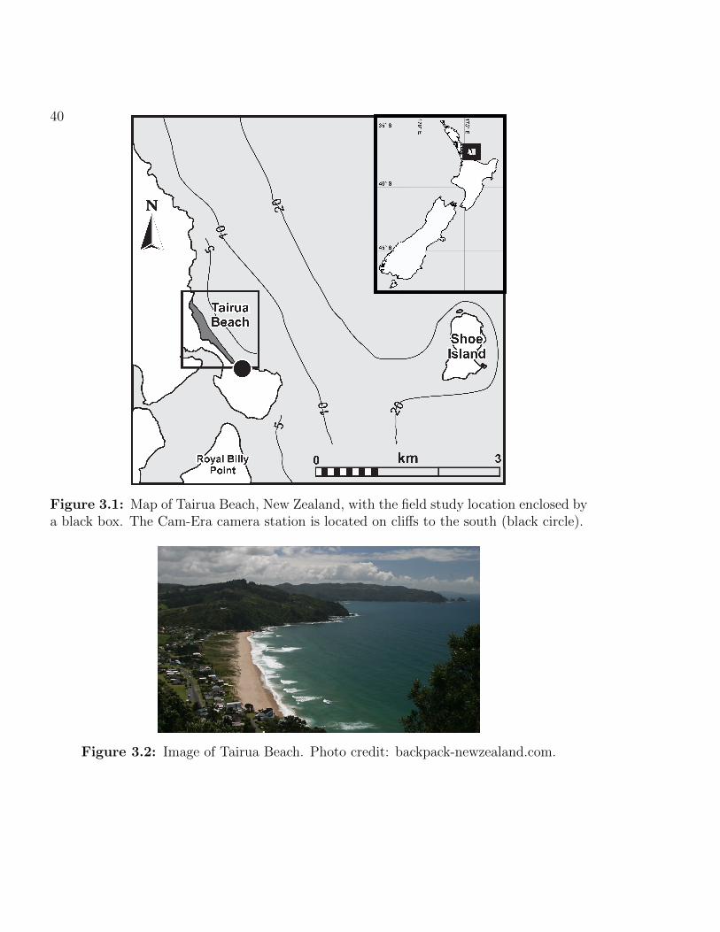
40

Figure 3.1: Map of Tairua Beach, New Zealand, with the field study location enclosed bya black box. The Cam-Era camera station is located on cliffs to the south (black circle).

Figure 3.2: Image of Tairua Beach. Photo credit: backpack-newzealand.com.

subject to medium energy (Hs 1.5 m, Tm 10 s) South Pacific Ocean waves (Almar et al.,

2008). Tairua is an intermediate beach comprised of medium-coarse (D50 ≈ 0.6 mm)

sands. The beach is microtidal, with tide range varying between 1.2 m (neaps) and 2.0 m

(springs) (van de Lageweg et al., 2013).

Tairua is a popular surf and swim beach, with lifeguard patrols operating between the

start of December and the end of February. The patrol is operated by Surf Lifesaving

Australia, and focusses on the use of zoned bathing areas. There is a dedicated swimming

area, demarcated by red and yellow flags; outside of this zone, surfing is permitted and

swimming is discouraged. No rip incident statistics are available for Tairua.

Research at Tairua has made use of a long video imagery record (since 1999). Many

studies at Tairua have therefore used images to quantify other phenomena, including

beach cusp morphodynamics (Almar et al., 2008), shoreline-sandbar coupling (van de

Lageweg et al., 2013), and rip currents (Gallop et al., 2009, 2011). For the purpose of

this thesis, Tairua is used only for development of imaging algorithms in Chapter 5, as

imagery was freely accessible at the onset of the project.

3.2 Perranporth Beach, Devon, U.K.

Perranporth Beach, located in the southwest of England (Figure 3.3), is a 3500 m-long

beach comprised of medium (D50 ≈ 0.3 mm) sand (Austin et al., 2014). The beach has a

wide (500 m) intertidal area at the southern end, which narrows into a 250 m wide

intertidal area in the northern part. At high tide, the beach can become separated into

two distinct beaches by a rocky cliff outcrop half way along. The site is macrotidal, with

a mean spring tidal range typically around 6.3 m (Austin et al., 2014). The beach faces

west-north-west towards the Atlantic and is subject to medium wave energy conditions

with mean significant wave heights (Hs) and peak periods (Tp) of 1.6 m and 10.5 s,

respectively (Austin et al., 2013). The beach often exhibits multiple rip currents,

typically spaced O(200 m) alongshore (Figure 3.4).

41

Perranporth is a popular swimming and surf beach, and holiday destination. The beach

is patrolled by the RNLI during summer, and some public holiday weekends throughout

the year. The beach patrols are conducted by the RNLI, who also provide static signage

at entry points to the beach and flags as a means of segmenting activities in the

surfzone. The signs at likely entry points to the beach outline the patrol information as

well as the likely hazards at that location, such as rip currents or strong tidal currents.

In addition, the signs outline any prohibited activities, such as kite surfing. The RNLI

also use red and yellow flags to indicate bathing areas, and set up their patrol lookout

station between these flags. In addition, black and white flags are used to indicate craft

zones, red flags are used to indicate dangerous conditions whereby people should not

enter the water, and orange flags are used to indicate the prohibition of inflatables. In

addition, mobile hazard-specific warning signs are used on the beach in locations where

strong rip currents have been identified. Over a five year period between 2009 and 2013,

there were 250 rip related rescues at Perranporth (approx. 65% of total rescues). Of

these rip rescue events, the RNLI estimate that without their intervention, 16 events

would have resulted in loss of life.

Research on surfzone currents at Perranporth is well established, through a number of

field deployments (Austin et al., 2009, 2010, 2013, 2014; Scott et al., 2014). In particular,

the dynamics of rip currents have been studied intensely at this site, as have the

demographies of those rescued from rip currents (Woodward et al., 2013). To a lesser

extent, research has also focussed on suspended sediment transport and swash processes

(Masselink et al., 2005; Masselink and Russell, 2006; Thorpe et al., 2013). There is also a

nucleus of research focussing on nearshore bathymetric estimation using video imagery

(Bergsma et al., 2014, 2016). In this thesis, Perranporth is used as the primary site for

the development of synoptic typing methods in Chapter 6. Field data was collected here,

and it forms a substantial part of Chapter 7, where flow regimes are compared to wave

breaking patterns. Finally, rip incident data from the RNLI for Perranporth was used to

inform hazard estimation in Chapter 8.

42

3.3 Ngarunui Beach, Raglan, New Zealand

Ngarunui Beach, located on the west coast of New Zealands North Island (Figure 3.5), is

a 2000 m-long, double-barred dissipative beach comprised of medium (D50 ≈ 0.3 mm)

black (iron) sand (Sherwood and Nelson, 1979). The beach fronts a steep,

well-established dune ridge, and is laterally confined by a rocky headland at the southern

tip and a tidal inlet at the northern edge (Huisman et al., 2011). The predominantly

Figure 3.3: Map of Perranporth, U.K., with the field study location enclosed by a blackbox. The black circle shows the position of the Argus camera station, and the star thedirectional Waverider wave buoy.

43

Figure 3.4: Image of Perranporth Beach, with multiple clearly identifiable rip channelsalongshore [dark, shore-normal streaks intersecting the breaking waves]. Photo credit: S.Pitman.

mesotidal beach (tide range ≈ 1.8 m neap, ≈ 2.5 m spring) faces northwest into the

Tasman Sea and is routinely subject to energetic wave conditions (Hs = 1.8 m, Tm = 8

s) (Gorman et al., 2003). The headland at the southern end refracts the dominant wave

field (propagating from the south west) into a slightly more shore–normal approach at

the beach itself.

Ngarunui is a popular beach for swimming, surfing and fishing, and has lifeguard cover

between October and March. The patrol is operated by Surf Lifesaving Australia, and

focusses on the use of zoned bathing areas. There is a dedicated swimming area,

demarcated by red and yellow flags; outside of this zone, surfing is permitted and

swimming is discouraged. There are also static signs at entry points to the beach

outlining the main hazards at that particular site, such as large shorebreaks, rip currents

44

and submerged rocks. Of 258 rescues over a five season period (2010-2015), 212 (82%)

were attributed, at least in part, to rip current activity.

The selection of Ngarunui as a study site offers the novel opportunity to study rip

hazard on a high energy beach. In addition, video monitoring has been in place at

Ngarunui for a comparatively short amount of time (established 2007), meaning

Ngarunui has received less attention by researchers than Perranporth. The introduction

of the monitoring system has underwritten a number of studies into swash oscillations,

shoreline dynamics, groundwater seepage and wave energy transformations at the site

(Huisman et al., 2011; Guedes et al., 2013). There has been much recent interest in

infragravity swash and resultant current pulsations at infragravity frequencies at the site

(Guedes et al., 2013). Unlike Perranporth, no studies have attempted to quantify which

hydrodynamic conditions are conducive to hazardous rip formation, nor the

demographies of rip victims at Ngarunui. In this thesis, field data was collected for

Ngarunui, and it forms a substantial part of Chapter 7, where flow regimes are compared

to wave breaking patterns. Furthermore, rip incident data from SLSNZ for Ngarunui was

used to inform hazard estimation in Chapter 8.

45

46

Figure 3.5: Map of Ngarunui Beach, New Zealand, with the field study location enclosedby a black box. The black circle shows the position of the Cam-era video monitoringstation.

Figure 3.6: Image of Ngarunui Beach. Photo credit: aa.co.nz.

Chapter 4

Data & methods

This chapter details how Lagrangian, hydrodynamic, remote sensing and rip incident

data were compiled and processed for the thesis. The methods discussed herein are

standard processing techniques that were used, whereas new methodologies pioneered

during this thesis are discussed separately in the relevant results chapters that follow.

4.1 Data

Two field campaigns were carried out in the course of this research at Perranporth from

16—19 May 2014, coinciding with spring tide; and Ngarunui between 10—11 Feb 2015,

midway between spring and neap tides.

4.1.1 Lagrangian rip current data

Rip currents can be highly mobile, with channels often shifting laterally over O(5 m) in

relatively short (tidal) timescales (Quartel, 2009), but equally, they can persist over long

(seasonal) timescales (Holman et al., 2006). As a result of the channel mobility, when

using Eulerian measurement (the deployment of fixed rigs), it is difficult to ensure that

47

the rig is positioned centrally in the rip channel. There is also a high chance that the rip

channel may move during the course of measurement. Furthermore, a fixed rig by nature

can only measure at one point. All these factors combine to hinder accurate

measurement of rip channel flow velocities. For these reasons, there is a growing body of

literature on rip currents whereby the primary means of data collection is Lagrangian

(MacMahan et al., 2010; Austin et al., 2010, 2014; McCarroll et al., 2014). Indeed,

Castelle et al. (2016b) note that this shift to Lagrangian measures is reminiscent of early

rip studies (e.g., Shepard et al., 1941; Shepard and Inman, 1950), where observations

were made of floating objects.

The Lagrangian approach that currently dominates the literature is the use of

GPS-tracked surfzone drifters. Schmidt et al. (2003) designed a drifter from watertight

PVC tubing, that promoted a low (submerged) centre of gravity, and therefore was

quickly self-righting in the surfzone. The drifter had internal GPS components, and an

external GPS antenna. It also incorporated a PVC plate on the bottom, to dampen

vertical motions. The design was modified by MacMahan et al. (2009) with the addition

of three vertical stabilising fins, and the externalisation of the GPS equipment. This

revised design used small off-the-shelf handheld GPS devices, contained within a

waterproof box, mounted on the mast. The addition of external fins improved the

drifters ability to track the currents (MacMahan et al., 2009). A number of studies have

since used variations of the modified design (MacMahan et al., 2010; Austin et al., 2013;

Scott et al., 2014; Gallop et al., 2015, 2016a; McCarroll et al., 2014).

Perranporth

The drifters used at Perranporth were a combination of both designs, including vertical

fins but internalised GPS components (Figure 4.1). The main body was made from 120

mm diameter PVC pipe cut to lengths of 400 mm, with three PVC vertical fins (85 mm

× 300 mm) attached to the outside. A 400 mm vertical damping plate was affixed to the

bottom. The top of the main PVC pipe had a removable bung lid, upon which the mast

was affixed. The lid was sealed with o-rings and three screws into the main body. The

48

49

Figure 4.1: Photograph of the GPS drifters during fieldwork at Perranporth. Withoutballast, the drifters stand 1200 mm in height. The design is modified from Schmidt et al.(2003) and MacMahan et al. (2009). Photo credit: S. Pitman.

mast was a hollow tube 45 mm in diameter and 750 mm in length, atop of which sits a

140 mm aluminium disc and the GPS antenna. The disc reduces the amount of GPS

backscatter from the ocean that is able to reach the GPS antenna itself. From the

antenna, a cable runs through the interior of the mast to the GPS components in the

main body. A ballast weight was fixed to the bottom of the blanking plate, and a

buoyant float affixed to the main body, to achieve the correct buoyancy and floating

depth. When deployed in seawater, the waterline on the drifter was level with the lid of

the main compartment.

The OEMStar low cost single frequency GNSS receiver was used to collect raw L1 GPS

carrier phase signals, which were logged at 1 Hz on an Antilog serial data logger. The

raw signal was post processed using the RTKLIB programme, against data from a static

Trimble base station located on Droskyn Point (Figure 3.3), reducing the positional error

from 1.5 m to < 0.3 m. MacMahan et al. (2009) demonstrated the method to be

appropriate in resolution of flows on O(0.05 ms−1).

At Perranporth, five drifters were used resulting in a total of 195 deployments over the

four days, during 4-hour periods centred on low tide (Figure 4.3). The initial deployment

each day consisted of simultaneous deployment with approximately 30 m spacing

between individual drifters, in order to identify the main location of the offshore current.

From that point forward, drifters were predominantly deployed individually by field

assistants into the rip channel and feeder areas, in water depths of up to 1 m; with entry

times recorded by an observer on the beach. Drifters were also deployed on sand bars

either side of the main channel in order to maximise coverage of the entire circulatory

system. Occasionally, water depth hindered these deployments, and subsequently some

drifters were deployed by an Inflatable Rescue Boat (IRB) seaward of the bars. Drifters

were retrieved (by assistants or IRB) when they entered water too shallow to allow

free-floating, or when they washed along- or offshore to such an extent that it exited the

study area or entered the area preferentially marked by the lifeguards for bathing.

Retrieved drifters were immediately redeployed.

50

Ngarunui

The drifters used at Ngarunui were provided by the University of Waikato, and mirrored

the MacMahan et al. (2009) design (Figure 4.2). The GPS unit sat in a waterproof box,

affixed to a platform on top of the mast. Rather than a GPS chip and separate aerial,

these drifters used handheld, off-the-shelf GPS units, with internal powerpack, receiver

and logging capabilities. The GPS unit used here was the QStarz BT-Q100eX, which

was used to measure latitude and longitude (as opposed to raw L1 carrier phase signals)

at 1 Hz. MacMahan et al. (2009) showed that such handhelds exhibit positional errors of

O(2 m) when stationary, and a test on a stationary drifter confirmed this with mean

horizontal error and standard deviation of 3.78± 1.20 m. The stated manufacturer

velocity accuracy for the units is 0.1 ms−1.

Ten drifters were used at Ngarunui, and a total of 38 deployments were made over two

days, during 3-hour periods centred around both falling and rising mid-tides

(Figure 4.5). Here, drifters were also initially deployed simultaneously in one alongshore

array. Thereafter, they were again primarily deployed individually after retrieval by field

assistants into the rip channel and feeder areas, in water depths up to 1 m. Drifters were

retrieved (by assistants on foot or jet-ski) when they entered water too shallow to allow

free-floating, or when they washed along- or offshore to such an extent that it exited the

study area or entered the area preferentially marked by the lifeguards for surfing.

Retrieved drifters were immediately redeployed.

Drift classification

Each individual deployment was classified visually into one of four categories: 1) linear

exit; 2) circulation then exit; 3) circulation with no exit; or 4) other. These classifications

are similar to those used in other studies (MacMahan et al., 2010; Austin et al., 2013;

Scott et al., 2014; Gallop et al., 2015, 2016a; McCarroll et al., 2014). A linear exit was

defined as the drifter moving offshore immediately from the time of deployment, to

beyond the edge of the surfzone. Circulation then exit was when drifters had a

51

Figure 4.2: Photograph of the GPS drifters during fieldwork at Ngarunui. Photo credit:S. Gallop.

significant portion of onshore movement before moving offshore, or when the drifter

made at least one complete re-circulation before moving offshore beyond the edge of the

surfzone. Circulation with no exit was defined as movement contained within the

surfzone. Under this condition drifters would typically rotate 3 or 4 times over periods

52

O(15 mins) before washing alongshore or onshore. In an extreme case at Perranporth,

one drifter recirculated 13 times over 80 mins before washing alongshore. Other was

defined as occasions when the drifter washed ashore, or travelled significantly alongshore

within the surfzone, without circulation in or around the rip channel.

4.1.2 Hydrodynamics and bathymetry

Perranporth

Sea-level data from the Port Isaac tide gauge (36 km north east of Perranporth) were

obtained from the Channel Coastal Observatory (CCO) online repository

(www.channelcoast.org). Wind and wave data were also obtained from the CCO, with

waves measured using a directional wave rider buoy approximately 1 km offshore of

Perranporth in 14 m water depth. All data was collected at 30 minute intervals.

The hydrodynamic conditions during the study were typical of Perranporth and during

the deployments, Hs reached 1.5 m on the final day, with lower energy conditions (0.5 m

< Hs < 1.25 m) during the other days. Breaking wave heights were unavailable, but

qualitatively estimated to be in the region of 0.5-1 m during the study. Maximum Tp

coincided with the highest waves on the final day, with fluctuations between 8 and 12.5 s

over the 4-day data collection period (Figure 4.3c). The spring tide range was 6.4 m.

The incident wave field propagated approximately shore-normal throughout

(Figure 4.3d). Wind was onshore over the first three days, with a low wind speed (U =

2.5 m s−1) on the first two days and high larger wind speeds (U = 8.8 m s−1) on third

day. On the final day of the experiment, a weak (U ≈ 1 m s−1) offshore wind prevailed

(Figure 4.3e—f). The beach exhibited a typically double bar state (Masselink et al.,

2014) with the inshore and outer bars at c. 500 and 800 m offshore of the mean high

water springs shoreline, respectively.

The bathymetry was measured on 17 May 2014 using an IRB, fitted with a single-beam

echosounder. Bathymetry was collected in cross-shore profiles spaced 25 m apart over

the nearshore bar, and 50 m offshore of the outer bar. Subaerial beach topography was

53

54

Figure 4.3: Summary of field conditions from 16 to 20 May 2014 at Perranporth Beach,with vertical grey bars indicating drifter deployments: a) water level Htide; b) significantwave height Hs; c) peak wave period Tp; d) incident wave direction θ; e) wind speed U ;and f) wind direction WDir. Red lines indicate the shore-normal direction. ODN refers toOrdnance Datum Newlyn, which is approximate Mean Sea Level in the UK.

Figure 4.4: Bathymetry and drifter data for the field experiment with white boxesindicative of study area and solid black line is 0 m ODN. (a) The merged bathymetricand topographic data, measured on 17 May 2014. (b) The residual morphology. (c) Theoverlay of merged, rectified images from the Argus camera onto the bathymetry.

measured using an All-Terrain Vehicle (ATV) fitted with RTK-GPS, in alongshore lines

spaced 10 m apart (Figure 4.4).

Ngarunui

Sea-level data from the Kawhia Wharf tide gauge (32 km south of Ngarunui) was

obtained from Waikato Regional Council. The Kawhia record is more complete than the

Raglan record, and tidal heights are comparable (typically within 0.2 m). Offshore wind

and wave conditions were obtained from the nzwave 12 wave forecast using

WAVEWATCHv3.14, run by NIWA. At the grid point closest to Ngarunui, hourly data

are available from longitude –37.777834 and latitude 174.66760, at 53 m water depth.

The Ngarunui study also encapsulated average wave/tide conditions. Hs ranged between

1.4 m and 1.9 m during deployments (Figure 4.5b), slightly below the annual average

(Hs = 2.2 m). Breaking wave heights were unavailable, but qualitatively estimated to be

in the region of 1-1.5 m during the study. Tp during deployments ranged from 12 to 15

secs, with the shortest period waves occurring on 11th Feb, and the longest period on the

55

10th Feb (Figure 4.5c). Wave propagation estimated by the hindcast was predominantly

from the south–west (Figure 4.5d), however, the headland at the southern end of the

beach (Figure 3.5) acts to refract waves around to a slightly more shore–normal

approach at the beach itself. Wind speed (Figure 4.5e) fluctuated between 7 and 9 m s−1

during deployments, with direction offshore for both days (Figure 4.5f).

The intertidal beach bathymetry was surveyed on 5 Feb using RTK-GPS, in alongshore

transects. This intertidal bathymetry covers the cross-shore extent between -700 m and

-450 m (Figure 4.6), which approximately covers the area above the MLW mark. Further

offshore, the subtidal bathymetry used for Ngarunui can be considered as a general

overview, rather than specific to the study. Data were collected via various methods on

dates between 2008—2013, and combined with Chart data from 1977 by Harrison and

Hunt (2014), and it will therefore have changed by the time of the study. As a result,

bathymetry cannot be used as indicative of channel location, and is presented purely to

give an overview of general slope. The composite subtidal bathymetry comprises

elements of boat-mounted multibeam echosounder surveys, LiDAR surveys,

jetski-mounted single beam echosounder surveys, in addition to the digitisation of

navigational charts and orthophotos. Measurements were exported to a 1 m grid. The

two datasets have been merged and used to present subtidal bathymetry in this thesis

(Figure 4.6).

4.1.3 Video imagery

Tairua

Tairua has been monitored since 1999 by the NIWA Cam–Era scheme, located on Paku

Hill at the southern end of the beach (Figure 3.1). The camera is located at 70 m above

chart datum (van de Lageweg et al., 2013), affording good coverage of the dune,

beachface and nearshore zone for the entirety of the beach, excepting the first 50 m

which is hidden by outcrops of Paku Hill (Almar et al., 2008).

56

57

Figure 4.5: Summary of field conditions from 8 to 13 Feb 2015 at Ngarunui Beach, withvertical grey bars indicating drifter deployments: a) water level Htide; b) significant waveheight Hs; c) peak wave period Tp; d) incident wave direction θ; e) wind speed U ; andf) wind direction WDir. Red lines indicate the shore-normal direction. Tidal heights arereference to MSL.

Figure 4.6: Bathymetry data for Ngarunui. The solid black line represents MSL. (a)The general bathymetric data merged with topographic data measured on 8 Feb 2015. (b)The residual morphology. (c) The overlay of merged, rectified images from the Cam-Erastation onto the residual morphology.

Perranporth

Perranporth is monitored by a set of three Argus cameras located on Droskyn Point at

the southern extreme of the beach (Figure 3.3), 48 m above mean sea level (Huntley

et al., 2009). The first two cameras were installed in 1996, with the third installed in

2010 (Scott et al., 2014). This study uses half-hourly, geo-rectified 10-minute time

exposure (timex) images (Figure 2.3) in the local Argus co-ordinate system.

It is unfortunate that the Argus camera was unserviceable for the period 20—23 Jul and

also 6—22 Aug 2013, when a large number of incidents occurred. However, investigation

of the images captured immediately prior to and following these outages showed the

presence of numerous and prominent open rip channels. Furthermore, the wave

conditions between 23 Jul and 23 Aug 2013 were low energy (mean Hs = 1.02 m), with

no storms and therefore it is likely that the prominent open rip channels persisted

throughout the period.

Ngarunui

Ngarunui is monitored by a set of two NIWA Cam–Era video cameras located at the

southern end of the beach (Figure 3.5) at a height of 95 m above mean sea level (Guedes

58

et al., 2013). One camera provides coverage of the outer bar and offshore, with one

focussed on the inner bar, swash zone and subaerial beach. The merged, rectified image

gives coverage of the entire 2 km beach to the boundary with the tidal inlet.

One of the two cameras was unserviceable for the latter half of 2015, and therefore

images from this period are omitted from further analysis within this thesis.

4.1.4 Rip incident data

Perranporth

Rip incident data were supplied for Perranporth by the RNLI for 2009—2013, during

which time RNLI patrols were active between April and October. The RNLI record an

incident every time they intervene. They record time and location, demographic data,

qualitative observations of meteorological and hydrodynamic conditions and, crucially,

information on the cause of the incident (e.g., inexperience, rip currents, tidal cut off,

etc.).

Ngarunui

Rescue, first aid and search data at Ngarunui was supplied by Surf Life Saving New

Zealand (SLSNZ) for 2010—2015 (SLSNZ, 2016), during which time the beach was

patrolled between October and March. This database is compiled by surf lifeguards after

any incident whereby some intervention physical (as opposed to verbal) response is

required. They record the time and location, demographic data, qualitative data on

strength of wind and surf, and a narrative on the activity a person was involved in, as

well as any compounding factors (e.g., poor swimmer, rip currents, etc.).

59

4.2 Methods

4.2.1 Drifter GPS data

The drifter data collected at 1 Hz was initially filtered by location into a 0.1 Hz signal,

to remove noise inherent in the GPS signal that is not representative of the true drifter

path. Velocity was calculated between the new filtered 0.1 Hz dataset, and the velocity

signal was subject to a zero phase, fifth order Butterworth lowpass filter, as in the case

of previous drifter studies (Johnson and Pattiaratchi, 2004; McCarroll et al., 2014), with

a cut off of 0.05 Hz. The positional data is now linearly interpolated back into

observations at 1 Hz, representing the original sample frequency. At this point, the

bearing of the drifter is calculated and recorded at 1 Hz. Then all values are converted

into the Argus co-ordinate system, resulting in latitudes and longitudes converted into a

co-ordinate system based on metres distance from a nominal Argus origin.

The spatial domain in which the drifters circulated was divided into 10 × 10 m cells

(Figure 4.7a; 4.8a) and all drifter data for subsequent discrete time periods were

calculated within these cells. This cell size is appropriate to quantify the circulation

pattern, given that typical scales of rip circulation are O(100 m), and is comparable to

previous studies (MacMahan et al., 2010; McCarroll et al., 2014). Following the work of

Spydell et al. (2007) and MacMahan et al. (2010), observations in the same grid square

were grouped into one independent observation. If the drifter later re-entered the grid

square, it would be considered a new independent observation if it had travelled a

significant distance (defined as the length of the grid square) before doing so. A

re-entering drifter was independent when t > lg/U (MacMahan et al., 2010), where t is

elapsed time, lg is the grid square size and U is the average drifter speed whilst in transit

outside of the gridsquare. Velocity and direction measurements were then calculated for

bins with at least 5 independent observations (Figure 4.7a; 4.8a), following Spydell et al.

(2007) and MacMahan et al. (2010). Velocity calculations (Figure 4.7b; 4.8b) were based

on the mean of independent observations in each grid square (U ′). Following (McCarroll

et al., 2014), the overbar is herein used as a denotation for a value based on a grid

60

Figure 4.7: Bathymetry and drifter data for the Perranporth field experiment with whiteboxes indicative of study area and solid black line is 0 m ODN. (a) Number of independentobservations recorded at 0.1 Hz over the study period, binned into 10 × 10 m grid squares.Grid squares with < 5 observations appear as grey and are not considered further in thethesis. (b) Mean drifter velocities recorded during the experiment. (c) Overall surfzonevorticity over the experiment, with red values indicative of an anti-clockwise horizontalrotation, and blue values indicative of clockwise rotation.

square mean, and the prime symbol denotes the use of independent observations. The 10

s window was used because the maximum drifter speeds from previous Perranporth

experiments (Austin et al., 2009; Scott et al., 2014) were typically around 1 m s−1,

equating to up to 10 m horizontal displacement over a 0.1 Hz window, coinciding to the

initial filtered frequency of drifter positions. This is comparable to the 10 × 10 m cells

that were used to construct the spatial domain for processing. These processing steps are

summarised along with examples of each stage at Appendix A.

The circulation of rip currents is of paramount importance in this study and therefore a

measure of vorticity (Γ) is presented throughout (Figure 4.7c; 4.8c). Vorticity is defined

as the change in orientation of a parcel of water, without change in area or shape

(Molinari and Kirwan, 1975; MacMahan et al., 2010) and is a parameterisation of the

local rotational motion of a fluid, or velocity shear (McCarroll et al., 2014). Vorticity

61

Figure 4.8: Bathymetry and drifter data for the Ngarunui field experiment with solidblack line is MSL. (a) Number of independent observations recorded at 0.1 Hz over thestudy period, binned into 10 × 10 m grid squares. Grid squares with < 5 observationsappear as grey and are not considered further in the thesis. (b) Mean drifter velocitiesrecorded during the experiment. (c) Overall surfzone vorticity over the experiment, withred values indicative of an anti-clockwise horizontal rotation, and blue values indicativeof clockwise rotation.

was calculated using the weighted central difference method (MacMahan et al., 2010), as

follows;

Γ =dv

dx− du

dy(4.1)

where u and v are the vector components of U ′ at point x,y.

62

4.2.2 Bathymetry

The subaerial topography and submerged bathymetry were merged with significant

overlap for quality control (Figure 4.4a). The bathymetry presented here is the residual

morphology (Figure 4.4b), following the approach of Austin et al. (2010). The residual

bathymetry is obtained by subtracting the cross-shore linear trend surface over the entire

intertidal area from the measured bathymetry at that same cross-shore transect. Waves

breaking over a linear surface would be expected to break in a uniform manner, and

therefore the deviations from this linear surface obtained by subtracting from the real

profile act to highlight areas where increased (positive values) and decreased (negative

values) wave breaking would be expected. No post-processing was conducted on

Ngarunui bathymetry, as it was supplied in complete form.

4.2.3 Video imagery

The use of video imagery for quantitative analysis requires an understanding and

application of the various technical transformations to yield results in terms of real world

(x, y and z) location. All imagery for this study was converted from oblique imagery, to

rectified, merged, plan view images. This process was discussed in Section 2.1.1, and a

full technical overview of the process was provided by Holland et al. (1997).

In general, there is potential that the imagery at this frequency aliases the wave group

frequency, which has before been postulated as an important process in controlling rip

current velocity pulses (Shepard et al., 1941; Sonu, 1972; Aagaard et al., 1997). However,

Scott et al. (2014) estimate wave group frequency at Perranporth to be between 25—250

secs, and the chosen image sampling frequency of 600 secs ensures that at least one wave

group is captured per timex image. Furthermore, the nature of the timex image ensures

that the maximum extent of wave breaking is captured, and therefore aliasing effects do

not present a significant problem for later analysis.

63

64

Chapter 5

Synthetic imagery for rip channel

detection

This chapter discusses progress in the development of an automated approach to rip

detection from video imagery and the creation of synthetic images to facilitate this. It is

adapted from the following publication:

Pitman, S.J.; Gallop, S.L.; Haigh, I.D.; Mahmoodi, S.; Masselink, G., and

Ranasinghe, R., 2016. Synthetic imagery for the automated detection of rip currents.

In: Vila-Concejo, A.; Bruce, E.; Kennedy, D.M., and McCarroll, R.J. (eds.),

Proceedings of the 14th International Coastal Symposium (Sydney, Australia).

Journal of Coastal Research, Special Issue, No. 75, pp. 912-916. Coconut Creek

(Florida), ISSN 0749-0208.

5.1 Introduction

The development of coastal imaging systems over the past 30 years has provided huge

opportunity for investigation of the coastal zone through remote sensing. Such systems

65

are an attractive prospect as they are comparatively cheap and are constantly recording

data, under all manner of meteorological and oceanographic conditions. Their use as a

means to detect rip currents was first proposed by Ranasinghe et al. (1999), who noted

alongshore pixel intensity minima locations were coincident with rip channels. Since

then, there have been numerous attempts to automate the detection of rip currents.

Automation is a goal for researchers because video imaging systems, constantly recording

data generate datasets that are too large to manually sift. That said, to date, the

complexity of surfzone imagery has prevented the development of automated detection

methods. Here, the background to video imaging the coastal zone, attempts to automate

rip current detection, and the steps that can be taken to simplify surfzone imagery in an

attempt to make automation possible are all considered.

An overview of past literature dealing with automated rip detection was presented in

Section 2.1, and a brief summary follows here. After the discovery of Lippmann and

Holman (1989) that video imagery provided a useful means of quantifying nearshore

processes using light intensity in time exposure images, numerous studies have linked the

intensity minima to rip detection. A simple alongshore-orientated intensity profile was

first found to work well for simple rip detection scenarios, but failed to cope for more

complex or energetic scenarios (Ranasinghe et al., 1999). The method also suffered a

degree of subjectivity in the selection of analytical thresholds (Holman et al., 2006).

These complications in automated detection meant that many rip detection studies have

instead favoured subjective manual means of rip detection in imagery (e.g. Bogle et al.,

2000; Whyte et al., 2005; Holman et al., 2006; Turner et al., 2007; Quartel, 2009; Orzech

et al., 2010; Murray et al., 2013). The most recent attempt to develop an automated

means of detection was that of Gallop et al. (2009, 2011), but this too ultimately needed

manual cleaning as a result of the complex trends evident in the imagery. With image

complexity being a recurring theme, it is of interest to investigate how pre-processing of

an image may affect its subsequent utility for rip detection. The dominant image type

used for analysis, the timex, is already considered to be filtered as it represents the

time-mean pixel intensity over (typically) a ten minute period, however, there are still

66

large amounts of noise in the imagery (e.g. fouling by dirt or rain on the lens during

acquisition).

Therefore, the overall objective of this chapter is to develop pre-processing image

techniques to improve the reliability of automated rip channel detection in video

imagery. Here, two case study sites are used; the macrotidal, intermediate, low tide

bar/rip beach at Perranporth and the microtidal, intermediate embayed beach at Tairua.

In order to address the objective, there are a number of sub-objectives: (1) To assess the

utility of image filtering as a method of removing noise and image fouling in video

imagery; (2) To develop a (semi)automated approach to rip detection, and (3) To explore

the use of synthetic imagery as an aid to automated rip detection. The contents of this

chapter are heavily weighted towards methodology, as unless stated, the methodology

was developed as part of this work, and is not simply the employment of established

methodologies. This chapter focuses on imagery from Tairua and Perranporth.

5.2 Methodology

This section will first outline the novel method for pre-filtering surfzone imagery, before

outlining the methods employed to create a synthetic image of the surfzone for

subsequent processing. Subsequently, a new means of automating detection on the

synthetic imagery is explored.

5.2.1 Image rectification

The first stage in rip detection is generally to rectify the images, using standard

photogrammetric transformations between ground and image co-ordinates (Holland

et al., 1997), as discussed in Section 2.1.2 and this is the approach applied here. The

image is subsequently cropped to minimise peripheral noise and re-orientated so that the

shoreline runs parallel to the x-axis (Figure 5.2a). It is important that the image

67

includes not only the breaking zone, but also a portion of the offshore environment, so

that the breaking region can be delineated later (Section 5.2.4).

Pixel resolution of the original imagery has an important bearing on the ability to make

quantitative measurements from the resultant rectified image. A typical coastal imaging

camera will image in an array of 1024 × 768 pixels, with spatial resolution a function of

the projection from a pinhole lens, through the pixel and onto the ground footprint of

that pixel (Holman and Stanley, 2007). The result of this transformation is that

near-camera features are imaged with high spatial resolution (pixel = ≈ 0.05 m), but

resolution decreases linearly with range such that alongshore resolution 1,500 m from the

camera is of the order 30 m (Aarninkhof et al., 2003). Cross shore resolution is much

better conserved at range, likely to be < 5 m at a distance of 1,500 m (Aarninkhof et al.,

2003). Generally, long-shore features have much smaller spatial gradients than those in

the cross-shore, requiring less resolution to resolve. In this study, all features are

typically within 500 m of the camera, and the resolutions quoted are more than sufficient

to resolve rip currents with length and width scales typically around 100 m and 30 m,

respectively.

5.2.2 Image filtering

Simple single-image filtering of nearshore images has not been widely used before,

because the prevalent image type used for analysis is the so called timex image, which

represents the time-mean of intensity in all frames collected at 2 Hz over a 10-minute

period (Holman and Stanley, 2007). This constitutes a form of average filtering during

the image acquisition stage; however, the resultant image may still include background

noise or erroneous data. One such example is raindrops on the lens covering, which

would appear in the rectified image, giving a false intensity signature for the pixel(s)

concerned. Studies using video images tend to reject imagery where raindrops are visible

on the lens for this reason. Holman et al. (2013) described how consecutive images in a

time series can be used to create a running-average estimate (cBathy). cBathy uses wave

celerity to estimate bathymetry, and the use of this running-average filter was successful

68

in removing fouling from subsequent images, such as rain drops or sun glare. Despite the

assumption that a timex image is already prefiltered, it still contains noisy signals,

representative of a very dynamic surfzone. Furthermore, inclement weather still appears

as fouling in the imagery. Therefore, there is a need to pre-filter the image before

processing, rather than relying on filtering the signal that is extracted as a result of

processing.

The first stage to create a synthetic image is filtering the parent image. A common

approach to filtering is the use of high- and low-pass filters. These operate in the

frequency domain of the image, akin to Fourier transforms. High frequency noise is

introduced to imagery by sharp intensity transitions, such as edges observed at the

shoreline. These high frequency signals can be smoothed using a lowpass filter (Tomasi

and Manduchi, 1998), attenuating the high frequency components and therefore blurring

the image (Gonzalez and Woods, 2008).

In simple cases, where only a few raindrops have fouled the image, spatial filtering can

remove the effect of this noise. When the fouled image is rectified, the previously small

element of noise (the rain drop), is projected across a wide area (e.g. Figure 5.1a), as a

result of the transformation between image co-ordinates [u, v] and real-world

co-ordinates [x, y, z]. A Gaussian lowpass filter (Tomasi and Manduchi, 1998) is applied

(mask = 15 × 15, σ = 10) to the rectified image (Figure 5.1b). Subsequently, pixel

intensities from the same transect of pixels in each image are extracted (Figure 5.1c).

The maximum gradient in intensity profile is used as an estimation of the onset of wave

breaking. In the unfiltered image, large errors are evident in the detected location of

wave breaking (Figure 5.1d) wherever rain fouls the lens. In contrast, the errors are

much reduced in the profile extracted from filtered imagery.

This example highlights the benefits to be gained from image manipulation prior to

processing, such as the removal of small patches of lens fouling. As these sharp intensity

transitions are often expected to represent the very feature we wish to investigate, such

as the edge of a rip channel, filtering can smooth these features yielding more accurate

results.

69

70

Figure 5.1: (a) Rectified timex image of Tairua Beach, New Zealand. Rain drop foulingis evident in the region of the blue transect line. (b) Filtered version of (a) with redtransect line. (c) Intensity profiles for both transect lines, with the maxima marked byhorizontal lines. (d) Onset of wave breaking detected alongshore using intensity maximatransects, as per (c).

5.2.3 Shoreline detection

Before proceeding any further, it is important to isolate the surfzone in the imagery. The

surfzone is bounded by the shoreline on one side, and the maximum intensity of wave

breaking (henceforth referred to as the barline) on the other. The shoreline and barline

are used here to mask the outer areas of the image, as rips will not occur outside of the

breakers or on the beach. Colour is a useful way to segregate objects and is used here as

a means of detecting the shoreline. However, the absolute colour recorded in an image is

susceptible to a number of conditions (e.g. illumination, shading, and reflectivity) that

may result in depicted colour being different to actual colour (Gevers and Stokman,

2003). In contrast, normalised colour (the difference between percentage of red, green

and blue hues in each pixel) was almost invariant to changes in lighting and camera

positions (Gevers and Smeulders, 1999). Therefore, rather than using absolute colour,

this approach uses colour histograms derived from all available pixels in the imagery.

The image is segmented into 3 broad clusters using k-means clustering (Wang and

Adelson, 1994). This method assigns each pixel a location in space, and then partitions

the image into 3 clusters, based on the signature of the RGB value of pixels

(Figure 5.2b). The cluster with a dominance of red pixels is invariably associated with

the darker colours of the beach, and contrasts against the blues and greens associated

with swash and breaking waves. The boundary between the red cluster and its nearest

neighbour is therefore used as an estimate of shoreline position for the remainder of the

algorithm steps (Figure 5.2c).

5.2.4 Barline position

When attempting to detect the barline (i.e. the offshore extent of wave breaking), colour

images are less useful. In graycale imagery the sand bars show as white pixels in images

as waves break over the shallower sea bed (Lippmann and Holman, 1989), making an

obvious contrast against a darker, offshore area. If colour imagery is used, assessment of

71

72

Figure 5.2: (a) Original rectified timex image from Tairua Beach, New Zealand (NIWA).The image is orientated so that shoreline runs along the x-axis. (b) The image is firstsegregated into three groups, corresponding to the dominant red, green, and blue pixelclusters. The boundary between beach and breaking zone is depicted well by this method,and is therefore used (c) as an approximation of shoreline. (d) The image is then convertedto grayscale for further processing.

the absolute colour is required, detracting from the algorithms ability to work at

multiple sites without calibration.

Although it is possible to detect a change from the aquamarine colours of the offshore

area to the lighter areas of wave breaking, this study has found it to more accurate to

make use of grayscale imagery for the reasons stated (Figure 5.2d). The image is

therefore converted to grayscale, and the dynamic range (the contrast between dark and

light intensities) is stretched. The intensity profile of each column of pixels is then

measured (Figure 5.3a), with the onset of wave breaking identified as the first peak

above a significant threshold in the intensity profile. That is to say, the algorithm looks

for the first sharp change between darker offshore areas and lighter pixel intensities. This

threshold needs a sensitivity analysis within and between sites, but is currently set at

0.2, on a normalised intensity scale between 0 and 1. This intensity threshold is to

ensure that the detected signal is above any offshore generated noise in the intensity

profile, and represents a significant feature (the onset of depth-induced wave breaking).

This is henceforth simply referred to as the barline. The location of this significant peak

is calculated for every column of pixels in the image, and the resulting indexed locations

are lowpass filtered to give a coherent barline (Figure 5.3b). This increase in pixel

intensities has previously been deemed an appropriate indication of bar position (Bogle

et al., 2000), however, the threshold chosen will vary according to site.

The accuracy of the methods outlined above for bar- and shoreline detection were tested

against expert-user digitised datasets of positions. The employment of an expert-user

allows for ‘ground truth’ positions to be ascertained, using a trained person to digitise

the features of interest directly. In this case, the author acted as the expert-user. Both

methods outlined above show good correlation with manual detections (Figure 5.4).

Comparison between manual and automated shoreline detections were correlated at

r2 = 0.87, with a slightly lower correlation (r2 = 0.81) in barline detection. Both

methods were deemed to be of a suitable level of accuracy for surfzone delineation as a

stage on the automated detection algorithm.

73

74

Figure 5.3: (a) Derivation of barline for one individual column of pixels. The pixels areshown in the bar below the figure, with the respective normalised pixel intensity alongthat bar shown above by the blue line. The 0.2 threshold is marked (dashed line) and thefirst peak in intensity above that threshold (red line) is stored as the barline location. (b)Repetition of this method for every column of pixels in the image gives an estimate of thelongshore variable barline.

Figure 5.4: Scatter intensity plot of algorithm and (a) manually derived shoreline and(b) barline locations, with white line representing 1:1 correlation. The colour is indicativeof the number of observations at that location.

5.2.5 Creation of a synthetic image

Having isolated the surfzone, the creation of a synthetic image requires the segmentation

of the surfzone into two categories that identify areas of wave breaking and non-breaking

(rip channels). This ultimately creates 4 distinct zones in the image as a whole: beach,

rip channels, breaking waves, and offshore. The offshore boundary of the surfzone is the

limit of wave breaking which is defined by the first significant increase in the pixel

intensity gradient (Bogle et al., 2000). The landward boundary of the surfzone is

determine by the shoreline. This is detected using segmentation based on 3-banded

k-means clustering (Wang and Adelson, 1994). This method identifies the beach by the

dominance of the red pigmentation in the RGB signature. The surfzone must then be

separated into rip channels and wave breaking regions. This is done by thresholding the

extreme intensity values of the remaining zone (between the detected bar- and

shoreline), and using the mid-point as a cut-off to separate into two distinct zones.

The image is now composed of 4 distinct zones (Figure 5.5b). Subsequently, it is

important to return the now zoned image into something that visually represents a

normal image, so that existing surfzone imaging algorithms can be applied to it. These

75

algorithms would fail on the segmented image, as a result of the lack of colour and the

sharp transitions between zones. In order to return the image to a visually correct state,

the outline of the zones are overlaid onto the original image, and the RGB values for each

pixel within the various zones are recorded. This allows the creation of a pixel colour

historgram that is epresentative of the colours observed in each zone (Figure 5.5c—f).

For each zone in turn, it is then possible to reconstruct the dominant colour using the

normal distribution of red, green and blue pixels in the histogram. In order to avoid

uniform colours for each zone, the algorithm randomly selects a red, green and blue value

from the normal distribution, weighted towards the higher probability occurrences on the

normal distribution. It is then able to replace all pixels in the zoned map with an

appropriate colour, representative of the real image (Figure 5.5g). The final result is that

all original pixels are replaced with visually similar, but less noisy synthetic pixel zones.

5.2.6 Minima detection

Minima detection focusses on the area between the shoreline and barline. The pixel

intensities in the grayscale version of the original image are first lowpass filtered to

remove localised noise (Figure 5.6a).

Energetic wave breaking on the edge of channels creates very high intensity areas. As a

result of this, sometimes the area along the bar can appear as a localised intensity

minima between these high intensity areas, despite the fact that it is light in colour and

does not correspond with a channel. Therefore, the lightest 50 % of pixels are removed

(Figure 5.6b). This has the effect of removing areas of wave breaking, and thus the

localised minima over bars.

The algorithm then detects minima in 4 directions across the image: gradient is assessed

across each of the 8 neighbouring pixels (Figure 5.6c). If the algorithm detects a local

minimum in any direction, then the observation is stored, as long as it falls within the

thresholded image (Figure 5.6d).

76

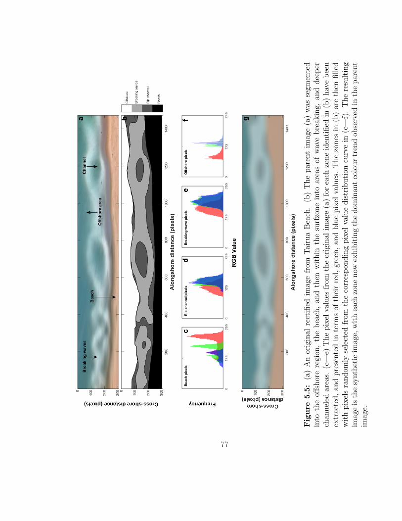
Fig

ure

5.5

:(a

)A

nor

igin

alre

ctifi

edim

age

from

Tai

rua

Bea

ch.

(b)

The

par

ent

imag

e(a

)w

asse

gmen

ted

into

the

offsh

ore

regi

on,

the

bea

ch,

and

then

wit

hin

the

surf

zone

into

area

sof

wav

ebre

akin

g,an

ddee

per

chan

nel

edar

eas.

(c—

e)T

he

pix

elva

lues

from

the

orig

inal

imag

e(a

)fo

rea

chzo

ne

iden

tified

in(b

)hav

eb

een

extr

acte

d,

and

pre

sente

din

term

sof

thei

rre

d,

gree

n,

and

blu

epix

elva

lues

.T

he

zones

in(b

)ar

eth

enfilled

wit

hpix

els

random

lyse

lect

edfr

omth

eco

rres

pon

din

gpix

elva

lue

dis

trib

uti

oncu

rve

in(c

—f)

.T

he

resu

ltin

gim

age

isth

esy

nth

etic

imag

e,w

ith

each

zone

now

exhib

itin

gth

edom

inan

tco

lour

tren

dob

serv

edin

the

par

ent

imag

e.

77

78

Figure 5.6: (a) The detected barline and shoreline are used to create a masked image,depicting only the surfzone. The image has also been lowpass filtered. (b) The remainingimage is thresholded so that areas of wave breaking (black section) can be removed fromthe search area. (c) Minima are then located in the remaining areas. Red lines depictthe shore- and bar-line, with blue lines highlighting the search areas. Detected minimaare shown as white lines. (d) This search returns the minima contained within the darkerparts of the image. (e) Significant features detected in the algorithm are stored as coherentrip currents (red features).

5.2.7 Rip grouping

Once individual minima have been detected, the algorithm groups observations into

coherent features. In order to do this, it segregates the image into a grid, with typical

grid sizes being around 2-3 pixels wide, enabling clusters of minima to be grouped into

defined features. Neighbouring grid squares that contain minima observations are

recorded as the same feature (potentially a rip). The process is repeated until no more

distinct features are found. The algorithm then makes an assessment as to whether any

of the detected features are significant. To do this, it looks at their along- and

cross-shore extent. Features which extend over a cross-shore distance greater than 30 %

of the surfzone width at that point are classed as significant. Likewise, features that

extend alongshore over a distance greater than twice the width of the surfzone would be

saved (Figure 5.6e). The cross-shore threshold was particularly important at

Perranporth to remove small features in the intertidal that appeared as a result of the

shallow beach slope.

5.2.8 Application of method

The method was first applied to imagery from Tairua Beach, described in Section 3.1.

The beach is microtidal with a comparatively steep gradient, which made rip features

often appear prominently in the imagery. It also meant the tidal translation over the

image was minimal, meaning the same crop area was applicable over the entire tidal

cycle. The method was secondly applied to imagery from Perranporth Beach, described

fully in Section 3.2. Perranporth is a macrotidal environment, with large tidal

translation rates over a large intertidal area. As a result, analysis was confined to images

centred around low tide, in the field of view of the camera.

In both cases, the algorithm was applied to the original rectified image and the

corresponding synthetic image, created using methods outlined above. The standard

against which these detections were applied is an expert digitisation, which were user

79

digitised images of the rip current, outlining the features the digitiser deemed to be rip

channels, and of interest.

5.3 Results

5.3.1 Automation of rip detection

On occasion at Tairua, the rip currents were too subtle for the algorithm to detect them

(e.g. Figure 5.7a). In the majority of cases, the algorithm was able to detect the minima

related to the rip currents, but there was a bias for over-detection (i.e. far more detected

than was desirable), compared to the expert digitisations. For example, Figure 5.7b

shows four small distinct features considered of interest by expert digitisations, but in

the automated detections on the original image, the algorithm has detected one large

alongshore feature on the left, and one smaller feature on the right. This is a result of

over-detection of minima in the image, and was a trend echoed throughout the dataset.

Qualitatively, the problem is reduced when using synthetic imagery, where detections are

reduced and mirror more accurately the expert digitisations. Despite the improvement as

a result of synthetic imagery, the majority of detections still required a degree of manual

post-processing in order to remove unwanted detections. This was a trend echoed

throughout the majority (>70 %) of the dataset, with the automation alone not being

sufficient. In the majority of cases, the time required to correct inaccuracies far exceeded

the amount of time required to digitise the imagery from scratch.

At Perranporth, the effect of a sweeping tidal zone and shallower beach slope was to

obscure the rip channels somewhat. In order to achieve similar results as for Tairua

detections, the threshold by which the surfzone is turned to a black and white image

(Section 5.2.6) required calibration to a new site. The propensity to over-detect was

magnified at Perranporth (Figure 5.8), increasing the amount of manual cleaning

required. In the majority of cases, individual rip currents were classified by the algorithm

as interconnected along almost the entirety of the alongshore zone in the image. There is

80

Fig

ure

5.7

:T

est

auto

mat

eddet

ecti

ons

from

Tai

rua

Bea

ch.

The

left

colu

mn

show

sex

per

tdig

itis

atio

ns,

and

pro

vid

eth

est

andar

dag

ainst

whic

hth

eau

tom

ated

det

ecti

ons

shou

ldb

eju

dge

d.

The

mid

dle

colu

mn

show

sdet

ecti

ons

mad

eon

the

orig

inal

imag

ery.

The

righ

tco

lum

nsh

ows

det

ecti

ons

mad

eon

the

synth

etic

imag

ery.

Eac

hro

w(a

—d)

show

sim

ages

from

adiff

eren

tti

me.

81

Fig

ure

5.8

:T

estau

tomated

detection

sfrom

Perran

porth

Beach

.T

he

leftcolu

mn

show

sex

pert

digitisation

s,an

dprov

ide

the

standard

against

which

the

autom

ateddetection

ssh

ould

be

judged

.T

he

mid

dle

colum

nsh

ows

detection

sm

ade

onth

eorigin

alim

agery.T

he

right

colum

nsh

ows

detection

sm

ade

onth

esy

nth

eticim

agery.E

achrow

(a—d)

show

sim

agesfrom

adiff

erent

time..

82

an image seam between two cameras present in Perranporth imagery that may have

contributed to this. More important, however, was the shallow nature of the beach that

resulted in an unclear definition between dry sand, wet sand, and surfzone. The

algorithm became highly sensitive to the detected shorelines and barlines when applied

to the Perranporth dataset. The result was an even higher proportion of images in the

Perranporth dataset requiring manual post-processing to be of quantitative value.

The selection of thresholds is the dominant factor behind the inability of the method to

cope with inter- and intra-site conditions. Despite it being the main factor in the

algorithms inability to be deployed at any site, the inclusion of thresholds appears to be

a necessary step in the extraction of quantitative data from imagery (Ranasinghe et al.,

1999; Alexander and Holman, 2004). One major step forwards would be in the inclusion

of some means empirically derive the threshold for a particular site based on a sample

set of images, yet this appears to be some way off, not least because of the number of

different thresholds currently required to extract quantitative data. One such threshold

is the value chosen to isolate darker areas in the surfzone. A sensitivity analysis of this

method is presented as Figure 5.9. This thresholding is required as part of the process to

avoid detections of localised minimas over areas of wave breaking, when the area actually

of interest is localised minima in channels. Figure 5.9 shows an original image and the

threshold used at each stage. In the middle column, the threshold is applied to the

surfzone (delineated by the bar- and shorelines), to convert the image into black and

white areas. Black areas are constructed from areas lighter than the given threshold, and

white areas are constructed from areas darker than the threshold, and are therefore the

areas of interest. In the middle column, white areas have been made transparent to show

the minima detected in those areas. At low thresholds (τ ≈ 0.3; Figure 5.9a), the

majority of the surfzone is blacked out, even some of the darker channels, meaning the

area left for rip detection is minimal. Conversely, at high thresholds (τ ≈ 0.7;

Figure 5.9e) the majority of the surfzone is included in the analysis, which results in

minima detected across areas of wave breaking (e.g. Figure 5.9e [x = 650m, y = 100m]).

Therefore, both the number and extent of rips detected increases with increasing values

83

of τ , but the ideal threshold changes depending on inter-, and even intra-site variations,

such as wave height, tidal range, etc.

5.3.2 Utility of synthetic imagery for rip detection

Analysing the performance of the automated detection method showed that the

synthetic imagery performed better than the original imagery. In order to objectively

estimate the utility of synthetic imagery for improved methods of automated rip

detection, this study applies the rip detection method proposed by Ranasinghe et al.

(1999) to both the original rectified imagery, and the corresponding synthetic image.

The original image is manually digitized in a similar method to that described by Whyte

et al. (2005) as a benchmark to assess the accuracy of the rip detection algorithm. One

expert digitiser was used, and this was sufficient based on the errors of such digitisation

as documented in Holman et al. (2006). They report that two users digitising rips on

average recorded the same number of rips in the imagery per day, but the recorded

location of rips was more variable between digitizers. For the purposes of this study, the

more consistent rip number parameter is used. The images selected are a random

selection of 80 images from the archive.

Both image types produce a statistically significant (at 95 %) correlation in the quantity

of rips. Correlation in the original imagery (R = 0.28, P = 0.013) is poorer than that in

the synthetic detections (R = 0.47, P = 1.2× 10−5). The correlation in synthetic imagery

was statistically significant at 99 %. Correlation alone is not a good measure of

agreement; therefore, the error in each method has been presented here.

The user-digitized number of rips in each image varies between 1 and 4 (Figure 5.10). A

nominal ‘acceptable error’ threshold of ±1 detected rip is plotted onto Figure 5.10. In

total, the original imagery produces correct detections 34 % of the time, compared to 41

% in the synthetic imagery. The detections lay inside of the ±1 error threshold 81 % of

the time in the original imagery, compared to 92 % of the time in the synthetic imagery,

resulting in total error (> ±1) in 19 % of the original image detections, and 8 % of the

synthetic detections.

84

Fig

ure

5.9

:Sen

siti

vit

yan

alysi

sof

surf

zone

thre

shol

din

gin

tensi

ties

.L

eft

colu

mn

show

sth

eor

igin

alP

erra

np

orth

imag

e,an

dan

annot

atio

nof

the

thre

shol

duse

dfo

rsu

bse

quen

tan

alysi

s.M

iddle

colu

mn

show

sdet

ecte

dbar

and

shor

elin

es(r

edlines

),as

wel

las

the

mas

kin

gap

plied

afte

rth

eva

riou

sin

tensi

tyth

resh

olds

hav

eb

een

applied

toth

esu

rfzo

ne.

Whit

elines

are

indic

ativ

eof

loca

lm

inim

adet

ecte

d.

Rig

ht

han

dco

lum

nsh

ows

the

resu

ltin

gri

ps

det

ecte

din

the

imag

ery.

Eac

hro

w(a

—e)

show

san

imag

efr

oma

diff

eren

tti

me.

85

Figure 5.10: The user-digitized number of rips in each image obtained by digitizationcompared to the error in the number of rips detected in (a) the corresponding originalimage and (b) synthetic image. Positive and negative numbers represent over- andunder-predictions, respectively. Each prediction is represented as a scatter point. Thedata is binned by the user-digitized number of rips, with the mean (red line), the 1.96standard error of the mean for each class (red bar), and the standard deviation (blue bar).

Of the detections that were incorrect in the original imagery (66 %), 38 % were

under-predictions, compared to 62 % over-predictions. The opposite is true of the

synthetic imagery (59 % incorrect), whereby 64 % of erroneous detections were

under-predictions and 36 % were over-predictions.

In the original imagery, in all 4 scenarios (1—4 digitized rips), the standard deviations in

the detection lie outside of the ±1 error threshold (Figure 5.10a), whereas only one

scenario (4 rips) contains standard deviations outside this threshold in the synthetic

imagery (Figure 5.10b). Interestingly, both methods produce an under-estimation of

comparable magnitude in the 4 rip scenario.

5.4 Discussion

5.4.1 Progress in automated detection

Here, a number of new methods were developed to aid the pursuit of automated

detection of rip currents, although this research stopped short of successfully achieving

86

automation itself. Of particular use was the development of dynamic shore- and barline

detection. As part of this new methodology, the shoreline was individually detected in

each image by means of k-means clustering. This k-means cluster extracts the beach as

an entire feature in the imagery, based on the dominance of red colours in the video

imagery. The process provides a good approximation of shoreline position when

compared to expert digitisations (Figure 5.4a). This method of shoreline detection

appears superior to previous attempts to detect the feature in rip current studies.

Ranasinghe et al. (1999) defined a log spiral that matched the average shoreline, and this

then became a static shoreline approximation, despite any changes in morphology or

tide. A number of studies following the initial Ranasinghe et al. (1999) study were based

around manual rip detection and therefore no shoreline detection was applied. More

recently, the work of Gallop et al. (2009, 2011) applied a method developed by Smith

and Bryan (2007), which relies on the transition of RGB values along a cross-shore

transect. This method relies on a subjective user-defined threshold to identify the point

at which RGB variance becomes significant, and correlates with the shoreline.

Conversely, the use of k-means clustering alleviates any user subjectivity in terms of

thresholds. The only aspect that is subjective is the user selection of how many clusters

the algorithm should detect. For the purposes of shoreline detection, three was deemed

ample as there are specific signatures associated with the beach, wave breaking and

offshore regions. Therefore, it is unlikely that there would be a requirement to change

this cluster number between differing field sites, and indeed it was applied with equal

success at two contrasting sites as part of this study.

In terms of delineating the surfzone, the offshore extent of wave breaking was isolated,

which provided a good estimate of the surfzone. This was achieved by monitoring a

change in pixel intensity over cross-shore transects. Here, a threshold in intensity was

identified above which all offshore noise was ignored. The effect of this is that the

detected barline is positioned further offshore than in previous studies. For example, in

the studies of Ranasinghe et al. (1999) and Gallop et al. (2009, 2011), the barline was

delineated by the intensity maxima, which is the position of most intense wave breaking.

Although their method is robust, objective and repeatable, it has the effect of onshore

87

displacement of the edge of the surfzone. This is demonstrated well by Figure 5.3a,

whereby the cross-shore detected barline is located at ≈ 80 pixels, whereas the intensity

maxima is located at ≈ 140 pixels, representing a real-world cross-shore displacement of

≈ 40 m, or roughly 20 % of the surfzone excluded from further analysis. Despite the use

of a subjective threshold in order to achieve this greater coverage, the same threshold

(intensity > 0.2) appeared to apply equally well to both sites. More robust sensitivity

analysis of this threshold is required in the future, taking into account more study sites

and a wider range of conditions.

Before attempting minima detection for rip channel position, the surfzone is first

thresholded into a binary image. This approach has not been used before, but proved

extremely useful as a quick and easy way of isolating regions not of interest to a rip

channel study, namely, areas of wave breaking. Although the threshold selection here

was important (Figure 5.9), it was relatively easy to calibrate for each of the individual

sites. The time taken to perform a calibration is minimal in contrast to time needed to

manually clean data from areas of wave breaking. For the first time, this study has

considered the detection of intensity minima in all image directions. In order to achieve

this, profiles are made between individual pixels and all eight neighbouring pixels, which

gives complete coverage across the surfzone, and ensures the channels will be detected

irrespective of their orientation relative to the shoreline. Hitherto, minima have either

been detected on alongshore orientated transects (Ranasinghe et al., 1999), or both

along- and cross-shore orientated transects by Gallop et al. (2009, 2011). The

multidirectional approach employed here maximises the amount of information about the

rip channels that can be extracted through pixel intensity minima, as it detects

information on feeder channels and any rips at oblique angles to the shoreline.

Finally, this study introduced the concept of a rip length to surfzone width ratio. This

proved useful in excluding features not considered of interest. Although this is another

parameter that was found to be largely site specific, the ratio proved most worth at the

shallow gradient Perranporth, where there were many features extending offshore for a

small portion (< 30%) of the surfzone, that were not rip currents. The inclusion of this

threshold provided easy, automated removal of small scale features. It is worthy of note

88

that at the steeper, microtidal Tairua Beach, most rip channels were found to extend for

in excess of 75 % of the surfzone width.

5.4.2 Value of filtering and synthetic imagery

It was found that simple image filtering is effective in reducing small-scale fouling and

noise in imagery. Previously, the signal extracted from the raw image would generally be

filtered, as opposed to filtering the image first. This is important as the extracted signal

through a set of pixels is generally 1-directional and does not take account of

neighbouring pixels and trends. The filtering of an image, rather than extracted signal,

uses 2-dimensional filters and local pixel statistics to remove noise (Lee, 1980). This

filtered image is then ready for quantitative analysis, or here, the creation of a synthetic

image. The use of synthetic imagery as opposed to original images improves rip

detection using the method outlined by Ranasinghe et al. (1999). The total error in

detections with synthetics is halved when compared to original imagery.

The reported limitations of the Ranasinghe et al. (1999) method (Holman et al., 2006;

Turner et al., 2007) were clear in the results, as detections on both the original and

synthetic images produced considerable scatter. This is likely the result of the complex

rip channel morphologies at Tairua, where rips orientated shore-normally are a minority

occurrence. That said, there are significantly fewer rips detected in the synthetic

imagery (n = 203), compared to the original imagery (n = 242), which infers that the

synthetic images provide a dataset with much less unrelated extraneous noise.

The method used for rip detection oversimplifies the morphology qualitatively observed

in the imagery, and therefore, it is expected that any results obtained via this method

would under predict the occurrence of rip channels. Despite the oversimplification

inherent in the method, detections based on the original imagery still produces

over-estimation of rip number 41 % of the time, which is perhaps indicative of the

amount of noise the original image contains. In comparison, the synthetic imagery

produces under-estimation (as would be expected using this method) on 38 % of

detections.

89

The work of Bogle et al. (2000) used the same approach as Ranasinghe et al. (1999) on

Tairua, but ultimately resorted to visual selection of intensity minima. This is

presumably because the complex patterns observed in imagery made automation via the

use of thresholds (such as in the approach using original imagery outlined here) unviable.

The use of a simplified synthetic-type image may aid steps towards an automated

approach to rip detection. For the same study site, the simplification of the imagery via

the creation of a synthetic images increases the number of correct detections, and also

the number of predictions correct to within ± 1 rip. This new intermediate step may

help overcome the documented limitations of current attempts to automatically detect

rip channels in imagery.

5.4.3 Thresholding imagery

In the process of constructing synthetic imagery, thresholding of the surfzone was able to

supply information about the shape of rip channels. It is widely reported that areas of

wave breaking appear as white bands of high pixel intensity (Lippmann and Holman,

1989), and that rip channels appear as darker regions (Ranasinghe et al., 1999). This is a

result of waves breaking over raised areas such as bars, and areas of no wave breaking

indicative of deeper areas, such as channels. It became apparent that when the rip

channel was manually isolated in the image (Figure 5.11a), and then thresholded into a

binary image (Figure 5.11b), that this preferential breaking over shallower areas could

give information about the shape of the rip channel.

Such information (shape) is very rarely reported in the literature. Most previous studies

describe rips in terms of their spacing (Holman et al., 2006), persistence and mobility

(Turner et al., 2007), or more generally, by their generation mechanism (Castelle et al.,

2016b). Each of these descriptors offers little information about the way the rip current

itself is behaving at any given time (i.e. surfzone exits or surfzone retention). If we

assume that the areas of wave breaking around a rip channel act as a boundary to the

rip current itself, then the variations in patterns of wave breaking could effect the flow

patterns within. Such knowledge is commonplace within the field of fluid physics,

90

Figure 5.11: Adaptation of the process used to create a synthetic image. (a) Theoriginal, rectified image, with a rip channel of interest manually selected (red box). (b)After thresholding, information about the pattern of wave breaking is evident, with whiteareas indicative of wave breaking and black areas indicative of the offshore or rip channel.

whereby flows experiencing constriction exhibit increased shear stresses, flow separation,

and varying velocities (Chow and Soda, 1972). This may have an important effect on rip

channel velocities, vorticity, and exit rate. The concept of rip channel shape, detected

through patterns of wave breaking, will be explored further in Chapter 6.

5.5 Conclusions

This study has successfully defined a new objective method of detecting shorelines in

video imagery that was equally applicable at two contrasting sites. Further work should

be conducted on the viability of k-means clustering as a means to detect shorelines on a

range of study sites worldwide, as it could be useful in replacing subjective methods that

necessitate the use of user-derived thresholds. Furthermore, in the pursuit of automated

rip channel detection, a new means of detecting the edge of the surfzone has been

proposed, which increased the detected surfzone width by 20 % in some cases. The

91

method relies on the selection of a threshold and therefore needs more experimentation

to ascertain the sensitivity of this threshold on sites beyond the two to which it was

applied here. Also useful in the pursuit of automated rip detection are the inclusion of a

rip current length:surfzone width parameter, which has the effect of removing small

features that would not be considered of interest. This was most applicable at a site with

shallower beach gradient and a large swash zone. Equally, the thresholding of the

surfzone into a binary image proved useful in narrowing the search area to only the

darkest areas of the surfzone, associated with rip channels.

This research investigated the effect of image manipulation, in the form of image filtering

and synthetic image creation, on automated rip channel detection in surfzone imagery.

Simple filtering methods were able to reduce the effects of small scale fouling and noise

on image intensity signals. The use of synthetic imagery increased rip detections within

the acceptable error threshold from 81 % correct to 92 %. Rip channel detection using

synthetic imagery reduced the total number of detections by 16 %, showing a reduction

of extraneous noise inherent with the original image. A systematic underprediction was

observed in the detection of rips using synthetic imagery, which is consistent with the

detection method selected. This paper provides proof of concept for image manipulation

prior to processing, in order to aid automated surfzone feature detection.

Finally, it was discovered that the thresholding of imagery containing rip channels is a

useful means of providing information about rip channel shape. This information is an

inferred morphology, as it relies on patterns of wave breaking and areas of no breaking.

It is postulated here that rip channel shape may exert some control on the dynamics of

the rip current itself; a concept that will be explored further in Chapter 6 and tested in

Chapter 7.

92

Chapter 6

Classification of rip channel

morphologies

6.1 Introduction

Coastal classification schemes are an important means of communicating vast amounts of

information about a phenomena or site succinctly. It is particularly important that any

classification scheme can be applied in an objective manner. For this reason,

classification schemes should ideally be based upon objective parameters, rather than

subjective observation. Video imagery allows for the quantification of numerous beach

(e.g. shoreline), surfzone (e.g. width) and inner-shelf parameters, through pixel intensity

values in just one image.

A brief summary of past literature dealing with this topic was presented in Section 2.2.

This section concluded that much work has been done on morphodynamic beach state

classification (Wright and Short, 1984; Masselink and Short, 1993), but comparatively

little work has focussed on the classification of rip currents. Some approaches have used

terms such as open-coast or embayed rip currents (McCarroll et al., 2014; Scott et al.,

2014), fixed or transient (Vos, 1976; Johnson and Pattiaratchi, 2004), or accretive and

93

erosive (Short, 1979, 1985). A recent scheme proposed by Castelle et al. (2016b)

classified rips based on their primary forcing mechanisms. All these schemes confer

different information about the channel behaviour (such as infilling, or widening), but

none of them have been able to quantify the change in hazard of a particular rip over

time. Rip channel circulation is of critical importance in determining this hazard

(Section 2.4), and therefore should form a keystone of any classification scheme. The

discussion in Section 5.4.3 introduced the likely control of morphological shape on

circulation, therefore, it is possible that quantifying the plan view form of a rip channel

could provide information on rip current circulation, and therefore, hazard.

The overall objective of this chapter is to develop a classification of rip channel

morphology based on wave breaking patterns using the macrotidal, intermediate, low

tide bar/rip beach at Perranporth as a case study. To this end, the sub-objectives are:

(1) To investigate the utility of synoptic typing to ascertain differences in wave breaking

patterns derived from video imagery; (2) To identify the range of wave breaking patterns

observable in video imagery; (3) To examine the degree to which hydrodynamic

parameters control the observed patterns of wave breaking; and (4) To establish the

controls on temporal change in wave breaking patterns.

6.2 Methodology

In order to assess pattern similarity between images, this study uses an adapted

Kirchofer (1974) method of synoptic typing. Synoptic typing identifies statistically

similar environmental variables (Hemer et al., 2008). It was originally developed to

compare meteorological phenomena, such as the change in 500 millibar isoline patterns

over Europe (Kirchofer, 1974), and has since been used to investigate airborne pollutants

(McGregor and Bamzelis, 1995), cloud cover (Barry et al., 1981) and wave characteristics

(Hemer et al., 2008). To the author’s knowledge, the method has not previously been

applied to coastal processes or video imagery.

94

Here, the method is applied to assess the visual similarity of rip channel morphology, as

expressed through wave breaking in timex images. Timex imagery is an appropriate

means of measuring persistent processes such as wave breaking (Lippmann and Holman,

1989). The effect of continuous wave breaking in an area over the sample period is the

creation of a high intensity return in video imagery pixel intensity (Holman and Stanley,

2007). The interspersed rip channels are deeper and do not generally induce wave

breaking, appearing in the resultant image as darker areas (Ranasinghe et al., 1999).

The resultant rectified image provides a good spatial map of wave breaking patterns,

making it an appropriate data source for synoptic typing. For the application of this

methodology, imagery from Perranporth (Section 3.2) is used. Here, a Kirchofer

sum-of-squares technique(Kirchofer, 1974; Yarnal, 1992) adapted by Hemer et al. (2008)

is applied to categorise rip imagery. The original Kirchofer (1974) method was successful

in quantifying overall similarity in grids, however, it was unable to differentiate

significant sub-grid level differences (Blair, 1998). The Hemer et al. (2008) method

accounts for this by assigning a similarity rating for each row and each column within

the grid, and checking that it passes a given threshold.

In order to implement this method, rip channels were first manually selected in imagery

using a simple Matlab Graphical User Interface (GUI). The user first selects a rip

channel, and the algorithm automatically selects the nearest pixel intensity minima, as a

proxy for the mid-channel location. The user is then presented with a preview of a grid,

showing an image centred on this minima location. The user then assesses if the grid

image accurately and sufficiently represents the rip channel, and can choose to save this

image to the database, attempt to recentre the image on a new location, or disregard the

image entirely. For the Kirchofer analysis to work, the grids must all be the same size,

thus selection of grid size is important. There is a trade-off between being large enough

to encapsulate the rip channel, but not so large as to encroach on the edge of the image

(as the algorithm relies on the rip current being centralised in the grid), nor

encapsulating too much of the subaerial beach (as the algorithm could interpret the

darker intensities of the sand as rip channel). Here, a grid size of 120 × 120 pixels was

selected, which represents a 120 × 120 m2 area of the beach/nearshore at Perranporth.

95

The selection of grid size was based on typical rip channel length scales. Rip channel

length is a function of surfzone width, and generally appears to be on the order of 100 m,

with widths on the order of 30 m. The important aspect to capture in the image was the

offshore extent of the rip channel, which was certainly achievable with a grid size such as

this. Each new image in the database is transformed into grayscale form, and normalised

between 0 and 1 so that features in different images are comparable, regardless of the

lighting conditions during image capture. With regard to rip channels, the orientation of

the rip channel in respect of the shoreline is an important differentiating factor (i.e. the

absolute angle of the rip channel is important, not whether it is orientated towards or

away from the incident wave field). Therefore, each image is duplicated and mirrored in

the alongshore direction, so that rips of the same absolute orientation relative to shore

normal were considered similar. There are a total of 1873 original images (3746 including

mirrored images), however, when an image is selected by the Kirchofer method, the

corresponding mirrored/original image is removed from the dataset, such that only a

total of 1873 images are analysed.

The analysis then looks to assign a Kirchofer score of similarity, S, to each possible

pairing of image grids within the database (Figure 6.1), calculated as follows;

S =n∑

i−1

(Zai − Zbi)2 (6.1)

where a and b are the two grids, Zai is the normalised intensity of pixel i in grid a, Zbi is

the normalised intensity of pixel i in grid b and n is the number of pixels in each image.

Hemer et al. (2008) discuss that a low value of S may be achieved, indicating overall

statistical similarity, by two grids with prominent sub-grid level differences. In order to

ensure sub-grid similarity, they propose the resolution of subscore values based on each

row and column of the grid as a key part of the process. Additionally, a measure of

offshore connectivity in the image is included, which ensures that rip channels must span

comparable cross-shore extents to be considered similar. Grids are therefore considered

96

97

Figure 6.1: The original grayscale images (a and b), and the corresponding black andwhite images (c and d). These are two images that the Kirchofer analysis deems similar.The overall difference (S) is shown with black indicative of areas that are the same andwhite indicative of difference (f). Row scores (SR) and column scores (SC) are shown asa blue line (e and g, respectively), the solid red line indicates the median score thresholdapplied here, and the dashed orange line shows the scores achieved.

98

Figure 6.2: Two rip channels extracted from the dataset (a and b) that the Kirchoferanalysis deems different. (d) The overall difference (S) is shown with black indicative ofareas that are the same and white indicative of difference. (c) Row scores (SR) and (e)column scores (SC) are shown as a blue line, the solid red line indicates the median scorethreshold applied here, and the dashed orange line shows the scores achieved.

similar (Figure 6.1) when S < 2000, (SR50 + SC50) < 30, and SE < 20, where SR50 and

SC50 are the median Kirchofer scores for rows and columns in the grid, respectively and

SE is a measure of the difference in cross-shore extent between two images. Images are

considered different (Figure 6.2) if any of the scores exceed the given threshold. Scores

are determined for each pair of images in the database and a cross-reference table

populated with binary values indicating whether or not a pairing is considered similar or

not. The individual grid that has the most matches is then designated as a ‘keygrid’

(Hemer et al., 2008). The keygrid and its matching grids are then stored separately, after

which it is deleted from the cross-reference table, along with all the grids with which it

was paired. The analysis is repeated, with more keygrids and groups being identified,

until all grids in the sample are classified into m groups of five grids or more. Any

groupings left at the end of analysis that have less than 5 similar grids are termed

unclassified.

6.3 Results

6.3.1 Synoptic typing

Synoptic typing reveals that 91 % of the variance in the image archive can be explained

by four distinct rip channel configurations (Figure 6.3), with 70 % of the overall variance

explained by only two types. Type A is a wide, shore-normal channel with an open

connection to the offshore through the sand bar (Table 6.1). The channel is typically

around 40 m in length and width, and is typical of 38 % of the dataset (718 images).

Type B is an isolated ‘hole-like’ region, whereby wave breaking totally encompasses the

offshore perimeter of the channel, meaning there is no connection to the offshore. The

hole typically has a diameter of 20 m (Table 6.1). Type B makes up 32 % of the dataset

(602 images). After the first two main types of channel (Type A and B), the percentage

of the dataset to which each keygrid applies reduces by half into Type C and half again

into Type D. Type C is another hole-like region, totally encompassed by wave breaking,

but a significant difference is the proximity of the channel to the offshore region, which

99

has now reduced from >50 m in Type B to nearer 30 m here (Table 6.1). This may be

indicative of a transition phase between an isolated hole and a channel with an open

connection to the offshore, and the size of the hole has not altered between Type B and

C. This type of channel accounts for 14 % of the variation in the dataset (264 images).

Type D is similar to Type A, in that it shows an open connection to the offshore.

However, Type D displays a much reduced channel width (20m), and is no longer

shore-normal in orientation (Table 6.1). This type of channel can explain 7 % of the

variance in the data (139 images). The four dominant types and a selection of images

classified as similar are presented as Figure 6.4. Images similar to Type A channels show

a degree of variability, but are all characterised by a large mass of black (channel) area

extending towards the top (inshore) of the image, with a wide open connection to the

offshore (Figure 6.4a). The defining characteristic of images similar to Type B channels

is the isolation in which the rip channel exists, with only small amounts of offshore zone

visible, if at all (Figure 6.4b). This is in contrast to the images presented as similar to

Type C channels, whereby despite still being closed, they appear in much closer

proximity to the offshore, with a solid black layer visible in the bottom of each

(Figure 6.4c). Type D channels vary considerably, but are all characterised by a channel

that extends at oblique angles inshore. In some cases this channel has a connection to

feeder channels, evident as shore-parallel dark areas in the imagery (Figure 6.4d). The

length and width scales quoted here are specific to Perranporth, but do broadly compare

with rips observed at other sites.

These four distinct types of channel can also be categorised broadly based on their

connection to the offshore. Types A and D can both be considered open in terms of this

offshore connectivity, and Types B and C can both be considered as closed. Categorising

this connectivity to the offshore is important because the influence of wave breaking

across the channel in closed conditions is likely to influence the circulation of the offshore

directed rip current as it interacts with the band of wave breaking.

100

101

Figure 6.3: The four dominant rip channel configurations at Perranporth, classified usingsynoptic typing. Black is indicative of rip channels and the offshore region, white depictswave breaking over sand bars or subaerial beach.

Figure 6.4: The four dominant rip channel keygrids (a—d) at Perranporth, and aselection of imagery from the database considered to be similar to the keygrids.

6.3.2 Hydrodynamic controls

Scott et al. (2014) identified hydrodynamic controls on rip circulation through the use of

wave and tide factors, discussed in Section 2.3.3. Following this method, the output

imagery from the synoptic typing was plotted as a function of wave (HsTp/HsTp) and

tide (LW − LW ) factors, where LW refers to low water and the overline refers to the

long term (multi-year) mean values. In order to achieve this, all imagery that fell within

the requisite categories (Figure 6.5) was averaged and thresholded (τ = 0.5, where τ

represents the normalised intensity cut-off), to produce one image representative of each

class. Here, a hydrodynamic trend was far more apparent (Figure 6.5). Under higher

102

103

Figure 6.5: A compartmentalisation of the dataset based on wave and tide factors.All images within the requisite wave and tide conditions have been averaged, and thenthresholded to form a black and white representation.

104

Figure 6.6: A compartmentalisation of the dataset based on wave and tide factors. Here,all variation from the averaging process was presented to reconstruct exemplar greyscaleimagery.

105

Figure 6.7: Standard deviations (σ) in compartmentalised imagery.

Table 6.1: Summary of characteristics for each of the four dominant morphology typesidentified at Perranporth after synoptic typing. Distance to the offshore is only relevantin closed channels, and refers to the width of the wave breaking band separating the ripchannel from the edge of the surfzone.

Synoptic

type

Offshore

connectivityShape

Distance to

offshore [m]

Length

(cross-shore) [m]

Width

(alongshore) [m]

Type A Open Bell N/A 40 40

Type B Closed Oval >50 20 20

Type C Closed Oval <30 20 20

Type D Open Linear N/A 40 20

tide and lower wave conditions (top left of plot), there is a dominance of open-type rip

channels, with a connection to the offshore. Under lower tidal conditions and higher

waves, the rip channel was much more likely to present as an isolated hole, i.e., a closed

channel. Figure 6.5 also illustrates the transition between the two dominant types, with

various conditions under which the isolated hole is seen to be in the process of

connecting with the offshore.

It is possible to reconstruct an exemplar greyscale image for each of the 16 wave/tide

classes using the averaged data, without the application of a threshold, which gives

slightly more information about each of the 16 conditions (Figure 6.6). The effect of the

greyscale imagery is to better represent the degree of connectivity each channel shares

with the offshore. However, when the imagery is presented as a function of the standard

deviation of each pixel location in all images (Figure 6.7), for the majority of outputs

there is a high degree of variability (σ > 0.4). This acts to blur the interesting trends

evident in Figure 6.5. Thus, the inclusion of all images in each discrete wave/tide factor

bracket is inappropriate as a means to assess the dominant trends. Therefore, this thesis

re-applies the synoptic typing method, this time to each sub-group (wave/tide factor

bracket) in order to elicit the dominant wave breaking patterns.

The standard deviation was calculated on a subset of synoptically typed data within the

wave/tide brackets (Figure 6.8). This significantly reduced the standard deviations

106

107

Figure 6.8: Standard deviations (σ) in the top Kirchofer group for each wave/tidethreshold.

Figure 6.9: Distribution of (a) wave factor and (b) tide factor data points for each of thefour synoptic channel types. Red bars are indicative of median values, and notches showthe 95 % confidence interval of the mean.

around the channel when compared to earlier analysis on the full range of images

(Figure 6.7). Of particular note is the large swathes of area where σ is zero in each of the

images, which was not evident in the earlier iteration (Figure 6.7). There are still bands

of high variance, although these bands of variance appear much narrower. In the open

channel scenarios, the variance is low across the opening with the offshore. This low

variance increases the confidence in the fact that under low wave and high tide

conditions, the most dominant trend is that of open connectivity to the offshore.

It is also possible to use the wave and tide factor results above to investigate the

distribution of wave/tide conditions for each of the original four types of channel

(Figure 6.9). As may be expected, the two open channel types (Type A and D) and the

two closed types (Type B and C) occupy similar domains in both wave and tide factors.

108

Figure 6.10: Rip channel types as a function of wave and tide factors. For each quadrantof the wave-tide factor grid, the prevalence of each of the four channel types is shown bythe barcharts. The direction of transitions observed at each of the wave/tide conditionsis shown by the arrows, with a transition being defined as the difference in synoptic typebetween one image and the next one sampled at that same location (which may in fact beno change).

Type A and D occupy low wave factor (Figure 6.9a) domains. There is some overlap

with wave conditions for Type C channels, but total separation between the interquartile

range of Type A/D channels and that of Type B. There was much less separation in

terms of tide factors (Figure 6.9b). There were similarities again between Type A and D

109

channels; there was a lower interquartile range and a higher overall median tide factor

than compared to Type B and C channels. Type B and C channels exhibit a similar

median tide factor, and it therefore appears that the primary mechanism controlling the

transition between one or the other is a decrease in wave conditions between Type B and

Type C.

6.3.3 Temporal controls

In order to investigate temporal transitions in the type of rip channels observed at

Perranporth, one rip channel, known to be persistent in location over O(years, was

isolated and its development tracked over an 18 month period. At each sample point in

time (1873 useable images in total) the rip was classified using synoptic typing into one

of the four types identified in Figure 6.3. Following the findings in Section 6.3.2, each rip

channel was subsequently compartmentalised based on wave and tide factors (Figure

6.10). In Figure 6.10, the image type on the left is indicative of the starting image type,

and the arrows represent the transition between that sampled image (at time t), and the

next image in the dataset (t + 1 ). In many cases, there was no transition at all, such as

the top left quadrant, where most Type A images are shown to remain as Type A.

Under higher water level, lower wave conditions, Type A (open, bell-shaped) are most

dominant, which is consistent with the findings demonstrated in Figure 6.10 that Type

A channels are highly likely to remain as Type A, with a small chance of transition to

Type C (closed, in close proximity to offshore). This is further evidenced by the fact that

overall, Type C is the second most prevalent channel type under these conditions. Once

a channel becomes a Type C, it is equally as likely to transition back to Type A or to

persist as a Type C.

A similar trend is evident under lower wave, lower water level conditions where Type A

and C channels dominate, and there is regular transition between the two types. As wave

factor increases, there is very little occurrence of Type A and C channels. Under higher

wave, higher tide conditions, the dominant channel is Type B (closed, in isolation from

offshore). Again, the dominant behaviour is one of no change, although there is evidence

110

of transitions to Type C and D channels. Under higher wave, lower water level conditions

Type B channels still dominate, with very little occurrence of any other channel types.

6.4 Discussion

This section first considers the utility of the new synoptic typing method itself, before

discussing the dominant types of wave breaking patterns and subsequently the

hydrodynamic controls and temporal changes in breaking patterns.

6.4.1 Synoptic typing of surfzone imagery

The synoptic typing method is normally applied to continuous meteorological data such

as isobar maps (Kirchofer, 1974), or discrete data with a wide range of variables, such as

percentage cloud cover (Barry et al., 1981). However, here it was applied to discrete data

with only two possible data values (one or zero). Despite the much reduced range of

values, the method still works successfully. In particular, it was able to identify the

dominant channel types observed in video imagery, accounting for 91 % of the variability

in only four categories of image. This output was subsequently useful in informing a first

order classification scheme based on the overall dominant observable trends. It again

provided an objective means to remove outliers in the dataset when attempting to

explain the opening and closing of the rip channel in terms of wave and tide factors

(Figure 6.8), where it was able to reduce much of the background standard deviation to

near zero values.

The method shows promise for tracking changes in broader coastal phenomena measured

through video imagery than have been discussed here. Indeed, there are a number of

processing regimes that assign video imagery pixels a nominal value based on the process

of interest, such as wet vs. dry pixels (Quartel et al., 2006). In that study, wet and dry

pixels are used to identify intertidal morphology, such as bars, troughs and rips, but the

paper presents no means to quantify change between images. The application of synoptic

111

typing to data such as maps of wet and dry pixels may be able to identify periods when

morphological configuration was similar, and subsequently allow identification of forcing

mechanisms responsible for the creation of certain morphological configurations. In order

for the method to be applied to video image datasets such as this, it is likely that some

degree of pre-processing will be required on any video imagery prior to synoptic typing,

in order to isolate the trend of interest. Although it could be applied to a complete

grayscale image, and give an overall similarity score, there will always be a high degree

of variability as the score would account for all changes on the beach, changes in

patterns of wave breaking, the width of the surfzone, cloud cover on the day, etc.

The use of video imagery as a means to extract information from the coastal zone

provides a basis from which objective conclusions can be drawn. The use of imagery

quantifies every aspect in the field of view, through allocation of a discrete pixel [RGB]

value. Although some of the thresholds used in synoptic typing can be considered

subjective, sensitivity testing goes a long way to reducing the degree of subjectivity

involved. Synoptic typing is thus an effective means of using all this quantitative

information available to inform a largely objective classification.

6.4.2 Classification and hydrodynamic control

The use of synoptic typing in combination with hydrodynamic thresholds reduced the

standard deviation in video images, to elicit hydrodynamic controls on rip channel

shape. Four main channel types were identified (Figure 6.3), and when the images are

broken down by hydrodynamic thresholds, at a given point in time any particular rip

will exist in a state on a spectrum from the most closed and isolated (Type B) channel,

through to the most open bell-shaped channel (Type A), and/or all stages in between.

Therefore, moving forwards, this thesis will take the two extremes of offshore

connectivity on this spectrum as a means to classify channel type, resulting in two types

of rip channel; ‘open’, or ‘closed’.

Open channels are characterised by free connectivity to the offshore, in that there is

insignificant/no wave breaking over the seaward end of the channel. Open channels

112

occur predominantly under low wave conditions. The effect of low waves is that there is

no breaking in the deeper regions of the nearshore (Lippmann and Holman, 1989;

Ranasinghe et al., 1999; Holman and Stanley, 2007), such as the seaward extent of the

channel. Tidal levels seem to have less effect on the opening and closing of the channel,

however, extreme elevation of water levels (e.g. spring high tide) mean that waves have

to travel further inshore, past the rip channel before they enter water of breaking depth.

A conceptualisation of some commonly observed open channel types is shown as Figure

6.11a—d. The two types of open channel identified by synoptic typing are shown as

Figure 6.11a& b. The most common type is given as Figure 6.11a, and shows a channel

widest at the mouth, progressively thinning onshore. Synoptic typing identified 38 % of

the dataset as being similar to this type of channel (Figure 6.3). Although no information

exists as to how the hydrodynamics of a channel like this would operate, the channel

starts narrow and widens towards the offshore, and it could be postulated that this may

result in a weakening in the strength of the current as the channel moves offshore. Figure

6.11b shows a channel at an oblique angle. Unlike the first symmetrically forced channel,

these channels appear to be fed predominantly from one side, and the onshore extent of

the channel at times merges directly into a feeder channel. Also included in the

conceptual figure are two channel types qualitatively observed in the dataset, but not

elicited in the synoptic analysis. They are included as they may feature more frequently

at other sites not included here, and their shape is likely to induce significantly different

flow regimes to the two channels identified here. In Figure 6.11c, the open channel has a

constant width as it moves through the surfzone. Unlike the bell-shaped channel in

Figure 6.11a which widens at the end, a channel that maintains a constant width is less

likely to experience a weakening of the current speed as it moves offshore. The final type

of open channel presented is that of an inverse funnel shape (Figure 6.11d), whereby the

channel narrows offshore. Currents may be strongest in these channels at the most

offshore extent, where a wide swath of channel is constricted through a comparatively

narrow connection to the offshore. Open channels were seen to occur primarily at low

wave, high tide factor conditions (Figure 6.8), which is the domain in which Scott et al.

(2014) described increased surfzone exits (Figure 2.7). Therefore, the explicit link

between surfzone exit and open channels will be explored in the next Chapter.

113

Fig

ure

6.1

1:

Con

ceptu

alisationof

diff

erent

ripch

annel

typ

es.F

irstord

erclassifi

cationis

determ

ined

by

wheth

erth

ech

annel

isdeem

ed‘op

en’

or‘closed

’to

the

offsh

oreregion

.Secon

dord

erex

emplar

chan

nels

foreach

typ

eare

show

n.

114

In contrast, closed channels are characterised by a deeper channel existing in isolation

from the offshore. These channels are ‘hole-like’ regions, that are enclosed on all sides by

wave breaking processes. They are most prevalent under higher wave conditions as there

is more wave breaking in the vicinity of the channel, including around the offshore

extent. Closed channels are also controlled to a lesser extent by tidal level, with low

levels allowing comparatively smaller waves to interact with the seabed and break,

creating a closed channel. A subjective review of the image archive reveals much less

variability in the form of closed channels, and the three main types observed have been

conceptualised in Figure 6.11e—g. The first type (Figure 6.11e) is characterised by an

almost circular region, disconnected from, but in close proximity to, the offshore region.

Figure 6.11f is characterised by a more dominant isolation from the offshore, where there

is at least one rip channel width of wave breaking separating the channel from the

offshore. In the example given, there is no discernible offshore area evident at all in the

imagery, as the surfzone is widened to such an extent that the area outside the breaking

zone is excluded from the imagery field of view. It follows that these sorts of channel

occur under the highest wave conditions, where breaking is induced over a large area,

creating a large surfzone. This is evidenced in Figure 6.5, where the proximity to the

offshore area is seen to decrease under increasing wave conditions, with almost total

isolation from the offshore appearing evident in the right hand column (maximum wave

conditions). In order for these channels to persist, the actual morphology must be well

developed and deep, in order to prevent wave breaking through the channel. Figure 6.11g

shows an elongated channel, less circular in form. Although the synoptic typing did not

discriminate based on channel width-to-length ratios, the wider channel may produce a

hydrodynamically different response to more circular channels (e.g. Figure 6.11e). These

channels can at times appear more oblate, or even linear. They may run at parallel or

oblique angles to the shore, and at times can be hard to distinguish from feeder channels.

In general, these channels still run in close proximity to the offshore area, and the effect

of widening the channel may be that offshore directed velocities are weakened as there is

no constriction to channel the flow offshore. Closed channels were seen to occur primarily

at high wave, low tide factor conditions (Figure 6.8), which is the domain in which Scott

115

et al. (2014) described increased surfzone retention (Figure 2.7). Therefore, the explicit

link between surfzone retention and closed channels will be explored in the next Chapter.

Rip channel shapes have not received attention directly in the literature, yet this

research suggests that wave breaking-derived channel shape is one of the most highly

dynamic aspects of a rip system (changing on O(minutes)), especially when compared to

parameters such as migration rates (O(days)) or persistence (O(weeks)). Previous

research details how circulation patterns can change drastically over periods of O(mins),

aligned with incident wave group frequencies (Sonu, 1972; Fowler and Dalrymple, 1990;

MacMahan et al., 2004), and more broadly, linked to morphological change over both

tidal (Austin et al., 2010) and seasonal (Masselink and Pattiaratchi, 2001) cycles. Over

these same (O(mins)) timescales the underlying morphology and rip spacing is unable to

significantly change, yet circulation patterns do. Circulation type (as well as rip current

speed) exerts a primary control on rip current hazard. Therefore, it is of interest to

investigate the role of changing channel shape on rip circulation in order to differentiate

between times when an individual rip current is more- or less-hazardous than others.

Although no direct measurement of the effects of open and closed channels on circulation

has been made, there is some evidence that supports the assertion that the pattern of

wave breaking may exert control on surfzone retention. Scott et al. (2016) showed that

under low wave and high tide conditions, exit rates were high (Figure 2.7), which mirrors

the conditions under which rip channels typically present as open. Likewise, they report

low exit rates under high wave, low tide conditions, similar to those at which closed

channels persist. Brander (1999) presented a conceptualisation of how changes in rip

channel appearance under decreasing wave energy conditions can appear visually similar

to actual downstate transitions in morphology. Of interest, his schematic (although not

applying the same terminology) detailed rip currents that under the current description

could be considered as open or closed, and he showed that the transition between each is

accompanied by changing rip channel speeds; another factor in quantifying rip current

hazard. Research has also shown that wave-current interaction has an important role in

regulating the offshore extent to which a rip current can flow (Yu and Slinn, 2003). Here,

the presence (or otherwise) of a band of wave breaking at the seaward extent of the rip

116

channel is likely to interact with the rip current, and modulate it’s ability to continue

flowing offshore, thus also controlling the hazard.

6.4.3 Temporal controls

Wave height appears to be the primary control on the occurrence of Type A (open, bell

shaped) channels, as Type A is common at both high and low tide conditions, but rarely

occurs under high wave conditions. This shows that the dominant process controlling the

closing of a Type A channel is an increase in wave heights that induce breaking over the

end of the channel and wider surfzones (Figure 6.10; Figure 6.9a). Similarly, Type B

channels (closed, in isolation) occur infrequently under low wave conditions, requiring

bigger waves and a wider surfzone to prevail. Type C channels (closed, in close proximity

to offshore) can occur at all combinations of wave and tide factor, but are most

prominent under low wave conditions. This shows that as wave heights increase, the

isolation from the offshore increases until the channel would overall be classed as a Type

B channel.

Wave heights have been shown here as a primary driver of change between open and

closed channels. The effect of higher waves is to increase surfzone width by the initiation

of breaking further offshore. This in turn promotes breaking around the end of the

channel, which acts to close the channel. Although not observed here to a great extent,

tidal controls are also potentially important. The work of Austin et al. (2010) at

Perranporth showed the effect of changing tidal levels on the form of the rip channel,

using maps of wave roller dissipation. Under uniform wave conditions, a drop in tidal

elevation was seen to close the rip channel at its offshore extent, effectively mirroring a

transition from a Type A or D channel to a Type C. This is a result of the lower water

levels allowing comparatively smaller waves to break further offshore as water depth is

reduced, also promoting the formation of closed channels.

117

6.5 Conclusions

For the first time, video imagery was used as the primary means to objectively classify

rip channel morphology. Synoptic typing, hitherto primarily used on meteorological

data, was effective in identifying and distinguishing the dominant wave breaking patterns

evident in video imagery. This method enabled the identification and removal of

anomalous images, thus reducing background variation and identifying the dominant

trends. Of particular note is the ability of synoptic typing to act as one of the first

means to objectively classify video imagery. Moving forwards, synoptic typing could be

more widely applied to identify shoreline change, beach rotation, changing widths of the

surfzone and other coastal indices tracked through video imagery.

The method applied here resulted in a new means of classifying rip channels. Firstly,

four main types were identified and differentiated by the rip channel’s shape, size, and

connectivity to the offshore. These types could be broadly classified into one of two

classes; (1) open; or (2) closed, in terms of their connectivity to the offshore region.

Unlike previous classification schemes, typically focussed around the controlling

mechanisms on a rip current, this classification scheme can be used to differentiate

between the state of an individual rip channel over time.

The connectivity to the offshore discussed above may have implications for how the rip

current is behaving. An increase in wave-current interactions at the offshore extent of

closed channels may hamper the rip current’s ability to continue offshore, ultimately

reducing the hazard. This was evidenced by comparison to earlier work that showed high

rates of exit at Perranporth during the conditions under which this thesis has found

open channel states to persist. This investigation provides an interesting insight to the

possibility that rip hazard can be estimated using video imagery. Future work should

focus on coincident in situ measurements and video imagery, to measure the flow regime

of rip currents during times when rip currents can be classified as open and closed in

video imagery. Furthermore, it may be possible to link rescue events in the rip rescue

118

databases of surf lifesaving organisations to the occurrence of open and closed channel

conditions.

It is important to note that the findings of this Chapter are currently only site specific,

as there is no similar (wave/tide factor) measure of exit rate and open/closed channels at

any other site. The main factor that makes this finding site specific are the values of

wave and tide factor that are seen to bring about change between open and closed

conditions (i.e. what threshold of wave conditions marks the transition from open to

closed channels). The broad findings should be applicable to channelled rips on any

beach worldwide, as the morphodynamic controls on such rips are comparable. It is

reasonable to assume that increased wave breaking will act to close channels, and that to

a lesser extent, tidal levels will modulate the spatial location of wave breaking with

similar results on the transition between open and closed. On that basis, the remainder

of this thesis will assume the results are applicable for any channel rips, as the process

controlling formation is the same across sites.

119

120

Chapter 7

Wave dissipation as an indicator of

nearshore circulation

This chapter discusses Lagrangian and remote sensing data from two field studies in

order to understand how wave breaking patterns influence rip circulation. Analysis on

Ngarunui data is as yet unpublished, however, discussion of Perranporth data is adapted

from the following publication:

Pitman, S.J.; Gallop, S.L.; Haigh, I.D.; Masselink, G., and Ranasinghe, R., 2016.

Wave breaking patterns control rip current flow regimes and surfzone retention.

Marine Geology 382: 176—190.

7.1 Introduction

There is a longstanding view of rip currents whereby the current always extends far

offshore, a behaviour termed a rip exit (Shepard et al., 1941). However, Lagrangian

measurement has identified a wide variety of circulation patterns, including recirculation

that promotes surfzone retention, rather than exit (MacMahan et al., 2010). Although

121

there is good agreement in the literature about the activation of rip currents (i.e. the

establishment of rip current flow through rip channels (Austin et al., 2010)), there is not

yet consensus on what conditions promote surfzone retention over rip exit, or vice versa.

A brief summary of past literature dealing with this topic was presented in Section 2.3,

and is summarised below. For activation of channel rips to occur, it is widely accepted

that there needs to be an alongshore gradient in radiation stress from the breaking waves

(Longuet-Higgins, 1970), and variations in the alongshore bathymetry inducing spatially

variable patterns of wave breaking (Bowen and Inman, 1969). Attempts have been made

to explain surfzone retention rates through VLF motions (Reniers et al., 2009, 2010),

and combinations of wave and tide factors (Scott et al., 2014), but neither approach has

successfully explained all variability. Previously, the role of wave breaking patterns in

controlling surfzone circulation was opportunistically and qualitatively discussed (Scott

et al., 2014), however, no quantitative link was investigated.

Therefore, the overall objective of this chapter is to assess the control exerted by

differing wave breaking patterns on rip current flow regimes at two sites; the macrotidal,

intermediate, low tide bar/rip beach at Perranporth, and a contrasting mesotidal, double

barred high energy beach at Ngarunui. In order to address this, there are two

sub-objectives: (1)To investigate rip current flow regimes through the use of Lagrangian

drifters at two contrasting sites; and (2) To identify the occurrence of open and closed

rip channels during the field studies, in order to classify drifter behaviour in terms wave

breaking patterns.

7.2 Methodology

Much of the methodology pertinent to this Chapter has been outlined in Chapter 4,

however, a few further processing steps for video imagery and Lagrangian data are

outlined below.

122

7.2.1 Video imagery

Timex images for tidal levels less than 3m ODN from 2009 - 2013 were classified using

the segmentation method developed by Pitman et al. (2016) and described in Chapter 6,

into open or closed rips. This classification involves thresholding images based on

greyscale intensities into a binary image, where white values show wave breaking and

black pixels show deeper channels. The binary image allows for a simple, objective visual

classification of either open or closed channels. A threshold from 0 to 1 is selected in

order to produce the black and white pixels required for the binary image. The threshold

(τ) used here was 0.5, and sensitivity analysis showed that for 0.3 < τ < 0.7, the

technique was robust, with 95 % of images being classified correctly by all values of τ

within this range . It is unfortunate that the Argus camera was unserviceable for the

period 20 - 23 Jul 2013 and also 6 - 22 Aug 2013, when a large number of incidents

occurred. However, investigation of the images captured immediately prior to and

following these outages showed the presence of numerous and prominent open rip

channels. Furthermore, the wave conditions between 23 Jul and 23 Aug were low energy

(mean Hs = 1.02 m), with no storms and therefore it is likely that the prominent open

rip channels persisted throughout the period.

7.2.2 Lagrangian drifter data

Each individual deployment was classified visually into one of four categories: 1) linear

exit; 2) circulation then exit; 3) circulation with no exit; or 4) other. These classifications

are similar to those used in other studies (MacMahan et al., 2010; Austin et al., 2013;

Scott et al., 2014; Gallop et al., 2015). A linear exit was defined as the drifter moving

offshore immediately from the time of deployment, to beyond the edge of the surfzone.

Circulation then exit was when drifters had a significant portion of onshore movement

before moving offshore, or when the drifter made at least one complete re-circulation

before moving offshore beyond the edge of the surfzone. Circulation with no exit was

defined as movement contained within the surfzone. Under this condition drifters would

123

Figure 7.1: Examples of rip currents from Perranporth Beach, U.K. The examples hereare classified as (a) open; and (b) closed to the offshore region, by wave breaking. Theclassification is achieved through thresholding. (c) Open channels extend as black pixelsfrom the extreme left of the area and have an open connection to the offshore area. (d)Closed channels are segregated from the offshore region by a distinct band of white pixels,indicative of wave breaking.

typically rotate 3 or 4 times over periods O(15 mins) before washing alongshore or

onshore. In extreme cases, one drifter circulated for 80 mins, recirculating 13 times

before washing alongshore. Other was defined as occasions when the drifter washed

124

125

Figure 7.2: Sensitivity analysis for the application of the Pitman et al., (2016) method.An original, rectified, timex image from Perranporth (top left) with area of the surfzoneincorporating a rip channel used for thresholding (red box). Thresholds (τ) from 0.3 0.7were tested, and in all the cases shown in the figure, the rip current was classified as open,irrespective of the selected threshold within that range.

ashore, or travelled significantly alongshore within the surfzone, without circulation in or

around the rip channel.

7.3 Results

In this section the general hydrodynamics at each site are first considered for the course

of the field experiments, followed by a comparison with video imagery to elicit wave

dissipation controls.

7.3.1 Hydrodynamics

The first objective of this study is to quantify how hydrodynamics at each site changed

over the field experiments, so that a later comparison with wave breaking patterns can

be made.

Perranporth

During the Perranporth experiment, two dominant flow regimes were observed: 1)

circulation confined within the surfzone; and 2) surfzone exits. On 16 May, the incident

wave field was near shore-normal, with weak (U ≈ 2.2 m s−1) onshore winds

(Figure 4.3). The wave conditions were some of the most energetic observed during the

study (Hs ≈ 1.25 m, Tp ≈ 12 s), but waves were still less steep than the summer

average (Hs ≈ 1.1 m, Tp ≈ 8.3 s). Breaking wave heights were visually estimated to be

around 1 m. Figure 7.3 shows the overall circulation patterns each day. Mean and max

speeds were calculated over each 4-hour deployment. The combination of these factors

drove a symmetric (MacMahan et al., 2010) rip, with the main channel extending

perpendicular to the shore at y = 350 m (Figure 7.3a) and recirculations on either side of

the rip neck in opposing gyres. The larger of the two cells is the clockwise circulation

with the peak onshore return flow from this cell at y = 420 m. A counter-clockwise

126

127

Figure 7.3: Daily observations from Perranporth drifter deployments. Mean (leftcolumn) and maximum (right column) observed velocity is presented as the underlyingcolour on grid with cells of 10 x 10 m for the (a) 16th, (b) 17th, (c) 18th, and (d) 19th May2014 deployments. The overlaid arrows indicate the dominant direction of flow in each gridsquare. Wind direction is indicated in the top right, with each barb indicating incrementsof 2.5 m s−1 in the average wind speed. Dominant direction of wave propagation is givenby the symbol at mid height on the right hand side of each panel, and the lowest stillwater elevation for each day is given as a solid red line.

128

Figure 7.4: Drifter observations binned into approximately 45 minute periods throughoutthe Perranporth experiment, with (a) 16 May, (b) 17 May, (c) 18 May, and (d) 19 Maypresented on individual rows. Timing of the observations is given in each panel. Meanobserved velocity is presented as the underlying colour on grid with cells of 10 x 10 m.The overlaid arrows indicate the dominant direction of flow in each grid square. Winddirection is indicated in the top right, with each barb indicating increments of 2.5 m s−1 inthe average wind speed. Dominant direction of wave propagation is given by the symbolat mid height on the right hand side of each panel, and the lowest still water elevation foreach period is given as a solid red line.

circulation is also observed, although the circulation cell is much weaker and less

established. Mean offshore-directed flow through the centre of the channel was ≈ 0.8 m

s−1 throughout the course of the day, with peak flows reaching ≈ 1.1 m s−1. Mean

onshore flows ranged from 1 m s−1 in the clockwise circulation to 0.5 m s−1 in the

counter-clockwise flow (Figure 7.3a). These two circulation regimes existed in temporal

isolation from each other (Figure 7.4a). Between the first deployment at 10:47 and 11:37

flows were predominantly confined to the counter-clockwise circulation cell, with

recirculation dominating and few surfzone exits. Throughout the course of the day, the

counter-clockwise circulation cell became less prominent as a clockwise circulation

developed. Recirculations continued to dominate flow patterns until after 13:15 when

surfzone exits became the primary form of flow pattern.

The clockwise circulation persisted into 17 May, with the counter-clockwise cell decaying

into a purely offshore component (Figure 7.3b). Winds persisted in the onshore direction

and increased in speed (U ≈ 3 m s−1), but wave conditions (Hs ≈ 0.75 m, Tp ≈ 10 s)

were comparable to the previous day (Figure 4.3). Mean offshore rip flows were

comparable to the previous day; however, there was a slight reduction in peak offshore

flows to 1 m s−1. Mean onshore flows reduced to around 0.7 m s−1. Early afternoon

showed, again, a split circulation between both clockwise and counter-clockwise cells

(Figure 7.4b); however, as the day progressed the counter-clockwise circulation ceased.

This day was predominantly characterised by surfzone exits as the dominant flow regime.

Circulation on 18 May was dominated by an alongshore component to the flow. Strong

onshore winds with an alongshore element dominated this day (U ≈ 8.5 m s−1), with

wave conditions largely unchanged from the previous day (Hs ≈ 0.65 m, Tp ≈ 9 s).

Breaking wave heights were visually estimated to be around 0.5 m. The rip was fed

alongshore by the strong prevailing wind and wave direction, before sharply turning

offshore through the rip neck (Figure 7.3c). Rather than a typical rip head dispersion,

whereby the current disperses in all directions, there was a further strong change in

direction alongshore toward in the direction of the prevailing wind and wave fields. This

alongshore dispersion was only evident later in the day (Figure 7.4c), whereas drifters in

the first deployment (12:25—13:10) exited the surfzone almost directly into the

129

Figure 7.5: Daily observations from Ngarunui drifter deployments. Mean (left column)and maximum (right column) observed velocity is presented as the underlying colour ongrid with cells of 10 x 10 m for the (a) 10th and (b) 11th Feb 2015 deployments. Theoverlaid arrows indicate the dominant direction of flow in each grid square. Wind directionis indicated in the top right, with each barb indicating increments of 2.5 m s−1 in theaverage wind speed. Dominant direction of wave propagation is given by the symbol atmid height on the right hand side of each panel, and the lowest still water elevation foreach day is given as a solid red line.

prevailing wind direction. Mean offshore flow speeds on this day were the lowest of the

experiment, peaking around 0.4 m s−1.

Circulation on 19 May was confined almost entirely within a well-established

counter-clockwise cell (Figure 7.3d), aligned with the direction of a weak (U ≈ 2 m s−1)

offshore wind (Figure 4.3). Wave conditions were most energetic during this period

(Hs ≈ 1.5 m, Tp ≈ 13 s). Offshore current speeds throughout the day were consistently

the highest observed during the experiment, often in excess of 1 m s−1 (Figure 7.4d).

130

Ngarunui

At Ngarunui, the same two dominant flow regimes (circulation, and exit) were observed

to persist. On 10 Feb the incident wave field was near shore-normal, with strong (U ≈ 8

m s−1) offshore winds (Figure 4.5). Wave heights were average (Hs ≈ 1.5 m), although

periods were longer than average (Tp ≈ 15 s), resulting in waves of low steepness.

Breaking wave heights were visually estimated to be around 1 m. Figure 7.5a—b shows

the overall circulation patterns on the day. Mean and max speeds quoted were calculated

over the length of the deployment. On 10 Feb a slight clockwise rotations persisted,

although drifter exit was the dominant trend. The main channel of the rip extended

offshore at y = -500 m, and after approximately 80 m of offshore movement as the

current reaches the edge of the surfzone, a large proportion would continue to meander

offshore, with a smaller percentage recirculating back onshore. Mean offshore current

speeds in the mid-channel were typically 0.35 m s−1, slowing to < 0.25 m s−1 as the

current meanders offshore. For the recirculating current, speeds were slightly higher

onshore (≈ 0.6 m s−1). Maximum offshore speeds mid-channel were ≈ 1 m s−1,

comparable to maximum onshore flow of ≈ 1.15 m s−1. When considering how the flow

changed throughout the course of the day, rotation and recirculation was highest early in

the deployment (10:32—11:18) when tidal levels were lowest (Figure 7.6a). During this

low water phase of circulation, rip current speeds were generally at their greatest over the

course of the day both onshore and offshore. As water levels increased into the afternoon,

all evidence of circulation ceased and the current comprised solely an offshore meander.

On the 11 Feb, a pattern of recirculation dominated. Offshore wind speeds were lower

than the previous day (U ≈ 6 m s−1), the incident wave angle remained unchanged

although wave heights increased (Hs ≈ 2 m) and period decreased (Tp ≈ 12 s), resulting

in steeper waves (Figure 4.5). Breaking wave heights were visually estimated to be

around 1.5 m. The entire circulation cell spanned a 200 m2 area, with offshore flows at

y = -550 m and an onshore return flow centred around y = -620 m (Figure 7.5c—d).

Mean offshore speeds mid-channel were double that of the previous day (0.53 m s−1),

and mean onshore speeds were similarly elevated (≈ 1 m s−1). Maximum onshore and

131

Figure 7.6: Drifter observations binned into approximately 45 minute periods throughoutthe Ngarunui experiment, with (a) 10 Feb and (b) 11 Feb presented on individual rows.Timing of the observations is given in each panel. Mean observed velocity is presentedas the underlying colour on grid with cells of 10 x 10 m. The overlaid arrows indicatethe dominant direction of flow in each grid square. Wind direction is indicated in thetop right, with each barb indicating increments of 2.5 m s−1 in the average wind speed.Dominant direction of wave propagation is given by the symbol at mid height on the righthand side of each panel, and the lowest still water elevation for each period is given as asolid red line.

offshore speeds were also significantly higher (≈ 1.7 m s−1) than the previous day

(Figure 7.5c—d). As the day progressed, the alongshore extent of the circulation

decreased from > 200 m (Figure 7.6b; [11:24—12:12]) to ≈ 120 m (Figure 7.6b;

[13:00—13:48]). This accompanied a slight decrease in mean offshore speeds from 0.8 m

s−1 to 0.6 m s−1. This transition occurred during a rising tide, with the total increase in

water level over the deployment ≈ 1 m (Figure 4.5).

132

7.3.2 Wave breaking controls

The main objective of this Chapter was to compare the hydrodynamic behaviours

identified in the previous section with the occurrence of open or closed rip channels.

Here, an analysis has been done for both sites. The occurrence of open and closed

channels at Perranporth was variable within each day (Figure 7.7), whereas at Ngarunui

open channels occurred on 10 Feb, and closed on 11 Feb (Figure 7.8).

At Perranporth, in closed scenarios (Figure 7.7a—d) there were 6 occurrences when

drifters exited the surfzone, but the dominant circulatory regime was circulation with no

exits (n = 55). There is a clear demarcation at the offshore extent of wave breaking that

coincides with the offshore extent of the majority of drifter tracks during closed

conditions. This subsample is comparable to the entire dataset, where there were 23 exits

compared to 113 circulations (Figure 7.9), with no exits during conditions when wave

breaking enclosed the rip channel (Figure 7.7). Of the 4 closed scenarios, Figure 7.7a had

a high number of exits (24%, n = 4) compared to the other periods when the channel was

classified as closed. Three of these exits subsequently re-circulated back through the

breaking waves after periods between 50—140 s. For most of the deployment, drifters

were retained within the surfzone and only one drifter exited and did not return.

A similar trend is evident at Ngarunui (Figure 7.8a—c), where recirculation and

retention dominated the closed conditions. The balance was more mixed than at

Perranporth (e.g. Figure 7.8c), where there were more exits (36 %), despite the

dominance of retention. This is representative of conditions over the entire day, where

under closed conditions 59 % (n = 10) of drifter entries resulted in retention, compared

to 41 % (n = 7) exits (Figure 7.10). At times, under closed conditions, surfzone retention

was as high as 80 % (Figure 7.8b). In the most extreme scenario, two drifters were seen

to continue circulating within the surfzone for 2 hours, each making 6—8 full circulations

without exiting.

When considering the open rip scenarios at Perranporth (Figure 7.7e—h), there is a

marked shift towards the dominance of surfzone exits or circulation resulting in an exit.

Most of these exits occurred through the middle of the channel. Typically, drifters that

133

Fig

ure

7.7

:R

ipcu

rrent

flow

regimes

under

open

and

closedch

annel

condition

sat

Perran

porth

.(a—

d)

Closed

and

(e—h)

open

chan

nel

scenarios

observed

durin

gth

efield

exp

erimen

t.T

he

lefthan

dpan

elsh

ows

the

drifter

plots

forth

atin

div

idual

hou

rof

observation

,bin

ned

into

a10

x10

mgrid

,w

ithblack

arrows

indicative

offlow

direction

,w

itha

solidblack

line

indicative

ofth

elow

eststill

water

elevationdurin

gth

atp

eriod.

The

redb

oxin

dicates

the

part

ofth

ech

annel

the

classification

algorithm

was

applied

to,w

ithth

eresu

ltspresen

tedin

the

mid

dle

pan

el.B

lackpix

elsare

indicative

ofb

othch

annels

and

the

offsh

orearea,

with

white

pix

elsrep

resentative

ofw

avebreak

ing.

The

various

beh

aviou

rsob

served(righ

tpan

el)are

presen

ted,

with

eachdrift

classified

aseith

era

linear

exit

(LE

),circu

lationfollow

edby

anex

it(C

&E

),circu

lationw

ithno

exit

(CN

E),

oroth

er(O

).T

he

right

han

dtw

obars

represen

toverall

beh

aviou

r,w

ithE

xit

constitu

ting

the

sum

ofL

Ean

dC

&E

beh

aviou

rs,an

dN

oE

xit

the

pro

duct

ofC

NE

and

Ob

ehav

iours.

134

Fig

ure

7.8

:R

ipcu

rren

tflow

regi

mes

under

open

and

clos

edch

annel

condit

ions

atN

garu

nui.

(a—

c)C

lose

dan

d(d

—f)

open

chan

nel

scen

ario

sob

serv

edduri

ng

the

fiel

dex

per

imen

t.T

he

left

han

dpan

elsh

ows

the

dri

fter

plo

tsfo

rth

atin

div

idual

hou

rof

obse

rvat

ion,

bin

ned

into

a10

x10

mgr

id,

wit

hbla

ckar

row

sin

dic

ativ

eof

flow

dir

ecti

on,

wit

ha

solid

bla

ckline

indic

ativ

eof

the

low

est

still

wat

erel

evat

ion

duri

ng

that

per

iod.

The

red

box

indic

ates

the

par

tof

the

chan

nel

the

clas

sifica

tion

algo

rith

mw

asap

plied

to,

wit

hth

ere

sult

spre

sente

din

the

mid

dle

pan

el.

Bla

ckpix

els

are

indic

ativ

eof

bot

hch

annel

san

dth

eoff

shor

ear

ea,

wit

hw

hit

epix

els

repre

senta

tive

ofw

ave

bre

akin

g.T

he

vari

ous

beh

avio

urs

obse

rved

(rig

ht

pan

el)

are

pre

sente

d,

wit

hea

chdri

ftcl

assi

fied

asei

ther

alinea

rex

it(L

E),

circ

ula

tion

follow

edby

anex

it(C

&E

),ci

rcula

tion

wit

hno

exit

(CN

E),

orot

her

(O).

The

righ

than

dtw

obar

sre

pre

sent

over

all

beh

avio

ur,

wit

hE

xit

const

ituti

ng

the

sum

ofL

Ean

dC

&E

beh

avio

urs

,an

dN

oE

xit

the

pro

duct

ofC

NE

and

Ob

ehav

iours

.

135

Figure 7.9: A summary of all behaviours observed during the 4-day field campaign atPerranporth, split into (left) closed and (right) open scenarios. Exits were defined as thesum of Linear exit and Circulation then exit scenarios, whereas the No Exit total was thesum of Circulation, no exit and Other scenarios. In total, there are 240 individual driftsclassified.

flowed offshore in regions of wave breaking either side of the channel failed to exit the

surfzone and instead recirculated onshore. In the closed rips, there was a consistent

dominance of recirculation in the drifter behaviour. Conversely it may be expected to see

a dominance of exits in the open channels; however, the opening of the channel appears

only to increase the chance of an exit, rather than making surfzone exits the dominant

form of circulation. For example, at times, despite the open channel, there were equal

numbers of exits and recirculations (Figure 7.7f). Over the course of the experiment, the

exit rate per drifter entry in open rip channels was 63 % (Figure 7.9), compared to 17 %

in closed channels. Chi Squared analysis of the two channel conditions shows the

difference in flow regimes to be statistically significant at 99.9 % confidence (p < 0.001).

136

Figure 7.10: A summary of all behaviours observed during the 2-day field campaign atNgarunui, split into (left) closed and (right) open scenarios. Exits were defined as thesum of Linear exit and Circulation then exit scenarios, whereas the No Exit total was thesum of Circulation, no exit and Other scenarios. In total, there are 38 individual driftsclassified.

Open conditions at Ngarunui produced similar results (Figure 7.8d—f). At times,

surfzone exit under open conditions reached 100 % per drifter entry (Figure 7.8e & f).

Over the entire day, where open conditions persisted, rip exits were seen in 84 % of

deployments (Figure 7.10), compared to retention in 16 % of cases. A repeat Chi Square

analysis for Ngarunui data also shows the difference in responses under the two channel

conditions to be significant at 99.9 % confidence (p < 0.001).

The dominance of surfzone retention under closed conditions coincides with higher

current speeds and increased vorticity at Perranporth (Figure 7.11) and Ngarunui

(Figure 7.12). The average offshore-directed drifter velocity under closed conditions at

Perranporth was 0.59 ± 0.15 m s−1 (Figure 7.11a), which is a 31 % increase over open

conditions, where average speeds were 0.45 ± 0.17 m s−1 (Figure 7.11b). A two tailed

137

t-test found the difference to be significant at 99.9 %. At Ngarunui, offshore directed

drifter velocities under closed conditions was 0.53 ± 0.34 m s−1 (Figure 7.12a), an 83 %

increase over open conditions where mean velocity was 0.29 ± 0.19 m s−1 (Figure 7.12b).

The higher values in Perranporth closed rips (U ′ ≈ 0.8 m s−1) were observed mid

channel (Figure 7.11a), showing an increase in speed from the peripheral feeder zones to

the rip channel itself. The trend was echoed at Ngarunui where U ′ ≈ 0.85 m s−1 in the

mid-channel compared to U ′ ≈ 0.4 m s−1 in the feeder regions (Figure 7.12a). In open

rips at Perranporth the lowest offshore-directed velocities (U ′ ≈ 0.3 m s−1) were located

at the onshore extent of the channel (Figure 7.11b), with velocities doubling as the

current extends to the edge of the surfzone. Despite this increase in velocity offshore, the

mean speeds at the edge of the surfzone are still lower than the average mid channel

speeds of a closed current. Velocities at Ngarunui were seen to progressively decrease

offshore in open conditions from U ′ ≈ 0.4 m s−1 to U ′ ≈ 0.2 m s−1 (Figure 7.12b).

Vorticity was also maximum in the closed rips at both sites. This was less pronounced at

Perranporth where mean absolute vorticity in closed channels was 0.027, 8 % greater

than open channels (0.025) (Figure 7.11c). At Ngarunui, there was a much more defined

and coherent band of high vorticity under closed conditions (Figure 7.12c), with a mean

absolute vorticity 0.02, 66 % higher than open conditions where mean absolute vorticity

was 0.012. Standard deviations were high (±0.018 and ±0.014 respectively), with a

t-test confirming the two populations were separate at 99.8 % confidence. A large band

of strong (Γ > 0.04) anticlockwise circulation was evident in the feeder region (Figure

7.11c, x = 550 m, y = −350 m) of closed channels at Perranporth, whereas the

coinciding region in open channels had a much more smaller band of anticlockwise

circulation, albeit of comparable magnitude. This was also true of closed conditions at

Ngarunui, where a strong anticlockwise rotation was observed to feed the main channel

(Figure 7.12c, y = 470 m). In closed channels, there is a non rotational offshore flow

through the middle which is coincident with the rip flow, but a large proportion of

surfzone is characterised by strong rotational flow. Conversely, comparatively small areas

of rotational flow exist in the open current, with a higher proportion of flow being

linearly offshore. The effect of this strong rotation in closed channels is to promote

138

surfzone retention as drifters are deflected alongshore in the breaking waves. For

Ngarunui, the absolute minimum vorticity is after drifters have exited the surfzone as

they meander offshore.

At Perranporth, the patterns of wave breaking showed the propensity to change between

open and closed channel scenarios on short (hourly) timescales, as a result of tidal

modulation over the morphological template. This was well demonstrated on 17th May

2014 which was initially dominated by an open rip (Figure 7.4b), and a high proportion

of drifters exiting the surfzone and minimal recirculation (Figure 7.4b: 1200—1238 hrs).

However, by low tide (Figure 7.4b: 12:38—13:16 hrs), there was a well-defined closed

channel, coinciding with the flow pattern changing to nearshore circulation without exits.

As the tide level increased, the expression of the morphology produced an open channel

(Figure 7.4b: 13:16—14:32 hrs) and the number of exits increased. For Ngarunui, the

change was less tidally controlled and seems more linked to wave height. Open

conditions persisted throughout the entirety of 10 Feb, and closed conditions persisted on

the 11 Feb. Hydrodynamics remained largely unchanged, apart from an increase in wave

heights from 1.5 to 2 m, which accompanied the transition from open to closed channels.

7.4 Discussion

The primary objective of this research was to quantify the effect of open and closed rip

channels on surfzone exit rate. A rip that is visually classified as closed is likely to

exhibit recirculatory behaviour. Wave breaking around the channel closes the rip, which

increases the vorticity and the current speed resulting in the formation of a circulatory

current which encourages surfzone retention. In open rips, the absence of wave breaking

at the offshore extent of the rip channel decouples the offshore morphology from the rip

channel circulatory system. A slower current then persists that extends offshore of the

surfzone and increases the exit rate per drifter entry. Thus the likelihood of being ejected

from the surfzone by an open rip channel is greater than that in a closed channel.

139

Figure 7.11: Offshore-directed current speeds (top) and vorticities (bottom), derivedfrom surfzone measurements in closed (left) and open (right) rip channels at Perranporth.The thin black line is indicative of the mean shoreline position during deployments, withthe thick black line indicative of typical surfzone limits in closed (a and c) and open (b andd) rip channels. In the vorticity plots, positive/red values show an anticlockwise horizontalrotation in the fluid, whereas negative/blue is indicative of clockwise rotation.

Patterns of wave breaking exhibited large differences over a single tidal cycle at

Perranporth. At low tide, wave breaking is more likely to occur on the seaward edge of

140

Figure 7.12: Offshore-directed current speeds (top) and vorticities (bottom), derivedfrom surfzone measurements in closed (left) and open (right) rip channels at Ngarunui.The thin black line is indicative of the mean shoreline position during deployments. In thevorticity plots, positive/red values show an anticlockwise horizontal rotation in the fluid,whereas negative/blue is indicative of clockwise rotation.

the channel resulting in a visual classification as a closed rip, increasing the likelihood

that the rip will form eddies and drifters will be retained in the surfzone. As water level

increases towards mid - high tide, the water depth over the rip head bar is generally too

141

great to induce wave breaking, resulting in a system whereby the rip can be visually

classified as open. Under closed conditions, there is also an increase in wave breaking on

the adjacent bars in addition to the rip head bar feature, which ultimately reduced the

extent of the channel through lateral constriction, whereas the decrease in breaking in

open channels lowers wave-current interaction and increases the offshore extent of the rip

(Yu and Slinn, 2003). In open channels, the offshore directed current speeds were seen to

be 31 % lower, consistent with work by Brander and Short (2000), linking lower intensity

breaking to lower velocities through morphodynamic scaling. Another control on this

transition is that of wave heights, which appeared to be the primary driver of transition

between open and closed conditions at Ngarunui. An increase in wave heights also had

the effect of inducing wave breaking further offshore and increasing the width of the

surfzone. This meant wave breaking extended beyond the end of the rip channel,

resulting in a closed rip. The nett result was the same as invoked by lower tide levels at

Perranporth, where breaking across the end of the rip channel created a strong

rotational circulation, and subsequently retained most drifters within the surfzone. At

lower wave heights, the surfzone width narrowed and wave breaking was not induced

offshore of the rip channel, allowing the current to flow freely out of the surfzone. This

results in reduced vorticity through reduced wave-current interaction, and a flow regime

that promotes surfzone exit.

The observed circulation patterns in this study are consistent with those of Brander

(1999) who placed rip dynamics into the context of the Wright and Short (1984) beach

state model. They use the underlying morphology over timescales of days to months,

whereas this study has discussed the expression of the morphology in terms of patterns

of wave dissipation over a single tidal cycle. They describe the transition from longshore

bar-trough morphology (LBT), through a rhythmic bar beach (RBB), a transverse bar

rip beach (TBR), to a low tide terraced beach (LTT). The LBT-RBB scenario is akin to

the open channel described here, with an open connection beyond the surfzone. The

feeder channels described for LBT are less obvious or established in the imagery used in

the current study, but the gap in the bar is obvious (Figure 7.7e—f; Figure 7.8d—e).

The TBR/TBR-LTT states are akin to closed channels observed in imagery (Figure

142

7.7a—d; Figure 7.7a—c). The state is characterised by a complete welding of the rip

head bar to the adjacent longshore bars. They also note a constriction and increased

flow during the transition from LBT [open] towards TBR-LTT [closed]. As progression

through the beach states is made, one feeder channel reduces in strength with the

opposite channel becoming the dominant feeder for the rip. This mirrors observations at

both sites where the rip channel was predominantly fed from one side (Figure 7.3c).

Austin et al. (2010) discuss similar transitions as a result of tidal fluctuations, whereby

lowering water levels result in the constriction of the channel. Unlike the present study,

they show that conditions here described as closed exist without the presence of a rip

head bar and suggest that wave-current interactions are an important process at the

seaward end of the channel under these conditions.

An increase in vorticity has been demonstrated through the channel under closed

conditions, with vorticity maxima towards the outer edge of the surfzone (Figure 7.11c

and 7.12c). Austin et al. (2014) demonstrated that around low tide, when conditions

could be considered closed, that water surface gradients were greatest around the rip neck

and over the end of the longshore bars. This difference in water surface gradients (O(0.1

m)) could be a factor controlling the much increased vorticity through the neck of the rip

and over bars observed in Figures 7.11c and 7.12c. Overall, velocities in the closed rips

were much greater (Perranporth - 31 %; Ngarunui - 83 %) than open channels (Figure

7.11a, Figure 7.12a, and Figure 7.13a). This is in contrast to the findings of Austin et al.

(2014), whereby rip flows were maximised either side of low water. In their study they

describe the drying of the feeder and bars, which was not observed here. Therefore, it is

likely that the absolute water levels of closed rips in this thesis and the Austin et al.

(2014) conditions of maximum flow were similar. Alongshore-averaged cross-shore

velocities are fairly consistent across the surfzone at Perranporth, with a slight tail off at

the offshore extent (Figure 7.13a). This decreasing velocity was coincident with the

location of maximum negative (clockwise) vorticity, potentially explained by

wave-current interaction at the offshore extent. Yu and Slinn (2003) demonstrated that

in narrower [closed] channels interaction at the offshore extent of the current with the

incident wave field was greatest, reducing the strength and extent of currents. This

143

shows agreement with the results of this thesis, that showed a reduction in exits (Figure

7.9) and current speed at the offshore extent (Figure 7.13a). The association between

increased wave breaking and increased vorticity was observed before (Houser et al.,

2013), where higher intensity breaking narrowed the available area for the rip channel,

which has previously been linked to increased flow speeds (MacMahan et al., 2006). In

terms of circulatory patterns, a closed rip here behaves in a similar fashion to the low

tide factor rips in the study of Scott et al. (2014), where currents were fed predominantly

by one alongshore direction. Here, the current was directed offshore (positive vorticity

band in Figure 7.11c and 7.12c), and as it reached the edge of the surfzone it was again

directed alongshore in its original direction (negative vorticity in Figure 7.11c and 7.12c).

The variation in current speeds and vorticity between open and closed channels may

have important implications for sediment transport in the nearshore. Recent research

has shown that the dominant driver of sediment suspension and transport in rips is as a

result of mean offshore flows (Orzech et al., 2011; Thorpe et al., 2013), with very low

frequency (VLF) motions also playing an important role in entrainment and transport of

sediment in rips (Aagaard and Greenwood, 1995). Results of this study show increased

mean offshore flows under closed channel conditions, and based on these previous studies

it is possible to infer that more sediment was suspended under these conditions.

However, the vorticity in closed channels was much increased and the dominant

circulation pattern was that of surfzone retention. Therefore, under closed conditions, it

may be possible that despite the entrainment of greater masses of sediment, the net

cross-shore exchange between the surfzone and nearshore is reduced than when

compared to open channels. In an open channel, although the flow velocity is reduced

(yet not insignificant), the dominant circulatory behaviour is that of surfzone exit, which

may be responsible for a greater net offshore mass transport of sediment. This area is

certainly worth investigation as part of future studies, as no quantitative measure of

sediment transport was made here.

144

Figure 7.13: Alongshore-averaged, cross-shore velocity profiles for closed (top) and open(bottom) rips at Perranporth. All alongshore observations have been accounted for ateach cross-shore location. The cross-shore location is normalised between minimum andmaximum extents of the surfzone in closed and open channels respectively. Normalisationwas necessary as typically, the surfzone under open conditions was approximately 25 %narrower.

7.5 Conclusions

The effect of wave breaking on rip current circulation was investigated using a novel

wave breaking parameter defined from video imagery at two hydrodynamically diverse

study sites. The study was complemented by Lagrangian drifter data that showed closed

channel conditions increased the intensity of wave breaking, narrowed the effective

channel width and increased both current speed and vorticity in the channel. This

promoted surfzone retention and a low exit rate per drifter entry (0—40 %). Under open

145

channel conditions, the offshore extent of drifter tracks extended beyond the surfzone

under a steady, slower current with much reduced vorticity. The likelihood of surfzone

exits increased, with a maximum exit rate during one period reaching 100 %. In the

closed channel scenario surfzone retention dominates the nearshore flow regime.

However, when the rip channel configuration is open it increases the likelihood of exits,

albeit with no guarantee that surfzone exits will be the dominant flow regime. A Chi

Squared analysis showed that open channels were statistically more likely to result in rip

exits, compared to closed channels. Furthermore, this thesis hypothesises that increased

flow conditions under closed conditions may entrain more sediment, but the circulatory

nature of the flows may ensure that any subsequent transport is more confined to the

surfzone than would be the case in open circulations.

146

Chapter 8

Quantifying rip current hazard

8.1 Introduction

Rip currents are a coastal hazard on beaches worldwide (Brander and Scott, 2016), and

have been heralded as the greatest hazard to beach bathers (Brander and MacMahan,

2011). Rips are attributed to the majority of incidents attended by beach lifesaving

organisations around the world, with 68 % of incidents in the United Kingdom (Scott

et al., 2008), 81 % in the United States (Brewster and Gould, 2014), and at least 57 % in

Australia (Brighton et al., 2013; Brewster and Gould, 2014) occurring as a result of rip

currents. Given the large loss of life attributed to rip currents, and the burden on the

resource of surf lifesaving organisations, understanding and predicting rip current hazard

is of paramount importance.

A brief summary of past literature dealing with this topic was presented in Section 2.4,

summarised below. Education is seen as a key requirement in reducing the number of

people caught in rip currents each year (Leatherman, 2011), as there is a lot of

misinformation surrounding the dangers. For example, there is widespread

misconception that rip currents will pull you under the water (Gallop et al., 2016b),

which could induce panic in someone caught in a rip. Demographics of beach users can

147

also be a factor in considering risk. Young males are reported to be at high risk of rip

rescue at Perranporth (Woodward et al., 2013), and worldwide (Gensini and Ashley,

2010; Brighton et al., 2013). This is typically attributed to young males undertaking

more high risk behaviour. Despite quantifications of hazard and risk, one of the most

important survival factors in rip current incidents is the victim’s selected escape strategy,

which links back to education. The historic advice for escaping a rip was to swim

parallel to the shore (Brander et al., 2011; Miloshis and Stephenson, 2011), but recent

Lagrangian experiments have shown that rip currents can at times recirculate back to

shore or propagate at oblique angles to the shoreline (Schmidt et al., 2003; Austin et al.,

2009, 2010, 2014; MacMahan et al., 2009, 2010; McCarroll et al., 2014; Scott et al.,

2014), and therefore, a more effective escape strategy may just simply be to tread water

and stay afloat (MacMahan et al., 2010). Hydrodynamic analysis, in terms of

quantifying wind/wave/tide conditions, surrounding rip incidents is a useful first order

predictor of rip current hazard. For surf beaches in SW England (including

Perranporth), Scott et al. (2014) showed that incidents predominantly occurred around

MLW, under low (< 1 m) wave heights, with shore normal waves and low wind speeds.

No such analysis has been done for Ngarunui (or New Zealand beaches in general), and

therefore the conditions resulting in most rip rescues here remain unknown. Despite the

ability of hydrodynamic indices to partly explain occurrence of rip incidents, they are

unable to make any inference about flow conditions (i.e. exiting or recirculatory flow).

Following the finding in Chapter 7 that wave breaking patterns can be related to rip

current flow regimes, it may be possible to associate documented rip rescue events with

these same observed wave breaking patterns.

Therefore, the overall objective of this chapter is to identify the wave breaking conditions

most conducive to formation of hazardous rip currents at two sites; the macrotidal,

intermediate, low tide bar/rip beach at Perranporth, and a contrasting mesotidal, double

barred high energy beach at Ngarunui. No previous research has been done at Ngarunui

on rip hazard or rescues, and therefore in order to ensure rip rescue events at both sites

are comparable, the first two sub-objectives are: (1) To compare victim demographies

between Perranporth and Ngarunui; and (2) To investigate the high-hazard

148

hydrodynamic conditions at Ngarunui for comparison to Perranporth, in order to

ascertain overall similarity of high risk scenarios. Finally, having ascertained that the two

sites are suitable for comparison, the final sub-objective is as follows: (3) To investigate

the link between open and closed rip channel conditions and rip current rescue statistics.

8.2 Methodology

Here, rip incident data from both Ngarunui and Perranporth is considered for further

analysis. The two sites were selected as they both have long (> 5 years) records of rip

rescues events, recorded by beach lifeguards. They also represent hydrodynamically

different study sites; Perranporth is a macrotidal, low tide bar/rip beach whereas

Ngarunui is a mesotidal, double barred high energy beach.

8.2.1 Rip incident data

Ngarunui

Rip incident date were supplied for Ngarunui by SLSNZ for Oct 2010—Apr 2015. The

data is recorded by lifeguards for all beach interventions they are involved with (e.g.

rescue, advice, etc.) and is stored centrally on SLSNZ’s Patrol and Membership’s

Database. For each incident, lifeguards report on confounding factors to the rescue (rip

currents, strong surf, strong winds, weak swimmer, etc.), as well as demographic data

(age, sex, area of residence). The Ngarunui record refers to rescues of swimmers, defined

as people in the water without any form of craft (i.e. bodyboard), or

bodyboarders/surfers, grouped together to mean anyone in the water using some form of

flotation device or craft (i.e. surfboard). Of particular use in the SLSNZ record is a

narrative that is complete for ≈ 90 % of rescues, offering some background to the

incident. Of 258 rescue events during the period, 212 (82 %) were attributed, at least in

part, to rip currents. Of these 212 rip-related rescues, video imagery was available for

149

196. Each of the images for the 196 rescues was classified as open or closed, in the same

manner as for Perranporth. Unlike Perranporth, no published data on Ngarunui deals

with tidal heights for rip activation and therefore all tidal levels were considered. The

primary bathing zone at Ngarunui is located in front of the SLSNZ surf shack

(Figure 4.6c; x = -550 m), with the most temporally persistent rip located south of the

bathing zone by approx. 100 m (Figure 4.6c; x = -450 m). This rip was usually visible in

the imagery, with an occasional well-developed rip presenting at x = -650 m (approx.

100 m north of the bathing zone).

Perranporth

Rip incident data were supplied for Perranporth by the RNLI for 2009—2013. The RNLI

record an incident every time they intervene. They record time and location,

demographic data, qualitative observations of meteorological and hydrodynamic

conditions and, crucially, information on the cause of the incident (e.g., inexperience, rip

currents, tidal cut off, etc.). The RNLI also record the victim activity in terms of

swimmers, but they split bodyboarders and surfers into two separate categories. Of all

recorded incidents at Perranporth, 250 (some of which were for multiple persons) were

attributed at least in part, to rip currents. During these incidents, there were 400 people

rescued and assistance was given to a further 215 people. The RNLI estimates that

without intervention, 16 lives would have been lost over the 5-year period at

Perranporth. For each incident, the rip channel was classified as open or closed from

timex images (if images were available). Of the 250 incidents, 185 were used for image

classification and 65 incidents were disregarded as a result of either fouled images or

their occurrence at mid- to high-tide. Austin et al. (2014) showed that rips on

Perranporth are inactive when water depths are above 3 m, and thus, incidents during

these periods have been omitted from further analysis. Of the remaining 185 images, 82

were classified as closed and 103 as open. A limitation of the RNLI dataset is that the

exact location of rescues in relation to the surfzone morphology is not recorded. For each

incident, the lifeguards report an approximate alongshore zone (generally 50 m-wide) of

the incident relative to their primary position. Rip spacing at Perranporth is typically

150

O(400m), which means the approximate rescue location supplied by the lifeguards is

sufficient to estimate rescue location, in relation to a specific rip channel. The rip

channel chosen for the field experiment is one of the most persistent topographic rip

channels at Perranporth, present over a number of years in the imagery with a total

alongshore oscillation over an area no greater than 400 m. The RNLI dedicated bathing

area is generally located ≈ 250 m alongshore from this prominent rip.

8.2.2 Hydrodynamic analysis

Analysis on the frequency distribution of rescue events was compared to the frequency

distribution of background hydrodynamic parameters, following Scott et al. (2014). All

frequency distributions were normalised, such that the sum of all values in the

distribution is equal to one. The hydrodynamic parameters that have been compared are

the low water height (LW), significant wave height (Hs), peak wave period (Tp), wave

direction (θ), and wind speed (U). For each comparison, the background normalised

frequency distribution (FN) has been calculated from the entire 5 year time series

co-incident with the rip incident database. Thereafter, a new FN is calculated, using only

the subset of data taken from each of the rip incidents. Subtraction of the background

FN from the subset FN offers an indication of any control exerted by that particular

hydrodynamic parameter on rip rescue events. If the two distributions were even (i.e. rip

rescues were normally distributed), the resulting number would be zero. When a positive

number is returned, this is indicative of more rip rescues occurring for that given

threshold than would be suggested by the frequency distribution of the background data,

and conversely, a negative value reflects less rescue occurring than would be expected.

8.3 Results

This section presents analysis of rip current rescue demographics and hydrodynamics at

Ngarunui, followed by application of the wave breaking pattern parameter to both

151

Ngarunui and Perranporth. The hydrodynamic high risk/hazard scenarios for

Perranporth have been categorised in previous research(Scott et al., 2014), and therefore

the research does not feature in this Results section, but will be introduced as part of the

Discussion.

8.3.1 Demographics

RNLI rip incident data between 2009—2013 shows bodyboarders to be the most at risk

from rip currents, accounting for 76 % (n = 183) of rescues (Figure 8.1a). Swimmer and

surfer rescues account for 12 % (n = 29) of rescues each. At Ngarunui, investigation of

demographic data within the SLSNZ database for 2010—2015 showed the most at risk

group to be swimmers, whom were associated with 63 % of rescues from rip currents

(Figure 8.1b). All remaining rescues (37 %) involved surfers or bodyboarders. From the

lifeguard’s qualitative remarks on rescues, one such observation shows the majority of

rescues (56 %) involve people rated as either good or strong swimmers, and exhaustion

was seen to be a factor in 35 % of rescues.

In terms of rescues by age and sex, 74 % (n = 572) of people rescued at Perranporth

were male (Figure 8.2a). Male adults were the most populous group, accounting for 37 %

of all rescues, followed by male teens (23 %), male children (14 %), female teens (10 %),

female adults (9 %), and finally female children (7 %). At Ngarunui, the majority of

rescue victims were male (67 %), with the most at risk age group being that of 16—30 yrs

old (Figure 8.2b). Males in this age bracket account for 39 % of all rescues, whereas the

combination of male and female rescues in this age group account for 60 % of all rescues.

8.3.2 Hindcast hydrodynamics - Ngarunui

A comparison of all rip incidents, and a subset of mass rescues (> 3 people rescued

simultaneously) has been presented for all hydrodynamic parameters. This analysis is

first applied to LW level (Figure 8.3). In both the complete and mass rescue datasets,

there is a dominant occurrence of rip rescue when LW ≈ −1.5 m, between MLW and

152

Figure 8.1: Victim activity for rip rescues at (a) Perranporth (2009—2013); and (b)Ngarunui (2010—2015). Rescue events involving surfers or bodyboarders at Ngarunui areamalgamated into one category by the lifeguards, hence the difference in the two charts.

MLWS. For MLWS and MLWN, rip incident occurrence is similar to the background

frequency, indicating no increased likelihood of rip rescue under these conditions. There

is a notable lack of rip rescues for times when LW is at or around MLW (i.e. the middle

of the spring - neap cycle).

A significant proportion of rescues occur under average wave conditions (Hs ≈ 1.5 m),

with very few occurring when wave heights exceed 3 m (Figure 8.4a). For mass rescues,

wave conditions between 1.5 m and 2 m are most conducive to the initiation of a rescue

event (Figure 8.4b). More rescues occur under lower than average (≈ 10 s) period waves

(Figure 8.4c—d), which in combination with Hs findings likely indicates that small,

steep waves are responsible for hazardous rip formation at Ngarunui.

Incident wave data for offshore of Ngarunui show that waves predominantly approach at

oblique angles, promulgating north along the coastline. The headland at the southern

end refracts waves back to a near shore-normal orientation as they approach Ngarunui

153

154

Figure 8.2: Distribution of rescue events at Perranporth (a) for the period 2009—2013;and (b) Ngarunui for the period 2010—2015, broken down by gender and age.

Figure 8.3: Normalised frequency distribution FN of LW heights over a 5 year period(grey area). Blue bars indicate the difference between incident LW FN (the distributionof LW heights on days when rip rescues occurred) and background FN . Positive valuesindicate a greater proportion of rescues occurred at that LW level than would be expectedwhen compared to background FN , and negative values represent less rescues thanexpected for a given LW. All rip incidents are presented (a), as are a subset based onmass rescues where 3 or more people were rescued at once (b). Dashed lines show MeanLow Water Springs (MLWS), Mean Low Water (MLW), and Mean Low Water Neaps(MLWN).

itself (Section 3.3). As a result, modelled offshore wave data is less useful at giving an

indication of wave conditions on this beach. However, it does appear that greater angles

of wave incidence result in more rip rescues (Figure 8.4e—f), with more shore-normal

approaches under represented in the rip incident record.

Overall, rescues occur predominantly under low wind speed conditions (U < 5 m s−1)

(Figure 8.4g). However, for mass rescue events, there is a marked dominance of rip

rescues at wind speeds of less than 2 m s−1 (Figure 8.4h).

155

Figure 8.4: Normalised frequency distribution FN of: (a & b) Hs; (c & d) Tp; (e & f)wave direction θ; and (g & h) wind speed U over a 5 year period (grey area). Blue barsindicate the difference between incident FN (the distribution on days when rip rescuesoccurred) and background FN . Positive values indicate a greater proportion of rescuesoccurred at that value than would be expected when compared to background FN , andnegative values represent less rescues than expected for a given value. All rip incidentsare presented, as are a subset based on mass rescues where 3 or more people were rescuedat once. Dashed line (e & f) show shore normal wave direction.

8.3.3 Wave breaking patterns

Ngarunui

Lifeguard rescue data from Ngarunui, over the 2010—2014 lifeguarding seasons identified

199 rescues for which video imagery was available. Twenty-two usable mass rescue

events were identified at Ngarunui; one mass rescue was omitted from further analysis as

the lifeguard narrative stated that it was the result of a flash rip, and it would not

therefore be appropriate to attempt to classify the wave breaking pattern as the rip was

not morphologically controlled. Open channel morphologies were identified for 62 % (13)

of these events, whereas closed channel morphologies occurred in 38 % (8) of the events.

In terms of the total number of people rescued during mass rescues, 56 % (55) were

rescued from open channels, and 44 % (43) were rescued from closed channels.

The trend is mirrored in the overall dataset, although the number of rescues overall is

much closer (Table 8.1). There were a total of 100 rescues (53 %) from open channels,

and 89 (47 %) from closed channels. The balance of activity being undertaken by each

rescued person is fairly even between both open and closed rip channels, with slightly

more swimmers (53 %) rescued from closed rips but slightly more surfers (59 %) rescued

from open channels (Table 8.1). Of note is that in 63 % of closed channel rescues, strong

surf was a factor, which fits with closed channels forming under larger wave conditions.

The balance of exhaustion and victims rated as poor swimmers was fairly even balanced

between both open and closed channel rescues.

When considering the prevalence of open and closed channels at Ngarunui, images from

guarded hours (1100—1600hrs) in a single lifeguard season (1 Oct 2014—31 Mar 15)

were classified. Of 1,905 images classified, rip channels were visible in 1,712 images.

Closed channels persisted 63 % of the time (1087 images), compared to 37 % (625

images) occurrence of open channels. Using this as an overall estimate of the prevalence

of open and closed rip channels, the data can be normalised as per equation 8.1:

157

Table 8.1: Analysis of rip incident data for Ngarunui Beach between the 2010 and 2014seasons. For each reported incident, the contemporaneous image was located and the ripchannel classified as open or closed. Below is a summary of the type of rescues, activityand the narrative of confounding factors recorded by lifeguards.

Activity Confounding Factors

Channelclassification Rescues Swimming Surfing

StrongSurf Exhaustion

PoorSwimmer

Open 100 54 41 30 30 42

Closed 89 61 28 50 38 46

Bo/Br

Ao/Ar

(8.1)

where B and A represent closed and open rip channel conditions respectively, o is the

occurrence of each condition and r is the number of rescues in each condition. When

Equation 8.1 is applied to the Ngarunui dataset, based on occurrence and rescues in each

channel type, open channels are found to be twice as dangerous (1.95) when considering

the likelihood of inducing a rip rescue event.

Perranporth

RNLI rescue data for the period 2009—2013 showed 25 incidents when 5 or more people

were rescued, or where the RNLI predicted there would have been loss of life without

intervention. The threshold is higher at this site to achieve a comparable number of large

scale rescue events. Of the 25 major incidents, 18 were analysed. Of the seven discarded,

three high tide incidents were outside the scope of the study based on the rip activation

threshold at Perranporth following Austin et al. (2014), two major incidents occurred >

1000 m from the lifeguards and an additional two incidents occurred during a time when

the camera lens was fouled. Incidents predominantly occurred during British school

summer holidays (Jul—Aug), with most incidents occurring between 23 Jul and 23 Aug

158

Table 8.2: Analysis of rip incident data for Perranporth Beach between 2009 and 2013.For each reported incident, the contemporaneous image was located and the rip channelclassified as open or closed. Below is a summary of the type of incident, and the narrativeof confounding factors recorded by the lifeguard.

Type of incident Involving

Channelclassification Lives saved Rescue Assistance

Bodyboarder Swimmer Inexperience

Open 10 169 81 97 18 35

Closed 3 122 104 30 2 16

2013. In this time, there were 6 major incidents, with a total of 49 people rescued and 5

lives saved.

Open channel morphologies were observed in 78 % (14) of the major incidents, compared

to 22 % (4) incidents occurring under closed channel configurations. Of these 14 open rip

major incidents, the RNLI rescued 85 people and saved the lives of 10, in comparison to

32 rescues and 3 lives saved under closed conditions. This trend in major incidents is

echoed in the incident record as a whole (Table 8.2), where there were a total of 169 (58

%) rescues from open rip channels during the 5 years, compared to 42 % from closed

channels. Of all the lives saved, 77 % were from open channels. When considering

incidents involving body boarders, 76 % of rescues occurred in open channels. Rescues

involving swimmers echo a similar trend, with 90 % (18 incidents) of swimmer rescues

occurring in open channels. The RNLI cited inexperience as a factor in 35 incidents in

open channels, compared to only 16 in closed channel scenarios (Table 8.2). An analysis

of one lifeguarding season’s worth of data (May—Sep 2013) showed that open rips

occurred in 109 (40 %) of images, whereas closed rips occurred in 163 (60 %) of images.

Using Eq 8.1 it is possible to quantify that open rips are twice (2.08) as dangerous as

closed rips. Here, no information was available on the number of beach users at each

time, and therefore exposure to the hazard was assumed to be uniform throughout.

159

8.4 Discussion

8.4.1 Demographics - Ngarunui

Analysis of victim demographics for both sites showed that in excess of two-thirds of

rescues were attributable to males. This is similar to results from the UK as a whole [63

% were male victims] (Woodward et al., 2013), Australia [65 % of cases where gender

reported] (Brighton et al., 2013), and America [84 % of all rip related fatalities] (Gensini

and Ashley, 2010). Most likely to be involved in a rescue at Perranporth were male

adults. At Ngarunui, the most at risk were young males, with the two most populous age

groups being males aged 21—30 yrs (23 %), and 16—20 yrs (16 %). The Ngarunui

finding is comparable with previous studies such as Woodward et al. (2013) who found

that teenage males were most at risk in the UK. At Ngarunui, young people (16—30yrs)

of both genders in total accounted for 60 % of all rescues. The finding that adults at

Perranporth were most at risk is likely a result of the classification of adult, taken to

mean anyone over 18 years, which would encompass most of the ‘young people’ (16—30

years) group quoted by SLSNZ. The primary activity that resulted in rip current rescue

at Ngarunui was swimming (63 %), which is in agreement with analysis from Australia

(83 %) (Brighton et al., 2013). It was in contrast to findings for Perranporth, where 76

% of rescues were bodyboarders. Perranporth appears representative of UK-wide data

that showed bodyboarding incidents (52 %) to account for double the number of

swimming related rescues (Woodward et al., 2013).

8.4.2 Hydrodynamics - Ngarunui

In terms of hydrodynamics, there was over-representation of rip rescues either side of

spring tides, which decreased sharply towards the middle of spring-neap cycle (MLW)

and also at the spring tides themselves (Figure 8.3). This increase in the proportion of

rip rescues under the lowest water levels is likely a result of the sub-tidal, rather than

inter-tidal, nature of the rip morphologies. The lower water levels increase the interplay

160

of breaking waves with the morphology, and likely correspond with maximum wave

dissipation over the rip channelled area, resulting in increased flows. Austin et al. (2014)

found similar results at Perranporth, where maximum flows were observed either side of

the lowest water levels. They also reported that at the lowest observed levels, the

bar/rip region intermittently dried, closing down rip circulation, which may go some way

to explaining the under-representation of rip rescues at the lowest observed low water

levels here. There was no discernible difference in the occurrence of mass rescues and all

rescues with regard to LW conditions at Ngarunui. The findings in this thesis contrast

those of Scott et al. (2014), where a maximum rip occurrence was reported directly on

MLW, in the middle of the spring-neap cycle. A likely explanation for this difference is

the contrasting tidal regimes. At spring tide, Perranporth has a tidal range of > 6 m,

and a wide 500 m intertidal zone. Scott et al. (2014) cites surfzone stationarity in the

transition period between spring and neap tides as a reason behind the increased rip

activity. The effect is a much reduced intertidal zone, and therefore exposure to the

nearshore rip morphology is prolonged. At mesotidal Ngarunui, the intertidal is typically

< 150 m and therefore the tidal translation rate is much reduced. This reduction in tidal

translation increases exposure time to all cross-shore locations when compared against

Perranporth. Typical bar/rip channel configurations at Ngarunui are around -2.5 m

MSL, and the high frequency rip rescue events are occurring when LW are around -1.5 m

MSL. This in effect places the rip channel morphology right at the typical

bathing/swimming depth (≈ 1—1.5 m), and maximises exposure to it, resulting in more

rescues.

The majority of rescues occur during mean wave height conditions (Hs ≈ 1.5 m)

(Figure 8.4a). Research suggests that rip velocities increase with increasing wave heights

(MacMahan et al., 2010), but crucially, that there is a requirement for a certain

magnitude of breaking to induce the radiation stresses (Longuet-Higgins and Stewart,

1964) required for the establishment of a rip current circulation. The under

representation of rip rescues for values less than 1.5 m may be indicative of the radiation

stresses being too minimal to induce dangerous rip circulation. Where wave heights are

large enough to establish strong rip flow (conceptually ≥ 1.5 m), they are also deemed

161

suitable for both swimming and surfing, and so attract a larger number of people to the

beach. Scott et al. (2014) therefore explained similar relationships between mean wave

heights and high rescue numbers as high risk, high exposure scenarios. The same applies

here, the waves are strong enough to establish rip circulation, but low enough that most

people would feel comfortable entering the water, which explains the high number of

rescues around this wave height.

Increased exits were observed here at lower peak wave periods (typically Tp ≈ 10 s)

(Figure 8.4b), which is contrary to the suggestion in many studies that longer wave

periods typically force increased velocities and exits in rip systems (Castelle et al., 2006;

MacMahan et al., 2010; McCarroll et al., 2014; Castelle et al., 2016b). However, the

longer wave periods quoted are typically on the order of 12 s, so remain comparable to

this finding. Furthermore, a Tp of 10 s is significantly greater than the mean spectral

period (7 s) at Ngarunui (Guedes et al., 2013). The only study to correlate drifter exits

with decreased wave periods was that of Reniers et al. (2009), but the application of his

predictive parameter significantly underpredicts exits observed in field data (McCarroll

et al., 2014). It is possible that the shorter period (steeper) waves result in higher energy

(plunging) breakers, which would increase wave set up, radiation stresses and drive a

stronger and more hazardous circulation, although further investigation into rip

dynamics under high steepness waves would be required. Most rip current rescues were

triggered when incident wave angle was most oblique to the shoreline (Figure 8.4c), which

is unusual as this often drives longshore currents (Scott et al., 2014). This infers that

wave refraction around the headland at the south of the beach would have been greatest

for these rescue events. This concurs with previous research that identified increased

wave refraction or diffraction as a driving mechanism of rip currents (Dalrymple, 1975;

Dalrymple and Lozano, 1978; Dalrymple and Martin, 1990). The majority of rip rescues

at Ngarunui occur under low wind speeds (Figure 8.4d). In the wider (all event) dataset,

rescues are over represented at all speeds < 5 m s−1, whereas there appears to be one

dominant speed (2 m s−1) in the mass rescue record. Generally, light onshore winds are

conducive to rip current formation (Scott et al., 2014), which concurs with results here.

162

8.4.3 Wave breaking patterns: Open vs. closed rips

The results from both sites are comparable and show that a greater number, and more

serious incidents occur when rips were classified as open. The prevalence of open rips

was similar for both sites: Ngarunui 37 %; and Perranporth 40 %. Despite the

prevalence of open channels being around 20 % lower than closed channels, they account

for the majority of rescues (Ngarunui 53 %; Perranporth 60 %). The measure of incident

and occurrence allows for the data to be normalised (Equation 8.1), which shows open

rip channels to be twice as hazardous as closed channels (Figure 8.5). Bathymetric

channel rips are generally described as patches of darker, calmer water between areas of

whitewater induced by wave breaking (Brander and MacMahan, 2011). In this area the

deeper channel is moving water offshore, whereas the breaking waves on either flank are

indicative of shoreward mass transport, thus making the channel a more hazardous area

to swim (Hatfield et al., 2012). The calmer appearance of the surface of rips is cited as a

key factor in an inexperienced beach users decision on where to swim, with the mistaken

belief that the seemingly calmer waters away from breaking waves are safer (Sherker

et al., 2010; Gallop et al., 2016b). This visual description applies well to the scenario of

an open rip channel, where the absence of wave breaking typically extends from the

shore to seaward of the surfzone. As a result, casual bathers are more likely to select an

open rip channel as a safe area to swim and ultimately increase the risk of ending up in

the current. This is in contrast to the closed scenario where a darker patch of clear water

would be visible, but would exhibit a defined band of wave breaking at the seaward edge,

which makes it a less appealing choice to bathers than the open rip. The open channel is

hydrodynamically more dangerous for bathers and now in addition, the visual signature

of an open channel may also increase the likelihood that it is selected by beach users as a

place for bathing.

At both sites, bodyboarding (classified under surfing for Ngarunui) was a more prevalent

confounding factor in open rips rather than closed. Of the bodyboard incidents

investigated here, at Perranporth 73 % occurred under open rip conditions. When

normalised by prevalence, it can be said that bodyboarders are 5 times more likely to be

163

Figure 8.5: Normalised probability of rescue events and confounding factors under openconditions compared to closed conditions. Values of one indicate that the occurrence ofrescues matches the prevalence of open rip channels. Values greater than one indicatehow much more likely to occur an event is when compared to the same variable in closedconditions (i.e. value of two shows twice as likely). All values calculated using Equation8.1.

involved in an open rip rescue at Perranporth (Figure 8.5). At Ngarunui, 60 % of

bodyboarder and surfer rescues were from open rips, showing a rescue from open

currents to be 2.5 times more likely (Figure 8.5). Bodyboards are often used primarily as

floats, with users not maintaining contact with the floor, increasing their susceptibility to

rips as they float out on the current (Woodward et al., 2013). Open rip hydrodynamics

mean that any floating matter is more likely to move offshore into deeper water.

Drozdzewski et al. (2012) surveyed people that had been caught in rip currents, and

identified their first feeling when caught in the rip as one of being out of their depth or

out of control. Bodyboarders trying to put their feet to ground after being transported

164

in a rip are likely to experience the same feeling when they realise they are now out of

their depth. The same survey showed that the dominant emotional response was panic

at realisation they were caught in a rip. Therefore, the combination of this out of depth

feeling, and resultant panic response may be more likely to result in the initiation of a

rescue event. In comparison, during closed channel scenarios, bodyboarders are much

more likely to float around the surfzone and therefore more likely to stay in an

appropriate depth of water. Conceivably, they are therefore much less likely to panic or

initiate a rescue event. A large proportion of swimmer rescues at Perranporth (88 %)

were from open channels, and the same logic may apply. This 88 % showed swimmers

were 13 times more likely (when normalised by occurrence) to be rescued from open rips

than closed (Figure 8.5). Conversely, swimmer rescues at Ngarunui were more mixed (47

% occur in open channels). However, when compared with the prevalence of open

channels (37 %), the normalised value for Ngarunui shows that swimmers could be

considered 1.5 times more likely to be rescued from an open channel (Figure 8.5).

8.5 Conclusions

This study was the first to quantify the effect of wave breaking patterns on rip rescue

events. Demographics of rip rescue victims at Ngarunui mirrored those of Perranporth,

and wider worldwide statistics, showing young males to be most at risk. There was

divergence in the most at risk activity for both sites, with bodyboarding being the most

prominent rip victim activity at Perranporth, whereas swimming was the most prevalent

activity at Ngarunui. The most hazardous hydrodynamic conditions for rip rescues at

Ngarunui were seen to occur either side of spring tides. At these times, water levels

result in rip channel submergence of around 1—1.5 m, making it an ideal bathing depth.

Therefore, this study concludes that rip rescues are over represented at these times as a

result of increased exposure to the hazard. Mean wave heights (≈ 1.5 m) result in the

majority of rip rescues at Ngarunui, confirming previous findings that rips persist under

relative calm. Rip rescues could be under-represented for lower wave heights as a result

of insufficient radiation stresses to drive strong currents. Comparatively short wave

165

periods at Ngarunui increased rip rescues, which was in contrast to much research

elsewhere indicating that long wave periods were normally responsible. It is possible that

short period waves increased wave steepness, resulting in more energetic breaking and

increased wave set up, ultimately driving more hazardous rips but more information is

needed to draw substantive conclusions. In common with previous studies, increased

refraction and low winds speeds also created an increase in rip rescue events.

The most novel aspect of this study was the application of a new wave breaking

parameter to the rip current rescue databases. The occurrence of ‘open’ rip channels was

around 40 %, yet they were responsible for the majority of rescues over a 5 year period.

When rescues were normalised against occurrence of each channel type, open rip

channels were twice as hazardous. Bodyboarders or surfers were most at risk, with most

rescues occurring under open conditions. Eighty-eight percent of swimmer rescues at

Perranporth were from open rips (13 times more likely than a rescue occurring under

closed conditions), and after normalising by occurrence, swimmers at Ngarunui were also

seen to be 1.5 times more likely to be rescued from an open rip. Open rip configuration

are characterised by less wave breaking and therefore appear calmer and safer for

bathing, which may increase the likelihood of their selection as a safe place for bathing.

In turn, the flow regime associated with an open rip is notably more dangerous, with the

likelihood of surfzone exit increased.

166

Chapter 9

Conclusions and implications

The overall aim of this thesis was to determine how patterns of wave breaking influence

rip channel hazards on beaches. To achieve this, this research first investigated new

approaches to the automation of rip detection, using image archives from two contrasting

sites. Although automation was ultimately unsuccessful, both pre-filtering and the

construction of synthetic imagery was a beneficial pre-cursor to further work with images

of the surfzone. These processing steps ultimately identified a new parameter that can

be measured in rip currents, concerning the shape and patterns of wave breaking around

channels. Throughout the thesis, the pattern of wave breaking has been linked to the

hazard posed by the rip current at that time.

This chapter will first summarise the key findings of each of the four results chapters,

before considering the holistic implications of this research as a whole, including any

implications it may have for future work.

167

9.1 Automation of rip detection & the

use of synthetics

The first objective of the thesis was to develop pre-processing image techniques to

improve the reliability of automated rip channel detection in video imagery. The utility

of coastal imagery for quantitative means was first recognised over 30 years ago, with the

discovery that timex images provide a view of persistent nearshore processes. Channel

rip currents are an example of one such process, visible in the imagery. Previous

attempts to automate channel rip current detection have always fallen short of the

required accuracy, and often necessitated subsequent manual cleaning of data. Little

attention was given to the pre-filtering of coastal video imagery, prior to subsequent

processing. The image therefore still contains extraneous noise, such as lens fouling,

which may later affect the rip detection algorithm. Therefore, here this research explores

a new means to filter imagery, attempts to code an automated approach for rip detection,

and latterly explores a new method of creating simplified imagery for later processing.

The introduction of pre-processing of coastal video imagery proved to be effective at

noise reduction, without obscuring the dominant features in the imagery. A simple

lowpass filter was able to increase the accuracy of shoreline detection in an image fouled

by rain drops on the lens. In the example shown, the detected shoreline was displaced by

30 pixels (≈ 27 m) by rain fouling on the lens. An oft-quoted limitation to the use of

video imagery is the number of images that have to be discarded as a result of

environmental fouling, which ultimately results in a loss of data, and can be responsible

for prominent data gaps in a timeseries of an event. There is a palpable advantage to

pre-filtering of imagery. Although it is not necessarily appropriate to the most heavily

fouled of images, more investigation would be able to ascertain the range of conditions

(and degree of fouling) under which it is appropriate. Furthermore, investigation should

aim to identify the foremost filtering method to apply to achieve results. Ultimately, this

new approach will result in fuller datasets and a more complete overview of events that

occur under slightly adverse conditions.

168

This research was unable to escape from the pitfall identified in previous attempts to

automate rip detection, whereby site specific, subjective thresholds are required to

achieve results. Even with the inclusion of such thresholds, the vast majority of the

algorithm’s detections (> 70%) required manual cleaning as a means of post-processing

the results. Automated detection is likely to enjoy more success in the future at

microtidal sites, with steep beach gradients, as the net effect of these conditions is the

spatial constraint of rip channels, making their features more prominent in video imagery.

The utility of synthetic imagery as a means of providing simplified coastal images was

also explored. The use of synthetic imagery increased acceptable detections from 81 % to

92 % compared to using the original image. When considering erroneous detections, in

original imagery, the fouling resulted in an over-prediction of rip features in 62 % of

cases where the rip number was incorrectly identified. The use of synthetic imagery (and

thus the removal of the fouling) lowered over-predictions in erroneous detections to 36 %.

It may, therefore, be of use to convert imagery to a synthetic version for future attempts

to automate rip detection, or even to quantify other nearshore processes. In the process

of creating a synthetic image, a novel rip thresholding method was applied, whereby

manually selected rips are converted to a binary image. The effect of the threshold is to

outline the patterns of wave breaking, which ultimately delineates the outline of the rip

channel itself (albeit an approximation of actual bathymetry). Rip channel shape has

not been investigated previously, and therefore this formed the basis of the next chapters

of the thesis, whereby the variability in shape, and the control it exerts on surfzone

circulation was measured.

9.2 Morphological classification of rip currents

The second objective of the thesis was to develop a classification of rip channel

morphology based on wave breaking patterns. Previous rip current classification schemes

almost entirely focus on the process controlling the formation of a rip current to guide

their classification. Although such schemes offer much information on morphology, they

169

provide little in the way of indication on how the rip current circulation may vary over

time. Therefore, for this component the thresholded imagery identified in the last

chapter is used as a means by which to classify rip currents, with the novel application of

synoptic typing to coastal imagery.

Synoptic typing identified 4 distinct broad types of channel that could account for 91 %

of the variance in the video imagery. The dominant channel configuration (38 %) was a

wide channel with an open connection to the offshore, and the second most prominent

(32 %) was a closed, isolated hole-like region, far from the offshore. The third and fourth

conditions were variations on the first two. The third most prominent (14 %) was again

an isolated hole, but this time it occurred in much closer proximity to the offshore.

Finally, the fourth type (7 %) was a narrow channel with an open connection to the

offshore, often occurring at an oblique angle.

An initial assessment of temporal changes between patterns showed no evidence that a

particular type of channel was most likely to have evolved from, or into another specific

type. The main temporal change was that, predominantly, a channel was most likely to

retain its current form in the subsequent image. The reason behind this lack of a trend

was largely a result of the way in which the rip is sensed. The use of wave breaking is

only a surrogate for morphology, and therefore there is no actual measured

morphological change, just changing water levels and wave conditions, creating different

wave breaking patterns. Therefore, the hydrodynamic controls on channel type are

isolated through the use of wave and tide factors. Under low wave and high tide

conditions, channels with an open connection to the offshore were most likely to persist,

whereas under high wave and low tide factors, isolated channels were more common.

Previous studies suggest that the conditions under which open channels were observed

generally produce more exiting rip flows, and under the conditions whereby isolated and

closed currents persist, there was a tendency for surfzone retention.

The original synoptic typing identified 4 main channel types, however, the analysis of

wave and tide factors showed that there appears to be a spectrum between entirely open

and entirely closed channels, with this connectivity to the offshore being the defining

factor. Therefore, from this point forward, two simple channel types are used; open, or

170

closed. The channel type was defined by whether, after thresholding, there was a solid

connection between the rip channel itself and the offshore area. This approach is a new

classification of rip currents. Importantly, unlike other classification schemes, this one is

dynamic in that it can account for changes in a rip current over a tidal cycle, whereas

previous schemes have looked predominantly at formation mechanisms which never

change for a particular rip channel.

9.3 Wave dissipation as a control on surfzone

retention

The third objective of the thesis was to assess the control exerted by differing wave

breaking patterns on rip current flow regimes. Although rip current formation

mechanisms are well understood, much less is known about the controlling processes

affecting surfzone retention. Researchers have found some success through the use of

VLF motion analysis, and also through the combination of wave and tide factors, but

neither approach was able to successfully explain all variability in surfzone retention

rates. Hitherto, the pattern of wave breaking and it’s effect on surfzone circulation had

been opportunistically and qualitatively discussed, but found no quantitative conclusions

to suggest a control was indeed exerted on retention.

Here, a field experiment was conducted to ascertain in situ rip current flow, and surfzone

circulation. Each deployment had the drifter track classified as either linear exit,

circulation then exit, no exit, or other. This assessment was made by overlaying the

drifter track onto the video imagery, to delineate the edge of the surfzone, and allowed a

classification of wave breaking patterns to be made.

During closed channel conditions, wave breaking across the end of the channel was seen

to increase vorticity and current speed in the rip channel, ultimately promoting

re-circulatory currents and surfzone retention. Previous research has shown that under

similar conditions to those defined here as closed, water surface gradients are highest,

which may exert control on the increased vorticity observed. Furthermore, it is

171

postulated that under closed conditions, the current interaction with the offshore wave

field is greatest, reducing the strength and extent of the offshore rip current flow at that

location, consistent with results here that showed velocity tailed off at the edge of the

surfzone under closed conditions. Under open channel conditions, the absence of wave

breaking across the channel results in a slow steady current that meanders offshore. The

offshore directed current speeds were seen to be considerably lower (Perranporth 31 %;

Ngarunui 83 %), consistent with previous work that linked lower intensity breaking to

lower velocities through morphodynamic scaling. The net result was that surfzone exits

much increased under open conditions, at times reaching 100 % exits. A Chi Squared

analysis showed that open channels were statistically more likely to result in rip exits,

compared to closed channels.

9.4 Rip current hazard signature

The fourth objective of the thesis was to identify the hydrodynamic and morphologic

conditions most conducive to formation of hazardous rip currents. Hazard refers to how

dangerous a particular rip current is at a specific time. It is widely accepted that the

most hazardous rips have a combination of fast flow velocities, and a circulatory regime

that means they predominantly exit the surfzone, rather than recirculate. Given that in

the previous objective, open rip currents were responsible for surfzone exits, here a link

between wave breaking patterns and rip current rescue events is explored, to see if open

rip currents proved to be more hazardous.

Rip incident data for a 5 year period at both sites was compared against the image

archive for the same period, enabling rescue events from the rip incident database to be

compared against patterns of wave breaking. Open rips were over-represented in the rip

rescue record at both sites, with major rescues at Perranporth accountable to open rips

in 78 % of cases. The majority of bodyboarder and/or surfer rescues at both sites were

from open rips. At Perranporth, 90 % of swimmer rescues were from open rips. Open rip

hydrodynamics show that the current often extends further offshore and greatly increases

172

the likelihood of rip exits, which is used to explain the over-representation of open rip

channels in the rip rescue record observed here.

Having identified that open rips are more hazardous, it is important to quantify the level

of risk of exposure to the hazard. Estimations of people using the beach at the time of

each rescue were not available, so as a proxy, the prevalence of open and closed rips was

used to estimate risk. An analysis of one lifesaving season’s worth of data showed that

open rips occurred only 40 % of the time, compared to 60 % prevalence of closed rips at

both sites. Using a combination of the prevalence of open and closed rips, and the

number of rescues each is responsible for, it was possible to normalise the data and

calculate that open rips can be considered to be twice as dangerous as closed rips to the

bather.

9.5 Summary

The overall aim of this thesis was to determine how patterns of wave breaking influence

rip channel hazards on beaches. The main motivation for this work was a desire to

quantify the most hazardous conditions for bathers on beaches. Rip incidents account for

a large drain on beach lifeguarding resources each year, and despite knowing when rips

are most likely, there was very little information to predict how hazardous a particular

rip current may be. Furthermore, there is little information concerning how circulation

within a single rip current changes over time. Understanding of the controls behind

changing rip current circulations is of vital importance for coastal managers and beach

lifeguards in deciding how best to ensure beach safety at a given site. Patterns of wave

breaking had previously been qualitatively considered as a control on rip current

circulation, but had not been the focus of any research effort. Before being able to

address the scientific question, it was necessary to develop a number of methodologies to

enable quantification of wave breaking patterns. Having developed appropriate

methodology for quantification of wave breaking patterns, this study then employed the

use of a typing algorithm to inform a classification of types of wave breaking patterns.

173

From this classification, two broad types of wave breaking pattern were identified, and

postulated as hydrodynamically different. With the combination of in situ data, rip

incident reports, and imagery classified using this new scheme, this study was able to

apportion an indication of hazard to a rip, based on the exhibited patterns of wave

breaking in imagery.

The first methodological challenge was in the development of a means to automatically

detect rip channels in video imagery. Many previous attempts have been made to

automatically detect rips, but ultimately, most researchers revert to manual digitisation

as a result of attempts to automate requiring subjective thresholds, and lacking inter-site

operability. One reason behind the inability of other algorithms to be automated centres

around the degree of noise evident in coastal imagery, whether by fouling, or complex

processes. In previous attempts, images have been used without any means of filtering

(aside from image rectification) prior to processing. The first objective, therefore, was to

develop pre-processing image techniques to improve the reliability of automated rip

channel detection in video imagery. Although complete automation was not possible, the

use of filtered imagery improved feature detection in video imagery, with the example in

this report being that of barline detection. Such filtering is commonplace in the signal

processing world, but has not been employed by coastal researchers using video imagery

hitherto. This finding presents a step change to the approach that should be taken by

coastal researchers moving forwards. Taking the technique a stage further, this research

was able to for the first time, develop novel synthetic imagery of the surfzone for

analysis. Synthetics create an image of the nearshore entirely devoid of noise, for

secondary processing. In this study, a simple rip detection algorithm was applied and the

results for detections on synthetic imagery removed the tendency for over-detection (a

function of noise), and increased the overall accuracies of detections. Of particular

interest with this new approach, is that as part of the construction of the synthetic, the

thresholding of the surfzone reveals information about the patterns of wave breaking.

The ability to capture information on rip channel shape, through this expression of wave

breaking, is entirely novel.

174

The second objective was to develop a classification of rip channel morphology based on

wave breaking patterns. The change in shape of a rip channel over short (tidal)

timescales had not previously been studied. There have been observational studies that

noted changing wave roller dissipation produces visually similar results to actual

up/downstate beach morphological transitions, but never before has this shape been

quantified. The first approach employed here was another method not previously

employed in the coastal science discipline; that of synoptic typing. More commonly used

to identify patterns in weather maps, the method looks to assign overall similarity to a

pair of images, and was engineered here to also assess sub-image similarity by means of

row and column comparisons. This method was able to isolate four types of rip channel,

that accounted for 91 % of the variance observed in the image database. In broad terms,

the algorithm identified two types of channel whereby the rip channel itself shared an

open connection to the offshore area, and two types where the rip channel was isolated

from the offshore by wave breaking processes. The four types of channel identified in

synoptic typing were simplified into two types based on their connectivity with the

offshore; open, or closed. A comparison of image types with hydrodynamic forcing

revealed a prevalence for the open types of channel to occur under lower wave conditions

or increased water levels, as a result of reduced wave breaking (either through smaller

waves or higher absolute water levels) at the offshore extent of the channel. Conversely,

higher wave heights and lower water levels promoted the formation of closed channels,

where bigger waves and lower water levels induced breaking at the seaward extent. The

hydrodynamic analysis could be linked to previous work that suggested lower wave and

higher water level conditions were conducive to rip current exits, and higher wave, lower

water level conditions were conducive to surfzone retention. The suggestion that wave

breaking patterns may be able to provide information on surfzone circulation is both

novel, and important. It is important because coastal imaging systems can be purchased

and operated at a much reduced cost compared to in situ equipment, such as wave buoys

or rigs. Such systems are also highly mobile, and therefore, can be deployed to a totally

new site and combined with this algorithm to provide information about rip behaviour.

At this point, this link between wave breaking and circulation was speculative, and so

175

the next piece of work focussed on obtaining contemporaneous imagery and in situ rip

current measurements to test the hypothesis.

The third objective was to assess the control exerted by differing wave breaking patterns

on rip current flow regimes. Very little previous work was done to combine the use of

video imagery and in situ measurement of rips for anything other than qualitative

means. Typically, studies have measured the rip current in situ, and drawn qualitative

conclusions about conditions based on the video imagery. This research presents one of

the first efforts to use Lagrangian measurement, and explain it using quantitative

information from the video imagery, in terms of the wave breaking pattern. This

research provided new insight as to what may control surfzone circulation in rip currents.

The discovery of increased vorticity in closed channels, promoting retention is a key

finding. It is likely that the increase in wave breaking around the offshore extent of a

closed channel creates localised variations in absolute water level, with pressure gradients

driving the increased vorticity. Although absolute control on surfzone circulation was not

established, the much increased tendency for a surfzone exit under open channel

conditions is an important discovery. In the closed condition, however, surfzone retention

appeared as a very dominant trend. The conclusion to draw from this is that under

closed conditions, the rip current is highly unlikely to result in surfzone exit (0—35 %),

whereas under open conditions there is a much increased chance of exit.

Having now made a physical link between wave breaking and rip circulation, the fourth

objective of this study was to identify the hydrodynamic and morphologic conditions

most conducive to formation of hazardous rip currents. Hydrodynamic analysis of rip

incident data at Perranporth has been completed before, and this study was able to

confirm that similar hydrodynamic conditions drive rip rescues at the high energy

Ngarunui beach. Furthermore, this study was able to assess whether a novel wave

breaking parameter could explain the occurrence of reported rip incidents. It was

possible to account for 62 % and 75 % of the most serious incidents at Ngarunui and

Perranporth, respectively, through the occurrence of an open channel promoting surfzone

exit. In rescues involving swimmers and bodyboards, open channels were

disproportionately represented. The implications of this finding are primarily concerned

176

with beach safety practitioners. Although this method does not provide a predictive

capability, per se, it does provide an easy means to categorise the risk factors at a

particular beach using just video imagery. For a totally unstudied beach, the deployment

of a mobile video camera for a field period would allow capture of wave breaking

patterns, and the opening/closing of the rip channel could be compared to wave

conditions, whether by wave buoy data or modelling, to make assessment of high risk

surf scenarios (i.e. the hydrodynamics under which the rip was open).

During the course of this investigation, a novel approach to both processing and

classification of surfzone imagery was proposed. Moving forwards, it is clear that some

outputs from coastal imaging systems should not be directly processed until they have

undergone pre-processing to remove noise, in line with work done in the field of signal

processing. Synoptic typing has proved to be a useful post-processing technique to assess

similarity in extracted features from surfzone imagery and should be considered in any

coastal classification scheme centred around morphological shapes. A new means of

classifying rip channels by morphological shape has proved effective in explaining rip

current circulation, offering remote insight as to whether a rip current is likely to exit the

surfzone or not. Furthermore, the application of this technique to a dataset of rip rescues

at two sites shows that the open rip currents described in the classification can be

considered as twice as dangerous for bathers when compared to closed channels. This

new technique will likely provide a quick an easy way to assess high risk surf conditions

at rip beaches worldwide, with just the deployment of a mobile coastal imaging system.

9.6 Outlook for further work

This research has raised a number of further research questions, and avenues of

investigation for future work. Although discussed in the main body, they have been

summarised below.

177

Shoreline detection

There are many approaches to shoreline detection in video imagery, and a comprehensive

review was provided 10 years ago in Plant et al. (2007), where the Shore Line Intensity

Maximum Model (SLIM), Pixel Intensity Clustering Model (PIC), the Artificial Neural

Network Model (ANN), and the Colour Change Divergence Model (CCD) were tested.

The results of their work showed an over-prediction of shoreline (higher up the beach) in

the PIC, ANN, and CCD approaches, and under-prediction in the SLIM model. The

SLIM model, although the most objective measure, was showed to be primarily

applicable at reflective beaches where there is a sharp transition in pixel intensity. The

research presented here used a novel k-means clustering approach, without the selection

of any thresholds. It was seen to be effective at both contrasting studies sites here

(r2 = 0.87), and is certainly worthy of further investigation across a multitude of sites to

estimate it’s overall performance.

Synthetic imagery

This research proposed the use of synthetic imagery as a means for simplifying surfzone

imagery, and isolating the dominant trends. It was shown here to be effective in reducing

the error of rip detections when the Ranasinghe et al. (1999) method was applied to the

dataset, however, its applicability reaches beyond rips. It provides, for example, a useful

means to quantify changes in bar configuration over time. Furthermore, it acts as a

useful testing ground for development of automated models. The creation of the

synthetic image involves zonation of the features of interest, therefore, the application of

automation models to synthetics gives you an actual error indication against the ground

truth, which you are unable to get from real imagery. Therefore, investigation can

commence on reasons for automated models not detecting the selected feature, whether

it be feature size, orientation, or shape.

178

Automated rip detection

Although this research was unsuccessful in developing a completely automated means of

rip detection, there is still promise for development in this field. The complex nature of

the surfzone, and the features of interest therein will necessitate advanced processing

techniques to delineate. Hitherto, all work in this area has been conducted by coastal

researchers employing signal processing and image analysis techniques borrowed from

other fields. A complex problem such as this likely requires someone who’s sole field is

signal processing, to come and work in coastal imaging. With them, they would bring a

whole range of techniques, such as region growing algorithms, advanced shape detection,

etc, that would be of most use in the pursuit of automated detection.

Synoptic typing

This, to the author’s knowledge, was the first application of synoptic typing to video

imagery. The assessment of similarity proved not only useful in the classification of rip

current morphologies (Figure 6.3), but also in identifying anomalous results and

significantly reducing standard deviation between image pairs (Figure 6.8). Synoptic

typing is a powerful tool to map changes in patterns, its uses for the coastal zone could

well extend beyond rip studies. For example, it could be applied to unrectified images of

the beach to quantify beach change, and the switch between swell and storm profiles. As

part of this study, it was applied to thresholded (black/white) imagery, however, future

studies should investigate its utility as a means of classifying RGB imagery.

Wave breaking patterns

The discovery of a link between wave breaking patterns and rip current circulation is

entirely novel, and as yet needs testing across a number of sites and conditions. It is

likely to be applicable to any of the bathymetrically controlled rips (Section 2.2.2)

defined by Castelle et al. (2016b) by nature of the processes that control being inherently

linked to spatial variation in wave breaking. Although it may apply to hydrodynamically

179

controlled rips, it is likely that such rip types (e.g. flash rip) would be unlikely to persist

long enough to appear as a feature in timex imagery. Future work should also focus on

measuring in situ processes when the rip is open or closed, such as localised water levels,

vorticity, etc, in order to help explain why spatially different wave breaking patterns

exert differing controls. One shortcoming of this thesis was that the categorisation of

wave dissipation was theoretical. Future work should focus on replicating the results of

this study with the in situ measurement of wave dissipation patterns to confirm these

findings. Perhaps the most important outcome here is that wave breaking patterns are

explicitly linked to surfzone hazard. Therefore, future work should focus on how this

information can be used to aid surf lifesaving groups and beach practitioners. In

particular, investigation on the possibility of using this information to inform realtime

beach hazard state reports would be beneficial. It would be interesting to test these

ideas with the use of numerical modelling. In particular, it would be beneficial to

investigate whether different open and closed rip configurations (as outlined in

Figure 6.11) produce different flow regimes or flow velocities.

180

Appendices

Appendix A: GPS drifter data processing steps

Appendix B: Rip perception paper

Appendix C: Rip current observations paper

Appendix D: Pulsations in surfzone currents paper

181

Appendix A: GPS drifter data processing steps

This Appendix sets out, with examples, the processing steps taken to convert raw GPS

drifter data sampled at 1 Hz into the sets of independent observations used throughout

this thesis.

1. The raw GPS tracks, collected at 1 Hz, are first filtered to remove the noise

inherent in the drifter movement (Figure 9.1). This noise is generally caused by the

tilt of the drifter as it moves in the surf, and also surface reflection of GPS signals.

The data is filtered into 0.1 Hz observations. This is achieved by averaging all

latitudes and longitudes in each 0.1 Hz window. The result of the filtering is shown

below.

Figure 9.1: Processing of GPS drifter positions. (a) shows the entire track with red datapoints indicative of raw data, and black data points indicative of the filtered data. (b) Anenlarged segment of the data is presented, indicated by the blue box in (a).

2. Once the data is organised into filtered 0.1 Hz observations, it is possible to

calculate the drifter velocity based on the filtered positions. The raw velocity data

is noisy, and has been filtered using a zero-phase, fifth order Butterworth lowpass

filter, as in the case of previous drifter studies (Johnson and Pattiaratchi, 2004;

McCarroll et al., 2014), with a cut off of 0.05 Hz (Figure 9.2).

182

Figure 9.2: Velocity data, derived from 0.1 Hz filtered positional data (red line), isfiltered using a Butterworth lowpass filter to reduce error (black line).

3. The positional data is now linearly interpolated back into observations at 1 Hz,

representing the original sample frequency (Figure 9.3). At this point, the bearing

of the drifter is calculated and recorded at 1 Hz. Then all values are converted into

the Argus co-ordinate system, resulting in latitudes and longitudes converted into a

co-ordinate system based on metres distance from a nominal Argus origin.

4. Finally, in line with previous studies (Scott et al., 2014; McCarroll et al., 2014), the

1 Hz observations are checked for independence. This is based on the user defined

gridding of the surfzone. In this experiment, and others, grid size was 10 × 10 m

(rationale discussed in Chapter 4). Following the work of Spydell et al. (2007) and

MacMahan et al. (2010), observations in the same grid square were grouped into

one independent observation (Figure 9.4). If the drifter later re-entered the grid

square, it would be considered a new independent observation if it had travelled a

183

Figure 9.3: Filtered data (red star) is linearly interpolated back to the original 1 Hzsample frequency (blue dots).

significant distance (defined as the length of the grid square) before doing so. A

re-entering drifter was independent when t > lg/U (MacMahan et al., 2010), where

t is elapsed time, lg is the grid square size and U is the average drifter speed whilst

in transit outside of the gridsquare.

184

Figure 9.4: The selection of independent observations (blue dots), from the full 1 Hzfiltered dataset (red dots), based on the user defined grid (black gridlines).

Appendix B: Rip perception paper

This paper was published on the back of the lit review conducted as part of this PhD.

186

187

188

189

190

191

192

Appendix C: Rip current observations paper

This paper was published as a result of the fieldwork undertaken for this PhD.

193

194

195

196

Appendix D: Pulsations in surfzone currents paper

This paper was published as a result of the fieldwork undertaken for this PhD.

197

198

199

200

201

References

Aagaard, T., Greenwood, B., 1995. Longshore and cross-shore suspended sediment

transport at far infragravity frequencies in a barred environment. Continental Shelf

Research 15, 1235 – 1249.

Aagaard, T., Greenwood, B., Nielsen, J., 1997. Mean currents and sediment transport in

a rip channel. Marine Geology 140, 25–45.

Aarninkhof, S., Turner, I., Dronkers, T., Caljouw, M., Nipius, L., 2003. A video-based

technique for mapping intertidal beach bathymetry. Coastal Engineering 49, 275–289.

Alexander, P., Holman, R., 2004. Quantification of nearshore morphology based on video

imaging. Marine Geology 208, 101–111.

Almar, R., Coco, G., Bryan, K., Huntley, D., Short, A., Senechal, N., 2008. Video

observations of beach cusp morphodynamics. Marine Geology 254, 216–223.

Arozarena, I., Houser, C., Echeverria, A.G., Brannstrom, C., 2015. The rip current

hazard in costa rica. Natural Hazards 77, 753–768.

Arun Kumar, S.V.V., Prasad, K.V.S.R., 2014. Rip current-related fatalities in india: a

new predictive risk scale for forecasting rip currents. Natural Hazards 70, 313–335.

Austin, M., Masselink, G., Scott, T., Russell, P., 2014. Water-level controls on

macro-tidal rip currents. Continental Shelf Research2 75, 28–40.

202

Austin, M., Scott, T., Brown, J., Brown, J.A., MacMahan, J., Masselink, G., Russell, P.,

2010. Temporal observations of rip current circulation on a macro-tidal beach.

Continental Shelf Research 30, 1149–1165.

Austin, M., Scott, T., Brown, J., MacMahan, J., 2009. Macrotidal Rip Current

Experiment: Circulation And Dynamics. 10th International Coastal Symposium (ICS

2009) 2009, 24–28.

Austin, M., Scott, T., Russell, P., Masselink, G., 2013. Rip Current Prediction:

Development, Validation, and Evaluation of an Operational Tool. Journal of Coastal

Research 29, 283–300.

Barlas, B., Beji, S., 2016. Rip current fatalities on the black sea beaches of istanbul and

effects of cultural aspects in shaping the incidents. Natural Hazards 80, 811–821.

Barry, R.G., Kiladis, G., Bradley, R.S., 1981. Synoptic climatology of the western united

states in relation to climatic fluctuations during the twentieth century. Journal of

Climatology 1, 97–113.

Bergsma, E., Conley, D., Davidson, M., O’Hare, T., 2016. Video-based nearshore

bathymetry estimation in macro-tidal environments. Marine Geology 374, 31 – 41.

Bergsma, E., Conley, D., Davidson, M., O’Hare, T., Holman, R., 2014. An assessment of

video-based bathymetry estimation in a macro tidal environment. Coastal Engineering

Proceedings 1, 38.

Blair, D., 1998. The kirchhofer technique of synoptic typing revisited. International

Journal of Climatology 18, 1625–1635.

Blenkinsopp, C., Turner, I., Masselink, G., 2011. Swash zone sediment fluxes: Field

observations. Coastal Engineering 58, 28–44.

Blossier, B., Bryan, K.R., Daly, C.J., Winter, C., 2016. Nearshore sandbar rotation at

single-barred embayed beaches. Journal of Geophysical Research: Oceans 121,

2286–2313.

203

Bogle, J., Bryan, K., Black, K., Hume, T., Healy, T., 2000. Video Observations of Rip

Formation and Evolution, in: 6th International Coastal Symposium, Hamilton, New

Zealand. pp. 117–127.

Bovik, A., 2005. Introduction to digital image and video processing, in: Bovik, A. (Ed.),

Handbook of image and video processing. 2nd ed.. Elsevier Academic Press,

Burlington, MA, USA. chapter 1.1, pp. 3–20.

Bowen, A., 1969. Rip currents: 1. Theoretical investigations. Journal of Geophysical

Research 74, 5467–5478.

Bowen, A., Inman, D., 1969. Rip Currents: 2. Laboratory and Field Observations.

Journal of Geophysical Research 74, 5479–5490.

Brander, R., 1999. Field observations on the morphodynamic evolution of a low-energy

rip current system. Marine Geology 157, 199–217.

Brander, R., Bradstreet, A., Sherker, S., MacMahan, J., 2011. The behavioural responses

of swimmers caught in rip currents: new perspectives on mitigating the global rip

current hazard. International Journal of Aquatic Research and Education 5, 476–482.

Brander, R., MacMahan, J., 2011. Future challenges for rip current research and

outreach, in: Leatherman, S., Fletemeyer, J. (Eds.), Rip Currents: Beach safety,

physical oceanography, and wave modelling. CRC Press, Florida, USA, pp. 1–26.

Brander, R., Scott, T., 2016. Science of the rip current hazard. The Science of Beach

Lifeguarding , 67.

Brander, R., Short, A., 2000. Morphodynamics of a large-scale rip current system at

Muriwai Beach, New Zealand. Marine Geology 165, 27–39.

Brewster, B.C., Gould, R., 2014. Comment on ”rip current related drowning deaths and

rescues in australia 2004&ndash;2011” by brighton et al. (2013). Natural Hazards and

Earth System Sciences 14, 2203–2204.

204

Brighton, B., Sherker, S., Brander, R., Thompson, M., Bradstreet, A., 2013. Rip current

related drowning deaths and rescues in australia 2004-2011. Natural Hazards and

Earth System Sciences 13, 1069–1075.

Browne, M., Strauss, D., Tomlinson, R., Blumenstein, M., 2006. Objective beach-state

classification from optical sensing of cross-shore dissipation profiles. IEEE

Transactions on Geoscience and Remote Sensing 44, 3418–3426.

Bruneau, N., Bonneton, P., Castelle, B., Pedreros, R., 2011. Modeling rip current

circulations and vorticity in a high-energy mesotidal-macrotidal environment. Journal

of Geophysical Research 116, doi:10.1029/2010JC006693.

Castelle, B., Bonneton, P., Senechal, N., Dupuis, H., Butel, R., Michel, D., 2006.

Dynamics of wave-induced currents over an alongshore non-uniform multiple-barred

sandy beach on the Aquitanian Coast, France. Continental Shelf Research 26, 113–131.

Castelle, B., McCarroll, R., Brander, R., Scott, T., Dubarbier, B., 2016a. Modelling the

alongshore variability of optimum rip current escape strategies on a multiple

rip-channelled beach. Natural Hazards: Journal of the International Society for the

Prevention and Mitigation of Natural Hazards 81, 663–686.

Castelle, B., Reniers, A., MacMahan, J., 2014. Bathymetric control of surf zone

retention on a rip-channelled beach. Ocean Dynamics 64, 1221–1231. Cited By 8.

Castelle, B., Scott, T., Brander, R., McCarroll, R., 2016b. Rip current types, circulation

and hazard. Earth-Science Reviews 163, 1 – 21.

Chow, J.C.F., Soda, K., 1972. Laminar flow in tubes with constriction. The Physics of

Fluids 15, 1700–1706.

arXiv:http://aip.scitation.org/doi/pdf/10.1063/1.1693765.

Cook, D.O., 1970. The occurrence and geologic work of rip currents off southern

california. Marine Geology 9, 173 – 186.

Dalrymple, R., 1975. A mechanism for rip current generation on an open coast. Journal

of Geophysical Research 80, 3485–3487.

205

Dalrymple, R., Lozano, C., 1978. Wave-current interaction models for rip currents.

Journal of Geophysical Research 83, 6063–6071.

Dalrymple, R., MacMahan, J., Reniers, A., Nelko, V., 2011. Rip Currents. Annual

Review of Fluid Mechanics 43, 551–581.

Dalrymple, R.A., Martin, P.A., 1990. Wave diffraction through offshore breakwaters.

Jouranl of waterway, port and coastal engineering 116, 727–741.

Dean, R., 1973. Heuristic models of sand transport in the surf zone, in: Proceedings of

Conference on Engineering Dynamics in the Surf Zone, pp. 208–214.

Dean, R., Thieke, R., 2011. Surf zone hazards: Rip currents and waves, in: Leatherman,

S., Fletemeyer, J. (Eds.), Rip Currents: Beach safety, physical oceanography, and

wave modelling. CRC Press, Boca Raton, FL, pp. 107–124.

Drozdzewski, D., Shaw, W., Dominey-Howes, D., Brander, R., Walton, T., Gero, A.,

Sherker, S., Goff, J., Edwick, B., 2012. Surveying rip current survivors: preliminary

insights into the experiences of being caught in rip currents. Natural Hazards and

Earth System Sciences 12, 1201–1211.

Feddersen, F., 2014. The generation of surfzone eddies in a strong alongshore current.

Journal of Physical Oceanography 44, 600–617.

arXiv:http://dx.doi.org/10.1175/JPO-D-13-051.1.

Fowler, R., Dalrymple, R., 1990. Wave group forced nearshore circulation. Coastal

Engineering Proceedings 1.

Gal, Y., Browne, M., Lane, C., 2014. Long-term automated monitoring of nearshore

wave height from digital video. IEEE Transactions on Geoscience and Remote Sensing

52, 3412–3420.

Gallop, S., Bryan, K., Coco, G., 2009. Video observations of rip currents on an embayed

beach, in: International Coastal Symposium, pp. 49–53.

Gallop, S., Bryan, K., Coco, G., Stephens, S., 2011. Storm-driven changes in rip channel

patterns on an embayed beach. Geomorphology 127, 179–188.

206

Gallop, S., Bryan, K., Pitman, S., Ranasinghe, R., Sandwell, D., 2015. Rip current

observations on a low-sloping dissipative beach, in: Australian Coasts and Ports 2015

Conference, pp. 304 – 307.

Gallop, S., Bryan, K., Pitman, S., Ranasinghe, R., Sandwell, D., 2016a. Pulsations in

surf zone currents on a high energy mesotidal beach in New Zealand. Journal of

Coastal Research 1.

Gallop, S., Woodward, E., Brander, R., Pitman, S., 2016b. Perceptions of rip current

myths from the central south coast of England. Ocean and Coastal Management 119.

Gensini, V.A., Ashley, W.S., 2010. An examination of rip current fatalities in the united

states. Natural Hazards 54, 159–175.

Gevers, T., Smeulders, A., 1999. Colour based object recognition. Pattern Recognition

32, 453–464.

Gevers, T., Stokman, H., 2003. Robust histogram construction from colour invariants for

object recognition. IEEE Transactions on pattern analysis and machine intelligence

25, 1–6.

Gonzalez, R., Woods, R., 2008. Digital Image Processing. 3rd ed., Pearson Education

Ltd, New Jersey, USA.

Gorman, R., Bryan, K., Laing, A., 2003. Wave hindcast for the New Zealand region:

nearshore validation and coastal wave climate. New Zealand Journal of Marine and

Freshwater Research 37, 567–588.

Gourlay, M., 1968. Beach and Dune Erosion Tests. Technical report Report no.

M935/M936. Delft Hydraulics Laboratory.

Guedes, R., Bryan, K., Coco, G., 2013. Observations of wave energy fluxes and swash

motions on a low-sloping, dissipative beach. Journal of Geophysical Research 118,

3651–3669.

207

Guedes, R., Calliari, L., Holland, K., Plant, N., Pereira, P., Alves, F., 2011. Short-term

sandbar variability based on video imagery: Comparison between Time-Average and

Time-Variance techniques. Marine Geology 289, 122–134.

Haller, M.C., Honegger, D., Catalan, P.A., 2014. Rip current observations via marine

radar. Journal of Waterway, Port, Coastal, and Ocean Engineering 140, 115–124.

arXiv:http://dx.doi.org/10.1061/(ASCE)WW.1943-5460.0000229.

Harrison, S., Hunt, S., 2014. Whaingaroa Harbour, New Zealand. Hydrographic Chart.

Technical Report. Distributed by University of Waikato and Waikato Regional Council

at NZCS 2014.

Hatfield, J., Williamson, A., Sherker, S., Brander, R., Hayen, A., 2012. Development and

evaluation of an intervention to reduce rip current related beach drowning. Accident

Analysis & Prevention 46, 45 – 51.

Hemer, M., Simmonds, I., Keay, K., 2008. A classification of wave generation

characteristics during large wave events on the southern australian margin.

Continental Shelf Research 28, 634 – 652.

Holland, K., Holman, R., Lippmann, T., Stanley, J., Plant, N., 1997. Practical use of

video imagery in nearshore oceanographic field studies. Journal of Oceanic

Engineering 22, 81–92.

Holman, R., Plant, N., Holland, K., 2013. cBathy: A robust algorithm for estimating

nearshore bathymetry. Journal of Geophysical Research: Oceans 118,

doi:10.1002/jgrc.20199.

Holman, R., Sallenger, A., Lippmann, T., Haines, J., 1993. The application of video

image processing to the study of nearshore processes. Oceanography 6, 78–86.

Holman, R., Stanley, J., Ozkan-Haller, T., 2003. Applying video sensor networks to

nearshore environment modelling. IEEE Pervasive Computing 2, 14–21.

Holman, R., Stanley, L., 2007. The history and technical capabilities of Argus. Coastal

Engineering 54, 477–491.

208

Holman, R., Symonds, G., Thornton, E., Ranasinghe, R., 2006. Rip spacing and

persistence on an embayed beach. Journal of Geophysical Research 111,

doi:10.1029/2005JC002965.

Houser, C., Arnott, R., Ulzhfer, S., Barrett, G., 2013. Nearshore circulation over

transverse bar and rip morphology with oblique wave forcing. Earth Surface Processes

and Landforms 38, 1269–1279.

Huisman, C., Bryan, K., Coco, G., Ruessink, B., 2011. The use of video imagery to

analyse groundwater and shoreline dynamics on a dissipative beach. Continental Shelf

Research 31, 1728–1738.

Huntley, D., Saulter, A., Kingston, K., Holman, R., 2009. Use of video imagery to test

model predictions of surf heights, in: WIT Transactions on Ecology and the

Environment, WIT Press. pp. 39–50.

Inman, D., Quinn, W., 1952. Currents in the surf zone, in: Proceedings of the 2nd

Conference on coastal Engineering, Council on Wave Research. pp. 24–36.

Ishikawa, T., Komine, T., Aoki, S.I., Okabe, T., 2014. Characteristics of rip current

drowning on the shores of japan. Journal of Coastal Research ,

44–49arXiv:http://dx.doi.org/10.2112/SI72-009.1.

Johnson, D., Pattiaratchi, C., 2004. Transient rip currents and nearshore circulation on a

swell-dominated beach. Journal of Geophysical Research 109,

doi:10.1029/2003JC001798.

Kirchofer, W., 1974. Classification of european 500-mb patterns, in: Arbeitsbericht der

Schweizerischen Meteorologischen Zentralanstalt, Geneva. pp. 1–32.

Komar, P., 1998. Beach processes and sedimentation. 2nd ed., Prentice-Hall, Upper

Saddle River, New Jersey.

van de Lageweg, W., Bryan, K., Coco, G., Ruessink, B., 2013. Observations of

shoreline-sandbar coupling on an embayed beach. Marine Geology 344, 101–114.

209

Leatherman, S.P., 2011. Future challenges for rip current research and outreach, in:

Leatherman, S., Fletemeyer, J. (Eds.), Rip Currents: Beach safety, physical

oceanography, and wave modelling. CRC Press, Florida, USA, pp. 259–271.

Lee, J.S., 1980. Digital image enhancement and noise filtering by use of local statistics.

IEEE Trans. Pattern Anal. Mach. Intell. 2, 165–168.

Li, Z., 2016. Rip current hazards in south china headland beaches. Ocean & Coastal

Management 121, 23–32.

Lippmann, T., Holman, R., 1989. Quantification of Sand Bar Morphology : A Video

Technique Based on Wave Dissipation. Journal of Geophysical Research 94, 995–1011.

Lippmann, T., Holman, R., 1991. Phase Speed and Angle of Breaking Waves Measured

with Video Techniques, in: Coastal Sediments (1991), ASCE. pp. 542–556.

Long, J.W., Ozkan-Haller, H.T., 2005. Offshore controls on nearshore rip currents.

Journal of Geophysical Research: Oceans 110, n/a–n/a. C12007.

Longuet-Higgins, M., Stewart, R., 1964. Radiation stress in water waves, a physical

discussion with applications. Deep-Sea Research 11, 529–563.

Longuet-Higgins, M.S., 1970. Longshore currents generated by obliquely incident sea

waves: 1. Journal of Geophysical Research 75, 6778–6789.

MacMahan, J., Brown, J., Brown, J.A., Thornton, E., Reniers, A., Stanton, T.,

Henriquez, M., Gallagher, E., Morrison, J., Austin, M., Scott, T., Senechal, N., 2010.

Mean Lagrangian flow behavior on an open coast rip-channeled beach: A new

perspective. Marine Geology 268, 1–15.

MacMahan, J., Brown, J., Thornton, E., 2009. Low-Cost Handheld Global Positioning

System for Measuring Surf-Zone Currents. Journal of Coastal Research 25, 744–754.

MacMahan, J., Reniers, A., Thornton, E., Stanton, T., 2004. Infragravity rip current

pulsations. Journal of Geophysical Research 109, doi:10.1029/2003JC002068.

210

MacMahan, J., Thornton, E., Reniers, A., 2006. Rip current review. Coastal Engineering

53, 191–208.

Masselink, G., Austin, M., Scott, T., Poate, T., Russell, P., 2014. Role of wave forcing,

storms and {NAO} in outer bar dynamics on a high-energy, macro-tidal beach.

Geomorphology 226, 76 – 93.

Masselink, G., Evans, D., Hughes, M.G., Russell, P., 2005. Suspended sediment

transport in the swash zone of a dissipative beach. Marine Geology 216, 169 – 189.

Masselink, G., Pattiaratchi, C., 2001. Seasonal changes in beach morphology along the

sheltered coastline of perth, western australia. Marine Geology 172, 243 – 263.

Masselink, G., Puleo, J., 2006. Swash-zone morphodynamics. Continental Shelf Research

26, 661–680.

Masselink, G., Russell, P., 2006. Flow velocities, sediment transport and morphological

change in the swash zone of two contrasting beaches. Marine Geology 227, 227 – 240.

Masselink, G., Short, A., 1993. The effect of tide range on beach morphodynamics and

morphology: A conceptual beach model. Journal of Coastal Research 9, 785–800.

McCarroll, R., Brander, R., Turner, I., Power, H., Mortlock, T., 2014. Lagrangian

observations of circulation on an embayed beach with headland rip currents. Marine

Geology 355, 173–188.

McCarroll, R.J., Brander, R.W., MacMahan, J.H., Turner, I.L., Reniers, A.J., Brown,

J.A., Bradstreet, A., 2013. Assessing the effectiveness of rip current swimmer escape

strategies, shelly beach, nsw, australia. Journal of Coastal Research 65, 784–789.

McCarroll, R.J., Castelle, B., Brander, R.W., Scott, T., 2015. Modelling rip current flow

and bather escape strategies across a transverse bar and rip channel morphology.

Geomorphology 246, 502–518.

McGregor, G.R., Bamzelis, D., 1995. Synoptic typing and its application to the

investigation of weather air pollution relationships, birmingham, united kingdom.

Theoretical and Applied Climatology 51, 223–236.

211

McKay, C., Brander, R.W., Goff, J., 2014. Putting tourists in harms way–coastal tourist

parks and hazardous unpatrolled surf beaches in new south wales, australia. Tourism

Management 45, 71–84.

Miloshis, M., Stephenson, W.J., 2011. Rip current escape strategies: lessons for

swimmers and coastal rescue authorities. Natural Hazards 59, 823–832.

Molinari, R., Kirwan, Jr., A.D., 1975. Calculations of Differential Kinematic Properties

from Lagrangian Observations in the Western Caribbean Sea. Journal of Physical

Oceanography 5, 483–491.

Murray, T., Cartwright, N., Tomlinson, R., 2013. Video-imaging of transient rip currents

on the Gold Coast open beaches, in: 12th International Coastal Symposium, pp.

1809–1814.

Orzech, M.D., Reniers, A.J., Thornton, E.B., MacMahan, J.H., 2011. Megacusps on rip

channel bathymetry: Observations and modeling. Coastal Engineering 58, 890 – 907.

Orzech, M.D., Thornton, E., MacMahan, J., O’Reilly, W.C., Stanton, T., 2010.

Alongshore rip channel migration and sediment transport. Marine Geology 271,

278–291.

Pitman, S., Gallop, S., Haigh, I., Mahmoodi, S., Masselink, G., Ranasinghe, R., 2016.

Synthetic imagery for the automated detection of rip currents. Journal of Coastal

Research 1.

Plant, N.G., Aarninkhof, S.G.J., Turner, I.L., Kingston, K.S., 2007. The performance of

shoreline detection models applied to video imagery. Journal of Coastal Research ,

658–670arXiv:http://dx.doi.org/10.2112/1551-5036(2007)23[658:TPOSDM]2.0.CO;2.

Price, T., Ruessink, B., 2011. State dynamics of a double sandbar system. Continental

Shelf Research 31, 659 – 674.

Quartel, S., 2009. Temporal and spatial behaviour of rip channels in a multiple-barred

coastal system. Earth Surface Processes and Landforms 176, 163–176.

212

Quartel, S., Addink, E., Ruessink, B., 2006. Object-oriented extraction of beach

morphology from video images. International Journal of Applied Earth Observation

and Geoinformation 8, 256 – 269.

Ranasinghe, R., Symonds, G., Black, K., Holman, R., 2004. Morphodynamics of

intermediate beaches: a video imaging and numerical modelling study. Coastal

Engineering 51, 629 – 655.

Ranasinghe, R., Symonds, G., Holman, R., 1999. Quantitative characterisation of rip

currents via video imaging, in: Kraus, N., McDougal, W. (Eds.), Coastal Sediments

’99. American Society of Civil Engineers, Reston, USA, pp. 987–1002.

Reniers, A., MacMahan, J., Thornton, E., Stanton, T., Henriquez, M., Brown, J., Brown,

J.A., Gallagher, E., 2009. Surf zone surface retention on a rip-channeled beach.

Journal of Geophysical Research 114, doi:10.1029/2008JC005153.

Reniers, A.J.H.M., MacMahan, J.H., Beron-Vera, F.J., Olascoaga, M.J., 2010.

Rip-current pulses tied to lagrangian coherent structures. Geophysical Research

Letters 37, n/a–n/a. L05605.

Reniers, R.L.E.P., Murphy, L., Lin, A., Bartolom, S.P., Wood, S.J., 2016. Risk

perception and risk-taking behaviour during adolescence: The influence of personality

and gender. PLOS ONE 11, 1–14.

Russ, J.C., 2011. Image Processing Handbook, Sixth Edition. 6th ed., CRC Press, Inc.,

Boca Raton, FL, USA.

Schmidt, W.E., Woodward, B.T., Millikan, K.S., Guza, R.T., Raubenheimer, B., Elgar,

S., 2003. A gps-tracked surf zone drifter. Journal of Atmospheric and Oceanic

Technology 20, 1069–1075. arXiv:http://dx.doi.org/10.1175/1460.1.

Scott, T., Austin, M., Masselink, G., Russell, P., 2016. Dynamics of rip currents

associated with groynes — field measurements, modelling and implications for beach

safety. Coastal Engineering 107, 53 – 69.

213

Scott, T., Masselink, G., Austin, M., Russell, P., 2014. Controls on macrotidal rip

current circulation. Geomorphology 214, 198–215.

Scott, T., Russell, P., Masselink, G., Austin, M., Wills, S., Wooler, A., 2011. Rip

Current Hazards on the United Kingdom, in: Leatherman, S., Fletemeyer, J. (Eds.),

Rip Currents: Beach safety, physical oceanography, and wave modelling. CRC Press,

Boca Raton, FL. 1999, pp. 225–244.

Scott, T., Russell, P., Masselink, G., Wooler, A., 2009. Rip current variability and

hazard along a macro-tidal coast. Journal of coastal research , 895.

Scott, T., Russell, P., Masselink, G., Wooler, A., Short, A., 2008. High volume sediment

transport and its implications for recreational beach risk, in: Proceedings of the

International Conference on Coastal Engineering, Hamburg. pp. 4250–4262.

Shaw, W., Goff, J., Brander, R., Walton, T., Roberts, A., Sherker, S., 2014. Surviving

the surf zone: Towards more integrated rip current geographies. Applied Geography

54, 54–62.

Shepard, F., 1936. Rip tide or ”rip current”. Science 84, 181–182.

Shepard, F., Emery, K., LaFond, E., 1941. Rip currents: a process of geological

importance. Journal of Geology 49, 337–369.

Shepard, F., Inman, D., 1950. Nearshore circulation related to the bottom topography

and wave refraction. Transactions of the American Geophysial Union 31, 555–565.

Shepard, F., Inman, D., 1951. Nearshore circulation, in: ASCE (Ed.), Proceedings of the

1st Coastal Engineering Conference, New York. pp. 50–59.

Sherker, S., Williamson, A., Hatfield, J., Brander, R., Hayen, A., 2010. Beachgoers’

beliefs and behaviours in relation to beach flags and rip currents. Accident; analysis

and prevention 42, 1785–1804.

Sherwood, A.M., Nelson, C.S., 1979. Surficial sediments of raglan harbour. New Zealand

Journal of Marine and Freshwater Research 13, 475–496.

arXiv:http://dx.doi.org/10.1080/00288330.1979.9515825.

214

Short, A., 1985. Rip-current type, spacing and persistence, Narrabeen beach, Australia.

Marine Geology 65, 47–71.

Short, A., 2007. Australian Rip Systems – Friend or Foe ? Journal of Coastal Research

SI50, 7–11.

Short, A.D., 1979. Three dimensional beach-stage model. The Journal of Geology 87,

553–571. arXiv:http://dx.doi.org/10.1086/628445.

da Silva, J.C., Sancho, F., Quaresma, L., 2006. Observation of rip currents by synthetic

aperture radar. Proceedings of SEASAR .

Singley, J.A., 2004. Hazard versus risk. Chemical Health and Safety 11, 14 – 16.

SLSA, 2011. 2010-11 National Surf Safety Report. Technical Report. Surf Life Saving

Australia.

SLSNZ, 2016. Patrol and Memberships Database. techreport. Surf Life Saving New

Zealand. Wellington, New Zealand.

Smit, M., Aarninkhof, S., Wijnberg, K., Gonzalez, M., Kingston, K., Southgate, H.,

Ruessink, B., Holman, R., Siegle, E., Davidson, M., Medina, R., 2007. The role of

video imagery in predicting daily to monthly coastal evolution. Coastal Engineering

54, 539–553.

Smith, R.K., Bryan, K.R., 2007. Monitoring beach face volume with a combination of

intermittent profiling and video imagery. Journal of Coastal Research ,

892–898arXiv:http://dx.doi.org/10.2112/04-0287.1.

Sonu, C., 1972. Field observations of nearshore circulation and meandering currents.

Journal of Geophysical Research 77, 3232–3247.

Spydell, M., Feddersen, F., Guza, R.T., Schmidt, W.E., 2007. Observing surf-zone

dispersion with drifters. Journal of Physical Oceanography 37, 2920–2939.

arXiv:http://dx.doi.org/10.1175/2007JPO3580.1.

215

Spydell, M.S., 2016. The suppression of surfzone cross-shore mixing by alongshore

currents. Geophysical Research Letters 43, 9781–9790.

Stockdon, H., Holman, R., 2000. Estimation of wave phase speed and nearshore

bathymetry from video imagery. Journal of Geophysical Research 105, 22015.

Thorpe, A., Miles, J., Masselink, G., Russell, P., Scott, T., Austin, M., 2013. Suspended

sediment transport in rip currents on a macrotidal beach. Journal of Coastal Research

, 1880–1885arXiv:http://dx.doi.org/10.2112/SI65-318.1.

Tomasi, C., Manduchi, R., 1998. Bilateral filtering for gray and color images, in: Sixth

International Conference on Computer Vision (IEEE Cat. No.98CH36271), pp.

839–846.

Turner, I., Aarninkhof, S., Holman, R., 2006. Coastal imaging applications and research

in Australia. Journal of Coastal Research 22, 37–48.

Turner, I., Whyte, D., Ruessink, B., Ranasinghe, R., 2007. Observations of rip spacing,

persistence and mobility at a long, straight coastline. Marine Geology 236, 209–221.

Van Leeuwen, B.R., McCarroll, R.J., Brander, R.W., Turner, I.L., Power, H.E.,

Bradstreet, A.J., 2016. Examining rip current escape strategies in non-traditional

beach morphologies. Natural Hazards 81, 145–165.

Vos, R.G., 1976. Observations on the formation and location of transient rip currents.

Sedimentary Geology 16, 15 – 19.

Wang, J.Y.A., Adelson, E.H., 1994. Representing moving images with layers. IEEE

Transactions on Image Processing 3, 625–638.

Whyte, D., Turner, I., Ranasinghe, R., 2005. Rip characterisation on the gold coast,

australia: An analysis using coastal imaging techniques, in: Coasts and Ports 2005:

Coastal Living - Living Coast, Adelaide, Australia. pp. 233–238.

Winter, G., van Dongeren, A., de Schipper, M., van Thiel de Vries, J., 2014. Rip

currents under obliquely incident wind waves and tidal longshore currents. Coastal

Engineering 89, 106 – 119.

216

Woodward, E., Beaumont, E., Russell, P., Wooler, A., Macleod, R., 2013. Analysis of rip

current incidents and victim demographics in the uk. Journal of Coastal Research 65,

850–855.

Wright, L., Chappell, J., Thom, B., Bradshaw, M., Cowell, P., 1979. Morphodynamics of

reflective and dissipative beach and inshore systems: Southeastern australia. Marine

Geology 32, 105 – 140.

Wright, L., Short, A., 1984. Morphodynamic variability of surf zones and beaches: A

synthesis. Marine Geology 56, 93 – 118.

Wright, L., Short, A., Boon, J., Hayden, B., Kimball, S., List, J., 1987. The

morphodynamic effects of incident wave groupiness and tide range on an energetic

beach. Marine Geology 74, 1 – 20.

Yarnal, B., 1992. Synoptic Climatology in Environmental Analysis: A Primer. Studies in

Climatology, Wiley.

Yu, J., Slinn, D., 2003. Effects of wave-current interaction on rip currents. Journal of

Geophysical Research 108, doi:10.1029/2001JC001105.

217