vhdl - RIP Tutorial

vhdl

#vhdl

Table of Contents

About 1

Chapter 1: Getting started with vhdl 2

Remarks 2

Versions 2

Examples 2

Installation or Setup 2

VHDL simulation 2

Hello World 3

Synchronous counter 4

Hello world 5

A simulation environment for the synchronous counter 5

Simulation environments 5

A first simulation environment for the synchronous counter 6

Simulating with GHDL 7

Simulating with Modelsim 8

Gracefully ending simulations 9

Signals vs. variables, a brief overview of the simulation semantics of VHDL 11

Signals and variables 11

Parallelism 13

Scheduling 13

Signals and inter-process communication 15

Physical time 18

The complete picture 19

Manual simulation 20

Initialization phase: 20

Simulation cycle #1 21











Chapter 2: Comments 25

Introduction 25

Examples 25

Single line comments 25

Delimited comments 25

Nested comments 26

Chapter 3: D-Flip-Flops (DFF) and latches 27

Remarks 27

Examples 27

D-Flip-Flops (DFF) 27

Rising edge clock 28

Falling edge clock 28

Rising edge clock, synchronous active high reset 28

Rising edge clock, asynchronous active high reset 28

Falling edge clock, asynchronous active low reset, synchronous active high set 29

Rising edge clock, asynchronous active high reset, asynchronous active low set 29

Latches 29

Active high enable 30

Active low enable 30

Active high enable, synchronous active high reset 30

Active high enable, asynchronous active high reset 31

Active low enable, asynchronous active low reset, synchronous active high set 31

Active high enable, asynchronous active high reset, asynchronous active low set 31

Clock edge detection 32

The short story 32

The long story 32

Rising edge DFF with type bit 33

Rising edge DFF with asynchronous active high reset and type bit 34

Synthesis semantics 34

Rising edge DFF with asynchronous active high reset and type std_ulogic 35

Helper functions 35

Chapter 4: Digital hardware design using VHDL in a nutshell 37

Introduction 37

Remarks 37

Examples 37

Block diagram 37

Coding 40

John Cooley’s design contest 44

Specifications 44

Block diagram 46

Coding in VHDL versions prior 2008 47

Going a bit further 50

Skip the block diagram drawing 50

Use asynchronous resets 50

Merge several simple processes 51

Going even further 53

Coding in VHDL 2008 53

Chapter 5: Identifiers 55

Examples 55

Basic identifiers 55

Extended identifiers 55

Chapter 6: Literals 56

Introduction 56

Examples 56

Numeric literals 56

Enumerated literal 56

Chapter 7: Memories 57

Introduction 57

Syntax 57

Examples 57

Shift register 57

ROM 59

LIFO 59

Chapter 8: Protected types 62

Remarks 62

Examples 62

A pseudo-random generator 62

The package declaration 63

The package body 63

Chapter 9: Recursivity 66

Introduction 66

Examples 66

Computing the Hamming weight of a vector 66

Chapter 10: Resolution functions, unresolved and resolved types 67

Introduction 67

Remarks 67

Examples 67

Two processes driving the same signal of type `bit` 67

Resolution functions 68

A one-bit communication protocol 69

Chapter 11: Static Timing Analysis - what does it mean when a design fails timing? 71

Examples 71

What is timing? 71

Chapter 12: Wait 74

Syntax 74

Examples 74

Eternal wait 74

Sensitivity lists and wait statements 74

Wait until condition 76

Wait for a specific duration 76

Credits 78

About

You can share this PDF with anyone you feel could benefit from it, downloaded the latest version from: vhdl

It is an unofficial and free vhdl ebook created for educational purposes. All the content is extracted from Stack Overflow Documentation, which is written by many hardworking individuals at Stack Overflow. It is neither affiliated with Stack Overflow nor official vhdl.

The content is released under Creative Commons BY-SA, and the list of contributors to each chapter are provided in the credits section at the end of this book. Images may be copyright of their respective owners unless otherwise specified. All trademarks and registered trademarks are the property of their respective company owners.

Use the content presented in this book at your own risk; it is not guaranteed to be correct nor accurate, please send your feedback and corrections to [email protected]

https://riptutorial.com/ 1

http://riptutorial.com/ebook/vhdl

https://archive.org/details/documentation-dump.7z

mailto:[email protected]

Chapter 1: Getting started with vhdl

Remarks

VHDL is a compound acronym for VHSIC (Very High Speed Integrated Circuit) HDL (Hardware Description Language). As a Hardware Description Language, it is primarily used to describe or model circuits. VHDL is an ideal language for describing circuits since it offers language constructs that easily describe both concurrent and sequential behavior along with an execution model that removes ambiguity introduced when modeling concurrent behavior.

VHDL is typically interpreted in two different contexts: for simulation and for synthesis. When interpreted for synthesis, code is converted (synthesized) to the equivalent hardware elements that are modeled. Only a subset of the VHDL is typically available for use during synthesis, and supported language constructs are not standardized; it is a function of the synthesis engine used and the target hardware device. When VHDL is interpreted for simulation, all language constructs are available for modeling the behavior of hardware.

Versions

Version Release Date

IEEE 1076-1987 1988-03-31

IEEE 1076-1993 1994-06-06

IEEE 1076-2000 2000-01-30

IEEE 1076-2002 2002-05-17

IEEE 1076c-2007 2007-09-05

IEEE 1076-2008 2009-01-26

Examples

Installation or Setup

A VHDL program can be simulated or synthesized. Simulation is what resembles most the execution in other programming languages. Synthesis translates a VHDL program into a network of logic gates. Many VHDL simulation and synthesis tools are parts of commercial Electronic Design Automation (EDA) suites. They frequently also handle other Hardware Description Languages (HDL), like Verilog, SystemVerilog or SystemC. Some free and open source applications exist.


VHDL simulation

GHDL is probably the most mature free and open source VHDL simulator. It comes in three different flavours depending on the backend used: gcc, llvm or mcode. The following examples show how to use GHDL (mcode version) and Modelsim, the commercial HDL simulator by Mentor Graphics, under a GNU/Linux operating system. Things would be very similar with other tools and other operating systems.

Hello World

Create a file hello_world.vhd containing:

-- File hello_world.vhd entity hello_world is end entity hello_world; architecture arc of hello_world is begin assert false report "Hello world!" severity note; end architecture arc;

A VHDL compilation unit is a complete VHDL program that can be compiled alone. Entities are VHDL compilation units that are used to describe the external interface of a digital circuit, that is, its input and output ports. In our example, the entity is named hello_world and is empty. The circuit we are modeling is a black box, it has no inputs and no outputs. Architectures are another type of compilation unit. They are always associated to an entity and they are used to describe the behaviour of the digital circuit. One entity may have one or more architectures to describe the behavior of the entity. In our example the entity is associated to only one architecture named arc that contains only one VHDL statement:

assert false report "Hello world!" severity note;

The statement will be executed at the beginning of the simulation and print the Hello world! message on the standard output. The simulation will then end because there is nothing more to be done. The VHDL source file we wrote contains two compilation units. We could have separated them in two different files but we could not have split any of them in different files: a compilation unit must be entirely contained in one source file. Note that this architecture cannot be synthesized because it does not describe a function which can be directly translated to logic gates.

Analyse and run the program with GHDL:

$ mkdir gh_work $ ghdl -a --workdir=gh_work hello_world.vhd $ ghdl -r --workdir=gh_work hello_world hello_world.vhd:6:8:@0ms:(assertion note): Hello world!

The gh_work directory is where GHDL stores the files it generates. This is what the --


https://github.com/tgingold/ghdl.git

workdir=gh_work option says. The analysis phase checks the syntax correctness and produces a text file describing the compilation units found in the source file. The run phase actually compiles, links and executes the program. Note that, in the mcode version of GHDL, no binary files are generated. The program is recompiled each time we simulate it. The gcc or llvm versions behave differently. Note also that ghdl -r does not take the name of a VHDL source file, like ghdl -a does, but the name of a compilation unit. In our case we pass it the name of the entity. As it has only one architecture associated, there is no need to specify which one to simulate.

With Modelsim:

$ vlib ms_work $ vmap work ms_work $ vcom hello_world.vhd $ vsim -c hello_world -do 'run -all; quit' ... # ** Note: Hello world! # Time: 0 ns Iteration: 0 Instance: /hello_world ...

vlib, vmap, vcom and vsim are four commands that Modelsim provides. vlib creates a directory (ms_work) where the generated files will be stored. vmap associates a directory created by vlib with a logical name (work). vcom compiles a VHDL source file and, by default, stores the result in the directory associated to the work logical name. Finally, vsim simulates the program and produces the same kind of output as GHDL. Note again that what vsim asks for is not a source file but the name of an already compiled compilation unit. The -c option tells the simulator to run in command line mode instead of the default Graphical User Interface (GUI) mode. The -do option is used to pass a TCL script to execute after loading the design. TCL is a scripting language very frequently used in EDA tools. The value of the -do option can be the name of a file or, like in our example, a string of TCL commands. run -all; quit instruct the simulator to run the simulation until it naturally ends - or forever if it lasts forever - and then to quit.

Synchronous counter

-- File counter.vhd -- The entity is the interface part. It has a name and a set of input / output -- ports. Ports have a name, a direction and a type. The bit type has only two -- values: '0' and '1'. It is one of the standard types. entity counter is port( clock: in bit; -- We are using the rising edge of CLOCK reset: in bit; -- Synchronous and active HIGH data: out natural -- The current value of the counter ); end entity counter; -- The architecture describes the internals. It is always associated -- to an entity. architecture sync of counter is -- The internal signals we use to count. Natural is another standard -- type. VHDL is not case sensitive. signal current_value: natural; signal NEXT_VALUE: natural; begin


-- A process is a concurrent statement. It is an infinite loop. process begin -- The wait statement is a synchronization instruction. We wait -- until clock changes and its new value is '1' (a rising edge). wait until clock = '1'; -- Our reset is synchronous: we consider it only at rising edges -- of our clock. if reset = '1' then -- <= is the signal assignment operator. current_value <= 0; else current_value <= next_value; end if; end process; -- Another process. The sensitivity list is another way to express -- synchronization constraints. It (approximately) means: wait until -- one of the signals in the list changes and then execute the process -- body. Sensitivity list and wait statements cannot be used together -- in the same process. process(current_value) begin next_value <= current_value + 1; end process; -- A concurrent signal assignment, which is just a shorthand for the -- (trivial) equivalent process. data <= current_value; end architecture sync;

Hello world

There are many ways to print the classical "Hello world!" message in VHDL. The simplest of all is probably something like:

-- File hello_world.vhd entity hello_world is end entity hello_world; architecture arc of hello_world is begin assert false report "Hello world!" severity note; end architecture arc;

A simulation environment for the synchronous counter

Simulation environments

A simulation environment for a VHDL design (the Design Under Test or DUT) is another VHDL design that, at a minimum:

Declares signals corresponding to the input and output ports of the DUT.•Instantiates the DUT and connects its ports to the declared signals.•


Instantiates the processes that drive the signals connected to the input ports of the DUT.•

Optionally, a simulation environment can instantiate other designs than the DUT, like, for instance, traffic generators on interfaces, monitors to check communication protocols, automatic verifiers of the DUT outputs...

The simulation environment is analyzed, elaborated and executed. Most simulators offer the possibility to select a set of signals to observe, plot their graphical waveforms, put breakpoints in the source code, step in the source code...

Ideally, a simulation environment should be usable as a robust non-regression test, that is, it should automatically detect violations of the DUT specifications, report useful error messages and guarantee a reasonable coverage of the DUT functionalities. When such simulation environments are available they can be rerun on every change of the DUT to check that it is still functionally correct, without the need of tedious and error prone visual inspections of simulation traces.

In practice, designing ideal or even just good simulation environments is challenging. It is frequently as, or even more, difficult than designing the DUT itself.

In this example we present a simulation environment for the Synchronous counter example. We show how to run it using GHDL and Modelsim and how to observe graphical waveforms using GTKWave with GHDL and the built-in waveform viewer with Modelsim. We then discuss an interesting aspect of simulations: how to stop them?

A first simulation environment for the synchronous counter

The synchronous counter has two input ports and one output ports. A very simple simulation environment could be:

-- File counter_sim.vhd -- Entities of simulation environments are frequently black boxes without -- ports. entity counter_sim is end entity counter_sim; architecture sim of counter_sim is -- One signal per port of the DUT. Signals can have the same name as -- the corresponding port but they do not need to. signal clk: bit; signal rst: bit; signal data: natural; begin -- Instantiation of the DUT u0: entity work.counter(sync) port map( clock => clk,


http://www.riptutorial.com/vhdl/example/18700/synchronous-counter

http://gtkwave.sourceforge.net/

reset => rst, data => data ); -- A clock generating process with a 2ns clock period. The process -- being an infinite loop, the clock will never stop toggling. process begin clk <= '0'; wait for 1 ns; clk <= '1'; wait for 1 ns; end process; -- The process that handles the reset: active from beginning of -- simulation until the 5th rising edge of the clock. process begin rst <= '1'; for i in 1 to 5 loop wait until rising_edge(clk); end loop; rst <= '0'; wait; -- Eternal wait. Stops the process forever. end process; end architecture sim;

Simulating with GHDL

Let us compile and simulate this with GHDL:

$ mkdir gh_work $ ghdl -a --workdir=gh_work counter_sim.vhd counter_sim.vhd:27:24: unit "counter" not found in 'library "work"' counter_sim.vhd:50:35: no declaration for "rising_edge"

Then error messages tell us two important things:

The GHDL analyzer discovered that our design instantiates an entity named counter but this entity was not found in library work. This is because we did not compile counter before counter_sim. When compiling VHDL designs that instantiate entities, the bottom levels must always be compiled before the top levels (hierarchical designs can also be compiled top-down but only if they instantiate component, not entities).

•

The rising_edge function used by our design is not defined. This is due to the fact that this function was introduced in VHDL 2008 and we did not tell GHDL to use this version of the language (by default it uses VHDL 1993 with tolerance of VHDL 1987 syntax).

•

Let us fix the two errors and launch the simulation:

$ ghdl -a --workdir=gh_work --std=08 counter.vhd counter_sim.vhd $ ghdl -r --workdir=gh_work --std=08 counter_sim sim ^C


Note that the --std=08 option is needed for analysis and simulation. Note also that we launched the simulation on entity counter_sim, architecture sim, not on a source file.

As our simulation environment has a never ending process (the process that generates the clock), the simulation does not stop and we must interrupt it manually. Instead, we can specify a stop time with the --stop-time option:

$ ghdl -r --workdir=gh_work --std=08 counter_sim sim --stop-time=60ns ghdl:info: simulation stopped by --stop-time

As is, the simulation does not tell us much about the behavior of our DUT. Let's dump the value changes of the signals in a file:

$ ghdl -r --workdir=gh_work --std=08 counter_sim sim --stop-time=60ns --vcd=counter_sim.vcd Vcd.Avhpi_Error! ghdl:info: simulation stopped by --stop-time

(ignore the error message, this is something that needs to be fixed in GHDL and that has no consequence). A counter_sim.vcd file has been created. It contains in VCD (ASCII) format all signal changes during the simulation. GTKWave can show us the corresponding graphical waveforms:

$ gtkwave counter_sim.vcd

where we can see that the counter works as expected.

Simulating with Modelsim

The principle is exactly the same with Modelsim:


https://i.stack.imgur.com/Ql56c.png

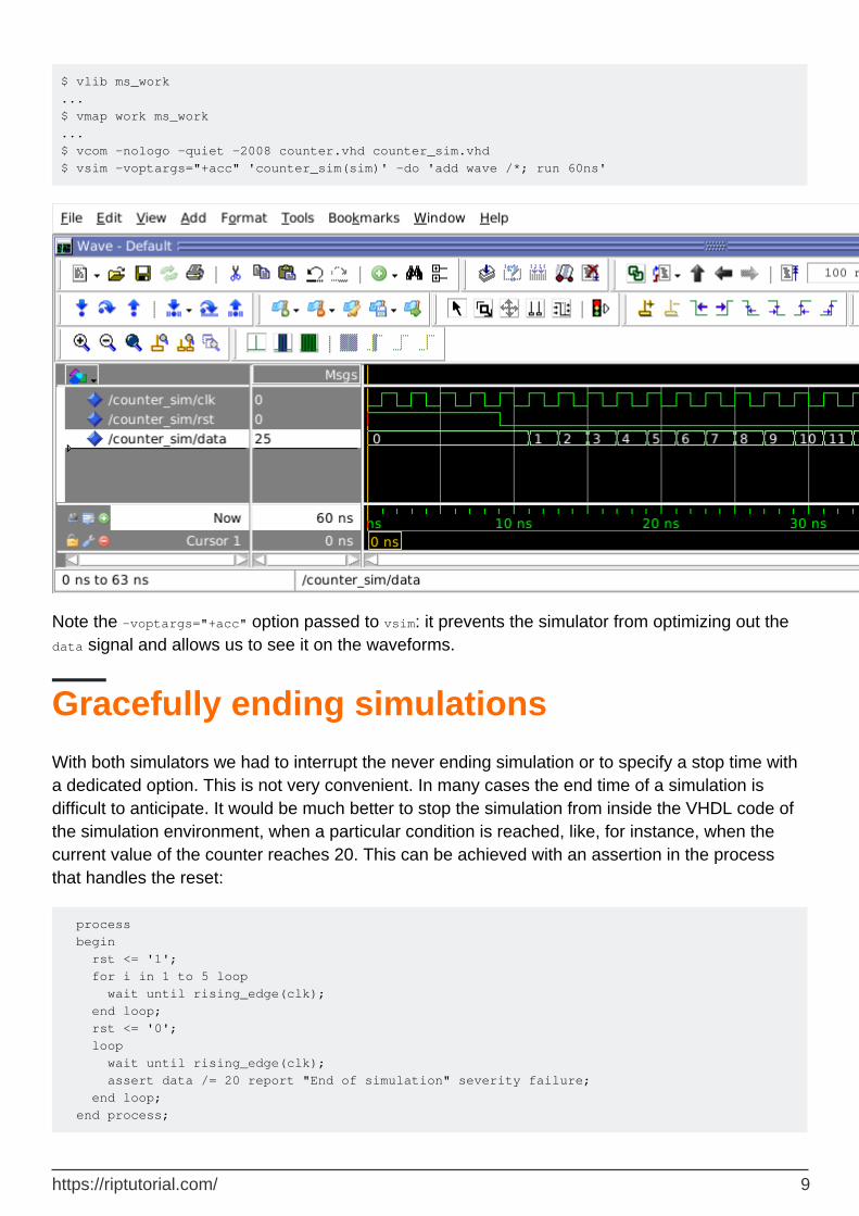
$ vlib ms_work ... $ vmap work ms_work ... $ vcom -nologo -quiet -2008 counter.vhd counter_sim.vhd $ vsim -voptargs="+acc" 'counter_sim(sim)' -do 'add wave /*; run 60ns'

Note the -voptargs="+acc" option passed to vsim: it prevents the simulator from optimizing out the data signal and allows us to see it on the waveforms.

Gracefully ending simulations

With both simulators we had to interrupt the never ending simulation or to specify a stop time with a dedicated option. This is not very convenient. In many cases the end time of a simulation is difficult to anticipate. It would be much better to stop the simulation from inside the VHDL code of the simulation environment, when a particular condition is reached, like, for instance, when the current value of the counter reaches 20. This can be achieved with an assertion in the process that handles the reset:

process begin rst <= '1'; for i in 1 to 5 loop wait until rising_edge(clk); end loop; rst <= '0'; loop wait until rising_edge(clk); assert data /= 20 report "End of simulation" severity failure; end loop; end process;


https://i.stack.imgur.com/xhAgo.png

As long as data is different from 20 the simulation continues. When data reaches 20, the simulation crashes with an error message:

$ ghdl -a --workdir=gh_work --std=08 counter_sim.vhd $ ghdl -r --workdir=gh_work --std=08 counter_sim sim counter_sim.vhd:90:24:@51ns:(assertion failure): End of simulation ghdl:error: assertion failed from: process work.counter_sim(sim2).P1 at counter_sim.vhd:90 ghdl:error: simulation failed

Note that we re-compiled only the simulation environment: it is the only design that changed and it is the top level. Had we modified only counter.vhd, we would have had to re-compile both: counter.vhd because it changed and counter_sim.vhd because it depends on counter.vhd.

Crashing the simulation with an error message is not very elegant. It can even be a problem when automatically parsing the simulation messages to decide if an automatic non-regression test passed or not. A better and much more elegant solution is to stop all processes when a condition is reached. This can be done, for instance, by adding a boolean End Of Simulation (eof) signal. By default it is initialized to false at the beginning of the simulation. One of our processes will set it to true when the time has come to end the simulation. All the other processes will monitor this signal and stop with an eternal wait when it will become true:

signal eos: boolean; ... process begin clk <= '0'; wait for 1 ns; clk <= '1'; wait for 1 ns; if eos then report "End of simulation"; wait; end if; end process; process begin rst <= '1'; for i in 1 to 5 loop wait until rising_edge(clk); end loop; rst <= '0'; for i in 1 to 20 loop wait until rising_edge(clk); end loop; eos <= true; wait; end process;

$ ghdl -a --workdir=gh_work --std=08 counter_sim.vhd $ ghdl -r --workdir=gh_work --std=08 counter_sim sim counter_sim.vhd:120:24:@50ns:(report note): End of simulation

Last but not least, there is an even better solution introduced in VHDL 2008 with the standard


package env and the stop and finish procedures it declares:

use std.env.all; ... process begin rst <= '1'; for i in 1 to 5 loop wait until rising_edge(clk); end loop; rst <= '0'; for i in 1 to 20 loop wait until rising_edge(clk); end loop; finish; end process;

$ ghdl -a --workdir=gh_work --std=08 counter_sim.vhd $ ghdl -r --workdir=gh_work --std=08 counter_sim sim simulation finished @49ns

Signals vs. variables, a brief overview of the simulation semantics of VHDL

This example deals with one of the most fundamental aspects of the VHDL language: the simulation semantics. It is intended for VHDL beginners and presents a simplified view where many details have been omitted (postponed processes, VHDL Procedural Interface, shared variables...) Readers interested in the real complete semantics shall refer to the Language Reference Manual (LRM).

Signals and variables

Most classical imperative programming languages use variables. They are value containers. An assignment operator is used to store a value in a variable:

a = 15;

and the value currently stored in a variable can be read and used in other statements:

if(a == 15) { print "Fifteen" }

VHDL also uses variables and they have exactly the same role as in most imperative languages. But VHDL also offers another kind of value container: the signal. Signals also store values, can also be assigned and read. The type of values that can be stored in signals is (almost) the same as in variables.

So, why having two kinds of value containers? The answer to this question is essential and at the heart of the language. Understanding the difference between variables and signals is the very first thing to do before trying to program anything in VHDL.


Let us illustrate this difference on a concrete example: the swapping.

Note: all the following code snippets are parts of processes. We will see later what processes are.

tmp := a; a := b; b := tmp;

swaps variables a and b. After executing these 3 instructions, the new content of a is the old content of b and conversely. Like in most programming languages, a third temporary variable (tmp) is needed. If, instead of variables, we wanted to swap signals, we would write:

r <= s; s <= r;

or:

s <= r; r <= s;

with the same result and without the need of a third temporary signal!

Note: the VHDL signal assignment operator <= is different from the variable assignment operator :=.

Let us look at a second example in which we assume that the print subprogram prints the decimal representation of its parameter. If a is an integer variable and its current value is 15, executing:

a := 2 * a; a := a - 5; a := a / 5; print(a);

will print:

5

If we execute this step by step in a debugger we can see the value of a changing from the initial 15 to 30, 25 and finally 5.

But if s is an integer signal and its current value is 15, executing:

s <= 2 * s; s <= s - 5; s <= s / 5; print(s); wait on s; print(s);


will print:

15 3

If we execute this step by step in a debugger we will not see any value change of s until after the wait instruction. Moreover, the final value of s will not be 15, 30, 25 or 5 but 3!

This apparently strange behavior is due the fundamentally parallel nature of digital hardware, as we will see in the following sections.

Parallelism

VHDL being a Hardware Description Language (HDL), it is parallel by nature. A VHDL program is a collection of sequential programs that run in parallel. These sequential programs are called processes:

P1: process begin instruction1; instruction2; ... instructionN; end process P1; P2: process begin ... end process P2;

The processes, just like the hardware they are modelling, never end: they are infinite loops. After executing the last instruction, the execution continues with the first.

As with any programming language that supports one form or another of parallelism, a scheduler is responsible for deciding which process to execute (and when) during a VHDL simulation. Moreover, the language offers specific constructs for inter-process communication and synchronization.

Scheduling

The scheduler maintains a list of all processes and, for each of them, records its current state which can be running, run-able or suspended. There is at most one process in running state: the one that is currently executed. As long as the currently running process does not execute a wait instruction, it continues running and prevents any other process from being executed. The VHDL scheduler is not preemptive: it is each process responsibility to suspend itself and let other processes run. This is one of the problems that VHDL beginners frequently encounter: the free running process.


P3: process variable a: integer; begin a := s; a := 2 * a; r <= a; end process P3;

Note: variable a is declared locally while signals s and r are declared elsewhere, at a higher level. VHDL variables are local to the process that declares them and cannot be seen by other processes. Another process could also declare a variable named a, it would not be the same variable as the one of process P3.

As soon as the scheduler will resume the P3 process, the simulation will get stuck, the simulation current time will not progress anymore and the only way to stop this will be to kill or interrupt the simulation. The reason is that P3 has not wait statement and will thus stay in running state forever, looping over its 3 instructions. No other process will ever be given a chance to run, even if it is run-able.

Even processes containing a wait statement can cause the same problem:

P4: process variable a: integer; begin a := s; a := 2 * a; if a = 16 then wait on s; end if; r <= a; end process P4;

Note: the VHDL equality operator is =.

If process P4 is resumed while the value of signal s is 3, it will run forever because the a = 16 condition will never be true.

Let us assume that our VHDL program does not contain such pathological processes. When the running process executes a wait instruction, it is immediately suspended and the scheduler puts it in the suspended state. The wait instruction also carries the condition for the process to become run-able again. Example:

wait on s;

means suspend me until the value of signal s changes. This condition is recorded by the scheduler. The scheduler then selects another process among the run-able, puts it in running state and executes it. And the same repeats until all run-able processes have been executed and suspended.

Important note: when several processes are run-able, the VHDL standard does not specify how the scheduler shall select which one to run. A consequence is that,


depending on the simulator, the simulator's version, the operating system, or anything else, two simulations of the same VHDL model could, at one point, make different choices and select a different process to execute. If this choice had an impact on the simulation results, we could say that VHDL is non-deterministic. As non-determinism is usually undesirable, it would be the responsibility of the programmers to avoid non-deterministic situations. Fortunately, VHDL takes care of this and this is where signals enter the picture.

Signals and inter-process communication

VHDL avoids non determinism using two specific characteristics:

Processes can exchange information only through signals1.

signal r, s: integer; -- Common to all processes ... P5: process variable a: integer; -- Different from variable a of process P6 begin a := s + 1; r <= a; a := r + 1; wait on s; end process P5; P6: process variable a: integer; -- Different from variable a of process P5 begin a := r + 1; s <= a; wait on r; end process P6;

Note: VHDL comments extend from -- to the end of the line.

The value of a VHDL signal does not change during the execution of processes2.

Every time a signal is assigned, the assigned value is recorded by the scheduler but the current value of the signal remains unchanged. This is another major difference with variables that take their new value immediately after being assigned.

Let us look at an execution of process P5 above and assume that a=5, s=1 and r=0 when it is resumed by the scheduler. After executing instruction a := s + 1;, the value of variable a changes and becomes 2 (1+1). When executing the next instruction r <= a; it is the new value of a (2) that is assigned to r. But r being a signal, the current value of r is still 0. So, when executing a := r + 1;, variable a takes (immediately) value 1 (0+1), not 3 (2+1) as the intuition would say.

When will signal r really take its new value? When the scheduler will have executed all run-able processes and they will all be suspended. This is also referred to as: after one delta cycle. It is only then that the scheduler will look at all the values that have been assigned to signals and actually update the values of the signals. A VHDL simulation is an alternation of execution phases


and signal update phases. During execution phases, the value of the signals is frozen. Symbolically, we say that between an execution phase and the following signal update phase a delta of time elapsed. This is not real time. A delta cycle has no physical duration.

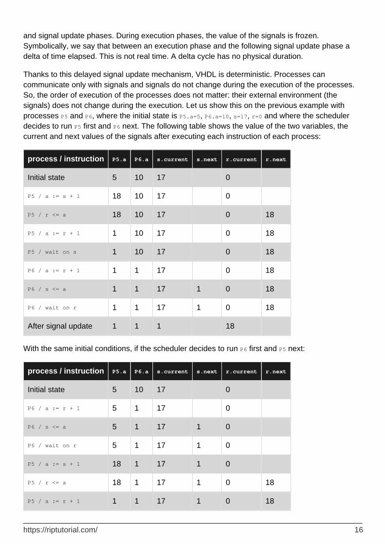
Thanks to this delayed signal update mechanism, VHDL is deterministic. Processes can communicate only with signals and signals do not change during the execution of the processes. So, the order of execution of the processes does not matter: their external environment (the signals) does not change during the execution. Let us show this on the previous example with processes P5 and P6, where the initial state is P5.a=5, P6.a=10, s=17, r=0 and where the scheduler decides to run P5 first and P6 next. The following table shows the value of the two variables, the current and next values of the signals after executing each instruction of each process:

process / instruction P5.a P6.a s.current s.next r.current r.next

Initial state 5 10 17 0

P5 / a := s + 1 18 10 17 0

P5 / r <= a 18 10 17 0 18

P5 / a := r + 1 1 10 17 0 18

P5 / wait on s 1 10 17 0 18

P6 / a := r + 1 1 1 17 0 18

P6 / s <= a 1 1 17 1 0 18

P6 / wait on r 1 1 17 1 0 18

After signal update 1 1 1 18

With the same initial conditions, if the scheduler decides to run P6 first and P5 next:


Initial state 5 10 17 0

P6 / a := r + 1 5 1 17 0

P6 / s <= a 5 1 17 1 0

P6 / wait on r 5 1 17 1 0

P5 / a := s + 1 18 1 17 1 0

P5 / r <= a 18 1 17 1 0 18

P5 / a := r + 1 1 1 17 1 0 18



P5 / wait on s 1 1 17 1 0 18

After signal update 1 1 1 18

As we can see, after the execution of our two processes, the result is the same whatever the order of execution.

This counter-intuitive signal assignment semantics is the reason of a second type of problems that VHDL beginners frequently encounter: the assignment that apparently does not work because it is delayed by one delta cycle. When running process P5 step-by-step in a debugger, after r has been assigned 18 and a has been assigned r + 1, one could expect that the value of a is 19 but the debugger obstinately says that r=0 and a=1...

Note: the same signal can be assigned several times during the same execution phase. In this case, it is the last assignment that decides the next value of the signal. The other assignments have no effect at all, just like if they never had been executed.

It is time to check our understanding: please go back to our very first swapping example and try to understand why:

process begin --- s <= r; r <= s; --- end process;

actually swaps signals r and s without the need of a third temporary signal and why:

process begin --- r <= s; s <= r; --- end process;

would be strictly equivalent. Try to understand also why, if s is an integer signal and its current value is 15, and we execute:

process begin --- s <= 2 * s; s <= s - 5; s <= s / 5; print(s); wait on s; print(s); ---


end process;

the two first assignments of signal s have no effect, why s is finally assigned 3 and why the two printed values are 15 and 3.

Physical time

In order to model hardware it is very useful to be able to model the physical time taken by some operation. Here is an example of how this can be done in VHDL. The example models a synchronous counter and it is a full, self-contained, VHDL code that could be compiled and simulated:

-- File counter.vhd entity counter is end entity counter; architecture arc of counter is signal clk: bit; -- Type bit has two values: '0' and '1' signal c, nc: natural; -- Natural (non-negative) integers begin P1: process begin clk <= '0'; wait for 10 ns; -- Ten nano-seconds delay clk <= '1'; wait for 10 ns; -- Ten nano-seconds delay end process P1; P2: process begin if clk = '1' and clk'event then c <= nc; end if; wait on clk; end process P2; P3: process begin nc <= c + 1 after 5 ns; -- Five nano-seconds delay wait on c; end process P3; end architecture arc;

In process P1 the wait instruction is not used to wait until the value of a signal changes, like we saw up to now, but to wait for a given duration. This process models a clock generator. Signal clk is the clock of our system, it is periodic with period 20 ns (50 MHz) and has duty cycle.

Process P2 models a register that, if a rising edge of clk just occurred, assigns the value of its input nc to its output c and then waits for the next value change of clk.

Process P3 models an incrementer that assigns the value of its input c, incremented by one, to its output nc... with a physical delay of 5 ns. It then waits until the value of its input c changes. This is also new. Up to now we always assigned signals with:


s <= value;

which, for the reasons explained in the previous sections, we can implicitly translate into:

s <= value; -- after delta

This small digital hardware system could be represented by the following figure:

With the introduction of the physical time, and knowing that we also have a symbolic time measured in delta, we now have a two dimensional time that we will denote T+D where T is a physical time measured in nano-seconds and D a number of deltas (with no physical duration).

The complete picture

There is one important aspect of the VHDL simulation that we did not discuss yet: after an execution phase all processes are in suspended state. We informally stated that the scheduler then updates the values of the signals that have been assigned. But, in our example of a synchronous counter, shall it update signals clk, c and nc at the same time? What about the physical delays? And what happens next with all processes in suspended state and none in run-able state?

The complete (but simplified) simulation algorithm is the following:

InitializationSet current time Tc to 0+0 (0 ns, 0 delta-cycle)•Initialize all signals.•Execute each process until it suspends on a wait statement.

Record the values and delays of signal assignments.○

Record the conditions for the process to resume (delay or signal change).○

•

Compute the next time Tn as the earliest of:The resume time of processes suspended by a wait for <delay>.○

The next time at which a signal value shall change.○

•

1.

Simulation cycleTc=Tn.•Update signals that need to be.•Put in run-able state all processes that were waiting for a value change of one of the signals that has been updated.

•

Put in run-able state all processes that were suspended by a wait for <delay> •

2.


https://i.stack.imgur.com/0Lcry.png

statement and for which the resume time is Tc.Execute all run-able processes until they suspend.

Record the values and delays of signal assignments.○

Record the conditions for the process to resume (delay or signal change).○

•

Compute the next time Tn as the earliest of:The resume time of processes suspended by a wait for <delay>.○

The next time at which a signal value shall change.○

•

If Tn is infinity, stop simulation. Else, start a new simulation cycle.•

Manual simulation

To conclude, let us now manually exercise the simplified simulation algorithm on the synchronous counter presented above. We arbitrary decide that, when several processes are run-able, the order will be P3>P2>P1. The following tables represent the evolution of the state of the system during the initialization and the first simulation cycles. Each signal has its own column in which the current value is indicated. When a signal assignment is executed, the scheduled value is appended to the current value, e.g. a/b@T+D if the current value is a and the next value will be b at time T+D (physical time plus delta cycles). The 3 last columns indicate the condition to resume the suspended processes (name of signals that must change or time at which the process shall resume).

Initialization phase:

Operations Tc Tn clk c nc P1 P2 P3

Set current time 0+0

Initialize all signals 0+0 '0' 0 0

P3/nc<=c+1 after 5 ns 0+0 '0' 0 0/1@5+0

P3/wait on c 0+0 '0' 0 0/1@5+0 c

P2/if clk='1'... 0+0 '0' 0 0/1@5+0 c

P2/end if 0+0 '0' 0 0/1@5+0 c

P2/wait on clk 0+0 '0' 0 0/1@5+0 clk c

P1/clk<='0' 0+0 '0'/'0'@0+1 0 0/1@5+0 clk c

P1/wait for 10 ns 0+0 '0'/'0'@0+1 0 0/1@5+0 10+0 clk c

Compute next time 0+0 0+1 '0'/'0'@0+1 0 0/1@5+0 10+0 clk c


Simulation cycle #1


Set current time 0+1 '0'/'0'@0+1 0 0/1@5+0 10+0 clk c

Update signals 0+1 '0' 0 0/1@5+0 10+0 clk c

Compute next time 0+1 5+0 '0' 0 0/1@5+0 10+0 clk c

Note: during the first simulation cycle there is no execution phase because none of our 3 processes has its resume condition satisfied. P2 is waiting for a value change of clk and there has been a transaction on clk, but as the old and new values are the same, this is not a value change.

Simulation cycle #2


Set current time 5+0 '0' 0 0/1@5+0 10+0 clk c

Update signals 5+0 '0' 0 1 10+0 clk c

Compute next time 5+0 10+0 '0' 0 1 10+0 clk c

Note: again, there is no execution phase. nc changed but no process is waiting on nc.

Simulation cycle #3


Set current time 10+0 '0' 0 1 10+0 clk c


P1/clk<='1' 10+0 '0'/'1'@10+1 0 1 clk c

P1/wait for 10 ns 10+0 '0'/'1'@10+1 0 1 20+0 clk c

Compute next time 10+0 10+1 '0'/'1'@10+1 0 1 20+0 clk c

Simulation cycle #4



Set current time 10+1 '0'/'1'@10+1 0 1 20+0 clk c


P2/if clk='1'... 10+1 '1' 0 1 20+0 c

P2/c<=nc 10+1 '1' 0/1@10+2 1 20+0 c

P2/end if 10+1 '1' 0/1@10+2 1 20+0 c

P2/wait on clk 10+1 '1' 0/1@10+2 1 20+0 clk c

Compute next time 10+1 10+2 '1' 0/1@10+2 1 20+0 clk c

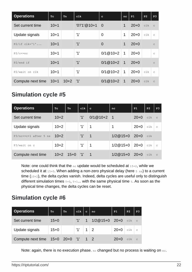
Simulation cycle #5


Set current time 10+2 '1' 0/1@10+2 1 20+0 clk c


P3/nc<=c+1 after 5 ns 10+2 '1' 1 1/2@15+0 20+0 clk

P3/wait on c 10+2 '1' 1 1/2@15+0 20+0 clk c


Note: one could think that the nc update would be scheduled at 15+2, while we scheduled it at 15+0. When adding a non-zero physical delay (here 5 ns) to a current time (10+2), the delta cycles vanish. Indeed, delta cycles are useful only to distinguish different simulation times T+0, T+1... with the same physical time T. As soon as the physical time changes, the delta cycles can be reset.

Simulation cycle #6


Set current time 15+0 '1' 1 1/2@15+0 20+0 clk c



Note: again, there is no execution phase. nc changed but no process is waiting on nc.


Simulation cycle #7




P1/clk<='0' 20+0 '1'/'0'@20+1 1 2 clk c

P1/wait for 10 ns 20+0 '1'/'0'@20+1 1 2 30+0 clk c


Simulation cycle #8




P2/if clk='1'... 20+1 '0' 1 2 30+0 c

P2/end if 20+1 '0' 1 2 30+0 c

P2/wait on clk 20+1 '0' 1 2 30+0 clk c


Simulation cycle #9




P1/clk<='1' 30+0 '0'/'1'@30+1 1 2 clk c

P1/wait for 10 ns 30+0 '0'/'1'@30+1 1 2 40+0 clk c


Simulation cycle #10





P2/if clk='1'... 30+1 '1' 1 2 40+0 c

P2/c<=nc 30+1 '1' 1/2@30+2 2 40+0 c

P2/end if 30+1 '1' 1/2@30+2 2 40+0 c

P2/wait on clk 30+1 '1' 1/2@30+2 2 40+0 clk c

Compute next time 30+1 30+2 '1' 1/2@30+2 2 40+0 clk c

Simulation cycle #11


Set current time 30+2 '1' 1/2@30+2 2 40+0 clk c


P3/nc<=c+1 after 5 ns 30+2 '1' 2 2/3@35+0 40+0 clk

P3/wait on c 30+2 '1' 2 2/3@35+0 40+0 clk c


Read Getting started with vhdl online: https://riptutorial.com/vhdl/topic/3803/getting-started-with-vhdl


https://riptutorial.com/vhdl/topic/3803/getting-started-with-vhdl

https://riptutorial.com/vhdl/topic/3803/getting-started-with-vhdl

Chapter 2: Comments

Introduction

Any decent programming language supports comments. In VHDL they are especially important because understanding a VHDL code, even moderately sophisticated, is frequently challenging.

Examples

Single line comments

A single line comment starts with two hyphens (--) and extends up to the end of the line. Example :

-- This process models the state register process(clock, aresetn) begin if aresetn = '0' then -- Active low, asynchronous reset state <= IDLE; elsif rising_edge(clock) then -- Synchronized on the rising edge of the clock state <= next_state; end if; end process;

Delimited comments

Starting with VHDL 2008, a comment can also extend on several lines. Multi-lines comments start with /* and end with */. Example :

/* This process models the state register. It has an active low, asynchronous reset and is synchronized on the rising edge of the clock. */ process(clock, aresetn) begin if aresetn = '0' then state <= IDLE; elsif rising_edge(clock) then state <= next_state; end if; end process;

Delimited comments can also be used on less than a line:

-- Finally, we decided to skip the reset... process(clock/*, aresetn*/) begin /*if aresetn = '0' then state <= IDLE; els*/if rising_edge(clock) then


state <= next_state; end if; end process;

Nested comments

Starting a new comment (single line or delimited) inside a comment (single line or delimited) has no effect and is ignored. Examples:

-- This is a single-line comment. This second -- has no special meaning. -- This is a single-line comment. This /* has no special meaning. /* This is not a single-line comment. And this -- has no special meaning. */ /* This is not a single-line comment. And this second /* has no special meaning. */

Read Comments online: https://riptutorial.com/vhdl/topic/9292/comments


https://riptutorial.com/vhdl/topic/9292/comments

Chapter 3: D-Flip-Flops (DFF) and latches

Remarks

D-Flip-Flops (DFF) and latches are memory elements. A DFF samples its input on one or the other edge of its clock (not both) while a latch is transparent on one level of its enable and memorizing on the other. The following figure illustrates the difference:

Modelling DFFs or latches in VHDL is easy but there are a few important aspects that must be taken into account:

The differences between VHDL models of DFFs and latches.•

How to describe the edges of a signal.•

How to describe synchronous or asynchronous set or resets.•

Examples

D-Flip-Flops (DFF)

In all examples:

clk is the clock,•d is the input,•q is the output,•srst is an active high synchronous reset,•srstn is an active low synchronous reset,•


https://i.stack.imgur.com/nkCvj.png

arst is an active high asynchronous reset,•arstn is an active low asynchronous reset,•sset is an active high synchronous set,•ssetn is an active low synchronous set,•aset is an active high asynchronous set,•asetn is an active low asynchronous set•

All signals are of type ieee.std_logic_1164.std_ulogic. The syntax used is the one that leads to correct synthesis results with all logic synthesizers. Please see the Clock edge detection example for a discussion about alternate syntax.

Rising edge clock

process(clk) begin if rising_edge(clk) then q <= d; end if; end process;

Falling edge clock

process(clk) begin if falling_edge(clk) then q <= d; end if; end process;

Rising edge clock, synchronous active high reset

process(clk) begin if rising_edge(clk) then if srst = '1' then q <= '0'; else q <= d; end if; end if; end process;

Rising edge clock, asynchronous active high


reset

process(clk, arst) begin if arst = '1' then q <= '0'; elsif rising_edge(clk) then q <= d; end if; end process;

Falling edge clock, asynchronous active low reset, synchronous active high set

process(clk, arstn) begin if arstn = '0' then q <= '0'; elsif falling_edge(clk) then if sset = '1' then q <= '1'; else q <= d; end if; end if; end process;

Rising edge clock, asynchronous active high reset, asynchronous active low set

Note: set has higher priority than reset

process(clk, arst, asetn) begin if asetn = '0' then q <= '1'; elsif arst = '1' then q <= '0'; elsif rising_edge(clk) then q <= d; end if; end process;

Latches

In all examples:


en is the enable signal,•d is the input,•q is the output,•srst is an active high synchronous reset,•srstn is an active low synchronous reset,•arst is an active high asynchronous reset,•arstn is an active low asynchronous reset,•sset is an active high synchronous set,•ssetn is an active low synchronous set,•aset is an active high asynchronous set,•asetn is an active low asynchronous set•

All signals are of type ieee.std_logic_1164.std_ulogic. The syntax used is the one that leads to correct synthesis results with all logic synthesizers. Please see the Clock edge detection example for a discussion about alternate syntax.

Active high enable

process(en, d) begin if en = '1' then q <= d; end if; end process;

Active low enable

process(en, d) begin if en = '0' then q <= d; end if; end process;

Active high enable, synchronous active high reset

process(en, d) begin if en = '1' then if srst = '1' then q <= '0'; else q <= d; end if;


end if; end process;

Active high enable, asynchronous active high reset

process(en, d, arst) begin if arst = '1' then q <= '0'; elsif en = '1' then q <= d; end if; end process;

Active low enable, asynchronous active low reset, synchronous active high set

process(en, d, arstn) begin if arstn = '0' then q <= '0'; elsif en = '0' then if sset = '1' then q <= '1'; else q <= d; end if; end if; end process;

Active high enable, asynchronous active high reset, asynchronous active low set

Note: set has higher priority than reset

process(en, d, arst, asetn) begin if asetn = '0' then q <= '1'; elsif arst = '1' then q <= '0'; elsif en = '1' then q <= d; end if; end process;


Clock edge detection

The short story

Whith VHDL 2008 and if the type of the clock is bit, boolean, ieee.std_logic_1164.std_ulogic or ieee.std_logic_1164.std_logic, a clock edge detection can be coded for rising edge

if rising_edge(clock) then•if clock'event and clock = '1' then -- type bit, std_ulogic or std_logic•if clock'event and clock then -- type boolean•

and for falling edge

if falling_edge(clock) then•if clock'event and clock = '0' then -- type bit, std_ulogic or std_logic•if clock'event and not clock then -- type boolean•

This will behave as expected, both for simulation and synthesis.

Note: the definition of a rising edge on a signal of type std_ulogic is a bit more complex than the simple if clock'event and clock = '1' then. The standard rising_edge function, for instance, has a different definition. Even if it will probably make no difference for synthesis, it could make one for simulation.

The use of the rising_edge and falling_edge standard functions is strongly encouraged. With previous versions of VHDL the use of these functions may require to explicitly declare the use of standard packages (e.g. ieee.numeric_bit for type bit) or even to define them in a custom package.

Note: do not use the rising_edge and falling_edge standard functions to detect edges of non-clock signals. Some synthesizers could conclude that the signal is a clock. Hint: detecting an edge on a non-clock signal can frequently be done by sampling the signal in a shift register and comparing the sampled values at different stages of the shift register.

The long story

Properly describing the detection of the edges of a clock signal is essential when modelling D-Flip-Flops (DFF). An edge is, by definition, a transition from one particular value to another. For instance, we can defined the rising edge of a signal of type bit (the standard VHDL enumerated type that takes two values: '0' and '1') as the transition from '0' to '1'. For type boolean we can define it as a transition from false to true.

Frequently, more complex types are used. The ieee.std_logic_1164.std_ulogic type, for instance, is also an enumerated type, just like bit or boolean, but it has 9 values instead of 2:


Value Meaning

'U' Uninitialized

'X' Forcing unknown

'0' Forcing low level

'1' Forcing high level

'Z' High impedance

'W' Weak unknown

'L' Weak low level

'H' Weak high level

'-' Don't care

Defining a rising edge on such a type is a bit more complex than for bit or boolean. We can, for instance, decide that it is a transition from '0' to '1'. But we can also decide that it is a transition from '0' or 'L' to '1' or 'H'.

Note: it is this second definition that the standard uses for the rising_edge(signal s: std_ulogic) function defined in ieee.std_logic_1164.

When discussing the various ways to detect edges, it is thus important to consider the type of the signal. It is also important to take the modeling goal into account: simulation only or logic synthesis? Let us illustrate this on a few examples:

Rising edge DFF with type bit

signal clock, d, q: bit; ... P1: process(clock) begin if clock = '1' then q <= d; end if; end process P1;

Technically, on a pure simulation semantics point of view, process P1 models a rising edge triggered DFF. Indeed, the q <= d assignment is executed if and only if:

clock changed (this is what the sensitivity list expresses) and•the current value of clock is '1'.•

As clock is of type bit and type bit has only values '0' and '1', this is exactly what we defined as a rising edge of a signal of type bit. Any simulator will handle this model as we expect.


Note: For logic synthesizers, things are a bit more complex, as we will see later.

Rising edge DFF with asynchronous active high reset and type bit

In order to add an asynchronous active high reset to our DFF, one could try something like:

signal clock, reset, d, q: bit; ... P2_BOGUS: process(clock, reset) begin if reset = '1' then q <= '0'; elsif clock = '1' then q <= d; end if; end process P2_BOGUS;

But this does not work. The condition for the q <= d assignment to be executed should be: a rising edge of clock while reset = '0'. But what we modeled is:

clock or reset or both changed and•reset = '0' and•clock = '1'•

Which is not the same: if reset changes from '1' to '0' while clock = '1' the assignment will be executed while it is not a rising edge of clock.

In fact, there is no way to model this in VHDL without the help of a signal attribute:

P2_OK: process(clock, reset) begin if reset = '1' then q <= '0'; elsif clock = '1' and clock'event then q <= d; end if; end process P2_OK;

The clock'event is the signal attribute event applied to signal clock. It evaluates as a boolean and it is true if and only if signal clock changed during the signal update phase that just preceded the current execution phase. Thanks to this, process P2_OK now perfectly models what we want in simulation (and synthesis).

Synthesis semantics

Many logic synthesizers identify signal edge detections based on syntactic patterns, not on the semantics of the VHDL model. In other words, they consider what the VHDL code looks like, not what behavior it models. One of the patterns they all recognize is:


if clock = '1' and clock'event then

So, even in the example of process P1 we should use it if we want our model to be synthesizable by all logic synthesizers:

signal clock, d, q: bit; ... P1_OK: process(clock) begin if clock = '1' and clock'event then q <= d; end if; end process P1_OK;

The and clock'event part of the condition is completely redundant with the sensitivity list but as some synthesizers need it...

Rising edge DFF with asynchronous active high reset and type std_ulogic

In this case, expressing the rising edge of the clock and the reset condition can become complicated. If we retain the definition of a rising edge that we proposed above and if we consider that the reset is active if it is '1' or 'H', the model becomes:

library ieee; use ieee.std_logic_1164.all; ... signal clock, reset, d, q: std_ulogic; ... P4: process(clock, reset) begin if reset = '1' or reset = 'H' then q <= '0'; elsif clock'event and (clock'last_value = '0' or clock'last_value = 'L') and (clock = '1' or clock = 'H') then q <= d; end if; end process P4;

Note: 'last_value is another signal attribute that returns the value the signal had before the last value change.

Helper functions

The VHDL 2008 standard offers several helper functions to simplify the detection of signal edges, especially with multi-valued enumerated types like std_ulogic. The std.standard package defines the rising_edge and falling_edge functions on types bit and boolean and the ieee.std_logic_1164 package defines them on types std_ulogic and std_logic.


Note: with previous versions of VHDL the use of these functions may require to explicitly declare the use of standard packages (e.g. ieee.numeric_bit for type bit) or even to define them in a user package.

Let us revisit the previous examples and use the helper functions:

signal clock, d, q: bit; ... P1_OK_NEW: process(clock) begin if rising_edge(clock) then q <= d; end if; end process P1_OK_NEW;

signal clock, d, q: bit; ... P2_OK_NEW: process(clock, reset) begin if reset = '1' then q <= '0'; elsif rising_edge(clock) then q <= d; end if; end process P2_OK_NEW;

library ieee; use ieee.std_logic_1164.all; ... signal clock, reset, d, q: std_ulogic; ... P4_NEW: process(clock, reset) begin if reset = '1' then q <= '0'; elsif rising_edge(clock) then q <= d; end if; end process P4_NEW;

Note: in this last example we also simplified the test on the reset. Floating, high impedance, resets are quite rare and, in most cases, this simplified version works for simulation and synthesis.

Read D-Flip-Flops (DFF) and latches online: https://riptutorial.com/vhdl/topic/5983/d-flip-flops--dff--and-latches


https://riptutorial.com/vhdl/topic/5983/d-flip-flops--dff--and-latches

https://riptutorial.com/vhdl/topic/5983/d-flip-flops--dff--and-latches

Chapter 4: Digital hardware design using VHDL in a nutshell

Introduction

In this topic we propose a simple method to correctly design simple digital circuits with VHDL. The method is based on graphical block diagrams and an easy-to-remember principle:

Think hardware first, code VHDL next

It is intended for beginners in digital hardware design using VHDL, with a limited understanding of the synthesis semantics of the language.

Remarks

Digital hardware design using VHDL is simple, even for beginners, but there are a few important things to know and a small set of rules to obey. The tool used to transform a VHDL description in digital hardware is a logic synthesizer. The semantics of the VHDL language used by logic synthesizers is rather different from the simulation semantics described in the Language Reference Manual (LRM). Even worse: it is not standardized and varies between synthesis tools.

The proposed method introduces several important limitations for the sake of simplicity:

No level-triggered latches.•The circuits are synchronous on the rising edge of a single clock.•No asynchronous reset or set.•No multiple drive on resolved signals.•

The Block diagram example, first of a series of 3, briefly presents the basics of digital hardware and proposes a short list of rules to design a block diagram of a digital circuit. The rules help to guarantee a straightforward translation to VHDL code that simulates and synthesizes as expected.

The Coding example explains the translation from a block diagram to VHDL code and illustrates it on a simple digital circuit.

Finally, the John Cooley’s design contest example shows how to apply the proposed method on a more complex example of digital circuit. It also elaborates on the introduced limitations and relaxes some of them.

Examples

Block diagram

Digital hardware is built from two types of hardware primitives:


http://www.riptutorial.com/vhdl/example/19653/block-diagram

http://www.riptutorial.com/vhdl/example/19654/coding

http://www.riptutorial.com/vhdl/example/19655/john-cooley-s-design-contest

Combinatorial gates (inverters, and, or, xor, 1-bit full adders, 1-bit multiplexers...) These logic gates perform a simple boolean computation on their inputs and produce an output. Each time one of their inputs changes, they start propagating electrical signals and, after a short delay, the output stabilizes to the resulting value. The propagation delay is important because it is strongly related to the speed at which the digital circuit can run, that is, its maximum clock frequency.

•

Memory elements (latches, D-flip-flops, RAMs...). Contrary to the combinatorial logic gates, memory elements do not react immediately to the change of any of their inputs. They have data inputs, control inputs and data outputs. They react on a particular combination of control inputs, not on any change of their data inputs. The rising-edge triggered D-flip-flop (DFF), for instance, has a clock input and a data input. On every rising edge of the clock, the data input is sampled and copied to the data output that remains stable until the next rising edge of the clock, even if the data input changes in between.

•

A digital hardware circuit is a combination of combinatorial logic and memory elements. Memory elements have several roles. One of them is to allow reusing the same combinatorial logic for several consecutive operations on different data. Circuits using this are frequently referred to as sequential circuits. The figure below shows an example of a sequential circuit that accumulates integer values using the same combinatorial adder, thanks to a rising-edge triggered register. It is also our first example of a block diagram.

Pipe-lining is another common use of memory elements and the basis of many micro-processor architectures. It aims at increasing the clock frequency of a circuit by splitting a complex processing in a succession of simpler operations, and at parallelizing the execution of several consecutive processing:

The block diagram is a graphical representation of the digital circuit. It helps making the right decisions and getting a good understanding of the overall structure before coding. It is the


https://i.stack.imgur.com/N5kaF.png

https://i.stack.imgur.com/ibrVX.png

equivalent of the recommended preliminary analysis phases in many software design methods. Experienced designers frequently skip this design phase, at least for simple circuits. If you are a beginner in digital hardware design, however, and if you want to code a digital circuit in VHDL, adopting the 10 simple rules below to draw your block diagram should help you getting it right:

Surround your drawing with a large rectangle. This is the boundary of your circuit. Everything that crosses this boundary is an input or output port. The VHDL entity will describe this boundary.

1.

Clearly separate edge-triggered registers (e.g. square blocks) from combinatorial logic (e.g. round blocks). In VHDL they will be translated into processes but of two very different kinds: synchronous and combinatorial.

2.

Do not use level-triggered latches, use only rising-edge triggered registers. This constraint does not come from VHDL, which is perfectly usable to model latches. It is just a reasonable advice for beginners. Latches are less frequently needed and their use poses many problems which we should probably avoid, at least for our first designs.

3.

Use the same single clock for all of your rising-edge triggered registers. There again, this constraint is here for the sake of simplicity. It does not come from VHDL, which is perfectly usable to model multi-clock systems. Name the clock clock. It comes from the outside and is an input of all square blocks and only them. If you wish, do not even represent the clock, it is the same for all square blocks and you can leave it implicit in your diagram.

4.

Represent the communications between blocks with named and oriented arrows. For the block an arrow comes from, the arrow is an output. For the block an arrow goes to, the arrow is an input. All these arrows will become ports of the VHDL entity, if they are crossing the large rectangle, or signals of the VHDL architecture.

5.

Arrows have one single origin but they can have several destinations. Indeed, if an arrow had several origins we would create a VHDL signal with several drivers. This is not completely impossible but requires special care in order to avoid short-circuits. We will thus avoid this for now. If an arrow has several destinations, fork the arrow as many times as needed. Use dots to distinguish connected and non-connected crossings.

6.

Some arrows come from outside the large rectangle. These are the input ports of the entity. An input arrow cannot also be the output of any of your blocks. This is enforced by the VHDL language: the input ports of an entity can be read but not written. This is again to avoid short-circuits.

7.

Some arrows go outside. These are the output ports. In VHDL versions prior 2008 the output ports of an entity can be written but not read. An output arrow must thus have one single origin and one single destination: the outside. No forks on output arrows, an output arrow cannot be also the input of one of your blocks. If you want to use an output arrow as an input for some of your blocks, insert a new round block to split it in two parts: the internal one, with as many forks as you wish, and the output arrow that comes from the new block and goes outside. The new block will become a simple continuous assignment in VHDL. A kind of transparent renaming. Since VHDL 2008 ouptut ports can also be read.

8.

All arrows that do not come or go from/to the outside are internal signals. You will declare them all in the VHDL architecture.

9.

Every cycle in the diagram must comprise at least one square block. This is not due to VHDL. It comes from the basic principles of digital hardware design. Combinatorial loops shall absolutely be avoided. Except in very rare cases, they do not produce any useful result. And a cycle of the block diagram that would comprise only round blocks would be a

10.


combinatorial loop.

Do not forget to carefully check the last rule, it is as essential as the others but it may be a bit more difficult to verify.

Unless you absolutely need features that we excluded for now, like latches, multiple-clocks or signals with multiple drivers, you should easily draw a block diagram of your circuit that complies with the 10 rules. If not, the problem is probably with the circuit you want, not with VHDL or the logic synthesizer. And it probably means that the circuit you want is not digital hardware.

Applying the 10 rules to our example of a sequential circuit would lead to a block diagram like:

The large rectangle around the diagram is crossed by 3 arrows, representing the input and output ports of the VHDL entity.

1.

The block diagram has two round (combinatorial) blocks - the adder and the output renaming block - and one square (synchronous) block - the register.

2.

It uses only edge-triggered registers.3. There is only one clock, named clock and we use only its rising edge.4. The block diagram has five arrows, one with a fork. They correspond to two internal signals, two input ports and one output port.

5.

All arrows have one origin and one destination except the arrow named Sum that has two destinations.

6.

The Data_in and Clock arrows are our two input ports. They are not output of our own blocks.7. The Data_out arrow is our output port. In order to be compatible with VHDL versions prior 2008, we added an extra renaming (round) block between Sum and Data_out. So, Data_out has exactly one source and one destination.

8.

Sum and Next_sum are our two internal signals.9. There is exactly one cycle in the graph and it comprises one square block.10.

Our block diagram complies with the 10 rules. The Coding example will detail how to translate this type of block diagrams in VHDL.

Coding

This example is the second of a series of 3. If you didn't yet, please read the Block diagram example first.

With a block diagram that complies with the 10 rules (see the Block diagram example), the VHDL coding becomes straightforward:


https://i.stack.imgur.com/TEv1Y.png




the large surrounding rectangle becomes the VHDL entity,•internal arrows become VHDL signals and are declared in the architecture,•every square block becomes a synchronous process in the architecture body,•every round block becomes a combinatorial process in the architecture body.•

Let us illustrate this on the block diagram of a sequential circuit:

The VHDL model of a circuit comprises two compilation units:

The entity that describes the circuit's name and its interface (ports names, directions and types). It is a direct translation of the large surrounding rectangle of the block diagram. Assuming the data are integers, and the clock uses the VHDL type bit (two values only: '0' and '1'), the entity of our sequential circuit could be:

•

entity sequential_circuit is port( Data_in: in integer; Clock: in bit; Data_out: out integer ); end entity sequential_circuit;

The architecture that describes the internals of the circuit (what it does). This is where the internal signals are declared and where all processes are instantiated. The skeleton of the architecture of our sequential circuit could be:

•

architecture ten_rules of sequential_circuit is signal Sum, Next_sum: integer; begin <...processes...> end architecture ten_rules;

We have three processes to add to the architecture body, one synchronous (square block) and two combinatorial (round blocks).

A synchronous process looks like this:

process(clock) begin if rising_edge(clock) then o1 <= i1; ... ox <= ix;


https://i.stack.imgur.com/TEv1Y.png

end if; end process;

where i1, i2,..., ix are all arrows that enter the corresponding square block of the diagram and o1, ..., ox are all arrows that output the corresponding square block of the diagram. Absolutely nothing shall be changed, except the names of the signals, of course. Nothing. Not even a single character.

The synchronous process of our example is thus:

process(clock) begin if rising_edge(clock) then Sum <= Next_sum; end if; end process;

Which can be informally translated into: if clock changes, and only then, if the change is a rising edge ('0' to '1'), assign the value of signal Next_sum to signal Sum.

A combinatorial process looks like this:

process(i1, i2,... , ix) variable v1: <type_of_v1>; ... variable vy: <type_of_vy>; begin v1 := <default_value_for_v1>; ... vy := <default_value_for_vy>; o1 <= <default_value_for_o1>; ... oz <= <default_value_for_oz>; <statements> end process;

where i1, i2,..., in are all arrows that enter the corresponding round block of the diagram. all and no more. We shall not forget any arrow and we shall not add anything else to the list.

v1, ..., vy are variables that we may need to simplify the code of the process. They have exactly the same role as in any other imperative programing language: hold temporary values. They must absolutely be all assigned before being read. If we fail guaranteeing this, the process will not be combinatorial any more as it will model kind of memory elements to retain the value of some variables from one process execution to the next. This is the reason for the vi := <default_value_for_vi> statements at the beginning of the process. Note that the <default_value_for_vi> must be constants. If not, if they are expressions, we could accidentally use variables in the expressions and read a variable before assigning it.

o1, ..., om are all arrows that output the corresponding round block of your diagram. all and no more. They must absolutely be all assigned at least once during the process execution. As the VHDL control structures (if, case...) can very easily prevent an output signal from being assign, we strongly advice to assign each of them, unconditionally, with a constant value


<default_value_for_oi> at the beginning of the process. This way, even if an if statement masks a signal assignment, it will have received a value anyway.

Absolutely nothing shall be changed to this VHDL skeleton, except the names of the variables, if any, the names of the inputs, the names of the outputs, the values of the <default_value_for_..> constants and <statements>. Do not forget a single default value assignment, if you do the synthesis will infer unwanted memory elements (most likely latches) and the result will not be what you initially wanted.

In our example sequential circuit, the combinatorial adder process is:

process(Sum, Data_in) begin Next_sum <= 0; Next_sum <= Sum + Data_in; end process;

Which can be informally translated into: if Sum or Data_in (or both) change assign the value 0 to signal Next_sum and then assign it again value Sum + Data_in.

As the first assignment (with the constant default value 0) is immediately followed by another assignment that overwrites it, we can simplify:

process(Sum, Data_in) begin Next_sum <= Sum + Data_in; end process;

The second combinatorial process corresponds to the round block we added on an output arrow with more than one destination in order to comply with VHDL versions prior 2008. Its code is simply:

process(Sum) begin Data_out <= 0; Data_out <= Sum; end process;

For the same reason as with the other combinatorial process, we can simplify it as:

process(Sum) begin Data_out <= Sum; end process;

The complete code for the sequential circuit is:

-- File sequential_circuit.vhd entity sequential_circuit is port( Data_in: in integer;


Clock: in bit; Data_out: out integer ); end entity sequential_circuit; architecture ten_rules of sequential_circuit is signal Sum, Next_sum: integer; begin process(clock) begin if rising_edge(clock) then Sum <= Next_sum; end if; end process; process(Sum, Data_in) begin Next_sum <= Sum + Data_in; end process; process(Sum) begin Data_out <= Sum; end process; end architecture ten_rules;

Note: we could write the three processes in any order, it would not change anything to the final result in simulation or in synthesis. This is because the three processes are concurrent statements and VHDL treats them as if they were really parallel.

John Cooley’s design contest

This example is directly derived from John Cooley’s design contest at SNUG’95 (Synopsys Users Group meeting). The contest was intended to oppose VHDL and Verilog designers on the same design problem. What John had in mind was probably to determine what language was the most efficient. The results were that 8 out of the 9 Verilog designers managed to complete the design contest yet none of the 5 VHDL designers could. Hopefully, using the proposed method, we will do a much better job.

Specifications

Our goal is to design in plain synthesizable VHDL (entity and architecture) a synchronous up-by-3, down-by-5, loadable, modulus 512 counter, with carry output, borrow output and parity output. The counter is a 9 bits unsigned counter so it ranges between 0 and 511. The interface specification of the counter is given in the following table:

NameBit-width

Direction Description

CLOCK 1 InputMaster clock; the counter is synchronized on the rising edge of CLOCK


NameBit-width

Direction Description

DI 9 InputData input bus; the counter is loaded with DI when UP and DOWN are both low

UP 1 InputUp-by-3 count command; when UP is high and DOWN is low the counter increments by 3, wrapping around its maximum value (511)

DOWN 1 InputDown-by-5 count command; when DOWN is high and UP is low the counter decrements by 5, wrapping around its minimum value (0)

CO 1 OutputCarry out signal; high only when counting up beyond the maximum value (511) and thus wrapping around

BO 1 OutputBorrow out signal; high only when counting down below the minimum value (0) and thus wrapping around

DO 9 OutputOutput bus; the current value of the counter; when UP and DOWN are both high the counter retains its value

PO 1 OutputParity out signal; high when the current value of the counter contains an even number of 1’s

When counting up beyond its maximum value or when counting down below its minimum value the counter wraps around:

Counter current value

UP DOWN

Counter next value

Next CO

Next BO

Next PO

x 00 DI 0 0 parity(DI)

x 11 x 0 0 parity(x)

0 ≤ x ≤ 508 10 x+3 0 0 parity(x+3)

509 10 0 1 0 1

510 10 1 1 0 0

511 10 2 1 0 0

5 ≤ x ≤ 511 01 x-5 0 0 parity(x−5)

4 01 511 0 1 0

3 01 510 0 1 1


Counter current value

UP DOWN

Counter next value

Next CO

Next BO

Next PO

2 01 509 0 1 1

1 01 508 0 1 0

0 01 507 0 1 1

Block diagram

Based on these specifications we can start designing a block diagram. Let us first represent the interface:

Our circuit has 4 inputs (including the clock) and 4 outputs. The next step consists in deciding how many registers and combinatorial blocks we will use and what their roles will be. For this simple example we will dedicate one combinatorial block to the computation of the next value of the counter, the carry out and the borrow out. Another combinatorial block will be used to compute the next value of the parity out. The current values of the counter, the carry out and the borrow out will be stored in a register while the current value of the parity out will be stored in a separate register. The result is shown on the figure below:

Checking that the block diagram complies with our 10 design rules is quickly done:

Our external interface is properly represented by the large surrounding rectangle.1. Our 2 combinatorial blocks (round) and our 2 registers (square) are clearly separated.2. We use only rising edge triggered registers.3. We use only one clock.4. We have 4 internal arrows (signals), 4 input arrows (input ports) and 4 output arrows (output ports).

5.


https://i.stack.imgur.com/YL8a1.png

https://i.stack.imgur.com/IlHDD.png

None of our arrows has several origins. Three have several destinations (clock, ncnt and do).6. None of our 4 input arrows is an output of our internal blocks.7. Three of our output arrows have exactly one origin and one destination. But do has 2 destinations: the outside and one of our combinatorial blocks. This violates rule number 8 and must be fixed by inserting a new combinatorial block if we want to comply with VHDL versions prior 2008:

8.

We have now exactly 5 internal signals (cnt, nco, nbo, ncnt and npo).9. There is only one cycle in the diagram, formed by cnt and ncnt. There is a square block in the cycle.

10.

Coding in VHDL versions prior 2008

Translating our block diagram in VHDL is straightforward. The current value of the counter ranges from 0 to 511, so we will use a 9-bits bit_vector signal to represent it. The only subtlety comes from the need to perform bitwise (like computing the parity) and arithmetic operations on the same data. The standard numeric_bit package of library ieee solves this: it declares an unsigned type with exactly the same declaration as bit_vector and overloads the arithmetic operators such that they take any mixture of unsigned and integers. In order to compute the carry out and the borrow out we will use a 10-bits unsigned temporary value.

The library declarations and the entity:

library ieee; use ieee.numeric_bit.all; entity cooley is port( clock: in bit; up: in bit; down: in bit; di: in bit_vector(8 downto 0); co: out bit; bo: out bit; po: out bit; do: out bit_vector(8 downto 0) ); end entity cooley;

The skeleton of the architecture is:


https://i.stack.imgur.com/3mcli.png

architecture arc1 of cooley is signal cnt: unsigned(8 downto 0); signal ncnt: unsigned(8 downto 0); signal nco: bit; signal nbo: bit; signal npo: bit; begin <...processes...> end architecture arc1;

Each of our 5 blocks is modeled as a process. The synchronous processes corresponding to our two registers are very easy to code. We simply use the pattern proposed in the Coding example. The register that stores the parity out flag, for instance, is coded:

poreg: process(clock) begin if rising_edge(clock) then po <= npo; end if; end process poreg;

and the other register that stores co, bo and cnt:

cobocntreg: process(clock) begin if rising_edge(clock) then co <= nco; bo <= nbo; cnt <= ncnt; end if; end process cobocntreg;

The renaming combinatorial process is also very simple:

rename: process(cnt) begin do <= (others => '0'); do <= bit_vector(cnt); end process rename;

The parity computation can use a variable and a simple loop:

parity: process(ncnt) variable tmp: bit; begin tmp := '0'; npo <= '0'; for i in 0 to 8 loop tmp := tmp xor ncnt(i); end loop; npo <= not tmp; end process parity;

The last combinatorial process is the most complex of all but strictly applying the proposed



translation method makes it easy too:

u3d5: process(up, down, di, cnt) variable tmp: unsigned(9 downto 0); begin tmp := (others => '0'); nco <= '0'; nbo <= '0'; ncnt <= (others => '0'); if up = '0' and down = '0' then ncnt <= unsigned(di); elsif up = '1' and down = '1' then ncnt <= cnt; elsif up = '1' and down = '0' then tmp := ('0' & cnt) + 3; ncnt <= tmp(8 downto 0); nco <= tmp(9); elsif up = '0' and down = '1' then tmp := ('0' & cnt) - 5; ncnt <= tmp(8 downto 0); nbo <= tmp(9); end if; end process u3d5;

Note that the two synchronous processes could also be merged and that one of our combinatorial processes can be simplified in a simple concurrent signal assignment. The complete code, with library and packages declarations, and with the proposed simplifications is as follows:

library ieee; use ieee.numeric_bit.all; entity cooley is port( clock: in bit; up: in bit; down: in bit; di: in bit_vector(8 downto 0); co: out bit; bo: out bit; po: out bit; do: out bit_vector(8 downto 0) ); end entity cooley; architecture arc2 of cooley is signal cnt: unsigned(8 downto 0); signal ncnt: unsigned(8 downto 0); signal nco: bit; signal nbo: bit; signal npo: bit; begin reg: process(clock) begin if rising_edge(clock) then co <= nco; bo <= nbo; po <= npo; cnt <= ncnt; end if;


end process reg; do <= bit_vector(cnt); parity: process(ncnt) variable tmp: bit; begin tmp := '0'; npo <= '0'; for i in 0 to 8 loop tmp := tmp xor ncnt(i); end loop; npo <= not tmp; end process parity; u3d5: process(up, down, di, cnt) variable tmp: unsigned(9 downto 0); begin tmp := (others => '0'); nco <= '0'; nbo <= '0'; ncnt <= (others => '0'); if up = '0' and down = '0' then ncnt <= unsigned(di); elsif up = '1' and down = '1' then ncnt <= cnt; elsif up = '1' and down = '0' then tmp := ('0' & cnt) + 3; ncnt <= tmp(8 downto 0); nco <= tmp(9); elsif up = '0' and down = '1' then tmp := ('0' & cnt) - 5; ncnt <= tmp(8 downto 0); nbo <= tmp(9); end if; end process u3d5; end architecture arc2;

Going a bit further

The proposed method is simple and safe but it relies on several constraints that can be relaxed.

Skip the block diagram drawing

Experienced designers can skip the drawing of a block diagram for simple designs. But they still think hardware first. They draw in their head instead of on a sheet of paper but they somehow continue drawing.

Use asynchronous resets

There are circumstances where asynchronous resets (or sets) can improve the quality of a design. The proposed method supports only synchronous resets (that is resets that are taken into account on rising edges of the clock):


process(clock) begin if rising_edge(clock) then if reset = '1' then o <= reset_value_for_o; else o <= i; end if; end if; end process;

The version with asynchronous reset modifies our template by adding the reset signal in the sensitivity list and by giving it the highest priority:

process(clock, reset) begin if reset = '1' then o <= reset_value_for_o; elsif rising_edge(clock) then o <= i; end if; end process;

Merge several simple processes

We already used this in the final version of our example. Merging several synchronous processes, if they all have the same clock, is trivial. Merging several combinatorial processes in one is also trivial and is just a simple reorganization of the block diagram.

We can also merge some combinatorial processes with synchronous processes. But in order to do this we must go back to our block diagram and add an eleventh rule:

Group several round blocks and at least one square block by drawing an enclosure around them. Also enclose the arrows that can be. Do not let an arrow cross the boundary of the enclosure if it does not come or go from/to outside the enclosure. Once this is done, look at all the output arrows of the enclosure. If any of them comes from a round block of the enclosure or is also an input of the enclosure, we cannot merge these processes in a synchronous process. Else we can.

11.

In our counter example, for instance, we could not group the two processes in the red enclosure of the following figure:


https://i.stack.imgur.com/tH441.png

because ncnt is an output of the enclosure and its origin is a round (combinatorial) block. But we could group:

The internal signal npo would become useless and the resulting process would be:

poreg: process(clock) variable tmp: bit; begin if rising_edge(clock) then tmp := '0'; for i in 0 to 8 loop tmp := tmp xor ncnt(i); end loop; po <= not tmp; end if; end process poreg;

which could also be merged with the other synchronous process:

reg: process(clock) variable tmp: bit; begin if rising_edge(clock) then co <= nco; bo <= nbo; cnt <= ncnt; tmp := '0'; for i in 0 to 8 loop tmp := tmp xor ncnt(i); end loop; po <= not tmp; end if; end process reg;

The grouping could even be:


https://i.stack.imgur.com/Kmrkb.png

https://i.stack.imgur.com/B2GSZ.png

Leading to the much simpler architecture:

architecture arc5 of cooley is signal cnt: unsigned(8 downto 0); begin process(clock) variable ncnt: unsigned(9 downto 0); variable tmp: bit; begin if rising_edge(clock) then ncnt := '0' & cnt; co <= '0'; bo <= '0'; if up = '0' and down = '0' then ncnt := unsigned('0' & di); elsif up = '1' and down = '0' then ncnt := ncnt + 3; co <= ncnt(9); elsif up = '0' and down = '1' then ncnt := ncnt - 5; bo <= ncnt(9); end if; tmp := '0'; for i in 0 to 8 loop tmp := tmp xor ncnt(i); end loop; po <= not tmp; cnt <= ncnt(8 downto 0); end if; end process; do <= bit_vector(cnt); end architecture arc5;

with two processes (the concurrent signal assignment of do is a shorthand for the equivalent process). The solution with only one process is left as an exercise. Beware, it raises interesting and subtle questions.

Going even further

Level-triggered latches, falling clock edges, multiple clocks (and resynchronizers between clock domains), multiple drivers for the same signal, etc. are not evil. They are sometimes useful. But learning how to use them and how to avoid the associated pitfalls goes far beyond this short introduction to digital hardware design with VHDL.

Coding in VHDL 2008

VHDL 2008 introduced several modifications that we can use to further simplify our code. In this example we can benefit from 2 modifications:

output ports can be read, we do not need the cnt signal any more,•the unary xor operator can be used to compute the parity.•


The VHDL 2008 code could be:

library ieee; use ieee.numeric_bit.all; entity cooley is port( clock: in bit; up: in bit; down: in bit; di: in bit_vector(8 downto 0); co: out bit; bo: out bit; po: out bit; do: out bit_vector(8 downto 0) ); end entity cooley; architecture arc6 of cooley is begin process(clock) variable ncnt: unsigned(9 downto 0); begin if rising_edge(clock) then ncnt := unsigned('0' & do); co <= '0'; bo <= '0'; if up = '0' and down = '0' then ncnt := unsigned('0' & di); elsif up = '1' and down = '0' then ncnt := ncnt + 3; co <= ncnt(9); elsif up = '0' and down = '1' then ncnt := ncnt - 5; bo <= ncnt(9); end if; po <= not (xor ncnt(8 downto 0)); do <= bit_vector(ncnt(8 downto 0)); end if; end process; end architecture arc6;

Read Digital hardware design using VHDL in a nutshell online: https://riptutorial.com/vhdl/topic/5525/digital-hardware-design-using-vhdl-in-a-nutshell


https://riptutorial.com/vhdl/topic/5525/digital-hardware-design-using-vhdl-in-a-nutshell

Chapter 5: Identifiers

Examples

Basic identifiers

Basic identifiers consist of letters, underscores and digits and must start with a letter. They are not case sensitive. Reserved words of the language cannot be basic identifiers. Examples of valid VHDL basic identifiers:

A_myId90 a_MYID90 abcDEf100_1 ABCdef100_1

The two first are equivalent and the two last are also equivalent (case insensitivity).

Examples of invalid basic identifiers:

_not_reset -- start with underscore 85MHz_clock -- start with digit LooP -- reserved word of the language

Extended identifiers

VHDL extended identifiers are delimited by backslashes (\) and can contain letters, underscores, digits, spaces and other special characters (see the Language Reference Manual for a complete definition of special characters). The sequence of characters between backslashes can be reserved words of the VHDL language. Backslashes can be included in extended identifiers by doubling them (\\). Extended identifiers are case sensitive. Examples of (all different) extended identifiers:

\if\ \If\ \My Identifier\ \An \\ Identifier \\ With \\ Backslashes\ \&#@[]:.*\ \$£§{}\

Read Identifiers online: https://riptutorial.com/vhdl/topic/9540/identifiers


https://riptutorial.com/vhdl/topic/9540/identifiers

Chapter 6: Literals

Introduction

This has how to specify constants, called literals in VHDL

Examples

Numeric literals

16#A8# -- hex 2#100# -- binary 2#1000_1001_1111_0000 -- long number, adding (optional) _ (one or more) for readability 1234 -- decimal

Enumerated literal

type state_t is (START, READING, WRITING); -- user-defined enumerated type

Read Literals online: https://riptutorial.com/vhdl/topic/9344/literals


https://riptutorial.com/vhdl/topic/9344/literals

Chapter 7: Memories

Introduction

This covers single port and dual port memories.

Syntax

Memory type for constant width and depth.

type MEMORY_TYPE is array (0 to DEPTH-1) of std_logic_vector(WIDTH-1 downto 0);

Memory type for variable depth and constant width.

type MEMORY_TYPE is array (natural range <>) of std_logic_vector(WIDTH-1 downto 0);

•

Examples

Shift register

A shift register of generic length. With serial in and serial out.

library ieee; use ieee.std_logic_1164.all; use ieee.numeric_std.all; entity SHIFT_REG is generic( LENGTH: natural := 8 ); port( SHIFT_EN : in std_logic; SO : out std_logic; SI : in std_logic; clk : in std_logic; rst : in std_logic ); end entity SHIFT_REG; architecture Behavioral of SHIFT_REG is signal reg : std_logic_vector(LENGTH-1 downto 0) := (others => '0'); begin main_process : process(clk) is begin if rising_edge(clk) then if rst = '1' then reg <= (others => '0'); else if SHIFT_EN = '1' then --Shift


reg <= reg(LENGTH-2 downto 0) & SI; else reg <= reg; end if; end if; end if; end process main_process; SO <= reg(LENGTH-1); end architecture Behavioral;

For Parallel out,

--In port DOUT: out std_logic_vector(LENGTH-1 downto 0); ---------------------------------------------- --In architecture DOUT <= REG;

Shift register with direction control, parallel load, parallel out. (Using Variable instead of signal)

library ieee; use ieee.std_logic_1164.all; use ieee.numeric_std.all; entity SHIFT_REG_UNIVERSAL is generic( LENGTH : integer := 8 ); port( DIN : in std_logic_vector(LENGTH - 1 downto 0); DOUT : out std_logic_vector(LENGTH - 1 downto 0); MODE : in std_logic_vector(1 downto 0); SI : in std_logic; clk : in std_logic; rst : in std_logic ); end entity SHIFT_REG_UNIVERSAL; architecture RTL of SHIFT_REG_UNIVERSAL is begin main : process(clk, rst) is variable reg : std_logic_vector(LENGTH - 1 downto 0) := (others => '0'); begin if rst = '1' then reg := (others => '0'); elsif rising_edge(clk) then case MODE is when "00" => -- Hold Value reg := reg; when "01" => -- Shift Right reg := SI & reg(LENGTH - 1 downto 1); when "10" => -- Shift Left reg := reg(LENGTH - 2 downto 0) & SI; when "11" => -- Parallel Load


reg := DIN; when others => null; end case; end if; DOUT <= reg; end process main; end architecture RTL;

ROM

library ieee; use ieee.std_logic_1164.all; use ieee.numeric_std.all; entity ROM is port( address : in std_logic_vector(3 downto 0); dout : out std_logic_vector(3 downto 0) ); end entity ROM; architecture RTL of ROM is type MEMORY_16_4 is array (0 to 15) of std_logic_vector(3 downto 0); constant ROM_16_4 : MEMORY_16_4 := ( x"0", x"1", x"2", x"3", x"4", x"5", x"6", x"7", x"8", x"9", x"a", x"b", x"c", x"d", x"e", x"f" ); begin main : process(address) begin dout <= ROM_16_4(to_integer(unsigned(address))); end process main; end architecture RTL;

LIFO

Last In First Out (Stack) Memory

library ieee; use ieee.std_logic_1164.all;


use ieee.numeric_std.all; entity LIFO is generic( WIDTH : natural := 8; DEPTH : natural := 128 ); port( I_DATA : in std_logic_vector(WIDTH - 1 downto 0); --Input Data Line O_DATA : out std_logic_vector(WIDTH - 1 downto 0); --Output Data Line I_RD_WR : in std_logic; --Input RD/~WR signal. 1 for READ, 0 for Write O_FULL : out std_logic; --Output Full signal. 1 when memory is full. O_EMPTY : out std_logic; --Output Empty signal. 1 when memory is empty. clk : in std_logic; rst : in std_logic ); end entity LIFO; architecture RTL of LIFO is -- Helper Function to convert Boolean to Std_logic function to_std_logic(B : boolean) return std_logic is begin if B = false then return '0'; else return '1'; end if; end function to_std_logic; type memory_type is array (0 to DEPTH - 1) of std_logic_vector(WIDTH - 1 downto 0); signal memory : memory_type; begin main : process(clk, rst) is variable stack_pointer : integer range 0 to DEPTH := 0; variable EMPTY, FULL : boolean := false; begin --Async Reset if rst = '1' then memory <= (others => (others => '0')); EMPTY := true; FULL := false; stack_pointer := 0; elsif rising_edge(clk) then if I_RD_WR = '1' then -- READ if not EMPTY then O_DATA <= memory(stack_pointer); stack_pointer := stack_pointer - 1; end if; else if stack_pointer < 16 then stack_pointer := stack_pointer + 1; memory(stack_pointer - 1) <= I_DATA; end if; end if; -- Check for Empty if stack_pointer = 0 then EMPTY := true; else


EMPTY := false; end if; -- Check for Full if stack_pointer = DEPTH then FULL := true; else FULL := false; end if; end if; O_FULL <= to_std_logic(FULL); O_EMPTY <= to_std_logic(EMPTY); end process main; end architecture RTL;

Read Memories online: https://riptutorial.com/vhdl/topic/9521/memories


https://riptutorial.com/vhdl/topic/9521/memories

Chapter 8: Protected types

Remarks

Prior VHDL 1993, two concurrent processes could communicate only with signals. Thanks to the simulation semantics of the language that updates signals only between simulation steps, the result of a simulation was deterministic: it did not depend on the order chosen by the simulation scheduler to execute the processes.

[In fact, this is not 100% true. Processes could also communicate using file input/output. But if a designer was compromising the determinism by using files, it could not really be a mistake.]

The language was thus safe. Except on purpose, it was almost impossible to design non-deterministic VHDL models.

VHDL 1993 introduced shared variables and designing non-deterministic VHDL models became very easy.

VHDL 2000 introduced protected types and the constraint that shared variables must be of protected type.

In VHDL, protected types are what resemble most the concept of objects in Object Oriented (OO) languages. They implement the encapsulation of data structures and their methods. They also guarantee the exclusive and atomic access to their data members. This does not completely prevent non-determinism but, at least, adds exclusiveness and atomicity to the shared variables.

Protected types are very useful when designing high level VHDL models intended for simulation only. They have several very good properties of OO languages. Using them frequently makes the code more readable, maintainable and reusable.

Notes:

Some simulation tool chains, by default, only issue warnings when a shared variable is not of a protected type.

•

Some synthesis tools do not support protected types.•Some synthesis tools have a limited support of shared variables.•One could think that shared variables are not usable to model hardware and shall be reserved for code instrumentation without side effects. But the VHDL patterns advised by several EDA vendors to model the memory plane of multi-ports Random Access Memories (RAM) use shared variables. So, yes, shared variables can be synthesizable in certain circumstances.

•

Examples

A pseudo-random generator


Peudo-random generators are frequently useful when designing simulation environments. The following VHDL package shows how to use protected types to design a pseudo-random generator of boolean, bit and bit_vector. It can easily be extended to also generate random std_ulogic_vector, signed, unsigned. Extending it to generate random integers with arbitrary bounds and a uniform distribution is a bit more tricky but doable.

The package declaration

A protected type has a declaration where all public subprogram accessors are declared. For our random generator we will make public one seed initialization procedure and three impure functions returning a random boolean, bit or bit_vector. Note that the functions cannot be pure as different calls of any of them, with the same parameters, can return different values.

-- file rnd_pkg.vhd package rnd_pkg is type rnd_generator is protected procedure init(seed: bit_vector); impure function get_boolean return boolean; impure function get_bit return bit; impure function get_bit_vector(size: positive) return bit_vector; end protected rnd_generator; end package rnd_pkg;

The package body

The protected type body defines the inner data structures (members) and the subprogram bodies. Our random generator is based on a 128-bits Linear Feedback Shift Register (LFSR) with four taps. The state variable stores the current state of the LFSR. A private throw procedure shifts the LFSR every time the generator is used.

-- file rnd_pkg.vhd package body rnd_pkg is type rnd_generator is protected body constant len: positive := 128; constant default_seed: bit_vector(1 to len) := X"8bf052e898d987c7c31fc71c1fc063bc"; type tap_array is array(natural range <>) of positive range 1 to len; constant taps: tap_array(0 to 3) := (128, 126, 101, 99); variable state: bit_vector(1 to len) := default_seed; procedure throw(n: positive := 1) is variable tmp: bit; begin for i in 1 to n loop tmp := '1'; for j in taps'range loop tmp := tmp xnor state(taps(j)); end loop; state := tmp & state(1 to len - 1); end loop; end procedure throw;


procedure init(seed: bit_vector) is constant n: natural := seed'length; constant tmp: bit_vector(1 to n) := seed; constant m: natural := minimum(n, len); begin state := (others => '0'); state(1 to m) := tmp(1 to m); end procedure init; impure function get_boolean return boolean is constant res: boolean := state(len) = '1'; begin throw; return res; end function get_boolean; impure function get_bit return bit is constant res: bit := state(len); begin throw; return res; end function get_bit; impure function get_bit_vector(size: positive) return bit_vector is variable res: bit_vector(1 to size); begin if size <= len then res := state(len + 1 - size to len); throw(size); else res(1 to len) := state; throw(len); res(len + 1 to size) := get_bit_vector(size - len); end if; return res; end function get_bit_vector; end protected body rnd_generator; end package body rnd_pkg;

The random generator can then be used in a OO style as in:

-- file rnd_sim.vhd use std.env.all; use std.textio.all; use work.rnd_pkg.all; entity rnd_sim is end entity rnd_sim; architecture sim of rnd_sim is shared variable rnd: rnd_generator; begin process variable l: line; begin rnd.init(X"fe39_3d9f_24bb_5bdc_a7d0_2572_cbff_0117"); for i in 1 to 10 loop write(l, rnd.get_boolean); write(l, HT);


write(l, rnd.get_bit); write(l, HT); write(l, rnd.get_bit_vector(10)); writeline(output, l); end loop; finish; end process; end architecture sim;

$ mkdir gh_work $ ghdl -a --std=08 --workdir=gh_work rnd_pkg.vhd rnd_sim.vhd $ ghdl -r --std=08 --workdir=gh_work rnd_sim TRUE 1 0001000101 FALSE 0 1111111100 TRUE 1 0010110010 TRUE 1 0010010101 FALSE 0 0111110100 FALSE 1 1101110010 TRUE 1 1011010110 TRUE 1 0010010010 TRUE 1 1101100111 TRUE 1 0011100100 simulation finished @0ms

Read Protected types online: https://riptutorial.com/vhdl/topic/6362/protected-types


https://riptutorial.com/vhdl/topic/6362/protected-types

Chapter 9: Recursivity

Introduction

Recursivity is a programming method where sub-programs call themselves. It is very convenient to solve some kinds of problems in an elegant and generic way. VHDL supports recursion. Most logic synthesizers also support it. In some cases the inferred hardware is even better (faster, same size) than with the equivalent loop-based description.

Examples

Computing the Hamming weight of a vector

-- loop-based version function hw_loop(v: std_logic_vector) return natural is variable h: natural; begin h := 0; for i in v'range loop if v(i) = '1' then h := h + 1; end if; end loop; return h; end function hw_loop; -- recursive version function hw_tree(v: std_logic_vector) return natural is constant size: natural := v'length; constant vv: std_logic_vector(size - 1 downto 0) := v; variable h: natural; begin h := 0; if size = 1 and vv(0) = '1' then h := 1; elsif size > 1 then h := hw_tree(vv(size - 1 downto size / 2)) + hw_tree(vv(size / 2 - 1 downto 0)); end if; return h; end function hw_tree;

Read Recursivity online: https://riptutorial.com/vhdl/topic/10775/recursivity


https://riptutorial.com/vhdl/topic/10775/recursivity

Chapter 10: Resolution functions, unresolved and resolved types

Introduction

VHDL types can be unresolved or resolved. The bit type declared by the std.standard package, for instance, is unresolved while the std_logic type declared by the ieee.std_logic_1164 package is resolved.

A signal which type is unresolved cannot be driven (assigned) by more than one VHDL process while a signal which type is resolved can.

Remarks

The use of resolved types should be reserved to situations where the intention is really to model a hardware wire (or set of wires) driven by more than one hardware circuit. A typical case where it is needed is the bi-directional data bus of a memory: when the memory is written it is the writing device that drives the bus while when the memory is read it is the memory that drives the bus.

Using resolved types in other situations, while a frequently encountered practice, is a bad idea because it suppresses very useful compilation errors when unwanted multiple drive situations are accidentally created.

The ieee.numeric_std package declares the signed and unsigned vector types and overloads the arithmetic operators on them. These types are frequently used when arithmetic and bit-wise operations are needed on the same data. The signed and unsigned types are resolved. Prior VHDL2008, using ieee.numeric_std and its types thus implied that accidental multiple drive situations would not raise compilation errors. VHDL2008 adds new type declarations to ieee.numeric_std: unresolved_signed and unresolved_unsigned (aliases u_signed and u_unsigned). These new types should be preferred in all cases where multiple drive situations are not desired.

Examples

Two processes driving the same signal of type `bit`

The following VHDL model drives signal s from two different processes. As the type of s is bit, an unresolved type, this is not allowed.

-- File md.vhd entity md is end entity md; architecture arc of md is signal s: bit;


begin p1: process begin s <= '0'; wait; end process p1; p2: process begin s <= '0'; wait; end process p2; end architecture arc;

Compiling, elaborating and trying to simulate, e.g. with GHDL, raise an error:

ghdl -a md.vhd ghdl -e md ./md for signal: .md(arc).s ./md:error: several sources for unresolved signal ./md:error: error during elaboration

Note that the error is raised even if, as in our example, all drivers agree on the driving value.

Resolution functions

A signal which type is resolved has an associated resolution function. It can be driven by more than one VHDL process. The resolution function is called to compute the resulting value whenever a driver assigns a new value.

A resolution function is a pure function that takes one parameter and returns a value of the type to resolve. The parameter is a one-dimensional, unconstrained array of elements of the type to resolve. For the type bit, for instance, the parameter can be of type bit_vector. During simulation the resolution function is called when needed to compute the resulting value to apply to a multiply driven signal. It is passed an array of all values driven by all sources and returns the resulting value.

The following code shows the declaration of a resolution function for type bit that behaves like a wired and. It also shows how to declare a resolved subtype of type bit and how it can be used.

-- File md.vhd entity md is end entity md; architecture arc of md is function and_resolve_bit(d: bit_vector) return bit is variable r: bit := '1'; begin for i in d'range loop


if d(i) = '0' then r := '0'; end if; end loop; return r; end function and_resolve_bit; subtype res_bit is and_resolve_bit bit; signal s: res_bit; begin p1: process begin s <= '0', '1' after 1 ns, '0' after 2 ns, '1' after 3 ns; wait; end process p1; p2: process begin s <= '0', '1' after 2 ns; wait; end process p2; p3: process(s) begin report bit'image(s); -- show value changes end process p3; end architecture arc;

Compiling, elaborating and simulating, e.g. with GHDL, does not raise an error:

ghdl -a md.vhd ghdl -e md ./md md.vhd:39:5:@0ms:(report note): '0' md.vhd:39:5:@3ns:(report note): '1'

A one-bit communication protocol

Some very simple and low cost hardware devices, like sensors, use a one-bit communication protocol. A single bi-directional data line connects the device to a kind of micro-controller. It is frequently pulled up by a pull-up resistor. The communicating devices drive the line low for a pre-defined duration to send an information to the other. The figure below illustrates this:

This example shows how to model this using the ieee.std_logic_1164.std_logic resolved type.


https://i.stack.imgur.com/I0i2n.png

-- File md.vhd library ieee; use ieee.std_logic_1164.all; entity one_bit_protocol is end entity one_bit_protocol; architecture arc of one_bit_protocol is component uc is port( data_in: in std_ulogic; set_low: out std_ulogic ); end component uc; component sensor is port( data_in: in std_ulogic; set_low: out std_ulogic ); end component sensor; signal data: std_logic; -- The bi-directional data line signal set_low_uc: std_ulogic; signal set_low_sensor: std_ulogic; begin -- Micro-controller uc0: uc port map( data_in => data, set_low => set_low_uc ); -- Sensor sensor0: sensor port map( data_in => data, set_low => set_low_sensor ); data <= 'H'; -- Pull-up resistor -- Micro-controller 3-states buffer data <= '0' when set_low_uc = '1' else 'Z'; -- Sensor 3-states buffer data <= '0' when set_low_sensor = '1' else 'Z'; end architecture arc;

Read Resolution functions, unresolved and resolved types online: https://riptutorial.com/vhdl/topic/9534/resolution-functions--unresolved-and-resolved-types


https://riptutorial.com/vhdl/topic/9534/resolution-functions--unresolved-and-resolved-types

Chapter 11: Static Timing Analysis - what does it mean when a design fails timing?

Examples

What is timing?

The concept of timing is related more to the physics of flip flops than VHDL, but is an important concept that any designer using VHDL to create hardware should know.

When designing digital hardware, we are typically creating synchronous logic. This means our data travels from flip-flop to flip-flop, possibly with some combinatorial logic between them. The most basic diagram of synchronous logic that incorporates a combinatorial function is shown

below:

One Important design goal is deterministic operation. In this case, that means if flop A's Q output was presenting logic 1 when the clock edge occurred, we expect flop B's Q output to start presenting logic 0 every time without exception.

With ideal flip-flops, as typically described with VHDL (ex. B <= not A when rising_edge(clk);) deterministic operation is assumed. Behavioral VHDL simulations usually assume ideal flip-flops that always act deterministically. With real flip-flops, this is not so simple and we must obey setup and hold requirements pertaining to when the D input of a flop changes in order to guarantee reliable operation.

The setup time specifies how long the D input must remain unchanged before the arrival of the clock edge. The hold time specifies how long the D input must remain unchanged after the arrival of the clock edge.

The numerical values are based on the underlying physics of a flip flop and vary significantly with process (imperfections in the silicon from the creation of the hardware), voltage (levels of logic '0' and '1'), and temperature. Typically the values used for calculations are the worst case (longest requirement) so we can guarantee functionality in any chip and environment. Chips are manufactured with permissible ranges for temperature power supply in part to limit the worst case that needs to be considered.

Violating setup and hold times can result in a variety of non-deterministic behavior, including the wrong logic value appearing at Q, an intermediate voltage appearing at Q (may be interpreted as a


http://i.stack.imgur.com/EzbBH.png

0 or 1 by the next logic element), and having the Q output oscillate. Because all the numbers used are worst case values, moderate violations will typically result in the normal, deterministic result on a specific piece of hardware, but an implementation that has any timing failure is not safe to distribute on multiple devices because a case where the actual values approach the worst case values will eventually occur.

Typical requirements for flip-flops in a modern FPGA are 60 pico-seconds setup time, with a matching 60 ps hold requirement. Although the specifics of implementation are given in an FPGA context, almost all of this material applies to ASIC design as well.

There are several other delays and time values that need to be considered to determine whether timing was met. These include:

Routing Delay - the time it takes for electrical signals to travel along the wires between logic elements

•

Logic Delay - the time it takes for the input to the intermediate combinational logic to affect the output. Also commonly referred to as gate delay.

•

Clock-to-out Delay - another physical property of the flip-flop, this is the time it takes for the Q output to change after the clock edge occurs.

•

Clock Period - the ideal time between two edges of the clock. A typical period for a modern FPGA that meets timing easily is 5 nano-seconds, but the actual period used is chosen by the designer and can be moderately shorter or drastically longer.

•

Clock Skew - the difference in routing delays of clock source to flop A and the clock source to flop B

•

Clock Jitter/Uncertainty - a function of electrical noise and imperfect oscillators. This is the maximum deviation the clock period can have from the ideal, incorporating both frequency error (ex. oscillator runs 1% too fast causing the 5ns ideal period to become 4.95ns with 50ps uncertainty) and peak-to-peak (ex. the average period is 5ns but 1/1000 cycles has a period of 4.9ns with 100ps of jitter)

•

Checking whether a circuit implementation meets timing is calculated in two steps with two sets of values for the delays since the worst case delays for the hold requirement are the best case delays for setup requirement.

The hold check is verifying that the new value of A's Q output on clock cycle x doesn't arrive so early that it disrupts B's Q output on clock cycle x, and thus is not a function of clock period as we are looking at the same clock edge at both flops. When a hold check fails, it is relatively easy to fix because the solution is to add delay. Implementation tools can increase the delay as simply as adding more wire length in the route.

In order to meet the hold requirement, the shortest possible clock-to-out, logic, and routing delays must cumulatively be longer than the hold requirement where the hold requirement is modified by the clock skew.

The setup check is verifying that the new value of A's Q output on clock cycle x arrives in time for B's Q output to consider it on clock cycle x+1, and is thus a function of the period. A failure of the setup check requires delay to be removed or the requirement (clock period) to be increased. Implementation tools cannot change the clock period (that is up to the designer), and there is only


so much delay that can be removed without changing any functionality, so tools are not always able to change the placement and routing of circuit elements in order to pass the setup check.

In order to meet the setup requirement, the longest possible clock-to-out, logic, and routing delays must be cumulatively be shorter than the clock period (modified by clock skew and jitter/uncertainty) less the setup requirement.

Because the period of the clock (typically provided from off-chip via the clock input pins) must be known to calculate whether the setup check was met, all implementation tools will need at least one timing constraint provided by the designer indicating the period of the clock. Jitter/uncertainty is assumed to be 0 or a small default value, and the other values are always internally known by the tools for the target FPGA. If a clock period is not provided, most FPGA tools will verify the hold check then find the fastest clock that still allows all paths to meet setup, although it will spend minimal time optimizing slow routes to improve that fastest allowable clock since the actual speed needed is unknown.

If the design has the required period constraints and non-synchronous logic is properly excluded from timing analysis (not covered in this document), but the design still fails timing there are a few options:

The simplest option that doesn't affect functionality at all is to adjust the directives given to the tool in hopes that trying different optimization strategies will produce a result that meets timing. This is not reliably successful, but can often find a solution for borderline cases.

•

The designer can always reduce clock frequency (increase the period) to meet setup checks, but that has its own functional trade offs, namely that your system has reduced data throughput proportional to the clock speed reduction.

•

Designs can sometimes be refactored to do the same thing with simpler logic, or to do a different thing with an equally acceptable end result to reduce combinatorial delays, making setup checks easier.

•

It is also common practice to change the described design (in the VHDL) to the same logical operations with the same throughput but more latency by using more flip-flops and splitting the combinatorial logic across multiple clock cycles. This is known as pipelining and leads to reduced combinatorial delays (and removes the routing delay between what was previously multiple layers of combinatorial logic). Some designs lend themselves well to pipelining, although it can be non-obvious if a long logic path is a monolithic operation, while other designs (such as those that incorporate a great deal of feedback) will not function at all with the additional latency that pipelining entails.

•

Read Static Timing Analysis - what does it mean when a design fails timing? online: https://riptutorial.com/vhdl/topic/5936/static-timing-analysis---what-does-it-mean-when-a-design-fails-timing-


https://riptutorial.com/vhdl/topic/5936/static-timing-analysis---what-does-it-mean-when-a-design-fails-timing-

https://riptutorial.com/vhdl/topic/5936/static-timing-analysis---what-does-it-mean-when-a-design-fails-timing-

Chapter 12: Wait

Syntax

wait [on SIGNAL1[, SIGNAL2[...]]] [until CONDITION] [for TIMEOUT];•wait; -- Eternal wait•wait on s1, s2; -- Wait until signals s1 or s2 (or both) change•wait until s1 = 15; -- Wait until signal s1 changes and its new value is 15•wait until s1 = 15 for 10 ns; -- Wait until signal s1 changes and its new value is 15 for at most 10 ns

•

Examples

Eternal wait

The simplest form of wait statement is simply:

wait;

Whenever a process executes this it is suspended forever. The simulation scheduler will never resume it again. Example:

signal end_of_simulation: boolean := false; ... process begin clock <= '0'; wait for 500 ps; clock <= '1'; wait for 500 ps; if end_of_simulation then wait; end if; end process;

Sensitivity lists and wait statements

A process with a sensitivity list cannot also contain wait statements. It is equivalent to the same process, without a sensitivity list and with one more last statement which is:

wait on <sensitivity_list>;

Example:

process(clock, reset) begin if reset = '1' then


q <= '0'; elsif rising_edge(clock) then q <= d; end if; end process;

is equivalent to:

process begin if reset = '1' then q <= '0'; elsif rising_edge(clock) then q <= d; end if; wait on clock, reset; end process;

VHDL2008 introduced the all keyword in sensitivity lists. It is equivalent to all signals that are read somewhere in the process. It is especially handy to avoid incomplete sensitivity lists when designing combinatorial processes for synthesis. Example of incomplete sensitivity list:

process(a, b) begin if ci = '0' then s <= a xor b; co <= a and b; else s <= a xnor b; co <= a or b; end if; end process;

the ci signal is not part of the sensitivity list and this is very likely a coding error that will lead to simulation mismatches before and after synthesis. The correct code is:

process(a, b, ci) begin if ci = '0' then s <= a xor b; co <= a and b; else s <= a xnor b; co <= a or b; end if; end process;

In VHDL2008 the all keyword simplifies this and reduces the risk:

process(all) begin if ci = '0' then s <= a xor b; co <= a and b; else


s <= a xnor b; co <= a or b; end if; end process;

Wait until condition

It is possible to omit the on <sensitivity_list> and the for <timeout> clauses, like in:

wait until CONDITION;

which is equivalent to:

wait on LIST until CONDITION;

where LIST is the list of all signals that appear in CONDITION. It is also equivalent to:

loop wait on LIST; exit when CONDITION; end loop;

An important consequence is that if the CONDITION contains no signals, then:

wait until CONDITION;

is equivalent to:

wait;

A classical example of this is the famous:

wait until now = 1 sec;

that does not do what one could think: as now is a function, not a signal, executing this statement suspends the process forever.

Wait for a specific duration

using only the for <timeout> clause, it is possible to get an unconditional wait that lasts for a specific duration. This is not synthesizable (no real hardware can perform this behaviour so simply), but is frequently used for scheduling events and generating clocks within a testbench.

This example generates a 100 MHz, 50% duty cycle clock in the simulation testbench for driving the unit under test:

constant period : time := 10 ns; ...


process begin loop clk <= '0'; wait for period/2; clk <= '1'; wait for period/2; end loop; end process;

This example demonstrates how one might use a literal duration wait to sequence the testbench stimulus/analysis process:

process begin rst <= '1'; wait for 50 ns; wait until rising_edge(clk); --deassert reset synchronously rst <= '0'; uut_input <= test_constant; wait for 100 us; --allow time for the uut to process the input if uut_output /= expected_output_constant then assert false report "failed test" severity error; else assert false report "passed first stage" severity note; uut_process_stage_2 <= '1'; end if; ... wait; end process;

Read Wait online: https://riptutorial.com/vhdl/topic/6449/wait


https://riptutorial.com/vhdl/topic/6449/wait

Credits

S. No

Chapters Contributors

1Getting started with vhdl

Community, DavideM, Florian, Jon Klapel, Josh, Renaud Pacalet

2 Comments Renaud Pacalet

3D-Flip-Flops (DFF) and latches

Brian Carlton, Renaud Pacalet

4Digital hardware design using VHDL in a nutshell

Renaud Pacalet

5 Identifiers Renaud Pacalet

6 Literals Brian Carlton, QuantumRipple

7 Memories Brian Carlton, Parth Parikh, QuantumRipple, Renaud Pacalet

8 Protected types Renaud Pacalet

9 Recursivity Renaud Pacalet

10Resolution functions, unresolved and resolved types

Renaud Pacalet

11

Static Timing Analysis - what does it mean when a design fails timing?

QuantumRipple

12 Wait Brian Carlton, QuantumRipple, Renaud Pacalet


https://riptutorial.com/contributor/-1/community

https://riptutorial.com/contributor/6681457/davidem

https://riptutorial.com/contributor/7717764/florian

https://riptutorial.com/contributor/2429900/jon-klapel

https://riptutorial.com/contributor/561560/josh

https://riptutorial.com/contributor/1773798/renaud-pacalet



https://riptutorial.com/contributor/20147/brian-carlton





https://riptutorial.com/contributor/1360002/quantumripple


https://riptutorial.com/contributor/1940655/parth-parikh










vhdl - RIP Tutorial

Documents

Transcript of vhdl - RIP Tutorial